Embed Size (px)
Citation preview

Critical Review of
Used Oil Life Cycle
Assessment Study
California Department of Resources Recycling and Recovery August 2013
Contractor's Report Produced Under Contract By:
Stefan Unnasch Larry Waterland
Life Cycle Associates, LLC

S T A T E O F C A L I F O R N I A
Edmund G. Brown Jr.
Governor
Matt Rodriquez
Secretary, California Environmental Protection Agency
DEPARTMENT OF RESOURCES RECYCLING AND RECOVERY
Caroll Mortensen
Director
Department of Resources Recycling and Recovery Public Affairs Office
1001 I Street (MS 22-B) P.O. Box 4025
Sacramento, CA 95812-4025 www.calrecycle.ca.gov/Publications/
1-800-RECYCLE (California only) or (916) 341-6300
Publication # DRRR-2013-1468
To conserve resources and reduce waste, CalRecycle reports are produced in electronic format only. If printing copies of this document, please consider use of recycled paper containing 100 percent postconsumer
fiber and, where possible, please print images on both sides of the paper.
Copyright © 2013 by the California Department of Resources Recycling and Recovery (CalRecycle). All rights reserved. This publication, or parts thereof, may not be reproduced in any form without permission.
Prepared as part of contract number DRR 11023 for $108,081
The California Department of Resources Recycling and Recovery (CalRecycle) does not discriminate on the basis of disability in access to its programs. CalRecycle publications are available in accessible formats upon request by calling the Public Affairs Office at (916) 341-6300. Persons with hearing
impairments can reach CalRecycle through the California Relay Service, 1-800-735-2929.
Disclaimer: This report was produced under contract by the Life Cycle Associates, LLC. The
statements and conclusions contained in this report are those of the contractor and not
necessarily those of the Department of Resources Recycling and Recovery (CalRecycle), its
employees, or the State of California and should not be cited or quoted as official Department
policy or direction.
The state makes no warranty, expressed or implied, and assumes no liability for the information
contained in the succeeding text. Any mention of commercial products or processes shall not be
construed as an endorsement of such products or processes.

i
Table of Contents Table of Contents ........................................................................................................................................... i
Tables ............................................................................................................................................................ ii
Figures ......................................................................................................................................................... iii
Introduction ................................................................................................................................................... 1
Review Background ............................................................................................................................... 1
Reviewers ............................................................................................................................................... 1
Review Summary ................................................................................................................................... 5
Goal and Scope ............................................................................................................................................. 8
Critical Review Project Objective .......................................................................................................... 8
Goal and Scope Review.......................................................................................................................... 8
Life Cycle Inventory Modeling .................................................................................................................. 12
Used Oil Management System ............................................................................................................. 12
Material Flow Analysis ........................................................................................................................ 12
Electricity and Fuels Production and Distribution ............................................................................... 13
Freight Transport .................................................................................................................................. 13
Analysis: ........................................................................................................................................... 13
Transport modes ................................................................................................................................ 14
Reprocessing ........................................................................................................................................ 14
Reprocessing Data Sources ............................................................................................................... 14
Products ............................................................................................................................................. 15
Displaced Products ............................................................................................................................ 15
Displaced Emissions ......................................................................................................................... 15
Re-refining............................................................................................................................................ 18
Distillation to Marine Distillate Oil (MDO) ......................................................................................... 18
Recycled Fuel Oil (RFO)...................................................................................................................... 19
Rejuvenation ......................................................................................................................................... 20
Dispose as Hazardous Waste ................................................................................................................ 20
Improper Disposal ................................................................................................................................ 20
Pathways for Improper Disposed Oil ................................................................................................ 21
Oil Demand and Collection Categories............................................................................................. 23
Improper Disposal Model ................................................................................................................. 24
Valence state of metals ..................................................................................................................... 24
Feed and Product Transport.................................................................................................................. 24
Emission Factors and Life Cycle Data ........................................................................................................ 26
Combustion Emissions Model .............................................................................................................. 26
Modeling Methodology ..................................................................................................................... 27

ii
Combustion Emissions ......................................................................................................................... 33
Criteria Pollutant Emissions .............................................................................................................. 34
Toxic Air Contaminant Emissions .................................................................................................... 36
Displacement factors ................................................................................................................................... 45
Impact Analysis .......................................................................................................................................... 49
Environmental Impacts of Air, Water, and Land Emissions ................................................................ 50
UO Recycled to RFO ........................................................................................................................ 51
UO Recycled to Re-refined Lubricating Oil ..................................................................................... 53
UO Recycled to Marine Distillate Oil ............................................................................................... 55
Uncertainties ..................................................................................................................................... 57
Sensitivity Analysis........................................................................................................................... 57
Regional Analysis ................................................................................................................................. 58
Interpretation of Results ....................................................................................................................... 58
Environmental Justice .......................................................................................................................... 60
Conclusions ................................................................................................................................................. 62
Bibliography ............................................................................................................................................... 64
Tables Table 1. Critical review panel draft LCA study report summary ................................................................. 6
Table 2. Input parameters for calculating emission factors ........................................................................ 14
Table 3. Crude oil distillation capacity and throughput for 2010 ............................................................... 16
Table 4. Well to tank GHG emissions from various LCA studies. ............................................................. 18
Table 4. Global Warming Potential for 2010 base year and three scenarios from UCSB study ................ 17
Table 5. Assumptions applied in LCA for end use of RFO in California. .................................................. 29
Table 6. Sources of combustion emissions in the LCA study ..................................................................... 33
Table 7. Organic toxic air contaminant constituents (EPA 1990) .............................................................. 37
Table 8. Trace metal toxic air contaminants (EPA 1990) ........................................................................... 38
Table 9. UCSB default trace metal emission rates and emissions fractions for used oil combustion......... 40
Table 10. Comparison of UCSB default trace metal emission rates to AP-42 emission rates for liquid fuels
.................................................................................................................................................................... 43
Table 11. Select reported emission factors from the December 2012 UCSB spreadsheets ........................ 44
Table 12. Impact assessment for RFO ........................................................................................................ 52
Table 13. Impact assessment for re-refined lubricating oil ......................................................................... 54
Table 14. Impact assessment for MDO ....................................................................................................... 56

iii
Figures Figure 1. Combustion emission factors for criteria pollutants and CO2 ..................................................... 34
Figure 2. Displaced products from re-refining may be treated with elasticity factors. ............................... 46
Figure 3. Inputs and displaced products from virgin oil production are not treated with displacement
factors. ......................................................................................................................................................... 46
1
Introduction As part of Senate Bill (SB) 546 of 2009, CalRecycle was directed to 1) contract with a third-party
consultant with recognized expertise in life cycle assessments (LCA) to coordinate a
comprehensive life cycle analysis of the used lubricating and industrial oil management process,
from generation through collection, transportation, and re-use alternatives; 2) solicit input from
representatives of all used oil stakeholders in defining the scope and design of the LCA; 3)
evaluate the impacts of certain components of SB 546; and 4) submit a report to the Legislature
on the results and “any recommendations for statutory changes that may be necessary to promote
increased collection and responsible management of used oil.”
CalRecycle has contracted with the University of California, Santa Barbara (UCSB) to conduct
the LCA (LCA Contractor). UCSB is performing all the steps necessary to perform the analysis.
CalRecycle has also contracted with Life Cycle Associates, LLC to be the Critical Review
Contractor (Review Contractor) and support the successful completion of the LCA project by
assuring that it complies with International Organization for Standardization (ISO) standards and
protocols.
Review Background
The Life Cycle Associates approach to satisfying this objective is briefly discussed in the
following discussion. The discussion outlines the methods we have employed to satisfy, not only
the overall project objective, but also the objectives of each of the project tasks. It specifically
describes how each project task will be completed to achieve its individual objective(s).
According to the Work Plan for the project, the study was to proceed in three project tasks, as
follows:
Task 1: Provide Coordinate LCA Study Critical Review Panel.
Task 2: Coordinate LCA Study Critical Review Panel
Task 3: Reporting
This report documents the project progress in the first two of those tasks.
Reviewers
To complete later tasks in this project requires assembling a review panel of experts in the life
cycle assessment field with particular expertise in the life cycle analysis of energy systems, waste
management, and used oil management. The critical reviewers selected by CalRecycle are:
Christopher Loreti of The Loreti Group
Dustin Mulvaney of EcoShift Consulting
Francois Charron-Doucet of Quantis
Jeffrey Morris of Sound Resource Management Group, Inc.
Keith Killpack of SCS Global Services
Gerard Mansell of SCS Global Services
Stefan Unnasch of Life Cycle Associates

2
A summary of each reviewer’s LCA credentials is given in the following. In addition Mr.
Killpack will rely heavily on the experience of Gerry Mansell of SCS Global Services. Dr.
Mansell's LCA credentials are also given below.
Christopher Loreti
Christopher Loreti is the founder and principal of The Loreti Group, a sole proprietorship based
in Arlington, Mass. He has more than 25 years of environmental consulting experience, focusing
on greenhouse gas emissions and energy consumption in industry, primarily the petroleum
industry. His consulting experience includes 15 years with Arthur D. Little, Inc., where much of
his work focused on the fate and transport of chemicals in the environment, five years with the
Battelle Memorial Institute, and seven years with The Loreti Group. He holds B.S. degrees in
Chemical Engineering and Environmental Engineering from Northwestern University and an
M.S. degree from the Department of Engineering and Policy at Washington University.
Mr. Loreti has considerable experience assessing the energy and emissions associated with the
production and processing of oil and petroleum products. For more than a decade, he has assisted
the oil industry in quantifying emissions of both conventional air pollutants and greenhouse
gases, as well as energy consumption from oil industry operations. He served as project manager
for the development of the first widely-used petroleum industry greenhouse gas emissions model.
In addition to deep technical knowledge of the environmental impacts of the oil industry, Mr.
Loreti has also reviewed and conducted life cycle assessments. He led or co-led two major
assessments of The Greenhouse Gases, Regulated Emissions, and Energy Use in Transportation
Model (GREET), a life cycle model that has been applied in the evaluation petroleum products
and alternative fuels. His work on these studies focused on the refining of oil and the associated
energy consumption and emissions. Mr. Loreti has conducted a comparative life cycle
assessments following the guidelines of ISO 14040 and 14044.
Dustin Mulvany
Dustin Mulvaney is a principal for EcoShift Consulting and Assistant Professor of Sustainable
Energy Resources in the Department of Environmental Studies, San Jose State University. His
life cycle assessment (LCA) work includes research on material and energy flows in the
photovoltaic, biofuel, and natural gas energy sectors. LCA clients include Sunoco,
BioArchitecture Labs, and BioSythnetic Technologies. LCA projects he has directed and/ or
contributed to include evaluations of emissions related to photovoltaic (PV) modules, natural gas
from shale, corn ethanol, brown seaweed ethanol, poly alpha olefins, and biosynthetic methyl
esters. Dr. Mulvaney is also a peer reviewer of several LCAs for solar energy systems including
those reported in the following peer viewed journals: the Journal of Solar Energy, the Journal of
Integrative Environmental Sciences, and the Journal of Environmental Science and Technology.
Dr. Mulvaney has a B.S. in Chemical Engineering from the New Jersey Institute of Technology
and a Ph.D. in Environmental Studies from UC Santa Cruz. Dr. Mulvaney was a National Science
Foundation Postdoctoral Scholar at the University of California, Berkeley, where he did research
on the life cycle impacts of solar photovoltaics and biofuels and gained experience with
unpacking emissions factors. He has previously worked as a process engineer for a Fortune 500
chemical manufacturer.
Dr. Mulvaney also has experience with the design and operation of take-back and recycling
systems, and is currently developing a manuscript on the life cycle impacts of extended producer
responsibility for PV modules. In reviewing the Used Oil LCA study he will be able to draw on
other EcoShift team support including that of Joep Meyer (with more than a decade of LCA
experience including work on petroleum-based products) and Rob D’Arcy (with 14 years of
3
experience in waste management and used oil management through the County of Santa Clara
Hazardous Waste Recycling and Disposal Program and the Hazardous Materials Program
Manager).
Francois Charron-Doucet
François Charron-Doucet has been active in the field of life cycle assessment (LCA) for the past
eight years and has completed many LCA projects. As an approved individual verifier by the
International Environmental Product Declaration (EPD) System, he conducted external
verifications of several EPDs for North American EPD programs including ICC-ES and UL
Environment. He also participated in several critical reviews as chairman or LCA expert. He
currently holds the position of Scientific Coordinator at Quantis and his main task is to internally
verify Quantis’ deliverables. He has reviewed more than 70 LCA studies over the past two years.
Mr. Charron-Doucet graduated with a degree in Engineering Physics in 2004 (Ecole
Polytechnique de Montreal) and holds a master’s degree in Life Cycle Assessment from the
Chemical Engineering Department of the Ecole Polytechnique de Montreal (2006). He earned
this diploma in collaboration with the CIRAIG (Interuniversity Research Centre for the Life
Cycle of Products, Processes and Services), one of the most important research centers in LCA in
the world.
Mr. Charron-Doucet has developed extensive knowledge and understanding of the different
standards and guidance related to LCA. Along with adept knowledge of all aspects of LCA, his
main fields of expertise are: inventory analysis and LCI databases; attributional, consequential
and dynamic LCA; allocation rules; and greenhouse gas (GHG) project quantification and carbon
foot-printing (including biogenic emission balances).
Mr. Charron-Doucet also has an in-depth understanding of the environmental models used in
prevalent life cycle impact assessment (LCIA) methodologies, including TRACI,
IMPACT 2002+ and ReCiPe.
Jeffrey Morris
Jeffrey Morris is an economist (Ph.D.—Economics and M.A.—Theoretical Statistics, from UC
Berkeley; M.B.A.— Finance and Operations Research, from Northwestern University) and co-
founder of Sound Resource Management Group, Inc. (SRMG) in Olympia, Washington. SRMG
was incorporated in 1987 and currently specializes in economic and environmental research and
consulting, with an emphasis on economic and environmental life cycle assessment (LCA) for
municipal and other solid wastes management systems.
Dr. Morris has more than 20 years of experience conducting life cycle analyses and assessments.
Among these is the ground breaking study of life cycle energy conservation from recycling
municipal solid waste (MSW) materials compared with energy generation via waste-to-energy
(WTE) processes. Results from this study were published in the Journal of Hazardous Materials
in 1996. In 2005 he published an LCA in the International Journal of Life Cycle Assessment on
the environmental impacts of waste recycling versus disposal.
The assessment included monetization of impacts to evaluate different trade-offs among
environmental consequences and trade-offs between economic and environmental costs or
benefits. In 2010 Dr. Morris published an article in Environmental Science & Technology
detailing the climate impacts of using landfill or waste-to-energy (WTE) for MSW disposal. The
innovation in this LCA was to illustrate the conditional and uncertain nature of environmental
rankings for waste management MSW disposal options.

4
Dr. Morris has also served on life cycle study peer review panels, provided peer review on article
submissions to several journals, and conducted LCAs and/or LCA literature reviews for the U.S.
General Services Administration, Washington State Department of Ecology, Alberta Ministry of
the Environment, Ontario Ministry of the Environment, Seattle Public Utilities, Portland Metro
(OR), and the City and County of San Francisco.
Keith Killpack
Keith Killpack manages SCS Global Services’ Life Cycle Services department. Under his
supervision, the department conducts life cycle assessments (LCAs) for a wide range of industries
and clients, using advanced methods now being standardized under the American National
Standards Institute (ANSI) process (LEO-SCS-002). These studies are conducted to help
companies design products and services to minimize environmental impacts, optimize operational
efficiencies, satisfy customer requests, engage stakeholders, and support comparative ecolabels
and environmental product declarations.
Specializing in biofuels and bioenergy assessments, he has completed dozens of assessments for
the U.S. Department of Energy (DOE). Mr. Killpack has also helped develop methods using life
cycle assessments to analyze whole buildings including site selection and preparation, design and
construction, building occupancy, maintenance and operations, upgrades and decommissioning.
He draws from prior experiences in environmental chemistry and applied biology, validation of
environmental analytical data, environmental remediation projects, and sustainability, including a
Master’s thesis reviewing international environmental health and safety and product stewardship
practices in the nanotechnology field.
The depth and breadth of his LCA experience are illustrated by the many projects Mr. Killpack
has managed and/or performed. For example under contract with the Department of Energy
(DOE), he built LCA models and prepared summary reports for over a dozen advanced biofuel
and biomass electricity generation projects seeking DOE loan funding. He has overseen the
development of an on-line tool to assess all environmental impacts related to buildings.
Mr. Killpack completed the first Environmental Building Declaration (EBD), a whole building
life cycle analysis comparing the Caltrans Inland Empire Transportation Management Center to
standard construction. He has conducted LCAs and prepared final certification reports for
industry trade groups and building and consumer products, trained and provided guidance to
employees in LCA methods and software, and performed site investigations including collection
of soil and groundwater samples for environmental analysis. He also has experience with
hazardous waste site remediation and supervision of drill crews.
Mr. Killpack has a B.S. in Biochemistry and Molecular for MDO Biology and an M.S. in
Environmental Science and Management, both from the University of California, Santa Barbara.
Gerard Mansell
Gerard Mansell has been developing, evaluating, and applying emissions, meteorological, and
advanced photochemical air quality models for more than 20 years, with extensive experience in
various mathematical modeling techniques and numerical analysis methods. As a member of the
LCA Services team at SCS, he performs life cycle assessments using various life cycle inventory
databases and LCA modeling tools (SimaPro). Additionally, he applies air dispersion models and
data analysis techniques to assess the human health and other environmental impacts for clients in
a variety of industrial and commercial sectors, as required to meet the advanced impact
assessment protocols of the draft standard, LEO-SCS-002.
5
Prior to joining SCS, Dr. Mansell conducted numerous air quality and emissions inventory
modeling studies in an environmental consulting capacity, and was instrumental in the
development of several regulatory air quality modeling systems. He has extensive experience in
all aspects of the air quality modeling process including development of model input data, model
application and evaluation, as well as post-processing and interpretation of modeling results. He
also has expertise in the application and evaluation of state-of-the-science regulatory
meteorological, air dispersion and emissions models including MM5, WRF, CAMx, CMAQ,
UAM-V, AERMOD, SMOKE, CONCEPT, MOBILE6, BEIS and MEGAN.
Dr. Mansell has performed several life cycle impact assessments (LCIAs) for Environmental
Product Declarations (EPD) and Environmentally Preferred Product (EPP) certifications, human
health and environmental impact assessments for industrial and commercial sectors and air
quality and environmental data analysis using standard and customized software applications. He
has completed many critical reviews of LCA studies for ISO conformance, applied air dispersion
modeling and analysis in support of LCIAs, developed Gaussian plume dispersion models for
large-scale applications of risk assessment and exposure, and developed and applied GIS-based
emissions and air dispersion modeling systems and analysis tools using ArcGIS and Python
scripting.
Dr. Mansell has B.S., M.S., and Ph.D. degrees, all in Mechanical Engineering and all from the
University of California, Santa Barbara.
Stefan Unnasch
Stefan Unnasch is the founder and principal of Life Cycle Associates, LLC, located in Portola
Valley, California. Mr. Unnasch has more than 30 years of experience with transportation
technologies and life cycle analysis. His consulting experience includes 25 years with Acurex and
its successors where he managed heavy-duty vehicle demonstration projects, including engine oil
monitoring programs. He has worked on the life cycle analysis of fuels for more than 25 years.
Since founding Life Cycle Associates, much of his work focused on transportation products
including petroleum fuels and alternative fuels. He holds B.S. degrees in Mechanical Engineering
from University of California, Berkeley.
Mr. Unnasch has performed fuel cycle analysis studies since 1987 where he developed analytical
approaches that take into account the environmental constraints that apply to California. He
develops models of well-to-wheel energy impacts and emissions including criteria pollutants,
toxics, greenhouse gases, and global energy inputs. These analyses have included assessing the
resource mix and transportation modes for fuel production, process modeling of fuel production
plants, and vehicle drive cycle analysis. He has developed spreadsheet and database models that
enable the calculation of regional specific emissions as part of a full fuel cycle analysis. His work
on California fuel cycle analysis efforts includes serving as the co-chairman of the Societal
Benefits Topic Team for the California Hydrogen Highway Blueprint Plan, support of California
AB1007, and the Low Carbon Fuel Standard.
Mr. Unnasch was a participant in Annex XI, Life Cycle of Fuels, and Annex XV Fuel Cell
Systems for Transportation under the International Energy Agency Operating Agreements. In this
effort, he worked with a group of international experts on assessing the life cycle emissions from
conventional and alternative fuels. He also was the key U.S. contributor to Annex XV, Fuel Cell
Systems for Transportation. Mr. Unnasch has participated in comparative life cycle assessments
following the guidelines of ISO 14040 and 14044.
Review Summary

6
Table 1 provides a summary of the critical review comments provided by the reviewers, and
outlines the UCSB responses to these comments that will be included the LCA study’s revised
Final Report. The remainder of this report discusses these comments and other aspect of the
critical review of the study.
Table 1. Critical review panel draft LCA study report summary
Issue Resolution
Major issues
Air emission metals valence state: assumes all Cr is all Cr(VI)
Current model assumes 20% Cr(VI) for all fuels
Emission factors for NOx and PM need alignment with combustion sources
Data for combustion emissions was evaluated in more detail. Explanatory discussion added to final revision
Retention rates are based on simple averages UCSB reexamined retention rates. Explanatory discussion added to final revision
Transport energy intensity: data doesn't make sense on a Btu/ton-mi basis
UCSB modified the transportation energy intensity to align with factors in the GREET model that reflect the hauling of fuels
PE data on refining: refinery CO2 seems low compared to other LCA studies
UCSB reviewed PE data and added explanatory discussion on rationale for PE data. UCSB added crude oil transport to the LCA model. Extensive sensitivity discussion added to final revision
OEHHA factors on toxics are different than TRACI 2.0
UCSB discussed options for impact assessment, identify OEHHA factors, and point out limitations in assigning particulate emissions as diesel particulate.
Environmental justice, spatial limitations, and marginal emissions are not completely addressed
Environmental justice was not discussed in the Final Report, and should definitely be included as a study limitation. Spatial limitations should also be described as the LCA is intended to inform public policy. Average emissions instead of marginal were used per PE report
There is no interpretation for the scenarios results section.
Comprehensive interpretation of scenario results was not in the LCA study scope; CalRecycle will provide interpretation in their report to the Legislature

7
Table 1. Concluded
Issue Resolution
Other issues
Refinery emissions should be CA-specific Average U.S. refinery data used per PE report; substituting a specific refinery has marginal effect on impact calculations
A given year impacts not related to past year emissions/discharges such as oil disposed to landfill
Timing issues regarding landfill disposal and LFG emissions and leachate composition were discussed in final revision
Freshwater/marine aquatic impacts are not differentiated
Differentiation has been clarified in the Final Report
Abiotic depletion and terrestrial ecotoxicity are not considered
Explanatory discussion added to final revision
ISO reporting standards are not rigorously followed regarding cut off criteria and sensitivity analysis
Cut-offs and exclusions section have been added to final revision. Sensitivity analysis section was added. Consistency and completeness checks were discussed. UCSB reviewed all ISO requirements.
Treatment of non-detects is incompletely justified
Final revision sensitivity discussion examined non detects in data
Lack of non-fossil electricity generation data in electricity model
Non fossil electricity is discussed. Study makes no attempt to examine marginal power or oil refining. This is beyond the LCA study scope.
More detail on limitations is needed
Detailed discussion of study limitations added to final revision. Discussion includes limitation on the consistency of the consequential modeling approach and completeness of the LCIA (HC speciation in air emissions in particular)
Emission/discharge data should be based on actual process use not capacity
Explanatory discussion added to final revision. Average emissions used instead of marginal per PE report
LFG emission capture efficiency used differs from GaBi
Clarification and any needed rationalization discussion added to final revision
Improper disposal fate data used need to be better clarified
The Final Report discusses improper disposal in sufficient detail

8
Goal and Scope
Critical Review Project Objective
The overall objective of this project is to provide technical assistance to the CalRecycle project
team in coordinating the overall used oil life cycle assessment (LCA) effort. The project team is
comprised of CalRecycle and the University of California, Santa Barbara (UCSB, LCA
contractor, Roland Geyer, UCSB Project Manager). The LCA reviewers selected for the project
are just noted above. Life Cycle Associates serves as the critical review coordinator, to oversee
and coordinate critical review services for the used oil study. This technical assistance was to be
focused on the study project coordination and stakeholder interactions.
The aim of the Critical Review oversight and coordination effort assigned to Life Cycle
Associates was to conclude whether:
The methods used to carry out the study are consistent with ISO standards 14040 and 14044
The methods used to carry out the study are scientifically and technically valid.
The data are appropriate and reasonable in relation to the goal of the study
The interpretations reflect the limitations identified and the goal of the study
The study is transparent and consistent
To satisfy this objective, Life Cycle Associates acted as the Critical Review Panel chair for the
used oil study from the beginning of the project through the completion of the final report. This
role incorporated coordinating the efforts of the five critical reviewers noted above so they
remained “on the same page” with respect to keeping the efforts of the LCA contractor in
compliance with ISO standards 14040 and 14044.
Goal and Scope Review
The goal and scope as described in the Final Report and as implemented in the GaBi Envision
models provided to the Review Panel seem appropriate for evaluating the overall environmental
impacts of the California used oil management system on an annual basis. However, there is a
time frame issue implicit in the LCA procedures for evaluating the environmental impacts of
landfill disposal of used oil. There is also a timing issue with respect to the evaluation of the
environmental impacts of recycling used oil into re-refined base lubricating oil.
This latter issue is also of importance for evaluating relative environmental impacts of the three
main pathways for recycling used oil—re-refined base oil (RRBO), recycled fuel oil (RFO), and
distillate fuel oil (DFO), or marine distillate oil (MDO) as the DFO is commonly termed in the
report. The comparison of changes in environmental impact when a quantity of used oil is
handled via each of these pathways for used oil management might be informed through a
marginal analysis for environmental impacts.
The timing issue for disposal of used oil in a municipal solid waste (MSW) landfill is discussed in
the following section. A discussion of the timing issue for RRBO is provided in the following.
The concern with the environmental impact comparisons among the two combustion and one re-
refining options embodied in the LCA’s annual model is that there apparently is no behavioral
connection between dispositions for used oil and their environmental impacts in one year versus

9
following years. For example, the possibility that an increase in purchases of re-refined lube oil
might lead to increases in lube oil recycling rates in future years or that a policy change that
drives improper disposal down and increases re-refining might motivate increased lube oil
recycling.
In the event that behavior is changed in this way used oil that is recycled could have a ripple
effect in future years. This ripple or multiplier effect may not be analytically visible in the annual
compilations of used oil environmental impacts. This long run multiplier effect for secondary
base oil displacement of virgin base oil due to closed loop recycling can be expressed
mathematically as the infinite series indicated by Equation [1]:
= , [1]
where is the portion of a gallon of lubricating oil purchased in California that is lost in use, lost
to improper disposal, lost to non-re-refining dispositions, and lost during re-refining; and n
represents the average time interval over which a gallon of lube oil is used. Intuitively Equation
[1] expresses that fact that, on average, the purchase and use of a gallon of lubricating oil in
California will yield less than a gallon of re-refined base oil, due to losses in use, improper
disposal, dispositions other than re-refining, and re-refining processing losses. This is expressed
by the first term in the infinite sum given by Equation [1]. Purchase and use of this
gallons of used oil, of which may in turn be sent after use for re-refining, will
then yield * = 2 gallons of re-refined lube oil in period 2, which is the
second term in the infinite sum. This re-refining loop can continue indefinitely, assuming users of
re-refined oil always recycle their used oil when they change it themselves, or otherwise take
their vehicles to oil change service providers who always recycle used oil.
Fortunately, Equation [1] has a solution that tells us how many gallons of re-refined lubricating
oil can potentially be spawned or motivated by re-refining one gallon of used oil in period 1. The
infinite sum has the closed form indicated on the right hand side of the equal sign as long as
0< For example, if = 0.2, then re-refining one gallon of used oil will over time yield 4
gallons of secondary base oil to displace virgin base oil. If = 0.4, then the secondary base oil
yield from recycling would be 1.5 gallons. This does not necessarily mean that the base case or
extreme scenario calculations for re-refining are incorrect. They could be exactly correct for the
first year of the switch from marine distillate oil (MDO), recycled fuel oil (RFO), or illegal
disposal to re-refining. But they may understate the long run benefit of the re-refining pathway.
To get an estimate of the excluded multiplier effect, the following estimates from the extreme
scenarios GaBi Envision model were used – 65 percent of a gallon of collected used oil that is
sent for re-refining ends up as secondary base lube oil, 91 percent of a gallon of collected used oil
that is sent for recycling into fuel oil ends up as RFO, and 52 percent of a gallon of collected used
oil that is distilled ends up as MDO.
Suppose a gallon of used passenger car motor oil is diverted from improper disposal each year.
Given the 65 percent processing yield for re-refining, the displacement of passenger car motor oil
production is 0.65 gallons in the first year plus another 0.25 gallons of future displacement
motivated by that first year’s diversion of a gallon from improper disposal. The 0.25 gallons takes
into account the 19 percent use loss for passenger car motor oil (from Table 7 in the UCSB final
report) by setting l = 0.65*0.81= 0.53 in solving Equation [1]. Hence, eventually 0.90 gallons of

10
passenger car motor oil production will be displaced from diverting a gallon of used oil from
improper disposal. This yields a multiplier of 1.4 (=0.90/0.65).
The 0.90 gallons of re-refined oil produced over time from recycling one gallon of used oil in
year one compares with the diversion of 0.91 gallons of recycled fuel oil or 0.52 gallons of
marine distillate oil. In other words, for this example, re-refining has the additional benefit of
diverting an additional 0.25 gallons of lubricating oil production that does not appear to be
accounted for in the annual formulation of the life cycle assessment model.
Caveat
According to the system boundary shown in Figure 1 in the Final Report (UCSB 2013), lubricant
sales and use are not included in the system boundary used by the LCA. Because of this exclusion
one might argue that future years’ closed loop re-refining spawned by re-refining a gallon of
formerly improperly disposed lube oil or by switching to re-refining from processing for recycled
fuel oil or marine distillate oil in a current year are also outside the system boundary. The idea is
that the LCA is only intended to measure annual environmental impacts within the system
boundary and decreases in virgin lube oil sales and increases in secondary lube oil sales over time
are not in the system boundary. Further, one might point out that a lube oil gallon sold in a future
year can have the same processing fate regardless of whether the gallon is virgin or secondary.
So why is the future re-refining that might be spawned by current re-refining important? To
answer this question it may be important to determine the question(s) that the UCSB model might
be asked to answer. Suppose the question is: How will the California used oil management
system’s environmental impacts evolve over time given likely trends in prices for virgin and
secondary used oil and prices and costs for the three processing options? Assuming all processing
and combustion emissions parameters are accurate and predictions for parameter changes over
time are accurate, the model seems an excellent choice for answering that question when used in
combination with economic modeling that accurately portrays the future paths and feedback loops
for prices and quantities.
However, if the question is about what processing option would be most beneficial if a policy to
decrease improper disposal were instituted, or a policy to direct all passenger and light truck used
oil to re-refining, then the concern would be that the UCSB model, even in combination with the
economic modeling, may not adequately reflect the environmental impacts of the additional re-
refining that is motivated by re-refining in an initial year.
Closed-loop versus open-loop recycling is described in Appendix E. Based on these descriptions,
it is clear that a preference between either recycling approach will depend on the system at hand;
there is no general rule as to which is better. Nevertheless it is important to hold a high standard
for displacement. Products that compete in sectors that suffer from chronic over-production may
not displace anything at all and simply constitute a net increase in overall production. More
market information would be needed to determine whether there is actually a 1:1 displacement
ratio between virgin and recycled base oil. A short justification could strengthen this argument,
perhaps in the appendix that describes displacement factors in more detail.
The goal of scope of the Final Report states that this study is being conducted according to the
ISO 14 040:2006 and 14 040:2006. Furthermore, it is mentioned that the results of the study are
intended for use in comparative assertions to be disclosed to the public. Consequently, the report
shall comply with reporting requirements for comparative assertion described in Sections 5.1, 5.2
and 5.3 of the ISO 14044 standards. A review on the goal and scope section of the Draft Report
showed that some requirements had not been fulfilled. For example, omissions of processes or

11
cut-off criteria for initial inclusion of inputs and outputs were not presented in detail in the Draft
Report. The Final Report does include an entire section outlining the cut-off criteria.
A list of omitted processes should indicate whether infrastructures, capital goods, or employee
commuting have been included or not. The Final Report notes that infrastructure, water, and land
use change have been omitted, suggesting that capital goods and employee commutes have also
been excluded. Furthermore, the cut-off criteria are essential to understand the level of
completeness of the life cycle assessment (LCA) model. They also describe the level of detail that
was sought by LCA practitioners during the data collection phase. In general, a default 1 percent
cut-off on mass, energy, and environmental relevance are used when collecting data on
subsystems. The authors should mention if they believe that some processes or flows could have
been omitted with a contribution above these default criteria and in this case discuss of the
potential impact of this omission on the results.
An example of flow that should be documented as a cut-off and more thoroughly discussed is the
fact that transfer losses were not assigned any environmental impacts (see Section 4.3.2.4).
Because the transfer loss is 1.35 percent, this value is already above the 1 percent that is generally
used as default assumption.
Here is an additional list of issues that were identified in the goal and scope and life cycle
inventory analysis sections.
Flows of ethylene glycol are reported for Extreme ReRe scenario in Table 26 of the Final
Report. However, Section 1.2.2 indicates that ethylene glycol is actually associated with
marine distillate oil (MDO) production. Table 165 indicates that both MDO marine distillate
oil and ReRe processes generate ethylene glycol. Finally, neither Figure 2 (MDO) nor Figure
3 (ReRe) in the Final Report present outflow of ethylene glycol. This is quite confusing and
would benefit from additional clarification.
The literature review provides an interesting and relevant summary of previous findings
regarding used oil LCA. However, this exercise would be even more useful if the authors
would have provided a general conclusion about the main disagreements and similarities
between the conclusions of these studies. Another interesting step would be to compare the
literature conclusions with the ones of this study.
In order to avoid any misperception, one reviewer suggests than the scope of the
consequential modeling be better explained in the goal and scope (which is essentially limited
by the use of the Direct Impacts Model). While system expansion is commonly presented as a
consequential approach in the literature, most LCA studies that use this approach for solving
system multi-functionality are not defined as consequential LCA. Clarification about the
modeling approach is considered important because a more thorough consequential approach
would have included marginal data and rippled effects in the long term could have significant
impact on the results. This observation could also be discussed in the limitations and the
interpretation of the results.

12
Life Cycle Inventory Modeling The discussion in this section follows the outline of the UCSB report. As a minor editorial
comment, there are some instances in this section in the UCSB report in which an inappropriate
use of future tense occurs.
Used Oil Management System
The used oil management system was estimated from the material flow analysis (MFA). This
combined data from waste manifests from the California Department of Toxic Substance Control
(DTSC) and other organizations. The rationale for the collection assumptions and values seem
appropriate. However, more information on how data on load sizes and transport distances were
extracted from the manifests were would be useful in evaluating assumptions for inter-facility
transports.
Overall, the report’s MFA seems quite thorough. Potential issues are:
The fate of improper disposal includes guestimates that were not clearly identified in the
Draft Report, but better detailed in Appendix C of the Final Report.
The effect of the MFA with changes in oil processing system depends on results from the
economics team.
The used oil management system in the advance UCSB Draft Report has a clear and transparent
description of the materials flows, which also appears to be consistent with that in the GaBi
Envision model. However, better clarification is needed for the data used to identify improper
disposal fates and metadata for the various values embedded in Envision would help achieve this
goal in the next draft of the UCSB report. The Kline report (Kline 2012) should help clarify many
of the questions that arise regarding data sources and assumptions. Appendix C of the Final
Report also helps clarify the assumptions.
The section on limitations in the Draft Report needed to be more detailed. For example, what are
the actual limitations in data, methodological approaches, and sensitivities over time for changes
in the mass balances in the overall product flows within the system boundaries. The limitations
were better described in the Final Report.
In addition, sensitivity analyses are missing from the advance UCSB Draft Report. When they are
included it will be important to identify the sources of uncertainty for the areas identified.
Material Flow Analysis
In the description of the functional unit in this section, it is noted that data were collected from
2007 to 2010 and that 2010 was chosen as the base year. It would be clearer if a justification were
added in the initial discussion of the choice of base year, though slightly more information on the
choice for the year 2010 is given in subsequent discussion. More detail describing this
justification would be more helpful, as no justification is provided in the Final Report. For
example, if there is a need for a future life cycle assessment of used oil, what criteria would be
used to justify a future base year?
Appendix A details a well-developed methodology and well-justified data sources. More
discussion on the quality of the data kept by DTSC would be helpful. Public records information
reported to government agencies can contain numerous clerical errors. Does DTSC suggest that

13
there would be no such errors, or was anything done to assess the adequacy of the data kept by
the agency? There are no comments on the quality of the DTSC data in Appendix A.
Table 17 and Table 26 of the Final Report present mass flow inventories that do not balance. It is
possible that these tables do not present all the flows and parameters required for calculating the
balances, but there are some peculiar figures. For examples:
In Table 26, why does the quantity of used oil reprocessed between base year and extreme
scenario change?
In Table 26, the quantity of used oil reprocessed is likely provided in wet basis and secondary
production quantities seem to be in dry basis. If this is the case, how can you produce 325
million kg of recycled fuel oil (or RFO) (dry basis) with 357 million kg of reprocessed used
oil (16.5 percent moisture, wet basis)?
It is strongly recommended that these tables be reviewed. A more structured presentation of the
flows with consistent use of the same basis (wet vs. dry) would be helpful to understand the
reference flows of this study.
Electricity and Fuels Production and Distribution
The lack of non-fossil energy data in the electricity model seems problematic. There are several
reliable estimates of the carbon intensity of electricity for California. Will average or marginal
emissions factors be used? If marginal are used, would they be for power system expansion
(combined cycle gas turbine) or intermittent peak (24-hour peak capacity) demand (single cycle
gas turbine)?
Freight Transport
What was done: UCSB used transport modules in GaBi. Cargo capacity combined with
emission data determine transport impacts.
Comment: The data in GaBi do not appear to correspond to transport of heavy goods
such as oil. The cargo capacity for an 80,000 GVW truck is 25 metric tons. Truck fuel
economy is 4 to 5 mi/gallon. The energy intensity of rail (GREET data) is 370
Btu (LHV)/ton-mile. These well know parameters should be consistent with the model
inputs.
Emissions from CA EMFAC should be compared to the data in GaBi.
Analysis:
Transportation represents an important component of the used oil processing system as well as
the system of substitute products from used oil recycling. Most transport is accomplished with
medium duty trucks, heavy duty trucks, and rail car.
Emission factors for the transportation of any commodity via on-road vehicles (e.g., medium- and
heavy-duty trucks) can be obtained from the ARB emission factor database, EMFAC
(ARB 2013). These emission factors are generally expressed as grams per mile (g/mi) factors, and
14
need to be converted into grams per Megajoule (g/MJ) units using the fuel economy of each class
of vehicle (mpg) and the heat content of the fuel (MJ/gal). A further conversion to mass
emissions per mass of transported product (for this study Used Oil (UO), UO products, and
corresponding petroleum-based products: recycled fuel oil (RFO), heavy fuel oil (HFO), marine
distillate oil (MDO), and diesel fuel) is needed for incorporation into the total life cycle emissions
associated with the management of used oil. This requires the energy intensity of the transport
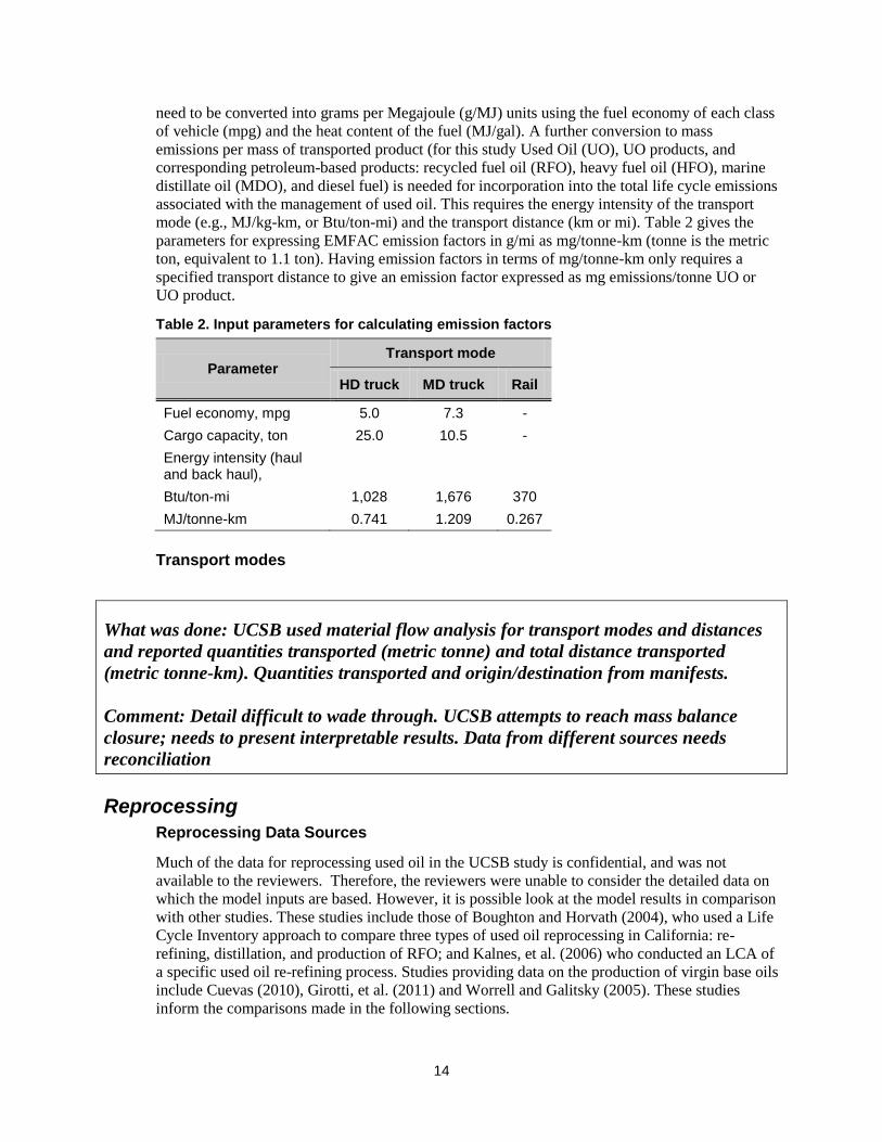
mode (e.g., MJ/kg-km, or Btu/ton-mi) and the transport distance (km or mi). Table 2 gives the
parameters for expressing EMFAC emission factors in g/mi as mg/tonne-km (tonne is the metric
ton, equivalent to 1.1 ton). Having emission factors in terms of mg/tonne-km only requires a
specified transport distance to give an emission factor expressed as mg emissions/tonne UO or
UO product.
Table 2. Input parameters for calculating emission factors
Parameter Transport mode
HD truck MD truck Rail
Fuel economy, mpg 5.0 7.3 -
Cargo capacity, ton 25.0 10.5 -
Energy intensity (haul and back haul),
Btu/ton-mi 1,028 1,676 370
MJ/tonne-km 0.741 1.209 0.267
Transport modes
What was done: UCSB used material flow analysis for transport modes and distances
and reported quantities transported (metric tonne) and total distance transported
(metric tonne-km). Quantities transported and origin/destination from manifests.
Comment: Detail difficult to wade through. UCSB attempts to reach mass balance
closure; needs to present interpretable results. Data from different sources needs
reconciliation
Reprocessing
Reprocessing Data Sources
Much of the data for reprocessing used oil in the UCSB study is confidential, and was not
available to the reviewers. Therefore, the reviewers were unable to consider the detailed data on
which the model inputs are based. However, it is possible look at the model results in comparison
with other studies. These studies include those of Boughton and Horvath (2004), who used a Life
Cycle Inventory approach to compare three types of used oil reprocessing in California: re-
refining, distillation, and production of RFO; and Kalnes, et al. (2006) who conducted an LCA of
a specific used oil re-refining process. Studies providing data on the production of virgin base oils
include Cuevas (2010), Girotti, et al. (2011) and Worrell and Galitsky (2005). These studies
inform the comparisons made in the following sections.

15
Products
The UCSB Final Report identifies several products resulting from the reprocessing of used oil.
Depending on the process used, the resulting products are:
Re-refined Base Oil
Marine Distillate Oil
Recycled Fuel Oil
Other fuels (light ends)
Asphalt flux
Ethylene glycol
These products are listed in Table 15 of the UCSB report, along with the quantities of each
produced in the 2010 Base Year and each of the three scenarios analyzed. The nature of the
materials and their yields for each scenario appear to be generally consistent with the published
literature.
Displaced Products
The reprocessing and use of collected used oil results in the displacement of other products.
Depending on how the used oil is reprocessed, one or more of the following products may be
displaced:
Virgin Base Oil
Diesel fuel (No. 2)
Heavy Fuel Oil (No. 6)
Natural gas
Bitumen and road oils
Ethylene glycol
All of these products, except ethylene glycol, are produced by refining petroleum. The quantities
of each displaced product for the base year and three scenarios are listed in Table 15 of the UCSB
Final Report. The quantities of displaced products generally appear reasonable, as they are
usually close to or identical to the secondary production figures for the reprocessing.
Displaced Emissions
The UCSB report is based on life cycle inventories for petroleum refining in the U.S. and
California. These inventories are described in the report Crude Oil Refining in U.S. and
California (PE International 2012, referred to hereafter as the PE report). This report references
an Excel workbook of inventory data that was also reviewed.
The PE report describes the process for allocating energy and emissions to various refinery
products, though the description is fairly general. A comment on the Draft Report noted that
specific results for the various refinery products from California and U.S. refineries were not
presented in the report. The Final Report addresses this comment by including a detailed

16
discussion of displacement and how displaced products were incorporated into the life cycle
assessment model in Appendix D.
REFINERY EMISSIONS
The refining data used in the model comes from various public databases containing air emissions
and water discharge data. These data are then normalized by dividing by the refinery throughput
of crude oil to obtain emission factors in terms of mass emitted per kilogram of crude processed.
For both the U.S. and California refineries, the quantity of crude processed is based on refining
capacity, that is, the maximum crude throughput under ideal conditions, rather than the actual
crude throughput. Since the air emission and water discharge data are based on actual 2010
operations, the calculated emission factors should be based on actual 2010 crude throughput.
Actual crude throughput is available for the U.S. from the Energy Information Administration.
Corresponding data is published for California in the annual compilations of its Weekly Fuels
Watch Reports. These data are summarized in Table 3. As this table shows, the actual crude
processed in both the U.S. and California was just 85 percent of the refinery capacity, meaning
the calculated emission factors based on crude throughput should be proportionately greater. This
difference between actual throughput and refinery capacity is not considered in the UCSB Final
Report.
Table 3. Crude oil distillation capacity and throughput for 2010
U.S. California
Atmospheric Crude Oil Distillation Capacity, Operable barrels/stream day
17,808,000 1,939,000
Actual Average barrels/day 15,177,000 1,644,200
Actual/Capacity 85% 85%
The PE report provides life cycle impact (LCI) data for a variety of energy products used in this
study through the GaBi model. In addition, PE provided a study of refinery modeling for
California and U.S. petroleum products. The study provides the basis for LCI data for displaced
products including:
Marine Distillate Oil
Light hydrocarbons (gasoline)
Heavy fuel oil
Diesel fuel
Lubricant base oil
GREENHOUSE GAS EMISSIONS
The calculated CO2 emissions factor for oil refining in California is approximately two-thirds
higher than the corresponding U.S. figure in the PE report: 0.362 kg/kg crude oil in California
versus 0.218 kg/kg crude oil for the U.S. average. While refineries do vary in their energy
consumption and emissions depending on the depth of refining, greenhouse gas accounting
practices can also have a large effect on the results, and it is not clear whether that is the case with
the data included in the report.

17
Oil refineries typically produce electricity as well as steam in their power plants. These plants
may operate as co-generation facilities providing steam to the refinery and selling excess
electricity to the grid. Alternatively, the refineries may have captive power plants for the
exclusive use of the refinery. In the former case, the emissions from the co-generation facility are
only partly attributable to the refinery operations. Such distinctions are often not considered for
regulatory reporting, however.
The production of hydrogen releases large quantities of greenhouse gases, but these emissions
may or may not be counted in the refinery totals. At the Chevron Richmond refinery, for
example, the hydrogen plant emissions are counted in the refinery totals. At Chevron’s El
Segundo refinery, in contrast, the Air Liquide El Segundo hydrogen plant reports independently,
even though it is a captive facility of the refinery. If the El Segundo refinery included the
hydrogen plant’s emission in its total, the refinery emissions would be almost 20 percent greater.
Even if it is not possible to address these kinds of discrepancies within the scope of the life cycle
assessment (LCA), they should be noted as a source of uncertainty, and assumptions as to
whether displaced products come from U.S. average or California refineries should be clearly
stated and documented where possible.
Refining emissions are just one part of the emissions associated with the displaced products.
There are also emissions associated with producing, treating, storing, and transporting crude oil to
the refinery. Instead of trying to obtain and compare data on each of the processes up to the point
of use, a more aggregated look at emissions from displaced use and displaced production for each
of the three scenarios is taken. The information in Table 4 is adapted from Table 32 of the UCSB
report and is discussed in the context of the three reprocessing options.
Table 4. Global Warming Potential for 2010 base year and three scenarios from UCSB study
In million kg CO2eq 2010
Base Year Extreme
Re-re Extreme MDO Extreme RFO
Collection & hazardous waste disposal
35.9 33.2 33.2 33.2
Reprocessing 56.9 105 49.7 1.39
Use of secondary products 513 76.0 581 972
Displaced use -508 -76.4 -581 -929
Displaced production -185 -309 -144 -204
Net results -87.5 -171 -61.0 -127
REFINERY LCI DATA
The displaced emissions from oil refineries are quite variable in LCA studies. The review team
examined the PE data for oil refining and compared well-to-tank greenhouse gas (GHG)
emissions as a proxy for emissions intensity since the primary sources of emissions from oil
refining are combustion sources. A review of UCSB’s use of the PE data indicated that crude oil
transport needed to be added to the model, which was accomplished in the final version of the
model as discussed in the Final Report. Examining the data in Table 5 indicates a range in
emissions from different studies, regions, and refined product types. The PE analysis shows lower
emissions for diesel and gasoline refining than indicated in other studies. This distribution of
emissions may be associated with the allocation method for emissions within refineries, although
the method is comparable to the approach taken in a study by Jacobs Consultancy (Keesom

18
2009). PE examined the emission intensity of Group 2 lubricants rather than Group 1 lubricants.
According to the study team, re-refining produces Group 2 quality lubricants. Interestingly, the
PE approach assigns relatively high emissions to heavy fuel oil (HFO). This emission intensity is
associated with HFO being the product of several refinery units.
Table 5. Well to tank GHG emissions from various LCA studies.
Model US
Diesel US
Gasoline US
HFO US
Lube CA
Diesel CA
Gasoline CA
HFO CA
Lube
PE 15.4 18.2 15.5 29.5 17.4 19.2 17.8 31.2
Jacobs 23.2 25.2 >25 >25
CA GREET (CARBOB) 20.85 21.48 14.82 25.56 19.82 22.74 13.78 25.12
GREET_1 18.89 18.96 12.14 17.16
Sources: PE International (2012); Keesom, et al. (2009); CA GREET (2009); GREET (2012)
Re-refining
The “Extreme Re-re” scenario corresponds to all of the reprocessed use oil being re-refined to
base oil. According to the UCSB study, of the total of 306 million kg of secondary production,
231 million kg, or 75 percent, was for re-refined base oil. This fraction is essentially equivalent to
the 72 volume percent cited in Boughton and Horvath (2004).
The UCSB Final Report states that 309 million kg of CO2e are avoided due to displaced
production. This is equivalent to 1.34 kg CO2e/kg base oil. This figure is in the range of that
given by Cuevas for life cycle emissions from the production of virgin base oil: 1.07 kg CO2e/kg
base oil. It is in the range of the figure given by Girotti et al. for the life cycle emissions from the
production of mineral base oil: 1.02 kg CO2e/kg base oil. (Though it should be noted the same
study gives a much higher figure for synthetic—polyalphaolefin (PAO)—base oil: 1.92 kg
CO2e/kg base oil.) Thus, we consider the UCSB calculations for global warming potential
(GWP) displacement from base oil production to be reasonable.
The emissions resulting from the use of fuels produced along with the re-refined oil is essentially
the same as the emission reductions from the fuel displaced (No. 2 oil). Thus, these emissions and
reductions have little effect on the net results. An independent check of the magnitude of the
GHG emissions from the displaced No. 2 oil agreed within 2 percent of the reported figure.
Distillation to Marine Distillate Oil (MDO)
The “Extreme MDO” scenario corresponds to all of the reprocessed use oil being distilled to
produce marine diesel oil, with a large amount of asphalt flux produced as a co-product.
According to the UCSB study, of the total of 288 million kg of secondary production, MDO
would account for 179 million kg, and asphalt flux would account for 109 million kg.
The UCSB Final Report indicates that use of the produced MDO would result in a GWP of 581
million kg of CO2eq from the combustion of secondary fuels. This is identical to the avoided
GWP from the avoided combustion of displaced primary fuel, No. 2 diesel fuel. Our own
calculation of the emissions and reductions was slightly larger — 606 million kg of CO2eq — but
still within 5 percent. And because the emissions and displacement cancel each other out, the
difference has no net effect.

19
Additional emission reductions result from displaced production. This figure accounts for the
emissions that occur upstream of the use of the displaced No. 2 oil. (For motor fuels, this would
be referred to as the “well-to-tank” emissions). A preliminary review of the UCSB data on
refinery emissions related to the production of the displaced oil appeared to indicate that the
UCSB emissions were much smaller than indicated by other studies. Emissions from the well to
the refinery, however, appeared to be somewhat larger. For this study, the more important figure
is the accuracy of the total upstream emissions to the point of use, rather than the individual
processes that make up that total.
Dividing the displaced production global warming potential (GWP) emissions (62 percent of 144
million kg CO2e) by the displaced use emissions (581 million kg CO2e) shows that the production
emissions in the UCSB model amount to 15 percent of the emissions from combusting No 2 oil.
This figure is somewhat less than the corresponding figure for the GREET model (California
GREET1.8b), which indicates that, for conventional diesel fuel, the upstream emissions to the
point of use are equivalent to 27 percent of the emissions from burning the fuel. The GREET
figures suggest that in the Extreme Marine Distillate Oil (MDO) scenario, the displaced
production emissions for No. 2 oil could be more than 90 percent greater than are reported (170
vs. 89 million kg CO2e), with a corresponding emission reduction in the net results.
Recycled Fuel Oil (RFO)
The “Extreme RFO” scenario corresponds to all of the reprocessed oil undergoing minimal
treatment to be sold as recycled fuel oil. According to the UCSB figures, the 325 million kg of
secondary production in this scenario would result in the displacement of 104 million kg of No. 2
oil, 111 million kg of No. 6 oil, and 92 million kg of natural gas. The mix of these fuels is driven
in part by market forces that are outside the scope of this review.
Our analysis of the energy content of the displaced fuels and the secondary production of RFO
indicated that the energy content of produced fuel and the sum of the displaced fuels matched
within 1 percent, thereby indicating the overall reasonableness of the displacement quantities for
this scenario.
The combustion of the recycled oil is reported to result in global warming potential (GWP)
emissions of 972 million kg CO2e. This figure appears to be slightly low. Our own calculation,
assuming emission characteristics averaged between No. 2 and No. 6 oil results in emissions of
1,033 million kg CO2e, slightly more than 6 percent greater than the UCSB figure. (Had the
emission factor for No. 2 oil been used, our results would still be 6 percent greater than UCSB’s).
The displaced oil emissions reported by UCSB for the No. 6 and No. 2 oils and natural gas
amount to 929 million kg CO2e. Our own calculation agreed with this figure to within a fraction
of 1 percent.
The accuracy of the displaced emissions from production of the displaced fuels is more difficult
to assess as the reductions in emissions are not reported for each fuel separately. Overall, the
upstream production emissions are equal to 19.6 percent of the combustion emissions for the
respective fuels. As noted above for No. 2 oil, the GREET model indicates a corresponding figure
of 27 percent, and upstream natural gas emissions are often reported to be a similar magnitude.
While production emissions of No. 6 oil would be less than this figure, they would have to be far
smaller to bring the average value down to that used by UCSB for this scenario. Thus, although
we cannot provide a calculation of the extent to which the displaced production emissions in the
UCSB analysis differ from those calculated from GREET, it appears that the difference is still
significant but in percentage terms not quite as great as for the Extreme MDO scenario. It bears
noting that the well-to-tank emission factors for the production of various refinery products used

20
in the UCSB analysis (taken from the PE refinery model) differ from those defined in GREET
(see Table 134 of the UCSB Final Report).
Rejuvenation
Rejuvenation only applies to used dielectric oils. The advance draft report states: “displaced
production and use is not modeled for dielectric oil rejuvenation, which is regarded as life time
extension.” This leaves two options: dielectric oil is either not yet a used oil, or it is used oil. If it
is, then the fraction of the market that is rejuvenating dielectric oil is a variable in the model with
market volume and production impacts that need to be evaluated. This market impacts may still
be negligible and, therefore, disregarded, but only if the evaluation proves this to be the case.
More context is needed.
Dispose as Hazardous Waste
The data discussed in the UCSB report regarding this topic were for 2010. A brief note on why
2010 data were deemed to be representative of all years would be helpful. There is no reason to
suspect that 2010 is not a representative year, but a short note to substantiate this assumption
would suffice.
The biological degradation of the carbon in used oil disposed in an anaerobic municipal solid
waste (MSW) landfill to methane and carbon dioxide is likely to be quite slow. Oil that reaches
an MSW landfill in any year is likely to produce little or no methane in the year of its burial.
Hence, there are two questions for the UCSB study:
What is the methane generation potential for the carbon in used oil?
How should that methane generation be modeled under the static annual environmental
impacts modeling portrayed in the GaBi Envision models?
Morton Barlaz at North Carolina State University has done much work on modeling degradation
versus long term storage of the biogenic carbon in biogenic carbon containing materials buried in
an anaerobic MSW landfill. He may have some insights on the likely fate of the fossil carbon in
used oil buried in an MSW landfill. He may also have some insights on the fate of used oil
disposed in the typical hazardous waste landfill. This may be helpful in deciding how to estimate
methane release from illegal disposal in an MSW landfill or legal disposal in a hazardous waste
landfill. The methane benefits of decreasing disposal of used oil, whether legal or illegal, need to
accurately reflect the short term methane generation rate for methane from used oil, rather than a
long term release rate that will only occur over 100 years or more. At a minimum, the model
should reflect the difference between short- and long-term methane reduction potentials from
policies to decrease landfill disposal of used oil.
Improper Disposal
Section 4.10.3 of the UCSB report on used oil combustion with municipal solid waste (MSW) in
MSW incinerators assumes there are no hydrocarbon emissions from burning used oil. This
seems highly unlikely given start up and shut downs, upsets and the days when MSW arrives with
very high moisture content. In all these situation complete carbon and hydrocarbon combustion
seems likely to be inhibited. There are several data sources for MSW incineration emissions
available—e.g., AP-42 (EPA 1995), the EPA/RTI MSW Decision Support Tool (DST) database;
and emissions data reported by the three California incinerators (or surrogates such as Metro
Vancouver MSW incinerator in Burnaby, British Columbia, the Marion County MSW incinerator
in Oregon, and the several MSW incinerators in Massachusetts). Although these emissions may
be small and not rise to the level of a regulatory limit, they should still be addressed in an LCA.

21
In many cases, life cycle assessments are comparing activities or management options that all
meet regulatory standards and it is the low level pollutant emissions that can accumulate to favor
one option over another in terms of environmental impact.
Assumptions used in the improper disposal model seem appropriate in general. The Appendix C
illegal dumping model also seems well reasoned given the lack of information.
In Section 11.2.5 of the UCSB report there is some concern that the model, by the way it
distinguishes coastal from inland counties, may underestimate impacts to freshwater, assuming
the final disposition is the ocean. The 81 percent disposal in seawater seems far too high. Santa
Cruz County, for example, has a large coastline. But it also has several long freshwater courses
that improperly disposed oil pass through en route to the ocean. This is mentioned and could be
modified with a few basic assumptions about how some oil might be retained in freshwater
system. By default assuming 81 percent goes to the ocean seems to be an over-estimate.
However, there does not seem to be an objective rationale for changing this approach. Given that
most toxicological studies look at freshwater impacts, the impacts on oil disposed in ocean water
may be over-estimated according to the UCSB team. This seems like an appropriate tradeoff.
Pathways for Improper Disposed Oil
The model for improperly disposed used oil is divided into three principal pathways: waterway
(W), landfill (L), and soil (S). According to the UCSB report, no information was available to
suggest how much oil is disposed of by each pathway, and thus each of the three is modeled with
equal weight (33 percent). A brief review of the literature shows that there are reports that may
give some indication of the amount oil entering these pathways, and thus provide a more
meaningful split among the pathways than a simple assumption that the oil enters each equally.
For example, the total amount of used motor oil improperly disposed (not including vehicle leaks)
was described in a presentation to the March 2004 Used Oil Recycling/Household Hazardous
Waste Conference (Browning 2004).
For the landfill (L) pathway, the California 2008 Statewide Waste Characterization Study report
(CIWMB 2009) includes data on the tons of used motor oil disposed of as solid waste and the
tons of steel in oil filters disposed of as solid waste. Depending on whether the data are for used
oil and filters collected through municipal hazardous waste collection programs or represent
sample data of municipal solid waste headed to disposal, the data in the report may be used to
give a rough idea the quantity of improperly disposed of oil as oil or as residual oil in oil filters.
For the waterway (W) pathway, the California Environmental Protection Agency (Cal/EPA)
report on the Characterization of Used Oil in Stormwater Runoff in California (Cal/EPA 2006)
provides estimates of the total annual loading of oil and grease to state waters as well as
information on the contribution of used oil to the total load borne by runoff. This report also gives
an indication of the amount of used motor oil entering waterways from vehicle leaks as opposed
to intentional, improper disposal.
The distinction between oil that is leaked into storm drains from vehicles and oil that is
intentionally disposed of in these drains is important for two reasons. First, any policy changes
related to the handling of oil drained from vehicles will not affect the quantities leaked into the
environment from these vehicles. Second, leaks represent a widespread, but low level
introduction of the oil into the environment, while intentional dumping to storm drains (or soil)
represent a large localized release. The environmental effects of these two different types of
releases will also differ. Thus, it is recommended that the two flows to storm drains be accounted
for separately.

22
Improper disposal to soil (S) appears to have received the least amount of study, based on the
available literature. Some projections of how much product enters this pathway may be able to be
inferred from the difference between the total amount of oil improperly disposed and the
estimated amounts entering the other pathways using other studies such as those noted above.
WATERWAY PATHWAY
The model contains a number of assumptions related to the waterway pathway that deserve
further explanation:
Of the oil entering storm drains, 20 percent is assumed to be diverted to wastewater treatment
plants. This figure is based on the population of coastal counties with diverted drains, but
appears to be applied to the whole state. Also, drain diversion remains a work in progress,
and it is not clear that all of the oil in runoff from these communities is diverted. In short, the
assumption of 20 percent diversion of oil entering storm drains needs greater explanation and
justification. In particular, the estimate seems to be over-representing this flow because it is
based on installed capacity, not actual throughput. If these systems only work during dry
weather, some accounting of the frequency of operation (frequency of conditions that allow
re-directing to wastewater treatment plants) must be incorporated into the probability
assessment as well.
Of the oil entering storm drains, 7 percent is assumed to enter filtered drains. The source for
this figure should be cited and the methodology to apply the figure statewide should be
explained. In addition, there is no accounting for the filtration system for functionality. There
should be an assumption or at least sensitivity for fouled filters, filters not working properly,
and the like. This feedback was not addressed in the Final Report, but may be inconsequential
given the other assumptions made in the improper disposal model.
Removal efficiency for the filtered storm drains comes from manufacturer data for one
particular type of drain. Some discussion of the relevance of these data to the drains used in
California should be given, particularly since the effectiveness of such drains depends highly
on how well they are maintained and their age (if efficiency declines with time).
Treatment efficiencies for wastewater treatment are reported to come from the U.S. EPA Risk
Reduction Engineering Laboratory (RREL) Treatability Database (for oil diverted to
wastewater treatment plants,
http://iaspub.epa.gov/tdb/pages/contaminant/findContaminant.do), which is a database for
drinking water treatment. It is not clear that the treatment efficiencies reported in this
database are relevant to California wastewater treatment plants.
The ratio of used oil disposed to freshwater versus seawater seems too small, as mentioned above.
The methodology used to justify the ratio assumes that San Francisco Bay Area counties are
coastal counties when much of the region drains freshwater. The impacts to freshwater are
therefore underestimated. There is mention of used oil passing briefly through freshwater in these
coastal counties, but the time used oil spends in freshwater in coastal counties is probably much
higher than the zero currently allotted to it. This could have significant impacts because the
quantities of used oil would have more ecological impacts in freshwater bodies than in the ocean.
LANDFILL PATHWAY
The landfill (L) pathway represents used oil disposed of in municipal solid waste (MSW). The
model seems to assume that all of the municipal waste is landfilled, with some residuals being
incinerated. (The pathway to incineration is through landfilling). California has several waste-to-
energy plants, however. Even though the actual and potential amount of waste oil that could be

23
directly combusted in these facilities is small, it would be more accurate to include the direct
combustion of the oil in the model:
The Columbia University Municipal Solid Waste Database:
(http://www.seas.columbia.edu/earth/recycle/) indicates 1.2 percent of California’s MSW is
combusted in waste to energy plants.
The total capacity of the three MSW waste to energy plants in California amounts to
approximately 3 percent of the amount of waste landfilled in 2011.
In addition, Section 4.10.3 of the UCSB report states that the landfill gas emission capture
efficiency from the landfill is 30 percent in 2010, with the value increasing over the next 20
years. However, the GaBi model uses 25 percent for 2010, 75 percent for 2015 and 90 percent in
2020. In addition to the disagreement between 2010 values, one reviewer questions the wisdom of
using the projected values in the GaBi model. The increase from 25 percent (or 30 percent) to 75
percent seems unlikely and should be justified.
Moreover, given the 20-year time horizon, the question arises concerning which IPCC global
warming potential (GWP) is used to incorporate methane into the greenhouse gas impact
calculation, the 20-year GWP or the 100-year GWP?
IMPROPER DISPOSAL SUMMARY
In summary, the improper disposal of used oil is an important pathway that in the model that
deserves further explanation. Rather than simply assuming key values in the modeling of this
pathway, the literature—particularly studies relevant to California—should be reviewed more
thoroughly to make use of the information in them. In this way, the starting point for the
sensitivity analysis will be past research rather than raw assumptions.
In addition, the terminology used for describing the informal management extreme management
sensitivity analyses is somehow misleading. These are not four extreme scenarios; rather, it is a
single extreme scenario with four different sensitivity analyses on its main parameters.
Oil Demand and Collection Categories
The quantities of used collected in California are important inputs into the model because the
quantities of oil improperly disposed of are calculated as the difference between oil demand, and
used oil collected and otherwise accounted for. The UCSB Final Report identifies three categories
of oil demand: passenger car motor oil, heavy duty motor oil, and industrial oil. The report states
that the first two categories correspond to “lubricating oils” as defined for California’s Used Oil
Recycling Program (CCR Section 18601), while the third category corresponds to the regulatory
definition of “industrial oil” plus dielectric oils.
Section 4.7 of the advanced Draft Report states that the demand for industrial oil in 2010
amounted to 82.7 million gallons. If the intent of this figure is to correspond to the regulatory
definition of industrial oil plus dielectric fluid, then it appears to overstate the actual quantity. The
reason for this overstatement is that the figure of 82.7 million gallons is based on the definition of
industrial oil used in what has become known as the Kline Report (Kline 2012 Confidential and
Proprietary), which differs from the CalRecycle definition. The Kline definition of industrial oil,
for example, includes consumption in stationary and mobile industrial internal combustion
engines. By California regulation, these are considered “lubricating” oils rather than industrial
oils (CCR 1860.1).

24
The Kline report recognizes the differing definitions of industrial oil, and provides an adjusted
figure to correspond with CalRecycle’s definition. That figure is 63.4 million gallons for 2010, or
almost 20 million gallons less than used in the UCSB report. However, the Final Report provides
sufficient explanation justifying the quantity employed.
Improper Disposal Model
The UCSB report presumably (needs to be clarified) assumes that 15 percent (0.3kg/2kg) of the
improperly disposed used oil goes directly to a municipal solid waste (MSW) landfill. Of the
remaining, the report assumes half (50 percent) goes into the soil and half is spilled onto road
surfaces (asphalt), which ultimately becomes found in storm water runoff. As noted above, 81
percent of this runoff represents discharges to seawater, the remainder to fresh water, wastewater
treatment, or landfill.
The UCSB report does not mention direct flows into water bodies as a potential fate. The report
seems to assume that dumping passes through storm drains and sewers, which only exist in
incorporated areas of California. It would be more appropriate to assume a portion directly enters
waterways without passing through storm drains and sewers. This is important due to the
filtration assumption in the current improper disposal model. There should be a water route that
directly leads to deposits in fresh or ocean water.
Other comments on the direct discharge to water pathway are:
Clarify why it matters if disposed oil is deposited on agricultural soil or industrial soil (are
these limitations imposed by the impact category?). In section 11.2.8 of the Final Report it is
noted that this is an unimportant distinction, so does not warrant more clarification. .
Is there a better way to develop a weighting between the proportion splits between soil and
water? This will be an important sensitivity to analyze and should involve scenarios where all
(or maybe 90 percent) or emissions go down each pathway. Based on the comments in
section 11.2.8 it appears that this is not an important sensitivity.
The fate of the unfiltered improperly disposed oil sent down the storm drain was unclear in
the Draft Report. Because fates are determined by the TRACI model, this did not warrant
being addressed in the Final Report.
Valence state of metals
The TRACI 2.0 model that is employed for environmental impact characterization requires that
metal valence be identified in its characterization factors for metals, particularly chromium and
vanadium. There was some discussion of the hexavalent chromium (Cr+6
) being overestimated
because Cr+3
is more commonly a product of combustion. Further research on the long-term fate
of chromium should be done here. Some brief research by a review team member shows that with
minimal effort (UV irradiation, increased temperature) Cr+3
can become Cr+6
, while the
remediation research suggests going in the other direction (reduction of Cr+6
to Cr+3
) is quite
challenging. This emphasizes the need for metals valence data for discharges and their ultimate
fate should be investigated.
Feed and Product Transport
The UCSB report notes that GREET emissions factors were changed to reflect conditions.
Discussion regarding how these emissions factors differ from the California-modified GREET
emissions factors used in California’s low carbon fuel standard should be provided.

25
In addition, in instances in which transport emissions factors will vary over time, will these be
based on emissions from new vehicles produced? Or an average from the fleet at any given time?
This characterization could use better clarification in the Final Report. In the Final Report it is
noted that the emissions factor takes into account fleet turnover.

26
Emission Factors and Life Cycle Data This section describes the reviewer’s comments on emission factors and life cycle data. The
emissions factors that received the greatest attention were for combustion emissions. In part to
address these UCSB developed a combustion emissions model that focused on a comparison of
the emissions of recycled fuel oil (RFO) to heavy fuel oil (HFO) derived from petroleum refining.
Combustion emissions factors derived from this model, combined with data to support
combustion model development, and data from other sources were documented in the advance
draft report. Thus, the critical review effort focused on these two elements: the combustion model
and the set of emission factors documented. These reviews are summarized in the following
subsections.
Combustion Emissions Model
As noted in UCSB’s documentation, the combustion of used oil is a significant contributor to the
overall environmental impacts of the used oil management system studied, although existing life
cycle inventory databases were found to be inadequate with respect to accurately representing
these processes. The UCSB study team therefore developed a detailed, parametric combustion
model for RFO and HFO for the life cycle assessment (LCA) based on a review and analysis of
various data sources, primarily existing literature and public databases, as well as some
proprietary databases and with stakeholder consultation. The majority of the data were from 2006
or more recent. The model considers both the composition of the used oil burned and the
combustion technology based primarily on U.S. fuels and practices. Where applicable, air
pollution control technologies are also considered. Combustion of used oil, RFO, and distillate
co-products are modeled in comparison with the combustion of primary fuels assumed to be
displaced by these co-products. These included No. 2 distillate, No. 6 residual oil, and natural
gas. Except for differences due to fuel composition, MDO produced from used oil was assumed
to combust identically to primary MDO. The results of the combustion model are emission
factors and retention rates, by combustion technology and fuel type, for criteria and toxic air
emissions resulting from the combustion of recycled (re-refined) fuel oil and heavy fuel oil.
The combustion model was developed around a set of fuel-specific emission factors for eight key
combustion pollutants, and technology-specific retention rates for selected elements and
compounds whose emission factors are dependent on fuel composition. No new primary data
collection was performed for development of the combustion model. The modeling of fuel
combustion is therefore limited by data availability and relevance.
Based on the significance of combustion emissions to the model results and the uncertainty in the
data, sensitivity analyses were conducted for both emission factors and retention rates using upper
and lower bounds for emission factors and retention rates based on analysis of primary data.
Additionally, due to the uncertainty of the limited data for used oil combustion, ranges of
emissions factors and retention rates, by fuel type and combustion technology, were also
estimated and used in sensitivity analyses.
A detailed review of the report’s RFO and HFO combustion model is provided below. The
review considered the overall modeling methodology and data analysis used, as well as data
sources with respect to completeness, representativeness, and applicability. While the overall
output of the combustion model has not changed from the draft version (i.e., emission factors and
retention rates by combustion technology and fuel type for criteria and toxic air emissions from
the combustion of RFO and HFO), the development of the model has been revised with respect to

27
documentation of data sources, model implementation and data analysis. The draft combustion
model and documentation were distributed for review to the critical review team and interested
stakeholders and where appropriate, input and comments received from the stakeholder review of
the draft were incorporated into the final version of the recycled fuel oil (RFO)/heavy fuel oil
(HFO) combustion model. The revised combustion model documentation is a marked
improvement over the draft version and provides a more focused and detailed description of the
modeling methodology, data sources and analyses, and results including comprehensive graphical
summaries of combustion emissions data by fuel type, fuel composition, and combustion
technology. Estimated emission factors and metal retention rates from the model, including
expected upper and lower bound estimates, are well summarized in tabulated and graphical
formats. Additionally, limitations associated with the methodology, data sources, and results of
the combustion model are summarized in the Final Report.
Modeling Methodology
IMPLEMENTATION
The methodology implemented in the final version of the combustion model was not significantly
altered from the draft version and was developed to meet the following objectives:
Empirical basis—develop credible and scientifically-sound estimates of emission from used
oil combustion based on data and measurement from primary data sources;
Incorporation of fuel composition—develop fuel-specific estimates due to expected
differences in emissions associated with differences in used oil composition;
Parametric model implementation—large uncertainty in the limited data and wide disparity
among data sources require evaluation with sensitivity analysis facilitated by a parameterized
model structure
Consistent use of lower heating value (LHV) equivalency—emission factors based on
consistent use of the LHV for fuels, considered indicate of the functional utility of the fuel for
modeling displacement (This reviewer notes an inconsistent reference to the higher heating
value in the combustion model documentation (Section 10.2.4), which is assumed to be a
typographical error)
The modeling approach separated combustion emissions into three categories: emission
calculations based on retention rates, calculations based on average emissions factors by fuel type
only, and emission calculations based only on technology. These categories are intended to
describe the modeling approach taken for a given emission, not the flow’s inherent properties.
The division is made for modeling simplification purposes.
In the UCSB model, combustion emissions are calculated per mass of fuel burned with emission
factors expressed as mass of pollutant emitted per mass of fuel burned. While certain emissions,
such as heavy metals, can be estimated based on fuel composition and retention rates for different
combustion technologies, given the lack of extensive data many of the emission estimates are an
average of all the representative emission data available for a given fuel. In a few cases, the type
of combustion source and any associated control technologies are the critical factors in
determining emission rates and were therefore estimated based on combustion technology alone.
The emissions estimation methodology used for the combustion model based on composition,
and/or technology-dependence, represents a trade-off between technical accuracy and data
collection efforts and is a reasonable modeling approach for the study.

28
COMBUSTION TECHNOLOGIES
As discussed in AP-42 (EPA 1995), the primary types of fuel oil burned by combustion sources
include distillate oils and residual oils. These are further distinguished by grade numbers, with
Nos. 1 and 2 being distillate oils while Nos. 5 and 6 are residual oils. Fuel oil No. 4 is typically
either distillate oil or a mixture of distillate and residual oils. Distillate oils are more volatile and
less viscous than residual oils. They have negligible nitrogen and ash contents and usually have
low sulfur content (by weight). Distillate oils are used mainly in domestic and small commercial
applications, while residual oils are used mainly in utility, industrial, and large commercial
applications. The recycled fuel oil (RFO) combustion model developed for the project considered
primarily those combustion technologies associated with the heavier residual fuel oils for the
development of emission factors and retention rates.
UCSB reviewed emissions and emission factor data from a number of sources (discussed below)
for combustion devices/technologies which support the use of liquid petroleum fuel oils. These
include industrial boilers, commercial/institutional boilers, space heaters, asphalt plant kilns,
cement and lime kilns, and steel production blast furnaces. Where applicable, combustion devices
which incorporate the use of various air pollution control (APC) technologies are also included in
the analysis. The heavy fuel oil (HFO)/RFO combustion model estimates technology-specific
average emission factors and retention rates for criteria pollutants, particulate matter, and trace
metals based on an analysis of all relevant data for each combustion technology. It was noted that
most of the data available for model development were for fuel oils combusted in boilers and this
represents a general limitation in the technology-specific emission factors and retention rates.
Emission factors are estimated for RFO and its displaced product, HFO (fuel oil No.6), and
compared with emission factors for other distillate fuel oils extracted from existing data sources
(primarily AP 42 as discussed below).
When considering comments about the relative combustion emissions factors, the UCSB staff
should keep in mind that emissions from combustion and the ultimate fate of emissions may yield
different values. Concern for example from NORA suggested the sulfur emissions may be too
high. Where appropriate, it may be helpful to incorporate more justifications where there are
comments from stakeholders.
AIR POLLUTION CONTROL TECHNOLOGIES
The oil combustion model developed for the study considers a number of particulate matter (PM)
control technologies based on the available data. These include fabric filters or bag houses;
cyclones, in which dust-laden gas is spun in a cylindrical collector that causes large particles to
transit to the edges for removal; venturi scrubbers, in which the gas stream is passed through a
liquid that absorbs pollutants; and electrostatic precipitators (ESPs), which use static electricity to
remove particulates as they pass through an electrical field.
UCSB’s analysis of the data showed that, in general, batch asphalt plant kilns utilize bag houses
(fabric filter) while cement kiln typically use ESPs for PM emission control. Particulate matter
control technologies for large boilers generally include ESPs, venturi scrubbers or cyclones.
Although the inclusion of PM emission control technologies in the combustion model is likely
more relevant and lead to larger impacts on the estimated results, control technologies for other
pollutants (i.e., NOx, SO2) should also be considered, or evaluated for use in the combustion
model.
In the development and implementation of the combustion model, emissions are calculated as a
mix of the combustion and emission control technologies discussed above. The current model
implementation requires assumptions regarding the use of RFO combustor PM controls in

29
California. Table 6 shows the fraction of recycled fuel oil (RFO) combustors in the state by
combustor category and presence of PM controls. UCSB indicated the distribution given in Table
6 is based on expert knowledge. While the RFO combustion technology split data shown in Table
6 were provided in the draft combustion model documentation, no reference was made to what
data were used in the final version of the model. The authors note the model was developed with
variable parameters to allow sensitivity analyses including this combustion technology split for
RFO. The default values used in the life cycle assessment modeling scenarios should be noted in
the Final Report. The study authors appropriately note the large uncertainty regarding these
assumptions requires further review and evaluation with sensitivity analyses.
Table 6. Assumptions applied in LCA for end use of RFO in California.
Combustion Technology % of RFO Combustors
Atomizing space heater with no control 2.5%
Vaporizing space heater with no control 2.5%
Boiler with control 10%
Boiler with no control 25%
Asphalt Plant with bag house filter 50%
Cement Kiln 10%
DATA SOURCES
The RFO/heavy fuel oil (HFO) combustion model is based on a variety of data sources, primarily
existing literature and public databases, as well as some proprietary databases and with
stakeholder consultation. Data were collected and reviewed for pollutant emissions and emission
factors by fuel type (distillate and residual fuel oil, waste oil, used oil) and combustion
technology. Additionally, data for retention rates of trace heavy metals by fuel type/composition,
and combustion device were collected and included in the analysis. The data sources used in the
model development include:
MACT—Boiler MACT Draft Emissions and Survey Results Databases.
http://www.epa.gov/ttn/atw/boiler/boilerpg.html.
Entropy—Entropy, Inc. for National Oil Recyclers Association. Quantification of Metals
Emissions from Burning Used Oil Fuel. Research Triangle Park, NC. 1996.
Dyke/Lubrizol—Dyke, P. Emissions from Small Waste Oil Burner Burning Drained
Lubricating Oil. 2012.
Shaaban & Salvani—Shaaban, A. H., & Salavani, R. (1996, August). Heat recovery of used
petroleum, oil, and lubricants (POL). In Energy Conversion Engineering Conference, 1996.
IECEC 96, Proceedings of the 31st Intersociety (Vol. 3, pp. 1950-1955). IEEE
AP-42 (EPA 1995)—Compilation of Air Pollutant Emission Factors, Volume 1: Stationary
Point and Area Sources, AP-42, Fifth Edition, U.S. Environmental Protection Agency, Office
of Air Quality Planning and Standards, Research Triangle Park, North Carolina, January,
1995.

30
Vermont Agency of Natural Resources—Vermont Agency of Natural Resources, Vermont
Department of Environmental Conservation. Vermont Used Oil Analysis and Waste Oil
Furnace Emissions Study. Waterbury, Vermont. 1996
GHG Protocol—“Emission Factors from Cross-Sector Tools”, version 1.3 (2012)
The data set used for the draft version of the model included 6,724 distinct measurements of fuel
composition or heating value and 3,602 emission measurements, representing a total of 1,003
tests at 302 facilities. Overall, 67 percent of the tests were conducted 2006 or later. Seventy-eight
percent of the composition measurements and 71 percent of the emission measurements were
from the tests conducted in 2006 or later. These data were updated for use in the final version of
the model as documented.
An updated Excel workbook, exported from the Matlab® data analysis software used for the
model development, was provided with the model documentation for review. A master table of all
composition measurements from all sources, reported in uniform units of kg pollutant per kg of
fuel, was included, and accompanied by various supporting data sheets and summaries. All
relevant data extracted from the sources referenced were included and tabulated by facility, date,
data source, combustion device, and fuel type, as appropriate. A summary of the data available
and used in the analysis, by fuel type and control technology and sample populations was
provided in the model documentation.
As noted above, the combustion model groups emission and emission factors into a limited
number of bins by combustion technology, including any applicable air pollution control (APC),
as well as fuel type. The data collected and reviewed for the development of the combustion
model are summarized below. Data sample counts and data sources are further documented in the
UCSB Final Report. Similar summary data tables by air pollution control technology (NOx or PM
control) were also available with the model documentation for review.
A brief review of the various data sources referenced in the development of the recycled fuel oil
(RFO)/heavy fuel oil (HFO) combustion model was conducted and is summarized below. A
complete summary of the data sources used for the development of the RFO/HFO combustion
model, including combustion technology and applicable control equipment, is provided in Table
128 of the UCSB Final Report.
MACT
Area source industrial, commercial, and institutional boilers are subject to rules based on
emission limits and maximum achievable control technology standards (MACT) as required
under Section 112(d) of the Clean Air Act (CAA) and the national emission standards for
hazardous air pollutants (NESHAPs) for major and area combustion sources. Relevant data for
the study were obtained through the EPA’s Air Toxics Website (ATW) as two linked databases
including data regarding composition of the various fuels used in industrial, commercial, and
institutional boilers; stack testing data; and information regarding the boiler devices and any
control technologies installed. Each MACT composition and emission data point represents a
single facility, parameter, and date of measurement and, for combustion emissions, a specific
combustion device. All fuel composition and combustion emissions are converted to consistent
set of units (i.e., kg emission per kg fuel combusted) using the lower heating value (LHV) for the
fuel as appropriate. The MACT databases provided recent measurement-based fuel composition
and emissions data for the development of the combustion model.

31
Entropy
Entropy completed a report titled “Quantification of Metals Emissions from Burning Used Oil
Fuel” for the National Oil Recyclers Association in 1996. This study evaluated the release of
metals from used oil combustion. The metal content of the used oil combusted was also
considered and results reported in terms of the metal removal efficiency of the combustion
technology. Data from this source are directly applicable to the recycled fuel oil(RFO)/heavy fuel
oil (HFO) combustion model although it is nearly 20 years old.
Dyke/Lubrizol
This study tested the combustion of used oil in a small vaporizing space heater. Fuel samples are
analyzed and emissions of criteria pollutants, metals, dioxin/furans, and organic compounds are
reported. Results include fuel composition, and emissions, and metal retention rates for the
combustion of two different test samples from 2007.
Shaaban & Salvani
This study conducted for the U.S. Air Force/Department of Defense was published in 1996 and
documents composition and emissions from combustion of various type of used oil mixed with
diesel in an atomizing boiler.
AP-42, 5th Edition (EPA 1995)
The EPA maintains numerous documents and resources for the development and estimation of
emission and emission factors, including various combustion processes in Compilation of Air
Pollutant Emission Factors, Volume 1: Stationary Point and Area Sources, AP-42, Fifth Edition
(EPA 1995). Specifically, Chapter 1.3, Fuel oil combustion, and Chapter 1.11, Waste oil
combustion, provide fuel composition information and emission factors for used lubricating oils,
distillate oils, and residual oils. Although the fifth edition dates to 1995, EPA periodically
supplements and updates the publications. The latest versions of the relevant AP-42
documentation are from 1996 for waste oil combustion and 2010 for fuel oil combustion. These
data were considered by UCSB in the development of the combustion model and used when
appropriate, specifically for waste oils and heavy residual fuel (for HFO combustion). It is noted
that AP-42 air pollutant emission factors, specifically for fuel oil and waste oil combustion, are
routinely adopted in various studies and regulations.1,2
Vermont Agency of Natural Resources
Although conducted in 1996, this study provided information and data regarding the combustion
of used oil in space heaters including emissions of metals and fuel composition.
GHG Protocol
The Greenhouse Gas Protocol provides estimates of methane and nitrous oxide emissions by fuel
type, including used oil, No. 2 distillate oil and Nos. 4 and 6 residual fuel oils. Greenhouse gas
emissions were considered independent of combustion technology although both methane (CH4)
and nitrous oxide (N2O) are known to decrease with increasingly complete combustion.
1 http://www.iiasa.ac.at/~rains/PM/docs/documentation.html
2 http://www.ec.gc.ca/inrp-npri/default.asp?lang=En&n=B66DA62F-1

32
DATA PROCESSING AND ANALYSIS
UCSB provided a brief description of each of the data sheets included in the Excel workbook as
well as a discussion of the various calculations and data analysis steps used in estimating
emission factors and retention rates. Documentation was provided for how the data were grouped,
application of any corrections, and handling of non-detects and detection limits. Additional data
processing details relevant to understanding the modeling results were further documented for the
final version of the model version. The data, processing steps, and model implementation
descriptions were reviewed and found to support the combustion model development as
documented.
The UCSB combustion model supports four approaches for dealing with non-detects: omit from
data entirely, interpret as zero, assume a quantity equal to half the detection limit, and assume a
quantity equal to the detection limit. The model currently assumes half the detection limit for all
non-detects in which the detection limit is known to the model, both for composition and
emission measurements, independent of the data source. Only non-detects in the MACT, Entropy,
and Vermont data sources are treated in the current model version.
While the model includes non-detects (when a measurement was performed with no result) in the
data, non-measurements (when no measurement was performed) are excluded. The model
developers indicated only modest effects on the results due to the approach used and noted
possible sensitivity analyses may be include in later versions. A summary of the results for
alternative non-detect approaches was provided for evaluation.
In Appendix F, one reviewer suggests that a sensitivity analysis should be employed to the use of
the USLCI data, since they are old, and tend to not be very complete. This reviewer suggests
using U.S.-Ecoinvent data (Ecoinvent with U.S. background data, or GaBi data for these U.S.
energy inputs), to assess the impact of the use of different data sources. That discussion can be
added to the section on sensitivities.
This reviewer also suggests that data sources be cited for the primary recycling data. This
reviewer also recommends citing suggestions for future research to prevent having to use data
with quality 4 and 5 in future research? Data of quality 4 and 5 seem to be inappropriate for use in
any life cycle assessment (LCA).
COMBUSTION MODEL SUMMARY
Based on a review of the combustion model and documentation, the methodology used by UCSB
in the development of the model—to capture any significant variation among fuel type,
combustion devices and control technologies relevant to the study while minimizing total number
of groupings—provides a reasonably robust modeling approach to estimating emission factors for
recycled fuel oil (RFO)/heavy fuel oil (HFO) combustion given the available data. In general, the
objectives of the combustion model for use in the used oil LCA study as documented are satisfied
given the limited available data and provide reasonable estimates for the study, as well as a tool
for further development and sensitivity analyses.
Overall, the combustion modeling methodology and data were found to be appropriate for the
study goals with respect to data quality, including consistency, completeness and
representativeness. Although some data used in the model development were older, the
RFO/HFO Combustion Model is generally considered representative as fuel compositions and
emission controls are taken into account. Additionally, improvements in model documentation
and presentation of results and sensitivity analyses have increased the understanding and

33
transparency of these significant life cycle inventory emission estimates resulting in a more
robust and technically defensible life cycle assessment (LCA) study.
Combustion Emissions
The emission factors for combustion are a significant driver for the LCA study. The primary
emission factors that affect the study are shown in Table 7. The table shows the source of
emissions from some of the components of the used oil processing system and the complementary
emission source in the displaced system. These two emission sources exhibit significant
variability in the study. In some cases the emission factors in the displaced system are estimated
by the UCSB team and in other cases they are from the GaBi model based on the PE study of oil
refining (PE International 2012).
Table 7. Sources of combustion emissions in the LCA study
Emission Source
Used Oil System Data Source Reference System
Data Source
RFO combustion
RFO burned in cement kiln or asphalt plant
UCSB review of emission studies, metals retention analysis
HFO burned in cement kiln or asphalt plant
UCSB review of emission studies, metals retention analysis
Base Oil Production
Used oil re-refining
Natural gas combustion, electric power, fugitives
Data from re-refiners, comparison with used oil studies
Virgin oil refinery. Combustion and fugitive emissions
Data in GaBi based on PE report (PE International 2012)
The four sources of emissions present interesting challenges. Figure 1 shows a comparison of the
emission factors for recycled fuel oil (RFO) and heavy fuel oil (HFO) that was presented at the
Used Oil LCA Study December 2012 stakeholder meeting. The comparison of emission factors in
the figure illustrates several important issues including:
1. Should the NOx emissions for RFO combustion be twice those for HFO combustion
considering that RFO does not contain significant fuel bound nitrogen?
2. PM emissions from RFO combustion are eight times greater than those for HFO combustion.
Is this reasonable for these types of fuel oil? RFO contains sludge that accumulates in the
crankcase of automobiles. However, HFO also contains heavy components.
3. CO2 emission factors in some instances appear to be 5 percent off. For example, the CO2
emission factor for RFO is the same as that for a light hydrocarbon. The CO2 emission factor
for RFO may be correct as some lube oils are composed of saturated hydrocarbons.
Nonetheless, data with suspicious CO2 factors should be more closely reviewed.
The UCSB team has revised the emission factors during the course of the project. The issues
identified in Figure 1 should be examined in the final data set used for this study.
Based on these initial observations, UCSB should present the ranges of data that best represent
the choice of assumed emission factors. UCSB should also interpret the reasonableness of the
data. Why are particulate matter (PM) emissions higher for RFO? Would the solids content of the
oil affect PM emissions? Were any fuel characterizations available as part of the emission studies
that were examined?

34
Emission factor, mg/MJ LHV
Pollutant RFO HFO MDO Diesel fuel
SO2 1.4 896 16.7 65.4
NOx 106 58 80.6 38.4
CO 4.94 14 16.8 15.4
PM10 174 20 3.0
PM (2.5-10) 120 4.3 3.3 2.1
TOC 3.2 1.6 0.7 17.8
CO2 71,010 78,085 76,167 14,482
These are just
upstream emissions.
What about
combustion?
Same as light
paraffinic HC
2x for same
application?
Missing
Category
Figure 1. Combustion emission factors for criteria pollutants and CO2 (from preliminary presentation)
As noted previously, fuel oil combustion emissions depend on the grade and composition of the
fuel as well as the combustion technology, including the type and size of the combustion device,
the firing and loading practices used, and the level of equipment maintenance. In general, the
baseline emissions of criteria and non-criteria pollutants are measured or estimated as those from
uncontrolled combustion sources, i.e., sources without add-on air pollution control (APC)
equipment or other combustion modifications designed for emission control. Controlled
emissions can be estimated based on baseline emissions and control efficiencies, or by direct
measurement and/or stack testing. Typically, control technologies are designed for emission
reductions of particulate matter (PM), sulfur oxides (SOx), nitrogen oxides (NOx), mercury, or
carbon monoxide, or a combination of these pollutants.
Relevant pollutants considered for the used oil combustion model include criteria pollutants,
particulate matter (separately), polycyclic aromatic hydrocarbons (PAH), halogenated
compounds, greenhouse gases (carbon dioxide, methane, nitrous oxide), and heavy metals.
The following subsections discuss criteria pollutants and toxic air contaminants (TACs)
respectively.
Criteria Pollutant Emissions
The criteria pollutants addressed in the Clean Air Act, as amended, are oxides of nitrogen (NOx),
carbon monoxide (CO), sulfur oxides (SOx), ozone (O3), particulate matter (PM), and lead (Pb).
Ozone is not emitted is any significant quantity from combustion sources, but is indirectly
regulated by emission limits on volatile organic compounds (VOC) in many areas of the U.S.
CRITERIA POLLUTANTS OVERALL
Observations on the criteria pollutant emissions factor data discussed in the UCSB report, and as
summarized in Figure 1 include the following:

35
Tabulated emission factors are not reported in common units; the unit of fuel in denominator
is either MJ fuel (higher heating value (HHV) basis), MJ fuel (lower heating value (LHV)
basis), L fuel, or kg fuel. Simple, direct emission comparisons frustrated.
CO2 emissions should reflect carbon content of fuel and lower heating value.
Consider an “engineered data set” for some combustion scenarios versus use of
“unvarnished” data.
o Make NOx emissions same for heavy fuel oil (HFO) and recycled fuel oil (RFO)
combustion
o Assume same CH4 emissions for RFO as HFO where no data are available
o Assume same N2O emissions for Renewable Fuel Standard as HFO where no data are
available
o Do not refer to diesel particulate as dust
o Address relative PM emissions from RFO compared to HFO combustion
The combustion model is driving the result.
Collect raw data, make if viable for purposes intended.
Emission factors for the criteria pollutants in common units for each used oil (UO) recycling
process product are given in Figure 1. These emission factors need to be compared to other
routinely used emission factor sets such as AP-42 (EPA 1995) and EMFAC and differences
explained. Combustion emissions for criteria pollutants and greenhouse gases are based on
existing data sources and generally implemented within the combustion model in a manner
similar to particulate matter (discussed below) emissions with respect to combustion
technology and applicable control devices. A review of the treatment of these combustion
emissions is not included within this report.
What was done: UCSB took emission factor data from different databases. Not only
were reported units inconsistent, but the emissions species differed among the different
data sources. For example, some had PM10, PM2.5, and PAH emissions, others had
speciated organic toxic air contaminants (TACs).
Comment: UCSB should either align the life cycle criteria or perform a sensitivity
analysis on the impact of leaving LCI data untouched.
PARTICULATE MATTER (PM)
According to a 2004 DOE study (DOE 2004), “There are few existing data regarding emissions
and characteristics of fine aerosols from oil, gas and power generation industry combustion
sources, and the information that is available is generally outdated and/or incomplete.”
Additionally, the study notes “Traditional stationary source air emission sampling methods tend
to underestimate or overestimate the contribution of the source to ambient aerosols because they
do not properly account for primary aerosol formation, which occurs after the gases leave the

36
stack.” Nevertheless, a limited amount of emission and emission factor data were available from
sources cited and used in the combustion model development.
Particulate emissions may be categorized as either filterable or condensable. Filterable emissions
are generally considered to be the particulates that are trapped by the glass fiber filter in a
particulate sampler. Vapors and particles less than 0.3 microns pass through the filter.
Condensable particulate matter is material that is emitted in the vapor state which later condenses
to form homogeneous and/or heterogeneous aerosol particles. The condensable particulate
emitted from boilers fueled with coal or oil is primarily inorganic in nature. Filterable particulate
matter emissions depend predominantly on the grade of fuel fired. Combustion of lighter distillate
oils results in significantly lower particulate matter (PM) formation than does combustion of
heavier residual oils.
Additionally, particulate matter is generally further categorized by particle size, i.e., particulates
with diameters of 2.5 µm and smaller (PM2.5 or “fine particles”), and particulates with diameters
2.5 µm to 10 µm (PM2.5-10, or “inhalable coarse particles”). Often particulate emissions are also
reported as total PM and/or PM10 (particulates with diameters of 10 µm and smaller, including
PM2.5). A clear and transparent distinction among particulate matter measurement data was
included in the model documentation.
In general, filterable PM emissions depend on the completeness of combustion as well as on the
oil ash content. The particulate matter emitted by distillate oil-fired boilers is primarily composed
of carbonaceous particles resulting from incomplete combustion of oil and is not correlated to the
ash or sulfur content of the oil. However, PM emissions from residual oil burning are related to
the sulfur content since low-sulfur No. 6 oil exhibits substantially lower viscosity and reduced
asphaltene, ash, and sulfur, which results in better atomization and more complete combustion.
A number of particulate matter control technologies are used for oil-fired combustion sources.
According to AP-42 (EPA 1995), large industrial and utility boilers are generally well-designed
and well-maintained so that soot and condensable organic compound emissions are minimized.
Particulate matter emissions are therefore more a result of emitted fly ash in such units. Post-
combustion controls (mechanical collectors, electrostatic precipitators, fabric filters, etc.) or fuel
substitution/alteration are typically used to reduce PM emissions from these sources. Large oil-
fired power plants commonly utilize electrostatic precipitators (ESPs) to control PM emissions. In
fabric filtration, a number of filtering elements (bags) along with a bag cleaning system are
contained in a main shell structure incorporating dust hoppers (a bag house). The particulate
removal efficiency of the bag house system depends on a variety of operational characteristics
including particle size distribution, adhesion characteristics, and electrical resistivity. Relevant
operational parameters affecting collection efficiency include air-to-cloth ratio, operating pressure
loss, and maintenance and cleaning practices.
Toxic Air Contaminant Emissions
The toxic air contaminants (TACs) are those constituents regulated as such by EPA (EPA 1990),
as well as by ARB (ARB 1999). These include the organic constituents listed in Table 8, and the
toxic metals listed in Table 9.
In Appendix B, which details the combustion model, the data sources for the metals retention
model seem to be appropriate and its sensitivities to categories of emissions factors for best and
worst performing combustion sources (low, default, high) appear appropriate.

37
Table 8. Organic toxic air contaminant (TAC) constituents (EPA 1990)
Acetaldehyde Diethyl sulfate Methylene chloride
Acetamide 3,3-Dimethoxybenzidine Methylene diphenyl diisocyanate
Acetonitrile Dimethyl aminoazobenzene 4,4-Methylenedianiline
Acetophenone 3,3-Dimethyl benzidine Naphthalene
2-Acetylaminofluorene Dimethyl carbamoyl chloride Nitrobenzene
Acrolein Dimethyl formamide 4-Nitrobiphenyl
Acrylamide 1,1-Dimethyl hydrazine 4-Nitrophenol
Acrylic acid Dimethyl phthalate 2-Nitropropane
Acrylonitrile Dimethyl sulfate N-Nitroso-N-methylurea
Allyl chloride 4,6-Dinitro-o-cresol, and salts N-Nitrosodimethylamine
4-Aminobiphenyl 2,4-Dinitrophenol N-Nitrosomorpholine
Aniline 2,4-Dinitrotoluene Parathion
o-Anisidine 1,4-Dioxane Pentachloronitrobenzene
Asbestos 1,2-Diphenylhydrazine Pentachlorophenol
Benzene Epichlorohydrin Phenol
Benzidine 1,2-Epoxybutane p-Phenylenediamine
Benzotrichloride Ethyl acrylate Phosgene
Benzyl chloride Ethyl benzene Phosphine
Biphenyl Ethyl carbamate Phosphorus
Bis (2-ethylhexyl) phthalate Ethyl chloride Phthalic anhydride
Bis (chloromethyl) ether Ethylene dibromide Polychlorinated biphenyls
Bromoform Ethylene dichloride Polycyclic Organic Matter
1,3-Butadiene Ethylene glycol 1,3-Propane sultone
Calcium cyanamide Ethylene imine beta-Propiolactone
Captan Ethylene oxide Propionaldehyde
Carbaryl Ethylene thiourea Propoxur (Baygon)
Carbon disulfide Ethylidene dichloride Prophylene dichloride
Carbon tetrachloride Formaldehyde Propylene oxide
Carbonyl sulfide Glycol ethers 1,2-Propylenimine
Catechol Heptachlor Quinoline
Chloramben Hexachlorobenzene Quinone
Chlordane Hexachlorobutadiene Styrene
Chloroacetic acid Hexachlorocyclopentadiene Styrene oxide
2-Chloroacetophenone Hexachloroethane 2,3,7,8-Tetrachlorodibenzo-p-dioxin
Chlorobenzene Hexamethylene-1,6-diisocyanate 1,1,2,2-Tetrachloroethane
Chlorobenzilate Hexamethylphosphoramide Tetrachloroethylene
Chloroform Hexane Titanium tetrachloride
Chloromethyl methyl ether Hydrazine Toluene
Chloroprene Hydrochloric acid 2,4-Toluene diamine
Coke oven emissions Hydrogen fluoride 2,4-Toluene diisocyanate

38
Table 8. Concluded
Cresols/Cresylic acid Hydroquinone o-Toluidine
o-Cresol Isophorone Toxaphene
m-Cresol Lindane 1,2,4-Trichlorobenzene
p-Cresol Maleic anhydride 1,1,2-Trichloroethane
Cumene Methanol Trichloroethylene
Cyanide Compounds Methoxychlor 2,4,5-Trichlorophenol
2,4-D, salts and esters Methyl bromide 2,4,6-Trichlorophenol
DDE Methyl chloride Triethylamine
Diazomethane Methyl chloroform Trifluralin
Dibenzofurans Methyl ethyl ketone 2,2,4-Trimethylpentane
1,2-Dibromo-3-chloropropane Methyl hydrazine Vinyl acetate
Dibutylphthalate Methyl iodide Vinyl bromide
1,4-Dichlorobenzene Methyl isobutyl ketone Vinyl chloride
3,3-Dichlorobenzidene Methyl isocyanate Vinylidene chloride
Dichloroethyl ether Methyl methacrylate Xylenes
1,3-Dichloropropene Methyl tert butyl ether o-Xylenes
Dichlorvos 4,4-Methylene bis(2-chloroaniline) m-Xylenes
Diethanolamine p-Xylenes
N.N-Diethyl aniline
Table 9. Trace metal toxic air contaminants (EPA 1990)
Antimony (Sb) Lead (Pd)
Arsenic (As) Manganese (Mn)
Beryllium (Be) Mercury (Hg)
Cadmium (Cd) Nickel (Ni)
Chromium (Cr) Selenium (Se)
Cobalt (Co)
In Section 10.4.3.4.3, the 80/20 split between trivalent and hexavalent chromium oxidation states
may be appropriate for combustion, but for heavy metals and the impact categories it influences
most, like toxicity-related ones, the interest is in the fate of metals not the immediate products of
combustion. Using ARB’s combustion emissions information is not an appropriate justification
for the fate of Cr+3
in the environment because they refer to the direct output of combustion, not
the fate. The Cr emissions valence state split could be used as a proxy, but the question is: How
do Cr species change over time in the environment? Cr is an important emission species and its
emissions could impact all toxicity-related scenarios (ecotoxicity, health metrics, etc.)
ORGANIC TACS
Most of the organic TAC constituents in waste oil are volatile organic compounds (VOCs) that
are destroyed in the used oil combustion process. The rest are in a category termed semivolatile
organic constituents that are similarly destroyed in the waste oil combustion process. There is no
reason why recycled fuel oil (RFO) combustion emissions would differ substantially from those

39
emissions from conventional petroleum residual fuel oil combustion. Similarly, there is no reason
why marine distillate oil (MDO) combustion emissions would differ substantially from those
from traditional petroleum-derived distillate fuel combustion.
The exception to this expectation regards the combustion emissions of chlorinated organic
constituents. Of particular concern are the emissions of chlorinated dibenzo-p-dioxin compounds,
commonly referred to as just dioxins. The most toxic and carcinogenic of the chlorinated dioxins
species is 2,3,7,8-tetrachlorodibenzo-p-dioxin (TCDD). All of the chlorinated dioxin compounds
have human health hazard indices (atmospheric concentrations associated with hazardous human
health impacts), the lowest being that of TCDD. Thus, chlorinated dioxin emissions from
combustion sources are often expressed in terms of a TCDD toxicity equivalent (TEQ). An air
emission source TEQ emissions are the weighted sum of the emissions concentrations of all the
chlorinated dioxin compounds measured in the emissions stream, weighted by each chlorinated
dioxin compound’s human health hazard index relative to that of 2,3,7,8-tetrachlorodibenzo-p-
dioxin.
Dioxin emissions from chlorine containing fuel/waste combustion are low, usually in the pg/MJ
range (EPA 1997), but because of their toxicity, these emissions in terms of TEQ can be of
concern from a human health effects perspective. It has been found that dioxin and other
chlorinated organic compound emissions vary with the chlorine content of the fuel/waste stream
being burned; both emissions increase as the fuel/waste chlorine content increases (EPA 1997).
Used oil waste streams usually contain more chlorine than corresponding fuel streams (residual
and distillate fuel oils) (EPA 1995). However, waste oil chlorine content of typical used oil is on
the order of 0.02 percent, significantly less than the percent or higher levels in chlorinated
hazardous wastes, which might result in TEQ emissions from incineration (combustion) of
concern. So, used oil combustion would be expected to yield TEQ emissions below any level
having any significant human health effects. Even waste used oil with higher than typical chlorine
contents should not result in TEQ emissions of significant concern, because waste used oils
essentially never have the percent-level chlorine content of hazardous waste streams, which have
combustion (incineration) TEQ emissions reaching levels of human health concern. Thus, the
combustion of fuel oils will result in relatively low TEQ emissions compared to the combustion
of other (chlorinated) hazardous wastes (EPA 1997).
TRACE METAL TACS
In the development of the recycled fuel oil (RFO)/heavy fuel oil (HFO) combustion model, heavy
metal emissions were an important consideration due to the relatively high concentration of wear
metals from motor engines that may be present in used motor oil, in addition to any elements
added to the original lubricant products. It was noted that metal components in the oil are most
likely to be released as particulates, subject to combustion conditions and control technologies
that affect the release of particulate matter.
UCSB has compiled emission factors for all of the trace metal toxic air contaminants (TACs)
listed in Table 9, in addition to several other trace metals not regulated by EPA (UCSB 2012a).
These emission factors represent the fractions of the used oil fed to the combustion system that
are released from the combustion source as air emissions to the atmosphere. UCSB defines
several emission scenarios for each metal constituent. The default scenario has metal emission
factors that the UCSB researchers considered to be the most like likely. Then USCB defined three
additional scenarios, termed high, medium, and low air emissions. The definition of each of these
scenarios is more complicated than deserves discussion here. Suffice it to note that any discussion
of trace metal emissions factors in this report assumes that the UCSB default emission factor
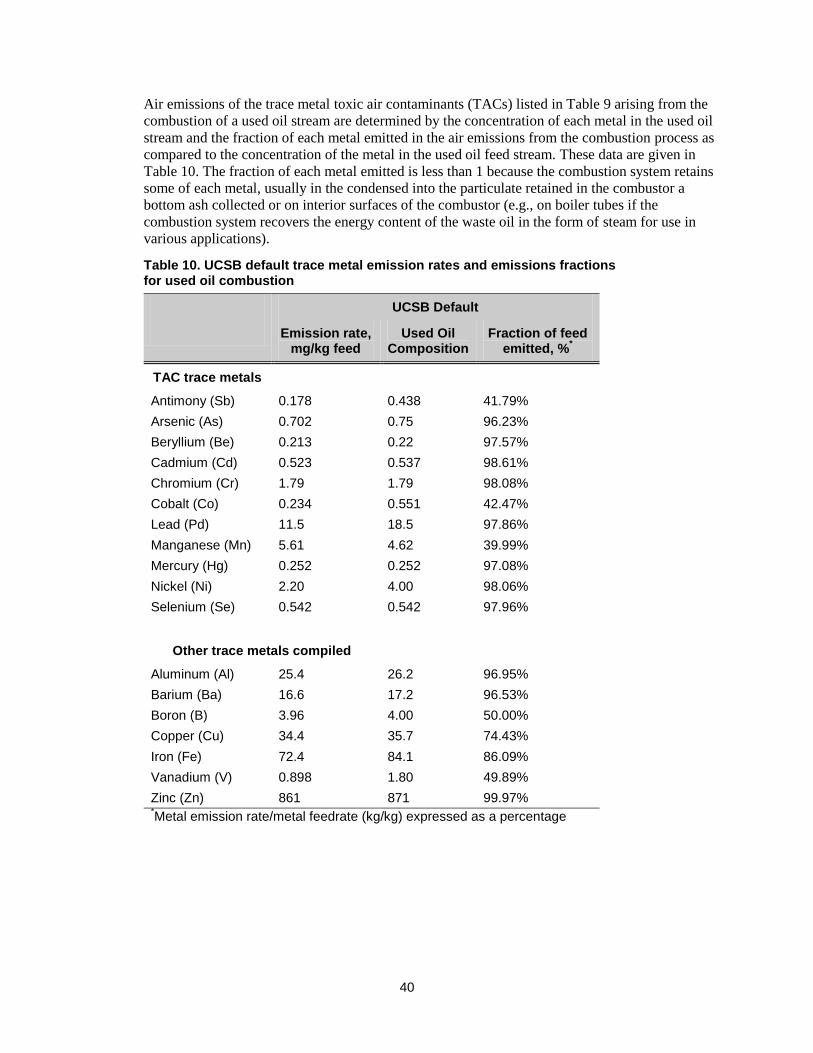
40
Air emissions of the trace metal toxic air contaminants (TACs) listed in Table 9 arising from the
combustion of a used oil stream are determined by the concentration of each metal in the used oil
stream and the fraction of each metal emitted in the air emissions from the combustion process as
compared to the concentration of the metal in the used oil feed stream. These data are given in
Table 10. The fraction of each metal emitted is less than 1 because the combustion system retains
some of each metal, usually in the condensed into the particulate retained in the combustor a
bottom ash collected or on interior surfaces of the combustor (e.g., on boiler tubes if the
combustion system recovers the energy content of the waste oil in the form of steam for use in
various applications).
Table 10. UCSB default trace metal emission rates and emissions fractions for used oil combustion
UCSB Default
Emission rate, mg/kg feed
Used Oil Composition
Fraction of feed emitted, %
*
TAC trace metals
Antimony (Sb) 0.178 0.438 41.79%
Arsenic (As) 0.702 0.75 96.23%
Beryllium (Be) 0.213 0.22 97.57%
Cadmium (Cd) 0.523 0.537 98.61%
Chromium (Cr) 1.79 1.79 98.08%
Cobalt (Co) 0.234 0.551 42.47%
Lead (Pd) 11.5 18.5 97.86%
Manganese (Mn) 5.61 4.62 39.99%
Mercury (Hg) 0.252 0.252 97.08%
Nickel (Ni) 2.20 4.00 98.06%
Selenium (Se) 0.542 0.542 97.96%
Other trace metals compiled
Aluminum (Al) 25.4 26.2 96.95%
Barium (Ba) 16.6 17.2 96.53%
Boron (B) 3.96 4.00 50.00%
Copper (Cu) 34.4 35.7 74.43%
Iron (Fe) 72.4 84.1 86.09%
Vanadium (V) 0.898 1.80 49.89%
Zinc (Zn) 861 871 99.97% *Metal emission rate/metal feedrate (kg/kg) expressed as a percentage

41
As the table shows, most (almost all) of the trace metal content in the feed waste oil fuel fed to a
combustor is emitted in the combustion gas emissions from the combustor. These waste oil
combustion systems rarely have emission controls that would capture particulate phase trace
metals (or vapor phase for that matter) so combustor emissions are the stack emissions to the
atmosphere. Notable exceptions to this observation are antimony (Sb), boron (B), cobalt (Co),
manganese (Mn), and vanadium (V). For these metals, emissions rates are 40 percent to 50
percent of the corresponding metal present in the waste oil feed. Presumably, a larger fraction of
these metals is emitted in the vapor phase, or retained by the combustion system (e.g., deposited
on boiler tubes or other combustor surfaces).

42
Table 11 summarizes the trace metal emission rates (mg/kg of metal in feed oil) for combustion
emissions of the UCSB default waste oil feed. Also shown in the table are the corresponding
emission rates for different fuel oil types taken from the EPA standard air emission factor
document, AP-42 (EPA 1995). As indicated in the table, for the toxic air contaminants (TAC)
trace metals, emission rates for the UCSB-defined default waste oil are comparable to those
emissions rates for waste oil taken from AP-42, though there are a few exceptions. TAC trace
metals emission rates for the UCSB-defined default waste oil are also greater (with a few
exceptions) than the AP-42 defined residual oil, which could be considered the proxy for heavy
fuel oil (HFO). This is likely due to the higher trace metal content of the used oil-based recycled
fuel oil (RFO). All the waste oil (UCSB study or AP-42) emission rates for toxic air contaminants
(TAC) trace metals are greater (sometimes significantly greater) than those from the AP-42
distillate fuel oil, as would be expected.
Comparisons between the TAC trace metal combustion emissions from the UCSB-defined, as
well as the AP-42, waste oil and those from the combustion of the AP-42 petroleum refining
residual fuel oil are mixed, though the emissions for the "other trace metals" (not TACs in Table
11) from combustion of the UCSB waste oil are uniformly much greater. In general, within the
range of variations in trace metal emission rates from combustion of fuel oils (waste or other), the
conclusion is that the default combustion model emission rates established for use by the UCSB
team in proceeding with a life cycle assessment (LCA) of waste oil management processes
incorporating waste oil combustion is as appropriate as any other defensible waste oil combustion
emissions characterization.
EMITTED TRACE METAL VALENCE STATE
What was done: UCSB reported the emissions from different combustion sources of
many trace metals (toxic air contaminants and others) with no valence state noted. For
others a valence state was reported, presumably for the most stable oxide of the
respective metal (combustion usually results in metal oxide emissions) The results are
in several Excel spreadsheet provided by UCSB.
Comment: The estimates of some valence states does not match the likely combustion
for some metals. This is the case for Cr and V.

43
Table 11. Comparison of UCSB default trace metal emission rates to AP-42 emission rates for liquid fuels
Emission rate, mg/kg feed*
UCSB Default waste
oil
AP-42
Waste oil
Residual fuel oil
Distillate fuel oil
TAC trace metals
Antimony (Sb) 0.178 0.544 0.635
Arsenic (As) 0.702 13.3 0.160 0.075
Beryllium (Be) 0.213 0.218 0.003 0.056
Cadmium (Cd) 0.523 1.12 0.048 0.056
Chromium (Cr) 1.79 2.42 0.102 0.056
Cobalt (Co) 0.234 0.025 0.728
Lead (Pd) 11.5 0.183 0.169
Manganese (Mn) 5.61 8.22 0.363 0.113
Mercury (Hg) 0.252 0.014 0.113
Nickel (Ni) 2.20 1.33 10.21 0.056
Selenium (Se) 0.542 0.083 0.281
Other trace metals compiled
Aluminum (Al) 25.4 0.311
Barium (Ba) 16.6 0.213 0.113
Boron (B) 3.96 0.095
Copper (Cu) 34.4 3.84
Iron (Fe) 72.4 3.52 0.075
Vanadium (V) 0.898
Zinc (Zn) 861 *Metal emission rate/metal feedrate (kg/kg) expressed as a percentage
Analysis Trace metal emissions from combustion sources, both for toxic air contaminants (TACs) and the
other metals noted in Table 10 and Table 11, are generally in the form of a stable oxide
compound of the metal (e.g., Sb2O3, As2O3, and so forth). Thus, the emitted valence state of the
metal is that corresponding to its stable oxide (Sb+3
, As+3
, and so forth). For most TAC trace
metals, the human health toxicity of the metal is presumed to be not significantly different among
its various valence states, thus a single metal composition is cited. However, for a few TAC trace
metals, the element's toxicity does depend on its valence state. The most notable example is
chromium (Cr).
Of the two most common naturally occurring chromium oxidation states, hexavalent chromium
(Cr+6
) is much more toxic (and carcinogenic) than trivalent chromium (Cr+3
). Chromium in the air

44
emissions from combustion sources are most likely as its most stable chromium oxide (Cr2O3) in
airborne particulate (trivalent Cr+3
), or as chromate (CrO42-
) or dichromate (Cr2O72-
) in aqueous
solution or associated with a cation such as sodium or magnesium (hexavalent Cr+6
). Chromate or
dichromate can be water pollutants produced in electrochemical processes, and can also be found
in combustion products, though usually at smaller fractions that Cr+3
. The hexavalent form is
much more toxic than the trivalent form. Thus, assuming air emissions of chromium to be Cr+6
can lead to highly misleading conclusions.
In the Final Report, UCSB states that “The California Air Resources Board assumes that
chromium emitted from combustion of used oil and other wastes to be ‘principally in the trivalent
state.’ ” UCSB adopts this assumption in the combustion model developed and employed to
estimate emissions in the life cycle assessment (LCA), and assumes that 80 percent of chromium
emissions are as trivalent and 20 percent hexavalent.
Table 12 shows some select trace metal emission data taken from the UCSB spreadsheets. The
data in the table illustrate a few disturbing items. Most noticeable is the wide difference between
the concentrations of the metals noted in the two oil products. These differences have a
significant effect on the LCA results reported (and to be reported) by UCSB is heavy fuel oil
(HFO) is the petroleum product to be replaced by waste oil-based recycled fuel oil (RFO), and its
replacement gives rise to the recycled fuel oil (RFO) environmental benefits (credits) in the LCA.
In particular, both Cr+3
and Cr+6
concentrations are reported in the table for RFO, but only noted
as Cr+6
for HFO. The Cr+6
fraction of total Cr (sum of +3 and +6) is 20 percent, in keeping with
the ARB recommendation. However, only Cr+6
emissions are shown for HFO combustion, which
is suspicious and likely misleading. The Cr measurement data comprising the Cr concentration
noted in Table 12 for HFO were most likely total Cr measurements. Thus, showing all Cr as Cr+6
is not in keeping with UCSB’s stated presumption, and overly conservative.
Table 12. Select reported emission factors from the December 2012 UCSB spreadsheets
Emissions per Fuel Energy
Content, g/MJ LHV
Pollutant RFO HFO
Cr+3
0.75 0
Cr+6
0.19 1,115
Cu+2
234 0
V+3
3,562 7
Similarly for vanadium (V), air emissions from the combustion of UO recycling products are
included in the UCSB composition sheets as trivalent V+3
. This presumes that the V emissions
from the combustion of used oil (UO) and its recycling products is V2O3. However, the most
common vanadium oxide is V2O5, in which the oxidation state of the V is V+5
. Only V2O5 has a
human health effects exposure limit. The Occupational Safety and Health Administration
(OSHA) has set an exposure limit in the workplace for worker exposure to V2O5 dust averaged
over an 8-hr workday for 40-hr/week of 0.05 mg/m3 (OSHA 2009). Thus, the UCSB assumption
that vanadium is emitted in the gaseous emissions from UO and it recycling products (RFO,
HFO, and MDO) as V+3
is misleading.

45
Displacement factors Displacement factors are the fractions of the petroleum product that is displaced by the used oil
processing product. For example recycled fuel oil (RFO) does not displace heavy fuel oil (HFO)
on a kg/kg basis because the RFO heat content MJ/kg) is less than that of HFO.
The life cycle assessment (LCA) model is set up to calculate the impacts of the used oil system
and those of the displaced products. The treatment of re-refined products from the used oil system
and substitute products is shown in Figure 2 and Figure 3. For the used oil system, products such
as re-refined base oil are treated as co-products with a displacement credit. The displacement
credit may be adjusted for economic factors. So, for example, 1 kg of base oil from re-refining
might displace 0.99 kg of base oil from virgin production based on supply/demand considerations
from the economic study.
UCSB should acknowledge the different treatment of products from the used oil system and
compared products from the displaced system. In the used oil system, co-products are potentially
adjusted with supply/demand displacement factors. However, no supply/demand effects for the
virgin oil production can be taken into account.
An alternative approach would have been to examine the virgin oil system with the same detail as
the used oil system since the value of displaced products is the key driver to the LCA study. Also
the source of emission factors for the PE analysis of oil refineries is different than the primary
data and other sources used in the used oil system. We recognize that the model configuration
cannot be change. UCSB should identify the limitations of using life cycle impact (LCI) data for
virgin base oil, MDO, and HFO production because the emission impacts are as large as those
from the used oil system.
It bears noting that no direct primary data from refineries were collected to validate U.S. EPA
statistics that have been used from literature, for example to validate that California refineries do
indeed use more energy. The UCSB report does not give a justification and it seems to be a
relevant difference that could be explained in terms of crude input and/or mix of technology. That
justification is missing.
In Appendix D where displacement modeling is described, was the completeness of the PE
models versus the LCI collected in the study for the combustion and other used oil management
practices reviewed to warrant that displacement factors are not missing emissions that are in the
used oil management model and vice versa. Perhaps a good way to review this is to look for the
main contributors per impact category and make sure the LCI data are covered in both parts of the
model. Has this check been performed, and if so, where is it reported?
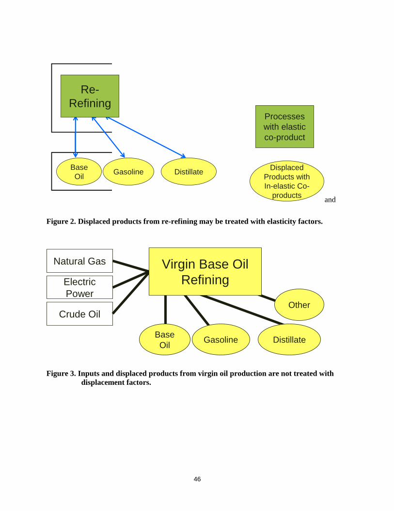
46
Used oil collection
Re-refining DistillationRFO
production
Displacedproduction
& combustion
Wastemanagement
Used oilgeneration
Displacedproduction
& use
Displacedproduction
& combustion
Displacedproduction
& use
Displacedproduction
& combustion
Combustionof RFO
Combustionof sec. fuels
Use of sec. products
Combustionof sec. fuels
Use of sec. products
Improperdisposal Hazardous
wasteincineration
Ancillary product
s
Contribution AnalysisContribution Analysis
Wastemanagement
Used oil processing & use of secondary products
Displaced production & use
Processes
with elastic
co-product
Displaced
Products with
In-elastic Co-
products
Base
OilGasoline Distillate
Re-
Refining
and
Figure 2. Displaced products from re-refining may be treated with elasticity factors.
Natural Gas
Electric
Power
Crude Oil
Base
OilGasoline Distillate
Other
Virgin Base Oil
Refining
Figure 3. Inputs and displaced products from virgin oil production are not treated with
displacement factors.

47
The UCSB approach to displacement to date can be summarized as follows:
What was done: Information reported by UCSB to date has focused on used oil (UO)
and its management processes quantities needed to be managed (e.g., generation rates
and quantities transferred in/out of state). Detailed displacement factors regarding the
quantities of petroleum products that may be displaced by UO and its management
process products have not been presented to date, though summary information has
been reported.
Comment: Details regarding displacement factors are needed for proper review of the
life cycle assessment (LCA). Such details are expected to discuss: rebound due to
marketplace price drops, the use technical energy equivalent displacement factors, and
the methods by which displacement factors are calculated.
In the UCSB Final Report, a detailed list of displacement relationships is provided at Table 9. The
last column indicates that displacement rates are based on MJ/MJ or kg/kg basis. Furthermore, for
some fuel products such as recycled fuel oil (RFO) or onsite combustion of used oil, a mix of No.
2 distillate, No. 6 residual and natural gas is used with identical proportion.
The UCSB report indicates (Section 4.3.6) that these assumptions are based on a consequential
approach (by referring to consequential LCA). Furthermore, the appendix D, which describes the
displacement model, includes several references to consequential procedure and LCA. However,
none of these procedures have really been used for determining the displaced products or the
displacement rates. In fact, the report indicates that a (appendix D, p. 289): “ 1:1 technical
displacement rate is assumed in the Used Oil LCA model” and “where a product has the potential
to displace several primary products, an equal split between the primary products is assumed.”
These assumptions are essentially attributional approaches because they do not consider
relationships such as price elasticity, joint production constraints or impact on marginal processes
between used oil management system co-products and displaced products. In other words, the
study assumes that additional production of this used oil co-products can always be absorbed by
the market and they will lead to direct substitution of equivalent products without any
consequences.
Furthermore, the refinery model presented in the PE’s document (November 2012) is a purely
attributional life cycle impact (LCI) model. This means that refinery co-products are essentially
independent from each other and their production output can vary independently (no joint
production constraints).
Take note that system expansion should not be considered a de facto consequential approach. As
mentioned in the ILCD Handbook (General guide for LCA, March 2010, section 6.5.2, p. 77),
“Substitution is also applicable for attributional modeling that is interested to include existing
interactions with other systems.”
Therefore, the only real consequential approach in this study is the Direct Impacts Model
developed by ICF International which is used for determining the reference flow for the 10
scenarios.

48
The actual description of the life cycle impact (LCI) model creates an ambiguity about the
modelling approach. The authors should avoid this ambiguity and be clear about what is really
consequential modelling and what is not. This is especially important because this study is for
macro-level decision support with a long term perspective and direct and indirect consequences
on the petrochemical sector could be significant. These consequences are not necessarily captured
by this model and this should be presented as a limit of this study.

49
Impact Analysis
What was done: UCSB defined suite of impact indicators (greenhouse gas (GHG)
emissions, smog formation, etc.), calculated impact indicators using TRACI 2.0 (EPA).
Combustion of UO recycling products (RFO, MDO+rerefined) beneficial (net negative
impact) when weighed against avoided burden of petroleum products replaced for all
but two indicators (eutrophication, human health air criteria).
Comment: Air emissions end point impacts seem appropriate: GHG emissions, air
acidification captures SO2, NOx emissions, smog captures NOx, VOC emissions, cancer
cases captures diesel PM emissions, air criteria captures PM10 emissions)
Eutrophication captures aquatic impacts.
More needs to be said about the interpretation of eutrophication example. Because eutrophication
is place specific, and the disposition route is key in determining net environmental
burden/benefit, can it be determined in any way where the eutrophication takes place? Is it an
impaired body or water? Is it a protected one? One can envision a scenario where the study’s
interpretation of a net benefit can actually increase the burden on a particular body of water?
Likewise, something seen as a net burden might largely impact an area where eutrophication is
already present as a problem. It is recognized that TRACI 2.0 is not site specific, but because
eutrophication has impaired more than 50 percent of rivers, it would be good to at least have
some better context to interpret reported results.
Phosphorous has bigger impacts to freshwater lakes, while nitrogen has bigger impacts to coastal
environments. Can any conclusions be drawn from the constituents of the kg N eq metric and its
actual impact on the particular water systems where the impacts occur? Any differentiation
between nitrogen and phosphorous induced eutrophication is not described in the Final Report.
A better explanation for ecotoxicity is warranted. Unlike the other impact metrics, this one is not
intuitive and it is not clear what the metric conveys, aside from its relative significance compared
to other scenarios and sensitivities. The implications of the toxicity findings remain difficult to
interpret in the Final Report.
Nevertheless the impact categories developed for the used oil life cycle assessment (LCA) seem
comprehensive, with the exception of the aquatic impacts. While eutrophication does capture
some aquatic impacts (it should be noted that eutrophication also applies to terrestrial systems), it
does not capture all or the most relevant aquatic impacts from used motor oil processing or
improper disposal. Eutrophication as an impact category is largely driven by nitrogen,
phosphorous, and biological oxygen demand from organic materials. However, there are more
relevant impact categories for impacts to aquatic ecosystems. Both freshwater aquatic ecotoxicity
and marine aquatic ecotoxicity should also be used to assess aquatic impacts as the may have very
different results than eutrophication. This is particularly near the San Francisco Bay where the
proposed re-refining facility will most likely release effluents. However, it appears that the
TRACI 2.0 model does not make this differentiation. Perhaps a summary of how the aggregated
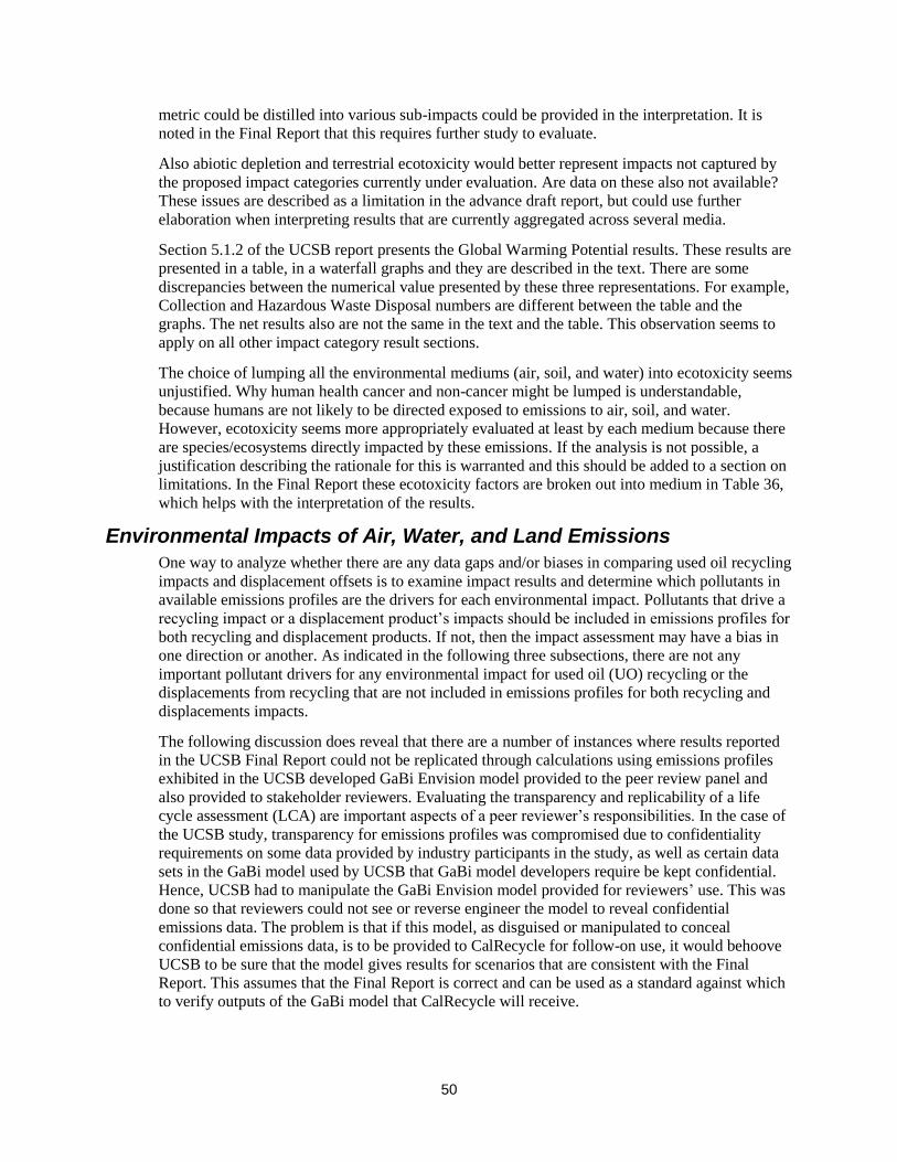
50
metric could be distilled into various sub-impacts could be provided in the interpretation. It is
noted in the Final Report that this requires further study to evaluate.
Also abiotic depletion and terrestrial ecotoxicity would better represent impacts not captured by
the proposed impact categories currently under evaluation. Are data on these also not available?
These issues are described as a limitation in the advance draft report, but could use further
elaboration when interpreting results that are currently aggregated across several media.
Section 5.1.2 of the UCSB report presents the Global Warming Potential results. These results are
presented in a table, in a waterfall graphs and they are described in the text. There are some
discrepancies between the numerical value presented by these three representations. For example,
Collection and Hazardous Waste Disposal numbers are different between the table and the
graphs. The net results also are not the same in the text and the table. This observation seems to
apply on all other impact category result sections.
The choice of lumping all the environmental mediums (air, soil, and water) into ecotoxicity seems
unjustified. Why human health cancer and non-cancer might be lumped is understandable,
because humans are not likely to be directed exposed to emissions to air, soil, and water.
However, ecotoxicity seems more appropriately evaluated at least by each medium because there
are species/ecosystems directly impacted by these emissions. If the analysis is not possible, a
justification describing the rationale for this is warranted and this should be added to a section on
limitations. In the Final Report these ecotoxicity factors are broken out into medium in Table 36,
which helps with the interpretation of the results.
Environmental Impacts of Air, Water, and Land Emissions
One way to analyze whether there are any data gaps and/or biases in comparing used oil recycling
impacts and displacement offsets is to examine impact results and determine which pollutants in
available emissions profiles are the drivers for each environmental impact. Pollutants that drive a
recycling impact or a displacement product’s impacts should be included in emissions profiles for
both recycling and displacement products. If not, then the impact assessment may have a bias in
one direction or another. As indicated in the following three subsections, there are not any
important pollutant drivers for any environmental impact for used oil (UO) recycling or the
displacements from recycling that are not included in emissions profiles for both recycling and
displacements impacts.
The following discussion does reveal that there are a number of instances where results reported
in the UCSB Final Report could not be replicated through calculations using emissions profiles
exhibited in the UCSB developed GaBi Envision model provided to the peer review panel and
also provided to stakeholder reviewers. Evaluating the transparency and replicability of a life
cycle assessment (LCA) are important aspects of a peer reviewer’s responsibilities. In the case of
the UCSB study, transparency for emissions profiles was compromised due to confidentiality
requirements on some data provided by industry participants in the study, as well as certain data
sets in the GaBi model used by UCSB that GaBi model developers require be kept confidential.
Hence, UCSB had to manipulate the GaBi Envision model provided for reviewers’ use. This was
done so that reviewers could not see or reverse engineer the model to reveal confidential
emissions data. The problem is that if this model, as disguised or manipulated to conceal
confidential emissions data, is to be provided to CalRecycle for follow-on use, it would behoove
UCSB to be sure that the model gives results for scenarios that are consistent with the Final
Report. This assumes that the Final Report is correct and can be used as a standard against which
to verify outputs of the GaBi model that CalRecycle will receive.

51
UO Recycled to RFO
Table 13 provides such a comparison for recycled fuel oil (RFO). The pollutant drivers for
impacts from used oil (UO) processing into RFO and combustion of RFO are shown in the
columns labeled RFO. Drivers for avoided life cycle impacts from displacement of diesel, heavy
fuel oil (HFO), and natural gas are shown in columns labeled Displacements. Percentages in each
column indicate the proportion of a specific environmental impact that is caused by a specific
pollutant. As can be seen from the percentages shown in each column, surprisingly few
pollutants, less than ten and sometimes only one, actually cause most of any given impact. In
addition, the few pollutants driving each particular impact tend to be different for different
impacts. Furthermore, fewer than 20 pollutants cause almost all of every environmental impact
tabulated in Table 13, as well as Table 14 and Table 15 discussed below.
The displacement life cycle profiles include production of diesel, HFO and natural gas in addition
to combustion emissions. The percentages in each column indicate the proportion of each
environmental impact that are caused by a particular pollutant based on emissions profiles
provided in the GaBi Envision Used Oil Management 1_59 Review Revised Final 2013_07_13
model provided by UCSB to the reviewers. Ignoring exports from California, one kilogram (kg)
of UO available for recycling can be processed into 0.91 kg RFO. The UCSB developed Envision
model estimates that each 0.91 kg of RFO combustion displaces production and combustion of
approximately 0.24 kg No. 2 distillate oil (diesel), 0.25 kg No. 6 residual oil (HFO), and 0.21 kg
natural gas.
The RFO combustion emissions profile contains under 35 pollutants, with most having
environmental impact characterization factors that are included in TRACI 2.0. By contrast the
RFO processing emissions profile and the diesel, HFO, and natural gas combined production and
combustion emissions profiles cover over 325 pollutants, of which about half are characterized in
TRACI 2.0. Total RFO combustion impacts tend to be two or more orders of magnitude larger
than processing impacts, except for human health—cancer for which combustion impacts are
many more than two times higher than reprocessing, and ecotoxicity for which RFO processing
impacts are many times larger than from combustion.
Comparisons in Table 13 do not reveal any cases where a pollutant that causes a substantial
portion of an environmental impact for RFO processing and combustion is not covered by the
emissions profile for diesel, HFO, and natural gas production and combustion, or vice versa.
However, the table does indicate that there are pollutants for which the RFO impact proportion
differs substantially from the displaced diesel, HFO and natural gas impact proportion. Pollutants
causing environmental impacts for which these RFO versus Displacement proportion differences
are large are highlighted in Table 13.
The sulfur content of diesel or HFO versus RFO may be the cause of the disparities for sulfur
dioxide and PM2.5 shown for human health respiratory impacts from criteria air pollutants. That
is, sulfur dioxide accounts for 74 percent of human respiratory impacts for displaced fuels, but
only 31 percent for RFO. PM2.5 accounts for 48 percent of RFO impacts, and just 13 percent of
displacements impacts
For human non-cancers and ecotoxicity, zinc emissions drive more than 95 percent of the
environmental impact for RFO. However, zinc does not dominate the emissions avoided by RFO
displacements because arsenic, barium, copper, and silver also drive virgin fuel production and
combustion human non-cancer and ecotoxicity impacts. For human cancers, hexavalent
chromium, mercury, lead, and arsenic, in that order, cause most of RFO’s impact. Impacts
avoided by RFO displacements flow from arsenic, nickel, mercury, and hexavalent chromium.

52
Table 13. Impact assessment for RFO
RFO Displacements RFO Displacements RFO Displacements RFO Displacements RFO Displacements RFO Displacements RFO Displacements RFO Displacements RFO Displacements
Carbon Dioxide 99.6% 93.5%
Methane 0.1% 6.3% 0.0% 0.1%
Nitrous Oxide 0.3% 0.2%
Sulfur Dioxide 31.1% 73.8% 65.0% 69.3%
Nitrogen Oxides 3.2% 6.4% 32.7% 30.0% 22.0% 91.0% 99.3% 99.4%
Hydrogen Chloride 2.3% 0.3%
Hydrogen Sulfide 0.0% 0.2%
PM10 17.4% 6.9%
PM2.5 48.3% 12.8%
Nitrogen 0.0% 6.5%
COD 8.0% 62.6%
Phosphate 0.0% 14.3%
Phosphorus 78.0% 2.3% 59.9% 0.4%
BOD 4.2% 8.5%
Ammonia 0.0% 0.3% 1.6% 5.1%
Ammonium 10.1% 0.4%
Nitrate 16.2% 8.7%
Hydrogen Fluoride 0.0% 0.2%
Isoprene 0.0% 0.1%
n-Butane 0.0% 0.1%
Propane 0.0% 0.2%
VOCs 0.6% 0.0%
Phenol 0.0% 0.4%
Anthracene 0.0% 0.1%
Barium(II) 0.0% 6.4% 0.0% 19.8%
Beryllium(II) 0.0% 0.4%
Silver(I) 0.1% 0.2% 0.3% 15.9%
Copper(II) 1.3% 37.0%
Arsenic(V) 7.1% 40.7% 0.1% 23.5% 0.1% 6.4%
Nickel(II) 2.2% 21.8% 0.0% 6.3%
Zinc(II) 97.5% 42.3% 95.6% 12.4%
Mercury(II) 27.4% 18.0% 0.5% 16.7% 0.0% 0.1%
Chromium(III) 0.0% 0.4%
Chromium(VI) 48.1% 14.8% 0.1% 0.4%
2,3,7,8 - TCDD 0.0% 0.1%
Lead(II) 10.0% 2.9% 0.5% 7.9% 0.0% 0.1%
Antimony (III) 0.0% 0.0%
Cobalt (II) 0.1% 0.0%
Cadmium(II) 5.2% 1.3% 0.2% 2.6% 0.0% 0.6%
Molybdenum 1.0% 0.0%
Thallium 2.5% 0.0%
Benzene 0.0% 0.3% 0.0% 0.0%
Totals 100.0% 100.0% 100.0% 100.0% 99.9% 99.8% 99.9% 100.0% 100.0% 99.9% 100.0% 100.0% 100.0% 100.0% 100.0% 99.9% 99.9% 99.9%
Impacts/kg used oil recycled to RFO 2.75E+00 -3.21E+00 2.32E-03 -1.65E-03 2.08E-10 -3.01E-10 1.46E-06 -3.84E-08 3.39E-01 -5.36E-01 5.57E-04 -1.95E-04 8.44E-07 -1.85E-05 6.90E-02 -1.00E-01 1.58E+00 -1.94E-01
Net Impact
5.58E-04 -2.14E-04 } Air + water eutrophication
} in above table
Final Report Extreme RFO Scenario Results
Impacts/kg used oil recycled to RFO 2.75E+00 -3.20E+00 2.10E-03 -1.54E-03 3.17E-10 -4.11E-10 1.01E-06 -3.35E-08 3.10E-01 -4.97E-01 5.58E-04 -2.07E-04 6.91E-02 -1.00E-01 1.10E+00 -2.67E-01
Net Impact
HH - Cancers HH - Non-cancers
Pollutants
Percent of Environmental Impact Caused by Indicated Pollutant for RFO Processing and Combustion Versus Virgin Oil Production and Combustion Displacements in California
Climate Change AcidificationHH - Criteria Air Eutrophication - Air Eutrophication - Water Smog Ecotoxicity
1.42E-06
cases
-4.51E-01 5.62E-04 -9.39E-11 9.72E-07
-4.55E-01 6.74E-04 -9.29E-11
kg CO2 eq kg PM10 eq cases
-1.87E-01 3.51E-04
-1.97E-01
kg H+ moles eq
3.62E-04
kg N eq
3.44E-04
-1.77E-05
kg N eq
-3.11E-02 8.37E-01
-3.10E-02
kg O3 eq
1.38E+00
PAF.m3.day.kg-1

53
There also are substantial differences in the proportions of RFO versus displacements impacts for
particular pollutants for eutrophication. RFO eutrophication of air is 78 percent from phosphorous
and 22 percent from NOx emissions. In contrast, NOx constitutes 91 percent and phosphorous
just 2 percent of eutrophication of air avoided by RFO displacements. For eutrophication of
water, phosphorous accounts for 60 percent of RFO impacts, but chemical oxygen demand causes
63 percent of avoided impacts.
For climate change, acidification, and smog there are no substantial differences between drivers
of RFO and RFO displacements impacts.
Rows in the bottom section of Table 12 under the heading “Impacts/kg used oil recycling to
RFO” and rows below the table under the heading “Final Report Extreme RFO Scenario Results”
show net impacts of recycling one kilogram used oil into RFO in California as computed from the
GaBi Envision model provided to reviewers by UCSB and as reported in UCSB’s Final Report.
For climate change, human health—cancers, acidification, eutrophication (air plus water), and
smog, the two sets of net impacts estimates are quite close. Given that UCSB had to populate the
GaBi Envision model in a way that concealed confidential information provided to UCSB for
their LCA, and given the aggregated and rounded numbers for impacts and used oil quantities
shown in the Final Report, such differences are not problematic.
However, the differences between GaBi Envision model results and report results for human
health—criteria air and cancer and for ecotoxicity are not so easy to overlook. The approximately
15% difference for human health—criteria air impacts may be caused by some disparities in
classifying particulate emissions as PM2.5 or PM10, as has been discussed by UCSB with the
peer review panel. The differences between reviewer’s Envision model calculations and UCSB’s
Final Report for human health— non-cancers and for ecotoxicity are greater than 30 percent.
Since these two impacts are driven by metals emissions, as shown in Table 13, there may be a
problem with the metals emissions populating the extremes Envision model scenarios. Whatever
the cause, if this model, as disguised or manipulated to conceal confidential emissions data, is to
be provided to CalRecycle for follow-on use, it would behoove UCSB to be sure that the model
gives results for scenarios that are consistent with the Final Report, assuming that the Final
Report is correct and can be used to verify outputs of the GaBi model that CalRecycle will
receive.
UO Recycled to Re-refined Lubricating Oil
Table 14 provides a similar set of comparisons for recycled lubricating oil that is re-refined for
use again as lubricating oil. In this case, the displaced products are virgin lubricating oils,
bitumen (an asphalt component), ethylene glycol (an antifreeze component), and several minor
co-product fuels. Processing one kilogram of used oil into re-refined lubricating/base oil (RRBO)
yields 0.64 kg RRBO, 0.14 kg bitumen replacement, 0.08 kg fuels, and .001 kg ethylene glycol.
Pollutant emissions from processing used oil to make a portion of it usable again as base
lubricating oil, yielding the two co-products bitumen and ethylene glycol and the light fuel co-
products along the way, are shown in columns labeled RRBO. That column also accounts for
combustion of the light fuel co-products. Emissions reductions from avoided production of virgin
lube oil, bitumen, and ethylene glycol, as well as from avoided production and combustion of
displaced fuels are tabulated in columns labeled Displacements.

54
Table 14. Impact assessment for re-refined lubricating oil
RRBO Displacements RRBO Displacements RRBO Displacements RRBO Displacements RRBO Displacements RRBO Displacements RRBO Displacements RRBO Displacements RRBO Displacements
Carbon Dioxide 93.0% 88.4%
Methane 6.9% 11.3% 0.2% 0.2%
Nitrous Oxide 0.2% 0.3%
Sulfur Dioxide 94.7% 63.8% 86.8% 75.3%
Nitrogen Oxides 2.6% 4.0% 11.8% 23.1% 78.2% 88.9% 93.9% 97.4%
Hydrogen Chloride 0.4% 0.3%
Hydrogen Fluoride 0.1% 0.1%
Hydrogen Sulfide 0.8% 0.8%
PM10 1.1% 16.7%
PM2.5 1.6% 15.5%
Nitrogen 20.6% 9.3% 4.4% 43.0%
COD 19.2% 24.0%
Phosphate 3.6% 18.3%
Phosphorus 0.4% 0.3% 33.9% 0.3%
BOD 11.0% 6.0%
Ammonia 0.1% 0.3% 0.7% 1.5% 10.5% 5.8%
Ammonium 6.5% 0.2%
Nitrate 10.9% 2.4%
Carbon Monoxide 0.0% 0.1%
n-Butane 0.0% 0.2%
Isoprene 2.6% 0.8%
Pentane 0.0% 0.1%
Ethane 0.0% 0.1%
VOCs 2.9% 0.6%
Propane 0.0% 0.5%
Barium(II) 59.8% 23.0% 49.0% 37.4%
Silver(I) 1.5% 0.9% 44.2% 32.4%
Copper(II) 1.2% 16.7%
Arsenic(V) 19.3% 67.1% 14.0% 30.3% 1.1% 4.4%
Nickel(II) 2.4% 8.6% 0.4% 1.7%
Zinc(II) 10.5% 29.0% 3.5% 6.1%
Mercury(II) 9.9% 15.6% 11.6% 11.2%
Chromium(III) 0.1% 0.2%
Chromium(VI) 65.4% 4.3% 0.3% 0.0%
2,3,7,8 - TCDD 0.1% 0.1%
Lead(II) 0.4% 2.2% 1.2% 4.8%
Cadmium(II) 0.4% 0.4% 1.1% 0.7% 0.0% 0.4%
Phenol 0.0% 0.3%
Benzene 2.0% 1.4% 0.2% 0.0%
Formaldhyde 0.0% 0.1%
Totals 100.0% 100.0% 100.0% 100.0% 100.0% 99.9% 99.8% 99.9% 100.0% 100.0% 100.0% 100.0% 100.0% 100.0% 99.9% 100.0% 99.9% 99.7%
Net Impact
5.73E-05 -1.37E-04 } Air + water eutrophication
} in above table
Review Report Extreme ReRe Scenario Results
Impacts/kg used oil recycled to RFO 5.07E-01 -1.08E+00 3.66E-04 -1.13E-03 3.39E-10 -2.80E-10 1.65E-08 -4.17E-08 1.19E-01 -2.60E-01 5.18E-05 -1.28E-04 8.99E-03 -3.26E-02 3.04E-01 -4.16E-01
Net Impact
kg N eq kg N eq kg O3 eq PAF.m3.day.kg-1kg CO2 eq kg PM10 eq cases cases kg H+ moles eq
1.08E-02 -3.91E-02 3.40E-01 -4.04E-01
-5.52E-01 -6.14E-04 -8.04E-11 -2.42E-08 -1.28E-01 -5.33E-05 -2.60E-05 -2.83E-02 -6.38E-02
-2.66E-01 2.31E-05 -7.64E-05 3.42E-05 -6.02E-051.77E-10 -2.57E-10 1.79E-08 -4.22E-08 1.38E-01Impacts/kg used oil recycled to ReRe 5.77E-01 -1.13E+00 4.15E-04 -1.03E-03
HH - Cancers HH - Non-cancers
Pollutants
Percent of Environmental Impact Caused by Indicated Pollutant for Processing and Production of Re-refined Base Oil (RRBO) and Co-Products Versus Virgin Oil and Co-Product Displacements in California
Climate Change AcidificationHH - Criteria Air Eutrophication - Air Eutrophication - Water Smog Ecotoxicity
-2.36E-02 -1.12E-01
-7.94E-05
-5.73E-01 -7.66E-04 5.99E-11 -2.52E-08 -1.41E-01 -7.66E-05

55
Comparisons in Table 14 do not reveal any cases where a pollutant that causes a substantial portion of an
environmental impact for used oil (UO) recycling into re-refined base oil (RRBO) and co-products is not
covered by the emissions profile for displaced products and fuels. In addition, the table indicates that there
are only five pollutant-impact combinations for which the RRBO impact proportion differs substantially
from that for displaced products and fuels. Pollutants causing environmental impacts for which these
RRBO versus Displacement proportion differences are large are highlighted in Table 14.
For sulfur dioxide, Table 14 for criteria air pollutants indicates that sulfur dioxide accounts for 95 percent
of this human health impact from processing and production of RRBO and co-products. At the same time
this pollutant explains 64 percent of displacement impacts. The RRBO compared with Displacements
proportions for arsenic and hexavalent chromium are substantially different for human cancers. Lastly, the
nitrogen and phosphorous proportions are substantially different between RRBO and Displacements for
eutrophication of water impacts.
The comparison between GaBI Envision model extremes scenario and the UCSB Final Report estimates of
impacts per kilogram of used oil re-refined into new lube oil is more troubling for RRBO than for recycled
fuel oil (RFO). As indicated in Table 14, the two sets of estimates are within 10 percent of each other only
for climate change, human non-cancers and acidification. Smog estimates differ by more than 15 percent,
criteria air estimates differ by about 25 percent, and eutrophication estimates differ by more than 40
percent. The ecotoxicity impact estimates differ by 75 percent. Lastly, the impact estimates for human
cancers have different signs—i.e., the Envision model for the extreme re-refining scenario shows re-
refining having a net positive impact by reducing the potential for human cancers, while the UCSB Final
Report estimates that re-refining increases the potential for human cancers.
UO Recycled to Marine Distillate Oil
Table 15 provides comparisons for recycled lubricating oil that is distilled into a marine distillate oil
(MDO) and co-products. Processing one kilogram of used oil into this marine fuel yields 0.52 kg MDO,
0.31kg bitumen, and less than 0.01 kg light ends used as fuels.
As was the case for RFO in Table 13 and RRBO in Table 14, comparisons in Table 15 do not reveal any
cases where a pollutant that causes a substantial portion of an environmental impact for UO recycling into
MDO and co-products is not covered by the emissions profile for displaced products and fuels and vice
versa. Moreover, the table indicates that there are eight pollutant-impact combinations for which the MDO
impact proportion differs substantially from the displaced products and fuels impact proportion. Pollutants
causing environmental impacts for which these MDO versus Displacement proportion differences are large
are highlighted in Table 15.
At 61 percent, chemical oxygen demand (COD) dominates water eutrophication from MDO displacements,
whereas phosphorous provides 45 percent of MDO processing and combustion impacts compared with just
17 percent for COD. Barium and silver are important for MDO processing and combustion ecotoxicity
impacts, but are less than half as significant for ecotoxicity avoided by MDO displacements. Silver is a
driver of cancer and non-cancer impact potential for product and fuel production and combustion
displacements. Mercury is dominant for cancer and non-cancer impacts from MDO processing and
combustion.
The comparison between UCSB Final Report and reviewer calculations using the UCSB developed GaBI
Envision extreme MDO model estimates of environmental impacts per kilogram of used oil recycled to
MDO shows that the two sets of estimates are within 5 percent for climate, acidification, eutrophication,
and smog. Human cancer, criteria air pollutant, and eutrophication impacts differ by less than 15 percent.
Non-cancer and ecotoxicity have opposite signs in the two sets of estimates, with Envision showing a
negative net impact in both cases and the UCSB Final Report estimating a positive net environmental
benefit.

56
Table 15. Impact assessment for MDO
MDO Displacements MDO Displacements MDO Displacements MDO Displacements MDO Displacements MDO Displacements MDO Displacements MDO Displacements MDO Displacements
Carbon Dioxide 97.1% 93.7%
Methane 1.0% 4.6%
Nitrous Oxide 1.9% 1.7%
Sulfur Dioxide 23.3% 26.1% 15.6% 18.2%
Nitrogen Oxides 25.4% 23.6% 84.3% 81.5% 99.3% 98.9% 99.3% 99.3%
Hydrogen Chloride 0.1% 0.1%
Hydrogen Sulfide 0.0% 0.1%
PM10 6.7% 8.8%
PM2.5 44.6% 41.5%
Nitrogen 0.4% 0.7%
COD 16.8% 61.2%
Phosphate 0.0% 14.9%
Phosphorus 0.3% 0.3% 44.8% 0.4%
BOD 9.6% 8.2%
Ammonia 0.0% 0.0% 8.4% 5.5%
Ammonium 7.8% 0.5%
Nitrate 12.6% 9.3%
VOCs 0.6% 0.6%
Phenol 0.0% 0.5%
Anthracene 0.0% 0.1%
Barium(II) 6.9% 3.3% 40.4% 18.6%
Beryllium(II) 0.0% 0.2% 0.2% 1.3% 0.0% 0.1%
Silver(I) 2.3% 0.1% 39.1% 14.0%
Copper(II) 3.2% 32.5%
Arsenic(V) 11.1% 31.4% 6.2% 23.7% 2.7% 11.0%
Nickel(II) 1.2% 4.2% 0.7% 3.9%
Zinc(II) 23.6% 31.4% 11.8% 14.9%
Mercury(II) 54.8% 20.9% 52.4% 26.0% 0.3% 0.2%
Chromium(III) 0.1% 0.5%
Chromium(VI) 29.1% 38.7% 0.9% 1.5%
2,3,7,8 - TCDD
Lead(II) 1.5% 2.5% 4.2% 9.1% 0.0% 0.1%
Antimony (III) 0.2% 0.1% 0.2% 0.1%
Cobalt (II) 0.2% 0.1%
Cadmium(II) 1.9% 1.9% 3.9% 5.1% 0.2% 0.9%
Selenium(IV) 0.3% 0.8%
Benzene 0.3% 0.1%
Totals 100.0% 100.0% 100.0% 100.0% 99.9% 99.9% 100.0% 100.0% 100.0% 99.9% 100.0% 100.0% 100.0% 100.0% 100.0% 99.9% 99.9% 99.9%
Impacts/kg used oil recycled to RFO 1.83E+00 -2.10E+00 2.16E-03 -2.44E-03 6.07E-10 -7.56E-10 7.52E-08 -7.19E-08 9.83E-01 -1.07E+00 9.23E-04 -9.71E-04 2.08E-05 -1.51E-05 5.16E-01 -5.41E-01 2.00E-01 -1.95E-01
Net Impact
9.44E-04 -9.86E-04 } Air + water eutrophication
} in above table
Review Report Extreme MDO Scenario Results
Impacts/kg used oil recycled to RFO 1.77E+00 -2.03E+00 2.87E-03 -3.19E-03 1.54E-09 -1.71E-09 7.18E-08 -7.27E-08 9.50E-01 -1.03E+00 9.08E-04 -9.49E-04 4.98E-01 -5.23E-01 2.07E-01 -2.21E-01
Net Impact -7.87E-02 -4.10E-05 -1.37E-02-3.17E-04 -1.70E-10 -8.68E-10 -2.45E-02
4.68E-035.74E-06 -2.50E-02
HH - Cancers HH - Non-cancers
Pollutants
Percent of Environmental Impact Caused by Indicated Pollutant for Processing Used Oil into MDO and Co-Products and MDO Combustion Versus Virgin Oil Production of Marine Fuel and Co-Products and Marine Fuel Combustion Displacements in California
Climate Change AcidificationHH - Criteria Air Eutrophication - Air Eutrophication - Water Smog Ecotoxicity
-2.64E-01
PAF.m3.day.kg-1kg O3 eqkg N eqkg N eqkg H+ moles eq
-4.20E-05
-2.74E-01
kg CO2 eq
3.23E-09
cases
-1.49E-10
cases
-2.78E-04
kg PM10 eq
-8.24E-02 -4.77E-05

57
Uncertainties
Also, as important as concerns regarding the life cycle assessment (LCA) comparisons of
products made from recycled used oil (UO) and the virgin products displaced by those recycled-
content products, is the general issue of data uncertainties. These may include:
Use of “canned” GaBi emissions profiles that may or may not be representative of actual
practices in California.
Exclusion of impact contributions from more than 50 specific pollutants included in
emissions profiles that are not covered by TRACI 2.0 impact characterizations.
Exclusions of impacts from pollutants included in broad categories used in the inventories of
emissions profiles, such as, among others, aldehydes, alkanes, alkenes, polycyclic
hydrocarbons, non-methane hydrocarbons, and non-specific dioxins.
Exclusions of radioactive emissions activity levels from human and ecosystem health impact
characterizations provided by TRACI 2.0.
Sensitivity Analysis
Reviewer comments on the sensitivity analysis presented in the Final Report include the
following:
Tested and default parameters for the displacement assumptions regarding recycled fuel oil
(RFO) sensitivity analysis are not presented.
In Section 6.2.2 of the Final Report, the IMPACT 2002+ ecotoxicity categories have not been
considered in this sensitivity analysis. Is there any reason for this?
In section 6.2.3 of the Final Report, the text incorrectly indicates that “Using TRACI 2.0,
marine distillate oil (MDO) and ReRe are shown to have lower or negative environmental
impacts versus RFO.” In fact, this is only true for air ecotoxicity. Water and soil ecotoxicity
results show the exact opposite.
The text describing Figures 52 and 53 indicates: “Used oil composition can be seen to have
very little effect on CML marine toxicity and, strangely, ReCiPe freshwater toxicity.” In
general, it would be expected that a LCA practitioner can provide a precise explanation for
this type of observation, at least for the inventory flows and characterization factors that are
behind this result.
The thorough assessment of the toxicity sensitivity is definitely a welcomed addition to this the
final version of the UCSB report. The testing of different LCIA methods and the most sensitive
parameters clearly shows all the possible range of variability for results and conclusions.
However, the complexity and number of analyses presented in the sensitivity analysis section of
the report make it difficult for the reader to draw strong and useful conclusions. There is really a
need for a wrap up of the main conclusions that goes beyond the general statement provided in
Section 6.2.5 of the Final Report. In other words, are there strong conclusions that arise from all
the variability observed for the toxicity categories? Alternatively, should we assume that results
are too uncertain to consider the results from this environmental issue in final decision-making?
An option for summarizing all this information would be to provide a ranking table with a color
code to easily highlight consistent trends for each scenario.

58
Regional Analysis
The lack of any regional analysis within the state of California makes interpreting these results
very difficult. It will be difficult for policy-makers to draw conclusions about the distribution of
impacts within the state. This is generally the case with life cycle assessments (LCAs), but
someone with some familiarity of where impacts would occur in the extreme scenarios should be
able to assess generally where impacts will occur and if they will occur near impaired waterways,
out-of-compliance air sheds, etc. The research team and stakeholders should come up with some
generalizations for how impacts would be distributed across the state. These limitations are not
described in the limitations section of the report.
Interpretation of Results
In general, the results, conclusions, and recommendations for future work are not clearly
indicated and that makes the UCSB report of a lesser value than it can have. The researchers
should spend more time on the conclusions section and interpretation of results for a non-
technical audience. There is not much to go on for policy makers with so few words that are used
in the current report, and that is one of the goals of the LCA.
In section 6.1, it is stated that many results are driven by one or more impacts. More discussion is
needed on the certainty of the impacts, are they measured, estimated, calculated, from primary
sources, or literature? The quality of the values of the impact is relevant information for the
interpretation and can guide as to which impacts can be best used now for recommendations, and
which should be researched more to be more certain about the aggregated impact and hence
differences between the different scenarios. These qualifications will improve the ability for
readers to interpret the results.
Section 6.2.6 should have a short (one-sentence) explanation for why there are no significant
changes in any scenario.
Section 6.5 on conclusions seems far too short. There are many conclusions that can be drawn.
For example, the results in 6.1 can be tied to the sensitivities in the following sections. More
conclusions should be added as they pertain to the LCA and not the policy recommendations.
A section on recommendations for future research should be added: what should be developed in
the coming years to be able to address some of the difficult parts where you had to make the
biggest assumptions?
A section on limitations should be added to the conclusions section. These limitations can be
directly related to recommendation for future research. The LCA team’s expertise will be very
helpful in determining future research directions, data needs, etc.
The LCA results in the advanced draft LCA report provide interesting insight to the used oil
recycling system. The presentation of separate cases (ReRe, Extreme Marine Distillate Oil
(MDO), and Extreme Recycled Fuel Oil (RFO) is essential for the reviewers and readers of the
study. These cases should also appear in the Final Report. Reviewing study results reveals some
interesting observations.
Greenhouse gas (GHG) emissions from RFO combustion are about the same as those from
HFO combustion
GHG emissions from virgin heavy fuel oil (HFO) production are much higher than those
from RFO production

59
Emissions from marine distillate oil (MDO) processing (1.0 x 10⁸ kg) are considerably lower
than those from virgin MDO production (1.77 x 10⁸ kg). This result is not completely
surprising because virgin production includes the upstream energy to produce crude oil and
additional oil refining steps.
Comparing the MDO case to the recycled fuel oil (RFO) case raises questions about the
disposition of all of the mass. The MDO case appears to involve less processing of finished
products because the emission from virgin MDO processing are lower than those from heavy
fuel oil (HFO) production. Also, the combustion emissions from MDO are far lower than
those from HFO. Is this difference due to the used oil ending up in a waste stream? How
many MJ of useful product are produced from RFO vs. MDO vs. ReRe options? A chart on
total energy produced (with base oil shown on a MJ basis) would be helpful in explaining the
fate of the oil.
The life cycle interpretation in this study does not fully comply with the elements described in
ISO 14044. According to ISO, interpretation should identify significant issues from the life cycle
impact (LCI) and life cycle impact assessment (LCIA) phases, evaluate the completeness,
sensitivity, and consistency of the systems and provide conclusions, limitations, and
recommendations.
Considering the objectives of this study, it would have been expected that the report provide
CalRecycle a complete assessment of the quality of these results and the limitation regarding their
use for statutory changes. The interpretation could be improved in other to ensure that the report
minimally fulfills these objectives
The results section, covering the base year model and the extreme scenarios over the different
impact categories, provides only a superficial description of the quantitative results.
Unfortunately, this description provides little insight into the identification of the key parameters
or the most significant issues. For example, in the Global Warming results section (5.1.2) for the
extreme re-refining scenario, the explanation for the 174 million kg CO2 eq reduction is quite
simple: the production of secondary products such as re-refined oil, asphalt and ethylene glycol
generates 174 million kg CO2 eq less than equivalent primary products. Unfortunately, this key
information is not sufficiently highlighted in the results description paragraph. In addition, this
paragraph should provide additional information that explains this result. In this specific case, it
should be explained how secondary products generate approximately one third of the impact of
primary products. Two possible explanations are that 1) secondary products do not bear the
impact of the virgin raw material (in this case oil) and 2) re-refining is a far less greenhouse gas
intensive process than traditional virgin oil refining. It would be interesting to mention which
point is the most relevant for explaining the observed results.
This comment for the extreme re-refining global warming result could be applied on virtually all
sub-life cycle stage and impact category result sections.
Section 6, which aims at identifying key parameters common to several impact categories,
provides a very limited number of observations, which in some cases generates more questions
than answers. For example, zinc is identified as a key parameter for ecotoxicity potential (ETP)
and human health non cancer potential (HHNCP) impact categories. However, this study uses a
characterization model for metals that is no longer recommended in more recent version of the
same method. How does this affect these conclusions? What is the level of confidence in the zinc
emission at the inventory and LCIA level?
In other cases, the description is rather vague. For example, the report notes conclusions based on
volatile organic compounds (VOC) and polycyclic aromatic hydrocarbons (PAH) assumptions

60
without mentioning or recalling what these assumptions are, or a making direct link between
these and the sensitivity analysis. In addition, the interpretation should incorporate limitations and
sensitivity analyses better, while these are unfortunately presented in a separate section without
any links.
A consistency check should also be provided that would address some issues identified by the
reviewers in the advanced draft report such as differences between emission models between used
oil system and the displaced products. The consistency check could also discuss the limit arising
from using different LCI databases in the same study.
A completeness check is also important to highlight the fact that the different sources of data may
not provide the same completeness between the compared options (or displaced products).
Another important issue regarding LCIA completeness is the fact that the impact characterization
of the Improper Disposal model excludes a significant part of the inventory. Unspecified
hydrocarbons, which represent 94.3 percent of the oil composition, are not characterized in
TRACI 2.0. This means that thousands of tons of hydrocarbons directly released in the
environment are overlooked. Considering only used oil, improperly disposed, to fresh water via
unfiltered drain storm, this represents 3,720 tons of hydrocarbons. This issue could explain why
impacts to human health non cancer are almost three orders of magnitude higher than impacts to
human health cancer.
Comparative assertions intended to be disclosed to the public should contain an evaluation of the
significance of the differences found, and this evaluation should be based in part on an
uncertainty analysis. The standard does not request any specific methodology, but at least a
qualitative discussion (also called Tier 1 approach) should be provided in the interpretation
section. Without any discussion on uncertainty, doubts remain that differences found for the
different impact categories are indeed significant.
Finally, the results for the scenarios section does not provide any interpretation of the results.
Because these results are one of the main objectives of this study, the lack of any interpretation
creates a serious doubt that this report provides the capacity and the knowledge to CalRecycle to
adequately use and interpret these results. Furthermore, the absence of interpretation renders
virtually impossible the review of results, the detection of potential errors, and the opportunity to
provide meaningful comments on this section.
The lack of discussion about whether or not the different results or conclusions (especially for the
Direct Impacts Model (DIM) scenarios) are significant or meaningful is probably the greatest
weakness of the Final Report. For example, the Final Report states: “Table 24 indicates that the
Human health criteria—Air Potential (HHCAP) score for the informal management in the base
year is between -16 and 150 tons of PM10-eq depending on the ratio of dumping and on site
combustion which are two factors that are generally unknown. Hence, the actual impact is
probably somewhere between these two values. One consequence of using 150 instead of -16 tons
of PM10-eq is that the used oil system as a whole would not present a net benefit for the
environment anymore with respect to the HHCAP category.” Such statements leave the reader
unsure as to which impact value, if any, could affect the main conclusions of the report such as
the trend of the DIM scenarios to decrease or increase impacts and the relative importance
between them.
Environmental Justice
Environmental justice is an important impact consideration for this assessment. Environmental
Justice is defined in statute as, “the fair treatment of people of all races, cultures, and incomes
with respect to the development, adoption, implementation, and enforcement of environmental

61
laws, regulations and policies.” (U.S. Government Code Section 65040.12). Federal Executive
Order 12898 says each “Federal agency must make achieving environmental justice part of its
mission by identifying and addressing, as appropriate, disproportionately high and adverse human
health, environmental, economic and social effects of its programs, policies, and activities on
minority and low-income populations, particularly when such analysis is required by NEPA.”
Because the development of a used oil recycling facility would be connected to state policy, it is
important that environmental justice considerations be assessed. The California Office of
Environmental Health Hazard Assessment (OEHHA) is currently in the final stages of developing
a Community Environmental Health Screening Tool (CalEnviroScreen), which uses existing
environmental, health, and socio-economic data to understand the cumulative impacts of
pollution in communities across the state. The tool could help estimate the relative increase in
environmental burdens to communities that live near the used oil processing facilities, and can
help identify whether the facility is located in an area vulnerable to environmental exposures such
as increased ozone, PM, or air toxics emissions. At least some qualitative assessment of the
environmental justice outcomes of the siting of potential used oil processing facilities that may
arise from the life cycle assessment (LCA) should be identified. For example, will there be
increases in environmental pollution in communities that have been defined as vulnerable by
California public health officials? They could be seen as an environmental justice issue.
UCSB has not fully addressed comments about environmental justice and marginal emissions
offered in past review efforts. It is recognized that a calculation of local exposure levels and an
assessment of the marginal emission impacts are typically not included in LCA studies. However,
the Final Report should address qualitatively the following questions:
Where does UCSB believe that recycled fuel oil (RFO) would be burned? Will the RFO be
burned outside California? Will the combustion of RFO compared to heavy fuel oil (HFO) be
subjected to modifications of an emission permit? Does RFO combustion occur in urban
areas?
What are the constraints on expanding re-refining in California? Would facilities need to get
a new air permit? Would they need to obtain offsets for increases on NOx or particulate
emissions? Would additional emission controls be required?
Developing the answers to these questions is beyond the scope of the LCA study. However, the
environmental impacts depend on such factors. These uncertainties should be identified in the
UCSB report as a limitation, but remain absent in the final version.

62
Conclusions The critical review of the UCSB life cycle assessment (LCA) of used oil management in
California, as documented in the final Contractor Report dated July 29, 2013, (UCSB 2013b)
concludes that the LCA team did a thorough and well-documented LCA given the available data
base of emission and discharge stream composition data and the available data on the quantities
of used oil directed to the several management options employed in practice. Moreover, the final
Contractor’s Report represents a distinct improvement over the advance Draft Report issued in
March 2013. The LCA performed adopted accepted protocol and procedures, and results were
reported in accordance with ISO reporting standards. In light of the available input data for the
LCA, many of input parameters were based on assumed values. In these cases, sensitivity
analyses were performed with the parameter varied over a range of possibilities, and resulting
impacts on LCA results were reported. Throughout the LCA, critical review panel comments on
the progress of the LCA were readily considered and, for the most part, appropriately addressed
by the LCA team. Resolution of many reviewer comments are reflected in the LCA Final Report
(UCSB 2013b).
The critical review process has helped assure that the study met the ISO 14040 standards. The
scope and activities of the study were consistent with LCA standards and the UCSB team was
aware of the requirements for peer reviewed LCAs. UCSB took great effort to perform
technically valid data collection activities to enhance the understanding of used oil management,
emissions from combustion processes, and the disposition routes for used. oil. The UCSB team
reviewed all available public information as well as proprietary data. The study used standard
assessment models to examine the impacts of used oil processing. The scenarios for the study
were developed in conjunction with an economic study of used oil recycling, which among its
many objectives, aimed to relate used oil policies with collection rates and processing options.
CalRecycle will be interpreting the results of the study in its Report to the Legislature, so
interpretation of the results by the study team was not within the scope of the study.
Several few critical review comments and observations highlight potential areas for future
research.
Regarding the sensitivity analyses, the thorough assessment of the toxicity sensitivity is definitely
a welcomed addition to the final report. The testing of different LCA methods and the most
sensitive parameters clearly shows all the possible range of variability for results and conclusions.
However, the complexity and number of analyses presented in the report make it difficult for the
reader to draw strong and useful conclusions. CalRecycle will need to discuss the variability of
the emissions impacts of the oil management pathways in their interpretation of the study results.
Regarding the environmental impact assessment, it was suggested that UCSB ensure that the
GaBi Envision model provided to CalRecycle be consistent with that employed in the final report.
There are differences between the emissions data in the most GaBi Envision model provided to
reviewers and the final LCA report that appear to substantial. Consistency between the model
version employed for the final LCA report and that provided to CalRecycle is important. A more
easily accessible version of the study modeling tools should be made available to stakeholders.
The report states the following for the virgin lube producers: “The current modeling approach
assumes that an increase in re-refined lubricating oil recovered leads to a corresponding
displacement in virgin lube sales in California. The displacement is considered a net loss for
virgin producers and ignores the possibility of increased exports to other states or increased
63
production of other petroleum products.” This can be seen as a net loss for the virgin producers,
but it would represent a net profit for the system; the overall operations get cheaper. From a
societal perspective, that is a good trend. The results seem to be skewed by the way they are
handled now by only taking a direct economic ‘value’ perspective, and this choice seems to be an
important driver when looking at the results. Would it be possible to do an interpretation from a
consumer perspective?
Finally, the life cycle assessment (LCA) does not address the local impacts of used oil
management, which is typical for an LCA. The study does not mention potential environmental
justice concerns due to the potential distribution of emissions from used oil management, which
should definitely be addressed in the interpretation of the results.
Overall, the critical review finds the scope of the assessment to be sufficient to achieve the study
goals described in the final LCA report and provides detailed modeling results for informing
recommendations and policy decisions based on the life cycle assessment of used oil management
practices in California
There is a tremendous amount of knowledge the LCA team has gained on the impacts from used
oil collection. The team should be well-positioned to make clear suggestions for other
researchers.

64
Bibliography ARB (1999), Houghton, M., Final Staff Report: Update to the Toxic Air Contaminant List,
California Air Resources Board, Stationary Source Division, December 1999.
http://www.arb.ca.gov/toxics/Finalreport.pdf.
ARB (2013), EMFAC2011 Model Update, California Air Resources Board, Mobile Source
Emission Inventory, January 2013 release. http://www.arb.ca.gov/msei/msei.htm.
Boughton, B., & Horvath, A. (2004), "Environmental Assessment of Used Oil Management
Methods," Environmental Science & Technology, Voulme 38 Number 2, December 12, 2003, pp.
353–358. doi:10.1021/es034236p
Browning (2004), Browning R., with J. Rogers and H. Shafer, "Improper Disposal of Used Oil &
Filters: New Evidence & Possibilities", presented at the Used Oil Recycling/Household
Hazardous Waste Conference, March 2004.
http://www.calrecycle.ca.gov/homehazwaste/Events/AnnualConf/2004/Presentation/RBrowning.
pdf.
CA GREET (2009), Updated California-GREET Model version 1.8b (modified by Life Cycle
Associates LLC)., California Air Resources Board, Sacramento, California. 2009.
http://www.arb.ca.gov/fuels/lcfs/ca_greet1.8b_dec09.xls.
Cal/EPA (2006), Mazur, L. C. Milanes K. Randles, and C. Salocks, Characterization of Used Oil
in Stormwater Runoff in California, California Environmental Protection Agency, Sacramento,
California, September 2006. http://oehha.ca.gov/water/reports/OilInRunoff0906.pdf.
CCR (1860.1) California Code of Regulations (CCR) § 1860.1: “Lubricating oil includes oil
intended for use in an internal combustion engine crankcase, transmission, gearbox, or
differential in an automobile, bus, truck, vessel, plane, train, heavy equipment, or other machinery
powered by an internal combustion engine”.
CIWMB (2009), California 2008 Statewide Waste Characterization Study, report prepared by
Cascadia Consulting Group to the California Integrated Waste Management Board (now
CalRecycle), August 2009.
http://www.calrecycle.ca.gov/publications/Documents/General%5C2009023.pdf.
Cuevas, P. (2010), Comparative Life Cycle Assessment of Biolubricants and Mineral Based
Lubricants. Master of Science Thesis, Swanson School of Engineering., University of Pittsburgh,
Pittsburgh, PA, March 2012. http://d-scholarship.pitt.edu/6829/1/Cuevas-4-7-2010.pdf.
DOE (2004), England, G.C., Development of Fine Particulate Emission Factors and Speciation
Profiles for Oil and Gas-fired Combustion Systems, Final Report, 2004, Report prepared for the
U.S. Department of Energy, National Energy Technology Laboratory, October 2004.
http://www.netl.doe.gov/kmd/cds/disk23/F-Air%20Projects/15327%5CBC15327-FinalRpt.pdf.
EPA (1990), The Clean Air Act Amendments of 1990 List of Hazardous Air Pollutants, U.S.
Environmental Protection Agency, Technology Transfer Network (TTN), December 2010.
http://www.epa.gov/ttn/atw/orig189.html.
EPA (1995), Compilation of Air Pollutant Emission Factors, Fifth Edition, U.S. Environmental
Protection Agency, Office of Air Quality Planning and Standards, AP-42, January 1995.
http://www.epa.gov/ttnchie1/ap42/.

65
EPA (1997), Locating and Estimating Air Emissions from Sources of Dioxins and Furans. U.S.
Environmental Protection Agency, EPA-454/R-97-003, May 1997.
http://www.epa.gov/ttnchie1/le/dioxin.pdf.
EPA (2010a), “EPA Finalizes Regulations for the National Renewable Fuel Standard Program for
2010 and Beyond,” EPA-420-F-10-007, February 2010.
http://www.epa.gov/otaq/renewablefuels/420f10007.pdf.
EPA (2010b), Renewable Fuel Standard Program (RFS2) Regulatory Impact Analysis, U.S.
Environmental Protection Agency EPA-420-R-10-006, February 2010.
http://www.epa.gov/otaq/renewablefuels/420r10006.pdf.
Girotti, G., A. Raimondi, G. Blengini, and D. Fino (2011), “The Contribution of Lube Additives
to the Life Cycle Impacts of Fully Formulated Petroleum-Based Lubricants,” American Journal
of Applied Sciences, Volume 8, Issue 11, 2011, pp. 1232-1240, 2011. doi :
10.3844/ajassp.2011.1232.1240.
GREET 1 2012 rev2 (2012), The Greenhouse Gases, Regulated Emissions, and Energy Use in
Transportation Model, Argonne National Laboratory, 2012. http://greet.es.anl.gov/.
Kalnes, T. N., Shonnard, D. R., & Schuppel, A. (2006), “LCA of a Spent Lube Oil Re-refining
Process,” Computer Aided Chemical Engineering, Volume 21, 2006, pp. 713–718. doi:
10.1016/S1570-7946(06)80129-X.
Keesom, W. H., S. Unnasch, and J. Moretta (2009) “Life Cycle Assessment Comparison of North
American and Imported Crudes,” Prepared by Jacobs Engineering and Life Cycle Associates for
Alberta Energy Research Institute, AERI File 1747.
http://eipa.alberta.ca/media/39640/life%20cycle%20analysis%20jacobs%20final%20repo
rt.pdf.
Kline (2012 Confidential and Proprietary) Lubricant Consumption and Used Oil Generation in
California: A Segmented Market Analysis, Part 1 Report, California’s Lubricant Consumption
2000-2020, Proprietary report prepared by Kline & Company for CalRecycle, Agreement
Number: DRR12004, September 2012.
PE International (2012), Crude Oil Refining in US and California, Report prepared by PE
International and Five Winds Strategic Consulting for the University of California, Santa Barbara,
November 2012.
http://www.cce.csus.edu/portal/admin/handouts/05.%20UCSB%20PE%20Draft%20Report.pdf.
UCSB (2012a), “Used Oil Combustion Modeling Methodology, Used Oil Life-Cycle Assessment
(LCA),” project paper for the Stakeholder Meeting December 4, 2012. CalRecycle web page,
December 2012. http://www.cce.csus.edu/portal/fileShareView.cfm?forumID=369.
UCSB (2012b), Used Oil Composition - to stakeholders - 09/18/2012, Used Oil Life-Cycle
Assessment (LCA) spreadsheet for discussion at the Stakeholder Meeting September 18, 2012.
CalRecycle web page, September 2012.
http://www.cce.csus.edu/portal/fileShareView.cfm?forumID=369.
UCSB (2012c), Emission factor spreadsheet to stakeholders
UCSB (2013) Geyer, R., B. Kuczenski, A. Henderson, and T. Zink, Advance Draft Life Cycle
Assessment Report, report prepared for CalRecycle, March 2013.
http://www.cce.csus.edu/portal/admin/handouts/06.%20UCSB%20Advance%20Draft%20LCA%
20Report.pdf.

66
UCSB (2013b) Geyer, R., B. Kuczenski, A. Henderson, and T. Zink, Life Cycle Assessment of
Used Oil Management in California, report prepared for CalRecycle, July 2013.
http://www.cce.csus.edu/portal/admin/handouts/Contractor%20Report%20UCSB%20-
%20Used%20Oil%20LCA%2029%20Jul%202013.docx.
Worrell, E. and C. Galitsky (2005), Energy Efficiency Improvement and Cost Saving
Opportunities For Petroleum Refineries An ENERGY STAR® Guide for Energy and Plant
Managers, Lawrence Berkeley National Laboratory Report LBNL-56183, February 2005.
http://www.energystar.gov/ia/business/industry/ES_Petroleum_Energy_Guide.pdf.