Embed Size (px)
Citation preview

CSV Model Gilchrist, Yankov & Zakrajsek (2009) Gilchrist and Zakrajsek (2012) BMA Forecasting: FGWZ (2012)
Credit Spreads and Business Cycle Fluctuations
Simon Gilchrist1
1Boston University and NBER
September 2014

CSV Model Gilchrist, Yankov & Zakrajsek (2009) Gilchrist and Zakrajsek (2012) BMA Forecasting: FGWZ (2012)
Motivation
• Modigliani-Miller [AER ’58]: With frictionless financialmarkets, firms’ capital structure is indeterminate, and theaggregate mix of debt vs. equity is irrelevant for the evolution ofthe real economy.
• In light of the M-M result, business cycle theory has largelyabstracted from incorporating financial factors into models ofaggregate fluctuations:
I IS-LM frameworkI Real business cycle modelsI New Keynesian synthesis

CSV Model Gilchrist, Yankov & Zakrajsek (2009) Gilchrist and Zakrajsek (2012) BMA Forecasting: FGWZ (2012)
Motivation (cont.)
• Bernanke & Gertler [AER ’89]: Reflecting informationalasymmetries between borrowers and lenders, borrowers’ balancesheets can play an important role in the propagation of economicshocks—the financial accelerator.
• Financial accelerator:I Informational frictions in credit markets induce a wedge between
the cost of external and internal funds—the external financepremium (EFP).
I Size of the EFP depends inversely on the borrower’s net worth.I Declines in equity valuation and/or unexpected deflation reduce
borrowers’ net worth.I Procyclical net worth leads to countercyclical EFP, enhancing
swings in borrowing, investment, and output.

CSV Model Gilchrist, Yankov & Zakrajsek (2009) Gilchrist and Zakrajsek (2012) BMA Forecasting: FGWZ (2012)
Outline
• Lecture 1: Credit spreads and Economic ActivityI Credit spreads and leverage in a Costly-State Verification (CSV)
frameworkI Empirical evidence on the role of credit spreads in economic
activity.• Lecture 2: Credit Frictions in DSGE Models
I OLG Example (Bernanke-Gertler)I An estimated DSGE model with financial accelerator.I Implications for Monetary Policy
• Lecture 3: New Directions:I Uncertainty, investment, and business cycle fluctuations.I Inflation Dynamics During the Financial Crisis

CSV Model Gilchrist, Yankov & Zakrajsek (2009) Gilchrist and Zakrajsek (2012) BMA Forecasting: FGWZ (2012)
Entrepreneur’s Investment Opportunity
• Entrepreneur starts period with net worth N .• Entrepreneur borrows:
B = QK −N,
I Q = price of capital (exogenous)
• Project payoff:ωRkQKα, 0 < α < 1
I Rk = aggregate (gross) rate of return on capital (exogenous)I ω = idiosyncratic shock to project’s returnI Assume: lnω ∼ N(−σ
2
2 , σ2)⇒ E[ω] = 1

CSV Model Gilchrist, Yankov & Zakrajsek (2009) Gilchrist and Zakrajsek (2012) BMA Forecasting: FGWZ (2012)
Information Structure
• No asymmetric information ex ante:I Rk is known to both lender and entrepreneur before investment
decision.I ω is realized after investment decision.
• Asymmetric information ex post:I ω is freely observed by entrepreneur.I To observe ω, lender must pay
µωRkQKα
I Parameter 0 ≤ µ < 1 measures the cost of monitoring and hencethe magnitude of credit market frictions.

CSV Model Gilchrist, Yankov & Zakrajsek (2009) Gilchrist and Zakrajsek (2012) BMA Forecasting: FGWZ (2012)
Debt Contract
• Entrepreneur and lender agree to a standard debt contract (SDC)that pays lender an amount D as long as bankruptcy does notoccur.
• If ωRkQKα ≥ D:I Entrepreneur pays D to lender and keeps residual profits.
• If ωRkQKα < D:I Entrepreneur declares bankruptcy and gets nothing.I Lender pays bankruptcy cost to monitor entrepreneur and keeps
profits net of bankruptcy cost.

CSV Model Gilchrist, Yankov & Zakrajsek (2009) Gilchrist and Zakrajsek (2012) BMA Forecasting: FGWZ (2012)
Payoffs to Entrepreneur and Lender
• Bankruptcy occurs if ω ≤ ω:I ω ≡ D
RkQKα
• Expected payoff to entrepreneur:∫ ∞ω
ωRkQKαdΦ(ω)− ω∫ ∞ω
RkQKαdΦ(ω)
• Expected payoff to lender:
(1− µ)
∫ ω
0ωRkQKαdΦ(ω) + ω
∫ ∞ω
RkQKαdΦ(ω)
• Competitive loan market: Lender must earn an expected (gross)rate of return R on the loan amount B.

CSV Model Gilchrist, Yankov & Zakrajsek (2009) Gilchrist and Zakrajsek (2012) BMA Forecasting: FGWZ (2012)
Payoffs as a Share of Expected Profits (RkQK)
• Define:
Γ(ω) ≡∫ ω
0ωdΦ(ω) + ω
∫ ∞ω
dΦ(ω)
µG (ω) ≡ µ
∫ ω
0ωdΦ(ω)
• Entrepreneur’s expected share of profits:
1− Γ(ω)
• Lender’s expected share of profits:
Γ(ω)− µG(ω)

CSV Model Gilchrist, Yankov & Zakrajsek (2009) Gilchrist and Zakrajsek (2012) BMA Forecasting: FGWZ (2012)
Optimal Contract• Choose K and ω to solve:
maxK,ω
[1− Γ(ω)]RkQKα
subject to the lender’s participation constraint:
[Γ(ω)− µG(ω)]RkQKα = R(QK −N)
• Lagrangean:
maxK,ω
{[(1− Γ(ω)) + λ (Γ(ω)− µG(ω))]RkQKα − λR(QK −N)
}I λ = Lagrange multiplier on the lender’s participation constraint
and hence measures the shadow value of an extra unit of networth to the entrepreneur.
I The term in brackets reflects total firm value when valued usingthe shadow price of external funds.

CSV Model Gilchrist, Yankov & Zakrajsek (2009) Gilchrist and Zakrajsek (2012) BMA Forecasting: FGWZ (2012)
Optimality Conditions
• FOC w.r.t. ω:
λ =Γ′(ω)
[Γ′(ω)− µG′(ω)]≥ 1
• FOC w.r.t. K:
α [(1− Γ(ω)) + λ (Γ(ω)− µG(ω))]RkQKα−1 = λRQ
• FOC w.r.t. λ:
[Γ(ω)− µG(ω)]RkQKα = R(QK −N)

CSV Model Gilchrist, Yankov & Zakrajsek (2009) Gilchrist and Zakrajsek (2012) BMA Forecasting: FGWZ (2012)
External Finance Premium
• FOCs imply:αRkQKα−1 = ρ(ω)RQ
I ρ(ω) =[
λ[1−Γ(ω)]+λ[Γ(ω)−µG(ω)]
]≥ 1
I ρ(ω) = external finance premium (EFP)
• EFP is increasing in the default barrier ω:
ρ′(ω) > 1

CSV Model Gilchrist, Yankov & Zakrajsek (2009) Gilchrist and Zakrajsek (2012) BMA Forecasting: FGWZ (2012)
Leverage and Default:• The default barrier ω is increasing in leverage:
QK
N=
ψ(ω)
1− (1− α)ψ(ω)
where
ψ(ω) =
[1 +
λ [Γ(ω)− µG(ω)]
1− Γ(ω)
]≥ 1
ψ′(ω) > 0
• Intuition:I An increase in leverage requires a higher default barrier to
increase the payoff to the lender relative to the entrepreneur.I The increase in the default barrier also implies a higher shadow
value of external funds λ.I An increase in net worth reduces the default barrier and lowers
the premium on external funds.

CSV Model Gilchrist, Yankov & Zakrajsek (2009) Gilchrist and Zakrajsek (2012) BMA Forecasting: FGWZ (2012)
Example: Constant Returns to Scale (α = 1)
• The default barrier is determined by the rate of return on capitalrelative to the risk-free rate of return:
Rk
R= ρ(ω)
• Given ω, capital expenditures are determined by available networth:
QK
N= ψ(ω)
• Combining these, we obtain a positive relationship between thepremium on external funds and leverage:
Rk
R= s
(QK
N
), s′ > 0

CSV Model Gilchrist, Yankov & Zakrajsek (2009) Gilchrist and Zakrajsek (2012) BMA Forecasting: FGWZ (2012)
Implications of Changes in Monitoring Costs µ(σ = 0.28)
0
5
10
15
20
25
30
.2 .5 1 2 4
Percentage Points
Leverage (logarithmic scale)
External Finance Premium
µ = 0µ = 0.12µ = 0.24µ = 0.36
0.2
0.4
0.6
0.8
1.0
.2 .5 1 2 4
Leverage (logarithmic scale)
Default Productivity Threshold
0
10
20
30
40
50
60
.2 .5 1 2 4
Percent
Leverage (logarithmic scale)
Probability of Default
0
5
10
15
20
25
.2 .5 1 2 4
Percentage Points
Leverage (logarithmic scale)
Credit Spread

CSV Model Gilchrist, Yankov & Zakrajsek (2009) Gilchrist and Zakrajsek (2012) BMA Forecasting: FGWZ (2012)
ASSET PRICES AND ECONOMIC ACTIVITY
• Financial markets are forward looking:I Asset prices should impound information about investors’
expectations of future economic outcomesI Extracting that information may be complicated by the presence
of time-varying risk premia
• Research on the role of asset prices in cyclical fluctuationsstresses the predictive content of default-risk indicators.(Friedman & Kuttner [1992,1998]; Gertler & Lown [1999]; Mueller [2007])
CSV Model Gilchrist, Yankov & Zakrajsek (2009) Gilchrist and Zakrajsek (2012) BMA Forecasting: FGWZ (2012)
GYZ (2009): Methodology
• Use security-level data to construct bond portfolios that assigneach bond outstanding to a category determined by:
I Firm-specific expected probability of default (EDF).I Bond-specific remaining term-to-maturity.
• Use CRSP equity returns to construct matched equity portfolios.

CSV Model Gilchrist, Yankov & Zakrajsek (2009) Gilchrist and Zakrajsek (2012) BMA Forecasting: FGWZ (2012)
Forecasting Framework
• Measures of economic activity:I EP: log of private nonfarm payroll employmentI IP: log of industrial production
• Forecasting VAR specification:
∆hEPt+h = β1(L)∆EPt + β2(L)∆IPt + η′1Z1t + η′2Z2t + ε1,t+h
∆hIPt+h = γ1(L)∆EPt + γ2(L)∆IPt + θ′1Z1t + θ′2Z2t + ε2,t+h
I Z1t = standard default-risk indicators(CP-bill spread, Aaa, Baa, HY spread)
I Z2t = EDF-based portfolio credit spreads

CSV Model Gilchrist, Yankov & Zakrajsek (2009) Gilchrist and Zakrajsek (2012) BMA Forecasting: FGWZ (2012)
In-Sample Predictive Power(Sample period: Feb1990–Sep2008; 12-month forecast horizon)
Nonfarm Employment (EP) Industrial Production (IP)
Credit Spreads Pr > W1 Pr > W2 Adj. R2 Pr > W1 Pr > W2 Adj. R2
Standard 0.003 - 0.665 0.109 - 0.200EDF-Q1 - 0.000 0.727 - 0.000 0.563EDF-Q2 - 0.000 0.759 - 0.000 0.641EDF-Q3 - 0.000 0.739 - 0.000 0.528EDF-Q4 - 0.000 0.704 - 0.000 0.439EDF-Q5 - 0.000 0.685 - 0.000 0.420Standard & EDF-Q1 0.000 0.000 0.809 0.297 0.000 0.585Standard & EDF-Q2 0.016 0.000 0.817 0.128 0.000 0.679Standard & EDF-Q3 0.000 0.000 0.816 0.000 0.000 0.645Standard & EDF-Q4 0.000 0.000 0.795 0.021 0.000 0.552Standard & EDF-Q5 0.000 0.000 0.791 0.015 0.000 0.500Memo: None - - 0.537 - - 0.042

CSV Model Gilchrist, Yankov & Zakrajsek (2009) Gilchrist and Zakrajsek (2012) BMA Forecasting: FGWZ (2012)
Out-of-Sample Predictive Power(Sample period: Feb1990–Sep2008; 12-month forecast horizon)
Nonfarm Employment (EP) Industrial Production (IP)
Credit Spreads RMSFE Ratio Pr > |S| RMSFE Ratio Pr > |S|
Standard 1.113 - - 3.676 - -EDF-Q1 0.693 0.387 0.002 2.087 0.323 0.000EDF-Q2 0.667 0.359 0.001 2.004 0.297 0.000EDF-Q3 0.740 0.442 0.000 2.279 0.384 0.000EDF-Q4 0.902 0.659 0.094 2.704 0.541 0.004EDF-Q5 0.872 0.613 0.092 2.574 0.490 0.001Standard & EDF-Q1 0.827 0.551 - 2.571 0.489 -Standard & EDF-Q2 0.816 0.537 - 2.238 0.371 -Standard & EDF-Q3 0.814 0.535 - 2.376 0.418 -Standard & EDF-Q4 0.869 0.609 - 2.686 0.539 -Standard & EDF-Q5 0.864 0.602 - 2.948 0.643 -Memo: None 1.115 - - 3.882 - -
CSV Model Gilchrist, Yankov & Zakrajsek (2009) Gilchrist and Zakrajsek (2012) BMA Forecasting: FGWZ (2012)
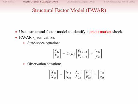
Structural Factor Model (FAVAR)
• Use a structural factor model to identify a credit market shock.• FAVAR specification:
I State-space equation:[F1t
F2t
]= Φ(L)
[F1,t−1
F2,t−1
]+
[ε1tε2t
]I Observation equation:[
X1t
X2t
]=
[Λ11 Λ21
Λ21 Λ22
] [F ′1tF ′2t
]+
[ν1t
ν2t
]

CSV Model Gilchrist, Yankov & Zakrajsek (2009) Gilchrist and Zakrajsek (2012) BMA Forecasting: FGWZ (2012)
Estimation and Identification
• Observable variables and factors can be divided into 2 groups:• Group 1: variables (X1t) and factors (F1t) related to the real,
nominal, and the financial side of the economy• Group 2: variables (X2t) and factors (F2t) pertaining to the
corporate bond market

CSV Model Gilchrist, Yankov & Zakrajsek (2009) Gilchrist and Zakrajsek (2012) BMA Forecasting: FGWZ (2012)
4-step Estimation Procedure:
• Extract F1t as the first k1 principle components of X1t
• Regress X2t on F1t and take the residuals Et• Extract F2 as the first k2 principle components of Et• Estimate matrices of factor loadings (Λ11, Λ21, Λ22) from the
measurement equation by regression (imposing the restrictionthat Λ12 = 0)

CSV Model Gilchrist, Yankov & Zakrajsek (2009) Gilchrist and Zakrajsek (2012) BMA Forecasting: FGWZ (2012)
Identifying credit market shocks:
• Impose identification on factor model.• Recursive identification scheme: F2t orthogonal to F1t
• This is equivalent to ordering F2t last in the Choleskydecomposition of Σε = E(εε′)

CSV Model Gilchrist, Yankov & Zakrajsek (2009) Gilchrist and Zakrajsek (2012) BMA Forecasting: FGWZ (2012)
Specification
• Group 1 variables (X1t):I Economic Activity (11): unemployment rate, employment
growth; industrial production; durable and nondurable goodsorders, consumer spending, etc.
I Inflation Indicators (6): CPI, core CPI, PPI, core PPI, commodityand oil prices (WTI)
I Real Interest Rates (7): funds rate, Treasury yields (6-month,1-year, . . ., 10-year)
I Financial Asset Indicators (12): excess market return, excessequity returns by EDF quintile, Fama-French factors (HML,SMB) option-implied volatilities on equity prices and short- andlong-term interest rates, foreign exchange value of the dollar
• Group 2 variables (X2t):I EDF-based portfolios of credit spreads (20)
• Baseline specification: k1 = 4, k2 = 2, p = 6.
CSV Model Gilchrist, Yankov & Zakrajsek (2009) Gilchrist and Zakrajsek (2012) BMA Forecasting: FGWZ (2012)
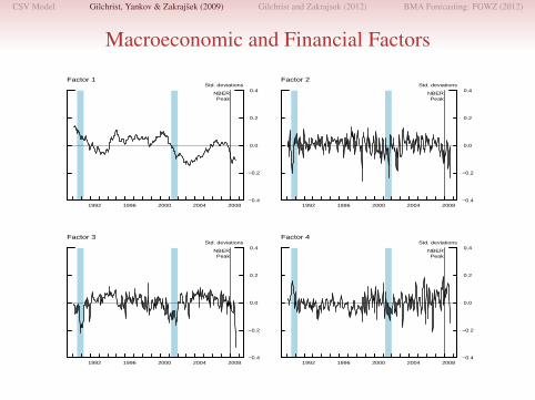
Macroeconomic and Financial Factors
1992 1996 2000 2004 2008−0.4
−0.2
0.0
0.2
0.4Std. deviations
Factor 1
NBERPeak
1992 1996 2000 2004 2008−0.4
−0.2
0.0
0.2
0.4Std. deviations
Factor 2
NBERPeak
1992 1996 2000 2004 2008−0.4
−0.2
0.0
0.2
0.4Std. deviations
Factor 3
NBERPeak
1992 1996 2000 2004 2008−0.4
−0.2
0.0
0.2
0.4Std. deviations
Factor 4
NBERPeak

CSV Model Gilchrist, Yankov & Zakrajsek (2009) Gilchrist and Zakrajsek (2012) BMA Forecasting: FGWZ (2012)
Credit Factors
1992 1996 2000 2004 2008−0.3
−0.2
−0.1
0.0
0.1
0.2
0.3Std. deviations
Factor 1
NBERPeak
1992 1996 2000 2004 2008−0.3
−0.2
−0.1
0.0
0.1
0.2
0.3Std. deviations
Factor 2
NBERPeak

CSV Model Gilchrist, Yankov & Zakrajsek (2009) Gilchrist and Zakrajsek (2012) BMA Forecasting: FGWZ (2012)
Response of Corporate Bond Spreads
0 12 24 36 48
0.0
0.1
0.2
0.3
0.4
0.5
0.6Percentage points
Months after shock
Quintile 1Quintile 2Quintile 3Quintile 4Quintile 5
Short maturity credit spreads by EDF quintile*
* Bonds with term to maturity under 3 years.
0 12 24 36 48
0.0
0.1
0.2
0.3
0.4
0.5Percentage points
Months after shock
Quintile 1Quintile 2Quintile 3Quintile 4Quintile 5
Intermediate maturity credit spreads by EDF quintile*
* Bonds with term to maturity 3−7 years.
0 12 24 36 48
0.0
0.1
0.2
0.3
0.4
0.5
0.6Percentage points
Months after shock
Quintile 1Quintile 2Quintile 3Quintile 4Quintile 5
Long maturity credit spreads by EDF quintile*
* Bonds with term to maturity 7−15 years.
0 12 24 36 48
0.0
0.1
0.2
0.3
0.4
0.5Percentage points
Months after shock
Quintile 1Quintile 2Quintile 3Quintile 4Quintile 5
Very long maturity credit spreads by EDF quintile*
* Bonds with term to maturity above 15 years.

CSV Model Gilchrist, Yankov & Zakrajsek (2009) Gilchrist and Zakrajsek (2012) BMA Forecasting: FGWZ (2012)
Response of Selected Variables
0 12 24 36 48
−2.5
−2.0
−1.5
−1.0
−0.5
0.0
0.5Percentage points
Months after shock
Industrial production
0 12 24 36 48
−2.5
−2.0
−1.5
−1.0
−0.5
0.0
0.5Percentage points
Months after shock
0 12 24 36 48
−0.4
−0.3
−0.2
−0.1
0.0
0.1Percentage points
Months after shock
Core CPI
0 12 24 36 48
−0.4
−0.3
−0.2
−0.1
0.0
0.1Percentage points
Months after shock
0 12 24 36 48
−0.30−0.25−0.20−0.15−0.10−0.05 0.00 0.05 0.10
Percentage points
Months after shock
Real federal funds rate
0 12 24 36 48
−0.30−0.25−0.20−0.15−0.10−0.05 0.00 0.05 0.10
Percentage points
Months after shock
0 12 24 36 48−0.20
−0.15
−0.10
−0.05
0.00
0.05Percentage points
Months after shock
Real 10−year Treasury yield
0 12 24 36 48−0.20
−0.15
−0.10
−0.05
0.00
0.05Percentage points
Months after shock
0 12 24 36 48
−6
−5
−4
−3
−2
−1
0
1
2Percentage points
Months after shock
Cumulative excess stock market return
0 12 24 36 48
−6
−5
−4
−3
−2
−1
0
1
2Percentage points
Months after shock
0 12 24 36 48
−0.6
−0.4
−0.2
0.0
0.2
0.4
0.6
0.8
1.0Percentage points
Months after shock
S&P 500 implied volatility (VIX)
0 12 24 36 48
−0.6
−0.4
−0.2
0.0
0.2
0.4
0.6
0.8
1.0Percentage points
Months after shock
0 12 24 36 48
−5
−4
−3
−2
−1
0
1
2Percentage points
Months after shock
Cumulative excess stock return EDF Quintile 1
0 12 24 36 48
−5
−4
−3
−2
−1
0
1
2Percentage points
Months after shock
0 12 24 36 48
−4
−2
0
2
4
6Percentage points
Months after shock
Cumulative excess stock return EDF Quintile 5
0 12 24 36 48
−4
−2
0
2
4
6Percentage points
Months after shock
CSV Model Gilchrist, Yankov & Zakrajsek (2009) Gilchrist and Zakrajsek (2012) BMA Forecasting: FGWZ (2012)
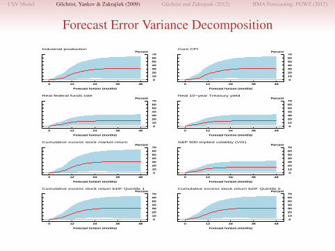
Forecast Error Variance Decomposition
0 12 24 36 48
0
10
20
30
40
50
60
70Percent
Forecast horizon (months)
Industrial production
0 12 24 36 48
0
10
20
30
40
50
60
70Percent
Forecast horizon (months)
0 12 24 36 48
0
10
20
30
40
50
60
70Percent
Forecast horizon (months)
Core CPI
0 12 24 36 48
0
10
20
30
40
50
60
70Percent
Forecast horizon (months)
0 12 24 36 48
0
10
20
30
40
50
60
70Percent
Forecast horizon (months)
Real federal funds rate
0 12 24 36 48
0
10
20
30
40
50
60
70Percent
Forecast horizon (months)
0 12 24 36 48
0
10
20
30
40
50
60
70Percent
Forecast horizon (months)
Real 10−year Treasury yield
0 12 24 36 48
0
10
20
30
40
50
60
70Percent
Forecast horizon (months)
0 12 24 36 48
0
10
20
30
40
50
60
70Percent
Forecast horizon (months)
Cumulative excess stock market return
0 12 24 36 48
0
10
20
30
40
50
60
70Percent
Forecast horizon (months)
0 12 24 36 48
0
10
20
30
40
50
60
70Percent
Forecast horizon (months)
S&P 500 implied volatility (VIX)
0 12 24 36 48
0
10
20
30
40
50
60
70Percent
Forecast horizon (months)
0 12 24 36 48
0
10
20
30
40
50
60
70Percent
Forecast horizon (months)
Cumulative excess stock return EDF Quintile 1
0 12 24 36 48
0
10
20
30
40
50
60
70Percent
Forecast horizon (months)
0 12 24 36 48
0
10
20
30
40
50
60
70Percent
Forecast horizon (months)
Cumulative excess stock return EDF Quintile 5
0 12 24 36 48
0
10
20
30
40
50
60
70Percent
Forecast horizon (months)

CSV Model Gilchrist, Yankov & Zakrajsek (2009) Gilchrist and Zakrajsek (2012) BMA Forecasting: FGWZ (2012)
Summary of Results
• Predictive content of credit spreads is concentrated inlong-maturity corporate bonds issued by medium-risk firms.
• Shocks to medium-risk, long-maturity credit spreads account fora significant fraction of the variance in economic activity at1–2 year horizon over the 1990–2008 period.

CSV Model Gilchrist, Yankov & Zakrajsek (2009) Gilchrist and Zakrajsek (2012) BMA Forecasting: FGWZ (2012)
CREDIT SPREADS AND ECONOMIC FLUCTUATIONS
• Predictive content could reflect disruption in the supply of creditstemming from:
I Worsening of the quality of borrowers’ balance sheets(Kiyotaki & Moore [1997]; Bernanke, Gertler & Gilchrist [1999]; Hall [2010])
I Deterioration in the health of financial intermediaries(Gertler & Karadi [2009]; Gertler & Kiyotaki [2009])
• Predictive content could reflect the ability of the corporate bondmarket to signal more accurately than the stock market a declinein economic fundamentals.(Philippon [2009])

CSV Model Gilchrist, Yankov & Zakrajsek (2009) Gilchrist and Zakrajsek (2012) BMA Forecasting: FGWZ (2012)
GILCHRIST AND ZAKRAJSEK (2012)
• Re-examine the evidence on the relationship between creditspreads and economic activity over the 1973–2010 period.
• Use prices of individual securities to construct a credit spreadwith a high information content for future economic activity.
• Decompose the predictive content of credit spread into:I Component capturing countercyclical movements in expected
defaultsI Component—the excess bond premium (EBP)—representing
cyclical changes in the relationship between expected default riskand credit spreads
• Decomposition motivated in part by the “credit spread puzzle.”(Elton et al. [2009]; Collin-Dufresne et al. [2001]; Driessen [2005])

CSV Model Gilchrist, Yankov & Zakrajsek (2009) Gilchrist and Zakrajsek (2012) BMA Forecasting: FGWZ (2012)
MAIN FINDINGS
• Predictive content of credit spreads for economic activity isalmost entirely due to movements in the EBP.
• Unanticipated increases in the EBP:I Lead to significant and protracted declines in economic activity
and the stock marketI Account for a substantial fraction of the variation in real activity
and stock market at business cycle frequencies

CSV Model Gilchrist, Yankov & Zakrajsek (2009) Gilchrist and Zakrajsek (2012) BMA Forecasting: FGWZ (2012)
BOND-LEVEL DATA
• CRSP/Compustat panel of U.S. nonfinancial firms matched withprices of outstanding corporate bonds traded in the secondarymarket.
• Lehman/Warga & Merrill Lynch issue-level data:I Sample period: Jan1973–Jun2010 (month-end)I 1,116 U.S. nonfinancial issuersI 5,942 senior unsecured (fixed-coupon) bond issuesI 338,615 observationsI Information: price, issue date, maturity, coupon, issue size, etc.

CSV Model Gilchrist, Yankov & Zakrajsek (2009) Gilchrist and Zakrajsek (2012) BMA Forecasting: FGWZ (2012)
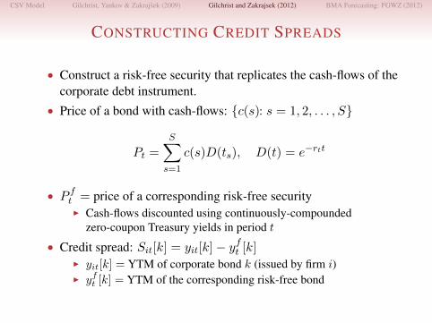
CONSTRUCTING CREDIT SPREADS
• Construct a risk-free security that replicates the cash-flows of thecorporate debt instrument.
• Price of a bond with cash-flows: {c(s): s = 1, 2, . . . , S}
Pt =
S∑s=1
c(s)D(ts), D(t) = e−rtt
• P ft = price of a corresponding risk-free securityI Cash-flows discounted using continuously-compounded
zero-coupon Treasury yields in period t
• Credit spread: Sit[k] = yit[k]− yft [k]I yit[k] = YTM of corporate bond k (issued by firm i)I yft [k] = YTM of the corresponding risk-free bond

CSV Model Gilchrist, Yankov & Zakrajsek (2009) Gilchrist and Zakrajsek (2012) BMA Forecasting: FGWZ (2012)
CONSTRUCTING CREDIT SPREADS
• Construct a risk-free security that replicates the cash-flows of thecorporate debt instrument.
• Price of a bond with cash-flows: {c(s): s = 1, 2, . . . , S}
Pt =
S∑s=1
c(s)D(ts), D(t) = e−rtt
• P ft = price of a corresponding risk-free securityI Cash-flows discounted using continuously-compounded
zero-coupon Treasury yields in period t
• Credit spread: Sit[k] = yit[k]− yft [k]I yit[k] = YTM of corporate bond k (issued by firm i)I yft [k] = YTM of the corresponding risk-free bond

CSV Model Gilchrist, Yankov & Zakrajsek (2009) Gilchrist and Zakrajsek (2012) BMA Forecasting: FGWZ (2012)
SUMMARY STATISTICS OF BOND CHARACTERISTICS(Jan1973–Jun2010)
Variable Mean SD Min P50 Max
No. of bonds per firm/month 2.89 3.54 1.00 2.00 74.0Mkt. value of issue ($mil.) 317.9 319.7 1.22 236.1 5,628Maturity at issue (years) 13.0 9.3 1.0 10.0 50.0Term to maturity (years) 11.3 8.5 1.0 8.2 30.0Duration (years) 6.48 3.19 0.91 6.08 15.8Credit rating (S&P) - - D BBB1 AAACoupon rate (pct.) 7.32 2.00 1.70 7.00 17.5Nominal effective yield (pct.) 7.73 3.23 0.60 7.19 44.3Credit spread (bps.) 203 281 5 116 3,499
• GZ spread: cross-sectional average of credit spreads in period t
SGZt =
1
Nt
∑i
∑k
Sit[k]
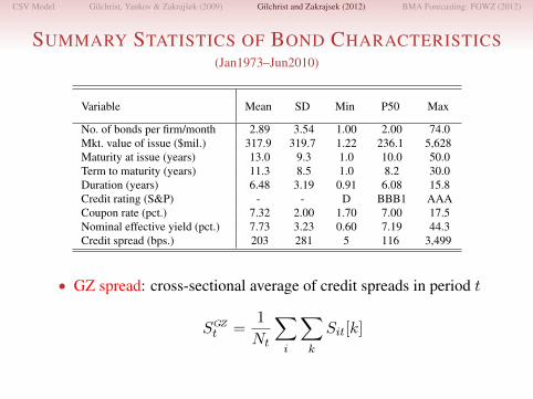

CSV Model Gilchrist, Yankov & Zakrajsek (2009) Gilchrist and Zakrajsek (2012) BMA Forecasting: FGWZ (2012)
SELECTED CORPORATE CREDIT SPREADS(Jan1973–Jun2010)
1973 1976 1979 1982 1985 1988 1991 1994 1997 2000 2003 2006 2009-1
0
1
2
3
4
5
6
7
8Percentage points
GZ spreadBaa-Aaa spreadCP-Bill spread
Monthly

CSV Model Gilchrist, Yankov & Zakrajsek (2009) Gilchrist and Zakrajsek (2012) BMA Forecasting: FGWZ (2012)
PREDICTIVE CONTENT OF CREDIT SPREADS
• Forecasting specification (h-periods ahead):
∇hYt+h = α+
p∑i=0
βi∇Yt−i + γ1TSt + γ2RFFt + γ3CSt + εt+h
I ∇hYt+h ≡ ch ln
(Yt+hYt
), where (c = 400/1, 200)
I Yt = measure of economic activityI TSt = term spread (Treas3mo − Treas10yr)I RFFt = real federal funds rate (nominal FFR − core PCE infl.)I CSt = credit spread (paper-bill, Baa-Aaa, GZ)
• Estimated by OLS w/ Hodrick (1992) SEs.

CSV Model Gilchrist, Yankov & Zakrajsek (2009) Gilchrist and Zakrajsek (2012) BMA Forecasting: FGWZ (2012)
ECONOMIC INDICATOR: PAYROLL EMPLOYMENT(Sample period: Jan1973–Jun2010)
Financial Indicator Forecast Horizon: 3 months Forecast Horizon: 12 months
Term spread -0.082 -0.087 -0.086 -0.099 -0.238 -0.239 -0.219 -0.267[1.94] [2.05] [2.06] [2.39] [4.82] [4.79] [4.71] [5.54]
Real FFR -0.083 -0.011 -0.077 -0.132 -0.125 -0.111 -0.157 -0.208[1.82] [0.18] [1.67] [2.84] [2.38] [1.75] [3.15] [4.09]
CP-bill spread - -0.108 - - - -0.022 - -[2.40] [0.64]
Baa–Aaa spread - - -0.020 - - - 0.111 -[0.52] [2.31]
GZ spread - - - -0.272 - - - -0.457[6.61] [12.4]
Adj. R2 0.661 0.667 0.660 0.705 0.448 0.447 0.456 0.577
NOTE: Parameter estimates are standardized; absolute t-statistics in brackets.

CSV Model Gilchrist, Yankov & Zakrajsek (2009) Gilchrist and Zakrajsek (2012) BMA Forecasting: FGWZ (2012)
ECONOMIC INDICATOR: REAL GDP(Sample period: 1973:Q1–2010:Q2)
Financial Indicator Forecast Horizon: 1 quarter Forecast Horizon: 4 quarters
Term spread -0.143 -0.175 -0.158 -0.200 -0.382 -0.385 -0.371 -0.423[1.38] [1.63] [1.36] [1.95] [2.86] [2.85] [2.62] [3.39]
Real FFR -0.103 0.110 -0.093 -0.162 -0.066 -0.032 -0.072 -0.155[0.97] [0.76] [0.87] [1.57] [0.50] [0.19] [0.54] [1.16]
CP-bill spread - -0.254 - - - -0.048 - -[2.33] [0.42]
Baa–Aaa spread - - -0.059 - - - 0.052 -[0.51] [0.44]
GZ spread - - - -0.327 - - - -0.348[3.98] [3.66]
Adj. R2 0.176 0.191 0.173 0.235 0.239 0.235 0.236 0.325
NOTE: Parameter estimates are standardized; absolute t-statistics in brackets.

CSV Model Gilchrist, Yankov & Zakrajsek (2009) Gilchrist and Zakrajsek (2012) BMA Forecasting: FGWZ (2012)
FRAMEWORK
• Empirical bond-pricing model:
lnSit[k] = β0 + β1DFTit + β2Zit[k] + εit[k]
I Sit[k] = credit spread on bond k (issued by firm i)I DFTit = measure of expected default risk for firm iI Zit[k] = bond-specific control variablesI εit[k] = “pricing error”
• Estimated by OLS w/ two-way clustered SEs.

CSV Model Gilchrist, Yankov & Zakrajsek (2009) Gilchrist and Zakrajsek (2012) BMA Forecasting: FGWZ (2012)
CREDIT SPREAD DECOMPOSITION
• Predicted level of the spread for bond k:
Sit[k] = θSit[k]
I Sit[k] = exp(β0 + β1DFTit + β′3Zit)I θ obtained from pooled regression: Sit[k] = θSit[k] + νit[k]
• Predicted GZ spread:
SGZt =
1
Nt
∑i
∑k
Sit[k]
• The excess bond premium:
EBPt = SGZt − SGZ
t

CSV Model Gilchrist, Yankov & Zakrajsek (2009) Gilchrist and Zakrajsek (2012) BMA Forecasting: FGWZ (2012)
DEFAULT RISK
• Merton distance-to-default (DD) model:I Value of the firm (V ) follows a geometric Brownian motion
dV = µV V dt+ σV V dW
I Firm has just issued a discount bond (D) maturing in T periods
• Distance-to-default (1-year horizon):
DD =ln(V/D) + (µV − 0.5σ2V )
σV
I V , µV , σV estimated using data on E, D, µE , σE(Bharath & Shumway [2008])
• Sample: U.S. nonfinancial corporate sector (≈ 11, 000 firms)
CSV Model Gilchrist, Yankov & Zakrajsek (2009) Gilchrist and Zakrajsek (2012) BMA Forecasting: FGWZ (2012)
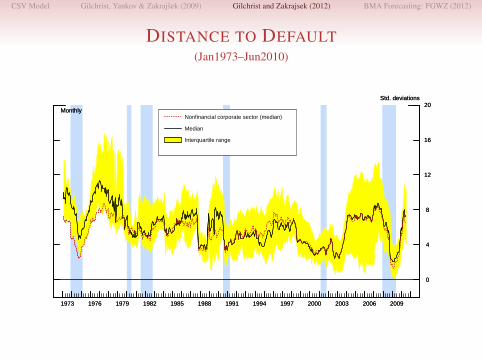
DISTANCE TO DEFAULT(Jan1973–Jun2010)
1973 1976 1979 1982 1985 1988 1991 1994 1997 2000 2003 2006 2009
0
4
8
12
16
20Std. deviations
Monthly
1973 1976 1979 1982 1985 1988 1991 1994 1997 2000 2003 2006 2009
0
4
8
12
16
20Std. deviations
Monthly
Interquartile range
Nonfinancial corporate sector (median)
Median

CSV Model Gilchrist, Yankov & Zakrajsek (2009) Gilchrist and Zakrajsek (2012) BMA Forecasting: FGWZ (2012)
DISTANCE TO DEFAULT AND ACTUAL DEFAULT RATE(Jan1981–Sep2010)
1
2
3
4
5
6
7
8
9
1981 1983 1985 1987 1989 1991 1993 1995 1997 1999 2001 2003 2005 2007 20090
1
2
3
4
5
6
7
8Standard deviations Percent of outstanding
Weighted median distance-to-default at t-12 (left scale)Actual 12-month default rate at t (right scale)
Monthly
CSV Model Gilchrist, Yankov & Zakrajsek (2009) Gilchrist and Zakrajsek (2012) BMA Forecasting: FGWZ (2012)
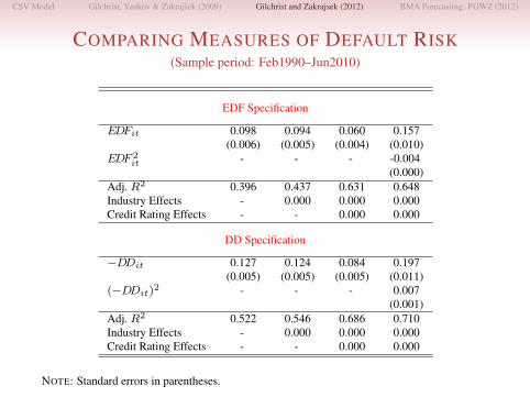
COMPARING MEASURES OF DEFAULT RISK(Sample period: Feb1990–Jun2010)
EDF Specification
EDFit 0.098 0.094 0.060 0.157(0.006) (0.005) (0.004) (0.010)
EDF 2it - - - -0.004
(0.000)Adj. R2 0.396 0.437 0.631 0.648Industry Effects - 0.000 0.000 0.000Credit Rating Effects - - 0.000 0.000
DD Specification
−DDit 0.127 0.124 0.084 0.197(0.005) (0.005) (0.005) (0.011)
(−DDit)2 - - - 0.007
(0.001)Adj. R2 0.522 0.546 0.686 0.710Industry Effects - 0.000 0.000 0.000Credit Rating Effects - - 0.000 0.000
NOTE: Standard errors in parentheses.

CSV Model Gilchrist, Yankov & Zakrajsek (2009) Gilchrist and Zakrajsek (2012) BMA Forecasting: FGWZ (2012)
CALLABLE CORPORATE DEBT(Jan1973–Jun2010)
1973 1976 1979 1982 1985 1988 1991 1994 1997 2000 2003 2006 2009 0
20
40
60
80
100
Percent
Proportion of total bondsProportion of total par value
Monthly

CSV Model Gilchrist, Yankov & Zakrajsek (2009) Gilchrist and Zakrajsek (2012) BMA Forecasting: FGWZ (2012)
OPTION-ADJUSTED EXCESS BOND PREMIUM
• Movements in risk-free rates—by changing the value ofembedded call options—have an independent effect on prices ofcallable bonds.(Duffee [1998])
• Prices of callable bonds are more sensitive to uncertaintyregarding the future course of interest rates.
• Option-adjusted EBP:I Include call-option indicator in the bond-pricing regressionI Spreads on callable bonds are allowed to depend on the level,
slope, and curvature factors, as well as on interest rate volatility
CSV Model Gilchrist, Yankov & Zakrajsek (2009) Gilchrist and Zakrajsek (2012) BMA Forecasting: FGWZ (2012)
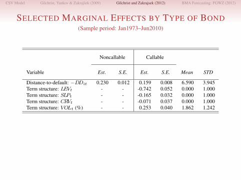
SELECTED MARGINAL EFFECTS BY TYPE OF BOND(Sample period: Jan1973–Jun2010)
Noncallable Callable
Variable Est. S.E. Est. S.E. Mean STD
Distance-to-default: −DDit 0.230 0.012 0.159 0.008 6.590 3.945Term structure: LEVt - - -0.742 0.052 0.000 1.000Term structure: SLPt - - -0.165 0.032 0.000 1.000Term structure: CRVt - - -0.071 0.037 0.000 1.000Term structure: VOLt (%) - - 0.253 0.040 1.862 1.242

CSV Model Gilchrist, Yankov & Zakrajsek (2009) Gilchrist and Zakrajsek (2012) BMA Forecasting: FGWZ (2012)
ACTUAL AND PREDICTED CREDIT SPREADS(Jan1973–Jun2010)
1973 1976 1979 1982 1985 1988 1991 1994 1997 2000 2003 2006 20090
2
4
6
8Percentage points
Actual GZ spreadPredicted GZ spread w/ option adjustmentsPredicted GZ spread w/o option adjustments
Monthly

CSV Model Gilchrist, Yankov & Zakrajsek (2009) Gilchrist and Zakrajsek (2012) BMA Forecasting: FGWZ (2012)
OPTION-ADJUSTED EXCESS BOND PREMIUM(Jan1973–Jun2010)
1973 1976 1979 1982 1985 1988 1991 1994 1997 2000 2003 2006 2009-2
-1
0
1
2
3Percentage points
Monthly
CSV Model Gilchrist, Yankov & Zakrajsek (2009) Gilchrist and Zakrajsek (2012) BMA Forecasting: FGWZ (2012)
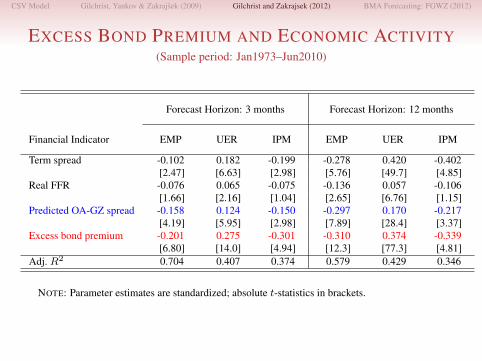
EXCESS BOND PREMIUM AND ECONOMIC ACTIVITY(Sample period: Jan1973–Jun2010)
Forecast Horizon: 3 months Forecast Horizon: 12 months
Financial Indicator EMP UER IPM EMP UER IPM
Term spread -0.102 0.182 -0.199 -0.278 0.420 -0.402[2.47] [6.63] [2.98] [5.76] [49.7] [4.85]
Real FFR -0.076 0.065 -0.075 -0.136 0.057 -0.106[1.66] [2.16] [1.04] [2.65] [6.76] [1.15]
Predicted OA-GZ spread -0.158 0.124 -0.150 -0.297 0.170 -0.217[4.19] [5.95] [2.98] [7.89] [28.4] [3.37]
Excess bond premium -0.201 0.275 -0.301 -0.310 0.374 -0.339[6.80] [14.0] [4.94] [12.3] [77.3] [4.81]
Adj. R2 0.704 0.407 0.374 0.579 0.429 0.346
NOTE: Parameter estimates are standardized; absolute t-statistics in brackets.

CSV Model Gilchrist, Yankov & Zakrajsek (2009) Gilchrist and Zakrajsek (2012) BMA Forecasting: FGWZ (2012)
EXCESS BOND PREMIUM AND REAL GDP(Sample period: 1973:Q1–2010:Q2)
Financial Indicator Forecast Horizon: 1 quarter Forecast Horizon: 4 quarters
Term spread -0.213 -0.231[2.07] [3.35]
Real FFR -0.084 -0.090[0.79] [0.66]
Predicted OA-GZ spread -0.123 -0.166[1.69] [1.68]
Excess bond premium -0.290 -0.238[3.91] [2.96]
Adj. R2 0.239 0.307
NOTE: Parameter estimates are standardized; absolute t-statistics in brackets.

CSV Model Gilchrist, Yankov & Zakrajsek (2009) Gilchrist and Zakrajsek (2012) BMA Forecasting: FGWZ (2012)
EXCESS BOND PREMIUM AND AD-COMPONENTS(Sample period: 1973:Q1–2010:Q2)
Forecast Horizon: 4 quarters
Financial Indicator C-NDS C-D I-RES I-ES I-HT I-NRS INV
Term spread -0.395 -0.511 -0.529 -0.378 -0.085 0.329 -0.136[3.79] [2.64] [5.40] [3.41] [0.76] [2.78] [1.65]
Real FFR 0.128 0.110 0.037 -0.137 -0.158 -0.175 -0.059[1.35] [0.65] [0.33] [1.42] [1.16] [1.49] [0.68]
Predicted OA-GZ spread -0.144 0.088 -0.083 -0.147 -0.331 -0.141 -0.225[1.67] [0.68] [1.14] [1.60] [3.51] [1.64] [3.40]
Excess bond premium -0.152 -0.075 0.042 -0.465 -0.301 -0.553 -0.603[2.15] [0.56] [0.60] [4.22] [3.24] [5.35] [8.53]
Adj. R2 0.366 0.193 0.376 0.418 0.386 0.533 0.554
NOTE: Parameter estimates are standardized; absolute t-statistics in brackets.

CSV Model Gilchrist, Yankov & Zakrajsek (2009) Gilchrist and Zakrajsek (2012) BMA Forecasting: FGWZ (2012)
ROBUSTNESS CHECK: 1985–2010 PERIOD
• Apparent decline in macroeconomic volatility since themid-1980s:
I Changes in the conduct of monetary policyI Changes in government policy (e.g., demise of Regulation Q)I Rapid growth of securities markets
• Changes in the structure of the corporate bond market:I Re-emergence of the market for speculative-grade debtI Decline in information costs associated with credit-risk analysisI Changes in investors’ risk perceptions

CSV Model Gilchrist, Yankov & Zakrajsek (2009) Gilchrist and Zakrajsek (2012) BMA Forecasting: FGWZ (2012)
EXCESS BOND PREMIUM AND REAL GDP(Sample period: 1985:Q1–2010:Q2)
Financial Indicator Forecast Horizon: 1 quarter Forecast Horizon: 4 quarters
Term spread -0.308 -0.449[2.32] [3.35]
Real FFR 0.384 0.360[2.08] [2.17]
Predicted OA-GZ spread 0.101 0.080[0.86] [0.58]
Excess bond premium -0.423 -0.436[3.25] [3.86]
Adj. R2 0.357 0.275
NOTE: Parameter estimates are standardized; absolute t-statistics in brackets.
CSV Model Gilchrist, Yankov & Zakrajsek (2009) Gilchrist and Zakrajsek (2012) BMA Forecasting: FGWZ (2012)
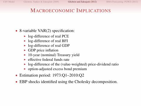
MACROECONOMIC IMPLICATIONS
• 8-variable VAR(2) specification:I log-difference of real PCEI log-difference of real BFII log-difference of real GDPI GDP price inflationI 10-year (nominal) Treasury yieldI effective federal funds rateI log-difference of the (value-weighted) price-dividend ratioI option-adjusted excess bond premium
• Estimation period: 1973:Q1–2010:Q2• EBP shocks identified using the Cholesky decomposition.

CSV Model Gilchrist, Yankov & Zakrajsek (2009) Gilchrist and Zakrajsek (2012) BMA Forecasting: FGWZ (2012)
ADVERSE EBP SHOCKMacroeconomic Variables
0 2 4 6 8 10 12 14 16 18 20-0.8
-0.6
-0.4
-0.2
0.0
0.2
0.4Percentage points
Quarters after shock
0 2 4 6 8 10 12 14 16 18 20-0.8
-0.6
-0.4
-0.2
0.0
0.2
0.4Percentage points
Quarters after shock
Consumption
0 2 4 6 8 10 12 14 16 18 20-5
-4
-3
-2
-1
0
1Percentage points
Quarters after shock
0 2 4 6 8 10 12 14 16 18 20-5
-4
-3
-2
-1
0
1Percentage points
Quarters after shock
Investment
0 2 4 6 8 10 12 14 16 18 20-1.0
-0.8
-0.6
-0.4
-0.2
0.0
0.2
0.4Percentage points
Quarters after shock
0 2 4 6 8 10 12 14 16 18 20-1.0
-0.8
-0.6
-0.4
-0.2
0.0
0.2
0.4Percentage points
Quarters after shock
Output
0 2 4 6 8 10 12 14 16 18 20-2.0
-1.5
-1.0
-0.5
0.0
0.5Percentage points
Quarters after shock
0 2 4 6 8 10 12 14 16 18 20-2.0
-1.5
-1.0
-0.5
0.0
0.5Percentage points
Quarters after shock
Prices
NOTE: Shaded bands denote 95-percent confidence intervals.

CSV Model Gilchrist, Yankov & Zakrajsek (2009) Gilchrist and Zakrajsek (2012) BMA Forecasting: FGWZ (2012)
ADVERSE EBP SHOCKFinancial Variables
0 2 4 6 8 10 12 14 16 18 20-8
-6
-4
-2
0
2Percentage points
Quarters after shock
0 2 4 6 8 10 12 14 16 18 20-8
-6
-4
-2
0
2Percentage points
Quarters after shock
Price-dividend ratio
0 2 4 6 8 10 12 14 16 18 20-0.5
-0.4
-0.3
-0.2
-0.1
0.0
0.1Percentage points
Quarters after shock
0 2 4 6 8 10 12 14 16 18 20-0.5
-0.4
-0.3
-0.2
-0.1
0.0
0.1Percentage points
Quarters after shock
10-year Treasury yield
0 2 4 6 8 10 12 14 16 18 20-1.0
-0.8
-0.6
-0.4
-0.2
0.0
0.2Percentage points
Quarters after shock
0 2 4 6 8 10 12 14 16 18 20-1.0
-0.8
-0.6
-0.4
-0.2
0.0
0.2Percentage points
Quarters after shock
Federal funds rate
0 2 4 6 8 10 12 14 16 18 20-0.10
-0.05
0.00
0.05
0.10
0.15
0.20
0.25
0.30Percentage points
Quarters after shock
0 2 4 6 8 10 12 14 16 18 20-0.10
-0.05
0.00
0.05
0.10
0.15
0.20
0.25
0.30Percentage points
Quarters after shock
Excess bond premium
NOTE: Shaded bands denote 95-percent confidence intervals.

CSV Model Gilchrist, Yankov & Zakrajsek (2009) Gilchrist and Zakrajsek (2012) BMA Forecasting: FGWZ (2012)
FORECAST ERROR VARIANCE DECOMPOSITIONMacroeconomic Variables
0 2 4 6 8 10 12 14 16 18 20
0
10
20
30
40
50Percent
Forecast horizon (quarters)
0 2 4 6 8 10 12 14 16 18 20
0
10
20
30
40
50Percent
Forecast horizon (quarters)
Consumption
0 2 4 6 8 10 12 14 16 18 20
0
10
20
30
40
50Percent
Forecast horizon (quarters)
0 2 4 6 8 10 12 14 16 18 20
0
10
20
30
40
50Percent
Forecast horizon (quarters)
Investment
0 2 4 6 8 10 12 14 16 18 20
0
10
20
30
40
50Percent
Forecast horizon (quarters)
0 2 4 6 8 10 12 14 16 18 20
0
10
20
30
40
50Percent
Forecast horizon (quarters)
Output
0 2 4 6 8 10 12 14 16 18 20
0
10
20
30
40
50Percent
Forecast horizon (quarters)
0 2 4 6 8 10 12 14 16 18 20
0
10
20
30
40
50Percent
Forecast horizon (quarters)
Prices
NOTE: Shaded bands denote 95-percent confidence intervals.

CSV Model Gilchrist, Yankov & Zakrajsek (2009) Gilchrist and Zakrajsek (2012) BMA Forecasting: FGWZ (2012)
FORECAST ERROR VARIANCE DECOMPOSITIONFinancial Variables
0 2 4 6 8 10 12 14 16 18 20
0
10
20
30
40
50Percent
Forecast horizon (quarters)
0 2 4 6 8 10 12 14 16 18 20
0
10
20
30
40
50Percent
Forecast horizon (quarters)
Price-dividend ratio
0 2 4 6 8 10 12 14 16 18 20
0
10
20
30
40
50Percent
Forecast horizon (quarters)
0 2 4 6 8 10 12 14 16 18 20
0
10
20
30
40
50Percent
Forecast horizon (quarters)
10-year Treasury yield
0 2 4 6 8 10 12 14 16 18 20
0
10
20
30
40
50Percent
Forecast horizon (quarters)
0 2 4 6 8 10 12 14 16 18 20
0
10
20
30
40
50Percent
Forecast horizon (quarters)
Federal funds rate
0 2 4 6 8 10 12 14 16 18 20
0
20
40
60
80
100Percent
Forecast horizon (quarters)
0 2 4 6 8 10 12 14 16 18 20
0
20
40
60
80
100Percent
Forecast horizon (quarters)
Excess bond premium
NOTE: Shaded bands denote 95-percent confidence intervals.

CSV Model Gilchrist, Yankov & Zakrajsek (2009) Gilchrist and Zakrajsek (2012) BMA Forecasting: FGWZ (2012)
INTERPRETATION
• The EBP provides a timely gauge of credit-supply conditions.• Increase in the EBP leads to an economic downturn vis-a-vis the
financial accelerator mechanism.• Financial shocks may also cause variation in the risk attitudes of
the marginal investor pricing corporate bonds:I Corporate bond market is dominated by large institutional
investorsI These financial intermediaries face capital requirementsI A shock to their financial capital makes them act in a more
risk-averse mannerI Shift in their risk attitudes leads to an increase in the EBP
(He & Krishnamurthy [2010]; Adrian, Moench & Shin [2010])

CSV Model Gilchrist, Yankov & Zakrajsek (2009) Gilchrist and Zakrajsek (2012) BMA Forecasting: FGWZ (2012)
EBP & CHANGES IN BANK LENDING STANDARDS(Jan1973–Sep2010)
-1.0
-0.5
0.0
0.5
1.0
1.5
2.0
1973 1976 1979 1982 1985 1988 1991 1994 1997 2000 2003 2006 2009-50
-25
0
25
50
75
100Percentage points Net percent
Excess bond premium (left scale)Change in C&I lending standards (right scale)
Quarterly

CSV Model Gilchrist, Yankov & Zakrajsek (2009) Gilchrist and Zakrajsek (2012) BMA Forecasting: FGWZ (2012)
EBP & FINANCIAL SECTOR PROFITABILITY(Jan1973–Sep2010)
-6
-4
-2
0
2
4
6
1985 1987 1989 1991 1993 1995 1997 1999 2001 2003 2005 2007 2009-3
-2
-1
0
1
2
3Percentage points Percent
Financial bond premium (left scale)ROA (right scale)
MonthlyLehman Brother’s
bankruptcy
•••••
••••
•
•
••••
•••
••••••
••••••••
••••••
••••••••••••
••••••••
•••••••••••••••
••••••••
••••••
•••
•••
•
•
•
•••••
•••

CSV Model Gilchrist, Yankov & Zakrajsek (2009) Gilchrist and Zakrajsek (2012) BMA Forecasting: FGWZ (2012)
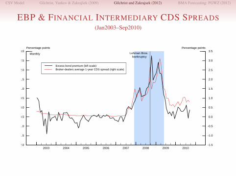
EVIDENCE FROM PRIMARY DEALERS
• Primary Dealers (PDs): major banks and broker-dealers thattrade in U.S. Government securities with the FRBNY:
I By buying/selling securities for a fee and holding an inventory ofsecurities PDs play a key role in financial markets
I PDs are often highly leveraged and engage in active pro-cyclicalmanagement of leverage
• Collected monthly data on CDS spreads and equity valuations.
CSV Model Gilchrist, Yankov & Zakrajsek (2009) Gilchrist and Zakrajsek (2012) BMA Forecasting: FGWZ (2012)
EBP & FINANCIAL INTERMEDIARY CDS SPREADS(Jan2003–Sep2010)
-2.0
-1.5
-1.0
-0.5
0.0
0.5
1.0
1.5
2.0
2.5
3.0
2003 2004 2005 2006 2007 2008 2009 2010-1.5
-1.0
-0.5
0.0
0.5
1.0
1.5
2.0
2.5
3.0
3.5Percentage points Percentage points
Excess bond premium (left scale)Broker-dealers average 1-year CDS spread (right scale)
Monthly Lehman Bros.bankruptcy

CSV Model Gilchrist, Yankov & Zakrajsek (2009) Gilchrist and Zakrajsek (2012) BMA Forecasting: FGWZ (2012)
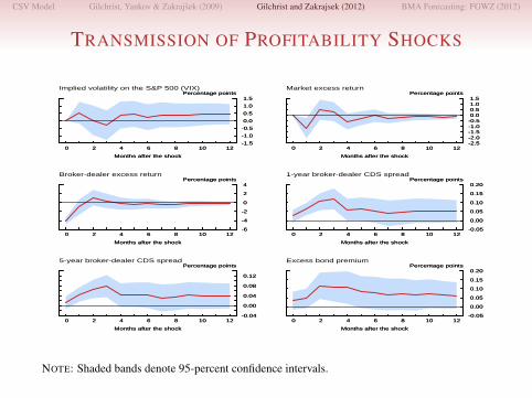
SHOCKS TO THE PROFITABILITY OF FIS
• 6-variable VAR(2) specification:I option-implied volatility on the S&P 500 (VIX)I excess (value-weighted) market returnI excess (value-weighted) portfolio return of broker-dealersI average 1-year broker-dealer CDS spreadI average 5-year broker-dealer CDS spreadI option-adjusted excess bond premiumI dummy for Sep2010 (Lehman Bros. bankruptcy)
• Estimation period: Jan2003–Sep2010• Shocks to the profitability of FIs identified using the Cholesky
decomposition.
CSV Model Gilchrist, Yankov & Zakrajsek (2009) Gilchrist and Zakrajsek (2012) BMA Forecasting: FGWZ (2012)
TRANSMISSION OF PROFITABILITY SHOCKS
0 2 4 6 8 10 12-1.5
-1.0
-0.5
0.0
0.5
1.0
1.5Percentage points
Months after the shock
0 2 4 6 8 10 12-1.5
-1.0
-0.5
0.0
0.5
1.0
1.5Percentage points
Months after the shock
Implied volatility on the S&P 500 (VIX)
0 2 4 6 8 10 12-2.5-2.0-1.5-1.0-0.5 0.0 0.5 1.0 1.5
Percentage points
Months after the shock
0 2 4 6 8 10 12-2.5-2.0-1.5-1.0-0.5 0.0 0.5 1.0 1.5
Percentage points
Months after the shock
Market excess return
0 2 4 6 8 10 12-6
-4
-2
0
2
4Percentage points
Months after the shock
0 2 4 6 8 10 12-6
-4
-2
0
2
4Percentage points
Months after the shock
Broker-dealer excess return
0 2 4 6 8 10 12-0.05
0.00
0.05
0.10
0.15
0.20Percentage points
Months after the shock
0 2 4 6 8 10 12-0.05
0.00
0.05
0.10
0.15
0.20Percentage points
Months after the shock
1-year broker-dealer CDS spread
0 2 4 6 8 10 12-0.04
0.00
0.04
0.08
0.12
Percentage points
Months after the shock
0 2 4 6 8 10 12-0.04
0.00
0.04
0.08
0.12
Percentage points
Months after the shock
5-year broker-dealer CDS spread
0 2 4 6 8 10 12-0.05
0.00
0.05
0.10
0.15
0.20Percentage points
Months after the shock
0 2 4 6 8 10 12-0.05
0.00
0.05
0.10
0.15
0.20Percentage points
Months after the shock
Excess bond premium
NOTE: Shaded bands denote 95-percent confidence intervals.

CSV Model Gilchrist, Yankov & Zakrajsek (2009) Gilchrist and Zakrajsek (2012) BMA Forecasting: FGWZ (2012)
CONCLUDING REMARKS
• Information content of credit spreads reflects:I Downside risk not well captured by other asset pricesI “Risk-aversion” of financial intermediaries
• Increases in spreads signal disruptions in credit markets that haveimportant consequences for macroeconomic outcomes.
• Integrating asset pricing with macroeconomic models used inpolicy analysis is a necessary step to understanding theinteraction between the financial sector and the real economy.

CSV Model Gilchrist, Yankov & Zakrajsek (2009) Gilchrist and Zakrajsek (2012) BMA Forecasting: FGWZ (2012)
FGWZ(2012): MOTIVATION
• Forecasting economic activity in real time is hard.• Amazingly little predictability beyond the current quarter:
(Sims [2005]; Tulip [2005]; Faust & Wright [2009]; Edge & Gurkaynak [2011])I Greenbook four-quarter-ahead forecast of real GDP growth is no
better that the unconditional mean.
• Estimated medium-scale DSGE models and complex statisticalmodels cannot beat forecasts of output growth and inflationbased on univariate autoregressions.

CSV Model Gilchrist, Yankov & Zakrajsek (2009) Gilchrist and Zakrajsek (2012) BMA Forecasting: FGWZ (2012)
FGWZ (2012): METHODOLOGY
• Provides an evaluation of the marginal information of creditspreads in real-time economic forecasting.
• Utilizes portfolio credit spreads based on an extensivemicro-level data set of secondary market bond prices.(Gilchrist, Yankov & Zakrajsek [2009]; Gilchrist & Zakrajsek [2011])
• Employs Bayesian Model Averaging (BMA) to forecastreal-time measures of economic activity using portfolio creditspreads and many other asset market indicators:
I BMA framework addresses model search and selection issues.

CSV Model Gilchrist, Yankov & Zakrajsek (2009) Gilchrist and Zakrajsek (2012) BMA Forecasting: FGWZ (2012)
MEASURING CREDIT SPREADS & DEFAULT RISK
• Construct a risk-free security replicating the cash-flows of thecorporate debt instrument:
I Cash-flows discounted using continuously-compoundedzero-coupon Treasury yields in period t.
• Measure default risk using the “distance-to-default:”(Merton [1974])
DD =ln(V/D) + (µV − 0.5σ2V )
σV
I V , µV , σV estimated using data on E, D, µE , σE .(Bharath & Shumway [2008])

CSV Model Gilchrist, Yankov & Zakrajsek (2009) Gilchrist and Zakrajsek (2012) BMA Forecasting: FGWZ (2012)
CALL OPTION ADJUSTMENT
• More than one-half of bonds in our sample are callable, onaverage.
• Movements in risk-free rates—by changing the value ofembedded call options—have an independent effect on prices ofcallable bonds.(Duffee [1998])
• Use an empirical credit-spread model to construct“option-adjusted” spreads.(Gilchrist & Zakrajsek [2011])

CSV Model Gilchrist, Yankov & Zakrajsek (2009) Gilchrist and Zakrajsek (2012) BMA Forecasting: FGWZ (2012)
AVERAGE CREDIT SPREADS(Jan1986–Jun2010)
1986 1988 1990 1992 1994 1996 1998 2000 2002 2004 2006 2008 2010 0
100
200
300
400
500
600
700Basis points
Option-adjusted credit spreadRaw credit spread
Monthly
Nonfinancial firms
1986 1988 1990 1992 1994 1996 1998 2000 2002 2004 2006 2008 2010 0
100
200
300
400
500
600
700Basis points
Option-adjusted credit spreadRaw credit spread
Monthly
Financial firms

CSV Model Gilchrist, Yankov & Zakrajsek (2009) Gilchrist and Zakrajsek (2012) BMA Forecasting: FGWZ (2012)
BOND, STOCK, AND DD PORTFOLIOS
• Procedure:I Sort bond issuers into categories based on the cross-sectional
distribution of DDs in month t− 1.I Within each DD-category, sort bonds into maturity categories.I For each month t calculate:
• Average credit spread within each DD/maturity category.• Average excess stock return within each DD category.• Average DD within each DD quartile.
• Use the same procedure to construct stock and DD portfolios forall U.S. nonfinancial and financial corporations.

CSV Model Gilchrist, Yankov & Zakrajsek (2009) Gilchrist and Zakrajsek (2012) BMA Forecasting: FGWZ (2012)
THE BMA SETUP
• n possible (linear) forecasting models:
yt+h = α+ βixit +
p∑j=1
γjyt−j + εt+h, i = 1, . . . , n
• Priors:I All models are equally likely: P (Mi) = 1/n.I Priors for α, γ1, . . . γp, σ
2: proportional to 1/σ.I g-prior for βi: N(0, φσ2(X ′iXi)
−1).

CSV Model Gilchrist, Yankov & Zakrajsek (2009) Gilchrist and Zakrajsek (2012) BMA Forecasting: FGWZ (2012)
THE BMA SETUP (CONT.)• Bayesian h-period-ahead forecast for model Mi:
yiT+h|T = α+ βixit +
p∑j=1
γjyt−j
I α, β, γ1, . . . , γp = OLS estimatesI βi =
(φφ+1
)βi = posterior mean of βi
• Posterior probabilities (given the observed data D):I Posterior probability that the Mi model is “true:”
P (Mi|D) ∝ P (D|Mi)P (Mi)
I Marginal likelihood of the Mi model:
P (D|Mi) ∝[
1
1 + φ
]− 12
×[
1
1 + φSSRi +
φ
1 + φSSEi
]− (T−p)2

CSV Model Gilchrist, Yankov & Zakrajsek (2009) Gilchrist and Zakrajsek (2012) BMA Forecasting: FGWZ (2012)
THE BMA FORECAST
• BMA forecast:
yT+h|T =
n∑i=1
yiT+h|T × P (Mi|D)
• BMA forecasts depends on the value of φ:I “Small” φ⇒ equal-weighted model averaging.I “Large” φ⇒ weighting models by their in-sample R2.I Relationship between φ and RMSPE is often U-shaped.I Benchmark: φ = 4.

CSV Model Gilchrist, Yankov & Zakrajsek (2009) Gilchrist and Zakrajsek (2012) BMA Forecasting: FGWZ (2012)
THE FORECASTING SETUP
• Forecast economic activity in quarter t, t+ 1, . . . , t+ 4 usingmacro data available through quarter t− 1 and asset marketindicators at the end of the first month of quarter t:
I Economic activity indicators: GDP, PCE, BFI, IP, nonfarmpayrolls, unemployment rate, imports, exports
• Recursive out-of-sample forecasting starts in 1992:Q1.• All variables are in real time.
I Including the option adjustment to credit spreads.

CSV Model Gilchrist, Yankov & Zakrajsek (2009) Gilchrist and Zakrajsek (2012) BMA Forecasting: FGWZ (2012)
PREDICTORS & FORECAST EVALUATION
• Predictors:I Option-adjusted credit spreads in DD-based bond portfolios.I Average DDs in DD-based portfolios (bond issuers, financial and
nonfinancial firms).I Excess stock returns in DD-based portfolios (bond issuers,
financial and nonfinancial firms).I 15 macroeconomic series.I 110 asset market indicators.
• BMA forecasts compared with forecasts based on an AR(p)model.

CSV Model Gilchrist, Yankov & Zakrajsek (2009) Gilchrist and Zakrajsek (2012) BMA Forecasting: FGWZ (2012)
BMA OUT-OF-SAMPLE PREDICTIVE ACCURACYPredictor Set: All Variables
Forecast Horizon (h quarters)
Economic Activity Indicator h = 0 h = 1 h = 2 h = 3 h = 4
GDP 0.94 0.82 0.73 0.79 0.85[0.04] [0.01] [0.00] [0.02] [0.05]
Business fixed investment 0.89 0.70 0.87 0.87 0.86[0.01] [0.00] [0.02] [0.03] [0.03]
Industrial production 0.97 0.95 0.95 0.93 0.87[0.06] [0.06] [0.07] [0.08] [0.06]
Private employment 0.88 0.79 0.83 0.89 0.84[0.01] [0.00] [0.01] [0.05] [0.03]
Unemployment rate 0.92 0.78 0.73 0.74 0.77[0.01] [0.00] [0.00] [0.00] [0.02]
NOTE: Relative MSPEs; bootstrapped p-values in brackets.

CSV Model Gilchrist, Yankov & Zakrajsek (2009) Gilchrist and Zakrajsek (2012) BMA Forecasting: FGWZ (2012)
BMA OUT-OF-SAMPLE PREDICTIVE ACCURACYPredictor Set: All Variables Except Option-Adjusted Credit Spreads
Forecast Horizon (h quarters)
Economic Activity Indicator h = 0 h = 1 h = 2 h = 3 h = 4
GDP 0.96 0.95 0.95 0.98 0.98[0.12] [0.11] [0.12] [0.13] [0.14]
Business fixed investment 0.90 0.91 0.92 0.96 0.92[0.01] [0.04] [0.07] [0.10] [0.07]
Industrial production 0.98 1.04 1.11 1.11 1.07[0.10] [0.51] [0.63] [0.50] [0.32]
Private employment 0.97 1.00 1.09 1.13 1.07[0.07] [0.23] [0.53] [0.45] [0.24]
Unemployment rate 0.93 0.94 1.04 1.11 1.08[0.01] [0.02] [0.32] [0.47] [0.28]
NOTE: Relative MSPEs; bootstrapped p-values in brackets.

CSV Model Gilchrist, Yankov & Zakrajsek (2009) Gilchrist and Zakrajsek (2012) BMA Forecasting: FGWZ (2012)
WHICH PREDICTORS ARE THE MOST INFORMATIVE?(BMA posterior probabilities by predictor type)
0.0
0.2
0.4
0.6
0.8
1.0
Probability
Current quarter 1 quarter 2 quarters 3 quarters 4 quarters
GDP
Creditspreads
Macrovariables
Interest ratesand spreads
Otherindicators
0.0
0.2
0.4
0.6
0.8
1.0
ProbabilityPersonal consumption expenditures
Creditspreads
Macrovariables
Interest ratesand spreads
Otherindicators
0.0
0.2
0.4
0.6
0.8
1.0
ProbabilityBusiness fixed investment
Creditspreads
Macrovariables
Interest ratesand spreads
Otherindicators
0.0
0.2
0.4
0.6
0.8
1.0
ProbabilityIndustrial production
Creditspreads
Macrovariables
Interest ratesand spreads
Otherindicators
0.0
0.2
0.4
0.6
0.8
1.0
ProbabilityPrivate employment
Creditspreads
Macrovariables
Interest ratesand spreads
Otherindicators
0.0
0.2
0.4
0.6
0.8
1.0
ProbabilityUnemployment rate
Creditspreads
Macrovariables
Interest ratesand spreads
Otherindicators
0.0
0.2
0.4
0.6
0.8
1.0
ProbabilityExports
Creditspreads
Macrovariables
Interest ratesand spreads
Otherindicators
0.0
0.2
0.4
0.6
0.8
1.0
ProbabilityImports
Creditspreads
Macrovariables
Interest ratesand spreads
Otherindicators

CSV Model Gilchrist, Yankov & Zakrajsek (2009) Gilchrist and Zakrajsek (2012) BMA Forecasting: FGWZ (2012)
EVOLUTION OF BMA POSTERIOR PROBABILITIES(Four-quarter-ahead forecast horizon)
1992 1994 1996 1998 2000 2002 2004 2006 2008 20100.0
0.2
0.4
0.6
0.8
1.0
Probability
GDPPersonal consumption expendituresBusiness fixed investmentIndustrial productionPrivate employmentUnemployment rateExportsImports
Quarterly

CSV Model Gilchrist, Yankov & Zakrajsek (2009) Gilchrist and Zakrajsek (2012) BMA Forecasting: FGWZ (2012)
CONCLUDING REMARKS
• Credit spreads have been underutilized in real-time economicforecasting.
• Messy to deal with.• Contain useful information for medium-term forecasts of
economic activity.• The predictive content appears to reflect almost entirely
movements in the non-default component—that is, in the price ofdefault risk rather than in the risk of default:(Gilchrist & Zakrajsek [2011])
I Downside risk not well captured by other asset prices.(Gourio [2010])
I “Risk-bearing capacity” of financial intermediaries.(He & Krishnamurthy [2010]; Adrian, Moench & Shin [2010])