Credit Market Competition and Capital Regulation∗

Franklin Allen

University of Pennsylvania

allenf@wharton.upenn.edu

Elena Carletti

European University Institute

elena.carletti@eui.eu

Robert Marquez

Boston University

rmarquez@bu.edu

September 9, 2009

Abstract

Empirical evidence suggests that banks hold capital in excess of regulatory min-

imums. This did not prevent the financial crisis and underlines the importance of

understanding bank capital determination. Market discipline is one of the forces that

induces banks to hold positive capital. The literature has focused on the liability side.

∗We would like to thank Christa Bouwman, the editor Paolo Fulghieri, Martin Hellwig, Moshe Kim,Steven Ongena, Rafael Repullo, and particularly Alan Morrison, Anjan Thakor, and Lucy White and twoanonymous referees for very helpful comments, as well as seminar participants at the European Univer-sity Institute, the Federal Reserve Bank of New York, the IMF, the Max Planck Institute in Bonn, theNorges Bank, NHH, Tilburg University, Tübingen University, the 2005 Federal Reserve Bank of ChicagoBank Structure Conference, the 2005 CEPR Summer Symposium, the 2006 FIRS Conference in Shanghai,the NY Fed/Wharton FIC/RFS conference on the “Corporate Finance of Financial Intermediaries,” andthe Bank of Portugal conference on “Bank Competition.” Marquez worked on this paper while visiting theFinancial Studies Section in the Division of Research and Statistics at the Board of Governors of the FederalReserve, whose support is gratefully acknowledged. The usual disclaimers apply. We are grateful to theWharton Financial Institutions Center for financial support. Carletti gratefully acknowledges financial sup-port from the Pierre Werner Chair Programme on Monetary Unions. Address correspondence to FranklinAllen, Wharton, School, University of Pennsylvania, 3620 Locust Walk, Philadelphia, PA 19104-6367; email:allenf@wharton.upenn.edu; phone: 215 898 3629.

1

We develop a simple theory based on monitoring to show that discipline from the asset

side can also be important. In perfectly competitive markets, banks can find it optimal

to use costly capital rather than the interest rate on the loan to commit to monitoring

because it allows higher borrower surplus. (JEL G21, G28)

A common justification for capital regulation for banks is the reduction of bank moral

hazard. With high levels of leverage, there is an incentive for banks to take on excessive

risk. This incentive is reduced if banks have capital at risk. Given the widely accepted view

that equity capital is more costly for banks than other types of funds, the common result in

many analyses of bank regulation is that capital adequacy standards are binding as banks

attempt to economize on the use of this costly input.

In practice, however, it appears that banks are often willing to hold positive levels of

capital well above regulatory minima, and that actual capital holdings tend to vary indepen-

dently of regulatory changes. For example, comparing actual capital holdings to regulatory

requirements in the United States, Flannery and Rangan (2008) find that banks’ capital

ratios increased substantially in the last decade, with banks holding capital levels that were

75% in excess of the regulatory minima in the early 2000s. Similar cross-country evidence

is provided in Barth, Caprio, and Levine (2005, Figure 3.8, p. 119). In search of an expla-

nation of the capital buildup in the United States throughout the 1980s, Ashcraft (2001)

finds little evidence that changes in banks’ capital structure were related to changes in reg-

ulatory requirements. From an international perspective, Barrios and Blanco (2003) argue

that Spanish banks’ capital ratios over the period 1985-1991 were primarily driven by the

pressure of market forces rather than regulatory constraints. Also, Alfon, Argimon, and

Bascunana-Ambros (2004) report that banks in the United Kingdom increased their capital

ratios in the last decade despite a reduction in their individual capital requirements, and

operated in the early 2000s with an average capital buffer of 35%-40%. Finally, Gropp and

Heider (2008) do not detect a first order effect of regulation on banks’ capital holdings.

Despite the fact that throughout the 1990s and in the early 2000s banks had capital

levels well above regulatory minimums, the financial crisis that started in 2007 raises the

question of whether banks were in fact undercapitalized relative to some ideal social welfare

maximizing level. There are clearly many determinants of such an ideal level of capital

including many related to crisis factors such as the likelihood of contagion. At present

1

there are no encompassing theories that explain well how much capital banks should hold.

It remains an open question whether or not, despite having been well above regulatory

minimimums, banks were nevertheless undercapitalized.

In order to make progress in understanding bank capitalization, it is necessary to con-

sider the different determinants. One of the factors deemed important in inducing banks to

choose positive amounts of capital is market discipline. Typically such discipline has been

considered from the liability side [see, for example, Calomiris and Kahn (1991) and Flan-

nery and Nikolova (2004) for a survey]. The purpose of our paper is to present a theory

that demonstrates that inducements to hold capital can also come from the asset side. We

show that when credit markets are competitive, market discipline coming from the asset side

induces banks to hold positive levels of capital as a way to commit to monitor and attract

borrowers.

We develop a simple one-period model of bank lending, where firms need external financ-

ing to make productive investments. Banks grant loans to firms and monitor them, which

helps improve firms’ expected payoff. Given that monitoring is costly and banks have limited

liability, banks are subject to a moral hazard problem in the choice of monitoring effort. One

way of providing them with greater incentives for monitoring is through the use of equity

capital. This forces banks to internalize the costs of their default, thus ameliorating the lim-

ited liability problem banks face due to their extensive reliance on deposit-based financing.

A second instrument to improve banks’ incentives is embodied in the loan rate. A marginal

increase in the loan rate gives banks a greater incentive to monitor in order to receive the

higher payoff if the project succeeds and the loan is repaid. Thus, capital and loan rates are

alternative ways to improve banks’ monitoring incentives, but entail different costs. Holding

capital implies a direct private cost for the banks, whereas increasing the loan rate has a

negative impact only for borrowers in terms of a lower return from the investment.

For most of our analysis, we consider the case where banks operate in a perfectly com-

petitive loan market so that borrower surplus is maximized. We first consider the case where

2

there is no deposit insurance. Since depositors do not receive anything if banks’ projects are

unsuccessful, they require a premium in non-default states in order to be willing to deposit

their funds. By encouraging monitoring, bank capital reduces the premium that needs to be

offered to depositors, and thus provides a rationale for holding capital that acts through the

bank’s liabilities. In addition, there is also an asset-side incentive to hold capital, since the

market equilibrium entails a combination of capital and loan rate that maximizes borrower

surplus. The loan rate is set at the lowest level consistent with bank participation and the

remaining incentives for monitoring loans are provided by banks holding positive amounts

of capital. Thus, competition in the loan market induces banks to voluntarily hold positive

levels of capital as a way to commit to greater monitoring.

We then compare the market solution to the regulatory solution. Although in practice

capital regulation is driven by a wide variety of factors, such as systemic risk and asset

substitution, we focus on the benchmark solution where a regulator chooses the level of

capital to maximize social welfare so that we can assess the efficiency of the market solution.

We show that when the return on the firm’s project is sufficiently high, the market solution

is inefficient as it entails a level of capital above the social welfare maximizing level. The

reason is that the market solution maximizes borrower surplus, and borrowers prefer to use

as much capital as possible to provide incentives rather than using a higher loan rate. By

contrast, the regulator prefers to provide banks with incentives through the loan rate as it

is just a transfer and there is no inefficiently high cost as with capital. Thus, when the

project return is high, the regulator chooses a lower level of capital than the market because

a high loan rate is feasible. As the project return decreases, the market solution becomes

constrained efficient in that it provides the correct incentives from a social perspective to

hold a positive amount of capital. This is because when the project’s return is relatively low,

it is no longer possible to achieve the efficient level of monitoring through high loan rates

and incentives are provided by capital in the same way as in the market solution.

We then analyze the case where there is deposit insurance. When deposits are insured,

3

the degree of monitoring no longer affects a bank’s cost of deposits. Still, as in the case

without deposit insurance, the market solution entails a positive amount of capital as a

result of the competitive pressure in the credit market. For most of the parameter space,

the market level of capital is above the socially optimal level or is constrained efficient.

Our basic model can be extended in a number of directions. We first consider alternative

market structures to perfect competition in the loan market. When banks have monopoly

power and there is no deposit insurance, they use the loan rate as the primary incentive tool.

The bank’s incentives are correctly aligned with the objective of maximizing social welfare

and the market equilibrium is always constrained efficient. By contrast, the presence of fixed

deposit insurance introduces the standard moral hazard problem, thus creating a role for

capital regulation to improve efficiency. Our main results remain valid with intermediate

market structures between monopoly and competition where the surplus is split between

banks and borrowers. As a related way for banks to generate surplus, we consider the case

where banks have a franchise value from remaining in business. We find that franchise value

and capital are substitute ways of providing banks with monitoring incentives.

One of the issues that has been raised during the recent financial crisis is whether banks

had become too much transaction focused and thus neglected relationship banking. To see

how capital affects banks’ choices, we study a setting where banks choose between relation-

ship and transactional lending. The former refers to the monitored loan we have considered

so far, and the latter to a loan with a fixed lower probability of success but a higher payoff in

case of success. We show that capital regulation increases the attractiveness of relationship

loans as capital represents a pure cost in the case of transactional lending. Next, we sketch

a version of the model where bank monitoring helps alleviate an incentive problem on the

side of borrowers, as in Holmstrom and Tirole (1997). We argue that the main insight that

competition leads banks to greater capitalization as a way to commit to greater monitoring

remains valid in this more complex framework. Finally, we briefly discuss the case of fairly

priced deposit insurance, where banks pay a premium that reflects their default probability.

4

We show that this leads to the same results as without deposit insurance.

The paper has a number of empirical implications. First, our results are consistent with

the fact that banks voluntarily hold higher levels of capital than the regulatory minimum and

that changes in capital regulation do not affect banks’ capital structures. Second, the model

suggests that greater credit market competition increases capital holdings as it introduces

market discipline from the asset side. Third, the model suggests that banks that are more

involved in monitoring-intensive lending should be more capitalized and that, similarly, firms

for which monitoring adds the most value should prefer to borrow from banks with high

capital. Fourth, our analysis implies that banks’ capital holdings decrease with fixed deposit

insurance coverage. Fifth, our analysis suggests that increased capital requirements imply a

shift in banks’ portfolios away from transactional lending towards more relationship lending.

Finally, the model predicts that banks with a lower fraction of outside equity or in countries

with stronger shareholder rights should be more capitalized than banks with more dispersed

ownership.

Recent research on the role of bank capital has studied a variety of issues. Gale (2003,

2004) and Gale and Özgür (2005) consider the risk-sharing function of bank capital and the

implications for regulation. They show that less risk-averse equity holders share risk with

more risk-averse depositors. In contrast, in our model agents are risk-neutral so risk-sharing

plays no role in determining banks’ capital holdings.

Diamond and Rajan (2000) consider the interaction between the role of capital as a

buffer against shocks to asset values and banks’ role in the creation of liquidity. Closer

to our work, Holmstrom and Tirole (1997) study the role of capital in determining banks’

lending capacities and providing incentives to monitor. Other studies such as Hellmann,

Murdock, and Stiglitz (2000), Repullo (2004), and Morrison and White (2005) analyze the

role of capital in reducing risk-taking. In contrast to these papers, our approach studies the

circumstances under which the market equilibrium is constrained efficient and the nature of

socially optimal capital regulation when it is not.

5

Possible explanations for capital holding in excess of the regulatory minimum based

on dynamic considerations are suggested by Blum and Hellwig (1995), Bolton and Freixas

(2006), Peura and Keppo (2006), and Van den Heuvel (2008). In all of these, banks choose a

buffer above the regulatory requirement as a way to ensure they do not violate the regulatory

constraint. In these models, the capital holdings of banks would still be altered by regulatory

changes, something rarely observed in the data. Our model provides in a static framework

an explanation for why capital holdings may be positive and may not be driven by regulatory

changes.

In recent work, Mehran and Thakor (2009) study the link between bank capital holdings

and total bank value. Theoretically, they argue that the value of capital for banks is derived

from its role in encouraging monitoring. Banks with either a lower cost of equity or a lower

cost of monitoring hold more capital and monitor more. In addition to this direct effect on

monitoring, there is an indirect dynamic effect as these banks also have a higher probability of

survival, which provides further incentives to monitor. There is thus a positive relationship

between capital holdings and total bank value. Mehran and Thakor find empirical cross-

sectional support for this relationship. In our model all banks are identical and there is no

dynamic effect so that there is no cross sectional variation. Rather, we focus on the role of

competition in providing incentives to hold capital and show that such incentive can arise

even in a static setting.

In our model, using capital commits the bank to monitor. With no deposit insurance,

this allows the bank to raise deposits more cheaply as depositors’ confidence that they will

be repaid increases. On the lending side, the increased commitment to monitor makes a

bank with a large amount of capital more attractive to borrowers and thus improves its

“product market” opportunities. From this perspective, the use of capital in our model

is reminiscent of the literature on the interaction between capital structure and product

market competition, where debt has been identified as having a strategic role in committing

the firm to take actions it might not otherwise find optimal [see, for example, Brander and

6

Lewis (1986); Maksimovic (1988); and Maksimovic and Titman (1991)].

Section 1 outlines the model. Section 2 considers banks’ choice of monitoring, taking

the loan rates and capital amounts as given. The case where there is no deposit insurance

is analyzed in Section 3, while the case with deposit insurance is investigated in Section

4. Section 5 extends the analysis in various directions. Section 6 contains the empirical

implications of our model. Section 7 concludes.

1 Model

Consider a simple one-period economy with firms and banks. Each firm has access to a risky

investment project and needs external funds to finance it. The banks lend to the firms and

monitor them. For ease of exposition, we assume throughout that each bank lends to one

firm only.

Each firm’s investment project requires 1 unit of funds and yields a total payoff of R

when successful and 0 when not. The firm raises the funds needed through a bank loan in

exchange for a promised total repayment rL. The credit market is assumed to be perfectly

competitive, so that the firm appropriates the surplus arising from the investment project.

(We discuss alternative market structures in Section 5.1.)

The bank finances itself with an amount of capital k at a total cost rE ≥ 1 per unit, and

an amount of deposits 1−k at a total per unit (normalized) opportunity cost of 1. The bank

promises rD to depositors. The deposit market is perfectly competitive so that the bank will

always set rD at the level required for depositors to recover their opportunity cost of funds

of 1 and be willing to participate. The assumption that rE ≥ 1 captures the idea that bank

capital is a more expensive form of financing than deposits, as is typically assumed in the

literature.1

The function of banks in the economy is to provide monitoring and thus improve firm

1See Berger et al. (1995) for a discussion of this issue; and Gorton and Winton (2003), Hellmann et al.(2000), and Repullo (2004) for a similar assumption.

7

performance. The bank chooses an unobservable monitoring effort q that for simplicity

represents the success probability of the firm it finances. Monitoring carries a cost of q2/2

for the bank. One way of thinking about this is that the bank observes information about

a firm and then uses this to help improve the firm’s performance. Another is that banks

and firms have complementary skills. Entrepreneurs have an expertise in running the firm,

while banks provide financial expertise and can thus help improve the firm’s expected value.2

What is important is that greater monitoring is desirable from the borrower’s perspective.

This framework leads to a partial equilibrium analysis focusing on a single bank where

the amount of capital k, the loan rate rL, the deposit rate rD, and the amount of monitoring

q are determined endogenously. All the variables other than q are publicly observable. The

determination of k and rL depends on the presence of a regulator. We consider two cases:

in the first one, which we call the “market case,” both k and rL are determined by the bank,

while in the other one, defined as the “regulatory case,” k is determined by a regulator who

maximizes social welfare and rL is still set by the bank.

The timing of the model is as follows. In the market case, the bank first selects the level

of capital k and then sets the deposit rate rD and the loan rate rL. The firm chooses whether

to take the loan and invest in the risky project. Then the bank chooses the monitoring effort

q. The regulatory case works similarly with the only difference that the regulator chooses

the level of capital k initially and then the bank sets rD and rL. Once chosen, k, rD, and rL

are observable to all agents. Figure 1 summarizes the timing of the model.

2See Besanko and Kanatas (1993), Boot and Greenbaum (1993), Boot and Thakor (2000), Carletti (2004),and Dell’Ariccia and Marquez (2006) for studies with similar monitoring technologies. One justification ofthis type of assumption is given by Chemmanur and Fulghieri (1994). In their model, banks use informationacquired about the firm to improve liquiditation/continuation decisions and thus increase firm value. Bootand Thakor (2000) suggest a number of other ways bank monitoring can improve firm performance (footnote9, page 684).

8

2 Equilibrium Bank Monitoring

We solve the model by backward induction, and begin with the bank’s optimal choice of

monitoring for a given amount of capital k, deposit rate rD, and loan rate rL. The bank

chooses its monitoring effort so as to maximize expected profits as given by:

maxq

Π = q(rL − (1− k)rD)− krE −1

2q2. (1)

The first term, q(rL − (1− k)rD), represents the expected return to the bank obtained only

when the project succeeds net of the repayment to depositors. The second term, krE, is the

opportunity cost of providing k units of capital, and the last term is the cost of monitoring.

The solution to this problem yields:

q = min {rL − (1− k)rD, 1} (2)

as the optimal level of monitoring for each bank. Note that, when q < 1, bank monitoring

effort is increasing in the loan rate rL as well as in the level of capital k the bank holds, but

it decreases in the deposit rate rD. Thus loan rates and capital are two alternative ways to

improve banks’ monitoring incentives.

This framework implies a moral hazard problem in the choice of monitoring when the

bank raises a positive amount of deposits. Since monitoring is unobservable, it cannot be

determined contractually. Given it is costly to monitor, the bank has a tendency not to

monitor properly unless it is provided with incentives to do so.

3 No Deposit Insurance

We now turn to the determination of the amount of capital k, the loan rate rL, and the

deposit rate rD. We start by analyzing the case where there is no deposit insurance. In

this case, the promised repayment must compensate depositors for the risk they face when

9

placing their money in banks that may not repay. This introduces a liability-side disciplining

force on bank behavior since banks have to bear the cost of their risk-taking through a higher

promised deposit rate. The expected value of the promised payment rD must be at least

equal to depositors’ opportunity cost of 1. Given the level of capital k and the loan rate rL,

depositors conjecture a level of monitoring for the bank, q, and set the deposit rate to meet

their opportunity cost. This implies that qrD = 1, or that:

rD =1

q. (3)

The determination of k and rL depends on the presence of a regulator. We start with the

“market” solution in the absence of regulation and we then turn to the “regulatory” solution

in which a regulator who maximizes social welfare sets the level of capital.

The market solution solves the following problem:

maxk,rL,rD

BS = q(R− rL) (4)

subject to:

q = min {rL − (1− k)rD, 1} , (5)

qrD = 1, (6)

Π = q(rL − (1− k)rD)− krE −1

2q2 ≥ 0, (7)

BS = q(R− rL) ≥ 0, (8)

0 ≤ k ≤ 1. (9)

The bank chooses k, rL, and rD to maximize borrower surplus subject to a number of

constraints. The first constraint is the monitoring effort chosen by the bank in the final stage

after lending is determined. The second constraint is the depositors’ participation constraint

discussed above, which holds with equality given that the deposit market is competitive.

10

The third and fourth constraints are the bank’s and the borrower’s participation constraints,

respectively. Note that the borrower’s participation constraint boils down to rL ≤ R if q > 0.

The last constraint is simply a physical constraint on the level of capital.

The solution to this maximization problem yields the following result.

Proposition 1 In the case of no deposit insurance, the market equilibrium is as follows:

A. For R ≥ 2− 12rE, kBS = 1

2rE, rL = 2− 1

2rE, rD = 1, q = 1, BS = SW = R− (2− 1

2rE),

and Π = 0;

B. For R < 2− 12rE, there is no intermediation.

Proof: See the Appendix. ¤

The results in Proposition 1 highlight that competition in the credit market induces banks

to keep a positive level of capital. When projects are sufficiently profitable and intermediation

is feasible (R > 2− 12rE), banks fully monitor the firms so that q = 1. Banks derive incentives

to monitor from a combination of the loan rate and capital. These are substitute ways to

provide banks with incentives to monitor but differ in terms of their costs and effects on

borrower surplus and bank profits. Borrowers prefer banks to hold high levels of capital as a

way to commit to high levels of monitoring. By contrast, since capital is a costly input (i.e.,

rE ≥ 1), the bank would prefer to minimize its use and receive incentives through a higher

loan rate. While increasing rL is good for incentive purposes, its direct effect is to reduce

the surplus to the borrowers. Given that with competition the contract maximizes borrower

surplus, the equilibrium when there is intermediation entails the maximum level of capital

and the lowest level of loan rate consistent with q = 1 and the banks’ participation constraint.

In this sense, market discipline is imposed from the asset side as both the loan rate and the

bank’s capital are used to provide banks with monitoring incentives.3 In equilibrium, k

3A related issue is studied in Chemmanur and Fulghieri (1994), who analyze how banks can develop areputation for committing to devote resources to evaluating firms in financial distress and thus make thecorrect renegotiation versus liquidation decisions. Borrowers who anticipate running into difficulties maytherefore prefer to borrow from banks with a reputation for flexibility in dealing with firms in financialdistress. Reputation thus serves as a commitment device for banks similarly to capital in our model.

11

decreases with the cost of capital rE while the loan rate rL increases with rE. This result

implies a negative correlation between capital and the loan rate as a function of the cost of

capital in the case of a competitive credit market.4

We next analyze the optimal choice of capital when a regulator sets it to maximize social

welfare and the loan rate is still determined as part of a market solution that maximizes

the surplus of borrowers. This provides a benchmark to assess the efficiency of the market.

Formally, a regulator solves the following problem:

maxk

SW = Π+BS = q(R− (1− k)rD)− krE −1

2q2, (10)

subject to the constraints (5)-(7) and (9), and

rL = argmaxr

BS = q(R− r) ≥ 0. (11)

The regulatory problem differs from the market problem in the objective function, which

is now social welfare rather than just borrower surplus. The constraints have the same

meaning as above, with constraint (11) indicating that the loan rate is still set in the market

to maximize borrowers’ surplus. The solution to the maximization problem is given below.

Proposition 2 In the case of no deposit insurance, the regulatory equilibrium is as follows:

A.1. For R ≥ 2, kreg = 0, rL = 2, rD = 1, q = 1, BS = R−2, Π = 12, and SW = R− 3

2;

A.2. For RAB ≤ R < 2, kreg = 1 − R2

4> 0, rL = R, rD = 2

R, q = R

2, BS = 0, and

Π = SW = R2

8− (1− R2

4)rE, where RAB =

4rE+2√

rE+2r2E−6r3E+4r4E

rE+2r2E

;

B. For 2− 12rE≤ R < RAB, kreg = 1

2rE> 0, rL = 2− kreg, rD = 1, q = 1, BS = SW =

R− (2− 12rE), and Π = 0;

C. For R < 2− 12rE, there is no intermediation.

4Note that Proposition 1 has the feature that banks either monitor fully (q = 1) or there is no interme-diation. This results from our assumption that the monitoring cost equals q2/2. If we modify it to cq2 withc > 1/2, then we obtain an extra region with an interior solution for q. This considerably complicates theanalysis without providing any additional insights.

12

Proof: See the Appendix. ¤

The proposition is illustrated in Figure 2. The regulatory solution is quite different from

the market solution. The reason is that the regulator can choose kreg but has to take the loan

rate rL as determined in the market, where it is set to maximize borrower surplus. Given this,

the equilibrium loan rate will often not coincide with the loan rate that maximizes social

welfare, as borrowers prefer a loan rate that allocates them a greater fraction of the surplus

than is socially optimal. Specifically, even though the regulator would prefer to use the loan

rate to provide banks with incentives — it is a transfer that does not affect directly the level

of social welfare — in its choice of kreg, the regulator has to take into account how the market

solution for rL affects banks’ incentives to monitor. This can imply a different solution than

in the market case. Ideally, the regulator would like to be able to affect the competitive

environment. In particular, the regulator would like to reduce competition between banks

and have a higher loan rate to obtain the correct incentives. In what follows we assume it

is not possible for the regulator to interfere in the market mechanism and thus set the loan

rate. If it was possible, then this form of intervention would be superior to simply having

higher capital requirements.

In Region A.1 of Proposition 2, projects are so profitable that the equilibrium loan rate

rL = 2 is sufficient to provide banks with incentives to fully monitor even if they hold no

capital. The regulator therefore sets kreg = 0, the loan rate is set just equal to the level that

guarantees q = 1, and both banks and borrowers earn positive returns.

As the project return R falls below 2, the loan rate by itself is no longer enough to

support full monitoring (q = 1) without capital. The regulator then has a choice between

(a) keeping the capital requirement low and rL as high as possible, but recognizing that

monitoring may be reduced; or (b) requiring that banks hold more capital so as to maintain

complete monitoring. In the first case, the regulator sets the level of capital such that the

market maximizes borrower surplus by setting rL equal to R. Any lower level of rL leads to

monitoring by the bank that is insufficient to ensure depositors receive their opportunity cost;

13

depositors will then not lend. Any higher level of rL violates the borrowers’ participation

constraint. This solution is optimal in Region A.2 of Proposition 2.

In the second case, the regulator uses a high level of capital to ensure that banks have

the correct incentives to monitor. The market then lowers rL so that borrower surplus is

made as large as possible. The limit to this process is set by the participation constraint of

the banks. In equilibrium rL is set so that the banks earn zero profits and borrowers capture

the entire surplus. This solution is optimal in Region B of Proposition 2. The boundary

R = RAB is where the two types of solution give the same level of social welfare. Finally,

as in the market solution, as the project return falls below R = 2− 12rE, we enter Region C

where there is no intermediation.

We now turn to the comparison between the market and the regulatory solutions in the

case of a competitive credit market. We have the following immediate result.

Proposition 3 In the case of no deposit insurance:

A. For R ≥ RAB the market solution entails a higher level of capital than the regulatory

solution, kBS > kreg;

B. For 2− 12rE≤ R < RAB, the market and the regulatory solutions entail the same level

of capital, kBS = kreg.

Figure 2 illustrates Proposition 3 (note that Region A comprises A.1 and A.2 from Propo-

sition 2). The results show that the market solution is inefficient as it induces banks to hold

inefficiently high levels of capital when the return of the project is sufficiently high. The

basic intuition is that whereas the regulator prefers to economize on the use of costly capital

and provide incentives through the loan rate, the market prefers to use capital as long as this

is consistent with banks’ participation constraint. This implies that banks always break even

in the market solution (Π = 0), while they make positive profits in the regulatory solution

in Regions A.1 and A.2 of Proposition 2. As the project return falls below RAB and banks

break even in the regulatory solution, the market solution coincides with the regulatory one

and the market equilibrium is constrained efficient.

14

These results show that competition in the credit markets induces banks to make use of

capital despite it being a costly form of finance. A social welfare maximizing regulator may

find it optimal not to impose such high levels of capital and rather fix capital to the level

that induces banks to maximize the use of the loan rate as an incentive tool. When this

occurs, the market solution involves a higher level of capital than the regulatory solution.

Otherwise the market and the regulatory solutions coincide so that the market solution is

constrained efficient. One important feature of our analysis is that the regulator cannot set

the loan rate. If it could do so, it would always set rL equal to the project return so as to

minimize the need for costly capital.

It is important to note that our analysis has focused on one aspect of regulation. In

practice there are many other considerations driving capital regulation and minimum capital

requirements. These include asset substitution where banks have an incentive to reduce safe

investments and increase risky ones and systemic risk. These problems tend to be more

severe the more competitive is the environment. The effect of these considerations would

likely be to increase regulatory levels of capital.

4 Deposit Insurance

The standard argument concerning deposit insurance is that it makes funds more easily

available to banks and this accentuates the banks’ moral hazard problem. Capital regulation

is then required to offset the increased moral hazard problem. The purpose of this section

is to investigate this argument in the context of our model.

We start by considering how a perfectly competitive market operates when there is deposit

insurance and no capital regulation. As before, the market sets k and rL to maximize

borrower surplus, taking into account the subsequent monitoring choice and the fact that the

bank has to make non-negative profits. In contrast to the previous section, the government

now guarantees deposits in that it pays rD to the depositors if the bank goes bankrupt. We

15

assume the cost of this deposit insurance is paid from revenues raised by non-distortionary

lump sum taxes. The amount that banks promise to pay depositors is therefore just rD = 1.

Solving the maximization problem (4) without the constraint (6) and setting rD = 1

gives the following result.

Proposition 4 In the case of deposit insurance, the market equilibrium always involves

rL < R so BS > 0, and Π = 0. The level of capital, loan rate, and monitoring are as

follows:

A. For R ≥ RAB, kBS = 12rE, rL = 2− 1

2rE, q = 1, and BS = SW = R− (2− 1

2rE);

B. For R < RAB, kBS =

µ√2rE−√2rE−3(R−1)3

¶2< 1

2rE, rL = 1 − kBS +

√2rEkBS,

q =√2rEkBS < 1, BS = q(R − 1 + kBS − q), and SW = qR − q2 − (1 − kBS) T 0 for

R T min{RAB, bR}, where bR solves SW ( bR) = q bR− q2 − (1− kBS) = 0.

The boundary RAB is defined as RAB =32− 3

8rE+ rE

2for rE < 3

2and RAB = 3− 3

2rEfor

rE ≥ 32.

Proof: See the Appendix. ¤

The results in Proposition 4 again highlight the incentive mechanisms for bank moni-

toring that are used in a competitive credit market. As usual, borrowers prefer that banks

charge lower interest rates and hold large amounts of capital, whereas banks prefer to min-

imize the use of capital and receive incentives through a higher loan rate. Given that the

market solution maximizes borrower surplus, the equilibrium involves the maximum amount

of capital consistent with banks’ participation constraint and provides a loan rate up to the

point where the (marginal) positive incentive effect of a higher loan rate equals its negative

direct effect on borrower surplus. Thus, in addition to capital, the loan rate is still used to

provide monitoring incentives - and thus market discipline - from the asset side. However,

the market solution may now entail lower levels of monitoring and capital relative to the

case without deposit insurance.

Proposition 4 is illustrated in Figure 3. In both regions the zero-profit constraint for

16

banks binds. If it did not, it would always be possible to increase BS by lowering rL and

increasing k while holding q constant. The exact amounts of monitoring and capital in

equilibrium depend on the project return R and on the cost of capital rE. In Region A,

project returns are high relative to rE so it is worth setting a high rL and k to ensure full

monitoring. As the returns fall in Region B, both rL and k are reduced and q < 1.

One interesting feature of the equilibrium is that, differently from the case without deposit

insurance, intermediation is now always feasible. The reason is that since the cost of raising

deposits is fixed at rD = 1 but they are repaid by the bank only in the case of project

success, it is always possible to create positive borrower surplus and satisfy the zero profit

constraint. However, social welfare is negative for low enough R because of the cost of

repaying depositors when the bank fails. This means that there would be no intermediation

in this region if the institution insuring depositors refused to provide the insurance.

Following the same structure as before, we now analyze the optimal choice of capital from

a social welfare perspective when loan rates are set as part of a market solution to maximize

borrower surplus. The solution to this gives the following result.

Proposition 5 In the case of deposit insurance, the regulatory equilibrium is as follows:

A. kreg = 0, rL = R+12, q = 1, BS > 0, Π > 0, and SW > 0;

B. kreg = 3−R, rL = R− 1, q = 1, BS > 0, Π > 0, and SW > 0;

C. kreg = R+1− 4(rE − 1), rL = 2(rE − 1), q = R− 2(rE − 1) < 1, BS > 0, Π > 0, and

SW > 0;

D. kreg = 0, rL = R2, q = R−1

2< 1, BS > 0, Π > 0, and SW > 0;

E. kreg = 12rE, rL = 2− 1

2rE, q = 1, BS = SW > 0, and Π = 0;

F. There is no intermediation because SW < 0.

The boundaries defining Regions A through F are shown in Figure 4 and, together with

the expressions for BS, Π, and SW , are defined in the Appendix.

Proof: See the Appendix. ¤

17

Proposition 5 is illustrated in Figure 4. As usual, both capital and the loan rate are

used to provide monitoring incentives, and their exact amounts depend on the return of

the project R and the cost of equity rE. In Region A, R is sufficiently large so that it is

possible for the regulator to set kreg = 0 and still have full monitoring, with incentives being

provided by the loan rate rL. Both profits and borrower surplus are positive in this region.

For lower R, in Region B, borrowers prefer to reduce rL, thus providing lower incentives

through the interest rate. Since rE is relatively low, the regulator chooses a positive level of

capital, kreg > 0, to provide the remaining incentives to monitor. In Region C, the regulator

uses less capital since rE is higher, and it is no longer optimal to provide full incentives to

monitor, so that q < 1. In Region D, capital is too expensive to be worth using to provide

incentives to monitor and imperfect incentives are provided through rL alone. In Region E,

the regulator uses capital to make up for low incentives provided by a low value of rL. In

Region F, there is no intermediation since social welfare is negative. The regulator could

prevent intermediation by eliminating the provision of deposit insurance or by setting kreg

sufficiently high that banks’ participation constraint is violated.

We next compare the market and regulatory solutions. The comparison between the

values of kBS and kreg leads to the following result.

Proposition 6 With deposit insurance, the comparison between the market and the regula-

tory solutions is as follows:

A. kBS > kreg;

B. kBS = kreg;

C. kBS < kreg.

D. No intermediation with regulation.

Proof: See the Appendix. ¤

Proposition 6 is illustrated in Figure 5. The main result of the proposition is that even

with deposit insurance the market solution entails a positive level of capital because of

18

competition in the credit market. As in the case without deposit insurance, the market

solution entails too much capital (Region A) or is constrained efficient (Region B). The

inefficient use of capital arises because, as before, borrowers are always better off with lower

rL and higher capital as long as this is consistent with banks’ participation constraint. The

regulator, on the other hand, prefers to use a lower level of capital and provides incentives

through a higher interest rate, particularly when the project return R is high. As R falls,

the market solution becomes constrained efficient. Differently from the case without deposit

insurance, there is now also a small area (Region C) where the market solution entails a

lower level of capital than the regulatory solution. As the return R falls even further, the

regulatory solution is no longer viable as the regulator prefers not to have intermediation

when this implies negative social welfare.

Overall, the main conclusions of Section 3 remain valid when there is deposit insurance.

The basic tendency when credit markets are competitive is for banks to hold a positive

level of capital, sometimes even above the level that maximizes social welfare. However,

deposit insurance blunts monitoring incentives and thus more capital must be used to provide

incentives. This can be easily seen by comparing Propositions 3 and 6. The presence of

deposit insurance implies an upward shifting in the boundaries defining the regions. For

example, the boundary for kBS > kreg now lies entirely above the line R = 2, whereas

without deposit insurance it lies below R = 2. Similarly, the boundary for the region where

kBS = kreg in Figure 5 for the case of deposit insurance lies above the same boundary in

Figure 2 for the case without deposit insurance.

5 Extensions

In this section we extend our basic model in various directions. First, we analyze alternative

market structures to perfect competition. Second, in relation to banks’ ability to generate

rents, we study the case where banks have a franchise value from continuing to operate.

19

Third, we analyze a classic asset substitution problem where banks can choose loans with a

lower probability of success but with a higher payoff in the case of success. This extension

can be used to obtain insight on the role of capital in the context of relationship versus trans-

actional lending. Fourth, we consider an alternative framework where the borrower exerts

effort and monitoring helps alleviate the resulting entrepreneurial moral hazard. Finally, we

discuss the case of fairly priced deposit insurance.

5.1 Alternative market structures

The analysis above has been conducted assuming that credit markets are competitive. Here,

we relax this assumption and consider the case where a bank operates as a monopolist and

can therefore appropriate the surplus generated by the investment projects.5

When a bank is a monopolist, the contract it offers borrowers is set to maximize the

bank’s profit, Π = q(rL − (1− k)rD)− krE − 12q2, subject to constraints (5) and (9) as well

as (8) to guarantee that borrowers are willing to participate. As with competition, there are

again the two cases of no deposit insurance and deposit insurance. In both it can be shown

that the bank maximizes its surplus by setting the highest interest rate possible, rL = R,

which gives it a relatively high incentive to monitor.

In the case of no deposit insurance, the constraint (6), that is qrD = 1, must again

be satisfied. Since the bank internalizes fully the entire benefit from monitoring as well as

the cost associated with non-repayment of depositors, it will always have the appropriate

incentives to monitor efficiently. The liability-side discipline exerted by depositors induces

banks to keep a positive amount of capital in situations where it is needed. There is therefore

no scope for capital regulation to improve welfare, as social welfare maximization coincides

with the maximization of bank profits and the market solution is always constrained efficient.

By contrast, a monopolist bank would never hold any capital in the market solution

when there is deposit insurance. Since the deposit rate becomes independent of the level

5See Allen et al. (2008) for a full analysis of the monopoly case.

20

of bank monitoring, the bank has no incentive to use capital to commit to monitor. Given

this, the presence of deposit insurance may give a role to capital regulation as a way of

providing the bank with incentives to monitor and of reducing the disbursement of the

deposit insurance fund as in, for example, Hellmann, Murdock, and Stiglitz (2000), Repullo

(2004), and Morrison and White (2005). The solution that maximizes social welfare (given

a market-determined loan rate) requires that banks hold a positive level of capital whenever

the social benefit in terms of increased monitoring incentives and lower costs for the deposit

insurance fund outweigh the cost of raising capital. Capital regulation is therefore a second

best solution to the distortion introduced by deposit insurance when credit markets are

monopolistic. This is entirely due to the presence of deposit insurance, which allows the

bank to take advantage of the implicit subsidy it provides.

It is worth noting that, as with perfect competition, intermediation is sometimes not

feasible under monopoly. With no deposit insurance, there is no intermediation when project

payoffs are sufficiently low. The boundary for the no intermediation region in the market

solution, R < 2− 12rE, coincides not only with that for the regulatory solution but also with

that under competition. Essentially, with no deposit insurance there is no intermediation

whenever it is socially inefficient, both under monopoly as well as under competition.

The case with deposit insurance is somewhat different. Since neither banks nor borrowers

bear the cost of repaying depositors when projects fail, financing is always available in

the market solution. By contrast, there is no intermediation with regulation when project

payoffs are sufficiently low. Now, however, there is a difference between the monopoly

and the competition case discussed above. With deposit insurance in the monopoly case,

intermediation is sometimes feasible even when not feasible without deposit insurance or

under competition. This occurs when the project return R is between√3 and 2 − 1

2rE, or

equivalently, when the cost of capital rE is sufficiently high relative to the project’s payoff R.

The reason for this is that when capital is relatively costly, deposit insurance may be a more

economical way of offering repayment to depositors than forcing banks to raise more capital

21

in order to commit to monitor more. There may therefore be projects that are sufficiently

profitable (i.e., for which R >√3) that are worth financing when deposit insurance is in

place and banks are monopolists, but would not be worth financing (i.e., projects for which

R < 2 − 12rE) in the absence of deposit insurance or when markets are competitive. In

this sense, deposit insurance may increase social welfare and expand the possibilities for

intermediation with monopolistic credit markets.6 This result is related to Morrison and

White (2006) in that deposit insurance helps correct a market failure and expands markets.

The analysis so far has focused on the extreme cases of perfect competition and monopoly.

With perfect competition, borrower surplus is maximized and capital is used in the market

solution to provide incentives for banks to monitor. Because capital is costly, competition can

lead to inefficiencies. In the monopoly case, the contract maximizes the bank’s profit and the

bank gets the surplus. The high surplus provides banks with incentives to monitor efficiently

with little or no capital. With intermediate market structures, surplus is split between banks

and borrowers, with each obtaining a positive expected return. The effects identified above

will remain in such cases. In particular, the more surplus that banks obtain the less capital

they will use. The more surplus borrowers obtain the greater will be the tendency for banks

to use capital. These arguments also suggest that when capital regulation is too costly

or ineffective as may be the case in our model in competitive credit markets, the regulator

could seek to reduce interbank competition so as to provide banks with incentives to monitor

through a higher loan rate instead of higher capital.

5.2 Bank franchise value

Together with the market structure, much discussion of bank behavior has focused on the

role of franchise value as a possible way to reduce risk-taking [e.g., Keeley (1990)]. Franchise

value acts as an additional instrument providing a commitment to monitor. The intuition is

6Of course, this positive result on the role of deposit insurance relies also on the fact that we have assumedthat deposit insurance is funded through general revenues raised by non-distortionary taxes. If distortionarytaxes were used, then the effective cost of deposit insurance would be higher.

22

simply that a greater franchise value means that the bank has a larger incentive to remain

viable and in business, which leads it to dedicate more resources to monitor its borrowers

so as to increase the success probability of its loans. As a consequence, the optimal level of

capital needed to provide monitoring incentives is lower than without franchise value.

We endogenize the franchise value by characterizing the equilibrium of the dynamic model

that is just a repeated version of our model. If a bank stays solvent, it is able to continue

to the next period. If it defaults, it goes out of business. Introducing a discount factor of δ

and a time index t for each period, the franchise value at date t, denoted by FVt, is given

by the current profits and the discounted value of the franchise value at date t+ 1 so:

FVt = Πt + qtδFVt+1 = qt(rLt − (1− kt)rDt)− ktrE −1

2q2t + qtδFVt+1.

The maximization of FVt leads to a monitoring effort at time t, qt, equal to:

qt = min{rLt − (1− kt)rDt + δFVt+1, 1}.

This implies that, for interior solutions, monitoring depends positively on the current returns

from monitoring as well as on the future expected rents as, for example, in Boot and Green-

baum (1993). Given the problem is the same in each period, the optimal solution must be

the same each period and thus FVt = FVt+1 = FV . Taking the interior solution for q and

eliminating the t indexing, we can then express FV as:

FV = q(rL − (1− k)rD)− krE −1

2q2 + qδFV,

from which

FV =1

1− qδ

µq(rL − (1− k)rD)− krE −

1

2q2¶=

1

1− qδΠ.

From this, it can be seen that the franchise value depends positively on the bank’s static

profit Π and equals zero whenever Π = 0. Thus, the role of the franchise value in reducing

23

risk-taking depends crucially on the market structure of the credit market in that bank

profits will usually be higher in monopolistic markets than in competitive markets. It may

also depend on the presence or absence of capital regulation since, as shown above, optimal

capital regulation may entail setting a capital requirement that provides banks with rents,

even when the market is competitive.

5.3 Relationship and transactional lending

We have assumed throughout that banks can only finance projects that benefit from mon-

itoring. In that context, we have shown that capital plays a role as a commitment device

for banks to monitor and thus attract borrowers. We now modify this basic framework and,

similarly to Boot and Thakor (2000), we consider the case where banks can choose between

investing in a project that is identical to the one studied so far, and an alternative project

with a fixed probability pT of returning a payoff RT . We will refer to the first kind of loan

as a “relationship” loan since it benefits from the interaction with the bank, and the latter

loan as a “transactional” loan. The crucial difference is that bank monitoring affects only

the success probability of the relationship loan, given as before by q. As a consequence, the

bank’s capital holdings will now affect the relative attractiveness of the two projects and

capital regulation will play the additional role of affecting the distribution of bank funds

across projects.

Assume that pT < q(0) < 1, RT > R, and pTRT < q(0)R, where q(k) is the level of

monitoring for a relationship loan when the bank has capital k. The transactional project

has a lower probability of success than a relationship loan even with no capital (k = 0), a

higher payoff in case of success, but a lower expected payoff. These assumptions introduce the

possibility of a classic asset substitution problem. Banks may prefer to make transactional

loans even though relationship loans are more valuable socially. Capital regulation can help

to correct this market failure.

To analyze the bank’s choice in more detail, consider, for example, the case of monopoly

24

banking where banks set the loan rate to obtain all the returns from the projects and have

expected profits equal to:

ΠR = q(R− (1− k)rD)− krE −1

2q2,

ΠT = pT (RT − (1− k)rD)− krE,

from the relationship and the transactional loans, respectively. We first note that ∂ΠT

∂k=

pT rD − rE < 0 so that capital decreases the attractiveness of the transactional loan and

the bank would not want to hold any capital when investing in this project. This implies

that capital regulation has the additional role of affecting the distribution of funds towards

socially valuable investment projects. In situations where the asset substitution problem

leads to an inefficiency, a minimum capital requirement can be used to rule out transactional

lending and ensure relationship lending. Such a requirement will need to be higher the higher

are RT and rD. Once this capital regulation is in place, the factors considered in the basic

model concerning relationship lending will come into play. Capital is further used to provide

monitoring incentives, and the qualitative results of our basic model remain valid.

5.4 The monitoring technology

So far we have assumed that bank monitoring directly determines the probability of success

of the investment project. This captures the idea of bank monitoring being desirable for

borrowers, and it simplifies the analysis in that the borrower does not exert any effort.

Holmstrom and Tirole (1997) use a different framework where bank monitoring reduces

borrowers’ private benefits. We adapt their approach so that monitoring influences the

project success probability only indirectly. Specifically, assume that the firm invests in a

project which, as before, yields a total payoff of R when successful and 0 when not. The

probability of success depends now on the effort of the borrower. In particular, the borrower

chooses an unobservable effort e ∈ [0, 1] that determines the probability of success of the

25

project and carries a cost of e2/2. The borrower also enjoys a (nonpecuniary) private benefit

(1− e)B > 0, which is maximized when he exerts no effort. One way of interpreting the cost

−eB is that putting in effort reduces the amount of time the borrower can spend pursuing

privately beneficial activities, or enjoying the perks of being in charge of the project. Bank

monitoring helps alleviate moral hazard in this framework. In particular, the bank chooses

a monitoring effort q, which reduces the private benefit of the borrower to (1− e)B(1 − q)

and entails a cost of q2/2. We can think of bank monitoring as taking the form of using

accounting and other controls to reduce the borrower’s private effort, or to reduce his ability

to consume perks. Monitoring is chosen before the borrower’s effort.

Given this set up, for given k, rD, and rL, the borrower chooses his effort to maximize:

BS = e(R− rL) + (1− e)B(1− q)− 12e2

so that:

e = min {(R− rL)−B(1− q), 1} .

The bank chooses q to maximize:

Π = e(rL − (1− k)rD)− krE −1

2q2,

which yields:

q = min {(rL − (1− k)rD)B, 1} .

It can be seen that in this version of the model, the borrower’s effort decreases with the

loan rate rL and the private benefit B while it increases with the project return R and the

monitoring effort q. Bank monitoring in turn increases in the loan rate rL, the level of capital

k, and the private benefit B. Thus, as before, bank monitoring positively affects the success

probability of the project as it reduces borrower’s moral hazard. The difference is that, as

in Boyd and De Nicolo (2005), in setting the loan rate rL the bank will now have to consider

26

also the negative effect that this has on the borrower’s effort so that in equilibrium its level

generally will be lower than the one found in our basic model. This also implies different

levels of capital and of monitoring in equilibrium relative to those in our basic model, but

it does not affect the qualitative results as long as the loan rate rL is still used to provide

banks with incentives to monitor, which is desirable from the borrower’s perspective. A

sufficient condition to guarantee this is that the private benefit B is greater than one, as this

implies that the indirect positive effect through a higher q of an increase in rL dominates

the negative direct effect on the entrepreneur’s effort e.

5.5 Fairly priced deposit insurance

We have shown above that deposit insurance accentuates banks’ moral hazard problem in

monitoring as deposit rates become insensitive to the risk of banks’ assets. In doing this,

we have assumed that the cost of deposit insurance is paid from revenues raised by non-

distortionary lump sum taxes and it is therefore independent of banks’ risk and capital. We

now consider the case of fairly priced deposit insurance, which is the case where banks pay a

deposit insurance premium that reflects their default probability. We denote this cost as C

and, as is common in the literature [e.g., Chan, Greenbaum, and Thakor (1992)], we assume

that the bank pays it in advance.7 This implies that the bank needs to raise a total of 1+C

units of funds to finance the loan to the borrower, as well as to pay the insurance premium.

As usual, k of these funds represent capital, and 1−k+C is deposits. Given that the deposit

rate is still rD = 1 as deposits are fully insured, bank profits can be written as:

Π = q(rL − (1− k + C))− krE −1

2q2, (12)

reflecting the fact that all deposits, 1− k+C, are only repaid by the bank when its project

is successful.7It can be shown that the same results hold if the bank pays the deposit insurance premium ex post from

the revenue derived from its loan.

27

In order to be fairly priced, the premium C has to be equal to the expected future

disbursement of the deposit insurance fund. This equals 1−k+C upon default by the bank,

which in expectation is (1 − q) (1− k + C). Setting the payment equal to the expected

disbursement and solving for C we obtain:

C =(1− q) (1− k)

q.

Substituting this into (12) and simplifying gives the same expression for the bank’s profit,

Π = q(rL − (1 − k)1q) − krE − 1

2q2, as in the case of no deposit insurance. This implies

that the case of fairly priced deposit insurance delivers the same results as the case with no

deposit insurance. The intuition is that the fairly priced deposit insurance premium plays

the same role as the deposit rate in the case of no deposit insurance in terms of providing

“liability-side” discipline.

6 Empirical Predictions

The main insight of the paper is to show that competition in the credit market provides an

incentive for banks to use capital as a way to commit to greater monitoring. This is consistent

with the fact that banks voluntarily hold high levels of capital even above the regulatory

levels and that changes in capital regulation do not affect banks’ capital structures, as found

by Ashcraft (2001), Barrios and Blanco (2003), Alfon, Argimon, and Bascunana-Ambros

(2004), and Flannery and Rangan (2008).

According to our model, banks’ levels of capital vary with the degree of competition.

As explained above, with market structures intermediate between perfect competition and

monopoly, surplus is split between banks and borrowers, with each obtaining a positive

expected return. The more surplus that firms obtain, the more capital banks will use.

This suggests the empirical prediction that the more competitive is the banking sector, the

greater will capital holdings be. This prediction finds empirical support in Cihak and Schaeck

28

(2008), who find that European banks hold higher capital ratios when operating in a more

competitive environment.

The mechanism that capital improves banks’ incentives to monitor leads to some cross-

sectional implications concerning banks’ capital holdings and firms’ source of borrowing. In

particular, it suggests that banks engaged in monitoring-intensive lending should be more

capitalized than other banks. To the extent that small banks are more involved in more

monitored lending to small and medium firms, the model predicts that small banks should

be better capitalized than larger banks, in line with the empirical findings in Alfon, Argimon,

and Bascunana-Ambros (2004), Ayuso, Perez, and Saurina (2004), and Gropp and Heider

(2008).

Concerning firms’ choice of financing, our model predicts that firms for which monitoring

adds the most value should prefer to borrow from banks with high capital. Billett, Flannery,

and Garfinkel (1995) find that lender “identity,” in the sense of the lender’s credit rating, is

an important determinant of the market’s reaction to the announcement of a loan. To the

extent that capitalization improves a lender’s rating and reputation, these results are in line

with the predictions of our model.

Concerning the introduction of fixed rate deposit insurance, the model predicts that

banks’ capital will fall. As a result, their monitoring efforts will be reduced and risk will

increase. This result is consistent with the finding in most empirical studies considering

whether deposit insurance increases the riskiness of banks [e.g., Ioannidou and Penas (2009)].

Our analysis also has some implications concerning banks’ portfolio choice. As shown

earlier, capital decreases the attractiveness of transactional loans while increasing that of

relationship loans. Thus, anything that induces banks to hold more capital affects the

allocation of banks’ funds. This implies that increased competition or increased capital

requirements should be associated with a shift in banks’ portfolios away from transactional

lending towards more relationship lending. Similarly, the presence of capital markets reduces

banks’ incentives to hold capital, as found empirically by Cihak and Schaeck (2008), and

29

consequently should be associated with higher transactional lending. These predictions are

consistent with the theoretical results in Boot and Thakor (2000) that stronger interbank

competition and weaker capital market competition should induce more relationship lending.

Our model also has implications for the penetration of banks into foreign markets. Among

other things, information asymmetries developed through long-term relationships have been

identified as possible barriers to entry. This leads banks to focus their entry toward market

segments less subject to private information [see Dell’Ariccia and Marquez (2004), and Mar-

quez (2002), and the evidence in Clarke, Cull, D’Amato and Molinari (2001), and Martinez-

Peria and Mody (2004)]. These results point to the need for entrant banks to have a com-

petitive edge. Capital provides banks with an advantage in attracting borrowers as it allows

them to commit to monitor. Our analysis thus predicts that it will be well-capitalized banks

that enter foreign markets.

In our model, there is no agency problem either within the bank or the firm. Introducing

an agency problem within the bank may reduce the role of capital as a way to commit to

greater monitoring, as in Besanko and Kanatas (1996), where raising equity dilutes current

managers’ stake in the firm and thus reduces their incentives to exert effort. This suggests

that our analysis applies to banks where the agency problem is limited because of a small

share of outside equity or to countries where the interests of insider and outsider investors are

aligned through a range of contractual provisions. In this respect, our model predicts that

banks with a lower fraction of outside equity or in countries with stronger shareholder rights

should be more capitalized than banks with more dispersed ownership. This prediction is

consistent with the empirical finding in Cihak and Schaeck (2008) of a positive relationship

between shareholder rights and banks’ capital holdings. Finally, introducing an effort re-

quirement in the borrowing firm as in Boyd and De Nicolo (2005) reduces the attractiveness

of the loan rate as an incentive tool and increases the importance of capital. To the extent

that small and medium firms are more subject to an effort requirement, banks lending to

them will use more capital. This is consistent with the evidence in Alfon, Argimon, and

30

Bascunana-Ambros (2004), Ayuso, Perez, and Saurina (2004), and Gropp and Heider (2008)

mentioned above.

7 Concluding Remarks

In this paper we have developed a theory of capital that is consistent with the observation

that banks may hold levels of capital even above the levels required by regulation. Our

approach is based on the idea that both the loan rate charged by the bank and capital

provide incentives to monitor, and that competition in the credit market may operate as

market discipline from the asset side of banks’s balance sheets. We adopt the standard

assumption in the literature that capital is more costly than other sources of funds. In the

case of no deposit insurance, a competitive market structure provides incentives for banks

to use a positive level of capital. The reason is that borrowers prefer lower interest rates and

higher capital as they do not bear the cost of the capital. When there is deposit insurance,

banks’ incentives to monitor are reduced, but the market solution may still entail too much

capital. However, banks now use too little capital for a small range of parameters.

There are many interesting directions for future research. First, the fact that banks hold

levels of capital above the regulatory minimum does not necessarily imply that they are well

capitalized. Although in our model excess capital implies levels above those maximizing social

welfare, in more complex models reflecting other important aspects of capital requirements

banks may still be undercapitalized despite them holding capital well above the regulatory

minimum. This is a particularly important line of research given the current crisis in the

financial system and the discussion of whether banks were indeed adequately capitalized.

For example, we disregard sources of systemic risk. In our model banks are subject only to

idiosyncratic individual risk because of the possibility that their loans do not repay. The

failure of one bank does not have any spillover on the other banks. If it did, there would

be an additional role for capital regulation. The market solution would not internalize this

31

contagion risk when setting the level of capital banks should hold. By contrast, a social

welfare maximizing regulator would internalize this risk and would therefore require banks

to hold higher levels of capital than the ones obtained in our model.

Second, in our model we assume that all banks are the same. Boot and Marinc̆ (2006)

consider heterogeneous banks with a fixed cost of monitoring operating in markets with

different degrees of competition. Incorporating these elements into our framework could be

an interesting direction to pursue in the future.

We have focused on regulatory capital that maximizes social welfare. A number of other

approaches are possible. For example, in many instances it seems that actual regulatory

capital levels have been set based on historically observed levels. Basel II represents another

type of approach where regulatory capital is derived from the criterion of covering the bank’s

losses 99.9% of the time. The discrete version of the model we have developed is not appro-

priate for analyzing this type of criterion. Instead, a version with a continuous distribution

of returns is necessary. Developing this extension of our model is another interesting topic

for future research. This would also help shed light on the question as to whether banks can

be undercapitalized even whey hold capital in excess of the regulatory minimum.

32

A Proofs

Full details of the algebra in the proofs are given in Allen, Carletti, and Marquez (2008).

Proof of Proposition 1: Substituting (6) into (5) when q < 1 and solving for the equilib-

rium value of monitoring, we obtain two solutions as given by q = 12

³rL ±

pr2L − 4 (1− k)

´.

The relevant solution is the positive root, as it can be shown that both banks and borrowers

are better off with the higher level of monitoring. This implies that:

q = min

½1

2

µrL +

qr2L − 4 (1− k)

¶, 1

¾. (A1)

Assuming q < 1, we substitute for q in the expression for borrower surplus to obtain

BS = q(R − rL) =12

³rL +

pr2L − 4 (1− k)

´(R − rL). Clearly, we need rL ≥ 2

√1− k for

an equilibrium to exist.

We now turn to the determination of rL and k. It can be shown that Π > 0 is never

optimal. For each of the four possible combinations of q ≤ 1 and k ≤ 1, it is either possible

to increase BS by changing q, k, and rL appropriately (q, k < 1; q = 1, k < 1; q = k = 1) or

the bank’s participation constraint is violated (q < 1, k = 1).

Given Π = 0, consider now a candidate solution for the optimum with q = 1. From

Π = rL − 32+ k (1− rE) = 0, we obtain rL =

32+ k (rE − 1). For rL to be optimal for

borrowers, k must be the lowest value consistent with q = 1. Substituting the expression for

rL into (A1), setting this equal to one and solving for k gives k = 12rE. With this value for k,

the expression for rL gives rL = 2− 12rE. Note that, given our candidate solution has q = 1,

no other solution can increase BS while satisfying the bank’s participation constraint. For

k > 12rE, rL > 2 − 1

2rE, but q does not increase beyond 1, thus lowering BS. For k < 1

2rE,

satisfying the bank’s participation constraint with equality requires reducing rL. This lowers

q to below 1, violating the assumption that q = 1 at the optimum. Note further that for

q = 1, BS = R−³2− 1

2rE

´, which is clearly greater than zero only for R > 2− 1

2rE.

It remains to be shown that at the optimum, q = 1 must hold. To see this, substitute

33

the expression for q < 1 from (A1) into Π(q). Solving simultaneously for k and rL gives:

k =q2

2rE, rL = q +

1

q− q

2rE.

We can now substitute these expressions into the problem of maximizing borrower surplus

with the maximization now taken with respect to q: maxq BS = q³R− q − 1

q+ q

2rE

´=

qR− q2 − 1 + q2

2rE. The derivative yields:

∂BS

∂q= R− 2q + q

rE, (A2)

with the second derivative being negative so that BS is concave in q. Note now that

∂BS∂q

¯̄̄q=0

= R > 0, so that clearly q > 0 is optimal. Setting (A2) equal to zero and solving for

q, we obtain q∗ = R/(2− 1rE). From this we see that for R > 2− 1

2rE> 2− 1

rE, q∗ > 1, so that

the solution must have q = 1. Moreover, from above we know that for q = 1, BS = SW ≥ 0

for R ≥ 2− 12rE. This gives Region A of the proposition.

Finally, consider the case where R < 2 − 12rE

. For 2 − 12rE

> R ≥ 2 − 1rE, q = 1 and

BS < 0. For R < 2 − 1rE, q < 1. Substituting the optimal value of q into BS it can be

shown that BS = q2³1− 1

2rE

´− 1 < 0 since q = R/(2− 1

rE) < 1. Thus for R < 2− 1

2rE, no

intermediation is possible. This gives Region B of the proposition. ¤

Proof of Proposition 2: As before, the equilibrium value of monitoring q is given by (A1)

and rL ≥ 2√1− k is needed for an equilibrium to exist when q < 1. Assuming that rL is

large enough, we can show that the unique solution that satisfies (11) is:

brL ≡ R

2+2 (1− k)

R. (A3)

For rL → 2√1− k, ∂BS/∂rL > 0. Substituting rL = brL+ε into ∂BS/∂rL and evaluating for

ε > 0 by differentiating with respect to ε, it can be shown that ∂BS/∂rL < 0 for rL > brL. Itfollows from this that BS(rL) is a concave function in the relevant range.

34

Note also that for rL ≥ rL ≡ 2 − k ≥ 2√1− k, it follows from (A1) that q = 1 and for

rL < rL, q < 1.

We now divide the analysis into two cases: (1) R ≥ 2; and (2) R < 2.

Case 1: R ≥ 2. Now brL > rL for R > 2. To see this note that brL = rL at R = 2 and

∂(brL − rL)/∂R =12− 2(1− k)/R2 > 0 for R > 2. Given the concavity of BS(rL), it follows

that ∂BS∂rL

¯̄̄rL

> 0 for R > 2. This implies that borrowers always demand a loan rate equal to

rL = rL = 2 − k so that q = 1 as long as this satisfies the bank’s participation constraint,

Π = 12− krE ≥ 0, which it does for k ≤ 1

2rE. For k > 1

2rEsuch that the bank’s participation

constraint binds, we need to set rL to satisfy Π (rL|k) = 0.

Assuming the bank’s participation constraint is satisfied, we can now turn to the problem

in the first stage to determine k. Since q = 1, the problem simplifies to:

maxk

SW = R− 32+ k (1− rE) .

The first-order condition yields ∂SW/∂k = 1 − rE < 0, so that k = 0 is optimal. We

check that this solution does in fact satisfy the bank’s participation constraint, as Π =

qrL − (1 − k) − krE − 12q2 = 2 − k − (1 − k) − krE − 1

2= 1

2> 0. Therefore, k = 0, q = 1,

and rL = 2 is a candidate solution for R ≥ 2. That it is also the optimal solution can be

seen from noting that higher values of k cannot increase q further, so that any solution with

k > 12rE

and rL determined from Π (rL|k) = 0 when the bank’s participation constraint binds

must necessarily lead to lower SW .

Case 2: R < 2. We know that a minimum condition for an equilibrium to exist is that

rL ≥ 2√1− k. Solving for k, this is equivalent to requiring k ≥ 1− r2L/4. For rL = R, this

implies kmin = 1−R2/4 as an absolute lower bound on the level of capital that is consistent

with equilibrium.

Using the expressions for brL and rL, substituting for kminand rearranging gives brL− rL =

−(1− R2)2 < 0. It follows that for R < 2, brL < rL and from (A1) that q(brL) < 1.

35

Define now rBL as the loan rate that satisfies the bank’s participation constraint with

equality, that is Π(rBL |k) = 0. Also, note that ∂Π∂rL

= (rL − q) ∂q∂rL

+ q > 0. If, for a given k,

brL > rBL , then at the optimum borrowers choose rL = brL, and q < 1, Π > 0. If, however, for

a given k, brL < rBL , then brL is no longer a feasible solution since Π (brL) < Π¡rBL¢= 0. In this

case, the optimal loan rate is the lowest rate for which Π = 0, which is rBL . This is because

no lower rate is feasible since Π (rL) < 0 for any rL < rBL . A higher rL is feasible but not

optimal since it follows from the concavity of BS that BS must be decreasing for rL > brL.The analysis above demonstrates that we have two candidate solutions: either rL = rBL

with Π¡rBL¢= 0, or rL = brL with Π (brL) ≥ 0. The level of k chosen by the regulator

remains to be determined for the two solutions. Start with the case where rL = rBL , so that

Π¡rBL¢= 0. Here, the maximization of SW is equivalent to the maximization of BS, for

which we know from Proposition 1 that the solution involves q = 1 and rL = 2 − k. This

implies Π = 12− krE, and since by assumption we have Π = 0, this implies that k = 1

2rEat

the optimum. Under this solution, social welfare equals:

SW1 = qR− (1− k)− krE −1

2q2 = R− 3

2+

1

2rE(1− rE) = R− 2 + 1

2rE.

We note that SW1 ≥ 0 for R ≥ 2− 12rE.

Next, consider the candidate loan rate rL = brL = R2+ 2(1−k)

R, with q < 1. For this solution

to be feasible, it must satisfy Π ≥ 0. Substituting the equilibrium loan rate into the bank’s

monitoring effort as in (A1), we have q = R/2.

Consider now social welfare, and note that ∂SW∂k

= 1 − rE < 0, so that the regulator

prefers the lowest possible k. From above, this lowest value is given by k = 1 − R2

4. Now

brL = R when evaluated at k = 1− R2

4. For this level of k and rL, BS = 0. However, q = R/2,

which implies:

SW2 = Π =R2

8− (1− R2

4)rE.

We compare the two candidate solutions. This amounts to finding the minimum value of

36

R such that SW2 ≥ SW1. This value is given by:

RAB =4rE + 2

prE + 2r2E − 6r3E + 4r4ErE + 2r2E

,

so that, for R > RAB, SW is maximized by setting k = 1 − R2

4, with q = R

2, rL = R, and

Π = SW > 0. This is Region A.2 in Proposition 2. For R < RAB, SW is maximized by

setting k = 12rE, with q = 1, rL = 2− k, Π = 0 and SW = R− 2+ 1

2rE. This is part B of the

proposition.

Finally, if R−2+ 12rE

< 0 no intermediation occurs and this is part C of the proposition. ¤

Proof of Proposition 4: With deposit insurance rD = 1, and (2) simplifies to q =

min {rL − (1− k), 1} .

We then proceed in two steps. The first is to show that at the optimum k < 1, rL < R

and Π = 0. The second is to characterize Regions A and B of the proposition (see Figure 3).

Step 1 : To demonstrate that k = 1 is not optimal, assume that k = 1. Then it is possible

to increase BS both for q = 1 and q < 1 by appropriately changing k and rL. Similarly, it

is possible to show that rL = R cannot be optimal because it is always possible to lower rL

and set k so that q > 0 and BS is increased. Finally, it can be shown that if Π > 0 it is

always possible to alter k and rL so that BS is increased.

Step 2 : We now turn to the expressions for k, rL, and q knowing that k < 1, rL < R,

and Π = 0. There are two possibilities for the monitoring effort, q = 1 and q < 1, and these

correspond to Regions A and B in the proposition.

Consider q < 1 first. This implies q = rL − (1 − k) < 1. Using this and the constraint

Π = 0, we have:

rL = 1− k +p2rEk and q =

p2rEk < 1. (A4)

37

The last inequality implies k < k = 12rE

for q < 1. Given (A4), it follows that:

BS(k) =p2rEk[R− 1 + k −

p2rEk]. (A5)

Differentiating with respect to k, putting ∂BS∂k

= 0, multiplying through by k1/2, solving for

k1/2 and squaring, we obtain k =³[√2rE ±

p2rE − 3(R− 1)]/3

´2. This gives two distinct

roots for 2rE−3(R−1) > 0 or, equivalently, R < 2rE3+1. Since BS|k=0 = 0 and ∂BS

∂k

¯̄k=0

> 0,

the root for k with a minus, kINT , is a local maximum while the root with a plus, kMIN , is a

local minimum. To see then whether kINT is a global maximum, we first note that k = 12rE

is the maximum possible optimal value of k since for k > 12rE, q = 1, BS = R − rL with

rL = 3/2+ k(rE − 1) satisfying the constraint Π = 0, and ∂BS/∂k = −(rE − 1) < 0, so that

k > k is never optimal for borrowers. Then, we compare kINT and kMIN with k. To do this,

we distinguish between two cases given by rE > 32and rE ≤ 3

2.

(i) Consider rE > 32. Setting kINT = k and solving for R yields R = RAB = 3 − 3

2rE.

Since kINT is increasing in R, this implies that kINT < k for R < 3− 32rE. Now notice that

for rE > 32we have:

k1/2=

1√2rE

<1√3<

1√3

√2rE√3=

√2rE3

.

This inequality together with³√

2rE3

´2< kMIN implies k < kMIN . Thus, if rE > 3

2, we have

kINT < k < kMIN for R < RAB. This, together with the fact that at q = 1, ∂BS/∂k < 0 and

that ∂BS∂k

¯̄k=k

= rE³R− 3 + 3

2rE

´< 0, implies that BS(kINT ) > BS(k) and therefore that

kINT is the global maximum for R < RAB and rE > 32. By contrast, for RAB < R < 2rE

3+1,

kINT > k and k = 12rE

is the global optimum since q = 1, ∂BS∂k

¯̄k=k

> 0 and ∂BS/∂k =

−(rE − 1) < 0 for k > 12rE

. Finally, for R > 2rE3+ 1, no real value for kINT exists. It follows

that for 0 ≤ k < 12rE, ∂BS/∂k > 0, while ∂BS/∂k < 0 for k > 1

2rE. Thus k = 1

2rEis the

global maximum and q = 1.

(ii) Consider now rE < 32. Here it can be shown similarly to above that k

1/2>√2rE/3

so that kINT < k. Now kMIN = k for R = 3 − 32rE, and kMIN > k for R < 3 − 3

2rEsince

38

kMIN is decreasing in R. This implies that kINT is the global optimum for R ≤ 3 − 32rE

using a similar argument to the one above for rE > 32. On the other hand, for R > 3− 3

2rE,

kMIN < k and therefore BS(kINT ) could be higher or lower than BS(k). To see when

BS(kINT ) > BS(k), set them equal to each other and solve for R. Denoting this value by

RAB, we have RAB =32− 3

8rE+ rE

2. Then the global optimum is at k = kINT for R < RAB

and at k = k = 12rE

for R ≥ RAB.

Together (i) and (ii) give the boundary for Regions A and B of the proposition and the

values of kBS, rL, and q. In Region A, BS = SW = q(R− rL) = R− (2− 12rE), and in part

B, BS = q(R− 1 + kBS − q), and SW = BS − (1− q)(1− kBS) = qR− q2 − (1− kBS).

Finally, consider the boundary where SW = 0, as illustrated in Figure 5. In Region

A, SW = R − (2 − 12rE). Evaluating this at the boundary for Region A for rE < 3

2, given

by RAB =32− 3

8rE+ rE

2, gives SW |RAB

= (1−2rE)28rE

> 0. This implies that social welfare is

positive at the boundary as well as above it. The same holds for rE ≥ 32, since by evaluating

social welfare at RAB = 3− 32rE

we obtain SW |RAB= 1− 1

rE> 0.

Consider now social welfare in Region B, as given by SW = qR−q2−(1−kBS). Evaluating

this at RAB =32− 3

8rE+ rE

2for rE < 3

2gives SW |RAB

= [5− 46rE +44r2E − 8r3E]/16rE. This

equals zero at rE = 1.226, is negative for rE < 1.226 and positive for 1.226 ≤ rE < 1.5.

Consider now the case rE ≥ 32. It can be checked that for rE ≥ 1.226 there exists a boundarybR as defined implicitly by SW = qR− q2− (1− kBS) = 0 such that SW ≥ 0 for R ≥ bR and

SW < 0 otherwise. ¤

Proof of Proposition 5: We proceed in two steps. We first describe how the optimal

amount of capital k is determined depending on which constraints bind. Then we find the

global optimum kREG as a function of the parameters R and rE.

Step 1. We start by determining the optimal amount of capital k depending on the

constraints Π ≥ 0 and q ≤ 1 in the maximization problem.

Case 1: Unconstrained case (Π > 0) for q < 1. If q = rL−(1−k) < 1, then from the first-

39

order condition ∂BS/∂rL = 0, we have rL = [R+(1− k)]/2 so that q = [R− (1− k)]/2 < 1.

Substituting these expressions for q and rL into (10) gives:

SWU(k) = R

µR− (1− k)

2

¶− (1− k)− krE −

1

2

µR− (1− k)

2

¶2. (A6)

It can be easily checked that SWU is a concave function of k. Given this, there are three

possibilities for the optimal value of k when Π > 0:

(i) ∂SWU/∂k < 0, in which case k = 0 is optimal.

(ii) ∂SWU/∂k = 0, in which case there is an interior optimum given by kINTU = R+ 1−

4(rE − 1).

(iii) ∂SWU/∂k > 0, in which case the optimum is at the value k0 = 1 + 4rE − R −

4√rE

q12+ rE − 1

2R at which the constraint Π ≥ 0 is satisfied with equality or at the value

kU = 3 − R at which the constraint q ≤ 1 is satisfied with equality, depending on which is

the smallest.

Case 2: Constrained case (Π = 0) for q < 1. When Π = 0, as in (A4), we have rL =

1− k +√2rEk, and q =

√2rEk. Substituting these into (10), the expression for SW , gives:

SWC(k) =p2rEkR− (1− k)− 2rEk. (A7)

Again SWC is a concave function of k but in this case ∂SWC

∂k

¯̄k=0

> 0. This implies that there

are two possibilities for the optimal value of k when Π = 0 and q < 1:

(i) ∂SWC/∂k = 0, so that there is an interior optimum given by kINTC = rER

2/[2(2rE −

1)2].

(ii) ∂SWC/∂k > 0, so that the optimum k is where the constraint q ≤ 1 starts to be

binding. From q = 1, this happens when k̄C =12rE

< 1 since rE ≥ 1.

The optimal value of k is at the smaller of k̄C or kINTC .

Case 3: Unconstrained case (Π > 0) for q = 1. From q = 1, it follows that rL = 2 − k.

40

Substituting q = 1 into (10), we then have:

SWU1(k) = R− (1− k)− krE −1

2,

from which ∂SWU1/∂k = 1− rE < 0 as rE > 1. Thus, the only possible optimal value for k

when Π > 0 and q = 1 is at the value where the constraint q = 1 starts to be binding, which

occurs at k = kU = 3−R.

Case 4: Constrained case (Π = 0) for q = 1. Substituting q = 1 in the expression for SW

we obtain SWC1 = SWU1 = R− (1− k)− krE − 12and thus ∂SWC1/∂k = 1− rE < 0. Then

the only possible optimum in this case is the lowest value of k such that Π = 0 and q = 1 as

given by kC = 1/2rE.

In determining the global optimum the potential values of k are 0, kU , k0, kINTU , k̄C or

kINTC . In fact it is possible to show that in all the regions where SW ≥ 0, k̄C < kINT

C . This

will be done after considering all the regions and the other constraints.

Step 2. Now that we have derived the possible cases depending on the constraints Π ≥ 0

and q ≤ 1 and the optimal values of k in each of them, we analyze how the two constraints

move as a function of the parameters rE and R, and determine the global optimal value for

k in each scenario. The regions refer to those in Figure 4.

Region A: When R ≥ 3, the optimal solution is k = 0 in the unconstrained case (Π > 0)

with q = 1. From the expressions in Step 1 for the unconstrained region it can be seen that

with k = 0 and q = 1, rL =R+12, BS = 1

2(R− 1) > 0,Π = R

2− 1 > 0, and SW = R− 3

2> 0.

Region B: In this region, the global optimum is at k = k̄U = 3−R in the unconstrained

case (Π > 0) with q = 1. This requires:

k̄U ≤ k0, ∂SWU/∂k|k=0 > 0, kINTU ≥ k̄U , k̄U ≥ 0.

41

The first condition assures that the constraint q = 1 hits before the Π = 0 constraint

and we can only consider the unconstrained region. Using the expressions for k̄U and k0 it

can be seen that the condition is satisfied for R ≥ RBE, where Rij denotes the boundary

between regions i and j, and RBE is defined by RBE = 3 − 12rE. The next two conditions

ensure that k̄U is optimal in the unconstrained region and thus also globally optimal; it can

be seen from ∂SWU/∂k, and the expressions for kINTU and k̄U that they are both satisfied

for R ≥ RBC , where RBC is defined by RBC = 2rE − 1. The last condition just requires k̄U

to be non-negative and is satisfied for R ≤ 3. This implies that the boundary with Region

A is at R = 3, as shown above.

Finally, using k = k̄U = 3− R and q = 1 in the expressions for the unconstrained case,

we obtain rL = R− 1, BS = 1, Π = 12− (3−R)rE > 0, and SW = 1

2− (3−R)rE > 0.

Region C : In this region, the global optimum value is at kINTU in the unconstrained case

(Π > 0) for q < 1. This requires:

kINTU ≤ k̄U , kINT

U ≤ k0, ∂SWU/∂k|k=0 ≥ 0, k̄C < kINTC , SWU(k

INTU ) ≥ SWC(k̄C).

Similarly to Region B, it can be shown these conditions imply R ≤ RBC , where RBC is given

above, R ≥ RCD = 4rE − 5, and R ≥ RCE = rE + (prE − 8r2E + 10r3E − 3r4E)/rE.

It can be seen that the intersection of boundaries RBC and RCD is at rE = 2 and R = 3.

It can also be checked that RBE, RBC , and RCE intersect at rE = 1.866 and R = 2.732. Also

RCD and RCE intersect at rE = 1.933 and R = 2.732.

To conclude, the optimal value of k is kINTU = R+1−4(rE−1), and using the expressions

for the unconstrained region rL = 2(rE−1), q = R−2(rE−1) < 1, BS = (2−2rE+R)2 > 0,

Π = 12(R+ 2)2 − 3(R+ 3)rE + 6r2E > 0, and SW = R2

2+R− (R+ 5)rE + 2r2E + 2 > 0.

Region D: In this region, the global optimum is at the value k = 0 in the unconstrained

42

case (Π > 0) with q < 1. Sufficient conditions for this to hold are:

∂SWU

∂k

¯̄̄̄k=0

< 0, k̄C < kINTC , SWU(0) ≥ SWC(k̄C).

These conditions imply the boundaries R ≥ RDE = (5√rE + 2

√3 + rE)/3

√rE, R ≤ RCD,

and R ≤ 3. It can be checked that RDE intersects with RCD and RDE at rE = 1.933 and

R = 2.732.

With k = 0 and q = R−12

< 1, we have that rL = R2, BS = 1

4R(R − 1) > 0, Π =

18(R2 − 4R+ 3) > 0, and SW = 1

8(3R2 − 2R− 9) > 0.

Region E : The global optimum is at the value k = k̄C =12rE

in the constrained case

(Π = 0) and q = 1. Sufficient conditions for this to hold are:

k0 ≤ k̄U , k̄C ≤ kINTC , SWC(k̄C) ≥ SWU(k

INTU ), SWC(k̄C) ≥ SWU(0), SWC(k̄C) ≥ SWU(k0).

These conditions imply the boundaries are R ≤ RBE, R ≤ RCE, R ≤ RDE and R ≥ REF =

2− 12rE

.

Finally, given k = 12rE

, q = 1, and rL = 2 − 12rE

, it can be shown that BS = SW =

R− (2− 12rE) > 0, and Π = 0.

Region F: It can be seen that for the solution that is optimal in Region E where k = k̄C =

12rE, SW = R− (2− 1

2rE) < 0 for R < REF . However, this is not the only solution that might

be optimal in Region F. So far we have assumed throughout that k̄C ≤ kINTC . If this inequality

is reversed then kINTC is optimal. Using k̄C = 1/(2rE) and kINT

C = rER2/[2(2rE − 1)2], it

can be shown that the boundary for this constraint is R = 2− 1rE. For R > 2− 1

rE, we have

k̄C ≤ kINTC . Since 2− 1

rE< 2− 1

2rE, it follows that k̄C ≤ kINT

C holds in Regions C, D, and E

as required above.

For R ≤ 2 − 1rE, kINT

C is the optimal solution. However, it can be shown using the

expressions for the constrained solution in Step 1 that SW < 0 for all these values of R and

43

rE. Thus SW < 0 in Region F and there is no intermediation. ¤

Proof of Proposition 6: To prove this, we overlap Figures 3 and 4 and compare kBS and

kreg in each region to give Figure 5. We note first that the boundary between Regions A

and B in Figure 3 lies above the one between Regions E and F in Figure 4 and intersects the

boundary between regions D and E in Figure 4 at rE = 3.52. We consider now each region

of Figure 5 in turn. For clarity, in what follows we define the regions of Proposition 4 as 4.A

and 4.B, and those of Proposition 5 as 5.A-5.F. Regions without a prefix refer to Figure 5.

Region A: kBS > kreg. This region consists of Regions 5.A, 5.B, 5.C, and 5.D.

Region 5.A: It can be seen directly that kBS = 12rE

> kreg = 0.

Region 5.B: In this region for kBS > kreg to hold, it is necessary that kBS = 12rE

> kreg =

3 − R, or equivalently R > 3 − 12rE

. It can be seen directly that Region B satisfies this

constraint since the lower boundary is RBE = 3− 12rE.

Region 5.C: In this region for kBS > kreg to hold, it is necessary that kBS = 12rE

> kreg =

R+1−4(rE−1), or equivalently R ≤ 4rE−5+ 12rE

. It can be seen that the boundary of this

intersects with R = 2rE−1 at the corner of Region 5.C where RBC = 2rE−1 intersects with

RBE = 3 − 1/2rE. It can straightforwardly be checked that apart from this point, Region

5.C lies below R = 4rE − 5 + 12rE

so that kBS > kreg.

Region 5.D: As already described, the boundary between Regions 4.A and 4.B intersects

with the boundary of Region 5.D so that we have to compare kBS as defined both in Regions

4.A and 4.B with kreg in Region 5.D. It is easy to see that kBS > kreg always since kreg = 0

in Region 5.D and kBS > 0 in both Regions 4.A and 4.B.

Region B: kBS = kreg. This region consists of the overlap between Region 4.A and

Region 5.E. It can be seen directly from Propositions 4 and 5 that kBS = kreg = 12rE

.

Region C: kBS < kreg.This region derives from overlapping Regions 4.B and 5.E. It holds

from Propositions 4 and 5 that kBS =³[√2rE −

p2rE − 3(R− 1)]/3

´2, and kreg = 1

2rE. The

44

boundary kBS = kreg is equivalent to R = 3 − 32rE. This is the boundary for Regions 4.A

and 4.B for rE ≥ 32. Now given that ∂kBS/∂R > 0, and that kreg = 1

2rEis independent of R,

it follows that as R falls so does kBS/kREG. Thus, kBS < kreg for R < 3− 32rE

and rE ≥ 32.

Consider now rE < 32. We know from the proof of Proposition 4 that in this case

kMIN = kC at R = 3 − 32rE

and that at the boundary between Regions 4.A and 4.B,

kBS < 12rE. This, together with the fact that ∂kBS

∂R> 0, implies that kBS < kreg is satisfied

on the boundary between Regions 4.A and 4.B as well as below it. Thus, kBS < kreg.

Region D: kBS > 0 and there is no intermediation in the regulatory case. Here the

relevant areas are Regions 4.B and 5.F. ¤

45

References

Alfon, I., I. Argimon, and P. Bascunana-Ambros. 2004. What Determines How Much

Capital is Held by UK Banks and Building Societies? FSA Occasional Paper Series 22,

London.

Allen, F., E. Carletti, and R. Marquez. 2008. Credit Market Competition and Capi-

tal Regulation. Wharton Financial Institutions Center working paper, 05-27. Available at

http://finance.wharton.upenn.edu/~allenf/download/Vita/Papers.htm.

Ashcraft, A. 2001. Do Tougher Bank Capital Requirements Matter? New Evidence from

the Eighties. Working paper, Federal Reserve Bank of New York.

Ayuso, J., D. Perez, and J. Saurina. 2004. Are Capital Buffers Procyclical? Evidence

from Spanish Panel Data. Journal of Financial Intermediation 13:249—264.

Barrios, V., and J. Blanco. 2003. The Effectiveness of Bank Capital Adequacy Regula-

tion: A Theoretical and Empirical Approach. Journal of Banking and Finance 27:1935—1958.

Barth, J., G. Caprio, and R. Levine. 2005. Rethinking Bank Regulation: Till Angels

Govern. Cambridge and New York: Cambridge University Press.

Berger, A., R. Herring and G. Szego. 1995. The Role of Capital in Financial Institutions.

Journal of Banking and Finance 19:393—430.

Besanko, D. and G. Kanatas. 1993. Credit Market Equilibrium with Bank Monitoring

and Moral Hazard. Review of Financial Studies 6:213—232.

Besanko, D. and G. Kanatas. 1996. The Regulation of Bank Capital: Do Capital

Standards Promote Bank Safety? Journal of Financial Intermediation 5:160—183.

Billett, M., M. Flannery and J. Garfinkel. 1995. The Effect of Lender Identity on a

Borrowing Firm’s Equity Return. Journal of Finance 50:699—718.

Blum, J. and M. Hellwig, 1995. The Macroeconomic Implications of Capital Adequacy

Requirements for Banks. European Economic Review 39:739—749.

Bolton, P. and X. Freixas. 2006. Corporate Finance and the Monetary Transmission

Mechanism. Review of Financial Studies 19:829—870.

46

Boot, A. and S. Greenbaum. 1993. Bank Regulation, Reputation and Rents: Theory

and Policy Implications. in X. Vives (ed.), Capital Markets and Financial Intermediation.

Center for Economic Policy Research, 262—292.

Boot, A., and M. Marinc̆. 2006. Competition and Entry in Banking: Implications for

Capital Regulation. Working paper, University of Amsterdam.

Boot, A., and A. Thakor. 2000. Can Relationship Banking Survive Competition? Journal

of Finance 55:679—713.

Boyd, J. and G. De Nicolo. 2005. The Theory of Bank Risk Taking and Competition

Revisited. Journal of Finance 60:1329—1343.

Brander, J. and T. Lewis. 1986. Oligopoly and Financial Structure: The Limited Liabil-

ity Effect. American Economic Review 76:956—970.

Calomiris, C. and C.M. Kahn. 1991. The Role of Demandable Debt in Structuring

Optimal Banking Arrangements. American Economic Review 81:497—513.

Carletti, E. 2004. The Structure of Relationship Lending, Endogenous Monitoring and

Loan Rates. Journal of Financial Intermediation 13:58—86.

Chan, Y., S. Greenbaum and A. Thakor. 1992. Is Fairly Priced Deposit Insurance

Possible? Journal of Finance 47:227—246.

Chemmanur, T. and P. Fulghieri. 1994. Reputation, Renegotiation, and the Choice

between Bank Loans and Publicly Traded Debt. Review of Financial Studies 7:476—506.

Cihak, M. and K. Schaeck. 2008. Banking Competition and Capital Ratios. Working

paper, International Monetary Fund, Washington.

Clarke, G., R. Cull, L. D’Amato, and A. Molinari. 2001. The Effect of Foreign Entry on

Argentina’s Domestic Banking Sector. Working paper, World Bank.

Dell’Ariccia, G. and R. Marquez. 2004. Information and Bank Credit Allocation. Journal

of Financial Economics 72:185—214.

Dell’Ariccia, G. and R. Marquez. 2006. Competition Among Regulators and Credit

Market Integration. Journal of Financial Economics 79:401—430.

47

Diamond, D. and R. Rajan. 2000. A Theory of Bank Capital. Journal of Finance

55:2431—2465.

Flannery, M., and K. Rangan. 2008. Market Forces at Work in the Banking Industry:

Evidence from the Capital Buildup from the 1990s. Review of Finance 12:391—429.

Flannery, M. and S. Nikolova. 2004. Market Discipline of U.S. Financial Firms: Recent

Evidence and Research Issues. in W.C. Hunter, G.G. Kaufman, C. Borio and K. Tsatsaronis

(eds.), Market Discipline Across Countries and Industries. Cambridge: MIT Press, 87—100.

Gale, D. 2003. Financial Regulation in a Changing Environment. in T. Courchene and

E. Neave (eds.), Framing Financial Structure in an Information Environment, Kingston,

Ontario: John Deutsch Institute for the Study of Economic Policy, Queen’s University.

Gale, D. 2004. Notes on Optimal Capital Regulation. in P. St-Amant and C. Wilkins

(eds.), The Evolving Financial System and Public Policy. Ottawa: Bank of Canada.

Gale, D. and O. Özgür. 2005. Are Bank Capital Ratios Too High or Too Low: Risk

Aversion, Incomplete Markets, and Optimal Capital Structures. Journal of the European

Economic Association 3:690—700.

Gorton, G. and A. Winton. 2003. Financial Intermediation. in G. Constantinides, M.

Harris and R. Stulz (eds.), Handbook of Economics and Finance. North Holland, Amsterdam.

Gropp, R., and F. Heider. 2008. The Determinants of Capital Structure: Some Evidence

from Banks. ZEW Working Paper, 08/15.

Hellmann, T., K. Murdock, and J. Stiglitz. 2000. Liberalization, Moral Hazard in Bank-

ing, and Prudential Regulation: Are Capital Requirements Enough? American Economic

Review 90:147—165.

Holmstrom, B. and J. Tirole. 1997. Financial Intermediation, Loanable Funds, and the

Real Sector. Quarterly Journal of Economics 112:663—691.

Ioannidou, V. and M. Penas. 2009. Deposit Insurance and Bank Risk-Taking: Evidence

from Internal Loan Ratings. Journal of Financial Intermediation (forthcoming).

Keeley, M. 1990. Deposit Insurance, Risk, and Market Power in Banking. American

48

Economic Review 80:1183—1200.

Maksimovic, V. 1988. Capital Structure in Repeated Oligopolies. RAND Journal of

Economics 19:389—407.

Maksimovic, V. and S. Titman. 1991. Financial Policy and Reputation for Product

Quality. Review of Financial Studies 4:175—200.

Marquez, R. 2002. Competition, Adverse Selection, and Information Dispersion in the

Banking Industry. Review of Financial Studies 15:901—926.

Martinez Peria, S. and A. Mody. 2004. How Foreign Participation and Bank Concen-

tration Impact Bank Spreads: Evidence from Latin America. Journal of Money, Credit, and

Banking 36:511—518.

Mehran, H. and A. Thakor. 2009. Bank Capital and Value in the Cross-Section, Review

of Financial Studies (forthcoming).

Morrison, A. and L.White. 2005. Crises and Capital Requirements in Banking.American

Economic Review 95:1548—1572.

Morrison, A. and L. White. 2006. Is Deposit Insurance a Good Thing, and If So, Who

Should Pay for It? Working paper, Oxford University.

Peura, S. and J. Keppo. 2006 Optimal Bank Capital with Costly Recapitalization. Jour-

nal of Business 79:2163—2201.

Repullo, R. 2004. Capital Requirements, Market Power, and Risk-Taking in Banking.

Journal of Financial Intermediation 13:156—182.

Van den Heuvel, S. 2008. The Welfare Cost of Bank Capital Requirements. Journal of

Monetary Economics 55:298—320.

49

The market: _____________________________________________________________ The bank chooses The firm decides The bank chooses The project , , and D Lk r r whether to accept its monitoring matures; the loan effort q claims are settled The regulator: __________________ The regulator The bank chooses chooses k and D Lr r

Figure 1: Timing of the model

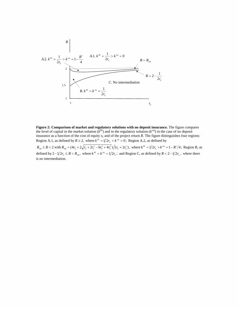
Figure 2: Comparison of market and regulatory solutions with no deposit insurance. The figure compares the level of capital in the market solution (kBS) and in the regulatory solution (kreg) in the case of no deposit insurance as a function of the cost of equity rE and of the project return R. The figure distinguishes four regions: Region A.1, as defined by 2,R ≥ where 1 2 0;BS reg

Ek r k= > = Region A.2, as defined by

2ABR R≤ < with 2 3 4 2(4 2 2 6 4 ) ( 2 ) ,AB E E E E E E ER r r r r r r r= + + − + + where 21 2 1 4;BS regEk r k R= > = − Region B, as

defined by 2 1 2 ,E ABr R R− ≤ < where 1 2 ;BS regEk k r= = and Region C, as defined by 2 1 2 ,ER r< − where there

is no intermediation.

E Er

R

2

21 .2. 12 4

BS reg

E

RA k kr

= > = −

1.1. 02

BS reg

E

A k kr

= > =

C. No intermediation 1.5

1 . 2

BS reg

E

B k kr

= =

122 E

Rr

= −

ABR R=

1

1

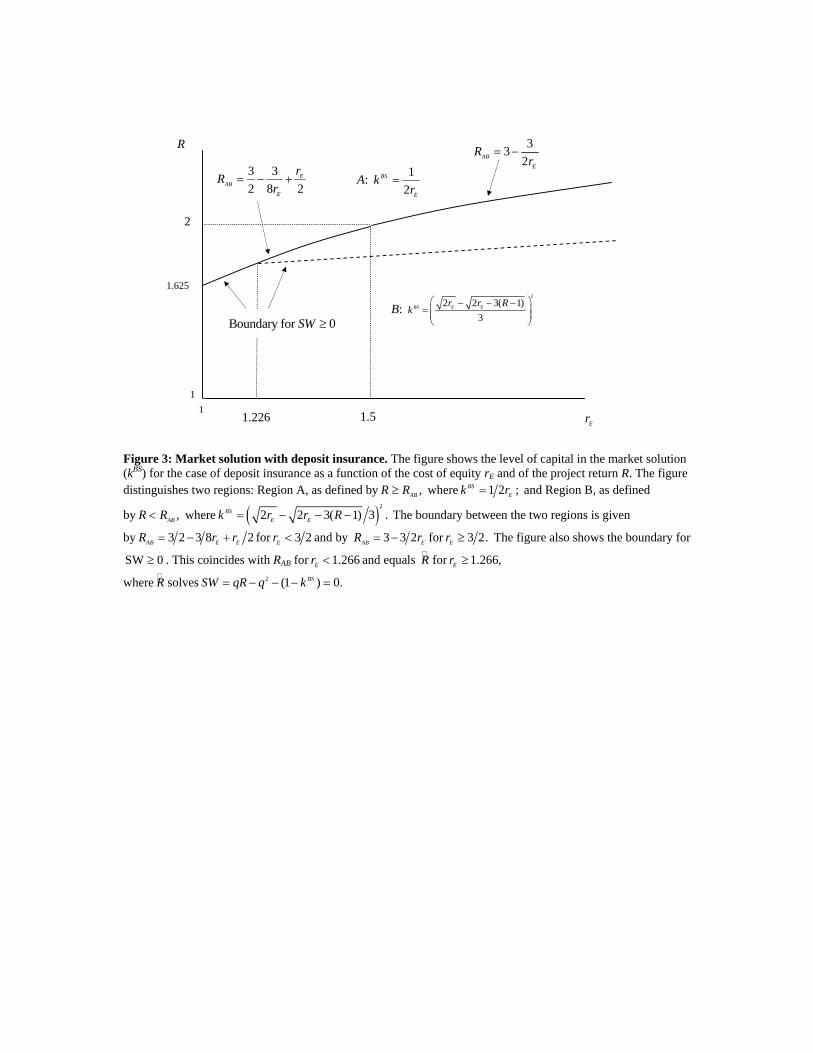
Figure 3: Market solution with deposit insurance. The figure shows the level of capital in the market solution (kBS) for the case of deposit insurance as a function of the cost of equity rE and of the project return R. The figure distinguishes two regions: Region A, as defined by ,ABR R≥ where 1 2 ;BS

Ek r= and Region B, as defined

by ,ABR R< where ( )2

2 2 3( 1) 3 .BSE Ek r r R= − − − The boundary between the two regions is given

by 3 2 3 8 2AB E ER r r= − + for 3 2Er < and by 3 3 2AB ER r= − for 3 2.Er ≥ The figure also shows the boundary for

SW 0≥ . This coincides with RAB for 1.266Er < and equals R for 1.266,Er ≥

where R solves 2 (1 ) 0.BSSW qR q k= − − − =

R

Er 1.5

2

A: 12

BS

E

kr

=

332AB

E

Rr

= −

B: 2

2 2 3( 1)3

BS E Er r Rk

⎛ ⎞− − −= ⎜ ⎟⎜ ⎟⎝ ⎠

3 32 8 2

EAB

E

rR

r= − +

1

1

1.625

1.226

Boundary for 0SW ≥

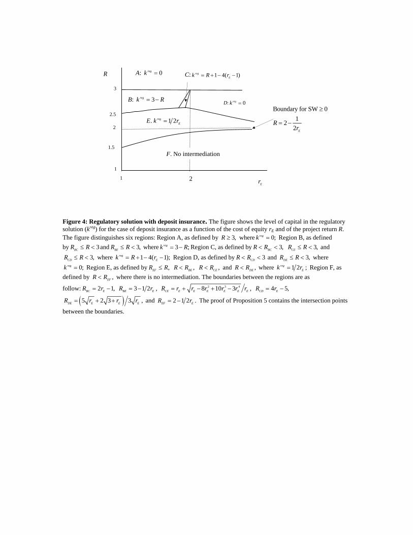
Figure 4: Regulatory solution with deposit insurance. The figure shows the level of capital in the regulatory solution (kreg) for the case of deposit insurance as a function of the cost of equity rE and of the project return R. The figure distinguishes six regions: Region A, as defined by 3,R ≥ where 0;regk = Region B, as defined by 3BCR R≤ < and 3,BER R≤ < where 3 ;regk R= − Region C, as defined by 3,BCR R< < 3,CER R≤ < and

3,CDR R≤ < where 1 4( 1);regEk R r= + − − Region D, as defined by 3CDR R< < and 3,DER R≤ < where

0;regk = Region E, as defined by ,EFR R≤ ,BER R< ,CER R< and ,DER R< where 1 2 ;regEk r= Region F, as

defined by ,EFR R< where there is no intermediation. The boundaries between the regions are as

follow: 2 1,BC ER r= − 3 1 2 ,BE ER r= − 2 3 48 10 3 ,CE E E E E E ER r r r r r r= + − + − 4 5,CD ER r= −

( )5 2 3 3 ,DE E E ER r r r= + + and 2 1 2 .EF ER r= − The proof of Proposition 5 contains the intersection points

between the boundaries.

E Er

R

3

2

2.5 . 1 2reg

EE k r=

B: 3= −regk R D: 0regk =

A: 0regk = C: 1 4( 1)regEk R r= + − −

1.5

Boundary for SW 012

2 E

Rr

≥

= −

F. No intermediation

1

1

2

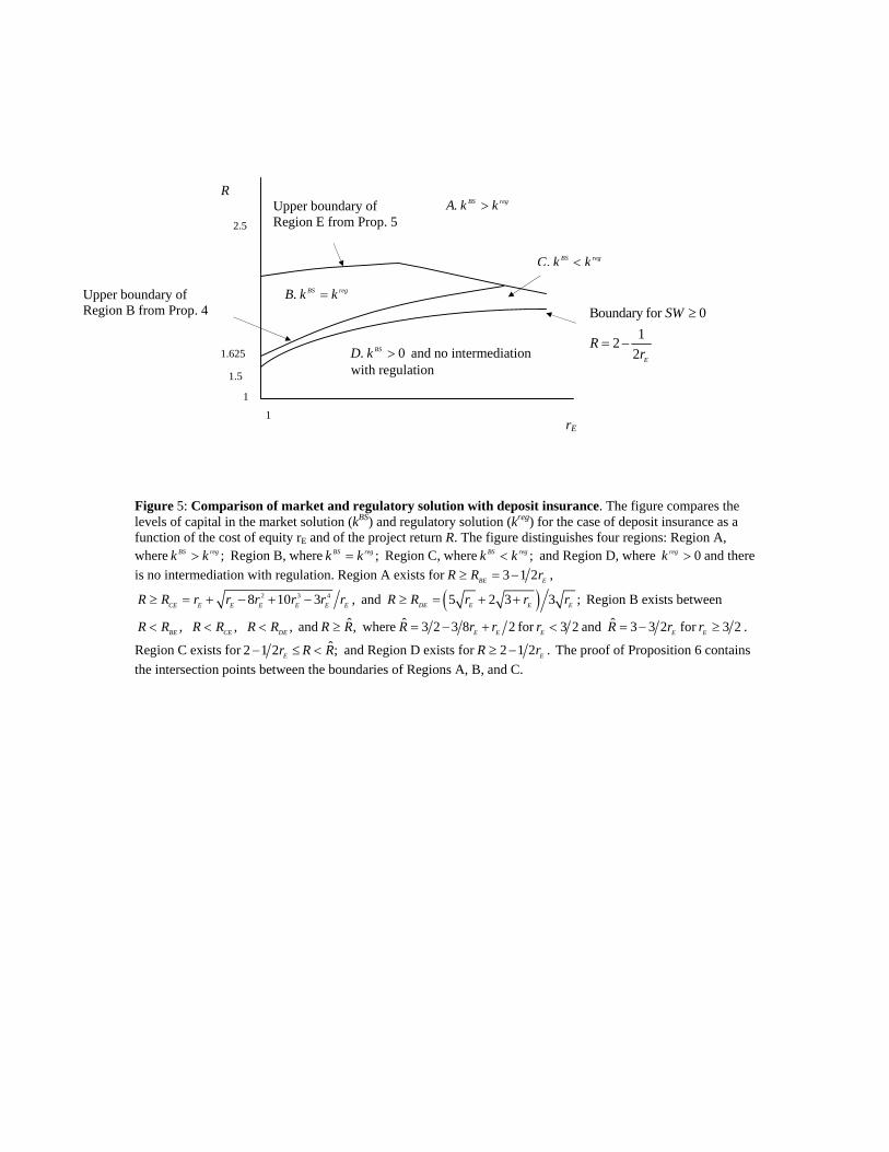
Figure 5: Comparison of market and regulatory solution with deposit insurance. The figure compares the levels of capital in the market solution (kBS) and regulatory solution (kreg) for the case of deposit insurance as a function of the cost of equity rE and of the project return R. The figure distinguishes four regions: Region A, where ;BS regk k> Region B, where ;BS regk k= Region C, where ;BS regk k< and Region D, where 0regk > and there is no intermediation with regulation. Region A exists for 3 1 2 ,BE ER R r≥ = −

2 3 48 10 3 ,CE E E E E E ER R r r r r r r≥ = + − + − and ( )5 2 3 3 ;DE E E ER R r r r≥ = + + Region B exists between

,BER R< ,CER R< ,DER R< and ˆ,R R≥ where ˆ 3 2 3 8 2E ER r r= − + for 3 2Er < and ˆ 3 3 2 ER r= − for 3 2Er ≥ .

Region C exists for ˆ2 1 2 ;Er R R− ≤ < and Region D exists for 2 1 2 .ER r≥ − The proof of Proposition 6 contains the intersection points between the boundaries of Regions A, B, and C.

rE

R

2.5

. BS regC k k<

. BS regA k k>

. BS regB k k=

Upper boundary of Region E from Prop. 5

1.5

1.625 . 0BSD k > and no intermediation with regulation

1

1

Boundary for 012

2 E

SW

Rr

≥

= −

Upper boundary of Region B from Prop. 4