Embed Size (px)
Citation preview
217 Life Sciences Building Bowling Green, OH 43403-0208
419-372-2332 Fax 419-372-2024
www.bgsu.edu/departments/biology
Department of Biological Sciences
18 October, 2011 Ohio Lake Erie Commission, Lake Erie Protection Fund, One Maritime Plaza, Fourth Floor, Toledo, OH 43604-1866 Dear Executive Director Hesse, I submit my Final Report corresponding to LEPF grant SG 389-11, “Credible Data Collection by the U.S. Coast Guard” for your consideration. The Final Report details a research and monitoring partnership with the U.S. Coast Guard which could serve as a model for future monitoring efforts thereby increasing both spatial and temporal resolution of environmental monitoring in the Great Lakes and coastal oceans. As state-funded monitoring programs have been reduced, we have become increasingly reliant on volunteer monitoring programs to help fill the gaps. The collaboration described, while focused seasonally on the study of winter limnology in the Laurentian Great Lakes, could be extended throughout the year. The report addresses each of the components required of the LEPF Final Report including a Technical Report, Final Accounting and an Abstract. Please note that the text comprising the Technical Report has been submitted for consideration to be published as a “Brief report” in the weekly periodical: Eos, Transactions, American Geophysical Union. It is still under review, however, should it be accepted for publication, I will forward a copy of the published article to the Ohio Lake Erie Commission. Thank you for your continued support. Yours sincerely,
Robert Michael L. McKay Ryan Professor of Biology Tel: 419-372-6873 Email: [email protected]
Credible Data Collection by the U.S. Coast Guard Final Report: October 2011 Lake Erie Protection Fund grant SG 398-11 Principal Investigator: Robert Michael L. McKay, Ph.D. Department of Biological Sciences Bowling Green State University
Abstract
Ice-breaking capabilities of the U.S. Coast Guard (USCG) render their vessels safe and reliable
platforms for monitoring and research on ice-covered coastal seas. Since 2009, we have
collaborated with the Commanding Officer and crew of the USCGC NEAH BAY (WTGB 105)
to investigate winter biogeochemistry in Lake Erie. Adopting sampling guidelines of the Ohio
EPA, this collaboration offers potential to develop into a sustainable monitoring program for
which data are contributed to the Ohio Credible Data Program (OCDP). Collaborative efforts
such as this increase monitoring capacity despite continuing federal- and state-government
budgetary restraints.
Ice-breaking capabilities of the U.S. Coast Guard (USCG) render their vessels safe and reliable
platforms for monitoring and research on ice-covered coastal seas. Since 2009, we have
collaborated with the Commanding Officer and crew of the USCGC NEAH BAY (WTGB 105) to
investigate winter biogeochemistry in Lake Erie [McKay et al., 2011]. Adopting sampling
guidelines of the state EPA - the objective of our successful Lake Erie Protection Fund proposal -
this collaboration offers potential to develop into a sustainable monitoring program for which
data are contributed to the Ohio Credible Data Program (OCDP). Collaborative efforts such as
this increase monitoring capacity despite continuing federal- and state-government budgetary
restraints.
Lake Erie boasts multi-billion dollar fisheries and a vibrant tourism industry. The watershed
spans parts of the Canadian province of Ontario and five American states and supports a
population of 12 million. Consistent with the lake’s small volume, ice cover is extensive in
winter. Dangers inherent with shifting ice floes result in much of Lake Erie becoming
inaccessible, hindering winter research and monitoring.
Winter presents a logistical barrier to better understanding the lake ecosystem, and current trends
in global climate warming provide cause for establishing in-depth baseline measurements during
winter in the Great Lakes. Addressing these issues, USCG operations on Lake Erie facilitate
monitoring. Operation Coal Shovel, authorized by provisions in Title 14 of the U.S. Code,
mandates USCG icebreaking activities to facilitate commercial shipping traffic driven by the
year-round demands of industry in the Lake Erie basin. Logistical considerations generally
prevent researchers from being embedded on-board NEAH BAY; however, crew members under
supervision of the Commanding Officer were trained to collect and process samples during
routine operations.
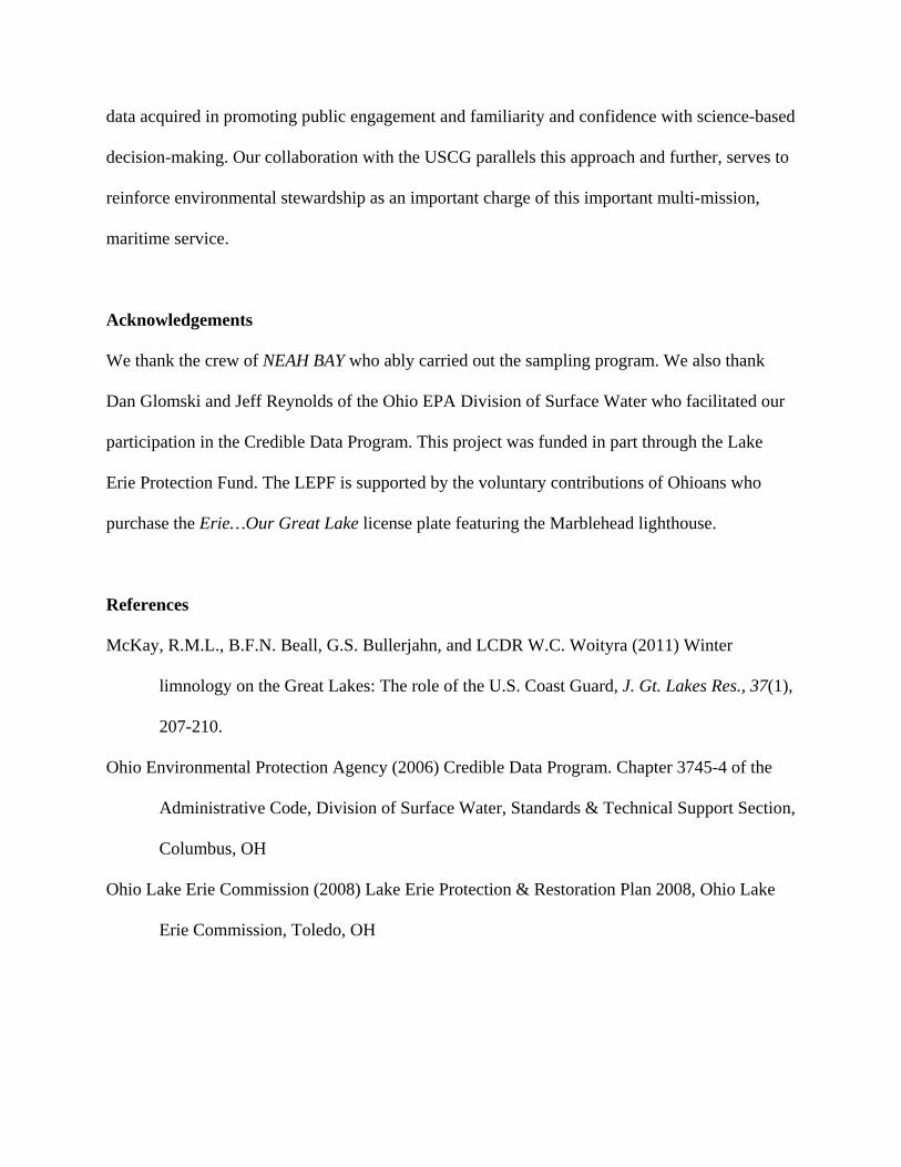
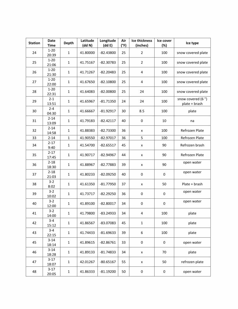
During winter 2010-2011, the monitoring effort included synoptic sampling of surface waters of
Lake Erie conducted during normal operations of NEAH BAY from November through March
(Fig. 1). When possible, water samples were collected at hourly intervals while underway to
provide a spatial and temporal survey for algal biomass (as chlorophyll [chl] a), dissolved- and
particulate nutrients and other physicochemical parameters (see Appendix I for results).
The role of community volunteers in water quality monitoring is growing, yet differing
methodologies introduce inconsistency into data and the resulting inter-study variability
complicates accurate synthesis of these efforts. Addressing these inherent differences, Amended
House Bill 43 created the OCDP in 2003 (Ohio EPA, 2006). Ohio’s “credible data law” (sections
6111.50 to 6111.56 of the Ohio Revised Code) sets standards for data collection practices.
Integrating winter monitoring into the framework of the OCDP ensured that the guidelines for
the standardization of water quality assessments were followed.
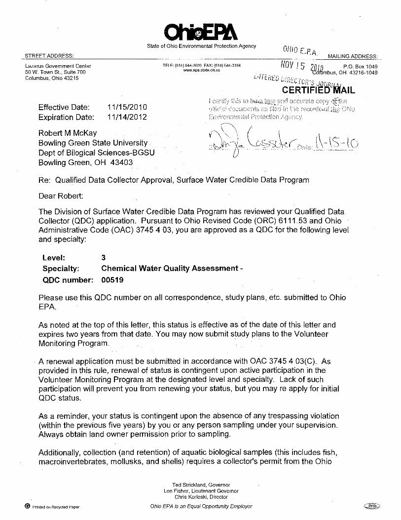
In order to participate in the OCDP, investigators were certified as Qualified Data Collectors
(QDC) for Chemical Water Quality Assessment (Appendix II) and study plans were submitted
for approval by the Ohio EPA (Appendix III). EPA personnel oversaw training sessions for crew
of NEAH BAY prior to commencement of the monitoring project promoting adherence to
Credible Data collection requirements. USCG servicemen conducted all sample collection under
the direct supervision of a QDC.
Data collected through the OCDP is categorized into three levels based on the qualifications of
the collector and the sophistication of collection methods. Each level of data may in turn be used
for varying purposes. Level 1 data is intended primarily for promoting public awareness and
stewardship whereas Level 2 data may be used to assess efficacy of pollution control. Level 3
data is collected using the most stringent methods and may be used for all purposes defined for
Levels 1 and 2 data as well as for regulatory purposes specified in the Ohio Revised Code.
A strategic objective of the 2008 Lake Erie Protection and Restoration Plan calls for the
“expansion of citizen stewardship programs, including volunteer monitoring, throughout the
watershed” [Ohio Lake Erie Commission, 2008]. Although credible data programs provide the
framework for scientifically sound monitoring, volunteers are often limited in their monitoring
capabilities. The USCG has unique capabilities making them especially adept for aquatic
monitoring. Melding the OCDP with current USCG operations affords a high quality data
acquisition system whilst still fulfilling USCG obligations to Operation Coal Shovel.
NEAH BAY is one of several Coast Guard vessels involved in winter operations on the Great
Lakes which include contributions from the Canadian Coast Guard and its Icebreaking Program.
Expansion of sampling to include other vessels is a future objective. Parallel state-managed
credible data programs existing throughout the U.S. offer similar opportunities for USCG
cooperation. The benefits of developing non-scientist monitoring programs extend beyond the
data acquired in promoting public engagement and familiarity and confidence with science-based
decision-making. Our collaboration with the USCG parallels this approach and further, serves to
reinforce environmental stewardship as an important charge of this important multi-mission,
maritime service.
Acknowledgements
We thank the crew of NEAH BAY who ably carried out the sampling program. We also thank
Dan Glomski and Jeff Reynolds of the Ohio EPA Division of Surface Water who facilitated our
participation in the Credible Data Program. This project was funded in part through the Lake
Erie Protection Fund. The LEPF is supported by the voluntary contributions of Ohioans who
purchase the Erie…Our Great Lake license plate featuring the Marblehead lighthouse.
References
McKay, R.M.L., B.F.N. Beall, G.S. Bullerjahn, and LCDR W.C. Woityra (2011) Winter
limnology on the Great Lakes: The role of the U.S. Coast Guard, J. Gt. Lakes Res., 37(1),
207-210.
Ohio Environmental Protection Agency (2006) Credible Data Program. Chapter 3745-4 of the
Administrative Code, Division of Surface Water, Standards & Technical Support Section,
Columbus, OH
Ohio Lake Erie Commission (2008) Lake Erie Protection & Restoration Plan 2008, Ohio Lake
Erie Commission, Toledo, OH
Fig. 1. Winter season 2010-2011 navigation tracks of USCGC NEAH BAY (blue) demonstrate
monitoring potential in Lake Erie by partnering with the U.S. Coast Guard. Sampling was
conducted at 48 sites between November – March. The Ninth Coast Guard District is home to 9
ice-breaking cutters whose operations cover the 5 Great Lakes and the St. Lawrence Seaway
offering further opportunities to conduct monitoring.
APPENDIX I Monitoring Results
Materials and Methods
Sampling:
The sampling protocol was designed to capture the spatial and temporal distribution of size
fractionated chlorophyll (chl)-a biomass with accompanying nutrient concentrations from
surface waters during winter 2010-2011. Sampling was conducted by personnel of the USCGC
NEAH BAY from November, 2010 through March, 2011. Samples were collected and processed
on board NEAH BAY by crewmembers under the supervision of a Level 3 QDC and following
protocols detailed in the attached approved Study Plan (Appendix III).
Chl a:
Sampling for size-fractionated chl-a was conducted at 47 stations over the winter period. Size-
fractions included total chl-a and the microplankton size fraction. Total chl was processed using
glass fiber filters (GF/F) and polycarbonate (PCTE) filters of 0.2 µm pore-size whereas the
microplankton were fractionated using 20 µm PCTE membranes. Following vacuum filtration,
filters were placed in a polyethylene tube and stored at -20 °C. Samples were transported to
BGSU for extraction and analysis. Extraction followed protocol LG405, developed by the EPA’s
Great Lakes National Program Office (GLNPO) for water quality surveys of the Great Lakes
(Appendix III).
Nutrients:
Nutrient analysis was conducted for 31 stations starting in December, 2010. For nutrient
analysis, samples were processed for analysis by either Heidelberg University (National Center
for Water Quality Research) or the Ohio EPA. Samples for dissolved nutrient analysis at
Heidelberg were filtered (< 0.22 µm) into acid-cleaned HDPE bottles prior to freezing. Samples
for analysis by Ohio EPA were acidified with sulfuric acid following the procedures described in
Appendix III.
Results
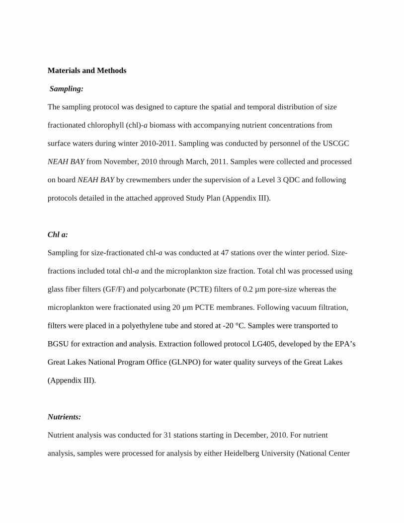
Our data suggest that winter phytoplankton biomass in Lake Erie is both spatially and temporally
dynamic (Fig. 2). Total chl concentrations ranged from 0.1 µg L-1 (December) to 84.7 µg L-1
(March). Average monthly total chl ranged from 1.2 µg L-1 in December, to 18.8 µg L-1 in
March. Microplankton (> 20 µm) dominated total chl starting in January comprising > 70% of
total chl. Microplankton dominance remained high for the remainder of the winter, plateauing in
February.
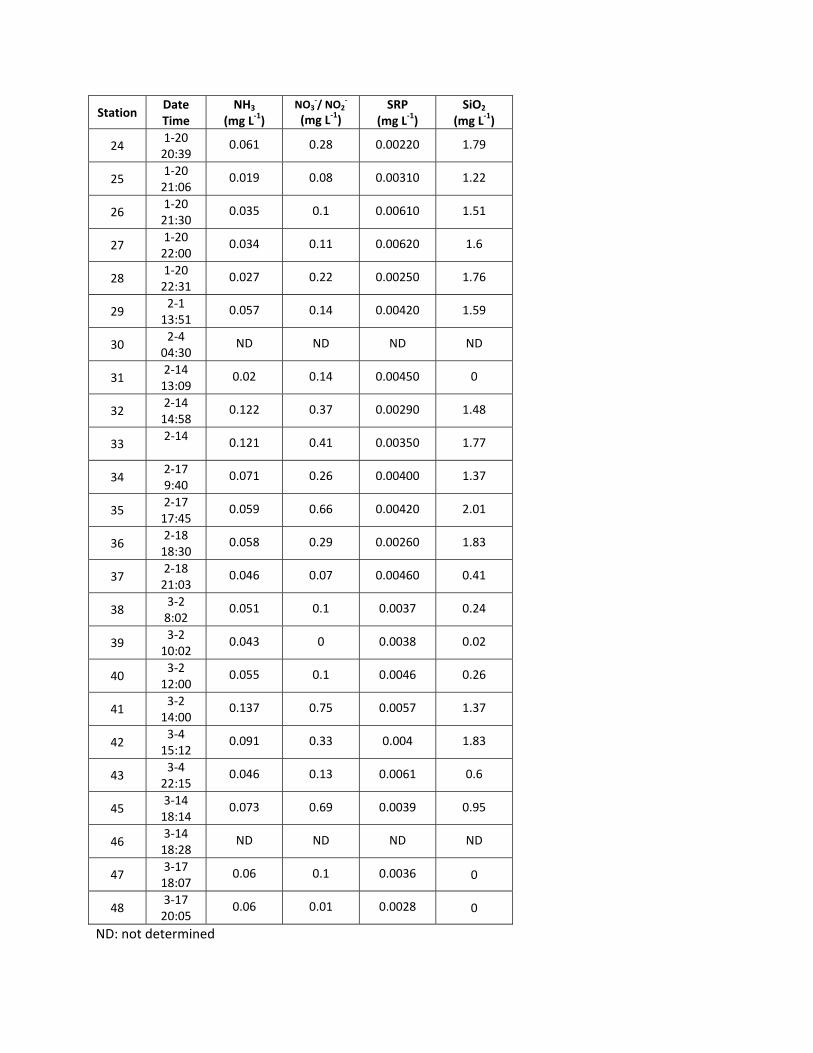
Ammonium, nitrate/nitrite, silicic acid and soluble reactive phosphorus (SRP) were analyzed at
31 stations between December, 2010 to March, 2011. A seasonal depletion in silica levels was
consistent with greater intensity of diatom blooms as the season progressed. Early winter
(December) silica levels ranged from 1.51 mg L-1 – 2.32 mg L-1. By March, levels had become
depleted completely at some sites. Silica varied spatially as well with higher levels in the western
basin compared to elsewhere in the lake. Likewise, nitrate levels displayed spatial variability
decreasing from west to east of the Lake Erie islands. Nitrate levels, however, did not appear to
decrease temporally from early- to late winter. SRP levels were elevated throughout the winter
with no spatial trends.
Fig. 2. Spatial- and temporal variability of chl a biomass sampled
by USCGC NEAH BAY between November, 2010 – March, 2011.
Data are divided between early winter (Nov – Jan; red) and late
winter (Feb – March; black). Range of concentrations (µg L-1) of
chl a are shown in legend at right.
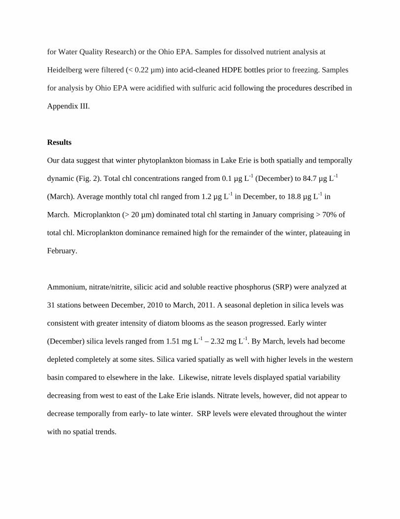
Station Date Time
Depth Latitude (dd N)
Longitude(dd E)
Air(°F)
Ice thickness (inches)
Ice cover (%)
Ice type
1 11‐08 10:05
1 41.63233 ‐81.99333 54 0 0 open water
2 11‐08 12:00
1 41.75400 ‐82.24750 52 0 0 open water
3 11‐08 1:01
1 41.84033 ‐82.52467 49 0 0 open water
4 11‐08 2:00
1 41.88633 ‐82.73800 38 0 0 open water
5 11‐11 11:00
1 41.93383 ‐82.03383 50 0 0 open water
6 11‐11 12:00
1 41.89000 ‐82.79717 53 0 0 open water
7 11‐11 13:00
1 41.85733 ‐82.56417 59 0 0 open water
8 11‐11 14:00
1 41.77317 ‐82.35167 59 0 0 open water
9 11‐11 15:00
1 41.76133 ‐82.13583 60 0 0 open water
10 11‐11 17:10
1 41.74817 ‐81.69717 60 0 0 open water
11 12‐09 11:50
1 41.74817 ‐81.69717 30 0 0 open water
12 12‐22 14:00
1 41.70083 ‐83.14483 32 4 100 plate
13 12‐22 16:00
1 41.87717 ‐83.20350 35 3 100 plate
14 12‐23 08:30
1 41.89233 ‐82.81583 32 4 100 plate
15 12‐23 11:20
1 41.63583 ‐82.10733 34 0 0 open water
16 12‐26 13:25
1 41.88617 ‐82.73183 25 6 90 plate
17 12‐26 16:35
1 41.88950 ‐83.11583 30 6 100 refrozen brash
18 12‐27 12:00
1 41.83400 ‐83.07317 28 x 100 refrozen brash
19 12‐28 10:07
1 41.81517 ‐83.01117 22 x 80 refrozen brash
20 12‐29 11:42
1 41.90300 ‐82.96750 32 x 90 refrozen brash,
windrows, pancake
21 12‐29 12:47
1 41.88083 ‐82.70950 37 x 80 refrozen brash
22 12‐29 17:00
1 41.76283 ‐83.13700 30 x 30 frozen Plate
23a 12‐30 14:30
1 41.71750 ‐81.69583 39 0 0 open water
23b 12‐30 14:30
1 41.71750 ‐81.69583 39 0 0 open water
Station Date Time
Depth Latitude (dd N)
Longitude(dd E)
Air(°F)
Ice thickness (inches)
Ice cover (%)
Ice type
24 1‐20 20:39
1 41.80000 ‐82.43800 25 2 100 snow covered plate
25 1‐20 21:06
1 41.75167 ‐82.30783 25 2 100 snow covered plate
26 1‐20 21:30
1 41.71267 ‐82.20483 25 4 100 snow covered plate
27 1‐20 22:00
1 41.67650 ‐82.10800 25 4 100 snow covered plate
28 1‐20 22:31
1 41.64083 ‐82.00800 25 24 100 snow covered plate
29 2‐1 13:51
1 41.65967 ‐81.71350 24 24 100 snow covered (6 ")
plate + brash
30 2‐4 04:30
1 41.66667 ‐81.92917 30 8.5 100 plate
31 2‐14 13:09
1 41.79183 ‐82.42117 40 0 10 na
32 2‐14 14:58
1 41.88383 ‐82.73300 36 x 100 Refrozen Plate
33 2‐14 1 41.90550 ‐82.97017 36 5 100 Refrozen Plate
34 2‐17 9:40
1 41.54700 ‐82.65517 45 x 90 Refrozen brash
35 2‐17 17:45
1 41.90717 ‐82.94967 44 x 90 Refrozen Plate
36 2‐18 18:30
1 41.88967 ‐82.77883 39 x 90 open water
37 2‐18 21:03
1 41.80233 ‐82.09250 40 0 0 open water
38 3‐2 8:02
1 41.61350 ‐81.77950 37 x 50 Plate + brash
39 3‐2 10:02
1 41.73717 ‐82.29250 36 0 0 open water
40 3‐2 12:00
1 41.89100 ‐82.80017 34 0 0 open water
41 3‐2 14:00
1 41.79800 ‐83.24933 34 4 100 plate
42 3‐4 15:12
1 41.86567 ‐83.07083 45 1 100 plate
43 3‐4 22:15
1 41.74433 ‐81.69633 39 6 100 plate
45 3‐14 18:14
1 41.89615 ‐82.86761 33 0 0 open water
46 3‐14 18:28
1 41.89133 ‐81.74833 34 x 70 plate
47 3‐17 18:07
1 42.01267 ‐80.65167 55 x 50 refrozen plate
48 3‐17 20:05
1 41.86333 ‐81.19200 50 0 0 open water
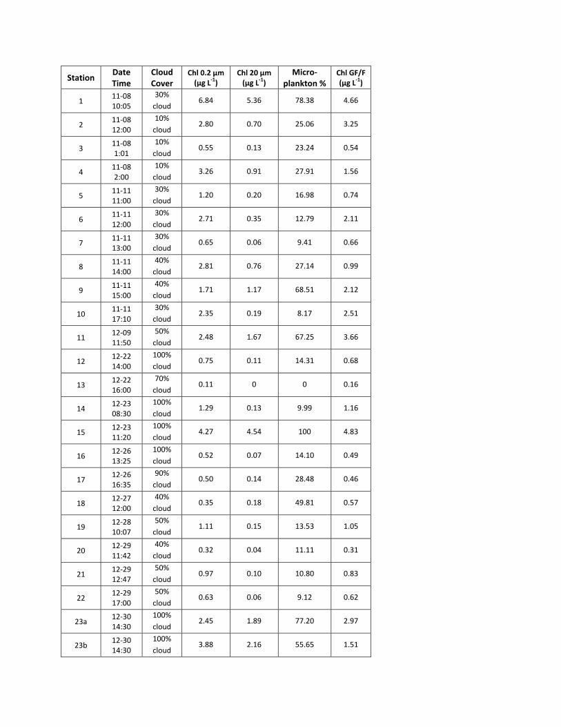
Station Date Time
Cloud Cover
Chl 0.2 µm (µg L‐1)
Chl 20 µm (µg L‐1)
Micro‐plankton %
Chl GF/F (µg L‐1)
1 11‐08 10:05
30% cloud
6.84 5.36 78.38 4.66
2 11‐08 12:00
10% cloud
2.80 0.70 25.06 3.25
3 11‐08 1:01
10% cloud
0.55 0.13 23.24 0.54
4 11‐08 2:00
10% cloud
3.26 0.91 27.91 1.56
5 11‐11 11:00
30% cloud
1.20 0.20 16.98 0.74
6 11‐11 12:00
30% cloud
2.71 0.35 12.79 2.11
7 11‐11 13:00
30% cloud
0.65 0.06 9.41 0.66
8 11‐11 14:00
40% cloud
2.81 0.76 27.14 0.99
9 11‐11 15:00
40% cloud
1.71 1.17 68.51 2.12
10 11‐11 17:10
30% cloud
2.35 0.19 8.17 2.51
11 12‐09 11:50
50% cloud
2.48 1.67 67.25 3.66
12 12‐22 14:00
100% cloud
0.75 0.11 14.31 0.68
13 12‐22 16:00
70% cloud
0.11 0 0 0.16
14 12‐23 08:30
100% cloud
1.29 0.13 9.99 1.16
15 12‐23 11:20
100% cloud
4.27 4.54 100 4.83
16 12‐26 13:25
100% cloud
0.52 0.07 14.10 0.49
17 12‐26 16:35
90% cloud
0.50 0.14 28.48 0.46
18 12‐27 12:00
40% cloud
0.35 0.18 49.81 0.57
19 12‐28 10:07
50% cloud
1.11 0.15 13.53 1.05
20 12‐29 11:42
40% cloud
0.32 0.04 11.11 0.31
21 12‐29 12:47
50% cloud
0.97 0.10 10.80 0.83
22 12‐29 17:00
50% cloud
0.63 0.06 9.12 0.62
23a 12‐30 14:30
100% cloud
2.45 1.89 77.20 2.97
23b 12‐30 14:30
100% cloud
3.88 2.16 55.65 1.51
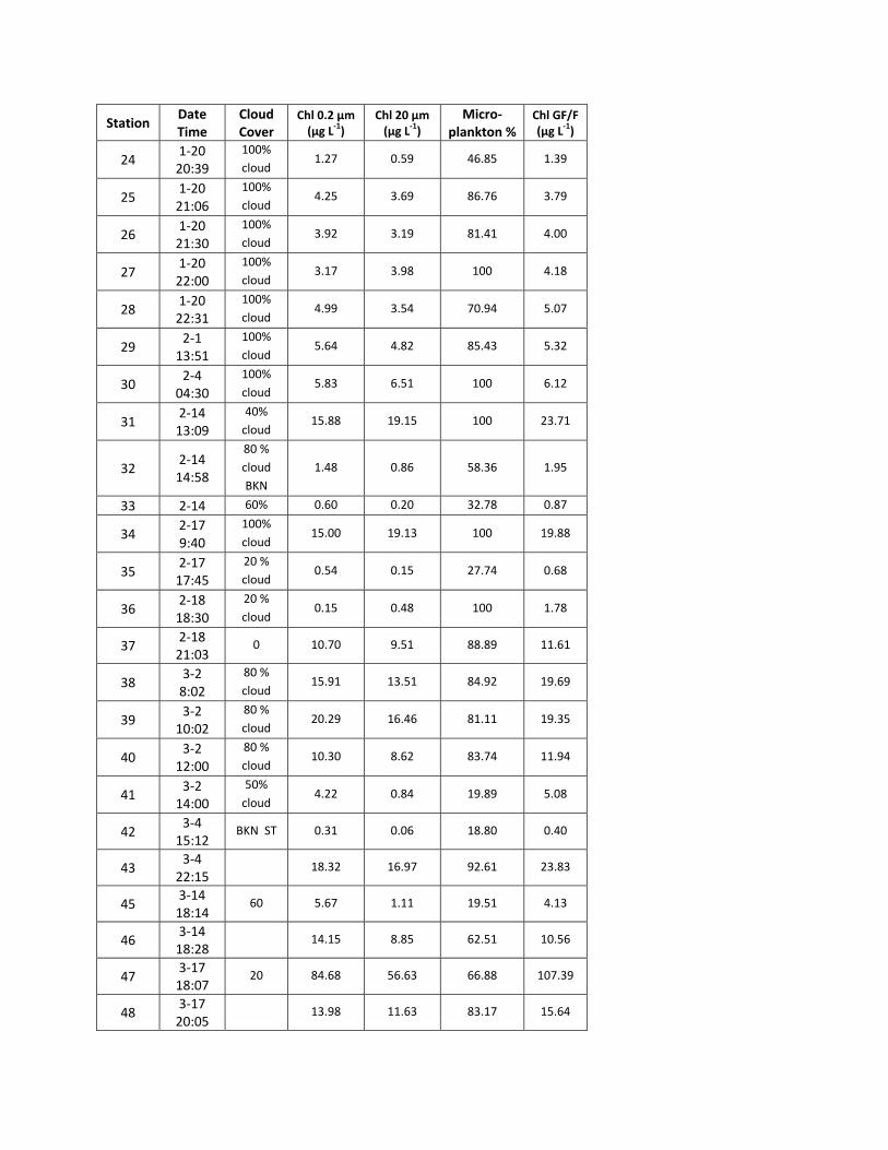
Station Date Time
Cloud Cover
Chl 0.2 µm (µg L‐1)
Chl 20 µm (µg L‐1)
Micro‐plankton %
Chl GF/F (µg L‐1)
24 1‐20 20:39
100% cloud
1.27 0.59 46.85 1.39
25 1‐20 21:06
100% cloud
4.25 3.69 86.76 3.79
26 1‐20 21:30
100% cloud
3.92 3.19 81.41 4.00
27 1‐20 22:00
100% cloud
3.17 3.98 100 4.18
28 1‐20 22:31
100% cloud
4.99 3.54 70.94 5.07
29 2‐1 13:51
100% cloud
5.64 4.82 85.43 5.32
30 2‐4 04:30
100% cloud
5.83 6.51 100 6.12
31 2‐14 13:09
40% cloud
15.88 19.15 100 23.71
32 2‐14 14:58
80 % cloud BKN
1.48 0.86 58.36 1.95
33 2‐14 60% 0.60 0.20 32.78 0.87
34 2‐17 9:40
100% cloud
15.00 19.13 100 19.88
35 2‐17 17:45
20 % cloud
0.54 0.15 27.74 0.68
36 2‐18 18:30
20 % cloud
0.15 0.48 100 1.78
37 2‐18 21:03
0 10.70 9.51 88.89 11.61
38 3‐2 8:02
80 % cloud
15.91 13.51 84.92 19.69
39 3‐2 10:02
80 % cloud
20.29 16.46 81.11 19.35
40 3‐2 12:00
80 % cloud
10.30 8.62 83.74 11.94
41 3‐2 14:00
50% cloud
4.22 0.84 19.89 5.08
42 3‐4 15:12
BKN ST 0.31 0.06 18.80 0.40
43 3‐4 22:15
18.32 16.97 92.61 23.83
45 3‐14 18:14
60 5.67 1.11 19.51 4.13
46 3‐14 18:28
14.15 8.85 62.51 10.56
47 3‐17 18:07
20 84.68 56.63 66.88 107.39
48 3‐17 20:05
13.98 11.63 83.17 15.64
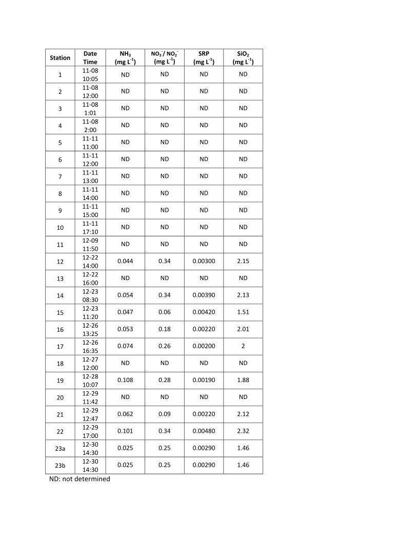
Station Date Time
NH3 (mg L‐1)
NO3‐/ NO2
‐ (mg L‐1)
SRP(mg L‐1)
SiO2
(mg L‐1)
1 11‐08 10:05
ND ND ND ND
2 11‐08 12:00
ND ND ND ND
3 11‐08 1:01
ND ND ND ND
4 11‐08 2:00
ND ND ND ND
5 11‐11 11:00
ND ND ND ND
6 11‐11 12:00
ND ND ND ND
7 11‐11 13:00
ND ND ND ND
8 11‐11 14:00
ND ND ND ND
9 11‐11 15:00
ND ND ND ND
10 11‐11 17:10
ND ND ND ND
11 12‐09 11:50
ND ND ND ND
12 12‐22 14:00
0.044 0.34 0.00300 2.15
13 12‐22 16:00
ND ND ND ND
14 12‐23 08:30
0.054 0.34 0.00390 2.13
15 12‐23 11:20
0.047 0.06 0.00420 1.51
16 12‐26 13:25
0.053 0.18 0.00220 2.01
17 12‐26 16:35
0.074 0.26 0.00200 2
18 12‐27 12:00
ND ND ND ND
19 12‐28 10:07
0.108 0.28 0.00190 1.88
20 12‐29 11:42
ND ND ND ND
21 12‐29 12:47
0.062 0.09 0.00220 2.12
22 12‐29 17:00
0.101 0.34 0.00480 2.32
23a 12‐30 14:30
0.025 0.25 0.00290 1.46
23b 12‐30 14:30
0.025 0.25 0.00290 1.46
ND: not determined
Station Date Time
NH3 (mg L‐1)
NO3‐/ NO2
‐ (mg L‐1)
SRP(mg L‐1)
SiO2
(mg L‐1)
24 1‐20 20:39
0.061 0.28 0.00220 1.79
25 1‐20 21:06
0.019 0.08 0.00310 1.22
26 1‐20 21:30
0.035 0.1 0.00610 1.51
27 1‐20 22:00
0.034 0.11 0.00620 1.6
28 1‐20 22:31
0.027 0.22 0.00250 1.76
29 2‐1 13:51
0.057 0.14 0.00420 1.59
30 2‐4 04:30
ND ND ND ND
31 2‐14 13:09
0.02 0.14 0.00450 0
32 2‐14 14:58
0.122 0.37 0.00290 1.48
33 2‐14
0.121 0.41 0.00350 1.77
34 2‐17 9:40
0.071 0.26 0.00400 1.37
35 2‐17 17:45
0.059 0.66 0.00420 2.01
36 2‐18 18:30
0.058 0.29 0.00260 1.83
37 2‐18 21:03
0.046 0.07 0.00460 0.41
38 3‐2 8:02
0.051 0.1 0.0037 0.24
39 3‐2 10:02
0.043 0 0.0038 0.02
40 3‐2 12:00
0.055 0.1 0.0046 0.26
41 3‐2 14:00
0.137 0.75 0.0057 1.37
42 3‐4 15:12
0.091 0.33 0.004 1.83
43 3‐4 22:15
0.046 0.13 0.0061 0.6
45 3‐14 18:14
0.073 0.69 0.0039 0.95
46 3‐14 18:28
ND ND ND ND
47 3‐17 18:07
0.06 0.1 0.0036 0
48 3‐17 20:05
0.06 0.01 0.0028 0
ND: not determined
APPENDIX II Qualified Data Collector
Credentials
State of Ohio Environmental Protection Agency Oi}'{', . 11) t.P.!'....
Lazarus Government Center 50 W. Town St.. Suite 700 Columbus, Ohio 43215
Effective Date: 11/15/2010 Expiration Date: 11/14/2012
Benjamin F Beall Bowling Green State University .\. \\~ \
\ , Ie Dept of Bilogocial Sciences-BGSU Bowling Green, OH 43403
Re: Oualified Data Collector Approval, Surface Water Credible Data Program
Dear Benjamin:
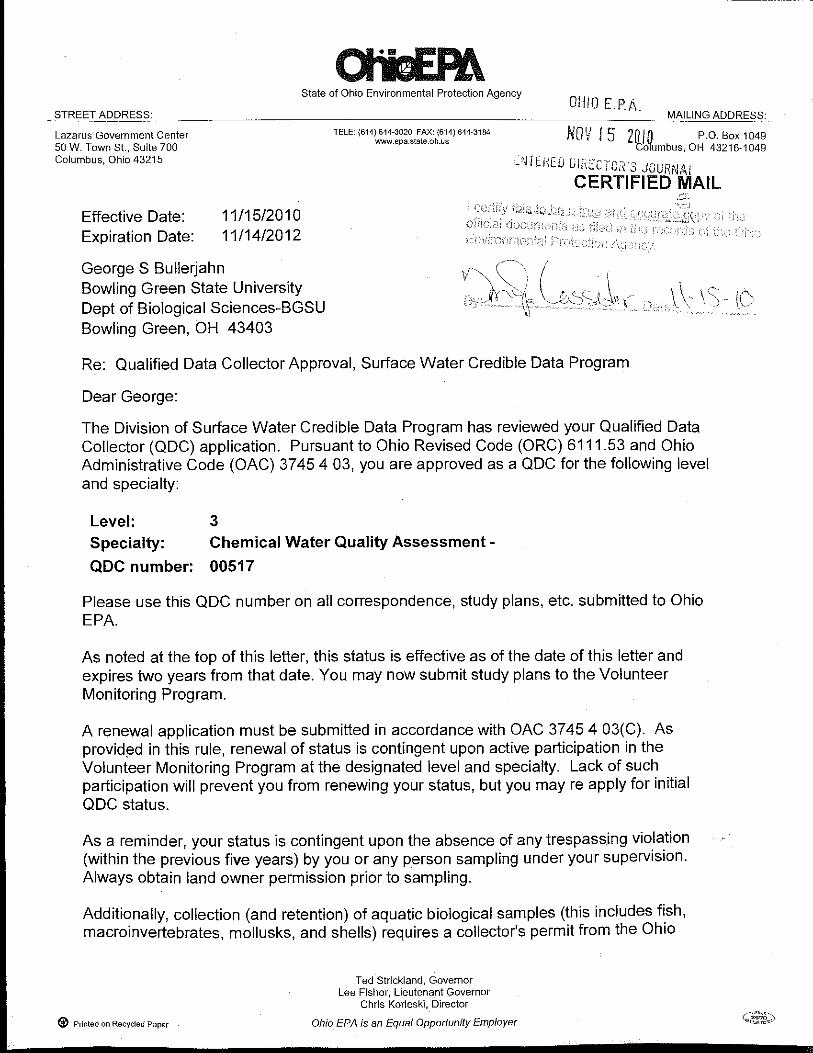
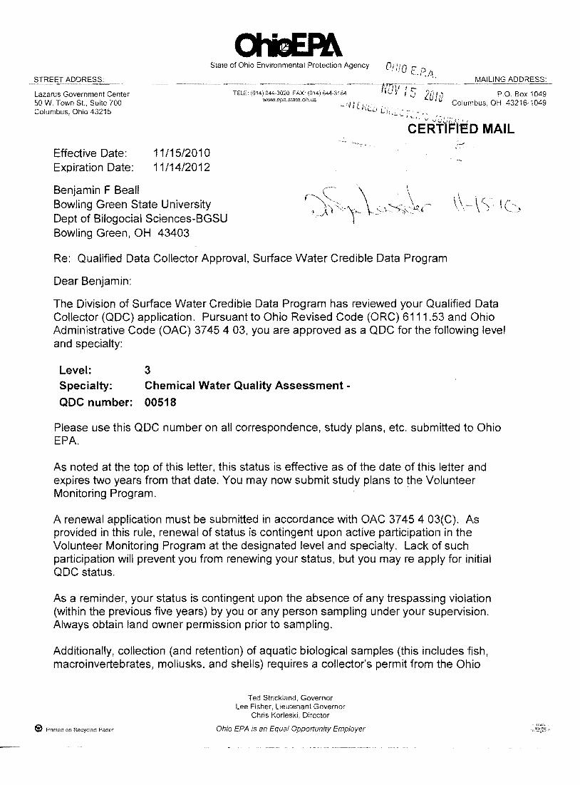
The Division of Surface Water Credible Data Program has reviewed your Oualified Data Collector (ODC) application. Pursuant to Ohio Revised Code (ORC) 6111.53 and Ohio Administrative Code (OAC) 3745 4 03, you are approved as a ODC for the following level and specialty:
Level: 3 Specialty: Chemical Water Quality Assessment
QDC number: 00518
Please use this ODC number on all correspondence, study plans, etc. submitted to Ohio EPA.
As noted at the top of this letter, this status is effective as of the date of this letter and expires two years from that date. You may now submit study plans to the Volunteer Monitoring Program.
A renewal application must be submitted in accordance with OAC 3745 4 03(C). As provided in this rule, renewal of status is contingent upon active participation in the Volunteer Monitoring Program at the designated level and specialty. Lack of such participation will prevent you from renewing your status, but you may re apply for initial ODC status.
As a reminder, your status is contingent upon the absence of any trespassing violation (within the previous five years) by you or any person sampling under your supervision. Always obtain land owner permission prior to sampling.
Additionally, collection (and retention) of aquatic biological samples (this includes fish, macroinvertebrates, mollusks, and shells) requires a collector's permit from the Ohio
Ted Strickland, Governor Lee Fisher, Lieutenant Governor
Chris Korleski, Director
(i) Printed on Recycled Paper Ohio EPA is an Equal Opportunity Employer
Department of Natural Resources/Division of Wildlife. Obtain this permit prior to collection of any biological samples.
You are hereby notified that this action of the Director is final and may be appealed to the Environmental Review Appeals Commission pursuant to Section 3745.04 of the Ohio Revised Code. The appeal must be in writing and set forth the action complained of and the grounds upon which the appeal is based. The appeal must be filed with the Commission within thirty (30) days after notice of the Director's action. The appeal must be accompanied by a filing fee of $70.00, made payable to "Ohio Treasurer Kevin Boyce", which the Commission, in its discretion, may reduce if by affidavit you demonstrate that payment of the full amount of the fee would cause extreme hardship. Notice of the filing of the appeal shall be filed with the Director within three (3) days of filing with the Commission. Ohio EPA requests that a copy of the appeal be served upon the Ohio Attorney General's Office, Environmental Enforcement Section. An appeal may be filed with the Environmental Review Appeals Commission at the following address: Environmental Review Appeals Commission, 309 South Fourth Street, Room 222, Columbus, OH 43215.
Sincerely,
r,
'" ... ~/
hns ores i, . " Director ~~
STREET ADDRESS:
State of Ohio Environmental Protection Agency *i{l 0 f . p. 11 -
MAILING ADDRESS:
Lazarus Government Center50 W. Town St., Suite 700Columbus, Ohio 43215
Effective Date: 1111512010
Expiration Date: 1111412012
Ben OysermanBowling Green State University18 Regent DrAnn Arbor, Ml 48104
TELE: (614) 644-3020 FAX: (614) 644-3184M.epa.state.oh.us fdfiV i 5 |illil Po Box1o4e
Columbus, OH 43216-1049
-:,i lLiierr ti;rIi iGf i JSiiiifi;iiCERTIFIED MAIL
.i:I
9_ertify this to.-Qg-q.tru9, gnd.pqgurate_ cffif tne
official documents as filed in the records oithe Ohi<lEnvironmental Protection Agency.('r t
DNk( ..s=.Ico*.,r.f \S Io
Re: Qualified Data Collector Approval, Surface Water Credible Data Program
Dear Ben:
The Division of Surface Water Credible Data Program has reviewed your Qualified DataCollector (ODC) application. Pursuant to Ohio Revised Code (ORC) 6111.53 and OhioAdministrative Code (OAC) 3745 4 03, you are approved as a QDC for the following level
and specialty:
Levet: 3
Specialty: Chemical Water Quality Assessment -
QDC number: 00520
Please use this QDC number on all correspondence, study plans, etc. submitted to OhioEPA.
As noted at the top of this letter, this status is effective as of the date of this letter andexpires two years from that date. You may now submit study plans to the VolunteerMonitoring Program.
A renewal application must be submitted in accordance with OAC 3745 4 03(C). Asprovided in this rule, renewal of status is contingent upon active participation in theVolunteer Monitoring Program at the designated level and specialty. Lack of suchparticipation will prevent you from renewing your status, but you may re apply for initialQDC status.
As a reminder, your status is contingent upon the absence of any trespassing violation(within the previous five years) by you or any person sampling under your supervision.Always obtain land owner permission prior to sampling.
Additionally, collection (and retention) of aquatic biological samples (this includes fish,macroinvertebrates, mollusks, and shells) requires a collector's permit from the Ohio
Ted Strickland, GovernorLee Fisher, Lieutenant Governor
Chris Korleski, Director
Ohio EPA is an Equal Opportunity Employer@ Print"d on Recycled Paper
Department of Natural Resources/Division of Wildlife. Obtain this permit prior to collection
of any biological samples.
You are hereby notified that this action of the Director is final and may be appealed to the
Environmental Review Appeals Commission pursuant to Section 3745.04 of the Ohio
Revised Code. The appeal must be in writing and set forth the action complained of and
the grounds upon which the appeal is based. The appeal must be filed with theCommission within thirty (30) days after notice of the Director's action. The appeal must
be accompanied by a fiiing fee of $70.00, made payable to "Ohio Treasurer Kevin Boyce",
which the Commission, in its discretion, may reduce if by affidavit you demonstrate thatpayment of the full amount of the fee would cause extreme hardship. Notice of the filing
ot ine appeal shall be filed with the Director within three (3) days of filing with the
Commission. Ohio EPA requests that a copy of the appeal be served upon the Ohio
Attorney General's Office, Environmental Enforcement Section. An appeal may be filed
with the Environmental Review Appeals Commission at the following address:
Environmental Review Appeals Commission, 309 South Fourth Street, Room 222,
Columbus, OH 43215.
Sincerely,&M.Chris Korleski,Director
APPENDIX III Approved Study Plan
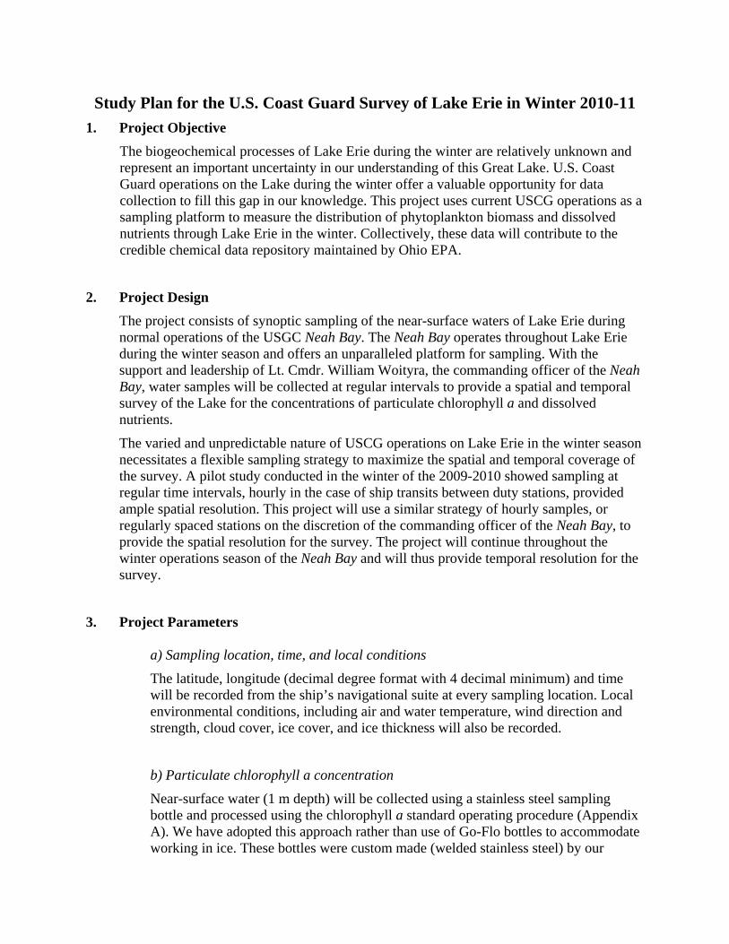
Study Plan for the U.S. Coast Guard Survey of Lake Erie in Winter 2010-11 1. Project Objective
The biogeochemical processes of Lake Erie during the winter are relatively unknown and represent an important uncertainty in our understanding of this Great Lake. U.S. Coast Guard operations on the Lake during the winter offer a valuable opportunity for data collection to fill this gap in our knowledge. This project uses current USCG operations as a sampling platform to measure the distribution of phytoplankton biomass and dissolved nutrients through Lake Erie in the winter. Collectively, these data will contribute to the credible chemical data repository maintained by Ohio EPA.
2. Project Design The project consists of synoptic sampling of the near-surface waters of Lake Erie during normal operations of the USGC Neah Bay. The Neah Bay operates throughout Lake Erie during the winter season and offers an unparalleled platform for sampling. With the support and leadership of Lt. Cmdr. William Woityra, the commanding officer of the Neah Bay, water samples will be collected at regular intervals to provide a spatial and temporal survey of the Lake for the concentrations of particulate chlorophyll a and dissolved nutrients.
The varied and unpredictable nature of USCG operations on Lake Erie in the winter season necessitates a flexible sampling strategy to maximize the spatial and temporal coverage of the survey. A pilot study conducted in the winter of the 2009-2010 showed sampling at regular time intervals, hourly in the case of ship transits between duty stations, provided ample spatial resolution. This project will use a similar strategy of hourly samples, or regularly spaced stations on the discretion of the commanding officer of the Neah Bay, to provide the spatial resolution for the survey. The project will continue throughout the winter operations season of the Neah Bay and will thus provide temporal resolution for the survey.
3. Project Parameters
a) Sampling location, time, and local conditions
The latitude, longitude (decimal degree format with 4 decimal minimum) and time will be recorded from the ship’s navigational suite at every sampling location. Local environmental conditions, including air and water temperature, wind direction and strength, cloud cover, ice cover, and ice thickness will also be recorded.
b) Particulate chlorophyll a concentration
Near-surface water (1 m depth) will be collected using a stainless steel sampling bottle and processed using the chlorophyll a standard operating procedure (Appendix A). We have adopted this approach rather than use of Go-Flo bottles to accommodate working in ice. These bottles were custom made (welded stainless steel) by our
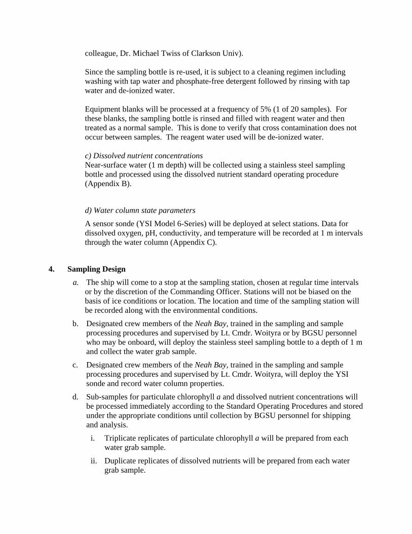
colleague, Dr. Michael Twiss of Clarkson Univ). Since the sampling bottle is re-used, it is subject to a cleaning regimen including washing with tap water and phosphate-free detergent followed by rinsing with tap water and de-ionized water. Equipment blanks will be processed at a frequency of 5% (1 of 20 samples). For these blanks, the sampling bottle is rinsed and filled with reagent water and then treated as a normal sample. This is done to verify that cross contamination does not occur between samples. The reagent water used will be de-ionized water. c) Dissolved nutrient concentrations Near-surface water (1 m depth) will be collected using a stainless steel sampling bottle and processed using the dissolved nutrient standard operating procedure (Appendix B).
d) Water column state parameters
A sensor sonde (YSI Model 6-Series) will be deployed at select stations. Data for dissolved oxygen, pH, conductivity, and temperature will be recorded at 1 m intervals through the water column (Appendix C).
4. Sampling Design a. The ship will come to a stop at the sampling station, chosen at regular time intervals
or by the discretion of the Commanding Officer. Stations will not be biased on the basis of ice conditions or location. The location and time of the sampling station will be recorded along with the environmental conditions.
b. Designated crew members of the Neah Bay, trained in the sampling and sample processing procedures and supervised by Lt. Cmdr. Woityra or by BGSU personnel who may be onboard, will deploy the stainless steel sampling bottle to a depth of 1 m and collect the water grab sample.
c. Designated crew members of the Neah Bay, trained in the sampling and sample processing procedures and supervised by Lt. Cmdr. Woityra, will deploy the YSI sonde and record water column properties.
d. Sub-samples for particulate chlorophyll a and dissolved nutrient concentrations will be processed immediately according to the Standard Operating Procedures and stored under the appropriate conditions until collection by BGSU personnel for shipping and analysis.
i. Triplicate replicates of particulate chlorophyll a will be prepared from each water grab sample.
ii. Duplicate replicates of dissolved nutrients will be prepared from each water grab sample.
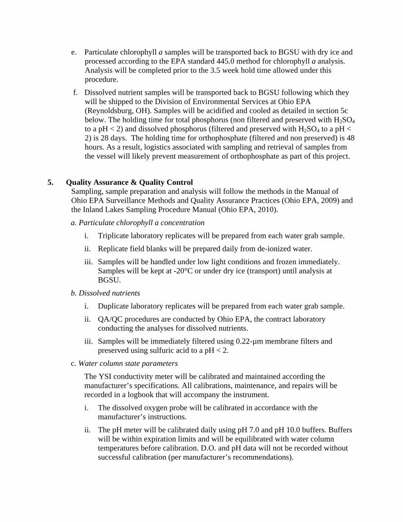
e. Particulate chlorophyll a samples will be transported back to BGSU with dry ice and processed according to the EPA standard 445.0 method for chlorophyll a analysis. Analysis will be completed prior to the 3.5 week hold time allowed under this procedure.
f. Dissolved nutrient samples will be transported back to BGSU following which they will be shipped to the Division of Environmental Services at Ohio EPA (Reynoldsburg, OH). Samples will be acidified and cooled as detailed in section 5c below. The holding time for total phosphorus (non filtered and preserved with H2SO4 to a pH < 2) and dissolved phosphorus (filtered and preserved with H2SO4 to a pH < 2) is 28 days. The holding time for orthophosphate (filtered and non preserved) is 48 hours. As a result, logistics associated with sampling and retrieval of samples from the vessel will likely prevent measurement of orthophosphate as part of this project.
5. Quality Assurance & Quality Control Sampling, sample preparation and analysis will follow the methods in the Manual of Ohio EPA Surveillance Methods and Quality Assurance Practices (Ohio EPA, 2009) and the Inland Lakes Sampling Procedure Manual (Ohio EPA, 2010).
a. Particulate chlorophyll a concentration
i. Triplicate laboratory replicates will be prepared from each water grab sample.
ii. Replicate field blanks will be prepared daily from de-ionized water.
iii. Samples will be handled under low light conditions and frozen immediately. Samples will be kept at -20°C or under dry ice (transport) until analysis at BGSU.
b. Dissolved nutrients
i. Duplicate laboratory replicates will be prepared from each water grab sample.
ii. QA/QC procedures are conducted by Ohio EPA, the contract laboratory conducting the analyses for dissolved nutrients.
iii. Samples will be immediately filtered using 0.22-µm membrane filters and preserved using sulfuric acid to a pH < 2.
c. Water column state parameters
The YSI conductivity meter will be calibrated and maintained according the manufacturer’s specifications. All calibrations, maintenance, and repairs will be recorded in a logbook that will accompany the instrument.
i. The dissolved oxygen probe will be calibrated in accordance with the manufacturer’s instructions.
ii. The pH meter will be calibrated daily using pH 7.0 and pH 10.0 buffers. Buffers will be within expiration limits and will be equilibrated with water column temperatures before calibration. D.O. and pH data will not be recorded without successful calibration (per manufacturer’s recommendations).
6. Credible Data Collection Supervisory and analytical personnel (Dr. McKay, Lt. Cmdr. Woityra, DR. Bullerjahn, Dr. Beall & Ben Oyserman) submitted credentials for consideration to be certified Level 3 Credible Data Personnel and were approved by Ohio EPA in fall 2010. A training session led by Dr. McKay and Lt. Cmdr. Woityra was held on 3 November and again on 6 December for the USCG servicemen to establish sample collection methods and quality criteria. Dan Glomski (Ohio EPA) oversaw the December training session to ensure the crewmembers of the Neah Bay meet Credible Data Collection requirements. USCG servicemen, under the direct supervision of at least one Level 3 certified person, will conduct all sample collection. Monthly (or more frequent) meetings on board the Neah Bay between the project manager (Dr. McKay), Lt. Cmdr. Woityra, and analytical personnel from BGSU, will serve to monitor sampling techniques, discuss data quality performance, and ensure the sampling efforts by the USCG meet the requirements of the study plan and standard operating procedures.
7. Project Deliverables to the Ohio Credible Data Program
This project will provide synoptic data on the concentration of chlorophyll a, dissolved nutrients concentrations in near-surface waters, as well as dissolved oxygen concentrations, conductivity, temperature, and pH of the water column, at stations throughout Lake Erie during the winter season.
8. Qualified Personnel Project Manager Level 3 Certification: Chemical Water Quality Assessment Effective: 11/15/2010 QDC # 00519
Dr. Robert Michael L. McKay
Department of Biological Sciences Bowling Green State University Bowling Green, OH, 43403 Phone: (419) 372-6873 Email: [email protected]
Sampling Supervisor Level 3 Certification: Chemical Water Quality Assessment Effective: 12/22/2010 QDC # 00551
Lt. Cmdr. William Woityra USCGC NEAH BAY (WTGB 105) 1055 E 9th Street Cleveland, OH USA
BGSU Personnel (Level 3 Certified)
Dr. George S. Bullerjahn
Department of Biological Sciences Bowling Green State University Bowling Green, OH, 43403 Phone: (419) 372-8527 Email: [email protected]
Level 3 Certification: Chemical Water Quality Assessment Effective: 11/15/2010 QDC # 00517
Dr. Benjamin F. N. Beall
Department of Biological Sciences Bowling Green State University Bowling Green, OH, 43403 Phone: (419) 372-4209 Email: [email protected]
Level 3 Certification: Chemical Water Quality Assessment Effective: 11/15/2010 QDC # 00518
Mr. Ben Oyserman
Department of Biological Sciences Bowling Green State University Bowling Green, OH, 43403 Phone: (419) 372-6873 Email: [email protected]
Level 3 Certification: Chemical Water Quality Assessment Effective: 11/15/2010 QDC # 00520
Sampling will be conducted by USCG personnel on the Neah Bay under the direct supervision of Lt. Cmdr. Woityra or one of the BGSU Level 3-certified scientists. A training session was conducted by McKay and Oyserman on Nov. 3. A second session was conducted on Dec. 6, 2010. Agency Advisor Dan Glomski attended the training on Dec. 6 and offered advice where necessary.
Sample analysis, data processing, and data analysis will be conducted at BGSU by Drs. McKay, Bullerjahn and Beall, & Mr. Oyserman.
The following crew members of CGC Neah Bay have been trained in sample collection and
processing and will be involved in collection of credible data under the direct supervision of a QDC:
Nicholas Bonner Terrell Douglas Robert Gilmore Andrew Jantzen John Leary Manfred Lee David Moellenbeck Benjamin Peavey Jake Redden David Shaw Timothy Stem Brock Taylor Matthew Tremblay
9. Contract Laboratory Chemical analysis for dissolved nutrient concentrations will be conducted by the Division of Environmental Services, Ohio EPA.
Contact:
Roman Khidekel, Manager Division of Environmental Services Ohio EPA 8955 E Main Street, BLDG 22 Reynoldsburg, OH 43068-3342 Tel: (614)644-4234 Email: [email protected]
10. Statement The persons conducting data collection have not been convicted of or have pleaded guilty to a violation of section 2911.21 of the Revised Code (criminal trespass) or a substantially similar municipal ordinance within the previous five years.
Appendix A Standard Operating Procedure for Chlorophyll-a Sampling Method: Field Procedure for Use by U.S. Coast Guard 1.0 Scope and Application This method is used to filter chlorophyll-a samples from the Great Lakes and Tributary streams. 2.0 Summary of Method A grab lake water sample is collected from a stainless steel sampling bottle at various depths and filtered by vacuum filtration in dim light. The filter is then placed in a screw cap polyethylene culture tube in the dark. The tube is stored in the dark at sub-freezing temperatures and transported to the BGSU laboratory for extraction and analysis. The BGSU laboratory will follow protocol LG405, developed by the EPA’s Great Lakes National Program Office (GLNPO) for water quality surveys of the Great Lakes (appended). 3.0 Apparatus Plastic filter funnel, Pall Filtron (250 mL capacity) Vacuum manifold system to accommodate 3 filter funnels Vacuum system (3-4 psi) GF/F filters, Whatman (25 mm) Screw cap polyethylene tubes Graduated polystyrene pipettes (25 mL; disposable) Pasteur short disposable pipets Rubber bulb Plastic wash bottle, 500 mL Plastic wash bottle, 500 mL, for MgCO3 Filter forceps Opaque sample bottles, 1000 mL (Nalgene or equivalent) 4.0 Reagents Saturated Magnesium Carbonate Solution Add 10 grams magnesium carbonate to 1000 mL of deionized water. The solution is settled for a minimum of 48 hours. Decant the clear solution into a new container for subsequent use. Only the clear "powder free" solution is used during subsequent steps. 5.0 Sample Handling and Preservation Sample collection and preservation will follow the procedures described in the Manual of Ohio EPA Surveillance Methods and Quality Assurance Practices (Ohio EPA, 2009) and the Inland Lakes Sampling Procedure Manual (Ohio EPA, 2010). The entire procedure should be carried out as much as is possible in subdued light to prevent photodecomposition. The frozen samples should also be protected from light during storage for the same reason. During the filtration process, the samples are treated with MgCO3 solution (section 4) to eliminate acid induced transformation of chlorophyll to its degradation product, pheophytin. Samples are stored by station in aluminum foil and transported to the BGSU laboratory in a cooler with dry ice. Analysis should be performed as soon as possible following sampling. 6.0 Field Procedure 6.1 Following sample collection with the stainless steel sampling bottle, samples are transferred to 1000 mL opaque Nalgene bottles, labeled with the station, sample depth, eg. Surface, representing a surface sample 6.2 Place filters, using forceps, textured side up. Assemble the filtration apparatus just prior to filtration. 6.3 Due to differing trophic levels among the Great Lakes, the volume of water filtered varies. For
Lake Erie, 25 mLs of sample are filtered. After inverting the sample bottle several times to create a uniform mixture, carefully draw 25 mL into a pipette and distribute contents into filtration funnel. 6.4 Turn vacuum pressure on, not exceeding 3 psi. Our plans call for use of a hand pump. Check Frequently During Filtration to Insure Pressure Does Not Go Above 3 PSI!!! 6.5 When approximately 10 mL of sample remains on the filter, add 10 drops of the MgCO3 (section 4.1) solution using a disposable pipet. Thoroughly rinse the filter apparatus and graduated cylinder, using a squirt bottle, with deionized water. Turn off vacuum pressure as soon as the liquid disappears to prevent the breakage of cells. 6.6 Using the forceps, fold and remove the filter and carefully place it into the bottom portion of the prelabeled culture tube (see section 10) and close tightly. Lay all tubes flat and completely wrap in aluminum foil. Clearly label the Lake, station and date on masking tape and attach to above mentioned aluminum foil package. Immediately freeze. All the above procedures should be completed in subdued light. 7.0 Quality Control 7.1 Each of the following audits is collected once per lake transect. 7.2 Field duplicates are taken from a second stainless steel sampling bottle collected at about the same time and location as the regular field sample. It is transported from the Niskin bottle to the onboard biology laboratory in an opaque bottle marked as duplicate sample. 7.3 Laboratory duplicates are filtered from the same opaque sample bottle as their corresponding regular field samples. 7.4 Field blanks, consisting of reagent water are carried by an opaque sample bottle from the onboard reagent water supply to the filtration apparatus. The bottle is used only for field blanks and is permanently marked as such. 8.0 Waste Disposal Follow all laboratory waste disposal guidelines regarding the disposal of MgCO3 solutions. 9.0 Shipping Once a transect has been completed or a batch of 35 samples has been completed, wrap all samples into one complete batch and clearly label with date. Pack tightly in a medium sized cooler and fill all spaces with enough dry ice to last 24 hours. Dry ice is considered a hazardous chemical by most shipping companies and has to be accompanied by authorizing paperwork. Once transported to BGSU, the samples should be immediately placed in the freezer. 10.0 Labeling Sample identification information is provided on printed labels both prior to and during the survey. The labels are affixed to the side of the 16 × 100 mm chlorophyll tube. The sample identification number is covered with clear tape in case the tube becomes wet.
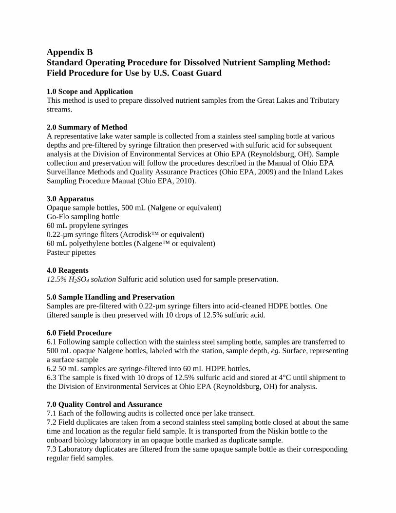
Appendix B Standard Operating Procedure for Dissolved Nutrient Sampling Method: Field Procedure for Use by U.S. Coast Guard 1.0 Scope and Application This method is used to prepare dissolved nutrient samples from the Great Lakes and Tributary streams. 2.0 Summary of Method A representative lake water sample is collected from a stainless steel sampling bottle at various depths and pre-filtered by syringe filtration then preserved with sulfuric acid for subsequent analysis at the Division of Environmental Services at Ohio EPA (Reynoldsburg, OH). Sample collection and preservation will follow the procedures described in the Manual of Ohio EPA Surveillance Methods and Quality Assurance Practices (Ohio EPA, 2009) and the Inland Lakes Sampling Procedure Manual (Ohio EPA, 2010). 3.0 Apparatus Opaque sample bottles, 500 mL (Nalgene or equivalent) Go-Flo sampling bottle 60 mL propylene syringes 0.22-µm syringe filters (Acrodisk™ or equivalent) 60 mL polyethylene bottles (Nalgene™ or equivalent) Pasteur pipettes 4.0 Reagents 12.5% H2SO4 solution Sulfuric acid solution used for sample preservation. 5.0 Sample Handling and Preservation Samples are pre-filtered with 0.22-µm syringe filters into acid-cleaned HDPE bottles. One filtered sample is then preserved with 10 drops of 12.5% sulfuric acid. 6.0 Field Procedure 6.1 Following sample collection with the stainless steel sampling bottle, samples are transferred to 500 mL opaque Nalgene bottles, labeled with the station, sample depth, eg. Surface, representing a surface sample 6.2 50 mL samples are syringe-filtered into 60 mL HDPE bottles. 6.3 The sample is fixed with 10 drops of 12.5% sulfuric acid and stored at 4°C until shipment to the Division of Environmental Services at Ohio EPA (Reynoldsburg, OH) for analysis. 7.0 Quality Control and Assurance 7.1 Each of the following audits is collected once per lake transect. 7.2 Field duplicates are taken from a second stainless steel sampling bottle closed at about the same time and location as the regular field sample. It is transported from the Niskin bottle to the onboard biology laboratory in an opaque bottle marked as duplicate sample. 7.3 Laboratory duplicates are filtered from the same opaque sample bottle as their corresponding regular field samples.
7.4 Field blanks, consisting of reagent water are carried by an opaque sample bottle from the onboard reagent water supply to the filtration apparatus. The bottle is used only for field blanks and is permanently marked as such. 8.0 Waste Disposal Follow all laboratory waste disposal guidelines regarding the disposal of H2SO4 solutions. 9.0 Shipping Once a transect has been completed or a batch of 15 samples has been completed, bottles will be loaded into bags and clearly label with the date. Samples will be stored at 4°C until loaded into a cooler with blue ice for transport to NCWQR. 10.0 Labeling Sample identification information is provided on printed labels both prior to and during the survey. The labels are affixed to the side of the 60 mL sample bottle. The sample identification number is covered with clear tape in case the tube becomes wet.
Appendix C
Standard Operating Procedure for Calibration and Field Measurement Procedures for the YSI Model 6-Series Sondes and Data Logger (Including: Temperature. pH, Specific Conductance, Turbidity and Dissolved Oxygen): Field Procedure for Use by U.S. Coast Guard
1.0 Scope and Application The purpose of this standard operating procedure (SOP) is to provide a framework for calibrating sondes used to measure water quality parameters for surface water from the Great Lakes and Tributary streams. Water quality parameters include temperature, pH, dissolved oxygen, conductivity/specific conductance and turbidity.
This SOP is written specifically for the YSI model 6-Series Sondes (which include the 600R, 600XL, 600XLM, 6820, 6920 and 6600 models), the YSI 650 MDS (Multi parameter Display System) display/logger, and YSI EcoWatch software. The general calibration processes discussed herein are applicable to other manufactures sondes and displays/loggers. Consult the manufacture's instruction manuals for specific procedures.
2.0 Summary of Method This document describes a process for calibrating and performing water quality field measurements using YSI 6-Series Sondes.
3.0 Apparatus
• NIST traceable thermometer (only needed once per year)
• pH Standards of 4, 7, and 10
• Conductivity standards (concentration dependent upon expected field conditions)
• Turbidity standards (concentration dependent upon expected field conditions)
• Deionized and tap water
• Calibration cups
• YSI Sonde with attached pH/ORP, Conductivity, Dissolved Oxygen, and Turbidity probes
• YSI 650 MDS Multiparameter Display System (display logger)
• Sonde communications cable
• Zobell Solution
• Batteries
4.0 Calibration Check the display/logger to determine the battery level in the display/logger to see if recharging or new batteries are necessary. Prior to calibration, all instrument probes on the sonde must be cleaned according to the manufacturer's instructions. Failure to perform this step can lead to erratic measurements. The probes must also be cleaned by rinsing with deionized water before and after immersing the probe in a calibration solution. For each of the calibration solutions, provide just enough volume so that the probe and the temperature sensor are sufficiently covered. When done with the calibration solutions do not return it to the original bottle, save solution in separate container or dispose of it properly. When using the Sonde for long-term deployment and using the "Autosleep RS232, and Autosleep SDI12" functions, the instrument must be calibrated in these modes. For manual measurements this function should be turned off (see section 5.5.1.3) prior to calibration.
4.1 Temperature
For instrument probes that rely on the temperature sensor (pH, dissolved oxygen/specific conductance, and oxidation-reduction potential), the sonde temperature sensor needs to be checked for accuracy against a thermometer that is traceable to the National Institute of Standards and Technology (NIST). This accuracy check should be performed at least once a year, and the date and results of the check kept on file. Below is the verification procedure.
4.1.1 Once a year, the accuracy of the instrument must be verified by checking the endpoints of the desired temperature range. For example, if the desired temperature range is O °C to 40.0 °C, the instrument must be within the ± 0.15 °C of both end points.
4.1.2 Place a thermometer that is traceable to the NIST into the water and wait for both temperature readings to stabilize.
4.1.3 Compare the two measurements. The instrument's temperature sensor must agree with the reference thermometer within the accuracy of the sensor (± 0.15 °C). If the measurements do not agree, the instrument may not be working correctly and the manufacturer should be contacted.
4.2 pH
The pH of a sample is determined electrometrically using a glass electrode. Choose the appropriate standards that will bracket the expected values at the sampling locations. For this procedure three standards will be used (pH 4, pH 7, & pH 10). If the probe is slow to response refer to the Troubleshooting section.
4.2.1 Rinse probe with deionized water and shake off excess water. Allow the buffered samples to equilibrate to the ambient temperature.
4.2.2 Place the probes (at least pH and temperature probes) on the sonde into the pH 7 buffer.
4.2.3 On the display/logger use the up/down arrow keys to highlight the "Calibrate" option and press the enter key.
4.2.4 Highlight the "pH option and press enter.
4.2.5 Highlight the "3-point" option and press enter.
4.2.6 Input the value of the buffer, which is 7.00 and press enter.
4.2.7 Wait for the value of pH to stabilize and then press enter. Wait for "Calibrated" message. If an "Out of Range" message appears, do not accept, check the probe and refer to operator's manual or Troubleshooting section.
4.2.8 Place the pH probe into a pH 4.00 buffer.
4.2.9 Press enter key to continue calibration
4.2.10 When prompted, enter the pH of the second buffer, "4.00. Wait for "Calibrated" message, and press any key to continue.
4.2.11 Rinse probe with deionized water and shake off excess water
4.2.12 Place the pH probe into a pH 10.00 buffer.
4.2.13 Press enter key to continue calibration
4.2.14 When prompted, enter the pH of the third buffer, "10.00". Wait for "Calibrated" message, and press any key to continue.
4.2.15 Rinse probe with deionized water and shake off excess water.
4.2.16 Exit the calibration menu and go to the "Sonde Run" mode. Insert probe into pH 7 buffer and make sure it is reading correctly (± 0.05). If buffer reading is not correct, repeat the calibration procedure.
4.3 Specific Conductance
Conductivity is used to measure the ability of an aqueous solution to carry and electrical current.
Specific conductance is the conductivity value corrected at 25 °C.
4.3.1 Place the cleaned probes into the specific conductivity standard solution, making sure that the specific conductivity probe is fully submerged. For studies where conductivity is a critical parameter (non-critical parameters will be identified in the QAPP), the accuracy of the instrument must be verified by checking the endpoints of the desired conductivity range to insure linearity. Calibrate with one of the standards (the high standard) and check the instrument with a low standard. At the end of the monitoring period check the instruments with both standards. If you are using a small amount of calibration solution or standards that are easily contaminated first rinse the probe(s) with the conductivity standard. Where conductivity is a non-critical measurement you can check and calibrate the instrument with one calibration solution.
4.3.2 Return to the display/logger main menu and select "Calibrate" and press enter.
4.3.3 Select "Conductivity” and press enter.
4.3.4 Select "SpCond" and press enter.
4.3.5 Enter the standard concentration in mS/cm and press enter. The standard concentration should be just above the highest concentrations you expect to measure.
4.3.6 After the specific conductivity reading has stabilized press enter to calibrate. Wait for the "calibrated" message to appear. If the Sonde should report "Out of Range" do not override the error message, instead recheck the standard and go to the Troubleshooting section for more help.
4.3.7 Exit the calibration menu and go to the "Sonde Run" mode and record the concentration (make sure it is reading within 5% of standard value).
4.3.8 To check the calibration with a second standard (low), rinse probe with deionized water and insert probe in second standard and make sure it is reading within 10%. A second standard is used to check the calibration at the low range and to bracket the expected concentrations. This must be performed when conductivity is a critical measurement.
4.4 Dissolved Oxygen
Dissolved oxygen (DO) content in water is measured using a membrane electrode. The DO probe's membrane and electrolyte solution should be inspected for any damage or air bubbles prior to calibration. If air bubbles or damage are present, replace the membrane according to manufacturer suggestions. (After changing the membrane, for accurate measurements, you must wait 6 - 12 hours before use to allow the membrane to equilibrate) YSI 6-Series DO probe must be calibrated using the calibration cup provided with the sonde or by wrapping the sonde probe guard with a wet towel.
The DO is calibrated in the field prior to taking measurements and the final post calibration (verification) check should also be performed in the field before the instrument is turn off and after all measurements are taken.
When calibrating DO and not using the auto sleep function, the instrument must be turned on (warmed up) for 15 minutes prior to calibration. When calibrating the DO for unattended sampling and using the auto sleep function, the instrument should not be warmed up before calibrating (it should be calibrated when the instrument is cool, since it is cool when the instrument is taking readings).
Calibration of the DO probe requires inputting the current barometric pressure. The YSI 650 Display/logger has a barometer within the unit and automatically provides this during the calibration procedure. Other display/loggers may not supply the barometric pressure, in this case you will need a separate barometer.
Two calibration procedures are listed below for dissolved oxygen, one for sampling applications and one for long-term monitoring applications.
4.4.1 Calibration Procedure for Discrete Sampling (non deployment) Applications
The dissolved oxygen probe is calibrated each day prior to use. An initial inspection and calibration should be performed the day before to assure the
membrane is in good shape the instrument is working properly. Follow the procedure below to calibrate.
4.4.1.1 Clean all of the probes on the sonde with tap (or clean ambient water) water. Shake off excess water.
4.4.1.2 Place approximately 118 inch of water in the bottom of the calibration cup. Place the probe end of the sonde into the cup. Engage only 1 or 2 threads of the calibration cup to insure the DO probe is vented to the atmosphere. [An equivalent alternative method is to wrap the probe guard (which is attached to the sonde) with a wet towel and place the sonde in a 5 gallon bucket with 1 inch of water in it.]
Make sure that the DO and temperature probes are NOT immersed in water and that the Sonde cup is not in direct sunlight. Wait approximately 10 minutes for the air in the calibration cup to become water saturated and for the temperature to equilibrate.
4.4.1.3 For manual sampling applications the dissolved oxygen probe is continuously pulsing, therefore the "Autosleep RS232" function should be deactivated. (The "Autosleep SDI12" does not effect the manual sampling and can remain on.) From the "Main" menu on the display/logger, select the "System Setup" option and press enter. Then select the "Advanced" option and press enter. Select the "Autosleep RS232" option and press enter to obtain the "off' setting. Then press the "ESC" button until returning to the main menu.
4.4.1.4 From the calibration menu select the "Dissolved Oxy” option, then the DO% option (Note: For the YSI 6-Series Sondes, calibration of dissolved oxygen by the DO% procedure also results in the calibration of the DO mg/l mode and vice versa.)
4.4.1.5 Enter the current barometric pressure in mm of Hg. The correct pressure will automatically apex, double check this value with the reading provided in the lower right hand corner of the display.
4.4.1.6 Press enter and then wait for the DO% reading to equilibrate. Press enter to accept the calibration. Press enter again to return to the calibration menu.
4.4.1.7 Immediately enter the "Sonde Run" mode and record the temperature, dissolved oxygen in mg/l and %, and the barometric pressure used for calibrating. The DO should be within ± 0.2 of saturation value. If not, go to section 4.5.1.4 to recalibrate.
4.4.1.8 For critical DO (non-critical parameters will be identified in the QAPP) applications, verify the probe with a zero DO solution.
1) Place the probe in a zero DO solution.
2) Verify the probe reads < 0.5mgfl (or to the range specified in QAPP)
3) Rinse probe and store the probe in tap water.
4.4.1.9 Fill the calibration cup half way with tap water and screw on to the sonde. The sonde is now ready for use.
5.0 Troubleshooting 5.1 Occasionally problems are encountered during a calibration and the instrument must be uncalibrated to return the instrument to factory settings. Uncalibration can be performed following these steps.
5.1.1 Access the desired parameter to uncalibrate in the calibrate menu.
5.1.2 When prompted to input a number for a standard, hold the enter key down and press the "esc" key. Highlight the "yes" key and press enter. (Please note: This procedure is the equivalent of entering the command "uncal" from the YSI 610 logger at the numeric calibration prompt.)
5.2 pH
5.2.1 Refer to the Sonde Performance Worksheet. If a probe is slow to respond, recondition the probe according to the "Sonde Care and Maintenance Section" of the users manual.
5.2.2 To check the condition of the probe record the millivolts for each buffer. The millivolt output is the unprocessed pH output, the acceptable tolerance for each buffer is shown below:
Buffer 4 = +180 ± 50 mv
Buffer 7 = 0 ± 50 mv
Buffer 10 = -180 ± 50 mv
When the probe is new, the ideal number are close to 0 and 180, then as the probe begins to age, the numbers will move and shift to the higher side of the tolerance.
5.2.3 After recording the pH millivolts for the calibration points determine the slope of the sensor. This is the difference between the two calibration points. For example, if we recorded a + 5 mv for buffer 7 and a -175 for buffer 10, the slope would be 180. The acceptable range for the slope is 165 to 180. Once the slope drops below 165, the sensor should be replaced.
5.3 Conductivity
5.3.1 Refer to the Sonde Performance Worksheet
5.3.2 When the calibration has been accepted, check the conductivity cell constant which can be found in the sonde's "Advanced Menu" under "Cal Constants". The acceptance range is 4.55 to 5.45. Numbers outside this range usually indicated a problem in the calibration process or a contaminated standard was used.
5.4 Dissolved Oxygen
5.4.1 Refer to the Sonde Performance Worksheet
5.4.2 Go to the Sondes "Report" menu and enable the "DO Charge". Now go to the "Run" menu and start the sonde in the "Sonde Run" mode. Record the DO Charge after about 5 minutes. The number should be between 25 and 75. If this is not true contact the manufacturer or replace the probe.
5.4.3 When the calibration is complete go to the sonde's "Advanced Menu" and to the "Cal Constants" and record the "DO Gain". The gain should be between 0.7 and 1.4. If this is not true contact the manufacturer or replace the probe.
6.0 Measurements Sondes can be used for either discrete sample measurements or be deployed for a period of time to record measurements. Each of these types of measurements requires different configurations of the sonde memory and display logger.
6.1 Discrete sample measurements
6.1.1 From the main menu select the "Sonde Run" option and press enter.
6.1.2 Place the Sonde into the water to be analysed, and watch the variations in the desired parameters.
6.1.3 After a few minutes or when the variations are less than:
0.1 °C temperature 0.02 su pH 0.02mg/l D.O. 5 uS/cm conductivity 0.5 NTU Turbidity
Log the measurements in the project's log book.
6.1.4 If the measurement is to be logged in the sonde memory, the select the "Log one sample" option from the Sonde Menu, and press enter.
6.1.5 If a series of measurements from one site is to be logged in the sonde memory, select the "Start Logging" option from the Sonde Menu and press enter. After a pre-determined amount of time select the "Stop Logging" option to stop logging measurements.
7.0 Data Management and Records Management All results of calibration must be documented and kept in a project's log book. At a minimum the following should be kept as part of the documentation: the instrument's model number, instrument identification number, standards used to calibrate the instruments, calibration date, the instrument readings, and the analyst.