Creating Hot Streets: Developing an Automated Approach Using ModelBuilder

by

Quincy Tamunotonye-Mieba Tom-Jack

A Thesis Presented to the

Faculty of the USC Graduate School

University of Southern California

In Partial Fulfillment of the

Requirements for the Degree

Master of Science

(Geographic Information Science and Technology)

December 2018

Copyright © 2018 by Quincy Tom-Jack

All rights reserved

iii

Table of Contents

List of Figures ................................................................................................................................ vi

List of Tables ............................................................................................................................... viii

Acknowledgements ......................................................................................................................... x

List of Abbreviations ..................................................................................................................... xi

Abstract ......................................................................................................................................... xii

Chapter 1 Introduction .................................................................................................................... 1

1.1. Motivation ...........................................................................................................................3

1.2. Questions.............................................................................................................................5

1.3. Study Area ..........................................................................................................................6

1.4. Thesis Outline .....................................................................................................................8

Chapter 2 Background .................................................................................................................... 9

2.1. Crime Analysis....................................................................................................................9

2.1.1. Types of Crime Analysis .........................................................................................10

2.1.2. Tactical Crime Analysis and Crime Mapping .........................................................12

2.2. Spatial Statistics for Clustering .........................................................................................17

2.3. Hot Spot Policing ..............................................................................................................18

2.3.1. Advantages of Hot Spot Policing .............................................................................19

2.3.2. Current Development of Hot Streets for Hot Spot Policing ....................................20

Chapter 3 Methodology ................................................................................................................ 21

3.1. Research Design................................................................................................................21

3.2. Data Selection and Sources ...............................................................................................23

3.2.1. Atlanta City Limit ....................................................................................................24

3.2.2. Streets .......................................................................................................................24

3.2.3. Crimes ......................................................................................................................26

iv

3.3. GIS Procedures and Analysis Models...............................................................................29

3.3.1. Select City Streets Excluding Expressways .............................................................29

3.3.2. Select Crime Type and Shift ....................................................................................31

3.3.3. Show Selected Crimes within the City ....................................................................31

3.3.4. Spatial Join ...............................................................................................................31

3.3.5. Project Streets and Calculate Crimes Per Mile (CPM) ............................................32

3.3.6. Generate Spatial Weight Matrix (SWM) File ..........................................................33

3.3.7. Spatial Autocorrelation ............................................................................................37

3.4. Runs and Purpose ..............................................................................................................38

Chapter 4 Results .......................................................................................................................... 40

4.1. Hot Street Model ...............................................................................................................40

4.2. Spatial Autocorrelation .....................................................................................................43

4.3. Hot Street Result ...............................................................................................................43

4.3.1. Part I .........................................................................................................................46

4.3.2. Auto Theft ................................................................................................................49

4.3.3. Day Shift ..................................................................................................................51

4.3.4. Evening Shift ...........................................................................................................53

4.3.5. Morning Shift ...........................................................................................................55

4.3.6. Weekday ..................................................................................................................57

4.3.7. Weekend ..................................................................................................................59

4.3.8. Part I Houston, Texas. ..............................................................................................61

Chapter 5 Discussion and Conclusions ......................................................................................... 63

5.1. Findings and Impact ..........................................................................................................63

5.1.1. Model .......................................................................................................................63

5.1.2. Hot Streets Results ...................................................................................................64

v

5.2. Limitations ........................................................................................................................68

5.3. Future Research and Recommendations ...........................................................................68

5.4. Conclusion ........................................................................................................................69

References ..................................................................................................................................... 70

Appendix A: Detailed Model Screenshots .................................................................................... 74

vi

List of Figures

Figure 1. Map of Atlanta, Georgia .................................................................................................. 7

Figure 2. Gi* statistics formula. Source: Esri 2018 ...................................................................... 18

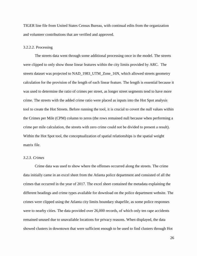
Figure 3. Screenshot of crime locations (left) and the associated street names (right) from a

random sampling across the full dataset ....................................................................................... 28

Figure 4. Flowchart of Hot Street Model ...................................................................................... 30

Figure 5. Screenshot of Spatial Join tool with inputs ................................................................... 32

Figure 6. Screenshots of tools used to generate a near table for the SWM file ............................ 34

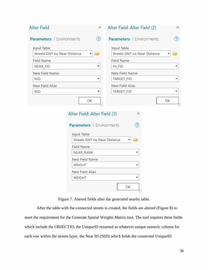
Figure 7. Altered fields after the generated nearby table. ............................................................. 36

Figure 8. Generate Spatial Weights Matrix tool ........................................................................... 37

Figure 9. Hot Spot Analysis tool and parameters ......................................................................... 38

Figure 10. Hot Street Model as Geoprocessing Tool .................................................................... 41

Figure 11. Hot Street Model ......................................................................................................... 42

Figure 12. Hot Street map of Part I crimes ................................................................................... 47

Figure 13. Zoomed in SW section of the Part I Hot Street Map ................................................... 48

Figure 14. Hot Street map of Auto Theft and Vehicle Larceny.................................................... 50

Figure 15. Hot Street map of crimes that occurred during the day shift ....................................... 52

Figure 16. Hot Street map of crimes that occurred during the evening shift ................................ 54

Figure 17. Hot Street map of crimes that occurred during the morning shift ............................... 56

Figure 18. Hot Street map of weekday crimes .............................................................................. 58

Figure 19. Hot Street map of weekend crimes .............................................................................. 60

Figure 20. Part I Hot Street of Central Houston, Texas ................................................................ 62

vii

Figure 21. First four model groups ............................................................................................... 74

Figure 22. Central model groups .................................................................................................. 75

Figure 23. Change Null Values to Zero group .............................................................................. 76

Figure 24. Generate Spatial Weight Matrix group........................................................................ 77

Figure 25. Spatial Statistics group ................................................................................................ 78

viii

List of Tables

Table 1. List of sources, and description of each required data. ................................................... 23

Table 2. Summary of Required Software. .................................................................................... 24

Table 3: List of different runs, crime counts and run times. ......................................................... 39

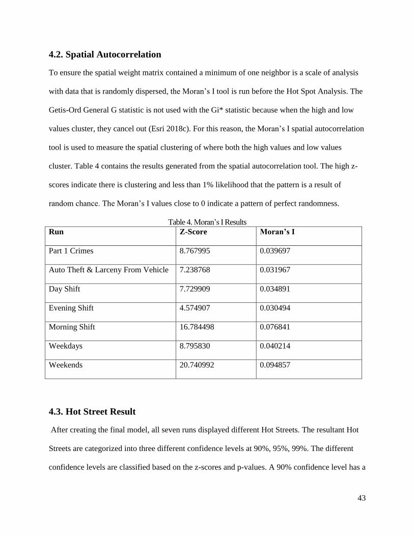
Table 4. Moran’s I Results ............................................................................................................ 43

Table 5. Number of Hot Streets generated from the model. ......................................................... 45

ix

This paper is dedicated to my family and friends who provided me with constant support

throughout my schooling process, and to all the teachers and professor who have trained me to

this point for always believing in me.

x

Acknowledgements

I am grateful to my supervisor, Dr. Laura Loyola, for all the guidance, belief, support,

and motivation provided to me during the thesis development and writing process. I also

appreciate the guidance provided by the other thesis committee members Dr. John Wilson and

Dr. Yao-Yi Chiang. I am thankful to my parents Sir Engr Erefaa and Queen Tom-Jack, my

siblings, and God for providing the opportunity to attend this institution. I would also like to

thank the tactical crime analysts Glenn Grana and Robert Petersen who shared some of the

information needed to develop this thesis. With a special mention to some of my graduate and

undergraduate professors Dr. Jennifer Swift, Dr. Jacque Kelly, Dr. Fredrick Rich, Dr Kelly

Vance, Dr. James Reichard, Dr. Charles H. Trupe, It was terrific to have the opportunity to

attend your classes, and perform some research alongside which solidified my experience and

confidence to perform this research.

xi

List of Abbreviations

ARC Atlanta Regional Commission

CL Confidence Level

CPM Crimes Per Mile

CPTED Crime prevention through environmental design

GIS Geographic information system

GISci Geographic information science

GIST Geographic Information Sciences & Technology

HSA Hot Street Analysis

IACA International Association of Crime Analysts

LEA Law Enforcement Agencies

MAUP Modifiable Areal Unit Problem

NYPD New York Police Department

OSM Open Street Map

PCS Projected Coordinate System

USGS United States Geological Survey

USC University of Southern California

xii

Abstract

The creation of Hot Streets can positively influence the crime reduction efforts by law

enforcement agencies (LEAs) by decreasing patrolled Hot Spot areas and more directly focusing

efforts at the street level. As there has been no easy way of determining Hot Streets, police

officers patrol general areas that vary in size and difficulty of patrol. The purpose of this study is

to create a model within a GIS, particularly ArcGIS Pro, for all users who wish to accurately and

efficiently analyze crime patterns on a street level. The model shows all users, especially the

LEA tactical analysis department, a simple but effective means of using a GIS to improve current

spatial crime analysis methods by the addition of Hot Streets. This study demonstrates how to

analyze and automate the creation of Hot Streets within the ModelBuilder pane for the city of

Atlanta, Georgia. The research provides users with places for the acquisition of GIS data,

methods and input parameters required for processing data prior to incorporation in the model as

well as within the model, and the proper sequence of tool utilization for analysis within the

model. This process resulted in Hot Street maps with several streets classified based on the crime

cluster confidence levels of 90% and above for the city of Atlanta. The Hot Street provides

results for seven confidence levels; which include high and low value crime clusters at 90%,

95%, and 99% respectively, and a final group of streets without a significant cluster. The

developed model was found to be an excellent tool in analyzing crime patterns on a street level

and creating the Hot Street maps at different scales. Both LEAs and civilians can utilize the

developed Hot Street implementation, as it provides a way to reduce crimes through hot street

policing and crime prevention through environmental design.

1

Chapter 1 Introduction

Crime, like any other event, always occurs at a particular place and time. Geographic

Information Systems (GIS) have been used by Law Enforcement Agencies (LEAs) to help their

crime analysis divisions visually represent and understand crime patterns over space and time.

Based on a variety of crime theories, there are several methods one can employ for crime

analysis which aid in crime reduction efforts by LEAs, especially within high crime areas.

Geospatial crime analysts currently use spatial analysis and statistic tools to perform crime

analysis and determine the high crime areas. Authors on the subject have mainly concentrated on

mapping crime point density, kennel density, hot spot, Hot Spot, and heat maps; while finding

correlations with the help of R and R-ArcGIS Bridge, or other statistical software integrated with

ArcGIS (e.g., Scott and Warmerdam 2017; Trepanier 2014; Bruce and Smith 2011; Boba 2005).

One of the most popular methods of the listed techniques is Hot Spot (upper case) analysis,

which are areas that suffer from statistically significant clusters of crime. As a few streets contain

the majority of crime in negatively affected neighborhoods, most studies conclude that patrols of

Hot Spots in those neighborhoods and the remainder of the city have resulted in reductions in

crime (Braga et al. 2012; Schnell et al. 2016). Although the current methods fulfill their goal of

visually representing crime occurrences and helping LEAs and civilians be aware of what is

happening around them, they are lacking in a more accurate representation when studying crimes

on the street level.

Currently, police officers patrol general areas, as there has been no easy way of

delineating linear hot spots also known as hot streets (Eck et al. 2005). Hot Streets are resultant

crime clusters analyzed with statistical proximity relationships at the street level. In this

document, a hot spot/ hot street (lower case) refers to the general term of identified crime

2

clusters with no spatial statistical backing, while a Hot Spot/ Hot Street (upper case) is a result of

spatial statistical output. Based on the reviewed literature there is only one methodology that has

been published on developing Hot Streets with the same Getis Ord Gi* statistic used for Hot

Spot analysis (Brazil et al., 2017). One problem with the spatial analysis in the published

methodology is that it uses Euclidean distance rather than the actual road network to assess Hot

and Cold Streets. Different crime areas separated by a river or a major highway might be close

together as the crow flies (Euclidean distance), but far away from each other on a road network

with few bridges or underpasses (Esri, 2018b). Since the Hot Spot analysis tool is looking for

high crime rates that cluster close together, accurate connectivity is essential. None of the

reviewed papers for determining a Hot Street account for the adjacent street crime values, the

same way the area Hot Spot analysis takes account of nearby connected crime clustered areas

when selected. This information is essential because crime concentrates at a micro-scale /

minimal units of geography (Weisburd et al. 2012; Weisburd et al. 2015), and with changing

policing patterns, crime is not stagnant and can migrate to nearby regions. Hot Streets can

provide the missing high level of precision for observing crime patterns on each street. As seen

in several examples (e.g., Eck et al., 2005; Trepanier, 2017), most of the current street analyses

of crime patterns include the use of total crime count by street symbolized with graduated

symbols, graduated colors, and point density raster attachment, but none of these methods

provide statistical relationships between connected roads. Thus, the current methods do not meet

the definition of Hot Streets within this document and the needs to have Hot Street analysis

available.

This study demonstrates an effective way of depicting Hot Streets within the city of

Atlanta, Georgia with the use of a GIS. The primary research goal is to add to the current

3

literature on crime analysis that utilizes a GIS by applying the use of the Getis-Ord Gi* statistic,

used in the generation of Hot Spot areas, to developing Hot Streets. The Getis-Ord Gi* statistic

delineates statistically significant spatial clusters once the crimes are attached to the nearest

streets. This research will present an automated model for the achievement of the set goal,

enabling people of all experiences and levels to perform the analysis. Within the police

department this analysis will be performed by tactical crime analysts who may or may not have a

geospatial degree. Both LEAs and civilians with basic GIS knowledge can efficiently utilize the

Hot Streets methodology developed from this research; the results of which will provide an

effective way to reduce crimes through whatever recommendations are provided by the

administrative crime analysis department. Example of recommendations include Hot Street

policing, and increased civilian safety by keeping them away from or making them aware of

dangerous streets during their commutes. The end test result for a successful model is an overlay

of the identified Hot Streets and a currently used high crime detection method such as the kernel

density, in order to see the similarity between results from a point area analysis to a linear street

analysis of crime distribution and also any increase in specificity.

1.1. Motivation

The enhancement of the Hot Street Analysis (HSA) and use of the HSA within a GIS is

the principal goal of this research. The motivation behind this is to assist tactical analysis teams

with a more in-depth and geographically localized result. To achieve the goal (or aim), spatial

statistics that account for street connectivity are added to current Hot Street procedures. The Hot

Streets not only allow more direct and safer navigation through or away from Hot Spots, but the

enhancement of Hot Streets also provides precise patrol route possibilities for LEAs. These

4

enhanced patrol routes can result in improved crime reduction efforts, and in return keep the

civilians within the city safer.

GIS tools can help to improve navigation within or past Hot Spots through the creation of

Hot Streets. Currently, only Hot Spots are developed within ArcGIS with the use of Getis-Ord

Gi* (Esri 2018). Hot Spot policing has resulted in noteworthy crime reduction through police

concentration in smaller crime areas (Braga et al. 2012; Grana and Windell 2016), and policing

these Hot Spot areas is mostly done with vehicles. However, this form of analysis is not helpful

for navigational purposes because no work to date has reclassified Hot Spot data to the streets

within the Hot Spot areas. There is a need to be able to replicate the creation of Hot Spots to a

street level as Hot Streets that both the police and civilians travel on. The resulting method

would result in safer travels for civilians, more precise street segments within regions for patrol,

reduced crime along the streets within those Hot Spot areas, and a replicable method for all

crime analysis departments for Hot Street Policing. Civilians would have a more positive

commuting experience because of this research, as they will be more spatially aware of the

potential threats along their routes.

This work contributes to studies on the creation of hot streets. Hot street creation often

happens on a neighborhood level, as it is used to direct patrol routes in dangerous neighborhoods

(Gwinn et al. 2008). The Hot Streets created in this work can be used on multiple levels to

examine street-level relationships of crime through high and low clusters via Z-scores and P-

values that help display spatial clusters of high and low crime streets.

This study will attempt to create a standardized model that all police departments and

civilians in different cities can adopt. Though various issues, such as how many nearby streets

should influence a single linear segment calculation, may result in slight changes to the

5

developed Hot Street Model in different regions. This model will help simplify the process of

identifying Hot Streets so that any user can apply this crime analysis for tactical purposes. The

research will also aid police and civilians to import data into a GIS and to process the data into

meaningful information. Finally, it builds the capacity of police departments to use GIS as a tool

to serve their civilian population. The model tool can serve the population through the generation

of specific street names with crime clusters which provide the chance for residents to take

personal action in increasing personal safety via home fencing, surveillance, etc.

1.2. Questions

Developing a Hot Street Analysis (HSA) model to aid current studies and applications of

crime and street relationships comes with its own set of questions and considerations. These

include the modifiable areal unit problem (MAUP), tool availability, design and effectiveness,

and replicability.

The MAUP occurs because different aggregation schemes yield different results despite

using the same analysis and data. Despite this problem, the different results are often valid as

different analyses seek to answer different questions on a variety of scales (Esri 2018a).

According to Brazil et al. (2017) because smaller units (streets) are more homogeneous, they can

be better measures of environmental characteristics. This means that the results which are valid

for the street level crime study may be more accurate than broader area aggregation techniques.

There are several tools developed within a GIS for specific purposes. Within a

ModelBuilder pane in ArcGIS Pro, these tools can be combined to accomplish significant tasks

requiring the acquisition of tools. Hot Street creation is an example of one of the tasks that

requires multiple tools to work within ModelBuilder, and fortunately, the needed tools and add-

ins are all available with the appropriate extensions in Esri’s ArcGIS platforms.

6

Designing the model also requires a process of measuring the full effectiveness of each

individual tool selected and the proper order in which these tools are utilized. Within the

ModelBuilder there will need to be decisions made on whether the individual tools achieve the

desired outcome and where the tool can be improved, either through setting different parameters

or the addition of subsequent tools. The intention of building this model is to replicate this

process so that it can enhance Hot Street Analysis.

As a result, the question of replicability comes up. With slightly different data inputs,

care will have to be taken to ensure anyone in any city can pick and use the model on the fly.

This research will determine if the developed model can be used to accomplish all the listed

goals within a study area different from that in this research through making sure that all the

input model parameters can be used for any study area and testing on an additional (secondary)

dataset.

1.3. Study Area

This research will develop its model with data from the city of Atlanta, Georgia because

of the author’s proximity to the police department, current contacts with the Tactical Crime

Analysis Unit, and familiarity with the environment. The city of Atlanta (Figure 1) is the capital

of the state of Georgia and is situated within two different counties: Fulton and Dekalb counties.

The city covers 133.9 square miles of which only 0.63 percent is covered by water. Atlanta is

currently the ninth largest metropolitan area in the US with over 5.7 million people, and

currently has over 2,000 sworn police officers, making Atlanta’s Police Department the largest

law enforcement agency in the state of Georgia (City of Atlanta, 2018). The city is home to a

diverse population, with varying income levels throughout the city.

7

Figure 1. Map of Atlanta, Georgia

8

1.4. Thesis Outline

The remainder of this thesis begins with a literature review, followed by the presentation

of the methodology used to develop the model within ModelBuilder, the results, a discussion of

findings and comparisons to other crime analysis, and a conclusion.

Chapter 2, reviews related literature on current cluster analyses and uses. The current

methods of Hot Spot analysis will be explained in detail since this informed the choice of

methods for the generation of crime Hot Streets. Literature supporting the development of the

model is introduced, as well as a brief explanation of the statistics.

In Chapter 3, the developed methods used in creating Hot Streets are discussed. The

chapter presents the model for the HSA with the supporting documentation for the use of each

tool. The chapter also lists required data inputs and the best sources to yield needed results.

Chapter 4 presents the final HSA model and results of the multiple and varied model

runs. The resulting street layer should display the statistically significant crime clusters by street.

These results are presented with kernel density outputs as well to verify and compare Hot Street

crime clusters to a traditional method of crime visualization.

Chapter 5 interprets the significance of the results, and how they compare to other crime

analyses currently performed. The chapter explains in detail how the results fulfill the goals of

the project, provides additional insights into the model, as well as possible adjustments that could

affect the results. This chapter also provides conclusions based on the importance of this research

and the ability of crime analysts and police to determine Hot Streets.

9

Chapter 2 Background

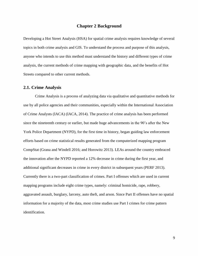
Developing a Hot Street Analysis (HSA) for spatial crime analysis requires knowledge of several

topics in both crime analysis and GIS. To understand the process and purpose of this analysis,

anyone who intends to use this method must understand the history and different types of crime

analysis, the current methods of crime mapping with geographic data, and the benefits of Hot

Streets compared to other current methods.

2.1. Crime Analysis

Crime Analysis is a process of analyzing data via qualitative and quantitative methods for

use by all police agencies and their communities, especially within the International Association

of Crime Analysts (IACA) (IACA, 2014). The practice of crime analysis has been performed

since the nineteenth century or earlier, but made huge advancements in the 90’s after the New

York Police Department (NYPD), for the first time in history, began guiding law enforcement

efforts based on crime statistical results generated from the computerized mapping program

CompStat (Grana and Windell 2016; and Horowitz 2013). LEAs around the country embraced

the innovation after the NYPD reported a 12% decrease in crime during the first year, and

additional significant decreases in crime in every district in subsequent years (PERF 2013).

Currently there is a two-part classification of crimes. Part I offenses which are used in current

mapping programs include eight crime types, namely: criminal homicide, rape, robbery,

aggravated assault, burglary, larceny, auto theft, and arson. Since Part II offenses have no spatial

information for a majority of the data, most crime studies use Part I crimes for crime pattern

identification.

10

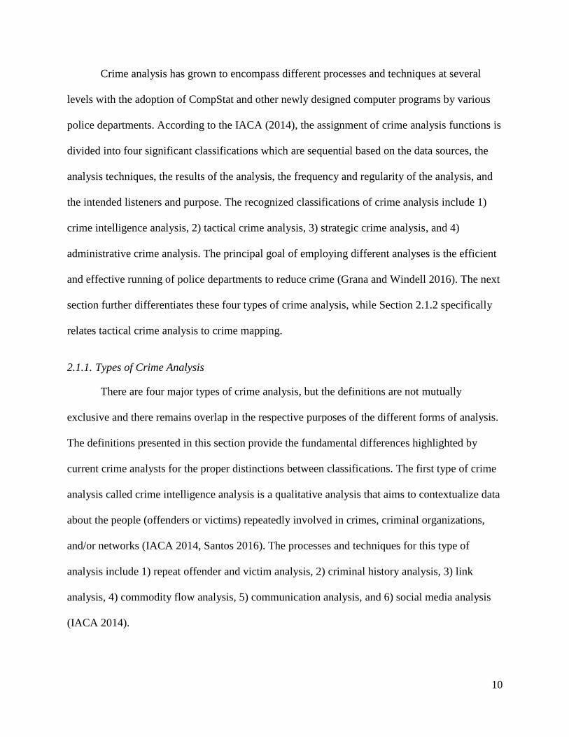
Crime analysis has grown to encompass different processes and techniques at several

levels with the adoption of CompStat and other newly designed computer programs by various

police departments. According to the IACA (2014), the assignment of crime analysis functions is

divided into four significant classifications which are sequential based on the data sources, the

analysis techniques, the results of the analysis, the frequency and regularity of the analysis, and

the intended listeners and purpose. The recognized classifications of crime analysis include 1)

crime intelligence analysis, 2) tactical crime analysis, 3) strategic crime analysis, and 4)

administrative crime analysis. The principal goal of employing different analyses is the efficient

and effective running of police departments to reduce crime (Grana and Windell 2016). The next

section further differentiates these four types of crime analysis, while Section 2.1.2 specifically

relates tactical crime analysis to crime mapping.

2.1.1. Types of Crime Analysis

There are four major types of crime analysis, but the definitions are not mutually

exclusive and there remains overlap in the respective purposes of the different forms of analysis.

The definitions presented in this section provide the fundamental differences highlighted by

current crime analysts for the proper distinctions between classifications. The first type of crime

analysis called crime intelligence analysis is a qualitative analysis that aims to contextualize data

about the people (offenders or victims) repeatedly involved in crimes, criminal organizations,

and/or networks (IACA 2014, Santos 2016). The processes and techniques for this type of

analysis include 1) repeat offender and victim analysis, 2) criminal history analysis, 3) link

analysis, 4) commodity flow analysis, 5) communication analysis, and 6) social media analysis

(IACA 2014).

11

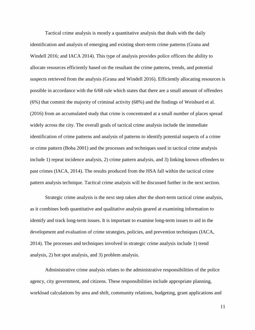
Tactical crime analysis is mostly a quantitative analysis that deals with the daily

identification and analysis of emerging and existing short-term crime patterns (Grana and

Windell 2016; and IACA 2014). This type of analysis provides police officers the ability to

allocate resources efficiently based on the resultant the crime patterns, trends, and potential

suspects retrieved from the analysis (Grana and Windell 2016). Efficiently allocating resources is

possible in accordance with the 6/68 rule which states that there are a small amount of offenders

(6%) that commit the majority of criminal activity (68%) and the findings of Weisburd et al.

(2016) from an accumulated study that crime is concentrated at a small number of places spread

widely across the city. The overall goals of tactical crime analysis include the immediate

identification of crime patterns and analysis of patterns to identify potential suspects of a crime

or crime pattern (Boba 2001) and the processes and techniques used in tactical crime analysis

include 1) repeat incidence analysis, 2) crime pattern analysis, and 3) linking known offenders to

past crimes (IACA, 2014). The results produced from the HSA fall within the tactical crime

pattern analysis technique. Tactical crime analysis will be discussed further in the next section.

Strategic crime analysis is the next step taken after the short-term tactical crime analysis,

as it combines both quantitative and qualitative analysis geared at examining information to

identify and track long-term issues. It is important to examine long-term issues to aid in the

development and evaluation of crime strategies, policies, and prevention techniques (IACA,

2014). The processes and techniques involved in strategic crime analysis include 1) trend

analysis, 2) hot spot analysis, and 3) problem analysis.

Administrative crime analysis relates to the administrative responsibilities of the police

agency, city government, and citizens. These responsibilities include appropriate planning,

workload calculations by area and shift, community relations, budgeting, grant applications and

12

many other areas that are not solely administrative tasks but involve analysis (IACA 2014). This

analysis aggregates the other types of crime analysis to primarily inform audiences of all groups,

which include police executives, city council, and civilians (Grana and Windell 2016). The

processes and techniques include 1) districting and re-districting analysis, 2) patrol staffing

analysis, 3) cost-benefit analysis, and 4) resource deployment for special events (IACA 2014).

2.1.2. Tactical Crime Analysis and Crime Mapping

Tactical crime analysis is a level of analysis which answers the questions of who, what

and where of crime to help the LEAs identify crime patterns and gain a better understanding of

crime (Grana and Windell 2016). It is one of the two primary and broad functions of crime

analysis that involves the detection of patterns, linkage analysis for suspect-crime correlations,

target profiling, and offender movement patterns (Canter 2000). This form of analysis entails 1)

identifying emerging crime patterns, 2) carefully analyzing the identified crime patterns, 3)

notifying the police department or agency about the identified pattern, and 4) working with the

police department or agency to address the identified pattern (Grana and Windell 2016).

2.1.2.1. Crime Pattern

Crime patterns, crime trends, crime series, crime problems, hot spots, and so forth, have

been used interchangeably in criminal literature before the IACA provided definitions which

highlight the differences. A crime pattern is defined as a group of two or more crimes which are

reported or discovered by the police and abide by certain conditions which make them unique

(IACA 2011). The five unique conditions include:

1. They share at least one commonality, which can be crime type, location, the behavior of

involved individuals, and so forth;

13

2. There is no recognized relationship between victim(s) and offender(s) (i.e., stranger-on-

stranger crime);

3. The shared commonalities make the set of crimes notable and distinct from other criminal

activity occurring within the same general date range (i.e., weekly; or monthly);

4. The criminal activity is occasionally of short-term duration, ranging from weeks to

months; and

5. The set of related crimes is treated as one unit of analysis and addressed through focused

police efforts and tactics (IACA 2011).

A crime pattern is more simply defined as a type of crime problem which is a repeated set of

related harmful events in a community that the residents expect the police to address (Clarke and

Eck 2003). A crime pattern also exhibits a few characteristics that do not make it a chronic issue:

1) it covers a shorter time span, 2) it is limited to a specific set of reported crimes, and 3) it has a

routine-oriented operational tactical response carried out by the appropriate police agency in the

jurisdiction.

It is essential to explain what a crime pattern is not, given the recent standardized

definition which clarifies past confusions for the proper application of the term. The most

important thing a crime pattern is not is a crime trend. People usually confuse a pattern for a

trend and vice versa, but a trend only deals with changes over the long-term. The data changes

can inform the police and the general public of the crime count changes, but since it does not

examine shared similarities, it is not a crime pattern (IACA 2011).

14

2.1.2.2. Types of Crime Patterns

The IACA identified seven different types of crime patterns that meet the five conditions

stated earlier. The crime patterns listed in this section are considered to be independent on their

own, but they still contain a decent volume of overlap and are not always mutually exclusive.

Due to the varying amounts of overlaps in the different types of crime patterns, a crime analyst

has to gain an in-depth understanding of each of these to compensate for the existing ambiguity

in the different crime patterns. A good understanding is also essential to categorize any pattern

that is discovered to the most applicable pattern type based on the crime characteristics and the

nature of the most appropriate potential police response (IACA 2011).

The seven primary crime pattern types are:

1. Series: A group of similar crimes thought to be committed by the same individual or

group of individuals acting in concert. Example: Seven incidents have occurred over a 1-

month stretch, and the suspect in all situations has the same description, method, and

escape vehicle.

2. Spree: A regular set of crimes that appear continuous, and are carried out by the same

individual or groups. They are characterized by high frequency of criminal activity within

a short time frame. Example: Multiple armed robberies at different gas stations within an

hour.

3. Hot Prey: A group of crimes committed by one or more individuals, involving victims

who share similar physical characteristics, engage in similar behavior, or both. Example:

Fifteen email scams targeting wealthy, single, elderly Americans in a week.

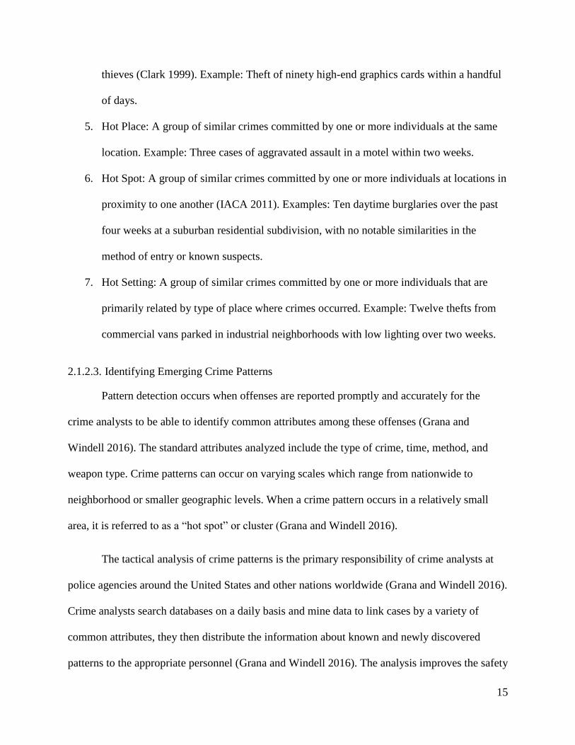
4. Hot Product: A group of crimes committed by one or more individuals in which a unique

type of property is targeted for theft. These are thefts of products deemed attractive to

15

thieves (Clark 1999). Example: Theft of ninety high-end graphics cards within a handful

of days.

5. Hot Place: A group of similar crimes committed by one or more individuals at the same

location. Example: Three cases of aggravated assault in a motel within two weeks.

6. Hot Spot: A group of similar crimes committed by one or more individuals at locations in

proximity to one another (IACA 2011). Examples: Ten daytime burglaries over the past

four weeks at a suburban residential subdivision, with no notable similarities in the

method of entry or known suspects.

7. Hot Setting: A group of similar crimes committed by one or more individuals that are

primarily related by type of place where crimes occurred. Example: Twelve thefts from

commercial vans parked in industrial neighborhoods with low lighting over two weeks.

2.1.2.3. Identifying Emerging Crime Patterns

Pattern detection occurs when offenses are reported promptly and accurately for the

crime analysts to be able to identify common attributes among these offenses (Grana and

Windell 2016). The standard attributes analyzed include the type of crime, time, method, and

weapon type. Crime patterns can occur on varying scales which range from nationwide to

neighborhood or smaller geographic levels. When a crime pattern occurs in a relatively small

area, it is referred to as a “hot spot” or cluster (Grana and Windell 2016).

The tactical analysis of crime patterns is the primary responsibility of crime analysts at

police agencies around the United States and other nations worldwide (Grana and Windell 2016).

Crime analysts search databases on a daily basis and mine data to link cases by a variety of

common attributes, they then distribute the information about known and newly discovered

patterns to the appropriate personnel (Grana and Windell 2016). The analysis improves the safety

16

of communities by shortening police response times and increasing police presence in high crime

areas, which can reduce and prevent crime.

Effectively illustrating the hot spot crime patterns on a map means a crime analyst should

understand the available methodologies and utilize them for different scales of analysis. Eck et

al. (2005) suggest that crime analysts start the search for hot spot crime patterns by plotting

points on small-scale maps, before the examination at larger scales of geography because of

point overlaps. After using a preliminary visual analysis to search for clustered points, incidents

of varying counts and ranges can be represented using different graduated symbols/colors

(Paynich & Hill 2010). This next step of creating a descriptive map through the use of thematic

mapping options is a common method of displaying statistically summarized data to get a more

accurate picture of the overall distribution of crime (Santos 2016; Eck et al. 2005). Following the

descriptive mapping is a form of standard deviation and density mapping analysis. Standard

deviation mapping shows point clusters generated by random chance (Paynich & Hill 2010), and

density mapping uses cells of different radius to perform mathematical functions for surface

estimations which clearly show crime intensities in places containing many overlapping points

(Harris 1999).

Once crime patterns are identified and mapped, they are communicated to police agencies

via a bulletin. The bulletin describes in detail, the critical elements of the crime pattern and

highlights any necessary implications for action. More specifically, crime pattern bulletins

naturally include analytical elements such as a geographic profile, a temporal profile, suspect

lists matching physical, modus operandi (M.O.) descriptions, or other information of

investigative or prescriptive response value (IACA 2011).

17

2.2. Spatial Statistics for Clustering

For the hot streets to be a significant means of crime analysis like the Hot Spots, it has to

utilize a GIS and apply statistical tests (National Institute of Justice 2010). There are several

ways to apply statistics to find spatial clusters, e.g., Moran I statistics, Geary’s C, Getis-Ord Gi,

and Getis-Ord Gi* (Eck et al. 2015; Bruce et al. 2011). Careful consideration needs to be made

in selecting a particular statistic, as methods such as the Moran’s I (either general or local)

cannot tell if the clustering is made of high or low values, it can only sense the presence of

similar clustered values (Chang 2014). The inability of Moran’s I to identify non-similar (high

vs. low) cluster values and the necessity for such an analysis resulted in the use of the Getis-Ord

Gi* statistic that takes account of neighboring features to locate where high and low values

cluster spatially and show local dependence (Getis and Ord, 1993).

Hot Spots are currently created within an ESRI GIS environment using z-scores and p-

values after calculating Getis-Ord Gi* statistic (Esri 2018). The Gi* statistic is used in this study

because it enables the detection of local pockets of dependence not revealed using Moran’s I

statistic alone (Getis and Ord 1993). Ord and Getis (1995) expanded on the created spatial

statistic (Getis and Ord 1993) to show how the mathematics accounts for the distance weights.

The formula which is like that of Figure 2, was suited to study local patterns in spatial data and

was initially tested with AIDS data and outbreaks which proved very useful in creating accurate

Hot Spots.

18

Figure 2. Gi* statistics formula. Source: Esri 2018

Monzur (2015) explained the calculations using the Gi* statistic in step by step order,

which revealed the possible application at street level under a fixed distance analysis, where

connected roads are analyzed for each road crime cluster value. Following the traffic accident

analysis and mapping from Esri (2018b), it was proven that the Hot Spot tool within the Esri GIS

platform could generate both area Hot Spots and linear Hot Spots, which are the same as the Hot

Streets. Given the proven accuracy of using the Hot Spot analysis tool from area to street specific

calculation, it presented the opportunity to create the Hot Streets automatically with a tool

already in the GIS.

2.3. Hot Spot Policing

Hot spot policing has become a common way for police departments to prevent crime

(Braga et al. 2012). Weisburd et al. (2001) explained that in a national survey of police

departments with over 100 officers, 6 in 10 departments reported using crime mapping to

19

visually identify crime Hot Spots for concentrated efforts. The following sections provide

background on advances and advantages of Hot Spot policing as well as the development of Hot

Streets for policing efforts.

2.3.1. Advantages of Hot Spot Policing

Over the recent years, the results of studies suggest that when police focus on smaller

areas where crime is concentrated, they are more efficient at tackling criminal events (Grana and

Windell 2016). The systematic review of Hot Spot Policing, showed adequate support for the

assertion that focused police efforts on hot spots can be effective in preventing crime (Braga

2008; Braga et al. 2012; Eck 1997, 2002; Skogan and Frydl 2004; Weisburd and Eck 2004).

After a review of crime analysis research, Braga et al. (2012) concluded “20 of 25 tests of hot

spot policing interventions reported noteworthy crime and disorder reductions.” The most

extensive practical tests came back with up to a 75% reduction in motor theft within the study

area. Braga et al. (2012) also discovered that not only did Hot Spot Policing have a positive

effect on lower crimes in the area, it also had a positive effect on the community by creating a

safer environment.

Telep and Weisburd (2016) analyzed 17 systematic reviews of policing performed over a

time span of more than 13 years. Systematic reviews are relevant because they have proven to

provide an assured test of strategy effectiveness, which is an essential resource in academia,

criminology, and police practitioner interests (Telep and Weisburd 2016). From these reviews,

they concluded that most of the effective policing strategies regarding crime control concentrated

on small geographic areas (e.g., hot spot policing). Telep and Weisburd (2016) also realized that

converging on a high crime street segment will not just push that hot spot to the next street block

but would most likely cause a diffusion of the crime to nearby areas. This movement of crime to

20

nearby areas is what makes the Gi* statistic discussed earlier in section 2.3 is very important, as

the results for Hot Streets will reflect crime values in relation to nearby areas (streets) that crime

can possibly migrate along.

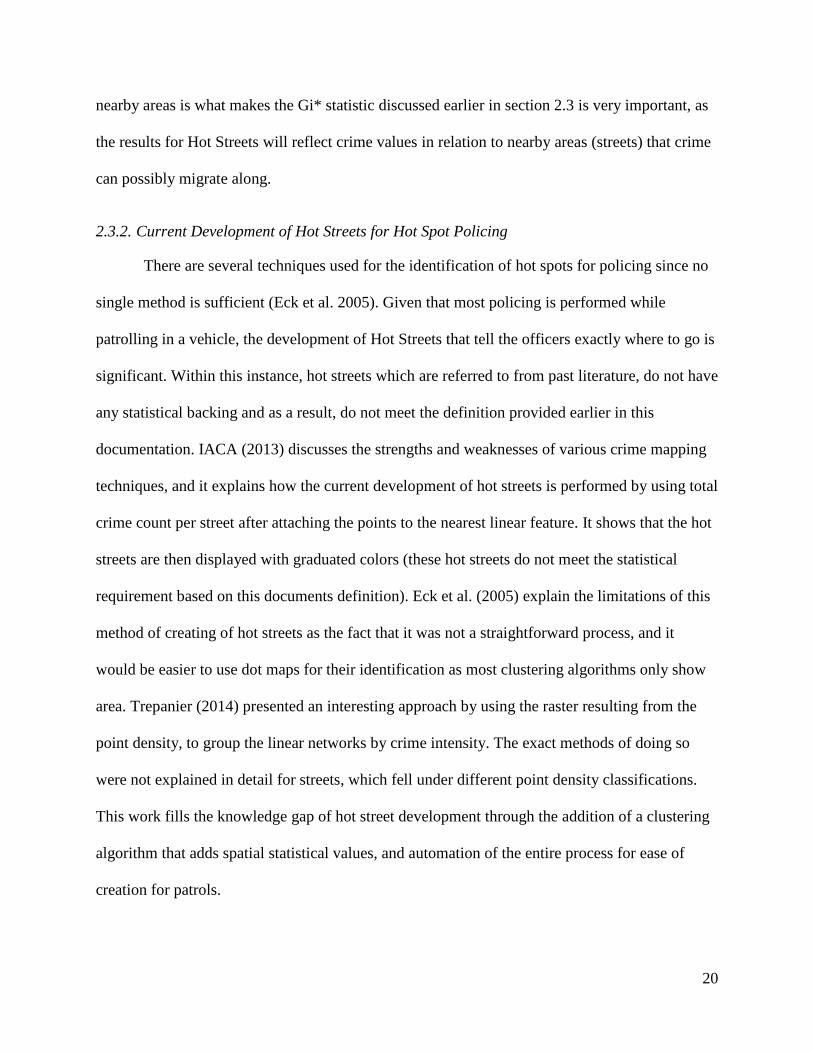
2.3.2. Current Development of Hot Streets for Hot Spot Policing

There are several techniques used for the identification of hot spots for policing since no

single method is sufficient (Eck et al. 2005). Given that most policing is performed while

patrolling in a vehicle, the development of Hot Streets that tell the officers exactly where to go is

significant. Within this instance, hot streets which are referred to from past literature, do not have

any statistical backing and as a result, do not meet the definition provided earlier in this

documentation. IACA (2013) discusses the strengths and weaknesses of various crime mapping

techniques, and it explains how the current development of hot streets is performed by using total

crime count per street after attaching the points to the nearest linear feature. It shows that the hot

streets are then displayed with graduated colors (these hot streets do not meet the statistical

requirement based on this documents definition). Eck et al. (2005) explain the limitations of this

method of creating of hot streets as the fact that it was not a straightforward process, and it

would be easier to use dot maps for their identification as most clustering algorithms only show

area. Trepanier (2014) presented an interesting approach by using the raster resulting from the

point density, to group the linear networks by crime intensity. The exact methods of doing so

were not explained in detail for streets, which fell under different point density classifications.

This work fills the knowledge gap of hot street development through the addition of a clustering

algorithm that adds spatial statistical values, and automation of the entire process for ease of

creation for patrols.

21

Chapter 3 Methodology

This chapter discusses the data, and rationale for the developed Hot Street methodology. Within

this chapter is a detailed explanation of the different data acquired and the variable data types for

the model inputs. After the explanation of the research design, there is a list of data with a

discussion of the fitness for use and processing, before showing the created model.

The primary objective of this project is to create an effective way to allow any user to

accurately represent statistically significant Hot Streets, which previously have proven difficult

to analyze (Eck et al. 2005). The results of this analysis are necessary for reducing the crime

occurrences on dangerous streets, by showing the police departments streets on which they

should concentrate their efforts. The modeling of crime Hot Streets incorporates established

methods and newer analysis techniques that require a wide variety of geoprocessing tools. These

methods formulated after a critical review of relevant literature and informed the development of

the model outlined in this section. The study utilizes spatial data for the model inputs that only

needed a little refinement.

This chapter is subdivided into four sections. The first section elaborates on the research

design and methods acquired from previous researcher. The second section lists out the data

selected and their sources while diving into the fitness of use and preprocessing needs. The third

section presents the flowchart and model that can be replicated to create Hot Streets

automatically.

3.1. Research Design

Early crime street mapping techniques, recommendations from previous research, and

case studies of point to polyline mapping to present a hot street shapefile are the building blocks

22

of this research design. The first step of this thesis project is the combination of the crime points

to the street segments. One recommended option is to plot crime incident locations on a map and

match them to the nearest street layouts based on an approximate distance (IACA 2013; Grana

and Windell 2016). After joining the points to the street segments, there will be a count of points

per street segment. This work builds upon crime mapping on a street level by calculating total

crime count per mile of street to account for different street lengths, instead of using only crime

counts per street. The additional calculation to normalize crimes per mile is crucial because

different streets have different lengths, and smaller streets would most likely have fewer crimes

and vice versa. After calculating the crimes per mile, the Hot Spot analysis tool is run. The Hot

Spot tool operates based on the null hypothesis of complete spatial randomness, and presents

results that reject the null hypothesis and shows the crime patterns. The creation of the spatial

weights matrix file for the scale of analysis and spatial autocorrelation of the data is compulsory

before running the Hot Spot tool. The scale of analysis for this study includes only the

intersecting streets, but it has the potential to include streets connected by drive time, walk time,

or proximity, irrespective of the network connectivity. The spatial autocorrelation is performed

using the Moran’s I statistic to ensure the data shows randomness and clustering, as

demonstrated by a high z-score. With high z-scores that reflect spatial clustering and a small p-

value, the results are statistically significant and mean it is improbable (small probability) that

the observed spatial pattern is the result of random processes. The small p-value rejects the null

hypothesis from the Hot Spot tool, which states that there are noticeable clustering patterns in the

data that the Hot Spot tool can display. Then using the crimes per mile, a Hot Spot analysis will

be run on the linear network dataset, for each connecting street network, ensuring that the model

only takes account of connecting streets to calculate the cluster statistics.

23

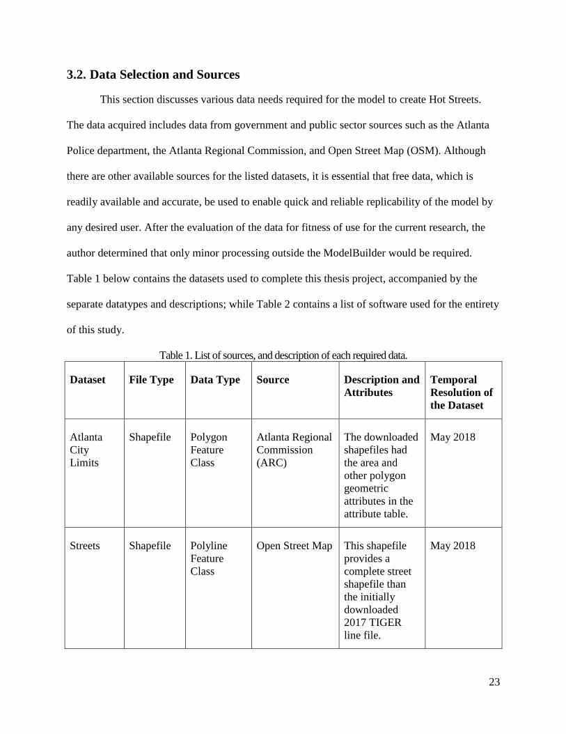
3.2. Data Selection and Sources

This section discusses various data needs required for the model to create Hot Streets.

The data acquired includes data from government and public sector sources such as the Atlanta

Police department, the Atlanta Regional Commission, and Open Street Map (OSM). Although

there are other available sources for the listed datasets, it is essential that free data, which is

readily available and accurate, be used to enable quick and reliable replicability of the model by

any desired user. After the evaluation of the data for fitness of use for the current research, the

author determined that only minor processing outside the ModelBuilder would be required.

Table 1 below contains the datasets used to complete this thesis project, accompanied by the

separate datatypes and descriptions; while Table 2 contains a list of software used for the entirety

of this study.

Table 1. List of sources, and description of each required data.

Dataset File Type Data Type Source Description and

Attributes

Temporal

Resolution of

the Dataset

Atlanta

City

Limits

Shapefile Polygon

Feature

Class

Atlanta Regional

Commission

(ARC)

The downloaded

shapefiles had

the area and

other polygon

geometric

attributes in the

attribute table.

May 2018

Streets Shapefile Polyline

Feature

Class

Open Street Map This shapefile

provides a

complete street

shapefile than

the initially

downloaded

2017 TIGER

line file.

May 2018

24

Dataset File Type Data Type Source Description and

Attributes

Temporal

Resolution of

the Dataset

Crimes Excel.xlxs Point

Feature

Class

Atlanta Police

Department

Data is updated

monthly and is

presented by

Atlanta PD as an

Excel sheet.

2017

Table 2. Summary of Required Software.

Software Manufacturer Function Access

ArcGIS Pro Esri Hot Spot Analysis USC GIST Server

Excel Microsoft View and edit crime

data

Personal Laptop

3.2.1. Atlanta City Limit

The Atlanta city limit was used to set the boundaries needed to crop the streets shapefiles

that fell entirely within the city. The data from the cities regional commission is essential as two

counties currently fall within the boundary of the city.

3.2.1.1. Fitness for Use

The city boundary was fit for use since it accurately represented the city limits through all

the associated counties. The shapefile was used to clip both the crimes dataset and streets data as

the initial crime dataset had features that fell outside the city limits.

3.2.2. Streets

Streets provide the detailed level of analysis which creates Hot Streets, and this is the

critical shapefile required for the model. The streets provide the primary routes of transportation

25

for criminals to get to and away from locations, LEAs to patrol areas and respond to calls, and

civilian’s daily commute to and from their homes. A classification of different street types

already performed on the streets dataset before it was download is accurate enough to eliminate

further attribute table processing. Streets collected as shapefiles from the OSM website

download as a vector polyline that is compatible with Esri products. The Atlanta city limits

extends into two counties but not entirely, so some of the streets had to be cropped at the city

boundary. The projected coordinate system (PCS) used for the final analysis was

NAD_1983_UTM_Zone_16N.

There are eleven attributes for each street segment, notably the street names and street

types/classes. The six important attributes for this analysis include 1) osm_id which is a unique

ID for each linear feature; 2) code and 3) fclass which identify the different road classes, e.g.,

primary, secondary, tertiary, residential, service, and unclassified roads; 4) street names; 5) ref

which contains the alternate state street names (e.g., street name West Hill Avenue is

US84/US221/GA 38 in the ref column); and finally 6) Shape_length in meters.

3.2.2.1. Fitness for Use

The sole purpose of the streets is to spatially represent the crimes, as such the only

criteria needed to determine the fitness of use in this study include spatial accuracy and street

names already provided in the attribute table. The 2018 dataset provided by a credible source

through OSM, has functional overlap with personally tested Orbview-3 satellite imagery

downloaded from the United States Geological Survey (USGS) website. Other credible sources

for this street dataset include the TIGER-Line Files from the U.S Census Bureau, which provided

the base from which OSM created their road shapefiles. OSM streets are initially the 2005

26

TIGER line file from United States Census Bureau, with continual edits from the organization

and volunteer contributions that are verified and approved.

3.2.2.2. Processing

The streets data went through some additional processing once in the model. The streets

were clipped to only show those linear features within the city limits provided by ARC. The

streets dataset was projected to NAD_1983_UTM_Zone_16N, which allowed streets geometry

calculation for the provision of the length of each linear feature. The length is essential because it

was used to determine the ratio of crimes per street, as longer street segments tend to have more

crime. The streets with the added crime ratio were placed as inputs into the Hot Spot analysis

tool to create the Hot Streets. Before running the tool, it is crucial to covert the null values within

the Crimes per Mile (CPM) column to zeros (the rows remained null because when performing a

crime per mile calculation, the streets with zero crime could not be divided to present a result).

Within the Hot Spot tool, the conceptualization of spatial relationships is the spatial weight

matrix file.

3.2.3. Crimes

Crime data was used to show where the offenses occurred along the streets. The crime

data initially came in an excel sheet from the Atlanta police department and consisted of all the

crimes that occurred in the year of 2017. The excel sheet contained the metadata explaining the

different headings and crime types available for download on the police department website. The

crimes were clipped using the Atlanta city limits boundary shapefile, as some police responses

were to nearby cities. The data provided over 26,000 records, of which only ten rape accidents

remained unused due to unavailable locations for privacy reasons. When displayed, the data

showed clusters in downtown that were sufficient enough to be used to find clusters through Hot

27

Spot and Hot Streets. Crime attributes include the: MI_PRINX; offense_id; report date;

occurrence date; Occurrence time; beat; location; MinOfucr and MinOfibr_code which contains

numerical values that group the crimes types; Maximum number of victims; shifts; Average Day;

UC2_Literal contains the crime type; neighborhood; X and Y locations. There are three shift

types with two-hour overlaps for the city of Atlanta, they include the day (6am to 4pm), evening

(2pm to 12am), and morning (10pm to 8am) shift.

3.2.3.1. Fitness for Use

The determining factor with regards to crime data fitness for use is the ability to integrate

it within ArcGIS for quick automated spatial processing. The crimes already have latitude and

longitude positions, which provide a means to integrate the data into the model quickly. The data

is credible as the police department provides it, but there have been concerns about the spatial

accuracy as to where the crimes were reported to occur when attached to the streets. Performing

a random sampling of several crimes to nearest street connections provided a numeric value of

accuracy to address the connection concerns in using personally non-geocoded data. A random

sampling of the 26,318 crimes performed, at 95% confidence level with a 4% interval needs a

sample size of 579. The random sampling shows that slightly over 81% of the data matched to

the right streets, eliminating the need to geocode the dataset for this project. Most of the issues

from the remaining 19% resulted from crimes at intersection points, or neighboring streets of

buildings with two exits to both roads, which do not cause a significant impact in the data for this

level of analysis because the analysis weighs connecting streets in the calculations. A Sergeant

within the Tactical Crime Analysis Unit in the Atlanta PD provided assurances that the geocoded

data by the police department is accurate since they place each point on the proper building/ edge

28

of the road (Petersen, Robert E. Personal interview. 11 April 2018). The current data attributes as

can be seen from Figure 3, which show the crime locations and streets names match nicely.

Figure 3. Screenshot of crime locations (left) and the associated street names (right) from a

random sampling across the full dataset

3.2.3.2. Processing

The crimes required pre-processing outside the model. They were given the same

projection as the streets layer, then snapped to the closest roads. After the point snaps, each

crime is associated with the closest street and summarized into the street layer table via a total

count. The data went on to be processed on the street level to create Hot Streets. The crime point

data is also an input for the Point Density tool and the Kernel Density tool, to compare the results

of the model to current predominant crime analysis techniques. The Kernel Density tool

calculates the density of features in a neighborhood around those features, while the point

density tool calculates the density of point features around each output raster cell. Both density

tools are used to create density crime reports.

29

3.3. GIS Procedures and Analysis Models

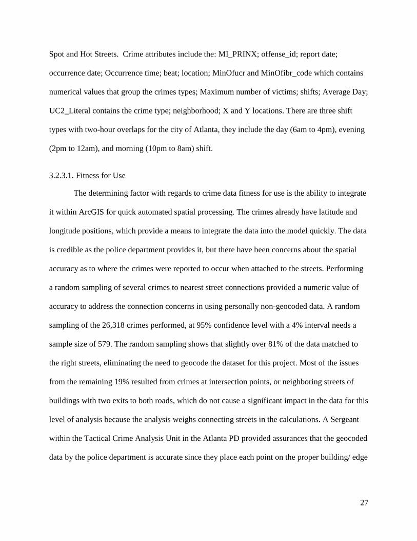
After gathering a general understanding of the appropriate approaches, a flowchart was

developed to show the primary sequence of events (Figure 4). The simple flowchart can help

users of other GIS software to see the needed steps quickly.

The flowchart from the research design in Figure 4 results in a different sequence of

events due to the accumulation of tools grouped into different sections within the GIS

ModelBuilder. Based on the model processing requirements, there will be seven main groups.

3.3.1. Select City Streets Excluding Expressways

The extraction of the needed street layer within the study area is the first step of the

analysis, and will make the first group. Open street maps are usually downloaded for the entire

state, using the city limits shapefile to clip the extents will provide the streets within the city

limits alone. Following the creation of the street layer within the study area, is the removal of

express lanes and exit ramps as highways are patrolled differently, and are not always connected

to neighboring streets. Also, only a handful of crimes happened on them. Four tools were used in

this process 1) Clip tool to create the Atlanta city streets, 2) the Make Feature Layer tool to

create a layer that could be used by the 3) Select Layer by Attribute tool for inverse selection of

expressways and exit ramps, and finally 4) the Copy Features tool that extracts the selected

streets.

30

Figure 4. Flowchart of Hot Street Model

31

3.3.2. Select Crime Type and Shift

In tactical crime analysis situations, most of the analysis is performed in real time and for

the purpose of briefing officers coming in at different shifts. Providing the option to analyze

different crime types that occur during different shifts can help the incoming officers gain a

better understanding of the current crime patterns and streets on which they occur. The two tools

used within this group are the 1) Select Layer By Attribute which will show the expression as a

parameter for different selection types, and the 2) Table Select tool used for the extracting the

needed data for analysis.

3.3.3. Show Selected Crimes within the City

With the latitude and longitude information within the table, the point layers that fall

within the city are developed. The data will not provide locations for rape, as there are no

locations for privacy reasons. The two tools used in this grouped analysis are 1) Make XY Event

Layer to create the shapefiles from the table, and 2) Clip tool for selecting only crimes within the

city limits.

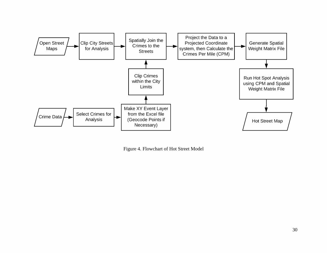
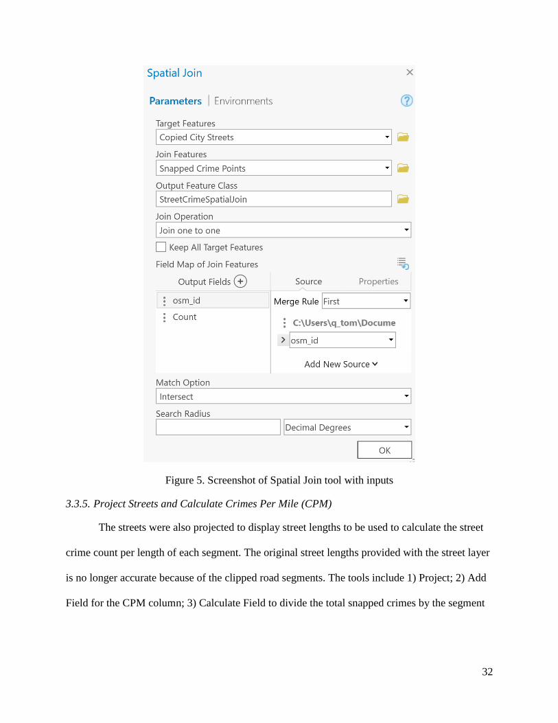
3.3.4. Spatial Join

This purpose of this grouped set of tools is the combination of the crime counts to the

street layer. The same process was used by Dr. Lixin Huang (Esri, 2018b) in analyzing traffic

accidents with 1) the Snap tool which joins the crimes to the nearest roads, and 2) the spatial join

tool seen with the parameters in Figure 5.

32

Figure 5. Screenshot of Spatial Join tool with inputs

3.3.5. Project Streets and Calculate Crimes Per Mile (CPM)

The streets were also projected to display street lengths to be used to calculate the street

crime count per length of each segment. The original street lengths provided with the street layer

is no longer accurate because of the clipped road segments. The tools include 1) Project; 2) Add

Field for the CPM column; 3) Calculate Field to divide the total snapped crimes by the segment

33

lengths. The following section changes the NULLs into Zeros and reselects all layers otherwise

the Generate Spatial Weight Matric File will not incorporate all the streets within the city streets.

3.3.6. Generate Spatial Weight Matrix (SWM) File

This portion of the model runs with seven different tools to generate the spatial weight

matrix. Without this spatial weight matrix that tells the Hot Spot tool the neighboring features,

the Hot Spot tool will select roads that do not intersect and may not have connectivity when

looking at the street routes. The neighboring issue arises because the Hot Spot analysis tool is

initially for only point and polygon layers.

The first performed function is the generation of a table with nearby streets by

intersection with the Generate Near Table or the Summarize Nearby tool (Figure 6). The

Summarize Nearby tool was tested but not used in the final model because of the 20 minute run

time for this geoprocessing tool alone.

34

Figure 6. Screenshots of tools used to generate a near table for the SWM file

35

Next, the summarize Nearby tool creates the table, all distance types except straight-line

distance use ArcGIS Online routing and network services. The distance measurement types

include 1) Driving Distance; 2) Driving Time; 3) Straight Line; 4) Trucking Distance; 5)

Trucking Time; 6) Walking Distance; 7) Walking Time. The distance types create polygons of

buffers in a single table, which meet the required distance or drive time. The drive distance and

time use the road network and obey all connectivity and speed limit rules. The drive-time and

drive distance measurement options are not necessary for the development of this model but

should others want to run drive-time, they must ensure that they have the appropriate license and

credits.

36

Figure 7. Altered fields after the generated nearby table.

After the table with the connected streets is created, the fields are altered (Figure 8) to

meet the requirement for the Generate Spatial Weights Matrix tool. The tool requires three fields

which include the OBJECTID; the UniqueID renamed as whatever unique numeric column for

each row within the streets layer, the Near ID (NID) which holds the connected UniqueID

37

values, and finally the WEIGHT. The created table is used to generate the .SWM file needed as

an input table for Hot Spot Analysis tool as can be seen in Figure 8.

Figure 8. Generate Spatial Weights Matrix tool

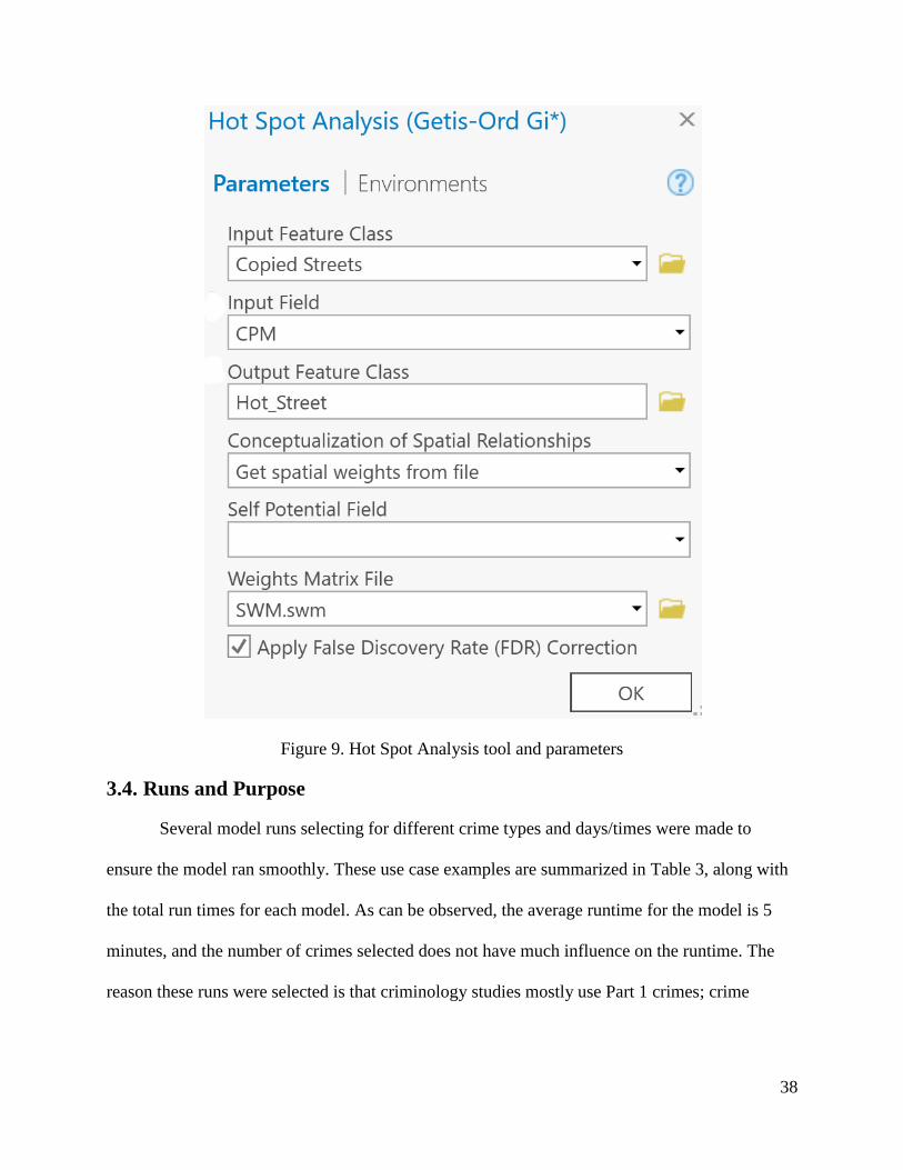
3.3.7. Spatial Autocorrelation

The Moran’s I statistic was performed before the Hot Spot tool to ensure there is perfect

randomness in the data after given a set of weighted features. The Hot Spot tool (Figure 9)

identifies statistically significant spatial clusters of high values (Hot Spots) and low values (Cold

Spots) with the Getis-Ord Gi* statistic. It creates a new Output Feature Class with a z-score, p-

value, number of neighbors, and confidence level bin (Gi_Bin) for each feature in the Input

Feature Class.

38

Figure 9. Hot Spot Analysis tool and parameters

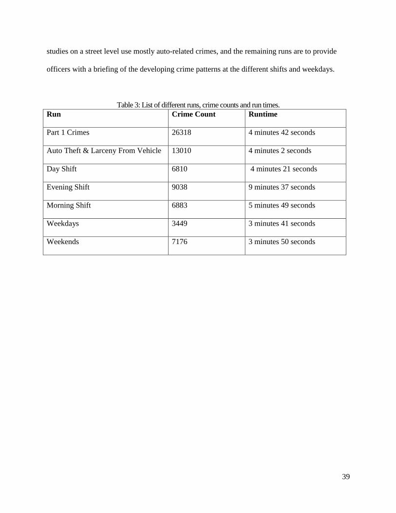
3.4. Runs and Purpose

Several model runs selecting for different crime types and days/times were made to

ensure the model ran smoothly. These use case examples are summarized in Table 3, along with

the total run times for each model. As can be observed, the average runtime for the model is 5

minutes, and the number of crimes selected does not have much influence on the runtime. The

reason these runs were selected is that criminology studies mostly use Part 1 crimes; crime

39

studies on a street level use mostly auto-related crimes, and the remaining runs are to provide

officers with a briefing of the developing crime patterns at the different shifts and weekdays.

Table 3: List of different runs, crime counts and run times.

Run Crime Count Runtime

Part 1 Crimes 26318 4 minutes 42 seconds

Auto Theft & Larceny From Vehicle 13010 4 minutes 2 seconds

Day Shift 6810 4 minutes 21 seconds

Evening Shift 9038 9 minutes 37 seconds

Morning Shift 6883 5 minutes 49 seconds

Weekdays 3449 3 minutes 41 seconds

Weekends 7176 3 minutes 50 seconds

40

Chapter 4 Results

Chapter 4 documents the results of the final Hot Street model. This chapter is broken into three

sections to present the results of the analysis. Section 4.1 provides the Hot Street Model. Section

4.2 displays the results from the spatial autocorrelation. Section 4.3 displays the number of Hot

Streets generated from each model run, with maps that display the locations in the city.

4.1. Hot Street Model

After performing several runs, the final model and parameters for the geoprocessing pane is

finished and can be seen in Figures 10 and 11 with all the processing groups. There are a total

number of 11 groups which execute different functions in the model, and nine parameters (see

Appendix A for detailed sections of the Hot Street Model). The input parameters are displayed in

a blue background for the layers, and white for the expression. The tools are displayed with a

yellow background, while the outputs from the tools are shown with a green background. The

first group consists of the model parameters and expression for the crime selection, which also

appear in Figure 10. The other groups, as stated in the methodology, follow after the input

parameters group and before the final result is displayed. Due to the number of tools used, setting

preconditions is important for output results that are used as different tool inputs so that there

will be a proper progression of analysis with no errors. After showing the created maps, the Hot

Streets are hard to visually see since this level of analysis provides more specific results over

larger geographic scales. The symbology is updated within the model to present statistically

significant Hot Streets with thicker widths for quick identification.

41

Figure 10. Hot Street Model as Geoprocessing Tool

42

Figure 11. Hot Street Model

43

4.2. Spatial Autocorrelation

To ensure the spatial weight matrix contained a minimum of one neighbor is a scale of analysis

with data that is randomly dispersed, the Moran’s I tool is run before the Hot Spot Analysis. The

Getis-Ord General G statistic is not used with the Gi* statistic because when the high and low

values cluster, they cancel out (Esri 2018c). For this reason, the Moran’s I spatial autocorrelation

tool is used to measure the spatial clustering of where both the high values and low values

cluster. Table 4 contains the results generated from the spatial autocorrelation tool. The high z-

scores indicate there is clustering and less than 1% likelihood that the pattern is a result of

random chance. The Moran’s I values close to 0 indicate a pattern of perfect randomness.

Table 4. Moran’s I Results

Run Z-Score Moran’s I

Part 1 Crimes 8.767995 0.039697

Auto Theft & Larceny From Vehicle 7.238768 0.031967

Day Shift 7.729909 0.034891

Evening Shift 4.574907 0.030494

Morning Shift 16.784498 0.076841

Weekdays 8.795830 0.040214

Weekends 20.740992 0.094857

4.3. Hot Street Result

After creating the final model, all seven runs displayed different Hot Streets. The resultant Hot

Streets are categorized into three different confidence levels at 90%, 95%, 99%. The different

confidence levels are classified based on the z-scores and p-values. A 90% confidence level has a

44

p-value < 0.10 and a z-score < -1.65 or > +1.65, a 95% confidence level has a p-value < 0.05

and a z-score < -1.96 or > +1.96, and the 99% confidence level has a p-value < 0.01 and a z-

score < -2.58 or > +2.58. Table 5 shows the total number of Hot Streets generated from each

model run for different street classes and CLs. Service roads had the highest number of Hot

Streets for every run, followed by residential then tertiary or secondary roads.

Eight maps are created from the Hot Street model, the maps from the different runs can

be seen from Figures 12 to 20. The Hot Street maps are placed over the kernel density results to

show that the streets are mostly located in portions of the map that overlap with high density of

crime. Each section with a map developed from the model contains two sections for the results.

The first paragraph lists out the total number of Hot Streets at each confidence level (CL) for the

different street classes. The second paragraph contains a total number of Hot Streets at different

CL that overlaps with the different kernel density classes (generated using Jenks normal break

classification).

45

Table 5. Number of Hot Streets generated from the model.

Number of Hot Streets

Street Class Primary Secondary Tertiary Residential Service Unclassified Total

CL (%) 90 95 99 90 95 99 90 95 99 90 95 99 90 95 99 90 95 99

Part 1 Crimes _ _ 1 4 2 6 _ 2 6 4 7 19 26 56 280 _ _ _ 413

Auto Theft & Larceny

From Vehicle _ 1 _ _ 1 5 1 1 4 2 7 15 26 41 218 _ _ _ 322

Day Shift _ _ 1 2 4 4 _ _ 6 1 3 16 30 41 225 _ _ _ 333

Evening Shift _ 1 _ 3 2 5 _ 1 6 1 3 10 40 37 264 _ _ _ 373

Morning Shift _ _ 3 2 3 5 _ 3 3 8 3 20 23 47 242 _ 1 2 365

Weekdays _ _ _ 5 1 6 1 1 6 3 2 18 28 71 325 _ _ _ 467

Weekends _ _ 2 2 4 5 _ 1 2 3 5 29 37 59 275 _ _ 1 425

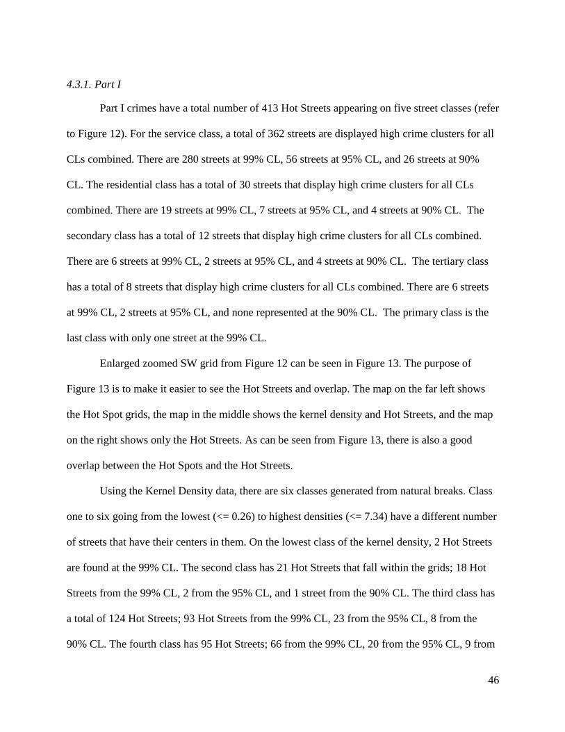
46

4.3.1. Part I

Part I crimes have a total number of 413 Hot Streets appearing on five street classes (refer

to Figure 12). For the service class, a total of 362 streets are displayed high crime clusters for all

CLs combined. There are 280 streets at 99% CL, 56 streets at 95% CL, and 26 streets at 90%

CL. The residential class has a total of 30 streets that display high crime clusters for all CLs

combined. There are 19 streets at 99% CL, 7 streets at 95% CL, and 4 streets at 90% CL. The

secondary class has a total of 12 streets that display high crime clusters for all CLs combined.

There are 6 streets at 99% CL, 2 streets at 95% CL, and 4 streets at 90% CL. The tertiary class

has a total of 8 streets that display high crime clusters for all CLs combined. There are 6 streets

at 99% CL, 2 streets at 95% CL, and none represented at the 90% CL. The primary class is the

last class with only one street at the 99% CL.

Enlarged zoomed SW grid from Figure 12 can be seen in Figure 13. The purpose of

Figure 13 is to make it easier to see the Hot Streets and overlap. The map on the far left shows

the Hot Spot grids, the map in the middle shows the kernel density and Hot Streets, and the map

on the right shows only the Hot Streets. As can be seen from Figure 13, there is also a good

overlap between the Hot Spots and the Hot Streets.

Using the Kernel Density data, there are six classes generated from natural breaks. Class

one to six going from the lowest (<= 0.26) to highest densities (<= 7.34) have a different number

of streets that have their centers in them. On the lowest class of the kernel density, 2 Hot Streets

are found at the 99% CL. The second class has 21 Hot Streets that fall within the grids; 18 Hot

Streets from the 99% CL, 2 from the 95% CL, and 1 street from the 90% CL. The third class has

a total of 124 Hot Streets; 93 Hot Streets from the 99% CL, 23 from the 95% CL, 8 from the

90% CL. The fourth class has 95 Hot Streets; 66 from the 99% CL, 20 from the 95% CL, 9 from

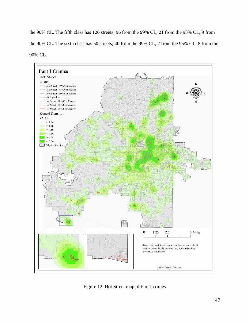
47

the 90% CL. The fifth class has 126 streets; 96 from the 99% CL, 21 from the 95% CL, 9 from

the 90% CL. The sixth class has 50 streets; 40 from the 99% CL, 2 from the 95% CL, 8 from the

90% CL.

Figure 12. Hot Street map of Part I crimes

48

Figure 13. Zoomed in SW section of the Part I Hot Street Map

49

4.3.2. Auto Theft

Auto theft and vehicle larceny crimes have a total of 322 Hot Streets appearing on five

street classes (Figure 14). For the service class, a total of 285 streets are displayed high crime

clusters for all CLs combined. There are 218 streets at 99% CL, 41 streets at 95% CL, and 26

streets at 90% CL. The residential class has a total of 24 streets that display high crime clusters

for all CLs combined. There are 15 streets at 99% CL, 7 streets at 95% CL, and 2 streets at 90%

CL. The secondary class has a total of 6 streets that display high crime clusters for all CLs

combined. There are 5 streets at 99% CL, 1 streets at 95% CL, and no streets at 90% CL. The

tertiary class has a total of 6 streets that display high crime clusters for all CLs combined. There

are 4 streets at 99% CL, 1 streets at 95% CL, and 1 street represented at the 90% CL. The

primary class is the last class with only one street at the 95% CL.

Using the Kernel Density Data, there are six classes generated from a natural breaks.

Class one to six going from the lowest (<= 0.11) to highest (<= 3.55) densities. On the lowest

class of the kernel density, no Hot Streets are found. The second class has 21 Hot Streets that fall

within the grids; 19 Hot Streets from the 99% CL, 1 from the 95% CL, and 1 street from the 90%

CL. The third class has a total of 66 Hot Streets; 50 Hot Streets from the 99% CL, 12 from the

95% CL, 4 from the 90% CL. The fourth class has 91 Hot Streets; 61 from the 99% CL, 20 from

the 95% CL, 10 from the 90% CL. The fifth class has 104 streets; 80 from the 99% CL, 14 from

the 95% CL, 10 from the 90% CL. The sixth class has 44 streets; 35 from the 99% CL, 4 from

the 95% CL, 5 from the 90% CL.

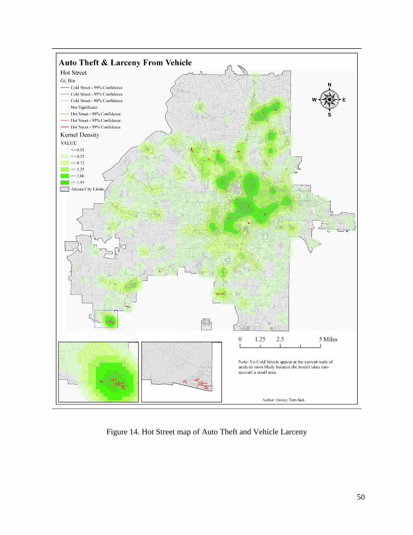
50

Figure 14. Hot Street map of Auto Theft and Vehicle Larceny

51

4.3.3. Day Shift

Day shift crimes have a total of 333 Hot Streets appearing on five street classes (Figure

15). For the service class, a total of 296 streets are displayed high crime clusters for all CLs

combined. There are 225 streets at 99% CL, 41 streets at 95% CL, and 30 streets at 90% CL. The

residential class has a total of 20 streets that display high crime clusters for all CLs combined.

There are 16 streets at 99% CL, 3 streets at 95% CL, and 1 streets at 90% CL. The secondary

class has a total of 10 streets that display high crime clusters for all CLs combined. There are 4

streets at 99% CL, 4 streets at 95% CL, and 2 streets at 90% CL. The tertiary class has a total of

6 streets that display high crime clusters at 99% CL. The primary class is the last class with only

1 street at the 99% CL.

Using the Kernel Density Data, there are six classes generated from a normal density.

Class one to six going from the lowest (<=0.06) to highest (<=1.59) densities. On the lowest

class of the kernel density, no Hot Streets are found. The second class has 28 Hot Streets that fall

within the grids; 24 Hot Streets from the 99% CL, 2 from the 95% CL, and 2 street from the 90%

CL. The third class has a total of 93 Hot Streets; 68 Hot Streets from the 99% CL, 11 from the

95% CL, 14 from the 90% CL. The fourth class has 94 Hot Streets; 69 from the 99% CL, 16

from the 95% CL, 9 from the 90% CL. The fifth class has 72 streets; 52 from the 99% CL, 15

from the 95% CL, 5 from the 90% CL. The sixth class has 51 streets; 43 from the 99% CL, 5

from the 95% CL, 3 from the 90% CL.

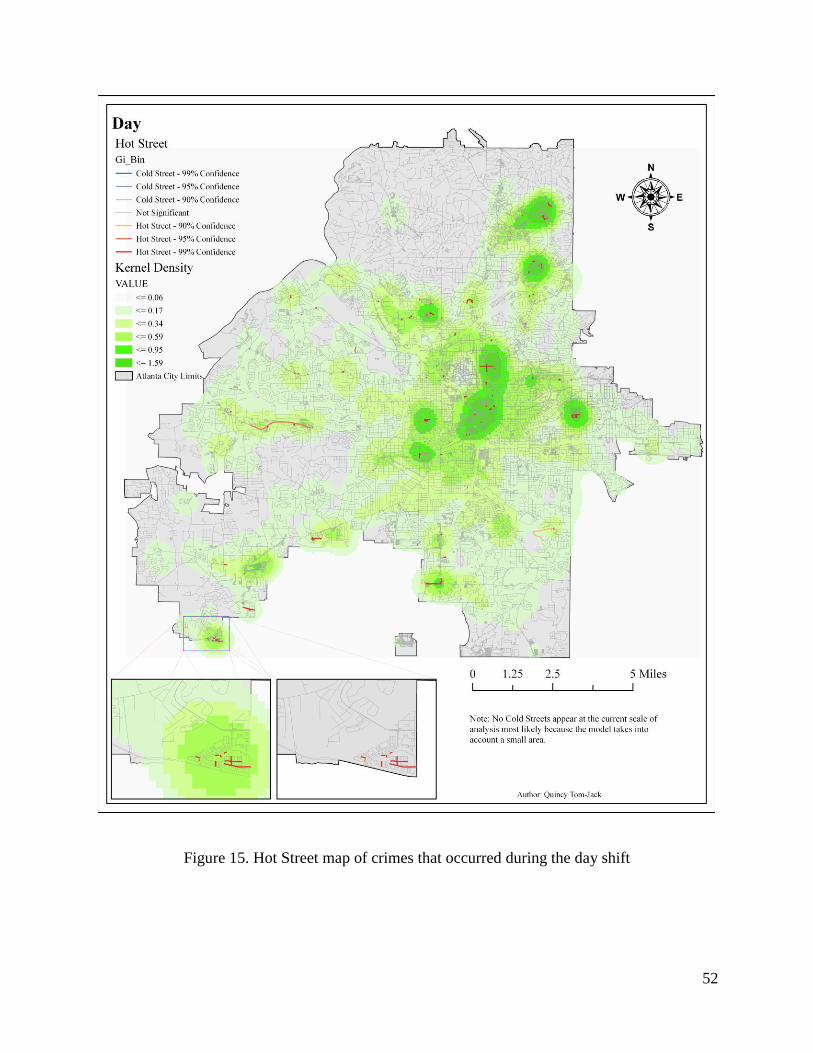
52

Figure 15. Hot Street map of crimes that occurred during the day shift

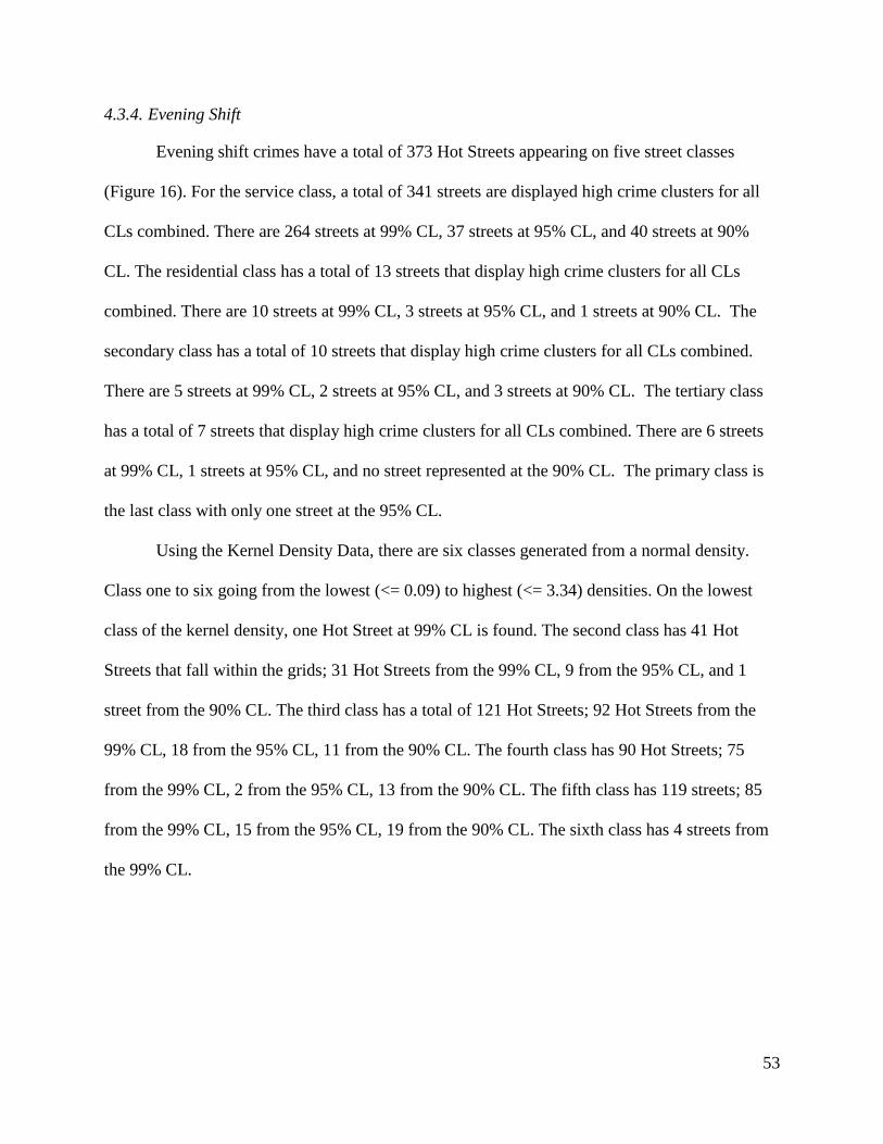
53

4.3.4. Evening Shift

Evening shift crimes have a total of 373 Hot Streets appearing on five street classes

(Figure 16). For the service class, a total of 341 streets are displayed high crime clusters for all

CLs combined. There are 264 streets at 99% CL, 37 streets at 95% CL, and 40 streets at 90%

CL. The residential class has a total of 13 streets that display high crime clusters for all CLs

combined. There are 10 streets at 99% CL, 3 streets at 95% CL, and 1 streets at 90% CL. The

secondary class has a total of 10 streets that display high crime clusters for all CLs combined.

There are 5 streets at 99% CL, 2 streets at 95% CL, and 3 streets at 90% CL. The tertiary class

has a total of 7 streets that display high crime clusters for all CLs combined. There are 6 streets

at 99% CL, 1 streets at 95% CL, and no street represented at the 90% CL. The primary class is

the last class with only one street at the 95% CL.

Using the Kernel Density Data, there are six classes generated from a normal density.

Class one to six going from the lowest (<= 0.09) to highest (<= 3.34) densities. On the lowest

class of the kernel density, one Hot Street at 99% CL is found. The second class has 41 Hot

Streets that fall within the grids; 31 Hot Streets from the 99% CL, 9 from the 95% CL, and 1

street from the 90% CL. The third class has a total of 121 Hot Streets; 92 Hot Streets from the

99% CL, 18 from the 95% CL, 11 from the 90% CL. The fourth class has 90 Hot Streets; 75

from the 99% CL, 2 from the 95% CL, 13 from the 90% CL. The fifth class has 119 streets; 85

from the 99% CL, 15 from the 95% CL, 19 from the 90% CL. The sixth class has 4 streets from

the 99% CL.

54

Figure 16. Hot Street map of crimes that occurred during the evening shift

55

4.3.5. Morning Shift

Morning shift crimes have a total of 365 Hot Streets appearing on five street classes

(Figure 17). For the service class, a total of 312 streets are displayed high crime clusters for all

CLs combined. There are 242 streets at 99% CL, 47 streets at 95% CL, and 23 streets at 90%

CL. The residential class has a total of 31 streets that display high crime clusters for all CLs

combined. There are 20 streets at 99% CL, 3 streets at 95% CL, and 8 streets at 90% CL. The

secondary class has a total of 10 streets that display high crime clusters for all CLs combined.

There are 5 streets at 99% CL, 3 streets at 95% CL, and 2 streets at 90% CL. The tertiary class

has a total of 6 streets that display high crime clusters for all CLs combined. There are 3 streets

at 99% CL, 3 streets at 95% CL, and no street represented at the 90% CL. The primary with 3

streets at the 99% CL, and the Unclassified class with 3 total streets of which 2 are at 99% CL

and 1 street at 95% CL.

Using the Kernel Density Data, there are six classes generated from a normal density.

Class one to six going from the lowest (<= 0.06) to highest (<=1.36) densities. On the lowest

class of the kernel density, 2 Hot Streets are found, 1 for both the 99% and 95% CL. The second

class has 35 Hot Streets that fall within the grids; 24 Hot Streets from the 99% CL, 7 from the

95% CL, and 4 street from the 90% CL. The third class has a total of 93 Hot Streets; 71 Hot

Streets from the 99% CL, 14 from the 95% CL, 8 from the 90% CL. The fourth class has 110

Hot Streets; 86 from the 99% CL, 15 from the 95% CL, 9 from the 90% CL. The fifth class has

56 streets; 42 from the 99% CL, 11 from the 95% CL, 3 from the 90% CL. The sixth class has 73

streets; 53 from the 99% CL, 11 from the 95% CL, 9 from the 90% CL.

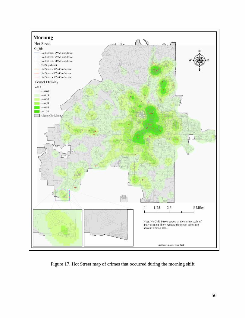
56

Figure 17. Hot Street map of crimes that occurred during the morning shift

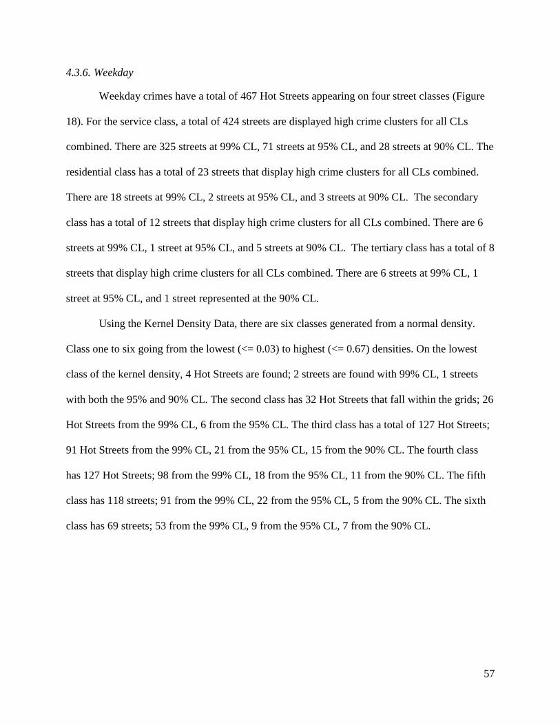
57

4.3.6. Weekday

Weekday crimes have a total of 467 Hot Streets appearing on four street classes (Figure

18). For the service class, a total of 424 streets are displayed high crime clusters for all CLs

combined. There are 325 streets at 99% CL, 71 streets at 95% CL, and 28 streets at 90% CL. The

residential class has a total of 23 streets that display high crime clusters for all CLs combined.

There are 18 streets at 99% CL, 2 streets at 95% CL, and 3 streets at 90% CL. The secondary

class has a total of 12 streets that display high crime clusters for all CLs combined. There are 6

streets at 99% CL, 1 street at 95% CL, and 5 streets at 90% CL. The tertiary class has a total of 8

streets that display high crime clusters for all CLs combined. There are 6 streets at 99% CL, 1

street at 95% CL, and 1 street represented at the 90% CL.

Using the Kernel Density Data, there are six classes generated from a normal density.

Class one to six going from the lowest (<= 0.03) to highest (<= 0.67) densities. On the lowest

class of the kernel density, 4 Hot Streets are found; 2 streets are found with 99% CL, 1 streets

with both the 95% and 90% CL. The second class has 32 Hot Streets that fall within the grids; 26

Hot Streets from the 99% CL, 6 from the 95% CL. The third class has a total of 127 Hot Streets;

91 Hot Streets from the 99% CL, 21 from the 95% CL, 15 from the 90% CL. The fourth class

has 127 Hot Streets; 98 from the 99% CL, 18 from the 95% CL, 11 from the 90% CL. The fifth

class has 118 streets; 91 from the 99% CL, 22 from the 95% CL, 5 from the 90% CL. The sixth

class has 69 streets; 53 from the 99% CL, 9 from the 95% CL, 7 from the 90% CL.

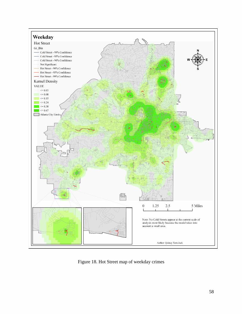
58

Figure 18. Hot Street map of weekday crimes

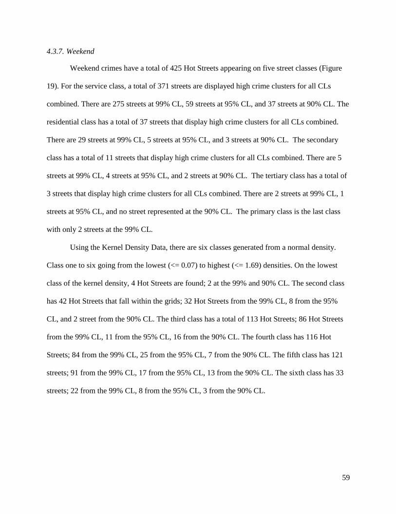
59

4.3.7. Weekend

Weekend crimes have a total of 425 Hot Streets appearing on five street classes (Figure

19). For the service class, a total of 371 streets are displayed high crime clusters for all CLs

combined. There are 275 streets at 99% CL, 59 streets at 95% CL, and 37 streets at 90% CL. The

residential class has a total of 37 streets that display high crime clusters for all CLs combined.

There are 29 streets at 99% CL, 5 streets at 95% CL, and 3 streets at 90% CL. The secondary

class has a total of 11 streets that display high crime clusters for all CLs combined. There are 5

streets at 99% CL, 4 streets at 95% CL, and 2 streets at 90% CL. The tertiary class has a total of

3 streets that display high crime clusters for all CLs combined. There are 2 streets at 99% CL, 1

streets at 95% CL, and no street represented at the 90% CL. The primary class is the last class

with only 2 streets at the 99% CL.

Using the Kernel Density Data, there are six classes generated from a normal density.

Class one to six going from the lowest (<= 0.07) to highest (<= 1.69) densities. On the lowest

class of the kernel density, 4 Hot Streets are found; 2 at the 99% and 90% CL. The second class

has 42 Hot Streets that fall within the grids; 32 Hot Streets from the 99% CL, 8 from the 95%

CL, and 2 street from the 90% CL. The third class has a total of 113 Hot Streets; 86 Hot Streets

from the 99% CL, 11 from the 95% CL, 16 from the 90% CL. The fourth class has 116 Hot

Streets; 84 from the 99% CL, 25 from the 95% CL, 7 from the 90% CL. The fifth class has 121

streets; 91 from the 99% CL, 17 from the 95% CL, 13 from the 90% CL. The sixth class has 33

streets; 22 from the 99% CL, 8 from the 95% CL, 3 from the 90% CL.

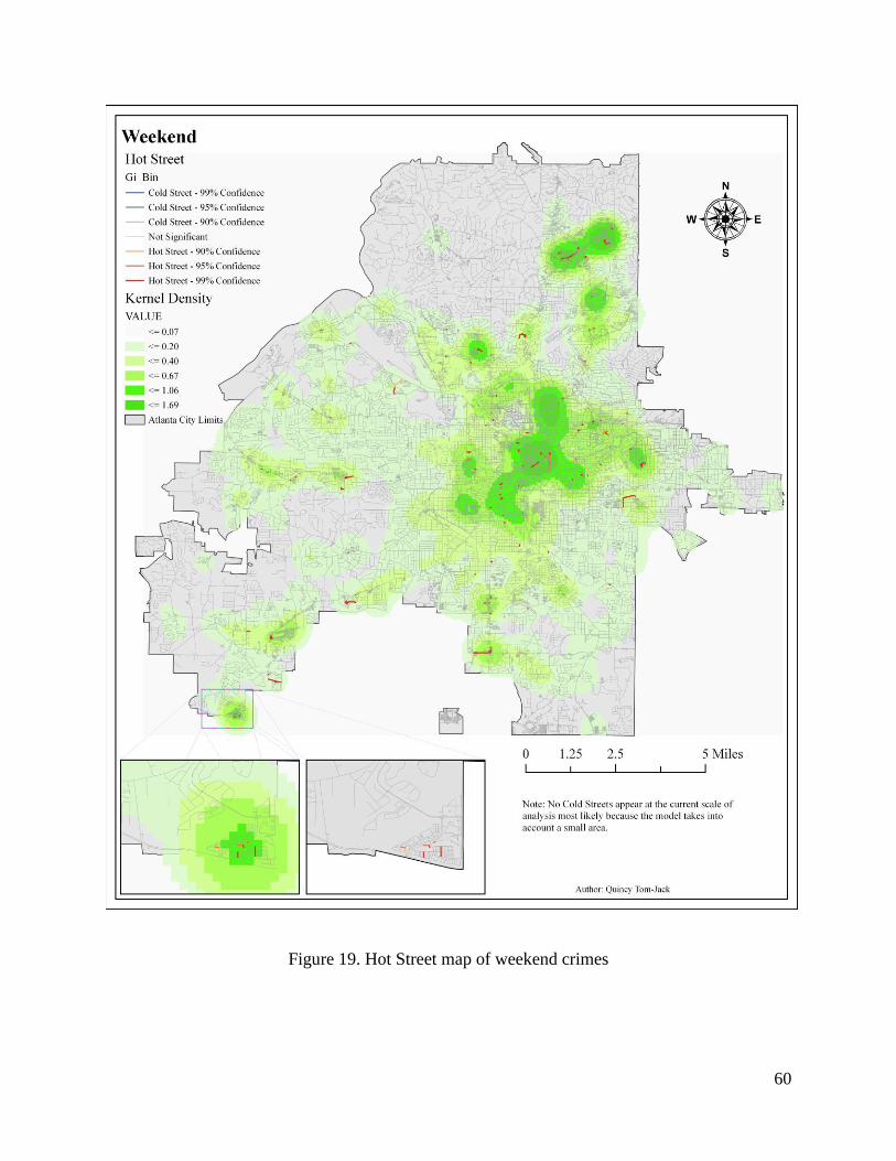
60

Figure 19. Hot Street map of weekend crimes

61

4.3.8. Part I Houston, Texas.

An additional run was performed to test the models ability to run in different cities. Houston,

Texas was chosen because of the available data provided by the City of Houston for all model

parameters. The crime data ranges from July, 2018 to August 20, 2018. Houston Part I crimes

have a total of 910 Hot Streets appearing on five street classes (Figure 20). For the service class,

a total of 153 streets are displayed high crime clusters for all CLs combined. There are 134

streets at 99% CL, 14 streets at 95% CL, and 5 streets at 90% CL. The residential class has a

total of 76 streets that display high crime clusters for all CLs combined. There are 61 streets at

99% CL, 10 streets at 95% CL, and 5 streets at 90% CL. The secondary class has a total of 460

streets that display high crime clusters for all CLs combined. There are 385 streets at 99% CL,

51 streets at 95% CL, and 24 streets at 90% CL. The tertiary class has a total of 83 streets that

display high crime clusters for all CLs combined. There are 67 streets at 99% CL, 9 streets at

95% CL, and 7 at the 90% CL. The primary class has a total of 125 streets. There are 105 streets

at the 99% CL, 14 streets at the 95% CL, and 6 streets at the 90% CL. There are 13 unclassified

Hot Streets. 11 of which fall into the 99% CL, and 1 in both the 95% and 90% CL.

Using the Kernel Density Data, there are six classes generated from a normal density.

Class one to six going from the lowest (<= 0.09) to highest (<= 3.39) densities. On the lowest

class of the kernel density, 13 Hot Streets are found in total; 8 at the 99% CL, 3 at the 95% CL,

2 at the 90% CL. The second class has 80 Hot Streets that fall within the grids; 64 Hot Streets

from the 99% CL, 8 from the 95% CL, and 8 street from the 90% CL. The third class has a total

of 325 Hot Streets; 282 Hot Streets from the 99% CL, 28 from the 95% CL, 15 from the 90%

CL. The fourth class has 340 Hot Streets; 280 from the 99% CL, 39 from the 95% CL, 21 from

the 90% CL. The fifth class has 186 streets; 165 from the 99% CL, 16 from the 95% CL, 5 from

62

the 90% CL. The sixth class has 63 streets; 47 from the 99% CL, 13 from the 95% CL, 3 from

the 90% CL.

Figure 20. Part I Hot Street of Central Houston, Texas

63

Chapter 5 Discussion and Conclusions

The model is successful in providing an effective way to depict Hot Streets, despite all

the challenges faced. This chapter discusses the key findings and possible impact of the findings,

as well as the research limitations and future research.

5.1. Findings and Impact

5.1.1. Model

Through the course of developing this model, it was discovered that the model could easily be

replicated for different scales that utilize street attributes to change the number of influencing

street segments. After the first run, the model time can be improved by removing some of the

tools that would provide the same output despite the change in crime selection. The removal of

some of the grouped processes and tools can be adjusted to suit the efficient needs of the analyst

or researcher if the study is performed over the same area on multiple runs. After the first run,

the first group that can be removed is the Select City Streets group if the study area remains the

same. With the same study area, there is no need to create the same street layer for snapping

features continuously. The second group that can be changed is the Generate Spatial Weight

Matrix File group. Within the group, the spatial weight matrix input table is created with the first

five tools. The table can remain the same if the output street layer at the end of the Select City

Streets remains unchanged, and the scale of analysis is the same. This is because the street ID is

used to distinguish each linear feature and the streets included for the spatial statistics.

The model takes a considerable amount of time to run, the average time of the model

when using the Generate Near Table tool to create the spatial weight matrix input table is 5

minutes. If the Summarize Nearby tool is used to create the spatial weight input table, the

runtime for the same scale of analysis will be increased by approximately 25 minutes, to bring

64

the full model runtime to an average of 30 minutes. If more complex distance units such as the

travel time are used, the time can scale up to an hour or more for each individual run. It is

recommended that if the Summarize Nearby tool is used, the spatial weight matrix should be

prebuilt using ranges of drive time or distance, e.g., 5 minutes, 15 minutes, 30 minutes, and so

on. The other tools that take a considerable amount of time in the model are the Spatial Join and

Calculate Field tools. Both tools take more than two minutes combined due to the number of

streets in the dataset.

If an error occurs, two tools in two separate groups would most likely be the reason the

model has issues. The first tool is the Make XY Event Layer found within the Show Selected

Crimes Within the City group. The crime data might not have the proper field name, and the

model might not be able to create the point layers for future tasks. The next tool is the Spatial

Join tool within the Spatial Join group. The Spatial join tool should be cross checked to ensure

that the output fields that sum the count of crimes per street layer is connected to the proper

fields in the data layer.

5.1.2. Hot Streets Results

The model was run multiple times, but only eight runs were shown in this final manuscript,

which represent a variety of possible analytical efforts by the police force. Most of the crime

points appear to be clustered at the eastern part of downtown Atlanta, north-east of the city, and

the southwest which is close to the high crime neighborhoods of East Point and College Park. At

the current scale of analysis which included only intersecting streets, no Cold Streets are found.

Other runs which were performed at the early stages of the model that did not take account of

street connectivity and used only Euclidean distance displayed cold spots, so it is safe to

anticipate cold spots to appear once more streets are included in the spatial weights file. No cold

65

spots were displayed for some of the runs when using the Optimized Hot Spot tool, which picks

best aggregation levels to show maximum clustering. Therefore, the author is not overtly

concerned that at the current scale of analysis, no cold streets were delineated.

5.1.2.1. Hot Street overlap with the Kernel Density

For all the Hot Street maps created, there is an overlay with the kernel density raster

layer. The kernel density is divided into 6 classes just like the Hot Streets, and before the model

was run it is expected that most of the Hot Streets would fall within high crime density areas.

After analyzing the results from multiple runs, it appears that most of the Hot Streets appear in

high density classes. When looking at the area of the different density classes to the number of

Hot Streets, the higher density classes always provide the most Hot Streets per area. On the

lowest density class, Hot Streets hardly occurred. A total of 26 out of over 4000 Hot Streets for

all runs combined showed up at the lowest density class, but these streets were occasionally close

to the next density class or had multiple crimes at the same street location. When looking at the

kernel densities for Part 1 crimes, the Hot Streets that appeared at the lowest levels of the kernel

density have a total length of 40 meters and five crimes with the same address at their

intersection. The same streets showed up on the weekend run

5.1.2.2. Atlanta Part I vs Auto Theft and Larceny from Vehicle

The Part I crimes are compared with the street auto related crimes to see the difference in

street related incidents. Auto Theft and Larceny from Vehicle crimes had an 83% match

accuracy of crimes to streets, instead of the 81% match seen from Part I crimes. Using the Hot

Street mapping for street related crimes such as Auto Theft and Larceny from Vehicle provides

more Hot Streets in the high density classes when compared to Part I crimes. These closer

66

locations within the higher density classes, and better crime to street matching percentages show

that mapping street related crimes might be the best use of the Hot Street model.

5.1.2.3. Atlanta Part I vs Houston Part I

Atlanta and Houston Part I crimes were compared to see if there are similarities between

the street classes the Hot Streets occur mostly in. After the analysis, the city of Atlanta has most

of the Hot Streets within the service street class, followed by the residential street class,

secondary, tertiary and finally the primary street class. For the city of Houston, most of the

crimes occur in the secondary streets class, followed by the service, primary, tertiary, and finally

the residential streets in order from the highest to lowest number of Hot Streets. This shows that

different cities display different patterns, and after the tactical crime analysts find out the patterns

and the associated street classes, they can present more information to the administrative crime

analysis unit to aid the decision making process.

5.1.2.4. Police Shifts

The three police shifts (day, evening, and morning) are discussed because part of the

tactical crime analysis unit’s job is to provide crime pattern information to each unit at every

shift and during briefings. The different shifts displayed different Hot Street patterns, but despite

the differences, a few streets are highlighted continuously for all runs as well. Thirty-one out of

over 330 generated Hot Street segments repeated at the 99% CL for all police shifts. Of those

repeating streets, 27 are unnamed service streets, 2 tertiary streets, and 2 residential streets. The

tertiary streets that displayed across all shifts are named Stone Road Southwest and Perry

Boulevard Northwest. The residential streets are named North Desert Drive South West and an

un-named street. Giving the officers the specific streets can help in the reapplication of a crime

control tactic, or display the inefficiency of the crime control method deployed in the area.

67

5.1.2.5. Weekday vs Weekends

There are different associations between people and their environments between

weekends and weekdays, especially when observing travel patterns. The weekends show a 2%

increase in crime patterns on residential streets and a reduction of Hot Streets found in other

classes. When observing the changes at some locations on the map, the Hot Streets generated on

the weekend are also closer to the lively streets of the city which have bars and other nightlife

offerings located on them.

5.1.2.6. Atlanta Hot Street Result Conclusion

The service roads class contains over 80% of all the identified Hot Streets, and repeated

Hot Streets at different crime shift. As stated earlier, the service roads include alleys, parking

aisles, and other access roads. With this finding, a possible approach that can be taken by the

police department is crime prevention through environmental design combined with police

patrols. Crime prevention through environmental design (CPTED) is a collection of principles

that encourage safer areas by discouraging criminal actions. Examples of CPTED that can be

applied in this study are alley gating and natural surveillance. Gating alleys reduce the crime

opportunity presented to criminals by making it harder for them to commit crimes through

reduced to no accessibility. In a study performed in Oldham, North West England; alley gating

significantly reduced burglaries incidents (Haywood et al. 2009). A literature review of 11 street

and alley closures at several cities from the year 1973 to 2000, also indicate that there is a

notable crime reduction of different crime types in each study area (Clarke 2005). Increased

natural and video surveillance are also possible options that can be taken to mitigate the crimes

that occur in these unsafe environments. The identification of these locations helps the police

68

officers know what service roads to keep an eye on during patrols, and citizens avoid during

commutes to and away from homes.

5.2. Limitations

One of the most significant limitations to this analysis is the accuracy of the crimes in the excel

data provided by the police department. The officer's file reports with the nearest streets address

and drawings which can contain a significant amount of human error, especially when it is typed

again before being placed within the police database. Since the officers do not use GPS

equipment to log the crime locations, it is up to the analyst to use the address and drawing to

determine the best-approximated location of the crime occurrence. The crime addresses

sometimes do not match the street names due to shortening of names such as writing SW instead

of Southwest in the report.

Street segments sometimes do not have names attached to old and newer routes which

may appear in police reports. There is also an issue with streets that do not intersect with any

other linear feature because the street layer still needs to be updated and properly connected.

5.3. Future Research and Recommendations

Although this model fulfilled the goal of creating an effective means to depict crime patterns for

intersecting streets, there are still several improvements that can be made to the methodology.

One of the recommended improvements is an increased study area. The study area should be

increased beyond the city limits because sometimes the police respond as backup to crimes

outside but very close to the city limit boundary. Under this circumstance, the officer might be

responsible for filing a report because there are no hard lines showing the boundaries especially

for properties on the border. Increasing the clipped area beyond the city limits and adding crimes

69

of nearby cities on those street segments also make those streets represent more accurate patterns

on the edge of town.

Secondly, for this tool to be efficiently used by crime analysts around the United States, it

will need to be integrated into the records management system (RMS) currently used by the

police, so the analysis can be automated and constantly added to the automatically developed

map layers. This is important for the officers because they will not only see the Hot Streets

immediately but have the full police report for each crime that occurred in that location. This

provides the police officer with both the street names and possible suspect information. The

integration into the RMS system will also enhance the iteration of the model to provide updated

results with real time crime occurrences constantly.

5.4. Conclusion

The Hot Streets are created with the use of the Getis-Ord Gi* statistic from the HSA

model tool. The HSA model successfully provides a high level of precision for observing crime

patterns on each street. The model also offers increased flexibility for tactical crime analysis

teams, as it can work on several scales and in different study areas. It is important to note that

broadening the number of street neighbors lead to an increase in the analysis run time. There are

only 3 model inputs which can be downloaded freely from multiple sources like the U.S. Census

Bureau, city GIS, and Police departments. With over 80% spatial joint accuracy of the crimes to

the nearest streets, most of the Hot Streets per area appeared within the higher crime densities in

all study areas and presented Hot Streets in different street classes. This model has proven to be

an efficient tool that people of all experiences and levels can use for the identification of micro-

clustering of crimes through Hot Streets. The model may also have potential application in point

to polyline studies such as car accident patterns and vehicle air pollution.

70

References

Atlanta Regional Commission. Atlanta City Limits. Accessed October 26, 2017.

http://opendata.atlantaregional.com/datasets/coaplangis::atlanta-city-limits.

Boba Rachel. 2001. Introductory Guide to Crime Analysis and Mapping. Office of Community

Oriented Policing Services.

Braga, Anthony A. 2008. Problem-oriented policing and crime prevention. 2nd ed. Monsey, NY:

Criminal Justice Press.

Braga, Anthony A., Andrew V. Papachristos, and David M. Hureau. 2012. Hot spots policing

effects on crime. Campbell Systematic Reviews. 8 DOI: 10.4073/csr.2012.8.

https://www.publicsafety.gc.ca/lbrr/archives/cnmcs-plcng/cn33013-eng.pdf

Brazil, Noli., Beau MacDonald, John Wilson, Izzy Mitchell, Leonard Ngo, Richard Windisch,

Yuqing Qian, Kyra Schoonover, Robin Franke. 2017. Methods Protocol for the Los

Angeles City Crime Street Network. Spatial Sciences Institute (SSI).

Bruce, Christopher W., Susan C Smith. 2011. Spatial Statistics in Crime Analysis: Using

CrimeStat III. International Association of Crime Analysts, Edition 2.1. Last modified

October. Accessed February 22, 2017.

http://www.iaca.net/Training/Resources/CrimeStatIIIWorkbook.pdf

City of Atlanta. “Police.” Accessed January 27, 2018. Available at:

https://www.atlantaga.gov/government/departments/police

Chang, Kang-Tsung. 2014. Introduction to Geographic Information Systems. 7th ed. Boston:

McGraw-Hill Higher Education.

Clarke, Ronald V. 1999. Hot Products: understanding, anticipating, and reducing demand for

stolen goods. Police Research Paper 112. London: Home Office.

Clarke, Ronald V., and John E. Eck. 2003. "Classifying Common Police Problems: A Routine

Activity Approach." In: M. Smith and D. Cornish (eds.), Theory for Practice in

Situational Crime Prevention. (Crime Prevention Studies, vol. 16.) Monsey, NY:

Criminal Justice Press.

Clarke, Ronald. V. 2005. Closing streets and alleys to reduce crime: Should you go down this

road? Washington, DC: Office of Community Oriented Policing Services, U.S.

Department of Justice.

Eck, John E. 2002. Preventing crime at places. In L. Sherman, D. Farrington, B.Welsh, & D. L.

MacKenzie (Eds.), Evidence-based crime prevention (pp. 241-294). New York:

Routledge.

71

Eck, John E., Spencer Chainey, James G. Cameron, Michael Leitner, and Ronald E. Wilson.

2005. Mapping Crime: Understanding Hot Spots. Washington, DC: National Institute of

Justice. Available at https://www.ncjrs.gov/pdffiles1/nij/209393.pdf

Esri. 2018. “How Hot Spot Analysis (Getis-Ord Gi*) works.” Accessed February 2018.

Available at http://pro.arcgis.com/en/pro-app/tool-reference/spatial-statistics/h-how-hot-

spot-analysis-getis-ord-gi-spatial-stati.htm

Esri. 2018a. “MAUP.” Accessed March 11, 2018. https://support.esri.com/en/other-

resources/gis-dictionary/term/maup

Esri. 2018b. “Analyzing traffic accidents in space and time.” Accessed March 17, 2018.

http://desktop.arcgis.com/en/analytics/case-studies/analyzing-crashes-1-overview.htm

Esri. 2018c. “High/Low Clustering (Getis-Ord General G).” Accessed March 13, 2018.

http://desktop.arcgis.com/en/arcmap/10.3/tools/spatial-statistics-toolbox/high-low-

clustering.htm

Gwinn, Samantha L., Christopher W. Bruce, Steven R. Hick, and Julie P. Cooper. 2008.

Exploring Crime Analysis: Readings on Essential Skills. (2nd ed) Overland Park, Kan.:

International Association of Crime Analysts.

Haywood, John, Paula Kautt, and Andrew Whitaker. 2009. "The Effects of 'Alley-Gating' in an

English Town." European Journal of Criminology 6, no. 4: 361-81.

PERF (Police Executive Research Forum). 2013. Compstat: Its Origins, Evolution, and Future

In Law Enforcement Agencies. Available at https://www.bja.gov/Publications/PERF-

Compstat.pdf

Getis, Arthur, and John Ord. 1993. "The Analysis of Spatial Association by Use of Distance

Statistics." Geographical Analysis 25, no. 3: 276.

Grana, Glena., and James Windell. 2016. Crime and intelligence analysis: an integrated real-

time approach, Boca Raton: CRC Press - Taylor & Francis Group.

Harries, Keith D. 1999. Mapping crime: principle and practice, U.S. Dept. of Justice, Office of

Justice Programs, National Institute of Justice, Crime Mapping Research Center.

Horowitz, Craig. 2013. Remembering Jack Maple. Available at

http://nymag.com/nymetro/news/crimelaw/features/5087/

International Association of Crime Analysts (IACA). 2013. Identifying High Crime Areas

(White Paper 2013-02). Available at

http://www.iaca.net/Publications/Whitepapers/iacawp_2013_02_high_crime_areas.pdf

International Association of Crime Analysts (IACA). 2014. Definition and types of crime

analysis [White Paper 2014-02]. Available at

72

https://www.iaca.net/Publications/Whitepapers/iacawp_2014_02_definition_types_crime

_analysis.pdf

Monzur, Tawhid. 2015. “Local G statistics or Getis ord Gi* in Analysing Spatial Pattern.”

Available at

https://www.researchgate.net/publication/283353088_Local_G_statistics_Calculation

National Institute of Justice. 2010. “How to Identify Hot Spots.” Accessed May 24, 2018.

http://www.nij.gov/nij/topics/lawenforcement/strategies/hot-spot-

policing/identifying.htm

Ord, John., and Arthur Getis. 1995. Local Spatial Autocorrelation Statistics: Distributional Issues

and an Application. Geographical Analysis, 27(4), pp.286–306.

Paynich, Rebecca, and Bryan Hill. 2010. Fundamentals of Crime Mapping. Sudbury, MA: Jones

and Barlett.

Peterson, Robert E. “Crime Mapping.” Interview by Quincy T. Tom-Jack. April 11, 2018.

Santos, Rachel B. 2016. Crime Analysis with Crime Mapping. Los Angeles: SAGE Publications,

Inc. Fourth Edition.

Schnell, Cory, Anthony Braga, and Eric Piza. 2016. The Influence of Community Areas,

Neighborhood Clusters, and Street Segments on the Spatial Variability of Violent Crime

in Chicago. Journal of Quantitative Criminology, 33(3), pp.469–496.

Scott, Lauren., Warmerdam, Nathan. “Extend Crime Analysis with ArcGIS Spatial Statistics

Tools.” ESRI. Accessed January 24, 2018.

http://www.esri.com/news/arcuser/0405/ss_crimestats1of2.html

Sidebottom, Aiden, Lisa Tompson, Amy Thornton, Karen Bullock, Nick Tilley, Kate Bowers,

and Shane D. Johnson. 2018. "Gating Alleys to Reduce Crime: A Meta-Analysis and

Realist Synthesis." Justice Quarterly 35, no. 1: 55-86.

Skogan, Wesley G., and Frydl Kathleen. 2004. Fairness and Effectiveness in Policing [electronic

Resource] : The Evidence / Wesley Skogan and Kathleen Frydl, Editors. Washington,

DC: National Academies Press.

Telep, Cody W., David Weisburd. 2016. Policing. In: Weisburd D., Farrington D., Gill C. (eds)

What Works in Crime Prevention and Rehabilitation. Springer Series on Evidence-Based

Crime Policy. Springer, New York, NY. Available at: https://onlinelibrary-wiley-

com.libproxy1.usc.edu/doi/full/10.1111/1745-9125.12070

Trepanier, Elisa. 2014. “Identifying High Crime Areas Using Spatial Analysis.” University of

Southern Maine.

73

Weisburd, David, Stephen Mastrofski, Rosann Greenspan, and James J. Willis. 2001. Compstat

and Organizational Change: A National Assessment. Available at:

https://www.ncjrs.gov/pdffiles1/nij/grants/222322.pdf

Weisburd, David, and John Eck. 2004. What can police do to reduce crime, disorder, and

fear? Annals of the American Academy of Political and Social Science, 593, pp.42–65.

Weisburd David, Brian Lawton, Justin Ready, and Amelia Haviland. 2012. Community Health

and Anti‐Social Behavior at Drug Hot Spots. Bethesda, MD: National Institute on Drug

Abuse.

Weisburd, David. 2015. The law of crime concentration and the criminology of

place*. Criminology, 53(2), pp.133–157.

Weisburd, David, John Eck, Anthony A. Braga, Cody Telep, Breanne Cave, Kate Bowers,

Gerben Bruinsma, Charlotte Gill, Elizabeth Groff, Joshua Hinkle, Julie Hibdon, Shane

Johnson, Brian Lawton, Cynthia Lum, Jerry Ratcliffe, George Rengert, Travis Taniguchi,

and Sue‐Ming Yang. 2016. Place Matters: Criminology for the 21st Century.

Cambridge, U.K.: Cambridge University Press.

74

Appendix A: Detailed Model Screenshots

Figure 21. First four model groups

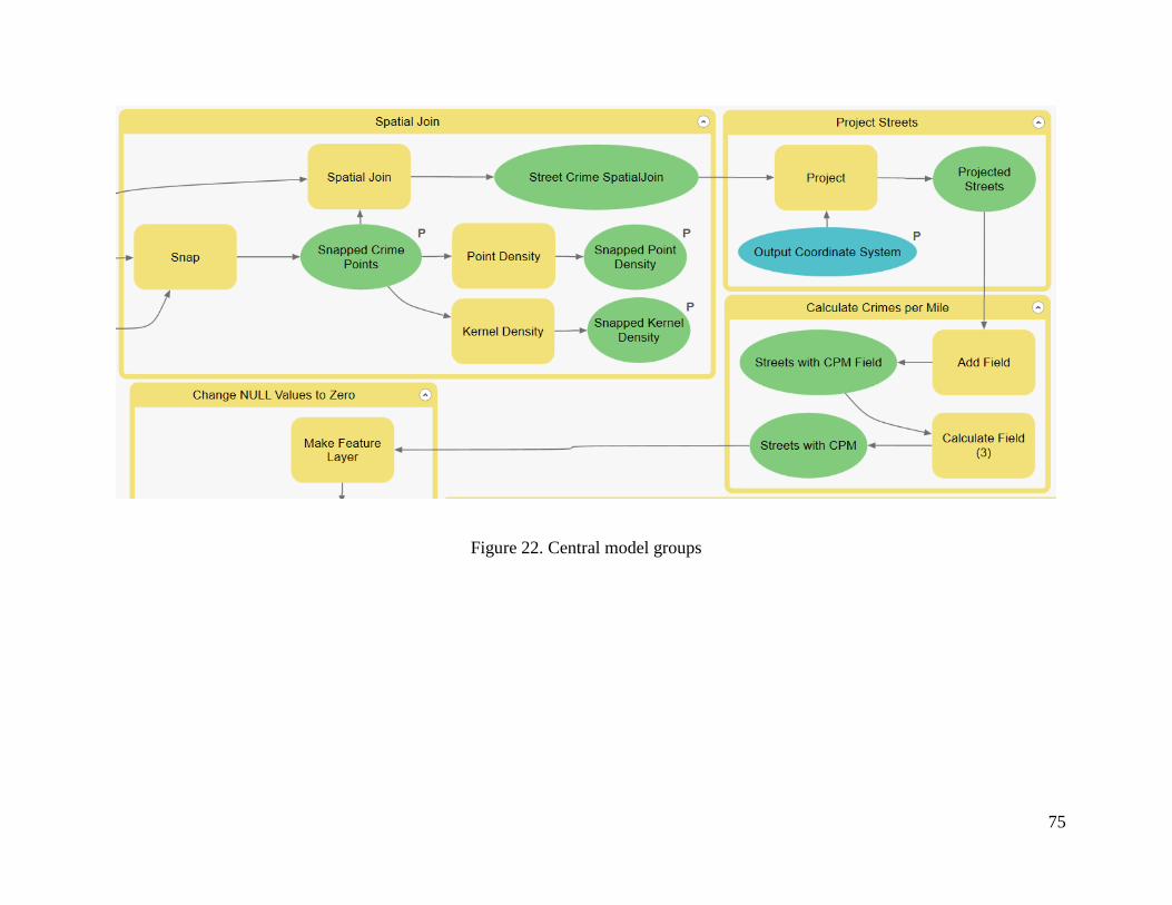
75

Figure 22. Central model groups

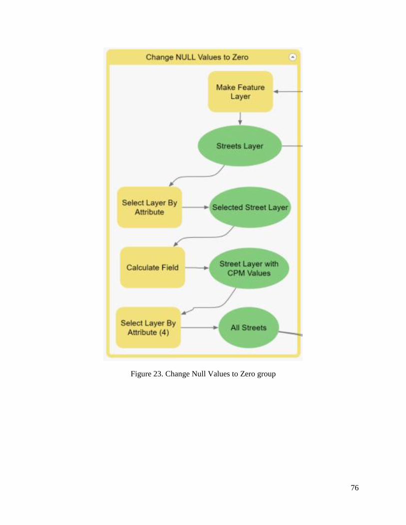
76

Figure 23. Change Null Values to Zero group

77

Figure 24. Generate Spatial Weight Matrix group

78

Figure 25. Spatial Statistics group