– Independent Work Report Fall, 2015 –

Creating Diversified Portfolios Using Cluster Analysis

Karina MarvinAdviser: Swati Bhatt

Abstract

Because of randomness in the market, as well as biases often seen in human behavior related to

investing and illogical decision making, creating and managing successful portfolios of financial

assets is a difficult practice. Achieving high returns with low risk is ideal, but seemingly impossible.

Modern portfolio theory states that diversification of assets is the most effective way to get low

risk-reward ratios [6]. However, how can one diversify effectively while at the same time avoiding

biases? The solution is an automated method of diversification using cluster analysis of financial

assets. The cluster analysis serves as a method to find which assets are different from each other

[15]. What is the best measure of difference or similarity between stocks? Previous works have

attemped to utilitze this type of algorithm using the correlation between stocks as the similarity

measure driving the clustering [11, 12]. However, correlations often change during periods of

financial stress [14]. This would cause the clusters to no longer be structurally sound, during a time

when risk is high. This paper proposes an alternative measure of similarity to avoid this risk: an

average of the two ratios: RevenuesAssets and Net Income

Assets . Therefore, companies with similar RevenuesAssets and

Net IncomeAssets ratios will be in the same cluster, while companies with varying Revenues

Assets and Net IncomeAssets

ratios will be in different clusters. Then, diversified portfolios of high performing stocks can be

created by picking assets with the highest Sharpe ratios from different clusters. Testing delays in

the financial statements that are used as well as weighting of the ratios, this algorithm results in

high performance portfolios, when compared to the S&P 500 from July 2000 to July 2015. This

is particularly true during the pre-crisis and post-crisis periods, 2000 to 2007 and 2009 to 2015

respectively. During the crisis period of 2007 to 2009, the algorithm portfolios do not perform as

well as they do in the other periods, however they still perform adequately compared to the S&P

500.

1. Introduction

Maintaining and managing a portfolio of investments is a much puzzled-over activity. There are

many issues that contribute to the confusion and difficulty of investing. Primarily, investors are

subject to a lot of uncertainty and randomness. There are even schools of thought and economic

theory that state it is not possible to beat the market using savvy stock selection or good timing. The

efficient market hypothesis is a theory that claims share prices of stocks always trade at fair value

because they incorporate all relevant information [5]. This hypothesis therefore implies that it is

impossible for one to sell stocks that are too inflated or buy stocks that are undervalued. Although

there is opposition to the efficient market hypothesis, the extreme availability of data in recent years

suggests that market prices more quickly reflect a value close to the true value of the stocks. This

implies that an investor cannot beat the market consistently because market prices will only change

in reaction to news, which by definition is random. An investor, therefore, can only obtain higher

returns by partaking in riskier investments.

Additionally, when one picks an asset to invest in, there are many different biases that affect

the investor. Illogical decision making has been observed in studies on human behavior when

financial choices are being made. For example, it has been shown that people tend to overweight

tail events, or events that are highly unlikely to happen, in their decision making [2]. This is why

many participate in lotteries, despite the miniscule chance of winning. Additionally, people tend to

have a negativity bias, or an overweighting of bad news than good news [13]. This causes investors

to be more cautious or risk averse about losses rather than gains, despite the fact that they should be

treated equally in economic analysis [13]. Due to these biases and the many more that influence

the decision-making of investors, a more quantitative and formulaic way to choose investments

is necessary to reduce biases in judgement, as well as reduce risk and maximize returns despite

uncertainty in the market.

Modern portfolio theory is the most widely used practice by individuals to develop portfolios.

It is based on a principle of attempting to maximize expected return for a given amount of risk or

2

equivalently minimizing risk for a given amount of return [6]. A highly utilized method to reduce

risk is diversification. The idea of diversification is to split investment between varying companies

so that if a few securities one owned were to take a downturn, the others would not, reducing the

loss. The downturn could be related to many factors, including the indsutry, market, country, type

of asset, or company itself.

Risk can be diversified by picking assets that are different from each other with respect a particular

aspect about the assets themselves. This aspect could be related to industry, country, type of asset,

or more. For example, two stocks in the same industry may move together. Additionally, two

European stocks may move together while an American stock moves differently. However, there are

an infinite number of ways that assets can be related and connected to one another that could result

in an issue for the investor in a crisis. There is no formulaic mechanism one can use to diversify

portfolios. Furthermore, the biases common in human behavior are still present and influential over

investment decisions. Therefore, an automated method to classify or cluster assets would be very

useful and essential to investment decision-making and the practice of diversification. The stocks

would be separated into groups via a clustering method that maximizes similarity within groups and

minimizes simiarity between groups. Doing this with securities would allow one to figure out what

combination of assets could make up a well diversified portfolio.

2. Background

2.1. 2008 Financial Crisis

The 2008 Financial Crisis, which is also known as the Global Financial Crisis, is thought to be the

worst and most severe crisis since the Great Depression in the 1930s. There were many causes

of the crisis, particularly the increase in subprime mortgages and mortgage-backed securities that

were only insured by credit default swaps. House prices rose steadily from the 1990s to 2006.

During this time, it was commonly thought that real estate was a safe and guaranteed successful

investment. As a result, home ownership increased to 68.6% of households by 2007 [1]. During this

time, mortgage lenders began to make subprime loans to people who usually would not be approved

3

for one. Banks securitized these loans through mortgage backed securities. The two biggest

issuers of these securities were Fannie Mae and Freddie Mac. When the housing market began

to plummet dramatically in 2006, the mortgage-backed securites became worthless as subprime

borrowers defaulted. Furthermore, personal wealth fell, reducing consumption and negatively

affecting businesses. It became very difficult to sell any suspicious assets, and the stock market

plummeted. Banks were further hurt by the lack of confidence, who began to withdraw all of

their money. When the Lehman Brothers went bankrupt in September 2008 due to large losses on

mortgage-backed securities, the panic in the markets multiplied. Governments and central banks

responded with large amounts of fiscal stimulus and institutional bailouts. There was an influx of

regulatory action and a slow recovery began. In June 2009, the financial crisis was declared to be

over, as the world continued to recover.

During the few years of the 2008 financial crisis, the stock markets were in complete turmoil.

In less than a month, from September 19, 2008 to October 10, 2008, the Dow Jones Industrial

Average plummeted 3600 points [1]. The S&P 500 fell 38.5% and the NASDAQ composite index

fell 40.5%, in 2008 alone [1]. These three are US market indices that are commonly followed and

are thought to be representative of the health of the American economy. The extreme financial

stress and systematic risk during this period affected investors and markets worldwide. While the

economy has improved greatly from 2008 to 2015, it is important to note that this period of financial

stress occurred, and could possibly occur again. Therefore, in order to accurately and effectively

stress test any investing algorithms or strategies, the 2007 to 2009 period must be used as a worst

case scenario test.

2.2. Diversification and the Financial Crisis

Diversification is the process of choosing investments in order to reduce exposure to any one

particular asset. This is typically done by investing in a variety of assets. If the asset prices do

not move together, then a diversified portfolio of those assets will have a lower variance than the

weighted average variance of the assets. The portfolio’s volatility could even be lower than any

4

single asset inside the portfolio.

Risk, which is defined as the chance that an investment’s return will be different than expected, is

what is trying to be reduced in diversification. There are two basic types of risk: systematic risk and

idiosyncratic risk. Systematic risk influences a large number of assets at once. It is inherent to the

entire market, not just a particular stock or industry [9]. Because of this, it is impossible to diversify

away systematic risk.

Idiosyncratic risk, on the other hand, only affects a small number of assets. This type of risk can

also be referred to as unsystematic risk or specific risk, because it typically will affect a specific

stock [9]. For example, news about a company such as a sudden strike will change the stock price

of that company, and possibly a couple competitors of the company. The risk of this occuring is

idiosyncratic risk, which one can protect themselves from using diversification.

The capital asset pricing model or the CAPM describes the relationship between risk and expected

return [10].

E[ra] = r f +βa(E[rm]− r f ) (1)

where E[ra] is the expected return on asset a, r f is the risk-free rate, βa is the beta of a, and E[rm]

is the expected return on the market. β is a measure of how much the security will respond to

swings in the market. In fact, it is a measure of the systematic risk of a security in comparison to

the market as a whole [10].

βa =σ2

amσ2

m(2)

where σ2am is the covariance between asset a and the market and σ2

m is the variance of the market.

If a regression is run between the return on the market and the return on an individual asset, the

following is achieved:

ra = αa +βarm + εa (3)

5

where εa is the error term, and measures the variability in ra that is independent of all other

securities in rm. Using this regression, the variance of a stock can be decomposed into its systematic

and idiosyncratic parts [10]:

σ2a = β

2a σ

2m +σ

2ε (4)

where σ2a is the total risk, β 2

a σ2m is the systematic risk, and σ2

ε is the idiosyncratic risk. This

idiosyncratic risk can be removed through diversification,

Portfolio variance is:

σ2(rp) =

n

∑i=1

n

∑j=1

wiw jσi j (5)

where σ2(rp) is the portfolio variance, n is the number of assets in the portfolio, wi is the portfolio

weight of an asset i, and σi j is the covariance of assets i and j, noting that the covariance of the

same asset is simply the variance of that asset. Therefore, lower covariance between assets can

greatly reduce the portfolio variance.

For very large n, portfolio variance becomes [10]:

σ2(rp) =

σ2

n+

n−1n

σ2i j (6)

where the first term is the average variance of the individual investments, the idiosyncratic risk,

and the second term is the average covariance, or the systematic risk. As n approaches infinity, the

first term approaches zero and the risk is diversified away.

However, the systematic risk remains. It will also be noted that there was a lot of systematic risk

during the 2008 financial crisis [9]. The economic event was certainly market-wide, with all types

of assets and securities decreasing in value due to the lack of confidence present. Diversification

can reduce risk to a large degree, but systematic risk cannot be removed.

6

2.3. Clustering Methods

Cluster analysis is the task of grouping a set of objects such that the objects within a group are

more similar to each other than the objects in other groups [15]. It is commonly used in statistical

data analysis. There are many algorithms designed to solve this task that differ in the definition

of a cluster and how the clusters are found. Typical problem parameters are similarity or distance

functions and the number of clusters.

Clustering methods can be divided into two basic types: hierarchical and partitional clustering.

Hierarchical clustering either merges smaller clusters into larger clusters or splits larger clusters into

smaller clusters [15]. This is typically used if the underlying structure behind the data is a tree and

is presented in a dendrogram. Partitional clustering, by contrast, directly partitions the data set into

a set of disjoint clusters [15]. The most commonly used partitional clustering method is k-means

clustering.

k-means clustering is a method of partitioning n observations into k clusters, in which each

observation belongs to the cluster with the nearest mean [15]. The goal is to minimize the within-

cluster sum of squares or:

argmins

k

∑i=1

∑x∈Si

||x−µi||2 (7)

where x are the obversations, S = S1,S2, ...,Sk are the sets of observations, and µi is the mean of

the points in Si. While this problem is NP-hard, there are commonly used heuristic algorithms, such

as Lloyd’s algorithm [15]. The algorithm employs an iterative refinement technique. It is initialized

by randomly assigning each observation to a cluster. Then, means are calculated to be the centroids

of the clusters in the update step. In the assignment step, each observation is assigned to the cluster

whose mean yields the least within-cluster sum of squares, where the sum of squares is the sum

of the squared Euclidean distance. Then, the new means are updated and the process continues

until convergence, when the assignment step no longer changes which cluster the observations are

assigned to. The process is shown graphically in the following Figure 1.

7

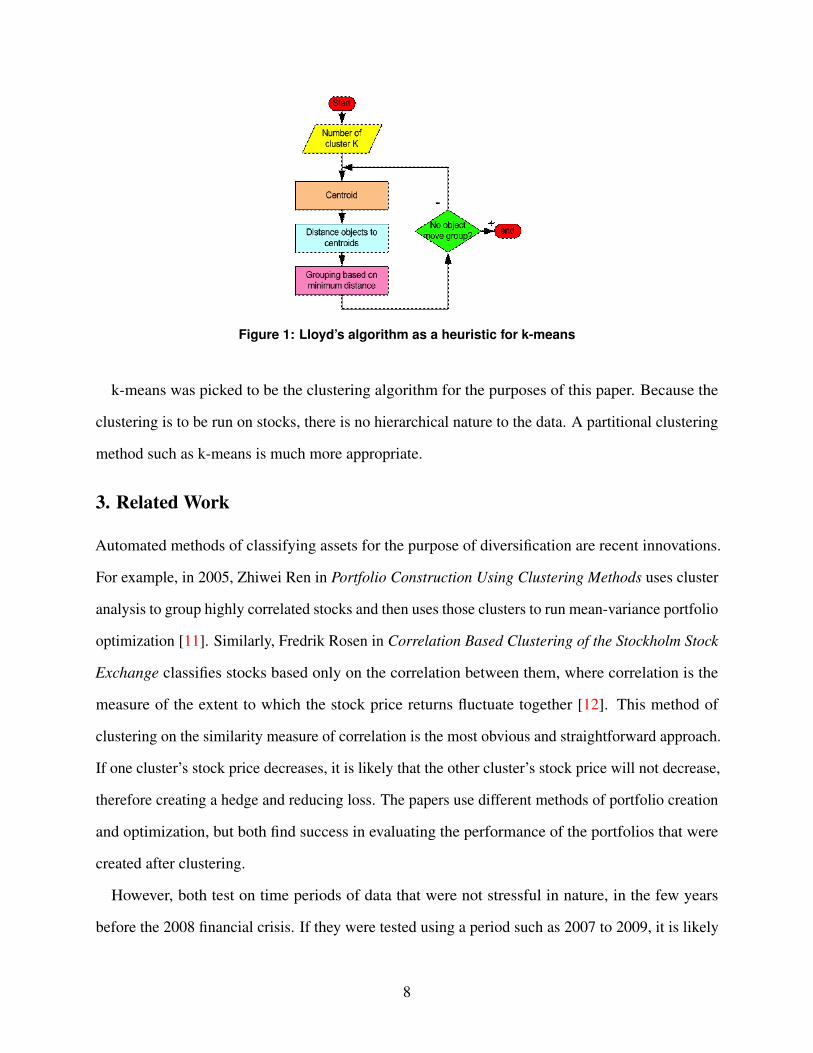
Figure 1: Lloyd’s algorithm as a heuristic for k-means

k-means was picked to be the clustering algorithm for the purposes of this paper. Because the

clustering is to be run on stocks, there is no hierarchical nature to the data. A partitional clustering

method such as k-means is much more appropriate.

3. Related Work

Automated methods of classifying assets for the purpose of diversification are recent innovations.

For example, in 2005, Zhiwei Ren in Portfolio Construction Using Clustering Methods uses cluster

analysis to group highly correlated stocks and then uses those clusters to run mean-variance portfolio

optimization [11]. Similarly, Fredrik Rosen in Correlation Based Clustering of the Stockholm Stock

Exchange classifies stocks based only on the correlation between them, where correlation is the

measure of the extent to which the stock price returns fluctuate together [12]. This method of

clustering on the similarity measure of correlation is the most obvious and straightforward approach.

If one cluster’s stock price decreases, it is likely that the other cluster’s stock price will not decrease,

therefore creating a hedge and reducing loss. The papers use different methods of portfolio creation

and optimization, but both find success in evaluating the performance of the portfolios that were

created after clustering.

However, both test on time periods of data that were not stressful in nature, in the few years

before the 2008 financial crisis. If they were tested using a period such as 2007 to 2009, it is likely

8

that the clusters would not remain structually sound. Correlations often reverse or change during

periods of stress [3]. Therefore the clusters that were formed based on correlations between stocks

would no longer be strongly positively correlated within the clusters and uncorrelated or strongly

negatively correlated between the clusters. This would mean the investor is no longer holding a

diversified portfolio, putting them at risk of large losses. Furthermore, the increased risk would be

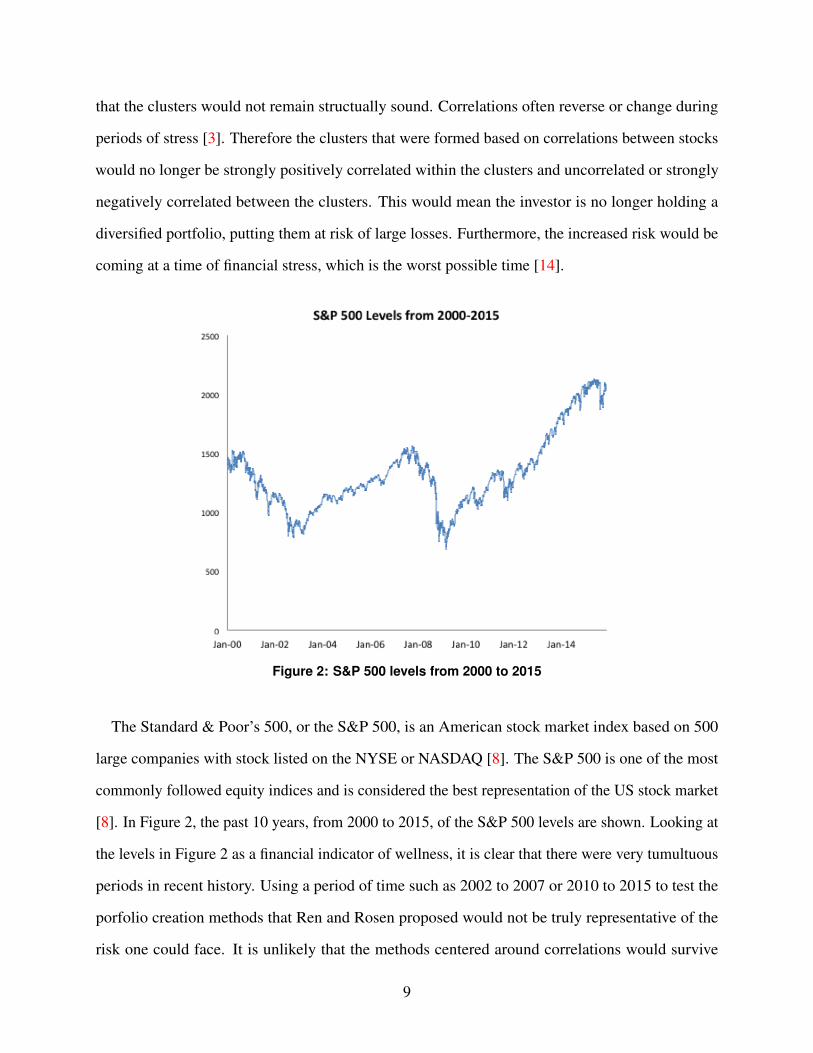
coming at a time of financial stress, which is the worst possible time [14].

Figure 2: S&P 500 levels from 2000 to 2015

The Standard & Poor’s 500, or the S&P 500, is an American stock market index based on 500

large companies with stock listed on the NYSE or NASDAQ [8]. The S&P 500 is one of the most

commonly followed equity indices and is considered the best representation of the US stock market

[8]. In Figure 2, the past 10 years, from 2000 to 2015, of the S&P 500 levels are shown. Looking at

the levels in Figure 2 as a financial indicator of wellness, it is clear that there were very tumultuous

periods in recent history. Using a period of time such as 2002 to 2007 or 2010 to 2015 to test the

porfolio creation methods that Ren and Rosen proposed would not be truly representative of the

risk one could face. It is unlikely that the methods centered around correlations would survive

9

during periods of fincicial distress, during which the stabilitiy of one’s investments is arguably most

important. The question is then: is there a safer measure than correlation to run the cluster analysis

on that results in portfolios that perform just as well?

4. Methodology

4.1. Clustering Measure of Similarity

Correlation as a measure of similarity does not hold up in periods of stress. A potential candidate

for a good measure of similarity would be related to the previous success or potential for growth of

the companies and be more inherent to the companies than correlation of stock prices. Then, the

structure of the clusters formed on the basis of the similarity measure would not crumble during

stressful time periods.

The measure of similarity proposed and evaluated in this paper is based on two financial ratios:

revenues to assets and net income to assets. A weighted average of these ratios is taken, and the

difference between the weighted averages of different firms serves as the similarity measurement.

Financial statements are released by all public firms every quarter. Revenue, net income and

assets are some of the measures that are present on these financial statments. Revenues, which

are on a company’s income statement, are the amount of money that a company receives during

a specific period, also known as sales [7]. Net income, by contrast, is a company’s total earnings

or profit. It is calculated by taking revenues and subtracting the cost of doing business including

cost of goods, interest, taxes, depreciation, and other expenses [7]. These two measures are often

considered when evaluating the strength or health of a business. They are thought to be the most

important figures on quarterly reports and are both evaluated because it is possible for net income to

increase while revenue remains the same, suggesting costs were cut. Revenue can indicate potential

for growth or success in the market, while net income is the actual profit the firm takes in. Both are

inherent to a company’s business every quarter and relate to the company’s performance over the

quarter.

However, a larger company is more likely to have high revenues and net income than a startup or

10

a small company. The sizes, however, do not necessarily correlate to worthiness in investment. In

order to scale for size, the revenues and net income values are divided by assets. Assets are also

released in finanical statements every quarter and are shown on the balance sheet of a corporation.

Generally, assets include cash, accounts receivable, inventory, real estate, and equipment [4]. This

measure is commonly used as a representation of size of company. Therefore, the revenues and net

income can be scaled by size by dividing by assets.

4.2. Portfolio Creation

Using the difference of weighted averages as a measure of similarity, a clustering method is run on

the data to partition it into groups. Then, a stock must be picked from each cluster. The clusters are

ideally very different from each other. Therefore, a portfolio containing a stock from each cluster

will be diversified. How should the stock from each cluster be picked? In the interest of having high

returns and low risks, stocks are picked to maximize the return to risk ratio. The Sharpe ratio, or the

average return earned in excess of the risk-free rate per unit of volatility, is a measure of calculating

risk-adjusted return. The stock from each cluster with the highest Sharpe ratio is therefore picked to

be in the portfolio. The portfolio is then diversified and comprised of historically high performing

stocks.

4.3. Variables

Multiple values were varied to determine the most successful combination in portfolio creation. The

weight of the revenues per asset ratio is varied from 0% to 100% in the weighted average used in

the similarity measure. The similarity measure is then:

RevenuesAssets

x+Net Income

Assets(1− x) (8)

where x ranges from 0 to 1. This measures any combination of the two ratios, including the pure

RevenuesAssets ratio and the pure Net Income

Assets ratio.

Additionally, a delay in effect from previous quarters of data is also varied. Three delay models

11

are investigated: one period, two period and average. A one period delay is simply using the most

recently published quarterly data to make a portfolio for the upcoming quarter. A two period delay

is using the financial data published the quarter before the most recent published data. In addition

to these two delays, the average delay model is using the average of the previous two quarters data

for the cluster analysis. These three methods are compared to see which is the most successful.

5. Implementation

668 stocks in the technology sector that are traded on the NYSE and NASDAQ were used for the

purpose of testing. Quarterly data on revenues, net income and assets, as well as daily data on stock

price returns, were found from 2000 to 2015. The companies that did not have data for this period

of time were removed, leaving 229 potential stocks to invest in. k-means clustering was run every

quarter to create portfolios.

5.1. Determination of k for k-means

In order to maximize viability of the clusters created, an appropriate value for k must be determined.

There is unlikely to be an obvious separation between clusters in the data; additionally, it would

be ideal to not have to visually determine the number of clusters every quarter. To determine the

appropriate k, two measures were considered: the ratio of between cluster sum of squares to total

sum of squares, as well as silhouette width.

The between cluster sum of squares is the sum of the squared Euclidean distance between every

observation and the mean of all of the clusters it does not belong to [15]. The within-cluster sum of

squares, by contrast, is the sum of the squared Euclidean distance between every observation and

the mean of the cluster it belongs to. The total sum of squares is the sum of the two. Therefore, the

ratio of between sum of squares to total sum of squares measures what percentage of the variance

in the clustering is between clusters. Intuitively, between cluster sum of squares to total sum of

squares is the amount of variance in the data that is accounted for between clusters, rather than

within clusters.

Sihouette widths are a common measure of consistency of clusters [15]. For each point p, the

12

average distance between that point and all other points within the cluster is calculated, as well

as the average distance between p and all points in the nearest cluster. The silhouette width is the

difference between these two divided by the greater of the two. If there is strong cohesion within a

group and weak cohesion between groups, the coefficients will be high.

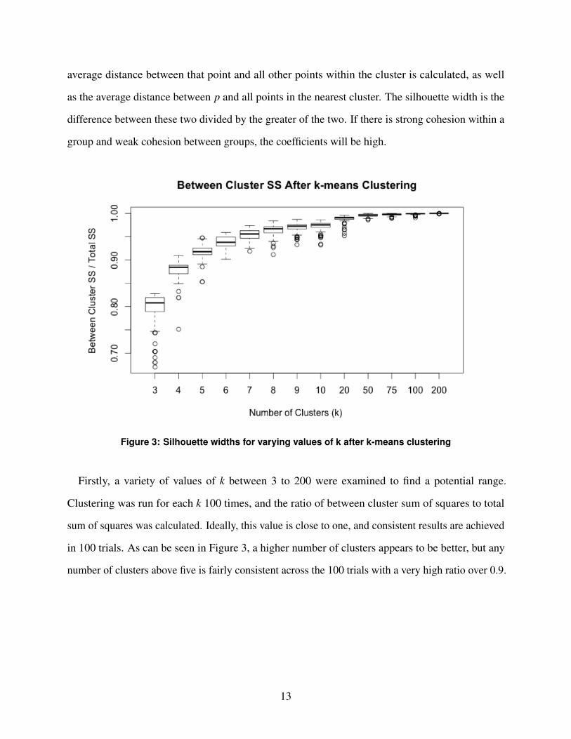
Figure 3: Silhouette widths for varying values of k after k-means clustering

Firstly, a variety of values of k between 3 to 200 were examined to find a potential range.

Clustering was run for each k 100 times, and the ratio of between cluster sum of squares to total

sum of squares was calculated. Ideally, this value is close to one, and consistent results are achieved

in 100 trials. As can be seen in Figure 3, a higher number of clusters appears to be better, but any

number of clusters above five is fairly consistent across the 100 trials with a very high ratio over 0.9.

13

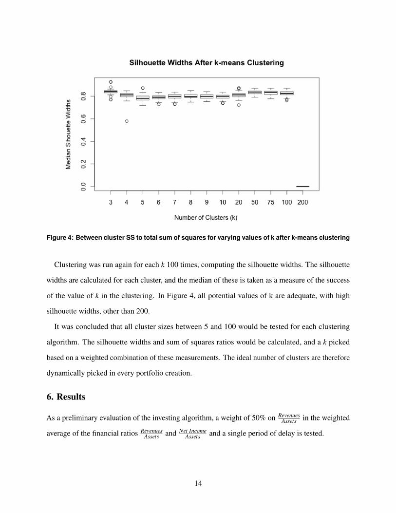
Figure 4: Between cluster SS to total sum of squares for varying values of k after k-means clustering

Clustering was run again for each k 100 times, computing the silhouette widths. The silhouette

widths are calculated for each cluster, and the median of these is taken as a measure of the success

of the value of k in the clustering. In Figure 4, all potential values of k are adequate, with high

silhouette widths, other than 200.

It was concluded that all cluster sizes between 5 and 100 would be tested for each clustering

algorithm. The silhouette widths and sum of squares ratios would be calculated, and a k picked

based on a weighted combination of these measurements. The ideal number of clusters are therefore

dynamically picked in every portfolio creation.

6. Results

As a preliminary evaluation of the investing algorithm, a weight of 50% on RevenuesAssets in the weighted

average of the financial ratios RevenuesAssets and Net Income

Assets and a single period of delay is tested.

14

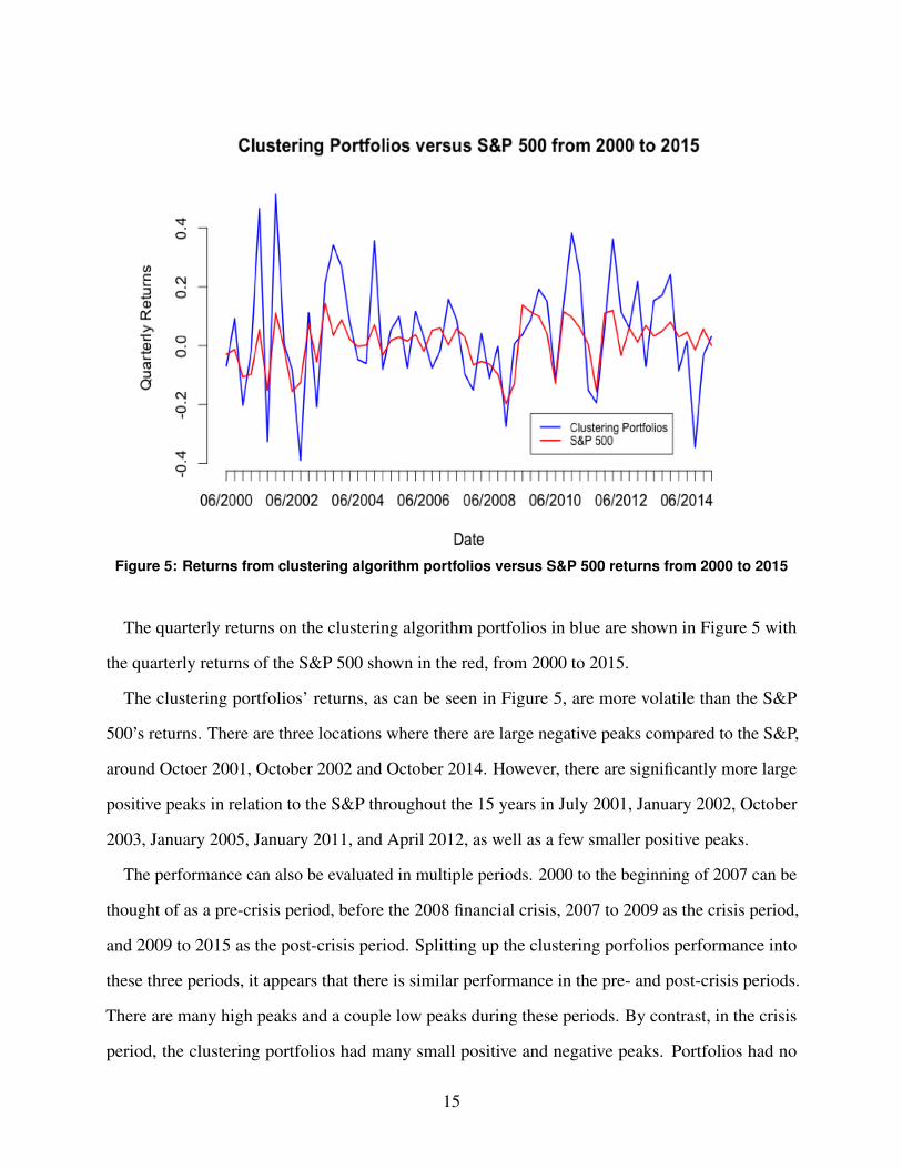
Figure 5: Returns from clustering algorithm portfolios versus S&P 500 returns from 2000 to 2015

The quarterly returns on the clustering algorithm portfolios in blue are shown in Figure 5 with

the quarterly returns of the S&P 500 shown in the red, from 2000 to 2015.

The clustering portfolios’ returns, as can be seen in Figure 5, are more volatile than the S&P

500’s returns. There are three locations where there are large negative peaks compared to the S&P,

around Octoer 2001, October 2002 and October 2014. However, there are significantly more large

positive peaks in relation to the S&P throughout the 15 years in July 2001, January 2002, October

2003, January 2005, January 2011, and April 2012, as well as a few smaller positive peaks.

The performance can also be evaluated in multiple periods. 2000 to the beginning of 2007 can be

thought of as a pre-crisis period, before the 2008 financial crisis, 2007 to 2009 as the crisis period,

and 2009 to 2015 as the post-crisis period. Splitting up the clustering porfolios performance into

these three periods, it appears that there is similar performance in the pre- and post-crisis periods.

There are many high peaks and a couple low peaks during these periods. By contrast, in the crisis

period, the clustering portfolios had many small positive and negative peaks. Portfolios had no

15

large peaks during this period, on the positive or negative side. The algorithm portfolios are less

volatile during the crisis period, due to the systematic risk across all markets during the period. The

conservative natrue of the investments during this period compared to the other periods is a good

feature of the algorithm.

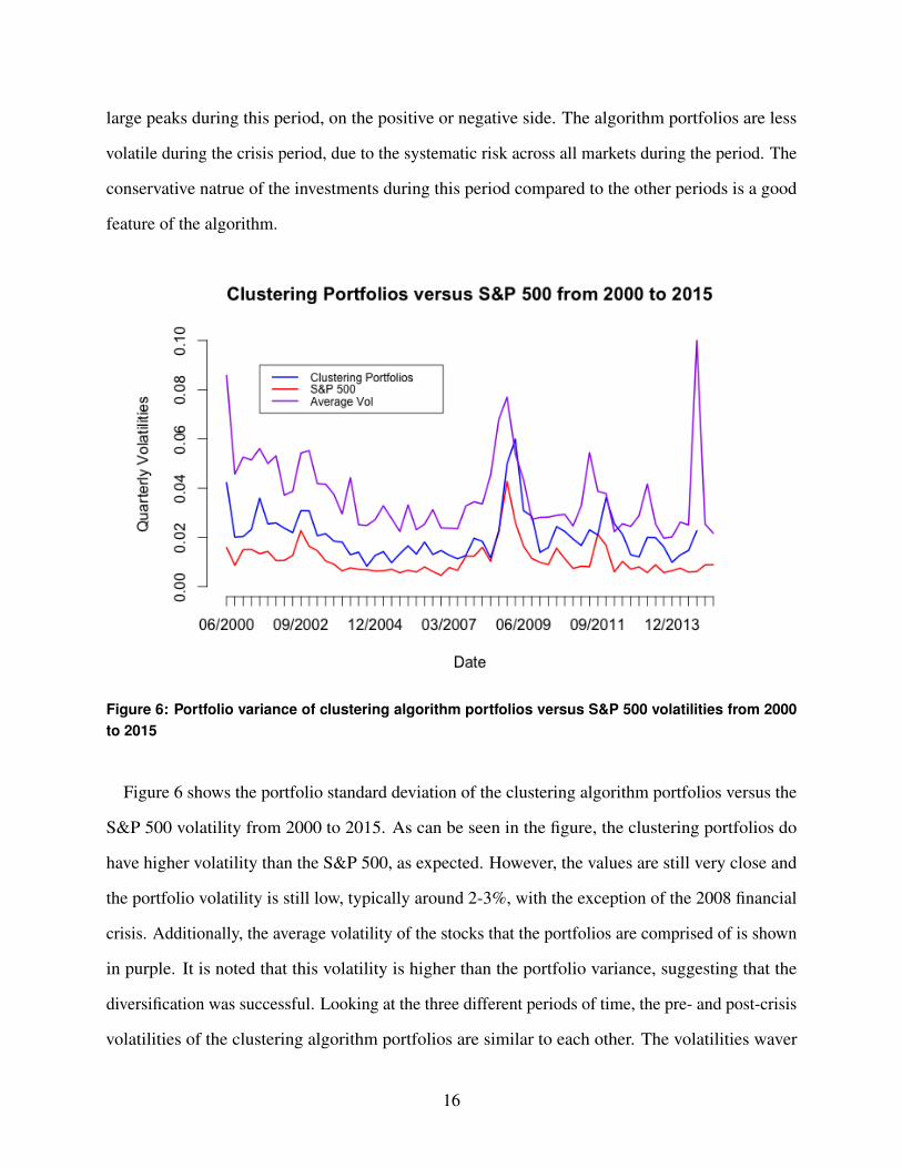
Figure 6: Portfolio variance of clustering algorithm portfolios versus S&P 500 volatilities from 2000to 2015

Figure 6 shows the portfolio standard deviation of the clustering algorithm portfolios versus the

S&P 500 volatility from 2000 to 2015. As can be seen in the figure, the clustering portfolios do

have higher volatility than the S&P 500, as expected. However, the values are still very close and

the portfolio volatility is still low, typically around 2-3%, with the exception of the 2008 financial

crisis. Additionally, the average volatility of the stocks that the portfolios are comprised of is shown

in purple. It is noted that this volatility is higher than the portfolio variance, suggesting that the

diversification was successful. Looking at the three different periods of time, the pre- and post-crisis

volatilities of the clustering algorithm portfolios are similar to each other. The volatilities waver

16

between 1 and 3 percent, following a similar pattern to the S&P 500 volatilies’ movements. In

the crisis period, volatility spikes to around 6%. During this time, the S&P 500 volatility also

spikes, although to a lower value. Because the 2008 financial crisis caused high systematic risk,

the portfolio volatility is expected to increase greatly. Overall, the volatility of the portfolios is

greater than ideal, but is still low enough to be acceptable and is representative of the underlying

diversification.

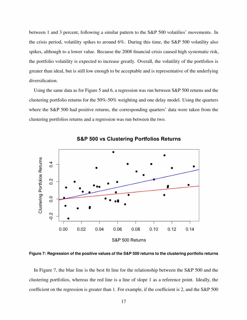
Using the same data as for Figure 5 and 6, a regression was run between S&P 500 returns and the

clustering portfolio returns for the 50%-50% weighting and one delay model. Using the quarters

where the S&P 500 had positive returns, the corresponding quarters’ data were taken from the

clustering portfolios returns and a regression was run between the two.

Figure 7: Regression of the positive values of the S&P 500 returns to the clustering portfolio returns

In Figure 7, the blue line is the best fit line for the relationship between the S&P 500 and the

clustering portfolios, whereas the red line is a line of slope 1 as a reference point. Ideally, the

coefficient on the regression is greater than 1. For example, if the coefficient is 2, and the S&P 500

17

returned 10% in one quarter, it would be estimated that the portfolios would return 20%. As can be

seen in Figure 7, the coefficient is significantly above 1, at just below 2. In fact, a return on the S&P

of 15% is estimated to correlate with a return of around 30% on the clustering algorithm portfolios.

However, it is noted that there is a decent amount of variation around this regression, as can be seen

by the points in Figure 7 and the R2 value from the regression of 0.32.

In order to determine if the coefficient is significantly different from 1, the same regression is run

with an offset of the S&P 500 returns, where the offset is subtracted from the response variable to

test the null hypothesis β = 1 in the equation:

PR[posIndices] = α +SNPR[posIndices]β (9)

where PR[posIndices] is the portfolio returns at the indicies where the S&P 500 is positive,

SNPR[posIndices], is the S&P 500 returns where they are positive, and α and β are the coefficients

of the regression. The regression results in a p-value of 0.0319 on β , so the null hypothesis is

rejected at 95% confidence. It is accepted that the coefficient β is significantly greater than 1.

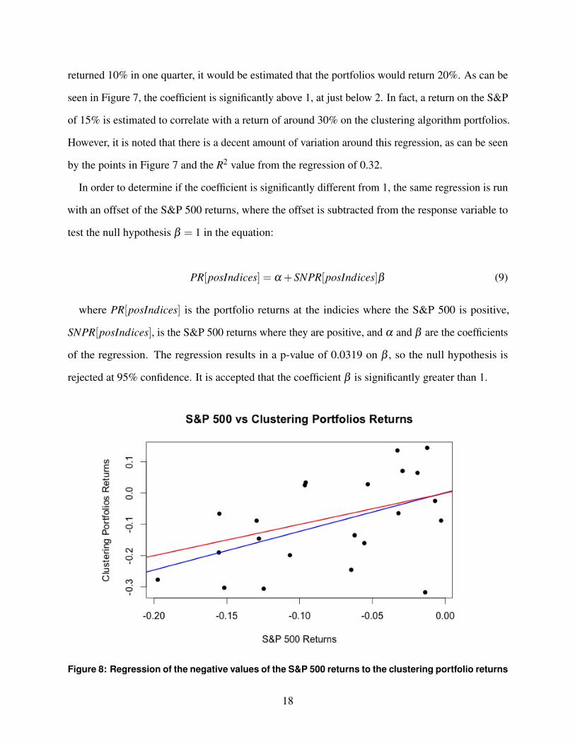
Figure 8: Regression of the negative values of the S&P 500 returns to the clustering portfolio returns

18

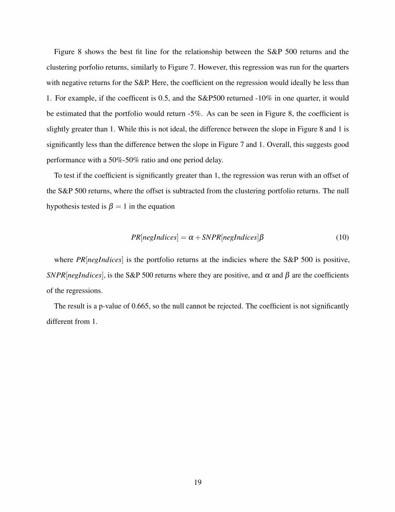
Figure 8 shows the best fit line for the relationship between the S&P 500 returns and the

clustering porfolio returns, similarly to Figure 7. However, this regression was run for the quarters

with negative returns for the S&P. Here, the coefficient on the regression would ideally be less than

1. For example, if the coefficent is 0.5, and the S&P500 returned -10% in one quarter, it would

be estimated that the portfolio would return -5%. As can be seen in Figure 8, the coefficient is

slightly greater than 1. While this is not ideal, the difference between the slope in Figure 8 and 1 is

significantly less than the difference betwen the slope in Figure 7 and 1. Overall, this suggests good

performance with a 50%-50% ratio and one period delay.

To test if the coefficient is significantly greater than 1, the regression was rerun with an offset of

the S&P 500 returns, where the offset is subtracted from the clustering portfolio returns. The null

hypothesis tested is β = 1 in the equation

PR[negIndices] = α +SNPR[negIndices]β (10)

where PR[negIndices] is the portfolio returns at the indicies where the S&P 500 is positive,

SNPR[negIndices], is the S&P 500 returns where they are positive, and α and β are the coefficients

of the regressions.

The result is a p-value of 0.665, so the null cannot be rejected. The coefficient is not significantly

different from 1.

19

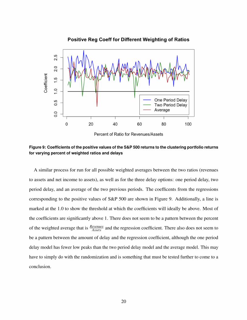
Figure 9: Coefficients of the positive values of the S&P 500 returns to the clustering portfolio returnsfor varying percent of weighted ratios and delays

A similar process for run for all possible weighted averages between the two ratios (revenues

to assets and net income to assets), as well as for the three delay options: one period delay, two

period delay, and an average of the two previous periods. The coefficents from the regressions

corresponding to the positive values of S&P 500 are shown in Figure 9. Additionally, a line is

marked at the 1.0 to show the threshold at which the coefficients will ideally be above. Most of

the coefficients are significantly above 1. There does not seem to be a pattern between the percent

of the weighted average that is RevenuesAssets and the regression coefficient. There also does not seem to

be a pattern between the amount of delay and the regression coefficient, although the one period

delay model has fewer low peaks than the two period delay model and the average model. This may

have to simply do with the randomization and is something that must be tested further to come to a

conclusion.

20

Figure 10: Coefficients of the negative values of the S&P 500 returns to the clustering portfolioreturns for varying percent of weighted ratios and delays

The same process was run for the negative S&P 500 returns, all possible weighted averages of

the financial ratios, and the three delay models. The results in Figure 10 show that the coefficients

are fairly consistent over the delay periods as well as the weights of the ratios. The coefficients are

above 1, as seen earlier, however, they are only slightly above, versus being significantly above

1 in the positive range of S&P values. While the coefficients are not in the ideal range, they are

acceptable, particularly in comparison to the positive part of the regression.

6.1. An Example of Investment

To provide an idea of what kind of earnings would have been achieved using the clustering algorithm

to create portfolios, a concrete example of investment is explored here. In the following example, a

50%-50% weighting of the two financial ratios is used.

Assuming an initial investment of 1000 dollars in July 2000 and the reinvestment of all money

that was returned from the investment every quarter, Table 1 shows the final amount of money the

21

investor earns.

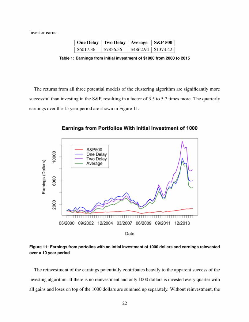
One Delay Two Delay Average S&P 500$6017.36 $7856.56 $4862.94 $1374.42

Table 1: Earnings from initial investment of $1000 from 2000 to 2015

The returns from all three potential models of the clustering algorithm are significantly more

successful than investing in the S&P, resulting in a factor of 3.5 to 5.7 times more. The quarterly

earnings over the 15 year period are shown in Figure 11.

Figure 11: Earnings from porfolios with an intial investment of 1000 dollars and earnings reinvestedover a 10 year period

The reinvestment of the earnings potentially contributes heavily to the apparent success of the

investing algorithm. If there is no reinvestment and only 1000 dollars is invested every quarter with

all gains and loses on top of the 1000 dollars are summed up separately. Without reinvestment, the

22

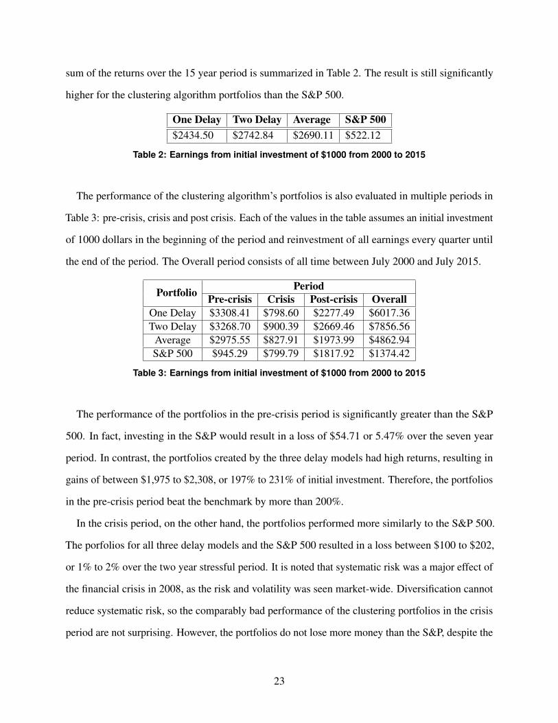
sum of the returns over the 15 year period is summarized in Table 2. The result is still significantly

higher for the clustering algorithm portfolios than the S&P 500.

One Delay Two Delay Average S&P 500$2434.50 $2742.84 $2690.11 $522.12

Table 2: Earnings from initial investment of $1000 from 2000 to 2015

The performance of the clustering algorithm’s portfolios is also evaluated in multiple periods in

Table 3: pre-crisis, crisis and post crisis. Each of the values in the table assumes an initial investment

of 1000 dollars in the beginning of the period and reinvestment of all earnings every quarter until

the end of the period. The Overall period consists of all time between July 2000 and July 2015.

Portfolio PeriodPre-crisis Crisis Post-crisis Overall

One Delay $3308.41 $798.60 $2277.49 $6017.36Two Delay $3268.70 $900.39 $2669.46 $7856.56

Average $2975.55 $827.91 $1973.99 $4862.94S&P 500 $945.29 $799.79 $1817.92 $1374.42

Table 3: Earnings from initial investment of $1000 from 2000 to 2015

The performance of the portfolios in the pre-crisis period is significantly greater than the S&P

500. In fact, investing in the S&P would result in a loss of $54.71 or 5.47% over the seven year

period. In contrast, the portfolios created by the three delay models had high returns, resulting in

gains of between $1,975 to $2,308, or 197% to 231% of initial investment. Therefore, the portfolios

in the pre-crisis period beat the benchmark by more than 200%.

In the crisis period, on the other hand, the portfolios performed more similarly to the S&P 500.

The porfolios for all three delay models and the S&P 500 resulted in a loss between $100 to $202,

or 1% to 2% over the two year stressful period. It is noted that systematic risk was a major effect of

the financial crisis in 2008, as the risk and volatility was seen market-wide. Diversification cannot

reduce systematic risk, so the comparably bad performance of the clustering portfolios in the crisis

period are not surprising. However, the portfolios do not lose more money than the S&P, despite the

23

increased volatility in comparison. Taking this into consideration, the performance of the clustering

portfolios during the crisis period is adequate.

The post crisis period had high returns for all delay models and the S&P 500. Investing in the

S&P 500 returned $817.92 or 81.7%. The other portfolios had returned between $974 and $1669

or 97% to 167%. While the difference between these returns and the S&P is smaller than for the

pre-crisis period, the clustering portfolios still perform significantly better than the S&P during this

period.

7. Conclusion

Diversified portfolios reduce idiosyncratic risk, allowing an investor to increase returns without

drastically increasing risk. However, there is no widely accepted formulaic way to diversify

portfolios. There are infinitely many potential ways to diversify. Furthermore, actively managing

such a portfolio without falling to the effects of biases in human behavior is a time-consuming and

difficult task.

Machine learning and statistical data analysis has increasingly been utilized in the practice of

investing, in an effort to reduce the influence of biases as well as the amount of effort that is required

by managing a portfolio. A method that has recently been utilized for investing is cluster analysis,

or the grouping of data into clusters that are similar intra-cluster and different inter-cluster. While

this analysis sounds sufficient to assist with diversification, what defines similarity between stocks

or publicly traded companies?

The simplest approach to similarity is defined by movements in stock prices. High correlation

between stock prices would suggest similarity. Furthermore, investing in stocks that are uncorrelated

or negatively correlated with each other would be a direct hedge and would reduce risk in portfolios

[11, 12]. However, correlations between stocks are heavily reliant on the period that they are

calculated. In fact, during stressful time periods, correlations between stocks often change [3].

This would put the investor at risk of large losses during a time of high financial stress or the most

important time to be invested in safe portfolios.

24

The proposed alternative to correlation as a measure of similarity in this paper was the average

of two financial ratios: RevenuesAssets and Net Income

Assets . Due to the fact that these financial ratios are more

inherent to the future success or growth of a company than daily movements in stock prices, the

above proposal seemed logical.

In order to test the value of the two financial ratios in determining successful diversified portfolios,

portfolios were created for 60 quarters between 2000 and 2015. The two ratios were used for the

similarity measure in k-means clustering and stocks with high Sharpe ratios were picked from each

cluster to form the portfolios.

Furthermore, the appropriate weighting of the two tested financial ratios was tested, in addition to

varying levels of delay in data usage for the cluster analysis. All results were compared against the

S&P 500 from 2000 to 2015. The time period, which encompassed a variety of different levels of

financial stress, would serve as a reliable reflection of how the proposed algorithm would function.

The three delay models and the weighting of the financial ratios did not have a conclusive effect

on the performance of the clustering algorithm produced portfolios. In all cases, the portfolios

performed significantly better than the benchmark portfolio, the S&P 500. While the portfolios

were more volatile than the S&P, they were shown to be well diversified and held up during even

the arguably most stressful time period in recent history: the 2008 financial crisis.

Further work that could be done relating to this algorithm is testing on holding the diversified

portfolios for longer periods of time. The length used in this paper was one quarter; however, it is

possible that the portfolios could perform better if held for in two quarters, one year, or two years.

Furthermore, the algorithm could be tested on a different population of stocks. This paper looked at

668 stocks in the technology sector, which were then reduced to 229 due to the lack of available

data. Stocks in a different sector or the general population of stocks could be tested in addition.

This paper represents my own work in accordance with University regulations.

Karina Marvin

25

References[1] K. Amadeo, “2008 financial crisis: Causes, costs and could it reoccur?” About News, 2011.[2] N. Barberis, “The psychology of tail events: Progress and challenges,” American Economic Review, 2013.[3] N. Frank, “Linkages between asset classes during the financial crisis, accounting for market microstructure noise

and non-synchronous trading,” University of Oxford, 2009.[4] Investopedia. (2015) Assets.[5] Investopedia. (2015) Efficient market hypothesis.[6] Investopedia. (2015) Modern portfolio theory.[7] Investopedia. (2015) Revenue.[8] Investopedia. (2015) Standard & poor’s 500 index - s&p 500.[9] Investopedia. (2015) Systematic risk.

[10] P. Lynch, “Portfolio theory: The risk and return relationship,” ACCA Qualificiation, may 2004.[11] Z. Ren, “Portfolio construction using clustering methods,” Worcester Polytechnic Insitute, 2005.[12] F. Rosen, “Correlation based clustering of the stockholm stock exchange,” Stockhom University, 2006.[13] P. Rozin, “Negativity bias, negativity dominance, and contagion,” Personality and Social Psychology Review,

vol. 5, no. 4, pp. 296–320, 2001.[14] R. Scott-Ram, “Managing portfolio risk for periods of stress,” World Gold Council, dec 2000.[15] P.-N. Tan, Introduction to Data Mining. Pearson, 2006.

26