Banks international asset portfolios: optimality, linkages ... · Banks international asset portfolios: optimality, ... 4 Banks International Asset Portfolios: Optimality, Linkages

Eighth IFC Conference on “Statistical implications of the new financial landscape”

Basel, 8–9 September 2016

Banks international asset portfolios: optimality, linkages and resilience1

João Amador and João Falcão Silva, Bank of Portugal

1 This paper was prepared for the meeting. The views expressed are those of the authors and do not necessarily reflect the views of the BIS, the IFC or the central banks and other institutions represented at the meeting.

Banks International Asset Portfolios: Optimality, Linkages and Resilience 1

Banks International Asset Portfolios: Optimality, Linkages and Resilience

João Amador; João Falcão Silva

Abstract

The world economy has been living under the shadow of the latest global financial crisis. The persistence of high indebtedness levels across the world maintains these concerns on the agenda of economic institutions. This paper tries to address two main questions. First, it examines the cross country asset portfolios and uses network theory to map linkages between banking systems and discuss its resilience to shocks. Second, it assesses how distant are portfolios from an optimal diversification strategy.

Keywords: Banks, Cross-Border Asset Portfolio, Networks

JEL classification: F65, G15, G21

2 Banks International Asset Portfolios: Optimality, Linkages and Resilience

Introduction

Over the last decades, financial markets became more integrated and the size of cross-border portfolios increased significantly. Although the size of cross-border portfolios are strongly affected by valuation effects, international financial integration has deepened. This has been facilitated by higher liberalization of capital movements, as well as by technological progress in the communication and information industries. Nevertheless, many investors still do not seem to fully diversify their external portfolio assets, which are highly concentrated in a few non-resident countries. The high financial integration and the concentration of portfolios in few non-resident countries contributes to propagate and amplify the impact of crisis in specific economies, thus giving rise to aggregate shocks. The role of bank’s portfolios is particularly important in this respect because the systemic linkages are stronger and potentially disruptive.

The literature on the propagation of financial crisis has expanded in the recent years and it is too broad to be mentioned here. On the bank dimension recent examples are Bremus and Fratzscher (2014). These authors argue that cross-border bank lending has decreased and the home bias in the credit portfolio of banks has risen in the euro area. Their results suggest that expansionary monetary policy has encouraged cross-border lending, both in euro area and non-euro area countries. In addition, improvements in regulatory policy and increases in financial supervisory power have contributed to higher cross-border lending. Papers that assess banks’ international capital flows in the period of the financial crisis with view on financial stability are Hills and Hoggarth (2013) and Hoggarth, et al. (2010). In addition, in its 2012 report, the Committee on International Economic Policy and Reform (2012) signals that the procyclicality inherent in capital flows is not adequately addressed and makes a point for reinforced policy coordination. The literature on financial networks has also greatly expanded. For example, Joseph et al. (2014) analyse the network of cross-border equity and long-term debt securities portfolio investment and measure the robustness of the global financial system and the interdependence of financial markets. Finally, a paper that is important for the purpose of our study is that of Buch et al (2010). The aim of this paper is to identify optimal international asset portfolios for banks by using the mean–variance portfolio model with currency hedging. The benchmark portfolios are compared with the actual cross-border asset positions of banks from 1995 to 2003. Differences between the two portfolios are explained by some additional factors as regulations, institutions, cultural conditions / other financial frictions. In this article we focus on the representation of the bank’s international portfolio in a network setup. In this context the main cross-country portfolio linkages are represented as a directed and unweighted network, complemented by some basic measures that describe its topology and allow for a basic assessment of resilience. In addition, we operate a simple conceptual exercise where the existing portfolios are compared to those that emerge from an optimal allocation strategy. This article is organised as follows. Section 2 briefly describes the international banking statistics database used. In section 3, the banks’ international portfolios are described in December 2007 and March 2016 (the last available period), corresponding to the situation before the international financial and economic crisis and the present moment and their linkages are presented. Section 4 uses optimal portfolio theory to obtain the alternative banks’ international assets allocation and


discusses deviations relatively to the portfolio actually observed. Finally, section 5 presents some concluding remarks.

Data sources and description

International Banking Statistics

Data on International Banking statistics is disseminated by Bank for International Settlements which is composed by two datasets - Locational Banking Statistics (LBS) and Consolidated Banking Statistics (CBS). These two datasets refer to the international holdings of assets by banks at a country level from a set of reporting countries. However, they address different aspects of international banking activity. LBS data are a key source of information on the currency and geographical composition of resident banks’ balance sheets while CBS provides information about banking systems’ risk exposures, in particular country risk. CBS measures worldwide consolidated claims of banks headquartered in reporting countries, including claims of their own foreign affiliates but excluding inter-office positions.

Locational Banking Statistics

According to the BIS definition, Locational Banking Statistics are designed mainly to capture financial claims and liabilities of internationally active banks (i.e excluding only resident domestic banks without positions vis-à-vis non-residents of the reporting country). The statistics cover all on balance sheet positions and some off-balance sheet positions in the area of trustee business. The reporting basis underlying the statistics is the residence of the reporting banking office (conforms to balance of payments and international investment position statistics). These offices report exclusively their own (unconsolidated) business, including their international transactions with any of their own affiliates (branches, subsidiaries, joint ventures), including claims and liabilities vis-à-vis non-residents in any currency, claims and liabilities vis-à-vis residents of the reporting country in local currency as well as in foreign currencies. The Locational Banking Statistics comprise two subsets - locational banking statistics by residence (LBS/R) and locational banking statistics by nationality. The first subset combines the breakdown by residence of the reporting bank with a full country breakdown of counterparties, whereas the latter shows a breakdown by nationality of the reporting bank. Locational banking statistics by residence were considered for the purpose of this paper. The underlying assumption is that residence is a better proxy to capture shocks taking place in specific locations. Nevertheless, the results will are qualitatively unaltered with LBS by Nationality. The database covers the time period between 2004 and the first quarter of 2016 and is provided by the Bank for International Settlements (BIS) and similar to the published by the BIS in its Quarterly Review, but more detailed (with respect to bilateral asset positions).It comprises bilateral quarterly asset outstanding amounts for all instruments (Loans and deposits, debt securities and other assets and


liabilities), counterparty institutional sectors (Banks, General Government, Households and NPISHs, Nonbank financial institutions, Non-financial corporations) denominated in all currencies, with respect to non-resident counterparty countries located in each of the recipient countries1. Locational banking statistics are not consolidated which means that the claims of foreign subsidiaries of reporting banks are not included2. A sample of twenty one countries was considered to perform this analysis: Australia, Austria, Belgium, Brazil, Canada, Denmark, Finland, France, Germany, Greece, Italy, Ireland, Japan, Luxembourg, Netherlands, Portugal, Spain, Sweden, Switzerland, United Kingdom and United States. For these reporting countries foreign financial claims of banks located in the territory vis-à-vis counterparty country is available, and also information of foreign financial claims of banks located in other countries vis-à-vis these reporting countries.

Mapping the network of cross-border portfolios

Bilateral portfolios

Banks bilateral cross-border asset positions are defined as bank claims against non-resident countries located in each of the countries in the sample.

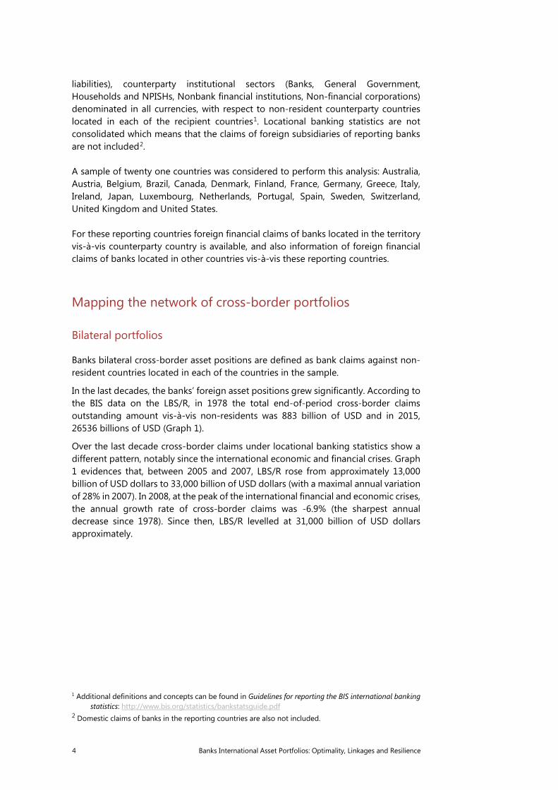
In the last decades, the banks’ foreign asset positions grew significantly. According to the BIS data on the LBS/R, in 1978 the total end-of-period cross-border claims outstanding amount vis-à-vis non-residents was 883 billion of USD and in 2015, 26536 billions of USD (Graph 1).

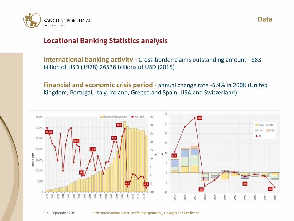
Over the last decade cross-border claims under locational banking statistics show a different pattern, notably since the international economic and financial crises. Graph 1 evidences that, between 2005 and 2007, LBS/R rose from approximately 13,000 billion of USD dollars to 33,000 billion of USD dollars (with a maximal annual variation of 28% in 2007). In 2008, at the peak of the international financial and economic crises, the annual growth rate of cross-border claims was -6.9% (the sharpest annual decrease since 1978). Since then, LBS/R levelled at 31,000 billion of USD dollars approximately.

1 Additional definitions and concepts can be found in Guidelines for reporting the BIS international banking

statistics: http://www.bis.org/statistics/bankstatsguide.pdf 2 Domestic claims of banks in the reporting countries are also not included.

http://www.bis.org/statistics/bankstatsguide.pdf


Graph 1 - Cross-border claims and annual growth

Source: BIS statistics.

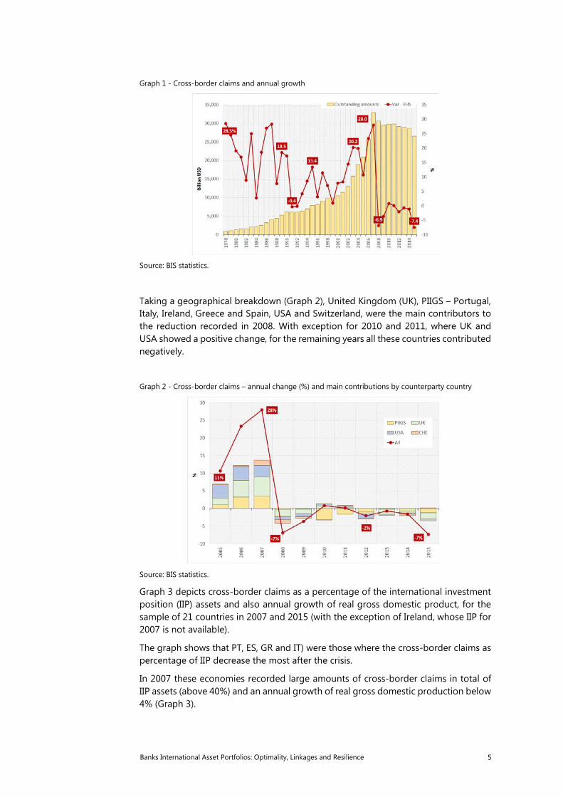
Taking a geographical breakdown (Graph 2), United Kingdom (UK), PIIGS – Portugal, Italy, Ireland, Greece and Spain, USA and Switzerland, were the main contributors to the reduction recorded in 2008. With exception for 2010 and 2011, where UK and USA showed a positive change, for the remaining years all these countries contributed negatively.

Graph 2 - Cross-border claims – annual change (%) and main contributions by counterparty country


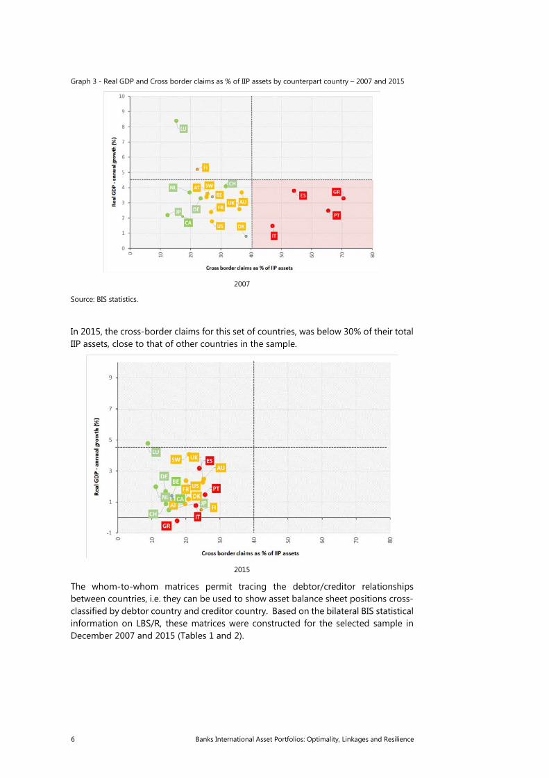
Graph 3 depicts cross-border claims as a percentage of the international investment position (IIP) assets and also annual growth of real gross domestic product, for the sample of 21 countries in 2007 and 2015 (with the exception of Ireland, whose IIP for 2007 is not available).

The graph shows that PT, ES, GR and IT) were those where the cross-border claims as percentage of IIP decrease the most after the crisis.

In 2007 these economies recorded large amounts of cross-border claims in total of IIP assets (above 40%) and an annual growth of real gross domestic production below 4% (Graph 3).


Graph 3 - Real GDP and Cross border claims as % of IIP assets by counterpart country – 2007 and 2015

2007


In 2015, the cross-border claims for this set of countries, was below 30% of their total IIP assets, close to that of other countries in the sample.

2015

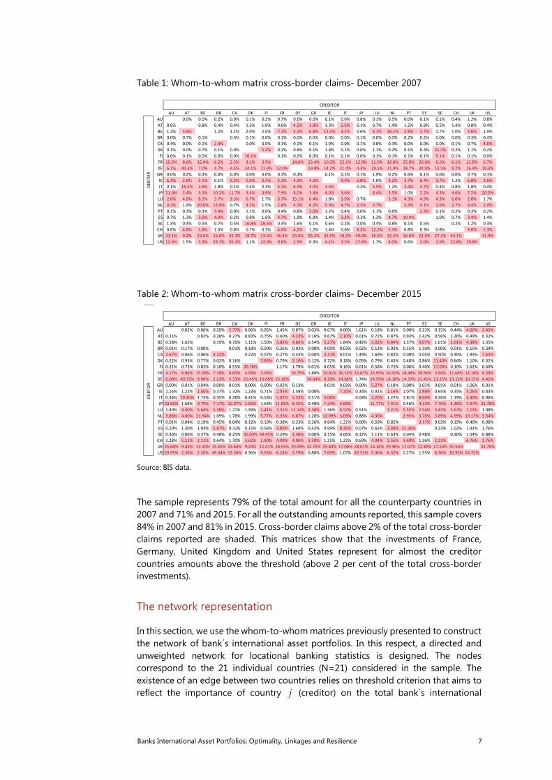
The whom-to-whom matrices permit tracing the debtor/creditor relationships between countries, i.e. they can be used to show asset balance sheet positions cross-classified by debtor country and creditor country. Based on the bilateral BIS statistical information on LBS/R, these matrices were constructed for the selected sample in December 2007 and 2015 (Tables 1 and 2).


Table 1: Whom-to-whom matrix cross-border claims- December 2007

Table 2: Whom-to-whom matrix cross-border claims- December 2015

Source: BIS data.

The sample represents 79% of the total amount for all the counterparty countries in 2007 and 71% and 2015. For all the outstanding amounts reported, this sample covers 84% in 2007 and 81% in 2015. Cross-border claims above 2% of the total cross-border claims reported are shaded. This matrices show that the investments of France, Germany, United Kingdom and United States represent for almost the creditor countries amounts above the threshold (above 2 per cent of the total cross-border investments).

The network representation

In this section, we use the whom-to-whom matrices previously presented to construct the network of bank´s international asset portfolios. In this respect, a directed and unweighted network for locational banking statistics is designed. The nodes correspond to the 21 individual countries (N=21) considered in the sample. The existence of an edge between two countries relies on threshold criterion that aims to reflect the importance of country j (creditor) on the total bank´s international

AU AT BE BR CA DK FI FR DE GR IE IT JP LU NL PT ES SE CH UK USAU 0.0% 0.0% 0.2% 0.9% 0.1% 0.2% 0.7% 0.6% 0.0% 0.1% 0.0% 0.8% 0.1% 0.5% 0.0% 0.1% 0.1% 0.4% 1.2% 0.8%AT 0.6% 0.8% 0.4% 0.4% 1.3% 1.0% 0.6% 4.5% 3.8% 1.3% 2.6% 0.1% 0.7% 1.4% 1.2% 0.8% 0.5% 1.4% 0.8% 0.4%BE 1.2% 4.6% 1.2% 1.1% 2.0% 2.0% 7.1% 4.2% 6.8% 12.5% 3.5% 0.6% 4.1% 16.1% 4.8% 3.7% 1.7% 1.0% 4.6% 1.9%BR 0.0% 0.7% 0.1% 0.3% 0.1% 0.0% 0.1% 0.0% 0.0% 0.0% 0.0% 0.1% 0.0% 0.0% 0.2% 0.2% 0.0% 0.0% 0.3% 0.4%CA 0.4% 0.0% 0.1% 2.4% 0.0% 0.0% 0.1% 0.1% 0.1% 1.9% 0.0% 0.1% 0.0% 0.3% 0.0% 0.0% 0.0% 0.1% 0.7% 4.6%DK 0.1% 0.0% 0.7% 0.1% 0.0% 5.2% 0.2% 0.8% 0.1% 1.4% 0.1% 0.0% 1.1% 0.2% 0.1% 0.3% 21.3% 0.2% 1.1% 0.2%FI 0.0% 0.1% 0.0% 0.0% 0.0% 10.1% 0.1% 0.2% 0.0% 0.1% 0.1% 0.0% 0.1% 0.1% 0.1% 0.1% 9.1% 0.1% 0.1% 0.0%

FR 10.2% 8.6% 15.4% 6.2% 2.5% 3.1% 3.9% 14.6% 15.4% 10.2% 22.1% 12.8% 11.0% 10.8% 22.0% 20.6% 6.5% 6.1% 12.8% 6.7%DE 6.1% 40.3% 7.0% 4.7% 4.5% 24.1% 11.9% 12.0% 19.8% 14.2% 21.4% 4.3% 29.5% 11.8% 18.7% 24.9% 13.5% 8.2% 16.9% 10.3%GR 0.0% 0.2% 0.3% 0.0% 0.0% 0.0% 0.0% 0.3% 0.3% 0.1% 0.1% 0.1% 1.9% 0.2% 0.6% 0.1% 0.0% 0.0% 0.7% 0.1%IE 6.3% 2.8% 2.1% 0.1% 5.2% 5.0% 2.5% 2.2% 4.3% 4.2% 9.9% 2.8% 1.0% 3.2% 3.7% 6.4% 3.7% 1.2% 6.8% 3.6%IT 0.1% 16.5% 2.6% 1.8% 0.1% 0.4% 0.3% 4.1% 6.3% 3.0% 3.3% 0.2% 5.5% 1.2% 2.4% 3.7% 0.4% 0.8% 1.8% 0.4%JP 21.0% 2.4% 5.5% 10.2% 11.7% 3.4% 3.9% 7.9% 8.0% 3.4% 4.0% 3.6% 8.4% 3.5% 1.0% 2.2% 4.3% 4.6% 7.2% 20.0%

LU 2.6% 4.6% 8.2% 3.7% 3.5% 6.7% 1.7% 6.7% 15.1% 6.4% 1.8% 5.9% 0.7% 3.1% 4.3% 4.9% 4.3% 6.0% 2.0% 1.7%NL 3.3% 1.9% 20.6% 12.9% 0.7% 3.3% 1.5% 2.6% 4.3% 6.2% 5.0% 4.7% 2.3% 3.7% 3.3% 4.1% 2.6% 2.7% 9.4% 2.9%PT 0.1% 0.3% 0.3% 3.4% 0.0% 1.1% 0.0% 0.4% 0.8% 2.0% 1.2% 0.4% 0.0% 1.1% 0.6% 2.3% 0.1% 0.2% 0.3% 0.2%ES 0.7% 1.3% 3.0% 4.9% 0.2% 0.8% 1.6% 4.7% 1.9% 0.9% 1.4% 3.2% 0.3% 1.3% 4.7% 19.4% 1.0% 0.7% 3.4% 1.4%SE 1.3% 0.4% 0.5% 0.7% 0.5% 16.8% 28.3% 0.4% 1.6% 0.1% 0.6% 0.2% 0.0% 0.4% 0.8% 0.1% 0.5% 0.2% 1.2% 0.3%

CH 0.6% 4.8% 5.8% 1.3% 0.8% 0.7% 0.3% 4.0% 4.2% 1.2% 1.4% 0.6% 8.3% 12.2% 5.3% 0.8% 0.3% 0.8% 9.0% 2.3%UK 33.1% 9.2% 23.6% 16.6% 32.3% 19.7% 13.6% 36.4% 25.6% 26.2% 35.5% 18.2% 49.0% 16.5% 32.2% 16.6% 22.6% 27.2% 43.1% 41.9%US 12.3% 1.5% 3.3% 29.1% 35.2% 1.1% 22.0% 9.6% 2.5% 0.3% 4.1% 3.3% 17.4% 1.7% 4.0% 0.6% 2.0% 2.9% 22.8% 19.8%

CREDITOR

DEBT

OR

AU AT BE BR CA DK FI FR DE GR IE IT JP LU NL PT ES SE CH UK USAU 0.02% 0.06% 0.29% 2.77% 0.06% 0.05% 1.45% 0.87% 0.03% 0.67% 0.00% 1.61% 0.18% 0.81% 0.00% 0.23% 0.15% 0.44% 4.66% 2.45%AT 0.21% 0.82% 0.26% 0.27% 0.83% 0.75% 0.60% 4.33% 0.16% 0.67% 2.10% 0.01% 0.72% 0.87% 0.93% 1.42% 0.56% 1.26% 0.49% 0.32%BE 0.58% 1.65% 0.19% 0.76% 1.11% 1.50% 3.83% 4.86% 0.54% 5.27% 1.84% 0.42% 3.02% 9.84% 1.37% 3.07% 1.01% 2.01% 4.38% 1.35%BR 0.01% 0.17% 0.00% 0.01% 0.18% 0.00% 0.26% 0.03% 0.00% 0.00% 0.03% 0.02% 0.13% 0.03% 0.15% 1.50% 0.00% 0.01% 0.15% 0.39%CA 2.67% 0.06% 0.06% 3.32% 0.22% 0.07% 0.27% 0.43% 0.00% 2.31% 0.01% 1.49% 1.69% 0.83% 0.00% 0.05% 0.50% 0.30% 1.93% 7.65%DK 0.22% 0.95% 0.77% 0.02% 0.16% 7.80% 0.79% 2.10% 0.12% 0.72% 0.18% 0.05% 0.79% 0.45% 0.40% 0.86% 21.40% 0.64% 1.10% 0.32%FI 0.21% 0.72% 0.82% 0.10% 0.55% 30.78% 1.17% 1.79% 0.01% 0.05% 0.16% 0.01% 0.58% 0.72% 0.06% 0.40% 17.03% 0.10% 1.62% 0.60%

FR 4.17% 6.86% 25.58% 7.10% 4.00% 4.93% 3.05% 10.75% 1.88% 13.61% 30.12% 15.87% 15.99% 10.32% 18.44% 29.66% 3.94% 11.64% 12.18% 6.28%DE 6.08% 40.72% 9.96% 2.23% 5.33% 10.45% 10.68% 15.18% 54.64% 8.28% 14.86% 1.74% 24.59% 18.18% 14.37% 21.41% 13.25% 13.12% 10.15% 4.42%GR 0.00% 0.01% 0.04% 0.00% 0.01% 0.00% 0.00% 0.02% 0.13% 0.01% 0.03% 0.00% 5.27% 0.18% 0.00% 0.02% 0.01% 0.01% 1.06% 0.01%IE 1.16% 1.22% 2.50% 0.37% 1.32% 1.23% 0.71% 2.05% 1.58% 0.08% 7.20% 0.34% 0.91% 2.16% 1.07% 2.88% 0.65% 0.35% 3.26% 0.83%IT 0.34% 19.45% 1.73% 0.35% 0.28% 0.41% 0.53% 5.02% 5.33% 0.51% 3.06% 0.04% 3.26% 1.22% 1.81% 8.60% 0.26% 1.19% 3.40% 0.96%JP 30.60% 1.68% 9.79% 7.17% 10.07% 2.90% 1.64% 11.89% 8.35% 0.48% 7.34% 4.88% 11.77% 7.41% 0.46% 4.23% 7.70% 4.28% 7.97% 31.78%

LU 1.40% 3.40% 5.64% 5.38% 1.21% 1.39% 2.41% 7.31% 11.14% 2.38% 1.36% 6.52% 0.51% 3.21% 5.55% 2.54% 3.47% 5.67% 2.13% 1.08%NL 3.88% 4.80% 21.94% 1.69% 1.78% 1.99% 5.77% 6.35% 6.87% 1.20% 12.09% 3.09% 0.88% 4.30% 2.95% 3.78% 3.69% 4.99% 10.17% 3.34%PT 0.01% 0.04% 0.19% 0.45% 0.04% 0.12% 0.19% 0.38% 0.33% 0.36% 0.84% 1.21% 0.00% 0.59% 0.82% 3.17% 0.02% 0.19% 0.40% 0.08%ES 0.20% 1.30% 1.93% 5.87% 0.31% 0.15% 0.56% 3.89% 1.69% 0.42% 0.99% 8.36% 0.07% 0.65% 3.48% 31.35% 0.23% 1.02% 1.93% 1.76%SE 0.36% 0.06% 0.37% 0.48% 0.25% 30.03% 39.45% 0.29% 2.48% 0.06% 0.15% 0.06% 0.12% 1.11% 0.63% 0.04% 0.48% 0.30% 1.54% 0.88%

CH 1.28% 5.11% 2.11% 0.64% 1.70% 3.62% 2.90% 4.09% 4.06% 3.50% 1.25% 1.22% 0.69% 4.94% 2.56% 3.69% 1.36% 2.21% 6.76% 2.76%UK 25.68% 9.43% 13.50% 15.05% 15.64% 9.24% 12.41% 28.93% 29.09% 32.75% 33.64% 17.06% 28.61% 14.16% 29.96% 17.07% 12.80% 17.54% 35.56% 32.76%US 20.95% 2.36% 2.20% 49.04% 53.56% 0.36% 9.53% 6.24% 3.79% 0.88% 7.69% 1.07% 47.53% 5.36% 6.32% 0.27% 1.55% 6.36% 16.92% 24.72%

CREDITOR

DEBT

OR


portfolio assets ( )IAP of country i (debtor). The threshold is set at 2 per cent of total bank´s international asset portfolios. Hence, the edge is directed from a country i to a country j , if country i bank´s international asset portfolio in country j is larger than the threshold. More formally:

𝑎𝑎𝚤𝚤,𝚥𝚥��⃗ = �1, 𝑖𝑖𝑖𝑖 𝐼𝐼𝐼𝐼𝐼𝐼𝑖𝑖;𝑗𝑗𝐼𝐼𝐼𝐼𝐼𝐼𝑗𝑗

> 0.02𝑖𝑖𝑓𝑓𝑓𝑓 𝑒𝑒𝑎𝑎𝑒𝑒ℎ 𝑒𝑒𝑓𝑓𝑐𝑐𝑐𝑐𝑐𝑐𝑓𝑓𝑐𝑐 𝑖𝑖 ≠ 𝑗𝑗, 𝑗𝑗 = 1,2, … 21

0, 𝑓𝑓𝑐𝑐ℎ𝑒𝑒𝑓𝑓𝑒𝑒𝑖𝑖𝑒𝑒𝑒𝑒

where 𝐼𝐼 = �𝑎𝑎𝑖𝑖,𝑗𝑗� is the 𝑁𝑁𝑁𝑁𝑁𝑁 connectivity or adjacency matrix.

The choice of this threshold ensures that the resulting network easy to interpret and visualise, while capturing the relevant interrelations between nodes.

The analysis in this paper disregards the strength of the edges identified using the binary information contained in the data (unweighted network). Since the network is directed, every node has two different degrees: indegree and outdegree. The indegree is the number of incoming edges, whereas the outdegree is the number of outgoing edges.

Formally, the number of indegrees is given by:

∑=

=N

rji

ins ad

1

And the number of outdegrees is given by:

∑=

=N

rij

outs ad

1

Figure 1 shows the network representations for bank´s international asset portfolio for two distinct periods: December 2007 (before the financial crises) and March 2016 (the most recent available period).

As previously mentioned, the network is directed and the arrows represent the edges, pointing towards countries which threshold is above 2% of the total banks asset holdings.


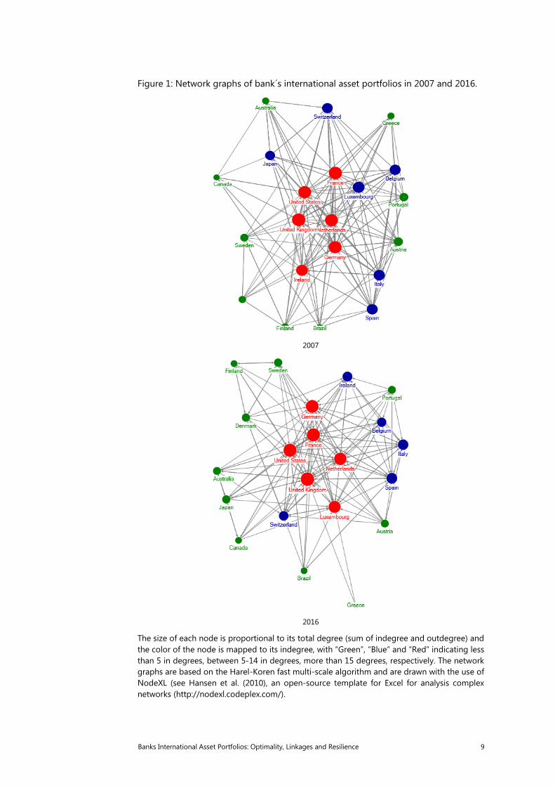
Figure 1: Network graphs of bank´s international asset portfolios in 2007 and 2016.

2007

2016

The size of each node is proportional to its total degree (sum of indegree and outdegree) and the color of the node is mapped to its indegree, with “Green”, “Blue” and “Red” indicating less than 5 in degrees, between 5-14 in degrees, more than 15 degrees, respectively. The network graphs are based on the Harel-Koren fast multi-scale algorithm and are drawn with the use of NodeXL (see Hansen et al. (2010), an open-source template for Excel for analysis complex networks (http://nodexl.codeplex.com/).


Each country is represented by a circle (node) with arrows (edges) directed from the investor (debtor) to the counterparty country (creditor - who holds the bank´s international assets). In this setup, a force directed layout algorithm is typically used to determine the location of the nodes in the network visualisation. All network graphs in this article are based on the Harel-Koren fast muti-scale alogorithm (Haren and Koren 2002) and are drawn with the use of NodeXL (Hansen et al. 2010). The colour of each node is mapped to its indegree, with “Green”, “Blue” and “Red” indicating less than 5 in degrees, between 5-14 in degrees, more than 15 degrees, respectively.

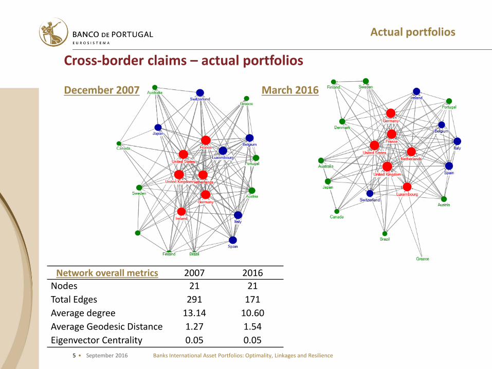
Larger countries tend to have bigger nodes and to locate in the center of the network, because they hold an important amount of the bank´s international asset portfolios. Smaller economies tend to locate in the outer layers of the network. Usually its banks invest their international assets abroad and the other countries do not invest there. Given the construction of the network, it is natural that the large are at the centre but there are other things. Ireland is in this group, there are some interesting linkages between the countries outside this core group.

Between 2007 and 2016 there are some changes in the number of edges and in the position of nodes in the network. In 2007, there are six core countries (with more than 15 indegrees) – UK, USA, DE, FR, IE and NL. In 2016, there are five core countries - UK, USA, NL, FR and LU. (DE and IE are not core countries in the first quarter of 2016 but LU). Austria increased the number of indegrees in 2016.

Metrics

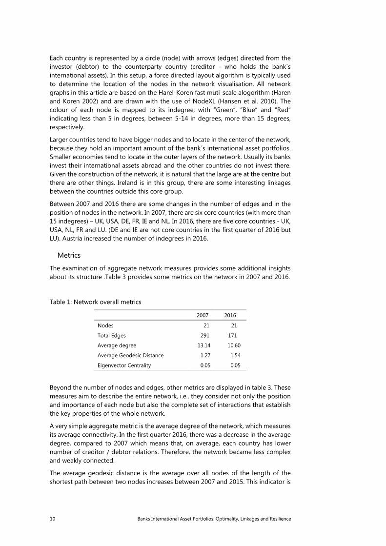
The examination of aggregate network measures provides some additional insights about its structure .Table 3 provides some metrics on the network in 2007 and 2016.

Table 1: Network overall metrics

2007 2016

Nodes 21 21

Total Edges 291 171

Average degree 13.14 10.60

Average Geodesic Distance 1.27 1.54

Eigenvector Centrality 0.05 0.05

Beyond the number of nodes and edges, other metrics are displayed in table 3. These measures aim to describe the entire network, i.e., they consider not only the position and importance of each node but also the complete set of interactions that establish the key properties of the whole network.

A very simple aggregate metric is the average degree of the network, which measures its average connectivity. In the first quarter 2016, there was a decrease in the average degree, compared to 2007 which means that, on average, each country has lower number of creditor / debtor relations. Therefore, the network became less complex and weakly connected.

The average geodesic distance is the average over all nodes of the length of the shortest path between two nodes increases between 2007 and 2015. This indicator is


lower in 2015 when compared to 2007 meaning that in 2015, these 21 economies are less integrated.

The eigenvector centrality is an aggregate metric that characterises how a network is centred around one or a few important nodes by examining the differences in centrality between the most central node in a network and all others. This measure ranges between and allows us to take basic inferences regarding the resilience of the network to shocks.

Optimal cross-border portfolios

In this section we perform a stylized exercise aiming at the identification of what would be the banks’ optimal cross-border portfolios. This is a conceptual exercise because the decision of banks relatively to where assets should be placed depends on more parameters than past observed volatility and return. For example geographical proximity, historical and political linkages certainly play a role. In addition, the exercise does not consider the possibility of short portfolios, i.e., banks’ having liabilities versus other locations, or holding assets in the domestic banking system. These options are to be tried in a future version of the paper.

In order to compute the optimal cross-border portfolio we apply the standard theory that assesses the return and risk components of banks’ portfolio choices.

The portfolio risk comes from the covariances of its different assets, while the marginal contribution to return variance is measured by the covariance between the asset’s and portfolio’s return rather than by the variance of the asset itself.

On the basis of this model, banks located in each country will decide in which countries to invest their assets in order to maximise asset returns. However, in their decision risk component is integrated to avoid excessive exposure to external market risk.

In order to determine the optimal portfolio, it is assumed that asset returns follow three main indicators equally weighted: i) the change rate of the individual stock market country indexes for all the countries in the sample; ii) exchange rate change; iii) change rate of dividend yiels (10 years). These data was obtained on a daily basis between 1st January 2001 and 25 February 2016 but it was considered that banks take portfolio investment decisions with information regarding the latest 1.5 years.

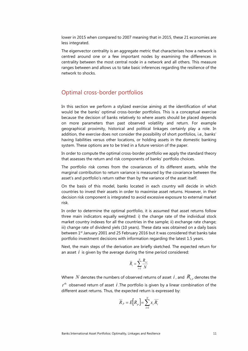
Next, the main steps of the derivation are briefly sketched. The expected return for an asset i is given by the average during the time period considered:

∑=

=N

t

tii N

RR

1

,

Where N denotes the numbers of observed returns of asset i , and tiR , denotes the tht observed return of asset i .The portfolio is given by a linear combination of the

different asset returns. Thus, the expected return is expressed by:

[ ] ∑=

==N

iiipp RxRER

1


where N

xi1

= denotes the proportion of asset i held in the portfolio. It is assumed

that there is no short selling, i.e., capital can only be obtained with recourse of own savings, Nixi ,...2,1,0 => . In addition, total asset´s proportion has to be equal to

the total capital available: ∑=

=N

iix

11 .

The risk of each asset i is defined by its dispersion - the standard deviation:

( )( )∑

= −−

=N

t

itii N

RR

1

2,

1σ

And the correspondent portfolio is given by:

( )∑ ∑∑= =

≠=

+=N

j

N

j

N

jkk

kjkjjjp xxx1 1 1

,22 σσσ

Where kj ,σ denotes the covariance between asset j and k :

( ) ( )( )( )∑

= −

−−==

N

t

ktkjtjkjkj N

RRRRRR

1

,,, 1

,covσ

Moreover, ρ is the correlation coefficient between assets A and B which is always between -1 and 1 and is expressed as follows:

( )BA

BA RRσσ

ρ ,cov=

The optimal diversification model finds the composition of all the portfolios that correspond to the efficiency criterion defined for a given set of assets, and construct the corresponding efficient frontier. It minimizes the risk for a given return or maximizes the return for a given risk, which can be written as follows:

{ }

[ ]

∑=

=

=N

ii

p

pp

x

EREtos

Min

1

2

1

..

σ

The constant correlation model is applied to calculate the optimal portfolios. This method is based on an optimal ranking of the assets, established over the simplified correlation representation model. To determine the optimal portfolio, the Sharp ratio is calculated for all the available assets:


[ ]i

fi RRESR

σ−

=

Where [ ]iRE denotes the expected return on asset i ; fR denotes the risk-free rate;

and iσ denotes the standard deviation of the return of asset i .

The results are classified from the highest value (more desirable) to the lowest value (less desirable) to hold in the portfolio. A threshold is determined to decide which assets will be part of the optimal portfolio (those above the threshold) assets below the threshold will be excluded. The cut-off point *C is computed as follows:

∑=

−

+−=

i

j j

fj RRi

C1

*

1 σρρρ

Where jR denotes the expected return on security j , jσ denotes the standard

deviation of the return of asset j , and ρ denotes the constant correlation coefficient:

( )2

1

1 1,

−=

∑∑=

≠=

NN

N

i

N

ijj

jiρ

ρ

Where ji,ρ denotes the correlation between assets i and j ; and N denotes the

number of assets in the portfolio. N was used earlier for the number of returns observed for each asset.

The weight of each asset is expressed as:

∑=

= N

ii

ii

Z

Zx

1

where ( )

( )

−

−

−= *

11 C

RRZ

i

fi

ii σρσ

We show the results using the network representation that emerge from the optimal portfolios before and after the crisis. The first period before the crises is considered between January 2006 and June 2007. The period after the crises corresponds to June 2012 and November 2013.

The comparison of the optimal portfolios with those that actually existed must be cautious because other aspects determine bank’s international decisions. For example, the deviations between the actual and the benchmark portfolios may be attributable to factors that affect the risk and returns from cross-border asset holdings as Regulations, institutions and information costs that produce frictions as in Buch et al. (2010). Another caveat relatively to the concept of a global optimal


portfolio allocation should be mentioned. The optimal portfolio is based on a partial equilibrium approach because it assumes that decisions of reallocation towards some country can always be implemented. However, even if it is optimal to reallocate towards some country, the supply of assets available may be limited, especially if the destination country is small and most source countries are reallocating in the same way. Therefore, the excess demand for the assets increases their price and reduces the implicit rate of return, leading to a new optimal portfolio.

Nevertheless, some insights emerge from the exercise performed. In order to highlight these differences we make use of the network presented in section three – Mapping the network of cross-border portfolios to map the linkages that would arise from banks’ international optimal asset portfolios (Figure 2).


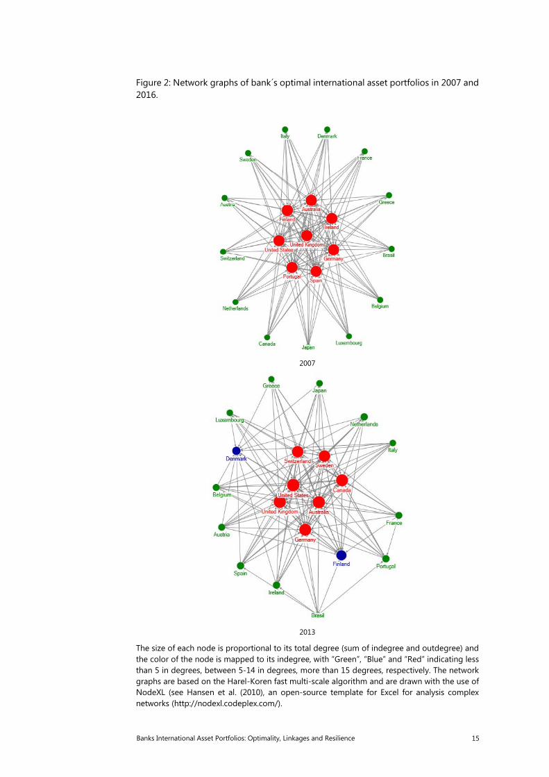
Figure 2: Network graphs of bank´s optimal international asset portfolios in 2007 and 2016.

2007

2013

The size of each node is proportional to its total degree (sum of indegree and outdegree) and the color of the node is mapped to its indegree, with “Green”, “Blue” and “Red” indicating less than 5 in degrees, between 5-14 in degrees, more than 15 degrees, respectively. The network graphs are based on the Harel-Koren fast multi-scale algorithm and are drawn with the use of NodeXL (see Hansen et al. (2010), an open-source template for Excel for analysis complex networks (http://nodexl.codeplex.com/).

http://nodexl.codeplex.com/


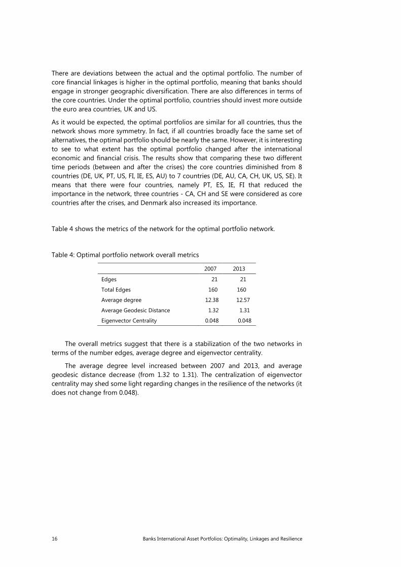
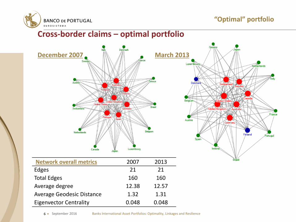
There are deviations between the actual and the optimal portfolio. The number of core financial linkages is higher in the optimal portfolio, meaning that banks should engage in stronger geographic diversification. There are also differences in terms of the core countries. Under the optimal portfolio, countries should invest more outside the euro area countries, UK and US.

As it would be expected, the optimal portfolios are similar for all countries, thus the network shows more symmetry. In fact, if all countries broadly face the same set of alternatives, the optimal portfolio should be nearly the same. However, it is interesting to see to what extent has the optimal portfolio changed after the international economic and financial crisis. The results show that comparing these two different time periods (between and after the crises) the core countries diminished from 8 countries (DE, UK, PT, US, FI, IE, ES, AU) to 7 countries (DE, AU, CA, CH, UK, US, SE). It means that there were four countries, namely PT, ES, IE, FI that reduced the importance in the network, three countries - CA, CH and SE were considered as core countries after the crises, and Denmark also increased its importance.

Table 4 shows the metrics of the network for the optimal portfolio network.

Table 4: Optimal portfolio network overall metrics

2007 2013

Edges 21 21

Total Edges 160 160




The overall metrics suggest that there is a stabilization of the two networks in terms of the number edges, average degree and eigenvector centrality.

The average degree level increased between 2007 and 2013, and average geodesic distance decrease (from 1.32 to 1.31). The centralization of eigenvector centrality may shed some light regarding changes in the resilience of the networks (it does not change from 0.048).


Final remarks

Although financial markets became more integrated over the years, after the economic and financial crises there was some reduction of the cross-border assets and questions relating to the reshaping international banks portfolios of and its resilience to shocks emerged in the policy-debate.

The whom-to-whom portfolio matrices provide basic information regarding the identification of the main linkages. In this context, network theory offers convenient visualization tools that provide interesting insights in terms of the cross-border banks’ portfolio. In addition, it is interesting to assess how large are deviations between actual portfolios and those that would result from the optimal portfolio theory.

The paper concludes that with the financial crises the international linkages between countries changed and the number of core countries diminished. Some countries moved their position in the network. In particular, vulnerable economies deviated from the centre after the financial crisis.

When comparing to the optimal portfolio it deviates significantly from the actual one (before and after the crisis) more diversification needed. More countries appear in the centre. The network that corresponds to the optimal portfolio has also changed with the crisis. In 2013, the core countries changed – Portugal, Spain and Ireland deviated from the centre while new countries – Canada, Sweden and Switzerland became the core countries.

The analysis performed in this paper is admittedly very preliminary and important caveats limit the interpretation of results. However, the utilization of network methods in connection with the concept of an optimal global portfolio seems to be a promising avenue for further research.

References

Amador, J. and Cabral, S. (2015): “Networks of value added trade”. Banco de Portugal, Working Paper 16.

Bank for International Settlements (2013): “Guidelines for reporting the BIS international banking statistics”

Bremus, F., Fratzscher, M. (2015): “Drivers of structural change in cross-border banking since the global financial crisis”. Journal of International Monetary and Finance 52: 32-59.

Buch, C. M., J.C. Driscoll, and C. Ostergaard (2010): “Cross-border diversification in bank asset portfolios”. International Finance 13(1): 79–108.

Committee on International Economic Policy and Reform (2012): “Banks and Cross-Border Capital Flows: Policy Challenges and Regulatory Responses”. Rethinking central banking, Brookings Institution, September.

Hills, B. and Hoggarth, G. (2013): “Cross-border bank credit and global financial stability”, Quarterly Bulletin 2013 Q2 Bank of England.

http://onlinelibrary.wiley.com/doi/10.1111/j.1468-2362.2010.01253.x/full

http://onlinelibrary.wiley.com/doi/10.1111/j.1468-2362.2010.01253.x/full


Hoggarth, G, Mahadeva, L and Martin, J (2010): “Understanding international bank capital flows during the recent financial crisis”, Bank of England Financial Stability Paper No. 8.

Joseph, A., Joseph, S. and Chen, G. (2014): “Cross-border Portfolio Investment Networks and Indicators for Financial Crises”, Scientific Reports vol. 4(3991).

Eighth IFC Conference on “Statistical implications of the new financial landscape”

Basel, 8–9 September 2016

Banks international asset portfolios: optimality, linkages and resilience1 João Amador and João Falcão Silva,

Bank of Portugal

1 This presentation was prepared for the meeting. The views expressed are those of the authors and do not necessarily reflect the views of the BIS, the IFC or the central banks and other institutions represented at the meeting.

Meeting 2016 IFC Conference

João Amador & João Falcão Silva• Research Department and Statistics DepartmentSeptember 2016

Banks International Asset Portfolios: Optimality, Linkages and Resilience

2 •

Introduction

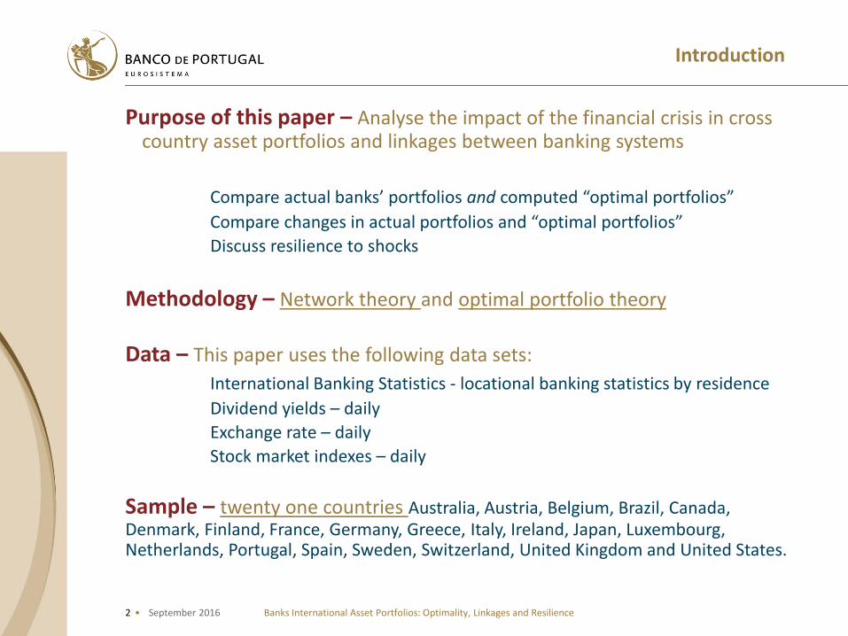
Purpose of this paper – Analyse the impact of the financial crisis in cross country asset portfolios and linkages between banking systems

Compare actual banks’ portfolios and computed “optimal portfolios”

Compare changes in actual portfolios and “optimal portfolios”

Discuss resilience to shocks

Methodology – Network theory and optimal portfolio theory

Data – This paper uses the following data sets:

International Banking Statistics - locational banking statistics by residence

Dividend yields – daily

Exchange rate – daily

Stock market indexes – daily

Sample – twenty one countries Australia, Austria, Belgium, Brazil, Canada, Denmark, Finland, France, Germany, Greece, Italy, Ireland, Japan, Luxembourg, Netherlands, Portugal, Spain, Sweden, Switzerland, United Kingdom and United States.

Banks International Asset Portfolios: Optimality, Linkages and ResilienceSeptember 2016

3 •

Data

Locational Banking Statistics analysis

International banking activity - Cross-border claims outstanding amount - 883 billion of USD (1978) 26536 billions of USD (2015)

Financial and economic crisis period - annual change rate -6.9% in 2008 (United Kingdom, Portugal, Italy, Ireland, Greece and Spain, USA and Switzerland)


4 •

Network of bank international asset portfolios

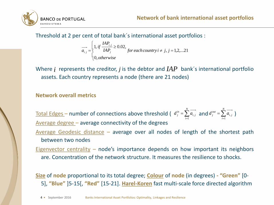
Threshold at 2 per cent of total bank´s international asset portfolios :

Where represents the creditor, is the debtor and bank´s international portfolio

assets. Each country represents a node (there are 21 nodes)

Network overall metrics

Total Edges – number of connections above threshold ( and )

Average degree – average connectivity of the degrees

Average Geodesic distance – average over all nodes of length of the shortest path

between two nodes

Eigenvector centrality – node’s importance depends on how important its neighbors

are. Concentration of the network structure. It measures the resilience to shocks.

Size of node proportional to its total degree; Colour of node (in degrees) - “Green” [0-

5], “Blue” ]5-15[, “Red” [15-21]. Harel-Koren fast multi-scale force directed algorithm


21,...2,1,

,0

,02.0,1,

.

jjicountryeachfor

otherwise

IAP

IAPif

a j

ji

ji

i j IAP

N

i

ji

in

j ad1

,

N

i

ji

out

j ad1

,

5 •

Actual portfolios

Cross-border claims – actual portfolios

December 2007 March 2016


Network overall metrics 2007 2016

Nodes 21 21

Total Edges 291 171




6 •

“Optimal” portfolio

Cross-border claims – optimal portfolio

December 2007 March 2013


Network overall metrics 2007 2013

Edges 21 21

Total Edges 160 160




7 •

Main conclusions

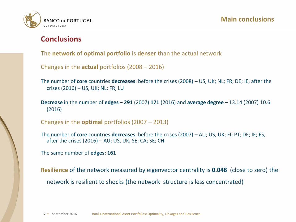
Conclusions

The network of optimal portfolio is denser than the actual network

Changes in the actual portfolios (2008 – 2016)

The number of core countries decreases: before the crises (2008) – US, UK; NL; FR; DE; IE, after the crises (2016) – US, UK; NL; FR; LU

Decrease in the number of edges – 291 (2007) 171 (2016) and average degree – 13.14 (2007) 10.6 (2016)

Changes in the optimal portfolios (2007 – 2013)

The number of core countries decreases: before the crises (2007) – AU; US, UK; FI; PT; DE; IE; ES,after the crises (2016) – AU; US, UK; SE; CA; SE; CH

The same number of edges: 161

Resilience of the network measured by eigenvector centrality is 0.048 (close to zero) the

network is resilient to shocks (the network structure is less concentrated)


8 •

Thank you for your attention!

Questions?

João Falcão [email protected]

mailto:[email protected]

Documents

Banks international asset portfolios: optimality, linkages ... · Banks international asset portfolios: optimality, ... 4 Banks International Asset Portfolios: Optimality, Linkages