Creating Composite Measures - John Jay College of …jjcweb.jjay.cuny.edu/...creating_composite_measures-compute-if.pdfLECTURE CRJ 716: Chapter 6 – Creating Composite Measures Chapter

LECTURE

CRJ 716: Chapter 6 – Creating Composite Measures

Chapter 6: Creating Composite Measures Prof. Kaci Page 1 of 18

Creating Composite Measures

Lecture 6: Computing Variables

CRJ 716 – Using Computers in Social Research

Prof. Agron Kaci John Jay College

LECTURE



Abstract Sometimes, in the criminal justice research, we will need to analyze a single concept not only from one indicator, but from multiple indicators' point of view. Occasionally, analyzing just one variable at a time

will not yield the desirable and complete result. Therefore, we will need to measure a few pieces of

information together. One classical example is measuring up what’s called the ―crime index‖, which is made up of seven crime categories: murder and nonnegligent manslaughter, forcible rape, robbery,

aggravated assault, burglary, larceny and theft, and motor-vehicle theft. Each of these crimes may have a separate variable in a data set and in order to measure them, we may need to sum all of them up and

create a new variable, ―crime index‖. This lecture will cover creating composite measures of different

variables of interest.

Creating Composite Measures Using COMPUTE

INTRODUCTION

We have observed in the 2004gss data set that there are seven variables regarding abortion (the original GSS file has more than 7 variables regarding abortion). The General Social Survey asks a question

regarding a woman’s right to obtain a legal abortion under various situations. The PreQuestion Text is: ―Please tell me whether or not you think it should be possible for a pregnant woman to obtain a legal abortion if:‖.

The literal questions make the variables listed below (circumstances are in parentheses):

ABANY (when woman wants abortion for any reason)

ABDEFECT (when there is strong chance of serious defect in the baby)

ABHLTH (woman's health seriously endangered)

ABNOMORE (woman wants no more children)

ABPOOR (woman is poor and can't afford more children)

ABRAPE (woman wants abortion when is pregnant as result of rape)

ABSINGLE (woman is not married).

Each variable has two valid answers: Yes coded as 1 and No coded as 2. The missing values are: 0-

NAP (Not APplicable), 8-DK (Don't Know), and 9-NA (No Answer).

We can run frequency reports on all seven individual variables regarding abortion and come up with

seven different tables, which would not make it fun at all to get a summarized analysis on them. What would make it fun, or at least easy? …Having only one frequency table for all seven variables!

Luckily for us, SPSS has a command, Compute, that allows us to sum all of these seven variables into

one. The way compute works is by adding the values (remember: values are codes/numbers and SPSS is thrilled to have to work with numbers) of different variables together.

Since all of the ―seven‖ have the same set of answers (1 for Yes and 2 for No), when we add them together we will get various values. Let’s say that a participant answered "Yes" to all seven questions. In

this case, the respondent’s sum (or new value) would be 7 (=7 Yes answers times 1, which is the code

for Yes). In case all answers would have been "No" the new value will equal 14 (=7*2). And of course there would be new values in between, all of these answering differently for each question. The missing

values would be transferred as ―missing‖ in the newly computed variable.

Let’s start with an idea: do you think that there would be more respondents who approve of a woman to

get a legal abortion for any of the circumstances? Let’s say that a value of 7 (when answered all questions positively – Yes) will be high approval and a value of 14 would be no approval at all. We’ll

remember this when we’ll have to label the new values.

LECTURE



COMPUTE PROCEDURE

To start the Compute command, follow the steps in the diagram below:

Figure 6- 1

SPSS will then, display the Compute Variable dialog box. There is no reason to hide now! The electronic calculator is not that frightening… we’ll deal with it shortly.

In the dialog box, the first step we’ll undertake will be to give a name to the new variable. Let’s call it

ABORTION. So, go ahead and type ―ABORTION‖ in the Target Variable field. Now, this new variable will be equal to the sum of the seven individual variables. So click to select variable ABANY in the list of

variables and then click the arrow to transfer this variable in the Numeric Expression field, to the right of the equal (=) sign. Then, click the plus (+) sign in the numeric calculator, or just press the ―+” key in

your keyboard. This denotes the start of the creation of our formula:

ABORTION= ABANY + ABDEFECT + ABHLTH + ABNOMORE + ABPOOR + ABRAPE + ABSINGLE

After entering the plus sign click on ABDEFECT in the list on the left and transfer it to the Numeric Expression field. Repeat the procedure until you’ve completed the formula depicted above and the screen looks like Figure 6.2 below.

Figure 6- 2

Click OK to finish the process. The new variable is created and will be found at the rightmost side in the

data table.

Transform Compute Variable

LECTURE



VARIABLE LABELS AND VALUE LABELS (ABORTION)

Double click the header of the ABORTION variable. This will take us to the Variable View and ready to change some or all of its properties. We will add a label for the variable — this would be the long name

of the variable – and value labels. Type in ―All Abortion variables summed up‖ as the Variable Label.

In the Values box click the little square button at the right side of the cell to go

to the Value properties area (see image at the right).

We said above that those who answered Yes to all abortion questions would receive a value of 7, therefore they would be the respondents who exhibited high

approval for a woman obtaining a legal abortion for any circumstance.

Thus, type in ―7‖ in the Value field of the Value Labels dialog box. Press Tab in your keyboard, or just click inside the field

next to Label, and type ―High Approval‖. Click Add to save this value label.

Go back to the Value field and type ―14‖. Consequently, type ―No Approval‖ in the Label field and click Add. 14 is the

new value that shows all those who answered No to all the

abortion questions, therefore yielding a value of 14 (7*2, where 2 is the code for the No answer).

We don’t need to create more value labels as all values between seven and fourteen represent different levels of

approvals; some approve more and some less. We are

interested in only those who approve all and those who approve none, meaning those who are pro and those who are against the right of a woman to obtain a

legal abortion.

FREQUENCY

Well, we didn’t just undertake a procedure like Compute, only to create a pretty new variable in the data set. We need to make use of it. What can we see and observe in this new variable that we couldn’t in all

abortion variables individually? The first step is to run a frequency test, to see the distribution of new groups that we created, especially those of high and no approval.

By now, the frequency procedure should be as easy as falling off a log. Wait, did someone say ―log‖ in a statistics course? OK, let’s just say that it should be as easy as pie…

Grab ABORTION variable and move it to the Variables box. Click OK and SPSS will produce the

frequency table as shown in the Table 6-1 below.

Analyze Descriptive Statistics Frequencies

Figure 6- 3

LECTURE



All Abortion Variables Summed Up

Frequency Percent Valid Percent

Cumulative Percent

Valid High Approval 137 11.4 43.4 43.4

8 16 1.3 5.1 48.4

9 20 1.7 6.3 54.7

10 21 1.8 6.6 61.4

11 50 4.2 15.8 77.2

12 21 1.8 6.6 83.9

13 23 1.9 7.3 91.1

No Approval 28 2.3 8.9 100.0

Total 316 26.3 100.0 Missing System 884 73.7 Total 1200 100.0

Table 6-1

We actually see that 137 respondent or 43.4% of those who gave a valid answer approve of a woman getting a legal abortion under any of the seven circumstances, while 28, or almost 9% do not approve

abortion at all. So, there is a small group of 9% of the population that do not support abortion at any cost. Can you come up with any ideas why? What can cause this attitude?

Why don’t you run a frequency table for ABANY (abortion if woman wants for any reason)? Check the

percentage of respondents who do not approve it and compare with those who belong to the ―No Approval‖ group in the table above.

COMPUTE RATIO (MAEDUC / PAEDUC)

As seen above, Compute is a powerful tool in SPSS. It doesn’t just add variable values. It can

multiply, divide, subtract, raise to a power, etc. Did someone say ―log‖ before? Yes, it can do that too!

Let’s try division… Because we are a curious breed, we will try to find out whose respondents’ parent has more education. The variables associated with these concepts are PAEDUC—father’s education—and

MAEDUC—mother’s education. The 2004gss.sav does not have these variables, since it's designed for use with SPSS Student edition, which limits the variable count to 50. So, for this example we will open

the 2008gss.sav file.

The idea here is to get the ratio of the mother’s education to the father’s education. To do this we need to divide variable MAEDUC by variable PAEDUC. So if we compute MAEDUC / PAEDUC we would get

a value that if it’s greater than one will mean that the mother’s education is greater than the father’s education and vice versa, if the father has more education, then the computed value will be smaller than

1. Of course, SPSS will calculate this ratio value for each respondent in the data set.

Before we start the Compute procedure we need to address a small issue. What if the father's education is zero? In that case the ratio value will be zero, since dividing by zero will always result in zero. Then, of

course a ratio value 0 will not give us the correct result. To overcome this problem we will change all values of the father’s education in the data set from 0 to 1. Dividing by 1 will give us the number of the

mother’s education. To change the value from 0 to 1, we would need to recall a useful procedure we learned in Chapter 5: Recode. We will recode PAEDUC into the same variable, only we will change

values that are entered as 0.

Recode

To conduct this procedure, follow the steps in the diagram below:

Transform Recode into Same Variables

LECTURE



Figure 6- 4

Don’t worry! We will not save the file in the end, so the change will not alter our data.

Transfer PAEDUC into the Numeric Variables box by double-clicking it or selecting and then clicking the

arrow.

Figure 6- 5

Click on the Old and New Values button. Replace 0 with 1 as depicted in the Figure 6-6 below. Click Add and then click Continue.

Figure 6- 6

Click OK in the Recode into Same Variables dialog box. The variable PAEDUC values 0 now have

changed to 1, meaning that those who reported that their father had 0 years of education are now

changed to 1 year of education. In reality, if you ran a frequency of PADUC, you would have found that there were 37 respondents, or 2.5%, who reported that their father had 0 years of school completed

(very brave indeed!) See table below:

LECTURE



Since we’ve now changed each 0 for PAEDUC into a 1, we are ready to create our ratio variable which

we will, incidentally of course, call RATIO.

To start the Compute command, follow the steps in the diagram below:

You may click the Reset button to empty out the field that’s occupied by the previous formula. Type

RATIO in the Target Variable field. The formula we talked of creating was MAEDUC/PAEDUC, so select

MAEDUC and transfer it into the Numeric Expression field. Press ―slash‖ key in your keyboard or just click ―/‖ in the numeric calculator, as depicted in the figure below. Now move PAEDUC after "/".

Figure 6- 7

SPSS will create the variable as soon as you click OK. Let's take a look at the data table in the Data Editor window in SPSS. If you are not there, go to the Data View window, by clicking on the tab located

in the lower-left corner of the window. Find the new variable, RATIO on the rightmost side of the table.

You may see missing values, denoted by periods (.). These are those cases where one or both variables are coded as missing.

Now, we may need to recode this new variable (RATIO), which incidentally is a ratio level variable, into another variable (RATIO1), where we would combine values into three distinct categories:

If RATIO < 1 Mother LESS education than Father (recode as 1)

If RATIO ≈ 1 Mother has same education as Father (recode as 2)

If RATIO > 1 Mother MORE education than Father (recode as 3)

So, new values of RATIO1 would be: 1=Mother less education, 2=Mother and Father same education,

and 3=Mother more education than father.

Transform Compute Variable

LECTURE



RECODE RATIO INTO RATIO1

To create this new variable RATIO1 we would use the familiar procedure Recode.

Find and transfer the variable RATIO in to the Numeric Variable box. Enter the new name RATIO1 in

the Name field. Type in a Label: ―RATIO Recoded‖. Click Old and New Values button to create new values for RATIO1.

Figure 6- 8

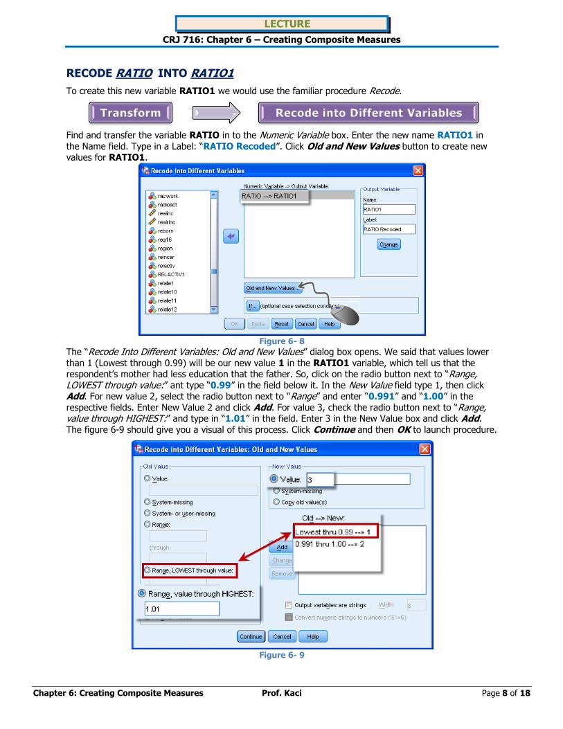
The ―Recode Into Different Variables: Old and New Values‖ dialog box opens. We said that values lower

than 1 (Lowest through 0.99) will be our new value 1 in the RATIO1 variable, which tell us that the respondent’s mother had less education that the father. So, click on the radio button next to ―Range, LOWEST through value:‖ ant type ―0.99‖ in the field below it. In the New Value field type 1, then click Add. For new value 2, select the radio button next to ―Range‖ and enter ―0.991‖ and ―1.00‖ in the

respective fields. Enter New Value 2 and click Add. For value 3, check the radio button next to ―Range, value through HIGHEST:‖ and type in ―1.01‖ in the field. Enter 3 in the New Value box and click Add.

The figure 6-9 should give you a visual of this process. Click Continue and then OK to launch procedure.

Figure 6- 9

Transform Recode into Different Variables

LECTURE



The next step would be to add labels to the new values we added, 1, 2, and 3.

VARIABLE LABELS AND VALUE LABELS (RATIO1)

In the Data editor window in SPSS, double click the header of the RATIO1 variable. This will take us to

the Variable View and ready to change some or all of its properties. We can add a label for the values. The Variable Label is already added.

In the Values box click the little square button at the right side of the cell to

go to the Value properties area (see image at the right).

Since we have only three categories that we designed beforehand, we

would need to label only values 1, 2, and 3, according to the list created above:

If RATIO < 1 Mother LESS education

than Father (recode as 1)

If RATIO ≈ 1 Mother has same

education as Father (recode as 2) If RATIO > 1 Mother MORE education

than Father (recode as 3)

Thus, type in ―1‖ in the Value field of the Value Labels dialog box. Press Tab in your keyboard, or

just click inside the field next to Label, and type ―Mother LESS Educ‖. Click Add to save this

value label.

Go back to the Value field and type ―2‖.

Consequently, type ―Same Education‖ in the Label field and click Add. Type ―3‖ in the Value

field and also enter ―Mother MORE Educ‖ in the

Label field and click Add, as shown in Figure 6-10 above. Click OK to create value labels.

One little stop here to remind you how to reduce the decimal points. If you’ve carefully observed, new

values are always created with two zeroes at the right of the decimal point. This is done by default in SPSS. If these decimals annoy you, you can remove them by clicking the lower arrow in the Decimals cell

in the Variable View window. See figure 6-11 for a visual.

Figure 6-11

FREQUENCY (RATIO1)

After we run the frequency procedure for the RATIO1 Recoded variable, SPSS Output provides us with a

frequency table, where three categories that we created are listed and their respective frequency occurrences, percents and valid percents.

Figure 6- 10

LECTURE



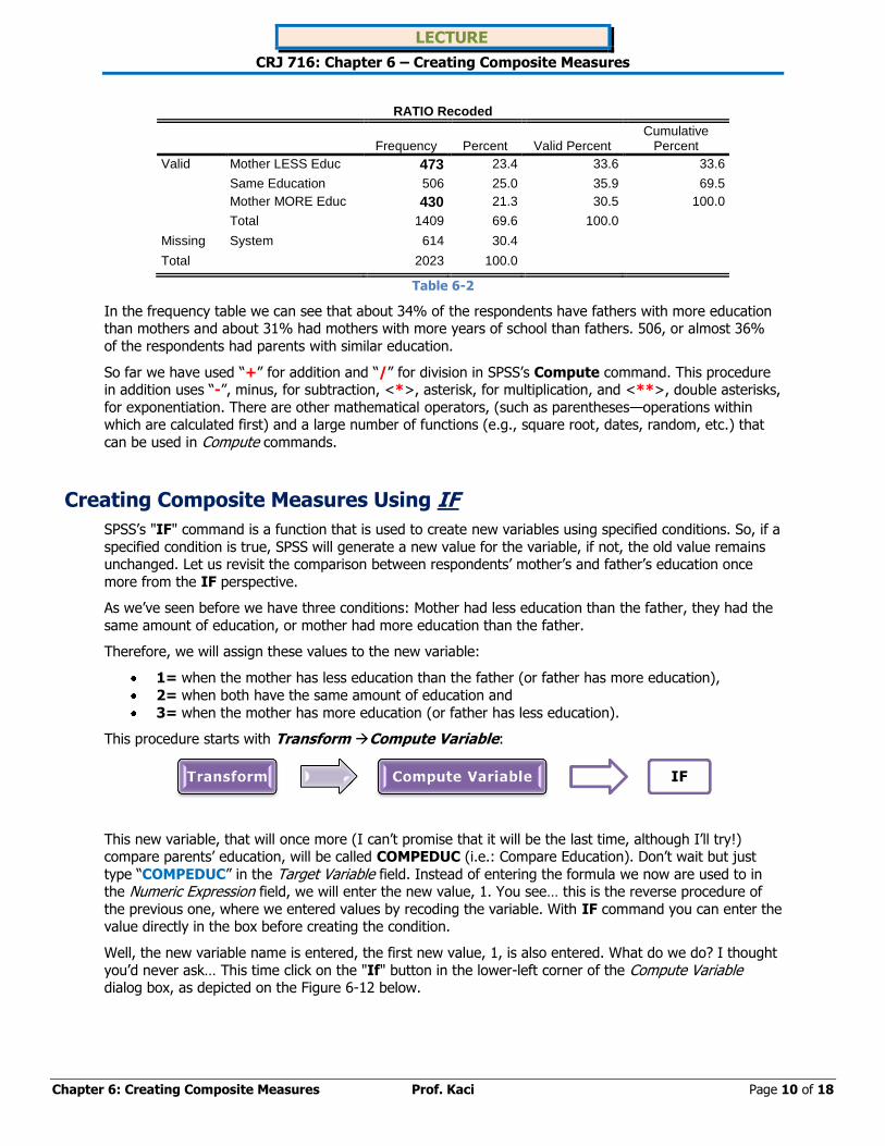
RATIO Recoded


Cumulative Percent

Valid Mother LESS Educ 473 23.4 33.6 33.6

Same Education 506 25.0 35.9 69.5

Mother MORE Educ 430 21.3 30.5 100.0


Table 6-2

In the frequency table we can see that about 34% of the respondents have fathers with more education than mothers and about 31% had mothers with more years of school than fathers. 506, or almost 36%

of the respondents had parents with similar education.

So far we have used ―+‖ for addition and ―/‖ for division in SPSS’s Compute command. This procedure in addition uses ―-‖, minus, for subtraction, <*>, asterisk, for multiplication, and <**>, double asterisks,

for exponentiation. There are other mathematical operators, (such as parentheses—operations within which are calculated first) and a large number of functions (e.g., square root, dates, random, etc.) that

can be used in Compute commands.

Creating Composite Measures Using IF

SPSS’s "IF" command is a function that is used to create new variables using specified conditions. So, if a

specified condition is true, SPSS will generate a new value for the variable, if not, the old value remains unchanged. Let us revisit the comparison between respondents’ mother’s and father’s education once

more from the IF perspective.

As we’ve seen before we have three conditions: Mother had less education than the father, they had the

same amount of education, or mother had more education than the father.

Therefore, we will assign these values to the new variable:

1= when the mother has less education than the father (or father has more education),

2= when both have the same amount of education and

3= when the mother has more education (or father has less education).

This procedure starts with Transform Compute Variable:

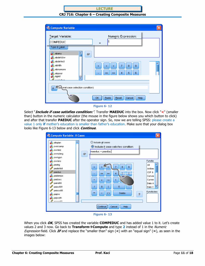
This new variable, that will once more (I can’t promise that it will be the last time, although I’ll try!) compare parents’ education, will be called COMPEDUC (i.e.: Compare Education). Don’t wait but just

type ―COMPEDUC‖ in the Target Variable field. Instead of entering the formula we now are used to in the Numeric Expression field, we will enter the new value, 1. You see… this is the reverse procedure of

the previous one, where we entered values by recoding the variable. With IF command you can enter the value directly in the box before creating the condition.

Well, the new variable name is entered, the first new value, 1, is also entered. What do we do? I thought

you’d never ask… This time click on the "If" button in the lower-left corner of the Compute Variable dialog box, as depicted on the Figure 6-12 below.

Transform Compute Variable IF

LECTURE



Figure 6- 12

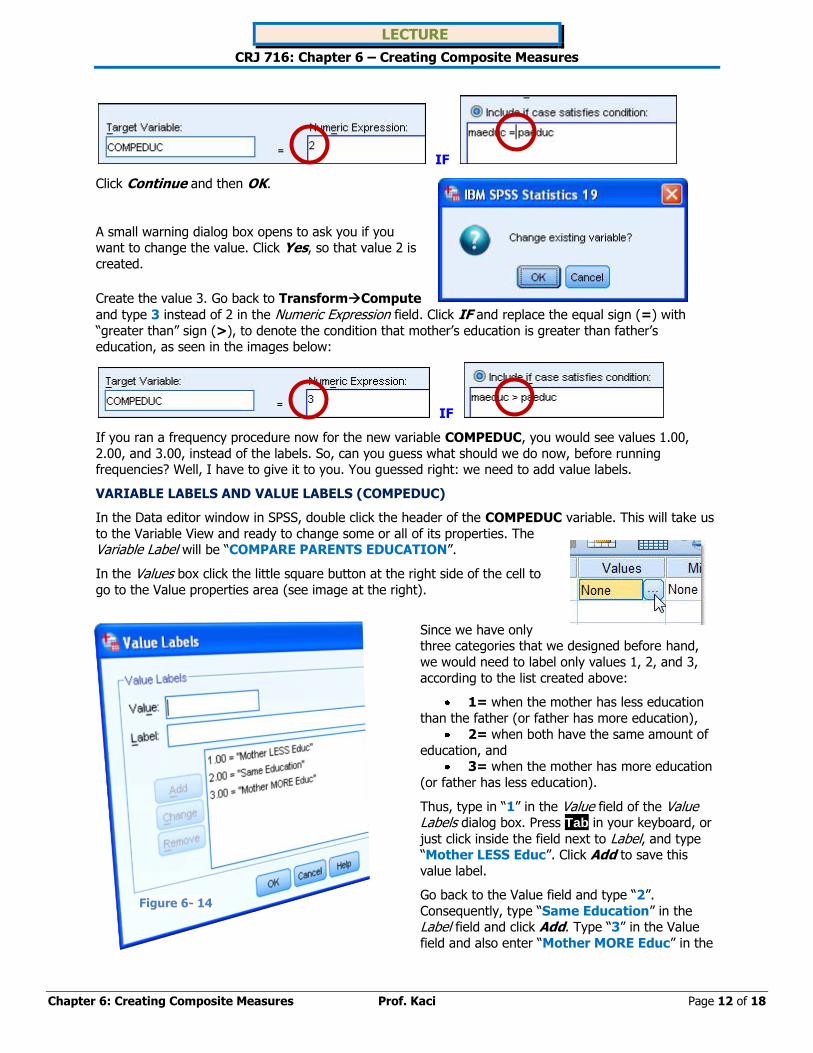
Select ―Include if case satisfies condition:‖. Transfer MAEDUC into the box. Now click "<" (smaller

than) button in the numeric calculator (the mouse in the figure below shows you which button to click) and after that transfer PAEDUC after the operator sign. So, now we are telling SPSS: please create a

value 1 only if mother’s education is smaller than father’s education. Make sure that your dialog box looks like Figure 6-13 below and click Continue.

Figure 6- 13

When you click OK, SPSS has created the variable COMPEDUC and has added value 1 to it. Let’s create values 2 and 3 now. Go back to TransformCompute and type 2 instead of 1 in the Numeric Expression field. Click IF and replace the ―smaller than‖ sign (<) with an ―equal sign‖ (=), as seen in the

images below:

LECTURE



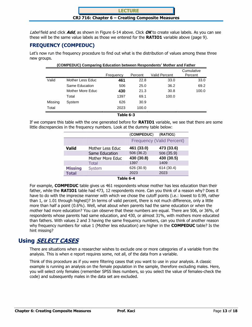
IF

Click Continue and then OK.

A small warning dialog box opens to ask you if you want to change the value. Click Yes, so that value 2 is

created.

Create the value 3. Go back to TransformCompute

and type 3 instead of 2 in the Numeric Expression field. Click IF and replace the equal sign (=) with

―greater than‖ sign (>), to denote the condition that mother’s education is greater than father’s education, as seen in the images below:

IF

If you ran a frequency procedure now for the new variable COMPEDUC, you would see values 1.00,

2.00, and 3.00, instead of the labels. So, can you guess what should we do now, before running frequencies? Well, I have to give it to you. You guessed right: we need to add value labels.

VARIABLE LABELS AND VALUE LABELS (COMPEDUC)

In the Data editor window in SPSS, double click the header of the COMPEDUC variable. This will take us

to the Variable View and ready to change some or all of its properties. The Variable Label will be ―COMPARE PARENTS EDUCATION‖.

In the Values box click the little square button at the right side of the cell to

go to the Value properties area (see image at the right).

Since we have only three categories that we designed before hand,

we would need to label only values 1, 2, and 3,

according to the list created above:

1= when the mother has less education

than the father (or father has more education),

2= when both have the same amount of

education, and 3= when the mother has more education

(or father has less education).

Thus, type in ―1‖ in the Value field of the Value Labels dialog box. Press Tab in your keyboard, or

just click inside the field next to Label, and type ―Mother LESS Educ‖. Click Add to save this

value label.

Go back to the Value field and type ―2‖.

Consequently, type ―Same Education‖ in the Label field and click Add. Type ―3‖ in the Value

field and also enter ―Mother MORE Educ‖ in the

Figure 6- 14

LECTURE



Label field and click Add, as shown in Figure 6-14 above. Click OK to create value labels. As you can see

these will be the same value labels as those we entered for the RATIO1 variable above (page 9).

FREQUENCY (COMPEDUC)

Let’s now run the frequency procedure to find out what is the distribution of values among these three new groups.

(COMPEDUC) Comparing Education between Respondents’ Mother and Father


Cumulative Percent

Valid Mother Less Educ 461 22.8 33.0 33.0

Same Education 506 25.0 36.2 69.2

Mother More Educ 430 21.3 30.8 100.0


Table 6-3

If we compare this table with the one generated before for RATIO1 variable, we see that there are some little discrepancies in the frequency numbers. Look at the dummy table below:

(COMPEDUC) (RATIO1)

Frequency (Valid Percent)

Valid Mother Less Educ 461 (33.0) 473 (33.6)

Same Education 506 (36.2) 506 (35.9) Mother More Educ 430 (30.8) 430 (30.5)

Total 1397 1409

Missing System 626 (30.9) 614 (30.4)

Total 2023 2023

Table 6-4

For example, COMPEDUC table gives us 461 respondents whose mother has less education than their father, while the RATIO1 table had 473, 12 respondents more. Can you think of a reason why? Does it

have to do with the imprecise manner with which we chose the cutoff points (i.e.: lowest to 0.99, rather

than 1, or 1.01 through highest)? In terms of valid percent, there is not much difference, only a little more than half a point (0.6%). Well, what about when parents had the same education or when the

mother had more education? You can observe that these numbers are equal. There are 506, or 36%, of respondents whose parents had same education, and 430, or almost 31%, with mothers more educated

than fathers. With values 2 and 3 having the same frequency numbers, can you think of another reason

why frequency numbers for value 1 (Mother less education) are higher in the COMPEDUC table? Is the hint missing?

Using SELECT CASES

There are situations when a researcher wishes to exclude one or more categories of a variable from the analysis. This is when e report requires some, not all, of the data from a variable.

Think of this procedure as if you were filtering cases that you want to use in your analysis. A classic

example is running an analysis on the female population in the sample, therefore excluding males. Here, you will select only females (remember SPSS likes numbers, so you select the value of females-check the

code) and subsequently males in the data set are excluded.

LECTURE



SELECT CASES — ONE GROUP AT A TIME

Suppose you wanted to find out how only females fared in their opinion towards death penalty. The first step in this analysis would be to go to the data set and select only the female population. The second

step is to run a frequency procedure to see if females oppose capital punishment more than they favor it.

To select cases, follow the procedure depicted in the diagram and Figure 6-15 below:

This will open the Select Cases dialog box. Click to check "If

condition is satisfied" radio button. This causes the button

"IF‖ below it to become active. Click on it, as shown in the

Figure 6-16 below, to launch "Select Cases: If" dialog box.

In the "Select Cases: If" dialog box, scroll

down to find variable Sex and transfer it

into the field to the right. Then click the = sign button, and then either press 2 (2 is the value for females) in your numeric keypad or click number 2 in the electronic keyboard in the dialog box. The

formula should be "sex = 2", signalizing that we want SPSS to select only females in this data set, which are coded with number 2 (males were coded as 1). Click Continue and then OK to select only females.

Figure 6-17

Data Select Cases

Figure 6-15

Figure 6-16

LECTURE



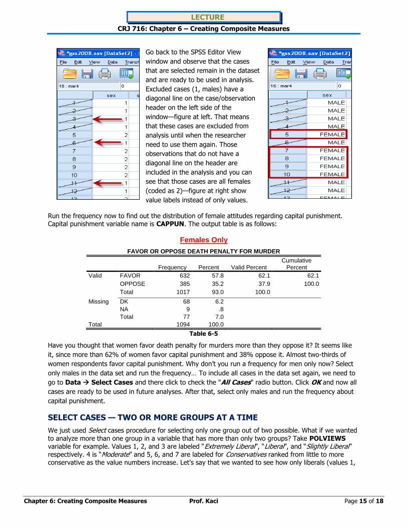
Go back to the SPSS Editor View

window and observe that the cases

that are selected remain in the dataset

and are ready to be used in analysis.

Excluded cases (1, males) have a

diagonal line on the case/observation

header on the left side of the

window—figure at left. That means

that these cases are excluded from

analysis until when the researcher

need to use them again. Those

observations that do not have a

diagonal line on the header are

included in the analysis and you can

see that those cases are all females

(coded as 2)—figure at right show

value labels instead of only values.

Run the frequency now to find out the distribution of female attitudes regarding capital punishment. Capital punishment variable name is CAPPUN. The output table is as follows:

Females Only

FAVOR OR OPPOSE DEATH PENALTY FOR MURDER


Cumulative Percent

Valid FAVOR 632 57.8 62.1 62.1

OPPOSE 385 35.2 37.9 100.0

Total 1017 93.0 100.0 Missing DK 68 6.2

NA 9 .8 Total 77 7.0

Total 1094 100.0

Table 6-5

Have you thought that women favor death penalty for murders more than they oppose it? It seems like

it, since more than 62% of women favor capital punishment and 38% oppose it. Almost two-thirds of

women respondents favor capital punishment. Why don’t you run a frequency for men only now? Select

only males in the data set and run the frequency… To include all cases in the data set again, we need to

go to Data Select Cases and there click to check the "All Cases" radio button. Click OK and now all

cases are ready to be used in future analyses. After that, select only males and run the frequency about

capital punishment.

SELECT CASES — TWO OR MORE GROUPS AT A TIME

We just used Select cases procedure for selecting only one group out of two possible. What if we wanted

to analyze more than one group in a variable that has more than only two groups? Take POLVIEWS variable for example. Values 1, 2, and 3 are labeled ―Extremely Liberal‖, ―Liberal‖, and ―Slightly Liberal‖ respectively. 4 is ―Moderate‖ and 5, 6, and 7 are labeled for Conservatives ranked from little to more conservative as the value numbers increase. Let’s say that we wanted to see how only liberals (values 1,

LECTURE



2, and 3) viewed capital punishment. In order to do this analysis we need to select only liberals, values 1,

2, and 3. Let us run the Select cases procedure once more:

In the Select Cases: If dialog box find the variable POLVIEWS and transfer it into the top box. Click ―=‖ sign and then type or click number 1 to select the first groups of the variable, ―Extremely Liberal‖, so that

the box reads ―polviews = 1‖. You should now expand your knowledge of the SPSS’s numeric electronic calculator and learn that the symbol "&" is used for the Boolean operator ―AND‖ and the symbol ―|‖ for

―OR‖. What we want is three categories, 1, 2 AND 3, so SPSS interprets this logic as ―cases for

POLVIEWS needed are 1 or 2 or 3. So, now click the symbol ―or‖ ("|") as depicted in Figure 6-18 below. Then transfer POLVIEWS again from the left list into the box, press equal (=) sign and then

press number 2. Now click the symbol ―or‖ ("|") and click on POLVIEWS again and bring it into the box for the third time, press =, and then 3. If the box contains: "polviews = 1 | polviews = 2 |

polviews = 3" as depicted in the figure below, you are fine.

Figure 6-18

Click Continue and then OK to select the cases.

If you now run a frequencies distribution for POLVIEWS variable you will get the following Output table:

Frequency Count for Liberals Only

Original Variable: THINK OF SELF AS LIBERAL OR CONSERVATIVE


Cumulative Percent

Valid EXTREMELY LIBERAL 69 13.0 13.0 13.0

LIBERAL 240 45.3 45.3 58.3

SLIGHTLY LIBERAL 221 41.7 41.7 100.0

Total 530 100.0 100.0

Table 6-6

This table only shows the three categories that we selected above, not all that make the variable. Other

groups are excluded.

Data Select Cases

LECTURE



Using SPLIT File There is another useful procedure, called Split File, which can give us output on different groups of a variable simultaneously. This option generates side by side tables for each category in a variable or can

create different output sections for each category. Let's stay within the Sex variable and split this data.

This will open the Split File dialog box—Figure 6-20. Click

to check Compare Groups radio button. Transfer the variable Sex into the Groups Based on field. You can

select Organize output by groups, which will give you a different Output. The first of these options—Compare Groups—puts corresponding pieces of output for the

different categories in one table, while the second option —Organize Output by groups—lists all the output in

different sections, derivatively different tables, below each other.

Click OK. The file is now split and ready for analysis.

Run the frequency for the CAPPUN variable, now that you have split the data into 2 groups that make

the SEX variable. If you selected Compare Groups, the Output window presents you with a big table

separated into two nested tables, one showing the frequencies for males and the other for females.

FAVOR OR OPPOSE DEATH PENALTY FOR MURDER

RESPONDENTS SEX Frequency Percent Valid Percent Cumulative Percent

MALE Valid FAVOR 631 67.9 71.3 71.3

OPPOSE 254 27.3 28.7 100.0

Total 885 95.3 100.0

Missing Total 44 4.7

Total 929 100.0

FEMALE Valid FAVOR 632 57.8 62.1 62.1

OPPOSE 385 35.2 37.9 100.0

Total 1017 93.0 100.0

Missing Total 77 7.0

Total 1094 100.0

Data Split file

Figure 6-19

Figure 6-20

LECTURE



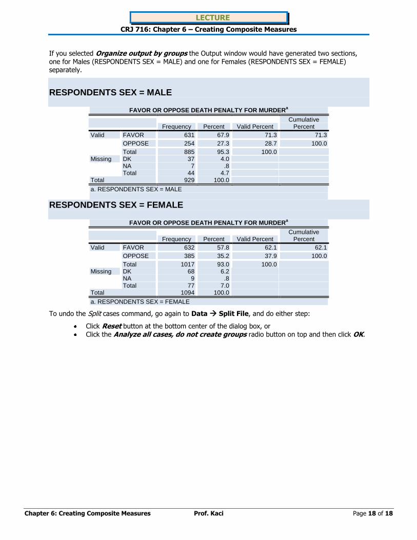
If you selected Organize output by groups the Output window would have generated two sections,

one for Males (RESPONDENTS SEX = MALE) and one for Females (RESPONDENTS SEX = FEMALE) separately.

RESPONDENTS SEX = MALE

FAVOR OR OPPOSE DEATH PENALTY FOR MURDERa


Cumulative Percent

Valid FAVOR 631 67.9 71.3 71.3

OPPOSE 254 27.3 28.7 100.0

Total 885 95.3 100.0

Missing DK 37 4.0

NA 7 .8

Total 44 4.7

Total 929 100.0

a. RESPONDENTS SEX = MALE

RESPONDENTS SEX = FEMALE

FAVOR OR OPPOSE DEATH PENALTY FOR MURDERa


Cumulative Percent

Valid FAVOR 632 57.8 62.1 62.1

OPPOSE 385 35.2 37.9 100.0

Total 1017 93.0 100.0

Missing DK 68 6.2

NA 9 .8

Total 77 7.0

Total 1094 100.0

a. RESPONDENTS SEX = FEMALE

To undo the Split cases command, go again to Data Split File, and do either step:

Click Reset button at the bottom center of the dialog box, or

Click the Analyze all cases, do not create groups radio button on top and then click OK.

Documents

Creating Composite Measures - John Jay College of …jjcweb.jjay.cuny.edu/...creating_composite_measures-compute-if.pdfLECTURE CRJ 716: Chapter 6 – Creating Composite Measures Chapter