Chapter 6 Creating Composite Measures - SAGE Publications · 75 UNIVARIATE ANALYSIS Chapter 6 Creating Composite Measures Now that you’ve had a chance to get familiar with univariate

75

UNIVARIATE ANALYSIS

Chapter 6 Creating Composite Measures

Now that you’ve had a chance to get familiar with univariate analysis, we’regoing to add a little more sophistication to that process. As you’re about to see, itis not necessary to limit your analysis to single measures of a variable. In thischapter, we’re going to create composite measures made up of multiple indica-tors of a single concept.

Why would a criminal justice researcher want to do that? Many of the keyconcepts in criminal justice are complex and can’t be indicated simply by theresponses to a single variable or by a single piece of information. To take a veryimportant example, how do we define crime among the most important conceptsin criminal justice? If we were trying to measure how much crime takes place ina state, it would not be enough just to look at any one type of serious crime. TheUniform Crime Reporting Program uses seven crime categories to establish a“crime index” to measure the trend and distribution of crime in the United States:murder and nonnegligent manslaughter, forcible rape, robbery, aggravatedassault, burglary, larceny and theft, and motor vehicle theft; the total crime indexis the sum of these offenses.

Take another example: You can explore the kinds of harm binge drinking hason nonbingeing students, also known as secondhand binge effects. Suppose thatyou want to determine how many residential students experience any of theseeffects or you want to find out how many of the effects (ranging from none to alleight) any of the students on a campus experienced.

In this chapter, we will explore how SPSS can help you create composite mea-sures such as a crime index or an index of secondhand binge effects. For purposesof this discussion, let’s look at attitudes toward abortion. Seven GSS items reflectpeople’s attitudes. You can ask SPSS to generate frequency tables for all sevenabortion variables from the “2004GSS.SAV” data set. (This exercise is also pre-sented on the Web site.) These tables on abortion suggest that attitudes towardabortion fall into three basic groups. A small minority of no more than 11% areopposed to abortion under any circumstance. We conclude this because 89%would support abortion if the woman’s life was seriously endangered. Anothergroup, a little under half of the sample population (48%), would support awoman’s free choice of abortion for any reason. The remainder of the sample pop-ulation would support abortion in only a few circumstances involving medicaldanger or rape.

06-Logio-45507.qxd 1/28/2008 4:15 PM Page 75

6.1 Using Crosstabs

To explore attitudes toward abortion in more depth, we need to use a new SPSScommand: “Crosstabs.” This command provides us with a cross-classification orcrosstabulation of people in terms of their answers to more than one question.The resulting table is sometimes called a crosstab or a contingency table, the lat-ter term indicating that the values of one variable are examined for how contin-gent they are on the values of another variable. Later in this book, we’ll explainhow to use crosstabs to test hypotheses about two or more variables when each ofthe variables is measured on the nominal or ordinal scale. Here we’ll use it to helpus understand how to combine variables into a composite measure. Let’s try asimple example.

The command pathway to this technique is “Analyze → Descriptive Statistics→ Crosstabs.” Work your way through those menu selections, and you shouldreach a window that looks like the following.

Because the logic of a crosstab will be clearer when we have an example tolook at, we ask that you follow these steps on faith, and we’ll explain it all in amoment.

Let’s analyze the relationship between the answers people gave to the ques-tion about whether a woman should be able to have an abortion if her health wasseriously endangered (ABHLTH) and if she was too poor to have more children.

In the “Crosstabs” window, click ABHLTH and then click the arrow point-ing toward the “Row(s)” field. Then click on ABPOOR and transfer it to the“Column(s)” field, producing the result shown next.

76 Univariate Analysis

06-Logio-45507.qxd 1/28/2008 4:15 PM Page 76

Once your window looks like this, click “OK.” After a few seconds, you willbe rewarded with the following data in your “Output” window.

Notice that the table demonstrates the logic of the command we asked you tomake. By specifying ABPOOR as the column variable, we have caused it to appearacross the top of the table with its attributes, “Yes” and “No,” representing the twocolumns of figures. ABHLTH, as the row variable, appears to the left of the table,and its attributes constitute the rows of the table.

More important, this table illustrates a logic that operates within the systemof attitudes people hold about abortion. First, we notice that 177 people say theywould support a woman’s decision to choose abortion if her health was seriouslyendangered and say they would support a woman’s choice of abortion if she waspoor and felt she couldn’t afford more children. At the opposite corner of the table,we find 36 people who would oppose abortion in both cases.

Chapter 6: Creating Composite Measures 77

06-Logio-45507.qxd 1/28/2008 4:15 PM Page 77

The table shows that 125 respondents said they would support the right tochoose if the woman’s health was seriously endangered but not on the basis ofpoverty. Notice that only one respondent would support abortion on the basis ofpoverty but deny it on the basis of threats to health. There are probably two elementsinvolved in this pattern. Threats to the woman’s life probably are seen as more seri-ous than the suffering presented by another mouth to feed in a poor family. At thesame time, few if any would blame a woman for ending a pregnancy that seriouslythreatened her health. However, some people blame the poor for their poverty andprobably would say that the woman in question should have avoided getting preg-nant because she knew that it would be hard for her to feed another child. As a con-sequence, then, 125 of the respondents oppose abortion under some circumstancesbut are willing to make an exception in the case of a threat to the woman’s health.

What are we to make of the one person who said he or she would approve anabortion for the poor but not for the woman whose life was threatened? Withoutruling out the possibility of some complex point of view that demands suchanswers, it is most likely that this respondent misunderstood one or both of thequestions. Fortunately, one is such a small number that this respondent will notseriously affect the analysis of this topic.

Additional information in the SPSS table will become more useful to us inlater analyses. For example, the rightmost column in the table tells us that a totalof 302 respondents with an opinion said they would approve an abortion for awoman whose health was seriously endangered, and 37 would not. The bottomrow of numbers in the table gives the breakdown regarding the other variable.

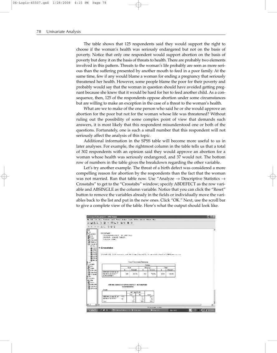
Let’s try another example. The threat of a birth defect was considered a morecompelling reason for abortion by the respondents than the fact that the womanwas not married. Run that table now. Use “Analyze → Descriptive Statistics →Crosstabs” to get to the “Crosstabs” window; specify ABDEFECT as the row vari-able and ABSINGLE as the column variable. Notice that you can click the “Reset”button to remove the variables already in the fields or individually move the vari-ables back to the list and put in the new ones. Click “OK.” Next, use the scroll barto give a complete view of the table. Here’s what the output should look like.


06-Logio-45507.qxd 1/28/2008 4:15 PM Page 78

This table presents a strikingly similar picture. We see that 166 respondents sup-port the woman’s right to choose in both situations, and 72 oppose abortion in bothinstances. Of those who would approve abortion in only one of the two situations,almost all of them (97) make the exception for the threat of birth defects. Only 4 respon-dents would allow abortion for a single woman but deny it in the case of birth defects.

We could continue examining tables like these, but the conclusion remains thesame: There are three major positions regarding abortion. One group approves it onthe basis of the woman’s choice, another group opposes it under all circumstances,and the rest approve abortion only in the case of medical complications or rape.

To explore attitudes toward abortion further, it will be useful for us to have ameasure of attitudes that is not limited to a single item. In particular, it might benice to have a single variable that captures the three groups we have been dis-cussing. We’re going to create two such composite measures in this chapter.

6.2 Combining Two Items in an Index

To begin, let’s create a simple index based on the two variables we just examined. Ouraim is to create a new measure—we’ll call it ABORT—made up of three scores: 2 forthose who approve of abortion if birth defects are likely and approve abortion for a sin-gle woman, 1 for those who approve of abortion in one circumstance (primarily birthdefects) but not the other, and 0 for those who disapprove of abortion in both cases.

To do this, let’s use the “Transform → Compute” command pathway. Thatwill bring up the following window.

To initiate our index construction, we need to create the new variable so thatSPSS will know where to put the results of our work. In the upper left corner of the“Compute Variable” window, click in the “Target Variable” field and type ABORT.

Notice that we’ve now begun a numeric expression that says “abort =,” tak-ing account of the equal sign already printed to the right of the “Target Variable”field. Our task from now on is to specify what ABORT equals by filling in the fieldtitled “Numeric Expression.” We’ll do this in several steps.

Begin by entering 0 in that field. You can do this in one of two ways. You cansimply type it in, or you can use the keypad in the center of the window. To usethe latter, simply click the “0” key.


06-Logio-45507.qxd 1/28/2008 4:15 PM Page 79

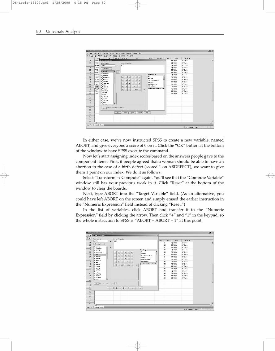
In either case, we’ve now instructed SPSS to create a new variable, namedABORT, and give everyone a score of 0 on it. Click the “OK” button at the bottomof the window to have SPSS execute the command.

Now let’s start assigning index scores based on the answers people gave to thecomponent items. First, if people agreed that a woman should be able to have anabortion in the case of a birth defect (scored 1 on ABDEFECT), we want to givethem 1 point on our index. We do it as follows.

Select “Transform → Compute” again. You’ll see that the “Compute Variable”window still has your previous work in it. Click “Reset” at the bottom of thewindow to clear the boards.

Next, type ABORT into the “Target Variable” field. (As an alternative, youcould have left ABORT on the screen and simply erased the earlier instruction inthe “Numeric Expression” field instead of clicking “Reset.”)

In the list of variables, click ABORT and transfer it to the “NumericExpression” field by clicking the arrow. Then click “+” and “1” in the keypad, sothe whole instruction to SPSS is “ABORT = ABORT + 1” at this point.


06-Logio-45507.qxd 1/28/2008 4:15 PM Page 80

Now we want SPSS to take this step only for respondents who agreed that awoman should be able to have an abortion in the case of a birth defect. To makethis specification, click the “If” button near the bottom of the window. Now youshould be looking at the following window:

This new window will help us specify our instruction to SPSS. Begin by clickingthe button “Include if case satisfies condition,” which will engage the variable list.

Transfer ABDEFECT to the open field and then add “= l.” using the keypad.Your screen should look like this:

We have now told SPSS that we want it to add a point to a person’s ABORTindex score only if the person’s score on ABDEFECT is 1.

To continue, click the “Continue” button, and you will be returned to the“Compute Variable” window, where you will see the following:


06-Logio-45507.qxd 1/28/2008 4:15 PM Page 81

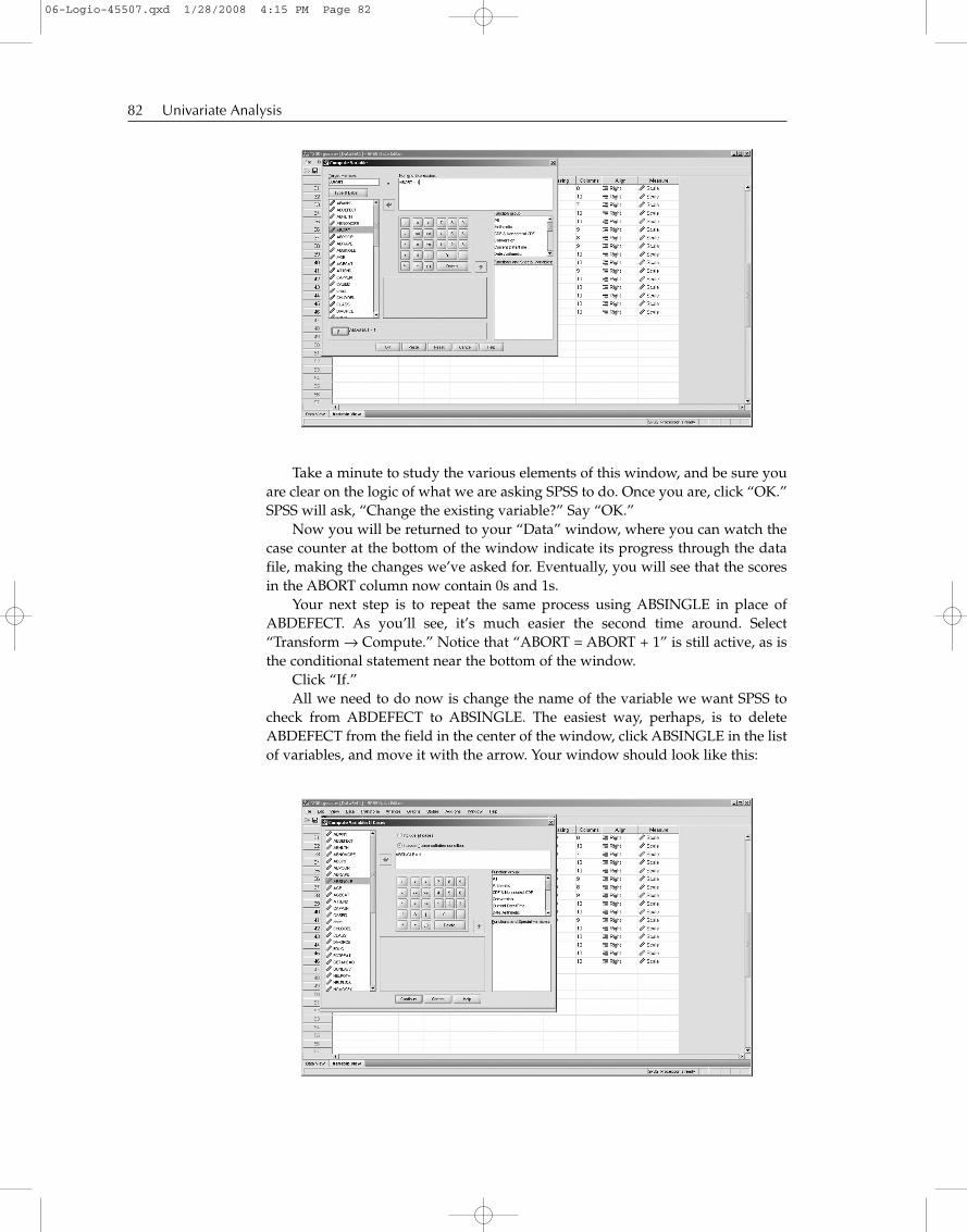
Take a minute to study the various elements of this window, and be sure youare clear on the logic of what we are asking SPSS to do. Once you are, click “OK.”SPSS will ask, “Change the existing variable?” Say “OK.”

Now you will be returned to your “Data” window, where you can watch thecase counter at the bottom of the window indicate its progress through the datafile, making the changes we’ve asked for. Eventually, you will see that the scoresin the ABORT column now contain 0s and 1s.

Your next step is to repeat the same process using ABSINGLE in place ofABDEFECT. As you’ll see, it’s much easier the second time around. Select“Transform → Compute.” Notice that “ABORT = ABORT + 1” is still active, as isthe conditional statement near the bottom of the window.

Click “If.”All we need to do now is change the name of the variable we want SPSS to

check from ABDEFECT to ABSINGLE. The easiest way, perhaps, is to deleteABDEFECT from the field in the center of the window, click ABSINGLE in the listof variables, and move it with the arrow. Your window should look like this:


06-Logio-45507.qxd 1/28/2008 4:15 PM Page 82

Click “Continue,” then click “OK.” When asked whether you want to changethe variable, click “OK.”

Our index is nearly complete now. However, we must take account of thepeople who did not answer either or both of the questions included in the index,people scored as “missing data.”

Recall that so far, we gave everyone a score of 0 to begin with, and thenrespondents who scored 1 on ABDEFECT or ABSINGLE were given additionalpoints. Those who had missing data on the two items are still scored 0 on ourindex. Thus they look as though they are strongly opposed to abortion, whereasthey were actually never asked about it.

To complete our index, then, we must create a missing data code for ABORTand assign that code to the appropriate cases. Let’s use –1 because that has nomeaning on the index.

Return to “Transform → Compute.” Put –1 into the “Numeric Expression”field and click “If” to tell SPSS when we want the –1 code assigned on ABORT.

Instead of specifying a numeric value for ABDEFECT and ABSINGLE, we aregoing to use the list of functions found on the right side of the window. Scrolldown the list until you find “Missing Values.” Select it and then choose from thelist below called “Functions and Special Values.” We want to choose the “Missing”option. When we do, the description of what that includes is to the left. Thisexplains that any respondent who is system- or user-missing (meaning that theydidn’t answer the question or they weren’t asked the question) will be includedamong the missing.


06-Logio-45507.qxd 1/28/2008 4:15 PM Page 83

Notice that the expression now has a highlighted question mark. Replace thehighlighted question mark this time by selecting and transferring the variablename ABDEFECT.

We have now created the following instruction for SPSS: If a person has amissing data code on ABDEFECT, we want that person scored as –1 on the indexABORT. Once you understand the logic of this instruction, click “Continue,” thenclick “OK” to execute the instruction.

Now repeat the same procedure using ABSINGLE where you simply replaceABDEFECT with ABSINGLE.

Our index is almost complete now, but we want to make two modifications to it.In the “Variable View” of the “Data Editor” window, find and select the new

variable, ABORT, at the bottom. Once you’ve done that, select the box in the“Missing” column for the new variable.

Notice that the index currently has “None” listed as missing. Click on thesmall gray box. Click “Discrete missing values” and type –1 into the first boxunderneath it. This tells SPSS that we have assigned that numeric score for allcases that got no index score on ABORT.


06-Logio-45507.qxd 1/28/2008 4:15 PM Page 84

Once you are satisfied with the instruction, click “OK” to return to the“Variable View” window.

As we did the last time we were here, we want to set the number of decimalplaces to 0. Click on the box in the “Decimals” column and use the arrows to bringthe 2 to a 0. We will not enter any labels at this point. Just go back to the “DataView” window, where you will see ABORT with its codes of –1, 0, 1, and 2.

Now let’s see whether all this really accomplished what we set out to do. Usethe “Frequencies” command to find out. Run the frequency distribution ofABORT, and you should see this table on your screen now:

If you compare the index scores in this table with the crosstabs of the twocomponent variables, you’ll see a logical correspondence. In the earlier table, 72people disapproved of abortion under both of the specified conditions; here wefind that 72 people scored 0 on the index. And whereas we found that 97 people


06-Logio-45507.qxd 1/28/2008 4:15 PM Page 85

would approve abortion for birth defects but not for a single woman and 4 hadthe reverse view, the index shows 101 people (97 + 4) with a score of 1. Finally, the166 people who approved of abortion in both cases are now scored 2 on the index.Notice also the 861 people who were excluded on the basis of missing data.

Congratulations! You’ve just created a composite index. We realize you maystill be wondering why that’s such good news. After all, it wasn’t your idea tocreate the thing in the first place.

6.3 Checking to See How the Index Works

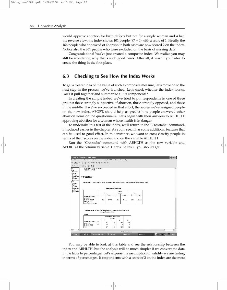
To get a clearer idea of the value of such a composite measure, let’s move on to thenext step in the process we’ve launched. Let’s check whether the index works.Does it pull together and summarize all its components?

In creating the simple index, we’ve tried to put respondents in one of threegroups: those strongly supportive of abortion, those strongly opposed, and thosein the middle. If we’ve succeeded in that effort, the scores we’ve assigned peopleon the new index, ABORT, should help us predict how people answered otherabortion items on the questionnaire. Let’s begin with their answers to ABHLTH:approving abortion for a woman whose health is in danger.

To undertake this test of the index, we’ll return to the “Crosstabs” command,introduced earlier in the chapter. As you’ll see, it has some additional features thatcan be used to good effect. In this instance, we want to cross-classify people interms of their scores on the index and on the variable ABHLTH.

Run the “Crosstabs” command with ABHLTH as the row variable andABORT as the column variable. Here’s the result you should get:

You may be able to look at this table and see the relationship between theindex and ABHLTH, but the analysis will be much simpler if we convert the datain the table to percentages. Let’s express the assumption of validity we are testingin terms of percentages. If respondents with a score of 2 on the index are the most


06-Logio-45507.qxd 1/28/2008 4:15 PM Page 86

supportive of abortion, we should expect to find a higher percentage of themapproving of abortion in the case of the woman’s health being endangered thanwould be found among the other groups. Those scored 0 on the index, by contrast,should be the least likely—the smallest percentage—to approve of abortion basedon the woman’s health.

Looking first at those with a score of 0, in the leftmost column of the table, wewould calculate the percentage as follows. Of the 67 people scored 0, we see that37 approved of abortion in the case of ABHLTH. Dividing 37 by 67 indicates thatthese 37 people are 55.22% of the total 67. Looking to those scored 2, in the right-most column, we find that the 163 who approve represent 98.79% of the 165 withthat score. These two percentages support the assumption we are making aboutthe index; it does seem to be working.

Fortunately, SPSS can be instructed to calculate these percentages for us. Infact, we are going to be looking at percentage tables for the most part in the restof this book. Go back to the “Crosstabs” window. Your previous request shouldstill be in the appropriate fields. Notice a button at the bottom of this windowmarked “Cells.” Click it. This will take you to a new window as shown here:

Notice that you can choose to have SPSS calculate percentages for you in oneof three ways: either down the columns, across the rows, or total percentages.Click “Columns” and work your way back through the “OKs” to have SPSS runthe table for you. The result should look like the following:


06-Logio-45507.qxd 1/28/2008 4:15 PM Page 87

Take a moment to examine the logic of this table. For each score on the index,we have calculated the percentage of respondents saying they favor or oppose awoman’s right to an abortion if her health is seriously endangered. It is as thoughwe have limited our attention to one of the index score groups (e.g., those scored0) and described them in terms of their attitudes on the abortion item; thenwe have repeated the process for each of the index score groups. Once we’vedescribed each of the subgroups, we can compare them.

When you have created a table with the percentages totaling to 100 down eachcolumn, the proper way to read the table is across the rows. Rounding off the per-centages to simplify matters, we would note, in this case, that 55% of those scored0 on the index, 96% of those scored 1 on the index, and 99% of those scored 2 onthe index said they would approve of abortion if the woman’s health were seri-ously endangered. This table supports our assumption that the index measureslevels of support for a woman’s freedom to choose abortion.

Now let’s check the index using the abortion variables not included in theindex itself. Repeat the “Crosstabs” command, substituting the four other abor-tion items—ABNOMORE, ABRAPE, ABPOOR, and ABANY—for ABHLTH.

Run the “Crosstabs” command now and see what results you get. Look ateach of the four tables and see what they say about the ability of the index to mea-sure attitudes toward abortion. Here is an abbreviated table format that you mightwant to construct from the results of that command. SPSS doesn’t create a tablelike this, but it’s a useful format for presenting data in a research report.

Percentage of respondents who approve of abortion under various circumstances:

Abortion Index

Circumstance 0 1 2

When the woman was raped 27 86 99The couple can’t afford more children 0 27 92The couple doesn’t want more children 1 24 92The woman wants an abortion 1 15 92


06-Logio-45507.qxd 1/28/2008 4:15 PM Page 88

Whereas the earlier table showed the percentages who approved and disap-proved of abortion in specific situations, this table presents only those whoapproved. The first entry in the table, for example, indicates that 27% of thosescored 0 on the index would approve of abortion for a woman who was raped. Ofthose scored 1 on the index, 86% approved of abortion for this reason, and 99% ofthose scored 2 approved.

As you can see, the index accurately predicts differences in responses to eachof the other abortion items. In each case, those with higher scores on the index aremore likely to support abortion under the specified circumstances than those withlower scores on the index.

By building this composite index, we’ve created a more sophisticated measureof attitudes toward abortion. Whereas each of the individual items allows only forapproval or disapproval of abortion under various circumstances, this indexreflects three positions on the issue: unconditional disapproval (0), conditionalapproval (1), and unconditional approval (2).

6.4 Creating a More Complex Index With Count

This first index was created from only two of the abortion items, but we couldeasily create a more elaborate index, using more items. To illustrate, let’s useall the items except for ABANY (supporting a woman’s unrestricted choice).Although we could create this new index by following the same procedures asbefore, there is also a shortcut that we can use when we want to score severalitems the same way in creating the index. Suppose that we want to create alarger index by giving people one point for agreeing to an abortion in each ofthe six special circumstances. From the “Transform” menu, select “Count.”Then select “Count Values within Cases.” This will present you with the follow-ing window:

In creating our new index, we will once more need to deal with the problemof missing values. In using “Count,” we are going to handle that matter somewhat


06-Logio-45507.qxd 1/28/2008 4:15 PM Page 89

differently from before. Specifically, we are going to begin by creating a variablethat tells us whether people had missing values on any of the six items we areexamining. To do this, we’ll create a variable called MISS. Type that name in the“Target Variable” field.

Next, we want to specify the items to be considered in creating MISS. Transferthe following variable names to the “Variables” field: ABDEFECT, ABHLTH,ABNOMORE, ABPOOR, ABRAPE, and ABSINGLE. You can do this by selectinga variable in the list on the left side of the window and clicking the arrow point-ing to the “Variables” field, or you can simply double-click a variable name.Where several variables are together in the list, you can click and drag your cur-sor down the several names, selecting them all, and then click the arrow. Becareful, though. The ABORT variable we just created is in the list, but we do notwant to transfer it to the “Variables” field. Only the six variables (ABDEFECT,ABHLTH, ABNOMORE, ABPOOR, ABRAPE, and ABSINGLE) should be listed.

Having selected the variables to be counted, click “Define Values.”The left side of the window offers several options for counting, but we want

to use the simplest: a single value. Click the button beside “System- or user-missing.” Click the “Add” button to transfer the value to the “Values to Count”field. “MISSING” will now appear in that space. Click “Continue” to return to the“Count Occurrences” window.

Click “OK” to launch the procedure. Once SPSS has completed the procedure,you will find yourself looking at the “Output” window. Switch over to the “Data”window with the “Data View” tab forward and scroll to the end to see the last vari-able. There will be a new variable called MISS, with scores ranging from 0 to 6,indicating the number of missing values people had on the six items.

Now we are ready to create our new abortion index. Select “Count Valueswithin Cases” from the “Transform menu” again. Notice that our earlier specifica-tions are still there; these will be very useful to us.


06-Logio-45507.qxd 1/28/2008 4:15 PM Page 90

Replace MISS with ABINDEX in the “Target Variable” field. Click “DefineValues.” In the “Values to Count” window, you’ll notice that MISSING is stillshowing in the specification field. Click it to select it. Then click “Remove.” Nowthe field is empty.

Click the first option on the left, “Value,” and type “1” in the field beside it.Click “Add” to transfer the value to the appropriate field.

Then click “Continue.” Because we left the six variable names in the“Numeric Values” field, we have now told SPSS to count the number of times aperson had a score of 1 on any of those six items.

Before having SPSS do its counting, however, we can use the MISS index wecreated a moment ago.

Click “If.” In the “If Cases” window, click “Include if case satisfies condition.”Notice that the list of variables on the left is activated by that. You can either find


06-Logio-45507.qxd 1/28/2008 4:15 PM Page 91

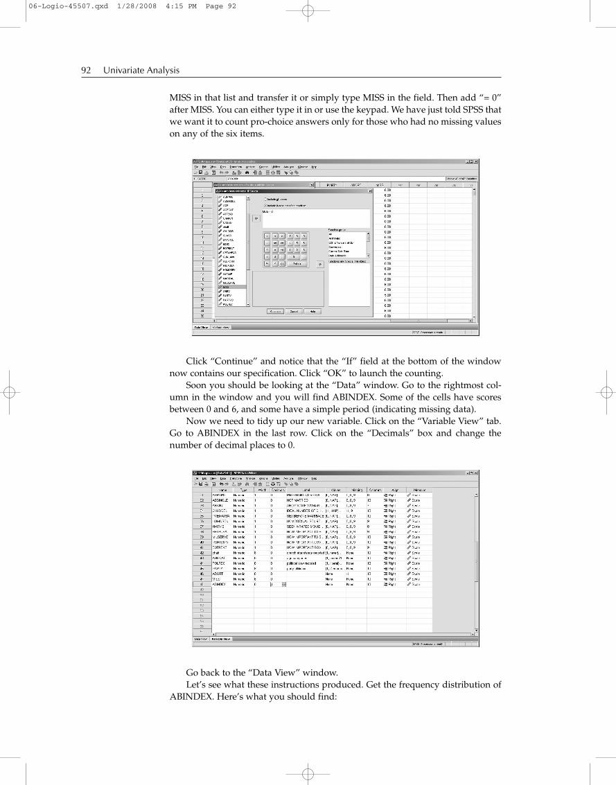
MISS in that list and transfer it or simply type MISS in the field. Then add “= 0”after MISS. You can either type it in or use the keypad. We have just told SPSS thatwe want it to count pro-choice answers only for those who had no missing valueson any of the six items.

Click “Continue” and notice that the “If” field at the bottom of the windownow contains our specification. Click “OK” to launch the counting.

Soon you should be looking at the “Data” window. Go to the rightmost col-umn in the window and you will find ABINDEX. Some of the cells have scoresbetween 0 and 6, and some have a simple period (indicating missing data).

Now we need to tidy up our new variable. Click on the “Variable View” tab.Go to ABINDEX in the last row. Click on the “Decimals” box and change thenumber of decimal places to 0.

Go back to the “Data View” window.Let’s see what these instructions produced. Get the frequency distribution of

ABINDEX. Here’s what you should find:


06-Logio-45507.qxd 1/28/2008 4:15 PM Page 92

This table shows the distribution of scores on the new index, ABINDEX. (Usethe scroll bar on the right-hand side of the window to move the output text up anddown so that you can see whatever output you want to look at.) As you can see,there are 139 people, more than two-fifths of those with opinions, who supportabortion in all the specified circumstances. A total of 28 disapprove of abortion inany of those circumstances. The rest are spread out according to the number ofconditions they feel would warrant abortion.

For validation purposes this time, we have only one item not included in theindex itself: ABANY. Let’s see how well the index predicts respondents’ approvalof a woman’s unrestricted choice of abortion.

Run the “Crosstabs” procedure, specifying ABANY as the row variable,ABINDEX as the column index, and cells to be percentaged by column.

Looking at the SPSS output, using the scroll bars if necessary, we can see thatanswers to ABANY are closely related to scores on ABINDEX. Of those with 0 on


06-Logio-45507.qxd 1/28/2008 4:15 PM Page 93

the index, no one said a woman had a right to an abortion for any reason. No onewho scored 1 on ABINDEX favored a woman’s right to an abortion for any reasoneither. For the scores 2 through 6, the percentage continues increasing across theindex until we find that 98.6% of those scored 6 on the index say a woman hasthe unconditional right to an abortion. (You may have to scroll over to the right tosee the entire table with all the columns.)

Once again, we find that the index works well. This means that if we want toanalyze peoples’ attitudes toward abortion further (and we will), we have thechoice of using a single item to represent those attitudes or using a compositemeasure. If we’ve constructed the index well, it should be superior to any one ofits component parts, providing much more information about a particular topic.Moreover, we’ve seen that we can create such an index in different ways.

6.5 Creating the FBI Crime Index

To take a very different example of creating a composite index, we will follow thesimple steps necessary to create perhaps the most famous composite index incriminal justice. To do this, we’ll use another file from the Web site, so give SPSSthe commands necessary to open the “JUSTICE.SAV” file. Once you’ve openedthis file, follow this chapter’s instructions to combine the crimes mentioned at thebeginning of this chapter into an overall index. This index will be a simple addi-tion of the component crimes into an overall sum of those crimes for each state. Itis a simple index because none of the variables has any missing data. The indexwill include the following items:

� Murder and nonnegligent manslaughter� Forcible rape� Robbery� Aggravated assault� Burglary� Larceny and theft� Motor vehicle theft

6.6 Secondhand Binge Effects: Creating an Index

How about a real challenge? A final example of index construction asks you tobegin by opening the “BINGE.SAV” file. Concentrate your efforts on constructingan index that combines the survey items in which a student reports having expe-rienced some problem as the result of the drinking of some other student. Justas “secondhand smoke” means that someone else’s smoking causes a nonsmokerto suffer some of the same ill effects as a smoker, “secondhand binge” means thatnonbingeing students suffer those effects. This example is a bit more challengingthan the last one. It will involve several steps. First, the index should include onlynonbingeing students. Next, because you want to examine the impact of bingedrinking on students who live on campus, make the index include only studentswho live in dormitories, fraternities, or sororities. Finally, include the followingitems from the College Alcohol Study, asking whether a student experienced eachof these:


06-Logio-45507.qxd 1/28/2008 4:15 PM Page 94

� Been insulted or humiliated� Had a serious argument or quarrel� Been pushed, hit, or assaulted� Had your property damaged� Had to “baby-sit” or take care of another student who drank too much� Had your studying or sleep interrupted� Experienced an unwanted sexual advance� Been a victim of sexual assault or date rape

You can create an index that should count up the number of secondhandbinge effects that a student experienced. Because there are eight items, this indexcan vary from 0 to 8. Remember to construct this index variable taking missingvalues into account.

6.7 Summary

In this chapter, we’ve seen that it is often possible to measure criminal justice andother social scientific concepts in a number of ways. Sometimes the data set con-tains a single item that does the job nicely. Measuring gender by asking people fortheir gender is a good example.

In other cases, the mental images that constitute our concepts (e.g., attitudesabout abortion, serious crime in a state, or the experience of secondhand bingeeffects) are varied and ambiguous. Typically, no single item in a data set providesa complete representation of what we have in mind. Often we can resolve thisproblem by combining two or more indicators of the concept into a compositeindex. As we’ve seen, SPSS offers the tools necessary for such data transformations.

If you continue your studies in criminal justice research, you will discovermany more sophisticated techniques for creating composite measures. However,the simple indexing techniques you have learned in this chapter will serve youwell in the analyses that lie ahead.

Key Terms


composite measurescontingency tablecrosstabcrosstabulationmultiple indicators

Student Study Site

Log on to the Web-based student study site at http://www.sagepub.com/logiostudy for access tothe data sets referred to in the text and additional study resources.

06-Logio-45507.qxd 1/28/2008 4:15 PM Page 95

06-Logio-45507.qxd 1/28/2008 4:15 PM Page 96

Documents

Chapter 6 Creating Composite Measures - SAGE Publications · 75 UNIVARIATE ANALYSIS Chapter 6 Creating Composite Measures Now that you’ve had a chance to get familiar with univariate