Abstract—To increase the lifting capacity and minimize the

cost and time for building a ship and offshore structure, block

lifting with multi-cranes becomes more and more danger. In

this paper, therefore, dynamic response analysis of the

multi-cranes is performed for block lifting operation. By this

simulation, one can confirm the dynamic effects, such as

dynamic motion and load, to prevent fatal accidents during the

multi-crane operation. The crane system consists of several

bodies. These bodies are connected with various types of joints

and wire rope. To carry out the dynamic simulation, therefore,

the crane system is modeled as a multi-body system. There are

several types of crane, such as a goliath crane, jib crane, and

floating crane, etc. Among them, the floating crane is operated

on the sea water. Therefore the hydrostatic force and linearized

hydrodynamic force are considered as the external forces acting

on the floating crane. Using the dynamics simulation program

developed in this paper, a dynamic response simulation of

several cases of block lifting with multi-cranes are carried out,

and the simulation results are validated by comparing them

with the measured data from the shipyard. Moreover, the

simulation results can be applied to the structural analysis for

evaluate the dynamic effects on the block.

Index Terms—Dynamic simulation, modeling and

simulation, multi-body system, large scale manufacturing,

structural analysis.

I. INTRODUCTION

Recently, the shipyard has been manufacturing the

offshore structure blocks as large as possible for minimize

the building cost and time. But weight of these blocks often

exceeds the lifting capability of the crane. Thus to solve this

problem, the shipyard has started to use multiple cranes to lift

the heavy loads.

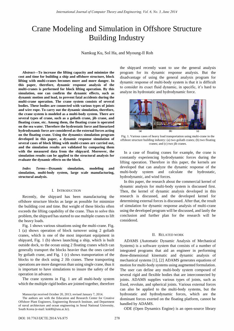
Fig. 1 shows various situations using the multi-crane. Fig.

1 (a) shows operation of block turnover using 2 goliath

cranes, which is one of the most important equipment in

shipyard, Fig. 1 (b) shows launching a ship, which is built

outside dock, to the ocean using 2 floating cranes which can

generally transport the blocks heavier than the ones carried

by goliath crane, and Fig. 1 (c) shows transportation of the

blocks to the dock using 2 Jib cranes. These transporting

operations are more dangerous than using single crane, thus it

is important to have simulations to insure the safety of the

operation in advance.

The crane systems in Fig. 1 are all multi-body system

which the multiple rigid bodies are jointed together, therefore

Manuscript received October 20, 2013; revised January 7, 2014.

The authors are with the Education and Research Center for Creative

Offshore Plant Engineers, Engineering Research Institute, and Department

of naval architecture and ocean engineering in Seoul National University,

South Korea (e-mail: knk80@snu.ac.kr).

the shipyard recently want to use the general analysis

program for its dynamic response analysis. But the

disadvantage of using the general analysis program for

dynamic response of multi-body system is that it is difficult

to consider its exact fluid dynamic, in specific, it’s hard to

analyze its hydrostatic and hydrodynamic force.

Fig. 1. Various cases of heavy load transportation using multi-crane in the

offshore structure building industry: (a) two goliath cranes; (b) two floating

cranes; and (c) two jib cranes.

In a case of floating cranes for example, the crane is

constantly experiencing hydrodynamic forces during the

lifting operation. Therefore in this paper, the kernels are

developed that can analyze the dynamic response of the

multi-body system and calculate the hydrostatic,

hydrodynamic, and wind forces.

In this paper, the research about the commercial kernel of

dynamic analysis for multi-body system is discussed first.

Then, the kernel of dynamic analysis developed in this

research is discussed, and the developed kernel for

determining external forces is discussed. After that, the result

of simulation for dynamic response analysis of multi-crane

using the developed program will be discussed, and lastly the

conclusion and further plan for the research will be

considered.

II. RELATED WORK

ADAMS (Automatic Dynamic Analysis of Mechanical

Systems) is a software system that consists of a number of

integrated programs that aid an engineer in performing

three-dimensional kinematic and dynamic analysis of

mechanical systems [1], [2] ADAMS generates equations of

motion for multi-body systems using augmented formulation.

The user can define any multi-body system composed of

several rigid and flexible bodies that are interconnected by

joints. ADAMS supplies various types of joints, such as

fixed, revolute, and spherical joints. Various external forces

can also be applied to the multi-body systems, but the

hydrostatic and hydrodynamic forces, which are the

dominant forces exerted on the floating platform, cannot be

handled by ADAMS.

ODE (Open Dynamics Engine) is an open-source library

Crane Modeling and Simulation in Offshore Structure

Building Industry

Namkug Ku, Sol Ha, and Myoung-Il Roh

International Journal of Computer Theory and Engineering, Vol. 6, No. 3, June 2014

278DOI: 10.7763/IJCTE.2014.V6.875

for simulating multi-body dynamics [3]. Similar to ADAMS,

ODE derives equations of motion for multi-body systems

using augmented formulation. ODE can treat only rigid

bodies, however, not flexible bodies. Moreover, ODE cannot

handle hydrostatic and hydrodynamic forces.

RecurDyn [4] is a three-dimensional simulation software

that combines dynamic response analysis and finite element

analysis tools for multi-body systems. It is 2 to 20 times faster

than other dynamic solutions because of its advanced fully

recursive formulation. Various joints and external forces can

also be applied to the multi-body systems, but RecurDyn

cannot handle hydrostatic and hydrodynamic forces.

This study presents the development of a dynamics kernel

for the dynamic analysis of offshore structures such as

semi-submersible drilling rig or drill ship. The equations of

motion for multi-body systems were derived using recursive

formulation. Moreover, the external force calculation module

can generate hydrostatic force by considering the nonlinear

effects and the linearized hydrodynamic force as external

forces.

It is possible to interface these general programs with

hydrodynamics using user-subroutine. For example,

Jonkman developed a module called “HydroDyn” for

calculating hydrodynamic force in time domain and interface

it with other program [5]. For calculating hydrodynamic

force in time domain, Jonkman transforms the analysis

results from “WAMIT”, which is a commercial program for

calculating hydrodynamic force in frequency domain, into

time domain using Cummins equation. In other words, the

analysis results from “WAMT” are required to use

“Hydrodyn”. In this research, to make the developed kernel

independent from any other programs, 3D Rankine panel

method is applied for direct calculation of hydrodynamic

force in time domain. To interface 3D Rankine panel method

with the existing programs of dynamic response analysis for

multi-body, input of hydrodynamic force is not enough. To

increase numerical stability, it is required to modify the mass

and inertia of the floating body using added mass. Therefore

it is not easy to interface with other commercial programs.

Moreover, as mentioned above, to make the developed kernel

independent from any other programs, the functions for

analyzing dynamic response of multi-body and calculating

hydrostatic and dynamic force are integrated together. Table

I shows the features of the different dynamics kernels that

were compared in this study.

TABLE I: COMPARISON OF THE FEATURES OF THE DEVELOPED DYNAMICS

KERNEL IN THIS STUDY WITH COMMERCIAL DYNAMICS KERNEL

This study ADAMS ODE RecurDyn

Multi-body

formulation

Recursive

formulation

Augmented

formulation

Augmented

formulation

Recursive

formulation

Various

joints Ｏ Ｏ Ｏ Ｏ

Flexible

body X Ｏ X Ｏ

Hydrostatic

force Ｏ Δ Δ Δ

Linearized

hydrodyna

mic force

Ｏ Δ Δ Δ

*(Ｏ: Supported; Δ: Can be only interfaced by the developer of the dynamics

kernel)

III. DEVELOPMENT OF KERNEL OF DYNAMIC ANALYSIS FOR

MULTI-BODY SYSTEM

The kernel of dynamic analysis is developed for the

multi-body system. In this section, the recursive formulation

applied for the construction of kinematic equation of

multi-body system is explained.

A. Forward and Inverse Dynamics

The dynamics of a rigid-body system are described by its

equation of motion, which specifies the relationship between

the forces that act on the system and the accelerations they

produce. The main concern in this section is the algorithms

for the following two particular calculations.

Forward dynamics: The calculation of the acceleration

response of a given rigid-body system to a given applied

force

Inverse dynamics: The calculation of the force that must

be applied to a given rigid-body system to produce a

given acceleration response

Forward dynamics is used mainly in simulation. Inverse

dynamics will be explained first, however, since it is easier

than forward dynamics in the manner of the explanation of

the recursive formulation [6].

B. Inverse Dynamics of Recursive Formulation

The equations of motion for each body of the multi-body

system based on recursive formulation can be summarized as

following.

1 1ˆ ˆi

i i i i iq v X v S (1)

1 1ˆ ˆ ˆi

i i i i i i i i i iq q q a X a S S v S (2)

*ˆ ˆ ˆˆ ˆ ˆB

i i i i i i f I a v I v (3)

*

1 1ˆ ˆ ˆ ˆB i ext

i i i i i f f X f f (4)

ˆT

i i i S f - (5)

In here, ˆiv is velocity vector(6 elements) of body ©, ˆ

ia is

acceleration vector(6 elements) of body ©, iq is generalized

coordinate(joint value), iS is velocity transformation matrix,

iI is mass and mass moment of inertia of body ©, ˆ B

if is

resultant force exerted on body ©, ˆext

if is external force

exerted on body ©, ˆif is force across the joint ©, and i is

force generated by joint © (generalized force). In inverse

dynamics, since the positions iq , velocities iq , and

accelerations i

q of generalized coordinates are given, the

velocities ˆiv and accelerations ˆ

ia of each body can be

computed. Furthermore, the forces ˆif and the generalized

forces i , which should be exerted on each link, can be also

computed in a recursive fashion [6], [7].

For example, the equations of motion for the three-link

multi-body system can be formulated as shown in Fig. 2.

International Journal of Computer Theory and Engineering, Vol. 6, No. 3, June 2014

279

1

1 0 0 1 1ˆ ˆ q v X v S

*

1 1 1 1 1 1ˆ ˆ ˆˆ ˆ ˆB f I a v I v

1 1 1ˆT S f

1

1 0 0 1 1 1 1 1 1 1ˆ ˆ ˆq q q a X a S S v S

1 *

1 1 2 2 1ˆ ˆ ˆ ˆB ext f f X f f

(1-a)

(1-b)

(1-c)

(1-d)

(1-e)

2 1 1 2 2ˆ ˆi q v X v S

*

2 2 2 2 2 2ˆ ˆ ˆˆ ˆ ˆB f I a v I v

2 2 2ˆT S f

2

2 1 1 2 2 2 2 2 2 2ˆ ˆ ˆq q q a X a S S v S

2 *

2 2 3 3 2ˆ ˆ ˆ ˆB ext f f X f f

(2-a)

(2-b)

(2-c)

(2-d)

(2-e)

3

3 2 2 3 3ˆ ˆ q v X v S

*

3 3 3 3 3 3ˆ ˆ ˆˆ ˆ ˆB f I a v I v

3 3 3ˆT S f

3

3 2 2 3 3 3 3 3 3 3ˆ ˆ ˆq q q a X a S S v S

3 *

3 3 4 4 3ˆ ˆ ˆ ˆB ext f f X f f

(3-a)

(3-b)

(3-c)

(3-d)

(3-e)

Equations of motion for link 1

Equations of motion for link 2

Equations of motion for link 3

E

ny

nx

Base

1q

2q

3q

1 2 3 1 2 3

1 2 3

, , , , , ,

, ,

q q q q q q

q q q

1 2 3, ,

1

2

3

Given:

Fine:

Fig. 2. Example of an inverse dynamics problem: three-link multi-body

system.

1) The velocity of link 1, 1v , can be determined using

(1-a), since the velocity of the base, 0v , is zero. Then the

velocities of the other bodies can be determined using

(2-a) and (3-a).

2) The acceleration of link 1, 1a , can be determined using

(1-b), since the acceleration of the base, 0a , is zero.

Then the accelerations of the other bodies can be

determined using (2-b) and (3-b).

3) Because the velocities and acceleration are determined,

the resultant forces can be determined using (1-c), (2-c),

and (3-c).

4) Because link 4 does not exist, the force, 4f , exerted on

link 4 by link 3 is zero. Therefore, the force, 3f , exerted

on link 3 by link 2 can be determined using (3-d). Then

forces 2f and 1f can be determined using (2-d) and

(1-d).

5) Finally, the generalized forces 1 , 2 , and 3 can be

determined by suppressing the constraint forces from

forces 1f , 2f , and 3f .

C. Forward Dynamics of Recursive Formulation

For the simple explanation of inverse dynamics, (1) ~ (5)

will be expressed in a more compact form through the

following steps.

1) Because iq is given and velocities ˆ

iv can be

determined in the recursive fashion using only (1), ˆiv

will be considered as given.

2) When the velocities ˆiv are considered a given, the last

term of (2), ˆi i i i iq q S v S , can be determined

without considering the other equations. Therefore, it

will be denoted as ic and considered a given value.

ˆi i i i i iq q c S v S (6)

3) As shown in (7), when the new notation 'ˆ Bif denotes

ˆ ˆB ext

i if f , (3) and (4) are rewritten as (8) and (9).

ˆ ˆ ˆB B ext

i i i f f f (7)

*ˆ ˆˆ ˆˆ ˆ ˆB ext

i i i i i i i f I a v I v f (8)

*

1 1ˆ ˆ ˆB i

i i i i f f X f (9)

4) Because ˆextif is given,

* ˆˆˆ ˆ exti i i i v I v f can also be

determined without considering the other equations.

Therefore, it will be denoted as ip and considered a

given value.

* ˆˆˆ ˆ ext

i i i i i p v I v f ………….. (10)

By substituting (6), (8) ~ (10) into (2) ~ (5), (11) ~ (14) are

derived.

1 1ˆ ˆi

i i i i i iq a X a S c (11)

ˆ ˆ ˆB

i i i i f I a p (12)

*

1 1ˆ ˆ ˆB i

i i i i f f X f (13)

ˆT

i i i S f (14)

(11) ~ (14) can be rearranged into (15) ~ (18), and they are

the equations of motion for the forward dynamics of the

multi-body system based on recursive formulation.

1 1ˆ ˆi

i i i i i iq a X a S c (15)

1

1 1ˆ ˆ ˆT A T A i A

i i i i i i i i i i iq

S I S S I X a c p (16)

1

* 1 * 1

1 1 1 1 1 1 1 1 1 1ˆ ˆ ˆ ˆ ˆ ˆA i A i i A T A T A i

i i i i i i i i i i i i i i

I I X I X X I S S I S S I X (17)

* *

1 1 1 1 1

1*

1 1 1 1 1 1 1 1 1 1 1

ˆ

ˆ ˆ ˆ

A i A i A

i i i i i i i

i A T A T A A

i i i i i i i i i i i

p p X p X I c

X I S S I S S I c p

(18)

Based on the equations of motion for the forward and

inverse dynamics, the kernel of dynamic analysis for

multi-body system is developed.

IV. VERIFICATION OF THE DEVELOPED KERNEL

In this section, the developed kernel is verified before the

dynamic response analysis of the multi-body system is

performed by comparing it with other commercial kernels for

two test models.

z

x

y Body1

Revolute Joint1

Body2

Revolute Joint2

Body3

Revolute Joint3Joint3

Cylindrical Joint1

C.O .G . of Body 1: 1kg

C.O .G . of Body 2: 0.5kg

C.O .G . of Body 3: 0.5kg

1q

2q2q

1q

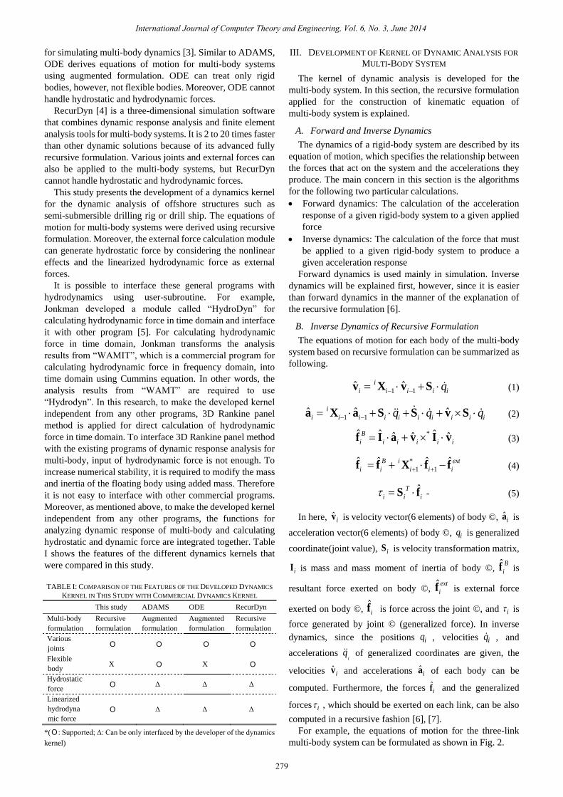
Fig. 3. Multi-body system composed of three bodies, three revolute joints,

one cylindrical joint and one closed loop.

International Journal of Computer Theory and Engineering, Vol. 6, No. 3, June 2014

280

The first test model is a multi-body system composed of

three bodies, three revolute joints, one cylindrical joint, and

one closed loop, as shown in Fig. 3.

Body 1 is attached to the base by revolute joint 1, and body

2 is connected to body 1 by revolute joint 2. Body 3 is

attached to body 2 with revolute joint 3, and moves

perpendicular to the x axis due to cylindrical joint 1.

Position Velocity Acceleration

Calculation

result from

reference

Result

calculated

using

developed

kernel 0.0

0.5

1.0

1.5

2.0

2.5

3.0

3.5

0.0 0.5 1.0

q1

q2

-4.0

-2.0

0.0

2.0

4.0

0 0.5 1

q1_dot

q2_dot

-15.0

-10.0

-5.0

0.0

5.0

10.0

15.0

0 0.5 1

q1_twodot

q2_twodot

t[sec]

[rad/s][rad/s] [rad/s2]

t[sec]t[sec]

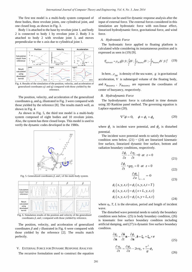
Fig. 4. Results of the simulation of the position, velocity, and acceleration of

generalized coordinates q1 and q2 compared with those yielded by the

reference.

The position, velocity, and acceleration of the generalized

coordinates q1 and q2 illustrated in Fig. 3 were compared with

those yielded by the reference [8]. The results match well, as

shown in Fig. 4

As shown in Fig. 5, the third test model is a multi-body

system composed of eight bodies and 10 revolute joints.

Also, the system has three closed loops. This model is used to

verify the dynamic codes developed in the 1980s.

Fig. 5. Generalized coordinates β, and γ of the multi-body system.

Calculation

result from

reference

Result

calculated

using

developed

kernel

0.00E+00

5.00E-02

1.00E-01

1.50E-01

2.00E-01

2.50E-01

3.00E-01

3.50E-01

4.00E-01

4.50E-01

5.00E-01

0 0.005 0.01 0.015 0.02 0.025 0.03 0.035

Gaama

-2.00E+02

-1.50E+02

-1.00E+02

-5.00E+01

0.00E+00

5.00E+01

1.00E+02

1.50E+02

2.00E+02

0 0.005 0.01 0.015 0.02 0.025 0.03 0.035

Gaama_dot

0.00E+00

2.00E+02

4.00E+02

6.00E+02

8.00E+02

1.00E+03

1.20E+03

0 0.005 0.01 0.015 0.02 0.025 0.03 0.035

Beta_dot

0.00E+00

2.00E+00

4.00E+00

6.00E+00

8.00E+00

1.00E+01

1.20E+01

1.40E+01

1.60E+01

1.80E+01

0 0.005 0.01 0.015 0.02 0.025 0.03 0.035

Beta

Fig. 6. Simulation results of the position and velocity of the generalized

coordinates β, and γ compared with those yielded by reference.

The position, velocity, and acceleration of generalized

coordinates β and γ illustrated in Fig. 6 were compared with

those yielded by the reference [2]. The results match

perfectly.

V. EXTERNAL FORCE FOR DYNAMIC RESPONSE ANALYSIS

The recursive formulation used to construct the equation

of motion can be used for dynamic response analysis after the

input of external force. The external forces considered in this

simulation are hydrostatic force with non-linear effect,

linearized hydrodynamic force, gravitational force, and wind

force.

A. Hydrostatic Force

The hydrostatic force applied to floating platform is

calculated while considering its instantaneous position and is

expressed as seen in (19) [9].

[0 ;0 ; ; ; ;0 ]e T

Hydrostatic SW Buoyancy Buoyancy

V V V

g dV y dV x dV f (19)

In here, SW

is density of the sea water, g is gravitational

acceleration, V is submerged volume of the floating body,

andBuoyancyx ,

Buoyancyy are represent the coordinates of

center of buoyancy, respectively.

B. Hydrodynamic Force

The hydrodynamic force is calculated in time domain

using 3D Rankine panel method. The governing equation is

Laplace equation (20).

2 0, I d (20)

where I is incident wave potential, and d is disturbed

potential.

The incident wave potential needs to satisfy the boundary

condition seen below. (21) ~ (24) are linearized kinematic

free surface, linearized dynamic free surface, bottom and

radiation boundary conditions, respectively.

=0 0I I at zz t

(21)

+ 0 0IIg at z

t

(22)

0I

z hz

(23)

, , , , , ,

, , , , , ,

, , , , , ,

I I

I I

I I

x y z t x y z t T

x y z t x L y z t

x y z t x y L z t

(24)

where ηI, T, L is the elevation, period and length of incident

wave.

The disturbed wave potential needs to satisfy the boundary

condition seen below. (25) is body boundary condition, (26)

is kinematic free surface boundary condition including

artificial damping, and (27) is dynamic free surface boundary

condition.

,d IT R

t

δn δ ξ ξ r

n n (25)

2

2d d

d dt z g

(26)

International Journal of Computer Theory and Engineering, Vol. 6, No. 3, June 2014

281

( ) 0ddg t dt

t

(27)

where δ is position vector of the panel of floating body

defined in inertial coordinate system, r is position vector of

the panel of floating body defined in body-fixed coordinate

system, ξT is position vector ,1 ,2 ,3( , , )P P Pq q q of center of

mass for object defined in inertia coordination, ξR is angular

vector ,4 ,5 ,6( , , )P P Pq q q defining the orientation of body-fixed

coordinate system, ηd is wave elevation of the disturbed

potential, and represents radiation coefficient.

Problems defined as above can be solved as follows.

Incident wave potential I have analytic solution (28).

sin cos sinkz

I

gAe kx ky t

(28)

where A is wave amplitude, k is wave number, is wave

direction, is wave frequency.

Then disturbed potential d is calculated using numerical

method. In this case, the Green’s second identity is used as

seen in (29), and for G the 3D Rankine Source in (30) is used

[10].

Body F

d dd d d

S S

G GG dS G dS

n n n n

(29)

1 1( , )

4G

x x

x x (30)

In here, x is position vector of 3D Rankine source, x' is

position vector of panels, Sbody is body surface, and SF is free

surface.

To increase the numerical stability of this procedure, when

we calculate acceleration of the ship at time (t+dt), ( )t dta ,

( )add tm a is considered as the additional external force

with the hydrodynamic force at time (t+1), and addm is added

to real mass of the floating body. This is the reason why it is

not very simple to apply the 3D Rankine panel method to the

commercial program for multi-body response analysis. In

here, addm is added mass and it is also calculated using 3D

Rankine panel method.

VI. SIMULATION OF LAUNCHING A SHIP USING TWO

FLOATING CRANE

Fig. 1 (b) shows a case of using 2 floating cranes for

launching a ship built on land due to the shortage of dock.

The weight of the constructed ship in this case is 3,800ton

before setting up the accommodations and other equipment.

The capacity of the floating crane used in this process is

3,000ton each. The reason for using two floating cranes is

due to the weight of ship exceeding the capability of single

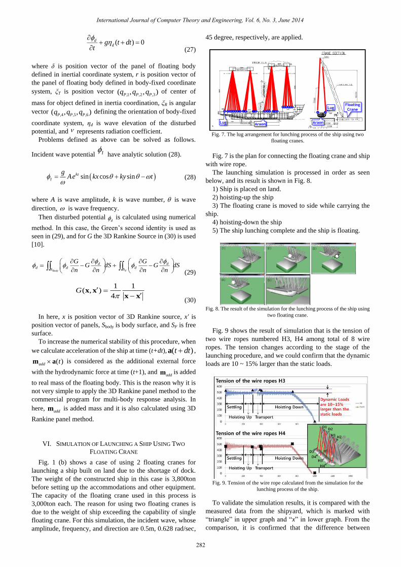
floating crane. For this simulation, the incident wave, whose

amplitude, frequency, and direction are 0.5m, 0.628 rad/sec,

45 degree, respectively, are applied.

Lug Araon Araon

LugFloating

Crane

Fig. 7. The lug arrangement for lunching process of the ship using two

floating cranes.

Fig. 7 is the plan for connecting the floating crane and ship

with wire rope.

The launching simulation is processed in order as seen

below, and its result is shown in Fig. 8.

1) Ship is placed on land.

2) hoisting-up the ship

3) The floating crane is moved to side while carrying the

ship.

4) hoisting-down the ship

5) The ship lunching complete and the ship is floating.

(1) (2)

(3) (4)

(5)

(1) (2)

(3) (4)

(5)

(1) (2)

(3) (4)

(5)

(1) (2)

(3) (4)

(5)

Fig. 8. The result of the simulation for the lunching process of the ship using

two floating crane.

Fig. 9 shows the result of simulation that is the tension of

two wire ropes numbered H3, H4 among total of 8 wire

ropes. The tension changes according to the stage of the

launching procedure, and we could confirm that the dynamic

loads are 10 ~ 15% larger than the static loads.

Fig. 9. Tension of the wire rope calculated from the simulation for the

lunching process of the ship.

To validate the simulation results, it is compared with the

measured data from the shipyard, which is marked with

“triangle” in upper graph and “x” in lower graph. From the

comparison, it is confirmed that the difference between

International Journal of Computer Theory and Engineering, Vol. 6, No. 3, June 2014

282

simulation and measured data does not exceed 10%.

This 10% difference is mainly caused by uncertainty of

synchronization between the cranes, and we are planning to

consider this uncertainty as a factor of multi-crane

simulation.

VII. SIMULATION FOR BLOCK TURNOVER USING TWO

GOLIATH CRANES

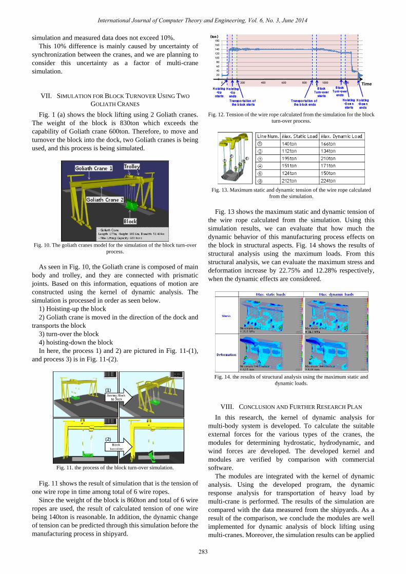
Fig. 1 (a) shows the block lifting using 2 Goliath cranes.

The weight of the block is 830ton which exceeds the

capability of Goliath crane 600ton. Therefore, to move and

turnover the block into the dock, two Goliath cranes is being

used, and this process is being simulated.

Fig. 10. The goliath cranes model for the simulation of the block turn-over

process.

As seen in Fig. 10, the Goliath crane is composed of main

body and trolley, and they are connected with prismatic

joints. Based on this information, equations of motion are

constructed using the kernel of dynamic analysis. The

simulation is processed in order as seen below.

1) Hoisting-up the block

2) Goliath crane is moved in the direction of the dock and

transports the block

3) turn-over the block

4) hoisting-down the block

In here, the process 1) and 2) are pictured in Fig. 11-(1),

and process 3) is in Fig. 11-(2).

Fig. 11. the process of the block turn-over simulation.

Fig. 11 shows the result of simulation that is the tension of

one wire rope in time among total of 6 wire ropes.

Since the weight of the block is 860ton and total of 6 wire

ropes are used, the result of calculated tension of one wire

being 140ton is reasonable. In addition, the dynamic change

of tension can be predicted through this simulation before the

manufacturing process in shipyard.

0

20

40

60

80

100

120

140

160

180

0 200 400 600 800 1000 1200 1400 1600

Tension

Time

(ton)

Transportation of the block ends

BlockTurn-over

starts

BlockTurn-over

ends

H oisting-U pstarts

H oisting-U pends

Transportation of the block starts

H oisting-D ow nstarts

H oisting-D ow nends

Fig. 12. Tension of the wire rope calculated from the simulation for the block

turn-over process.

Fig. 13. Maximum static and dynamic tension of the wire rope calculated

from the simulation.

Fig. 13 shows the maximum static and dynamic tension of

the wire rope calculated from the simulation. Using this

simulation results, we can evaluate that how much the

dynamic behavior of this manufacturing process effects on

the block in structural aspects. Fig. 14 shows the results of

structural analysis using the maximum loads. From this

structural analysis, we can evaluate the maximum stress and

deformation increase by 22.75% and 12.28% respectively,

when the dynamic effects are considered.

Fig. 14. the results of structural analysis using the maximum static and

dynamic loads.

VIII. CONCLUSION AND FURTHER RESEARCH PLAN

In this research, the kernel of dynamic analysis for

multi-body system is developed. To calculate the suitable

external forces for the various types of the cranes, the

modules for determining hydrostatic, hydrodynamic, and

wind forces are developed. The developed kernel and

modules are verified by comparison with commercial

software.

The modules are integrated with the kernel of dynamic

analysis. Using the developed program, the dynamic

response analysis for transportation of heavy load by

multi-crane is performed. The results of the simulation are

compared with the data measured from the shipyards. As a

result of the comparison, we conclude the modules are well

implemented for dynamic analysis of block lifting using

multi-cranes. Moreover, the simulation results can be applied

International Journal of Computer Theory and Engineering, Vol. 6, No. 3, June 2014

283

to the structural analysis for evaluate the dynamic effects on

the block.

In further research, this simulation program will be applied

to other various simulations in order to enhance its liability.

Moreover, other several functions, for example, the

equalizer, the module for calculating contact force between

the wire rope and body, etc., will be developed to make this

program can consider more field environment.

ACKNOWLEDGMENT

This study was partially supported by the Industrial

Strategic Technology Development Program (10035331,

Simulation-based Manufacturing Technology for Ships and

Offshore Plants) funded by the Ministry of Knowledge

Economy (MKE) of the Republic of Korea and by the Brain

Korea 21 plus program of the Marine Technology Education

and Research Center, the Research Institute of Marine

Systems Engineering, and the Engineering Research Institute

of Seoul National University.

REFERENCES

[1] N. Orlandea, M. A. Chace, and D. A. Calahan, “A sparsity-oriented

approach to the dynamic analysis and design of mechanical

systems-part 1 and 2,” Journal of Engineering for Industry,

Transactions of the ASME, vol. 99, no. 3, pp. 773-779, 1977.

[2] W. Schiehlen, Multibody Systems Handbook, Springer, pp. 361-402,

1990.

[3] R. Smith, Open dynamics Engine v0.5 User Guide, pp. 15-20, 2006.

[4] FunctionBay, Inc., RecurDyn V7R5 Release Notes, 2011.

[5] J. M. Jonkman, “Dynamics of offshore floating wind turbines - model

development and verification,” Wind Energy, 2009.

[6] R. Featherstone, Rigid body Dynamics, Springer, 2008.

[7] J. Y. S. Luh, “On-line computational scheme for mechanical

manipulators,” Journal of Dynamic Systems, Measurement, and

Control, vol. 102, pp. 69-76, 1980.

[8] E. J. Haug, Intermediate Dynamics, Prentice-hall, 1992.

[9] K. Y. Lee, J. H. Cha, and K. P. Park, "Dynamic response of a floating

crane in waves by considering the nonlinear effect of hydrostatic

force," Ship Technology Research, vol. 57, no. 1, pp. 62-71, 2010.

[10] D. C. Kring, “Time domain ship motions by a three-dimensional

rankine panel method,” MIT, Ph.D. Thesis, 1994.

Namkug Ku is a research engineer of Education and

Research Center for Creative Offshore Plant Engineers at

Seoul National University, Korea. He holds a B.S., M.S.,

and Ph.D. in naval architecture and ocean engineering

from Seoul National University. His main area of research

interests include ship and offshore plant design,

multi-body dynamics, top-side process engineering of

offshore plant, and so on.

Sol Ha is a research engineer of Engineering Research

Institute at Seoul National University, Korea. He holds a

B.S., M.S., and Ph.D. in naval architecture and ocean

engineering from Seoul National University. His main

area of research interests include ship and offshore plant

design, methodology of modeling and simulation, risk and

reliability analysis, GPU-accelerated parallel processing,

fluid analysis based on lattice Boltzmann method, and so

on.

Myung-Il Roh is a professor of naval architecture and

ocean engineering at Seoul National University, Korea.

He holds a B.S., M.S., and Ph.D. in naval architecture and

ocean engineering from Seoul National University. His

main area of teaching and research interests include ship

and offshore plant design, simulation-based design and

production, optimization, CAD, CAM, CAE, CAPP, and

so on.

International Journal of Computer Theory and Engineering, Vol. 6, No. 3, June 2014

284