Crack Inspection and simulations with Eddy Current ......Crack Inspection and simulations with Eddy Current Thermography for the Aerospace Industry Mémoire Gia Phuong Tran Maîtrise

Crack Inspection and simulations with Eddy Current Thermography for the Aerospace Industry

Mémoire

Gia Phuong Tran

Maîtrise en génie électrique Maître ès sciences (M.Sc.)

Québec, Canada

© Gia Phuong Tran, 2013

ii

iii

Résumé

La Thermographie des Courants de Foucault (Eddy Current Thermography, ECT) est

une méthode de contrôle non-destructif (CND) sans contact, et de nos jours il est utilisé

dans une large gamme d'applications. Cette méthode combine les techniques de

courants de Foucault et des techniques de thermographies de type CND afin de fournir

une méthode efficace pour la détection des fissures. Dans cette méthode, le courant de

Foucault est généré dans les échantillons métalliques. Si l'échantillon contient des

fissures, le déplacement du courant et la propagation de la température à l'intérieur des

échantillons métalliques seraient affectés par ces fissures. Les changements de la

distribution de température sont captés par une caméra infrarouge.

L'un des principaux défis de cette méthode est qu'elle nécessite beaucoup de

paramètres dans les expériences, tels que l’excitation des bobines: la valeur de la

fréquence, le nombre de tours, le matériel de fil, le rayon de la bobine ... Afin d'optimiser

les expériences, la simulation numérique est nécessaire, et le logiciel COMSOL

Multiphysics® FEM est une solution très appropriée.

Pendant le processus de simulation, une limite de détection de fissure a été proposée

pour une fissure dans un spécimen métallique donné. Les résultats de la simulation et

de la limite de détection des fissures sont également vérifiés au moyen d’expériences en

laboratoire.

L'objectif final de cette thèse est de fournir une image globale de la Thermographie des

Courants de Foucault, la limite de détection des fissures et la manière dont la simulation

ainsi que les expériences doivent être effectue afin de détecter les fissures dans les

échantillons de plaques métalliques. Ces échantillons ont été fournis par L3-MAS et

Pratt & Whitney Canada (PWC), les partenaires industriels impliqués dans ce projet quia

été financé par le Conseil de recherches en sciences naturelles et en génie du Canada

(CRSNG) et le Consortium de recherche et d'innovation en aérospatiale au Québec

(CRIAQ).

iv

v

Abstract

Eddy Current Thermography (ECT) is a non-contact, non-destructive testing (NDT)

method, and nowadays it is used in a wide range of applications. This method combines

eddy current and thermographic NDT techniques in order to provide an efficient method

for crack detection. In this method, the eddy current is generated into metallic

specimens. If the specimen contains cracks, the current flow and temperature

propagation inside the metallic specimens would be affected by these cracks. The

changes of temperature distribution are captured by an infrared camera.

One of the main challenges in this method is that it requires many parameters in the

experiments, such as coil excitations: the frequency value, number of turns, material of

wire, radius of the coil...In order to optimize the experiments, numerical simulation is

necessary, and COMSOL Multiphysics® FEM software is a very suitable solution.

During the simulation process, a crack detection limit for a crack in a given metallic

specimen has been proposed. The simulation results and crack detection limit are also

verified using experiments in the laboratory.

The final goal of this thesis is to provide the overall picture of the Eddy Current

Thermography, crack detection limit and the manner in which to simulate as well as

perform the experiments in order to detect cracks on the metallic plate specimens which

were provided by L3-MAS and Pratt & Whitney Canada (P.W.C), the industrial partners

involved in this project which was sponsored by the Natural Sciences and Engineering

Research Council of Canada (NSERC) and The Consortium for Research and

Innovation in Aerospace in Québec (CRIAQ).

vi

vii

Acknowledgment

First of all, I would like to express my deepest gratitude to my supervisor, Professor

Xavier Maldague for his invaluable support during my studies at Université Laval. It is

truly an honor for me to be one of his students. He gave me many excellent lessons in

order to help me to build my knowledge in Electrical Engineering area, and he also

encourages me doing many research activities. My master thesis would not have been

possible without his amazing support.

I would like to thank my co-supervisor, Professor Lionel Birglen at Polytechnique

Montréal for his support and advices during my research project. I also wish to thank all

of members in the research project CRIAQ-MANU 418 for their discussions in monthly

meeting, in particular, Professor Martin Viens at École de Technologie Supérieure. He

spent so much effort to give me many advices for my research results in the monthly

meetings.

Special thanks to Marc Grenier, Denis Ouellet of the Computer Vision and Systems

Laboratory. They helped me to understand the basic steps in establishing the

experiments.

I also would like to thank the Computer and Electrical Engineering Department,

Université Laval, and the Canada Research Chair in multipolar infrared vision (MIVIM)

for the excellent resources they provided me with a very powerful computer, electrical

equipment and devices during my studies and research.

I acknowledge and greatly appreciate the financial support of The Consortium for

Research and Innovation in Aerospace in Québec (CRIAQ), and also the Natural

Sciences and Engineering Research Council of Canada (NSERC) for the project CRIAQ

MANU-418.

Finally, I would like to thank all of my teammates at the Canada Research Chair in

Multipolar Infrared Vision (MIVIM), Vietnamese students and international students at

Université Laval, who made my 2 years in Quebec City to be one of the best moments in

my life.

viii

ix

Table of Contents Résumé .......................................................................................................................... iii

Abstract ........................................................................................................................... v

Acknowledgment ........................................................................................................... vii

Chapter 1 Project description .......................................................................................... 2

1.1 Description of the sub-project ............................................................................ 2

1.2 Scientific and technical issues ........................................................................... 3

Chapter 2 Infrared Thermography for Nondestructive Testing ......................................... 4

2.1 Passive Thermography ..................................................................................... 4

2.2 Active Thermography ........................................................................................ 4

2.2.1 Lock-in thermography and Optical excitation with LT ..................................... 5

2.2.2 Pulse thermography (PT) and Optical excitation with PT ............................... 7

2.2.3 Experimental setup for optical thermography ................................................. 8

2.2.4 Step heating (SH) .......................................................................................... 9

2.2.5 Ultrasound thermography (UT) ...................................................................... 9

2.3 Advantage and difficulties of IR thermography .................................................. 9

Chapter 3 Eddy Current Thermography......................................................................... 11

3.1 Fundamental concepts ......................................................................................... 11

3.1.1 Basic electrical theory.................................................................................... 11

3.1.2 Resistance and Joule heating........................................................................ 12

3.1.3 Electromagnetic field ..................................................................................... 12

3.1.4 Hysteresis ..................................................................................................... 14

3.1.5 Skin depth ..................................................................................................... 14

3.1.5 Heat conduction ............................................................................................ 16

3.2 Eddy Current Thermography system ................................................................... 16

3.3 Advantages and limitations .................................................................................. 17

3.4 Applications ......................................................................................................... 17

Chapter 4 Simulations ................................................................................................... 18

4.1 COMSOL Multiphysic software ............................................................................ 18

4.1.1 Introduction ................................................................................................... 18

4.1.2 Working environment..................................................................................... 18

4.1.3 The Model Builder and the Model Tree .......................................................... 21

4.1.3 Model library .................................................................................................. 22

x

4.1.4 Workflow and Sequence of Operations ......................................................... 23

4.2 Mathematical models of Eddy Current Thermography ......................................... 24

4.3 Simulation results ................................................................................................ 25

4.3.1 2-D simulation results .................................................................................... 26

4.3.2 3-D simulation result ...................................................................................... 27

Chapter 5 Equipment and experimentation parameters ................................................. 30

5.1 Experimental setup .............................................................................................. 30

5.2 Infrared Camera ................................................................................................... 31

5.3 Amplifier and waveform generator ....................................................................... 33

5.4Coil ....................................................................................................................... 34

5.5 Robotic arm- the scanning table .......................................................................... 34

5.6 Specimens ........................................................................................................... 35

Chapter 6 Results ......................................................................................................... 38

6.1 Crack detection limit............................................................................................. 38

6.2 Experimental results ............................................................................................ 40

6.3 Discussion ........................................................................................................... 42

Chapter 7 Conclusion .................................................................................................... 44

Bibliography .................................................................................................................. 45

Appendix 1: User guide for modeling EC Thermography in COMSOL Multiphysics 4.3a48

Appendix 2: User guide for the X-Y table ....................................................................... 52

Appendix 3: User guide to perform ECT experiments .................................................... 55

xi

List of Tables

Table 4. 1: The thermal and coil’s excitation parameters for simulations .............................. 25

Table 5.1: Crack information ................................................................................................................ 36

Table 6.1 : Statistic information about cracks ................................................................................. 42

List of Figures Figure 2. 1: Experimental setup for active thermography [16]. ................................................... 5

Figure 2. 2 : Schematic configuration of lock-in thermography [6]. ............................................ 6

Figure 2. 3 : Schematic configuration of pulsed thermography [6]. ........................................... 7

Figure 2. 4 : Schematic setup of optical excitation thermography (Reflection mode). ......... 9

Figure 3. 1 : Resistive elements in circuit. ....................................................................................... 12

Figure 3. 2 : Induction coil with electromagnetic field [24]. ......................................................... 13

Figure 3. 3 : Reference depth for several materials [22] ............................................................. 15

Figure 3. 4 : Excitation frequency and magnetic properties [27]. ............................................. 15

Figure 3. 5 : A schematic setup of Eddy Current Thermography for NDT [16]. ................... 16

Figure 4. 1 : COMSOL integrated development environment. .................................................. 19

Figure 4. 2 : Settings window............................................................................................................... 20

Figure 4. 3 : Preference window. ........................................................................................................ 20

Figure 4. 4 : Global Definitions and Results nodes....................................................................... 21

Figure 4. 5 : Parameters........................................................................................................................ 21

Figure 4. 6 : Result node. ...................................................................................................................... 22

Figure 4. 7 : Model and Study nodes. ............................................................................................... 22

Figure 4. 8 : Model Library examples. ............................................................................................... 23

Figure 4. 9 : Workflow and sequence of operations. .................................................................... 23

Figure 4. 10 : 2-D simulation of Eddy Current Thermography. ................................................. 26

Figure 4. 11 : Induction heating simulation in 2-D. ........................................................................ 27

Figure 4. 12 : 3-D simulation of Eddy Current Thermography. ................................................. 28

Figure 4. 13 : Geometry of Induction heating simulations in 3-D. ............................................ 28

Figure 5. 1 : Experiment setup ............................................................................................................ 30

Figure 5. 2 : Experimental diagram. ................................................................................................... 31

Figure 5. 3: Infrared Camera in ECT experiment. ......................................................................... 31

Figure 5. 4: IR camera software. ........................................................................................................ 32

Figure 5. 5: Amplifier. ............................................................................................................................. 33

Figure 5. 6: Generator. ........................................................................................................................... 34

xii

Figure 5. 7: Coil and specimen. .......................................................................................................... 34

Figure 5. 8: X-Y table. ............................................................................................................................ 35

Figure 5. 9: X-Y table software control. ............................................................................................ 35

Figure 5. 10: A steel-based sample from the laboratory. ........................................................... 36

Figure 5. 11: A nickel-based specimen with a visible calibrated crack. .................................. 36

Figure 6. 1: The approach for crack detection limit....................................................................... 39

Figure 6. 2: The 3-D curve of crack detection limit (from simulated data). ............................ 40

Figure 6. 3: Detected cracks on the sample – the big one. ........................................................ 40

Figure 6. 4: Detected cracks on specimen #01(a) and #51(b). ................................................. 41

Figure 6. 5: Detected cracks on specimen # 57(a) and # 32(b). .............................................. 41

Figure 6. 6 : Crack extraction steps ................................................................................................... 42

Figure 6. 7 : Detected and non-detected cracks ............................................................................ 43

List of Equations

Equation (2. 1): Temperature at the time and depth z in LT. ....................................................... 6

Equation (2. 2): Diffusion length. .......................................................................................................... 6

Equation (2. 3): Temperature at the time and depth z in PT........................................................ 8

Equation (2. 4): Temperature at the surface in PT. ........................................................................ 8

Equation (3.1): Voltages ........................................................................................................................ 11

Equation (3. 2): Voltages in a circuit with two resistors ............................................................... 11

Equation (3. 3): Losses power ............................................................................................................. 12

Equation (3. 4): Joule heating .............................................................................................................. 12

Equation (3. 5): Skin depth ................................................................................................................... 14

Equation (4. 1): The governing equation .......................................................................................... 24

Equation (4. 2): The generated resistive heat ................................................................................ 24

Equation (4. 3): The temperature dependent electrical conductivity ....................................... 24

xiii

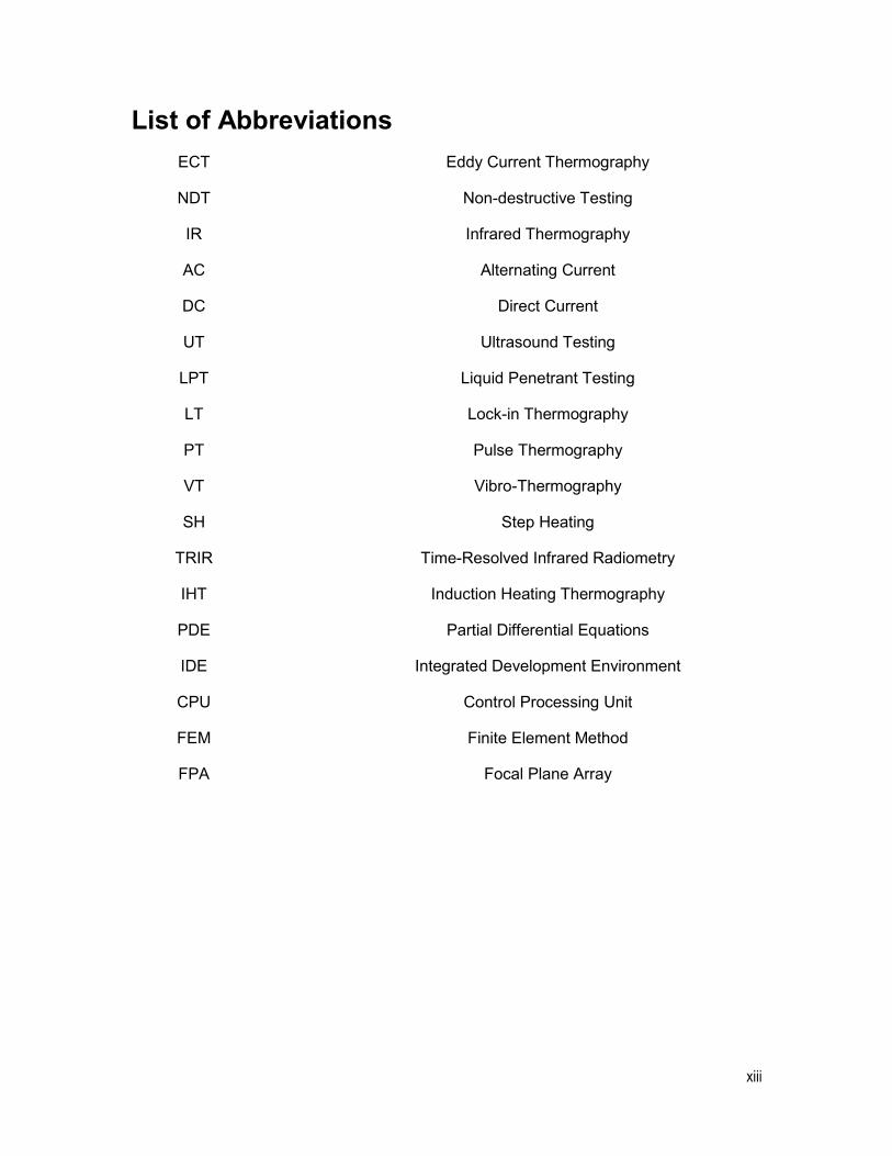
List of Abbreviations

ECT Eddy Current Thermography

NDT Non-destructive Testing

IR Infrared Thermography

AC Alternating Current

DC Direct Current

UT Ultrasound Testing

LPT Liquid Penetrant Testing

LT Lock-in Thermography

PT Pulse Thermography

VT Vibro-Thermography

SH Step Heating

TRIR Time-Resolved Infrared Radiometry

IHT Induction Heating Thermography

PDE Partial Differential Equations

IDE Integrated Development Environment

CPU Control Processing Unit

FEM Finite Element Method

FPA Focal Plane Array

xiv

1

Introduction

Over the last few decades, non-destructive testing (NDT) has been using in many

industrial branches, in order to indicate the presence of material discontinuities, such as

defects on the surface of material. There are several common methods of NDT, for

example: Ultrasound Testing (UT), Liquid Penetrant Testing (LPT), Infrared

Thermography (IR) Testing, and so on. In crack inspection, Eddy Current Thermography

is the field of IR testing; itis being widely used as a valuable testing method in many

industries, particularly in the aerospace industry in which the machine components often

have complex structures.

The Computer and Electrical Engineering Department, Université Laval, and the Canada

Research Chair in multipolar infrared vision (MIVIM) provide excellent resources for

Eddy Current Thermography experiments and simulations, including the electrical

devices, a collection of software and powerful computer which are necessary for

processing data. In this project, the metallic plate specimens are provided by the

industrial partners: L-3 and PWC.

The research work and results are organized in the following chapters.

In chapter 1 of this thesis, the project description is exposed along with the problems

which needed to be solved. The information related to the Infrared Thermography part

from original documentation of the project CRIAQ-MANU 418 is also included.

Chapter 2 provides the basic information about Infrared Thermography for NDT, the

advantages and the applications of IR techniques in industry. Chapter 3 describes

general information about Eddy Current Thermography. The theory of ECT and

fundamental concepts are reviewed in this chapter.

The detailed information about simulations is provided in chapter 4. This chapter

provides the introduction to COMSOL software, and the chosen module: Induction

Heating is described in detail. The individual results we obtained during this process are

provided as well.

Apparatus and experiments are presented in chapter 5. Detailed information about the

needed devices required by experiment is described in this chapter.

Chapter 6 focuses on the research results, including simulation and experiment results.

The 3-D curve is proposed in this chapter, and experimental results are matched with

that 3-D curve as well.

Chapter 7 gives some remarks, conclusions and future work of this research. Appendix 1

presents the basic steps to simulate ECT in COMSOL software. Appendix 3 gives

detailed guide for performing experiments in the laboratory.

2

Chapter 1 Project description

This research project is part of the project CRIAQ MANU-418: “Automated Non

Destructive Testing for the Aerospace Industry”. The information of this chapter is mainly

extracted from project description of the project CRIAQ MANU-418 [1].

The main objective of the project CRIAQ MANU-418 is to automate (NDT) systems used

in the aerospace industry in order to establish inspection procedures as well as to

enhance systems sensitivity, reliability and repeatability. At the moment, these tasks are

performed by human inspectors whose diversified experience may lead to variation in

results interpretation. A standard robotic system would be used to handle the probe

associated with each NDT techniques. Based on data provided by a 3D laser system

and using CAD files if available, an initial scanning path will be generated. In case CAD

files are not available or not reliable (particularly for in-service or modified components),

an initial or largest envelope volume will be used instead. Data fusion algorithms will be

used to build a defect database map of the inspected surface and to refine the scanning

path in subsequent passes.

Finally, an intelligent expert system will provide the user with a decision on whether a

defect is present or not, based on the interpretation of the signals from the probes. The

final result of this project will be a functional small-scale robotic NDT inspection workcell

that will serve as a benchmark for comparison with human inspectors. In addition, it is

proposed to evaluate novel NDT schemes such as Eddy Current-induced Infrared

Thermography. This novel scheme allows collecting thermal infrared signatures from

induced Eddy currents. Hence, the additional information becomes available from

subsurface defects. It is planned to fuse this information with data from the others

sensors as well: Fluorescent Penetrant Inspection and Eddy Current Testing.

1.1 Description of the sub-project

The previous paragraph provides introduction to the project CRIAQ MANU-418. In this

part, we will describe its sub-project in Infrared Thermography.

As previously mentioned, a standard robotic system will be used to handle the Eddy

Current probe to carry the inspection. And a thermal camera (infrared camera) is added

to record the thermal signature that appears on the surface of the components following

the Eddy current excitation. Finally, the system is fully autonomous and provides a final

diagnosis to the human inspectors with a minimum intervention from them.

This approach may bring many benefits to the industry since the position of component

referring to the robotic arm is totally relaxed, a conventional Eddy current inspection

would be carried out as traditionally done. Moreover, thermographic data is acquired and

thus, it is possible to bring additional information to increase the combination of

information coming from the different sensing techniques rather than from one technique

only.

3

At the beginning, the 3D camera enables acquiring the part geometry prior to inspection.

After the part geometry is calibrated, the robotic arm is enabled in the second step, in

order to perform the inspection while maintaining the end effector always perpendicular

to the inspected surface and also at the same fixed distance. Moreover, the robot covers

the surface to inspect at a constant speed (in a raster fashion). The 3D camera is shut

off and only the Eddy Current and Infrared Camera are operated. The Eddy Current and

thermal data are acquired at this stage. The defects will be detected automatically by

using software.

For automatic detection, it is proposed to analyze independently both channels (Eddy

current and IR) and combine the processed data not at the pixel level but rather at a

higher level of decision.

1.2 Scientific and technical issues

In order to obtain good results with non-destructive testing system based on Infrared

Thermography technique, we have to deal with a number of challenges, including the

scientific and technical issues as described below.

The total inspection time should be minimized by optimizing the experiment process.

Therefore, it is necessary to use numerical simulations, and COMSOL Multiphysics®

FEM software is the right choice for Infrared Thermography simulation. The detailed

information about simulations and COMSOL would be described in chapter 4.

In addition, during the experiments there will be a number of detected cracks and non-

detected cracks. Based on the capability of given infrastructure and information about

specimen material, we should know the limit of crack detection for cracks in the given

metallic specimens. This task would also be extremely challenging.

4

Chapter 2 Infrared Thermography for Nondestructive

Testing

Infrared Thermography (IR) is an efficient non-destructive testing method. It is being

widely used in different fields. It is an inspection method for examination of a part of a

specimen, a material, or a complex machine without destroying its usefulness [2].

The basic principle of Infrared Thermography is to thermally excite an object by heating

(or cooling) it while using infrared camera to monitor the changes of the object’s surface

temperature. Since the temperature flow will be affected by the subsurface

discontinuities, and these discontinuities also called defects which could be detected [3].

The knowledge of heat transfer would be presented in the next chapter, when we

describe the major NDT method of this thesis: Eddy Current Thermography.

Infrared Thermography can be used in either a passive or an active manner, which are

called passive thermography and active thermography, respectively. In the following

sections, we will describe the basic information about each approach.

2.1 Passive Thermography

Passive thermography relies on natural heat diffusion on the surface of either a

component or a structure, and it is normally employedin production, predictive

maintenance, road traffic monitoring, agriculture and biology, medicine, fire forest

detection, building thermal efficiency survey, and in NDT.

In passive thermography, the surface temperature for evaluation is measured directly.

The different temperature with respect to the surrounding is the most important

parameter, often referred to as the ’delta-T’ or the “hot spot.” A delta-T of 1 to 2 Kelvin is

generally found suspicious while a 4K value is a strong evidence of abnormal behavior

[5]. The features of interest in a given region are naturally at a higher or lower

temperature with respect to the surrounding.

2.2 Active Thermography

In contrast to passive thermography, active thermography measures the surface

temperature for evaluation after applying a thermal excitation source. There is an

external energy source required in this approach in order to produce a thermal contrast

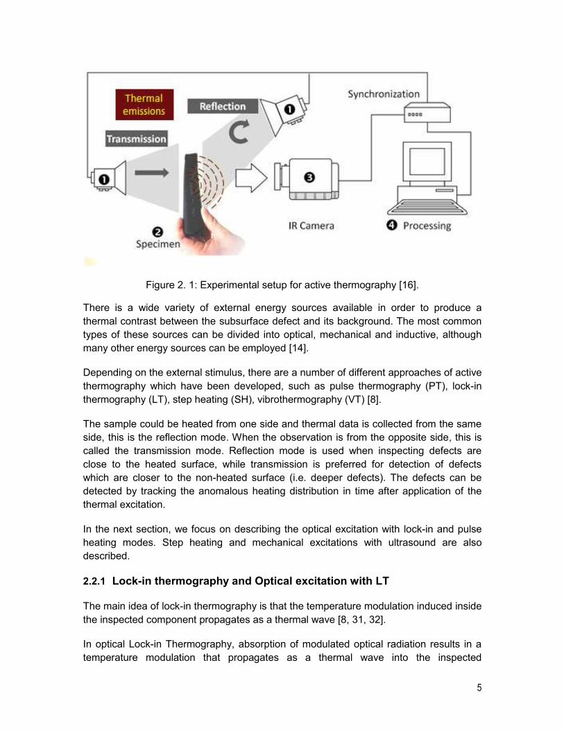
between the feature of interest in a given region and its background as shown in Figure

2.1 below:

5

Figure 2. 1: Experimental setup for active thermography [16].

There is a wide variety of external energy sources available in order to produce a

thermal contrast between the subsurface defect and its background. The most common

types of these sources can be divided into optical, mechanical and inductive, although

many other energy sources can be employed [14].

Depending on the external stimulus, there are a number of different approaches of active

thermography which have been developed, such as pulse thermography (PT), lock-in

thermography (LT), step heating (SH), vibrothermography (VT) [8].

The sample could be heated from one side and thermal data is collected from the same

side, this is the reflection mode. When the observation is from the opposite side, this is

called the transmission mode. Reflection mode is used when inspecting defects are

close to the heated surface, while transmission is preferred for detection of defects

which are closer to the non-heated surface (i.e. deeper defects). The defects can be

detected by tracking the anomalous heating distribution in time after application of the

thermal excitation.

In the next section, we focus on describing the optical excitation with lock-in and pulse

heating modes. Step heating and mechanical excitations with ultrasound are also

described.

2.2.1 Lock-in thermography and Optical excitation with LT

The main idea of lock-in thermography is that the temperature modulation induced inside

the inspected component propagates as a thermal wave [8, 31, 32].

In optical Lock-in Thermography, absorption of modulated optical radiation results in a

temperature modulation that propagates as a thermal wave into the inspected

6

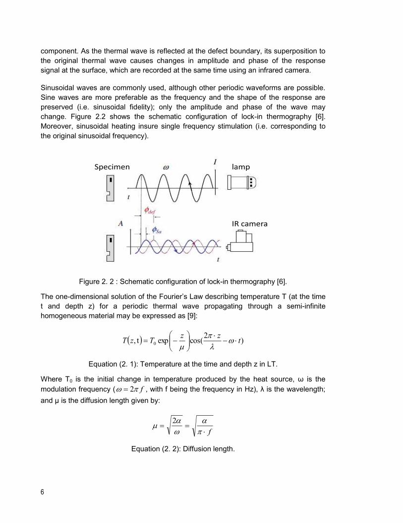
component. As the thermal wave is reflected at the defect boundary, its superposition to

the original thermal wave causes changes in amplitude and phase of the response

signal at the surface, which are recorded at the same time using an infrared camera.

Sinusoidal waves are commonly used, although other periodic waveforms are possible.

Sine waves are more preferable as the frequency and the shape of the response are

preserved (i.e. sinusoidal fidelity); only the amplitude and phase of the wave may

change. Figure 2.2 shows the schematic configuration of lock-in thermography [6].

Moreover, sinusoidal heating insure single frequency stimulation (i.e. corresponding to

the original sinusoidal frequency).

Figure 2. 2 : Schematic configuration of lock-in thermography [6].

The one-dimensional solution of the Fourier’s Law describing temperature T (at the time

t and depth z) for a periodic thermal wave propagating through a semi-infinite

homogeneous material may be expressed as [9]:

)2

cos(expt, 0 tzz

TzT

Equation (2. 1): Temperature at the time and depth z in LT.

Where T0 is the initial change in temperature produced by the heat source, ω is the

modulation frequency ( f 2 , with f being the frequency in Hz), λ is the wavelength;

and μ is the diffusion length given by:

f

2

Equation (2. 2): Diffusion length.

lamp

IR camera

Specimen

7

Where c / is the diffusivity of material, with being the thermal conductivity, ρ the

density, c the specific heat; and f 2 is the frequency modulation.

The thermal diffusion length increases with deducing modulation frequency ω as

shown in equation 2.2. The probing depth z, for amplitude images is given by the

diffusion length, z~μ [10]. For the phase, reported values range from 1.5 to more than

2 [11]. To detect defects on different depths we have to use a range of frequencies

roughly corresponding to μ. Deep defects require very low frequency, which of course

lengthens the inspection time.

2.2.2 Pulse thermography (PT) and Optical excitation with PT

Pulse thermography (PT) is one of the most common thermal stimulation methods used

in active thermography for nondestructive testing. One reason for this is the quickness of

the inspection, in which a short thermal stimulation pulse lasting from a few milliseconds

for high conductivity materials, such as metal, to a few seconds for low conductivity

specimen, such as plastics, is used [5, 12,13].

In optical Pulse Thermography, the surface of specimen is submitted to a short heat

pulse using a high power optical source. The duration of the pulse may vary from a few

ms (~2-15 ms using flashes) to several seconds (using lamps). Absorption of short time

pulse energy elevates the specimen surface temperature. As time elapses and the

heating pulse vanishes, the surface temperature will decrease uniformly for a piece

without internal flaws.

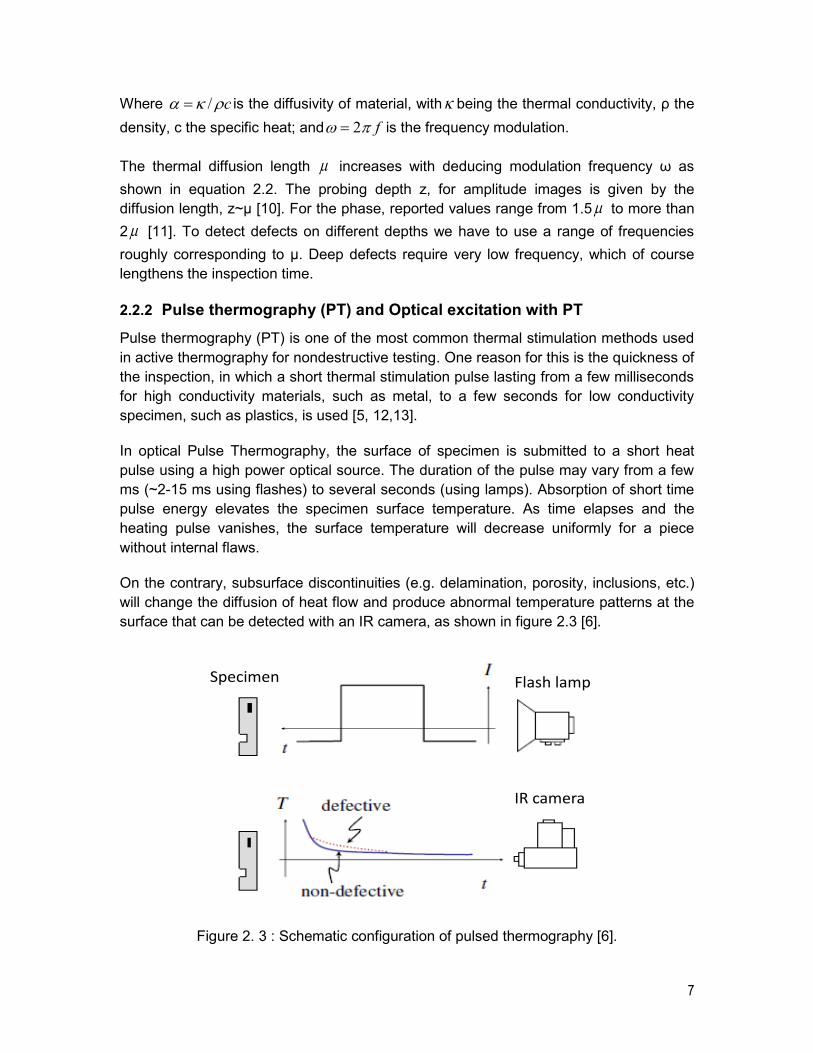
On the contrary, subsurface discontinuities (e.g. delamination, porosity, inclusions, etc.)

will change the diffusion of heat flow and produce abnormal temperature patterns at the

surface that can be detected with an IR camera, as shown in figure 2.3 [6].

Figure 2. 3 : Schematic configuration of pulsed thermography [6].

Flash lamp

IR camera

Specimen

8

The one-dimensional solution of the Fourier’s Law for a Dirac delta pulse propagating

through a semi-infinite homogeneous material is given by [33]:

t

z

tc

QTtzT

4exp,

2

0

Equation (2. 3): Temperature at the time and depth z in PT.

Where Q is the energy absorbed by the surface, T0 is the initial temperature.

Considering the surface time evolution, Eq. (2.3) can be rewritten as (z=0):

te

QTtT

0,0

Equation (2. 4): Temperature at the surface in PT.

Where ce is the diffusivity, which is a thermal property that measures the

material ability to exchange heat with its surrounding.As seen from the previous

equation, temperature decreases approximately as t1/2 (at least at early times).

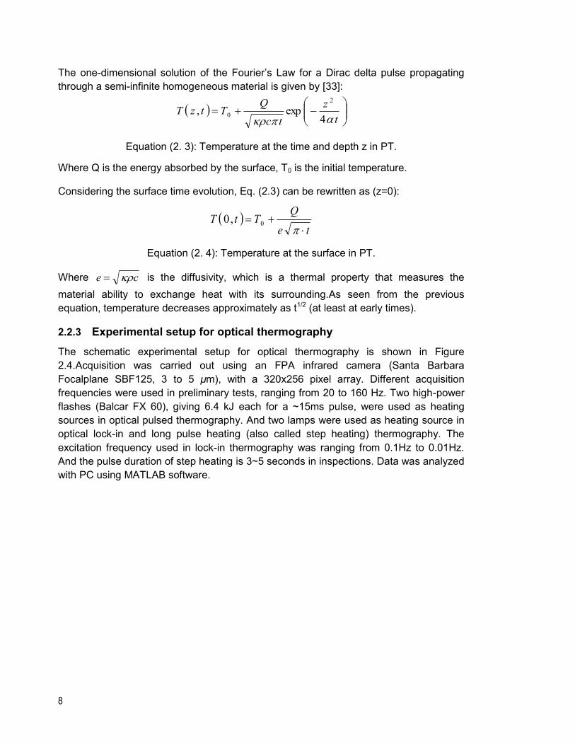
2.2.3 Experimental setup for optical thermography

The schematic experimental setup for optical thermography is shown in Figure

2.4.Acquisition was carried out using an FPA infrared camera (Santa Barbara

Focalplane SBF125, 3 to 5 μm), with a 320x256 pixel array. Different acquisition

frequencies were used in preliminary tests, ranging from 20 to 160 Hz. Two high-power

flashes (Balcar FX 60), giving 6.4 kJ each for a ~15ms pulse, were used as heating

sources in optical pulsed thermography. And two lamps were used as heating source in

optical lock-in and long pulse heating (also called step heating) thermography. The

excitation frequency used in lock-in thermography was ranging from 0.1Hz to 0.01Hz.

And the pulse duration of step heating is 3~5 seconds in inspections. Data was analyzed

with PC using MATLAB software.

9

Figure 2. 4 : Schematic setup of optical excitation thermography (Reflection mode).

2.2.4 Step heating (SH)

In contrary to Pulse Thermography scheme for which the temperature decays is of

interest (after the heat pulse), here the increase of surface temperature is monitored

during the application of a step heating (SH) pulse (long pulse). The sample is

continuously heated at low power. Variations of surface temperature with time are

related to specimen features as in pulse thermography.

This technique of stepped heating is sometimes referred to as time-resolved infrared

radiometry (TRIR) [8]. The time resolved means that the temperature is monitored as it

evolves during and after the heating process. TRIR finds applications such as for coating

thickness evaluation (including multi-layered coatings, ceramics), integrity of the coating

– substrate bond determination evaluation of composite structures.

2.2.5 Ultrasound thermography (UT)

Ultrasound thermography (UT) is an active thermography method, and its external

energy source is a mechanical excitation. This method was invented in the end of 70’s

and has been widely used in 90’s. The basic idea of this method is to induce mechanical

waves of high frequencies (usually 15~25 kHz or 40 kHz) into the specimen in order to

observe the changes of surface temperature by using an infrared camera.

This method was successfully applied to detect cracks in metals, delaminations in

composite materials and other defects both on the surface and subsurface. It is

especially used in aerospace and automotive industry.

2.3 Advantage and difficulties of IR thermography

The main advantage of Infrared Thermography in comparison to many other NDT

methods is that it makes possible to inspect large areas within a short time and in a safe

Lamp

Lamp

IR camera

PC

Specimen

10

manner without the need to have access to both sides of the component [7]. Moreover,

this method has the capacity to provide real time images of any defects which may be

present in the inspection area.

For example, with Infrared Thermography we can identify overheating of electrical

connections and other machine components. Moreover, scheduling repair is made

during planned downtime. This work helps to increase reliability and productivity for the

entire operation of products.

Beside the main advantages listed above, IR thermography has more several strengths

which make it more useful in some applications where other NDT techniques don’t

perform well enough [5, 8, 12, 13, 35]:

fast and accurate inspection rate;

non-contact approach;

wide range of applications;

results are relatively to interpret since these results are obtained in image format

and those could be processed by software in order to extract more information;

unique inspection tool for several inspection parts.

However, in addition to the advantages listed above, there are several difficulties of IR

thermography as pointed below [5, 8, 12, 13]:

cost may be a factor for using IR thermography, since the thermo-imaging

equipment, data processing and modeling software are expensive;

effect of thermal loses;

difficulty in obtaining a uniform thermal stimulation over a large surface;

IR thermography enables only to inspect a limited thickness of material under the

probed surface;

emissivity problems.

11

Chapter 3 Eddy Current Thermography

As mentioned in chapter 2, one interesting type of external source in active

thermography is inductive excitation which can be employed internally to electro-

conductive materials [14].It generates eddy currents at a specific depth which is called

penetration depth, or skin-depth. The induced current’s skin depth is determined by the

frequency of the excitation. Normally, the range of values of frequencies used in Eddy

Current Thermography (ECT) may vary from 20-200 kHz. The temperature distribution is

changed if cracks are present in the specimen, since these cracks affect the current

flow. And this change can be detected on the surface by an infrared camera. In other

words, ECT combines eddy currents and a thermographic NDT technique in order to

provide an efficient method for defect detection, such as cracks [4].

Eddy Current Thermography or Induction Heating Thermography (IHT) is the latest

development in the field of active thermography, it also received special attention in

recent years from researchers around the world [17, 18, 19,20].

In this chapter, the theory and fundamental concepts of ECT are briefly presented. The

advantages and limitations of ECT and its applications are also described.

3.1 Fundamental concepts

ECT or Induction Heating occurs due to electromagnetic force fields producing an

electrical current in a part of specimen. The part is heated because of the resistance to

the flow of this electrical current.

3.1.1 Basic electrical theory

When a voltage is applied to a circuit containing only resistive elements, current flows

according to Ohm’s Law:

I = V/R or V = I.R Equation (3.1): Voltages

If a circuit consists of more than one element, the overall voltages, resistance and

capacitance can be calculated by simple algebra, for example, with two resistors in

series, as show in Figure 3.1, current (I) must be the same for both resistors:

V1 =I.R1, V2=I.R2,

Vtotal = V1+V2 = I.R1+ I.R2 = I (R1+R2) = I.Rtotal

Equation (3. 2): Voltages in a circuit with two resistors

So Rtotal = R1+ R2.

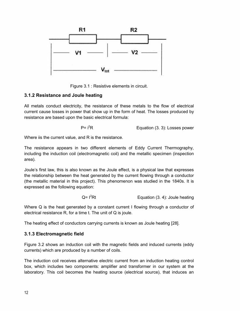
12

Figure 3.1 : Resistive elements in circuit.

3.1.2 Resistance and Joule heating

All metals conduct electricity, the resistance of these metals to the flow of electrical

current cause losses in power that show up in the form of heat. The losses produced by

resistance are based upon the basic electrical formula:

P= i2R Equation (3. 3): Losses power

Where iis the current value, and R is the resistance.

The resistance appears in two different elements of Eddy Current Thermography,

including the induction coil (electromagnetic coil) and the metallic specimen (inspection

area).

Joule’s first law, this is also known as the Joule effect, is a physical law that expresses

the relationship between the heat generated by the current flowing through a conductor

(the metallic material in this project). This phenomenon was studied in the 1840s. It is

expressed as the following equation:

Q= I2Rt Equation (3. 4): Joule heating

Where Q is the heat generated by a constant current I flowing through a conductor of

electrical resistance R, for a time t. The unit of Q is joule.

The heating effect of conductors carrying currents is known as Joule heating [28].

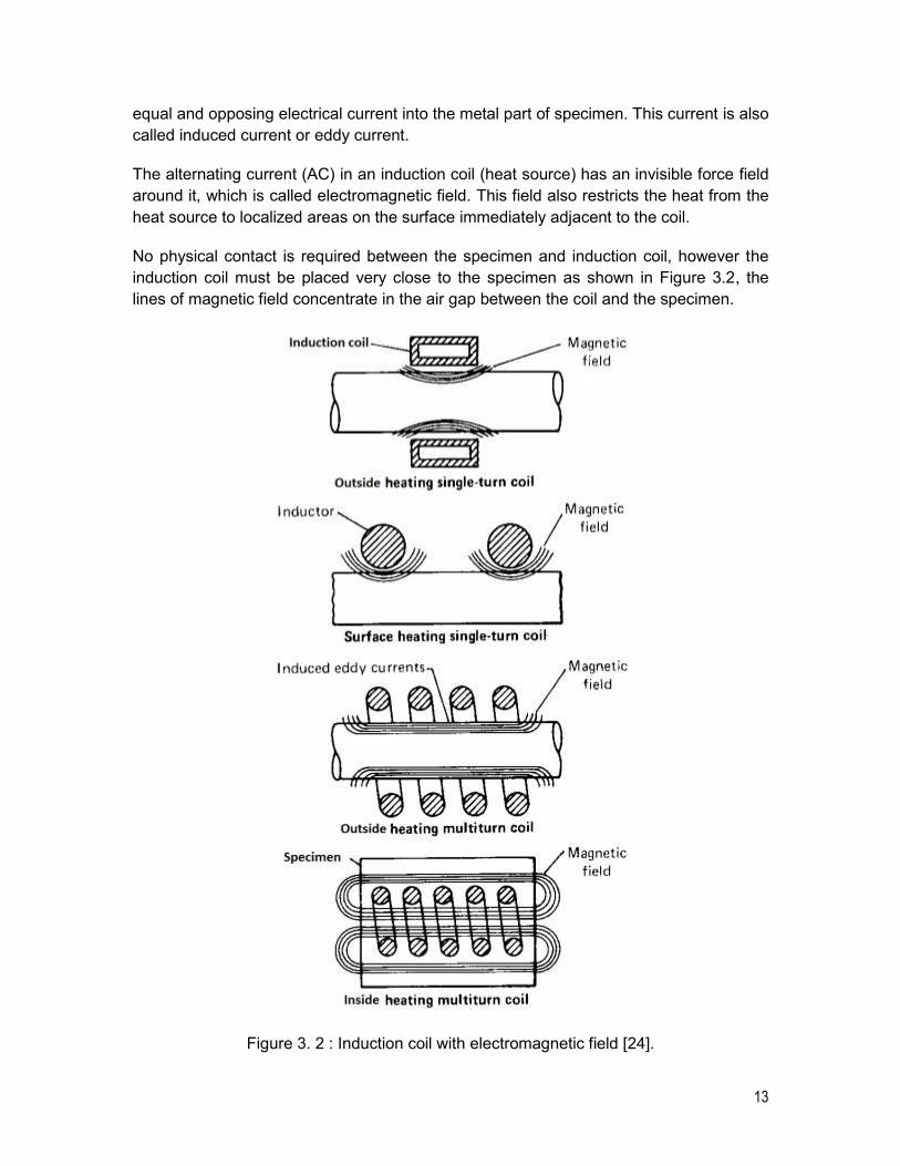
3.1.3 Electromagnetic field

Figure 3.2 shows an induction coil with the magnetic fields and induced currents (eddy

currents) which are produced by a number of coils.

The induction coil receives alternative electric current from an induction heating control

box, which includes two components: amplifier and transformer in our system at the

laboratory. This coil becomes the heating source (electrical source), that induces an

13

equal and opposing electrical current into the metal part of specimen. This current is also

called induced current or eddy current.

The alternating current (AC) in an induction coil (heat source) has an invisible force field

around it, which is called electromagnetic field. This field also restricts the heat from the

heat source to localized areas on the surface immediately adjacent to the coil.

No physical contact is required between the specimen and induction coil, however the

induction coil must be placed very close to the specimen as shown in Figure 3.2, the

lines of magnetic field concentrate in the air gap between the coil and the specimen.

Figure 3. 2 : Induction coil with electromagnetic field [24].

14

The rate of heating of specimen is dependent on the frequency and the intensity of the

induced current, the magnetic permeability of the material and the resistance of the

material to the flow of current [23].

3.1.4 Hysteresis

Hysteresis losses appear in magnetic materials, such as nickel, steel and some other

kinds of metals. For example, with the specimens made from carbon steels, when

magnetic parts of the specimens are being heated, by induction from room temperature,

the alternating magnetic flux field causes the magnetic dipoles of the material to oscillate

as the magnetic poles change their polar orientation every cycle. This oscillation is called

hysteresis [23]. Moreover, when the dipoles oscillate, the friction produced by this

oscillation will generate a minor amount of heat.

3.1.5 Skin depth

In order to make Eddy Current Thermography with Induction Heating an efficient and

practical process, certain relationships of the frequency of the electromagnetic field that

produce the eddy currents and the properties of the specimen under inspection must be

satisfied. These relationships are often referred to as “skin-depth”, or reference depth

(depth of penetration).

They are described in the following equation [4, 27]:

Skin depth √

Equation (3. 5): Skin depth

With: angular frequency ,

permeability µ = µ0µr,

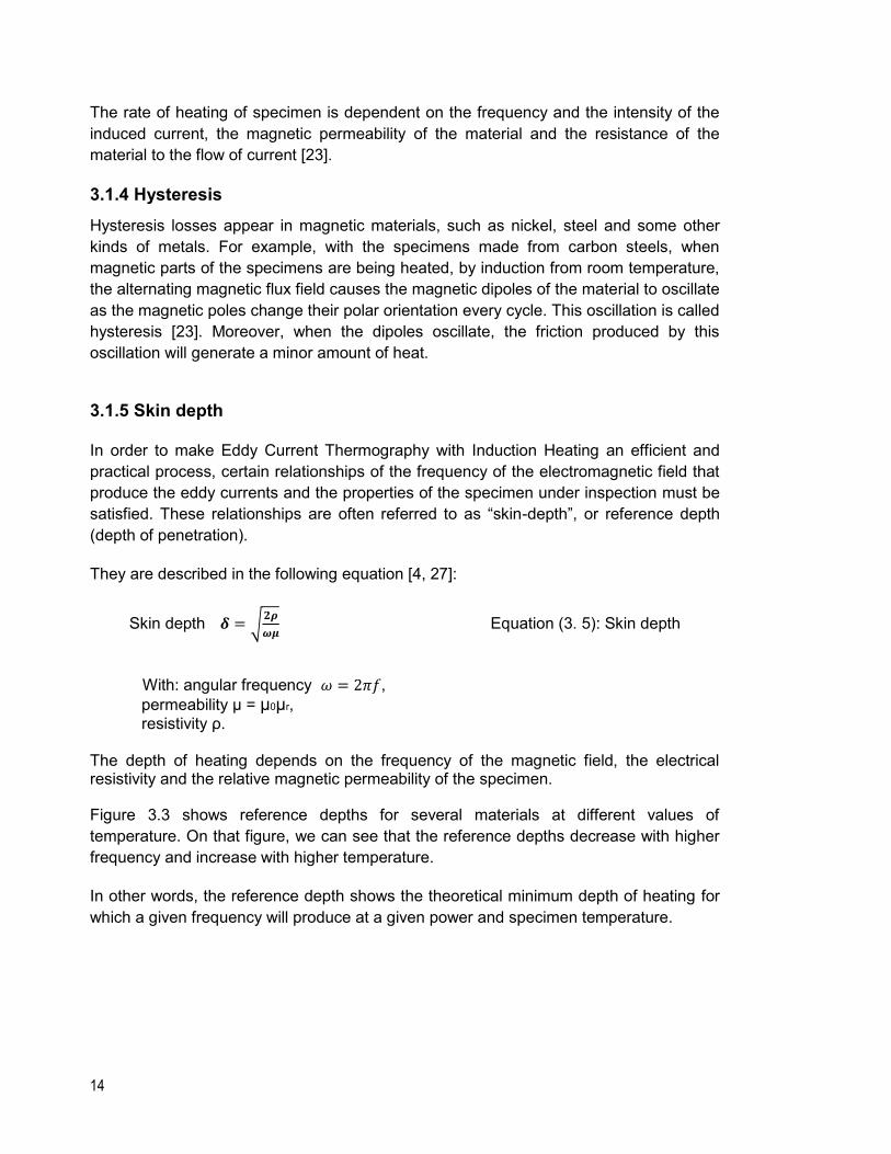
resistivity ρ. The depth of heating depends on the frequency of the magnetic field, the electrical resistivity and the relative magnetic permeability of the specimen.

Figure 3.3 shows reference depths for several materials at different values of

temperature. On that figure, we can see that the reference depths decrease with higher

frequency and increase with higher temperature.

In other words, the reference depth shows the theoretical minimum depth of heating for

which a given frequency will produce at a given power and specimen temperature.

15

Figure 3. 3 : Reference depth for several materials [22]

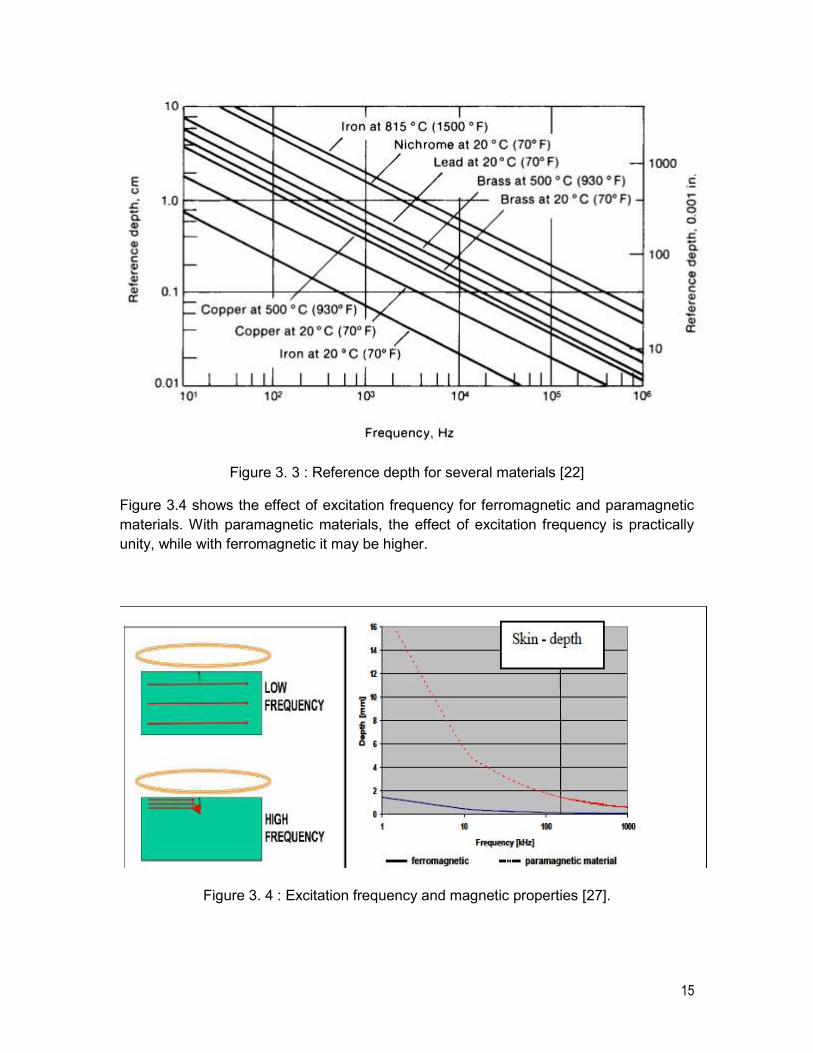
Figure 3.4 shows the effect of excitation frequency for ferromagnetic and paramagnetic

materials. With paramagnetic materials, the effect of excitation frequency is practically

unity, while with ferromagnetic it may be higher.

Figure 3. 4 : Excitation frequency and magnetic properties [27].

16

3.1.5 Heat conduction

The conduction of heat produced by the eddy current is the primary mechanism of heat

flow to the interior of a specimen. Losses due to hysteresis are often ignored in the heat

content calculations for induction processing because of the minor effect [23].

Mathematical analysis of heat transfer may be difficult because of the interaction of the

intense heat produced by the eddy-current heating of the surface. Moreover, the

electrical, thermal, and the properties of most materials show a strong dependence on

temperature and they vary during the heating process.

3.2 Eddy Current Thermography system

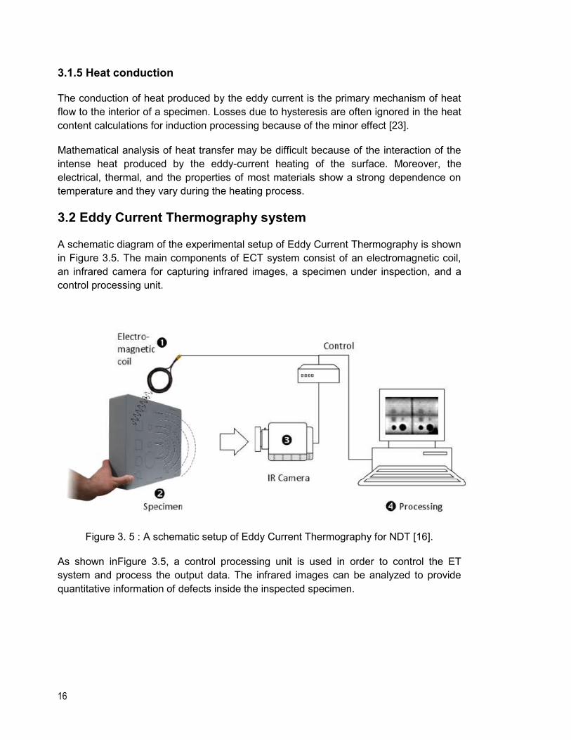
A schematic diagram of the experimental setup of Eddy Current Thermography is shown

in Figure 3.5. The main components of ECT system consist of an electromagnetic coil,

an infrared camera for capturing infrared images, a specimen under inspection, and a

control processing unit.

Figure 3. 5 : A schematic setup of Eddy Current Thermography for NDT [16].

As shown inFigure 3.5, a control processing unit is used in order to control the ET

system and process the output data. The infrared images can be analyzed to provide

quantitative information of defects inside the inspected specimen.

17

3.3 Advantages and limitations

Since ECT is an Infrared Thermography Testing method, it has full advantages and

difficulties (limitations) from IR thermography that have been described in the previous

chapter.

In addition, it has many potential advantages in comparison to heat lamp and sonic

excitation. During the excitation process of the coil, the change of temperature is very

small, and the material under inspection is not damaged, as heating is limited to a few 0C

[29].

Besides, the scanning process and necessity of maintaining a close gap between the

probed surface and the excitation coil might be seen as a drawback of ECT, depending

on the intended application.

3.4 Applications

ECT technique can be used in many industries, in line with other thermographic NDT

techniques, such as sonic thermography, particularly in aerospace industry in which

engine components often show complex geometries [4, 15, 34].

This method is also used to test the coated components in which cracks may occur

under the surface.

18

Chapter 4 Simulations

Today computer simulation has become an essential part of science and engineering. A

computer simulation environment is simply a translation of real world physical-laws into

their virtual form. It would be very helpful to know how much simplification takes place in

the translation stage, then it helps determining the accuracy of the resulting model.

In order to provide efficient solutions for Eddy Current Thermography, it is necessary to

use a numerical simulation software package which has multiphysics capability and can

be utilized to simulate eddy currents and temperature propagation. Moreover, the

numerical software should allow changing the excitation parameters easily [4, 25].

4.1 COMSOL Multiphysic software

It would be ideal to have a simulation environment that included the possibility to add

any physical effect to our model. And that is the design goal of COMSOL.

4.1.1 Introduction

COMSOL Multiphysics® is an integrated environment, a state of the art software for

solving systems of time-dependent or stationary second order in space partial differential

equations (PDEs) in one, two, and three dimensions, by numerical techniques based on

the finite element method (FEM) for the spatial discretization.

COMSOL Multiphysics provides sophisticated and convenient tools for geometric

modeling. For many standard problems, it is possible to use provided templates in order

to hide much of the complex details of modeling by equations. This is really helpful for

the end user.

The step-by-step instruction that is how to model and solve one PDE (in Eddy Current

Thermography) will be described in the appendix 1. In this section, the main components

of a simple simulation are presented in order to provide general information about

modeling in COMSOL Multiphysics.

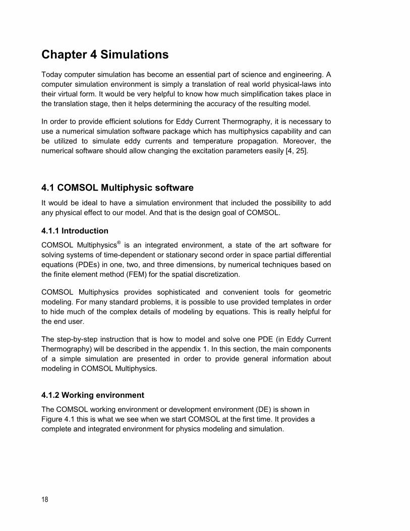
4.1.2 Working environment

The COMSOL working environment or development environment (DE) is shown in

Figure 4.1 this is what we see when we start COMSOL at the first time. It provides a

complete and integrated environment for physics modeling and simulation.

19

Figure 4. 1 : COMSOL integrated development environment.

When we build our model, there are a number of additional windows and widgets that

will be added. These windows are described in the following pages.

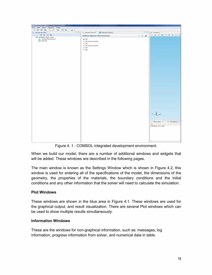
The main window is known as the Settings Window which is shown in Figure 4.2, this

window is used for entering all of the specifications of the model, the dimensions of the

geometry, the properties of the materials, the boundary conditions and the initial

conditions and any other information that the solver will need to calculate the simulation.

Plot Windows

These windows are shown in the blue area in Figure 4.1. These windows are used for

the graphical output, and result visualization. There are several Plot windows which can

be used to show multiple results simultaneously.

Information Windows

These are the windows for non-graphical information, such as: messages, log

information, progress information from solver, and numerical data in table.

20

Figure 4. 2 : Settings window.

Preferences are settings that affect the modeling environment. This window is shown in

Figure 4.3. In this window, we can change settings, such as graphics rendering, number

of displayed digits for Results, or maximum number of CPU to be cores used for

calculations.

Figure 4. 3 : Preference window.

21

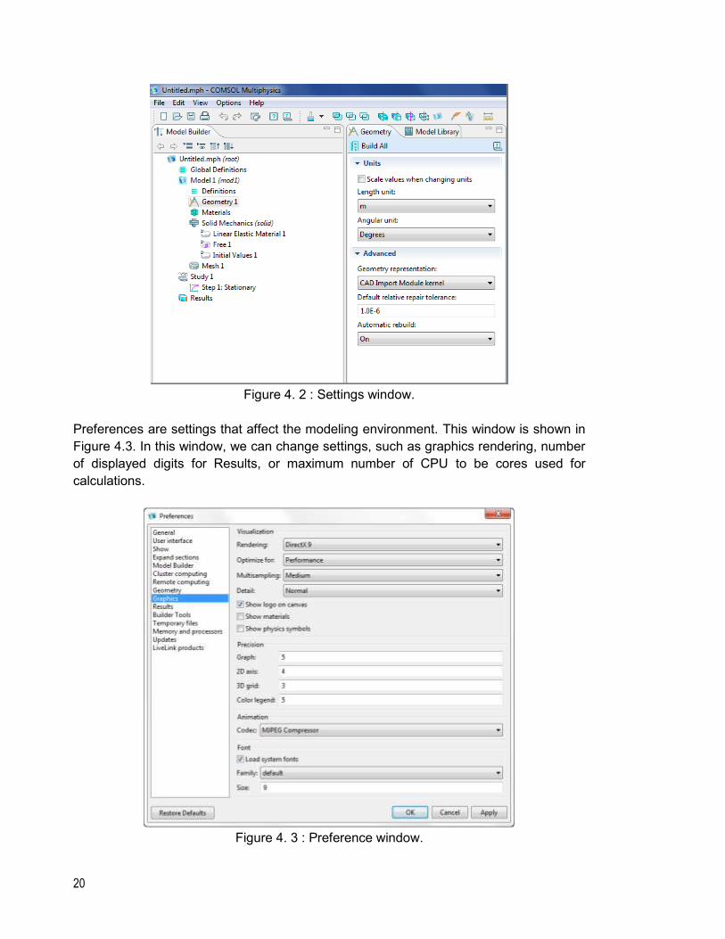
4.1.3 The Model Builder and the Model Tree

The Model Builder is a tool where we can define the model, the analysis of results, and

the reports. These works are done by building a Model Tree.

When we start building a tree, a default Model Tree will be added. All of the nodes in the

default Model Tree are top-level parent nodes. A Model Tree always consists of a Root

node, a Global Definitions node and a Results node as shown in Figure 4.4.

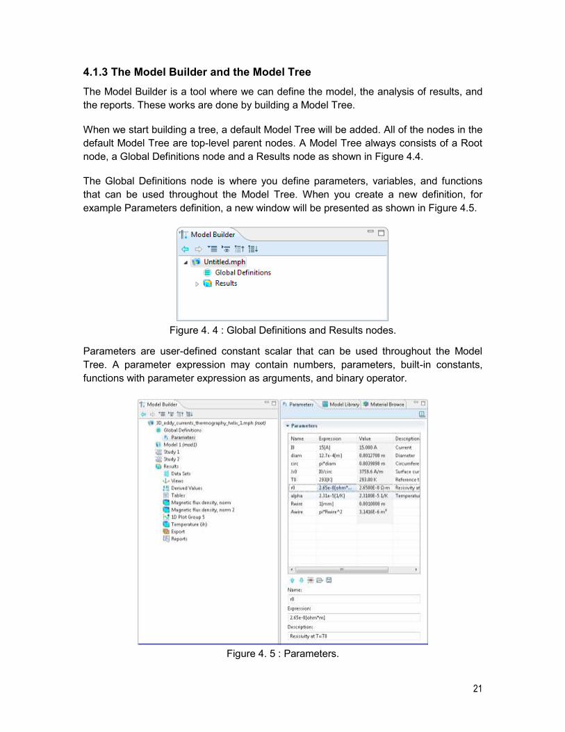
The Global Definitions node is where you define parameters, variables, and functions

that can be used throughout the Model Tree. When you create a new definition, for

example Parameters definition, a new window will be presented as shown in Figure 4.5.

Figure 4. 4 : Global Definitions and Results nodes.

Parameters are user-defined constant scalar that can be used throughout the Model

Tree. A parameter expression may contain numbers, parameters, built-in constants,

functions with parameter expression as arguments, and binary operator.

Figure 4. 5 : Parameters.

22

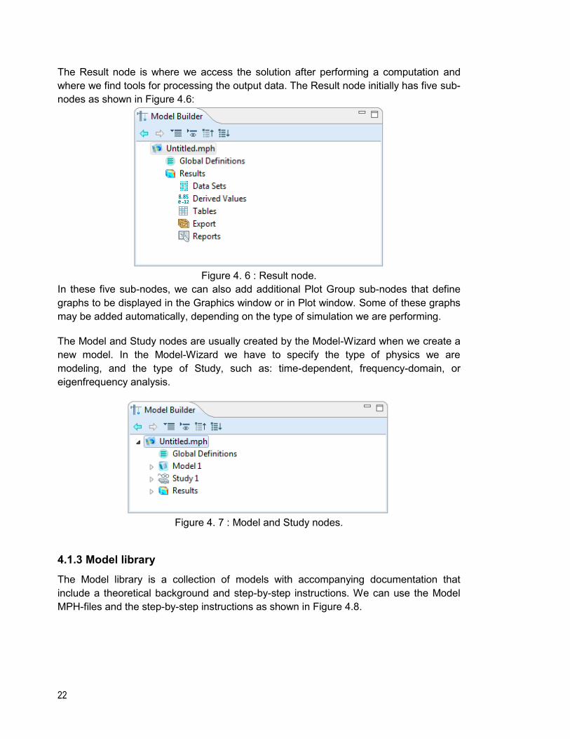
The Result node is where we access the solution after performing a computation and

where we find tools for processing the output data. The Result node initially has five sub-

nodes as shown in Figure 4.6:

Figure 4. 6 : Result node.

In these five sub-nodes, we can also add additional Plot Group sub-nodes that define

graphs to be displayed in the Graphics window or in Plot window. Some of these graphs

may be added automatically, depending on the type of simulation we are performing.

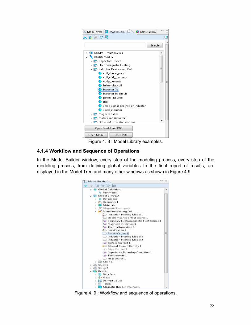
The Model and Study nodes are usually created by the Model-Wizard when we create a

new model. In the Model-Wizard we have to specify the type of physics we are

modeling, and the type of Study, such as: time-dependent, frequency-domain, or

eigenfrequency analysis.

Figure 4. 7 : Model and Study nodes.

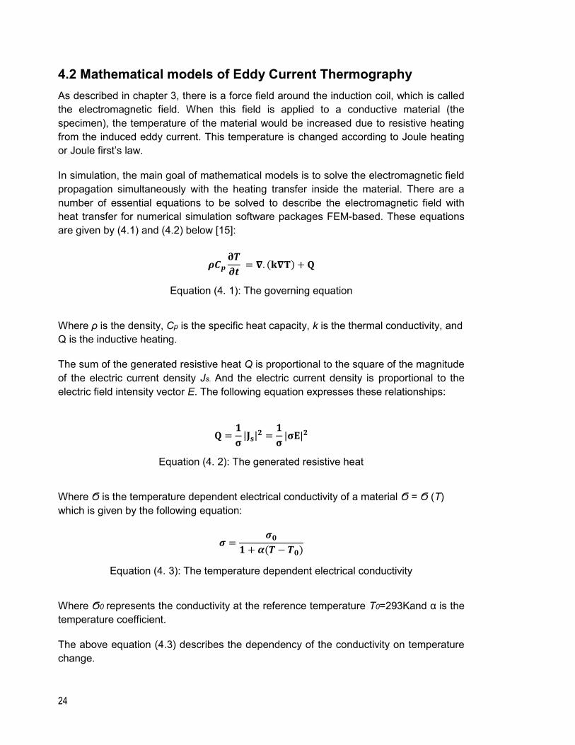
4.1.3 Model library

The Model library is a collection of models with accompanying documentation that

include a theoretical background and step-by-step instructions. We can use the Model

MPH-files and the step-by-step instructions as shown in Figure 4.8.

23

Figure 4. 8 : Model Library examples.

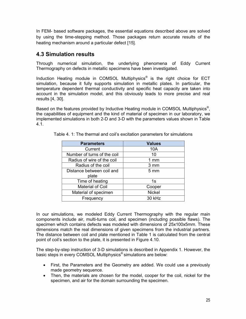
4.1.4 Workflow and Sequence of Operations

In the Model Builder window, every step of the modeling process, every step of the

modeling process, from defining global variables to the final report of results, are

displayed in the Model Tree and many other windows as shown in Figure 4.9

Figure 4. 9 : Workflow and sequence of operations.

24

4.2 Mathematical models of Eddy Current Thermography

As described in chapter 3, there is a force field around the induction coil, which is called

the electromagnetic field. When this field is applied to a conductive material (the

specimen), the temperature of the material would be increased due to resistive heating

from the induced eddy current. This temperature is changed according to Joule heating

or Joule first’s law.

In simulation, the main goal of mathematical models is to solve the electromagnetic field

propagation simultaneously with the heating transfer inside the material. There are a

number of essential equations to be solved to describe the electromagnetic field with

heat transfer for numerical simulation software packages FEM-based. These equations

are given by (4.1) and (4.2) below [15]:

( )

Equation (4. 1): The governing equation

Where ρ is the density, Cp is the specific heat capacity, k is the thermal conductivity, and

Q is the inductive heating.

The sum of the generated resistive heat Q is proportional to the square of the magnitude

of the electric current density Js. And the electric current density is proportional to the

electric field intensity vector E. The following equation expresses these relationships:

| |

| |

Equation (4. 2): The generated resistive heat

Where Ϭ is the temperature dependent electrical conductivity of a material Ϭ = Ϭ (T)

which is given by the following equation:

( )

Equation (4. 3): The temperature dependent electrical conductivity

Where Ϭ0 represents the conductivity at the reference temperature T0=293Kand α is the

temperature coefficient.

The above equation (4.3) describes the dependency of the conductivity on temperature

change.

25

In FEM- based software packages, the essential equations described above are solved

by using the time-stepping method. Those packages return accurate results of the

heating mechanism around a particular defect [15].

4.3 Simulation results

Through numerical simulation, the underlying phenomena of Eddy Current Thermography on defects in metallic specimens have been investigated.

Induction Heating module in COMSOL Multiphysics® is the right choice for ECT simulation, because it fully supports simulation in metallic plates. In particular, the temperature dependent thermal conductivity and specific heat capacity are taken into account in the simulation model, and this obviously leads to more precise and real results [4, 30].

Based on the features provided by Inductive Heating module in COMSOL Multiphysics®, the capabilities of equipment and the kind of material of specimen in our laboratory, we implemented simulations in both 2-D and 3-D with the parameters values shown in Table 4.1.

Table 4. 1: The thermal and coil’s excitation parameters for simulations

Parameters Values

Current 10A

Number of turns of the coil 10

Radius of wire of the coil 1 mm

Radius of the coil 3 mm

Distance between coil and plate

5 mm

Time of heating 1s

Material of Coil Cooper

Material of specimen Nickel

Frequency 30 kHz

In our simulations, we modeled Eddy Current Thermography with the regular main components include air, multi-turns coil, and specimen (including possible flaws). The specimen which contains defects was modeled with dimensions of 25x100x5mm. These dimensions match the real dimensions of given specimens from the industrial partners. The distance between coil and plate mentioned in Table 1 is calculated from the central point of coil’s section to the plate, it is presented in Figure 4.10.

The step-by-step instruction of 3-D simulations is described in Appendix 1. However, the basic steps in every COMSOL Multiphysics® simulations are below:

First, the Parameters and the Geometry are added. We could use a previously made geometry sequence.

Then, the materials are chosen for the model, cooper for the coil, nickel for the specimen, and air for the domain surrounding the specimen.

26

The physical Induction Heating set-up shows the equations and boundary conditions used to solve the model.

Finally the mesh is set up and the results are solved.

The results of both 2-D and 3-D simulations are presented in the next sections.

4.3.1 2-D simulation results

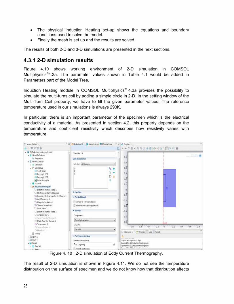
Figure 4.10 shows working environment of 2-D simulation in COMSOL

Multiphysics®4.3a. The parameter values shown in Table 4.1 would be added in

Parameters part of the Model Tree.

Induction Heating module in COMSOL Multiphysics® 4.3a provides the possibility to

simulate the multi-turns coil by adding a simple circle in 2-D. In the setting window of the

Multi-Turn Coil property, we have to fill the given parameter values. The reference

temperature used in our simulations is always 293K.

In particular, there is an important parameter of the specimen which is the electrical

conductivity of a material. As presented in section 4.2, this property depends on the

temperature and coefficient resistivity which describes how resistivity varies with

temperature.

Figure 4. 10 : 2-D simulation of Eddy Current Thermography.

The result of 2-D simulation is shown in Figure 4.11. We do not see the temperature

distribution on the surface of specimen and we do not know how that distribution affects

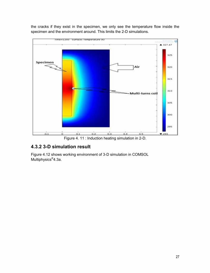
27

the cracks if they exist in the specimen, we only see the temperature flow inside the

specimen and the environment around. This limits the 2-D simulations.

Figure 4. 11 : Induction heating simulation in 2-D.

4.3.2 3-D simulation result

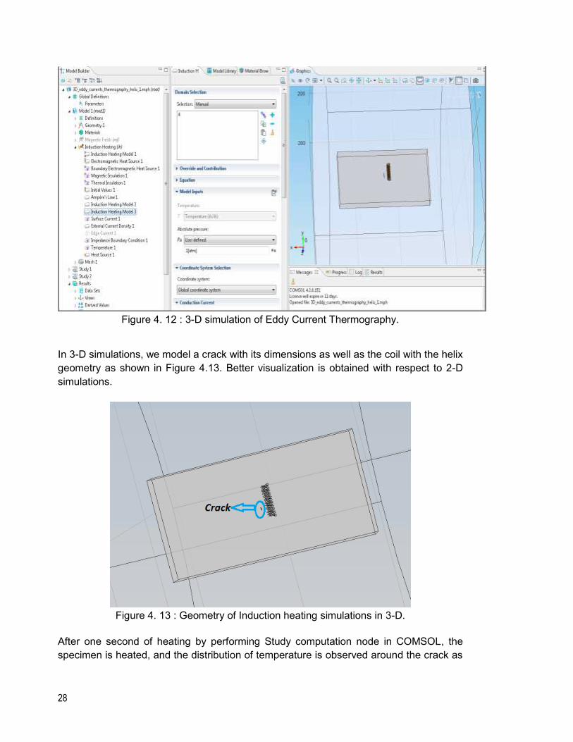
Figure 4.12 shows working environment of 3-D simulation in COMSOL

Multiphysics®4.3a.

28

Figure 4. 12 : 3-D simulation of Eddy Current Thermography.

In 3-D simulations, we model a crack with its dimensions as well as the coil with the helix

geometry as shown in Figure 4.13. Better visualization is obtained with respect to 2-D

simulations.

Figure 4. 13 : Geometry of Induction heating simulations in 3-D.

After one second of heating by performing Study computation node in COMSOL, the

specimen is heated, and the distribution of temperature is observed around the crack as

29

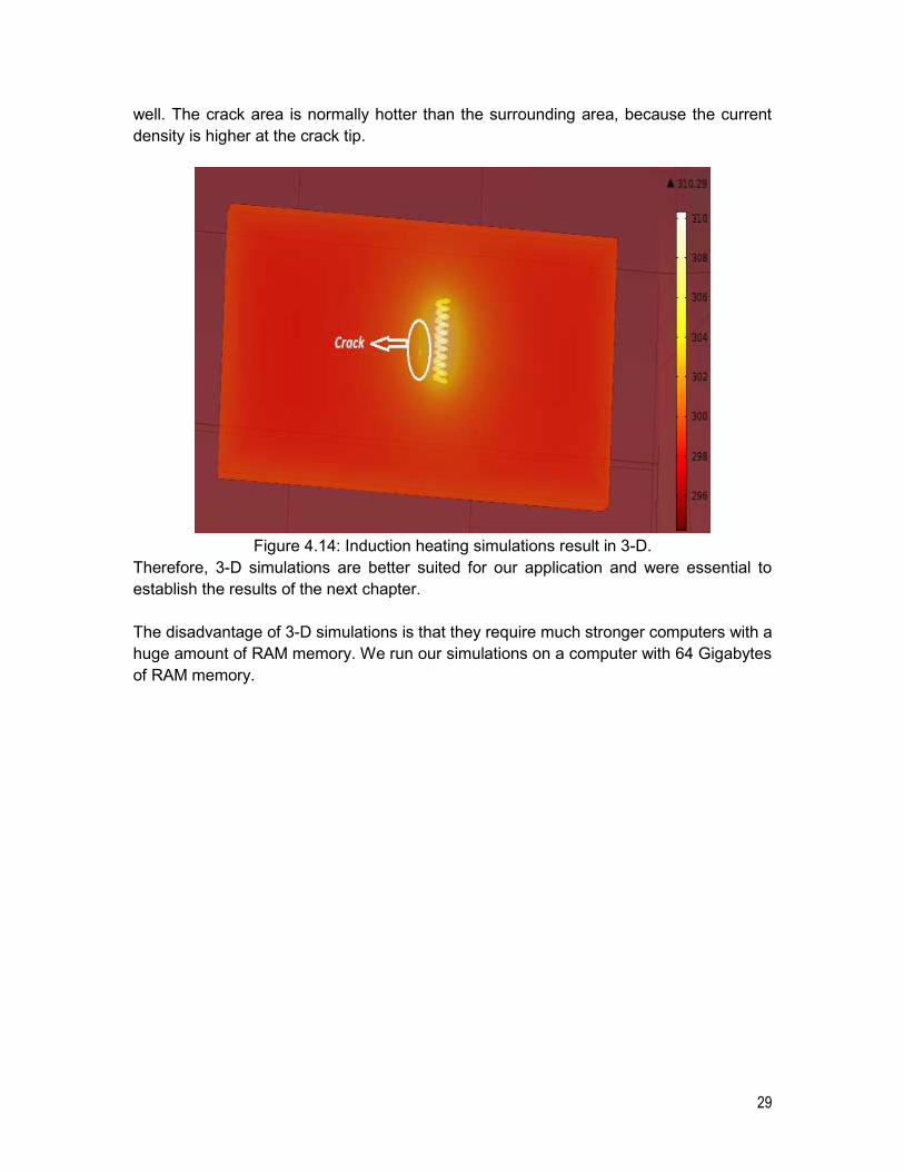
well. The crack area is normally hotter than the surrounding area, because the current

density is higher at the crack tip.

Figure 4.14: Induction heating simulations result in 3-D.

Therefore, 3-D simulations are better suited for our application and were essential to

establish the results of the next chapter.

The disadvantage of 3-D simulations is that they require much stronger computers with a

huge amount of RAM memory. We run our simulations on a computer with 64 Gigabytes

of RAM memory.

30

Chapter 5 Equipment and experimentation

parameters

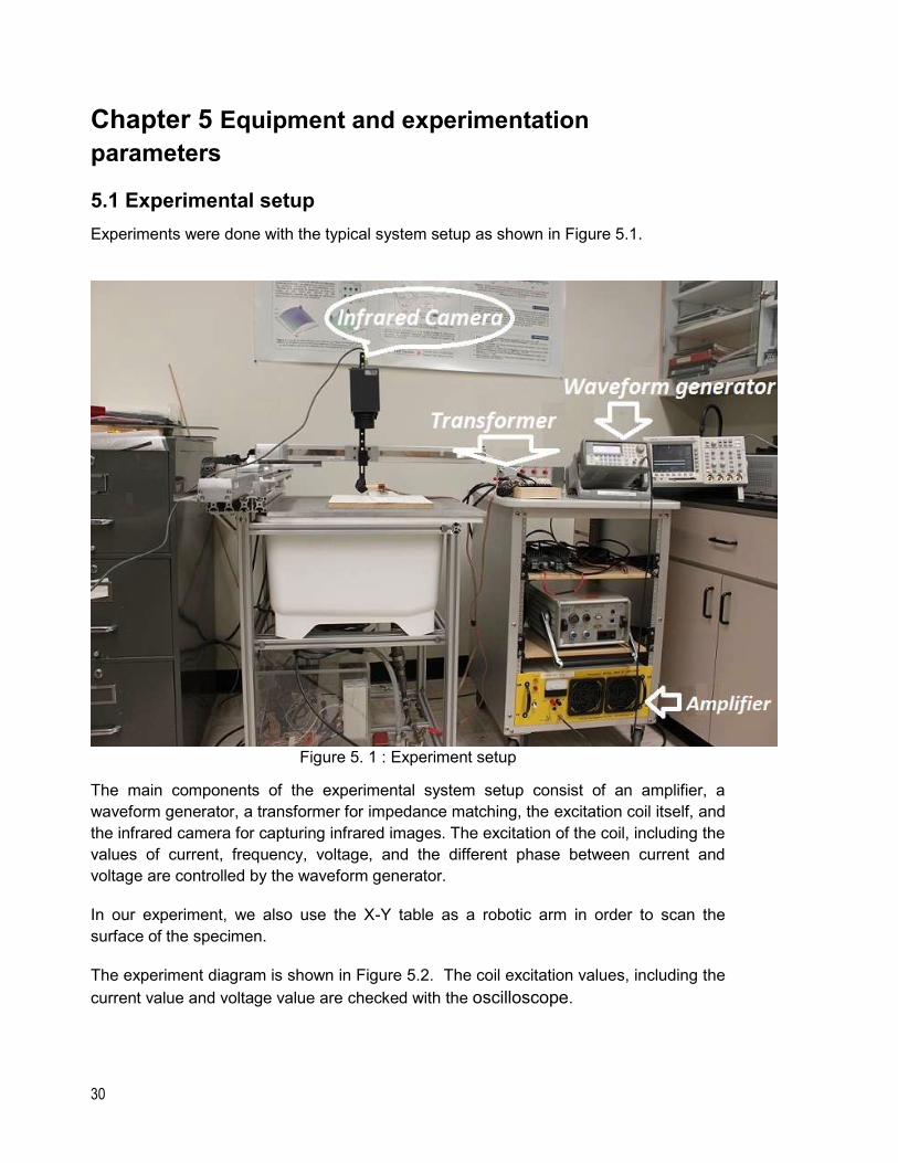
5.1 Experimental setup

Experiments were done with the typical system setup as shown in Figure 5.1.

Figure 5. 1 : Experiment setup

The main components of the experimental system setup consist of an amplifier, a

waveform generator, a transformer for impedance matching, the excitation coil itself, and

the infrared camera for capturing infrared images. The excitation of the coil, including the

values of current, frequency, voltage, and the different phase between current and

voltage are controlled by the waveform generator.

In our experiment, we also use the X-Y table as a robotic arm in order to scan the

surface of the specimen.

The experiment diagram is shown in Figure 5.2. The coil excitation values, including the

current value and voltage value are checked with the oscilloscope.

31

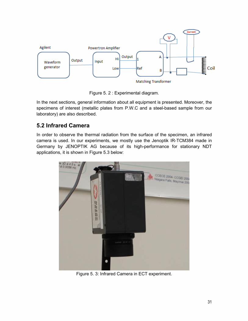
Figure 5. 2 : Experimental diagram.

In the next sections, general information about all equipment is presented. Moreover, the

specimens of interest (metallic plates from P.W.C and a steel-based sample from our

laboratory) are also described.

5.2 Infrared Camera

In order to observe the thermal radiation from the surface of the specimen, an infrared

camera is used. In our experiments, we mostly use the Jenoptik IR-TCM384 made in

Germany by JENOPTIK AG because of its high-performance for stationary NDT

applications, it is shown in Figure 5.3 below:

Figure 5. 3: Infrared Camera in ECT experiment.

32

This camera operates in the spectral range (SR) 7.5 to 14 µm. Technical specifications

of this kind of camera are presented in Appendix 4. However, there are some features

that make it widely used: high frame rate (50/60 Hz), lightweight and compact design,

wide measuring range temperature standard (WMRTS).

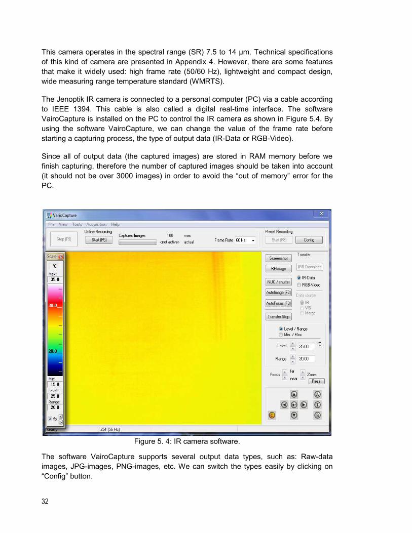
The Jenoptik IR camera is connected to a personal computer (PC) via a cable according

to IEEE 1394. This cable is also called a digital real-time interface. The software

VairoCapture is installed on the PC to control the IR camera as shown in Figure 5.4. By

using the software VairoCapture, we can change the value of the frame rate before

starting a capturing process, the type of output data (IR-Data or RGB-Video).

Since all of output data (the captured images) are stored in RAM memory before we

finish capturing, therefore the number of captured images should be taken into account

(it should not be over 3000 images) in order to avoid the “out of memory” error for the

PC.

Figure 5. 4: IR camera software.

The software VairoCapture supports several output data types, such as: Raw-data

images, JPG-images, PNG-images, etc. We can switch the types easily by clicking on

“Config” button.

33

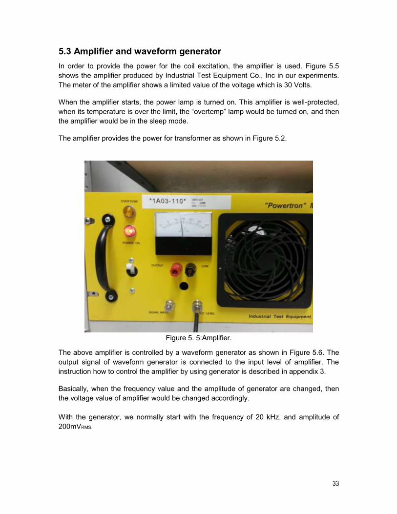
5.3 Amplifier and waveform generator

In order to provide the power for the coil excitation, the amplifier is used. Figure 5.5

shows the amplifier produced by Industrial Test Equipment Co., Inc in our experiments.

The meter of the amplifier shows a limited value of the voltage which is 30 Volts.

When the amplifier starts, the power lamp is turned on. This amplifier is well-protected,

when its temperature is over the limit, the “overtemp” lamp would be turned on, and then

the amplifier would be in the sleep mode.

The amplifier provides the power for transformer as shown in Figure 5.2.

Figure 5. 5:Amplifier.

The above amplifier is controlled by a waveform generator as shown in Figure 5.6. The

output signal of waveform generator is connected to the input level of amplifier. The

instruction how to control the amplifier by using generator is described in appendix 3.

Basically, when the frequency value and the amplitude of generator are changed, then

the voltage value of amplifier would be changed accordingly.

With the generator, we normally start with the frequency of 20 kHz, and amplitude of

200mVRMS.

34

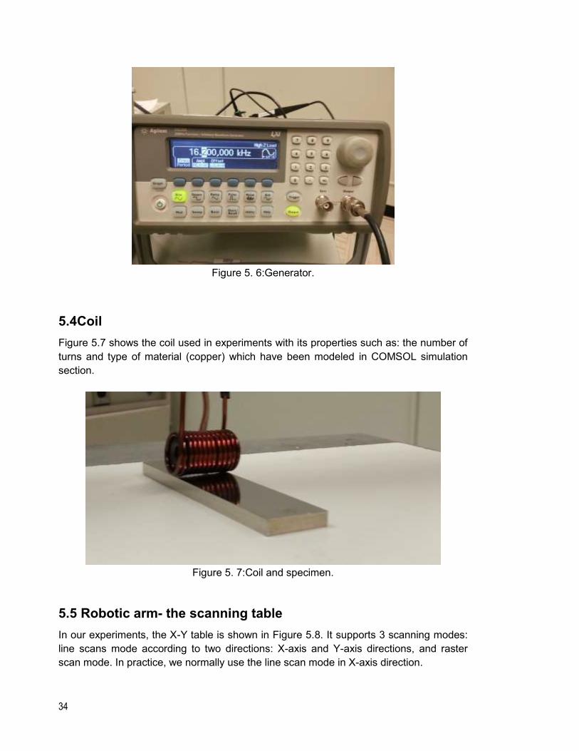
Figure 5. 6:Generator.

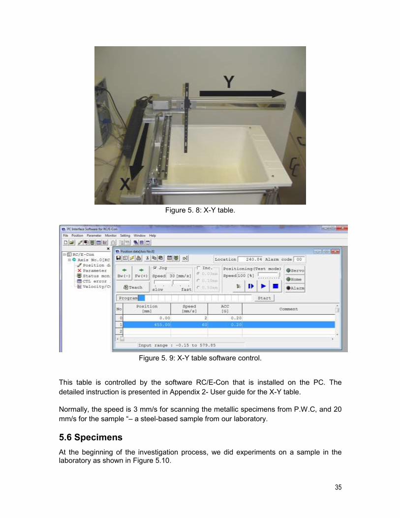
5.4Coil

Figure 5.7 shows the coil used in experiments with its properties such as: the number of

turns and type of material (copper) which have been modeled in COMSOL simulation

section.

Figure 5. 7:Coil and specimen.

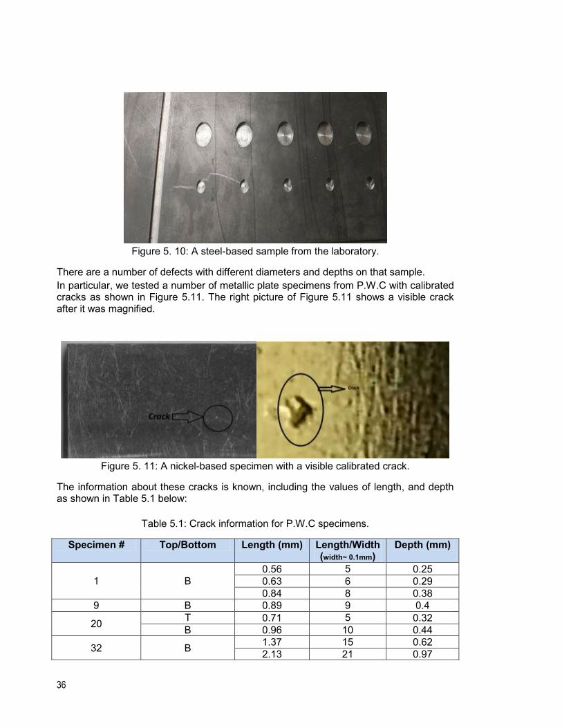
5.5 Robotic arm- the scanning table

In our experiments, the X-Y table is shown in Figure 5.8. It supports 3 scanning modes:

line scans mode according to two directions: X-axis and Y-axis directions, and raster

scan mode. In practice, we normally use the line scan mode in X-axis direction.

35

Figure 5. 8: X-Y table.

Figure 5. 9: X-Y table software control.

This table is controlled by the software RC/E-Con that is installed on the PC. The

detailed instruction is presented in Appendix 2- User guide for the X-Y table.

Normally, the speed is 3 mm/s for scanning the metallic specimens from P.W.C, and 20

mm/s for the sample “– a steel-based sample from our laboratory.

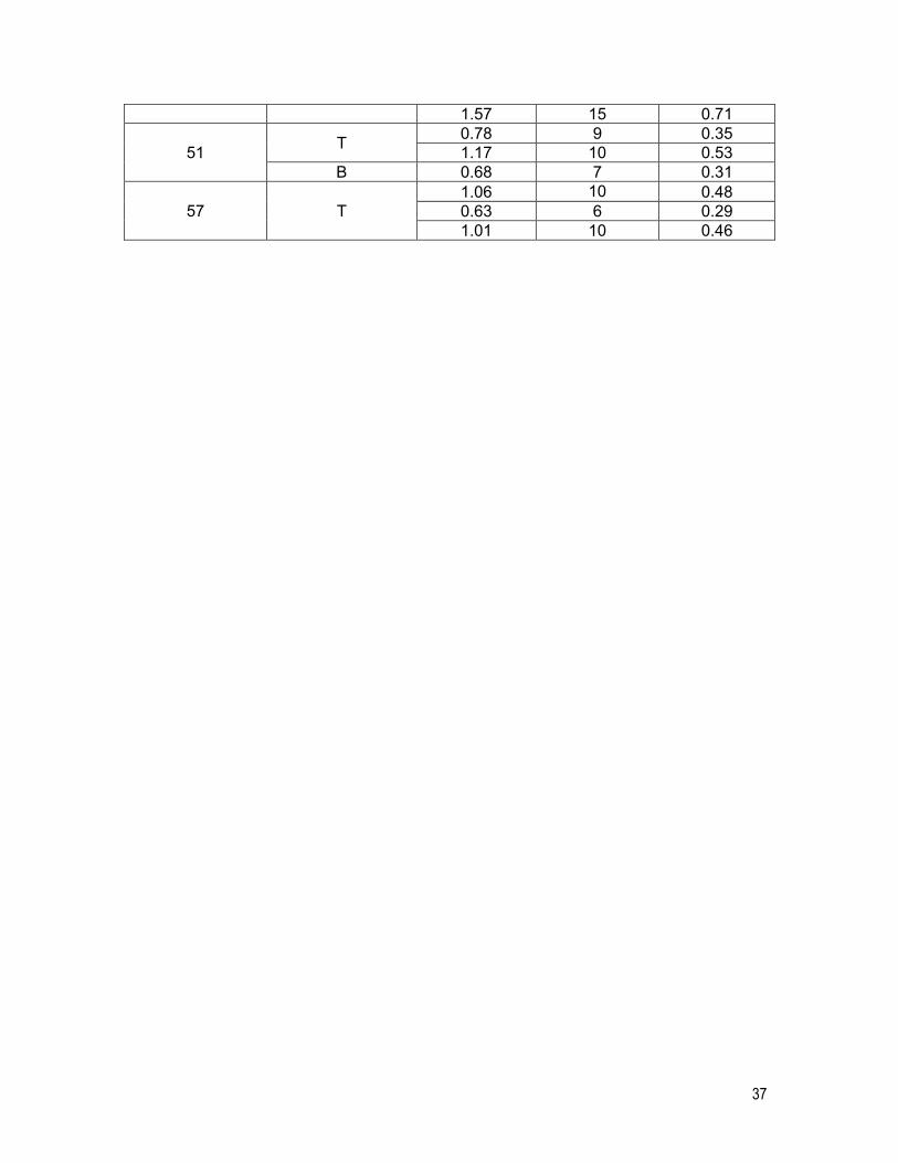
5.6 Specimens

At the beginning of the investigation process, we did experiments on a sample in the laboratory as shown in Figure 5.10.

36

Figure 5. 10: A steel-based sample from the laboratory.

There are a number of defects with different diameters and depths on that sample.

In particular, we tested a number of metallic plate specimens from P.W.C with calibrated cracks as shown in Figure 5.11. The right picture of Figure 5.11 shows a visible crack after it was magnified.

Figure 5. 11: A nickel-based specimen with a visible calibrated crack.

The information about these cracks is known, including the values of length, and depth as shown in Table 5.1 below:

Table 5.1: Crack information for P.W.C specimens.

Specimen # Top/Bottom Length (mm) Length/Width (width~ 0.1mm)

Depth (mm)

1 B

0.56 5 0.25

0.63 6 0.29

0.84 8 0.38

9 B 0.89 9 0.4

20 T 0.71 5 0.32

B 0.96 10 0.44

32 B 1.37 15 0.62

2.13 21 0.97

37

1.57 15 0.71

51 T

0.78 9 0.35

1.17 10 0.53

B 0.68 7 0.31

57 T

1.06 10 0.48

0.63 6 0.29

1.01 10 0.46

38

Chapter 6 Results

6.1 Crack detection limit

In this section, we would like to propose a new approach based on 3-D simulation

results obtained in chapter 4.

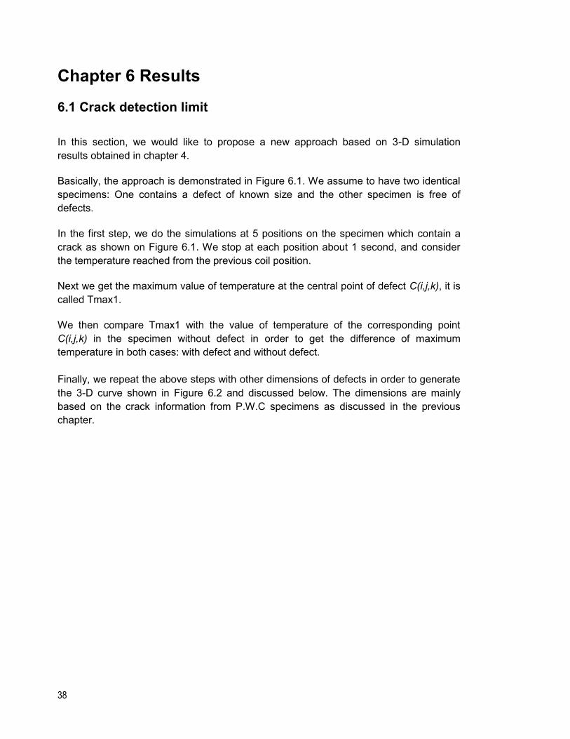
Basically, the approach is demonstrated in Figure 6.1. We assume to have two identical

specimens: One contains a defect of known size and the other specimen is free of

defects.

In the first step, we do the simulations at 5 positions on the specimen which contain a

crack as shown on Figure 6.1. We stop at each position about 1 second, and consider

the temperature reached from the previous coil position.

Next we get the maximum value of temperature at the central point of defect C(i,j,k), it is

called Tmax1.

We then compare Tmax1 with the value of temperature of the corresponding point

C(i,j,k) in the specimen without defect in order to get the difference of maximum

temperature in both cases: with defect and without defect.

Finally, we repeat the above steps with other dimensions of defects in order to generate

the 3-D curve shown in Figure 6.2 and discussed below. The dimensions are mainly

based on the crack information from P.W.C specimens as discussed in the previous

chapter.

39

Figure 6. 1: The approach for crack detection limit.

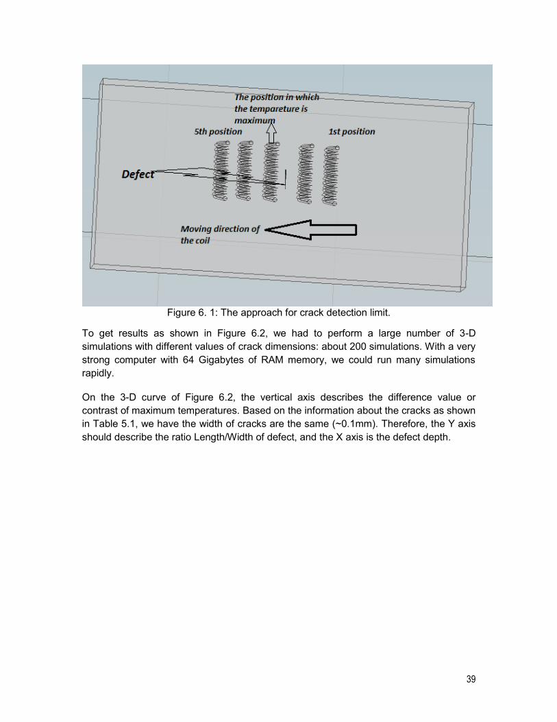
To get results as shown in Figure 6.2, we had to perform a large number of 3-D

simulations with different values of crack dimensions: about 200 simulations. With a very

strong computer with 64 Gigabytes of RAM memory, we could run many simulations

rapidly.

On the 3-D curve of Figure 6.2, the vertical axis describes the difference value or

contrast of maximum temperatures. Based on the information about the cracks as shown

in Table 5.1, we have the width of cracks are the same (~0.1mm). Therefore, the Y axis

should describe the ratio Length/Width of defect, and the X axis is the defect depth.

40

Figure 6. 2: The 3-D curve of crack detection limit (from simulated data).

6.2 Experimental results

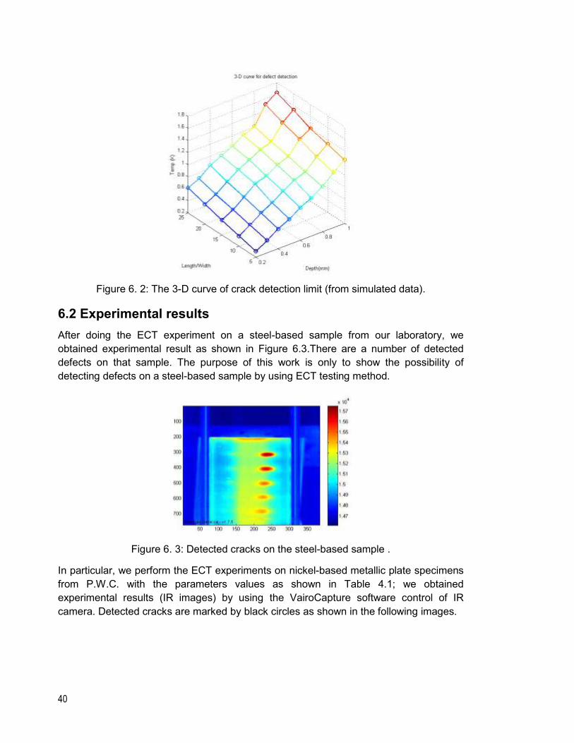
After doing the ECT experiment on a steel-based sample from our laboratory, we

obtained experimental result as shown in Figure 6.3.There are a number of detected

defects on that sample. The purpose of this work is only to show the possibility of

detecting defects on a steel-based sample by using ECT testing method.

Figure 6. 3: Detected cracks on the steel-based sample .

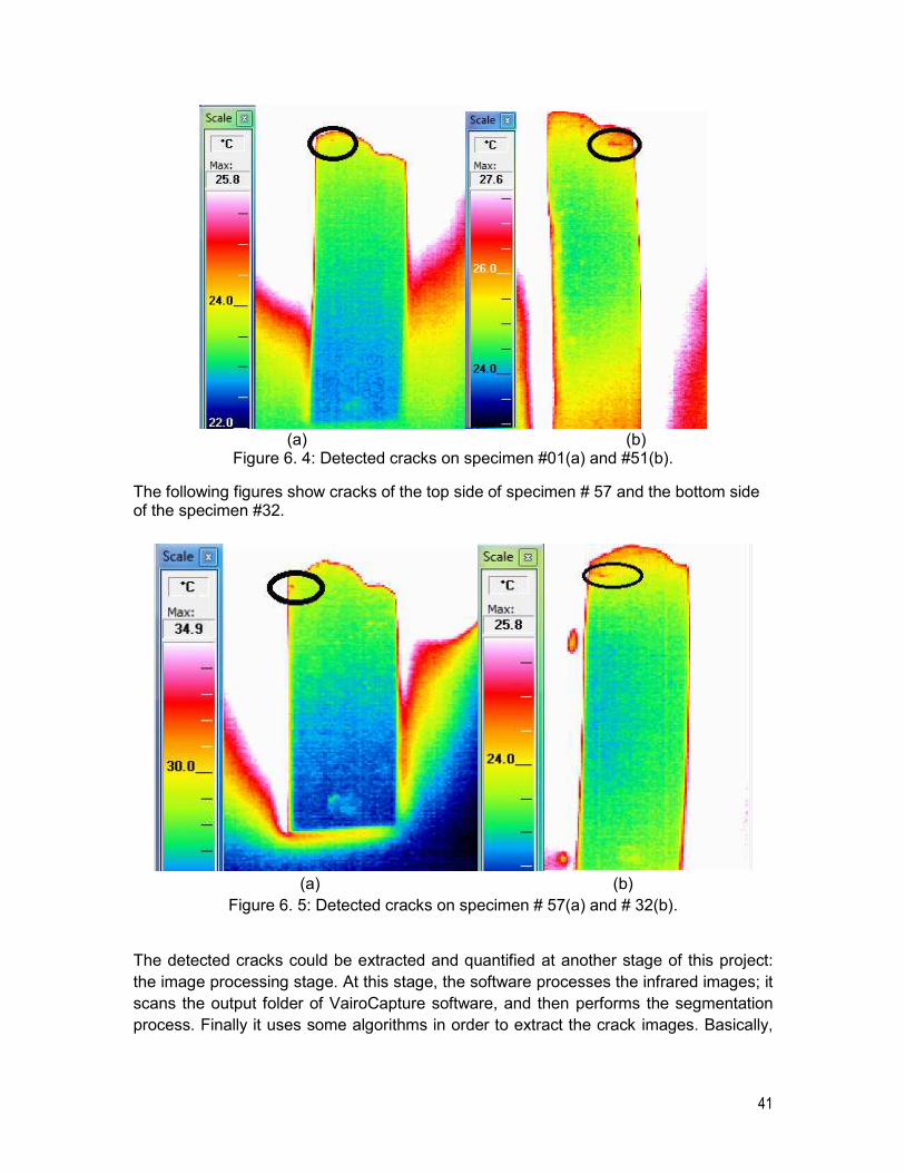
In particular, we perform the ECT experiments on nickel-based metallic plate specimens

from P.W.C. with the parameters values as shown in Table 4.1; we obtained

experimental results (IR images) by using the VairoCapture software control of IR

camera. Detected cracks are marked by black circles as shown in the following images.

41

(a) (b)

Figure 6. 4: Detected cracks on specimen #01(a) and #51(b).

The following figures show cracks of the top side of specimen # 57 and the bottom side of the specimen #32.

(a) (b)

Figure 6. 5: Detected cracks on specimen # 57(a) and # 32(b).

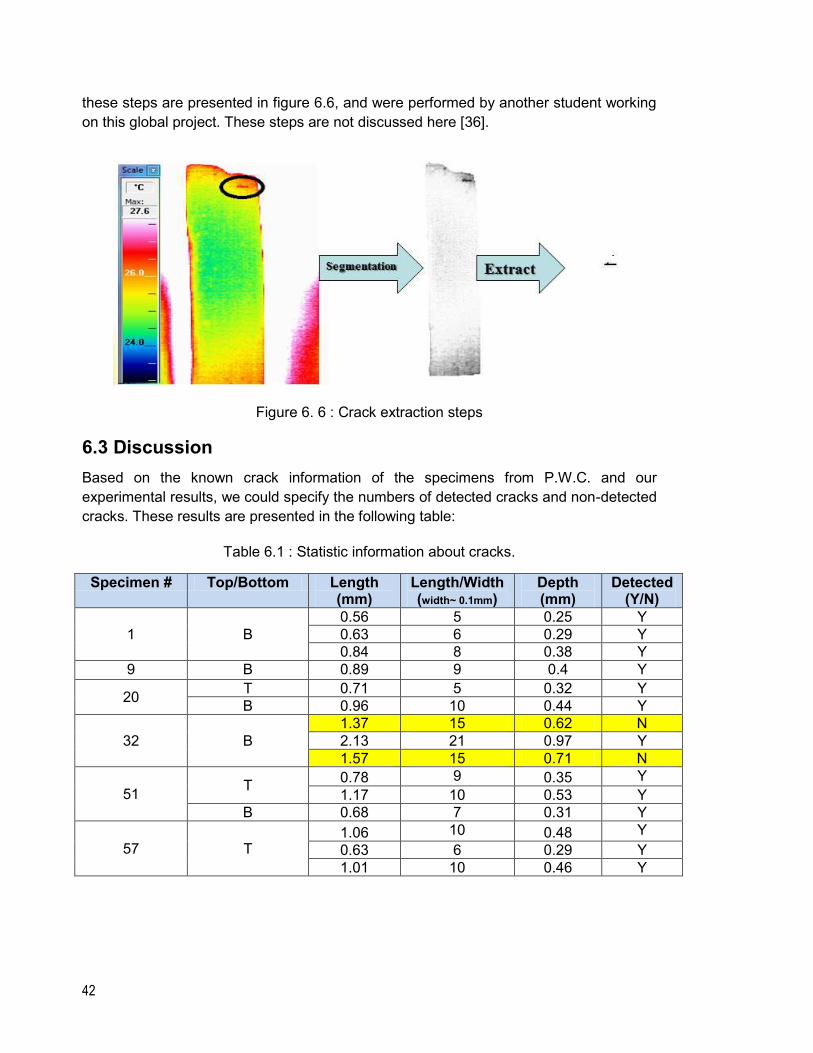
The detected cracks could be extracted and quantified at another stage of this project:

the image processing stage. At this stage, the software processes the infrared images; it

scans the output folder of VairoCapture software, and then performs the segmentation

process. Finally it uses some algorithms in order to extract the crack images. Basically,

42

these steps are presented in figure 6.6, and were performed by another student working

on this global project. These steps are not discussed here [36].

Figure 6. 6 : Crack extraction steps

6.3 Discussion

Based on the known crack information of the specimens from P.W.C. and our

experimental results, we could specify the numbers of detected cracks and non-detected

cracks. These results are presented in the following table:

Table 6.1 : Statistic information about cracks.

Specimen # Top/Bottom Length (mm)

Length/Width (width~ 0.1mm)

Depth (mm)

Detected (Y/N)

1 B

0.56 5 0.25 Y

0.63 6 0.29 Y

0.84 8 0.38 Y

9 B 0.89 9 0.4 Y

20 T 0.71 5 0.32 Y

B 0.96 10 0.44 Y

32 B

1.37 15 0.62 N

2.13 21 0.97 Y

1.57 15 0.71 N

51 T

0.78 9 0.35 Y

1.17 10 0.53 Y

B 0.68 7 0.31 Y

57 T 1.06 10 0.48 Y

0.63 6 0.29 Y

1.01 10 0.46 Y

43

There are two non-detected cracks in our experiments on given specimens. The reason

for this is because the direction of these cracks is not perpendicular to the moving

direction of the coil. Therefore, the surface discontinuities are not detected in this case

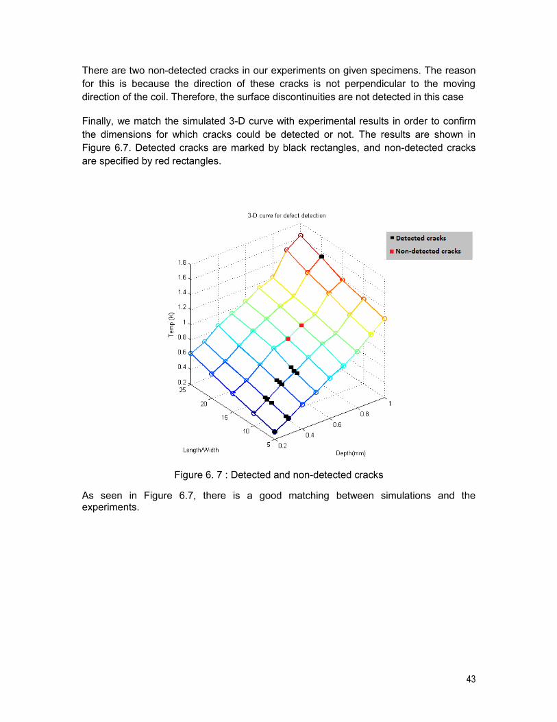
Finally, we match the simulated 3-D curve with experimental results in order to confirm

the dimensions for which cracks could be detected or not. The results are shown in

Figure 6.7. Detected cracks are marked by black rectangles, and non-detected cracks

are specified by red rectangles.

Figure 6. 7 : Detected and non-detected cracks

As seen in Figure 6.7, there is a good matching between simulations and the experiments.

44

Chapter 7 Conclusion

Simulations and experiments of Eddy Current Thermography techniques for non-

destructive characterization of metallic materials have been investigated in this thesis.

In order to optimize the experiments, Induction Heating module of COMSOL

Multiphysics® software was used to model the ECT testing method, in both cases: 2-D

and 3-D simulations were performed, since they enable simulation of metallic plates.

The limitations of 2-D simulation were discussed. It is better to use 3-D simulations. This

type of simulation provided some advantages; it showed how temperature propagates

under the surface, and what happened when the temperature flow meets cracks.

A new approach based on the temperature reached at the central point of defects

according to different positions of the coil has been exposed in order to generate a 3-D

curve. This curve was generated by performing many simulations with a strong

computer. It enables to establish the limit of crack detection for ECT in nickel-based

specimens or other kind of metallic specimen as well.

Experimental tests were done on many specimens from P.W.C in order to verify the

crack detection limit and to establish the possibility of this NDT inspection technique.

Moreover, at the end of my research, in this project, I published a conference paper to

The American Society for Nondestructive Testing 22nd Research Symposium 2013 with

the following title “Crack Detection Limit in Eddy Current Thermography” [4].

The other important parts of this thesis are the step by step instruction guide to establish

Eddy Current Thermography simulations and experiments. They are presented in

Appendix 1 and Appendix 3.

Future work could be done on matching the dimensions of real cracks to establish a link

with experimental infrared signatures.

45

Bibliography [1] Project description, “Automated Non Destructive Testing for the Aerospace Industry”,

CRIAQ MANU-418, May 12, 2010.

[2] Clemente Ibarra-Castanedo, Marc Genest, Jean-Marc Piau, StéphaneGuibert,

Abdelhakim Bendada and Xavier P.V. Maldague, “Chapter 14: Active Infrared

Thermography techniques for the nondestructive testing of materials”, Ultrasonic and

Advanced Methods for Nondestructive Testing and Material Characterization, C.H.

Chen Ed., p325-348, 2006.

[3] Reza ShojaGhiass, YuxiaDuan, KiraPaycheva, Xavier Maldague, “Inspection of

glass fiber reinforced plastic (GFRP) using Near/Shortwave Infrared and

Ultrasound/Optical excitation Thermography”, Smart Materials, Structures and NDT

in Aerospace Conference, NDT in Canada, Montreal Quebec Canada, November

2011.

[4] P.Tran-Gia, X.Maldague, L.Birglen, “Crack Detection Limit in Eddy Current

Thermography”, ASNT 22th Research Symposium, Memphis Tennessee, March,

2013.

[5] Xavier P.V. Maldague., “Theory and Practice of Infrared Technology for

Nondestructive Testing”, John Wiley- Interscience, 2001.

[6] Clemente Ibarra-Castanedo, Marc Genest, Jean-Marc Piau, Stéphane Guibert,

Abdelhakim Bendada and Xavier P.V. Maldague, “Inspection of aerospace materials

by pulsed thermography, lock-in thermography and vibrothermography: A

comparative study”, SPIE, ThermosenseXXIX, 2007.

[7] Clemente Ibarra-Castanedo, Mirela Susa, Matthieu Klein, Marc Grenier, Jean-Marc

Piau, Wael Ben Larby, Abdelhakim Bendada and Xavier Maldague, “Infrared

Thermography: principle and applications to aircraft materials”, Nondestructive

Testing Journal, 2008.

[8] Xavier P.V. Maldague., “Introduction to NDT by Active Infrared Thermography”,

Material Evaluation, 2002.

[9] L.D. Favro and X. Han, "Thermal Wave Materials Characterization and Thermal

Wave Imaging," Processing and Manufacuring, ASNT TONES, pp. 399-415,1998.

[10] G. Busse and A. Rosencwaig, "Subsurface Imaging with Photoacoustics," Appl.

Phys. Lett., vol. 36, pp. 815-816, 1980.

[11] R. L. Thomas, et al., "Subsurface Flaw Detection in Metals by Photoacustic

Microscopy" J. Appl. Phys, vol. 51, pp. 1152-1156, 1980.

46

[12] P. O. Moore ed., X. Maldague technical ed., NDT Handbook on Infrared technology,

ASNT Handbook Series, ASNT Press (American Society for Nondestructive

Testing) Press, 732 p, 2001.

[13] H.Kaplan, Practical Applications of Infrared Thermal Sensing and Imaging

Equipment, Second Edition, Proc. Soc. of Photo-Opt. Instrumentation Eng. SPIE,

TT34, 160, 1999.

[14] Clemente Ibarra-Castanedo, N.P. Avdelidis, M.Grenier, Xavier P.V. Maldague and

Abdelhakim Bendada, “Active thermography signal processing techniques for defect

detection and characterization on composite materials”, SPIE, Thermosense XXXII,

2010.

[15] I. Z. Abidin, M. Z. Umar, M.Y. Yusof, M.M. Ibrahim, A.R. Hamzah and M.N. Salleh,

Malaysian Nuclear Agency: “Advantages and Applications of Eddy Current

Thermography Testing for Comprehensive and Reliable Defect Assessment ”, 18th

World Conference on Nondestructive Testing, Durban, South Africa,16-20 April,

2012.

[16] Xavier P.V. Maldague, “Infrared Vision Research Activities at Laval University”,

Computer Vision and Systems Laboratory of Laval University, 2011.

[17] Oswald-Tranta B. “Thermo-inductive crack detection” Nondestructive Testing and

Evaluation, vol. 22,pp. 137-153,2007.

[18] Riegert G., Zweschper T., and Busse G. “Eddy-current lockin-thermography:

Method and its potential”, Journal de Physique IV, vol. 125, pp. 587-591, June,

2005.

[19] G. Zenzinger, J. Bamberg, W. Satzger and V. Carl, “Thermographic crack detection

by eddy current excitation“, Nondestructive Testing and Evaluation, vol. 22, pp. 101-

111, 2007.

[20] McCullough R.W. “Transient thermographic technique for NDI of aerospace

composite structures” Thermosense XXVI, Apr 13-15 2004, Orlando, FL, United

States: The International Society for Optical Engineering, Bellingham, United

States, pp. 390-402, 2004.

[21] G.Y. Tian, J. Wilson, L. Cheng, D.P. Almond, E. Kostson, and B. Weekes, “Pulsed

Eddy Current Thermography and Applications”, New Developments in Sensing

Technology for SHM, LNEE 96, Springer-Verlag Berlin Heidelberg, pp. 205–231,

2011.

[22] S.L. Semiatin and D.E. Stutz, Induction Heat Treating of Steel, American Society for

Metals, 1986.

47

[23] ASM International, “Chapter 2: Theory of Heating by Induction”, Practical Induction

Heat Treating, Production code: #06098G, pp. 6-10, 2001.

[24] William H. Cubberly, “Heat Treating”, Vol 4, Metals Handbook, 9th ed., American

Society for Metals, 1981.

[25] John Wilson, Gui Yun Tian, Ilham Zainal Abidin, Suixian Yang & Darryl Almond, “Modelling and evaluation of eddy current stimulated thermography”, Nondestructive Testing and Evaluation, 25:3, 205-218, 2010.

[26] COMSOL Multiphysics® Company, ‘Introduction to COMSOL Multiphysics’,

COMSOL, 1998-2013.

[27] G. Zenzinger, J. Bamberg, M. Dumm, and P. Nutz, “Crack Detection using

EddyTherm”, in: Review of Progress in QNDE 24, edited by D.O. Thompson, D.E.

Chimenti, AIP Conference, Proceedings, 760, pp. 1646-1653, 2005.

[28] Wikipedia community, “Joule’s laws”, Wikimedia Foundation, Inc, 2013.

[29] S. Pickering and D.P. Almond, ‘Matched excitation energy comparison of the pulse

and lock- in thermography NDE techniques’, NDT & E International, Vol. 41, pp 501-

509, 2008.

[30] KanatKyrgyzbaev, Monika Willert-Porada, ‘FEM Modeling of Induction Heating of a

Rotating Cup’, COMSOL Conference, Stuttgart, October 26-28, 2011.

[31] G. Busse, “Nondestructive evaluation of polymer materials” NDT&E Int’l, 27, pp

253-262, 1994.

[32] D. Wu, Th. Zweschper, A. Salerno, and G. Busse, “Lock-in Thermography for Non

destructive Evaluation of Aerospace Structures”, NDT.net, Vol 3 No.9, September

1998.

[33] H. S. Carllaw and J. C. Jaeger, “Conduction of Heat in Solids”, 2nd ed. Oxford:

Clarendon Press, 1986.

[34] G. Riegert, K. Pfleiderer, H. Gerhard, I. Solodov and G. Busse, ‘Modern Methods of

NDT for Inspection of Aerospace Structures", ECNDT, Berlin, Germany, 2006.

[35] J. M. Milne, and W. N. Reynolds,"The non-destructive evaluation of composites and

other materials by thermal pulse videothermography ", SPIE, Vol 520, pp 119-122,

1984.

[36] Jiannan Zheng, "Design of Advanced Automatic Inspection System for Turbine

Blade FPI analysis", Master thesis, Department of Mechanical and Industrial

Engineering, Concordia University, Montreal, QC, 2012.

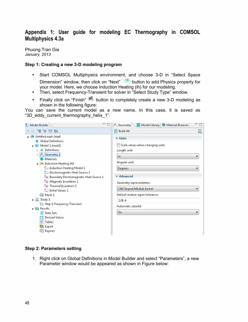
http://www.amazon.com/s/ref=ntt_athr_dp_sr_1?_encoding=UTF8&field-author=William%20H.%20Cubberly&search-alias=books&sort=relevancerank

48

Appendix 1: User guide for modeling EC Thermography in COMSOL Multiphysics 4.3a Phuong Tran Gia January, 2013

Step 1: Creating a new 3-D modeling program

• Start COMSOL Multiphysics environment, and choose 3-D in “Select Space

Dimension” window, then click on “Next” button to add Physics property for your model. Here, we choose Induction Heating (ih) for our modeling.

• Then, select Frequency-Transient for solver in “Select Study Type” window.

• Finally click on “Finish” button to completely create a new 3-D modeling as shown in the following figure:

You can save the current model as a new name. In this case, it is saved as “3D_eddy_current_thermography_helix_1”.

Step 2: Parameters setting

1. Right click on Global Definitions in Model Builder and select “Parameters”, a new Parameter window would be appeared as shown in Figure below:

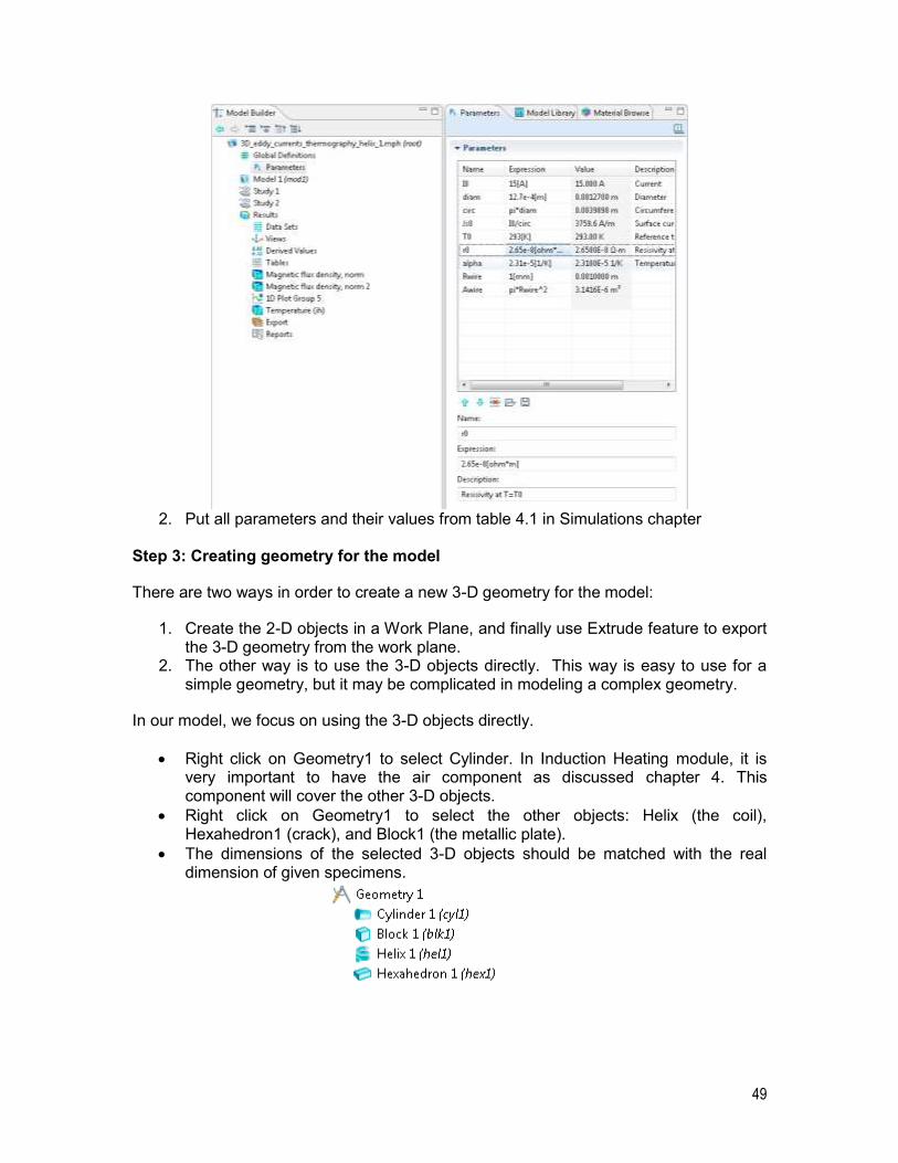
49

2. Put all parameters and their values from table 4.1 in Simulations chapter

Step 3: Creating geometry for the model

There are two ways in order to create a new 3-D geometry for the model:

1. Create the 2-D objects in a Work Plane, and finally use Extrude feature to export the 3-D geometry from the work plane.

2. The other way is to use the 3-D objects directly. This way is easy to use for a simple geometry, but it may be complicated in modeling a complex geometry.

In our model, we focus on using the 3-D objects directly.

Right click on Geometry1 to select Cylinder. In Induction Heating module, it is very important to have the air component as discussed chapter 4. This component will cover the other 3-D objects.

Right click on Geometry1 to select the other objects: Helix (the coil), Hexahedron1 (crack), and Block1 (the metallic plate).

The dimensions of the selected 3-D objects should be matched with the real dimension of given specimens.

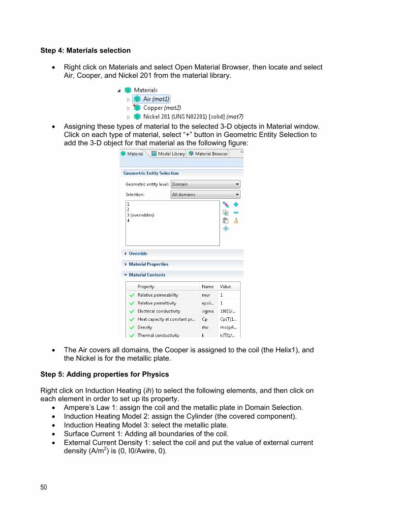
50

Step 4: Materials selection

Right click on Materials and select Open Material Browser, then locate and select Air, Cooper, and Nickel 201 from the material library.

Assigning these types of material to the selected 3-D objects in Material window.

Click on each type of material, select “+” button in Geometric Entity Selection to add the 3-D object for that material as the following figure:

The Air covers all domains, the Cooper is assigned to the coil (the Helix1), and the Nickel is for the metallic plate.

Step 5: Adding properties for Physics

Right click on Induction Heating (ih) to select the following elements, and then click on each element in order to set up its property.

Ampere’s Law 1: assign the coil and the metallic plate in Domain Selection.

Induction Heating Model 2: assign the Cylinder (the covered component).

Induction Heating Model 3: select the metallic plate.

Surface Current 1: Adding all boundaries of the coil.

External Current Density 1: select the coil and put the value of external current density (A/m2) is (0, I0/Awire, 0).

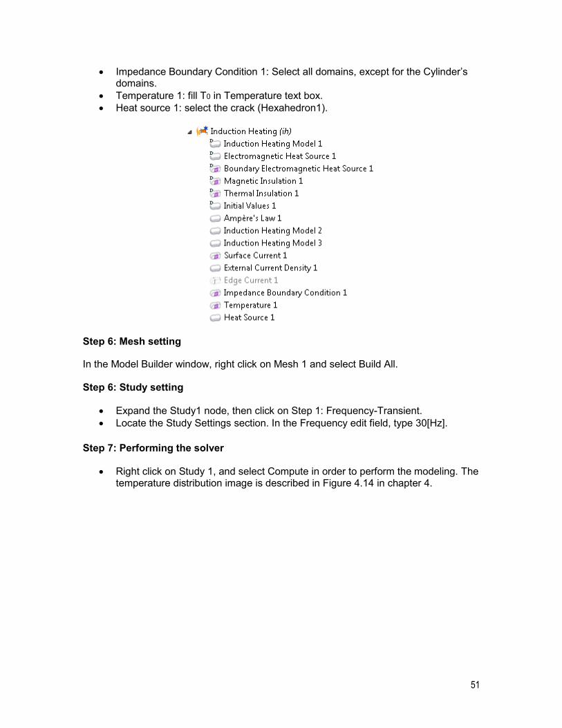
51

Impedance Boundary Condition 1: Select all domains, except for the Cylinder’s domains.

Temperature 1: fill T0 in Temperature text box.

Heat source 1: select the crack (Hexahedron1).

Step 6: Mesh setting

In the Model Builder window, right click on Mesh 1 and select Build All. Step 6: Study setting

Expand the Study1 node, then click on Step 1: Frequency-Transient.

Locate the Study Settings section. In the Frequency edit field, type 30[Hz].

Step 7: Performing the solver

Right click on Study 1, and select Compute in order to perform the modeling. The temperature distribution image is described in Figure 4.14 in chapter 4.

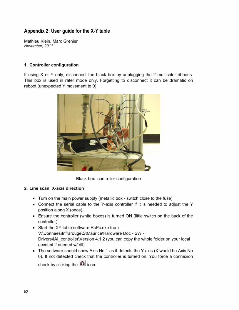
52

Appendix 2: User guide for the X-Y table

Mathieu Klein, Marc Grenier November, 2011

1. Controller configuration

If using X or Y only, disconnect the black box by unplugging the 2 multicolor ribbons.

This box is used in rater mode only. Forgetting to disconnect it can be dramatic on

reboot (unexpected Y movement to 0)

Black box- controller configuration

2. Line scan: X-axis direction

Turn on the main power supply (metallic box - switch close to the fuse)

Connect the serial cable to the Y-axis controller if it is needed to adjust the Y

position along X (once).

Ensure the controller (white boxes) is turned ON (little switch on the back of the

controller)

Start the XY table software RcPc.exe from

V:\Donnees\Infrarouge\StMaurice\Hardware Doc - SW -

Drivers\IAI_controller\Version 4.1.2 (you can copy the whole folder on your local

account if needed w/ dll)

The software should show Axis No 1 as it detects the Y axis (X would be Axis No

0). If not detected check that the controller is turned on. You force a connexion

check by clicking the icon.

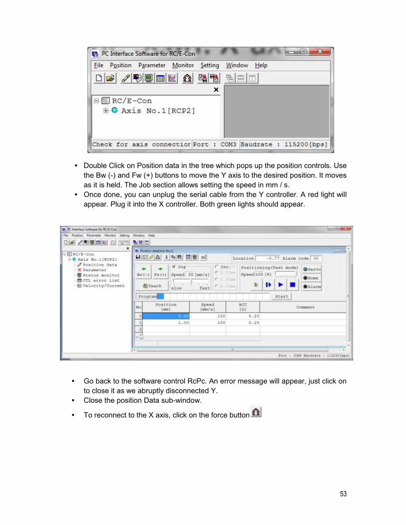
53

• Double Click on Position data in the tree which pops up the position controls. Use

the Bw (-) and Fw (+) buttons to move the Y axis to the desired position. It moves

as it is held. The Job section allows setting the speed in mm / s.

• Once done, you can unplug the serial cable from the Y controller. A red light will

appear. Plug it into the X controller. Both green lights should appear.

• Go back to the software control RcPc. An error message will appear, just click on

to close it as we abruptly disconnected Y.

• Close the position Data sub-window.

• To reconnect to the X axis, click on the force button

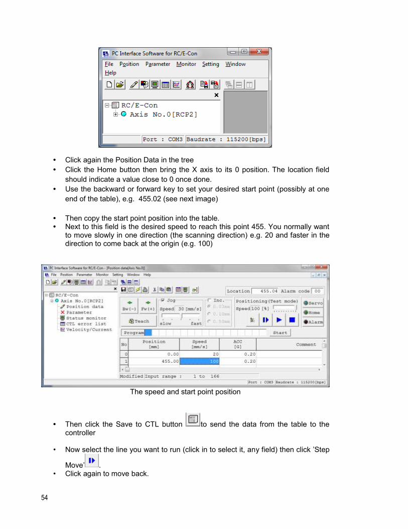
54

• Click again the Position Data in the tree

• Click the Home button then bring the X axis to its 0 position. The location field

should indicate a value close to 0 once done.

• Use the backward or forward key to set your desired start point (possibly at one

end of the table), e.g. 455.02 (see next image)

• Then copy the start point position into the table. • Next to this field is the desired speed to reach this point 455. You normally want

to move slowly in one direction (the scanning direction) e.g. 20 and faster in the direction to come back at the origin (e.g. 100)

The speed and start point position

• Then click the Save to CTL button to send the data from the table to the controller

• Now select the line you want to run (click in to select it, any field) then click ’Step

Move’ . • Click again to move back.

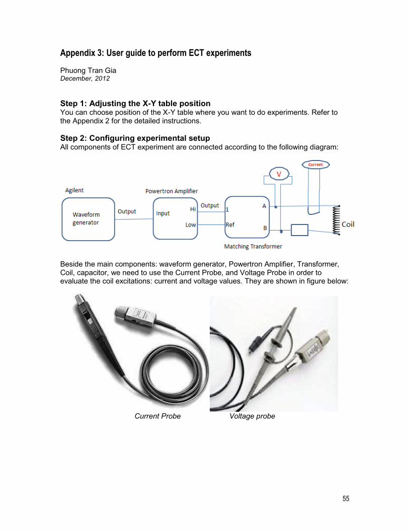
55

Appendix 3: User guide to perform ECT experiments

Phuong Tran Gia December, 2012

Step 1: Adjusting the X-Y table position You can choose position of the X-Y table where you want to do experiments. Refer to the Appendix 2 for the detailed instructions.

Step 2: Configuring experimental setup All components of ECT experiment are connected according to the following diagram:

Beside the main components: waveform generator, Powertron Amplifier, Transformer, Coil, capacitor, we need to use the Current Probe, and Voltage Probe in order to evaluate the coil excitations: current and voltage values. They are shown in figure below:

Current Probe Voltage probe

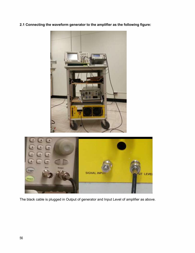
56

2.1 Connecting the waveform generator to the amplifier as the following figure:

The black cable is plugged in Output of generator and Input Level of amplifier as above.

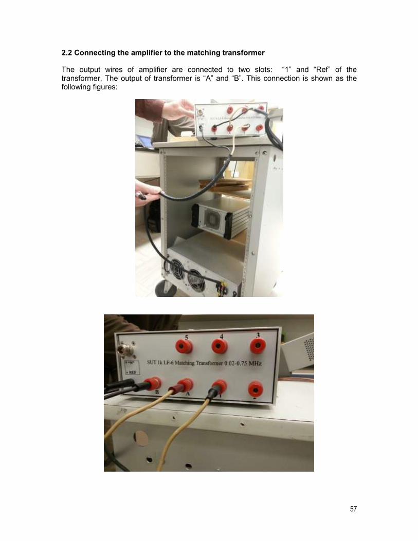
57

2.2 Connecting the amplifier to the matching transformer

The output wires of amplifier are connected to two slots: “1” and “Ref” of the transformer. The output of transformer is “A” and “B”. This connection is shown as the following figures:

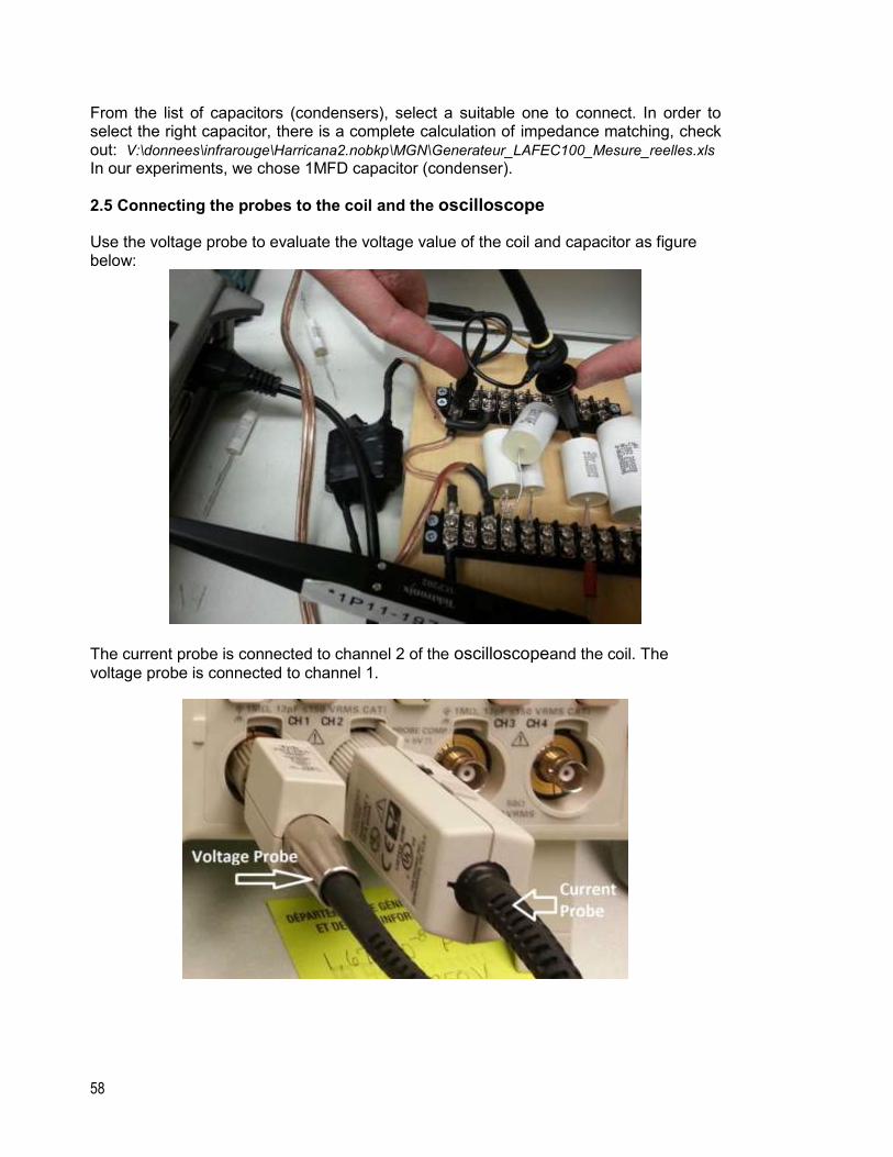
58

From the list of capacitors (condensers), select a suitable one to connect. In order to select the right capacitor, there is a complete calculation of impedance matching, check out: V:\donnees\infrarouge\Harricana2.nobkp\MGN\Generateur_LAFEC100_Mesure_reelles.xls

In our experiments, we chose 1MFD capacitor (condenser).

2.5 Connecting the probes to the coil and the oscilloscope

Use the voltage probe to evaluate the voltage value of the coil and capacitor as figure below:

The current probe is connected to channel 2 of the oscilloscopeand the coil. The

voltage probe is connected to channel 1.

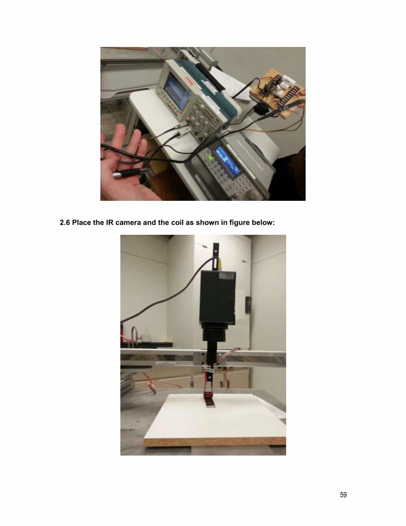
59

2.6 Place the IR camera and the coil as shown in figure below:

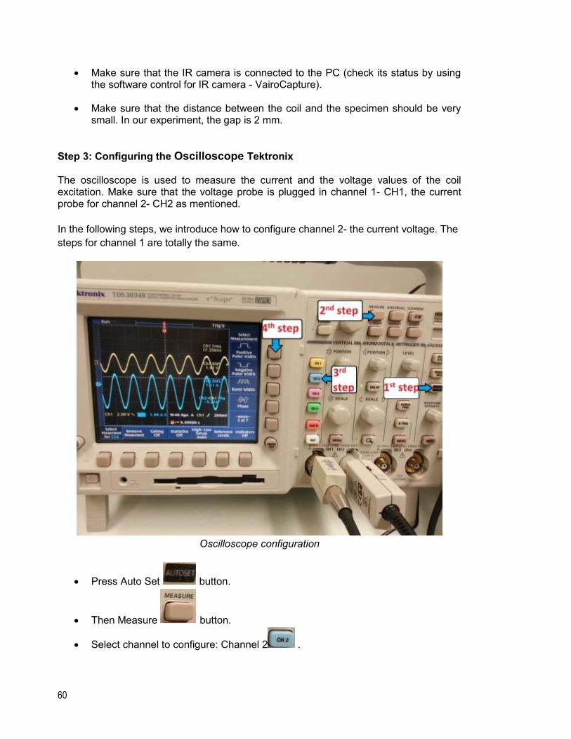
60

Make sure that the IR camera is connected to the PC (check its status by using the software control for IR camera - VairoCapture).

Make sure that the distance between the coil and the specimen should be very small. In our experiment, the gap is 2 mm.

Step 3: Configuring the Oscilloscope Tektronix

The oscilloscope is used to measure the current and the voltage values of the coil excitation. Make sure that the voltage probe is plugged in channel 1- CH1, the current probe for channel 2- CH2 as mentioned.

In the following steps, we introduce how to configure channel 2- the current voltage. The

steps for channel 1 are totally the same.

Oscilloscope configuration

Press Auto Set button.

Then Measure button.

Select channel to configure: Channel 2 .

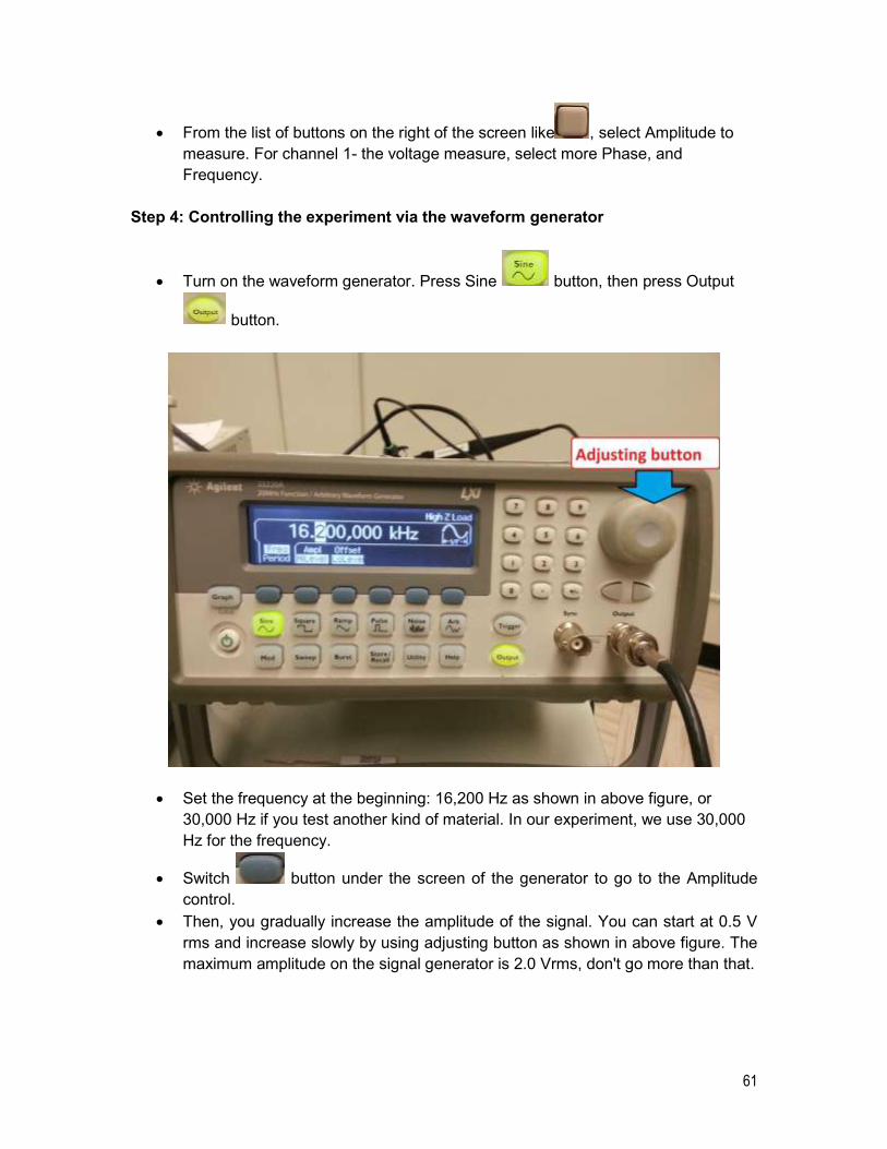
61

From the list of buttons on the right of the screen like , select Amplitude to

measure. For channel 1- the voltage measure, select more Phase, and

Frequency.

Step 4: Controlling the experiment via the waveform generator

Turn on the waveform generator. Press Sine button, then press Output

button.

Set the frequency at the beginning: 16,200 Hz as shown in above figure, or

30,000 Hz if you test another kind of material. In our experiment, we use 30,000

Hz for the frequency.

Switch button under the screen of the generator to go to the Amplitude

control.

Then, you gradually increase the amplitude of the signal. You can start at 0.5 V

rms and increase slowly by using adjusting button as shown in above figure. The

maximum amplitude on the signal generator is 2.0 Vrms, don't go more than that.

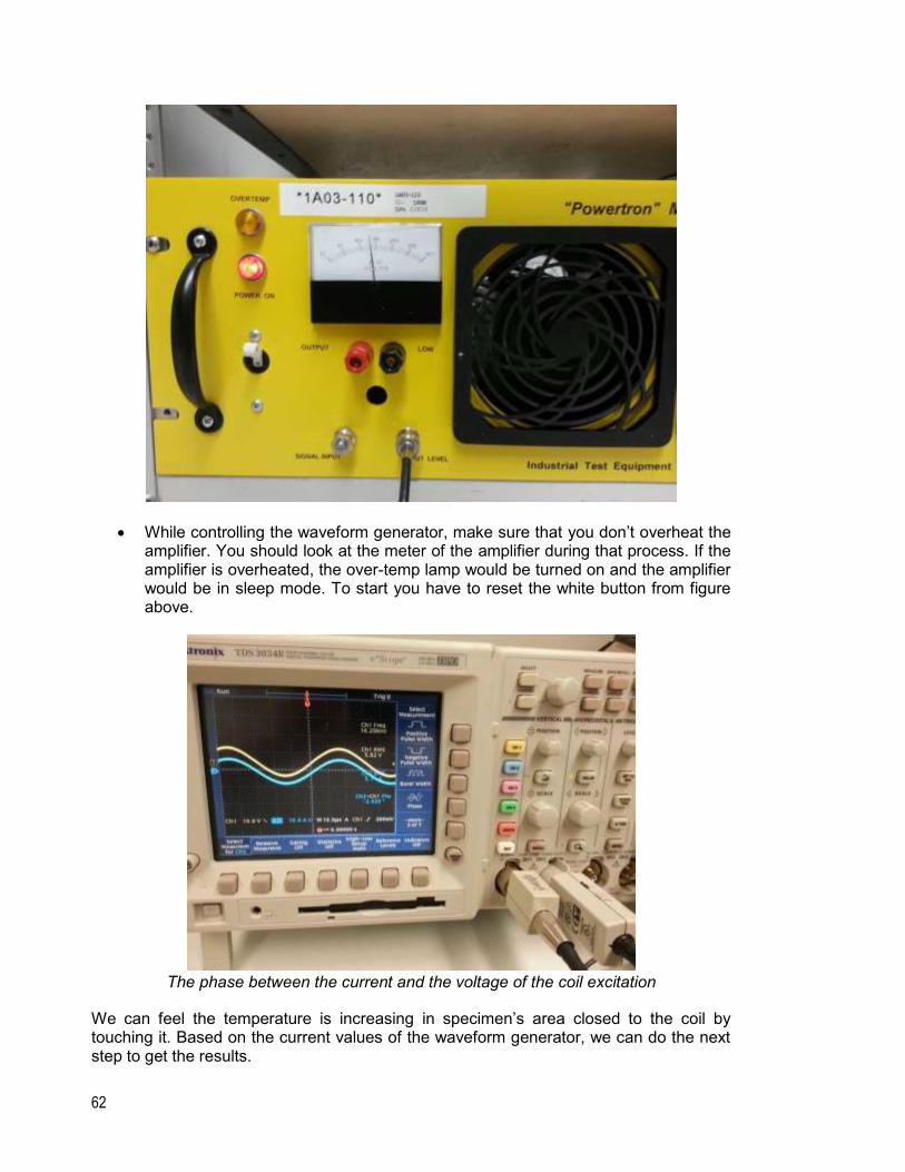
62

While controlling the waveform generator, make sure that you don’t overheat the amplifier. You should look at the meter of the amplifier during that process. If the amplifier is overheated, the over-temp lamp would be turned on and the amplifier would be in sleep mode. To start you have to reset the white button from figure above.

The phase between the current and the voltage of the coil excitation

We can feel the temperature is increasing in specimen’s area closed to the coil by touching it. Based on the current values of the waveform generator, we can do the next step to get the results.

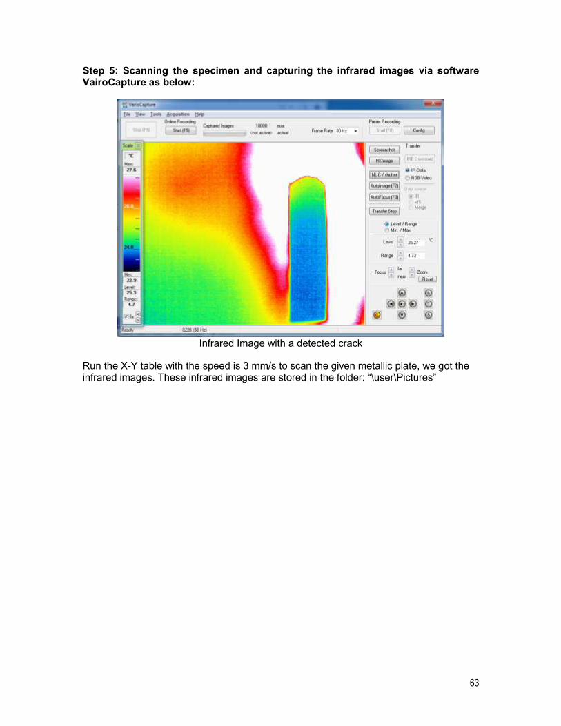
63

Step 5: Scanning the specimen and capturing the infrared images via software VairoCapture as below:

Infrared Image with a detected crack

Run the X-Y table with the speed is 3 mm/s to scan the given metallic plate, we got the infrared images. These infrared images are stored in the folder: “\user\Pictures”

Documents

Crack Inspection and simulations with Eddy Current ......Crack Inspection and simulations with Eddy Current Thermography for the Aerospace Industry Mémoire Gia Phuong Tran Maîtrise