HAL Id: hal-01764616https://hal.inria.fr/hal-01764616

Submitted on 12 Apr 2018

HAL is a multi-disciplinary open accessarchive for the deposit and dissemination of sci-entific research documents, whether they are pub-lished or not. The documents may come fromteaching and research institutions in France orabroad, or from public or private research centers.

L’archive ouverte pluridisciplinaire HAL, estdestinée au dépôt et à la diffusion de documentsscientifiques de niveau recherche, publiés ou non,émanant des établissements d’enseignement et derecherche français ou étrangers, des laboratoirespublics ou privés.

Coarse large-eddy simulations in a transitional wake flowwith flow models under location uncertainty

Pranav Chandramouli, Dominique Heitz, Sylvain Laizet, Etienne Mémin

To cite this version:Pranav Chandramouli, Dominique Heitz, Sylvain Laizet, Etienne Mémin. Coarse large-eddy simula-tions in a transitional wake flow with flow models under location uncertainty. Computers and Fluids,Elsevier, 2018, 168, pp.170-189. 10.1016/j.compfluid.2018.04.001. hal-01764616

Coarse large-eddy simulations in a transitional wake

flow with flow models under location uncertainty

Pranav Chandramoulia,∗, Dominique Heitzb, Sylvain Laizetc, EtienneMemina

aINRIA, Fluminance group, Campus universitaire de Beaulieu, F-35042 Rennes Cedex,France.

bIrstea, UR OPAALE, F-35044 Rennes Cedex, France.cDepartment of Aeronautics, Imperial College London, London, United Kingdom.

Abstract

The focus of this paper is to perform coarse-grid large eddy simulation (LES)using recently developed sub-grid scale (SGS) models of cylinder wake flowat Reynolds number (Re) of 3900. As we approach coarser resolutions, adrop in accuracy is noted for all LES models but more importantly, the nu-merical stability of classical models is called into question. The objective isto identify a statistically accurate, stable sub-grid scale (SGS) model for thistransitional flow at a coarse resolution. The proposed new models under loca-tion uncertainty (MULU) are applied in a deterministic coarse LES contextand the statistical results are compared with variants of the Smagorinskymodel and various reference data-sets (both experimental and Direct Nu-merical Simulation (DNS)). MULU are shown to better estimate statisticsfor coarse resolution (at 0.46% the cost of a DNS) while being numericallystable. The performance of the MULU is studied through statistical compar-isons, energy spectra, and sub-grid scale (SGS) contributions. The physicsbehind the MULU are characterised and explored using divergence and curlfunctions. The additional terms present (velocity bias) in the MULU areshown to improve model performance. The spanwise periodicity observed atlow Reynolds is achieved at this moderate Reynolds number through the curlfunction, in coherence with the birth of streamwise vortices.

Keywords:

∗Corresponding author.Email address: pranav.chandramouli@inria.fr (Pranav Chandramouli)

Preprint submitted to Computers & Fluids April 4, 2018

Large Eddy Simulation, Cylinder Wake Flow

1. Introduction

Cylinder wake flow has been studied extensively starting with the exper-imental works of Townsend (1; 2) to the numerical works of Kravchenko andothers (3; 4; 5). The flow exhibits a strong dependance on Reynolds numberRe = UD/ν, where U is the inflow velocity, D is the cylinder diameter andν is the kinematic viscosity of the fluid. Beyond a critical Reynolds numberRe ∼ 40 the wake becomes unstable leading to the well known von Karmanvortex street. The eddy formation remains laminar until gradually being re-placed by turbulent vortex shedding at higher Re. The shear layers remainlaminar until Re ∼ 400 beyond which the transition to turbulence takesplace up to Re = 105 - this regime, referred to as the sub-critical regime, isthe focus of this paper.

The transitional nature of the wake flow in the sub-critical regime, espe-cially in the shear layers is a challenging problem for turbulence modellingand hence has attracted a lot of attention. The fragile stability of the shearlayers leads to more or less delayed roll-up into von Karman vortices andshorter or longer vortex formation regions. As a consequence significant dis-crepancies have been observed in near wake quantities both for numericalsimulations (6) and experiments (7).

Within the sub-critical regime, 3900 has been established as a benchmarkRe. The study of (7) provides accurate experimental data-set showing goodagreement with previous numerical studies contrary to early experimentaldatasets (8). The early experiments of Lourenco and Shih (9) obtained aV-shaped mean streamwise velocity profile in the near wake contrary to theU-shaped profile obtained by (8). The discrepancy was attributed to inac-curacies in the experiment - a fact confirmed by the studies of (10) and (4).Parnaudeau et al.’s (7) experimental database, which obtains the U-shapedmean profile in the near wake, is thus becoming useful for numerical valida-tion studies. With increasing computation power, the LES data sets at Re= 3900 have been further augmented with DNS studies performed by (6).

The transitional nature of the flow combined with the availability of vali-dated experimental and numerical data-sets at Re = 3900 makes this an idealflow for model development and comparison. The LES model parametrisa-tion controls the turbulent dissipation. A good SGS model should ensure

2

suitable dissipation mechanism. Standard Smagorinsky model (11) basedon an equilibrium between turbulence production and dissipation, has a ten-dency to overestimate dissipation in general (12). In transitional flows, wherethe dissipation is weak, such a SGS model leads to laminar regimes, forexample, in the shear layers for cylinder wake. Different modifications ofthe model have been proposed to correct this behaviour. As addressed by(12), who introduced relevant improvements, the model coefficients exhibita strong dependency both on the ratio between the integral length scale andthe LES filter width, and on the ratio between the LES filter width and theKolmogorov scale. In this context of SGS models, coarse LES remains achallenging issue.

The motivation for coarse LES is dominated by the general interest to-wards reduced computational cost which could pave the way for performinghigher Re simulations, sensitivity analyses, and Data Assimilation (DA) stud-ies. DA has gathered a lot of focus recently with the works of (13), (14), and(15) but still remains limited by computational requirement.

With the focus on coarse resolution, this study analyses the performanceof LES models for transitional wake flow at Re 3900. The models underlocation uncertainty (16; 17) are analysed in depth for their performanceat a coarse resolution and compared with classical models. The models areso called as the equations are derived assuming that the location of a fluidparcel is known only up to a random noise i.e. location uncertainty. Withinthis reformulation of the Navier-Stokes equations, the contributions of thesubgrid scale random component is split into an inhomogeneous turbulentdiffusion and a velocity bias which corrects the advection due to resolvedvelocity field. Such a scheme has been shown to perform well on the TaylorGreen vortex flow (18) at Reynolds number of 1600, 3000, and 5000. The newscheme was shown to outperform the established dynamic Smagorinky modelespecially at higher Re. However, this flow is associated to an almost isotropicturbulence and no comparison with data is possible (as it is a pure numericalflow). Here we wish to assess the model skills with respect to more complexsituations (with laminar, transient and turbulent areas) and coarse resolutiongrids. We provide also a physical analysis of the solutions computed andcompare them with classical LES schemes and experimental data. Althoughthe models are applied to a specific Reynolds number, the nature of theflow generalises the applicability of the results to a wide range of Reynoldsnumber from 103− 105, i.e. up to the pivotal point where the transition intoturbulence of the boundary layer starts at the wall of the cylinder. The goal

3

is to show the ability of such new LES approaches for simulation at coarseresolution of a wake flow in the subcritical regime. Note that recently forthe same flow configuration, (19) have derived the MULU in a reduced-orderform using Proper Orthogonal Decomposition (POD), successfully providingphysical interpretations of the local corrective advection and diffusion terms.The authors showed that the near wake regions like the pivotal zone of theshear layers rolling into vortices are key players into the modelling of theaction of small-scale unresolved flow on the resolved flow .

In the following, we will show that the MULU are able to capture, in thecontext of coarse simulation, the essential physical mechanisms of the tran-sitional very near wake flow. This is due to the split of the SGS contributioninto directional dissipation and velocity bias. The next section elaborates onthe various SGS models analysed in this study followed by a section on theflow configuration and numerical methods used. A comparison of the elab-orated models and the associated physics is provided in the results section.Finally, a section of concluding remarks follows.

2. Models under location uncertainty

General classical models such as Smagorinsky or Wall-Adaptive LocalEddy (WALE) viscosity model proceed through a deterministic approachtowards modelling the SGS dissipation tensor. However, (16) suggests astochastic approach towards modelling the SGS contributions in the Navier-Stokes (NS) equation. Building a stochastic NS formulation can be achievedvia various methods. The simplest way consists in considering an additionaladditive random forcing (20). Other modelling considered the introductionof fluctuations in the subgrid models (21; 22). Also, in the wake of Kraich-nan’s work (23) another choice consisted in closing the large-scale flow inthe Fourier space from a Langevin equation (24; 25; 26). Lagrangian modelsbased on Langevin equation in the physical space have been also successfullyproposed for turbulent dispersion (27) or for probability density function(PDF) modelling of turbulent flows (28; 29; 30). These attractive modelsfor particle based representation of turbulent flows are nevertheless not wellsuited to a large-scale Eulerian modelling.

In this work we rely on a different stochastic framework of the NS equationrecently derived from the splitting of the Lagrangian velocity into a smoothcomponent and a highly oscillating random velocity component (i.e. the

4

uncertainty in the parcel location expressed as velocity) (16):

dXt

dt= u(Xt, t) + σ(Xt, t)B

The first term, on the right-hand side represents the large-scale smooth veloc-ity component, while the second term is the small-scale component. This lat-ter term is a random field defined from a Brownian term function B = dB/dtand a diffusion tensor σ. The small-scale component is rapidly decorrelatingat the resolved time scale with spatial correlations (which might be inhomoge-neous and non stationary) fixed through the diffusion tensor. It is associatedwith a covariance tensor:

Qij(x,y, t, t′) = E((σ(x, t)dBt)(σ(x, t)dBt)

T ) = cij(x,y, t)δ(t− t′)dt. (1)

In the following the diagonal of the covariance tensor, termed here as the

variance tensor, plays a central role; it is denoted as a(x)4= c(x, t). This

tensor is a (3 × 3) symmetric positive definite matrix with dimension of aviscosity in m2 s−1.

With such a decomposition, the rate of change of a scalar within a ma-terial volume, is given through a stochastic representation of the ReynoldsTransport Theorem (RTT) (16; 17). For an incompressible small-scale ran-dom component (∇·σ = 0) the RTT has the following expression:

d

∫V(t)

q =

∫V(t)

(dtq+

(∇·(qu)− 1

2

d∑i,j=1

∂xi(aij∂xjq))dt+∇q ·σdBt

)dx. (2)

where the effective advection u is defined as:

u = u− 1

2∇ · a. (3)

The first term on the right-hand side represents the variation of quantityq with respect to time: dtq = q(x, t+dt)−q(x, t). It is similar to the temporalderivative. It is important here to quote that q is a non differentiable randomfunction that depends among other things on the particles driven by theBrownian component and flowing through a given location. The secondterm on the right-hand side stands for the scalar transport by the large-scale velocity. However, it can be noticed that this scalar advection is not

5

purely a function of the large-scale velocity. Indeed, the large-scale velocityis here affected by the inhomogeneity of the small-scale component througha modified large-scale advection (henceforth termed as velocity bias u ),where the effect of the fluctuating component is taken into account via thesmall-scale velocity auto-correlations a = (σσT ). A similar modification ofthe large-scale velocity was also suggested in random walks Langevin modelsby (31) who studied various stochastic models for particle dispersion - theyconcluded that an artificially introduced bias velocity to counter particle driftwas necessary to optimise the models for a given flow. In the framework ofmodelling under location uncertainty, this term appears automatically. Thethird term in the stochastic RTT corresponds to a diffusion contributiondue to the small-scale components. This can be compared with the SGSdissipation term in LES Modelling. This dissipation term corresponds toa generalization of the classical SGS dissipation term, which ensues in theusual context from the Reynolds decomposition and the Boussinesq’s eddyviscosity assumption. Here it figures the mixing effect exerted by the small-scale component on the large-scale component. Despite originating froma very different construction, in the following, for ease of reference, we keepdesignating this term as the SGS contribution. The final term in the equationis the direct scalar advection by the small-scale noise.

It should be noted that the RTT corresponds to the differential of thecomposition of two stochastic processes. The Ito formulae, which is restrictedto deterministic functions of a stochastic process, does not apply here. Anextended formulae know as Ito-Wentzell (or generalized Ito) formulae mustbe used instead (32).

Using the Stochastic RTT, the large-scale flow conservation equationscan be derived (for the full derivation please refer to (16; 17)). The finalconservation equations are presented below:

Mass conservation:

dtρ+∇ · (ρu)dt+∇ρ ·σ dBt =1

2∇ · (a∇ρ)dt, (4)

which simplifies to the following constraints for an incompressible fluid:

∇ · σ = 0, ∇ · u = 0, (5)

The first constraint maintains a divergence free small-scale velocity field,while the second imposes the same for the large smooth effective component.

6

We observe that the large-scale component, u, is allowed to be diverging,with a divergence given by ∇ ·∇ · a. As we shall see, this value is in prac-tice quite low. This weak incompressibility constraint results in a modifiedpressure computation, which is numerically not difficult to handle. Imposinginstead a stronger incompressibility constraint on u introduces an additionalcumbersome constraint on the variance tensor (∇ ·∇ · a = 0). In this workwe will rely on the weak form of the incompressibility constraint. The large-scale momentum equation boils down to a large-scale deterministic equationafter separation between the bounded variation terms (i.e. terms in ”dt”)and the Brownian terms, which is rigorously authorized - due to uniquenessof this decomposition.

Momentum conservation:(∂tu + u∇T (u− 1

2∇ · a)− 1

2

∑ij

∂xi(aij∂xju)

)ρ = ρg −∇p+ µ∆u. (6)

Similar to the deterministic version of the NS equation, we have the flowmaterial derivative, the forces, and viscous dissipation. The difference liesin the modification of the advection which includes the velocity bias and thepresence of the dissipation term which can be compared with the SGS termpresent in the filtered NS equation. Both the additional terms present inthe stochastic version are computed via the auto-correlation tensor a. Thusto perform a LES, one needs to model, either directly or through the small-scale noise, the auto-correlation tensor. Two methodologies can be envisagedtowards this: the first would be to model the stochastic small-scale noise(σ(Xt, t)B) and thus evaluate the auto-correlation tensor. We term such anapproach as purely ‘stochastic LES’. The second method would be to modelthe auto-correlation tensor directly as it encompasses the total contributionof the small scales. This method can be viewed as a form of ‘deterministicLES’ using stochastically derived conservation equations and this is the ap-proach followed in this paper. The crux of the ‘deterministic LES’ approachthus revolves around the characterisation of the auto-correlation tensor. Thesmall-scale noise is considered subsumed within the mesh and is not definedexplicitly.

This opens up various possibilities for turbulence modelling. The spec-ification of the variance tensor a can be performed through an empiricallocal velocity fluctuation variance times a decorrelation time, or by physicalmodels/approximations or using experimental measurements. The options

7

explored in this study include physical approximation based models andempirical local variance based models as described below. Note that thisderivation can be applied to any flow model. For instance, such a modellinghas been successfully applied to derive stochastic large-scale representationof geophysical flows by (17; 33; 34).

A similar stochastic framework arising also from a decomposition of theLagrangian velocity has been proposed in (35) and analysed in (36) and (37).This framework leads to enstrophy conservation whereas the formulation un-der location uncertainty conserves the kinetic energy of a transported scalar(17).

2.0.1. Physical approximation based models:

Smagorinsky’s work on atmospheric flows and the corresponding modeldevelopement is considered to be the pioneering work on LES modelling (11).Based on Boussinesq’s eddy viscosity hypothesis which postulates that themomentum transfer caused by turbulent eddies can be modelled by an eddyviscosity (νt) combined with Prandtl’s mixing length hypothesis he developeda model (Smag) for characterising the SGS dissipation.

νt = C||S||, (7)

τ = C||S||S, (8)

where τ stands for the SGS stress tensor, C is the Smagorinsky coefficientdefined as (Cs∆)2, where ∆ is the LES filter width, ||S|| = 1

2[∑

ij(∂xiuj +

∂xjui)2]

12 is the Frobenius norm of the rate of strain tensor, and

Sij =1

2(∂ui∂xj

+∂uj∂xi

). (9)

Similar to Smagorinsky’s eddy viscosity model, the variance tensor forthe formulation under location uncertainty can also be specified using thestrain rate tensor. Termed in the following as the Stochastic Smagorinskymodel (StSm), it specifies the variance tensor similar to the eddy viscosityin the Classical Smagorinsky model:

a(x, t) = C||S||I3, (10)

where I3 stands for 3× 3 identity matrix and C is the Smagorinsky coefficient.The equivalency between the two models can be obtained in the followingcase (as shown by (16)):

8

The SGS contribution (effective advection and SGS dissipation) for theStSm model is:

uj∂xj(∂xjakj) +∑ij

∂xi(aij∂xjuk) = uj∂xj(∂xj ||S||δkj) +∑ij

∂xi(||S||δij∂xjuk),

= uk∆||S||+ ||S||∆uk +∑j

∂xj ||S||∂xjuk,

(11)

and the SGS contribution for Smagorinsky model (∇ · τ ) is:

∇ · τ =∑j

∂xj(||S||S),

=∑j

∂xj(||S||(∂xjuk + ∂xkuj)),

=∑j

∂xj ||S||∂xjuk + ∂xj ||S||∂xkuj + ||S||∆uk.

(12)

An equivalency can be drawn between the two models by adding∑

j ∂xj ||S||∂xkuj−uk∆||S|| to the StSm model. The additional term may also be written as:

∂xk∑j

∂xj(||S||)uj −∑j

∂xj∂xk(||S||)uj − uk∆||S||, (13)

where the first term represents a velocity gradient which can be includedwithin a modified pressure term as is employed for Smagorinsky model. Theother two terms can be neglected for smooth enough strain rate tensor func-tion. For smooth deformations both models are equivalent in terms of dis-sipation. It is important to note here that even if the effective advection isignored in the StSm model, the two models still differ in a general case dueto the first two terms in (13).

Smagorinsky’s pioneering work remains to date a popular model for LES,however it has certain associated drawbacks. The model assumes the exis-tence of equilibrium between the kinetic energy flux across scale and the largescales of turbulence - this equilibrium is not established in many cases suchas the leading edge of an airplane wing or turbulence with strong buoyancy.In addition, a form of arbitrariness and user dependency is introduced dueto the presence of the Smagorinsky coefficient. This coefficient is assumed tobe constant irrespective of position and time. Lilly (38) suggests a constant

9

coefficient value to be appropriate for the Smagorinsky model. However thiswas disproved by the works of (12), and (39) who shows that a constant valuedid not efficiently capture turbulence especially in boundary layers.

Numerous attempts were made to correct for the fixed constant such asdamping functions (40) or renormalisation group theory (41). Germano et al.(39) provided a non ad-hoc manner of calculating the Smagorinsky coefficientvarying with space and time using the Germano identity and an additionaltest filter t (termed as the Dynamic Smagorinsky (DSmag) model).

Lij = Tij − τ tij, (14)

where τ stands for the SGS stress filtered by the test filter t, T is the filteredSGS stress calculated from the test filtered velocity field, and L stands for theresolved turbulent stress. The Smagorinsky coefficient can thus be calculatedas:

C2s =

< LijMij >

< MijMij >,where (15)

Mij = −2∆2(α′2||St||Stij − (||S||Sij)t (16)

and α′

stands for the ratio between the test filter and the LES filter.The dynamical update procedure removes the user dependancy aspect

in the model, however it introduces unphysical values for the coefficient atcertain instances. An averaging procedure along a homogenous direction isnecessary to provide physical values for Cs. However, most turbulent flows,foremost being wake flow around a cylinder, lack a homogenous direction foraveraging. In such cases, defining the coefficient is difficult and needs ad-hoc measures such as local averaging, threshold limitation, and/or filteringmethods to provide nominal values for Cs. For the present study, we focuson the classical and dynamic variations of the Smagorinsky model - thesemodel were used to study cylinder wake flow by (8), (42), (43), among manyothers.

2.0.2. Local variance based models:

As the name states, the variance tensor can be calculated by an empiricalcovariance of the resolved velocity within a specified local neighbourhood.The neighbourhood can be spatially or temporally located giving rise totwo formulations. A spatial neighbourhood based calculation (referred to as

10

Stochastic Spatial Variance model (StSp)) is given as:

a(x, nδt) =1

|Γ| − 1

∑xi∈η(x)

(u(xi, nδt)− u(x, nδt))(u(xi, nδt)− u(x, nδt))TCsp,

(17)where u(x, nδt) stands for the empirical mean around the arbitrarily selectedlocal neighbourhood defined by Γ. The constant Csp is defined as (18):

Csp =

(`resη

) 53

∆t, (18)

where `res is the resolved length scale, η is the Kolmogorov length scale and∆t is the simulation time step.

A similar local variance based model can be envisaged in the temporalframework; however, it has not been analysed in this paper due to memorylimitations.

It is important to note that the prefix stochastic has been added to theMULU to differentiate the MULU version of the Smagorinsky model fromits classical purely deterministic version. The model equations while derivedusing stochastic principles are applied in this work in a purely deterministicsense. The full stochastic formulation of MULU has been studied by (17).

3. Flow configuration and numerical methods

The flow was simulated using a parallelised flow solver, Incompact3d, de-veloped by (44). Incompact3d relies on a sixth order finite difference scheme(the discrete schemes are described in (45)) and the Immersed BoundaryMethod (IBM) (for more details on IBM refer to (46)) to emulate a bodyforcing. The main advantage of using IBM is the ability to represent themesh in cartesian coordinates and the straightforward implementation ofhigh-order finite difference schemes in this coordinate system. The IBM inIncompact3d has been applied effectively to cylinder wake flow by (7) andto other flows by (46), and (47) among others. A detailed explanation ofthe IBM as applied in Incompact3d, as well as its application to cylinderwake flow can also be found in (7). It is important to note that this paperfocuses on the accuracy of the sub-grid models within the code and not onthe numerical methodology (IBM/numerical schemes) of the code itself.

The incompressibility condition is treated with a fractional step methodbased on the resolution of a Poisson equation in spectral space on a staggered

11

pressure grid combined with IBM. While solving the Poisson equation for thestochastic formulation, the velocity bias was taken into account in order tosatisfy the stochastic mass conservation constraints. It can be noted thatalthough the solution of the Poisson equation in physical space is computa-tionally heavy, the same when performed in Fourier space is cheap and easilyimplemented with Fast Fourier transforms. For more details on Incompact3dthe authors refer you to (44) and (48).

The flow over the cylinder is simulated for a Re of 3900 on a domain mea-suring 20D × 20D × πD. The cylinder is placed in the centre of the lateraldomain at 10D and at 5D from the domain inlet. For statistical purposes,the centre of the cylinder is assumed to be (0, 0). A coarse mesh resolutionof 241 × 241 × 48 is used for the coarse LES (cLES). cLES discretisationhas been termed as coarse as this resolution is ∼ 6.2% the resolution of thereference LES of (7) (henceforth referred to as LES - Parn). In terms ofKolmogorov units (η), the mesh size for the cLES is 41η × 7η - 60η × 32η.The Kolmogorov length scale has been calculated based on the dissipationrate and viscosity, where the dissipation rate can be estimated as ε ∼ U3/Lwhere U and L are the characteristic velocity scale and the integral lengthscale. A size range for y is used due to mesh stretching along the lateral (y)direction which provides a finer mesh in the middle. Despite the stretching,the minimum mesh size for the cLES is still larger than the mesh size of par-ticle imagery velocimetry (PIV) reference measurements of (7) (henceforthreferred to as PIV - Parn). For all simulations, inflow/outflow boundarycondition is implemented along the streamwise (x) direction with free-slipand periodic boundary conditions along the lateral (y) and spanwise (z) di-rections respectively - the size of the spanwise domain has been fixed to πDas set by (8), which was also validated by (7) to be sufficient with periodicboundary conditions. The turbulence is initiated in the flow by introducinga white noise in the initial condition. Time advancement is performed usingthe third order Adam-Bashforth scheme. A fixed coefficient of 0.1 is usedfor the Smagorinsky models as suggested in literature (43) while a spatialneighbourhood of 7 × 7 × 7 is used for the Stochastic Spatial model. Forthe dynamic Smagorinsky model, despite the lack of clear homogenous direc-tion, a spanwise averaging is employed. In addition, the constant is filteredand a threshold on negative and large positive coefficients is also applied tostabilise the model. Note that the positive threshold is mesh dependant andneeds user-intervention to specify the limits.

The reference PIV (7) was performed with a cylinder of diameter 12 mm

12

and 280 mm in length placed 3.5D from the entrance of the testing zone in awind tunnel of length 100 cm and height 28 cm. Thin rectangular end platesplaced 240 mm apart were used with a clearance of 20 mm between the platesand the wall. 2D2C measurements were carried out at a free stream velocityof 4.6 m s−1 (Re ∼ 3900) recording 5000 image pairs separated by 25 µs witha final interrogation window measuring 16 × 16 pixels with relatively weaknoise. For more details about the experiment refer to (7).

The high resolution LES of (7) was performed on Incompact3d on thesame domain measuring 20D × 20D × πD with 961 × 961 × 48 cartesianmesh points. The simulation was performed with the structure functionmodel of (49) with a constant mesh size. LES - Parn is well resolved, how-ever, there is a distinct statistical mismatch between LES - Parn and PIV-Parn especially along the centre-line (see figure 1a and figure 1b). Litera-ture suggests that the wake behind the cylinder at a Re ∼ 3900 is highlyvolatile and different studies predict slightly varied profiles for the stream-wise velocity along the centre-line. The averaging time period, the type ofmodel, and the mesh type all affect the centre-line velocity profile. As canbe seen in figure 1a and figure 1b, each reference data set predicts a differ-ent profile/magnitude for the streamwise velocity profiles. The DNS studyof (6) does not present the centreline velocity profiles. This provided themotivation for performing a DNS study at Re ∼ 3900 to accurately quan-tify the velocity profiles and to reduce the mismatch between the existingexperimental and simulation datasets. The DNS was performed on the samedomain with 1537×1025×96 cartesian mesh points using Incompact3d withstretching implemented in the lateral (y) direction.

From figure 1a we can see that the DNS and the PIV of Parnaudeau arethe closest match among the data sets while significant deviation is seen inthe other statistics. In the fluctuating streamwise velocity profiles, the onlyother data sets that exist are of (50) who performed Laser Doppler Velocime-try (LDV) experiments at Re = 3000 and Re = 5000. Among the remain-ing data-sets (LES of Parnaudeau, PIV of Parnaudeau, and current DNS)matching profiles are observed for the DNS and PIV despite a magnitudedifference. These curves also match the profiles obtained by the experimentsof Norberg (50) in shape, i.e. the similar magnitude, dual peak nature. TheLES of Parnaudeau (7) is the only data-set to estimate an inflection point andhence is not considered further as a reference. The lower energy profile of thePIV may be attributed to the methods used for calculating the vector fieldswhich employ a large-scale representation of the flow via interrogation win-

13

Table 1: Flow parameters.

Re nx × ny × nz lx/D × ly/D × lz/D ∆x/D ∆y/D ∆z/D U∆t/D

cLES 3900 241×241×48 20×20×π 0.083 0.024-0.289 0.065 0.003DNS 3900 1537×1025×96 20×20×π 0.013 0.0056-0.068 0.033 0.00075

PIV - Parn 3900 160×128×1 3.6×2.9×0.083 0.023 0.023 0.083 0.01LES - Parn 3900 961×961×48 20×20×π 0.021 0.021 0.065 0.003

dows similar to a LES resolution (51). The DNS, however, exhibits a profilesimilar to other references and a magnitude in between the two LDV exper-iments of Norberg. Considering the intermediate Reynolds number of theDNS compared to the Norberg experiments, this suggests good convergenceand accuracy of the DNS statistics. Note that the cLES mesh is ∼ 0.46%the cost of the DNS. Table 1 concisely depicts all the important parametersfor the flow configuration as well as the reference datasets.

Wake flow around a cylinder was simulated in the above enumerated con-figuration with the following SGS models: Classic Smagorinsky (Smag), Dy-namic Smagorinsky (DSmag), Stochastic Smagorinsky (StSm), and Stochas-tic Spatial (StSp) variance. In accordance with the statistical compari-son performed by (8), first and second order temporal statistics have beencompared at 3 locations (x = 1.06D (top), x = 1.54D(middle), and x =2.02D(bottom)) in the wake of the cylinder. All cLES statistics are computed(after an initial convergence period) over 90,000 time steps corresponding to270 non-dimensional time or ∼ 54 vortex shedding cycles. All statistics arealso averaged along the spanwise (z) direction. The model statistics are eval-uated against the PIV experimental data of (7) and the DNS for which thedata has been averaged over 400,000 time steps corresponding to 60 vortexsheddings. The work of (7) suggests that at least 52 vortex sheddings areneeded for convergence which is satisfied for all the simulations. In addition,spanwise averaging of the statistics results in converged statistics compara-ble with the PIV ones. Both DNS and PIV statistics are provided for allstatistical comparison, however, the DNS is used as the principal referencewhen an ambiguity exists between the two references.

4. Results

In this section, we present the model results, performance analysis andphysical interpretations. Firstly, The cLES results are compared with the

14

−0.6

−0.4

−0.2

0

0.2

0.4

0.6

0.8

0.5 1 1.5 2 2.5 3 3.5 4 4.5

<u>

Uc

x/D

DNSPIV

LES-Parn

HWAL&S(1994)

O&W(1996)

K&M (2000)N:Re-3000 (1998)N:Re-5000 (1998)

(a)

0

0.02

0.04

0.06

0.08

0.1

0.12

0.14

0.5 1 1.5 2 2.5 3 3.5 4 4.5

<u′ u′ >

U2 c

x/D

DNSPIV

LES - ParnHWA

N: Re-3000N: Re-5000

(b)

Figure 1: Mean streamwise velocity (a) and fluctuating streamwise velocity (b) in thestreamwise direction along the centreline (y = 0) behind the cylinder for the referencedata-sets. Legend: HWA - hot wire anemometry(7), K&M - B-spline simulations (case II)of Kravchenko and Moin(4), L&S - experiment of Lourenco and Shih (9), N - experimentof Norberg at Re = 3000 and 5000 (50), O&W - experiement of Ong and Wallace (52)

reference PIV and the DNS. The focus on centreline results for certain com-parisons is to avoid redundancy and because these curves show maximumstatistical deviation. This is followed by a characterisation and physical anal-ysis of the velocity bias and SGS contributions for the MULU. The sectionis concluded with the computation costs of the different models.

4.1. Coarse LES

For cLES, the MULU have been compared with classic and dynamic ver-sion of the Smagorinksy model, DNS, and PIV - Parn. Figure 2 and figure3 depict the mean streamwise and lateral velocity respectively plotted alongthe lateral (y) direction. In the mean streamwise velocity profile (see figure2a), the velocity deficit behind the cylinder depicted via the U-shaped profilein the mean streamwise velocity is captured by all models. The expecteddownstream transition from U-shaped to a V-shaped profile is see for all themodels - a delay in transition is observed for Smag model which biases thestatistics at x = 1.54D and 2.02D. For the mean lateral component (see fig-ure 3), all models display the anti-symmetric quality with respect to y = 0.Smag model shows maximum deviation from the reference DNS statisticsin all observed profiles. All models but Smag capture the profile well whilebroadly StSp and DSmag models better capture the magnitude. As a generaltrend, Smag model can be seen to under-predict statistics while StSm model

15

over-predicts.

−0.2

0

0.2

0.4

0.6

0.8

1

1.2

1.4

1.6

−1 −0.5 0 0.5 1

<u>

Uc

y/D

(a) x/D = 1.06

−0.4

−0.2

0

0.2

0.4

0.6

0.8

1

1.2

1.4

−1 −0.5 0 0.5 1

<u>

Uc

y/D

(b) x/D = 1.54

−0.4

−0.2

0

0.2

0.4

0.6

0.8

1

1.2

−1 −0.5 0 0.5 1

<u>

Uc

y/D

(c) x/D = 2.02

PIV

DNS

Smag

StSm

DSmag

StSp

Figure 2: Mean streamwise velocity at 1.06D (top), 1.54D (middle), and 2.02D (bottom)in the wake of the circular cylinder.

A better understanding of the model performance can be obtained throughFigure 4 - 6 which depict the second order statistics, i.e. the rms componentof the streamwise (< u′u′ >) and lateral (< v′v′ >) velocity fluctuations andthe cross-component (< u′v′ >) fluctuations. The transitional state of theshear layer can be seen in the reference statistics by the two strong peaks atx = 1.06D in figure 4a. The magnitude of these peaks is in general under-predicted, however, a best estimate is given the MULU. DSmag and Smagmodels can be seen to under-predict these peaks at all x/D. This peak iseclipsed by a stronger peak further downstream due to the formation of theprimary vortices (see figure 4b) which is captured by all the models.

The maxima at the centreline for figure 5 and the anti-symmetric struc-ture for figure 6 are seen for all models. Significant mismatch is observed

16

−0.15

−0.1

−0.05

0

0.05

0.1

0.15

−1.5 −1 −0.5 0 0.5 1 1.5

<v>

Uc

y/D

(a) x/D = 1.06

−0.4

−0.3

−0.2

−0.1

0

0.1

0.2

0.3

0.4

−1.5 −1 −0.5 0 0.5 1 1.5

<v>

Uc

y/D

(b) x/D = 1.54

−0.3

−0.2

−0.1

0

0.1

0.2

0.3

−1.5 −1 −0.5 0 0.5 1 1.5

<v>

Uc

y/D

(c) x/D = 2.02

PIV

DNS

Smag

StSm

DSmag

StSp

Figure 3: Mean lateral velocity at 1.06D, 1.54D, and 2.02D in the wake of the circularcylinder.

between the reference and the Smag/StSm models especially in figure 5a and6a. In all second-order statistics, StSm model improves in estimation as wemove further downstream. No such trend is seen for StSp or DSmag mod-els while a constant under-prediction is seen for all Smag model statistics.This under-prediction could be due to the inherent over-dissipativeness ofthe Smagorinsky model which smooths the velocity field. This is correctedby DSmag/StSm models and in some instances over-corrected by the StSmmodel. A more detailed analysis of the two formulations under location un-certainty (StSm and StSp) is presented in sections 4.2.

The smoothing for each model is better observed in the 3D isocontours ofvorticity modulus (Ω) plotted in figure 7. Plotted at non-dimensional Ω = 7,the isocontours provide an understanding of the dominant vortex structureswithin the flow. While large-scale vortex structures are observed in all flows,

17

0

0.05

0.1

0.15

0.2

0.25

−1.5 −1 −0.5 0 0.5 1 1.5

<u′ u′ >

U2 c

y/D

(a) x/D = 1.06

0

0.05

0.1

0.15

0.2

0.25

−1.5 −1 −0.5 0 0.5 1 1.5

<u′ u′ >

U2 c

y/D

(b) x/D = 1.54

0

0.05

0.1

0.15

0.2

0.25

−1.5 −1 −0.5 0 0.5 1 1.5

<u′ u′ >

U2 c

y/D

(c) x/D = 2.02

PIV

DNS

Smag

StSm

DSmag

StSp

Figure 4: Streamwise rms velocity (u′u′) fluctuations at 1.06D, 1.54D, and 2.02D in thewake of the circular cylinder.

the small-scale structures and their spatial extent seen in the DNS are betterrepresented by the MULU. The over-dissipativeness of the Smag model leadsto smoothed isocontours with reduced spatial extent. The large-scale vortexstructures behind the cylinder exhibit the spanwise periodicity observed byWilliamson (53) for cylinder wake flow at low Re ∼ 270. Inferred to be due tomode B instability by Williamson, this spanwise periodicity was associatedwith the formation of small-scale streamwise vortex pairs. It is interesting toobserve here the presence of similar periodicity at higher Re - this periodicitywill be further studied at a later stage in this paper.

A stable shear layer associated with higher dissipation is observed inSmag model with the shear layer instabilities beginning further downstreamthan the MULU. An accurate shear layer comparison can be done by cal-culating the recirculation length (Lr) behind the cylinder. Also called the

18

0

0.01

0.02

0.03

0.04

0.05

0.06

0.07

0.08

0.09

0.1

−1.5 −1 −0.5 0 0.5 1 1.5

<v′ v′ >

U2 c

y/D

(a) x/D = 1.06

0

0.05

0.1

0.15

0.2

0.25

0.3

0.35

−1.5 −1 −0.5 0 0.5 1 1.5

<v′ v′ >

U2 c

y/D

(b) x/D = 1.54

0

0.05

0.1

0.15

0.2

0.25

0.3

0.35

0.4

0.45

0.5

−1.5 −1 −0.5 0 0.5 1 1.5

<v′ v′ >

U2 c

y/D

(c) x/D = 2.02

PIV

DNS

Smag

StSm

DSmag

StSp

Figure 5: Lateral rms velocity (v′v′) fluctuations at 1.06D, 1.54D, and 2.02D in the wakeof the circular cylinder.

bubble length, it is the distance between the base of the cylinder and thepoint with null longitudinal mean velocity on the centreline of the wake flow.This parameter has been exclusively studied due to its strong dependenceon external disturbances in experiments and numerical methods in simula-tions (54; 4). The effective capture of the recirculation length leads to theformation of U-shaped velocity profile in the near wake while the presence ofexternal disturbances can lead to a V-shaped profile as obtained by the ex-periments of (9). Parnaudeau et al. (7) used this characteristic to effectivelyparameterise their simulations.

The instantaneous contours can provide a qualitative outlook on the re-circulation length based on shear layer breakdown and vortex formation.However, in order to quantify accurately the parameter, the mean and rmsstreamwise velocity fluctuation components were plotted in the streamwise

19

−0.05

−0.04

−0.03

−0.02

−0.01

0

0.01

0.02

0.03

0.04

0.05

−1.5 −1 −0.5 0 0.5 1 1.5

<u′ v′ >

U2 c

y/D

(a) x/D = 1.06

−0.1

−0.05

0

0.05

0.1

0.15

−1.5 −1 −0.5 0 0.5 1 1.5

<u′ v′ >

U2 c

y/D

(b) x/D = 1.54

−0.15

−0.1

−0.05

0

0.05

0.1

0.15

−1.5 −1 −0.5 0 0.5 1 1.5

<u′ v′ >

U2 c

y/D

(c) x/D = 2.02

PIV

DNS

Smag

StSm

DSmag

StSp

Figure 6: Rms velocity fluctuations cross-component (u′v′) at 1.06D, 1.54D, and 2.02D inthe wake of the circular cylinder.

(x) direction along the centreline (see figure 8a, and figure 8b). The recir-culation length for each model is tabulated in table 2. StSp and DSmagmodels capture the size of the recirculation region with 0% error while theStSm model under estimates the length by 5.9% and the Smag model overestimates by 15.9%. The magnitude at the point of inflection is accuratelycaptured by all the models (figure 8a).

For the rms centreline statistics of figure 8b, due to ambiguity betweenreferences, the DNS is chosen for comparison purposes. However, the similarmagnitude, dual peak nature of the profile can be established through boththe references. This dual peak nature of the model was also observed in theexperiments of (50) who concluded that within experimental accuracy, thesecondary peak was the slightly larger RMS peak as seen for the DNS. Thepresence of the secondary peak is attributed to the cross over of mode B

20

(a) Smag, (b) DSmag,

(c) StSm. (d) StSp,

(e) DNS,

Figure 7: 3D instantaneous vorticity iso-surface at Ω = 7.

secondary structures within a Re regime (in the transitional regime) of reg-ular shedding frequency with minimal undulations of the Karman vorticesalong the spanwise direction. At higher Re above the transition range (Re> 5 × 103), where the shedding frequency is irregular accompanied by sig-nificant spanwise undulations of the streamwise vortices, the primary peakis smoothed into an inflection point. This is similar to the profile obtained

21

−0.4

−0.2

0

0.2

0.4

0.6

0.8

0.5 1 1.5 2 2.5 3 3.5 4 4.5

<u>

Uc

x/D

PIV - ParnDNS

SmagStSm

DSmagStSp

(a) < u >

0

0.02

0.04

0.06

0.08

0.1

0.12

0.14

0.5 1 1.5 2 2.5 3 3.5 4 4.5

<u′ u′ >

U2 c

x/D

PIV - ParnDNS

SmagStSm

DSmagStSp

(b) < u′u′ >

Figure 8: Mean (a) and Fluctuating (b) streamwise velocity profile in the streamwisedirection along the centreline behind the cylinder.

for LES-Parn in figure 1b despite the simulation being within the transitionregime.

The fluctuating centreline velocity profiles for the deterministic Smagorin-sky models display an inflection point unlike the references. The MULUdisplay a hint of the correct dual peak nature while under-predicting themagnitude matching with the PIV’s large scale magnitude rather than theDNS. Although the Smag model has a second peak magnitude closer to theDNS, the position of this peak is shifted farther downstream. This com-bined with the inability of the model to capture the dual-peak nature speaksstrongly against the validity of the Smag model statistics. Further analysiscan be done by plotting 2D isocontours of the streamwise fluctuating velocitybehind the cylinder, as shown in figure 9. The isocontours are averaged intime and along the spanwise direction. The profiles show a clear distinctionbetween the classical models and the MULU in the vortex bubbles just be-hind the recirculation region. The vortex bubbles refer to the region in thewake where the initial fold-up of the vortices start to occur from the shearlayers. The MULU match better with the DNS isocontours within this bub-ble as compared to the Smag or DSmag models. Along the centreline, MULUunder-predict the magnitude, as depicted by the lower magnitude dual peaksin figure 8b. As we deviate from the centre-line, the match between theMULU and the DNS improves considerably. The mismatch of the isocon-tours in the vortex bubbles for the Smag and DSmag models with the DNSsuggests that a higher magnitude for the centreline profile is not indicative

22

of an accurate model.

(a) Smag, (b) DSmag,

(c) StSm. (d) StSp,

(e) DNS, (f) PIV,

Figure 9: 2D isocontours of time averaged fluctuating streamwise velocity (u′u′).

The dual peak nature of the streamwise velocity rms statistics show astrong dependance on the numerical model and parameters. This can bebetter understood via the constant definition within the StSp model formu-lation (refer to (18)). The constant requires definition of the scale (`res)of the simulation which is similar to ∆ used in classic Smagorinsky model,i.e. it defines the resolved length scale of the simulation. In the case ofstretched mesh, the definition of this `res can be tricky due to the lack ofa fixed mesh size. It can be defined as a maximum (max(dx, dy, dz)) or aminimum (min(dx, dy, dz)) or an average (dx ∗ dy ∗ dz)(1/3)). A larger value

23

Table 2: Recirculation lengths for cLES.

Model PIV - Parn DNS Smag DSmag StSm StSp

Lr/D 1.51 1.50 1.75 1.50 1.42 1.50

of this parameter would signify a coarser mesh (i.e. a rough resolution) whilea small value indicates a finer cut off scale or a finer mesh resolution. When`res is large, corresponding to a “PIV resolution”, the centreline streamwiserms statistics display a dual peak nature with a larger initial peak similar toPIV reference. A smaller value for `res, corresponding to a“higher resolutionLES”, shifts this dual peak into a small initial peak and a larger second peaksimilar to the DNS and of higher magnitude. The statistics shown abovehave been obtained with an `res defined as (max(dx, dy, dz)) to emulate thecoarseness within the model.

1e-09

1e-08

1e-07

1e-06

1e-05

0.0001

0.001

0.01

0.1

1

0.1 1 10 100

−5/3

Euu/U

c2D

f/fνs

HWA.4*x**(-5./3.)

DNS

SmagDSmagStSm

StSp

(a) u power spectra

1e-09

1e-08

1e-07

1e-06

1e-05

0.0001

0.001

0.01

0.1

1

10

0.1 1 10 100

−5/3

Evv/U

c2D

f/fνs

HWA1*x**(-5./3.)

DNS

SmagDSmagStSm

StSp

(b) v power spectra

Figure 10: Power spectra of streamwise (a) and lateral (b) velocity component at x/D =3 behind the cylinder.

Figure 10a and figure 10b show the power spectra of the streamwiseand lateral velocity fluctuation calculated over time using probes at x/D =3D behind the cylinder along the full spanwise domain. For the modelpower spectra, 135, 000 time-steps were considered corresponding to a non-dimensional time of 405 which encapsulates ∼ 81 vortex shedding cycles.The hanning methodology is used to calculate the power spectra with anoverlap of 50% considering 30 vortex shedding cycles in each sequence. The

24

reference energy spectra (namely HWA) have been obtained from (7) whilethe DNS energy spectra has been calculated similar to the cLES. The processof spectra calculation for both reference and models are identical. All thevalues have been non-dimensionalised.

The fundamental harmonic frequency (f/fs = 1) and the second har-monic frequency are captured accurately by all models in the v-spectra. Letus recall that the cLES mesh is coarser than the PIV grid. Twice the vor-tex shedding frequency is captured by the peak in u-spectra at f/fs ∼ 2 asexpected - twice the Strouhal frequency is observed due to symmetry con-dition at the centreline (6). The HWA measurement has an erroneous peakat f/fs ∼ 1 which was attributed to calibration issues and the cosine lawby (7). All models match with both the reference spectra. One can observea clear inertial subrange for all models in line with the expected -5/3 slope.The models in the order of increasing energy at the small scales is DSmag<Smag = StSp <StSm. For the StSm model, an accumulation of energyis observed at the smaller scales in the u-spectra, unlike the StSp model.This suggests that the small-scale fluctuations seen in vorticity or velocitycontours for the StSp model (i.e. in figure 7) are physical structures and nota numerical accumulation of energy at the smaller scales known to occur forLES.

The statistical comparisons show the accuracy and applicability of theMULU. The next sub-section focuses on the physical characterisation of theMULU - SGS dissipation, velocity bias and their contributions are studiedin detail.

4.2. Velocity bias characterisation

The functioning of the MULU is through the small-scale velocity auto-correlation a. The effect of this parameter on the simulation is threefold:firstly, it contributes to a velocity bias/correction which is a unique featureof the MULU. Secondly, this velocity correction plays a vital part in thepressure calculation to maintain incompressibility. Finally, it contributesto the SGS dissipation similar to classical LES models - this signifies thedissipation occurring at small scales. This threefold feature of the MULU isexplored in this section.

The contribution of the velocity bias can be characterised by simulatingthe MULU (StSm and StSp) with and without the velocity bias (denotedby Nad for no advection bias) and comparing the statistics (see figure 11a- 11b). Only the centre-line statistics have been shown for this purpose as

25

they display maximum statistical variation among the models and provide anappropriate medium for comparison. For the simulations without the velocitybias, the convective part in the NS equations remains purely a function ofthe large-scale velocity. In addition, the weak incompressibility constraint (5)is not enforced in the simulations with no velocity bias and the pressure iscomputed only on the basis of large-scale velocity. Similar to the Smagorinskymodel, where the gradients of the trace of the stress tensor are consideredsubsumed within the pressure term, the divergence of the velocity bias isconsidered subsumed within the pressure term. The simulations parametersand flow configuration remain identical to cLES configuration.

The statistics show improvement in statistical correlation when the ve-locity bias is included in the simulation - all statistical profiles show im-provement with inclusion of velocity bias but only the centre-line statisticshave been shown to avoid redundancy. In the mean profile, the inclusionof velocity bias appears to correct the statistics for both models to matchbetter with the reference. For the StSm model, there is a right shift in thestatistics while the opposite is seen for the StSp model. The correction forthe StSp model appears stronger than that for the StSm model. This isfurther supported by the fluctuation profile where without the velocity bias,the StSp model tends to the Smag model with an inflection point while theinclusion of a connection between the large-scale velocity advection and thesmall-scale variance results in the correct dual peak nature of the references.For the StSm model, figure 11b suggests a reduction in statistical correlationwith the inclusion of the velocity bias - this is studied further through 2Disocontours.

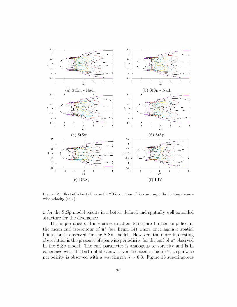
Figure 12 plots 2D isocontours for the streamwise fluctuating profiles forthe MULU. Once again an averaging is performed in time and along thespanwise direction. A clear distinction between the models with and withoutvelocity bias is again difficult to observe. However, on closer inspection,within the vortex bubbles, we can see that including velocity bias improvesthe agreement with the DNS by reducing the bubble size for the StSm modeland increasing it for the StSp model. The higher magnitude prediction alongthe centreline seen for the StSm - Nad model could be the result of an overallbias of the statistics and not due to an improvement in model performance -the presence of an inflection point in the profile further validates the modelinaccuracy. This error is corrected in the model with velocity bias. Thiscorrective nature of the bias is further analysed.

For the StSp model, the simulation without the bias has a larger recir-

26

culation zone or is ”over dissipative” and this is corrected by the bias. Thisresult supports the findings of (55) whose structure model, when employedin physical space, applies a similar statistical averaging procedure of square-velocity differences in a local neighbourhood. They found their model to alsobe over-dissipative in free-shear flows and did not work for wall flows as toomuch dissipation suppressed development of turbulence and had to be turnedoff in regions of low three-dimensionality. To achieve that (56) proposed thefiltered-structure-function model, which removes the large-scale fluctuationsbefore computing the statistical average. They applied this model with suc-cess to large-eddy simulation and analysis of transition to turbulence in aboundary layer. For the StSp model, which also displays this over dissipa-tion quality (without velocity bias), the correction appears to be implicitlydone by the velocity bias. Such a velocity correction is consistent with therecent findings of (19) who provided physical interpretations of the local cor-rective advection due to the turbulence inhomegeneity in the pivotal regionof the near wake shear layers where transition to turbulence takes place. Therecirculation length for all cases is tabulated in table 3. Data are obtainedfrom the centre-line velocity statistics shown in figure 11a. The tabulatedvalues further exemplify the corrective nature of the velocity bias where wesee an improved estimation of the recirculation length with the inclusion ofthe velocity bias. Also, a marginal improvement in statistical match similarto figure 11a is observed with the inclusion of the velocity bias for all lateralprofiles (not shown here). It can be concluded that the inclusion of velocitybias provides, in general, an improvement to the model.

The physical characteristics of the velocity bias (expressed henceforth asu∗ = 1

2∇ · a) are explored further. The bias u∗, having the same units as ve-

locity, can be seen as an extension or a correction to velocity. Extending thisanalogy, the divergence of u∗ is similar to “the divergence of a velocity field”.This is the case in the MULU where to ensure incompressibility, the diver-gence free constraints (eq. (5)) are necessary. The stability and statisticalaccuracy of simulations were improved with a pressure field calculated usingthe modified velocity u, i.e. when the weak incompressibility constraint wasenforced on the flow. This pressure field can be visualised as a true pressurefield unlike the Smagorinsky model where the gradients of the trace of thestress tensor are absorbed in an effective pressure field.

Stretching the u∗ and velocity analogy, we can also interpret the curl ofu∗ (∇× u∗) as vorticity or more specifically as a vorticity bias. The curl ofu∗ plays a role in the wake of the flow where it can be seen as a correction

27

−0.4

−0.2

0

0.2

0.4

0.6

0.8

1

0.5 1 1.5 2 2.5 3 3.5 4 4.5 5

<u>

Uc

x/D

PIV - ParnDNS

StSm - NadStSm

StSp - NadStSp

(a) < u >

0

0.02

0.04

0.06

0.08

0.1

0.12

0.14

0.5 1 1.5 2 2.5 3 3.5 4 4.5 5

<u′ u′ >

U2 c

x/D

PIV - ParnDNS

StSm - NadStSm

StSp - NadStSp

(b) < u′u′ >

Figure 11: Effect of velocity bias on centre-line mean (a) and fluctuating (b) streamwisevelocity behind the cylinder.

Table 3: Recirculation lengths with and without velocity bias.

Model PIV - Parn DNS StSm - Nad StSm StSp - Nad StSp

Lr/D 1.51 1.50 1.42 1.42 1.58 1.50

to the vorticity field. The divergence and curl of u∗ are features solely of theMULU and their characterisation defines the functioning of these models.

Figure 13 depicts the mean isocontour of ∇ · (u∗) = 0.02 for the twoMULU. This divergence function is included in the poisson equation for pres-sure calculation in order to enforce the weak incompressibility constraint. Inthe StSm model the contribution is strictly limited to within the shear layerwhile in the StSp model the spatial influence extends far into the downstreamwake. The stark difference in the spatial range could be due to the lack ofdirectional dissipation in the StSm model which is modelled on the classicSmagorinsky model. This modelling results in a constant diagonal auto cor-relation matrix, and the trace elements simplifying to a laplacian of a (∆a)for ∇ · (u∗). This formulation contains a no cross-correlation assumption(zero non-diagonal elements in the auto correlation matrix) as well as ignor-ing directional dissipation contribution (constant diagonal terms providesequal SGS dissipation in all three principle directions). These Smagorinskylike assumptions place a restriction on the form and magnitude of u∗ whichare absent in the StSp model. The existence of cross-correlation terms in

28

(a) StSm - Nad, (b) StSp - Nad,

(c) StSm. (d) StSp,

(e) DNS, (f) PIV,

Figure 12: Effect of velocity bias on the 2D isocontour of time averaged fluctuating stream-wise velocity (u′u′).

a for the StSp model results in a better defined and spatially well-extendedstructure for the divergence.

The importance of the cross-correlation terms are further amplified inthe mean curl isocontour of u∗ (see figure 14) where once again a spatiallimitation is observed for the StSm model. However, the more interestingobservation is the presence of spanwise periodicity for the curl of u∗ observedin the StSp model. The curl parameter is analogous to vorticity and is incoherence with the birth of streamwise vortices seen in figure 7, a spanwiseperiodicity is observed with a wavelength λ ∼ 0.8. Figure 15 superimposes

29

(a) StSm, (b) StSp.

Figure 13: 3D isocontour of the divergence of u∗ at ∇ · (u∗) = 0.02

(a) StSm, (b) StSp.

Figure 14: 3D isocontour of the curl of u∗ at ∇× (u∗) = 0.01 (for StSm), 0.05 (for StSp)

the isocontour of the curl of u∗ for the StSp model at ∇× (u∗) = 0.05 withthe mean DNS flow vorticity isocontour at Ω = 3. Figure 15a shows thesuperposition over a large spatial domain behind the cylinder. The outlinedbox within figure 15a indicates the area of zoom for figure 15b and figure15c. Figure 15b is the zoomed in view of the mean DNS vorticity isocontourat Ω = 3. The arrows in figure 15b indicate the points of match betweenthe mean vorticity peaks and the peaks in the mean curl isocontour of u∗ forthe StSp model. The superposed isocontours are shown in figure 15b. Thestructural match between the peaks of the two isocontours are satisfactorywith the periodic peaks in the curl of u∗ matching that of the noisier vorticity

30

isocontour. While clear periodicity is not observed for the mean vorticity,alternate peaks and troughs can be seen which match with the peaks inthe mean curl isocontour. The wavelength of this periodicity is comparablewith the spanwise wavelength of approximately 1D of mode B instabilitiesobserved by (53) for Re ∼ 270. The footprint of mode B instabilities islinked to secondary instabilities leading to streamwise vortices observed forRe ranging from 270 to ∼ 21000 (57). These results demonstrate the abilityof the spatial variance model to capture the essence of the auto-correlationtensor.

The regions of the flow affected by the auto-correlation term can be char-acterised by plotting the contours of SGS dissipation density ((∇u)a(∇u)T )of the MULU averaged in time and along the spanwise direction. Thesehave been compared with the dissipation densities for the Smag and DSmagmodels ((∇u)νt(∇u)T ) (see figure 17). A ‘reference’ dissipation density hasbeen obtained by filtering the DNS dissipation density at the cLES resolu-tion (see figure 16e) and by plotting the difference. The StSp model densitymatches best with the DNS compared with all other models - a larger spatialextent and a better magnitude match for the dissipation density is observed.The high dissipation density observed just behind the recirculation zone iscaptured only by the StSp model while all Smag models under-predict thedensity in this region. The longer recirculation zone for Smag model canbe observed in the density contours. A few important questions need to beaddressed here: firstly, the Smag model is known to be over-dissipative, how-ever, in the density contours, a lower magnitude is observed for this model.This is a case of cause and effect where the over-dissipative nature of theSmag model smooths the velocity field thus reducing the velocity gradientswhich inversely affects the value of the dissipation density. Secondly, in thestatistical comparison only a marginal difference is observed especially be-tween the DSmag and StSp models while in the dissipation density contourswe observe considerable difference. This is because the statistical profilesare a result of contributions from the resolved scales and the sub-grid scales.The dissipation density contours of figure 17 represent only a contribution ofthe sub-grid scales, i.e. the scales of turbulence characterised by the model.Thus, larger differences are observed in this case due to focus on the scalesof model activity. Finally, we observe in figure 9 that within the vortexbubbles behind the cylinder the MULU perform better than the Smag orDSmag models. For the StSp model, this improvement is associated withthe higher magnitude seen within this region in the SGS dissipation density.

31

(a) Full scale view of the isocontour superposition with the outlined zoom area

(b) Zoomed in view of the DNS meanvorticity isocontour

(c) Zoomed in view of the isocontour su-perposition

Figure 15: 3D isocontour superposition of the mean curl of u∗ (blue) for the StSp modelat ∇× (u∗) = 0.05 with the mean vorticity (yellow) for DNS at Ω = 3

For the StSm model, no such direct relation can be made with the SGS dis-sipation density. However, when we look at the resolved scale dissipation((∇u)ν(∇u)T ) for the models (see figure 16), a higher density is observed inthe vortex bubbles for this model. For the classical models high dissipationis observed mainly in the shear layers. As the kinematic viscosity (ν) for allmodels is the same, the density maps are indicative of the smoothness of thevelocity gradient. For the classical models, we see a highly smoothed field

32

while for the MULU, we see higher density in the wake. This difference couldinduce the isocontour mismatch seen in figure 9. These results are consistentwith the findings of (19), who applied the MULU in the context of reducedorder model and observed that MULU plays a significant role in the verynear wake where important physical mechanisms take place.

(a) Smag, (b) DSmag,

(c) StSm, (d) StSp,

(e) DNSo−f ,

Figure 16: Sub-grid scale dissipation density in the wake of the cylinder. o stands for theoriginal DNS dissipation and f stands for filtered (to cLES resolution) DNS dissipation.

For the MULU, the SGS contributions can be split into velocity bias(u∇T (−1

2∇ · a) and dissipation (1

2

∑ij ∂xi(aij∂xju)). Figure 18 shows the

contribution of the two via 3D isocontours (dissipation in yellow and velocitybias in red). The contribution of velocity bias is limited for the StSm modelas expected while in the StSp model it plays a larger role. Velocity biasin StSp model is dominant in the near wake of the flow especially in andaround the recirculation zone. It is important to outline that this is the

33

(a) Smag, (b) DSmag,

(c) StSm, (d) StSp,

Figure 17: Resolved scale dissipation density in the wake of the cylinder for each model.

region where a statistical mismatch is observed for Smag statistics which arepossibly corrected by the velocity bias in the StSp model.

Under the context of cLES, the statistical accuracy and stability of theMULU have been established with this study to be comparable, if not bet-ter, than the dynamic Smagorinsky model. The aim of performing cLES isto reduce the computational cost of simulations and hence opening neweravenues of research. This necessitates a study of the computational require-ment for each model (see table 4). All simulations were performed with thesame hardware and the simulation time, presented in table 4, is the time periteration for each model averaged over two simulations of 50 time-steps each.W/o model LES or under resolved DNS is the fastest as there is no extramodel calculations involved. For the cLES, MULU are computationally moreexpensive than classic Smagorinsky model as they involve calculation of bothSGS dissipation and the velocity bias terms - this leads to a marginally in-creased cost for the StSm model compared to the Smag model. The StSpmodel is roughly twice (∼ 1.98) as expensive as Smag models due to sta-tistical variance calculations for a performed over a local neighbourhood.However, the slight increase in computational cost is off-set by the statisticalimprovements of the StSp model over the Smag model. The cost of perform-ing the StSp model is 37% the cost of the DSmag model. This highlights

34

(a) StSm, (b) StSp,

Figure 18: 3d SGS contribution iso-surface along the primary flow direction (x) withdissipation iso-surface in yellow (at 0.002) and velocity bias in red (at 0.001)

Table 4: Computational cost [s] per iteration for each model.

Model w/o model Smag DSmag StSm StSp

Computational cost [s/iteration] 1.34 2.877 15.15 3.654 5.711

the most important feature of the StSp model - the model captures accu-rately the statistics at only 0.37 the cost of performing the DSmag model.However, it is important to note that while the computational cost for theSmagorinsky models stay fixed despite changes in model parameters, the costfor the StSp model strictly depends on the size of the local neighbourhoodused. A smaller neighbourhood reduces the simulation cost but could lead toloss of accuracy and vice versa for a larger neighbourhood. The definition ofan optimal local neighbourhood is one avenue of future research that couldbe promising. StSm model, which also provides comparable improvement onthe classic Smag model, can be performed at 24% the cost of the DSmagmodel. Thus, the MULU provide a low cost (2/3rd reduction) alternativeto the dynamic Smagorinsky model while improving the level of statisticalaccuracy.

35

5. Conclusion

In this study, cylinder wake flow in the transitional regime was simulatedin a coarse mesh construct using the formulation under location uncertainty.The simulations were performed on a mesh 54 times coarser than the DNSstudy. The simulation resolution is of comparable size with PIV resolution -this presents a useful tool for performing DA where in disparity between thetwo resolutions can lead to difficulties.

This study focused on the MULU whose formulation introduces a veloc-ity bias term in addition to the SGS dissipation term. These models werecompared with the classic and dynamic Smagorinsky model. The MULUwere shown to perform well with a coarsened mesh - the statistical accuracyof the spatial variance based model was, in general, better than the othercompared models. The spatial variance based model and DSmag model bothcaptured accurately the volatile recirculation length. The 2D streamwise ve-locity isocontours of the MULU matched better with the DNS reference thanthe Smagorinsky models. Additionally, the physical characterisation of theMULU showed that the velocity bias improved the statistics - considerablyin the case of the StSp model. The analogy of the velocity bias with velocitywas explored further through divergence and curl functions. The spanwiseperiodicity observed at low Re in literature was observed at this higher Rewith the StSp model through the curl of u∗ (analogous with vorticity) andthrough mean vorticity albeit noisily. The SGS contribution was comparedwith Smagorinsky models and the split of the velocity bias and dissipationwas also delineated through isocontours.

The authors show that the performance of the MULU under a coarsemesh construct could provide the necessary computational cost reductionneeded for performing LES of higher Re flows. The higher cost of the StSpmodel compared with Smagorinsky, is compensated by the improvement inaccuracy obtained at coarse resolution. In addition, the StSp model per-forms marginally better than the currently established DSmag model at just37% the cost of the DSmag model. This cost reduction could pave the wayfor different avenue of research such as sensitivity analyses, high Reynoldsnumber flows, etc. Of particular interest is the possible expansion of DataAssimilation studies from the currently existing 2D assimilations (14) or lowRe 3D assimilations (58) to a more informative 3D assimilation at realisticRe making use of advanced experimental techniques such as tomo-PIV. Alsoand more importantly, the simplistic definition of the MULU facilitate an

36

easy variational assimilation procedure.

6. Acknowledgements

The authors would like to thank EPSRC for the computational time madeavailable on the UK supercomputing facility ARCHER via the UK Turbu-lence Consortium (EP/L000261/1).

7. Bibliography

[1] A. A. Townsend, Momentum and Energy Diffusion in the TurbulentWake of a Cylinder, Proc. Math. Phys. Eng. Sci. 197 (1048) (1949)124–140. doi:10.1098/rspa.1949.0054.URL http://rspa.royalsocietypublishing.org/cgi/doi/10.

1098/rspa.1949.0054

[2] A. A. Townsend, The fully developed wake of a circular cylinder, Aust.J. Chem. 2 (4) (1949) 451–468.

[3] S. Singh, S. Mittal, Energy spectra of flow past a circular cylinder, Int.J. Comput. Fluid Dyn. 18 (8) (2004) 671–679.URL http://www.tandfonline.com/doi/abs/10.1080/

10618560410001730278

[4] A. Kravchenko, P. Moin, Numerical studies of flow over a circu-lar cylinder at Re[sub D]=3900, Phys. Fluids 12 (2) (2000) 403.doi:10.1063/1.870318.URL http://scitation.aip.org/content/aip/journal/pof2/12/

2/10.1063/1.870318

[5] S. Dong, G. Karniadakis, DNS of flow past a stationary andoscillating cylinder at, J. Fluids Struct. 20 (4) (2005) 519–531.doi:10.1016/j.jfluidstructs.2005.02.004.URL http://linkinghub.elsevier.com/retrieve/pii/

S0889974605000381

[6] X. Ma, G. Karamanos, G. Karniadakis, Dynamics and low-dimensionality of a turbulent near wake, J. Fluid Mech. 410 (2000)29–65.URL http://journals.cambridge.org/abstract_

S0022112099007934

37

[7] P. Parnaudeau, J. Carlier, D. Heitz, E. Lamballais, Experimental andnumerical studies of the flow over a circular cylinder at Reynolds num-ber 3900, Phys. Fluids 20 (8) (2008) 085101. doi:10.1063/1.2957018.URL http://scitation.aip.org/content/aip/journal/pof2/20/

8/10.1063/1.2957018

[8] P. Beaudan, P. Moin, Numerical experiments on the flow past a circularcylinder at sub-critical Reynolds number, Stanford Univ. Ca Thermo-sciences Div.

[9] L. M. Lourenco, C. Shih, Characteristics of the plane turbulent nearwake of a circular cylinder, A particle image velocimetry study.

[10] R. Mittal, P. Moin, Suitability of Upwind-Biased Finite DifferenceSchemes for Large-Eddy Simulation of Turbulent Flows, AIAA Jour-nal 35 (8) (1997) 1415–1417. doi:10.2514/2.253.URL http://arc.aiaa.org/doi/abs/10.2514/2.253

[11] J. Smagorinsky, General circulation experiments with the primitiveequations, Mon. Weather Rev. 91 (3) (1963) 99–164.URL http://www.ewp.rpi.edu/hartford/~ferraj7/ET/Other/

References/Gawronski/LES/Smagorinsky1963.pdf

[12] J. Meyers, P. Sagaut, On the model coefficients for the standard andthe variational multi-scale Smagorinsky model, J. Fluid Mech. 569(2006) 287. doi:10.1017/S0022112006002850.URL http://www.journals.cambridge.org/abstract_

S0022112006002850

[13] B. Combes, D. Heitz, A. Guibert, E. Memin, A particle filter toreconstruct a free-surface flow from a depth camera, Fluid Dyn. Res.47 (5) (2015) 051404.URL http://iopscience.iop.org/article/10.1088/0169-5983/

47/5/051404/meta

[14] A. Gronskis, D. Heitz, E. Memin, Inflow and initial conditions for directnumerical simulation based on adjoint data assimilation, J. Comput.Phys. 242 (2013) 480–497. doi:10.1016/j.jcp.2013.01.051.URL http://linkinghub.elsevier.com/retrieve/pii/

S0021999113001290

38

[15] Y. Yang, C. Robinson, D. Heitz, E. Memin, Enhanced ensemble-based4dvar scheme for data assimilation, Comput. Fluids 115 (2015) 201–210.doi:10.1016/j.compfluid.2015.03.025.URL http://linkinghub.elsevier.com/retrieve/pii/

S0045793015000985

[16] E. Memin, Fluid flow dynamics under location uncertainty,Geophys. Astrophys. Fluid Dynam. 108 (2) (2014) 119–146.doi:10.1080/03091929.2013.836190.URL http://www.tandfonline.com/doi/abs/10.1080/03091929.

2013.836190

[17] V. Resseguier, E. Memin, B. Chapron, Geophysical flows under locationuncertainty, part I: Random transport and general models, Geophys.Astrophys. Fluid Dynam. 11 (3) (2017) 149–176.

[18] S. K. Harouna, E. Memin, Stochastic representation of the Reynoldstransport theorem: revisiting large-scale modeling, Comput. Flu-idsdoi:10.1016/j.compfluid.2017.08.017.URL http://linkinghub.elsevier.com/retrieve/pii/

S0045793017302797

[19] V. Resseguier, E. Memin, D. Heitz, B. Chapron, Stochastic modellingand diffusion modes for proper orthogonal decomposition modelsand small-scale flow analysis, J. Fluid Mech. 826 (2017) 888–917.doi:10.1017/jfm.2017.467.URL https://www.cambridge.org/core/product/identifier/

S0022112017004670/type/journal_article

[20] A. Bensoussan, R. Temam, Equations stochastiques du type Navier-Stokes, J. Funct. Anal. 13 (2) (1973) 195–222.

[21] P. J. Mason, D. J. Thomson, Stochastic backscatter in large-eddy sim-ulations of boundary layers, J. Fluid Mech. 242 (1992) 51–78.

[22] U. Schumann, Stochastic backscatter of turbulence energy and scalarvariance by random subgrid-scale fluxes, Proc. R. Soc. A 451 (1995)293–318.

[23] R. H. Kraichnan, The structure of isotropic turbulence at very highReynolds numbers, J. Fluid Mech. 5 (04) (1959) 497–543.

39

URL http://journals.cambridge.org/abstract_

S0022112059000362

[24] C. Leith, Atmospheric predictability and two-dimensional turbulence, J.Atmos. Sci. 28 (2) (1971) 145–161.

[25] J. P. Laval, B. Dubrulle, J. C. McWilliams, Langevin models of turbu-lence: Renormalization group, distant interaction algorithms or rapiddistortion theory?, Phys. Fluids 15 (5) (2006) 1327–1339.

[26] R. Kraichnan, Convergents to turbulence functions, J. Fluid Mech. 41(1970) 189–217.

[27] B. Sawford, Generalized random forcing in random-walk models ofturbu-, Phys. Fluids 29 (1986) 3582–3585.

[28] D. Haworth, S. Pope, A generalized langevin model for turbulent flows.,Phys. Fluids 29 (1986) 387–405.

[29] S. Pope, Lagrangian pdf methods for turbulent flows, Annu. Rev. FluidMech 26 (1994) 23–63.

[30] S. Pope, Turbulent flows, Cambridge University Press, 2000.

[31] J. M. MacInnes, F. V. Bracco, Stochastic particle dispersion modelingand the tracer-particle limit, Phys. Fluids A: Fluid Dyn. 4 (12) (1992)2809. doi:10.1063/1.858337.URL http://scitation.aip.org/content/aip/journal/pofa/4/

12/10.1063/1.858337

[32] H. Kunita, Stochastic Flows and Stochastic Differential Equations, Cam-bridge University Press, 1990.

[33] V. Resseguier, E. Memin, B. Chapron, Geophysical flows under loca-tion uncertainty, Part II: Quasigeostrophic models and efficient ensemblespreading, Geophys. Astrophys. Fluid Dynam. 11 (3) (2017) 177–208.

[34] V. Resseguier, E. Memin, B. Chapron, Geophysical flows under locationuncertainty, Part III: SQG and frontal dynamics under strong turbu-lence, Geophys. Astrophys. Fluid Dynam. 11 (3) (2017) 209–227.

40

[35] D. D. Holm, Variational principles for stochastic fluid dynamics,Proc. Math. Phys. Eng. Sci. 471 (2176) (2015) 20140963–20140963.doi:10.1098/rspa.2014.0963.URL http://rspa.royalsocietypublishing.org/cgi/doi/10.

1098/rspa.2014.0963

[36] D. Crisan, F. Flandoli, D. D. Holm, Solution properties of a 3d stochasticEuler fluid equation, arXiv preprint arXiv:1704.06989.URL https://arxiv.org/abs/1704.06989

[37] C. J. Cotter, G. A. Gottwald, D. D. Holm, Stochastic partial differentialfluid equations as a diffusive limit of deterministic Lagrangian multi-timedynamics, arXiv preprint arXiv:1706.00287.URL https://arxiv.org/abs/1706.00287

[38] D. K. Lilly, The representation of small scale turbulence in numericalsimulation experiments, Proc. IBM Sci. Compt. Symp. Environ. Sci.(1967) 195–210.

[39] M. Germano, U. Piomelli, P. Moin, W. Cabot, A dynamic subgrid-scaleeddy viscosity model, Phys. Fluids A: Fluid Dyn. 3 (7) (1991) 1760.doi:10.1063/1.857955.URL http://scitation.aip.org/content/aip/journal/pofa/3/7/

10.1063/1.857955

[40] E. R. Van Driest, The problem of aerodynamic heating, Aero. Engg.Rev. 15 (10) (1956) 26–41.

[41] V. Yakhot, S. A. Orszag, Renormalization group analysis of turbulence.I. Basic theory, J. Sci. Comput. 1 (1) (1986) 3–51.URL http://link.springer.com/article/10.1007/BF01061452

[42] M. Breuer, N. Jovicic, K. Mazaev, Comparison of DES, RANS andLES for the separated flow around a flat plate at high incidence, Int. J.Numer. Meth. Fluids 41 (4) (2003) 357–388.URL http://onlinelibrary.wiley.com/doi/10.1002/fld.445/

full

[43] H. Ouvrard, B. Koobus, A. Dervieux, M. V. Salvetti, Classical andvariational multiscale LES of the flow around a circular cylinder

41

on unstructured grids, Comput. Fluids 39 (7) (2010) 1083–1094.doi:10.1016/j.compfluid.2010.01.017.URL http://linkinghub.elsevier.com/retrieve/pii/

S0045793010000319

[44] S. Laizet, E. Lamballais, High-order compact schemes for in-compressible flows: A simple and efficient method with quasi-spectral accuracy, J. Comput. Phys. 228 (16) (2009) 5989–6015.doi:10.1016/j.jcp.2009.05.010.URL http://linkinghub.elsevier.com/retrieve/pii/

S0021999109002587

[45] S. Lele, Compact finite difference schemes with spectral-like resolution,J. Comput. Phys. 103 (1) (1992) 16–42.

[46] R. Gautier, S. Laizet, E. Lamballais, A DNS study of jet control withmicrojets using an immersed boundary method, Int. J. Comput. FluidDyn. 28 (6-10) (2014) 393–410. doi:10.1080/10618562.2014.950046.URL http://www.tandfonline.com/doi/abs/10.1080/10618562.

2014.950046

[47] L. C. Pinto, E. B. C. Schettini, J. H. Silvestrini, Numerical analysisof the immersed boundary method applied to the flow around aforced oscillating cylinder, J. Phys. Conf. Ser. 296 (2011) 012011.doi:10.1088/1742-6596/296/1/012011.URL http://stacks.iop.org/1742-6596/296/i=1/a=012011?key=

crossref.596e99f672722522c1ffb573038e4aff

[48] S. Laizet, N. Li, Incompact3d: A powerful tool to tackle turbulenceproblems with up to O(105) computational cores, Int. J. Numer. Meth.Fluids 67 (11) (2011) 1735–1757. doi:10.1002/fld.2480.URL http://doi.wiley.com/10.1002/fld.2480

[49] O. Metais, M. Lesieur, Spectral large-eddy simulation of isotropicand stably stratified turbulence, J. Fluid Mech. 239 (1992) 157.doi:10.1017/S0022112092004361.URL http://www.journals.cambridge.org/abstract_

S0022112092004361

42

[50] C. Norberg, LDV measurements in the near wake of a circular cylinder,in: Proceedings of the Conference on Bluff Body Wakes and Vortex-Induced Vibration, Cornell Univesity, Ithaca, NY, 1998, Washington,D.C., 1998, pp. 1–12.

[51] T. Corpetti, D. Heitz, G. Arroyo, E. Mmin, A. Santa-Cruz, Fluid exper-imental flow estimation based on an optical-flow scheme, Experimentsin Fluids 40 (1) (2006) 80–97. doi:10.1007/s00348-005-0048-y.URL http://link.springer.com/10.1007/s00348-005-0048-y

[52] L. Ong, J. Wallace, The velocity field of the turbulent very near wakeof a circular cylinder, Exp. Fluids 20 (6) (1996) 441–453.URL http://link.springer.com/article/10.1007/BF00189383

[53] C. H. K. Williamson, Vortex dynamics in the cylinder wake, Annu. Rev.Fluid Mech. 28 (1996) 477–539.

[54] C. Chyu, D. Rockwell, Near-wake structure of an oscillating cylinder:effect of controlled shear-layer vortices, J. Fluid Mech. 322 (1996)21–49.URL http://journals.cambridge.org/abstract_

S0022112096002698

[55] M. Lesieur, P. Comte, Y. Dubief, E. Lamballais, O. Metais, S. Ossia,From two-point closures of isotropic turbulence to LES of shear flows,Flow Turbul. Combust. 63 (1-4) (2000) 247–267.URL http://link.springer.com/article/10.1023/A:

1009900723783

[56] F. Ducros, P. Comte, M. Lesieur, Large-eddy simulation of transition toturbulence in a boundary layer developing spatially over a flat plate, J.Fluid Mech. 326 (1996) 1–36.

[57] B. Bays-Muchmore, A. Ahmed, On streamwise vortices in turbulentwakes of cylinders, Phys. Fluids A: Fluid Dyn. 5 (2) (1993) 387–392.doi:10.1063/1.858862.URL http://aip.scitation.org/doi/10.1063/1.858862

[58] C. Robinson, Image assimilation techniques for Large Eddy Scale mod-els : Application to 3d reconstruction, (doctoral thesis, Universite deRennes 1, Rennes (2015).

43