Received: 2 October 2017

IOTC–2017–WPTT19–37

1

CPUE STANDARDISATIONS OF THE SEYCHELLES INDIAN OCEAN

LONGLINE FLEET 2004–2015

PREPARED BY: IOTC SECRETARIAT1. 28 SEPTEMBER 2017

1 Dan.fu@fao.org, Lucas, J., Assan, C., Govinden, R., Chassot, E.

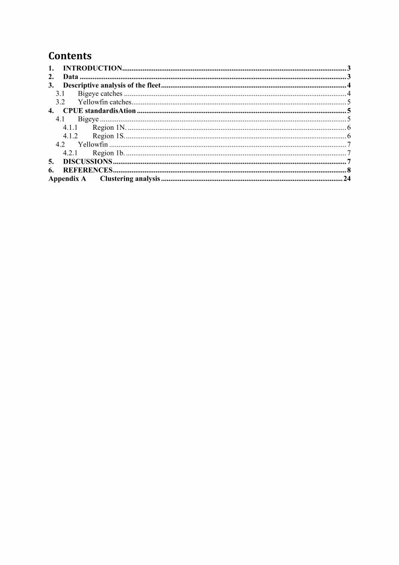
Contents 1. INTRODUCTION ......................................................................................................................... 3 2. Data ................................................................................................................................................ 3 3. Descriptive analysis of the fleet .................................................................................................... 4

3.1 Bigeye catches ........................................................................................................................ 4 3.2 Yellowfin catches .................................................................................................................... 5

4. CPUE standardisAtion ................................................................................................................. 5 4.1 Bigeye ..................................................................................................................................... 5

4.1.1 Region 1N. ...................................................................................................................... 6 4.1.2 Region 1S. ....................................................................................................................... 6

4.2 Yellowfin ................................................................................................................................ 7 4.2.1 Region 1b. ....................................................................................................................... 7

5. DISCUSSIONS .............................................................................................................................. 7 6. REFERENCES .............................................................................................................................. 8 Appendix A Clustering analysis .................................................................................................. 24

2

SUMMARY

We analysed Seychelles’ industrial longline operational catch and effort data to describe and

characterize the temporal and spatial patterns of the fishery. The focus is on the tropical tuna species

bigeye and yellowfin tuna, but information on other species is included.. We conducted standardised

CPUE analysis for Seychelles industry longline fishery data from 2001 to 2015. Cluster analysis was

used to classify longline sets in relation to species composition of the catches to understand whether

cluster analysis could identify distinct fishing strategies. Bigeye and Yellowfin tuna CPUE

standardization for core regions were presented. All analyses were based on the approaches used by the

collaborative workshop of longline data and CPUE standardization for bigeye and yellowfin tuna held

in July 2016 in Busan.

For bigeye tuna, CPUE Standardisations were conducted to the western tropical regions 1N and 1S

separately. The lognormal models fitted to the non-zeros sets resulted in very similar trends in both

regions, and the standardised CPUE index has declined between 2004 and 2010 with strong inter-annual

fluctuations. The standardised catch rates peaked around 2012 when the fleet returned to the fishing

ground in the western Indian Ocean, and the catch rates between 2013 and 2015 were on average lower

than those in the mid-2000s (before the piracy threat period (2008 -2011).

For yellowfin tuna, CPUE standardisations were conducted in region 1b. The delta-lognormal model

was applied and the YFT region 1S appears adequate and consistent trends were estimated from both

the binomial and lognormal part of the model, suggesting that the population in the region may have

declined between 2004 and 2010.

3

1. INTRODUCTION

A number ccollaborative studies were carried out in 2015 and 2016 to explore factors affecting the

catch rates of Japanese, Taiwanese, and Korean longline fleets fishing for bigeye, yellowfin, and

albacore tunas in the Indian Ocean (Hoyle et al. 2015a, b, 2016a,b). Methods for the standardisation of

joint longline catch and effort datasets from distant water fishing nations (DWFNs) were developed that

incorporate an innovative approach in identifying target changes. The standardised CPUE indices have

been used as the index of abundance in the most recent IOTC stock assessments for albacore (Langley

& Hoyle, 2016), bigeye (Langley 2016a), and yellowfin tuna (Langley 2016b). The Working Party on

Tropical Tunas (WPTT) has recommended the method to be further developed to improve estimates of

abundance, to investigate the feasibility of extending the methodology to include Seychelles data.

In July 2017, a workshop was held between national scientists and an independent scientist, Dr. Simon

Hoyle with expertise in Japanese, Taiwanese, Korean and Seychelles longline fleets to develop joint

CPUE indices for bigeye and YFT, as well as indices for individual fleet, based on data from the

Japanese Taiwanese, Korean, and Seychelles fleets (IOTC 2017). This report provides information and

analysis of the Seychelles longline fleet. Complementary reports address the Taiwanese (Yeh et al.

2017), Korean (Lee et.al. 2017) fleets, Japanese (Matsumoto 2017) fleet. A further report (Hoyle et al.

2017b) addresses the main objectives of the study.

2. DATA

The Seychelles industrial longline fleet consists of large, long distance vessels, of Taiwanese origin,

licensed to operate inside the Seychelles EEZ and target various tuna species. Compared to the main

DWLN fleets, the Seychelles industrial longline fleet has a shorter history and a smaller geographic

coverage, but has a reasonably consistent fishing pattern and targeting strategies, which may therefore

provide an important independent source of information.

Seychelles registered vessels are under obligation to submit a logbook wherever they operate for the

whole validity of registration period. The logbook provides all fishing trip information including daily

activities, catches, and effort information. The data used in the report are maintained by Seychelles

Fishing Authority (SFA), and include 78894 sets from 664 trips covering 2001–2015. The data before

2004 are not complete – over 50% of logbooks are missing; the number of logbook return has increased

remarkably since 2004, with an average of over 90% logbook coverage.

Each record corresponds to an individual set; key variables include trip/set code, vessel ID, location,

set-time, number of hooks, catch in both numbers and weight by species. Location by latitude and

longitude are usually recorded to high precision, but latitude and longitude were reported at 1 degree

resolution for about 10% of total records. The data is thoroughly verified and validated following which

missing hooks and catches in number are estimated. No further grooming is performed in this analysis.

Numbers of hooks between float (HBF) are not available in the dataset: vessels started to record HBF

as from 2015.

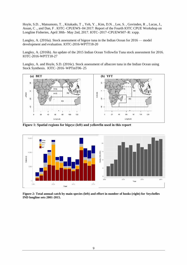
Each set was allocated to a yellowfin region (consistent with the definitions in the yellowfin stock

assessment, Langley 2016a) and a bigeye region (consistent with the bigeye assessment, Langley

2016b). The bigeye region includes a western equatorial region, which is further divided into the north

(R1N) and south regions (R1S) at the equator, eastern equatorial region (R2) and southern region (R3)

(Figure 1–left). The yellowfin region consists of five regions (Figure 1–right). Langley (2016b) adopted

a four region model structure for the yellow assessment, combining the Arabian Sea (region 1a) and

western equatorial region (region 1b), but the two sub-regions were retained for the definition of

spatially distinct fisheries that operate in each area. In analysing Seychelles data, we retained the two

sub regions, as the Arabian Sea fishery operated differently (it has a much shorter duration and a much

4

higher catch rates than the western equatorial region). Data outside these locations were not considered

in the analysis (about 3% of sets).

Taiwanese longline fleet developed the oil fish fishery in the south-west Indian Ocean since 2006. This

is a new fishery with significantly lower catchability for tunas and the Taiwanese CPUE in southern

regions is affected by the rapid growth of this fishery (Hoyle et al. 2015b). In the Seychelles logbook

the species was recorded under code ‘MZZ’ which also included other unidentified species. From 2015,

Oil fish is recorded under a separate code ‘OIL’. In the analysis, OIL in 2015 was combined with MZZ.

Seychelles longline vessels are known to have been mostly targeting bigeye and yellowfin in the tropical

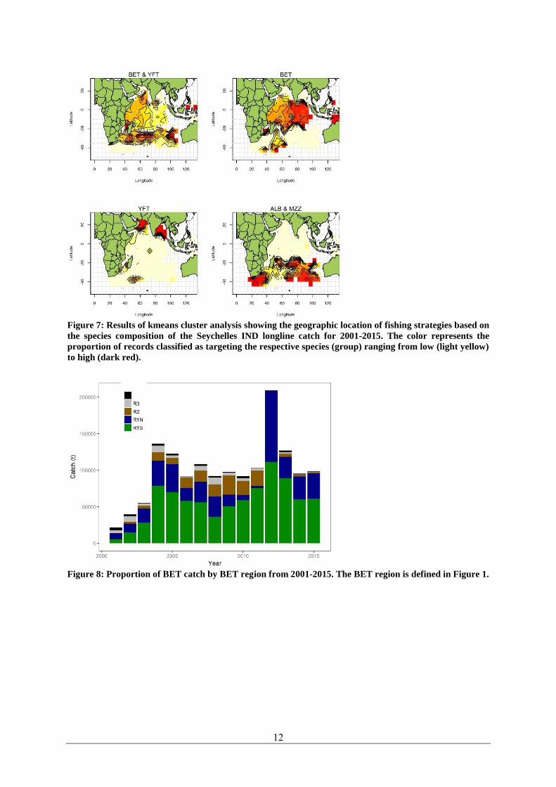
regions. As part of the joint analysis, we used the hierarchical clustering method to identify effort

associated with potentially different fishing strategies. The clustering was based on the Ward hclust

method and was performed separately by regions for both bigeye and yellowfin, to derive variable

representing targeting strategies to be included in the standardisation. Analyses used species

composition to group the data, and were performed on data aggregated by vessel-month to reduce the

variability, and therefore reduce misallocation of sets (IOTC 2015). The clustering applied to the whole

dataset indicates high YFT in the catch composition in the Arabian Sea, and high MZZ catch proportions

in the south-west of the Indian Ocean (Figure 7).

3. DESCRIPTIVE ANALYSIS OF THE FLEET

Information on annual total catch and effort are summarised in Table 1. With some fluctuations, the

bigeye tuna remained the dominant species caught by the Seychelles longline fleet, accounting for 49%

of the total catch between 2001 and 2015. Yellowfin and swordfish are the second and third most

dominant species, comprising 17% and 9% of the total catch, followed by MZZ (including OIL fish and

other unidentified species) 9%, ALB (4%), MAR (2%), and SHK (1%) (Figure 2–left). There has been

an apparent reduction in both effort and catch between 2008 and 2011 (Error! Reference source not

found.–right), due to the piracy in the West Indian Ocean. Over 20 million hooks per year were

deployed for the last three years (Table 1).

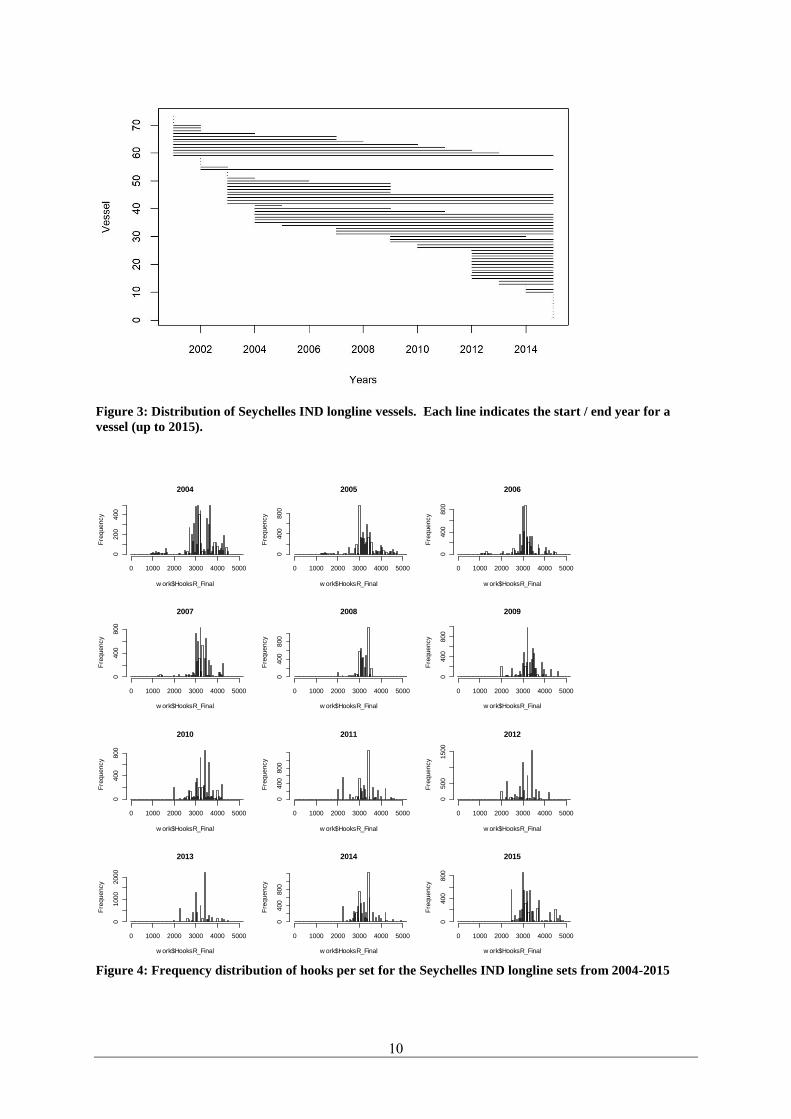
In total about 70 industrial longliners operated under Seychelles flag since 2001 (Figure 3), and there

are on average about 40 active vessels per year over the last 5 years. The number of hooks per set

typically ranged between 2000 and 4000, with very few sets outside this range (Figure 4). There has

been no apparent trend in the number of hooks per set overtime.

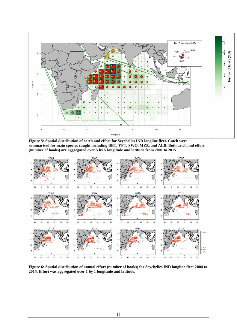
The fleet has been fishing mostly in the western equatorial region, with majority of the effort

concentrating between 10° north and 15° south latitude, and between 40° north and 70° longitude, where

the catches have been dominated by BET and YFT (Figure 5). The spatial distribution of fishing effort

was stable, except for a few changes: the fishing in the norther part of Indian Ocean appeared to have

stopped after 2007 and the vessel has not returned to the Arabian Sea; there has been little fishing effort

in the eastern Indian Ocean after 2010 (Figure 6). With the onset of the piracy threat in the late-2000s,

the activities of the fleet operating in the north-west Indian Ocean have been displaced or reduced. Since

2012 catches of tropical tunas appear to show signs of recovery – as a result of the reduction of the

threat of piracy and return of fleets and to the north-west Indian Ocean (Geehan et.al. 2015).

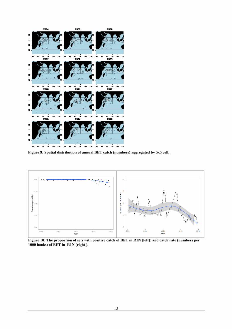
3.1 Bigeye catches

The annual bigeye catches were stable but the catch was almost doubled in 2012 when the fleets returned

to the north-west Indian Ocean, followed by a drop in catches to pre-2012 level in the recent years

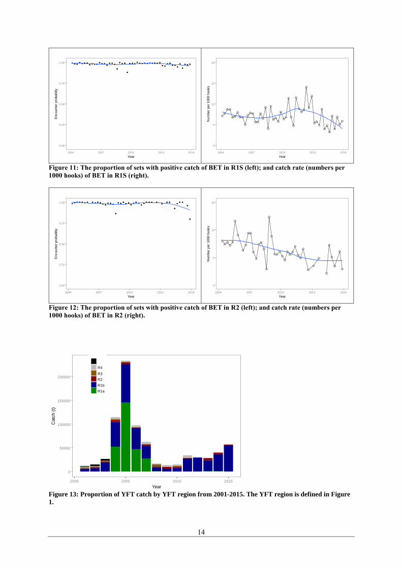
(Figure 8). Region 1S is the most important region in terms of BET catches for the Seychelles longline

fleet. The recent trend in annual catches in the region was influenced by piracy. The catch from region

1N was small but was reasonably stable except for the decrease before 2012. A significant proportion

of catches between 2004 and 2010 were taken from region 2, but the fishing in the eastern Indian Ocean

5

has been greatly reduced since 2010 (Figure 9). In tropical areas (1N, 1S, and 2) there were very few

sets that did not record any bigeye tuna in their reported catches, and the proportion of non-zero sets

per annum was close to 100%, except for a slight drop in the last few years (Figure 10Figure 11Figure 12

– left). In the western Indian Ocean (region 1N and 1S), the nominal catch rates had large seasonal

fluctuations with a peak in 2012, and declined in the last few years (Figure 10Figure 11–left). In the

eastern Indian Ocean, the nominal catch rates declined between 2004 and 2010 (Figure 10Figure 12–left).

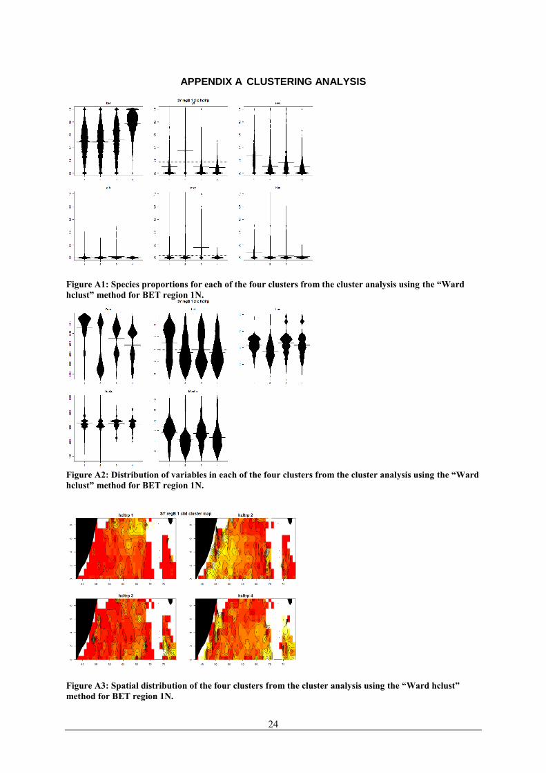
Clustering analysis showed that in both region 1N and 1S, all clusters are dominated by BET catches

(Appendix Figure A1–A4). In region 1N, cluster 4 has even higher BET proportions, and this cluster

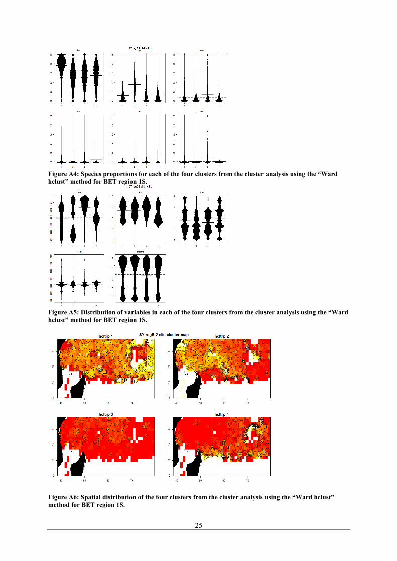
appears to be distributed on both the most eastern and western part of region 1N. In region 1S, cluster

1 has the highest BET proportions, and is distributed throughout region 1S.

3.2 Yellowfin catches

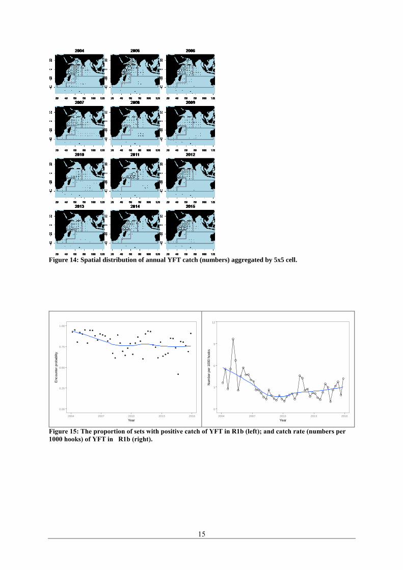
Large catches of YFT were recorded between 2004 and 2007 mostly contributed by the fishing in the

Arabian Sea (Figure 13) but the fleet has not fish in that region since 2007 (Figure 14). Lan et al. (2012)

showed the nominal CPUE of yellowfin in the Arabian Sea by the Taiwanese longline fishery was

usually 2–3 times higher than the average nominal CPUE in the Indian Ocean, especially after 1986,

when the Taiwanese adopted super-cold storage and operated more often with deep longlines, and

suggested that the may have been due to the distribution of and depth of yellowfin tuna as a result of

large-scale climatic oscillations patterns.

In region 1b, the annual proportion of non-zero yellowfin sets fluctuated around 70% to 90%, and has

declined between 2004 and 2010 (Figure 15–left). The nominal catch rates also followed a declining

trend during the same period (Figure 15–right).

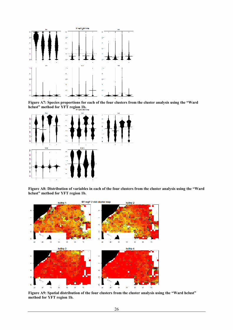
Clustering analysis showed that in region 1b all clusters are dominated by BET catches (Appendix

Figure A5–A6). Cluster 2 has relative high YFT catches and is distributed towards the western part of

region 1b; Cluster 3 has higher SWO catches and is mostly on the eastern-northern part of the region.

4. CPUE STANDARDISATION

The primary goal of CPUE standardization is to estimate a time series of relative abundance, and this

is accomplished by identifying and removing the effects of various sources of CPUE variation that are

attributable to causes other than changing abundance (e.g. changes in efficiency of the fleet due to

improvements in technology or changes in targeting practices). The analysis involves estimation and

presentation of annual time series of relative abundance using Generalized Linear Models (GLMs). The

GLMs estimate the effects of independent variables which are expected to influence catchability, such

that the effect of these variables can be removed to estimate a time series in which (ideally) the main

source of variability is changing abundance.

The analyses were based on the approaches used by the collaborative workshop of longline data and

CPUE standardization for bigeye and yellowfin tuna held in July 2017 in Busan. Analyses were

conducted separately for each region, and for bigeye and yellowfin. For the CPUE standardization, the

response variable considered for this study was catch per unit of effort (CPUE), measured as number of

fish per 1000 hooks deployed, the main factor explanatory variables considered include year-quarter,

vessel id, five by five latitude and longitude grid, and cluster.

4.1 Bigeye

CPUE Standardisations were conducted to bigeye region 1N and 1S separately. Region 2 was not

considered for this analysis because there was little fishing effort after 2010. For each region, a subset

6

of data was derived for the standardisation based on the following criteria:

Selecting vessels that fished at least two quarters, with a minimum of 10 sets

Selecting quarters that had a minimum 10 sets.

Selecting 5x5 grids that had a minimum of 10 sets

Relatively small values (compared to those adopted for the analysis of the main DWFN fleets which

has a much larger dataset) were chosen to define these thresholds to allow for more data to be included

in the standardisations.

As there were only a negligible amount of sets that did not catch any bigeye tuna in both regions, a

lognormal model was used and was fitted to the positive sets as follows:

ln(𝐶𝑃𝑈𝐸) ~ 𝑦𝑟𝑞𝑡𝑟 + 𝑣𝑒𝑠𝑠𝑖𝑑 + 𝑙𝑎𝑡𝑙𝑜𝑛𝑔5 + 𝑛𝑠(ℎ𝑜𝑜𝑘𝑠) + 𝑐𝑙 + 𝜖

The response variable, the log-transformed CPUE is defined to be the number of fish caught per 1000

hooks. The explanatory variables include year-quarter, vessel id, 5x5 grid cell, and cluster as categorical

variables. Number of hooks were included as a continuous variable with a natural spline with a knot 3.

In each region, two models were fitted, one with the cluster variable, and the other without the cluster

variable.

4.1.1 Region 1N.

Results from the standardisation models are shown in Figures 16–19. There is a modest declining trend

in the standardised indices (year effects) between 2004 and 2010 with very large seasonal fluctuations

(Figure 16). The large spike in 2011 is mostly because there is only a small amount of sets during the

piracy period. The index is also very high in 2012 when the fleet returned to the fishing ground. The

indices dropped after 2012 and declined to 2015 with large variations. Spatial variations in catch rates

appear to be small except for a few areas in the east of the region (>70 E) where high catch rates were

observed. The fishing efficiency appears to be similar among vessels with no obvious trend over time.

Cluster 4 (mostly dominated by bigeye catches, see Figure A1, Appendix A) has higher catch rates of

bigeye tuna than other clusters.

The residuals from the standardisation model appear to be negatively skewed, indicating some departure

from the assumption that the (log) catch rates are normally distributed. (Figure 17–left). An examination

of the residuals by covariates suggested that the residuals usually have heavy tails across most levels of

each variable (Figure 17–right). These patterns suggest there is probably a lack of fit to the data in the

standardisations and some further investigation is needed to improve the fits (such as the use of an

alternative transformation).

The influence plots (figure 18) show that the number of sets in cluster 4 (the cluster dominated bigeye

catches) has declined significantly in recent years, therefore including the cluster variable in the

standardisation will increase the recent indices, resulting a time series of abundance with less overall

decline. However, in the tropical area, the species composition is probably more likely to have reflected

the species abundance and availability rather than targeting strategy, therefore including the cluster

variable may have ‘washed up’ the biomass signal. An alternative model excluding the cluster variable

produced a slightly steeper decline in the overall abundance series. In the case, we consider that it is

probably more appropriate not to include the cluster variable in the standardisation of bigeye catch rates

for region 1N.

4.1.2 Region 1S.

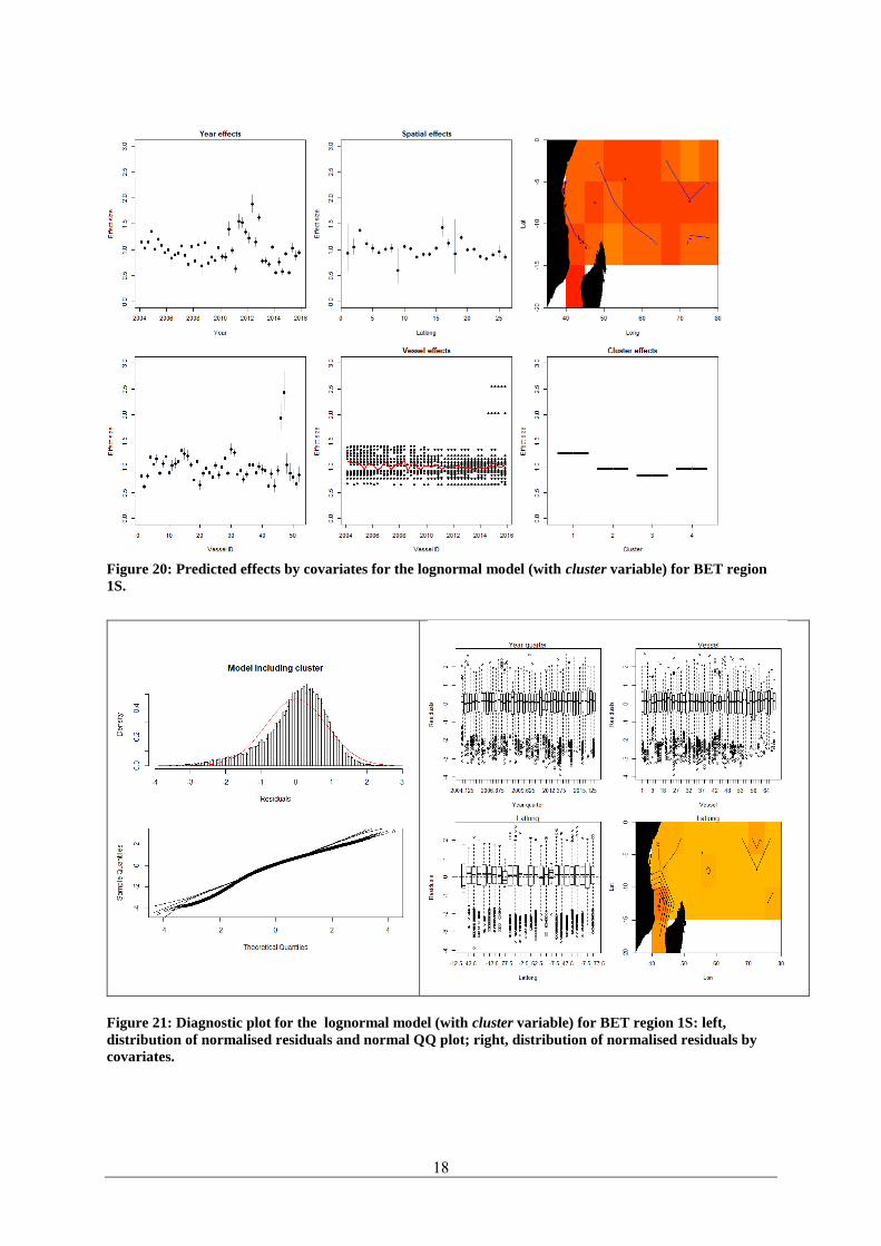
Results from the standardisation models are shown in Figures 20–23. Similar to region 1N, the

standardised CPUE in region 1S declined from 2004 to 2010, increased significantly in 2012, and

fluctuated to 2015 (Figure 20). There was little spatial variation in catch rates. The catch rates of most

7

vessels were similar except for a few vessels whose catch rates appear to be above the average. Cluster

1 has the highest proportions of bigeye catches (Figure A4, Appendix A), as shown in the estimated

cluster effects.

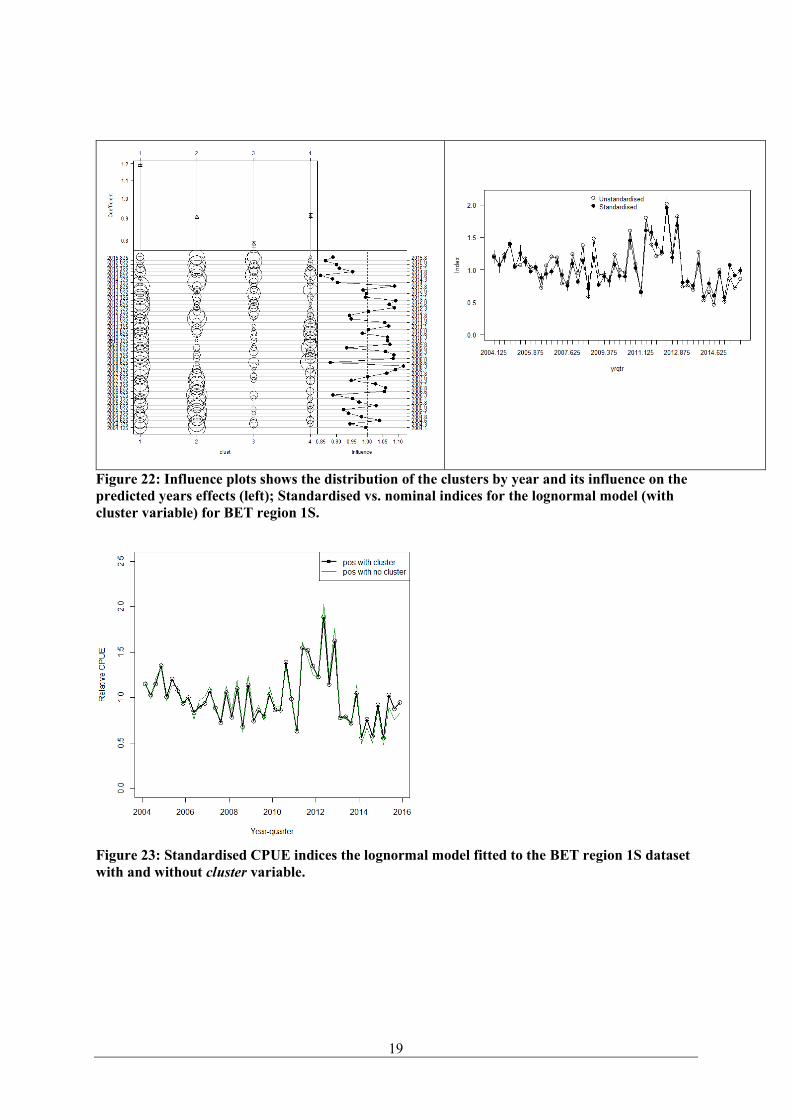
Similar to region 1N, there are some negative skewness in the distributions of residuals (Figure 21),

suggesting that the lognormal model is probably not adequate. The influence plots (Figure 22) led to a

similar conclusion as for the case of region 1N. As the number of sets in cluster 1 (the dominant bigeye

cluster) has reduced in recently years, including the cluster variable will produce higher CPUE indices

in recent years. The alternative model excluding the cluster variable produced a slightly steeper decline

in the overall abundance series. Therefore we consider that it is probably more appropriate not to include

the cluster variable in the standardisation of bigeye catch rates for region 1S.

4.2 Yellowfin

Because up to 30% of sets in region 1b caught zero yellowfin tuna, we applied the delta-lognormal

model for the standardisation (Lo et al. 1992; Maunder & Punt 2004), which used a binomial

distribution for the probability w of catch rate being zero and a probability distribution f(y), where y

was log(catch per 1000 hooks set) for non-zero (positive) catch rates.

• Binomial (𝐶𝑃𝑈𝐸 = 0)~ 𝑦𝑟𝑞𝑡𝑟 + 𝑣𝑒𝑠𝑠𝑖𝑑 + 𝑙𝑎𝑡𝑙𝑜𝑛𝑔5 + 𝑐𝑙 + 𝜖

• Lognormal log(𝐶𝑃𝑈𝐸)~ 𝑦𝑟𝑞𝑡𝑟 + 𝑣𝑒𝑠𝑠𝑖𝑑 + 𝑙𝑎𝑡𝑙𝑜𝑛𝑔5 + +𝑐𝑙 + 𝜖, for nonzero sets

The two models are integrated together to estimate an annual standardized time series. We also applied

a lognormal constant model:

• ln(𝐶𝑃𝑈𝐸𝑠 + 𝑘) ~ 𝑦𝑟𝑞𝑡𝑟 + 𝑣𝑒𝑠𝑠𝑖𝑑 + 𝑙𝑎𝑡𝑙𝑜𝑛𝑔5 + 𝑓(ℎ𝑜𝑜𝑘𝑠) + 𝑐𝑙 + 𝜖

where the constant k is equal to the lower 10th percentile of all non-zero CPUE observations

For the Delta-lognormal analyses, two models were fitted: one estimated the vessel effects, the other

excluded the vessel effects.

4.2.1 Region 1b.

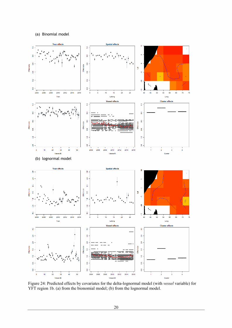
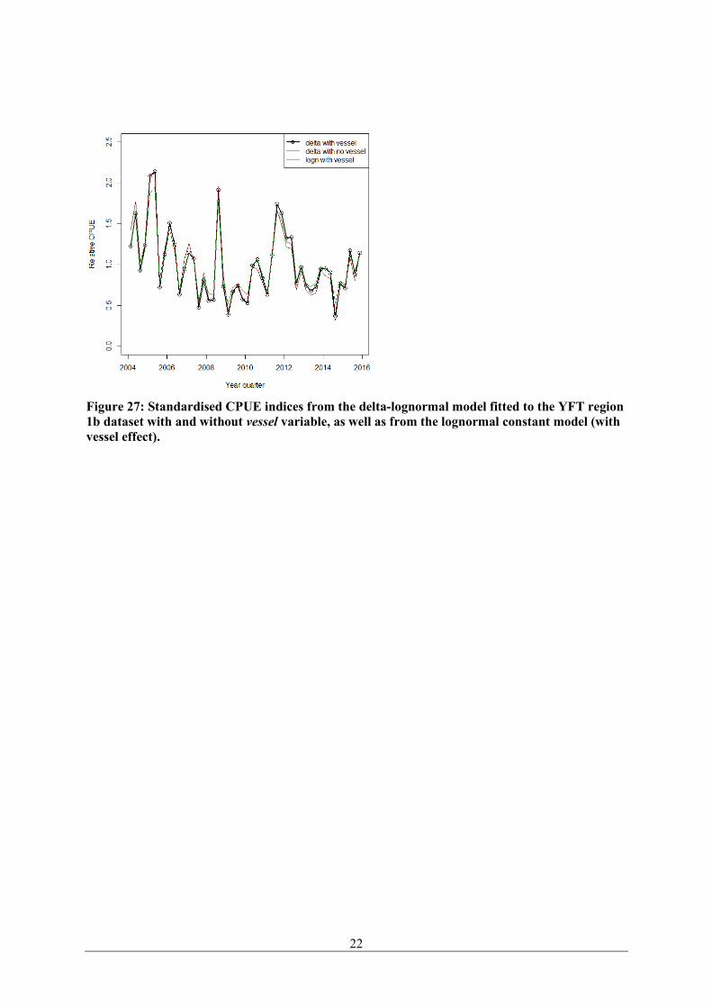
Results are shown in Figures 24–27. Both the binomial and lognormal models show a similar trend in

the year effects: the CPUE declined from 2004 to 2010, increased in 2011 and 2012, and remained flat

after 2012 (Figure 24). Estimated years effects in both models exhibited very large inter-annual

variations. Estimated effects of other covariates are also consistent between the binomial and lognormal

models. There appears to be some spatial variations in the probabilities of obtaining positive catches of

YFT. The overall efficiency of the fleet with respect to YFT catches have decreased overtime, therefore

including vessel effects in the standardisations process is important to separate the change of fishing

efficiency from abundance signals.

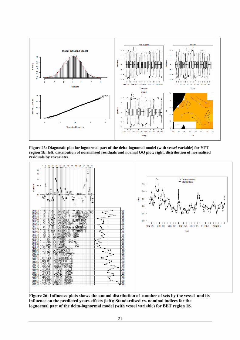
The residuals indicate that the model fitted the data very well and there is no obvious departure from

the normal assumption of the (log) catch rates (Figure 21). The influence plots suggested that overtime,

the vessel efficiency in catching YFT has been declining, which serves to increase the standardised

indices, suggesting that the abundance may not have declined as much as what was observed from the

unstandardized catch rates. Because there are generally good overlaps in fleet coverage overtime, the

vessels effects are likely to have been well estimated.

5. DISCUSSIONS

8

This is the first time Seychelles industrial longline data are used in the collaborative analysis to derive

the joint CPUE indices for BET and YFT. Compared to other DWFN, The Seychelles industrial

longline fleet has a much shorter catch history, and smaller spatial coverage. However, the fleet appears

to have a consistent fishing strategy, and therefore should be able to provide valuable and independent

information to the joint analysis.

The lognormal models fitted to the non-zeros sets for BET region 1N and 1S resulted in very similar

trends in both regions. There is a gently declining trend between 2004 and 2010 with strong inter-annual

fluctuations. The standardised catch rates peaked around 2012 when the fleet returned to the fishing

ground in the western Indian Ocean. The standardised catch rates between 2013 and 2015 were lower

than in the mid-2000s (before the piracy period). Langley (2016a) suggested that the differential in

CPUE in the region is correlated with the IODI: the strong positive IODI during 2006–2012 is correlated

with the higher CPUE, while the sharp decline in CPUE during 2013–2014 corresponded to generally

negative IODI (See Langley 2016a Figure 11).

The standardisation models for BET showed some lack of fit to the data, requiring further investigations

such as alternative transformation of the observations, or alternative error structures. For the Seychelles

industrial longline fleet operating in the tropical regions, the target strategies defined via the clustering

analysis based on species proportions may have only indexed species availability, therefore it may be

appropriate not to include the cluster variable for the standardisation in this region.

The delta-lognormal model applied to the YFT region 1S appears to be adequate. Consistent trends

were estimated from both the binomial and lognormal part of the model, suggesting that the population

in the region may have declined between 2004 and 2010.

6. REFERENCES

Seychelles fishing authority 2017. Annual report 2014, Victoria Mahe, Seychelles. 108 p.

Lan, K.W., Lee, M.A., Nishida, T., Lu, H.J., Weng, J.S., and Chang, Y. (2012). Environmental effects

on yellowfin tuna catch by the Taiwan longline fishery in the Arabian Sea, International Journal of

Remote Sensing, 33:23, 7491-7506, DOI: 10.1080/01431161.2012.685971

Geehan, J., Fiorellato, F., Pierre, L. 2015. REVIEW OF THE STATISTICAL DATA AND FISHERY

TRENDS FOR TROPICAL TUNAS. IOTC–2016–WPTT18–07: 47pp.

Hoyle, S. D., Chang, Y., Yeh, Y.M., Satoh, K., Satoh, K., Kim, D.N., and Lee, S.I. (2015a)

Collaborative study of albacore CPUE from multiple Indian Ocean longline fleets

Hoyle, S.D., Okamoto, H., Yeh, Y., Kim, Z., Lee, S.4 and Sharma, R. (2015b). IOTC–CPUEWS–02

2015: Report of the Second IOTC CPUE Workshop on Longline Fisheries, April 30th– May 2nd,

2015. IOTC–2015–CPUEWS02–R: 128pp.

Hoyle, S. D., Kim, D.N., Lee, S.I., Matsumoto, T., Satoh, K., and Yeh, Y.M. (2016a). Collaborative

study of tropical tuna CPUE from multiple Indian Ocean longline fleets in 2016. IOTC–2016–

WPTT18–14.

Hoyle, S.D., Yeh, Y., Kim, Z., Matsumoto, T. (2016b). IOTC–CPUEWS–03 2016: Report of the

Third IOTC CPUE Workshop on Longline Fisheries, July 22th– 23nd 2016. IOTC–2016–

CPUEWS03–R: 92pp.

9

Hoyle, S.D. , Matsumoto, T. , Kitakado, T ., Yeh, Y. , Kim, D.N. , Lee, S. , Govinden, R ., Lucas, J.,

Assan, C ., and Dan, F . IOTC–CPUEWS–04 2017: Report of the Fourth IOTC CPUE Workshop on

Longline Fisheries, April 30th– May 2nd, 2017. IOTC–2017–CPUEWS07–R: xxpp.

Langley, A. (2016a). Stock assessment of bigeye tuna in the Indian Ocean for 2016 — model

development and evaluation. IOTC-2016-WPTT18-20

Langley, A. (2016b). An update of the 2015 Indian Ocean Yellowfin Tuna stock assessment for 2016.

IOTC-2016-WPTT18-27

Langley, A. and Hoyle, S.D. (2016c). Stock assessment of albacore tuna in the Indian Ocean using

Stock Synthesis. IOTC–2016–WPTmT06–25

(a) BET

(b) YFT

Figure 1: Spatial regions for bigeye (left) and yellowfin used in this report

Figure 2: Total annual catch by main species (left) and effort in number of hooks (right) for Seychelles

IND longline sets 2001-2015.

10

Figure 3: Distribution of Seychelles IND longline vessels. Each line indicates the start / end year for a

vessel (up to 2015).

Figure 4: Frequency distribution of hooks per set for the Seychelles IND longline sets from 2004-2015

2004

w ork$HooksR_Final

Fre

quency

0 1000 2000 3000 4000 5000

0200

400

2005

w ork$HooksR_Final

Fre

quency

0 1000 2000 3000 4000 5000

0400

800

2006

w ork$HooksR_Final

Fre

quency

0 1000 2000 3000 4000 5000

0400

800

2007

w ork$HooksR_Final

Fre

quency

0 1000 2000 3000 4000 5000

0400

800

2008

w ork$HooksR_Final

Fre

quency

0 1000 2000 3000 4000 5000

0400

800

2009

w ork$HooksR_Final

Fre

quency

0 1000 2000 3000 4000 5000

0400

800

2010

w ork$HooksR_Final

Fre

quency

0 1000 2000 3000 4000 5000

0400

800

2011

w ork$HooksR_Final

Fre

quency

0 1000 2000 3000 4000 5000

0400

800

2012

w ork$HooksR_Final

Fre

quency

0 1000 2000 3000 4000 5000

0500

1500

2013

w ork$HooksR_Final

Fre

quency

0 1000 2000 3000 4000 5000

01000

2000

2014

w ork$HooksR_Final

Fre

quency

0 1000 2000 3000 4000 5000

0400

800

2015

w ork$HooksR_Final

Fre

quency

0 1000 2000 3000 4000 5000

0400

800

11

Figure 5: Spatial distribution of catch and effort for Seychelles IND longline fleet. Catch were

summarised for main species caught including BET, YFT, SWO, MZZ, and ALB. Both catch and effort

(number of hooks) are aggregated over 5 by 5 longitude and latitude from 2001 to 2015

Figure 6: Spatial distribution of annual effort (number of hooks) for Seychelles IND longline fleet 2004 to

2015. Effort was aggregated over 1 by 1 longitude and latitude.

0 20 40 60 80 100 120

-40

-20

020

Longitude

Latitu

de

BETALB

YFT

SWO

MZZ

5000

Top 5 sepcies (MT)

12

Figure 7: Results of kmeans cluster analysis showing the geographic location of fishing strategies based on

the species composition of the Seychelles IND longline catch for 2001-2015. The color represents the

proportion of records classified as targeting the respective species (group) ranging from low (light yellow)

to high (dark red).

Figure 8: Proportion of BET catch by BET region from 2001-2015. The BET region is defined in Figure 1.

13

Figure 9: Spatial distribution of annual BET catch (numbers) aggregated by 5x5 cell.

Figure 10: The proportion of sets with positive catch of BET in R1N (left); and catch rate (numbers per

1000 hooks) of BET in R1N (right ).

0.00

0.25

0.50

0.75

1.00

2004 2007 2010 2013 2016

Year

Encounte

r pro

bablit

y

14

Figure 11: The proportion of sets with positive catch of BET in R1S (left); and catch rate (numbers per

1000 hooks) of BET in R1S (right).

Figure 12: The proportion of sets with positive catch of BET in R2 (left); and catch rate (numbers per

1000 hooks) of BET in R2 (right).

Figure 13: Proportion of YFT catch by YFT region from 2001-2015. The YFT region is defined in Figure

1.

0.00

0.25

0.50

0.75

1.00

2004 2007 2010 2013 2016

Year

Encounte

r pro

bablit

y

0

5

10

15

20

2004 2007 2010 2013 2016

Year

Num

ber

per

1000 h

ooks

0.00

0.25

0.50

0.75

1.00

2004 2007 2010 2013 2016

Year

Encounte

r pro

bablit

y

0

5

10

15

2004 2007 2010 2013 2016

Year

Num

ber

per

1000 h

ooks

0

50000

100000

150000

200000

2000 2005 2010 2015

Year

Catc

h (

t)

R4

R3

R2

R1b

R1a

15

Figure 14: Spatial distribution of annual YFT catch (numbers) aggregated by 5x5 cell.

Figure 15: The proportion of sets with positive catch of YFT in R1b (left); and catch rate (numbers per

1000 hooks) of YFT in R1b (right).

0.00

0.25

0.50

0.75

1.00

2004 2007 2010 2013 2016

Year

Encounte

r pro

bablit

y

0

3

6

9

12

2004 2007 2010 2013 2016

Year

Num

ber

per

1000 h

ooks

16

Figure 16: Predicted effects by covariates for the lognormal model (with cluster variable) for BET region

1N.

Figure 17: Diagnostic plot for the lognormal model (with cluster variable) for BET region 1N: left,

distribution of normalised residuals and normal QQ plot; right, distribution of normalised residuals by

covariates.

17

Figure 18: Influence plots shows the distribution of the clusters by year and its influence on the

predicted years effects (left); Standardised vs. nominal indices for the lognormal model (with

cluster variable) for BET region 1N.

Figure 19: Standardised CPUE indices the lognormal model fitted to the BET region 1N dataset with and

without cluster variable.

18

Figure 20: Predicted effects by covariates for the lognormal model (with cluster variable) for BET region

1S.

Figure 21: Diagnostic plot for the lognormal model (with cluster variable) for BET region 1S: left,

distribution of normalised residuals and normal QQ plot; right, distribution of normalised residuals by

covariates.

19

Figure 22: Influence plots shows the distribution of the clusters by year and its influence on the

predicted years effects (left); Standardised vs. nominal indices for the lognormal model (with

cluster variable) for BET region 1S.

Figure 23: Standardised CPUE indices the lognormal model fitted to the BET region 1S dataset

with and without cluster variable.

20

(a) Binomial model

(b) lognormal model

Figure 24: Predicted effects by covariates for the delta-lognormal model (with vessel variable) for

YFT region 1b. (a) from the bionomial model; (b) from the lognormal model.

21

Figure 25: Diagnostic plot for lognormal part of the delta-lognomal model (with vessel variable) for YFT

region 1b: left, distribution of normalised residuals and normal QQ plot; right, distribution of normalised

residuals by covariates.

Figure 26: Influence plots shows the annual distribution of number of sets by the vessel and its

influence on the predicted years effects (left); Standardised vs. nominal indices for the

lognormal part of the delta-lognormal model (with vessel variable) for BET region 1S.

22

Figure 27: Standardised CPUE indices from the delta-lognormal model fitted to the YFT region

1b dataset with and without vessel variable, as well as from the lognormal constant model (with

vessel effect).

23

Table 1：Summary of the Seychelles IND longline datasets 2001-2015: total number of hooks, number of sets, and catch in weight by main species caught by year.

MZZ includes OIL recorded from 2015.

Year Number of Number of Catch (t)

Hooks (1000) sets BET YFT SWO MZZ ALB MAR SHK Total

2001 6025 1880 837 365 370 50 665 83 0 2962

2002 7646 2532 1696 523 737 149 550 109 0 4518

2003 10087 3166 2518 907 883 148 568 70 1 9494

2004 18704 6041 5500 3306 1214 122 54 10 2 10799

2005 20724 6643 5375 7369 982 86 139 0 0 14350

2006 17396 5660 3834 2763 722 674 92 0 0 8374

2007 18867 5977 4511 1775 690 1091 303 0 0 8642

2008 14850 4792 4009 580 559 620 765 0 0 6795

2009 19878 6188 4119 468 581 2276 339 43 59 8329

2010 17629 5429 3384 527 409 1160 669 130 132 6659

2011 16334 5181 4082 1184 396 824 492 178 187 7566

2012 19558 6322 10749 1220 1082 520 37 577 233 15116

2013 23477 7343 6193 1177 945 1866 283 357 227 11431

2014 21585 6798 5260 1643 965 1419 127 570 433 10689

2015 22536 7268 5765 2292 1599 984 89 1131 318 12416

24

APPENDIX A CLUSTERING ANALYSIS

Figure A1: Species proportions for each of the four clusters from the cluster analysis using the “Ward

hclust” method for BET region 1N.

Figure A2: Distribution of variables in each of the four clusters from the cluster analysis using the “Ward

hclust” method for BET region 1N.

Figure A3: Spatial distribution of the four clusters from the cluster analysis using the “Ward hclust”

method for BET region 1N.

25

Figure A4: Species proportions for each of the four clusters from the cluster analysis using the “Ward

hclust” method for BET region 1S.

Figure A5: Distribution of variables in each of the four clusters from the cluster analysis using the “Ward

hclust” method for BET region 1S.

Figure A6: Spatial distribution of the four clusters from the cluster analysis using the “Ward hclust”

method for BET region 1S.

26

Figure A7: Species proportions for each of the four clusters from the cluster analysis using the “Ward

hclust” method for YFT region 1b.

Figure A8: Distribution of variables in each of the four clusters from the cluster analysis using the “Ward

hclust” method for YFT region 1b.

Figure A9: Spatial distribution of the four clusters from the cluster analysis using the “Ward hclust”

method for YFT region 1b.