CPE 631: Introduction

Electrical and Computer EngineeringUniversity of Alabama in Huntsville

Aleksandar Milenkovic, milenka@ece.uah.edu

http://www.ece.uah.edu/~milenka

2

AM

LaCASA

Lecture Outline

Evolution of Computer Technology Computing Classes Task of Computer Designer Technology Trends Costs and Trends in Cost Things to Remember

3

AM

LaCASA

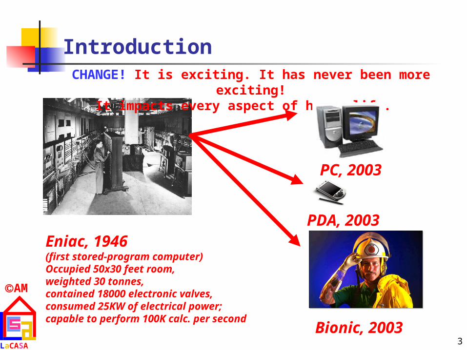
Introduction

Eniac, 1946 (first stored-program computer)Occupied 50x30 feet room, weighted 30 tonnes, contained 18000 electronic valves, consumed 25KW of electrical power;capable to perform 100K calc. per second

CHANGE! It is exciting. It has never been more exciting!It impacts every aspect of human life.

PC, 2003

PDA, 2003

Bionic, 2003

4

AM

LaCASA

Introduction (cont’d)

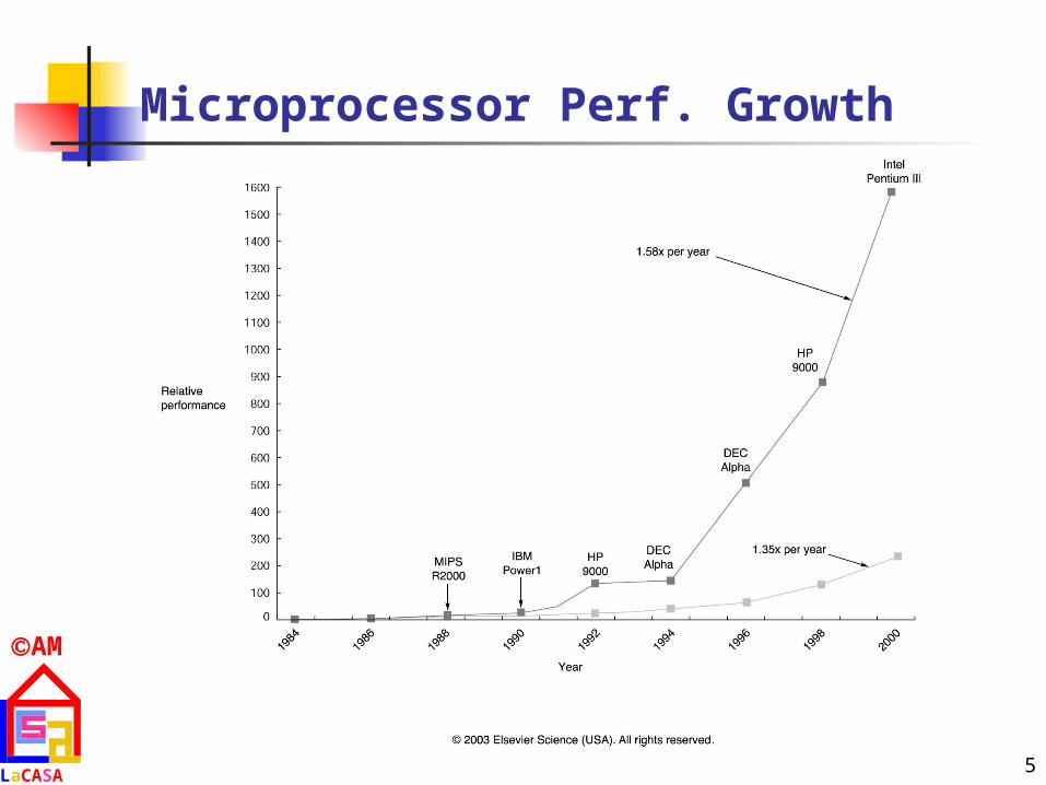
Continuous growth in performance due to advances in technology and innovations in computer design 25-30% yearly growth in performance during 1970s

Mainframes and minicomputers dominated the industry Microprocessors enabled 35%

yearly growth in performance (late 1970s) RISCs (Reduced Instruction Set Computers) enabled

50% yearly growth in performance (early 1980s)

Performance improvements through pipelining and ILP (Instruction Level Parallelism)

5

AM

LaCASA

Microprocessor Perf. Growth

6

AM

LaCASA

Effect of this Dramatic Growth

Significant enhancement of the capability available to computer user Example: your today’s PC of less than $1000 has

more performance, main memory and disk storage than $1 million computer in 1980s

Microprocessor-based computers dominate Workstations and PCs have emerged as major

products Minicomputers - replaced by servers Mainframes - replaced by multiprocessors Supercomputers - replaced by large arrays of

microprocessors

7

AM

LaCASA

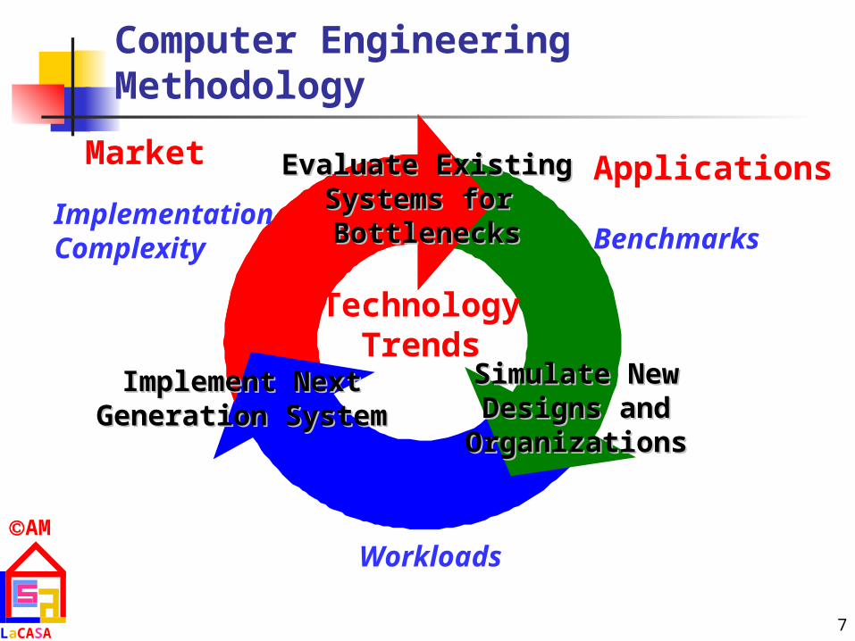
Computer Engineering Methodology

Evaluate ExistingEvaluate ExistingSystems for Systems for BottlenecksBottlenecks

Simulate NewSimulate NewDesigns andDesigns and

OrganizationsOrganizations

Implement NextImplement NextGeneration SystemGeneration System

TechnologyTrends

Benchmarks

Workloads

ImplementationComplexity

ApplicationsMarket

8

AM

LaCASA

Changing Face of Computing

In the 1960s mainframes roamed the planet Very expensive, operators oversaw operations Applications: business data processing, large scale

scientific computing In the 1970s, minicomputers emerged

Less expensive, time sharing In the 1990s, Internet and WWW, handheld devices

(PDA), high-performance consumer electronics for video games set-top boxes have emerged

Dramatic changes have led to 3 different computing markets Desktop computing, Servers, Embedded Computers

9

AM

LaCASA

Desktop Computing

Spans low-end (<$1K) to high-end ($10K) systems

Optimize price-performance Performance measured in the number of

calculations and graphic operations Price is what matters to customers

Arena where the newest highest-performance processors appear

Market force: clock rate appears as the direct measure of performance

10

AM

LaCASA

Servers

Provide more reliable file and computing services (Web servers)

Key requirements Availability – effectively provide service

24/7/365 (Yahoo!, Google, eBay) Reliability – never fails Scalability – server systems grow over time,

so the ability to scale up the computing capacity is crucial

Performance – transactions per minute

11

AM

LaCASA

Embedded Computers

Computers as parts of other devices where their presence is not obviously visible E.g., home appliances, printers, smart cards, cell

phones, palmtops Wide range of processing power and cost

$1 (8-bit, 16-bit processors), $10 (32-bit capable to execute 50M instructions per second), $100-200 (high-end video games and network switches)

Requirements Real-time performance requirement (e.g., time to

process a video frame is limited) Minimize memory requirements, power

12

AM

LaCASA

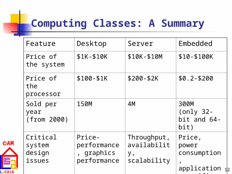
Computing Classes: A Summary

Feature Desktop Server Embedded

Price of the system

$1K-$10K $10K-$10M $10-$100K

Price of the processor

$100-$1K $200-$2K $0.2-$200

Sold per year(from 2000)

150M 4M 300M(only 32-bit and 64-bit)

Critical system design issues

Price-performance, graphics performance

Throughput, availability, scalability

Price, power consumption, application-specific performance

13

AM

LaCASA

Task of Computer Designer

“Determine what attributes are important for a new machine; then design a machine to maximize performance while staying within cost constraints.”

Aspects of this task instruction set design functional organization logic design and implementation

(IC design, packaging, power, cooling...)

14

AM

LaCASA

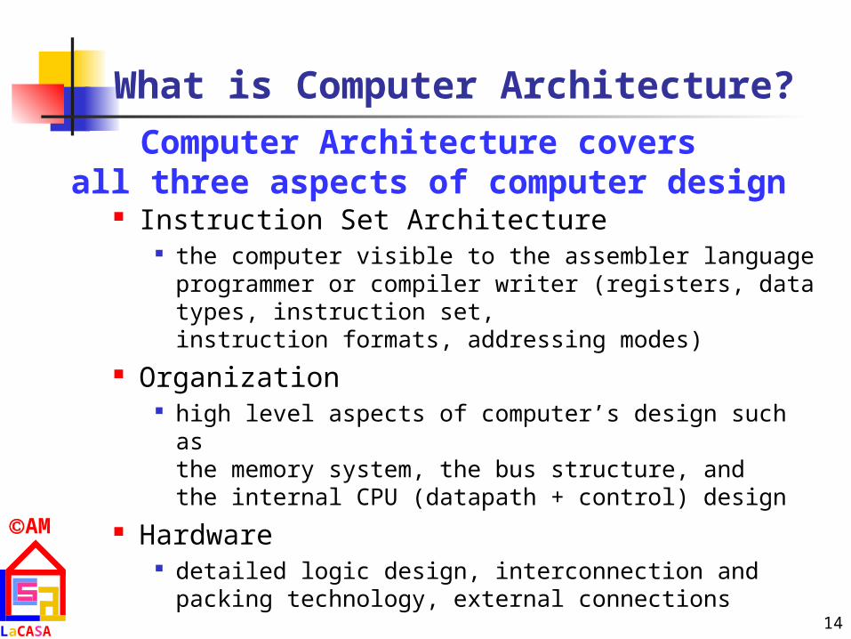
What is Computer Architecture?

Instruction Set Architecture the computer visible to the assembler language programmer

or compiler writer (registers, data types, instruction set, instruction formats, addressing modes)

Organization high level aspects of computer’s design such as

the memory system, the bus structure, and the internal CPU (datapath + control) design

Hardware detailed logic design, interconnection and packing

technology, external connections

Computer Architecture covers all three aspects of computer design

15

AM

LaCASA

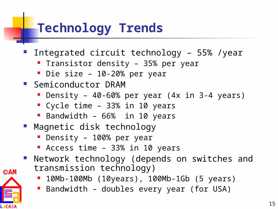
Technology Trends

Integrated circuit technology – 55% /year Transistor density – 35% per year Die size – 10-20% per year

Semiconductor DRAM Density – 40-60% per year (4x in 3-4 years) Cycle time – 33% in 10 years Bandwidth – 66% in 10 years

Magnetic disk technology Density – 100% per year Access time – 33% in 10 years

Network technology (depends on switches and transmission technology)

10Mb-100Mb (10years), 100Mb-1Gb (5 years) Bandwidth – doubles every year (for USA)

16

AM

LaCASA

Processor and Memory Capacity

MOORE’s Law 2X transistors per chip,every 1.5 years

Year Size Cycle time------------------------------------

1980 64 Kb 250 ns

1983 256 Kb 220 ns

1986 1 Mb 190 ns

1989 4 Mb 165 ns

1992 16 Mb 145 ns

1996 64 Mb 120 ns

2000 256 Mb 100 ns

2002 1 Gb ?? ns

DRAM Chip Capacity/Cycle time

Reuters, Monday 11 June 2001:Intel engineers have designed and manufactured the world’s smallest and fastest transistor in size of 0.02 microns in size. This will open the way for microprocessors of 1 billion transistors, running at 20 GHz by 2007.

Intel 4004,2300tr Intel P4 – 55M tr

Intel McKinley – 221M tr.

17

AM

LaCASA

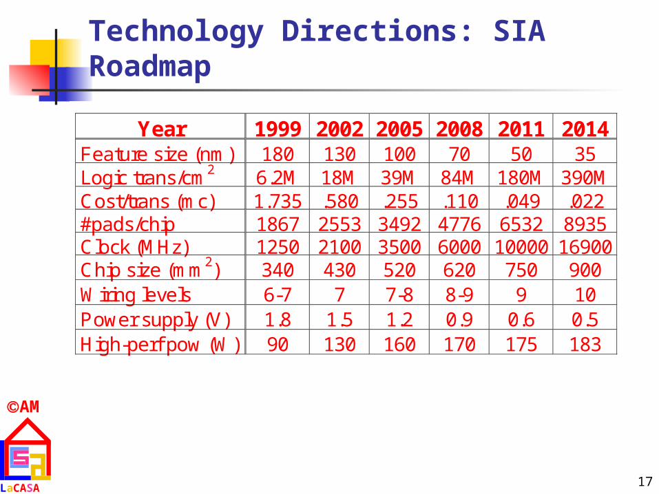
Technology Directions: SIA Roadmap

Year 1999 2002 2005 2008 2011 2014 Feature size (nm) 180 130 100 70 50 35 Logic trans/cm2 6.2M 18M 39M 84M 180M 390M Cost/trans (mc) 1.735 .580 .255 .110 .049 .022 #pads/chip 1867 2553 3492 4776 6532 8935 Clock (MHz) 1250 2100 3500 6000 10000 16900 Chip size (mm2) 340 430 520 620 750 900 Wiring levels 6-7 7 7-8 8-9 9 10 Power supply (V) 1.8 1.5 1.2 0.9 0.6 0.5 High-perf pow (W) 90 130 160 170 175 183

18

AM

LaCASA

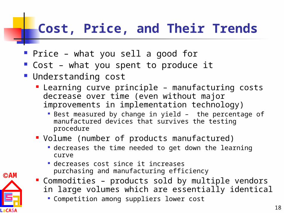
Cost, Price, and Their Trends

Price – what you sell a good for Cost – what you spent to produce it Understanding cost

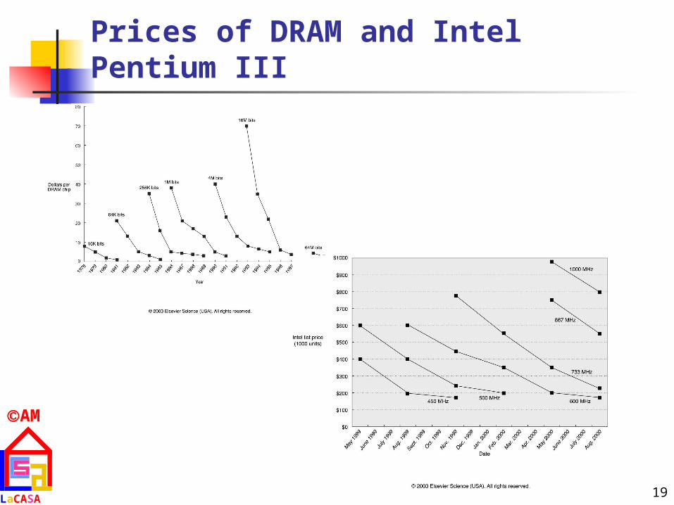
Learning curve principle – manufacturing costs decrease over time (even without major improvements in implementation technology)

Best measured by change in yield – the percentage of manufactured devices that survives the testing procedure

Volume (number of products manufactured) decreases the time needed to get down the learning curve decreases cost since it increases

purchasing and manufacturing efficiency Commodities – products sold by multiple vendors in

large volumes which are essentially identical Competition among suppliers lower cost

19

AM

LaCASA

Prices of DRAM and Intel Pentium III

20

AM

LaCASA

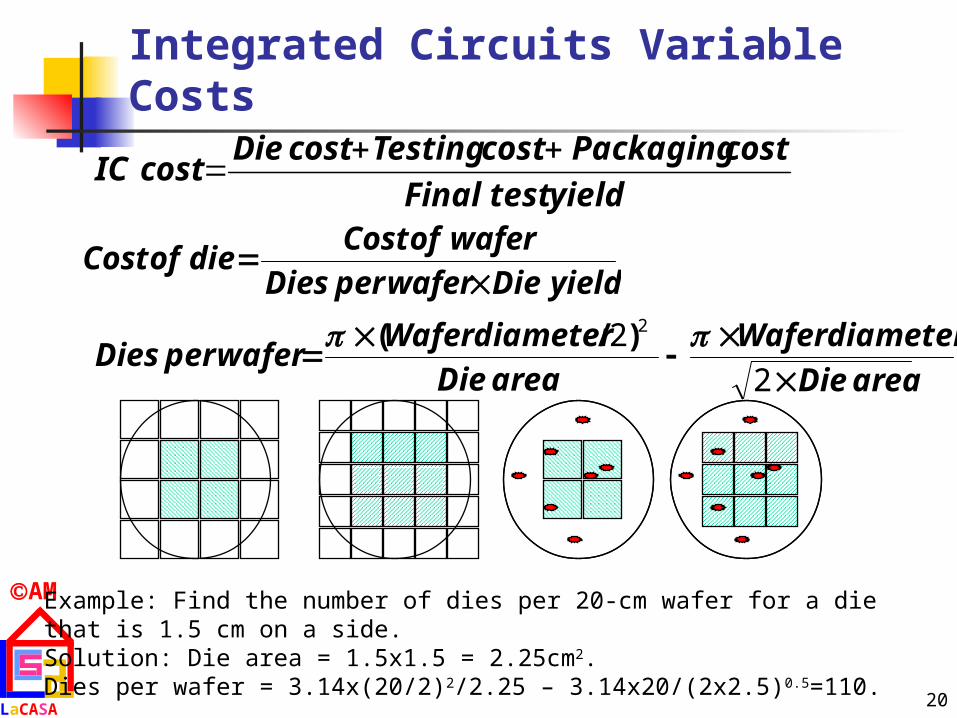
Integrated Circuits Variable Costs

yieldtestFinal

costPackagingcostTestingcostDiecostIC

yieldDiewaferperDies

waferofCostdieofCost

areaDie

diameterWafer

areaDie

diameterWaferwaferperDies

2

2 2 )/(

Example: Find the number of dies per 20-cm wafer for a die that is 1.5 cm on a side.Solution: Die area = 1.5x1.5 = 2.25cm2. Dies per wafer = 3.14x(20/2)2/2.25 – 3.14x20/(2x2.5)0.5=110.

21

AM

LaCASA

Integrated Circuits Cost (cont’d)

areaDieareaunitperDefects

yieldWaferyieldDie 1

• What is the fraction of good dies on a wafer – die yield• Empirical model

• defects are randomly distributed over the wafer• yield is inversely proportional to the complexity of the

fabrication process

• Wafer yield accounts for wafers that are completely bad

(no need to test them); We assume the wafer yield is 100%

• Defects per unit area: typically 0.4 – 0.8 per cm2 corresponds to the number of masking levels;

for today’s CMOS, a good estimate is =4.0

22

AM

LaCASA

Integrated Circuits Cost (cont’d)

areaDieareaunitperDefects

yieldWaferyieldDie 1

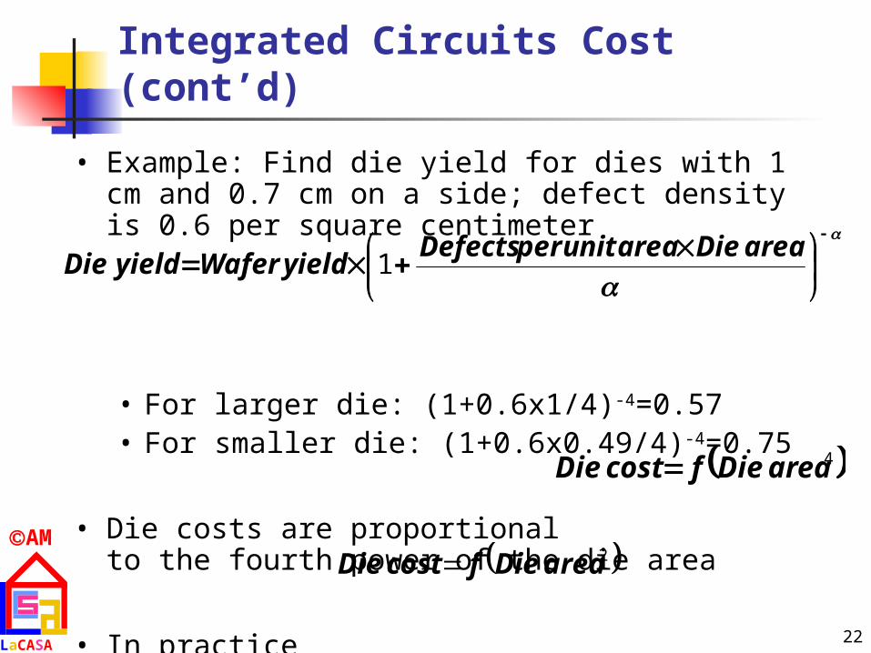
• Example: Find die yield for dies with 1 cm and 0.7 cm on a side; defect density is 0.6 per square centimeter

• For larger die: (1+0.6x1/4)-4=0.57• For smaller die: (1+0.6x0.49/4)-4=0.75

• Die costs are proportional to the fourth power of the die area

• In practice

4areaDiefcostDie

2areaDiefcostDie

23

AM

LaCASA

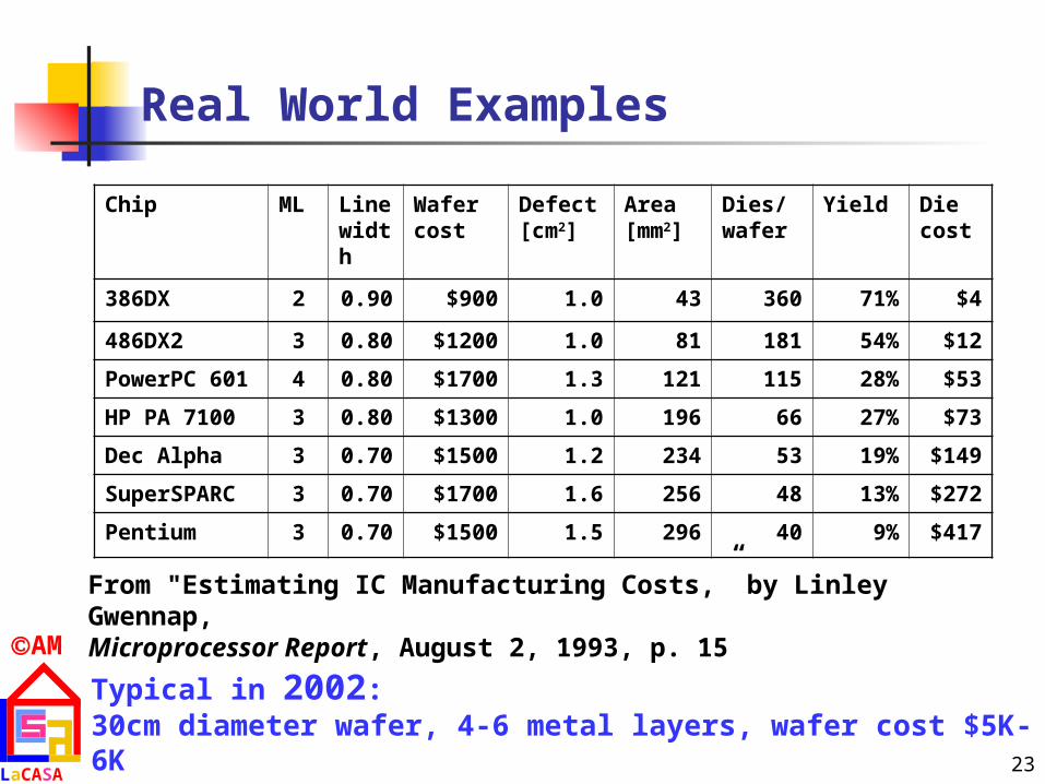
Real World Examples

Chip ML Linewidth

Wafer cost

Defect [cm2]

Area [mm2]

Dies/wafer

Yield Die cost

386DX 2 0.90 $900 1.0 43 360 71% $4

486DX2 3 0.80 $1200 1.0 81 181 54% $12

PowerPC 601 4 0.80 $1700 1.3 121 115 28% $53

HP PA 7100 3 0.80 $1300 1.0 196 66 27% $73

Dec Alpha 3 0.70 $1500 1.2 234 53 19% $149

SuperSPARC 3 0.70 $1700 1.6 256 48 13% $272

Pentium 3 0.70 $1500 1.5 296 40 9% $417

From "Estimating IC Manufacturing Costs,” by Linley Gwennap, Microprocessor Report, August 2, 1993, p. 15

Typical in 2002: 30cm diameter wafer, 4-6 metal layers, wafer cost $5K-6K

24

AM

LaCASA

Things to Remember

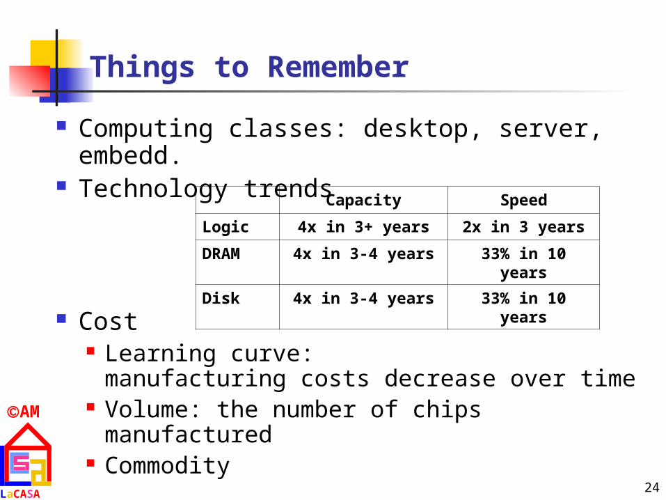
Computing classes: desktop, server, embedd. Technology trends

Cost Learning curve:

manufacturing costs decrease over time Volume: the number of chips manufactured Commodity

Capacity Speed

Logic 4x in 3+ years 2x in 3 years

DRAM 4x in 3-4 years 33% in 10 years

Disk 4x in 3-4 years 33% in 10 years

25

AM

LaCASA

Things to Remember (cont’d)

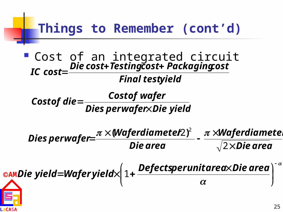
Cost of an integrated circuit

yieldtestFinal

costPackagingcostTestingcostDiecostIC

yieldDiewaferperDies

waferofCostdieofCost

areaDie

diameterWafer

areaDie

diameterWaferwaferperDies

2

2 2 )/(

areaDieareaunitperDefects

yieldWaferyieldDie 1

26

AM

LaCASA

Cost-Performance

Purchasing perspective: from a collection of machines, choose one which has best performance? least cost? best performance/cost?

Computer designer perspective: faced with design options, select one which has best performance improvement? least cost? best performance/cost?

Both require: basis for comparison and metric for evaluation

27

AM

LaCASA

Two “notions” of performance

Which computer has better performance? User: one which runs a program in less time Computer centre manager:

one which completes more jobs in a given time Users are interested in reducing

Response time or Execution time the time between the start and

the completion of an event Managers are interested in increasing

Throughput or Bandwidth total amount of work done in a given time

28

AM

LaCASA

An Example

Which has higher performance? Time to deliver 1 passenger?

Concord is 6.5/3 = 2.2 times faster (120%) Time to deliver 400 passengers?

Boeing is 72/44 = 1.6 times faster (60%)

Plane DC to Paris[hour]

Top Speed[mph]

Passe-ngers

Throughput[p/h]

Boeing 747 6.5 610 470 72 (=470/6.5)

Concorde 3 1350 132 44 (=132/3)

29

AM

LaCASA

Definition of Performance

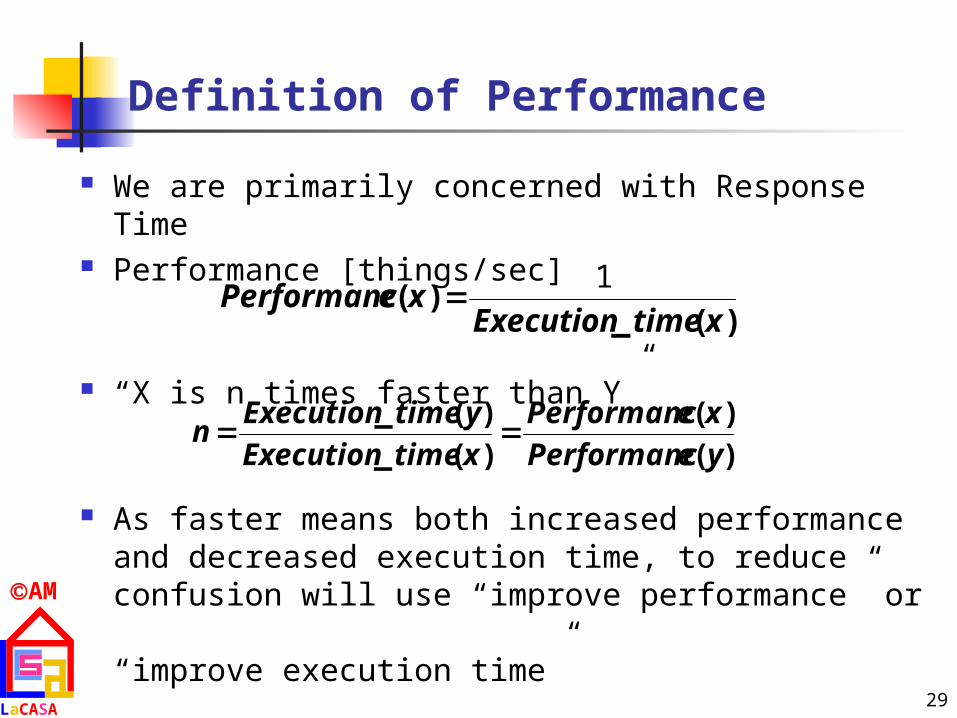
We are primarily concerned with Response Time Performance [things/sec]

“X is n times faster than Y”

As faster means both increased performance and decreased execution time, to reduce confusion will use “improve performance” or “improve execution time”

)(_)(

xtimeExecutionxePerformanc

1

)(

)(

)(_

)(_

yePerformanc

xePerformanc

xtimeExecution

ytimeExecutionn

30

AM

LaCASA

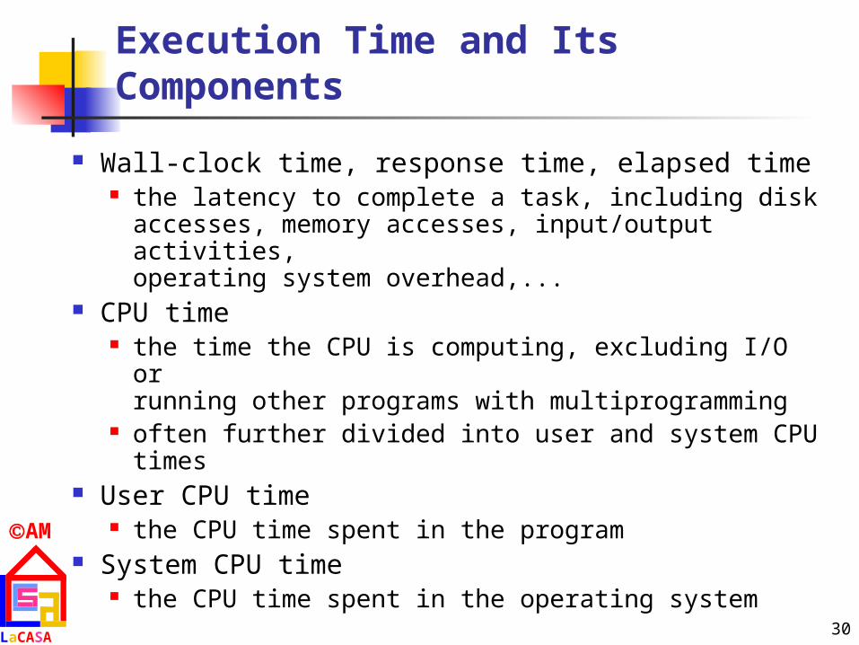
Execution Time and Its Components

Wall-clock time, response time, elapsed time the latency to complete a task, including disk

accesses, memory accesses, input/output activities, operating system overhead,...

CPU time the time the CPU is computing, excluding I/O or

running other programs with multiprogramming often further divided into user and system CPU times

User CPU time the CPU time spent in the program

System CPU time the CPU time spent in the operating system

31

AM

LaCASA

UNIX time command

90.7u 12.9s 2:39 65% 90.7 - seconds of user CPU time 12.9 - seconds of system CPU time 2:39 - elapsed time (159 seconds) 65% - percentage of elapsed time that is CPU

time(90.7 + 12.9)/159

32

AM

LaCASA

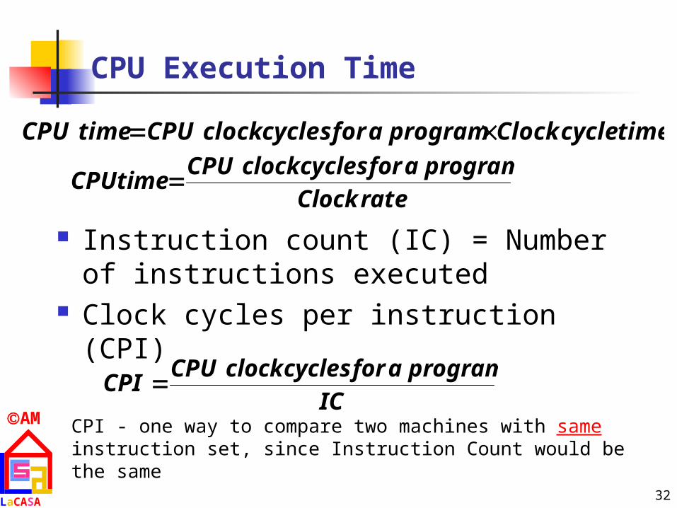
CPU Execution Time

Instruction count (IC) = Number of instructions executed

Clock cycles per instruction (CPI)

timecycleClockprogramaforcyclesclockCPUtimeCPU

rateClock

programaforcyclesclockCPUCPUtime

IC

programaforcyclesclockCPUCPI

CPI - one way to compare two machines with same instruction set, since Instruction Count would be the same

33

AM

LaCASA

CPU Execution Time (cont’d)

timecycleClockCPIICtimeCPU

rateClock

CPIICtimeCPU

IC CPI Clock rate

Program X

Compiler X (X)

ISA X X

Organisation X X

Technology X

Program

Seconds

cycleClock

Seconds

nInstructio

cyclesClock

Program

nsInstructiotimeCPU

34

AM

LaCASA

How to Calculate 3 Components?

Clock Cycle Time in specification of computer

(Clock Rate in advertisements) Instruction count

Count instructions in loop of small program Use simulator to count instructions Hardware counter in special register (Pentium II)

CPI Calculate:

Execution Time / Clock cycle time / Instruction Count Hardware counter in special register (Pentium II)

35

AM

LaCASA

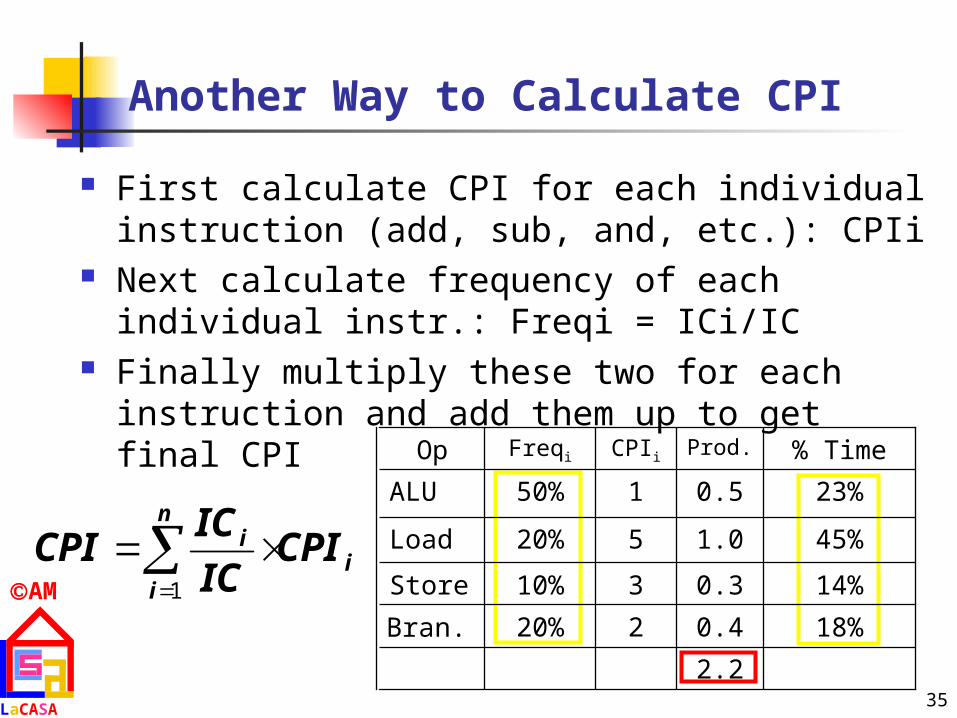
Another Way to Calculate CPI

First calculate CPI for each individual instruction (add, sub, and, etc.): CPIi

Next calculate frequency of each individual instr.: Freqi = ICi/IC

Finally multiply these two for each instruction and add them up to get final CPI

2.2

18%

14%

45%

23%

% Time

0.4220%Bran.

0.3310%Store

1.0520%Load

0.5150%ALU

Prod.CPIiFreqiOp

i

n

i

i CPIIC

ICCPI

1

36

AM

LaCASA

Choosing Programs to Evaluate Per.

Ideally run typical programs with typical input before purchase, or before even build machine Engineer uses compiler, spreadsheet Author uses word processor, drawing program,

compression software Workload – mixture of programs and OS commands

that users run on a machine Few can do this

Don’t have access to machine to “benchmark” before purchase

Don’t know workload in future

37

AM

LaCASA

Benchmarks

Different types of benchmarks Real programs (Ex. MSWord, Excel, Photoshop,...) Kernels - small pieces from real programs (Linpack,...) Toy Benchmarks - short, easy to type and run

(Sieve of Erathosthenes, Quicksort, Puzzle,...) Synthetic benchmarks - code that matches frequency

of key instructions and operations to real programs (Whetstone, Dhrystone)

Need industry standards so that different processors can be fairly compared

Companies exist that create these benchmarks: “typical” code used to evaluate systems

38

AM

LaCASA

Benchmark Suites

SPEC - Standard Performance Evaluation Corporation (www.spec.org) originally focusing on CPU performance

SPEC89|92|95, SPEC CPU2000 (11 Int + 13 FP) graphics benchmarks: SPECviewperf, SPECapc server benchmark: SPECSFS, SPECWEB

PC benchmarks (Winbench 99, Business Winstone 99, High-end Winstone 99, CC Winstone 99) (www.zdnet.com/etestinglabs/filters/benchmarks)

Transaction processing benchmarks (www.tpc.org) Embedded benchmarks (www.eembc.org)

39

AM

LaCASA

Comparing and Summarising Per.

An Example

What we can learn from these statements? We know nothing about

relative performance of computers A, B, C! One approach to summarise relative performance:

use total execution times of programs

Program Com. A Com. B Com. C

P1 (sec) 1 10 20

P2 (sec) 1000 100 20

Total (sec) 1001 110 40

– A is 20 times faster than C for program P1– C is 50 times faster than A for program P2– B is 2 times faster than C for program P1– C is 5 times faster than B for program P2

40

AM

LaCASA

Comparing and Sum. Per. (cont’d)

Arithmetic mean (AM) or weighted AM to track time

Harmonic mean or weighted harmonic mean of rates tracks execution time

Normalized execution time to a reference machine do not take arithmetic mean of normalized execution

times, use geometric mean

n

iiTime

n 0

1

n

iii Timew

0

Timei – execution time for ith programwi – frequency of that program in workload

iin

i i

TimeRate

Rate

n 1,

1

0

n

i i

i

Ratew

0

1

n

iiratioExTime

n

1

1 Problem: GM rewards equally the following improvements:Program A: from 2s to 1s, andProgram B: from 2000s to 1000s

41

AM

LaCASA

Quantitative Principles of Design

Where to spend time making improvements? Make the Common Case Fast Most important principle of computer design:

Spend your time on improvements where those improvements will do the most good

Example Instruction A represents 5% of execution Instruction B represents 20% of execution Even if you can drive the time for A to 0, the CPU will only be

5% faster Key questions

What the frequent case is? How much performance can be improved by making

that case faster?

42

AM

LaCASA

Amdahl’s Law

Suppose that we make an enhancement to a machine that will improve its performance; Speedup is ratio:

Amdahl’s Law states that the performance improvement that can be gained by a particular enhancement is limited by the amount of time that enhancement can be used

tenhancemenusingtaskentireforExTime

tenhancemenwithouttaskentireforExTimeSpeedup

tenhancemenwithouttaskentireforePerformanc

tenhancemenusingtaskentireforePerformancSpeedup

43

AM

LaCASA

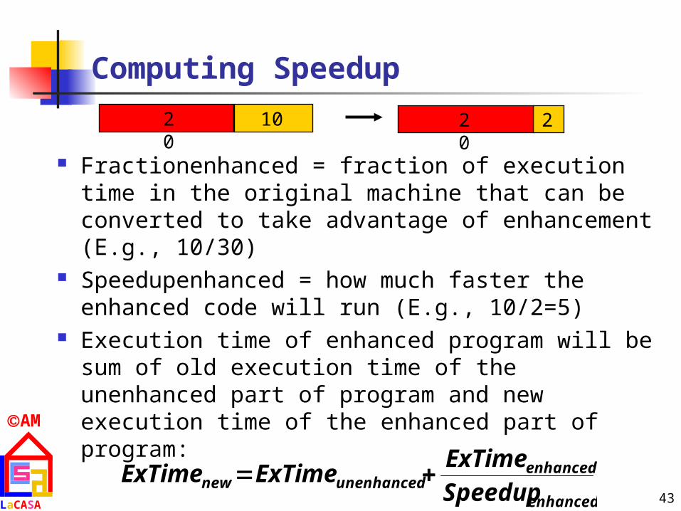
Computing Speedup

Fractionenhanced = fraction of execution time in the original machine that can be converted to take advantage of enhancement (E.g., 10/30)

Speedupenhanced = how much faster the enhanced code will run (E.g., 10/2=5)

Execution time of enhanced program will be sum of old execution time of the unenhanced part of program and new execution time of the enhanced part of program:

enhanced

enhancedunenhancednew Speedup

ExTimeExTimeExTime

20 10 20 2

44

AM

LaCASA

Computing Speedup (cont’d)

Enhanced part of program is Fractionenhanced, so times are:

Factor out Timeold and divide by Speedupenhanced:

Overall speedup is ratio of Timeold to Timenew:

enhancedoldunenhanced FractionExTimeExTime 1

enhancedoldenhanced FractionExTimeExTime

enhanced

enhancedenhancedoldnew Speedup

FractionFractionExTimeExTime 1

enhanced

enhancedenhanced Speedup

FractionFraction

Speedup

1

1

45

AM

LaCASA

An Example

Enhancement runs 10 times faster and it affects 40% of the execution time

Fractionenhanced = 0.40 Speedupenhanced = 10 Speedupoverall = ?

561640

1

1040

401

1.

...

Speedup

46

AM

LaCASA

“Law of Diminishing Returns”

Suppose that same piece of code can now be enhanced another 10 times

Fractionenhanced = 0.04/(0.60 + 0.04) = 0.0625

Speedupenhanced = 10

059.1

1006.0

94.0

1

1

1

overall

enhanced

enhancedenhanced

overall

Speedup

SpeedupFraction

FractionSpeedup

47

AM

LaCASA

Using CPU Performance Equations

Example #1: consider 2 alternatives for conditional branch instructions

CPU A: a condition code (CC) is set by a compare instruction and followed by a branch instruction that test CC

CPU B: a compare is included in the branch Assumptions:

on both CPUs, the conditional branch takes 2 clock cycles all other instructions take 1 clock cycle on CPU A, 20% of all instructions executed are cond. branches;

since every branch needs a compare, another 20% are compares because CPU A does not have a compare included in the branch,

assume its clock cycle time is 1.25 times faster than that of CPU B Which CPU is faster? Answer the question when CPU A clock cycle time is only 1.1

times faster than that of CPU B

48

AM

LaCASA

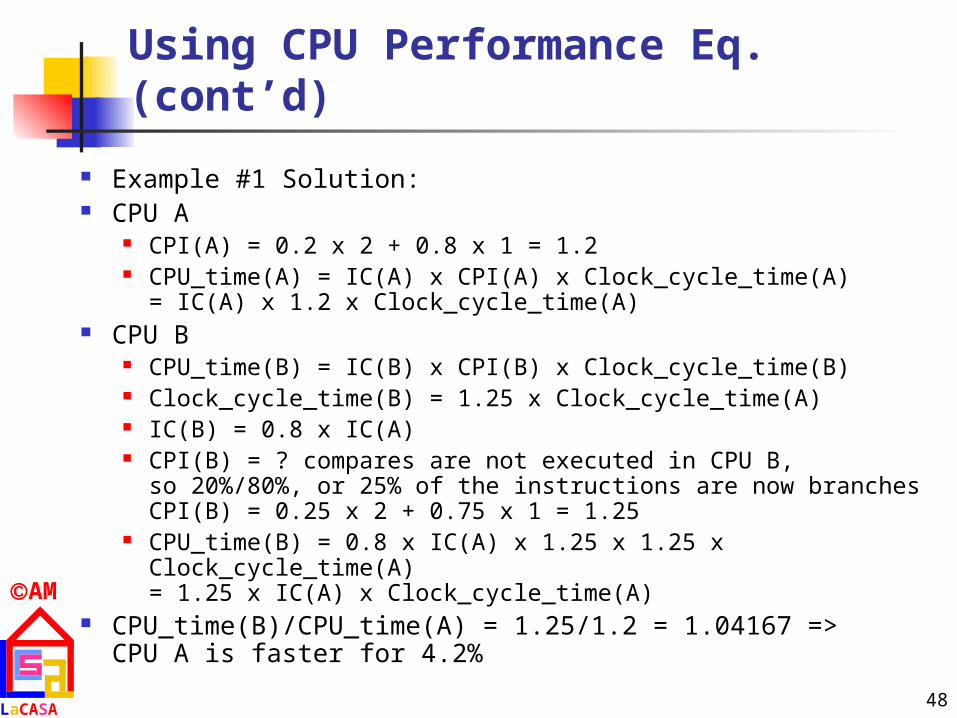
Using CPU Performance Eq. (cont’d)

Example #1 Solution: CPU A

CPI(A) = 0.2 x 2 + 0.8 x 1 = 1.2 CPU_time(A) = IC(A) x CPI(A) x Clock_cycle_time(A)

= IC(A) x 1.2 x Clock_cycle_time(A) CPU B

CPU_time(B) = IC(B) x CPI(B) x Clock_cycle_time(B) Clock_cycle_time(B) = 1.25 x Clock_cycle_time(A) IC(B) = 0.8 x IC(A) CPI(B) = ? compares are not executed in CPU B,

so 20%/80%, or 25% of the instructions are now branchesCPI(B) = 0.25 x 2 + 0.75 x 1 = 1.25

CPU_time(B) = 0.8 x IC(A) x 1.25 x 1.25 x Clock_cycle_time(A)= 1.25 x IC(A) x Clock_cycle_time(A)

CPU_time(B)/CPU_time(A) = 1.25/1.2 = 1.04167 =>CPU A is faster for 4.2%

49

AM

LaCASA

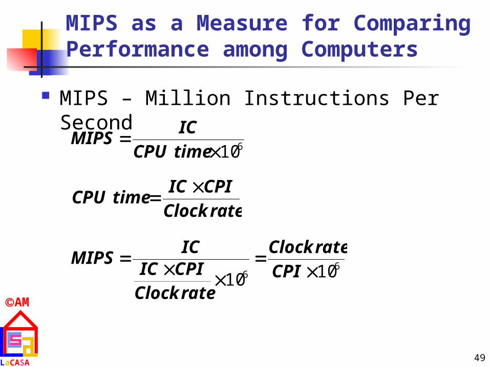
MIPS as a Measure for Comparing Performance among Computers

MIPS – Million Instructions Per Second

610

timeCPU

ICMIPS

rateClock

CPIICtimeCPU

66 1010

CPI

rateClock

rateClockCPIICIC

MIPS

50

AM

LaCASA

MIPS as a Measure for Comparing Performance among Computers (cont’d)

Problems with using MIPS as a measure for comparison MIPS is dependent on the instruction set,

making it difficult to compare MIPS of computers with different instruction sets

MIPS varies between programs on the same computer

Most importantly, MIPS can vary inversely to performance

Example: MIPS rating of a machine with optional FP hardware

Example: Code optimization

51

AM

LaCASA

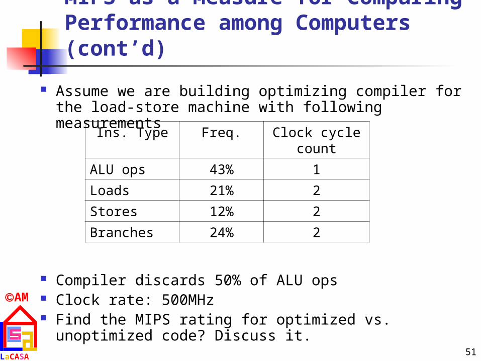
MIPS as a Measure for Comparing Performance among Computers (cont’d)

Assume we are building optimizing compiler for the load-store machine with following measurements

Compiler discards 50% of ALU ops Clock rate: 500MHz Find the MIPS rating for optimized vs. unoptimized

code? Discuss it.

Ins. Type Freq. Clock cycle count

ALU ops 43% 1

Loads 21% 2

Stores 12% 2

Branches 24% 2

52

AM

LaCASA

MIPS as a Measure for Comparing Performance among Computers (cont’d)

Unoptimized CPI(u) = 0.43 x 1 + 0.57 x 2 = 1.57 MIPS(u) = 500MHz/(1.57 x 106)=318.5 CPU_time(u) = IC(u) x CPI(u) x Clock_cycle_time

= IC(u) x 1.57 x 2 x 10-9 = 3.14 x 10-9 x IC(u) Optimized

CPI(o) = [(0.43/2) x 1 + 0.57 x 2]/(1 – 0.43/2) = 1.73 MIPS(o) = 500MHz/(1.73 x 106)=289.0 CPU_time(o) = IC(o) x CPI(o) x Clock_cycle_time

= 0.785 x IC(u) x 1.73 x 2 x 10-9 = 2.72 x 10-9 x IC(u)

53

AM

LaCASA

Things to Remember

Execution, Latency, Res. time: time to run the task

Throughput, bandwidth: tasks per day, hour, sec

User Time time user needs to wait for program to execute:

depends heavily on how OS switches between tasks CPU Time

time spent executing a single program: depends solely on design of processor (datapath, pipelining effectiveness, caches, etc.)

54

AM

LaCASA

Things to Remember (cont’d)

Benchmarks: good products created when have good benchmarks

CPI Law

Amdahl’s Law

enhanced

enhancedenhanced Speedup

FractionFraction

Speedup

1

1

Program

Seconds

cycleClock

Seconds

nInstructio

cyclesClock

Program

nsInstructiotimeCPU

55

AM

LaCASA

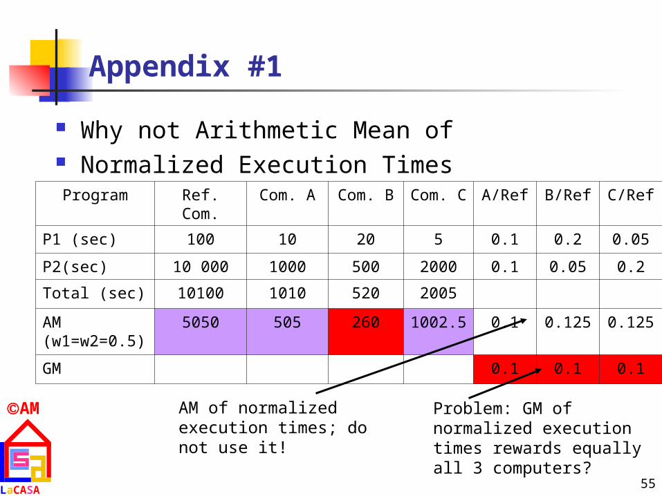
Appendix #1

Why not Arithmetic Mean of Normalized Execution Times

Program Ref. Com. Com. A Com. B Com. C A/Ref B/Ref C/Ref

P1 (sec) 100 10 20 5 0.1 0.2 0.05

P2(sec) 10 000 1000 500 2000 0.1 0.05 0.2

Total (sec) 10100 1010 520 2005

AM (w1=w2=0.5)

5050 505 260 1002.5 0.1 0.125 0.125

GM 0.1 0.1 0.1

Problem: GM of normalized execution times rewards equally all 3 computers?

AM of normalized execution times; do not use it!