Embed Size (px)
Citation preview

University of Kentucky University of Kentucky
UKnowledge UKnowledge
Theses and Dissertations--Computer Science Computer Science
2016
CP-nets: From Theory to Practice CP-nets: From Theory to Practice
Thomas E. Allen University of Kentucky, [email protected] Digital Object Identifier: http://dx.doi.org/10.13023/ETD.2016.131
Right click to open a feedback form in a new tab to let us know how this document benefits you. Right click to open a feedback form in a new tab to let us know how this document benefits you.
Recommended Citation Recommended Citation Allen, Thomas E., "CP-nets: From Theory to Practice" (2016). Theses and Dissertations--Computer Science. 42. https://uknowledge.uky.edu/cs_etds/42
This Doctoral Dissertation is brought to you for free and open access by the Computer Science at UKnowledge. It has been accepted for inclusion in Theses and Dissertations--Computer Science by an authorized administrator of UKnowledge. For more information, please contact [email protected].

STUDENT AGREEMENT: STUDENT AGREEMENT:
I represent that my thesis or dissertation and abstract are my original work. Proper attribution
has been given to all outside sources. I understand that I am solely responsible for obtaining
any needed copyright permissions. I have obtained needed written permission statement(s)
from the owner(s) of each third-party copyrighted matter to be included in my work, allowing
electronic distribution (if such use is not permitted by the fair use doctrine) which will be
submitted to UKnowledge as Additional File.
I hereby grant to The University of Kentucky and its agents the irrevocable, non-exclusive, and
royalty-free license to archive and make accessible my work in whole or in part in all forms of
media, now or hereafter known. I agree that the document mentioned above may be made
available immediately for worldwide access unless an embargo applies.
I retain all other ownership rights to the copyright of my work. I also retain the right to use in
future works (such as articles or books) all or part of my work. I understand that I am free to
register the copyright to my work.
REVIEW, APPROVAL AND ACCEPTANCE REVIEW, APPROVAL AND ACCEPTANCE
The document mentioned above has been reviewed and accepted by the student’s advisor, on
behalf of the advisory committee, and by the Director of Graduate Studies (DGS), on behalf of
the program; we verify that this is the final, approved version of the student’s thesis including all
changes required by the advisory committee. The undersigned agree to abide by the statements
above.
Thomas E. Allen, Student
Dr. Judy Goldsmith, Major Professor
Dr. Mirosław Truszczyński, Director of Graduate Studies

CP-NETS: FROM THEORY TO PRACTICE
DISSERTATION
A dissertation submitted in partialfulfillment of the requirements for thedegree of Doctor of Philosophy in the
College of Engineering at theUniversity of Kentucky
By
Thomas E. Allen
Lexington, Kentucky
Director: Dr. Judy Goldsmith, Professor of Computer Science
Lexington, Kentucky
2016
Copyright c© Thomas E. Allen 2016

ABSTRACT OF DISSERTATION
CP-NETS: FROM THEORY TO PRACTICE
Conditional preference networks (CP-nets) exploit the power of ceteris paribus rules torepresent preferences over combinatorial decision domains compactly. CP-nets have muchappeal. However, their study has not yet advanced sufficiently for their widespread usein real-world applications. Known algorithms for deciding dominance—whether one out-come is better than another with respect to a CP-net—require exponential time. Data forCP-nets are difficult to obtain: human subjects data over combinatorial domains are notreadily available, and earlier work on random generation is also problematic. Also, muchof the research on CP-nets makes strong, often unrealistic assumptions, such as that deci-sion variables must be binary or that only strict preferences are permitted. In this thesis,I address such limitations to make CP-nets more useful. I show how: to generate CP-netsuniformly randomly; to limit search depth in dominance testing given expectations aboutsets of CP-nets; and to use local search for learning restricted classes of CP-nets fromchoice data.
KEYWORDS: artificial intelligence, combinatorial preferences, decision making, appli-cations of local search, conditional preference networks
Author’s signature: Thomas E. Allen
Date: April 29, 2016

CP-NETS: FROM THEORY TO PRACTICE
By
Thomas E. Allen
Director of Dissertation: Judy Goldsmith
Director of Graduate Studies: Mirosław Truszczynski
Date: April 29, 2016

To Susan, Luke, and Seth

ACKNOWLEDGMENTS
Five years ago, after a number of years serving in a different profession, I returned to grad-
uate school to pursue a Ph.D. in computer science. I recognize how fortunate I am to have
had such an opportunity. Many people helped make this possible—more than I can pos-
sibly list here—and I am grateful for their encouragement and support along the way. In
particular, I am grateful for my advisor, Dr. Judy Goldsmith. Shortly after I began planning
to pursue graduate studies, I came across some of her journal articles on computational
decision making. We met for lunch at the Mellow Mushroom restaurant in Lexington. I
rambled on about my “crazy idea” of pursing a career in academia, and she encouraged me
to take the GRE and apply to Ph.D. programs. This was the start of a mentoring process
that has continued up to the present time. I am grateful for her extraordinary support and
friendship throughout this process. I am thankful also to Dr. Raphael Finkel, the Director
of Graduate Studies for the Department of Computer Science at the time. I had submit-
ted all the pieces of my application for admission except the essay explaining my goals
in pursuing a Ph.D., which at that point were somewhat less than clear. He took the un-
usual step of contacting me by telephone and admitting me to the program after a lengthy
conversation. I am grateful to the members of my Doctoral Advisory Committee. In addi-
tion to Dr. Goldsmith, who served as the director, that committee consisted of Drs. Mirek
Truszczynski, Victor Marek, Clyde Holsapple, and Paul Eakin. Dr. Truszczynski, in addi-
tion to serving as our current Director of Graduate Studies, suggested the journal in which
we found the article with the encoding for directed acyclic graphs that proved foundational
to the method of generating CP-nets that I describe in Chapter 4; I also had the privilege
of taking Dr. Truszczynski’s special topics course in social networks. From Dr. Marek, I
took two courses, one on databases and another on Constraint Satisfaction Programming.
The latter introduced me to the use of SAT solvers, which ultimately led to the DT-SAT
iii

reduction that I describe in Section 5.6.2. From Dr. Holsapple, I took a course on Deci-
sion Support Systems that helped motivate some of my interest in practical applications for
CP-nets. Dr. Holsapple also provided constructive feedback on an earlier draft of this dis-
sertation that resulted in many improvements. I am grateful also to Dr. Eakin, the external
member of the committee, for his time and effort near the end of the process.
I am especially grateful to my coauthors. They perused my sometimes bewildering
early drafts, asked hard questions and helped me to expand, clarify, and in some cases cor-
rect my ideas. Some of them wrote software or revised problematic passages. Dr. Nick
Mattei of Data61 and UNSW Australia collaborated with Dr. Goldsmith and me on the
workshop paper [2] that eventually led to Chapter 4. Kayla Raines and Hayden Elizabeth
Justice, both of whom were undergraduate students at the time, assisted with a later version
of that work that was accepted for publication at the prestigious AAAI-16 conference [5].
Cory Siler, another undergraduate student, collaborated with Dr. Goldsmith and me on an
earlier draft of what is now Chapter 6. Cory also contributed much of the programming for
the experiment summarized in 6.2, as well as the implementation of Lehmer codes men-
tioned in Section 4.2. Dr. Joshua T. Guerin of the University of Tennessee Martin kindly al-
lowed me to assist in rewriting a chapter of his dissertation for a conference publication that
was ultimately accepted for presentation at ADT 2013 [47]. That was my first academic
publication and also my introduction to conditional preference networks. I am grateful to
Dr. Francesca Rossi, whom we visited at the University of Padua in Italy in November
2013, and to her students, in particular Cristina Cornelio, who introduced us to PCP-nets;
they provided invaluable feedback on our work. In addition, Drs. Rossi, Goldsmith, and I
later collaborated on a CP-nets tutorial at AAAI-16. I am grateful to Dr. Mike Regenwetter
of the University of Illinois Urbana-Champaign, and to his students, in particular Dr. Anna
Popova, Muye Chen, and Chistopher Zwilling. Drs. Regenwetter, Goldsmith, and Rossi
and their labs have collaborated on a human subjects study involving CP-nets [3] that has
been nearing completion for the past several years. Mike also introduced me to his col-
iv

league, Olgica Milenkovic, leading to the invitation to present my paper on CP-nets at the
Allerton Conference in 2013 [1], parts of which later found there way into Chapter 5. Five
of my papers—three conference papers [3, 5, 47] and two workshop papers [2, 4]—also
went through a referee process, occasionally more than once. Along with my coauthors I
am grateful to the anonymous reviewers for their constructive critiques.
My studies at the University of Kentucky were made possible by teaching and research
assistantships and fellowships, including a grant from the National Science Foundation
(CCF-121598), Graduate School Academic Year Fellowships in 2013–2014 and 2015–
2016, a Verizon Fellowship in Fall 2014, and the Thaddeus B. Curtz Memorial Scholarship
Award in 2012. I am also grateful to the citizens of the Commonwealth of Kentucky, where
I have lived since 2004, for their support of higher education.
I am deeply appreciative also of my family and friends for their support in this endeavor.
I still remember the considerable satisfaction of my father, Dr. T. Eugene Allen III, when he
completed his Ph.D. in political science when I was a small child. He and my mother, Ann
Lyn Allen, who was also my high school mathematics teacher, met in a statistics class in
graduate school. They instilled in me a high regard for the value of education. My siblings,
Dr. Martha Allen-Dietrich of Georgia College and State University, and Dr. Timothy E.
Allen of the University of Virginia, have also offered guidance and encouragement during
my transition into academic life. Finally, and most especially, I am grateful to Susan,
my wife, and to my sons, Luke and Seth, for letting me devote so many years to such a
challenging and transformative process. My appreciation for them is beyond words, and to
them this work is lovingly dedicated.
v

TABLE OF CONTENTS
Acknowledgments . . . . . . . . . . . . . . . . . . . . . . . . . . . . . . . . . . . . iii
Table of Contents . . . . . . . . . . . . . . . . . . . . . . . . . . . . . . . . . . . . vi
List of Tables . . . . . . . . . . . . . . . . . . . . . . . . . . . . . . . . . . . . . . viii
List of Figures . . . . . . . . . . . . . . . . . . . . . . . . . . . . . . . . . . . . . . ix
Chapter 1 Introduction . . . . . . . . . . . . . . . . . . . . . . . . . . . . . . . . 11.1 Preferences . . . . . . . . . . . . . . . . . . . . . . . . . . . . . . . . . . 2
1.1.1 Utility, Strict Preference, and Indifference . . . . . . . . . . . . . . 41.1.2 Incomparability, Incompleteness, and Missing Information . . . . . 51.1.3 Transitivity and Inconsistent Preferences . . . . . . . . . . . . . . . 61.1.4 Factored Outcomes and Ceteris Paribus Preferences . . . . . . . . . 8
1.2 Preferences over Combinatorial Domains . . . . . . . . . . . . . . . . . . 91.2.1 Non-compact Representations . . . . . . . . . . . . . . . . . . . . 101.2.2 Compact Preference Formalisms . . . . . . . . . . . . . . . . . . . 111.2.3 Common Problems in Preference Handling . . . . . . . . . . . . . 13
1.3 Conditional Preference Networks . . . . . . . . . . . . . . . . . . . . . . . 151.4 CP-nets: Challenges to Adoption . . . . . . . . . . . . . . . . . . . . . . . 18
Chapter 2 Definitions . . . . . . . . . . . . . . . . . . . . . . . . . . . . . . . . . 202.1 Ordered Sets . . . . . . . . . . . . . . . . . . . . . . . . . . . . . . . . . . 202.2 Graphs . . . . . . . . . . . . . . . . . . . . . . . . . . . . . . . . . . . . . 212.3 Outcomes . . . . . . . . . . . . . . . . . . . . . . . . . . . . . . . . . . . 252.4 Preferences and CP-nets . . . . . . . . . . . . . . . . . . . . . . . . . . . . 262.5 Commonly Used Notation and Abbreviations . . . . . . . . . . . . . . . . 33
Chapter 3 Related Work . . . . . . . . . . . . . . . . . . . . . . . . . . . . . . . 383.1 General and Restricted CP-net Models . . . . . . . . . . . . . . . . . . . . 383.2 Finding Most Preferred Outcomes . . . . . . . . . . . . . . . . . . . . . . 393.3 Checking for Consistency . . . . . . . . . . . . . . . . . . . . . . . . . . . 403.4 Reasoning with CP-nets . . . . . . . . . . . . . . . . . . . . . . . . . . . . 41
3.4.1 Dominance Testing . . . . . . . . . . . . . . . . . . . . . . . . . . 413.4.2 Ordering Queries . . . . . . . . . . . . . . . . . . . . . . . . . . . 423.4.3 Reductions and Heuristic Methods . . . . . . . . . . . . . . . . . . 43
3.5 Learning CP-nets . . . . . . . . . . . . . . . . . . . . . . . . . . . . . . . 433.6 Experiments with CP-nets . . . . . . . . . . . . . . . . . . . . . . . . . . . 463.7 Extensions to the Formalism . . . . . . . . . . . . . . . . . . . . . . . . . 47
vi

Chapter 4 Generating CP-nets Uniformly at Random . . . . . . . . . . . . . . . . 494.1 Naıve Generation, Bias, and Degeneracy . . . . . . . . . . . . . . . . . . . 504.2 Counting and Generating the CPTs . . . . . . . . . . . . . . . . . . . . . . 544.3 Encoding and Counting Dependency Graphs . . . . . . . . . . . . . . . . . 604.4 Generating CP-nets . . . . . . . . . . . . . . . . . . . . . . . . . . . . . . 664.5 Generating Outcomes and DT Problem Instances . . . . . . . . . . . . . . 744.6 Conclusion . . . . . . . . . . . . . . . . . . . . . . . . . . . . . . . . . . 75
Chapter 5 Depth-Limited Dominance Testing . . . . . . . . . . . . . . . . . . . . 765.1 Preliminaries . . . . . . . . . . . . . . . . . . . . . . . . . . . . . . . . . 775.2 Experiment 1: An Exhaustive Consideration of Tiny Cases . . . . . . . . . 815.3 Experiment 2: Sampling CP-nets and Solving DT for all Outcomes . . . . . 905.4 Experiment 3: A Consideration of Larger Instances . . . . . . . . . . . . . 955.5 Are Preferences Really Transitive? . . . . . . . . . . . . . . . . . . . . . . 995.6 Depth-Limited Dominance Testing . . . . . . . . . . . . . . . . . . . . . . 100
5.6.1 Depth-Limited DT* . . . . . . . . . . . . . . . . . . . . . . . . . . 1015.6.2 DT-SAT . . . . . . . . . . . . . . . . . . . . . . . . . . . . . . . . 102
5.7 Conclusion . . . . . . . . . . . . . . . . . . . . . . . . . . . . . . . . . . 106
Chapter 6 Local Search for Learning Tree-Shaped CP-nets . . . . . . . . . . . . . 1086.1 Background . . . . . . . . . . . . . . . . . . . . . . . . . . . . . . . . . . 1096.2 Encoding Tree-shaped CP-nets . . . . . . . . . . . . . . . . . . . . . . . . 1126.3 Evaluating a Learned Model . . . . . . . . . . . . . . . . . . . . . . . . . 1216.4 Learning via Local Search . . . . . . . . . . . . . . . . . . . . . . . . . . 1236.5 Experiments . . . . . . . . . . . . . . . . . . . . . . . . . . . . . . . . . . 1266.6 Conclusion . . . . . . . . . . . . . . . . . . . . . . . . . . . . . . . . . . 133
Chapter 7 Conclusion . . . . . . . . . . . . . . . . . . . . . . . . . . . . . . . . 134
Bibliography . . . . . . . . . . . . . . . . . . . . . . . . . . . . . . . . . . . . . . 135
Vita . . . . . . . . . . . . . . . . . . . . . . . . . . . . . . . . . . . . . . . . . . . 143
vii

LIST OF TABLES
2.1 Commonly Used Acronyms . . . . . . . . . . . . . . . . . . . . . . . . . . . . 332.2 Commonly Used Notation . . . . . . . . . . . . . . . . . . . . . . . . . . . . 34
3.1 CP-nets Characterized by Dependency Graph . . . . . . . . . . . . . . . . . . 403.2 Computational Difficulty of Dominance Testing . . . . . . . . . . . . . . . . . 423.3 Evaluation Methods for Proposed CP-net Algorithms . . . . . . . . . . . . . . 47
4.1 Values of φ2(m) and ψ2(m) for m = 0 to 5 . . . . . . . . . . . . . . . . . . . . . 564.2 Odds of Generating a Degenerate Function at Random on a Given Attempt . . . 604.3 Number of DAGs an,c with n Nodes and Bound c on Indegree . . . . . . . . . . 664.4 Number of Binary CP-nets with Complete CPTs and Unbounded Indegree . . . 704.5 Values of an,c,d for Small Values of n, c, and d . . . . . . . . . . . . . . . . . . 71
5.1 Computational Difficulty of Dominance Testing (Table 3.2 Revisited) . . . . . 795.2 Cardinalities of O2 and DT(N,O) . . . . . . . . . . . . . . . . . . . . . . . . 805.3 Number of DT Solutions Given HD and FL (n = 9; c = 1 and c = 2) . . . . . . 925.4 Number of DT Solutions Given HD and FL (n = 9; c = 3 and c = 4) . . . . . . 935.5 Mean Flipping Length Given n, c, and h (for n = 5 to 9) . . . . . . . . . . . . . 945.6 Mean Flipping Length Given n, c, and h (Binary Variables, n = 10 to 15) . . . . 975.7 Mean Flipping Length Given n, c, and h (Multivalued Variables d = 3) . . . . . 985.8 Noise Model for Maximum Reliable Flipping Lengths . . . . . . . . . . . . . . 100
6.1 Number of Tree-Shaped CP-Nets (Respectively Treecodes) with n Binary Nodes1186.2 Walk-CP-net Experiment 4 (No Noise) . . . . . . . . . . . . . . . . . . . . . . 132
viii

LIST OF FIGURES
1.1 A Subject’s Preference Order and a Model Consistent with that Order . . . . . 61.2 A Preference Cycle . . . . . . . . . . . . . . . . . . . . . . . . . . . . . . . . 71.3 Intransitive Indifference . . . . . . . . . . . . . . . . . . . . . . . . . . . . . . 81.4 Non-compact Representations of the Same Strict Preference Relation . . . . . . 111.5 CP-net and Induced Preference Graph . . . . . . . . . . . . . . . . . . . . . . 151.6 A CP-net with Indifference over Multivalued Domains . . . . . . . . . . . . . 17
2.1 Labeled Digraphs . . . . . . . . . . . . . . . . . . . . . . . . . . . . . . . . . 222.2 Common Classes of Digraphs (n = 6) . . . . . . . . . . . . . . . . . . . . . . 242.3 A Simple CP-net N . . . . . . . . . . . . . . . . . . . . . . . . . . . . . . . . 272.4 Induced Preference Graph H of CP-net N (see Figure 2.3) . . . . . . . . . . . . 292.5 Cyclic CP-nets and Induced Preference Graphs . . . . . . . . . . . . . . . . . 32
4.1 An Example of Degeneracy in CP-nets . . . . . . . . . . . . . . . . . . . . . . 514.2 Degeneracy Can Violate Basic Assumptions of an Experiment . . . . . . . . . 524.3 How Naıve Generation Can Lead to Bias . . . . . . . . . . . . . . . . . . . . . 534.4 CPT and Corresponding Boolean Function . . . . . . . . . . . . . . . . . . . . 544.5 Multivalued CPT and Mapping . . . . . . . . . . . . . . . . . . . . . . . . . . 554.6 Algorithm: Decide Whether a CPT Is Degenerate . . . . . . . . . . . . . . . . 574.7 Algorithm: Decide Whether Function Vector F is Degenerate . . . . . . . . . . 594.8 Algorithm: Generate a DAG from its Dagcode . . . . . . . . . . . . . . . . . . 614.9 Algorithm: Generate All DAGs that Extend Dagcode A< j . . . . . . . . . . . . 644.10 Algorithm: Generate All CP-nets that Extend A< j . . . . . . . . . . . . . . . . 674.11 Algorithm: Construct CP-net from its Encoding . . . . . . . . . . . . . . . . . 684.12 Algorithm: Generate a CP-net Uniformly at Random . . . . . . . . . . . . . . 724.13 Algorithm: Compute Tables for Uniform CP-net Generation . . . . . . . . . . 73
5.1 CP-net Describing Client’s Preferences on Activities (Figure 2.3 Revisited) . . 785.2 Flipping Sequence in Induced Preference Graph (Figure 2.4 Revisited) . . . . . 785.3 Initial Experiment: All DT Instances Up to n = 4 . . . . . . . . . . . . . . . . 825.4 Algorithm: Uncompact CP-net to Obtain Preference Graph . . . . . . . . . . . 825.5 CP-net, Adjacency Matrix, and Preference Graph . . . . . . . . . . . . . . . . 835.6 Number of DT Solutions Given Hamming Distance and Flipping Length . . . . 845.7 Mean Flipping Length ˆ = MFL(N4,O4 | HD(o, o′) = h) . . . . . . . . . . . . 875.8 Cumulative Density Function (c.d.f.) Resulting from Figure 5.6 . . . . . . . . . 875.9 Mean Flipping Length ˆ as a Function of HD h and APL L . . . . . . . . . . . 895.10 Distribution of Parameter Values over DT Problem Instances (n = 4) . . . . . . 895.11 Second Experiment: Sample CP-nets, Solve for All Outcome Pairs . . . . . . . 915.12 Distribution of HD for n = 15 . . . . . . . . . . . . . . . . . . . . . . . . . . . 955.13 Third Experiment: Sample Outcome Pairs and CP-nets . . . . . . . . . . . . . 965.14 An Exceptionally Long Flipping Sequence . . . . . . . . . . . . . . . . . . . . 99
ix

5.15 Generic Algorithm: Depth-Limited Dominance Testing . . . . . . . . . . . . . 1025.16 Solver Algorithm: Depth-Limited DT* . . . . . . . . . . . . . . . . . . . . . . 1035.17 Solver Algorithm: DT-SAT . . . . . . . . . . . . . . . . . . . . . . . . . . . . 104
6.1 Tree-shaped CP-nets . . . . . . . . . . . . . . . . . . . . . . . . . . . . . . . 1106.2 Rooted Trees . . . . . . . . . . . . . . . . . . . . . . . . . . . . . . . . . . . 1116.3 Algorithm: Tree to Prufer Code [60] . . . . . . . . . . . . . . . . . . . . . . . 1146.4 Algorithm: Prufer Code to Tree [60] . . . . . . . . . . . . . . . . . . . . . . . 1156.5 Algorithm: Tree-shaped CP-net to Treecode . . . . . . . . . . . . . . . . . . . 1166.6 Algorithm: Treecode to Tree-shaped CP-net . . . . . . . . . . . . . . . . . . . 1166.7 Treecodes Corresponding to the Tree-shaped CP-nets in Figure 6.1 . . . . . . . 1176.8 Algorithm: Generate All Tree-Shaped CP-nets . . . . . . . . . . . . . . . . . . 1196.9 Algorithm: Generate Random Tree-Shaped CP-net . . . . . . . . . . . . . . . 1206.10 Algorithm: Walk-CP-net . . . . . . . . . . . . . . . . . . . . . . . . . . . . . 1256.11 Algorithm: Generate Choice Data . . . . . . . . . . . . . . . . . . . . . . . . 1276.12 Walk-CP-net Experiment 1 (No Noise) . . . . . . . . . . . . . . . . . . . . . . 1296.13 Algorithm: Find a Best Tree-Shaped CP-net Globally . . . . . . . . . . . . . . 1306.14 Walk-CP-net Experiment 2 (Noise Level p = 0.02) . . . . . . . . . . . . . . . 1306.15 Walk-CP-net Experiment 3 (Noise Level q = 0.03) . . . . . . . . . . . . . . . 131
x

Chapter 1 Introduction
This dissertation involves models of computational preferences in the field of artificial
intelligence—in particular, a class of models known as conditional preference networks
(CP-nets). Increasingly, through advances in artificial intelligence, we entrust the details
of our lives to machines. In the near future it seems likely that autonomous vehicles will
deliver our packages and chauffeur us. Smart homes and other assistive technologies will
provide for the elderly, the disabled, and the young, as well as many of us who are usu-
ally quite capable of caring for ourselves, but who nevertheless prefer not to do our own
cooking, cleaning, and maintenance. Already, various mobile applications are helping plan
our schedules, suggesting activities, and influencing our decisions and social interactions
on a wide scale through such innovations as recommender systems and AI-based decision
support systems.
Of course, there is more than one way that such a future could play out. Dystopian
science fiction novels and films continually remind us that this could all be a Faustian
bargain. Already, many of us wonder if our smart phones, fitness bands, and various other
clanging, buzzing devices have in fact changed our lives for the better. On the other hand,
one can envision a more promising future, in which disabled people can participate in
society more equitably and in which all of us can focus our energies on the pursuits and
relationships that we value most, leaving the frustrating drudgery to machines.
For this second, brighter future to be possible, the machines must have some way of
knowing what we want. Suppose I step into my autonomous vehicle in a few years. What
type of route do I prefer, the scenic route or one that is more direct? Would my answer
always be the same? Presumably, it would sometimes differ depending on various con-
ditions. If my schedule that day were busy, I may prefer the more direct route. On the
other hand, if the car were taking care of the driving, perhaps a more peaceful route would
1

allow me complete my presentation, or at least arrive at my destination less harried, more
prepared to meet the challenges at hand.
Computational models such as CP-nets provide a way to represent such preferences.
A machine can then use such a representation—a mathematical model—to reason about
what I would prefer under various circumstances. The machine could then recommend
alternatives to me, or even act as my proxy, making decisions on my behalf. I’m sorry
Tom. I’m afraid I can’t do that. Yes, the scenic route would be nice, but—don’t forget—you
have a class to teach! As we will see, CP-nets have much to offer. On the other hand,
matters involving computational complexity have thus far stymied the integration of CP-
net models and algorithms into actual applications. This thesis addresses some of those
problems so that machines of the near future can better understand our preferences and
adapt to us.
Section 1.1 offers a brief introduction to how one can go about modeling preferences
mathematically. Section 1.2 discusses the major computational problems that go along
with such models. Section 1.3 introduces our primary topic in this dissertation, conditional
preference networks. Section 1.4 discusses some of the challenges to the adoption of CP-
nets. An overview of subsequent chapters follows.
1.1 Preferences
Modeling, capturing, and reasoning with preferences is a fundamental topic that spans
artificial intelligence, including constraint programming [90], social choice [22], recom-
mendation systems [85], machine learning [38], and multi-agent systems [41]. Preferences
have also been studied in philosophy, economics, psychology, and other disciplines. Let us
consider two example applications that motivate our later discussions.
Example 1. Consider that a foodservice distributor has created a decision support system
for its salespersons. The system advises representatives on when to contact food service op-
erators, along with questions to ask, issues to address, and products to recommend. Among
2

the many features of the system is one that tracks the preferences of each customer. What
items does the customer buy? When do they buy each item? Which items are purchased
together? If a particular item is not available, what else does that affect in the order? Such
data are mined to construct a profile that can support the activity of the sales representative
and increase the customer’s satisfaction. For example, the system may have learned that
when a certain pastry chef buys pecans, she also increases her order of brown sugar. It
may also have learned that she prefers a particular variety of pecans (Pawnee) to others
(e.g., Schley). Thus, if more brown sugar has been ordered than usual, the representative
may be prompted to ask about pecans and specifically to mention the Pawnee variety if
these are in stock.
Example 2. Next consider that a team of engineers has designed a home automation system
to provide support to persons of advanced age who wish to continue living independently.
The system enforces a set of (hard) constraints, such as that indoor temperature must be
within a range commensurate with human health and that rooms must be sufficiently well-
lit when the subject is moving through the house. Aside from these, however, the system
allows the subject maximal determination over his environment. That is, subject to con-
straints, control of the home is governed by the subject’s preferences. We expect that such
preferences will sometimes be conditional; for example, the subject may prefer to converse
by video with a friend on a particular night of the week, but play a favorite video game on
some other night.
Systems such as these require some way to model, learn, reason with, and perhaps ag-
gregate preferences. Preferences involve at least one subject, sometimes known as the user
or decision maker, and a set of objects O, known as candidates, outcomes, or alternatives,
depending on the context. Formal definitions will follow in Chapter 2, but for now, we
can say informally that a subject prefers the first object (o) to the second (o′) if the first
is “better” or makes her “happier” or “more satisfied” than the other in a given setting.
Symbolically, one can write this as o o′. Such expressions of course also have a dual
3

form, because we can just as easily say that the second object is “worse” or makes her less
happy, which one can write as o′ ≺ o.
1.1.1 Utility, Strict Preference, and Indifference
A common assumption in economics is that the subject associates with each object a real-
valued utility that depends on the value or happiness that the object provides. Under this
assumption, o o′ suggests that the utility of the first object exceeds that of the second;
that is, u(o) > u(o′). A natural idea, then, would be to model this utility function u : O → R
explicitly—either the value of each object to the subject or, perhaps even better, what the
subject’s utilities should be if she had perfect information. In many settings, however, it
is difficult to assign numerical values even when the preference is apparent. Suppose a
subject would like to play the board game Monopoly with a friend. All things being equal,
she prefers to play this game with Sarah rather than Tamara. However, she may be unable
to quantify just how much she prefers Sarah to Tamara in this context. She may find it
difficult or discomfiting to assign values to her two friends. As observed in Section 1.2.2,
it is in fact possible to use utility functions to model preferences. Throughout most of
this work, however, preferences are modeled qualitatively, leaving the underlying utilities
implicit, something for economists to ponder.
Sometimes a subject may be equally happy with two objects. In that case, we say that
the subject is indifferent as to the two and write o ∼ o′. Note that this does not necessarily
imply that the two objects are the same (in which case one could write o = o′) or that he
is unable to distinguish the two. When a friend tells us that he is equally happy with fair
weather and snow, we do not generally assume that he is unable to distinguish the two.
On the other hand, if two objects really are the same, we will assume that the subject is
indifferent; i.e., o = o′ =⇒ o ∼ o′.
The possibility of indifference allows us to speak of weak preferences, in contrast to
those that are strict (or strong). For example, a subject may say that one object is “at
4

least as good as” the second, which one can write, o % o′. In this case the subject may
either strictly prefer the first object (o o′) or may be indifferent (o ∼ o′). Additional
information would be needed to determine which of these is the case. If we were to later
learn that the subject regards the second object as at least as good as the first (o′ % o), we
could then reason that the subject is indifferent as to the two objects, assuming the subject’s
preferences are expressed in a consistent way.
1.1.2 Incomparability, Incompleteness, and Missing Information
In some cases, a subject may find it impossible to compare two objects. When this occurs,
we refer to the two objects as incomparable and write o ‖ o′. Incomparability can occur
when two objects are vividly different or when some multicriteria decision is involved. For
example, if each of two candidates in a political election has one quality that a voter admires
and one quality she despises, she may find it difficult to compare the two. Incomparability
can also occur when the subject lacks information about the objects. For example, a diner
perusing a menu in some foreign language that he hardly understands may be unable to
compare various items on the menu. This does not mean, however, that he is equally happy
with all of the items. In other words, incomparability is not the same as indifference; it
simply means that the subject is unable to state a preference.
It is important, however, to distinguish a lack of information by the subject from the
lack of information of an observer, for example, an artificial agent1 that is assisting the
subject through recommendations [80]. Incomparability and missing information are thus
related, but not identical. If we, as an outside observer, know that the subject is unable to
compare two objects because the subject has a lack of information, then we may say that
the subject finds the two objects incomparable. However, if we simply do not know the
subject’s preferences, then we cannot say with any certainty that the subject finds the two
objects incomparable. He may prefer one to the other or be indifferent. This can occur1In this work, except where otherwise noted, agent refers to an artificial intelligence application.
5

when we have not yet asked the subject about his preferences, when he has declined to
reveal them to us because of a lack of trust, or when he simply has never thought about his
preference over this pair of objects. In such cases one may write o ? o′.
A related situation arises when the subject does in fact have a preference, but the model,
while consistent with that preference, does not include it in the representation. For example,
consider that a subject prefers o o′, o o′′, and o′ o′′. Suppose further than we
model this preferences o o′ ∧ o o′′, but omit the relationship between o′ and o′′
from the model—perhaps out of a desire for a more succinct representation. Observe that,
mathematically, the model is a partially ordered set (poset) of objects, while the subject’s
true preferences are a linear extension of that poset (see Figure 1.1). In this case, then,
incomparability arises not from the subject herself, nor from the observer’s knowledge of
the subject, but from how the preferences are modeled.
o o′ o′′
(a) True preference
o o′ o′′
(b) Preference model
Figure 1.1: A Subject’s Preference Order and a Model Consistent with that Order
Thus, in discussions about preferences, incompleteness has different meanings. How-
ever, it also has an unambiguous mathematical meaning: We say that a preference relation
is incomplete if any two objects in the set are incomparable; otherwise, the relation is com-
plete. Most often in this work, we will reserve the words complete and incomplete for
situations where we have in mind the mathematical concept.
1.1.3 Transitivity and Inconsistent Preferences
Ordinarily we regard preferences as transitive. That is, if there are three objects, and the
subject prefers the first to the second and the second to the third, then we can infer that the
subject also prefers the first to the third, even if we have not asked her explicitly to compare
6

these two objects directly. That is, we say that o o′ ∧ o′ o′′ =⇒ o o′′, and may
write o o′ o′′ to emphasize this. Moreover, if transitivity is violated—if a subject tells
us that he strictly prefers the first object to the second, the second to the third, and the third
to the first—we say that the subject’s preferences contain a cycle (see Figure 1.2). Through
the transitive property, we can see that each object is strictly preferred to itself. We call
such preferences inconsistent and may reason that the one who holds them is irrational.
o
o′
o′′
Figure 1.2: A Preference Cycle
Customarily, we also regard indifference as transitive. That is, o ∼ o′ ∧ o′ ∼ o′′ =⇒
o ∼ o′′; hence we may write o ∼ o′ ∼ o′′, chaining the ∼ operator as we do for . However,
in human preferences this assumption does not always hold. Consider the example, cited
by Peter C. Fishburn [36], of a person’s preferences over the amount of sugar in coffee (see
Figure 1.3). Suppose that the subject is accustomed to coffee with no sugar. Nonetheless,
if asked in a taste test to choose between a cup of coffee without sugar and one with only 1
grain of sugar, we expect that she would be indifferent. Similarly, she would be indifferent
to a choice between a cup with 1 grain and one with 2 grains; the difference would again
be imperceptible. However, given a choice between a cup of coffee with no sugar and a
cup with ten spoonfuls of sugar, it is unlikely that she would still be indifferent! Formally,
0 ∼ 1 ∼ 2 ∼ · · · ∼ 1000 6=⇒ 0 ∼ 1000. In most of the discussion that follows, however,
we will assume that transitivity holds for indifference (and hence also weak preferences)
as well as strict preferences.
On the other hand, incomparability, in the sense that it is used in this work, is not
transitive. Consider a cafe owner who strictly prefers oranges to bananas, but has never
heard of durians, a fruit native to southeast Asia. Because he has never before encountered
this particular fruit, he cannot compare it to either oranges or bananas. Thus, oranges ‖
7

0 grains
∼
1 grain
∼
2 grain
∼ · · · ∼
1000 grains
Figure 1.3: Intransitive Indifference
durians and durians ‖ bananas, but these facts do not imply that oranges ‖ bananas. In fact,
in this case we have already established that the subject has a strict preference: oranges
bananas. Thus, one should not write expressions of the form o ‖ o′ ‖ o′′ because this
incorrectly suggests transitivity, which in general does not hold for incomparability.
1.1.4 Factored Outcomes and Ceteris Paribus Preferences
Throughout this work, the objects over which a subject holds preferences will be char-
acterized by features (or attributes). Example 1 mentions a pastry chef who sometimes
purchases pecans. Pecans can be characterized by various features, such as variety (e.g.,
Pawnee or Schley) and whether they have already been shelled (shelled or unshelled).
When objects are factored in this way, they are typically called outcomes, because they are
the outcome of how their characteristic features have been instantiated. For clarity, such
features may be written in smallcaps, with their associated values in italics.
When outcomes are factored, a subject may hold ceteris paribus preferences over the
features. When the chef says that she prefers Pawnee pecans, she does not necessarily
mean that she prefers every Pawnee order to every Schley. Other factors may also affect
her happiness with the order, such as price, quality, expected date of delivery, and so on.
However, if all other factors are held constant, she prefers the Pawnee to other varieties.
All else being equal (Latin ceteris paribus), she prefers one variety to another.
Ceteris paribus preferences can be conditional or unconditional. Suppose the buyer
does in fact always prefer the Pawnee variety to the Schley. In that case, the preference
does not depend on any other factor, so it is said to be unconditional. One can write this
preference as Pawnee Schley. Note that the notation here is identical to that used for
8

preferences over outcomes. Context, however, makes it clear that the preference is of the
ceteris paribus type, because Pawnee and Schley describe one attribute of a pecan rather
than fully instantiated outcomes.
Often a preference does depend on the value of additional other features. Suppose
the chef prefers that pecans be shelled prior to shipping if they are Pawnee, but shipped
unshelled if they are Schley. In this case the ceteris paribus preferences are conditional.
One can write this as Pawnee : shelled unshelled and Schley : unshelled shelled, where
the : operator indicates the dependency.
1.2 Preferences over Combinatorial Domains
In Sections 1.1.1–1.1.3 we considered how to model a subject’s preferences over a set of
objects as a mathematical relation.2 In Section 1.1.4 we considered that the objects could
be multi-featured outcomes. Features complicate things. Consider an assistive robot that
must visit a deli and purchase lunch for a client. The client has a busy schedule and cannot
be contacted during the process. The deli offers a combinatorial number of alternatives.
That is, customers have a choice of breads, meats, cheeses, vegetables, condiments, and so
on. Of all possible sandwiches that can be assembled, which does the busy client prefer
most? Suppose the client has asked for a tuna salad sandwich with only cucumber and
tomato, but no tuna is available that day. What is her next best alternative? If turkey is
selected instead of the tuna, will she still prefer cucumber and tomato, or some different
set of toppings? Suppose further that the robot does not have the luxury of stopping by
a deli, but must choose instead from a vendor who offers a set of preassembled, wrapped
sandwiches. Further suppose that the offering of sandwiches varies from day to day. Given
today’s choices, which one will the client prefer most? Note that the client may also have
specific constraints—e.g., religious requirements, or a minimum or maximum number of
calories, or some maximum amount that she is willing to spend on a sandwich.2Henceforth, when we speak of preferences, we will assume that they are those of a particular subject.
9

A variety of methods have been proposed for modeling preferences over combinatorial
domains. We first discuss two non-compact representations, the preference graph and the
partial order graph, because these inform our later discussions (Section 1.2.1). We then
consider some examples of compact models such as GAI value functions and soft con-
straints (Section 1.2.2). In Section 1.2.3 we introduce some of the more common problems
in preference handling: learning preferences, finding most preferred outcomes, reasoning
with preference models, and aggregating preferences.
1.2.1 Non-compact Representations
If the objects over which a subject holds preferences are conceived as factored outcomes
(see Section 1.1.4) then one can observe that the number of these outcomes will be expo-
nential in the number of features. Consider some foodservice product from Example 1 that
can be fully described by 10 binary features (e.g., type, color, brand, gluten-free, etc.). The
total number of outcomes is then 210 = 1024. If the number of features is increased to 20,
the number of outcomes is 220, greater than one million. This does not mean, of course, that
each such outcome is available for purchase or even that it presently exists in the physical
world. Nonetheless, it is possible to conceive of each outcome and thus plausible that a
subject may hold preferences over it. Indeed, if customers prefer an object that does not
yet exist, this is valuable information.
We can conceive of a matrix or graph that represents a subject’s preferences over every
pair of outcomes (see Figure 1.4a). In the example, the entry 1 in the cell in row ab and
column ab indicates that ab ab; the entry 0 in row ab and column ab indicates that
ab ab. If outcomes are labeled with n binary features, there would be 2n outcomes in
all, requiring a matrix with 22n entries. If we limit ourselves to strict preferences, then we
reduce the number of such entries by about half: because o o′ implies o′ o and o o
for all i, we can limit our attention to the cells of the upper triangular representing distinct
unordered pairs of outcomes (as in Figure 1.4b).
10

ab ab ab abab 0 0 0 0ab 1 0 1 1ab 1 0 0 0ab 1 0 1 0
(a) Full Preference Relation
ab ab ab abab - 0 0 0ab - - 1 1ab - - - 0ab - - - -
(b) Full Strict Relation
ab
ab ab
ab
(c) Preference Graph
Figure 1.4: Non-compact Representations of the Same Strict Preference Relation
If the preferences can be modeled consistently by ceteris paribus rules, as introduced
in Section 1.1.4, we can reduce the number of entries even further. In that case, it is
sufficient to represent only the relationship between pairs of outcomes that differ in the
value of just one variable. By exploiting transitivity in this way, we can represent a set of
preferences as a graph in which each vertex represents a conceivable outcome. A directed
edge from one vertex to another means that the second vertex is strictly better than the first
(or weakly better if indifference is allowed). Furthermore, such an edge can exist only if
the two vertices differ in the value of just one feature. To compare outcomes that differ
in more than one feature, we check for a path connecting the two along directed edges.
For example, in Figure 1.4c, the path from ab to ab indicates that ab ab. Such a graph
is known as a preference graph [16] or sometimes as the outcome graph. Note that the
preference graph takes the geometric shape of a hypercube if all of the features are binary.
Another noncompact representation is a type of polytope known as the partial order
graph [83]. In this representation, vertices represent all (or some subset of) strict partial
orders over objects rather than the objects themselves. Such objects are not necessarily fac-
tored outcomes. Moreover, it is possible also to represent non-strict and even inconsistent
orders, such as o o′ o′′ o (see Figure 1.2), as vertices.
1.2.2 Compact Preference Formalisms
The representations discussed in Section 1.2.1 require polynomial space in the number of
outcomes, which is exponential in the number of features n. If n is large, such a rep-
11

resentation is infeasible. We are thus interested in compact models for which the space
requirement is polynomially bounded in the number of features. Various compact pref-
erence formalisms have thus been designed that leverage closed-form functions or logical
rules to enable models that scale as the number of features increases. Compact preference
formalisms are not without their drawbacks. Observe that there are more explicit represen-
tation instances than there are compact ones for an order over n objects, so not all explicit
representations can be represented compactly. Moreover, many graph problems that can be
solved in polynomial time in an exponentially large graph turn out to be PSPACE-complete
in a graph that compactly represents the exponentially larger original graph [9, 42, 61].
General additive independence (GAI) value functions [8, 35, 44] assign numerical value
to the utility of each outcome to the subject as expected by the agent. In general such
functions are not compact, but GAI value functions leverage a property known as additive
independence to enable the utility of an outcome to be computed efficiently by summing
a series of separate utility functions, one for each feature. If the total added utility of the
first outcome is greater than that of the second, one can infer from the model that o o′.
However, not all utility functions are additive. Moreover, as discussed in Section 1.1.1, it
is not always clear how to assign numerical values to human preferences.
Preferences can also be modeled as a constraint satisfaction program (CSP) through
methods that employ soft constraints. In Example 2 it was observed that a home automation
system would likely enforce hard constraints, such as that indoor temperature must not get
so low as to let pipes burst. Aside from such hard constraints, the system also takes into
account the preferences of the resident. Perhaps he prefers 70 F rather than 65 F indoors.
Such a preference can also be modeled as a constraint. In contrast to the requirement that
the temperature must not be allowed to drop below a certain threshold, however, the desire
for a comfortable room would be modeled as a soft constraint—something to be optimized
with a constraint solver along with other features that affect the resident’s comfort, but not
something the system must achieve under all circumstances or report failure. A number of
12

soft constraint formalisms exist, such as fuzzy, weighted, and probabilistic constraints. A
more general method known as semiring-based soft constraints encompasses most of these
other approaches and has specifically been applied to model and work with preferences [13,
14, 90]. However, this method requires finding a particular semiring value for each variable
assignment in each constraint, again introducing the problem of quantifying preferences
that often can be expressed more naturally in a qualitative way.
1.2.3 Common Problems in Preference Handling
Certain problems are inherent in an application such as those described in our opening
examples. First, the system needs some way to obtain a model of the subject’s preferences.
The possibilities for learning this include:
• Direct construction. The subject or a human expert working closely with the sub-
ject explicitly constructs a preference model based on the subject’s introspection.
This approach is problematic for several reasons. It requires a significant amount of
knowledge about the mathematical model. Also, the subject may not have time for
this, and if an outside consultant is hired, the cost would likely be prohibitive except
for high-value domains. Moreover, repeated psychological studies have shown that
human beings cannot reliably introspect on our own preferences [3, 77, 78, 103].
• Active elicitation. An agent (computer system) poses a series of queries to the
subject. A model is then inferred from the subject’s replies. An advantage of this ap-
proach is that a model of the subject’s preferences is available to the system from the
outset. A disadvantage is that the process of answering repeated queries can be te-
dious. Moreover, if this process is shortened or terminated early (e.g., by a frustrated
user), the resulting model may not adequately reflect the subject’s preferences.
• Passive learning. A third approach is to observe what a subject does over time. This
is the approach envisioned in Example 1, where we consider that a model of a chef’s
13

preferences over foodservice items could be learned from customer order data. An
advantage of this approach is that it does not demand anything of the subject at the
outset; the user can begin using the system immediately. The disadvantage is that
weeks or months may be required before the system can learn a suitable model.
Hybrid approaches to learning are also possible. For example, a system could initialize the
preference model by posing only a few queries to the subject and then refine this model
over the succeeding months using the passive learning approach. In some settings, it may
be advisable to consider that a subject’s preferences may change over time. Such a model
would need some way of continually learning new information about the subject’s prefer-
ences, while simultaneously “forgetting” outdated information, particularly if it were found
to conflict with more recently observed preferences.
Once a model is available, algorithms are required to draw inferences from the model
about the subject’s preferences. Common problems of this sort include:
• Optimization. What is the (a) most (or least) preferred outcome?3 Similarly, what
are the k-best (worst) outcomes?
• Reasoning. Given some pair of outcomes that the subject may not have considered
previously, which (if either) is the subject likely to prefer?
• Aggregation. If preference models are available for more than one subject, one be-
comes interested in whether the preferences can be aggregated to produce outcomes
for the group that meet some criteria of optimality (e.g., Pareto efficiency). As such,
preference aggregation is closely related to social choice topics such as voting.
3This assumes, of course, that optimal outcomes are defined with respect to the model, which turns outto be the case with CP-nets.
14

Variety
Shelled
Pawnee Schley
Pawnee : shelled unshelledSchley : unshelled shelled
(a) Conditional preference network
shelled Pawnee
shelled Schley unshelled Schley
unshelled Pawnee
(b) Preference graph
Figure 1.5: CP-net and Induced Preference Graph
1.3 Conditional Preference Networks
We now turn to the preference formalism that will be our focus in the discussions that fol-
low, the conditional preference network (CP-net). First proposed by Boutilier et al. [16],
CP-nets exploit conditional ceteris paribus preference rules (1.1.4) to enable a compact
representation of the preference graph (1.2.1). We define CP-nets formally in Chapter 2,
but at this point it is helpful to introduce them with examples corresponding to the applica-
tions in Examples 1 and 2 at the beginning of the chapter.
The CP-net in Figure 1.5a models the preferences described in Section 1.1.4. Recall
that the chef prefers the Pawnee variety of pecans to the Schley. If the pecan does happen
to be a Pawnee, she prefers that it be delivered shelled; otherwise, she prefers the pecans
unshelled. The nodes in Figure 1.5a represent the features over which the subject holds
preferences. The directed edge from variety to shelled indicates that the subject’s ceteris
paribus preference for whether the pecan is shelled or unshelled depends on the variety.
We refer to variety in this case as the parent of shelled. In contrast, the preference over
variety is unconditional, so that node has no parents. The boxes beside each node are
conditional preference tables (CPTs) specifying the ceteris paribus rules over each node
given the values of all combinations of values of the parent nodes.
15

The CP-net in Figure 1.5a induces the preference graph shown in Figure 1.5b. Each
rule in the CP-net induces a non-empty set of edges in the preference graph. For example,
the rule
Schley : unshelled shelled (1.1)
corresponds to the directed edge (shelled Schley, unshelled Schley) in the preference graph,
and the rule
Pawnee Schley (1.2)
corresponds to the edges (shelled Schley, shelled Pawnee) and (unshelled Schley, unshelled
Pawnee).
The ceteris paribus rules, by their nature, specify preferences for outcomes that differ
in just one feature. The transitive closure of these rules sometimes allows us to compare
outcomes that differ in more than one feature. For example, suppose only two items are in
stock, unshelled Pawnee and shelled Schley. In that case, we anticipate that the pastry chef
will prefer the unshelled Pawnee: Equation 1.1 entails that shelled Schley is less preferred
than unshelled Schley, and Equation 1.2 entails that unshelled Schley is less preferred than
unshelled Pawnee. Thus, we have:
shelled Schley ≺ unshelled Schley ≺ unshelled Pawnee. (1.3)
Such a ranking is known as an improving flipping sequence and is the basis for reasoning
about the relationship between arbitrary outcomes with respect to a CP-net. Note that
every such improving flipping sequence corresponds to a path along directed edges in the
preference graph. In this case, the flipping sequence counts as a proof that the subject
prefers unshelled Pawnee to shelled Schley, and we say that the first outcome dominates the
other. Later, we will also be interested in the length of a shortest such sequence connecting
two outcomes. In this case we say that the ordered pair of outcomes (unshelled Pawnee,
shelled Schley) has a flipping length of 2.
16

Now consider a slightly more complex CP-net corresponding to Example 2. Suppose
our automated home has windows with blinds that the system can open and close automat-
ically, as well as sensors that report weather conditions in realtime. Suppose also that the
subject prefers that the blinds be open during the day and closed at night, with certain ex-
ceptions. For example, he prefers the blinds always be open when it is snowing. He prefers
both snow and fair weather to rain. The subject’s preferences as described can be modeled
with the CP-net in Figure 1.6. In terms of this simple model, three features contribute to
Weather Time
Blinds
fair rainsnow rain
fair, day : open closedfair, night : closed openrain, day : closed ∼ openrain, night : closed opensnow, day : open closedsnow, night : open closed
Figure 1.6: A CP-net with Indifference over Multivalued Domains
the subject’s happiness—weather, time of day, and the state of the blinds—with 12 pos-
sible outcomes in all (fair day with blinds closed, rainy night with blinds closed, etc.).
Such features are modeled as variables with discrete domains. For example, the variable
Weather has a multivalued domain consisting of fair, rain and snow, while the other two
variables are binary. The edges from Weather and Time to Blinds indicate that the prefer-
ence over Blinds depends on these other two features. Note that the subject’s preference
over Weather is unconditional because it does not depend on any other factor. Moreover,
the CPT for Time is empty, because we have no information on the subject’s preferences for
day versus night. In this particular example, we model lack of information as incompara-
bility. Finally, observe that on a rainy day, the resident of the smart home is equally happy
with the blinds open or closed, expressed here in the form of a rule specifying indifference.
17

Again, care should be taken to distinguish incomparability from indifference. While we
are told that the subject is equally satisfied with open or closed blinds on a rainy day, we
should not assume, in the absence of additional information, that he is also equally happy
with day and night. He may well prefer one to the other. Moreover, indifference here is
transitive, while incomparability is not. Finally, it is worth noting that the preferences here
are modeled deterministically rather than as probability distributions.
1.4 CP-nets: Challenges to Adoption
Each method of modeling preferences—CP-nets, GAI functions, soft constraints, etc.—has
its strengths, weaknesses, and unique characteristics. The choice of a preference modeling
language for an application may be compared to an engineer’s choice of a programming
language or software application; various factors such as the specifics of the project and
the practitioner’s familiarity with the available tools may influence this decision.
There is much to like about CP-nets. They let us concisely model preferences over
factored domains with exponentially many conceivable alternatives. They capture visually
the if-then rules that many of us think we employ when we reason about such alternatives.
They are qualitative; that is, they only ask us to specify whether one thing is better than
another, without assigning a numeric weight as to precisely how much we prefer it. Finally,
the problem of determining the optimal (most preferred) outcome with respect to a CP-net
can be answered efficiently (in time linear in the number of features) if the graph is free of
cycles and CPTs are complete.
On the other hand, while many academic papers discuss CP-nets (over 800 to date,
according to Google Scholar) and many interesting applications have been proposed—
automated negotiation [7], interest-matching in social networks [102], cybersecurity [15],
and as aggregation primitives for making group decisions [63, 74, 104], among others—
we are not yet aware of their use in real-world applications. There are several reasons for
this. First, as we discuss in Section 3.4, determining dominance—whether one arbitrary
18

outcome is better than another with respect to a CP-net—is known to be computationally
hard in many cases. This is significant, since one doubts that, say, a decision support sys-
tem implementation would be particularly useful if it sometimes required several days to
determine whether a customer preferred one item that was in stock over another! Second,
the study of how to learn CP-nets is still in its relative infancy. Some algorithms have been
proposed. However, as we discuss in Section 3.5, the proposals to date either make unreal-
istic assumptions or rely on methods that do not scale to networks of realistic size. Third,
while academic papers do sometimes evaluate their proposed learning or reasoning algo-
rithms experimentally, the methods for these evaluations turn out to be problematic. As we
discuss in Section 3.6, human subjects data for CP-nets at present is non-existent, and the
situation with preference data over multi-feature domains is hardly any better. Experiments
using synthetic datasets have been equally problematic, because they have relied on naıve
eneration methods that suffer from statistical bias.
This thesis addresses several of these limitations in an effort to make CP-nets more use-
ful and to further their adoption in engineering applications. Chapter 2 consists of formal
definitions. In Chapter 3, I discuss the work of previous researchers to provide an overview
of the state of the art for CP-nets research. In Chapter 4, I show how to encode, count,
and generate CP-nets uniformly at random. Because the computational time for determin-
ing dominance depends on flipping length, in Chapter 5 I use the generation method to
study the expected flipping length of a dominance testing problem given certain parame-
ters that are easy to compute and show how to use this expectation to limit search depth in
certain cases. In Chapter 6, I show how to use local search to learn tree-shaped CP-nets
from choice data. A concluding chapter summarizes contributions and some interesting
possibilities for future research.
Copyright c© Thomas E. Allen, 2016.
19

Chapter 2 Definitions
Preferences were introduced informally in Chapter 1. The present chapter is a more formal
introduction of the terms, notation, and concepts used in the research that is discussed in
subsequent chapters. Section 2.1 reviews ordered sets. Section 2.2 reviews graph theo-
retic concepts and classes of digraphs commonly encountered in working with CP-nets.
Section 2.3 introduces notation for outcomes over multi-featured domains. Section 2.4
formalizes preferences on factored outcomes, CP-nets, and related concepts such as dom-
inance testing and flipping lengths. Section 2.5 concludes with tables of commonly used
acronyms and notation.
2.1 Ordered Sets
The reader is presumed to be familiar with elementary set, order, and graph theoretic con-
cepts. Those less familiar with such topics are referred to a textbook, such as that of Rosen
[88]. Nonetheless, since terminology and notation tend to differ among communities,1 a
brief review is in order.
Preferences as considered in this work involve ordered finite sets. A linear order here
refers to a strict total order on a set, i.e., an irreflexive, antisymmetric, transitive, total
binary relation. Thus, if I is a linear order on S , then, for all a ∈ S , b ∈ S , just one of
the following is true: a I b, b I a, or a = b. The expression a I b is read, “a is ordered
before b,” and in this case a = b is read, “a is the same as b.” Note that the = operator here
indicates that a and b refer to the same element; it should not be confused with ∼, discussed
below. A set thus ordered is known as a ranking. We denote the set of all such rankings
(the permutations or symmetric group) of a finite set S as S(S ).1“You keep using that word. I do not think it means what you think it means.” –Inigo Montoya
20

A partial order differs from a linear order in that the relation is not total; that is, some
elements in the set may be incomparable. Thus, if B is a partial order on S , then, for all
a, b ∈ S , just one of the following is true: a I b, b I a, a = b, or a ‖ b. The expression
a ‖ b is read, “a cannot be compared to b.” (Other authors sometimes use Z or × to denote
incomparability.) A set thus ordered is a partially ordered set or poset. Note that every
ranking is also a poset. If a poset is not a ranking, the ordering is said to be incomplete.
A linear order I on S is said to be a linear extension or linearization of a partial order
B on S if and only if (a, b) ∈ B =⇒ (a, b) ∈ I for all a ∈ S , b ∈ S . That is, if a is
ordered before b in the poset, then a must also be ordered before b in the linear extension.
However, if a ‖ b in the poset, then it must either be the case that a I b or b I a in the linear
extension. For example, let S = a, b, c and let B = (a, c), (b, c) be a partial order on S ;
i.e., a I c, b I c, and a ‖ b. Then (the only) two linear extensions of B are a I b I c and
b I a I c. A ranking that extends a poset in this manner is also said to be compatible with
that poset. Note that an infix ordering operator such as I can be chained, e.g., a I b I c,
only for rankings; I is not chained for an order that may be incomplete.
A preorder is a reflexive, transitive binary relation. Informally, a preordered set differs
from a poset in that “ties” are allowed between pairs of distinct elements. That is, if D is a
preorder on S , then, for all a, b ∈ S , just one of the following is true: a B b, b B a, a ∼ b,
or a ‖ b, where ∼ is read, “a is ordered equally with b.” For a preorder, a = b =⇒ a ∼ b,
but the converse does not hold. Note that every poset is also a preordered set, and every
preordered set is also consistent, i.e., closed under transitivity. If a binary relation on a set
is intransitive, it is said to be inconsistent.
2.2 Graphs
A directed graph (digraph) is a pair G = (V, E) in which V is a set of nodes (also known
as vertices) and E is a set of directed edges (or arcs). When no confusion can result, we
may drop the qualifier and refer to a directed edge simply as an edge. Each edge (u, v) ∈ E
21

A B
C
(a) Cycle
A B
C
(b) Loop
A B
C
(c) Edge A to B
A B
C
(d) Edge B to A
Figure 2.1: Labeled Digraphs
consists of an ordered pair of nodes, u ∈ V , v ∈ V . While digraphs may have cycles,
such as that in Figure 2.1a, the graphs in this work are free of loops such as that shown
in Figure 2.1b; thus, we assume u , v for all (u, v) ∈ E. Throughout this work, we also
assume all graphs are labeled; that is, the digraph of Figure 2.1c is distinguished from
that of Figure 2.1d. An undirected graph differs from a digraph in that E is composed of
unordered pairs of nodes u, v. With the exception of Chapter 6 or as otherwise noted, the
graphs in this work are assumed to be directed.
Let G = (V, E) be a digraph and v ∈ V an arbitrary node in G. If there exists a node
u such that (u, v) ∈ E, then u is said to be a parent of v. Formally, the parents of v are
defined as: Pa(v) = u : (u, v) ∈ E. If there exists a node u such that (v, u) ∈ E, then u is
said to be a child of v. Formally, the children of v are defined as: Ch(v) = u : (v, u) ∈ E.
The indegree of a node v is its number of parents |Pa (v)| and the outdegree is its number of
children |Ch (v)|. A set of digraphs G on V is said to have bounded indegree c if no node in
any digraph in the set has more than c parents; i.e., |Pa (v)| ≤ c for all v ∈ V for all G ∈ G.
A path from s to t is a sequence of edges, 〈(u0, u1), (u1, u2), . . . , (u`−1, u`)〉, where u0 = s
and u` = t, such that (uk, uk+1) ∈ E and 0 ≤ k < `.2 The length ` of a path is the number of
its edges. If p is a path, |p| denotes path length. We denote by PathG the set of all paths in
G and by PathG(s, t) those from s to t. The expressions s t (“there exists a path from s
to t”) and t f s (“t is reachable from s”) are true if and only if there exists a path from s
to t. If no path exists, we may write ` = ∞. A digraph is said to contain a cycle if and only
if there exists u ∈ V such that u u.2Note that, for technical reasons, paths of length 0 are excluded from this definition.
22

In general, more than one path may connect a pair of nodes. Indeed, if s and t participate
in a cycle (s t ∧ t s), then there are infinitely many such paths. Thus, one is often
interested in the shortest path, defined as:
minpathG(s, t) = arg min|p|
p : p ∈ PathG(s, t) .
Definition 3 (Diameter). The diameter of a digraph is the length of the longest shortest
path between any pair of nodes,
Diam(G) = maxs,t ∈V
∣∣∣minpathG(s, t)∣∣∣ .
Definition 4 (APL). The average path length [27] of a digraph with n nodes is
APL(G) =1
n(n − 1)
∑s,t
d(s, t),
where n = |V | and each d(s, t) = |minpathG(s, t)|, the shortest path between the pair of
nodes s and t, provided such a path exists; otherwise, d(s, t) = 0.
In this work the density of a graph G is always defined with respect to a particular set
of graphs G. Specifically, density(G) is the ratio of the number of edges in graph G to the
maximum number of edges of any graph in the set G. The resulting value is thus a rational
number between 0 and 1 inclusive.
Definition 5 (Maximally and almost maximally dense graphs). If density(G) = 1, then G
is said to be maximally dense with respect to the set. A graph G′ obtained by removing just
one edge from a maximally dense graph is said to be almost maximally dense.
A directed acyclic graph (DAG) is a digraph that does not contain a cycle. That is,
PathG(v, v) = ∅ for all v ∈ V . In Figure 2.1, note that only the digraphs shown in 2.1c and
2.1d are DAGs. The digraphs shown in Figures 2.1a and 2.1b are not DAGs since they
contain respective paths 〈A, B, A〉 and 〈C,C〉.
A directed tree (or arborescence [45]) is a digraph such that, for just one node s, called
the root, and every other node t, s, t ∈ V , s , t, there exists just one path from s to t. Note
23

that every directed tree is also a DAG, but the converse does not hold. It can be shown that
every node of a directed tree has just one parent, with the exception of the root. A directed
forest (or tree-shaped graph) is a digraph in which each node has at most one parent; thus,
a directed tree is also a directed forest. A chain is a directed tree with just one leaf; i.e., the
edges impose a ranking on the nodes.
A polytree is a digraph such that the underlying undirected graph does not contain a
cycle [16, 28, 82]. Formally, consider that for each directed graph G = (V, E) one can
construct an undirected graph G′ = (V, E′), such that (u, v) ∈ E =⇒ u, v ∈ E′. Then, if
G′ is acyclic, G is a polytree. Note that every DAG is a polytree, but the converse does not
hold. Further note that the graph need not be connected, and that a node may have more
than 1 parent.
A directed path singly connected graph (DPSCG) is a digraph with “at most one di-
rected path between any pair of nodes” [16]. That is, |Paths (s, t)| ≤ 1 for all s, t ∈ V . Note
that while every polytree is a DPSC graph, the converse does not hold. A max-δ-connected
graph has at most δ directed paths between any pair of nodes. That is, |Paths (s, t)| ≤ δ
for all s, t ∈ V . Note that a DPSC graph is also max-δ-connected (with δ = 1), and every
max-δ-connected graph is also a DAG.
1 2
3 4
5 6
Chain
1 2
3 4
5 6
Directed tree
1 2
3 4
5 6
Polytree
1 2
3 4
5 6
DPSCG
1 2
3 4
5 6
DAG
1 2
3 4
5 6
Digraph
Figure 2.2: Common Classes of Digraphs (n = 6)
Finally, a digraph is an antichain if it has no directed edges (E = ∅). Figure 2.2 il-
lustrates some of the common classes of graphs encountered in discussing CP-nets. The
relationship between these classes of graphs can be summarized thus:
chains ⊆ directed trees ⊆ polytrees ⊆ DPSCGs ⊆ DAGs ⊆ digraphs.
24
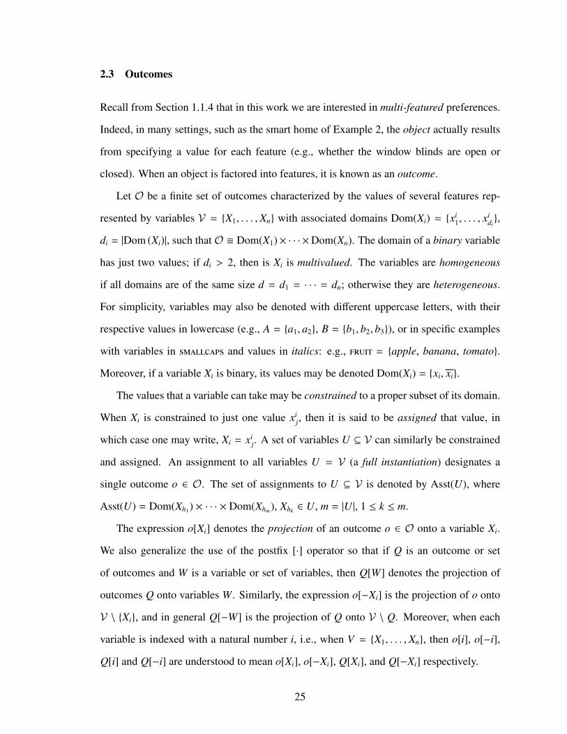
2.3 Outcomes
Recall from Section 1.1.4 that in this work we are interested in multi-featured preferences.
Indeed, in many settings, such as the smart home of Example 2, the object actually results
from specifying a value for each feature (e.g., whether the window blinds are open or
closed). When an object is factored into features, it is known as an outcome.
Let O be a finite set of outcomes characterized by the values of several features rep-
resented by variables V = X1, . . . , Xn with associated domains Dom(Xi) = xi1, . . . , x
idi,
di = |Dom (Xi)|, such that O ≡ Dom(X1)× · · · ×Dom(Xn). The domain of a binary variable
has just two values; if di > 2, then is Xi is multivalued. The variables are homogeneous
if all domains are of the same size d = d1 = · · · = dn; otherwise they are heterogeneous.
For simplicity, variables may also be denoted with different uppercase letters, with their
respective values in lowercase (e.g., A = a1, a2, B = b1, b2, b3), or in specific examples
with variables in smallcaps and values in italics: e.g., fruit = apple, banana, tomato.
Moreover, if a variable Xi is binary, its values may be denoted Dom(Xi) = xi, xi.
The values that a variable can take may be constrained to a proper subset of its domain.
When Xi is constrained to just one value xij, then it is said to be assigned that value, in
which case one may write, Xi = xij. A set of variables U ⊆ V can similarly be constrained
and assigned. An assignment to all variables U = V (a full instantiation) designates a
single outcome o ∈ O. The set of assignments to U ⊆ V is denoted by Asst(U), where
Asst(U) = Dom(Xh1) × · · · × Dom(Xhm), Xhk ∈ U, m = |U |, 1 ≤ k ≤ m.
The expression o[Xi] denotes the projection of an outcome o ∈ O onto a variable Xi.
We also generalize the use of the postfix [·] operator so that if Q is an outcome or set
of outcomes and W is a variable or set of variables, then Q[W] denotes the projection of
outcomes Q onto variables W. Similarly, the expression o[−Xi] is the projection of o onto
V \ Xi, and in general Q[−W] is the projection of Q onto V \ Q. Moreover, when each
variable is indexed with a natural number i, i.e., when V = X1, . . . , Xn, then o[i], o[−i],
Q[i] and Q[−i] are understood to mean o[Xi], o[−Xi], Q[Xi], and Q[−Xi] respectively.
25

The expression uxik denotes the combination of u ∈ Asst(U) and xi
k ∈ Dom(Xi), where
Xi < U. In general, if w and u are assignments to disjoint sets W and U, w ∈ Asst(W),
u ∈ Asst(U), W ∩ U = ∅, then wu denotes the combination of w and u.
Example 6. Let V = A, B,C, Dom(A) = a1, a2, a3, Dom(B) = b1, b2, and Dom(C) =
c1, c2. Then Asst(B,C) = b1c1, b1c2, b2c1, b2c2, a3b1c1[A] = a3, a3b1c1[B,C] = b1c1,
and a3b1c1[−C] = a3b1.
Definition 7 (Hamming distance). The Hamming distance of a pair of outcomes HD(o, o′),
o ∈ O, o′ ∈ O, is the number of variables in the outcomes for which the values differ, i.e.,
HD(o, o′) = | Xi : o[Xi] , o′[Xi] | . (2.1)
For example, HD(a3b1c1, a1b1c1) = 1 and HD(a1b1c1, a2b2c2) = 3. One can observe that
HD(o, o′) = HD(o′, o) for all o, o′ ∈ O and that HD(o, o′) = 0 if and only if o = o′. Finally,
0 ≤ HD(o, o′) ≤ n, where n = |V |.
We denote by On the set of all outcomes on n binary features and by On,d all outcomes
on n d-ary features. We denote by O2n and O2
n,d all ordered pairs of outcomes on n binary
and d-ary features. O2n | h and O2
n,d | h are the same sets restricted to pairs with Hamming
distance h, 0 ≤ h ≤ n; for example, O4 | 2 = (o, o′) : HD(o, o′) = 2, o ∈ O4, o′ ∈ O4.
2.4 Preferences and CP-nets
A preference relation takes the form of a preorder if it can model outcomes over which
a subject may be indifferent. In this work, however, strict (though not necessarily total)
preferences are assumed. We thus model preferences as a partial order.
Definition 8 (Preference). A strict preference relation S is a partial order on a set of
outcomes O by a subject S.
When no confusion would result, the subscript will be omitted and used as an infix
operator, where o o′ indicates that the subject strictly prefers o to o′. Equivalently one
26

may write o′ ≺ o, because o o′ ⇐⇒ o′ ≺ o. In a preference relation, as for partial
orders in general, the infix ‖ operator denotes incomparability. Recall from Section 2.1
that since preferences are posets, just one of the following is true: o o′, o ≺ o′, o = o′,
or o ‖ o′. We assume O is finite and can be factored as described in Section 2.3. Note
that for d-ary variables |O| = dn; that is, exponential space is required to store (see
1.2.1). However, because O is factored, a conditional preference network (CP-net) [16]
can compactly model .
Definition 9 (CP-net). A conditional preference network is a digraph on V = X1, . . . , Xn
in which each node is labeled with a conditional preference table. An edge (Xh, Xi) indicates
that the preferred value of Xi in depends on the value of its parent variable Xh.
Definition 10 (CPT). A conditional preference table CPT(Xi) consists of conditional ce-
teris paribus preference rules (CPRs) u : i specifying a linear order on Dom(Xi) for
assignments to the parents of Xi in the dependency graph, u ∈ Asst(Pa(Xi)).
Formally, CPT(Xi) implements a function f : Asst(Pa(Xi)) → S(Dom(Xi)). If f (u) is
defined for all u ∈ Asst(Pa(Xi)), i.e., a preference over Xi is specified for every assignment,
the CPT is said to be complete; otherwise it is incomplete. Unless otherwise specified, we
assume CPTs are complete. The expression CPT(Xi|Xh = xhk) denotes all rules of CPT(Xi)
of the form uxhk : i where xh
k ∈ Dom(Xh), Xh ∈ Pa(Xi), u ∈ Asst(Pa(Xi) \ Xh). Figure 2.3
illustrates a simple chain-shaped, binary-valued CP-net.
Weather Activity Friend
fair rain fair : cycling table tennisrain : table tennis cycling
cycling : emily henrytable tennis : henry emily
Figure 2.3: A Simple CP-net N
27

The size of a CPT is defined as the number of rules it contains, and the size of the
CP-net is the sum of the sizes of its CPTs. If domains are d-ary and CPTs are complete,
a node with m parents has dm CPRs. Thus, the size of the description is exponential in
the maximum indegree of G. To provide a compact model of (see 1.2.2), indegree is
assumed to be bounded by a small constant [16], i.e., |Pa (Xi)| ≤ c for all Xi. We assume
that domain size is similarly bounded.
The term dependency graph (or graph) denotes the digraph G of a CP-net apart from
its CPTs (tables). A chain, tree-shaped, or polytree CP-net is one for which the graph
takes the respective shape of a chain, directed forest, or polytree (Section 2.2). It is often
assumed that the graph of a CP-net is acyclic (i.e., a DAG); if the CP-net may have a cycle,
this is usually qualified, e.g., generally cyclic CP-nets.
As discussed in Section 1.2.1, a CP-net induces an exponentially larger graph known
as the preference graph (or outcome graph), which we now define formally:
Definition 11 (Preference graph). The induced preference graph (PG) of a CP-net N is a
digraph H = (O, C) in which (o′, o) ∈ C if and only if there exists a CPR u : i in the
CPT of a node Xi in N, such that (o[Xi], o′[Xi]) ∈ i, o[Xi] , o′[Xi], o[−Xi] = o′[−Xi],
u ∈ Asst(Pa(Xi)), u = o[Pa(Xi)] = o′[Pa(Xi)], o ∈ O, o′ ∈ O, and Xi ∈ V . A directed edge
from o′ to o thus indicates that HD(o, o′) = 1 and that o′ ≺ o.
If variables are binary, |O| = 2n and H takes the geometric shape of a directed hyper-
cube, sometimes known as a Hamming cube [31]. Figure 2.4 depicts the induced preference
graph for the CP-net of Figure 2.3. (Note that FCH, for example, denotes the outcome 〈fair,
cycling, henry〉.) The rule fair rain in the CPT of Weather in N induces the edges along
“dimension” Weather in H: (RCH, FCH), (RTH, FTH), (RCE, FCE), and (RTE, FTE).
This must be the case, since the subject always prefers fair weather to rain, regardless of
the activity or companion. Similarly, the rule table tennis : henry emily in CPT(friend)
induces the directed edges, (FTE, FTH) and (RTE, RTH). Whatever the Weather, the sub-
ject prefers henry to emily as the Friend for Activity table tennis.
28

FCE
FCH
FTE
FTH
RCE
RCH
RTE
RTH
Figure 2.4: Induced Preference Graph H of CP-net N (see Figure 2.3)
The CPRs allow direct comparison between outcomes that differ in the value of just
one variable. Comparing outcomes that differ in more than one variable requires finding
a path in the preference graph from the less to the more preferred outcome. For example,
the outcomes RCE and FCH differ in two variables; thus no single rule specifies whether
the subject would prefer a rainy day cycling with Emily or a fair day cycling with Henry.
However, note that a path connects the two outcomes:
RCE ≺ RTE ≺ RTH ≺ FTH ≺ FCH. (2.2)
Such a path is a known as an improving flipping sequence (FS), since traversing an edge
of the preference graph flips the value of a variable such that the subject is more satisfied
with the resulting outcome.3 Paths such as RCE FCH result from the transitive closure
of the ceteris paribus rules of the CP-net. The existence of such a path counts as a proof
that FCH RCE. Note that multiple paths may connect a pair of outcomes. For example,
FCE RCE since RCE ≺ RTE ≺ FTE ≺ FCE; however, there is also a shorter, more direct
path, RCE ≺ FCE.3While the term flip is perhaps better suited to binary domains (e.g., flip a coin), it is also used of
multivalued variables both in everyday speech (e.g., flip a die) and in the preference handling literature. Notethat the semantics of the rule u :i allow us to flip directly to any more preferred value in Dom(Xi) givenu. In particular, if CPT(B) contains the rule a1 : b1 b2 b3, one can flip directly from o′[AB] = a1b3 too[AB] = a1b1 without first having to visit o′′[AB] = a1b2.
29

Definition 12 (Flipping sequence). A flipping sequence is a path in the induced preference
graph of a CP-net.
In general, if there exists an improving flipping sequence from o′ to o, then we write
N |= o o′ and say the CP-net entails the dominance of o over o′ in the induced order. If
no path exists in either direction, i.e., if N |= o 6 o′ and N |= o′ 6 o, then we can reason
that the two outcomes are incomparable with respect to the CP-net; i.e., N |= o ‖ o′. The
search for such a path is known as dominance testing (DT).
Definition 13 (DT problem). A dominance testing problem is a decision problem for which
the input is a triple (N, o, o′) consisting of a CP-net N on V = X1, . . . , Xn and outcomes o
and o′, o ∈ O, o′ ∈ O, O ≡ Dom(X1) × · · · × Dom(Xn). The answer is in the affirmative if
and only if N |= o o′.
We denote by DT(N ,O) the set of all DT problem instances (N, o, o′), such that N ∈ N ,
o ∈ O, and o′ ∈ O, and by DT(N ,O | θ) the set of instances satisfying one or more
conditions θ. For example, DT(N ,O HD(o, o) = h, APL(G) = 0.5) denotes the set of DT
problem instances (N, o, o′), such that N ∈ N , o ∈ O, o′ ∈ O, for which the Hamming
distance between the outcomes is h and the average path length of the dependency graph is
0.5.
Definition 14 (Flipping length). The flipping length is the length of the shortest path be-
tween a pair of outcomes in the induced preference graph H of a CP-net N,
FL(N, o′, o) = minpathH(o′, o). (2.3)
If no such path (flipping sequence) exists, then the flipping length is undefined.
When the flipping sequence is undefined, we may write FL(N, o′, o) = ∞.
30

In Chapter 5 we will be interested in the longest flipping length, which we call the
diameter of the preference graph Diam(H) (see Definition 3).4 In the example shown in
Figure 2.4, the longest flipping sequence is the one given in Equation 2.2; consequently,
Diam(H) = 4. Note that the outcomes (RCE, FCH) that produce this diameter have Ham-
ming distance 2. We will also be interested in the longest flipping length that connects any
pair of outcomes with a given Hamming distance h.
Definition 15 (h-Diameter). The h-diameter of the induced preference graph H is
Diamh(H) = maxo,o′
∣∣∣minpathH(o, o′)∣∣∣ , (2.4)
such that HD(o, o′) = h, o ∈ O, o′ ∈ O.
One can confirm from Figure 2.4 that while Diam(H) = Diam2(H) = 4, the shortest path
between any two outcomes that differ in all three variables is Diam3(H) = 3.
Definition 16 (Mean flipping length). If I ⊆ DT(N ,O) is a non-empty set of DT problem
instances, then MFL(I) is the mean flipping length for I,
MFL(I) =1|I |
∑I∈I
FL(N, o, o′) (2.5)
such that o , o′ and FL(o, o′) is defined, where N, o and o′ are the three elements of tuple
I = (N, o, o′).
Similarly, MFL(I | θ) denotes the mean flipping length for instances I that satisfy a set of
conditions θ. For example, MFL(I | HD(o, o′) = 2) denotes the mean flipping length for
all I ∈ I with Hamming distance 2.
We denote by Nn the set of all CP-nets on n binary features, and by Nn,d the set of CP-
nets on n d-ary features. Nn | c and Nn,d | c indicate the same sets restricted to dependency
graphs with indegree at most c.4Confusingly, this longest flipping length is sometimes called the diameter of the CP-net [61]. However,
that usage lends itself to confusion between the diameter of the induced preference graph and the diameterof the dependency graph, Diam(G), which in this case of course is 2.
31

Belt
Shoes
black : black tantan : tan black
black : black tantan : tan black
(a) Consistent CP-net N
(black, black)
(black, tan) (tan, tan)
(tan, black)
(b) Consistent PG H
Belt
Shoes
black : black tantan : tan black
black : tan blacktan : black tan
(c) Inconsistent CP-net N′(black, black)
(black, tan) (tan, tan)
(tan, black)
(d) Inconsistent PG H′
Figure 2.5: Cyclic CP-nets and Induced Preference Graphs
Finally, one can observe that if H (not to be confused with G) contains a cycle, the in-
duced order on the outcomes is inconsistent. Consider the CP-nets in Figure 2.5. CP-net N
in Figure 2.5a expresses a preference for coordinating the color of leathers. (The customary
rule of fashion is that a black belt should be matched with black shoes, tan with tan, and so
on.) The induced preference graph expresses this convention as one would expect. If the
subject discovers that he is wearing a black belt and tan shoes, he can improve by switching
either shoes or belts. Having made the switch, the outcome is then one of the two incompa-
rable optima. A CP-net could just as easily enforce anti-coordination by inverting the order
in all four conditional preference rules. However, in CP-net N′ in Figure 2.5c, observe that
only the CPT for shoes is inverted. The unfortunate result, depicted in Figure 2.5d, is an
32

Table 2.1: Commonly Used Acronyms
Acronym Meaning Section
APL average path length 2.2
CP-net conditional preference network 2.4
CPR conditional preference rule 2.4
CPT conditional preference table 2.4
DAG directed acyclic graph (labeled) 2.2
DPSCG directed path singly connected graph 2.2
DT dominance testing 2.4
FS flipping sequence (improving) 2.4
HD Hamming distance 2.3
PG Preference graph 2.4
irrational subject who is forever changing shoes and belts in endless hope of improvement.
Unfortunately, if the graph G of a CP-net has cycles, finding optima and proving consis-
tency are known to be PSPACE-complete [42]. On the other hand, when G is acyclic, CPTs
are complete, and indifference is disallowed—assumptions that we will adopt throughout
most of this work—then the optimum outcome is unique, computationally easy to find, and
the resulting order on O is guaranteed to be consistent [16].
2.5 Commonly Used Notation and Abbreviations
The chapter concludes with references for the reader. Table 2.1 provides the meaning of
common acronyms. Table 2.2 summarizes notation commonly used throughout this work.
The Section column specifies the chapter, section, or subsection where the operator or term
is defined or discussed, if applicable.
33
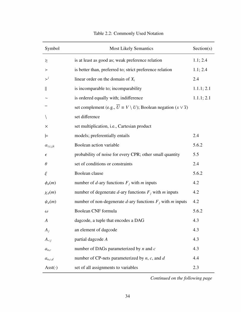
Table 2.2: Commonly Used Notation
Symbol Most Likely Semantics Section(s)
% is at least as good as; weak preference relation 1.1; 2.4
is better than, preferred to; strict preference relation 1.1; 2.4
i linear order on the domain of Xi 2.4
‖ is incomparable to; incomparability 1.1.1; 2.1
∼ is ordered equally with; indifference 1.1.1; 2.1
set complement (e.g., U ≡ V \ U); Boolean negation (x ∨ x)
\ set difference
× set multiplication, i.e., Cartesian product
|= models; preferentially entails 2.4
αt,i, j,k Boolean action variable 5.6.2
ε probability of noise for every CPR; other small quantity 5.5
θ set of conditions or constraints 2.4
ξ Boolean clause 5.6.2
φd(m) number of d-ary functions F j with m inputs 4.2
χd(m) number of degenerate d-ary functions F j with m inputs 4.2
ψd(m) number of non-degenerate d-ary functions F j with m inputs 4.2
ω Boolean CNF formula 5.6.2
A dagcode, a tuple that encodes a DAG 4.3
A j an element of dagcode 4.3
A< j partial dagcode A 4.3
an,c number of DAGs parameterized by n and c 4.3
an,c,d number of CP-nets parameterized by n, c, and d 4.4
Asst(·) set of all assignments to variables 2.3
Continued on the following page
34
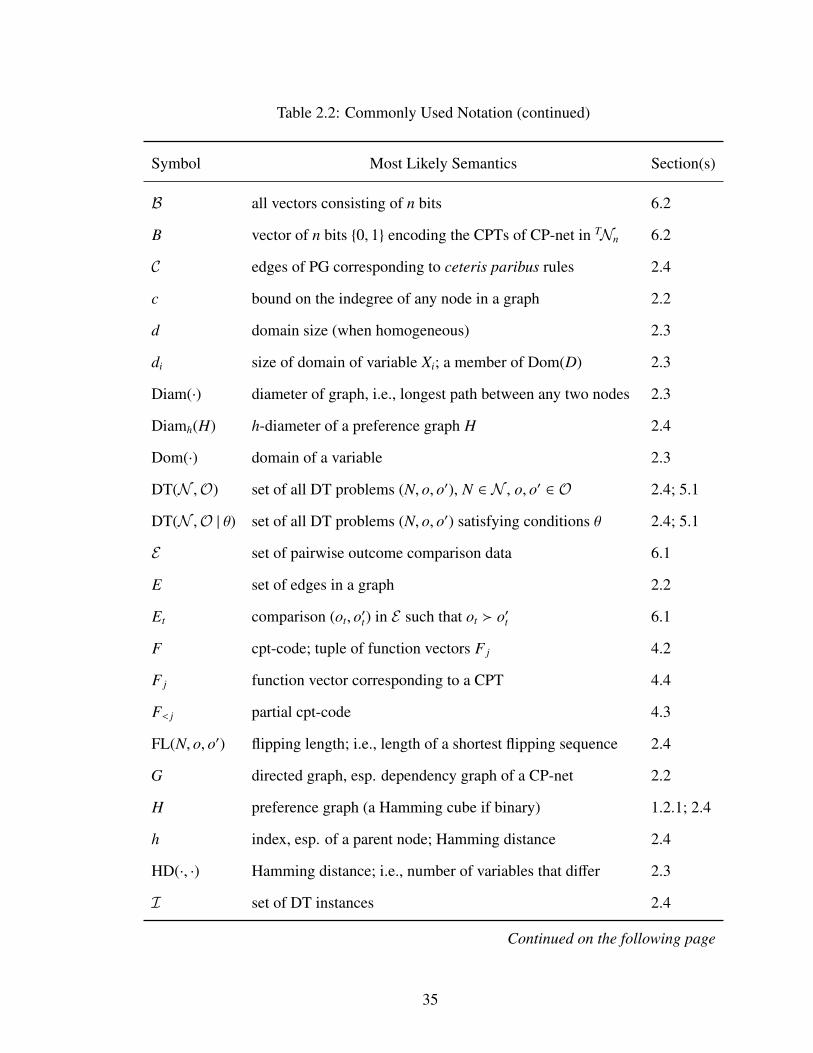
Table 2.2: Commonly Used Notation (continued)
Symbol Most Likely Semantics Section(s)
B all vectors consisting of n bits 6.2
B vector of n bits 0, 1 encoding the CPTs of CP-net in TNn 6.2
C edges of PG corresponding to ceteris paribus rules 2.4
c bound on the indegree of any node in a graph 2.2
d domain size (when homogeneous) 2.3
di size of domain of variable Xi; a member of Dom(D) 2.3
Diam(·) diameter of graph, i.e., longest path between any two nodes 2.3
Diamh(H) h-diameter of a preference graph H 2.4
Dom(·) domain of a variable 2.3
DT(N ,O) set of all DT problems (N, o, o′), N ∈ N , o, o′ ∈ O 2.4; 5.1
DT(N ,O | θ) set of all DT problems (N, o, o′) satisfying conditions θ 2.4; 5.1
E set of pairwise outcome comparison data 6.1
E set of edges in a graph 2.2
Et comparison (ot, o′t) in E such that ot o′t 6.1
F cpt-code; tuple of function vectors F j 4.2
F j function vector corresponding to a CPT 4.4
F< j partial cpt-code 4.3
FL(N, o, o′) flipping length; i.e., length of a shortest flipping sequence 2.4
G directed graph, esp. dependency graph of a CP-net 2.2
H preference graph (a Hamming cube if binary) 1.2.1; 2.4
h index, esp. of a parent node; Hamming distance 2.4
HD(·, ·) Hamming distance; i.e., number of variables that differ 2.3
I set of DT instances 2.4
Continued on the following page
35

Table 2.2: Commonly Used Notation (continued)
Symbol Most Likely Semantics Section(s)
I DT instance (N, o, o′) 2.4
i index, esp. of a variable or node representing a feature 2.3
j index, e.g., of a child node, encoding, etc. 2.3; 4.3
k bound on flipping length for DLDT; index 5.5
L square matrix consisting of all flipping lengths 5.2
Ln all Prufer codes with n − 1 integers ranging from 1 to n + 1 6.2
L average path length; other length; Prufer code 5.2; 6.2
` index; length of a sequence, data set, or path 2.2; 6.1
M adjacency matrix of a graph 5.2
m number of parents of a node; number of inputs to a function 2.4
MFL(I) mean flipping length of a set of DT instances 2.4; 5.1
MFL(I | θ) mean flipping length of DT instances satisfying conditions θ 2.4; 5.1
N a set of CP-nets 2.4
N a particular CP-net 2.4
n number of features, variables, nodes 2.3
Nn binary acyclic CP-nets with n nodes 5.1
Nn,d d-ary acyclic CP-nets with n nodes 5.1
Nn | c binary acyclic CP-nets with n nodes and indegree bound c 5.1
Nn,d | c d-ary acyclic CP-nets with n nodes and indegree bound c 5.1
TNn tree-shaped CP-nets on n binary nodes 6.2
O set of conceivable outcomes 2.3
On set of outcomes over n binary features 2.3
On,d set of outcomes over n d-ary features 2.3
Continued on the following page
36

Table 2.2: Commonly Used Notation (continued)
Symbol Most Likely Semantics Section(s)
O2n all pairs of outcomes over n binary features 2.3
O2n | h all pairs of outcomes over n binary features with HD h 2.3
O2n,d | h all pairs of outcomes over n d-ary features with HD h 2.3
Pa(·) parents of a node 2.2
S(·) symmetric group; set of all rankings, permutations 2.2
S , T , U various sets
S the subject, preference holder 1.1; 2.4
Tn set of all treecodes Ln × Bn 6.2
t index of items in a sequence; timestep in SATplan 5.6.2; 6.1
u node in a graph; utility function; assignment to parents 1.1.1; 2.2
V set of features, variables, nodes 2.2; 2.3
v node in a graph 2.2
Xi a particular feature, variable, node 2.3
zt,i, j Boolean state variable 5.6.2
Copyright c© Thomas E. Allen, 2016.
37

Chapter 3 Related Work
This chapter provides an overview of the present state of the research involving CP-nets.
Because most of that research applies various restrictions to the formalism, Section 3.1
summarizes restrictions that can be applied to models, such as limiting the shape of the
network, the size of domains, etc. Section 3.2 discusses the problem of finding optimal
outcomes given a CP-net and also that of finding the k-best outcomes. Section 3.3 consid-
ers the problem of checking whether a CP-net is consistent. Section 3.4 discusses problems
related to reasoning with CP-nets, such as dominance testing, ordering queries, and heuris-
tic methods, as well as the complexity of the reasoning problems. Section 3.5 considers the
problem of learning CP-nets from outcome comparison data or elicited queries and what is
known about the complexity of the respective problems. Section 3.6 discusses experiments
with CP-nets, including efforts to generate CP-nets randomly, experimental validation of
algorithms, and available datasets. Section 3.7 concludes the chapter with a discussion of
some proposed extensions to the CP-net formalism.
3.1 General and Restricted CP-net Models
CP-nets have already been discussed along with examples in Sections 1.3 and 2.4. The
CP-net formalism was originally proposed by Craig Boutilier along with coauthors Ronen
I. Brafman, Carmel Domshlak, Holger H. Hoos, and David Poole, initially in conference
proceedings (1999) [17] and later extended for publication in the Journal of Artificial Intel-
ligence Research (2004) [16]. In their most general form, without extensions such as those
discussed in Section 3.7, CP-nets are allowed to have cycles in the dependency graph, with
only two constraints on the geometry: loops are disallowed, and a small constant bound on
indegree is assumed. Moreover, the features that characterize the outcome space, so long
as they are discrete, can be multivalued, CPTs can be partially specified (i.e., incomplete),
38

and CPRs can express a weak total order over the domain of the local variable. While such
general models can represent a broader range of problems, reasoning with such models
may be intractable and there is no guarantee that the resulting order on outcomes will be
consistent.
Almost always, however, one or more restrictions are applied to the set of possible
CP-net models, either as a requirement for algorithms or as an aid in proving theoretical
results. Restrictions can be applied to the dependency graph, domains, CPTs, or CPRs.
Recall from Sections 2.2 and 2.4 that the dependency graph of a CP-net can be restricted
to a subclass of digraphs, such as DAGs, polytrees, etc. Table 3.1 lists some of the more
common restrictions to the structure of the dependency graph. By far the most common
of these is to exclude cycles; in fact, unless qualified (e.g., generally cyclic CP-nets), one
can usually assume that the dependency graph is a DAG. Recall from Section 2.4 that,
regardless of the type of graph, a bound on indegree is always assumed for CP-nets to
ensure a compact model.
Similar restrictions can be applied to the variable domains, such as a bound on the
cardinality of the largest domain or on the number of different cardinalities when domains
are heterogeneous. A rather common restriction is that all variables must be binary [29, 61,
65, 104]. Another common restriction [16] is that CPTs must be complete, i.e., each CPT
is fully specified with a linear order over the local variable for every assignment to parents.
Algorithms for learning are an interesting exception in which it is common to output a
CP-net that is likely to be incomplete [29, 48, 58]. Finally, almost all researchers disallow
indifference, restricting attention to CP-nets that can model only strict preferences.
3.2 Finding Most Preferred Outcomes
A common problem in working with preferences is to find the (or in some cases, such as
Figure 2.5b, an) outcome that the subject most prefers. For other compact formalisms (see
Section 1.2.2), optimization problems of this type are known to be hard [32, 71]. However,
39

Table 3.1: CP-nets Characterized by Dependency Graph
Dependency Graph Resulting Class of CP-net ReferencesChain Chain CP-net [16]Antichain Separable CP-net (SCP-net) [66]Directed forest Tree (or Tree-structured) CP-net [11, 16, 59]Polytree Polytree CP-net [16]DPSCG Directed path singly connected CP-net [16]Max-δ-connected Max-δ-connected CP-net [16]DAG Acyclic CP-net [16]Digraph CP-net (or generally cyclic CP-net) [16, 42, 61]
Boutilier et al. [16] proved that the problem of outcome optimization is easy in acyclic,
complete CP-nets. In such cases the most preferred outcome is unique and can be found in
linear time in the number of nodes using a forward sweep algorithm that they describe.
Brafman et al. [20] proved that the related problem of finding the k-best outcomes in an
acyclic CP-net (presumably with complete CPTs) can be computed in polynomial time in
the number of variables, assuming the solutions can be linearized in a particular way, which
they call a contextual lexicographical linearization. If CPTs are incomplete, however, the
complexity of finding the most preferred and k-best outcomes is believed to be an open
problem [16].
3.3 Checking for Consistency
As noted in Section 2.4, CP-nets can induce an intransitive order on outcomes in certain
cases. In particular, as noted in Section 2.4, inconsistency can sometimes arise if the de-
pendency graph contains a cycle (see Figure 2.5). Domshlak and Brafman [30] showed
that consistency checking could be conducted efficiently for a wide class of cyclic, bi-
nary CP-nets. As later shown by Goldsmith et al. [42], however, the general problem is
PSPACE-complete. More recently, Santhanam et al. [93, 94] have reduced the problem to
one of model checking in the form of the CRISNER CP-nets reasoning tool.
40

3.4 Reasoning with CP-nets
Given a pair of distinct outcomes, the reasoning problem involves determining which
outcome, if either, is preferred. Section 3.4.1 discusses dominance testing, the strongest
method of reasoning. Section 3.4.2 then considers the weaker method or ordering queries.
Finally, heuristic methods are discussed in Section 3.4.3.
3.4.1 Dominance Testing
Recall from Section 2.4 that, given a CP-net N with strict preferences and a pair of out-
comes o and o′, dominance testing (DT) determines whether there exists an improving
flipping sequence from o′ to o. If so, the CP-net said to entail that the first outcome domi-
nates the second, written N |= o o′.
For arbitrary, possibly cyclic CP-nets, DT is known to be PSPACE-complete [42], and
in certain cases (in particular, chain CP-nets) flipping lengths can be Ω(2n/2), i.e., exponen-
tial in the number of nodes n, provided tables are incomplete and domains are multivalued,
even for chain CP-nets [16]. However, Boutilier et al. showed that, in the most general case,
dominance testing can be formulated as a STRIPS-type planning problem. More recently,
Kronegger et al. [61] have established several fixed parameter tractability (FPT) results for
dominance testing in a generalized class of CP-nets (GCP-nets) (similar to those studied
by [42]). Many of their FPT results also apply to CP-nets.
Several tractable subclasses for DT are known. Boutilier et al. [16] showed that DT can
be conducted in Θ(n2) time for binary valued tree CP-nets with their DT-Tree algorithm,
which also returns a flipping sequence if one exists. They claim that the algorithm remains
complete, with the same time complexity, when CPTs are incomplete. Bigot et al. [11]
subsequently described an algorithm they claim can answer dominance in O(n) time for
the same class of CP-nets (except that CPTs must also be complete), an unexpected result,
since the flipping length is O(n2) for such CP-nets. Thus, while the decision problem can
be answered in linear time, computing the flipping sequence itself requires quadratic time.
41

Table 3.2: Computational Difficulty of Dominance Testing
Graph Domains CPTs DT Complexity Running Time ReferencesDirected Forest Binary Complete P O(n) [11]Directed Forest Binary * P O(n2) [16]Directed Forest * * NP-hard ? [16]Polytree Binary * P O(22cn2c+3) [16]DPSCG Binary * NP-complete ? [16]Max-δ-connected Binary * NP-complete ? [16]* * * PSPACE-complete ? [42]*No restriction
In the case of polytree CP-nets, Boutilier et al. [16] showed that DT could be answered
in polynomial time via their reduction to planning. Specifically, the algorithm requires time
O(22cn2c+3) where c is the assumed bound on indegree in the dependency graph. How-
ever, even when variables are binary, DT for directed-path singly connected CP-nets is
NP-complete if CPTs are complete (and NP-hard otherwise). The problem remains NP-
complete when the number of paths between any two nodes in the graph is polynomially
bounded (i.e., max-δ-connected graphs). Table 3.2 summarizes the computational com-
plexity and running times of DT algorithms for various classes of CP-nets.
3.4.2 Ordering Queries
Because dominance testing is hard in many cases, Boutilier et al. [16] also introduced
a weaker, incomplete method of reasoning with CP-nets. Rather than asking whether a
flipping sequence exists between a pair of outcomes, the method searches for local rules
that would contradict the existence of such a sequence. Given a CP-net N and a pair of
outcomes o and o′, o is said to be consistently orderable over o′ if N 6|= o′ o. They call
this search for local contradictions an ordering query and show that it can be completed
in linear time in the number of variables, provided CPTs are complete. (The complexity
of ordering queries for incomplete CP-nets seems to be an open problem. However, the
authors note that they suspect it is hard.) Let N |=oq o o′ denote that o is consistently
orderable over o′ with respect to CP-net N. Note that N |=oq o o′ =⇒ N 6|= o′ o.
42

However, when N 6|=oq o o′ ∧ N 6|=oq o′ o, it could still be the case that N |= o o′,
N |= o′ o, or N |= o ‖ o′.
To better understand the nature of this method of ordering, recall that a CP-net induces
a partial order on outcomes. If o is consistently orderable over o′, it means only that o is
ordered before o′ in some linear extension of the induced partial order (see Section 1.1.2).
However, if o dominates o′, then it follows that o is ordered before o′ in every such linear
extension.
3.4.3 Reductions and Heuristic Methods
In general, DT involves a search for a flipping sequence that connects the two outcomes.
Any of the familiar search methods in AI, e.g., iteratively deepening depth-first search,
can be employed. Boutilier et al. [16] introduced two methods of pruning the search tree,
suffix fixing and forward pruning, that work in all cases, as well as a heuristic method,
least-variable flipping, that is incomplete except for binary-valued tree-shaped CP-nets. In
addition to the reduction to STRIPS-type planning [16], DT problems can also be reduced
to model checking [92, 93] (similar to their reduction for the consistency problem; see
Section 3.3). Finally, Li et al. [68] have proposed a heuristic approach to DT in acyclic,
generally multivalued CP-nets that they call DT*. While the algorithm is inspired by A*,
it does not seem to guarantee optimality; i.e., it does not always return a shortest flipping
sequence.
3.5 Learning CP-nets
Recall from Section 1.2.3 that, aside from direct construction by the subject, which is
problematic since it relies on introspection, learning a CP-net can take the form of active
elicitation or passive learning from data. The earliest work on learning CP-nets seems to be
that of Athienitou and Dimopoulos for the MPREF-2007 conference [6]. They introduced
a passive learning algorithm that attempts to recover a CP-net that entails all examples
43
in a set of outcome comparison data. However, as observed by Lang and Mengin [65],
entailment is an exceptionally strong requirement. Suppose a subject has a linear order
on the outcome space, arising from some utility function (see 1.1.1). Arguably, then, the
goal is not to “recover” some presumed original CP-net, but to learn a CP-net such that
the observed comparison data are consistent with the learned model. They proposed three
notions of consistency for CP-nets. Lang and Mengin were also among the first to study the
complexity of the learning problem. To establish a lower bound, they proposed a simple
class of so-called separable CP-nets (SCP-nets) for which the dependency graph is an
antichain, i.e., a graph with no edges. In a later paper [66] they succeeded in proving that,
while it was possible to answer in polynomial time whether there exists a binary-valued
SCP-net that entails all examples, the problem of deciding whether there exists such a
network that is weakly consistent with all examples is NP-complete.
Meanwhile, Koriche and Zanuttini explored a somewhat different learning problem,
that of active elicitation. They framed the problem as one of Angluin-style learning, at-
tempting to elicit CP-nets via adaptively generated swap queries, i.e., comparisons in which
the two outcomes differ in the value of just one variable (as in flipping sequences) [58, 59].
Among their contributions was introducing the concept of query complexity. Rather than
defining complexity in terms of computation size, they defined an attribute efficient algo-
rithm as one for which the number of queries is polynomial in the number of variables.
They also described Angluin-style membership and equivalence queries for CP-nets: the
relationship between the two types of queries is analogous to that of ordering queries and
dominance testing for reasoning with CP-nets. Koriche and Zanuttini showed that it was
not possible to learn a CP-net with equivalence queries alone, but that membership queries
were also required. They presented an algorithm showing it was possible to learn binary-
valued tree-structured CP-nets in an efficient manner given this definition.
Dimopoulos et al. continued work on the problem of learning CP-nets passively from
data, improving on their research from a few years before. They introduced an algorithm
44

that attempted to learn an acyclic, binary-valued CP-net that was consistent with all out-
come comparisons in a preexisting database [29]. Their algorithm first attempted to identify
variables over which the subject’s preferences were unconditional (those with 0 parents),
then variables with 1 parents, 2, and so on, until a node for each variable had been added
to the model.
A crucial step for each node involves determining whether a prospective set of nodes
could be the parents of the node under consideration. To determine this, the authors pro-
pose constructing a 2SAT instance, which is solvable in linear time, such that the solution
provides a CPT and establishes a position in the network for the node that is consistent with
all available comparison data. However, in some cases the algorithm may output failure in-
stead of a CP-net. Additionally, in the worst case the algorithm could iterate an exponential
number of times in the number of variables. They also proved that the problem of learn-
ing a CP-net consistent with comparison data was hard even for acyclic, binary CP-nets to
which other simplifying assumptions had been applied.
Recently Guerin et al. [47, 48] have proposed an elicitation algorithm for learning CP-
nets from user queries. The algorithm is similar in many respects to that of Dimopoulos
and Athienitou, but employs active elicitation rather than passive learning. The algorithm
is also distinctive in that it allows subjects to introspect on their preferences by asking for
a default, most-preferred value for each variable.
One of the problems inherent in learning preferences from human subjects is the pos-
sibility of noise or comparison data that are ultimately inconsistent through transitive clo-
sure. Liu et al. [70] propose maximizing the number of outcome comparisons that can be
included using a branch-and-bound approach. The method they propose—which is not
restricted to binary-valued domains—first learns a preference graph for the subject, then
constructs a CP-net from the preference graph. They claim that their algorithm runs in time
polynomial in the size of the preference graph. However, recall that the size of the pref-
erence graph is exponential in the number of features. Moreover, because the algorithm
45

employs a branch-and-bound method, it seems unlikely that it is polynomial even in the
size of the preference graph; it seems more likely that the worst-case running time is actu-
ally doubly exponential in the number of features. In their conclusion, Liu et al. mention
the possibility of exploiting an approximation method rather than branch-and-bound for
learning CP-nets from possibility inconsistent data. While this is an interesting proposal, I
am not yet aware of any algorithm that exploits such a method or of theoretical results on
the complexity of the problem of approximating CP-nets.
Finally, Cornelio et al. have explored the possibility of updating a learned CP-net after
additional data have been collected, without recreating it entirely [25, 26].
3.6 Experiments with CP-nets
Proposed CP-net algorithms are typically evaluated with theoretical proofs, experiments,
or both; Table 3.3 summarizes several studies involving CP-net learning or reasoning and
the methods of evaluation. Ideally, algorithms would be evaluated at least in part using ac-
tual CP-nets obtained from human subjects. Unfortunately, no such datasets are presently
available [3]. Datasets from which CP-nets can be learned are also problematic. The
PrefLib preference data repository [75], for example, provides only two combinatorial
preference datasets. One consists of approval ballots and ratings for candidates in the
2002 French election; the other consists of hotel reviews submitted to the Trip Advisor
travel site. However, it is unclear how these could be used to construct CP-nets for an
experiment, and to date neither dataset has been cited in any CP-net study. The SUSHI
preference dataset [53], consisting of user’s ratings, ranking, and the feature composition
of different types of sushi, has been adapted by at least one team of authors for their CP-net
learning algorithms [69, 70]. However, this sort of adaptation, while fairly common in the
computational social choice and preference learning communities, involves numerous data
modeling decisions that can undermine the validity of such experiments [81, 84]. While
Allen et al. [3] describe a rigorous psychological experiment on whether human prefer-
46

Table 3.3: Evaluation Methods for Proposed CP-net Algorithms
Study Rea
soni
ng
Lea
rnin
g
Proo
fs
Synt
hetic
Dat
a
Rep
urpo
sed
Dat
a
Allen [1] X X X XBigot et al. [11] X XBigot et al. [12] X XBoutilier et al. [16] X XDimopoulos et al. [29] X XEckhardt and Vojtas [33, 34] X XGuerin et al. [47] X XKoriche and Zanuttini [58, 59] X XKronegger et al. [61] X X XLi et al. [68] X X XLiu et al. [69, 70] X X X XSanthanam et al. [92] X X X
ences can be consistently modeled with CP-nets, the results of that experiment are not yet
available. Therefore, due to the lack of suitable real-world data, researchers often rely on
synthetic datasets. However, as discussed in detail in Chapter 4, synthetic data are also
problematic due to naıve generation methods.
3.7 Extensions to the Formalism
We conclude with a brief discussion of a few of the many proposed extensions to the CP-net
formalism—GCP-nets, TCP-nets, mCP-nets, and PCP-nets.
• General CP-nets (GCP-nets) dispense with the explicit graphical structure of clas-
sical CP-nets and consist only of a set of conditional preference rules. Such a for-
malism is helpful for networks that may contain cycles and be highly complex in the
interrelationships among nodes. As such, GCP-nets can facilitate the proof of certain
complexity results and were employed both in the PSPACE-completeness proofs of
Goldsmith et al. [42, 43] and in the FPT results of Kronegger et al. [61].
47

• Tradeoffs-enhanced CP-nets (TCP-nets), introduced by Brafman et al. [19], ex-
tends the CP-net formalism by allowing the model to reflect the relative importance
assigned to the features. In addition to the directed edges indicating conditional de-
pendencies, the model includes two additional types of edges: importance arcs, di-
rected edges showing that one variable is more important to the subject’s satisfaction
than the other, and conditional importance arcs, indicating the relative importance of
variables given the values assigned to other nodes in the graph. While the proposed
formalism is highly expressive, its greater complexity (at least for human users) has
perhaps limited its adoption.
• mCP-nets were conceived by Rossi et al. [89] as a formalism for representing the
preferences of multiple agents. The preferences of m individual agents are repre-
sented as a partial CP-net, and the semantics of the aggregated mCP-net are related
to voting. Recently, Lukasiewicz and Malizia [72] have studied the computational
complexity of various problems involving mCP-nets.
• Probabilistic CP-nets (PCP-nets) were proposed by Cornelio [26] and later refined
by Bigot et al. [11] and Cornelio et al. [25]. Whereas CP-nets are deterministic,
PCP-nets assign a probability to every conditional preference rule. PCP-nets are
presently limited to O-legal structures with strict preferences over binary domains
and complete CPTs. Such networks assume that the probabilities of each node are
independent and hence that the probabilities of edges can be calculated using the
product rule. Cornelio [26] has also explored the connection between PCP-nets and
Bayesian networks. Based on this close relationship with Bayesian networks, Bigot
et al. [12] have subsequently shown that PCP-nets can be learned in polynomial time
from a set of optimal outcomes when the dependency graph is tree-shaped.
Copyright c© Thomas E. Allen, 2016.
48
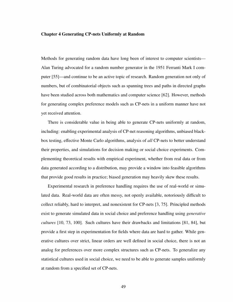
Chapter 4 Generating CP-nets Uniformly at Random
Methods for generating random data have long been of interest to computer scientists—
Alan Turing advocated for a random number generator in the 1951 Ferranti Mark I com-
puter [55]—and continue to be an active topic of research. Random generation not only of
numbers, but of combinatorial objects such as spanning trees and paths in directed graphs
have been studied across both mathematics and computer science [62]. However, methods
for generating complex preference models such as CP-nets in a uniform manner have not
yet received attention.
There is considerable value in being able to generate CP-nets uniformly at random,
including: enabling experimental analysis of CP-net reasoning algorithms, unbiased black-
box testing, effective Monte Carlo algorithms, analysis of all CP-nets to better understand
their properties, and simulations for decision making or social choice experiments. Com-
plementing theoretical results with empirical experiment, whether from real data or from
data generated according to a distribution, may provide a window into feasible algorithms
that provide good results in practice; biased generation may heavily skew these results.
Experimental research in preference handling requires the use of real-world or simu-
lated data. Real-world data are often messy, not openly available, notoriously difficult to
collect reliably, hard to interpret, and nonexistent for CP-nets [3, 75]. Principled methods
exist to generate simulated data in social choice and preference handling using generative
cultures [10, 73, 100]. Such cultures have their drawbacks and limitations [81, 84], but
provide a first step in experimentation for fields where data are hard to gather. While gen-
erative cultures over strict, linear orders are well defined in social choice, there is not an
analog for preferences over more complex structures such as CP-nets. To generalize any
statistical cultures used in social choice, we need to be able to generate samples uniformly
at random from a specified set of CP-nets.
49

This chapter introduces a method for generating acyclic CP-nets uniformly at random.
A key idea of this method is that the structure of a CP-net is equivalent to a tuple of sets
representing the parents of nodes in the network. We will consider how to enumerate all
such dagcodes, as these tuples are known [99],1 and how to calculate the number of CP-
nets—the possible graphs and conditional preference tables (CPTs)—that extend a partial
dagcode. The resulting novel recurrence makes it possible to generate the graph and CPTs,
node by node, such that all CP-nets with a given domain size and bound on indegree are
equiprobable.
Section 4.1 highlights two problems, bias and degeneracy, that result from commonly
used naıve generation methods. Section 4.2 shows how to encode and avoid degeneracy in
the CPTs. Section 4.3 explains how to encode and count the dependency graphs. These
results are then brought together in Section 4.4 to create an algorithm that samples the
space of CP-nets uniformly. Section 4.5 shows how to sample uniformly from outcomes
and the set of dominance testing problem instances. Note that in this chapter it is assumed
that domains are homogeneous but possibly multivalued, i.e., d = d1 = · · · = dn, where
di = |Dom (Xi)|, for all Xi ∈ V , and that the CPTs are complete, i.e., have dm rules, one
for every assignment to the m parents, m = |Pa (Xi)|. Notation is discussed in detail in
Chapter 2; in particular, see Table 2.2.
4.1 Naıve Generation, Bias, and Degeneracy
If one wants to generate CP-nets without regard for the resulting distribution, many simple
random methods exist. For example, initialize a CP-net with n nodes, no edges, and empty
CPTs; choose a random subset of pairs (Xh, Xi), h < i, inserting an edge from each Xh to Xi;
generate a CPT for each Xi with d|Pa(Xi)| rules, each a random permutation of the d values
of Xi; and randomly permute the n labels. One suspects that something along these lines is
meant when a paper states, “We generated 1000 CP-nets at random.” However, this naıve1I use dagcode rather than DAG code (as in [99]) so as to better emphasize whether I am referring to the
encoding or to the DAG itself.
50
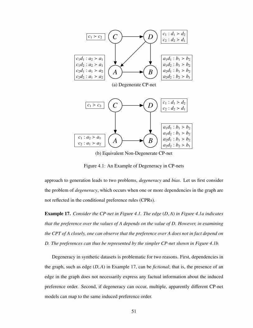
A B
C D
c1d1 : a2 a1
c1d2 : a2 a1
c2d1 : a1 a2
c2d2 : a1 a2
a1d1 : b1 b2
a1d2 : b1 b2
a2d1 : b1 b2
a2d2 : b2 b1
c1 c2c1 : d1 d2
c2 : d2 d1
(a) Degenerate CP-net
A B
C D
c1 : a2 a1
c2 : a1 a2
a1d1 : b1 b2
a1d2 : b1 b2
a2d1 : b1 b2
a2d2 : b2 b1
c1 c2c1 : d1 d2
c2 : d2 d1
(b) Equivalent Non-Degenerate CP-net
Figure 4.1: An Example of Degeneracy in CP-nets
approach to generation leads to two problems, degeneracy and bias. Let us first consider
the problem of degeneracy, which occurs when one or more dependencies in the graph are
not reflected in the conditional preference rules (CPRs).
Example 17. Consider the CP-net in Figure 4.1. The edge (D, A) in Figure 4.1a indicates
that the preference over the values of A depends on the value of D. However, in examining
the CPT of A closely, one can observe that the preference over A does not in fact depend on
D. The preferences can thus be represented by the simpler CP-net shown in Figure 4.1b.
Degeneracy in synthetic datasets is problematic for two reasons. First, dependencies in
the graph, such as edge (D, A) in Example 17, can be fictional; that is, the presence of an
edge in the graph does not necessarily express any factual information about the induced
preference order. Second, if degeneracy can occur, multiple, apparently different CP-net
models can map to the same induced preference order.
51

B
A
b b
b : a ab : a a
(a) One Edge
ab
ab ab
ab
(b) Induced PG
A
B b b
a a
(c) No Edge
Figure 4.2: Degeneracy Can Violate Basic Assumptions of an Experiment
Example 18. Suppose a researcher wants to test a new DT algorithm to understand how
running time varies as the number of edges in the network increases. (Also, he thinks a nice
bar chart will impress reviewers.) As a first step, he generates two sets of CP-nets using a
naıve approach. The CP-nets in each set have binary domains and two nodes; the first set
has just one edge, and the second set has no edge. However, if each CPR is assigned in the
manner of a coin flip, an expected 50% of the CP-nets in the first set will be degenerate like
the one in Figure 4.2a. As such, its induced preference graph, shown in Figure 4.2b, will be
identical to that of the no-edge CP-net in Figure 4.2c. Thus, one of the basic assumptions
of the experiment, that the two sets induce different preference orders, is violated.
Naıve generation methods also result in another problem that can violate the basic as-
sumptions of experiments: statistical bias. To understand this bias, consider the following
dependency graphs and their associated CP-net counts2 as shown in Figure 4.3. Both graphs
have 5 nodes and 5 edges, but the number of CP-nets associated with each graph differs
greatly. Observe that for the chain-shaped graph on the left, when d = 2, there are just two
ways to choose each of the n CPTs such that they are consistent with the dependency graph.
The CPT of root E could be [e1 e2] or [e2 e1]. The other nodes, each of which has
only one parent, also have two (non-degenerate) possibilities for their CPT; e.g., CPT(A)
could be [b1 : a1 a2, b2 : a2 a1] or [b1 : a2 a1, b2 : a1 a2]. However, in the2The CP-net counts for G and G′ are ψd(0)(ψd(1))4 and (ψd(0))4ψd(4), respectively, where ψd(m) is the
number of non-degenerate CPTs with m parents and d-ary domains, as discussed in Section 4.2.
52

E B A D C
Chain-shaped graph G
D′ A′ B′
E′
C′
Star-shaped graph G′
(a) Dependency Graphs that Differ in Maximum Indegree
d CP-nets with G CP-nets with G′
2 32 1.03× 10⁶
3 7,776 1.39× 1066
4 7,962,624 7.16× 10358
5 24,883,200,000 6.38× 101307
(b) Number d-ary CP-nets for Dependency Graphs above
Figure 4.3: How Naıve Generation Can Lead to Bias
case of the star-shaped graph on the right, CPT(A′) has d4 = 16 rules, each with d! = 2
possible orderings. In all, over one million CP-nets have the graph on the right, while only
32 have the graph on the left. Further observe that the ratio of this imbalance very rapidly
increases with the domain size d. Thus, if the algorithm above in fact generated the two
graphs with equal likelihood, it would grossly oversample CP-nets with the first graph,
while correspondingly undersampling those with the second.
However, the naıve algorithm does not even generate the two DAGs with equal likeli-
hood. Because there are 5! = 120 ways to permute the labels of the first DAG, but only 5
ways to permute those of the second, the star-shaped DAG on the right would be generated
24 times as often as the chain-shaped DAG on the left. Despite this, the CP-nets in the
star-shaped case would still be greatly undersampled.
53

CPT(A)c1d1 : a2 a1
c1d2 : a2 a1
c2d1 : a1 a2
c2d2 : a1 a2
In1 In2 F0 0 10 1 11 0 01 1 0
Figure 4.4: CPT and Corresponding Boolean Function
4.2 Counting and Generating the CPTs
The notion of a degenerate CPT introduced in Section 4.1 can be generalized with the help
of a bijection (a mapping that is one-to-one and onto) with discrete multivalued functions.
One can model each CPT(Xi) as a function f : 0, . . . , d − 1m → 0, . . . , d! − 1, where
m = |Pa (Xi)|. The inputs correspond to the values of the m parents of Xi. The output
corresponds to one of the d! orders of the domain of Xi.
Observe that if variables are binary (d = 2), f is a Boolean function. In that case the
values xh1 and xh
2 of each parent Xh can map to 0 and 1 respectively. The two possible linear
orders xi1 xi
2 and xi2 xi
1 can correspond to outputs 0 and 1. One can thus model the
degenerate CPT of node A from Example 17 with the truth table in Figure 4.4.
If variables are multivalued, the mapping is similar, as illustrated in Figure 4.5 for a
CPT with two parents and three-valued domains. Note that the inputs to the multivalued
function are in the range (0 . . d − 1), while the outputs are in the range (0 . . d! − 1). For
mapping the outputs, one can use Lehmer codes [67] (see also the discussion of the factorial
number system by Knuth [56, 3.2.2 Alg. P]), as illustrated in the table on the right-hand
side of Figure 4.5 for d = 3.
Thus, any CPT can be encoded as an equivalent function vector F of length dm. Note
that the values in the input columns of Figures 4.4 and 4.5 are only for the benefit of the
human reader and need not be represented explicitly. The entries in a function vector are or-
dered according to a radix d positional numbering system, where each digit corresponds to
the value of a parent variable. Of course, to produce the corresponding CPT from a vector,
one would also need to know the labels of the variable, parent variables, and domains.
54
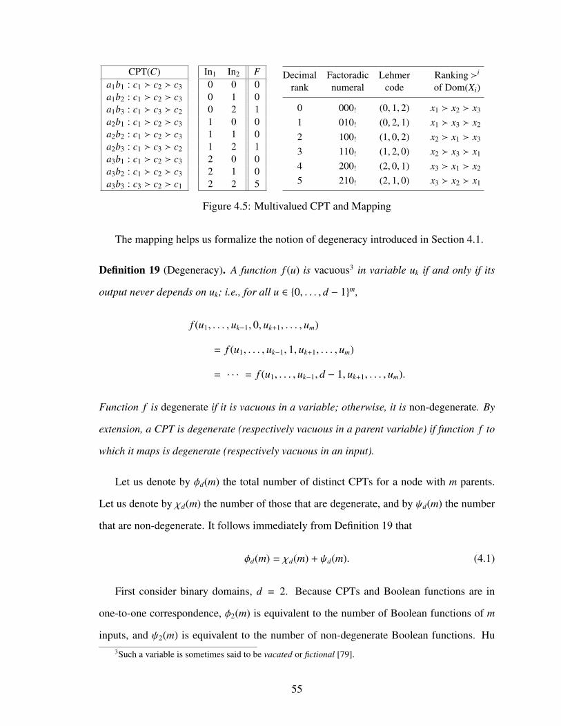
CPT(C)a1b1 : c1 c2 c3a1b2 : c1 c2 c3a1b3 : c1 c3 c2a2b1 : c1 c2 c3a2b2 : c1 c2 c3a2b3 : c1 c3 c2a3b1 : c1 c2 c3a3b2 : c1 c2 c3a3b3 : c3 c2 c1
In1 In2 F0 0 00 1 00 2 11 0 01 1 01 2 12 0 02 1 02 2 5
Decimal Factoradic Lehmer Ranking i
rank numeral code of Dom(Xi)
0 000! (0, 1, 2) x1 x2 x3
1 010! (0, 2, 1) x1 x3 x2
2 100! (1, 0, 2) x2 x1 x3
3 110! (1, 2, 0) x2 x3 x1
4 200! (2, 0, 1) x3 x1 x2
5 210! (2, 1, 0) x3 x2 x1
Figure 4.5: Multivalued CPT and Mapping
The mapping helps us formalize the notion of degeneracy introduced in Section 4.1.
Definition 19 (Degeneracy). A function f (u) is vacuous3 in variable uk if and only if its
output never depends on uk; i.e., for all u ∈ 0, . . . , d − 1m,
f (u1, . . . , uk−1, 0, uk+1, . . . , um)
= f (u1, . . . , uk−1, 1, uk+1, . . . , um)
= · · · = f (u1, . . . , uk−1, d − 1, uk+1, . . . , um).
Function f is degenerate if it is vacuous in a variable; otherwise, it is non-degenerate. By
extension, a CPT is degenerate (respectively vacuous in a parent variable) if function f to
which it maps is degenerate (respectively vacuous in an input).
Let us denote by φd(m) the total number of distinct CPTs for a node with m parents.
Let us denote by χd(m) the number of those that are degenerate, and by ψd(m) the number
that are non-degenerate. It follows immediately from Definition 19 that
φd(m) = χd(m) + ψd(m). (4.1)
First consider binary domains, d = 2. Because CPTs and Boolean functions are in
one-to-one correspondence, φ2(m) is equivalent to the number of Boolean functions of m
inputs, and ψ2(m) is equivalent to the number of non-degenerate Boolean functions. Hu3Such a variable is sometimes said to be vacated or fictional [79].
55

Table 4.1: Values of φ2(m) and ψ2(m) for m = 0 to 5
m φ2(m) χ2(m) ψ2(m)χ2(m)φ2(m)
ψ2(m)φ2(m)
0 2 0 2 0.0000 1.0000
1 4 2 2 0.5000 0.5000
2 16 6 10 0.3750 0.62503 256 38 218 0.1484 0.85164 65,536 942 64,594 0.0144 0.98565 4,294,967,296 325,262 4,294,642,034 0.0001 0.9999
[51, §2] (see also the work of Harrison [50] and O’Connor [79]) proved that for Boolean
functions
φ2(m) = 22m, (4.2)
and
ψ2(m) =
m∑k=0
(−1)m−k
(mk
)22k. (4.3)
Table 4.1 shows the values of φ2(m) [98, A001146] ψ2(m) [98, A005530], and ψ2(m) [98,
A000371] for small m, as well as the ratios of ψ2(m) and χ2(m) to φ2(m), approximated
to four decimal digits. From these ratios, one may conjecture the results in the limit, also
proved by Hu [51, §10],
limm→∞
χ2(m)φ2(m)
= 0, (4.4)
limm→∞
ψ2(m)φ2(m)
= 1. (4.5)
Let us now generalize these results to homogeneous domains of arbitrary size d > 0.
Theorem 20 (Number of CPTs). For every non-negative integer d, m,
φd(m) = d!dm. (4.6)
Proof. Each rule of CPT(Xi) specifies one of d! linear orders of Dom(Xi). The number
of CPRs is |Asst (Pa(Xi))| = dm, where m = |Pa (Xi)|. Because each rule can be assigned
independently, φd(m) = d!dm. q
56

Is-CPT-Degenerate( N, Xi )
Input: CP-net NNode Xi
Output: returns true if CPT(Xi) is degenerate, false if non-degenerate
1: for all Xh ∈ Pa(Xi) in CP-net N do . Iterate over parents2: vacuous← true . Assume for now Xh is fictional3: for all xh
k ∈ Dom(Xh), k > 1 do . All domain values except xh1
4: if CPT(Xi | Xh = xhk) , CPT(Xi | Xh = xh
1) then5: vacuous← false . Output depends on Xh, so6: break . move on to next parent7: end if8: end for9: if vacuous then
10: return true . Since CPT(Xi) is vacuous in parent Xh, it is degenerate11: end if12: end for13: return false . CPT(Xi) depends on all parents; thus it is non-degenerate
Figure 4.6: Algorithm: Decide Whether a CPT Is Degenerate
Theorem 21 (Number of Non-degenerate CPTs). For every non-negative integer d, m,
ψd(m) =
m∑k=0
(−1)m−k
(mk
)d!dk
. (4.7)
Theorem 22 (Convergence to Non-degeneracy). For every non-negative integer d, m,
limm→∞
χd(m)φd(m)
= 0, (4.8)
limm→∞
ψd(m)φd(m)
= 1. (4.9)
The proofs of Theorems 21 and 22 very closely follow the rather lengthy proofs of Hu
[51][§10] for Boolean functions, except that φd is needed in place of φ2; the primary change
is to replace every occurrence of 22kwith d!dk
.
Figure 4.6 describes an algorithm that decides whether a CPT is degenerate. The loop
in Line 1 iterates over the m parents of Xi. If the preference over Xi is the same for all
values of parent Xh,
CPT(Xi | Xh = xh1) = CPT(Xi | Xh = xh
2) = · · · = CPT(Xi | Xh = xhm), (4.10)
57

then the CPT is vacuous in Xh. In that case the inner loop completes with variable vacuous
still set to true, and the program exits at Line 10 to report that the CPT is degenerate.
However, if Equation 4.10 does not hold, then vacuous will be set to false at Line 9, the
inner loop will terminate early, and execution will proceed to the next parent variable. If the
main loop terminates, the CPT depends on every parent variable; thus, it is non-degenerate.
Because every CPT has a corresponding function vector F of length dm, as discussed
above, it is possible to test F for degeneracy directly without having to keep track of the
parent labels or to parse expressions such as a2b3 : c1 c3 c2. The algorithm described
in Figure 4.7 returns true if such a vector is degenerate.
Theorem 23 (Degeneracy Can Be Decided Efficiently). Is-Function-Degenerate runs in
polynomial time.
Proof. The outermost loop at Line 1 executes at most m times, and the nested for loop at
Line 3 executes at most d − 1 times. The while loop at Line 7 requires some discussion.
The variables r and s iterate over indices corresponding to all d-ary inputs of the form
(α0, . . . , αh−1, 0, αh+1, . . . , αm−1),
(α0, . . . , αh−1, k, αh+1, . . . , αm−1),
where α j ∈ 0, . . . , d−1, for j ∈ 1, . . . ,m−1, j , k. Observe that r and s are non-negative,
strictly increase on each iteration (see Lines 11–12 and Lines 15–16), and are bounded by
dm. Thus, the while loop at Line 7 executes at most dm−2 times, and the overall running
time of the algorithm is O(mdm−1). Note that the size of the input is O(dm), i.e., the length
of vector F. Therefore, the running time is polynomial in the size of the input. q
Note that in the proof the assumption is made, as usual, that arithmetic and memory
operations can be performed in constant time. However, because the elements of F are
integers in the range 0, . . . , d! − 1, this assumption may not hold if d is arbitrarily large.
Recall our assumption that d is a small constant. Also, as a practical matter, observe that d!
58

Is-Function-Degenerate( F, d,m )
Input: F output vector with dm rowsd domain sizem number of inputs
Output: returns true if F is degenerate, false if non-degenerate
1: for h← 0 to m − 1 do . Iterate over the m inputs2: vacuous← true . Assume vacuous in input h until proved otherwise3: for k ← 1 to d − 1 do . Iterate over all domain values except 04: r ← 0 . Indexes entries for which Inh = 05: s← dhk . Indexes entries for which Inh = k6: t ← dh . Count down until time to skip “column” Inh
7: while s < dm do8: if F[r + 1] , F[s + 1] then . Note indexing starts at 19: vacuous← false . Output depends on input h
10: else11: r ← r + 1 . Continue sequential search through F12: s← s + 113: t ← t − 114: if t = 0 then15: r ← r − dh + dh+1 . Skip “column” Inh
16: s← s − dh + dh+1
17: t ← dh
18: end if19: end if20: end while21: if not vacuous then22: break . F depends on Inh, so move on to next input23: end if24: end for25: if vacuous then26: return true . Since F is vacuous in input h, it is degenerate27: end if28: end for29: return false . F depends on all m inputs; therefore it is non-degenerate
Figure 4.7: Algorithm: Decide Whether Function Vector F is Degenerate
59

Table 4.2: Odds of Generating a Degenerate Function at Random on a Given Attempt
χd(m)φd(m)
m = 0 m = 1 m = 2 m = 3 m = 4 m = 5
d = 2 0 0.500 0.375 0.148 0.014 7.6 × 10⁻⁵
d = 3 0 0.028 4.2 × 10⁻⁵ 3.0 × 10⁻¹⁴ 3.8 × 10−42 4.3 × 10−126
d = 4 0 7.2 × 10⁻⁵ 5.5 × 10⁻¹⁷ 1.7 × 10−66 4.0 × 10−265 5.0 × 10−1060
d = 5 0 4.8 × 10⁻⁹ 5.2 × 10−42 3.6 × 10−208 1.0 × 10−1039 5.6 × 10−5198
can be represented by a 64-bit unsigned integer for d ≤ 20, since 20! < 264. Note also the
proof of O’Connor [79], that deciding whether a Boolean function is vacuous in a variable
(and hence degenerate) is Co-NP-complete. However, this assumes the input takes the form
of arbitrary Boolean expressions, whereas in our case the input is already exponential in m,
since it is assumed that CPTs are complete.
Let us now consider how to leverage these results to generate non-degenerate CPTs
in an efficient, uniformly random manner. For tiny values of d and m, one can choose
uniformly from a modest-sized table of non-degenerate functions (e.g., ψ2(4) = 64594).
For larger values, one can use rejection sampling, generating a random integer in the range
(0 . . d! − 1) for each of the dm elements of vector F and repeating this process in the
unlikely event (e.g., < 0.0001 for m > 4 and very rapidly converging to 0 as m increases)
that the result is degenerate (see Table 4.2). With probability ψd(m)/φd(m), asymptotic to
1, a non-degenerate CPT is obtained on a given attempt. Finally, observe that it is possible
to generate all non-degenerate CPTs by generating all φd(m) vectors F and outputting the
corresponding CPT only when Is-Function-Degenerate(F) answers false.
4.3 Encoding and Counting Dependency Graphs
This section considers how to model the dependency graph as a dagcode [99], inspired by
Prufer codes for labeled trees [60]. The encoding makes it easier to count the number of
ways to complete a partially constructed DAG in order to avoid bias. In this section the
dagcode is first treated as an abstraction and then related to the dependency graph.
60

Dagcode-to-DAG( A )
Input: dagcode A = 〈A1, . . . , An−1〉
Output: corresponding DAG G
1: n← length(A) + 12: Q← 1, . . . , n3: initialize DAG G with n nodes and no edges4: for j← n − 1 downto 1 do . Iterate over dagcode: A j is the parent set5: i← max
(Q \
⋃ jk=1 Ak
). of Xi, where i is the largest unused label
6: for all h ∈ A j do7: insert edge to Xi from its parent Xh
8: end for9: Q← Q \ i
10: end for11: output DAG G
Figure 4.8: Algorithm: Generate a DAG from its Dagcode
Definition 24 (Dagcode). For any positive integer n, a dagcode A = 〈A1, . . . , An−1〉 is a
tuple of n − 1 subsets A j ⊂ 1, . . . , n that satisfy the cardinality constraint∣∣∣∣∣∣∣⋃k≤ j
Ak
∣∣∣∣∣∣∣ ≤ j (4.11)
for all j, 1 ≤ j < n.
Observe from Definition 24 that tuples 〈1, 1, 3〉 and 〈3, ∅〉 are valid dagcodes (in
which n = 3), but 〈1, 2, ∅〉 and 〈∅, 1, 2, 3〉 are not, since each violates the cardinality
constraint. Steinsky [99] proved that dagcodes correspond one-to-one with DAGs and de-
scribed efficient algorithms for converting dagcodes to DAGs and vice versa. The algorithm
shown in Figure 4.8 maps an encoding A to its corresponding graph G.4
Applied to CP-nets, each subset A j ⊂ 1, . . . , n in the dagcode corresponds to the
parents of some node Xi in the dependency graph: i.e., h ∈ A j =⇒ Xh ∈ Pa(Xi). Note4I have modified the algorithm of Steinsky [99] slightly so as to remove the node with the largest rather
than the smallest label. One can confirm that this change has no effect on the one-to-one correspondencebetween dagcodes and DAGs. Removing the node with the smallest label offers a closer analogue to Prufercodes. However, DAGs, unlike (undirected) trees, impose a topological ordering on the nodes. By removingthe node with the largest label, I map an encoding such as 〈1, 1, 2, 1, 2, 3〉 to a graph in which the nodelabels are topologically ordered 1 I 2 I 3 I 4, which I find more aesthetically appealing than 4 I 3 I 2 I 1.
61

that the root node with the smallest label is implicit; informally, it is helpful to consider
every dagcode as having an implicit element A0 ≡ ∅. The order in which the remaining
n−1 parent sets Pa(Xi) occur in the dagcode depends on the order of the child node Xi with
respect to other nodes in the graph and the relative size of node label i, as follows:
1. If Xh is an ancestor of Xi in the DAG, the encoded parent set Pa(Xh) is ordered before
Pa(Xi) in the dagcode.
2. If h < i and Xh is neither an ancestor nor a descendant of Xi, then Pa(Xh) is ordered
before Pa(Xi).
Example 25. The dagcode 〈1, 1, 3〉 corresponds to a DAG with n = 3 nodes depicted
below.
X1
X2 X3
The subsets 1 and 1, 3 indicate that one node has parent X1 and another has parents X1
and X3; the third (implicit) node is a root. The mapping from parent sets to their children
can be recovered from Dagcode-to-DAG (Figure 4.8) [99, adapted] working right to left
as follows: A2 = 1, 3 corresponds to the parents of X2 since 2 is the largest unassigned
label not in 1 ∪ 1, 3. A1 = 1 corresponds to the parents of X3 since 3 is the largest
unassigned label not in 1. The remaining root node is X1.
Observe that a DAG has bounded indegree c if and only if
|A j| ≤ c (4.12)
for all A j in the corresponding dagcode: every node Xi in the DAG corresponds to the
parent set of an element A j in the dagcode, with the exception of a root with indegree 0.
The generation method in Section 4.4 depends on counting the number of extensions to
a partially specified graph. Consider a partial encoding A<3 = 〈1, 2, 〉 of a graph with
62

n = 4 nodes and bound c = 1 on indegree. Here the could be any subset of 1, 2, 3, 4 of
cardinality 0 or 1 such that the resulting dagcode is valid, viz., ∅, 1, 2, 3, or 4.5 One
can generalize this as follows.
Definition 26 (Partial dagcode). A partial dagcode A< j = 〈A1, . . . , A j−1, , . . . , 〉 is a
dagcode for which only elements A1 through A j−1 have been specified, such that∣∣∣∣∣∣∣⋃`≤k
A`
∣∣∣∣∣∣∣ ≤ k (4.13)
for all k, 1 ≤ k < j, and all Ak ⊂ V, V = 1, . . . , n.
A partial dagcode is said to respect a bound c on indegree when
|Ak| ≤ c (4.14)
for all Ak, where c is an arbitrary non-negative integer.
The algorithm shown in Figure 4.9 generates all extensions to A< j by recursively com-
bining A< j with each A j such that the resulting partial dagcode A< j+1 satisfies the constraints
on cardinality and indegree. To generate all DAGs with n nodes and bound c on indegree,
All-DAGs(n, c, 1, 0, ∅, A<1) is called.
Theorem 27. All-DAGs generates each DAG exactly once.
Proof. Because dagcodes are in one-to-one correspondence with DAGs [99, Cor. 1], it
suffices to show that each dagcode is generated exactly once. For this let us use the re-
cursion invariant: Each time Line 1 is reached, A< j is valid; that is, for all k, 1 ≤ k < j,∣∣∣⋃`≤k A`
∣∣∣ ≤ k and |Ak| ≤ c to satisfy Equations 4.13 and 4.14. The proof will show that
under this assumption, Figure 4.9 generates each A j such that the invariant holds for A< j+1.
Base case: Observe that for j = 1 the invariant holds trivially for the empty dagcode
A<1 = 〈 , . . . , 〉, since |∅| ≤ 0.5Note that while a partial dagcode specifies the parents of some nodes, the mapping from parent sets to
their children in general cannot be determined until the dagcode is fully specified.
63

All-DAGs( n, c, j, q,U, A< j )
Inputs: n number of nodesc bound on indegreej index of current element A j
q current value of |U |U current value of A1 ∪ · · · ∪ A j−1
A< j partial dagcode
1: if j = n then2: Dagcode-to-DAG(A<n)3: return4: end if5: for all s, t ≥ 0, s ≤ q, s + t ≤ c, q + t ≤ j do6: for all S ⊆ U, |S | = s do7: for all T ⊆ U, |T | = t do8: A j ← S ∪ T ; include A j with A< j to form A≤ j
9: All-DAGs(n, c, j + 1, q + t,U ∪ A j, A≤ j)10: end for11: end for12: end for
Figure 4.9: Algorithm: Generate All DAGs that Extend Dagcode A< j
Inductive hypothesis: Assume the invariant holds for A< j, 1 ≤ j < n. Let U =⋃
k< j Ak
and q = |U |. Observe that the invariant will also hold for A< j+1 so long as one chooses
A j ⊂ V such that |U ∪ A j| ≤ j and |A j| ≤ c. One can select each element of A j either
from U or U. Let A j = S ∪ T , where S ⊆ U and T ⊆ U. Let s = |S | and t = |T |;
hence, 0 ≤ s ≤ q and 0 ≤ t ≤ n − q. Observe that |U ∪ A j| ≤ j ⇐⇒ q + t ≤ j, and
|A j| < c ⇐⇒ s + t ≤ c. Line 5 iterates over all (s, t) that satisfy these conditions. Lines
6–7, then, iterate over all A j = S ∪ T such that the invariant holds for A< j+1. Thus, each
A j is generated such that A< j+1 is valid. Furthermore, since no pair (s, t) is ever repeated in
the outer loop and S ∩ T ≡ ∅, no subset A j = S ∪ T is ever repeated.
Termination: Since j increments with each descent, recursion bottoms out at j = n,
and a DAG corresponding to fully specified dagcode A = A<n is output. After all valid
combinations 〈A1, . . . , An−1〉 are output, All-DAGs terminates. q
64

From All-DAGs it is possible to derive a new recurrence for the number of DAGs that
is more easily extended to CP-nets than those of Robinson [87] and Steinsky [99]. Let
us denote by an,c the number of DAGs (respectively dagcodes) with n nodes and bound
c on indegree, and by an,c( j, q) the number of extensions to a partial dagcode A< j, where
q ≡∣∣∣⋃k< j Ak
∣∣∣. That is, an,c( j, q) is the number of ways to choose the remaining elements
A j, . . . , An−1 such that the cardinality and indegree constraints in Equations 4.13 and 4.14
are satisfied.
Theorem 28 (Number of DAGs). For all non-negative integers n and c,
an,c = an,c(1, 0). (4.15)
For all j, 0 < j < n,
an,c( j, q) =
∑s≥0, t≥0,
s≤q, s+t≤c,q+t≤ j
(qs
) (n − q
t
)an,c( j + 1, q + t). (4.16)
For j = n,
an,c( j, q) = 1. (4.17)
Proof. (Strong induction.) In the proof of Theorem 27, the proof employed a form of
strong induction on j increasing. To show that Equation 4.16 is correct, let us again use
strong induction, this time on j decreasing.
Base case ( j = n): One DAG is generated at Line 3; hence, an,c(n, q) = 1 for all q, as
claimed in Equation 4.17.
Inductive hypothesis: Assume an,c( j′, q′) gives the correct count for j′ > j and all q′.
The proof will show that the resulting count for an,c( j, q) is also correct. Observe that,
whatever the size of set U ⊂ V , the loop at Line 6 iterates over the(
qs
)ways to choose
s elements from U. Similarly, the loop at Line 7 iterates over the(
n−qt
)ways to choose t
elements from U. Note that the number of DAGs generated in the body of the outermost
loop depends on s and t, which differ on each iteration. Thus, for all (s, t) as defined in
65

Table 4.3: Number of DAGs an,c with n Nodes and Bound c on Indegree
n c=0 1 2 3 4 5 61 12 1 33 1 16 254 1 125 443 5435 1 1,296 13,956 26,566 29,2816 1 16,807 695,902 2,556,342 3,605,817 3,781,5037 1 262,144 50,741,797 435,055,552 922,125,667 1,112,308,744 1,138,779,265
Line 5, one can take the sum of the DAGs generated in the loop body, obtaining the result
given in Equation 4.16.
Finally, observe that all dagcodes parameterized by n, c extend the fully unspecified
dagcode A<1 = 〈 , . . . , 〉, for which j = 1 and q = 0. Thus, an,c = an,c(1, 0), the result
given in Equation 4.15. q
One can verify that for DAGs with unbounded indegree (c ≥ n − 1), the recurrence
yields the sequence 1, 1, 3, 25, 543, 29281, 3781503, 1138779265, . . . , as expected ([98,
A003024]). Table 4.3 gives values of an,c from Equation 4.15 for n = 1 to 7 and c < n.
4.4 Generating CP-nets
The insights of Section 4.2 can be used to extend All-DAGs (Figure 4.9) to obtain a new
algorithm that generates All-CP-nets, presented in Figure 4.10. CP-nets with the same
dependency graph differ if any rule of a CPT differs. To generate all combinations of CPTs,
one needs only introduce a new innermost loop iterating over the possibilities, as described
at the end of Section 4.2. Note that since the dagcode is partial, there is not yet enough
information to construct the CPT: the parents are known, but the label of the child to which
they belong and its domain values are not. However, observe that sufficient information is
available to iterate over the corresponding function vectors F j, since the number of parents
(|A j| = s + t) and the size (d) of every domain is known, so we do that instead.
66

All-CP-nets( n, c, d, j, q,U, A< j, F< j )
Inputs: n number of nodesc bound on indegreed size of domainsj is the index of current elements A j, F jq = |U |, where U = A1 ∪ · · · ∪ A j−1
A = 〈A1, . . . , An−1〉 partial dagcodeF = 〈F0, . . . , Fn−1〉 partial CPT code
1: if j = n then2: Build-CP-net( A<n, F<n )3: return4: end if5: for all s, t ≥ 0, s ≤ q, s + t ≤ c, q + t ≤ j do6: for all S ⊆ U, |S | = s do7: for all T ⊆ V \ U, |T | = t do8: if j > 0 then9: A j ← S ∪ T
10: include A j with A< j to form A≤ j
11: end if12: for all vectors F j of length d|A j | with elements in the range (0 . . d! − 1) do13: if not Is-Function-Degenerate(F j) then14: All-CP-nets(n, c, d, j + 1, q + t, U ∪ A j, A≤ j, F≤ j)15: end if16: end for17: end for18: end for19: end for
Note: The boxes highlight the differences from the algorithm in Figure 4.9.
Figure 4.10: Algorithm: Generate All CP-nets that Extend A< j
Each F j is included in a tuple F = 〈F0, . . . , Fn−1〉 that I call a cpt-code. (The expressions
F< j and F≤ j, analogous to A< j and A≤ j, are used here for a partial cpt-code.) Since a root
node is implicit in the dagcode, F contains an additional element F0 corresponding to that
node’s CPT,6 and All-CP-nets is invoked with j = 0 instead of 1:
All-CP-nets(n, c, d, 0, 0, ∅, 〈 , . . . , 〉, 〈 , . . . , 〉). (4.18)
When j = n, the encoding is complete: A and F fully and uniquely characterize a CP-net6Note that the algorithm also creates an additional element A0 ≡ ∅ for the dagcode.
67

Build-CP-net( A, F )
Input: A = 〈A1, . . . , An−1〉 dagcode defining graphF = 〈F0, . . . , Fn−1〉 cpt-code defining CPTs
Output: the corresponding CP-net N
1: n← length(A) + 12: Q← 1, . . . , n3: initialize CP-net N with n nodes, no edges, empty CPTs4: for j← n − 1 downto 1 do . Iterate over dagcode: A j is the parent set of5: i← max
(Q \
⋃ jk=1 Ak
). Xi, where i is the largest unused label
6: for all h ∈ A j do7: insert edge to Xi from its parent Xh
8: end for9: construct CPT(Xi) from A j, F j
10: Q← Q \ i11: end for12: i← the only remaining element in Q13: construct CPT(Xi) from F0
14: output CP-net N
Note: The boxes highlight the differences from the algorithm in Figure 4.8.
Figure 4.11: Algorithm: Construct CP-net from its Encoding
N. Build-CP-net is then called, as shown in Figure 4.11 (analogous to Dagcode-to-DAG
in Figure 4.8) to decode it—the DAG from A, the CPTs from F.
Theorems 27 and 28 can similarly be extended to CP-nets.
Theorem 29. All-CP-nets generates each CP-net exactly once.
Proof. Observe that All-CP-nets (Figure 4.10) is identical to All-DAGs (Figure 4.9) in-
sofar as the graph is concerned. In the proof of Theorem 27, it has already been shown
that each DAG is generated just once and that the algorithm terminates. Thus All-CP-
Nets generates CP-nets for every possible dependency graph with n nodes and bound c on
indegree.
68

The principle difference from All-CP-nets is the inclusion of a new innermost loop at
Line 12 iterating over all possible function vectors F j, such that F j is non-degenerate. Note
that these correspond to all possible CPTs for the current node via the mapping described
in Section 4.2. Further note that each possible CPT for the root node is also generated in
the innermost loop, since the algorithm is called with j = 0. Thus, if A< j and F< j are valid,
A≤ j and F≤ j will also be valid, and each A j and F j will be generated exactly once, for all
j, such that 0 ≤ j < n. Therefore every non-degenerate CP-net with n nodes, bound c on
indegree, and d-ary domains will be generated exactly once. q
Let us denote by an,c,d the number of CP-nets with n nodes, bound c on indegree, and
d-ary domains; and by an,c,d( j, q), where q ≡∣∣∣⋃k< j Ak
∣∣∣, the number of those that extend A< j.
Theorem 30 (Number of CP-nets). For all non-negative integers n, c, and d,
an,c,d = an,c,d(0, 0). (4.19)
For all j, 0 ≤ j < n, ∑s≥0, t≥0,
s≤q, s+t≤c,q+t≤ j
(qs
) (n − q
t
)ψd(s + t) an,c,d( j + 1, q + t). (4.20)
For j = n,
an,c,d( j, q) = 1. (4.21)
Note that the loop at Line 12 executes ψd(s + t) times, since the indegree of the node
modeled by A j is s + t. Otherwise, the proof is nearly identical to that of Theorem 28.
Proof. (Strong induction.) Base case ( j = n): One CP-net is generated at Line 3; hence,
an,c,d(n, q) = 1 for all q, as in Equation 4.21.
Inductive hypothesis: Assume an,c,d( j′, q′) gives the correct count for j′ > j and all q′.
The proof will show that the resulting count for an,c,d( j, q) is also correct. The loop at Line 6
iterates over the(
qs
)ways to choose s elements from U. The loop at Line 7 iterates over the
69

Table 4.4: Number of Binary CP-nets with Complete CPTs and Unbounded Indegree
Nodes Number of CP-nets
1 22 123 4884 4817765 1575490329926 40599766272836640562567 524253448460177960474729517490503566696576
(n−q
t
)ways to choose t elements from U. The innermost loop at Line 12 executes φd(s + t)
times. However, the call to Is-Function-Degenerate (Figure 4.7) in Line 13 guarantees that
Line 14 is reached just ψd(s + t) times, once for each non-degenerate CPT. The number of
CP-nets generated in the body of the outermost loop at Line 5 depends on s and t, which
differ on each iteration. Thus, for all (s, t) one can take the sum of the CP-nets generated
in the loop body, to obtain Equation 4.20.
Finally, observe that all CP-nets parameterized by n, c, and d extend the empty dagcode
A<0 and empty cpt-code F<0, for which j = 0 and q = 0. Thus, an,c,d = an,c,d(0, 0), the result
given in Equation 4.19. q
Table 4.4 shows the number of binary CP-nets with unbounded indegree (c ≥ n− 1) up
to 7 nodes (cf. Sloane [98, A250110]). Table 4.5 gives some intuition as to the magnitudes
of an,c,d as bounds on indegree and size of domains increase. From the values, it is evident
that generating all CP-nets is feasible only for tiny n, c, and d. To generate larger random
instances, I propose an efficient method that relies on Equation 4.20. Algorithm Random-
CP-net, as shown in Figure 4.12, generates a dagcode one A j at a time, such that all CP-nets
(as opposed to DAGs) are equally likely. To satisfy the cardinality constraint, the algorithm
keeps track of node labels U =⋃
k< j Ak that already occur in A< j, choosing s labels for A j
from U and the other t from U, subject to constraints on cardinality and indegree. It also
chooses a non-degenerate function F j for the CPT (see Section 4.2). To avoid bias, (s, t)
70

Table 4.5: Values of an,c,d for Small Values of n, c, and d
n c = 0 c = 1 c = 2 c = 3 c = 4 c = 5
d = 21 22 4 123 8 128 4884 16 2000 56240 4817765 32 41472 1.31 × 10⁷ 1.95 × 10⁹ 1.58 × 10¹¹
6 64 1.08 × 10⁶ 5.21 × 10⁹ 2.06 × 10¹³ 2.76 × 10¹⁷ 4.06 × 10²¹
7 128 3.36 × 10⁷ 3.16 × 10¹² 4.50 × 10¹⁷ 1.54 × 1024 6.71 × 1032
d = 31 62 36 25563 216 2.43 × 10⁶ 7.73 × 10¹⁰
4 1296 3.63 × 10⁹ 7.79 × 10¹⁸ 3.16 × 1032
5 7776 7.46 × 10¹² 1.67 × 1027 5.67 × 1054 1.70 × 1096
6 46656 1.95 × 10¹⁶ 6.28 × 1035 2.70 × 1077 4.91 × 10160 1.25 × 10286
7 279936 6.20 × 10¹⁹ 3.65 × 1044 2.70 × 10100 4.52 × 10225 5.95 × 10476
d = 41 242 576 1.59 × 10⁷
3 13824 2.38 × 10¹³ 5.79 × 1029
4 331776 5.61 × 10¹⁹ 7.01 × 1052 4.99 × 10118
5 7.96 × 10⁶ 1.82 × 1026 1.81 × 1076 1.88 × 10208 5.39 × 10472
6 1.91 × 10⁸ 7.50 × 1032 8.17 × 1099 1.89 × 10298 3.14 × 10827 7.01 × 101886
7 4.59 × 10⁹ 3.76 × 1039 5.71 × 10123 3.98 × 10388 5.81 × 101182 5.85 × 103301
is chosen such that all extensions to A< j are equally likely, using a table precomputed by
Compute-Distribution (Figure 4.13). Build-CP-net (Figure 4.11) outputs the result.
Theorem 31. For all non-negative integers n, c, and d, Random-CP-Net(n, c, d) generates
each CP-net N with uniform probability P(N) = 1/an,c,d.
Proof. Line 1 randomly selects one of the ψd(0) = d! possibilities for the CPT of the
root node implicit in A; thus, P(F0) = 1/d!. Each A j, F j, 0 < j < n, is then generated,
conditioned on U j =⋃
k< j Ak and q j = |U j|. Line 5 chooses integers s and t with probability
(q j
s
) (n − q j
t
)ψd(s + t)
an,c,d
(j + 1, q j + t
)an,c,d
(j, q j
) . (4.22)
71

Random-CP-net( n, c, d )
Input: n number of nodesc bound on indegreed size of the domains
Output: CP-net N generated uniformly at random
1: F0 ← random constant function with d! outputs . For CPT of a root node2: U ← ∅3: q← 04: for j← 1 to n − 1 do . Iterate over dagcode5: s, t ← values in cols. 1–2 of a row of DISTn,c,d( j, q)
selected randomly according to the weights in col. 3 . Weighted selection6: S ← subset of size s selected randomly from U7: T ← subset of size t selected randomly from U8: A j ← S ∪ T9: U ← U∪ T
10: q← q + t11: repeat12: F j ← random function with |A j| inputs, d! outputs . CPT for current node13: until F j is non-degenerate . Note the odds in Table 4.214: end for15: Build-CP-net(A, F) . See Figure 4.11
Figure 4.12: Algorithm: Generate a CP-net Uniformly at Random
Then, given s, t, and U, Lines 6–13 choose S , T , and F j with probability
1(q j
s
) 1(n − q j
t
) 1ψd(s + t)
. (4.23)
Multiplying Equations 4.22 and 4.23 and simplifying gives us the probability of generating
A j and F j given U j in Lines 5–13:
P(A j, F j|U j) =an,c,d
(j + 1, q j + t
)an,c,d
(j, q j
) =an,c,d
(j + 1, q j+1
)an,c,d
(j, q j
) , (4.24)
since q j + t = q j+1 for j = 1 to n − 1 (Line 10). Since A and F uniquely characterize a
CP-net, P(N) = P(A, F). Altogether, iterating through all values of j in the for loop at
Line 4, the probability of generating N is:
P(N) = P(F0)P(A1F1|U1)P(A2F2|U2) · · · P(An−2Fn−2|Un−2)P(An−1Fn−1|Un−1) (4.25)
=1d!
an,c,d (2, q2)an,c,d (1, q1)
an,c,d (3, q3)an,c,d (2, q2)
· · ·an,c,d (n − 1, qn−1)an,c,d (n − 2, qn−2)
an,c,d (n, qn)an,c,d (n − 1, qn−1)
. (4.26)
72

Compute-distribution( n, c, d )
Input: n number of nodesc bound on indegreed size of the domains
Output: DISTn,c,d values of s, t and weights P(s, t | j, q)
1: for j← n − 1 downto 1 do2: for q← j downto 0 do3: DISTn,c,d( j, q)← table with 0 rows and 3 columns4: for all s, t ≥ 0, s ≤ q, s + t ≤ c, q + t ≤ j do
5: weight ←(qs
) (n − q
t
)ψd(s + t)
an,c,d( j + 1, q + t)an,c,d( j, q)
6: append row [s, t,weight] to DISTn,c,d( j, q)7: end for8: sort rows on col. 3; assert that col. 3 sums to 1 (optional)9: end for
10: end for11: return DISTn,c,d
Figure 4.13: Algorithm: Compute Tables for Uniform CP-net Generation
One can use Equation 4.20 to verify that
an,c,d(0, 0) = d! an,c,d(1, 0). (4.27)
Also, q1 = |⋃
k<1 Ak | = 0. One can thus rewrite the first term of Equation 4.26 as
P(F0) =1d!
=an,c,d(1, q1)an,c,d(0, 0)
. (4.28)
Further observe that the numerator of the last term is an,c,d(n, qn) = 1. All terms except the
first then cancel out, leaving us with
P(N) =1
an,c,d(0, 0)=
1an,c,d
(4.29)
which proves the case. q
Theorem 32. Compute-dist (Figure 4.13) runs in time and space polynomial in the number
of nodes n.
73

Proof. Observe that the nested loops are bounded by n. One can compute an,c,d( j, q) with
the help of a table. This computation need only be performed once for each j and q, and
the ranges of j and q are similarly bounded by n. q
Algorithm Random-CP-Net is also efficient. Random subset sampling and proportional
(i.e., weighted) sampling can be performed efficiently [21, 55, 3.4.2], and with high prob-
ability the inner loop will execute just once, as discussed in Section 4.2 (see Table 4.2 in
particular).
4.5 Generating Outcomes and DT Problem Instances
Generating outcomes, pairs of outcomes, and DT problem instances is straightforward, but
it is discussed here briefly for the sake of completeness. To sample uniformly at random
from a set of outcomes O = Dom(Xi)×· · ·×Dom(Xn), one need only select, independently,
a value xiji
uniformly from each domain Dom(Xi) and combine these to form the outcome
o = x1j1 x2
j2 · · · xnjn
.
To sample uniformly from the set of distinct pairs of outcomes O2n,d, one can simply
select two outcomes o and o′, o ∈ On,d, o′ ∈ On,d as before, and repeat selection of o′ in the
unlikely event that o = o′.
To sample uniformly at random from pairs with Hamming distance h, O2n,d | h, one can
select o from O in the usual manner, select a random subset U of size h from variables V ,
and for each variable Xk ∈ U, flip the value of o[k] to another value selected uniformly
randomly from Dom(Xk) such that o′[k] , o[k].
Finally, since it follows from Definition 13 that the space of DT problem instances is
DT(Nn,c,d,On,d | h
)= Nn,c,d ×O2
n,d | h , (4.30)
to select an instance uniformly at random, one needs only to generate a pair of outcomes
(o, o′) ∈ O2n,d | h as described above and then generate a CP-net N ∈ Nn,c,d uniformly ran-
domly using algorithm Random-CP-net(n, c, d) as described in Section 4.4. The resulting
74

set of triples I = (N1, o1, o′1), . . . , (Nt, ot, o′t), t = |I |, is thus a representative sample of
DT(Nn,c,d,On,d | h
).
4.6 Conclusion
This chapter has presented an efficient and provably uniformly random method for gener-
ating CP-nets. The method allows for bounds on indegree and multivalued domains. The
recurrence of Theorem 30 can also be adapted to generate CP-nets from other distributions.
For example, to generate the DAGs without weighting these by the number of CPT com-
binations, one can simply remove the ψd(s + t) factor. Similarly, it is possible to generate
tree-shaped CP-nets by changing the condition s+t ≤ c in Line 4 of Figure 4.13 to s+t = 1.
The method described in this chapter has been implemented in C++ using the GnuMP
library (Granlund et al. 2014), allowing generation of thousands of CP-nets per second.
The code is available under a free and open source license.
Copyright c© Thomas E. Allen, 2016.
75

Chapter 5 Depth-Limited Dominance Testing
Despite their advantages and conceptual beauty, one of the chief objections to CP-nets is
that the problem of dominance—deciding whether one outcome is better than another with
respect to the network—is computationally hard. As discussed in Section 3.4.1, deciding
dominance in CP-nets is known to be PSPACE-complete in general [42], and in certain
instances it is hard even to verify a solution [16]. Except for special cases (e.g., tree-shaped
CP-nets), dominance testing in CP-nets necessitates a search, with possible backtracking,
for a path in the exponentially larger induced preference graph of the CP-net.
This chapter argues that it is reasonable to limit the depth of this search. The exper-
iments described here show that most of the time the flipping length is not much longer
than the Hamming distance between the outcomes; a solution, if it exists, is likely to be
found at relatively shallow depth in the search tree with respect to the number of variables.
Using parameters such as Hamming distance (HD) and average path length (APL), both of
which are easy to compute, one can estimate a priori (via statistical experiments) a depth
to which the search tree must be traversed to find a solution with high confidence. One can
then adapt existing DT algorithms to bound the depth of searches to this learned depth.
This technique of improving the efficiency of algorithms through learning a set of pa-
rameters for which the algorithm is well-behaved is widely used in practical applications
and is known as algorithm configuration [52]. Using algorithm configuration to specify
search strategies based on easily computable properties of input instances has led to many
practical refinements to heuristics for known hard problems such as SAT [105] and plan-
ning [86].
Section 5.1 offers a brief review of the problem, related research, and useful notation.
Section 5.2 discusses an experiment that exhaustively explores tiny cases (n ≤ 4 nodes) to
more fully understand expected flipping length. Sections 5.3 and 5.4 discuss experiments
76

that employ sampling to gain insights into expected flipping length in larger problem in-
stances. Section 5.5 shows that very long transitive sequences are unreliable if the learned
model is too noisy. Section 5.6 introduces the notion of limited dominance along with algo-
rithms for depth-limited dominance testing (DLDT). A conclusion follows in Section 5.7.
5.1 Preliminaries
Many decision-making applications involve finding the optimal, i.e., most preferred, out-
come.1 Section 1.2 discussed the possibility of an assistive robot that purchases its busy
client a sandwich from a deli. Certain ingredients may be unavailable (e.g., tuna salad),
thus constraining the domains of some features that describe the set of possible alterna-
tives. If the client’s preferences can be modeled as a CP-net, choosing the most preferred
sandwich for her is computationally easy, even if some domains are constrained [16] (see
Section 3.2), and this is an advantage of CP-nets over other compact preference models,
such as soft constraints [32] and preference trees (P-trees) [71].
Section 1.2 also discussed the related problem of selecting the best sandwich from a
set S of preassembled, wrapped sandwiches, S ⊂ O, where |S | |O|. In that case it
may be necessary to perform a pairwise comparison of all(|S |2
)preassembled alternatives.
In CP-nets the method of deciding whether an arbitrary outcome o is preferred to another
outcome o′ is known as dominance testing (DT). DT is also employed by some CP-net
learning algorithms, such as those of Dimopoulos et al. [29] and Guerin et al. [47], as
discussed in Section 3.5.
Figure 5.1 revisits another example, from Section 2.4. Suppose the same assistive robot
also plans activities for its busy client, using this CP-net as a model of her preferences. The
robot can take into account the weather forecast, availability of friends, whether a table can
be reserved at the table tennis club, and so on. Would the client prefer a fair day cycling1Note that in some settings, such as multi-participant decision making with diverses stakeholders, e.g.,
negotiated decisions, such optima are not well defined. Recall, however, that the preferences in this work areassumed to be those of an individual.
77

Weather Activity Friend
fair rain fair : cycling table tennisrain : table tennis cycling
cycling : emily henrytable tennis : henry emily
1234
Figure 5.1: CP-net Describing Client’s Preferences on Activities (Figure 2.3 Revisited)
FCE
FCH
FTE
FTH
RCE
RCH
RTE
RTH
2
4
13
Figure 5.2: Flipping Sequence in Induced Preference Graph (Figure 2.4 Revisited)
with Henry or a rainy day cycling with Emily? Because the alternatives differ in the value
of more than one variable, the conditional preference rules (CPRs) of the CP-net do not
afford a direct comparison. However, with the help of the annotated Figures 5.1 and 5.2
one can observe that the CP-net induces the transitive sequence 〈rain, cycling, emily〉 ≺
〈rain, table tennis, emily〉 ≺ 〈fair, table tennis, emily〉 ≺ 〈fair, table tennis, henry〉 ≺ 〈fair,
cycling, henry〉. From this, the robot is able to reason that the client would prefer a fair day
cycling with Henry and sends Henry a message on her behalf asking if he would like to go
cycling that day.
Such transitive sequences are known as flipping sequences. In general, DT involves the
search for such a sequence from the less to the more preferred outcome along a path in
the preference graph induced by the rules of the network. Note that the branching factor
of this search is O(dn) since at any outcome in H one can flip at most n variables to any
78

Table 5.1: Computational Difficulty of Dominance Testing (Table 3.2 Revisited)
Graph Domains CPTs DT Complexity Running Time ReferencesDirected Forest Binary Complete P O(n) [11]Directed Forest Binary * P O(n2) [16]Directed Forest * * NP-hard ? [16]Polytree Binary * P O(22cn2c+3) [16]DPSCG Binary * NP-complete ? [16]Max-δ-connected Binary * NP-complete ? [16]* * * PSPACE-complete ? [42]*No restriction
of the d − 1 different values in their domain. Such paths can be exponentially long [16],
and computing the length of a longest path is itself hard [42]. Moreover, even if this length
is known in advance or polynomially bounded in the number of variables, it is still hard
in general to tell whether o is preferred to o′ [61]. Tractable subclasses of the problem
exist. For instance, if the network has the shape of a directed tree, with binary variables
and complete CPTs, dominance can be answered in linear time in the number of nodes
[11]. DT can also be performed in linear time in any CP-net if the outcomes differ in the
value of just one variable. (See Table 5.1, revisited from Section 3.4.1.)
Some methods of pruning the search tree are known. Boutilier et al. [16] showed how
to use a method known as suffix fixing (SF) to prune regions of the search tree that cannot
contain a solution. They also introduced a best-first search strategy known as least vari-
able flipping (LVF); however, LVF is complete only for restricted subclasses such as tree
and polytree CP-nets. Moreover, Li et al. [68] showed in their experiments that LVF failed
to find an increasing proportion of the solutions as n increased, with about 20% incom-
pleteness for acyclic binary CP-nets with 20 nodes. The latter also proposed a specialized
heuristic DT algorithm known as DT*, which has been adapted for use in the experiments
described in this chapter. A number of reductions have also been proposed for DT, includ-
ing automated planning [16] and model checking [92]; such approaches rely on heuristics
inherent in the respective solver, which is usually treated as a black box.
79

Table 5.2: Cardinalities of O2 and DT(N,O)∣∣∣O2∣∣∣ = |O|2 |DT(N,O)| = |N | |O|2
|On| = 2n∣∣∣O2
n
∣∣∣ = (2n)2 = 22n∣∣∣On,d
∣∣∣ = dn∣∣∣O2
n,d
∣∣∣ = (dn)2 = d2n∣∣∣O2n | h
∣∣∣ = |On|(
nh
)= 2n
(nh
) ∣∣∣O2n,d | h
∣∣∣ = dn(d − 1)h(
nh
)∣∣∣DT(Nn,d | c,On,d)
∣∣∣ = d2nan,c,d
∣∣∣DT(Nn,d | c,On,d | h)∣∣∣ = dn(d − 1)h
(nh
)an,c,d
While good heuristics can reduce the effective branching factor, the depth of solutions
and the depth to which an algorithm explores the search tree when no solution exists are of
considerable importance. Note that while Boutilier et al. [16] proved flipping lengths could
be exponential in n in chain CP-nets with multivalued domains and incomplete CPTs, Kro-
negger et al. [61], found in their randomly generated GCP instances that flipping length
was usually of the same order of magnitude as n. However, it is unclear if either of these
results extend to binary CP-nets or to those with complete tables. We also desire a more
nuanced understanding of flipping lengths that can be applied to DT heuristics. In particu-
lar, if one can predict the flipping length of DT instances in advance, then this enables us
to constrain search depth to some depth k at which, say, 99% of the solutions are expected
to be found. This enables a heuristic approach in which one sacrifices finding solutions to
a very small number of problems that require exhaustive search, but in return is able to find
the vast majority of the solutions with fewer computational resources.
Some notation introduced in Chapter 2 is useful in discussing DT. Nn is the set of all
complete, acyclic CP-nets on n binary variables. Nn,d | c is the set of complete CP-nets on
n d-ary variables and bound c on indegree in the dependency graph, and an,c,d denotes the
cardinality of this set. O2n is the set of all pairs of outcomes on n binary variables. HD(o, o′)
denotes the Hamming distance, i.e., the number of variables in which o and o′ differ. O2n,d | h
is the set of all pairs of outcomes on n d-ary variables with Hamming distance h. DT(N,O)
is the set of all DT problem instances (N, o, o′), N ∈ N , o ∈ O, o′ ∈ O under consideration.
80

DT(N,O, C) is the set of such instances that also satisfy condition C. FL(N, o, o′) is the
flipping length, i.e., the length ` of the shortest path from o′ to o in the induced preference
graph H. If no flipping sequence exists, ` is undefined, written ` = ∞. MFL(N,O) is
the mean flipping length for DT(N,O). Let us denote by o[i] the value of variable Xi in
outcome o, and by o[−i] the assignment to the other n − 1 variables. The function [P],
where P is a Boolean predicate, evaluates to 1 if P is true and 0 if P is false. Chapter 4
showed how to compute |Nn,d | h| = an,c,d (Theorem 30). To this one can add the helpful
identities in Table 5.2 for outcomes, pairs of outcomes, and DT instances, which are easily
verified. Further notation is discussed in Chapter 2; see Table 2.2 in particular.
5.2 Experiment 1: An Exhaustive Consideration of Tiny Cases
To understand the problem as fully as possible for small n, I first studied all DT instances
up to n = 4 binary variables—123,334,656 instances.2 For this experiment, I thus generated
the sets N1 to N4 consisting respectively of all binary acyclic CP-nets with 1 to 4 nodes.
I uncompacted each CP-net N ∈ Nn to obtain its induced preference graph H, and ap-
plied the Floyd–Warshall all-pairs-shortest-path algorithm [24, 37, 101] to H to determine
the flipping length FL(N, o′, o) for all pairs of outcomes O2n. I then aggregated solutions
according to the Hamming distance between outcomes and other prospective parameters.
The preference graph and its relationship to a CP-net is discussed in Sections 1.2.1 and
1.3 and Section 2.4 (see also Definition 11 and Figures 1.5 and 2.4). Figure 5.3 provides
an overview of how the DT instances are generated and solved for this experiment. The
outer loop iterates from n = 1 to 4, calling All-CP-nets in Line 3 to generate the complete
set of acyclic binary CP-nets with n nodes, as discussed in Chapter 4 (Figure 4.10 in par-
ticular). Each CP-net N, in turn, is then uncompacted into its induced preference graph H,
as modeled by a sparse adjacency matrix M using the algorithm Uncompact described in
Figure 5.4. Note that the columns and rows of the matrix correspond to all outcomes O.2∑4
n=1|Nn||On|2 = (2)(2)2 + (12)(4)2 + (488)(8)2 + (481776)(16)2 = 123334656.
81

Tiny-Cases
Output: database of DT instances and flipping lengths
1: initialize database2: for n← 1 to 4 do3: for all N ∈ All-CP-nets(n, n − 1, 2, 0, 0, ∅, A<1, F<1) do4: M ← Uncompact( N )5: L← Floyd-Warshall-All-Pairs-Shortest-Paths( M )6: store (n,N,L) in database7: end for8: end for9: return database
Figure 5.3: Initial Experiment: All DT Instances Up to n = 4
Uncompact( N )
Input: N CP-netOutput: M Adjacency matrix of corresponding preference graph
1: O ←×Xi∈V Xi
2: initialize |O| × |O|-matrix M3: for o← First(O) to NextToLast(O) do4: for o′ ← Next(o) to Last(O) such that HD(o, o′) = 1 do . upper triangular5: Xi ← variable that differs in o and o′ . since HD(o, o′) = 16: u← o[Pa(Xi)] . assignment to parents7: R← ranking i from CPT(Xi | Pa(Xi) = u)8: if (o[Xi], o′[Xi]) ∈ R then . u : o[i] o′[i]9: M[o′, o] = 1
10: else if (o′[Xi], o[Xi]) ∈ R then . u : o′[i] o[i]11: M[o, o′] = 112: end if13: end for14: end for15: return M
Figure 5.4: Algorithm: Uncompact CP-net to Obtain Preference Graph
82

B
A
b b
b : a ab : a a
(a) CP-net N
ab
ab ab
ab
(b) Induced Preference Graph H
ab ab ab abab 0 0 1 0ab 1 0 0 0ab 0 0 0 0ab 0 1 1 0
(c) Adjacency Matrix Mthat Models H
ab ab ab abab 0 ∞ 1 ∞
ab 1 0 2 ∞
ab ∞ ∞ 0 ∞
ab 2 1 1 0
(d) Floyd–Warshall OutputFL(N, o, o′)
ab ab ab abab 0 0 1 0ab 1 0 1 0ab 0 0 0 0ab 1 1 1 0
(e) Answers to DT Instances[N |= o ≺ o′]
Figure 5.5: CP-net, Adjacency Matrix, and Preference Graph
In constructing the matrix, the assumption is made that the variables Xi ∈ V are ordered
by their indices i, 1 ≤ i ≤ n, and that xi is ordered before xi in each domain Dom(Xi), for all
i. It is further assumed that outcomes are ranked lexicographically, such that o is ordered
before o′ if there exists h, 1 ≤ h ≤ n such that o[h] is ordered before o′[h] in the domain of
Xh and that o[ j] = o′[ j] for all j, 1 ≤ j < h. Let us denote respectively by First(O), Last(O),
and NextToLast(O) the minimum, maximum, and penultimate outcomes according to this
lexicographic ranking, and by Next(o) each outcome that covers (immediately follows) o.
Note that if the outcomes are represented as binary numerals, then First(O) ≡ 0, Last(O) ≡
2n − 1, NextToLast(O) ≡ 2n − 2, and Next(o) = o + 1 for all o, 0 ≤ o ≤ 2n − 2.
An entry M[o, o′] = 1 in the adjacency matrix indicates that the preference graph con-
tains an edge from o to o′. The outcomes o and o′ thus differ in the value of just one vari-
able, and a conditional preference rule (CPR) of the CP-net directly specifies that o′ o.
Otherwise, if M[o, o′] = 0, then there is no edge from o to o′ in H. Figure 5.5a–c pro-
vides a simple example of a CP-net N with 2 nodes, its induced preference graph H and
83

Hamming distanceh = 1 h = 2 h = 3 h = 4
Flip
ping
Len
gth
` = 6 39,360` = 5 539,328` = 4 891,648 2,856,080` = 3 11,184,768` = 2 17,906,304` = 1 15,416,832
|DT (N4,O4 | HD(o, o′) = h ∧ FL(N, o, o′) = ` )|
Figure 5.6: Number of DT Solutions Given Hamming Distance and Flipping Length
corresponding adjacency matrix M.3 Applying the Floyd–Warshall algorithm produces the
output shown in Figure 5.5d. Note that the elements of that matrix give the flipping lengths
FL(N, o, o′) for each pair of outcomes. An entry of ∞ indicates that there is no improving
flipping sequence from o to o′. While, for technical reasons, flipping sequences of length
0 are excluded, the values of 0 along the diagonal indicate that o = o′. From the matrix
of flipping lengths it is then straightforward to obtain statistics, such as the mean flipping
length for a set of CP-nets or mean flipping length given some specified parameter, such
as Hamming distance. One can also obtain the answers to all DT instances by cloning the
matrix and replacing each ∞ with a 0 and subsequently each non-0 element with a 1, as
shown in Figure 5.5e.
Figure 5.6 summarizes the results for DT problem instances with 4 variables that entail
dominance. The rows of the table correspond to the flipping length ` and the columns
correspond to the Hamming distance h. Each entry at position (`, h) corresponds to the
number of DT problems with that flipping length and Hamming distance,
|DT(N4,O4 | HD(o, o′) = h ∧ FL(N, o, o′) = `)| ,
o ∈ O4, o′ ∈ O4, N ∈ N4, ` ∈ Z+. The entries that are left blank correspond to a count of 0.
Since no DT instance had a flipping length ` > 6, the blank rows for higher values of ` are3Note that in the figure, A maps to X2 and B to X1.
84

not shown. Also, note that DT instances that did not entail dominance are excluded from
the table, since in that case the flipping length∞ is undefined.
The table entries shown in Figure 5.6 for n = 4 (and also those for n = 2 and n = 3,
which are similar) provide important insights into the space of DT problems that can be
extended to all CP-nets through simple proofs. First, notice that if the Hamming distance
is 1, then the flipping length, if defined, is also 1.
Theorem 33 (Flip Comparisons). For every DT instance (N, o, o′) that entails dominance,
HD(o, o′) = 1 if and only if FL(N, o, o′) = 1. (5.1)
Proof. Note that the claim follows directly from the ceteris paribus semantics of CP-nets.
Consider that if HD(o, o′) = 1, there exists a variable Xi such that o[i] , o′[i] and o[−i] =
o′[−i]. Thus, we need only check the rule in CPT(Xi) that corresponds to the values of the
parents of Xi in the dependency graph, u :i, where u = o[Pa(Xi)], if such a rule exists. If
CPTs are complete, u :i exists, and in all cases the rule will be unique. In the rule exists,
we need only check the respective ordering of o[i] and o′[i] in i. If (o[i], o′[i]) ∈ i, then
o o′ and FL(N, o, o′) = 1. Otherwise, if (o[i], o′[i]) ∈ i or, in the case of incomplete
tables, if no such rule exists, then o o′ and the flipping length is undefined. q
Since DT instances with Hamming distances of 0 and 1 do not necessitate a search, we can
henceforth limit attention to Hamming distances in the interval (2 . . n).
Next observe that the flipping length is always at least the Hamming distance.
Theorem 34 (Range of HD). For every DT instance (N, o, o′) that entails dominance
FL(N, o, o′) ≥ HD(o, o′). (5.2)
Proof. FL(N, o, o′) ≮ HD(o, o′) since each flip changes the value of just one variable.
However, the value of a variable can change more than once in a flipping sequence if the
assignment to parents changes. The proof is by example. Note that in the flipping sequence
in Figure 5.2, the value of Activity changes twice. q
85

Next observe that if the Hamming distance is even (respectively odd), the flipping
length, if a path exists from o′ to o in H exists, will also be even (respectively odd). A
definition is helpful in stating this formally.
Definition 35 (Parity). The parity of outcomes o and o′ is the parity of their Hamming
distance. If FL(o, o′) mod 2 = 0, the parity of o and o′ is even; otherwise, it is odd.
Theorem 36. For every binary-valued DT instance (N, o, o′) that entails dominance, the
parity of the flipping length is the parity of the outcomes.
Proof. It suffices to observe that in each flip (ot, ot+1), 0 ≤ t < `, o′ = o0, o = o`, the parity
of ot and o (the goal) is inverted, provided that the variables are binary. A sequence from
o′ to o thus has an even (odd) number of flips if and only if HD(o, o′) is even (odd). q
Note however that this result does not generalize to multivalued variables, since for
d ≥ 3, a flip does not necessarily change the Hamming distance HD(ot, o). The proof is a
simple counter-example. Consider the three-valued CP-net below.
A B
a1 a2 a3 a1 : b2 b3 b1
a2 : b1 b2 b3
a3 : b2 b3 b1
Observe that the shortest flipping sequence from a3b3 to a1b1 is a3b3 a2b3 a2b1
a1b1. Thus, while the (a3b3, a1b1) has even parity (the values of both variables differ, hence
Hamming distance is 2), the flipping length is odd, and no shorter path is available since
one cannot flip B from b3 to b1 without first flipping A to a2.
From the values in each column h of the table in Figure 5.8, one can compute the mean
flipping length ˆ given Hamming distance h, as shown in Figure 5.7. From the data one
can observe that the mean flipping length MFLh(N4,O4) is close to the Hamming distance.
Furthermore, by calculating the ratio of each count to the total counts in each column and
86

Hamming distance h 1 2 3 4
Mean Flipping Length ˆ 1.0 2.1 3.1 4.0
Figure 5.7: Mean Flipping Length ˆ = MFL(N4,O4 | HD(o, o′) = h)
computing the cumulative sum on ` ascending, we obtain the empirical distribution shown
in Figure 5.8. Moreover, since the data for n ≤ 4 reflect all DT instances, for these we have
the cumulative density function (c.d.f.) of the flipping length ` itself, conditioned on the
value of h.
` h = 1 h = 2 h = 3 h = 4
6 1.000 1.000 1.000 1.0005 1.000 0.998 1.000 1.0004 1.000 0.998 0.954 1.0003 1.000 0.951 0.9542 1.000 0.9511 1.000
Figure 5.8: Cumulative Density Function (c.d.f.) Resulting from Figure 5.6
This suggests a useful notion in searching for a flipping sequence. Consider a setting
in which we are performing DT on an instance (N, o, o′) and have already searched the
implicit preference graph to a depth of k. With the help of a table such as the one in
Figure 5.8, we could then compute the probability that a path from o′ to o of length ` ≥ k+2
exists. For example, suppose the algorithm had searched to a depth of 4 flips for a DT
instance with n = 4, HD(o, o′) = 2. We would then know that the odds that N |= o o′
were only about 2 in 1000. We could then either continue the search to depth k + 2 or, if
the cost of computational resources was too high, halt the search and report that it was very
likely the case, but not guaranteed, that o o′.
In addition to Hamming distance, observe that the average path length of the depen-
dency graph APL(G) (see Definition 4) also serves as an important parameter for estimating
flipping length. In graphs for which the value of APL(G) is relatively low (such as DAGs of
unbounded indegree), the values of flipping length also tend to be lower (closer to h). Con-
87

versely, in graphs for which the value of APL(G) is relatively high, one can observe that
flipping sequences tend to be longer. The three-dimensional bar chart in Figure 5.9 illus-
trates the mean flipping length ˆ given average path length L = APL(G) of the dependency
graph and the Hamming distance h = HD(o, o′) of the pair of outcomes.4
Note that the values of h and L are not distributed uniformly across problem instances;
Hamming distances h, for example, are distributed binomially. Figures 5.10a and 5.10b
illustrate the distribution of h with respect to O24, and the distribution for APL(G) with
respect to N4.
Finally, let us consider the maximum value that FL(N, o, o′) can take. In the analysis of
N1, N2, N3, and N4 (see Figure 5.6 for N4), the longest flipping lengths for any DT instance
were 1, 2, 4, and 6, respectively. In each case, a chain CP-net induced a sequence of that
length.5 Recall from Section 2.2 that a chain is a directed tree with just one leaf. Thus,
every node except the root in the dependency graph of a chain CP-net has just one parent,
and every node except the leaf has just one child. Chain CP-nets also feature prominently
in the proofs of Boutilier et al. [16] that flipping lengths can be Θ(n2) for complete, binary,
acyclic CP-nets and Ω(2n/2) for CP-nets with incomplete tables and multivalued domains.
One can also observe that chains have the maximum average path length of any graph [49].
Thus, because of their relatively long flipping lengths, chain CP-nets are of interest to us
despite the fact that, because chains are trees, DT can be conducted for such problems in
polynomial time (see Table 5.1).
I generated binary chain CP-nets with n = 1 to 12 nodes, uncompacting each6 into
its corresponding preference graph and applying the Floyd–Warshall algorithm as in Fig-
ure 5.3 to compute the diameter of H. For n = 1 to 12, I found that binary chain CP-nets
had maximum flipping lengths of 1, 2, 4, 6, 9, 12, 16, 20, 25, 30, 36, and 42, consistent with
the formula b(n + 1)2/4c, as in Sloane [98, A002620]. In all of my experiments involving4For n = 4 the range of APL(G) does not include the value 3
4 .5Note that in some cases other graphs had maximum flipping lengths as long as those of chain CP-nets.6Because every chain CP-net on n binary nodes with complete CPTs is the same up to symmetry, it is
only necessary to generate one instance for each integer n.
88

ˆ
hL
Figure 5.9: Mean Flipping Length ˆ as a Function of HD h and APL L
1 2 3 4
20
40
60
80
100
Hamming distance h
Num
bero
fout
com
epa
irs∣ ∣ ∣ O2 4
|h∣ ∣ ∣
(a) Distribution of HD
0 0.2 0.4 0.6 0.8
0
0.5
1
1.5
2
·105
Average path length APL(G)
Num
bero
fCP-
nets
(b) Distribution of APL
Figure 5.10: Distribution of Parameter Values over DT Problem Instances (n = 4)
89

complete binary7 acyclic CP-nets, including those described in the sections that follow, I
have not yet encountered a flipping length that exceeds these values for a given n. Hence,
the following can be stated as an interesting open problem.
Conjecture 37. Let (N, o, o′) be an arbitrary DT instance, where N is a complete CP-net
on n binary variables. Then, for all n, N, o, o′, the longest flipping length is
max(FL(N, o, o′)) =
⌊14
(n + 1)2⌋. (5.3)
Note that this is consistent with the Θ(n2) asymptotic lower bound shown by Boutilier
et al. [16]. If the conjecture holds, Θ(n2) would also be a tight upper bound. An immediate
result would be that dominance testing in such CP-nets would be “only” NP-complete.
5.3 Experiment 2: Sampling CP-nets and Solving DT for all Outcomes
the exhaustive analysis of tiny cases suggests that a flipping sequence, if it exists, is prob-
ably not much longer than the Hamming distance between the two outcomes. Does this
result extend to larger values of n and d? Unfortunately, the exhaustive analysis of the sort
found in Section 5.2 is infeasible for n > 4, because |N5| = a5,4,3 = 157549032992, and for
multivalued domains d > 2 even for 3 nodes because |N3,3| = a3,2,3 = 77274933336 (see
Tables 4.4 and 4.5). Thus, for larger cases one must rely on random sampling. Fortunately,
with algorithm Random-CP-net (see Figure 4.12) one can sample the space of DT problem
instances DT(Nn,d | c,On,d | h
)provably uniformly randomly (see Sections 4.4 and 4.5).
On the systems available to us, the method of uncompacting a CP-net (see Figure 5.4)
and applying the Floyd–Warshall algorithm is feasible up to n = 9 for binary domains. For
the second experiment, I thus generated 100 binary-valued CP-nets with n ranging from 5
to 9. Because it is assumed that indegree is bounded by a small constant (see Section 2.4),
I also varied this bound from c = 1 to c = 4, such that c < n. The generation method
of Chapter 4 does not let us specify a bound on APL; however, it can be shown that APL7The bound does not hold for multivalued domains in general.
90

decreases as the bound c on indegree increases. Thus, by varying c, one can observe the
affect of APL L indirectly. Figure 5.11 summarizes the procedure for the experiment for
CP-nets with 5–9 binary variables.
Tables 5.3 and 5.4 for 9 nodes correspond to the one shown in Figure 5.6 for 4 nodes. In
this case, however, the counts are for the sampled instances rather than for all DT instances.
Also, for variables with 5 or more nodes, the results have been aggregated by the bound on
indegree. Note once again that most flipping lengths are relatively close to the Hamming
distance. Also, note that as c increases, APL decreases, and flipping lengths tend to become
even more tightly compacted to the Hamming distance. Table 5.5 shows how the mean
flipping length varies as a function of the number of variables n, bound on indegree c, and
Hamming distance h (shown only at the extremes and in the middle).
Small-Cases
Output: database of DT instances and flipping lengths
1: initialize database2: d ← 2 . binary domains3: for n← 5 to 9 do . number of features4: for c← 1 to 4 do . indegree bounded by small constant5: N ← ∅ . generate a set N of 100 CP-nets6: for t ← 1 to 100 do7: N ← N ∪ Random-CP-net(n, c, d) . Figure 4.128: end for9: for all N ∈ N do . solve DT for all O2
n,d10: M ← Uncompact( N ) . preference graph11: L← Floyd-Warshall-All-Pairs-Shortest-Paths( M ) . flipping lengths12: store (n, c, d,N,L) in database13: end for14: end for15: end for16: return database
Figure 5.11: Second Experiment: Sample CP-nets, Solve for All Outcome Pairs
91

Table 5.3: Number of DT Solutions Given HD and FL (n = 9; c = 1 and c = 2)
c = 1` h = 2 3 4 5 6 7 8 9
25 0 0 0 1 0 0 0 024 0 0 4 0 0 0 0 023 0 0 0 9 0 0 0 022 0 0 8 0 12 0 0 021 0 0 0 48 0 16 0 020 0 0 44 0 104 0 0 019 0 0 0 202 0 120 0 018 0 0 152 0 558 0 0 017 0 80 0 1058 0 432 0 016 64 0 1204 0 1997 0 0 015 0 1168 0 4362 0 928 0 014 512 0 7024 0 5055 0 0 013 0 5952 0 16309 0 1896 0 012 2048 0 23400 0 20549 0 0 011 0 15984 0 51610 0 19804 0 010 4480 0 60584 0 76520 0 20718 09 0 37056 0 132888 0 99784 0 168008 10112 0 131112 0 223220 0 108332 07 0 74672 0 298704 0 341624 0 06 19968 0 253984 0 694896 0 0 05 0 131328 0 1011008 0 0 0 04 32704 0 1100480 0 0 0 0 03 0 906496 0 0 0 0 0 02 552704 0 0 0 0 0 0 0
c = 2` h = 2 3 4 5 6 7 8 9
25 0 0 0 0 0 0 0 024 0 0 0 0 0 0 0 023 0 0 0 0 0 0 0 022 0 0 0 0 0 0 0 021 0 0 0 0 0 0 0 020 0 0 1 0 0 0 0 019 0 1 0 8 0 2 0 018 0 0 14 0 30 0 4 017 0 8 0 94 0 58 0 016 6 0 158 0 290 0 33 015 0 203 0 851 0 412 0 714 94 0 1837 0 2206 0 321 013 0 1707 0 7813 0 2954 0 9012 516 0 11952 0 17816 0 1608 011 0 8036 0 42090 0 22445 0 26510 2068 0 48054 0 81215 0 20089 09 0 28123 0 140292 0 106837 0 149308 7043 0 136226 0 258900 0 111016 07 0 74623 0 362912 0 383570 0 06 18952 0 313374 0 815841 0 0 05 0 161057 0 1192476 0 0 0 04 39560 0 1263972 0 0 0 0 03 0 993672 0 0 0 0 0 02 574848 0 0 0 0 0 0 0
92

Table 5.4: Number of DT Solutions Given HD and FL (n = 9; c = 3 and c = 4)
c = 3` h = 2 3 4 5 6 7 8 9
25 0 0 0 0 0 0 0 024 0 0 0 0 0 0 0 023 0 0 0 0 0 0 0 022 0 0 0 0 0 0 0 021 0 0 0 0 0 0 0 020 0 0 0 0 0 0 0 019 0 0 0 0 0 0 0 018 0 0 0 0 0 0 0 017 0 0 0 4 0 2 0 016 0 0 13 0 24 0 3 015 0 18 0 96 0 47 0 114 9 0 228 0 367 0 36 013 0 280 0 1681 0 680 0 1012 123 0 3674 0 5851 0 633 011 0 3479 0 19562 0 11557 0 17710 1193 0 29654 0 56318 0 16179 09 0 21310 0 121814 0 108505 0 183768 6032 0 137546 0 304463 0 145982 07 0 82642 0 463686 0 513799 0 06 22154 0 416183 0 1076618 0 0 05 0 215657 0 1513546 0 0 0 04 52419 0 1515996 0 0 0 0 03 0 1114108 0 0 0 0 0 02 602816 0 0 0 0 0 0 0
c = 4` h = 2 3 4 5 6 7 8 9
25 0 0 0 0 0 0 0 024 0 0 0 0 0 0 0 023 0 0 0 0 0 0 0 022 0 0 0 0 0 0 0 021 0 0 0 0 0 0 0 020 0 0 0 0 0 0 0 019 0 0 0 0 0 0 0 018 0 0 0 0 0 0 0 017 0 0 0 0 0 0 0 016 0 0 0 0 0 0 0 015 0 0 0 3 0 1 0 014 0 0 16 0 23 0 2 013 0 47 0 186 0 49 0 012 41 0 696 0 724 0 41 011 0 983 0 4476 0 2522 0 3110 413 0 10452 0 20579 0 7902 09 0 10268 0 63580 0 71631 0 187958 3788 0 93478 0 252293 0 161735 07 0 68424 0 454199 0 602739 0 06 21149 0 458186 0 1297174 0 0 05 0 255975 0 1817701 0 0 0 04 65124 0 1768986 0 0 0 0 03 0 1239046 0 0 0 0 0 02 632864 0 0 0 0 0 0 0
93

Table 5.5: Mean Flipping Length Given n, c, and h (for n = 5 to 9)
Hamming distance h = 2n h c = 1 2 3 45 2 2.24 2.17 2.16 2.156 2 2.25 2.23 2.22 2.187 2 2.36 2.24 2.26 2.238 2 2.42 2.29 2.30 2.279 2 2.43 2.34 2.35 2.33
Hamming distance h = dn/2e
n h c = 1 2 3 45 3 3.32 3.24 3.20 3.176 3 3.40 3.37 3.32 3.247 4 4.67 4.49 4.41 4.318 4 4.91 4.67 4.58 4.439 5 6.07 5.92 5.73 5.51
Hamming distance h = nn h c = 1 2 3 45 n 5.00 5.01 5.00 5.006 n 6.00 6.01 6.01 6.007 n 7.00 7.02 7.00 7.008 n 8.00 8.03 8.01 8.009 n 9.00 9.06 9.02 9.00
94
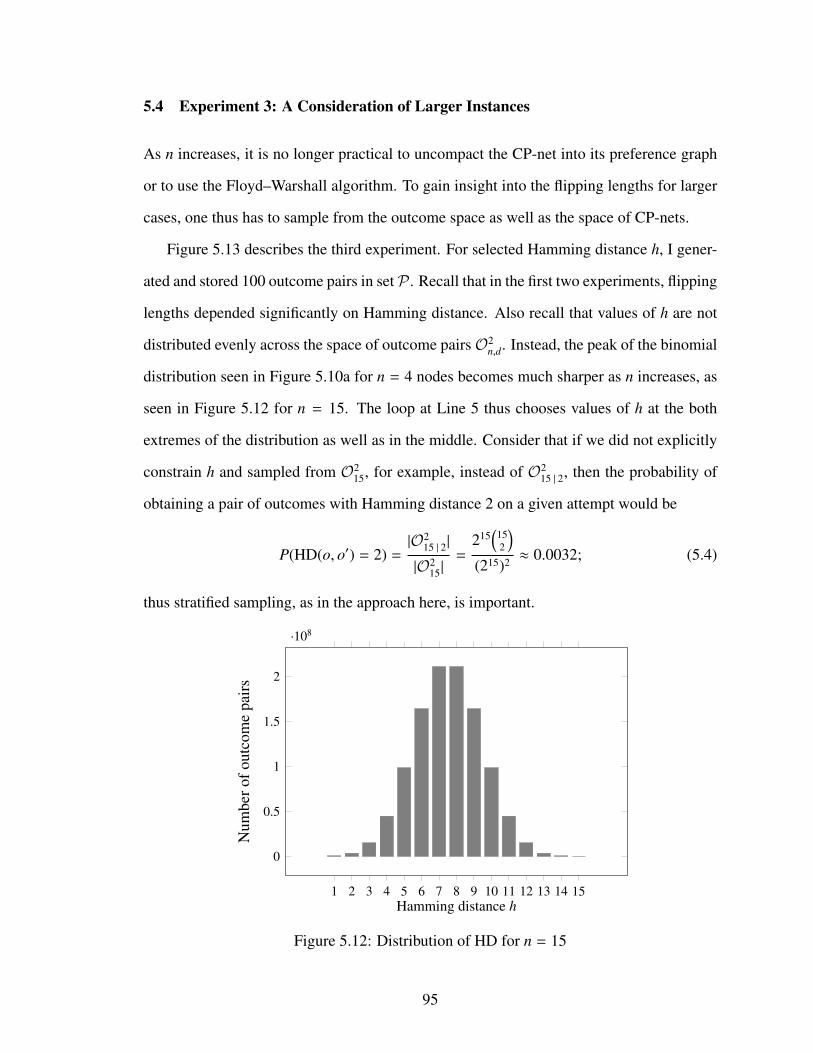
5.4 Experiment 3: A Consideration of Larger Instances
As n increases, it is no longer practical to uncompact the CP-net into its preference graph
or to use the Floyd–Warshall algorithm. To gain insight into the flipping lengths for larger
cases, one thus has to sample from the outcome space as well as the space of CP-nets.
Figure 5.13 describes the third experiment. For selected Hamming distance h, I gener-
ated and stored 100 outcome pairs in set P . Recall that in the first two experiments, flipping
lengths depended significantly on Hamming distance. Also recall that values of h are not
distributed evenly across the space of outcome pairs O2n,d. Instead, the peak of the binomial
distribution seen in Figure 5.10a for n = 4 nodes becomes much sharper as n increases, as
seen in Figure 5.12 for n = 15. The loop at Line 5 thus chooses values of h at the both
extremes of the distribution as well as in the middle. Consider that if we did not explicitly
constrain h and sampled from O215, for example, instead of O2
15 | 2, then the probability of
obtaining a pair of outcomes with Hamming distance 2 on a given attempt would be
P(HD(o, o′) = 2) =|O2
15 | 2|
|O215|
=215
(152
)(215)2 ≈ 0.0032; (5.4)
thus stratified sampling, as in the approach here, is important.
1 2 3 4 5 6 7 8 9 10 11 12 13 14 15
0
0.5
1
1.5
2
·108
Hamming distance h
Num
bero
fout
com
epa
irs
Figure 5.12: Distribution of HD for n = 15
95

Larger-Cases
Output: database consisting of DT instances and flipping lengths
1: initialize database2: d ← 2 . binary domains3: for n← 10 to 15 do . number of features4: P ← ∅5: for h ∈ 2, dn/2e, n do . Hamming distance6: for t ← 1 to 100 do . generate 100 outcome pairs7: P ← P ∪ random outcome pair (o, o′) ∈ O2
n,d | h8: end for9: end for
10: for c← 1 to 4 do . indegree bounded by small constant11: N ← ∅12: for t ← 1 to 100 do . generate 100 CP-nets13: N ← N ∪ Random-CP-net(n, c, d)14: end for15: end for16: for all N ∈ N do . iterate over sampled CP-nets17: for all (o, o′) ∈ P do . iterate over sampled outcome pairs18: ` ← Iterative-DT*(N, o, o′,∞) . compute flipping length19: store (n, c, d, h,N, o, o′, `) in database20: end for21: end for22: end for23: return database
Figure 5.13: Third Experiment: Sample Outcome Pairs and CP-nets
Generate-CP-net is then called to generate 100 CP-nets for each value of n and c as
for the first two experiments. The nested loops at Line 16 and Line 17 iterate over all DT
instances N ×P , such that the same outcome pairs are applied to every CP-net N. Finally,
observe that Line 18 calls Depth-Limited-DT* rather than the Floyd–Warshall algorithm
to perform DT and determine the flipping length for each instance. Depth-Limited-DT*,
adapted from the DT* algorithm of Li et al. [68], is discussed in Section 5.6. Note that
for this experiment the depth limit k is set to ∞ and search continues indefinitely until a
solution is found or the algorithm reports false indicating that no flipping sequence exists
at any depth. I performed a similar experiment for multivalued domains of size d = 3.
96

Table 5.6: Mean Flipping Length Given n, c, and h (Binary Variables, n = 10 to 15)
Hamming distance h = 2
n h c = 1 2 3 410 2 2.75 2.48 2.27 2.3411 2 2.57 2.47 2.42 2.4312 2 2.52 2.40 2.57 2.5213 2 2.44 2.58 2.52 2.5114 2 2.60 2.54 2.58 2.5615 2 2.81 2.38 2.58 2.59
Hamming distance h = dn/2e
n h c = 1 2 3 410 5 6.50 6.47 6.14 5.7911 6 7.82 7.61 7.33 7.0012 6 7.82 8.03 7.62 7.0713 7 9.61 9.19 8.82 8.3814 7 10.21 9.45 8.93 8.4115 8 10.86 10.73 10.01 9.53
Hamming distance h = n
n h c = 1 2 3 410 10 10.00 10.12 10.04 10.0011 11 11.00 11.26 11.08 11.0112 12 12.00 12.32 12.07 12.0113 13 13.00 13.37 13.14 13.0214 14 14.00 14.38 14.10 14.0715 15 15.00 15.39 15.10 15.04
The experiment is the same as shown in Figure 5.13, except that it assigns variable d to
3 in Line 2 and that it specifies in Line 3 that n ranges from 5 to 10 instead of 10 to 15.
Tables 5.6 and 5.7 show results similar to those in the previous experiment for smaller
values of n.
97

Table 5.7: Mean Flipping Length Given n, c, and h (Multivalued Variables d = 3)
Hamming distance h = 2
n h c = 1 2 3 45 2 2.42 2.42 2.37 2.276 2 2.40 2.55 2.45 2.317 2 2.52 2.74 2.54 2.468 2 2.72 2.97 2.62 2.559 2 2.76 2.62 2.66 2.6110 2 2.71 2.78 2.74 2.59
Hamming distance h = dn/2e
n h c = 1 2 3 45 3 3.67 3.66 3.42 3.386 3 3.96 3.80 3.52 3.477 4 5.52 5.47 4.81 4.728 4 5.80 5.71 5.09 4.789 5 7.16 7.08 6.42 5.9710 5 8.37 7.28 6.67 6.19
Hamming distance h = n
n h c = 1 2 3 45 5 5.83 5.64 5.42 5.436 6 7.19 6.80 6.66 6.517 7 8.69 8.16 7.74 7.558 8 10.20 9.41 8.85 8.729 9 11.14 10.65 9.99 9.90
10 10 12.68 11.97 11.13 10.91
98

5.5 Are Preferences Really Transitive?
To this point, we have assumed, except for the brief discussion in Section 1.1.3, that pref-
erences are transitive. That is, if a subject prefers o o′ and o′ o′′, then we reason
that the subject also prefers o o′′. This assumption is the basis for constructing flipping
sequences via the ceteris paribus rules of the CP-net. However, let us briefly reconsider
Peter C. Fishburn’s example [36] from Chapter 1. This time, instead of a long sequence
of cups of coffee, each with one more grain of sugar than its predecessor, consider that we
have a similarly long sequence of beverages described by multiple features, such as sweet-
ness, temperature, provenance, and the presence of varied subtle flavorings. The subject’s
preference over the combinatorial domain is described with a CP-net, and a DT algorithm
assures us that the subject will prefer beverage o to o′ due to very long flipping sequence,
as shown in Figure 5.14. We saw in Sections 5.2–5.4 that flipping sequences much longer
than the Hamming distance are rare. However, sequences of length O(n2) certainly exist
even in binary CP-nets with complete tables, and Boutilier et al. [16] showed that in certain
cases flipping lengths can be exponential in n.
Recall that each flip in the sequence is entailed by a particular CPR. As discussed
in Chapter 1, CP-nets are considered to be a static, deterministic formalism. That is, it is
assumed that for each outcome pair that differs in just one feature, the subject always makes
the same choice. One should keep in mind, however, that this determinism is a modeling
decision, not an intrinsic property of the subject’s underlying preferences. Whether N is
constructed by the subject, elicited through queries, or learned from data in any of the
ways discussed in Sections 1.2.3 and 3.5, it is reasonable to allow for the possibility that
o′ = o0
≺
o1
≺
o2
≺ · · · ≺
o` = o
Figure 5.14: An Exceptionally Long Flipping Sequence
99

Table 5.8: Noise Model for Maximum Reliable Flipping Lengths
Probability of Noise ε Max Flipping Length `0.10% 6920.50% 1381.00% 685.00% 13
the model reflects some margin of error, or noise. If such errors are small, they can be
safely ignored. However, the presence of noise turns out to be particularly problematic for
very long flipping sequences.
Consider that in a flipping sequence, each flip (ot, ot+1) is permitted by a particular CPR
u : i, where ot[i] , ot+1[i], ot[−i] = ot+1[−i], u = o[Pa(Xi)], 1 ≤ i ≤ n, 0 ≤ t < `. Let
ε ∈ (0, 1) be the probability that each CPR in the CP-net is noisy. The probability p that a
particular flipping sequence of length ` entails dominance despite noise is then
p = (1 − ε)` , (5.5)
which converges to 0 as ` tends to infinity.8 Assuming p ≥ 0.5 and solving for ` gives us
` ≤
⌊−1
log2(1 − ε)
⌋. (5.6)
Table 5.8 shows the longest reliable values of ` for varying noise levels ε.
The problem of noise is of course not limited to CP-nets. Any predictive model, if it
admits too much noise, becomes unreliable. The tendency of very long transitive sequences
to accumulate noise, however, is a further reason to limit search depth.
5.6 Depth-Limited Dominance Testing
Sections 5.2–5.5 can be summarized as follows: The deeper the search in DT, the lower
the probability that a path exists, and the higher the probability that the path is unreliable.
It thus seems reasonable in many settings to limit search depth, as we now discuss.8Here I consider only a single flipping sequence from o′ to o. Multiple paths from o′ to o of length ` are
possible, as in Figure 5.2, but this complicates the analysis.
100

Definition 38 (Depth-limited dominance). Let (N, o, o′) be an arbitrary DT instance. For
any positive integer k, N entails the depth-k dominance of o over o′,
N |= o k o′, (5.7)
if and only if FL(N, o′, o) ≤ k. If a flipping sequence of length ` ≤ k exists, then we also
say the first outcome k-dominates the second, and write o k o′.
We call the search for such a sequence depth-limited dominance testing (DLDT). A
general algorithm for conducting DLDT is described in Figure 5.15. The algorithm takes
as its input a DT instance, specified depth limit k, and a reference to a blackbox subroutine
DTSolver that returns true if a path of length ` ≤ k exists and may return unknown if the
cutoff is reached before the search tree is fully explored. The loop in Line 2 iterates over
feasible flipping lengths from ` = HD(o, o′) to k in increments of 2 (see Theorems 34 and
36). The algorithm returns the length ` ≤ k of a flipping sequence from o′ to o, if such a
sequence exists, or∞ if o k o′.
Let us briefly discuss two algorithms that can serve as the DTSolver subroutine. Sec-
tion 5.6.1 shows how to adapt the DT* algorithm proposed by Li et al. [68]. Section 5.6.2
then proposes SAT-DT, a novel approach that solves DT instances of specified flipping
length via reduction to Boolean satisfiability (SAT). The algorithms can easily be adapted
to return the flipping sequence as well if that is desired.
5.6.1 Depth-Limited DT*
DT* employs a heuristic approach to dominance testing. A priority queue is employed,
with a heuristic function on any outcome o* to guide the search. Nodes on the fringe of
the search tree with the lowest positive values of f (o*) are searched first; negative values
of f (o), however, rule out any possibility of finding a solution. Pseudocode, adapted from
Li et al. [68], is provided in Figure 5.16. The boxes emphasize changes that are central to
the iterative approach employed here for DLDT. Note that if the depth limit ` is reached,
101

DLDT( N, o, o′, k, DTSolver )
Input: N CP-neto Goal outcomeo′ Start outcomek Depth limitDTSolver Subroutine to solve depth-limited DT instances
Output: ` Flipping length if sequence found, otherwise∞
1: s← 2 if N is binary valued and 1 otherwise2: for ` ← HD(o, o′) to k step s do . Iterative search depth3: answer← DTSolver (N, o, o′, `) . Invoke subroutine4: if answer = true then5: return ` . Return flipping length ` indicating N |= o ` o′
6: else if answer = false then7: return∞ . No solution exists at any depth, so halt search8: end if9: end for
10: return∞ . No solution with flipping length ` ≤ k
Figure 5.15: Generic Algorithm: Depth-Limited Dominance Testing
no successor nodes in the search tree will be added to the priority queue. If this occurs, the
algorithm returns unknown. If all solutions can be ruled out, it returns false.
5.6.2 DT-SAT
The section concludes with a reduction of DLDT to SAT, as shown in Figure 5.17. For
this reduction outcomes are modeled as states and flips as actions that transition between
states, employing the satisfiability as planning (SATPlan) method of Kautz and Selman
[54]. The variable ω denotes a Boolean formula in Conjunctive Normal Form (CNF),
i.e., a conjunction of clauses, each a disjunction of literals. Initially ω is empty, with an
assumed truth value of true, which we denote with the assignment ω ← >. To write a
clause ξ means to conjoin it to ω to form a new formula, ω ← ω ∧ ξ. When all clauses
have been written thus, a SAT solver is called. It is assumed that the solver returns true if
ω is satisfiable and false otherwise.
102

Depth-Limited DT*( N, o, o′, ` )
Input: N CP-neto Goal outcomeo′ Start outcomek Depth limit
Output: result true if N |= o k o′, false if N |= o′ 6 o; else unknown
1: if f (o′) < 0 then . Heuristic function [68]2: return false3: end if4: cutoff← false5: insert (o′, 0) into priority-queue with priority f (o′)6: while priority-queue , ∅ do7: (o′, ` )← remove-first(priority-queue)8: if o′ = o then . Goal test9: return true
10: end if11: for all Xi ∈ V do12: if improvable(o′, Xi) ∧ Xi < any-matching-suffix(o′, o) then13: o′′ ← single-flip(o′, Xi)14: if not-repeated(o′′) ∧ f (o′′) ≥ 0 then15: if ` ≥ k then . Can we flip and not exceed depth limit?16: cutoff← true . Thus will not search complete graph17: else18: insert (o′′, ` + 1) into priority-queue with priority f (o′′)19: end if20: end if21: end if22: end for23: end while24: if cutoff = true then25: return unknown26: else27: return false28: end if
Figure 5.16: Solver Algorithm: Depth-Limited DT*
103

DT-SAT( N, o, o′, ` )
Input: N CP-neto Goal outcomeo′ Start outcome` Predetermined search depth
Output: Boolean true if N |= o ` o′, otherwise false
1: ω← >2: for i← 1 to n do . Assert initial and final states3: ω← ω ∧ z0,i,o′[i]
4: ω← ω ∧ zt,i,o[i]
5: end for6: for t ← 1 to ` do . Just one state occurs for all t, i7: for i← 1 to n do8: ω← ω ∧ JustOne
1≤ j≤dzt,i, j
9: end for10: end for11: for t ← 1 to ` − 1 do12: for i← 1 to n do13: for distinct i, j ≤ d do14: ω← ω ∧ αt,i, j,k ⇒ zt,i, j ∧ zt+1,i,k . Implications of actions15: for h← 1 to n s.t. h , i do . Framing rules16: for q← 1 to d do17: ω← ω ∧ αt,i, j,k ∧ zt,h,q ⇒ zt+1,h,q
18: ω← ω ∧ αt,i, j,k ∧ ¬zt,h,q ⇒ ¬zt+1,h,q
19: end for20: end for21: end for22: end for23: ω← ω ∧ JustOne
1≤i≤n,1≤ j,k≤dαt,i, j,k
24: for each CPR in N of the form u : xij xi
k do25: ω← ω ∧ zt,p1,u1 ∧ · · · ∧ zt,pm,um ⇒ ¬αt,i, j,k . Disallow flip unless CPR permits26: end for27: end for28: answer← SAT-solver(ω)29: if answer = true then30: return true31: else32: return unknown33: end if
Figure 5.17: Solver Algorithm: DT-SAT
104

States
Let o0, o1, . . . , o`−1, o` be the outcomes in a flipping sequence, such that o′ = o0, o = o`,
HD(ot, ot+1) = 1, ot[i] , ot+1[i], ot[−i] = ot+1[−i], 0 ≤ t < `, 1 ≤ i ≤ n. We denote
by j = ot[i] the value of Xi in the outcome at time t. The outcomes zt,i, j are modeled as
Boolean state variables
zt,i, j ⇐⇒ ot[i] = xij, (5.8)
for all (t, i, j), 0 ≤ t ≤ `, 1 ≤ i ≤ n, 1 ≤ j ≤ d. Clauses are written to assert that the
initial and final states, o′ and o, occur at times 0 and ` respectively. It is also asserted that
a variable Xi can have just one state at time t. That is, the variable has at least one state
(value) and at most one state (value). For this it is helpful to define the operator
JustOne1≤ j≤d
zt,i, j =(zt,i,1 ∨ zt,i,2 ∨ · · · ∨ zt,i,d
)∧
(¬zt,i,1 ∨ ¬zt,i,2
)∧
(¬zt,i,1 ∨ ¬zt,i,3
)...
∧(¬zt,i,1 ∨ ¬zt,i,d
)∧
(¬zt,i,2 ∨ ¬zt,i,3
)...
∧(¬zt,i,d−1 ∨ ¬zt,i,d
)which is used here in a manner analogous to the summation and product operators,
∑and∏
.
Actions
Boolean variables αt,i, j,k are also defined for each possible action. In a flipping sequence
the value of just one variable changes at each time t. Thus, for all t < `, i ≤ n, and distinct
xij, x
ik ∈ Dom(Xi), there is a possible action corresponding to a flip from xi
j to xik. These are
expressed in terms of their implications
αt,i, j,k =⇒ zt,i, j ∧ zt+1,i,k, (5.9)
105

and it is specified that just one action occurs at every timestep t < `. Framing rules are
also written to specify that if an action causes a variable to change, the other n−1 variables
maintain their values from time t to t + 1.
αt,i, j,k ∧ zt,h,q =⇒ zt+1,h,q (5.10)
αt,i, j,k ∧ ¬zt,h,q =⇒ ¬zt+1,h,q (5.11)
Modeling the CPRs
For SATPlan it is more natural to express what action did not occur. The pairwise relation-
ships between domain values in the CPR is thus expressed as a conjunction of actions that
did not occur in a valid flipping sequence of length `.
A rule of the form u : xij xi
k, where u = u1u2 · · · um ∈ Asst(Pa(Xi)), means a flip cannot
occur from xij to xi
k in Xi when that node’s parents are assigned the values in u; hence action
αt,i, j,k cannot occur under such circumstances. Let Xp1 , Xp2 , . . . , Xpm denote the parents of
Xi, such that Xp1 = xp1u1 , Xp2 = xp2
u2 , etc. Observe that at time t in the flipping sequence,
these assignments correspond to the state variables zt,p1,u1 , zt,p2,u2 , etc. Thus, the algorithm
outputs rules of the form
zt,p1,u1 ∧ zt,p2,u2 ∧ · · · ∧ zt,pm,um ⇒ ¬αt,i, j,k. (5.12)
5.7 Conclusion
An oft-cited objection to the use of CP-nets is that the problem of dominance testing, de-
ciding whether one outcome is preferred to another, is NP-hard. Moreover, the proofs of
dominance, so-called flipping lengths, can be exponentially long. In the experiments de-
scribed in this chapter, I have shown that while long sequences exist, they are rarer than
sometimes supposed and tend to occur most often for dependency graphs with long aver-
age path lengths. Expected flipping length also depends on factors such as the number of
variables, maximum indegree of nodes in the dependency graph, domain size, and the Ham-
106

ming distance of the outcomes. I have shown that limiting search depth is often reasonable
and showed how to achieve this by adapting an existing heuristic solver to perform itera-
tively deepening, depth-limited search, as well as through a reduction to SAT to leverage
the heuristics in modern solvers. In future work, I hope to show how to leverage parame-
ters such as average path length and Hamming distance to enable portfolio approaches to
dominance testing.
Copyright c© Thomas E. Allen, 2016.
107

Chapter 6 Local Search for Learning Tree-Shaped CP-nets
This chapter proposes a novel method for learning tree-shaped CP-nets from choice data.
It is sometimes claimed that CP-nets are “easy to elicit” [16]. That is, we explain CP-nets
to the user, and she introspects on her preferences and writes down the CP-net that best de-
scribes her decision-making process when comparing alternatives. This is a fairly common
assumption in the CP-net literature [18, 30]. Psychologists, however, question our ability
to introspect in this way. They point out that people’s reported preferences are often in-
consistent with their choices and, unexpectedly, that introspection about preferences often
decreases the chooser’s satisfaction with their choice [39, 40, 97, 103].
On the other hand, when presented with alternatives, people often do seem to know
what they want, even if they cannot explain the underlying reasoning process in a con-
trolled experiment. Based on this assumption that we can use our preferences without fully
understanding their underlying form, several recent CP-net elicitation algorithms depend
on choice data—sets of binary choices from some domain. Some algorithms assume that
the choices have been made prior to run time [23, 64], a process known as passive learn-
ing. Others adaptively offer alternatives in an effort to decrease the number of queries
needed. Such active learning paradigms include querying the user about their preferences
directly [23, 29, 47] or Angluin-style learning queries [58]. (See Sections 1.2.3 and 3.5.)
Both in psychological experiments and in many preference data sets, such as those in
the PrefLib repository [75], one can find examples of noisy and inconsistent preferences.
For example, Kamishima and Akaho [53] point out that when consumers were asked to
rank ten sushi items and then later to assign rating scores to the same items, in 68% of the
cases, the ordering implied by the ratings did not agree with the ranking elicited directly
only minutes before. There are many explanations for such phenomena, including a lack of
computational power to compute optima consistently, and a very human desire for variety
108

[76]. To our knowledge only Liu et al. [70] have addressed the problem of learning CP-
nets from noisy data. However, their algorithm explicitly builds a preference graph on
the outcomes, which is exponentially larger than the CP-net. The algorithm we present
implicitly represents the preference graph by only constructing the CP-net and is far more
efficient with respect to space.
The approach that we take in this chapter falls into the category of passive learning, in
which the agent unobtrusively records the user’s choices and then fits a CP-net model to
the observed pairwise comparison data. Note that this approach to learning differs from
approaches in which “big data” from large populations are systematically mined in an
effort to predict user behavior. In our case, the data arise, for example, from an individual
for whom we are trying to customize a particular system.
Recall that many problems involving CP-nets and their variants, including learning
a CP-net that is consistent with comparison data (Section 3.5) and using that CP-net to
determine which of two arbitrary outcomes is preferred (Section 3.4), are known to be
computationally hard. However, the dominance problem is known to be easy for CP-nets
for which the dependency structure is a tree. Here we restrict our attention to this subclass
of CP-nets in order to take advantage of efficient dominance testing.
In Section 6.1 we review local search as well as graph theoretic concepts that are needed
to explain our approach. In Section 6.2 we offer a novel encoding for tree-shaped CP-nets
that is useful in defining a neighborhood in which local search can be conducted. In Sec-
tion 6.3 we consider how to evaluate prospective models with respect to a set of possibly
noisy of example data. We discuss the learning algorithm itself in Section 6.4. In Sec-
tion 6.5 we evaluate the algorithm with experiments. A conclusion follows in Section 6.6.
6.1 Background
A tree-shaped CP-net is a conditional preference network (see Definition 9) for which the
dependency graph takes the shape of a directed forest. The term tree in this context is
109

A B C
D E
a aa : b ba : b b
b : c cb : c c
b : d db : d d
c : e ec : e e
(a) CP-net N1 (Connected Digraph)
A B C
D E
a a b b c c
b : d db : d d
c : e ec : e e
(b) CP-net N2 (Disconnected)
Figure 6.1: Tree-shaped CP-nets
potentially confusing, since the digraph may have more than one connected component;
our terminology follows that of Boutilier et al. [16]. Recall from Section 2.2 that a directed
tree is a digraph G = (V, E) such that, for just one node s, called the root, and every other
node t, where s ∈ V, t ∈ V , s , t, there exists just one path from s to t. In contrast, a
directed forest is a digraph in which each node has at most one parent; thus, a directed tree
is also a directed forest, but the converse does not hold. One can observe that the number of
roots is the same as the number of connected components or directed trees that make up the
directed forest. Figure 6.1 depicts two tree-shaped CP-nets, one in which the dependency
graph is a directed tree, the other in which it is a directed forest.
Unless otherwise noted, a CP-net in this chapter is assumed to be tree-shaped. We also
assume here that the domain of each variable is binary and that each conditional preference
table (CPT) of the network is complete, i.e., contains a conditional preference rule (CPR)
for each assignment to the variables that label the node’s parents in the dependency graph,
which in this case will be either a single parent, or the empty set for nodes that are roots.
In this chapter, we represent a directed forest as an undirected tree. A tree, when used
without any modifier, refers to a labeled, undirected graph G = (V, E) in which any two
vertices, u ∈ V , v ∈ V , u, v ∈ E u , v, are connected by just one path. Similarly, a
110

1 2 3
4 5
6
(a) Tree T1
1 2 3
4 5
6
(b) Tree T2
Figure 6.2: Rooted Trees
forest, if not qualified as directed, is a union of disjoint, labeled, undirected trees. We may
distinguish one node of a tree as a root. In that case, the tree is a rooted tree; otherwise,
the tree is assumed to be unrooted. In this chapter, since we work with both directed and
undirected graphs, we will refer to directed graphs as digraphs and to undirected graphs
simply as graphs. Figure 6.2 depicts two rooted trees.
We denote by E = E1, E2, . . . , E` a set of example data. We also refer to these data as
choice data or outcome comparisons. Each element Et = (ot, o′t) of the set is an outcome
pair, ot ∈ O, o′t ∈ O, in which the first element is preferred to the second, i.e., ot o′t , for
all t, 1 ≤ t ≤ `. Such data are intended as a model of the observed choices of an individual
user over discrete time t. In general such data may be inconsistent; that is, the transitive
closure of E may result in a cycle in which some outcome o is seen to be preferred to itself.
When we say our goal is to learn a CP-net from data E , we mean that we want to
identify, from among a set of models N , one that is most consistent with, or best explains,
E , as described in Section 6.3. Since in general it is infeasible to search the whole space of
|N |models, we will rely on a heuristic approach known as local search, in which the fitness
f (N) of a proposed model N is compared with that of its neighbors, Neigh(N), as discussed
in Section 6.4. The term neighborhood refers to the set of models Neigh(N) ∪ N. If a
model is as fit as any model in its neighborhood, i.e., f (N) ≥ f (N′) for all N′ ∈ Neigh(N),
111

then we say that it is locally optimal. If a model is as fit as any model in N , it is furthermore
a global optimum. If two or more neighbors are equally fit and are as fit as their respective
neighbors, we say they belong to a plateau. For further discussion of local search, the
reader is referred to a textbook such as that of Russell and Norvig [91].
The GSAT [95] and WalkSAT [96] algorithms for Boolean satisfiability serve as inspi-
rations for the method that we describe in Section 6.4. We are not aware of any previous
work applying local search to CP-nets or related formalisms. Various methods for learning
CP-nets are discussed in Section 3.5. The three algorithms that are most relevant to the
problem that we describe here are those of Dimopoulos et al. [29], which assumes that
example data are consistent and reports failure if no model satisfies E ; of Liu et al. [70],
which like ours identifies optima in the presence of possibly noisy examples, but requires
exponential space, since it explicitly constructs the preference graph while our method ex-
tends to larger problem instances; and finally of Bigot et al. [12], which discusses how to
learn tree-shaped probabilistic conditional preference networks (PCP-nets) from optimal
outcomes, while our method learns a deterministic model from pairwise comparison data.
6.2 Encoding Tree-shaped CP-nets
In Section 4.3 we showed how to encode acyclic dependency graphs as dagcodes. For tree-
shaped CP-nets, however, a simpler encoding is available that facilitates local search by
making it more straightforward to define neighbors. Notice that the dependency graph G =
(V, E) of a so-called tree-shaped CP-net is equivalent to a forest GF of undirected, labeled,
rooted trees. To obtain G from GF , in particular the directions of each edge (Xh, Xi) ∈ E,
one need only traverse each tree in GF from its root. Furthermore, one may notice that
there is a nice correspondence between trees and forests of rooted trees: Any forest with n
nodes can be mapped to an equivalent tree with n + 1 nodes by introducing a new node, r,
inserting edges from r to the root of each tree in forest GF , and distinguishing r as the root
of the newly formed tree with n + 1 nodes. Conversely, to recover the forest from the tree,
112

one can simply remove the root and its edges. Observe that trees T1 and T2 in Figure 6.2
correspond to the dependency graphs of N1 and N2 in Figure 6.1 according to this mapping.
Once the digraph of a tree-shaped CP-net with n nodes has been modeled as a tree with
n + 1 nodes, it can be further modeled as a vector of integers known as a Prufer code.1 As
Arthur Cayley proved in the 1800s, for every integer k, the number of unrooted trees with
k labeled nodes is kk−2. Heinz Prufer later showed how to encode each such instance as a
sequence of k − 2 integers that has come to be known as a Prufer code: L = 〈L1, . . . , Lk−2〉,
where L j ∈ 1, . . . , k, 1 ≤ j ≤ k − 2. Any unrooted labeled tree T can be mapped to its
corresponding Prufer code L, and vice versa, by straightforward algorithms that we present
in Figures 6.3 and 6.4, which closely follow Kreher and Stinson [60, 3.3].
To encode the CPTs, we could of course use the mapping described in Section 4.4.
Again, however, a simpler mapping is available since we are dealing with tree-shaped CP-
nets with binary variables. Recall from Equation 4.3 that the number of non-degenerate
CPTs of a node with m parents is
ψ2(m) =
m∑k=0
(−1)m−k
(mk
)22k. (4.3 revisited)
Moreover, since each node has at most 1 parent, Equation 4.3 evaluates to
ψ2(0) = ψ2(1) = 2 (6.1)
for every CPT of a tree-shaped CP-net composed of binary variables.2 We can thus rep-
resent the CPTs of a tree-shaped CP-net as a vector B of n integers B[i] = 0 or B[i] = 1,
1 ≤ i ≤ n, according to the mapping
xi xi B[i] = 0
xi xi B[i] = 1(6.2)
1Note that a Prufer code of a tree with n nodes consists of n − 2 integers, each ranging from 1 to n.There are thus nn−2 trees on n labeled nodes. However, since the tree-shaped dependency graphs describedby Boutilier et al. [16] actually correspond to forests (!), we have to add an additional node n + 1 to therepresentation. Thus, in the case of so-called tree-shaped CP-nets, the corresponding Prufer code actuallyconsists of n − 1 integers ranging from 1 to n + 1.
2Note that ψd(0) , ψd(1) for d > 2.
113

Tree-to-Prufer-Code( E, n )
Input: E undirected edges of the treen number of labeled nodes
Output: L Prufer code consisting of n − 2 integers
1: d ← 0 vector of length n2: for all j, k ∈ E do . compute the degrees d of the n nodes3: d[ j]← d[ j] + 14: d[k]← d[k] + 15: end for6: for i← 1 to n − 2 do . on ith iteration we have a tree on n + 1 − i nodes7: j← n8: while d[ j] , 1 do . find j, the largest labeled node of degree 19: j← j − 1
10: end while11: k ← n12: while j, k < E do . find edge j, k ∈ E13: k ← k − 114: end while15: L[i]← k . store label k in code16: d[ j]← d[ j] − 1 . reduce the degrees j and k17: d[k]← d[k] − 118: E ← E \ j, k . and delete that edge19: end for20: return L = 〈L[i], . . . , L[n − 2]〉
Figure 6.3: Algorithm: Tree to Prufer Code [60]
for each node Xi with no parents and
xh : xi xi
xh : xi xiB[i] = 0
xh : xi xi
xh : xi xiB[i] = 1
(6.3)
for each remaining node Xi with a single parent Xh, Xh ∈ V , Xi ∈ V , 1 ≤ h ≤ n, 1 ≤ i ≤ n.
By combining the encodings for the digraph and CPTs, it is possible to model every
tree-shaped CP-net N as a treecode (L, B) consisting of a Prufer code L with n − 1 integers
L j ∈ 1, . . . , n + 1, 1 ≤ j ≤ n − 1, for the dependency graph, and a bit vector B with n
bits for the CPTs. The algorithms of Figures 6.5 and 6.6 show how to map an arbitrary
114

Prufer-Code-to-Tree( L, n )
Input: L Prufer code consisting of n − 2 integersn eventual number of labeled nodes
Output: E directed edges composing the tree
1: E ← ∅2: L[n − 1]← 13: d ← vector of n 1s4: for i← 1 to n − 2 do . compute degrees from L5: d[L[i]]← d[L[i]] + 16: end for7: for i← 1 to n − 1 do8: j← n9: while d[ j] , 1 do . find j, the largest labeled node of degree 1
10: j← j − 111: end while12: k ← L[i]13: d[ j]← d[ j] − 1 . reduce the degrees of j and k in L14: d[k]← d[k] − 115: E ← E ∪ j, k . insert the edge into E16: end for17: return E
Figure 6.4: Algorithm: Prufer Code to Tree [60]
tree-shaped CP-net N to its corresponding treecode (L, B), and vice versa. Also, Figure 6.7
completes the examples in Figures 6.1 and 6.2 by supplying the corresponding treecodes.
In the theorems and proofs that follow, we denote by TNn the set of all complete tree-
shaped CP-nets on n binary variables and by Tn the corresponding set of treecodes
Tn = Ln × Bn, (6.4)
where Ln denotes the set of all Prufer codes L = 〈L1, . . . , Ln−1〉 with n − 1 integers ranging
from 1 to n + 1 and Bn is the set of all bit vectors B = 〈B1, . . . , Bn〉 with n bits Bi ∈ 0, 1.
We denote by TC : TNn → Tn the function mapping tree-shaped CP-nets to treecodes, as
implemented by Tree-CP-net-to-Treecode as shown in Figure 6.5.
The algorithms presented in Figures 6.5 and 6.6 map treecodes to CP-nets, and vice-
versa, suggesting that the algorithms are inverses. We now formalize this relationship.
115

Tree-CP-net-to-Treecode( N )
Input: N Tree-shaped CP-net with binary variablesOutput: L Prufer code encoding the digraph
B Bit vector encoding the CPTs
1: for i← 1 to n do2: B[i]← 0 or 1 based on mapping in (6.2) and (6.3)3: end for4: relabel nodes V in N with the integers 1 to n5: R← nodes of digraph G of N that are roots6: V ← V ∪ n + 17: E ← E ∪ (n + 1, r) for all r ∈ R8: make edges E undirected9: L← Tree-to-Prufer-Code( E, n + 1 ) . Figure 6.3
10: return (L, B)
Figure 6.5: Algorithm: Tree-shaped CP-net to Treecode
Treecode-to-Tree-CP-net( L, B )
Input: L Prufer codeB Bit vector encoding the CPTs
Output: N Tree-shaped CP-net
1: n← length of B2: assert that L has length n − 13: V ← 1, . . . , n + 14: E ← Prufer-Code-to-Tree(L, n) . Figure 6.45: G = (V, E)6: traverse G from node n + 1 assigning directions to edges in order of traversal7: V ← V \ n + 1 . delete node n + 1 and its edges8: E ← E \ (n + 1, k) for all (n + 1, k) ∈ E9: initialize CP-net N with digraph G
10: obtain CPTs of N from B using mapping in (6.2) and (6.3)11: return N
Figure 6.6: Algorithm: Treecode to Tree-shaped CP-net
116

T1 =
1 3 2 2︸ ︷︷ ︸
LPrufer code for N1
1 0 0 1 1︸ ︷︷ ︸B
CPTs for N1
T2 =
3 2 6 6︸ ︷︷ ︸
LPrufer code for N2
1 0 0 1 1︸ ︷︷ ︸B
CPTs for N2
Figure 6.7: Treecodes Corresponding to the Tree-shaped CP-nets in Figure 6.1
Theorem 39 (Treecode Bijection). TC is a bijection.
Proof. Let N and N′ denote arbitrary tree-shaped CP-nets on n binary variables, where
N ∈ TNn, N′ ∈ TNn, n > 0.
Suppose TC(N) = TC(N′). If so, N and N′ must have the same Prufer code L, hence
the same digraph G. They also must have the same bit vector B; hence, the CPTs of N and
N′ must also be the same for each node. Thus, N = N′.
Next, let T be an arbitrary treecode in Tn. Recall that for every Prufer code L =
〈L1, . . . , Ln−1〉, where L j ∈ 1, . . . , n + 1, 1 ≤ i ≤ n, there exists a labeled, unrooted
tree with n + 1 nodes with labels V = 1, . . . , n + 1. Since n > 0, there exists a unique node
with largest label n + 1. The graph, as a tree, must be connected and free of cycles, so we
will always be able to traverse it from node n + 1 to every other node, applying directions
to each edge in the direction of traversal. We can then delete node n + 1 along with its
edges. Consider that the resulting digraph will be a directed forest that can serve as the
dependency graph G of a tree-shaped CP-net N. Furthermore, by relabeling each node i as
Xi and specifying that Dom(Xi) = xi, xi, 1 ≤ i ≤ n, the digraph will be in its canonical
form. Further consider that once digraph G is available, we will know the parent, if any,
of each node Xi, allowing us to obtain its non-degenerate CPT from Bi via the mapping in
117

Table 6.1: Number of Tree-Shaped CP-Nets (Respectively Treecodes) with n Binary Nodes
n |Tn|
1 22 123 1284 20005 414726 10756487 335544328 12244400649 51200000000
10 2414538435584
Equations 6.2 and 6.3. It follows that for all T = (L, B), T ∈ Tn, L ∈ Ln, B ∈ Bn, n > 0,
there exists N ∈ TN such that TC(N) = T .
Therefore, tree-shaped CP-nets are in one-to-one correspond with treecodes. q
Theorem 40 (Number of Tree-shaped CP-nets). For every non-negative integer n, the num-
ber of tree-shaped CP-nets of n binary variables is
∣∣∣TNn
∣∣∣ = 2n(n + 1)n−1. (6.5)
Proof. The set of treecodes Tn consists of all combinations Ln × Bn. Thus, |Tn| = |Ln||Bn|.
Since a Prufer code L ∈ Ln consists of n − 1 integers ranging from 1 to n + 1 inclusive,
|Ln| = (n + 1)n−1. Also, there are |Bn| = 2n bit vectors of length n. We have already shown
that TNn and Tn are in one-to-one correspondence. Therefore, |TNn| = 2n(n + 1)n−1. q
Table 6.1 gives the computed value of Equation 6.5 for n = 1 to 10 (also see Sloane [98,
A097629]). Note that, as expected, the values are identical to the number of acyclic CP-nets
with n binary variables and bound 1 on indegree, an,1,2 (see Theorem 30 in Section 4.4).
With the help of the encoding and bijection, it is then straightforward to generate all
tree-shaped CP-nets on n binary variables, as illustrated by the pseudocode in Figure 6.8.
118

All-Tree-Shaped-CP-nets( n )
Input: n Number of binary variablesOutput: N Set of all tree-shaped CP-nets
1: N ← ∅2: L← vector of n − 1 1s . first treecode lexicographically3: B← vector of n 0s4: first← (L, B)5: repeat6: N ← Treecode-to-Tree-CP-net(L, B)7: N ← N ∪ N8: (L, B)← Next-Treecode-Lexicographically(L, B, n) . see pseudocode below9: until (L, B) = first . when the figurative odometer finally rolls over
10: return N
Next-Treecode-Lexicographically( L, B, n )
Input: L Prufer code of length n − 1B bit vector of length nn positive integer corresponding to the number of variables
Output: (L, B) Next treecode according to lexicographic order
1: k ← n . start with rightmost bit of B2: while k > 0 do3: B[k]← B[k] + 1 . increment binary digit4: if B[k] < 2 then . and carry if necessary5: break6: end if7: B[k]← 08: k ← k − 1 . move on to the next most significant digit9: end while
10: if B is the 0 vector then . we reached all 1s and rolled over, so now get next L11: k ← n − 112: while k > 0 do13: L[k]← L[k] + 1 . increment (d + 1)-ary digit14: if L[k] < n + 2 then . and carry if necessary15: break16: end if17: L[k]← 1 . Prufer code elements start at 1 not 018: k ← k − 1 . move on to the next most significant digit19: end while20: end if21: return (L, B)
Figure 6.8: Algorithm: Generate All Tree-Shaped CP-nets
119

Random-Treecode( n )
Input: n Number of binary variablesOutput: T Random Treecode in Tn
1: initialize vectors L and B to respective lengths n − 1 and n2: for j← 1 to n − 1 do . generate Prufer code L3: L[k]← element drawn uniformly randomly from 1, . . . , n + 14: end for5: for j← 1 to n do . generate bit vector B6: B[k]← element drawn uniformly randomly from 0, 17: end for8: return (L, B)
Figure 6.9: Algorithm: Generate Random Tree-Shaped CP-net
The strategy is to order the treecodes lexicographically. In this lexicographic ordering, we
first compare the Prufer code L. If the two Prufer codes are the same, then we compare the
bit vectors B. In each case we first compare the first element of the vector. If it is the same,
we move on to the second, and so on, until we reach the end of the vector. Generating all
treecodes is then equivalent to generating all mixed-radix numerals, as discussed in Knuth
[57, 7.2.1.1]. As each successive treecode is generated in this manner, we call Treecode-
to-Tree-CP-net (Figure 6.6) to obtain the corresponding CP-net and add it to the set to be
returned. After generating all (n + 1)n−12n treecodes, (L, B) will “roll back over” to the first
treecode in the lexicographic ordering in Line 9, not unlike an odometer, and the algorithm
will terminate, returning TNn
We can also generate random treecodes (hence random tree-shaped CP-net models)
uniformly with respect to TNn, as shown in Figure 6.9. Note that since we can choose each
element of L and B independently from their respective ranges 1, . . . , n + 1 and 0, 1,
the resulting instances are provably uniform to the extent that we can generate integers
uniformly at random.
120

6.3 Evaluating a Learned Model
A natural idea in discussing CP-net learning is to start with a CP-net NT (a training model)
and generate from it a set of outcome comparisons E =(o1, o′1), (o2, o′2), . . . , (o`, o′`)
such
that the training model entails every example, i.e., NT |= ot o′t for all t, 1 ≤ t ≤ `. The
idea is then to attempt to learn a CP-net NL that recovers the original, such that NL = NT ,
or, if the set of examples is too limited, at least to find a CP-net that entails all of the
comparisons in E .
This approach suffers from two significant problems. First, it assumes that all compar-
isons are entailed by a CP-net. Significantly, this conflicts with the assumption, common
in economics, that preferences arise from an underlying utility function u : O → R. In
that case, every pair of outcomes is comparable provided their respective utilities can be
computed: if u(o) ≥ u(o′), then o o′. Recall that CP-nets, in contrast, induce a partial
order on O; thus, in general, some pairs of outcomes will be incomparable with respect to
the CP-net, N |= o ‖ o′. Rather than trying to recover some presupposed ideal CP-net or
to learn a model that entails every comparison, a more sophisticated approach, as argued
by Lang and Mengin [65, 66], is to find a model that is consistent with every comparison.
(See also the discussion in Section 3.5.)
Since this point often seems to be misunderstood, we offer an example. Suppose there
are 3 variables with values 0 and 1; i.e., Dom(Xi) = 0, 1, Xi ∈ X1, X2, X3. Further
suppose that the user’s preferences on the outcomes arise from the utility function
u(o) =
n∑i=1
2o[n−i−1]. (6.6)
We can then see that
000 ≺ 001 ≺ 010 ≺ 011 ≺ 100 ≺ 101 ≺ 110 ≺ 111. (6.7)
From this we could construct E consisting of all∣∣∣O2
3
∣∣∣ = 28 pairwise comparisons, such that
u(o) > u(o′) =⇒ o o′. However, through exhaustive analysis, it can be shown that there
121

is no tree-shaped CP-net on V , indeed, no CP-net on V , that entails all 28 comparisons.3
Nevertheless, consider that the CP-net N0
X1 X2 X3
1 0 1 0 1 0
while it does not entail (agree with) all of the comparisons, at least does not disagree with
any of them; i.e., for all (o, o′) ∈ E , N0 6|= o′ o. In this sense, N0 can be said to be
consistent with E , although no CP-net entails every example in E .
Second, the notion of learning as recovering an original CP-net or entailing all examples
fails to account for the possibility of noise. Suppose the preferences of a particular user did
in fact arise from CP-net N0, shown above. Suppose that each day, the user must choose
between a pair of distinct outcomes, o and o′, drawn from the set 000 to 111 inclusive. His
observed choices from Monday through Thursday are
Et=4 = (101, 100), (111, 101), (111, 011), (100, 000) . (6.8)
Note that every choice is consistent with CP-net N0. On Friday, he is again asked to choose
between 100 and 101, the same two outcomes he was given on Monday. His preference
has not changed; he still prefers 101 100 on account of CPT(X1). However, he picks 100
by mistake. The system dutifully adds (100, 101) to the data to obtain
Et=5 = (101, 100), (111, 101), (111, 011), (100, 000), (100, 101) . (6.9)
Observe that the resulting preference order is no longer consistent, since 101 100 101.
Thus, there is no possibility of finding a CP-net, or for that matter a deterministic utility
function, that is consistent with every example in E .
This suggests the idea of framing CP-net learning as an optimization problem: Can
we identify a model that maximizes agreement with example data? Provided we have an3Of course, one could define a variable for which the domain contained all 8 values, 000 to 111. The
total ordering can then be entailed by a CP-net with a single node, but in that case no CP-net is needed.
122

objective function f to assess the fitness of a model N with respect to the example data, the
learning problem can be stated as
N* = arg maxN
f (N, E) . (6.10)
Many different notions of fitness (optimality) could be considered for the objective
function. For this chapter, we use a simple one, as follows. Let agree denote the examples
for which the CP-net model entails the same ordering as in E ; Conversely, let disagree
denote those for which the model entails the opposite ordering,
agree = (o, o′) : (o, o′) ∈ E ∧ N |= o o′ (6.11)
disagree = (o, o′) : (o, o′) ∈ E ∧ N |= o′ o , (6.12)
computed by applying dominance testing to each element in E . Given a non-empty set of
example comparisons E , we define the fitness (score) of a prospective model N as
f (N, E) =|agree| − |disagree|
|E |. (6.13)
Note that if (o, o′) ∈ E and N |= o ‖ o′, the pair (o, o′) is not included in either agree or
disagree, but nevertheless reduces the fitness score, which in general can range between -1
and 1 inclusive. To complete the examples given above, the fitness of N0 on all pairs of the
ordering given in Equation 6.7 is (12− 0)/28 ≈ 0.4286. The fitness scores of N0 for Et=4 in
Equation 6.8 and Et=5 in Equation 6.9 are (4 − 0)/4 = 1 and (4 − 1)/5 = 0.6, respectively.
6.4 Learning via Local Search
A chief advantage of the encoding described in Section 6.2 is that it provides a straightfor-
ward way to define neighbors for local search. A pair of tree-shaped CP-nets are neighbors
if their corresponding treecodes differ in just one element. Formally,
Neigh(N) =
N′ : HD(TC(N), TC(N′)
)= 1, N′ ∈ TN
. (6.14)
123
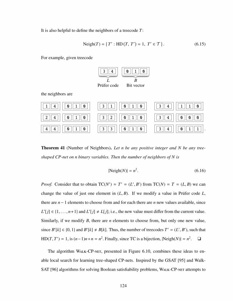
It is also helpful to define the neighbors of a treecode T :
Neigh(T ) =T ′ : HD
(T, T ′
)= 1, T ′ ∈ T
. (6.15)
For example, given treecode
3 4︸ ︷︷ ︸L
Prufer code
0 1 0︸ ︷︷ ︸B
Bit vector
the neighbors are
1 4 0 1 0 3 1 0 1 0 3 4 1 1 0
2 4 0 1 0 3 2 0 1 0 3 4 0 0 0
4 4 0 1 0 3 3 0 1 0 3 4 0 1 1 .
Theorem 41 (Number of Neighbors). Let n be any positive integer and N be any tree-
shaped CP-net on n binary variables. Then the number of neighbors of N is
|Neigh(N)| = n2. (6.16)
Proof. Consider that to obtain TC(N′) = T ′ = (L′, B′) from TC(N) = T = (L, B) we can
change the value of just one element in (L, B). If we modify a value in Prufer code L,
there are n−1 elements to choose from and for each there are n new values available, since
L′[ j] ∈ 1, . . . , n+1 and L′[ j] , L[ j]; i.e., the new value must differ from the current value.
Similarly, if we modify B, there are n elements to choose from, but only one new value,
since B′[k] ∈ 0, 1 and B′[k] , B[k]. Thus, the number of treecodes T ′ = (L′, B′), such that
HD(T,T ′) = 1, is (n−1)n+n = n2. Finally, since TC is a bijection, |Neigh(N)| = n2. q
The algorithm Walk-CP-net, presented in Figure 6.10, combines these ideas to en-
able local search for learning tree-shaped CP-nets. Inspired by the GSAT [95] and Walk-
SAT [96] algorithms for solving Boolean satisfiability problems, Walk-CP-net attempts to
124

Walk-CP-net( E , n, π, max-strikes, max-restarts )
Input: E Example datan Number of variablesπ Probability of taking a random walkmax-strikes Counter to help detect plateauxmax-restarts Limit of random restarts before algorithm terminates
Output: N* Fittest tree-shaped CP-net encountered
1: N*← null model N⊥ with fitness score f (N⊥, · ) = −∞
2: for restarts← 1 to max-restarts do3: N ← Treecode-to-Tree-CP-net(Random-Treecode(n)) . Figures 6.6, 6.94: strikes← 05: repeat6: if f (N, E) > f (N*, E) then7: N*← N . The new model is also the new best model8: strikes← 0 . New height reached, so also reset counter9: if f (N*, E) = 1 then
10: return N* . N* entails all examples, hence also globally best11: end if12: end if13: if random value in [0, 1] ≤ π then14: N ← random element of Neigh(N) . Random walk15: else16: previous-fitness← f (N, E)
17: N ← arg maxN′
f (N′, E) s.t. N′ ∈ Neigh(N)) . Hill climbing
18: if f (N, E) ≤ previous-fitness then . Possible plateau19: strikes← strikes + 120: end if21: end if22: until strikes = max-strikes . Random restart to get off plateau23: end for24: return N* . Give up and return the best model encountered
Figure 6.10: Algorithm: Walk-CP-net
125

find a balance between random and greedy behavior. The algorithm starts by generating a
random model. By default it is the best model yet encountered, so we distinguish it as N*.
With probability π, a user-selected parameter in the range [0, 1], the algorithm then either
randomly walks (Line 14) or attempts hill-climbing (Line 17). In the case of a random
walk, the algorithm replaces N with a randomly selected neighbor. In the case of greedy
behavior, the algorithm performs dominance testing (DT) on E to evaluate all n2 neighbors.
However, while DT is NP-hard for CP-nets in general, it is easy for tree-shaped CP-nets on
binary variables, the class of models that we consider here.
If hill climbing is possible, Walk-CP-net chooses a neighbor with the highest score.
Note that if N is locally optimal, the fitness level may stay the same or even decrease. In
that case, it is possible that the search has reached a plateau. To avoid becoming stranded
there, the algorithm increments a strikes counter. However, if fitness is strictly better, and
the new model turns out to be the best yet encountered, the counter is reset to 0 in Line 8.
When the counter eventually reaches max-strikes, a user-selected parameter, the al-
gorithm performs a random restart, choosing a (potentially distant) model uniformly at
random. The number of random restarts is also controlled by a user-selected parameter,
max-restarts. When this limit is also eventually reached, the algorithm terminates, return-
ing N*, the best model encountered. The algorithm can also terminate early, in Line 10, if
it encounters a model that entails all examples in E . In that case, N* is provably a global
optimum, so we halt the search.
6.5 Experiments
As discussed in Section 3.6, real-world data relevant to CP-nets are in short supply, and the
datasets that are occasionally used for CP-net learning are problematic. Thus, as with most
research involving CP-nets, we used synthetic data to evaluate our algorithm. Figure 6.11
describes how the choice data E are generated. The algorithm first generates an archetypal
tree-shaped CP-net NT uniformly at random. DT is then employed to identify pairs in O2n
126

Generate-Choice-Data( n, `, p, q )
Input: n Number of binary variables` Number of comparisons to return; i.e., |E | ≈ `p Probability of answering o o′ or o′ o randomly when o ‖ o′
q Probability of answering incorrectly; i.e., o′ o when actually o o′
Output: E Example data with ` comparisons specifying o o′ for all (o, o′) ∈ ENT Tree-shaped CP-net used to generate E
1: NT ← Treecode-to-Tree-CP-net(Random-Treecode(n))2: for all o ∈ On or subset of On of size
⌊√`⌋
do
3: for all o′ ∈ On or subset of size⌈√`⌉
such that o , o′ do4: if NT |= o o′ then . model specifies o o′
5: u← o6: v← o′
7: else if NT |= o′ o then . model specifies o′ o8: u← o′
9: v← o10: else . model specifies o ‖ o′
11: x← uniform random number in [0, 1]12: if x < p/2 then . With probability p, we flip a coin,13: u← o . to choose between o o′
14: v← o′
15: else if x < p then16: u← o′ . and o′ o.17: v← o18: else19: continue . The rest of the time, we do not give any answer if o ‖ o′.20: end if21: end if22: y← uniform random number in [0, 1]23: if y < q then . With probability q24: E ← E ∪ (v, u) . answer differently than expected.25: else26: E ← E ∪ (u, v) . The rest of the time, answer as intended.27: end if28: end for29: end for30: E ← random sample of size ` selected uniformly from E31: return (E ,N)
Figure 6.11: Algorithm: Generate Choice Data
127

for which NT entails a preference. When feasible, we iterate over all pairs of outcomes.
When |O2n | is too large, we specify some number ` of outcome pairs to be selected from O2
n
at random.
DT is applied to each resulting problem instance (NT , o, o′) to determine an ordering,
if one exists. If the CP-net does not entail an ordering, i.e., if o ‖ o′, then by default
the algorithm does not include the pair in E . However, this behavior can be customized
by setting a user-specified parameter p. With probability p ∈ [0, 1], when NT |= o ‖ o′,
the algorithm will guess o o′ or o′ o at random. (The rest of the time, i.e., with
probability 1− p, the algorithm does not report a preference for pairs that are incomparable
with respect to NT .) This behavior is analogous to that of a subject who sometimes has to
choose between two outcomes even though he has little information to indicate which is
better. Note, however, that choosing in this randomized manner introduces noise into the
choice data, since if p > 0, the resulting transitive closure of E is likely to contain a cycle.
Noise can also be introduced via a separate parameter, q. With probability q ∈ [0, 1], the
algorithm will misreport the preference, analogous to a subject who on occasion makes an
incorrect choice. Again, note that even small, non-zero values of q are likely to cause E to
be inconsistent. While it is possible to specify non-zero values of p and q simultaneously,
we did not do this for our experiments.
For the first experiment, we generated an original CP-net NT on n = 4 variables. The
choice data E consisted of all pairs (out of 120 possible) for which the original CP-net
entailed a preference. We generated 100 such datasets and ran the Walk-CP-net learning
algorithm on the data multiple times to compare the performance of each learned model
to that of the original model NT . Since no noise was introduced into the example data,
the original model always had a fitness score of 1.0. We ran the learning algorithm 100
times for each of the 100 data sets, varying the max-restarts parameter. The bar chart
in Figure 6.12 shows the mean fitness score achieved for 10, 50, 100, and 500 restarts,
respectively.
128

5 10 50 100 5000
0.2
0.4
0.6
0.8
1
0.680.74
0.870.91
0.99
Maximum Number of Restarts
Mea
nFi
tnes
sR
elat
ive
toO
rigi
nalC
P-ne
t
Figure 6.12: Walk-CP-net Experiment 1 (No Noise)
For the second experiment, we used parameter p to introduce varying degrees of noise.
Note that once noise is introduced, it is possible—in fact, likely—that some tree-shaped
CP-net N* other than the original CP-net NT offers a better fit to E . To provide an ora-
cle for the learning problem, we thus used the algorithm Find-Best-Tree-Shaped-CP-net
shown in Figure 6.13. The oracle iterates over all N ∈ TNn tree-shaped CP-nets to find a
model that has maximum fitness with respect to E . The learned model NL is then com-
pared to the model obtained from the oracle rather than to the original or the one selected
by the oracle. Note that when too much noise is introduced, it is often the case that no
model performs well, including the original. We generated 100 datasets with noise level
p = 0.02 and ran the learning algorithm 100 times on each, again varying the max-restarts
parameter. The bar chart in Figure 6.14 shows the mean fitness score achieved relative to
the oracle for 10, 50, 100, and 500 restarts, respectively.
129
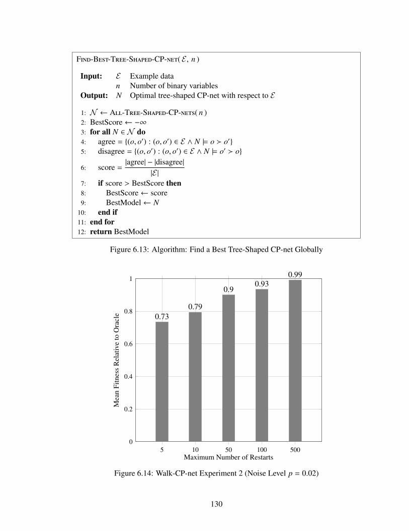
Find-Best-Tree-Shaped-CP-net( E , n )
Input: E Example datan Number of binary variables
Output: N Optimal tree-shaped CP-net with respect to E
1: N ← All-Tree-Shaped-CP-nets( n )2: BestScore← −∞3: for all N ∈ N do4: agree = (o, o′) : (o, o′) ∈ E ∧ N |= o o′5: disagree = (o, o′) : (o, o′) ∈ E ∧ N |= o′ o
6: score =|agree| − |disagree|
|E |7: if score > BestScore then8: BestScore← score9: BestModel← N
10: end if11: end for12: return BestModel
Figure 6.13: Algorithm: Find a Best Tree-Shaped CP-net Globally
5 10 50 100 5000
0.2
0.4
0.6
0.8
1
0.730.79
0.90.93
0.99
Maximum Number of Restarts
Mea
nFi
tnes
sR
elat
ive
toO
racl
e
Figure 6.14: Walk-CP-net Experiment 2 (Noise Level p = 0.02)
130

The third experiment was similar to the second, except that we set noise parameter q,
rather than p. That is, rather than randomly “guessing” an ordering for some incomparable
pairs of outcomes, the answer for an entailed pair of outcomes is reversed with probability
q. The bar chart in Figure 6.15 shows the mean fitness score achieved relative to the oracle
for q = 0.03. Keep in mind that the comparison metric is the fitness score relative to the
oracle for each generated data set E , and that when example data are noisy, even the oracle
usually achieves a fitness score less than 1.0.
Finally, we generated larger problem instances (Table 6.2). Since consulting the oracle
was infeasible for these, we did not include noise. For this experiment we generated tree-
shaped CP-nets with 10, 15, and 20 nodes, with 100 CP-nets in each set. For each CP-net,
we generated a choice set E consisting of 45 comparisons entailed by the original CP-net.
We then repeatedly ran Walk-CP-net for each of the 100 datasets, increasing the maximum
number of restarts by about 50% on each iteration. We continued this until we reached a
5 10 50 100 5000
0.2
0.4
0.6
0.8
1
0.740.81
0.920.96
1
Maximum Number of Restarts
Mea
nFi
tnes
sR
elat
ive
toO
racl
e
Figure 6.15: Walk-CP-net Experiment 3 (Noise Level q = 0.03)
131

Table 6.2: Walk-CP-net Experiment 4 (No Noise)
Variables Restarts Mean Fitness Mean DT Calls†
10 10 0.86 410 15 0.89 810 22 0.92 1410 33 0.94 2510 49 0.95 43
15 10 0.77 915 15 0.80 1615 22 0.83 2915 33 0.85 5215 49 0.87 8915 73 0.88 14915 109 0.90 25015 163 0.92 41015 244 0.93 67015 366 0.94 109015 549 0.95 1762
20 10 0.72 1420 15 0.75 2720 22 0.77 4920 33 0.80 8820 49 0.82 15120 73 0.83 25420 109 0.85 42520 163 0.86 70120 244 0.88 115020 366 0.90 187320 549 0.90 303120 823 0.91 488220 1234 0.91 780920 1851 0.93 1245920 2276 0.93 19819
†To the nearest thousand
fitness threshold of 0.95 or (in the case of n = 20 nodes) reached a preset time limit. We
also recorded the number of calls to the DT solver, in this case the DT-Tree algorithm [16].
132

6.6 Conclusion
In this chapter we have considered the problem of learning CP-nets from noisy, possibly
inconsistent choice data using local search. We proposed a novel and elegant encoding for
tree-shaped CP-nets and showed how to use this encoding to define a neighborhood for
local search. Tree-shaped CP-net models are of interest because, once such models are
learned, dominance testing can be conducted with them in polynomial time, in contrast to
CP-nets in general, for which dominance testing is known to be NP-hard. We described a
local search algorithm inspired by Walk-SAT that allows for a balance between greedy im-
provement and randomized search. The experiments suggest that the approach is resilient
in the presence of noise. Our work represents first steps toward a difficult and important
problem for which no satisfactory solution yet exists. In future work, we plan to extend
our encoding to tree-shaped CP-nets with multivalued variables and to polytrees, and to ex-
plore whether other encodings, such as the dagcodes and cpt-codes described in Chapter 4,
could also be used to define neighbors for local search.
Copyright c© Thomas E. Allen, 2016.
133

Chapter 7 Conclusion
In this dissertation I have addressed three of the major problems involving conditional pref-
erence networks: reasoning with CP-nets to determine the ordering of an arbitrary pair of
outcomes, learning CP-nets from pairwise comparison data, and generating CP-nets uni-
formly at random. In Chapters 4 and 6, I introduced two novel encodings for CP-nets, one
that generalizes to acyclic models with constraints on indegree and multivalued domains
and a separate encoding that is specific to tree-shaped CP-nets with binary domains and
complete tables. The encodings enabled us to study the expected flipping lengths of dom-
inance testing instances in Chapter 5 and also to define neighbors for learning CP-nets via
local search in Chapter 6. A better understanding of the dominance and reasoning prob-
lems, in turn, enables us to develop more effective heuristics and opens the door to new
areas of research involving CP-nets, such as applying portfolio techniques to learning and
reasoning with CP-nets and analyzing the average time complexity of algorithms. I hope
to give these problems further attention in future research. In future research, I also hope
to develop methods of learning CP-nets that generalize to more complex models. We ob-
served that databases of CP-nets from human subjects are not yet available. This hinders
research for the computational preferences and social choice communities as a whole. The
problem is remedied only through learning algorithms that scale to real-world problems.
Finally, I hope to integrate CP-nets into real-world applications, in particular those involv-
ing assistive technologies and intelligent environments.
Copyright c© Thomas E. Allen, 2016.
134

Bibliography
[1] T. E. Allen. CP-nets with indifference. In Communication, Control, and Comput-ing (Allerton), 2013 51st Annual Allerton Conference on, pages 1488–1495. IEEE,2013.
[2] T. E. Allen, J. Goldsmith, and N. Mattei. Counting, ranking, and randomly generat-ing CP-nets. In MPREF 2014 (AAAI-14 Workshop), 2014.
[3] T. E. Allen, M. Chen, J. Goldsmith, N. Mattei, A. Popova, M. Regenwetter, F. Rossi,and C. Zwilling. Beyond theory and data in preference modeling: Bringing humansinto the loop. In Proceedings of the Fourth International Conference on AlgorithmicDecision Theory (ADT), 2015.
[4] Thomas E Allen. I prefer to eat. . . . In Workshops at the Twenty-Ninth AAAI Confer-ence on Artificial Intelligence, 2015.
[5] Thomas E Allen, Judy Goldsmith, Hayden E Justice, Nicholas Mattei, and KaylaRaines. Generating cp-nets uniformly at random. In Proceedings of the 30th AAAIConference on Artificial Intelligence (AAAI), 2016.
[6] Fani Athienitou and Yannis Dimopoulos. Learning CP-networks: a preliminaryinvestigation. Procedings 3rd Multidisciplinary Work. on Advances in PreferenceHandling (PREF’07), 2007.
[7] Reyhan Aydogan, Tim Baarslag, Koen V Hindriks, Catholijn M Jonker, and PınarYolum. Heuristic-based approaches for CP-nets in negotiation. In Complex Auto-mated Negotiations: Theories, Models, and Software Competitions, pages 113–123.Springer, 2013.
[8] Fahiem Bacchus and Adam Grove. Graphical models for preference and utility.In Proceedings of the Eleventh conference on Uncertainty in artificial intelligence,pages 3–10. Morgan Kaufmann Publishers Inc., 1995.
[9] Jose L Balcazar, Antoni Lozano, and Jacobo Toran. The complexity of algorithmicproblems on succinct instances. In Computer Science, pages 351–377. Springer,1992.
[10] Sven Berg. Paradox of voting under an urn model: The effect of homogeneity.Public Choice, 47(2):377–387, 1985.
[11] D. Bigot, H. Fargier, J. Mengin, and B. Zanuttini. Probabilistic conditional prefer-ence networks. In Proceedings 29th Conference on Uncertainty in Artificial Intelli-gence (UAI), 2013.
[12] Damien Bigot, Jerome Mengin, and Bruno Zanuttini. Learning probabilistic CP-netsfrom observations of optimal items. In STAIRS, pages 81–90, 2014.
135

[13] Stefano Bistarelli, Ugo Montanari, and Francesca Rossi. Semiring-based constraintsatisfaction and optimization. Journal of the ACM (JACM), 44(2):201–236, 1997.
[14] Stefano Bistarelli, Ugo Montanari, Francesca Rossi, Thomas Schiex, Gerard Ver-faillie, and Helene Fargier. Semiring-based CSPs and valued CSPs: Frameworks,properties, and comparison. Constraints, 4(3):199–240, 1999.
[15] Stefano Bistarelli, Fabio Fioravanti, and Pamela Peretti. Using CP-nets as a guide forcountermeasure selection. In Proceedings of the 2007 ACM Symposium on AppliedComputing, pages 300–304. ACM, 2007.
[16] C. Boutilier, R.I. Brafman, C. Domshlak, H.H. Hoos, and D. Poole. CP-nets: Atool for representing and reasoning with conditional ceteris paribus preference state-ments. Journal of Artificial Intelligence Research, 21:135–191, 2004.
[17] Craig Boutilier, Ronen I. Brafman, Holger H. Hoos, and David Poole. Reasoningwith conditional ceteris paribus preference statements. In Proceedings of the 15thConference on Uncertainty in Artificial Intelligence (UAI-99), pages 71–80, 1999.
[18] Craig Boutilier, Ronen I. Brafman, Carmel Domshlak, Holger H. Hoos, and DavidPoole. Preference-based constrained optimization with CP-nets. ComputationalIntelligence, 20(2):137–157, 2004.
[19] Ronen I. Brafman and Carmel Domshlak. Introducing variable importance tradeoffsinto CP-nets. In Proceedings of the Eighteenth Conference on Uncertainty in Arti-ficial Intelligence, UAI’02, pages 69–76, San Francisco, CA, USA, 2002. MorganKaufmann Publishers Inc. ISBN 1-55860-897-4.
[20] Ronen I Brafman, Enrico Pilotto, Francesca Rossi, Domenico Salvagnin, Kris-ten Brent Venable, and Toby Walsh. The next best solution. In AAAI, 2011.
[21] Karl Bringmann and Konstantinos Panagiotou. Efficient sampling methods for dis-crete distributions. In Automata, Languages, and Programming, pages 133–144.Springer, 2012.
[22] Y. Chevaleyre, U. Endriss, J. Lang, and N. Maudet. Preference handling in combi-natorial domains: From AI to social choice. AI Magazine, 29(4):37–46, 2008.
[23] Yann Chevaleyre, Frederic Koriche, Jerome Lang, Jerome Mengin, and BrunoZanuttini. Learning ordinal preferences on multiattribute domains: The case of CP-nets. In Preference Learning, pages 273–296. Springer, 2011.
[24] Thomas H. Cormen, Clifford Stein, Ronald L. Rivest, and Charles E. Leiserson.Introduction to Algorithms. McGraw-Hill Higher Education, 2nd edition, 2001.ISBN 0-070-13151-1.
[25] C. Cornelio, J. Goldsmith, N. Mattei, F. Rossi, and K. B. Venable. Updates anduncertainty in CP-nets. In 26th Australasian Joint Conference on Artificial Intelli-gence, 2013. To Appear.
136

[26] Cristina Cornelio. Dynamic and probabilistic CP-nets. Master’s thesis, Universityof Padua, 2012.
[27] L. da F. Costa, F. A. Rodrigues, G. Travieso, and P. R. Villas Boas. Characterizationof complex networks: A survey of measurements. Advances in Physics, 56(1):167–242, 2007.
[28] Sanjoy Dasgupta. Learning polytrees. In Proceedings of the Fifteenth conference onUncertainty in artificial intelligence, pages 134–141. Morgan Kaufmann PublishersInc., 1999.
[29] Yannis Dimopoulos, Loizos Michael, and Fani Athienitou. Ceteris paribus prefer-ence elicitation with predictive guarantees. In Proceedings of the 21st InternationalJoint conference on Artificial intelligence (IJCAI-09), IJCAI’09, pages 1890–1895,San Francisco, CA, USA, 2009. Morgan Kaufmann Publishers Inc.
[30] C. Domshlak and R.I. Brafman. CP-nets: Reasoning and consistency testing. In Pro-ceedings 8th International Conference on Principles and Knowledge Representationand Reasoning (KRR), 2002.
[31] Carmel Domshlak. On recursively directed hypercubes. The Electronic Journal ofCombinatorics, 9(1):R23, 2002.
[32] Carmel Domshlak, Steve Prestwich, Francesca Rossi, Kristen Brent Venable, andToby Walsh. Hard and soft constraints for reasoning about qualitative conditionalpreferences. Journal of Heuristics, 12(4-5):263–285, 2006.
[33] Alan Eckhardt and Peter Vojtas. How to learn fuzzy user preferences with variableobjectives. In Proceedings of IFSA/EUSFLAT, pages 938–943, 2009.
[34] Alan Eckhardt and Peter Vojtas. Learning user preferences for 2CP-regression fora recommender system. In Proceedings of the 36th International Conference onCurrent Trends in Theory and Practice of Computer Science (SOFSEM-10), pages346–357, 2010.
[35] Peter Fishburn. Preference structures and their numerical representations. Theoreti-cal Computer Science, 217(2):359–383, 1999.
[36] Peter C. Fishburn. Intransitive indifference in preference theory: A survey. Op-erations Research, 18(2):pp. 207–228, 1970. ISSN 0030364X. URL http://www.jstor.org/stable/168680.
[37] Robert W. Floyd. Algorithm 97: Shortest path. Commun. ACM, 5(6):345, June1962. ISSN 0001-0782. doi: 10.1145/367766.368168. URL http://doi.acm.org/10.1145/367766.368168.
[38] J. Furnkranz and E. Hullermeier. Preference Learning: An Introduction. Springer,2010.
137

[39] Gerd Gigerenzer. Gut Feelings: The Intelligence of the Unconscious. Penguin, 2007.
[40] Malcolm Gladwell. Blink: The Power of Thinking Without Thinking. Back BayBooks, 2007.
[41] J. Goldsmith and U. Junker. Preference handling for artificial intelligence. AI Mag-azine, 29(4):9–12, 2009.
[42] J. Goldsmith, J. Lang, M. Truszczynski, and N. Wilson. The computational com-plexity of dominance and consistency in CP-nets. Journal of Artificial IntelligenceResearch, 33(1):403–432, 2008.
[43] Judy Goldsmith, Jerome Lang, Miroslaw Truszczynski, and Nic Wilson. The com-putational complexity of dominance and consistency in CP-nets. In Procedings IJ-CAI, 2005.
[44] C. Gonzales and P. Perny. Gai networks for utility elicitation. In Procedings of the9th International Conference on the Principles of Knowledge Representation andReasoning (KR-2004), pages 224–233. AAAI Press, June 2004.
[45] Gary Gordon and Elizabeth McMahon. A greedoid polynomial which distinguishesrooted arborescences. Proceedings of the American Mathematical Society, 107(2):287–298, 1989.
[46] Torbjrn Granlund and the GMP development team. GNU MP: The GNU MultiplePrecision Arithmetic Library, 6.0.0 edition, 2014. http://gmplib.org/.
[47] J. T. Guerin, T. E. Allen, and J. Goldsmith. Learning CP-net preferences online fromuser queries. In Proceedings of the Third International Conference on AlgorithmicDecision Theory (ADT), pages 208–220. Springer, 2013.
[48] Joshua T. Guerin. Graphical Models for Decision Support in Academic Advising.PhD thesis, University of Kentucky, 2012.
[49] Laszlo Gulyas, Gabor Horvath, Tamas Cseri, and George Kampis. An estimation ofthe shortest and largest average path length in graphs of given density. arXiv preprintarXiv:1101.2549, 2011.
[50] Michael A Harrison. Introduction to Switching and Automata Theory, volume 65.McGraw-Hill, 1965.
[51] Sze-Tsen Hu. Mathematical Theory of Switching Circuits and Automata. Universityof California Press, 1968.
[52] F. Hutter, H. H. Hoos, K. Leyton-Brown, and T. Stutzle. ParamILS: An automaticalgorithm configuration framework. Journal of Artificial Intelligence Research, 36(1):267–306, 2009.
138

[53] Toshihiro Kamishima and Shotaro Akaho. Nantonac collaborative filtering: Amodel-based approach. In Proceedings of the Fourth ACM Conference on Rec-ommender Systems, RecSys ’10, pages 273–276, New York, NY, USA, 2010.ACM. ISBN 978-1-60558-906-0. doi: 10.1145/1864708.1864765. URL http://doi.acm.org/10.1145/1864708.1864765.
[54] Henry Kautz and Bart Selman. Planning as satisfiability. In ECAI-92, pages 359–363. Wiley, 1992.
[55] Donald E. Knuth. The Art of Computer Programming, Volume 2 (3rd Ed.): Seminu-merical Algorithms. Addison-Wesley Longman Publishing Co., 1997.
[56] Donald E. Knuth. The Art of Computer Programming, Volume 3: (2nd Ed.) Sortingand Searching. Addison Wesley Longman Publishing Co., Inc., Redwood City, CA,USA, 1998. ISBN 0-201-89685-0.
[57] Donald E. Knuth. The Art of Computer Programming, Volume 4A: CombinatorialAlgorithms Part 1. Addison-Wesley, 2011. ISBN 0-201-03804-8.
[58] F. Koriche and B. Zanuttini. Learning conditional preference networks. ArtificialIntelligence, 174(11):685–703, 2010.
[59] Frederic Koriche and Bruno Zanuttini. Learning conditional preference networkswith queries. In IJCAI-09, pages 1930–1935, 2009.
[60] Donald L. Kreher and D.R. Stinson. Combinatorial Algorithms: Generation, Enu-meration, and Search. CRC Press, 1999. ISBN 978-0-849-33988-2.
[61] Martin Kronegger, Martin Lackner, Andreas Pfandler, and Reinhard Pichler. Aparameterized complexity analysis of generalized CP-nets. In Proceedings AAAI,pages 1091–1097, 2014.
[62] V. G. Kulkarni. Generating random combinatorial objects. Journal of Algorithms,11(2):185–207, 1990.
[63] J. Lang and L. Xia. Sequential composition of voting rules in multi-issue domains.Mathematical Social Sciences, 57(3):304–324, 2009.
[64] Jerome Lang and Jerome Mengin. Learning preference relations over combinatorialdomains. Procedings NMR, pages 207–214, 2008.
[65] Jerome Lang and Jerome Mengin. Learning preference relations over combinatorialdomains. In NMR-08, 2008.
[66] Jerome Lang and Jerome Mengin. The complexity of learning separable ceterisparibus preferences. In IJCAI-09, pages 848–853, San Francisco, CA, USA, 2009.Morgan Kaufmann.
139

[67] Derrick H Lehmer. Teaching combinatorial tricks to a computer. In CombinatorialAnalysis, volume 10 of Procedings of Symposia in Applied Mathematics, pages 179–193, 1960.
[68] Minyi Li, Quoc Bao Vo, and Ryszard Kowalczyk. Efficient heuristic approach todominance testing in CP-nets. In Proceedings AAMAS, pages 353–360, 2011.
[69] Juntao Liu, Zhijun Yao, Yi Xiong, Wenyu Liu, and Caihua Wu. Learning conditionalpreference network from noisy samples using hypothesis testing. Knowledge-BasedSystems, 40:7–16, 2013.
[70] Juntao Liu, Yi Xiong, Caihua Wu, Zhijun Yao, and Wenyu Liu. Learning conditionalpreference networks from inconsistent examples. Knowledge and Data Engineering,IEEE Transactions on, 26(2):376–390, 2014.
[71] Xudong Liu and Miroslaw Truszczynski. Reasoning with preference trees over com-binatorial domains. In Algorithmic Decision Theory, pages 19–34. Springer, 2015.
[72] Thomas Lukasiewicz and Enrico Malizia. On the complexity of mCP-nets. In DaleSchuurmans and Michael Wellman, editors, Proceedings of the 30th National Con-ference on Artificial Intelligence AAAI 2016 Phoenix, Arizona USA February 12172016. AAAI Press, February 2016.
[73] N. Mattei, J. Forshee, and J. Goldsmith. An empirical study of voting rules andmanipulation with large datasets. In Proceedings of the 4th International Workshopon Computational Social Choice (COMSOC). Springer, 2012.
[74] N. Mattei, M.S. Pini, F. Rossi, and K.B. Venable. Bribery in voting with CP-nets.Annals of Mathematics and Artificial Intelligence, 68(1-3):135–160, 2013.
[75] Nicholas Mattei and Toby Walsh. PrefLib: A library of preference data. In Proceed-ings of the Third International Conference on Algorithmic Decision Theory (ADT),2013. http://www.preflib.org.
[76] Leigh McAlister and Edgar Pessemier. Variety seeking behavior: An interdisci-plinary review. Journal of Consumer Research, pages 311–322, 1982.
[77] Richard E Nisbett and Timothy D Wilson. Telling more than we can know: Verbalreports on mental processes. Psychological review, 84(3):231, 1977.
[78] Loran F. Nordgren and A.P. Dijksterhuis. The devil is in the deliberation: thinkingtoo much reduces preference consistency. Journal of Consumer Research, 36(1):39–46, 2009.
[79] Luke O’Connor. Nondegenerate functions and permutations. Discrete AppliedMathematics, 73(1):41–57, 1997. ISSN 0166-218X. doi: http://dx.doi.org/10.1016/
0166-218X(95)00117-A. URL http://www.sciencedirect.com/science/article/pii/0166218X9500117A.
140
[80] Maria Silvia Pini, Francesca Rossi, Kristen Brent Venable, and Toby Walsh. Incom-pleteness and incomparability in preference aggregation. In IJCAI, volume 7, pages1464–1469, 2007.
[81] Anna Popova, Michel Regenwetter, and Nicholas Mattei. A behavioral perspectiveon social choice. Annals of Mathematics and Artificial Intelligence, 68(1–3):1–26,2013.
[82] George Rebane and Judea Pearl. The recovery of causal poly-trees from statisticaldata. In Proceedings UAI, 1987.
[83] M. Regenwetter, B. Grofman, A.A.J. Marley, and I. Tsetlin. Behavioral SocialChoice. Cambridge University Press, Cambridge, UK, 2006.
[84] M. Regenwetter, B. Grogman, A. A. J. Marley, and I. M. Testlin. Behavioral SocialChoice: Probabilistic Models, Statistical Inference, and Applications. CambridgeUniversity Press, 2006.
[85] Francesco Ricci, Lior Rokach, Bracha Shapira, and Paul B. Kantor, editors. Recom-mender Systems Handbook. Springer, 2011.
[86] J. Rintanen and C. O. Gretton. Computing upper bounds on lengths of transitionsequences. In Proceedings IJCAI, pages 2365–2372, 2013.
[87] Robert W Robinson. Counting labeled acyclic digraphs. In F. Harary, editor, Newdirections in the theory of graphs: proceedings, pages 239–273. Academic Press,1973.
[88] K. Rosen. Discrete Mathematics and Its Applications. McGraw-Hill Education, 7thedition, 2012. ISBN 978-0-073-38309-5.
[89] F. Rossi, K. B. Venable, and T. Walsh. mCP nets: Representing and reasoning withpreferences of multiple agents. In Proceedings of the 19th National Conference onArtifical Intelligence, AAAI’04, pages 729–734. AAAI Press, 2004. ISBN 0-262-51183-5. URL http://dl.acm.org/citation.cfm?id=1597148.1597265.
[90] F. Rossi, K.B. Venable, and T. Walsh. A Short Introduction to Preferences: BetweenArtificial Intelligence and Social Choice. Morgan & Claypool Publishers, 2011.
[91] Stuart Russell and Peter Norvig. Artificial Intelligence: A Modern Approach. Pren-tice Hall Press, Upper Saddle River, NJ, USA, 3rd edition, 2009. ISBN 0136042597,9780136042594.
[92] G. R. Santhanam, S. Basu, and V. Honavar. Dominance testing via model checking.In AAAI, 2010.
[93] Ganesh Ram Santhanam, Samik Basu, and Vasant Honavar. Crisner: A practi-cally efficient reasoner for qualitative preferences. arXiv preprint arXiv:1507.08559,2015.
141

[94] Ganesh Ram Santhanam, Samik Basu, and Vasant Honavar. Representing and rea-soning with qualitative preferences: Tools and applications. Synthesis Lectures onArtificial Intelligence and Machine Learning, 10(1):1–154, 2016.
[95] Bart Selman, Hector J. Levesque, and David G. Mitchell. A new method for solvinghard satisfiability problems. In AAAI, volume 92, pages 440–446, 1992.
[96] Bart Selman, Henry Kautz, and Bram Cohen. Local search strategies for satisfiabil-ity testing. In DIMACS Series in Discrete Mathematics and Theoretical ComputerScience, pages 521–532. AMS, 1995.
[97] Eldar Shafir, Itamar Simonson, and Amos Tversky. Reason-based choice. Cognition,49(1):11–36, 1993.
[98] N J A Sloane. The On-Line Encyclopedia of Integer Sequences. http://oeis.org,March 2016. Accessed: 2016-03-20.
[99] B. Steinsky. Efficient coding of labeled directed acyclic graphs. Soft Computing,7(5):350–356, 2003. ISSN 1432-7643. doi: 10.1007/s00500-002-0223-5. URLhttp://dx.doi.org/10.1007/s00500-002-0223-5.
[100] T. Walsh. Where are the hard manipulation problems? Journal of Artificial Intelli-gence Research, 42:1–39, 2011.
[101] Stephen Warshall. A theorem on boolean matrices. J. ACM, 9(1):11–12, January1962. ISSN 0004-5411. doi: 10.1145/321105.321107. URL http://doi.acm.org/10.1145/321105.321107.
[102] Andrew W Wicker and Jon Doyle. Interest-matching comparisons using CP-nets. InProceedings of the 22nd AAAI Conference on Artificial Intelligence (AAAI), 2007.
[103] Timothy D. Wilson and Jonathan W. Schooler. Thinking too much: introspection canreduce the quality of preferences and decisions. Journal of Personality and SocialPsychology, 60(2):181, 1991.
[104] L. Xia, V. Conitzer, and J. Lang. Hypercubewise preference aggregation in multi-issue domains. In Proceedings of the 22nd International Joint Conference on Artifi-cial Intelligence (IJCAI), 2011.
[105] L. Xu, F. Hutter, H.H. Hoos, and K. Leyton-Brown. Satzilla: Portfolio-based al-gorithm selection for SAT. Journal of Artificial Intelligence Research, 32:565–606,2008.
142

Vita
Thomas E. Allen received his Bachelor of Science in Information and Computer Sciencefrom the Georgia Institute of Technology with Highest Honors in 1991. In 1994 he receivedhis Master of Divinity from the Southern Baptist Theological Seminary and subsequentlyserved as pastor to congregations in Georgia and Kentucky. In 2011, he began graduatestudies in computer science at the University of Kentucky. He has served as a ResearchAssistant to Dr. Judy Goldsmith and as a Teaching Assistant in the Computer ScienceDepartment. He was awarded the Thaddeus B. Curtz Memorial Scholarship Award in 2012and was a recipient of a Graduate School Academic Year Fellowship in 2013–2014 and2015–2016 and the Verizon Fellowship in Fall 2014.
Professional Publications
Thomas E. Allen, Judy Goldsmith, Hayden Elizabeth Justice, Nicholas Mattei, KaylaRaines. Generating CP-nets Uniformly at Random. In Proceedings of the Thirtieth AAAIConference on Artificial Intelligence (AAAI-16), 2016.
Thomas E. Allen, Muye Chen, Judy Goldsmith, Nicholas Mattei, Anna Popova, Michel Re-genwetter, Francesca Rossi, Christopher Zwilling. Beyond Theory and Data in PreferenceModeling: Bringing Humans into the Loop. In Proceedings of the Fourth InternationalConference on Algorithmic Decision Theory (ADT 2015), Lecture Notes in Artificial In-telligence. Springer, 2015.
Thomas E. Allen. CP-nets with Indifference. (Invited paper.) In Proceedings of the 51stAnnual Allerton Conference on Communication, Control, and Computing, IEEE, 2013.
Joshua T. Guerin, Thomas E. Allen, and Judy Goldsmith. Learning CP-net PreferencesOnline from User Queries. In Proceedings of the Third International Conference on Algo-rithmic Decision Theory (ADT 2013), Lecture Notes in Artificial Intelligence. Springer,2013.
Thomas Eugene Allen
143


![Coloured Petri Nets and CPN Tools for Modelling and Validation of Concurrent Systems · 2011. 11. 24. · Coloured Petri Nets (CP-nets or CPNs) [16,17,19, 23] is a graphical language](https://img.pdfslide.us/doc/110x75/60a86c9b6a4b4859746078f9/coloured-petri-nets-and-cpn-tools-for-modelling-and-validation-of-concurrent-systems.jpg)