Course of Geodynamics

Course Outline:

1. Thermo-physical structure of the continental and oceanic crust 2. Thermo-physical structure of the continental lithosphere3. Thermo-physical structure of the oceanic lithosphere and oceanic ridges 4. Strength and effective elastic thickness of the lithosphere5. Plate tectonics and boundary forces6. Hot spots, plumes, and convection7. Subduction zones systems8. Orogens formation and evolution9. Sedimentary basins formation and evolution

Dr. Magdala Tesauro

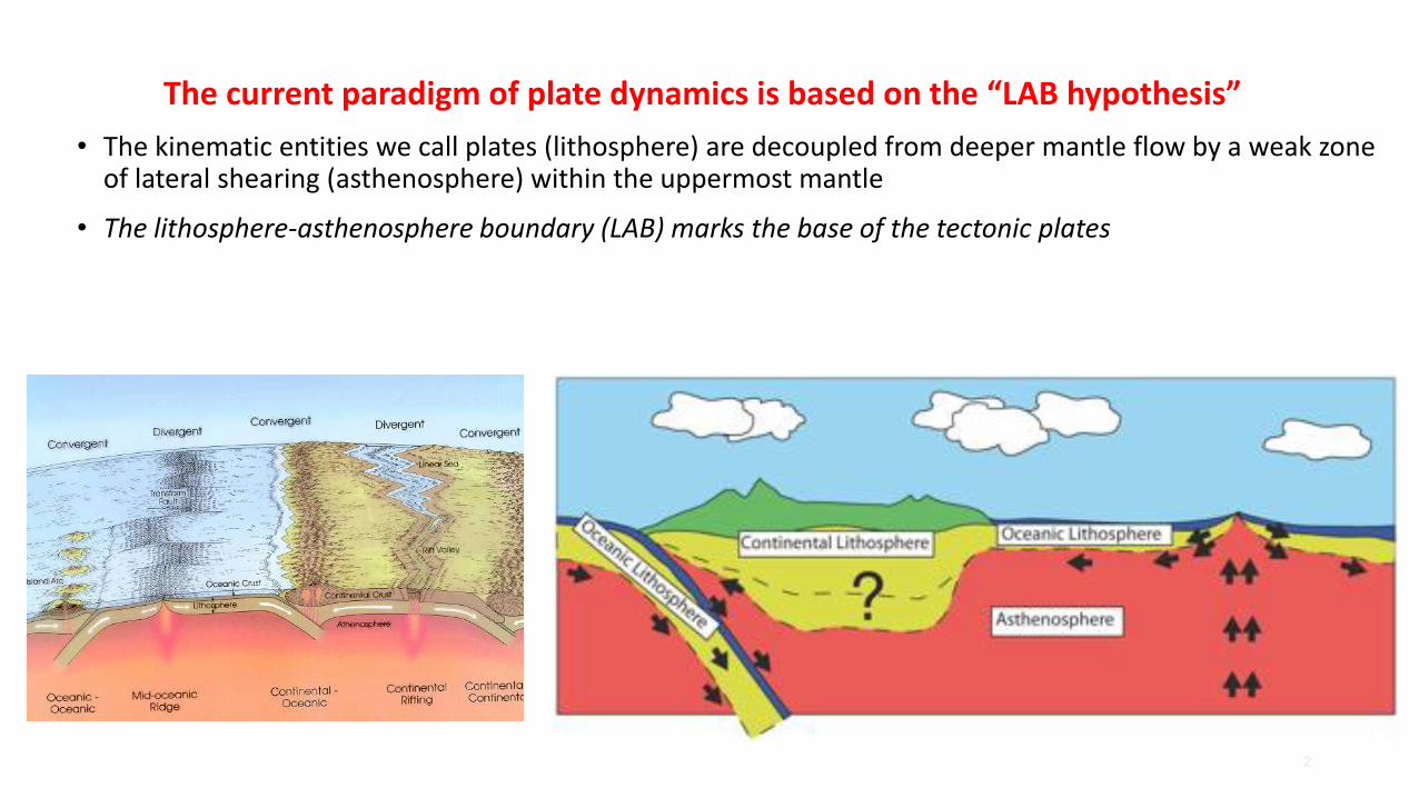
The current paradigm of plate dynamics is based on the “LAB hypothesis”

• The kinematic entities we call plates (lithosphere) are decoupled from deeper mantle flow by a weak zone of lateral shearing (asthenosphere) within the uppermost mantle

• The lithosphere-asthenosphere boundary (LAB) marks the base of the tectonic plates

2

3

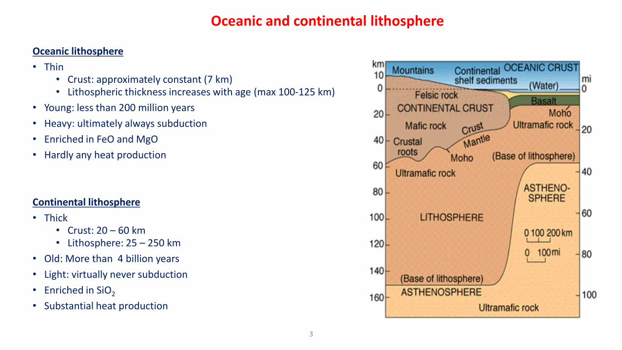
Oceanic lithosphere

• Thin• Crust: approximately constant (7 km)• Lithospheric thickness increases with age (max 100-125 km)

• Young: less than 200 million years

• Heavy: ultimately always subduction

• Enriched in FeO and MgO

• Hardly any heat production

Continental lithosphere

• Thick• Crust: 20 – 60 km• Lithosphere: 25 – 250 km

• Old: More than 4 billion years

• Light: virtually never subduction

• Enriched in SiO2

• Substantial heat production

Oceanic and continental lithosphere

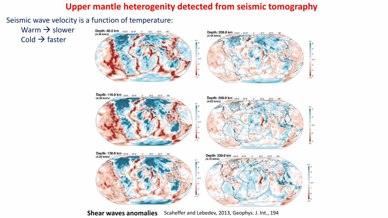
Upper mantle heterogenity detected from seismic tomography

Scaheffer and Lebedev, 2013, Geophys. J. Int., 194

Seismic wave velocity is a function of temperature:Warm slowerCold faster

Shear waves anomalies

Dependance of seismic velocities in the upper mantle

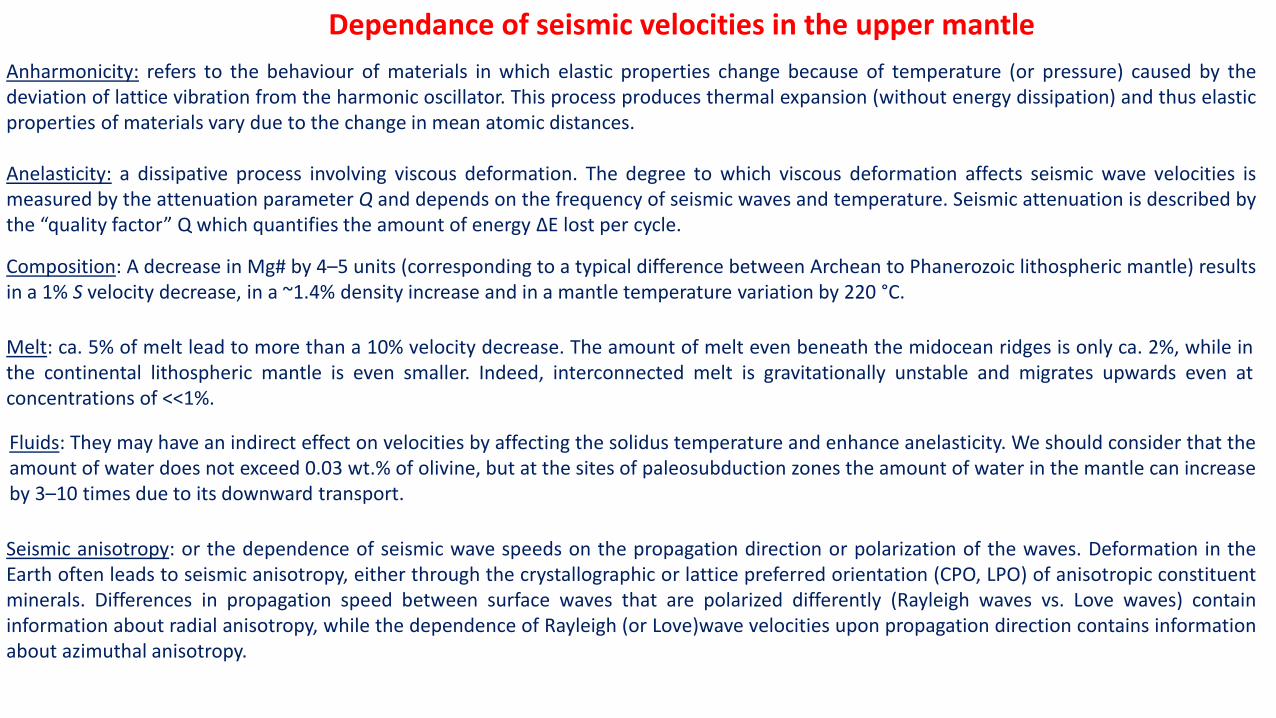
Anharmonicity: refers to the behaviour of materials in which elastic properties change because of temperature (or pressure) caused by thedeviation of lattice vibration from the harmonic oscillator. This process produces thermal expansion (without energy dissipation) and thus elasticproperties of materials vary due to the change in mean atomic distances.

Anelasticity: a dissipative process involving viscous deformation. The degree to which viscous deformation affects seismic wave velocities ismeasured by the attenuation parameter Q and depends on the frequency of seismic waves and temperature. Seismic attenuation is described bythe “quality factor” Q which quantifies the amount of energy ΔE lost per cycle.

Composition: A decrease in Mg# by 4–5 units (corresponding to a typical difference between Archean to Phanerozoic lithospheric mantle) resultsin a 1% S velocity decrease, in a ~1.4% density increase and in a mantle temperature variation by 220 °C.

Melt: ca. 5% of melt lead to more than a 10% velocity decrease. The amount of melt even beneath the midocean ridges is only ca. 2%, while inthe continental lithospheric mantle is even smaller. Indeed, interconnected melt is gravitationally unstable and migrates upwards even atconcentrations of <<1%.

Fluids: They may have an indirect effect on velocities by affecting the solidus temperature and enhance anelasticity. We should consider that theamount of water does not exceed 0.03 wt.% of olivine, but at the sites of paleosubduction zones the amount of water in the mantle can increaseby 3–10 times due to its downward transport.

Seismic anisotropy: or the dependence of seismic wave speeds on the propagation direction or polarization of the waves. Deformation in theEarth often leads to seismic anisotropy, either through the crystallographic or lattice preferred orientation (CPO, LPO) of anisotropic constituentminerals. Differences in propagation speed between surface waves that are polarized differently (Rayleigh waves vs. Love waves) containinformation about radial anisotropy, while the dependence of Rayleigh (or Love)wave velocities upon propagation direction contains informationabout azimuthal anisotropy.

Temperature (°C)

Vs (km/s)

Anel.Mod1 Anel.Mod2

Anel.Mod4

Anel.Mod3

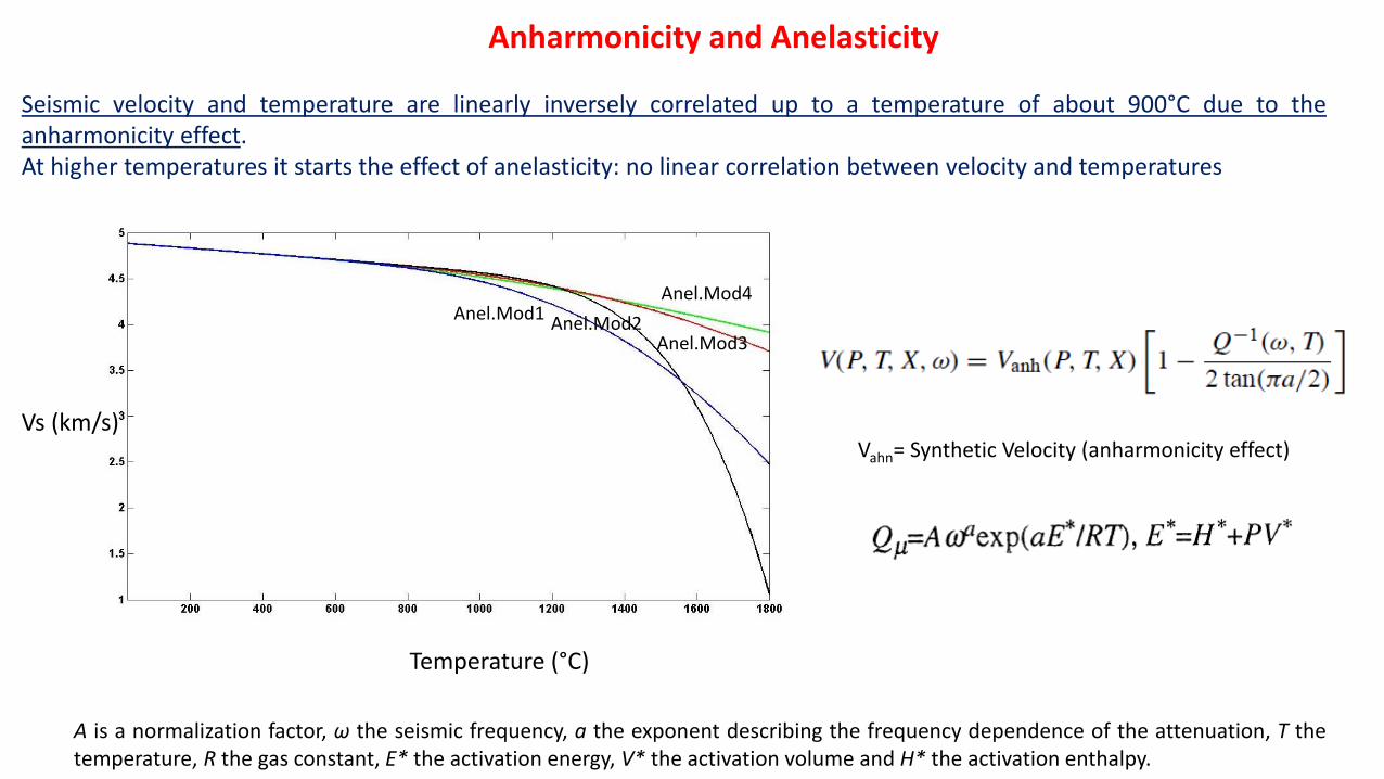
Seismic velocity and temperature are linearly inversely correlated up to a temperature of about 900°C due to theanharmonicity effect.At higher temperatures it starts the effect of anelasticity: no linear correlation between velocity and temperatures

Anharmonicity and Anelasticity

Vahn= Synthetic Velocity (anharmonicity effect)

A is a normalization factor, ω the seismic frequency, a the exponent describing the frequency dependence of the attenuation, T thetemperature, R the gas constant, E* the activation energy, V* the activation volume and H* the activation enthalpy.

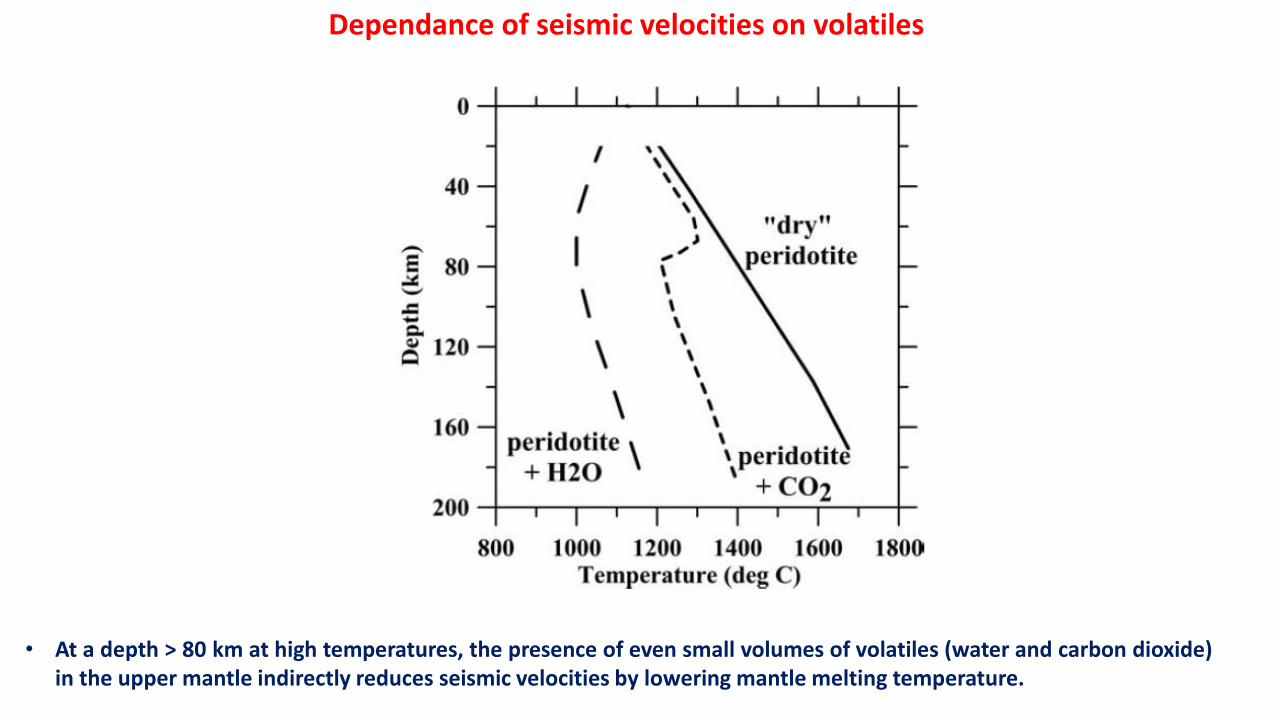
• At a depth > 80 km at high temperatures, the presence of even small volumes of volatiles (water and carbon dioxide)in the upper mantle indirectly reduces seismic velocities by lowering mantle melting temperature.

Dependance of seismic velocities on volatiles

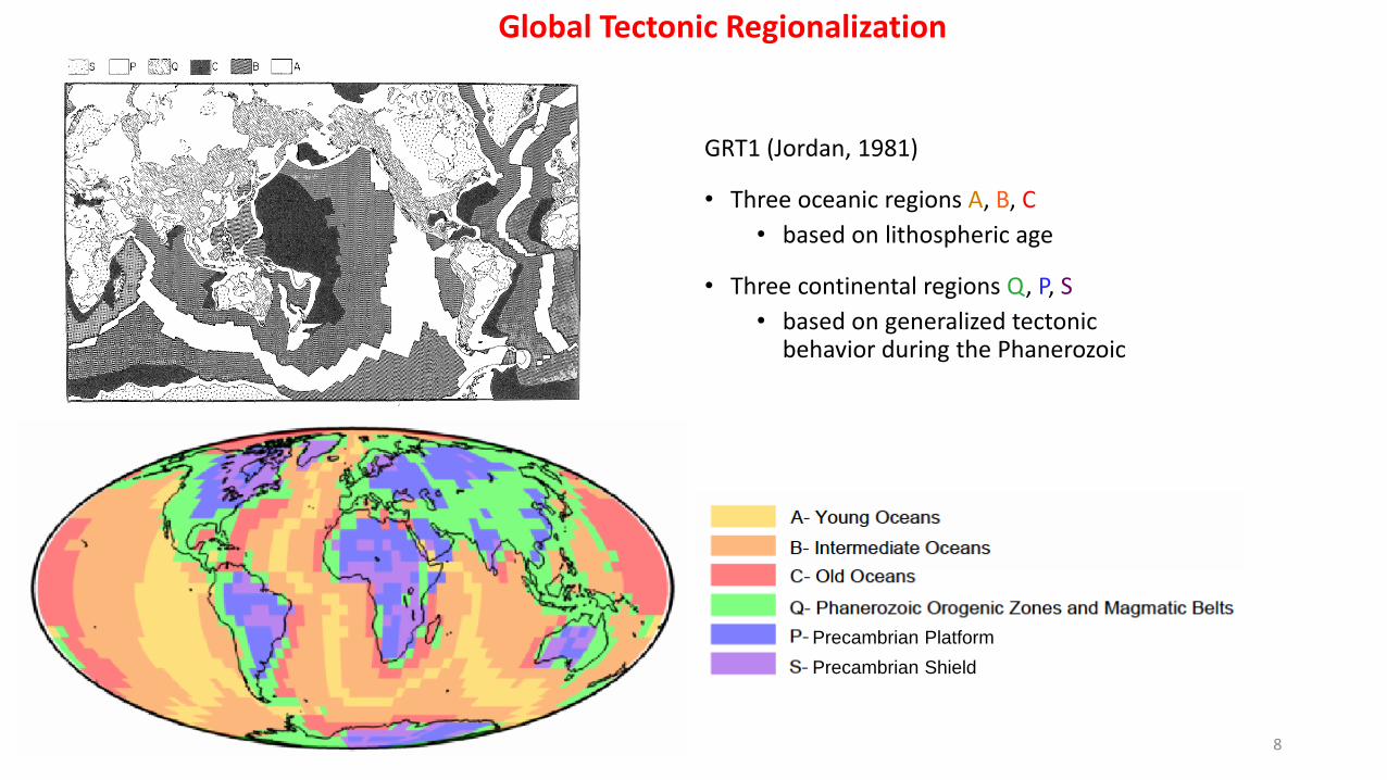
GRT1 (Jordan, 1981)

• Three oceanic regions A, B, C

• based on lithospheric age

• Three continental regions Q, P, S

• based on generalized tectonic behavior during the Phanerozoic

8

Global Tectonic Regionalization

Precambrian Shield

Precambrian Platform

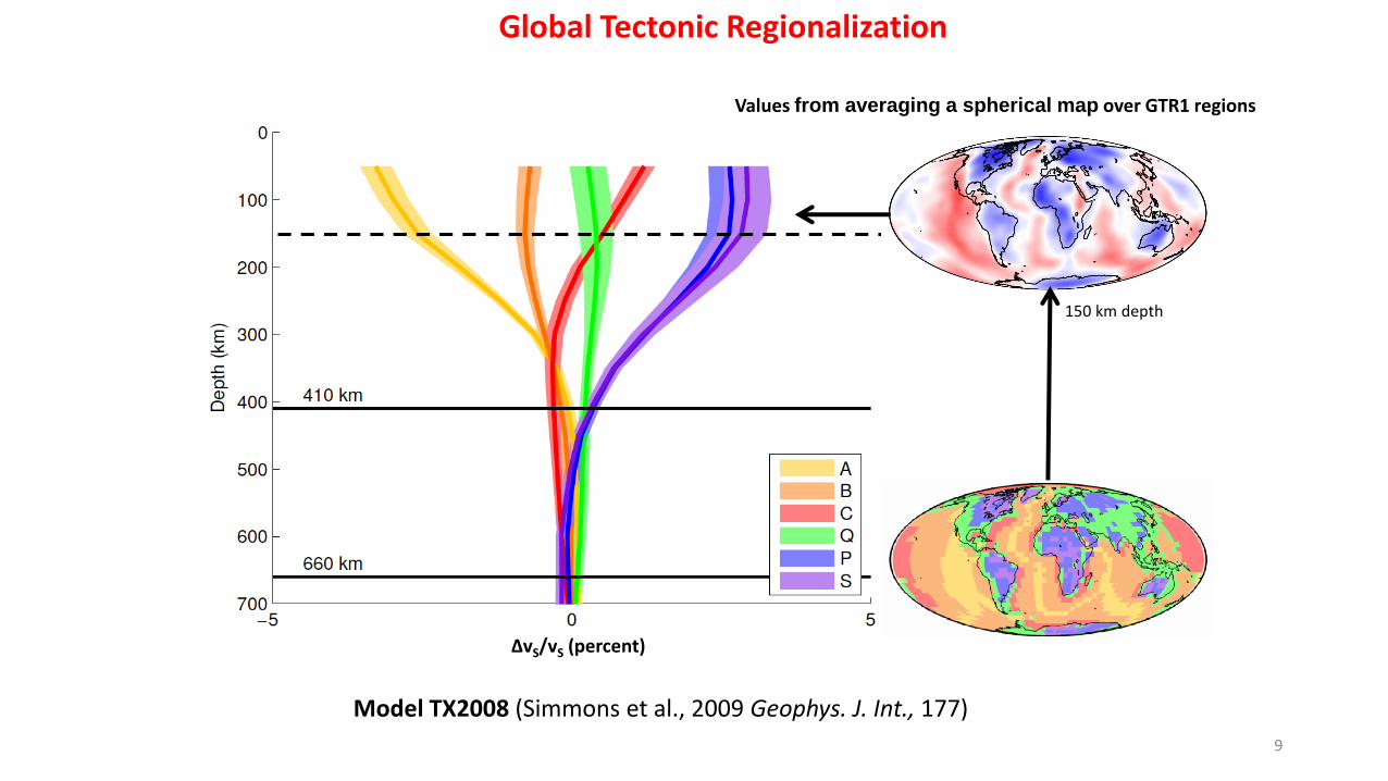
150 km depth

Model TX2008 (Simmons et al., 2009 Geophys. J. Int., 177)

ΔvS/vS (percent)

Values from averaging a spherical map over GTR1 regions

9

Global Tectonic Regionalization

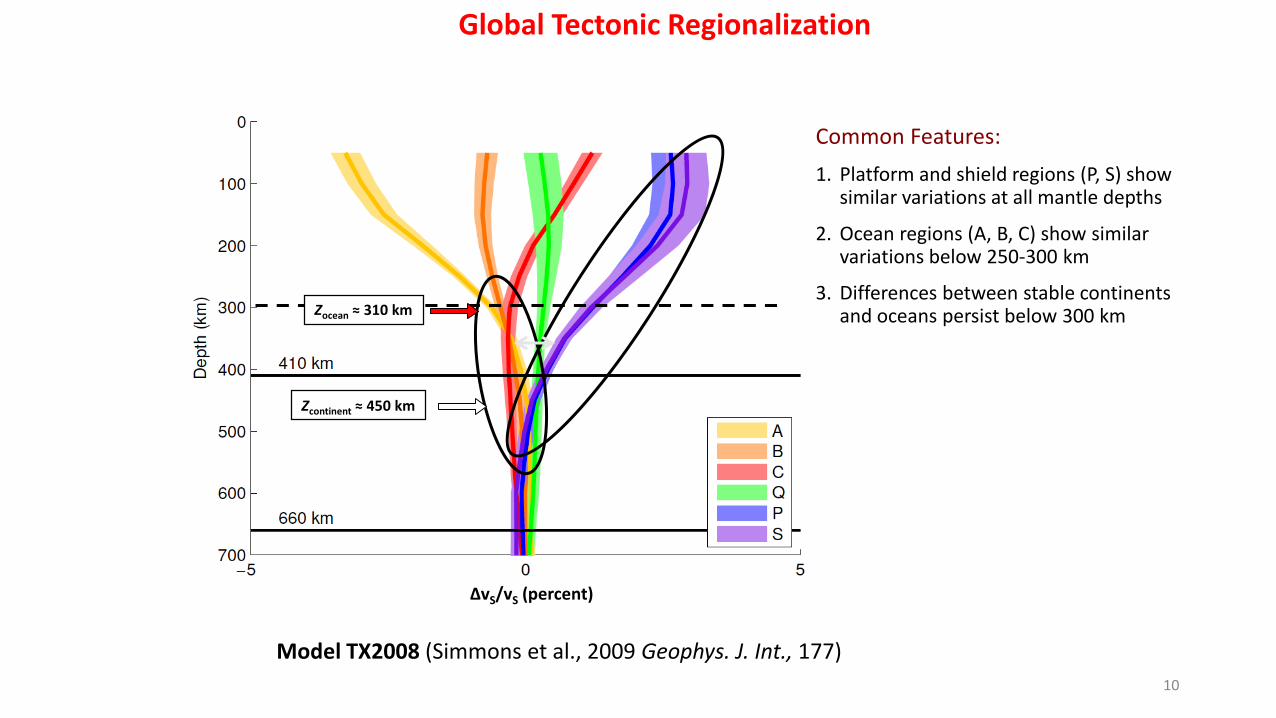
ΔvS/vS (percent)

Common Features:

1. Platform and shield regions (P, S) show similar variations at all mantle depths

2. Ocean regions (A, B, C) show similar variations below 250-300 km

3. Differences between stable continents and oceans persist below 300 km

10

Zocean ≈ 310 km

Zcontinent ≈ 450 km

Global Tectonic Regionalization

Model TX2008 (Simmons et al., 2009 Geophys. J. Int., 177)

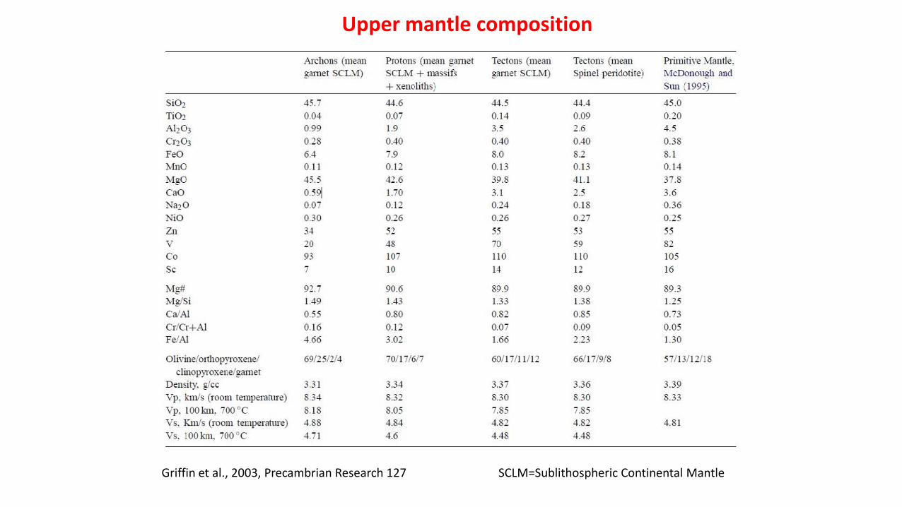
Upper mantle composition

Griffin et al., 2003, Precambrian Research 127 SCLM=Sublithospheric Continental Mantle

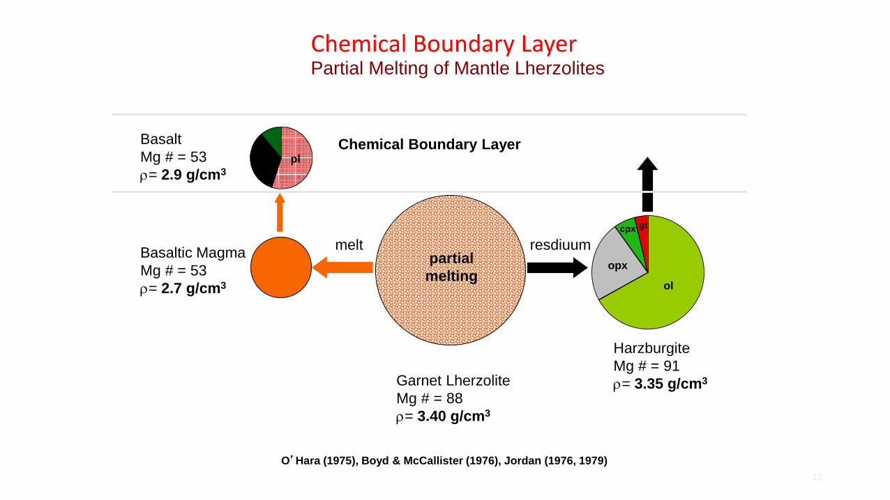
Basaltic Magma

Mg # = 53

= 2.7 g/cm3ol

opx

cpx

gt

Garnet Lherzolite

Mg # = 88

= 3.40 g/cm3

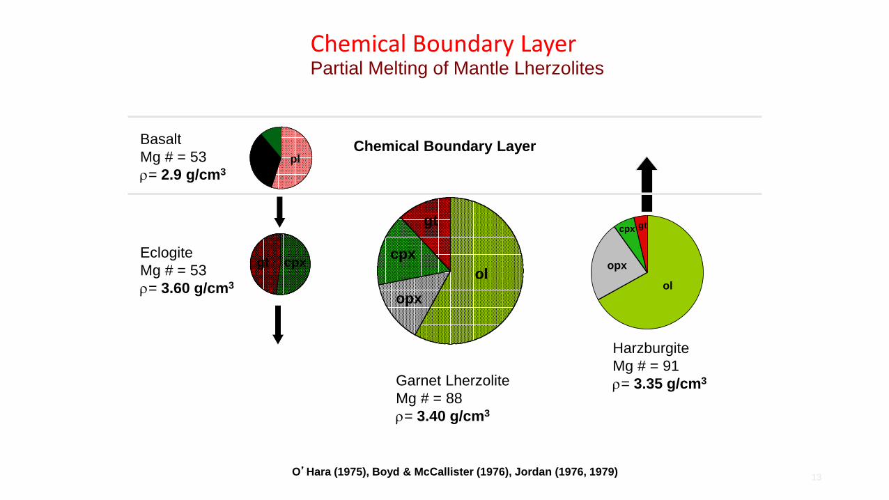
Chemical Boundary LayerPartial Melting of Mantle Lherzolites

Basalt

Mg # = 53

= 2.9 g/cm3

plcpx

ol

opx

cpx gt

Harzburgite

Mg # = 91

= 3.35 g/cm3

partial

melting

resdiuummelt

O’Hara (1975), Boyd & McCallister (1976), Jordan (1976, 1979)

12

Chemical Boundary Layer

ol

opx

cpx

gt

Garnet Lherzolite

Mg # = 88

= 3.40 g/cm3

cpxgtEclogite

Mg # = 53

= 3.60 g/cm3

Basalt

Mg # = 53

= 2.9 g/cm3

plcpx

ol

opx

cpx gt

Harzburgite

Mg # = 91

= 3.35 g/cm3

13

Chemical Boundary Layer

O’Hara (1975), Boyd & McCallister (1976), Jordan (1976, 1979)

Chemical Boundary LayerPartial Melting of Mantle Lherzolites

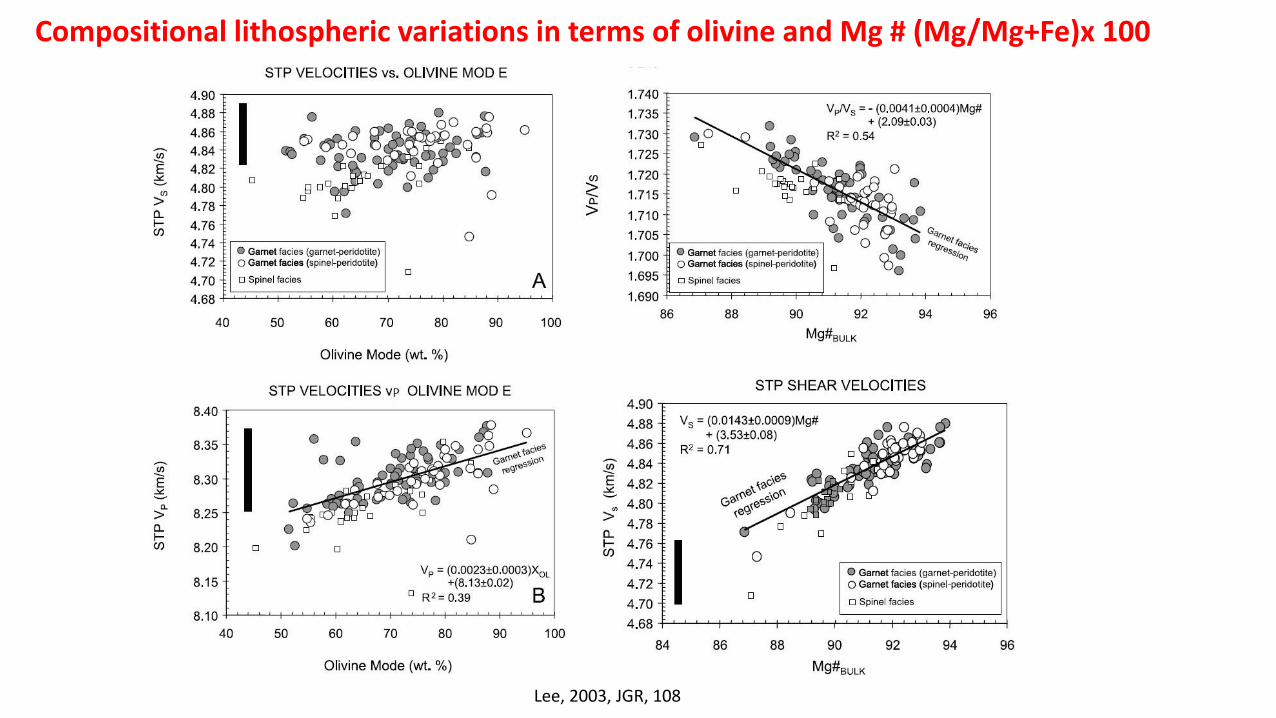
Compositional lithospheric variations in terms of olivine and Mg # (Mg/Mg+Fe)x 100

Lee, 2003, JGR, 108

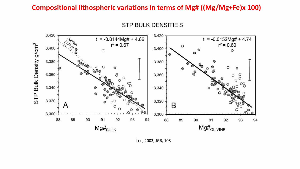
Compositional lithospheric variations in terms of Mg# ((Mg/Mg+Fe)x 100)

Lee, 2003, JGR, 108

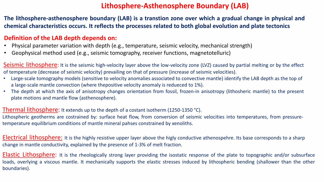
Thermal lithosphere: It extends up to the depth of a costant isotherm (1250-1350 °C).

Lithospheric geotherms are costrained by: surface heat flow, from conversion of seismic velocities into temperatures, from pressure-temperature equilibrium conditions of mantle mineral pahses constrained by xenoliths.

Seismic lithosphere: It is the seismic high-velocity layer above the low-velocity zone (LVZ) caused by partial melting or by the effect

of temperature (decrease of seismic velocity) prevailing on that of pressure (increase of seismic velocities).• Large-scale tomography models (sensitive to velocity anomalies associated to convective mantle) identify the LAB depth as the top of

a large-scale mantle convection (where thepositive velocity anomaly is redueced to 1%). • The depth at which the axis of anisotropy changes orientation from fossil, frozen-in anisotropy (lithosheric mantle) to the present

plate motions and mantle flow (asthenosphere).

Electrical lithosphere: It is the highly resistive upper layer above the higly conductive athenospehre. Its base corresponds to a sharp

change in mantle conductivity, explained by the presence of 1-3% of melt fraction.

Elastic Lithosphere: It is the rheologically strong layer providing the isostatic response of the plate to topographic and/or subsurface

loads, overlying a viscous mantle. It mechanically supports the elastic stresses induced by lithospheric bending (shallower than the otherboundaries).

The lithosphere-asthenosphere boundary (LAB) is a transtion zone over which a gradual change in physical andchemical characteristics occurs. It reflects the processes related to both global evolution and plate tectonics

Definition of the LAB depth depends on:• Physical parameter variation with depth (e.g., temperature, seismic velocity, mechanical strength)• Geophysical method used (e.g., seismic tomography, receiver functions, magnetotelluric)

Lithosphere-Asthenosphere Boundary (LAB)

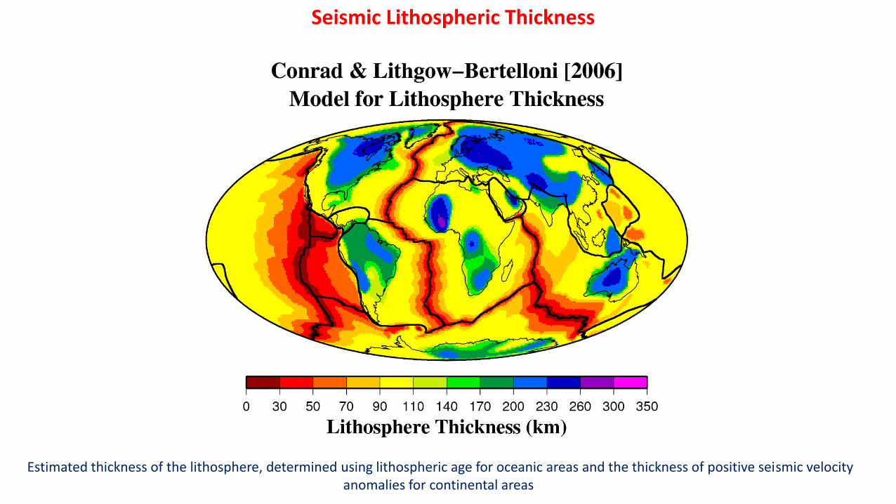
Estimated thickness of the lithosphere, determined using lithospheric age for oceanic areas and the thickness of positive seismic velocity anomalies for continental areas

Seismic Lithospheric Thickness

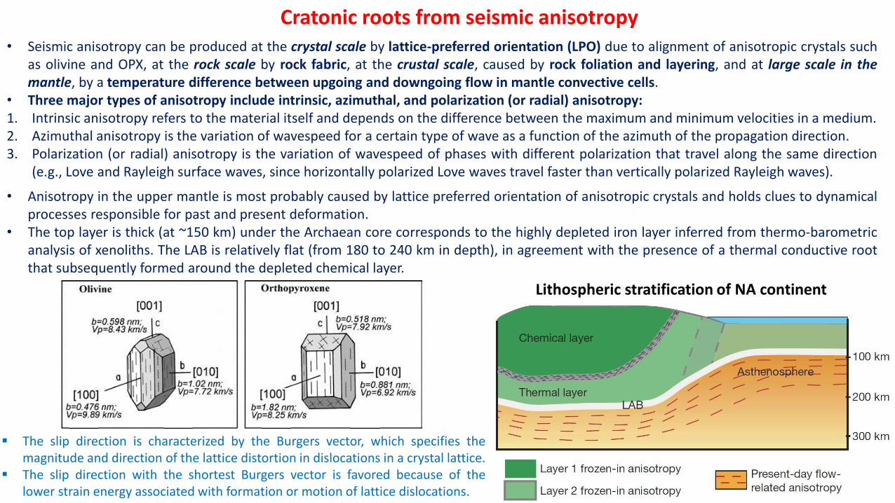
Cratonic roots from seismic anisotropy• Seismic anisotropy can be produced at the crystal scale by lattice-preferred orientation (LPO) due to alignment of anisotropic crystals such

as olivine and OPX, at the rock scale by rock fabric, at the crustal scale, caused by rock foliation and layering, and at large scale in themantle, by a temperature difference between upgoing and downgoing flow in mantle convective cells.

• Three major types of anisotropy include intrinsic, azimuthal, and polarization (or radial) anisotropy:1. Intrinsic anisotropy refers to the material itself and depends on the difference between the maximum and minimum velocities in a medium.2. Azimuthal anisotropy is the variation of wavespeed for a certain type of wave as a function of the azimuth of the propagation direction.3. Polarization (or radial) anisotropy is the variation of wavespeed of phases with different polarization that travel along the same direction

(e.g., Love and Rayleigh surface waves, since horizontally polarized Love waves travel faster than vertically polarized Rayleigh waves).

• Anisotropy in the upper mantle is most probably caused by lattice preferred orientation of anisotropic crystals and holds clues to dynamicalprocesses responsible for past and present deformation.

• The top layer is thick (at ~150 km) under the Archaean core corresponds to the highly depleted iron layer inferred from thermo-barometricanalysis of xenoliths. The LAB is relatively flat (from 180 to 240 km in depth), in agreement with the presence of a thermal conductive rootthat subsequently formed around the depleted chemical layer.

The slip direction is characterized by the Burgers vector, which specifies themagnitude and direction of the lattice distortion in dislocations in a crystal lattice.

The slip direction with the shortest Burgers vector is favored because of thelower strain energy associated with formation or motion of lattice dislocations.

Lithospheric stratification of NA continent

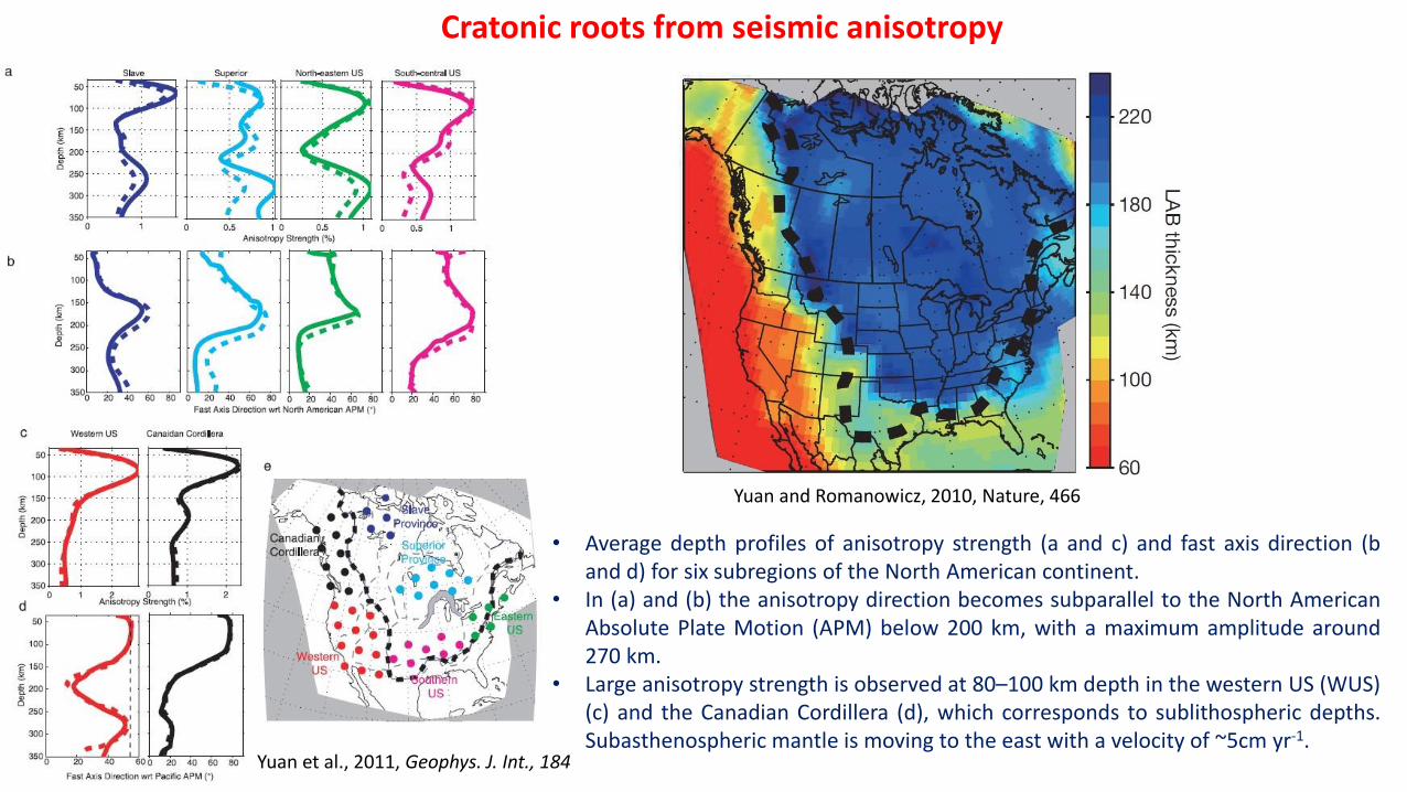
Yuan and Romanowicz, 2010, Nature, 466

Yuan et al., 2011, Geophys. J. Int., 184

Cratonic roots from seismic anisotropy

• Average depth profiles of anisotropy strength (a and c) and fast axis direction (band d) for six subregions of the North American continent.

• In (a) and (b) the anisotropy direction becomes subparallel to the North AmericanAbsolute Plate Motion (APM) below 200 km, with a maximum amplitude around270 km.

• Large anisotropy strength is observed at 80–100 km depth in the western US (WUS)(c) and the Canadian Cordillera (d), which corresponds to sublithospheric depths.Subasthenospheric mantle is moving to the east with a velocity of ~5cm yr-1.

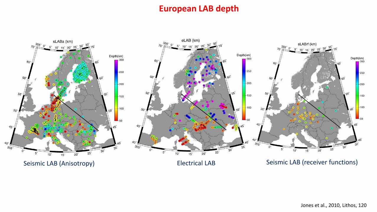
European LAB depth

Seismic LAB (Anisotropy) Seismic LAB (receiver functions)Electrical LAB

Jones et al., 2010, Lithos, 120

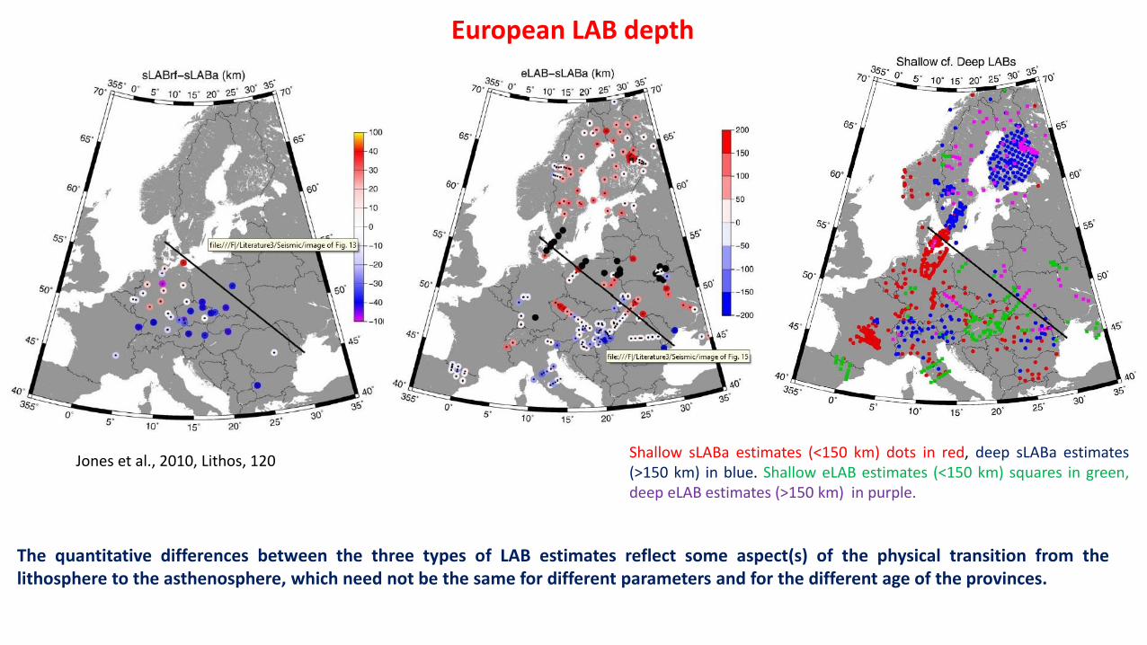
European LAB depth

Jones et al., 2010, Lithos, 120Shallow sLABa estimates (<150 km) dots in red, deep sLABa estimates(>150 km) in blue. Shallow eLAB estimates (<150 km) squares in green,deep eLAB estimates (>150 km) in purple.

The quantitative differences between the three types of LAB estimates reflect some aspect(s) of the physical transition from thelithosphere to the asthenosphere, which need not be the same for different parameters and for the different age of the provinces.

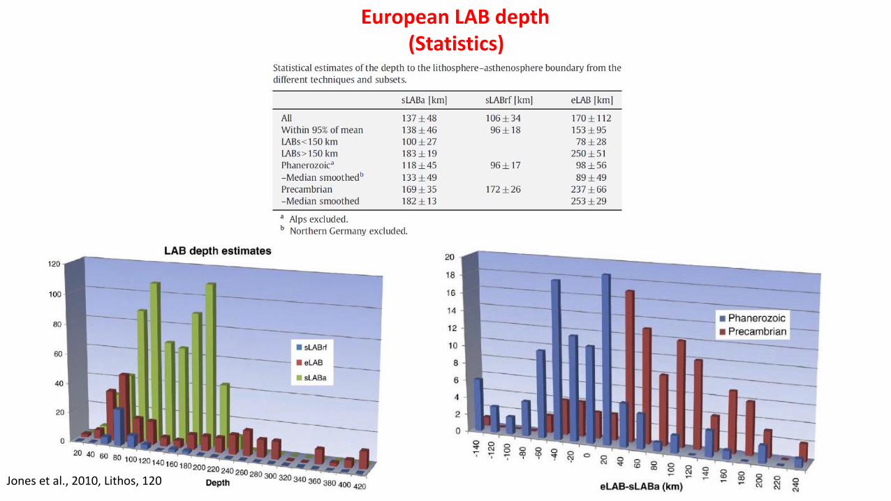
Jones et al., 2010, Lithos, 120

European LAB depth(Statistics)

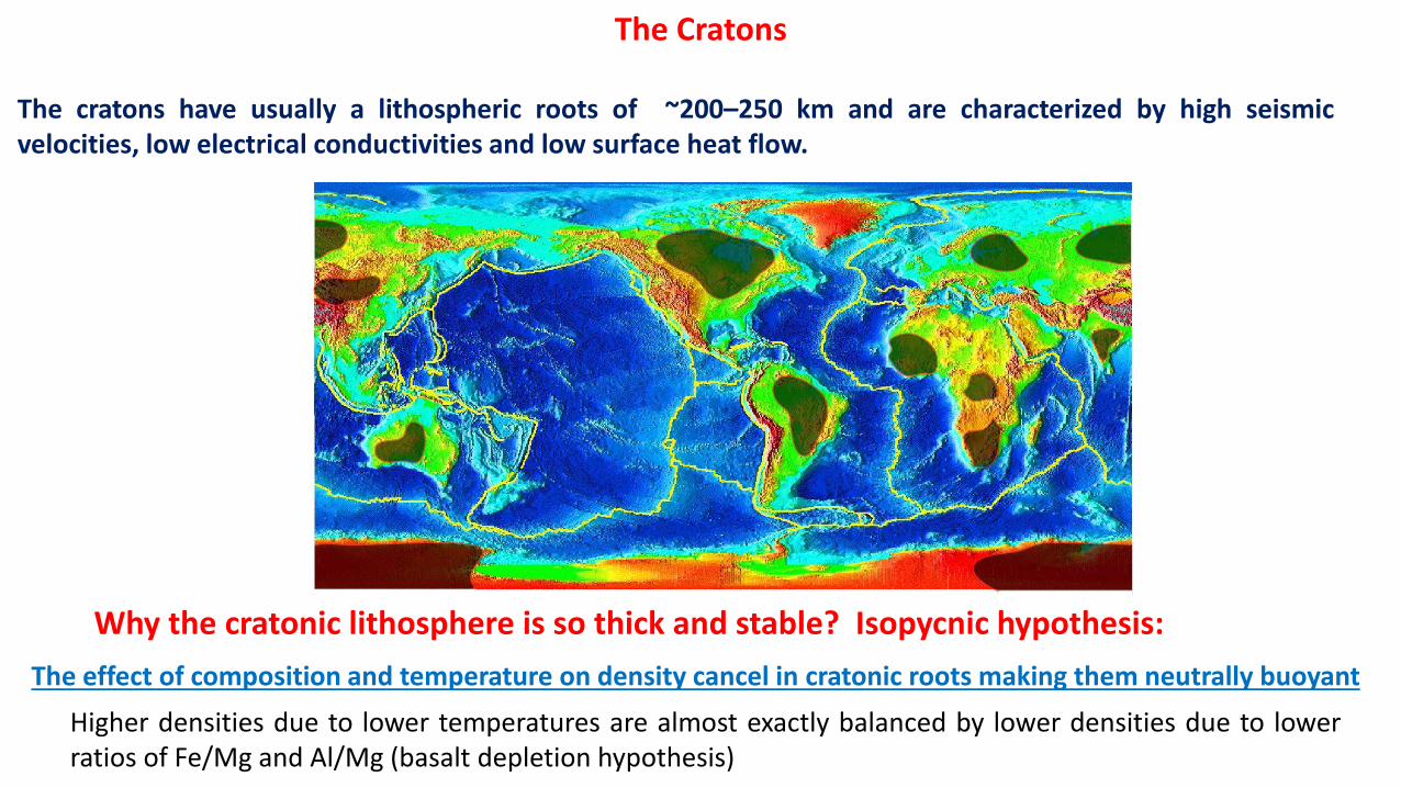
Why the cratonic lithosphere is so thick and stable? Isopycnic hypothesis:

The effect of composition and temperature on density cancel in cratonic roots making them neutrally buoyant

Higher densities due to lower temperatures are almost exactly balanced by lower densities due to lowerratios of Fe/Mg and Al/Mg (basalt depletion hypothesis)

The cratons have usually a lithospheric roots of ~200–250 km and are characterized by high seismicvelocities, low electrical conductivities and low surface heat flow.

The Cratons

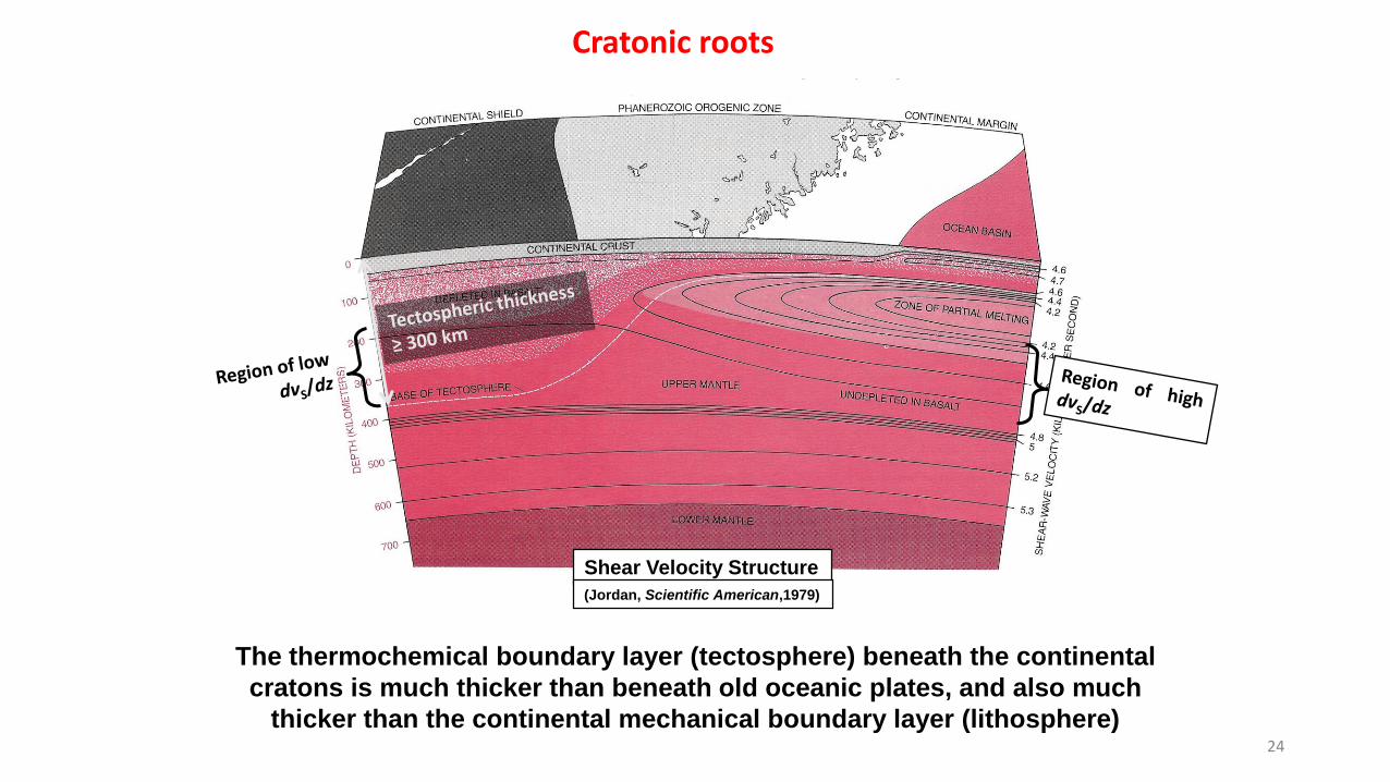
Shear Velocity Structure

Cratonic roots

The thermochemical boundary layer (tectosphere) beneath the continental

cratons is much thicker than beneath old oceanic plates, and also much

thicker than the continental mechanical boundary layer (lithosphere)

(Jordan, Scientific American,1979)

24

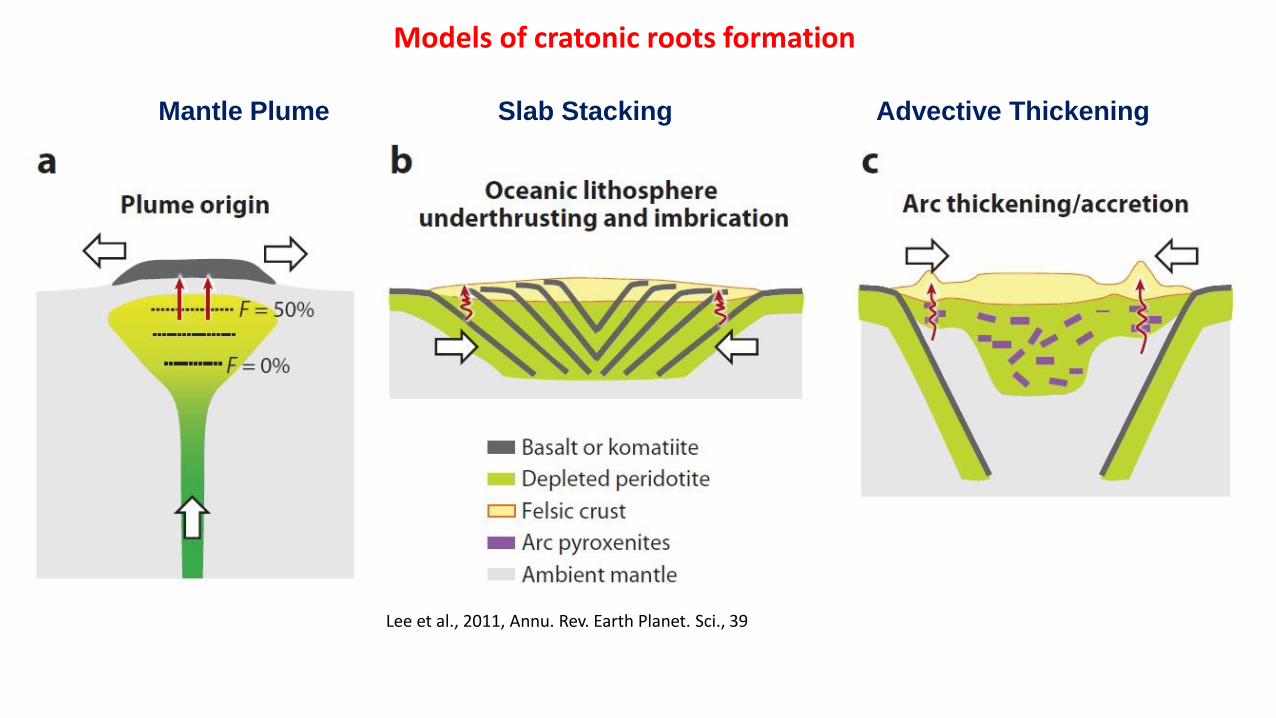
Models of cratonic roots formation

Mantle Plume Slab Stacking Advective Thickening

Lee et al., 2011, Annu. Rev. Earth Planet. Sci., 39

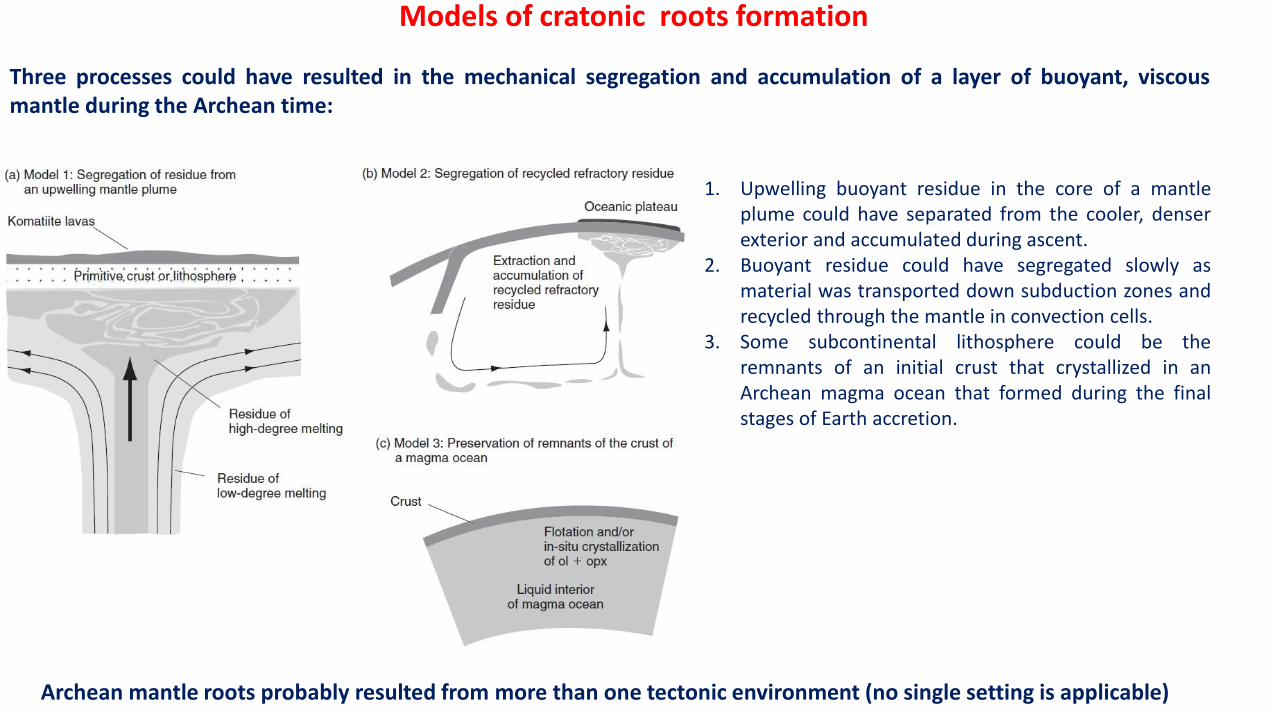
Models of cratonic roots formation

Three processes could have resulted in the mechanical segregation and accumulation of a layer of buoyant, viscousmantle during the Archean time:

1. Upwelling buoyant residue in the core of a mantleplume could have separated from the cooler, denserexterior and accumulated during ascent.

2. Buoyant residue could have segregated slowly asmaterial was transported down subduction zones andrecycled through the mantle in convection cells.

3. Some subcontinental lithosphere could be theremnants of an initial crust that crystallized in anArchean magma ocean that formed during the finalstages of Earth accretion.

Archean mantle roots probably resulted from more than one tectonic environment (no single setting is applicable)

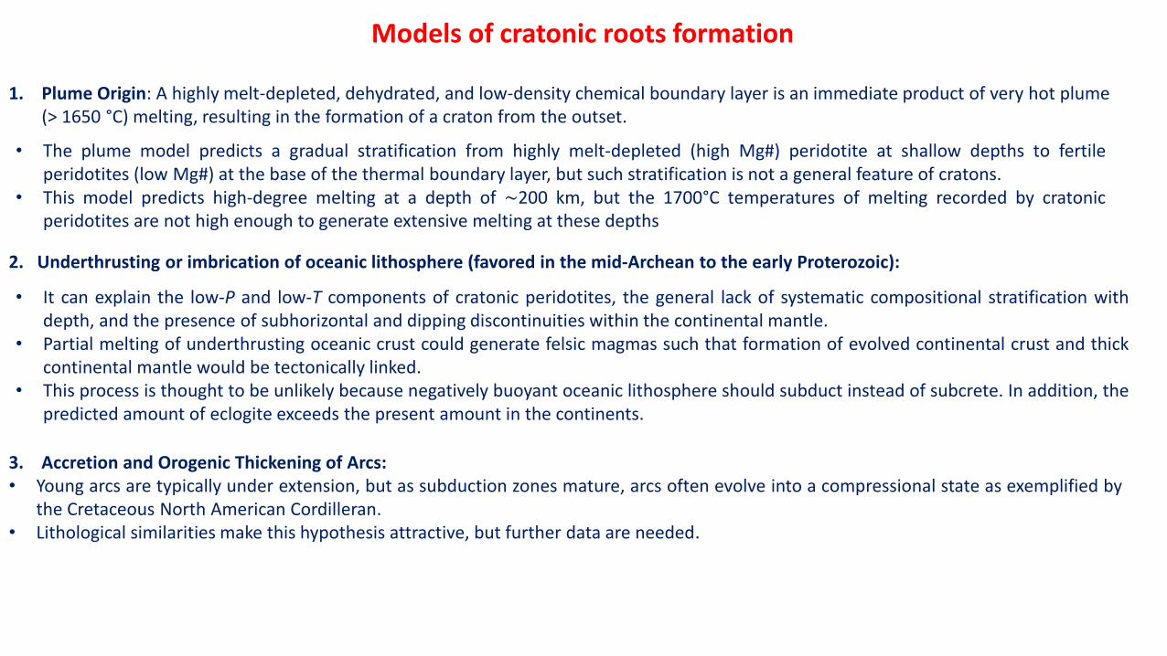
• The plume model predicts a gradual stratification from highly melt-depleted (high Mg#) peridotite at shallow depths to fertileperidotites (low Mg#) at the base of the thermal boundary layer, but such stratification is not a general feature of cratons.

• This model predicts high-degree melting at a depth of ∼200 km, but the 1700°C temperatures of melting recorded by cratonicperidotites are not high enough to generate extensive melting at these depths

1. Plume Origin: A highly melt-depleted, dehydrated, and low-density chemical boundary layer is an immediate product of very hot plume (> 1650 °C) melting, resulting in the formation of a craton from the outset.

• It can explain the low-P and low-T components of cratonic peridotites, the general lack of systematic compositional stratification withdepth, and the presence of subhorizontal and dipping discontinuities within the continental mantle.

• Partial melting of underthrusting oceanic crust could generate felsic magmas such that formation of evolved continental crust and thickcontinental mantle would be tectonically linked.

• This process is thought to be unlikely because negatively buoyant oceanic lithosphere should subduct instead of subcrete. In addition, thepredicted amount of eclogite exceeds the present amount in the continents.

2. Underthrusting or imbrication of oceanic lithosphere (favored in the mid-Archean to the early Proterozoic):

Models of cratonic roots formation

3. Accretion and Orogenic Thickening of Arcs:• Young arcs are typically under extension, but as subduction zones mature, arcs often evolve into a compressional state as exemplified by

the Cretaceous North American Cordilleran.• Lithological similarities make this hypothesis attractive, but further data are needed.

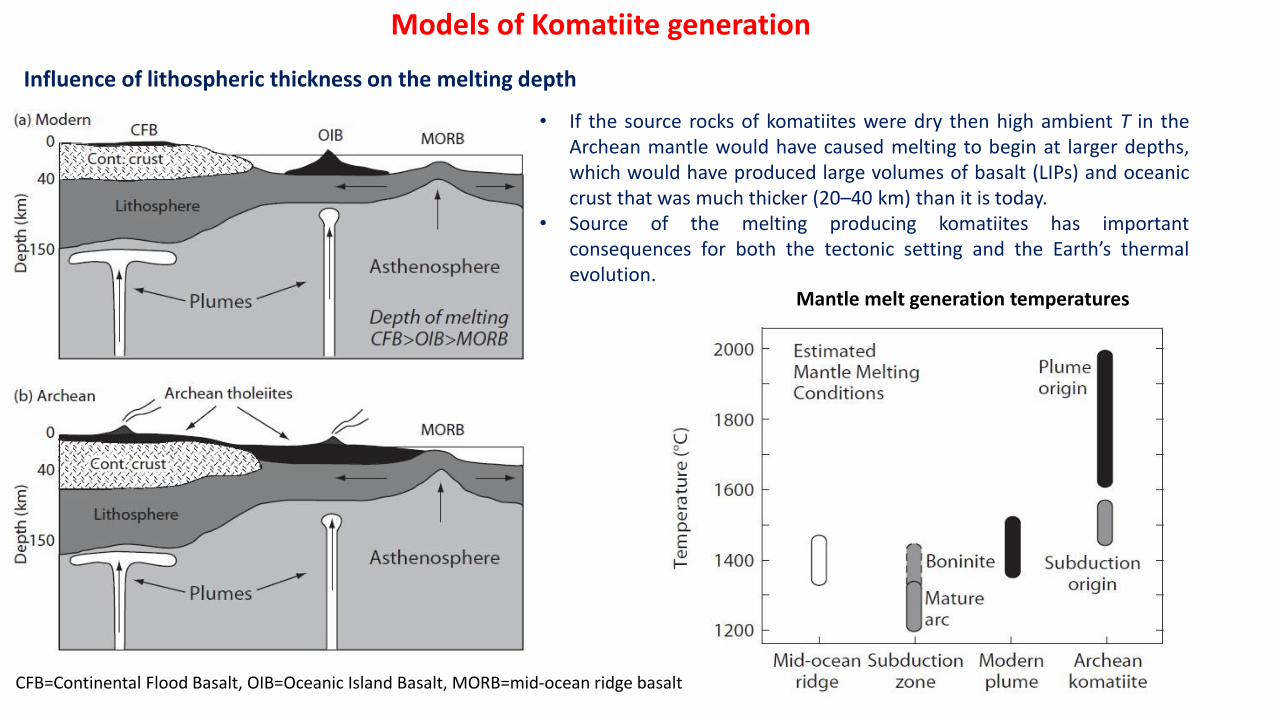
Models of Komatiite generation

• If the source rocks of komatiites were dry then high ambient T in theArchean mantle would have caused melting to begin at larger depths,which would have produced large volumes of basalt (LIPs) and oceaniccrust that was much thicker (20–40 km) than it is today.

• Source of the melting producing komatiites has importantconsequences for both the tectonic setting and the Earth’s thermalevolution.

Influence of lithospheric thickness on the melting depth

CFB=Continental Flood Basalt, OIB=Oceanic Island Basalt, MORB=mid-ocean ridge basalt

Mantle melt generation temperatures

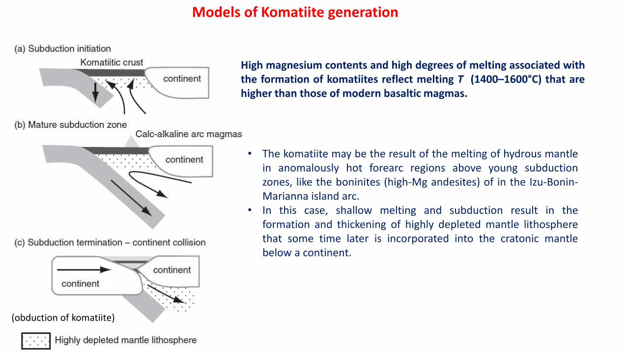
Models of Komatiite generation

High magnesium contents and high degrees of melting associated withthe formation of komatiites reflect melting T (1400–1600°C) that arehigher than those of modern basaltic magmas.

• The komatiite may be the result of the melting of hydrous mantlein anomalously hot forearc regions above young subductionzones, like the boninites (high-Mg andesites) of in the Izu-Bonin-Marianna island arc.

• In this case, shallow melting and subduction result in theformation and thickening of highly depleted mantle lithospherethat some time later is incorporated into the cratonic mantlebelow a continent.

(obduction of komatiite)

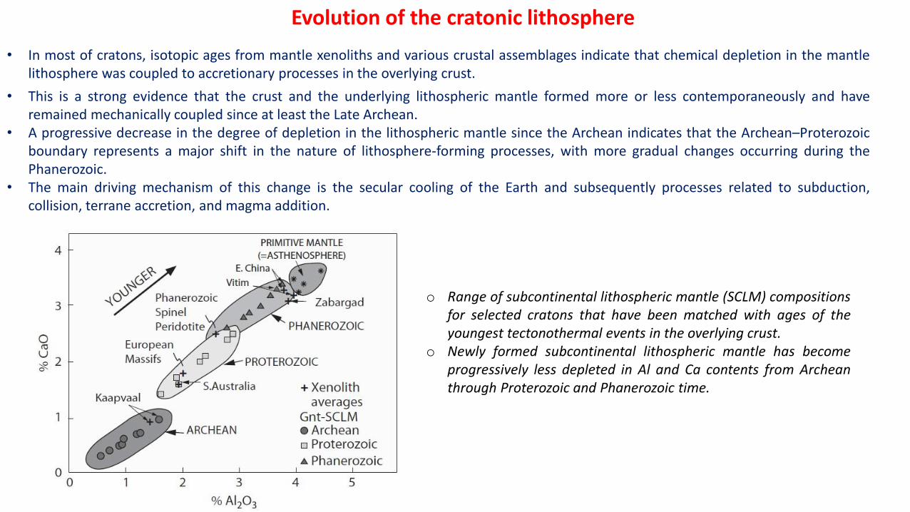
Evolution of the cratonic lithosphere

• In most of cratons, isotopic ages from mantle xenoliths and various crustal assemblages indicate that chemical depletion in the mantlelithosphere was coupled to accretionary processes in the overlying crust.

• This is a strong evidence that the crust and the underlying lithospheric mantle formed more or less contemporaneously and haveremained mechanically coupled since at least the Late Archean.

• A progressive decrease in the degree of depletion in the lithospheric mantle since the Archean indicates that the Archean–Proterozoicboundary represents a major shift in the nature of lithosphere-forming processes, with more gradual changes occurring during thePhanerozoic.

• The main driving mechanism of this change is the secular cooling of the Earth and subsequently processes related to subduction,collision, terrane accretion, and magma addition.

o Range of subcontinental lithospheric mantle (SCLM) compositionsfor selected cratons that have been matched with ages of theyoungest tectonothermal events in the overlying crust.

o Newly formed subcontinental lithospheric mantle has becomeprogressively less depleted in Al and Ca contents from Archeanthrough Proterozoic and Phanerozoic time.

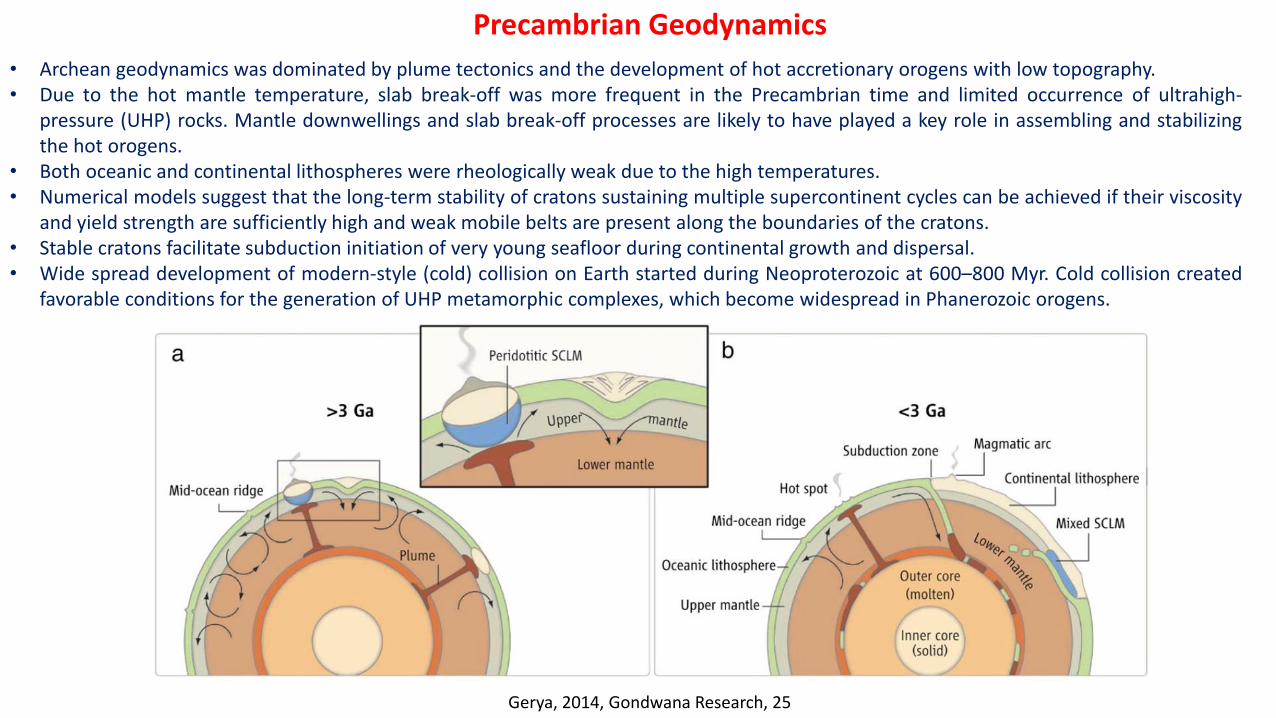
• Archean geodynamics was dominated by plume tectonics and the development of hot accretionary orogens with low topography.• Due to the hot mantle temperature, slab break-off was more frequent in the Precambrian time and limited occurrence of ultrahigh-

pressure (UHP) rocks. Mantle downwellings and slab break-off processes are likely to have played a key role in assembling and stabilizingthe hot orogens.

• Both oceanic and continental lithospheres were rheologically weak due to the high temperatures.• Numerical models suggest that the long-term stability of cratons sustaining multiple supercontinent cycles can be achieved if their viscosity

and yield strength are sufficiently high and weak mobile belts are present along the boundaries of the cratons.• Stable cratons facilitate subduction initiation of very young seafloor during continental growth and dispersal.• Wide spread development of modern-style (cold) collision on Earth started during Neoproterozoic at 600–800 Myr. Cold collision created

favorable conditions for the generation of UHP metamorphic complexes, which become widespread in Phanerozoic orogens.

Precambrian Geodynamics

Gerya, 2014, Gondwana Research, 25

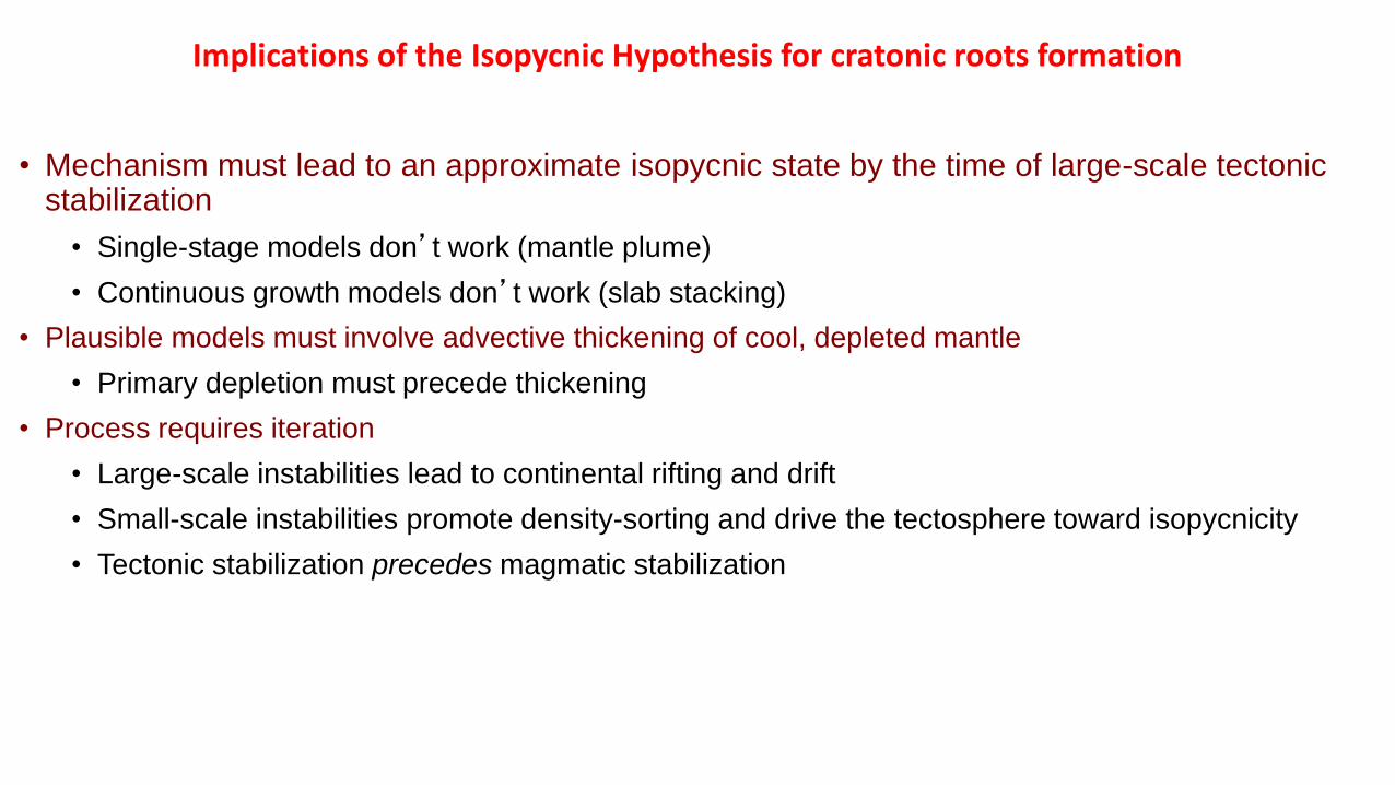
• Mechanism must lead to an approximate isopycnic state by the time of large-scale tectonic stabilization

• Single-stage models don’t work (mantle plume)

• Continuous growth models don’t work (slab stacking)

• Plausible models must involve advective thickening of cool, depleted mantle

• Primary depletion must precede thickening

• Process requires iteration

• Large-scale instabilities lead to continental rifting and drift

• Small-scale instabilities promote density-sorting and drive the tectosphere toward isopycnicity

• Tectonic stabilization precedes magmatic stabilization

Implications of the Isopycnic Hypothesis for cratonic roots formation

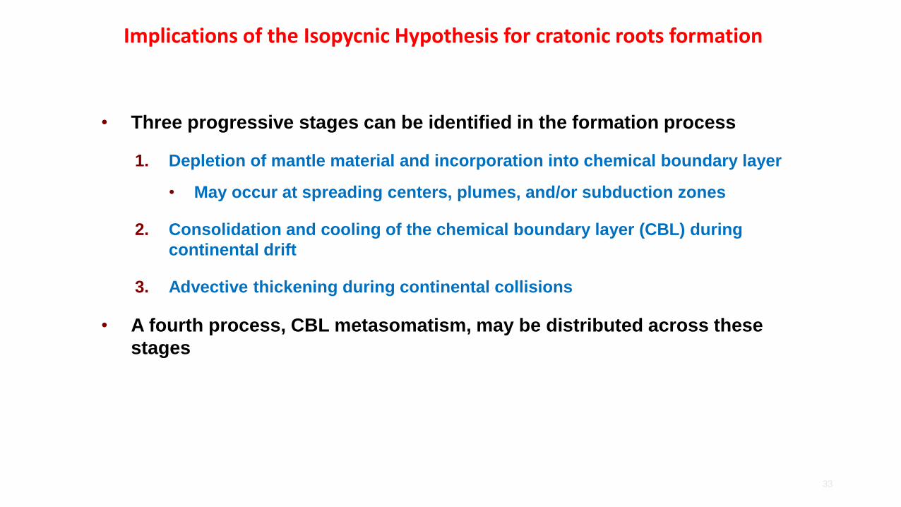
• Three progressive stages can be identified in the formation process

1. Depletion of mantle material and incorporation into chemical boundary layer

• May occur at spreading centers, plumes, and/or subduction zones

2. Consolidation and cooling of the chemical boundary layer (CBL) during

continental drift

3. Advective thickening during continental collisions

• A fourth process, CBL metasomatism, may be distributed across these

stages

33

Implications of the Isopycnic Hypothesis for cratonic roots formation

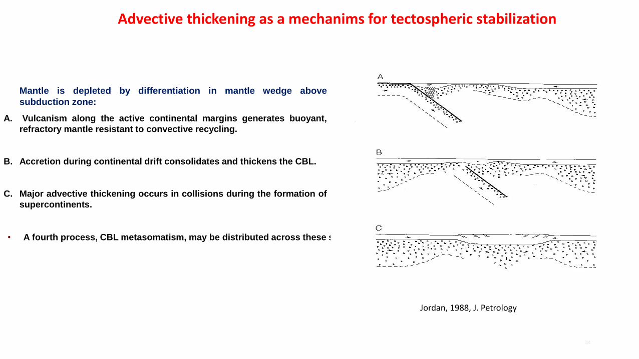
Jordan, 1988, J. Petrology

A. Mantle is depleted by differentiation in mantle wedge above

subduction zone:

A. Vulcanism along the active continental margins generates buoyant,

refractory mantle resistant to convective recycling.

B. Accretion during continental drift consolidates and thickens the CBL.

C. Major advective thickening occurs in collisions during the formation of

supercontinents.

34

Advective thickening as a mechanims for tectospheric stabilization

• A fourth process, CBL metasomatism, may be distributed across these stages

Crustal Structure of South African Craton

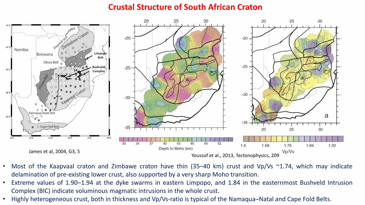
• Most of the Kaapvaal craton and Zimbawe craton have thin (35–40 km) crust and Vp/Vs ~1.74, which may indicatedelamination of pre-existing lower crust, also supported by a very sharp Moho transition.

• Extreme values of 1.90–1.94 at the dyke swarms in eastern Limpopo, and 1.84 in the easternmost Bushveld IntrusionComplex (BIC) indicate voluminous magmatic intrusions in the whole crust.

• Highly heterogeneous crust, both in thickness and Vp/Vs-ratio is typical of the Namaqua–Natal and Cape Fold Belts.

Youssof et al., 2013, Tectonophysics, 209James et al, 2004, G3, 5

approximate thickness of

lithosphere?

Kaapvaal cratonBushveld

Old

ocean

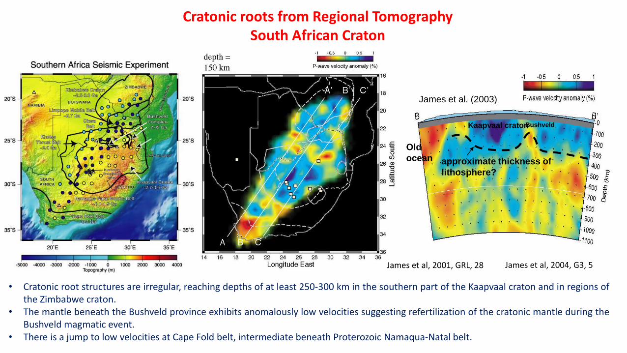
James et al. (2003)

Cratonic roots from Regional TomographySouth African Craton

• Cratonic root structures are irregular, reaching depths of at least 250-300 km in the southern part of the Kaapvaal craton and in regions ofthe Zimbabwe craton.

• The mantle beneath the Bushveld province exhibits anomalously low velocities suggesting refertilization of the cratonic mantle during theBushveld magmatic event.

• There is a jump to low velocities at Cape Fold belt, intermediate beneath Proterozoic Namaqua-Natal belt.

James et al, 2004, G3, 5James et al, 2001, GRL, 28

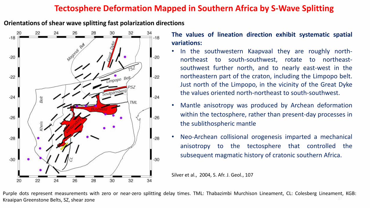
Tectosphere Deformation Mapped in Southern Africa by S-Wave Splitting

The values of lineation direction exhibit systematic spatialvariations:• In the southwestern Kaapvaal they are roughly north-

northeast to south-southwest, rotate to northeast-southwest further north, and to nearly east-west in thenortheastern part of the craton, including the Limpopo belt.Just north of the Limpopo, in the vicinity of the Great Dykethe values oriented north-northeast to south-southwest.

• Mantle anisotropy was produced by Archean deformation

within the tectosphere, rather than present-day processes in

the sublithospheric mantle

• Neo-Archean collisional orogenesis imparted a mechanical

anisotropy to the tectosphere that controlled the

subsequent magmatic history of cratonic southern Africa.

Silver et al., 2004, S. Afr. J. Geol., 107

37

Orientations of shear wave splitting fast polarization directions

Purple dots represent measurements with zero or near-zero splitting delay times. TML: Thabazimbi Murchison Lineament, CL: Colesberg Lineament, KGB:Kraaipan Greenstone Belts, SZ, shear zone

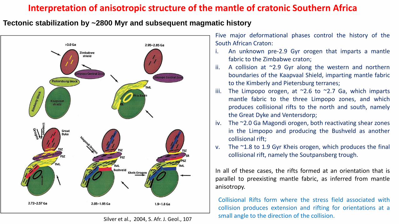
Interpretation of anisotropic structure of the mantle of cratonic Southern Africa

Five major deformational phases control the history of theSouth African Craton:i. An unknown pre-2.9 Gyr orogen that imparts a mantle

fabric to the Zimbabwe craton;ii. A collision at ~2.9 Gyr along the western and northern

boundaries of the Kaapvaal Shield, imparting mantle fabricto the Kimberly and Pietersburg terranes;

iii. The Limpopo orogen, at ~2.6 to ~2.7 Ga, which impartsmantle fabric to the three Limpopo zones, and whichproduces collisional rifts to the north and south, namelythe Great Dyke and Ventersdorp;

iv. The ~2.0 Ga Magondi orogen, both reactivating shear zonesin the Limpopo and producing the Bushveld as anothercollisional rift;

v. The ~1.8 to 1.9 Gyr Kheis orogen, which produces the finalcollisional rift, namely the Soutpansberg trough.

In all of these cases, the rifts formed at an orientation that isparallel to preexisting mantle fabric, as inferred from mantleanisotropy.

Collisional Rifts form where the stress field associated withcollision produces extension and rifting for orientations at asmall angle to the direction of the collision.

Tectonic stabilization by ~2800 Myr and subsequent magmatic history

Silver et al., 2004, S. Afr. J. Geol., 107

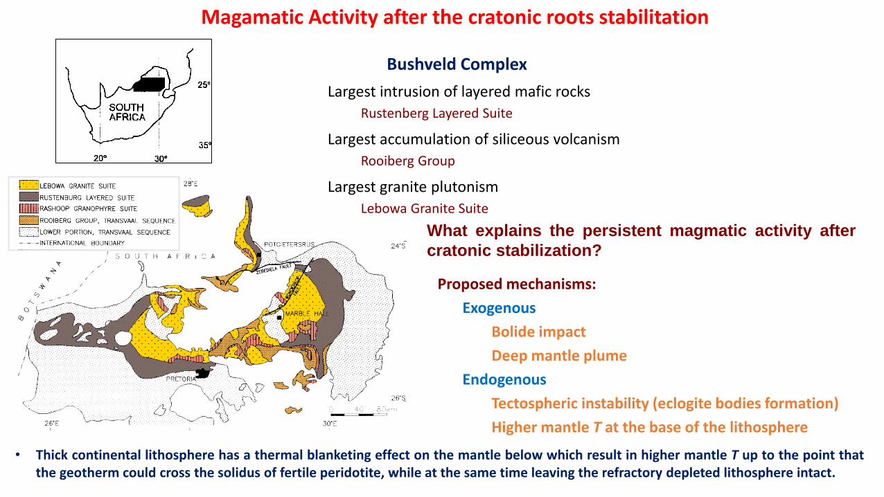
Proposed mechanisms:

l Exogenous

Bolide impact

Deep mantle plume

l Endogenous

Tectospheric instability (eclogite bodies formation)

Higher mantle T at the base of the lithosphere

39

What explains the persistent magmatic activity after

cratonic stabilization?

• Largest intrusion of layered mafic rocks

• Rustenberg Layered Suite

• Largest accumulation of siliceous volcanism

• Rooiberg Group

• Largest granite plutonism

• Lebowa Granite Suite

• Thick continental lithosphere has a thermal blanketing effect on the mantle below which result in higher mantle T up to the point thatthe geotherm could cross the solidus of fertile peridotite, while at the same time leaving the refractory depleted lithosphere intact.

Magamatic Activity after the cratonic roots stabilitation

Bushveld Complex

Chemical Limitations on Cratonic Growth

Observations:

• Isopycnicity implies thick tectosphere stabilized by depleted peridotites

• Highly depleted, low-density peridotites (Mg # > 92) observed in the subcratonic mantle areprimarily of Archean age

• Subsequent Proterozoic and Phanerozoic magmatism has not generated large volumes of suchrocks

Implication:

• Proterozoic transition from thick to relatively thin tectosphere can plausibly be explained by theexhaustion of Archean mantle peridotitites with Mg # > 92

Why do older continental cratons have thicker tectosphere than younger continents?

40

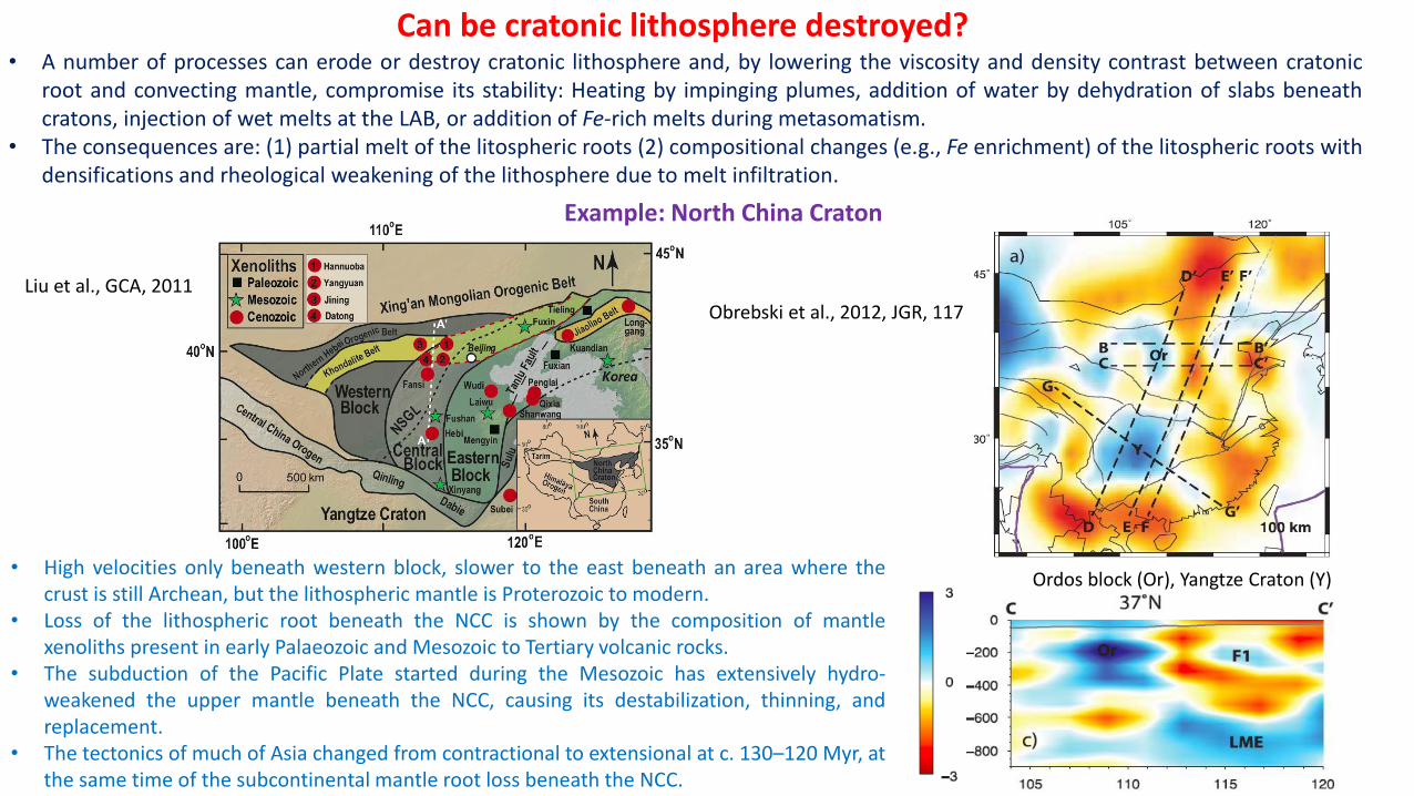
• A number of processes can erode or destroy cratonic lithosphere and, by lowering the viscosity and density contrast between cratonicroot and convecting mantle, compromise its stability: Heating by impinging plumes, addition of water by dehydration of slabs beneathcratons, injection of wet melts at the LAB, or addition of Fe-rich melts during metasomatism.

• The consequences are: (1) partial melt of the litospheric roots (2) compositional changes (e.g., Fe enrichment) of the litospheric roots withdensifications and rheological weakening of the lithosphere due to melt infiltration.

Can be cratonic lithosphere destroyed?

Ordos block (Or), Yangtze Craton (Y)• High velocities only beneath western block, slower to the east beneath an area where the

crust is still Archean, but the lithospheric mantle is Proterozoic to modern.• Loss of the lithospheric root beneath the NCC is shown by the composition of mantle

xenoliths present in early Palaeozoic and Mesozoic to Tertiary volcanic rocks.• The subduction of the Pacific Plate started during the Mesozoic has extensively hydro-

weakened the upper mantle beneath the NCC, causing its destabilization, thinning, andreplacement.

• The tectonics of much of Asia changed from contractional to extensional at c. 130–120 Myr, atthe same time of the subcontinental mantle root loss beneath the NCC.

Example: North China Craton

Obrebski et al., 2012, JGR, 117

Liu et al., GCA, 2011

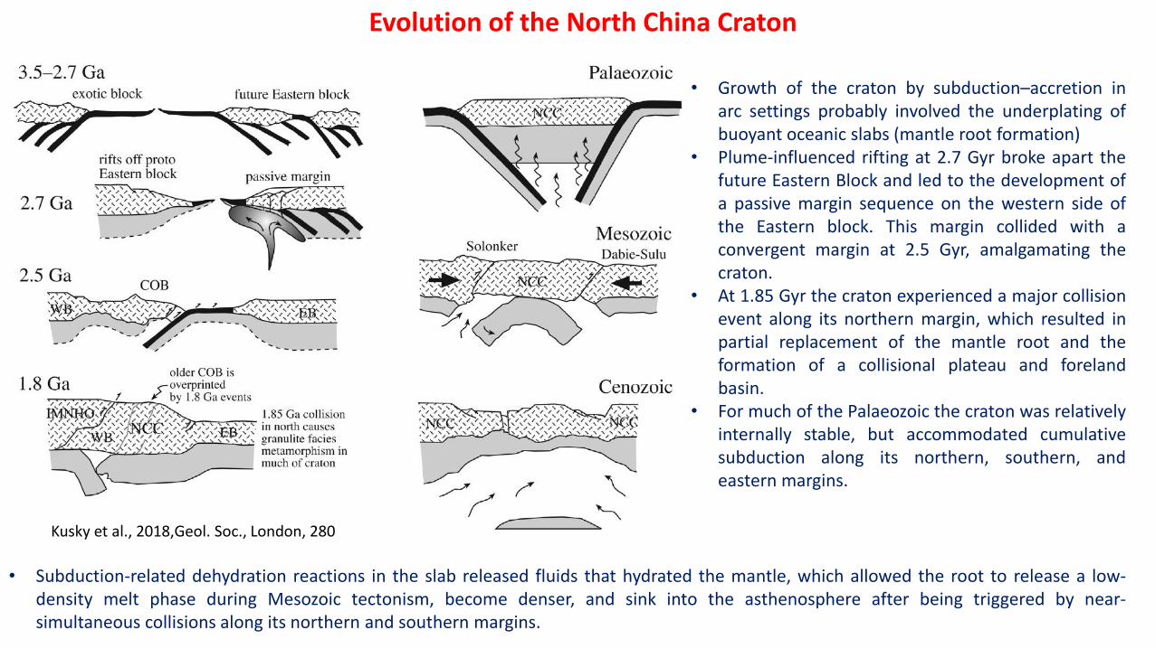
Evolution of the North China Craton

• Growth of the craton by subduction–accretion inarc settings probably involved the underplating ofbuoyant oceanic slabs (mantle root formation)

• Plume-influenced rifting at 2.7 Gyr broke apart thefuture Eastern Block and led to the development ofa passive margin sequence on the western side ofthe Eastern block. This margin collided with aconvergent margin at 2.5 Gyr, amalgamating thecraton.

• At 1.85 Gyr the craton experienced a major collisionevent along its northern margin, which resulted inpartial replacement of the mantle root and theformation of a collisional plateau and forelandbasin.

• For much of the Palaeozoic the craton was relativelyinternally stable, but accommodated cumulativesubduction along its northern, southern, andeastern margins.

• Subduction-related dehydration reactions in the slab released fluids that hydrated the mantle, which allowed the root to release a low-density melt phase during Mesozoic tectonism, become denser, and sink into the asthenosphere after being triggered by near-simultaneous collisions along its northern and southern margins.

Kusky et al., 2018,Geol. Soc., London, 280

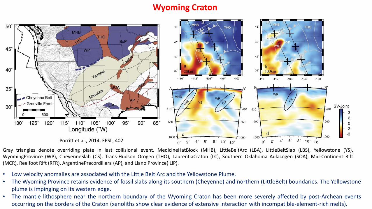
Wyoming Craton

Gray triangles denote overriding plate in last collisional event. MedicineHatBlock (MHB), LittleBeltArc (LBA), LittleBeltSlab (LBS), Yellowstone (YS),WyomingProvince (WP), CheyenneSlab (CS), Trans-Hudson Orogen (THO), LaurentiaCraton (LC), Southern Oklahoma Aulacogen (SOA), Mid-Continent Rift(MCR), Reelfoot Rift (RFR), ArgentinePrecordillera (AP), and Llano Province( LlP).

• Low velocity anomalies are associated with the Little Belt Arc and the Yellowstone Plume.• The Wyoming Province retains evidence of fossil slabs along its southern (Cheyenne) and northern (LittleBelt) boundaries. The Yellowstone

plume is impinging on its western edge.• The mantle lithosphere near the northern boundary of the Wyoming Craton has been more severely affected by post-Archean events

occurring on the borders of the Craton (xenoliths show clear evidence of extensive interaction with incompatible-element-rich melts).

Porritt et al., 2014, EPSL, 402

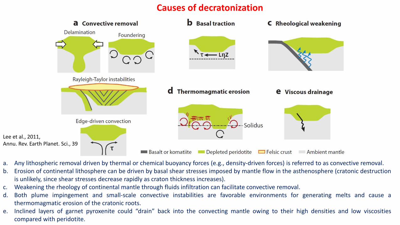
Causes of decratonization

a. Any lithospheric removal driven by thermal or chemical buoyancy forces (e.g., density-driven forces) is referred to as convective removal.b. Erosion of continental lithosphere can be driven by basal shear stresses imposed by mantle flow in the asthenosphere (cratonic destruction

is unlikely, since shear stresses decrease rapidly as craton thickness increases).c. Weakening the rheology of continental mantle through fluids infiltration can facilitate convective removal.d. Both plume impingement and small-scale convective instabilities are favorable environments for generating melts and cause a

thermomagmatic erosion of the cratonic roots.e. Inclined layers of garnet pyroxenite could “drain” back into the convecting mantle owing to their high densities and low viscosities

compared with peridotite.

Lee et al., 2011,Annu. Rev. Earth Planet. Sci., 39

Middle Lithosphere Discontinuity (MLD)

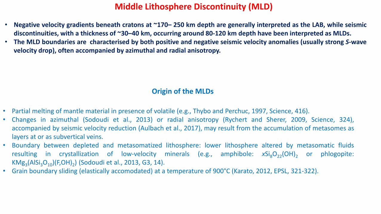
• Partial melting of mantle material in presence of volatile (e.g., Thybo and Perchuc, 1997, Science, 416).• Changes in azimuthal (Sodoudi et al., 2013) or radial anisotropy (Rychert and Sherer, 2009, Science, 324),

accompanied by seismic velocity reduction (Aulbach et al., 2017), may result from the accumulation of metasomes aslayers at or as subvertical veins.

• Boundary between depleted and metasomatized lithosphere: lower lithosphere altered by metasomatic fluidsresulting in crystallization of low-velocity minerals (e.g., amphibole: xSi8O22(OH)2 or phlogopite:KMg3(AlSi3O10)(F,OH)2) (Sodoudi et al., 2013, G3, 14).

• Grain boundary sliding (elastically accomodated) at a temperature of 900°C (Karato, 2012, EPSL, 321-322).

• Negative velocity gradients beneath cratons at ~170– 250 km depth are generally interpreted as the LAB, while seismicdiscontinuities, with a thickness of ~30–40 km, occurring around 80-120 km depth have been interpreted as MLDs.

• The MLD boundaries are characterised by both positive and negative seismic velocity anomalies (usually strong S-wavevelocity drop), often accompanied by azimuthal and radial anisotropy.

Origin of the MLDs

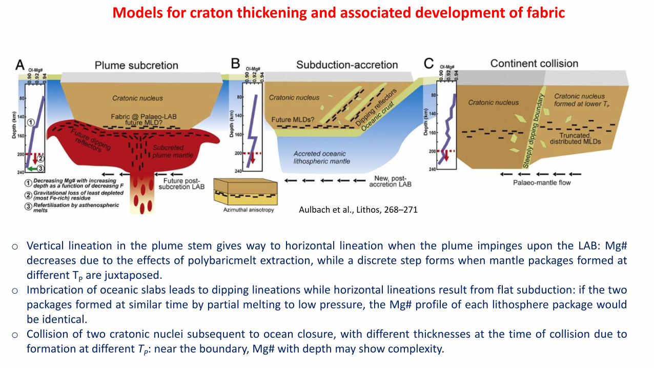
Models for craton thickening and associated development of fabric

o Vertical lineation in the plume stem gives way to horizontal lineation when the plume impinges upon the LAB: Mg#decreases due to the effects of polybaricmelt extraction, while a discrete step forms when mantle packages formed atdifferent TP are juxtaposed.

o Imbrication of oceanic slabs leads to dipping lineations while horizontal lineations result from flat subduction: if the twopackages formed at similar time by partial melting to low pressure, the Mg# profile of each lithosphere package wouldbe identical.

o Collision of two cratonic nuclei subsequent to ocean closure, with different thicknesses at the time of collision due toformation at different TP: near the boundary, Mg# with depth may show complexity.

Aulbach et al., Lithos, 268–271

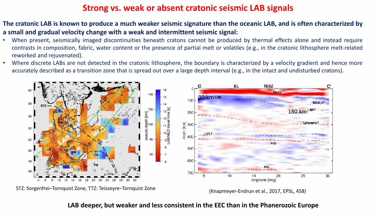
LAB deeper, but weaker and less consistent in the EEC than in the Phanerozoic Europe

(Knapmeyer-Endrun et al., 2017, EPSL, 458)

90 km

180 km

The cratonic LAB is known to produce a much weaker seismic signature than the oceanic LAB, and is often characterized bya small and gradual velocity change with a weak and intermittent seismic signal:• When present, seismically imaged discontinuities beneath cratons cannot be produced by thermal effects alone and instead require

contrasts in composition, fabric, water content or the presence of partial melt or volatiles (e.g., in the cratonic lithosphere melt-relatedreworked and rejuvenated).

• Where discrete LABs are not detected in the cratonic lithosphere, the boundary is characterized by a velocity gradient and hence moreaccurately described as a transition zone that is spread out over a large depth interval (e.g., in the intact and undisturbed cratons).

Strong vs. weak or absent cratonic seismic LAB signals

STZ: Sorgenfrei–Tornquist Zone, TTZ: Teisseyre–Tornquist Zone

• Knowledge of the present thermal state of the Earth is crucial for models of crustal and mantle evolution, mantle dynamics,and processes of deep interior.

Thermal state of the lithosphere(why do we want to know it?)

• Physical properties of crustal and mantle rocks are temperature dependant (density, seismic velocity, seismic attenuation, electrical conductivity, viscosity).

Temperature of the Earth is controlled by internal heat:

80% from the radiogenic heat production and 20 % comes from secular cooling of the Earth.

Heat is transferred to the surface of the Earth through three mechanisms: conduction (in the lithosphere), convection(below the lithosphere), and advection (hydrothermal circluation in sediments).

Knowledge of the thermal state of the lithosphere from more than 20000 heat flux measurements at the Earth’s surface

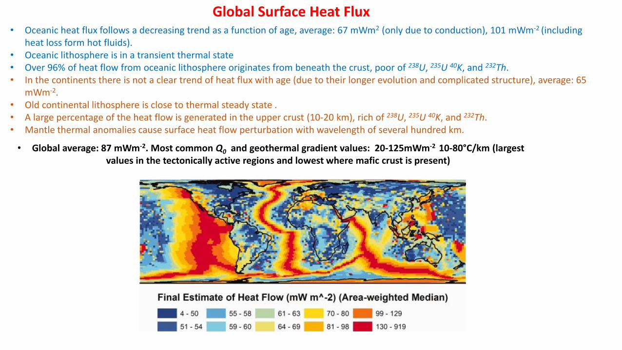
Global Surface Heat Flux• Oceanic heat flux follows a decreasing trend as a function of age, average: 67 mWm2 (only due to conduction), 101 mWm-2 (including

heat loss form hot fluids).• Oceanic lithosphere is in a transient thermal state • Over 96% of heat flow from oceanic lithosphere originates from beneath the crust, poor of 238U, 235U 40K, and 232Th.• In the continents there is not a clear trend of heat flux with age (due to their longer evolution and complicated structure), average: 65

mWm-2. • Old continental lithosphere is close to thermal steady state .• A large percentage of the heat flow is generated in the upper crust (10-20 km), rich of 238U, 235U 40K, and 232Th.• Mantle thermal anomalies cause surface heat flow perturbation with wavelength of several hundred km.

• Global average: 87 mWm-2. Most common Q0 and geothermal gradient values: 20-125mWm-2 10-80°C/km (largest values in the tectonically active regions and lowest where mafic crust is present)

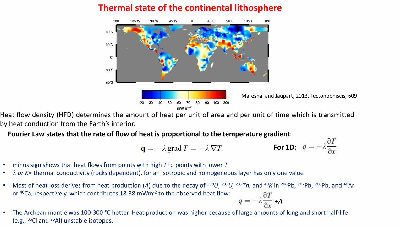
Thermal state of the continental lithosphere

• Most of heat loss derives from heat production (A) due to the decay of 238U, 235U, 232Th, and 40K in 206Pb, 207Pb, 208Pb, and 40Aror 40Ca, respectively, which contributes 18-38 mWm-2 to the observed heat flow:

• The Archean mantle was 100-300 °C hotter. Heat production was higher because of large amounts of long and short half-life (e.g., 36Cl and 26Al) unstable isotopes.

Heat flow density (HFD) determines the amount of heat per unit of area and per unit of time which is transmittedby heat conduction from the Earth’s interior.

Fourier Law states that the rate of flow of heat is proportional to the temperature gradient:

• minus sign shows that heat flows from points with high T to points with lower T• l or K= thermal conductivity (rocks dependent), for an isotropic and homogeneous layer has only one value

For 1D:

Mareshal and Jaupart, 2013, Tectonophiscis, 609

+A

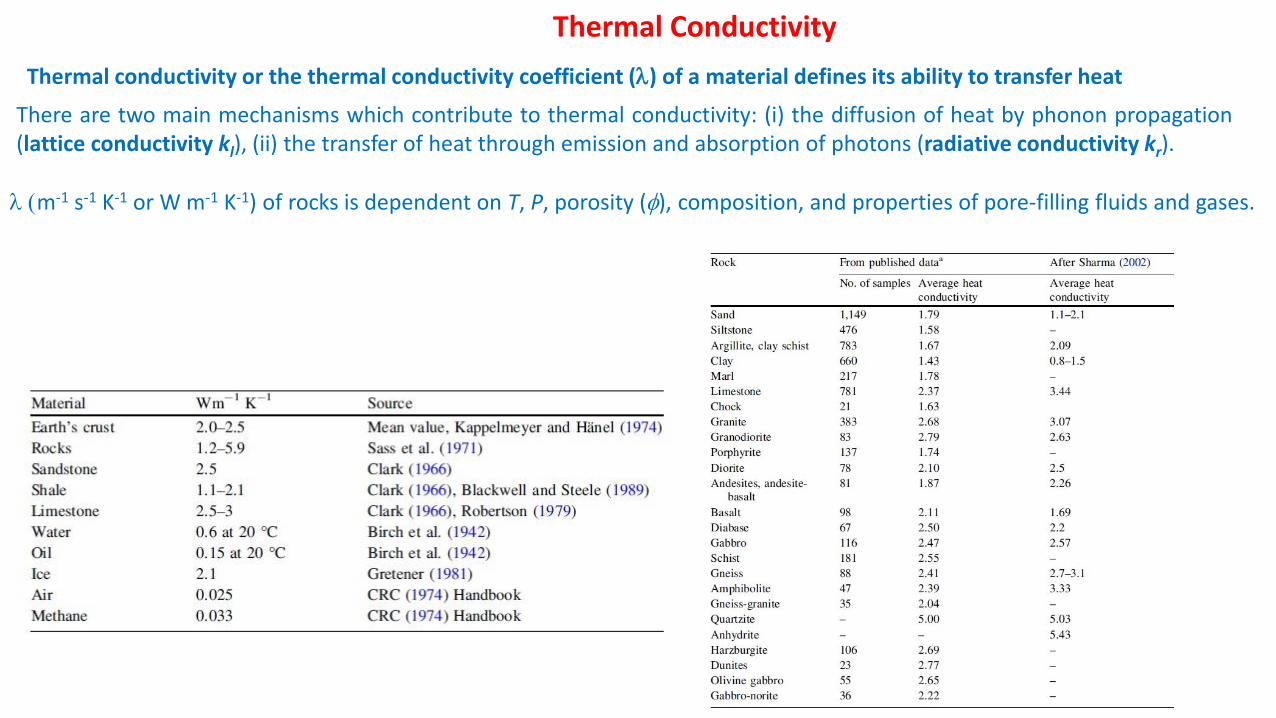
Thermal conductivity or the thermal conductivity coefficient (l) of a material defines its ability to transfer heat

Thermal Conductivity

There are two main mechanisms which contribute to thermal conductivity: (i) the diffusion of heat by phonon propagation(lattice conductivity kl), (ii) the transfer of heat through emission and absorption of photons (radiative conductivity kr).

l (m-1 s-1 K-1 or W m-1 K-1) of rocks is dependent on T, P, porosity (f), composition, and properties of pore-filling fluids and gases.

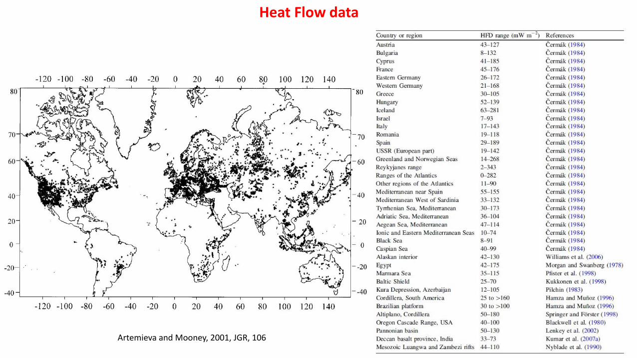
Heat Flow data

Artemieva and Mooney, 2001, JGR, 106

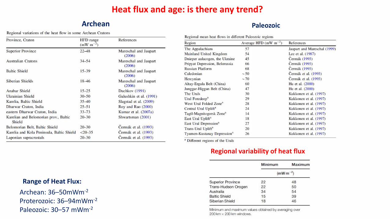
Heat flux and age: is there any trend?

Archean Paleozoic

Archean: 36–50mWm-2

Proterozoic: 36–94mWm-2

Paleozoic: 30–57 mWm-2

Range of Heat Flux:

Regional variability of heat flux

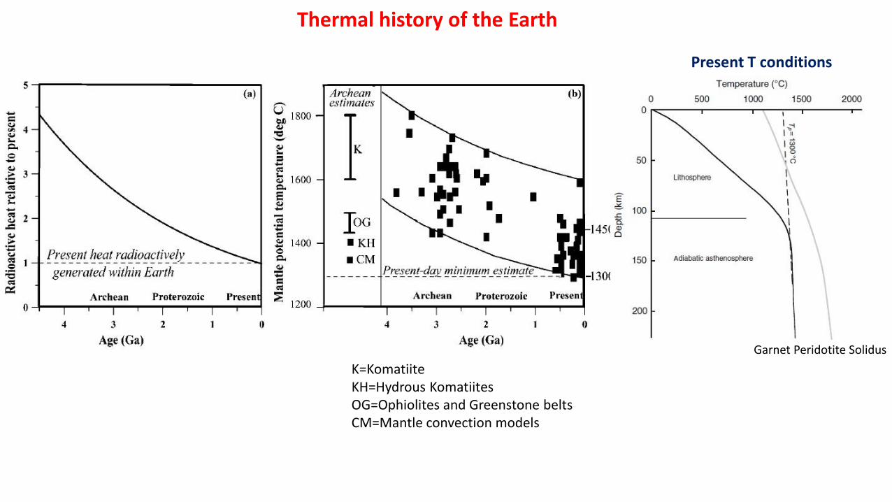
Thermal history of the Earth

K=KomatiiteKH=Hydrous KomatiitesOG=Ophiolites and Greenstone beltsCM=Mantle convection models

Garnet Peridotite Solidus

Present T conditions

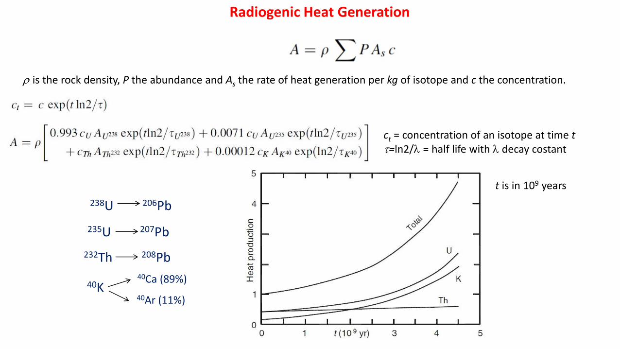
Radiogenic Heat Generation

ct = concentration of an isotope at time tt=ln2/l = half life with l decay costant

t is in 109 years

is the rock density, P the abundance and As the rate of heat generation per kg of isotope and c the concentration.

235U 207Pb

40K

232Th 208Pb

238U 206Pb

40Ar (11%)

40Ca (89%)

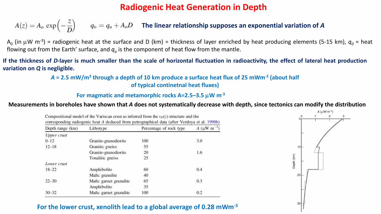
Radiogenic Heat Generation in Depth

A0 (in mW m-3) = radiogenic heat at the surface and D (km) = thickness of layer enriched by heat producing elements (5-15 km), q0 = heatflowing out from the Earth’ surface, and qa is the component of heat flow from the mantle.

For magmatic and metamorphic rocks A=2.5–3.5 mW m-3

A = 2.5 mW/m3 through a depth of 10 km produce a surface heat flux of 25 mWm-2 (about half of typical continetnal heat fluxes)

For the lower crust, xenolith lead to a global average of 0.28 mWm-3

Measurements in boreholes have shown that A does not systematically decrease with depth, since tectonics can modify the distribution

If the thickness of D-layer is much smaller than the scale of horizontal fluctuation in radioactivity, the effect of lateral heat productionvariation on Q is negligible.

The linear relationship supposes an exponential variation of A

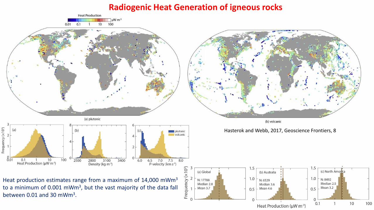
Radiogenic Heat Generation of igneous rocks

Hasterok and Webb, 2017, Geoscience Frontiers, 8

Heat production estimates range from a maximum of 14,000 mWm3

to a minimum of 0.001 mWm3, but the vast majority of the data fallbetween 0.01 and 30 mWm3.

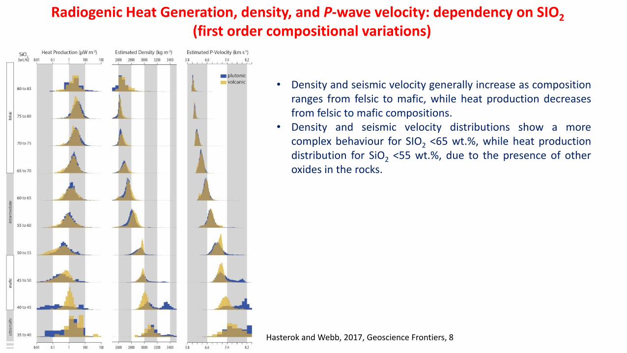
Radiogenic Heat Generation, density, and P-wave velocity: dependency on SIO2

(first order compositional variations)

• Density and seismic velocity generally increase as compositionranges from felsic to mafic, while heat production decreasesfrom felsic to mafic compositions.

• Density and seismic velocity distributions show a morecomplex behaviour for SIO2 <65 wt.%, while heat productiondistribution for SiO2 <55 wt.%, due to the presence of otheroxides in the rocks.

Hasterok and Webb, 2017, Geoscience Frontiers, 8

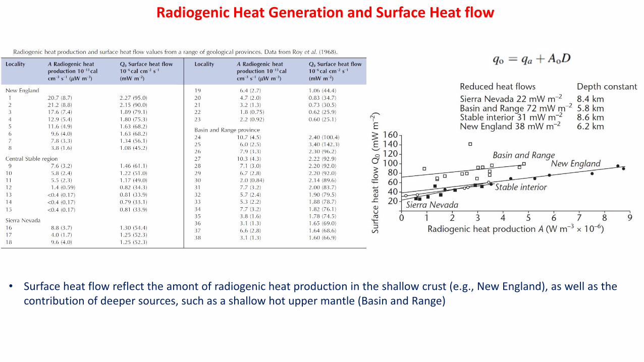
Radiogenic Heat Generation and Surface Heat flow

• Surface heat flow reflect the amont of radiogenic heat production in the shallow crust (e.g., New England), as well as thecontribution of deeper sources, such as a shallow hot upper mantle (Basin and Range)

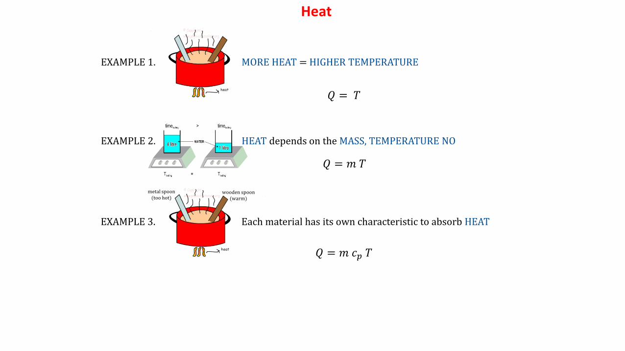
EXAMPLE 1. MORE HEAT = HIGHER TEMPERATURE

EXAMPLE 2. HEAT depends on the MASS, TEMPERATURE NO

EXAMPLE 3. Each material has its own characteristic to absorb HEAT

metal spoon (too hot)

wooden spoon (warm)

𝑄 = 𝑚 𝑐𝑝 𝑇

𝑄 = 𝑇

𝑄 = 𝑚 𝑇

Heat

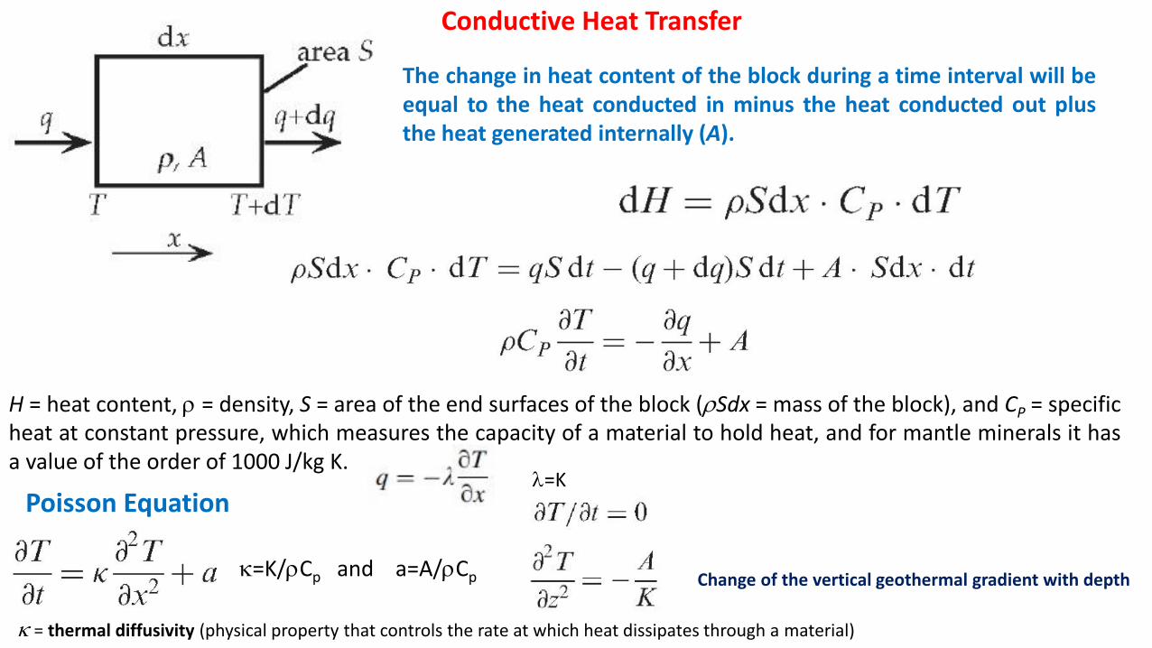
H = heat content, = density, S = area of the end surfaces of the block (Sdx = mass of the block), and CP = specificheat at constant pressure, which measures the capacity of a material to hold heat, and for mantle minerals it hasa value of the order of 1000 J/kg K.

Conductive Heat Transfer

The change in heat content of the block during a time interval will beequal to the heat conducted in minus the heat conducted out plusthe heat generated internally (A).

k=K/Cp and a=A/Cp

Poisson Equation

Change of the vertical geothermal gradient with depth

l=K

k = thermal diffusivity (physical property that controls the rate at which heat dissipates through a material)

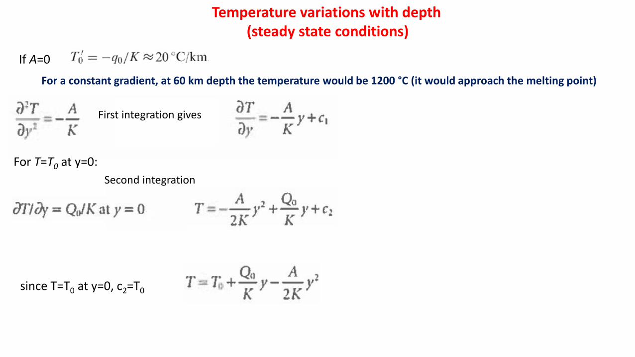
Temperature variations with depth(steady state conditions)

First integration gives

For T=T0 at y=0:

Second integration

since T=T0 at y=0, c2=T0

If A=0

For a constant gradient, at 60 km depth the temperature would be 1200 °C (it would approach the melting point)

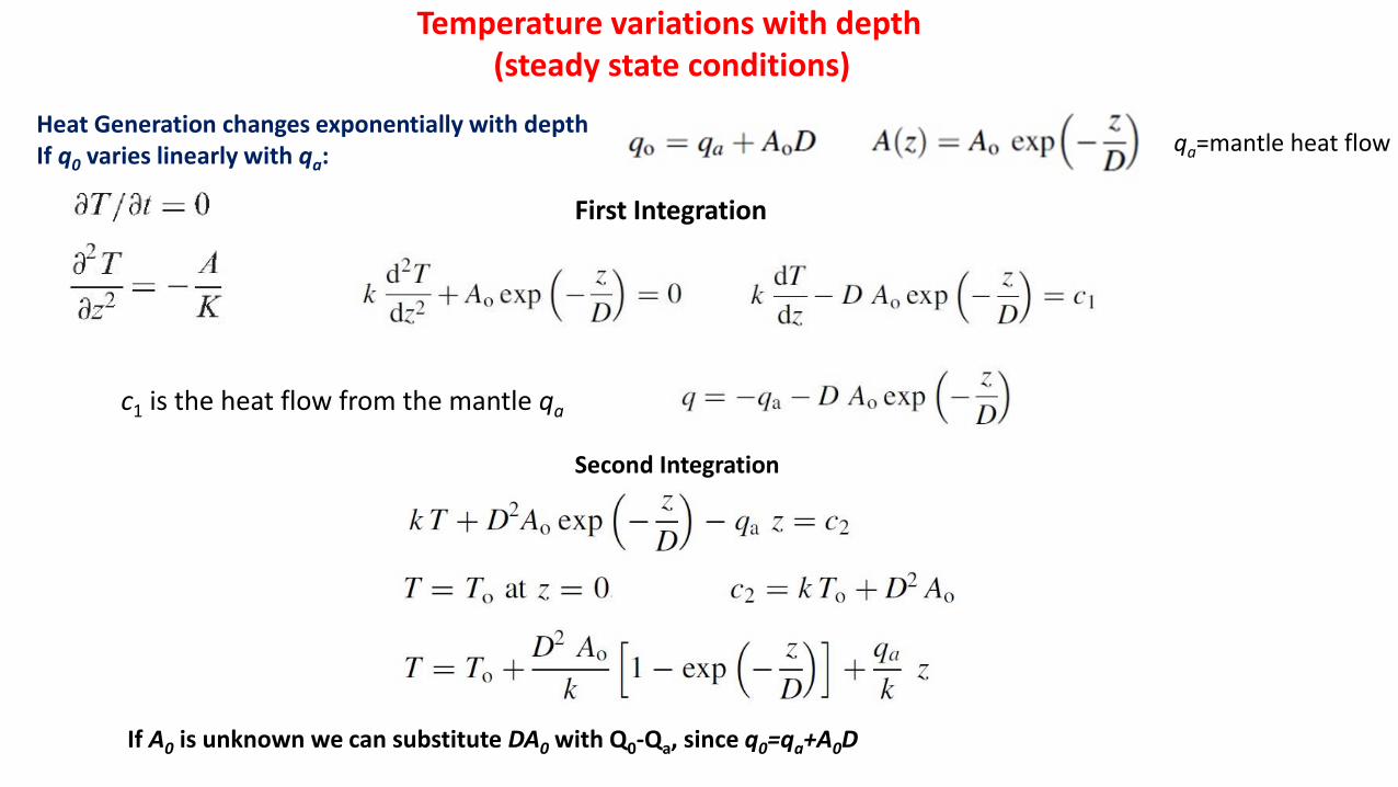
Temperature variations with depth(steady state conditions)

c1 is the heat flow from the mantle qa

If A0 is unknown we can substitute DA0 with Q0-Qa, since q0=qa+A0D

Heat Generation changes exponentially with depthIf q0 varies linearly with qa:

First Integration

Second Integration

qa=mantle heat flow

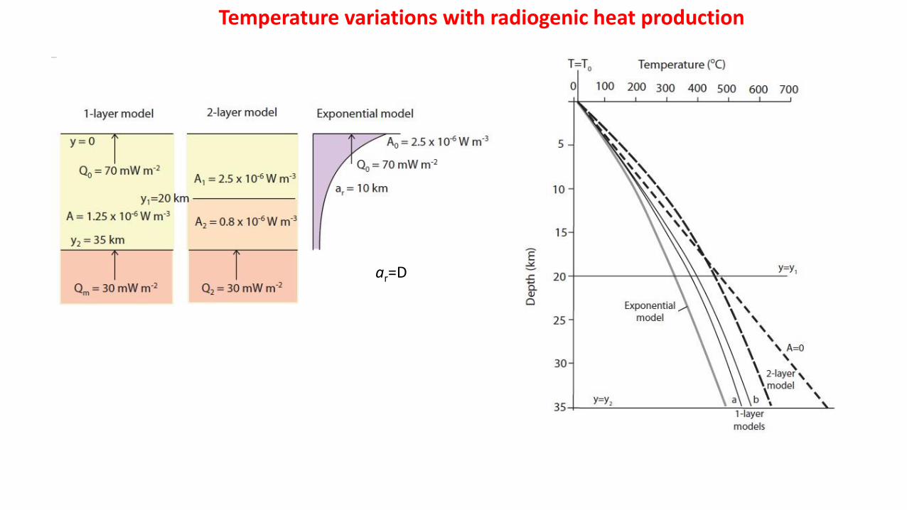
Temperature variations with radiogenic heat production

ar=D

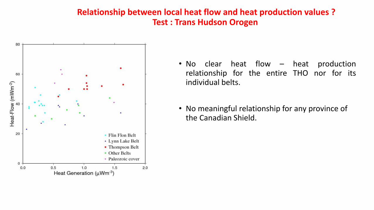
Relationship between local heat flow and heat production values ?Test : Trans Hudson Orogen

• No clear heat flow – heat productionrelationship for the entire THO nor for itsindividual belts.

• No meaningful relationship for any province of the Canadian Shield.

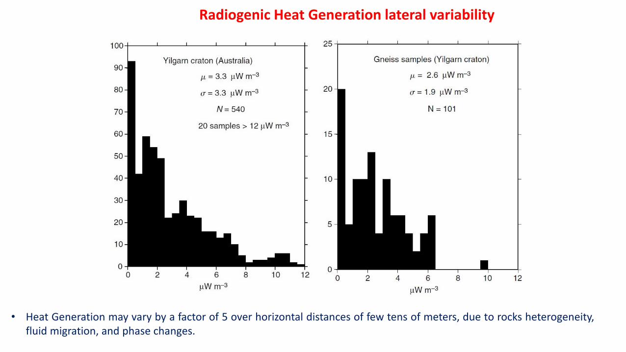
Radiogenic Heat Generation lateral variability

• Heat Generation may vary by a factor of 5 over horizontal distances of few tens of meters, due to rocks heterogeneity,fluid migration, and phase changes.

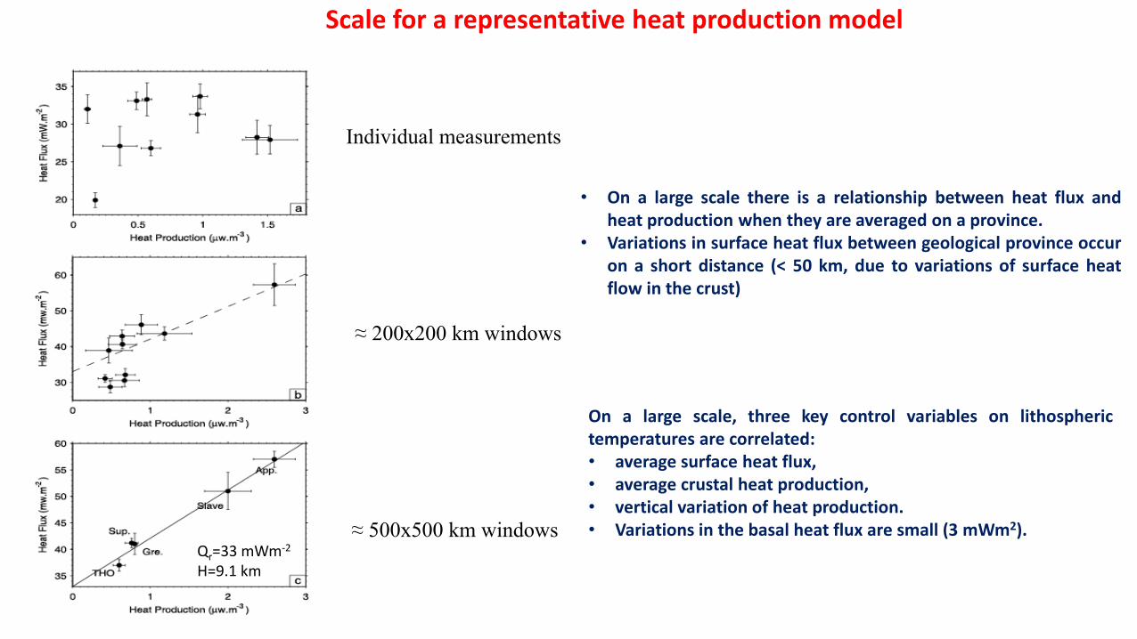
Scale for a representative heat production model

Individual measurements

≈ 200x200 km windows

≈ 500x500 km windows

On a large scale, three key control variables on lithospherictemperatures are correlated:• average surface heat flux,• average crustal heat production,• vertical variation of heat production.• Variations in the basal heat flux are small (3 mWm2).

• On a large scale there is a relationship between heat flux andheat production when they are averaged on a province.

• Variations in surface heat flux between geological province occuron a short distance (< 50 km, due to variations of surface heatflow in the crust)

Qr=33 mWm-2

H=9.1 km

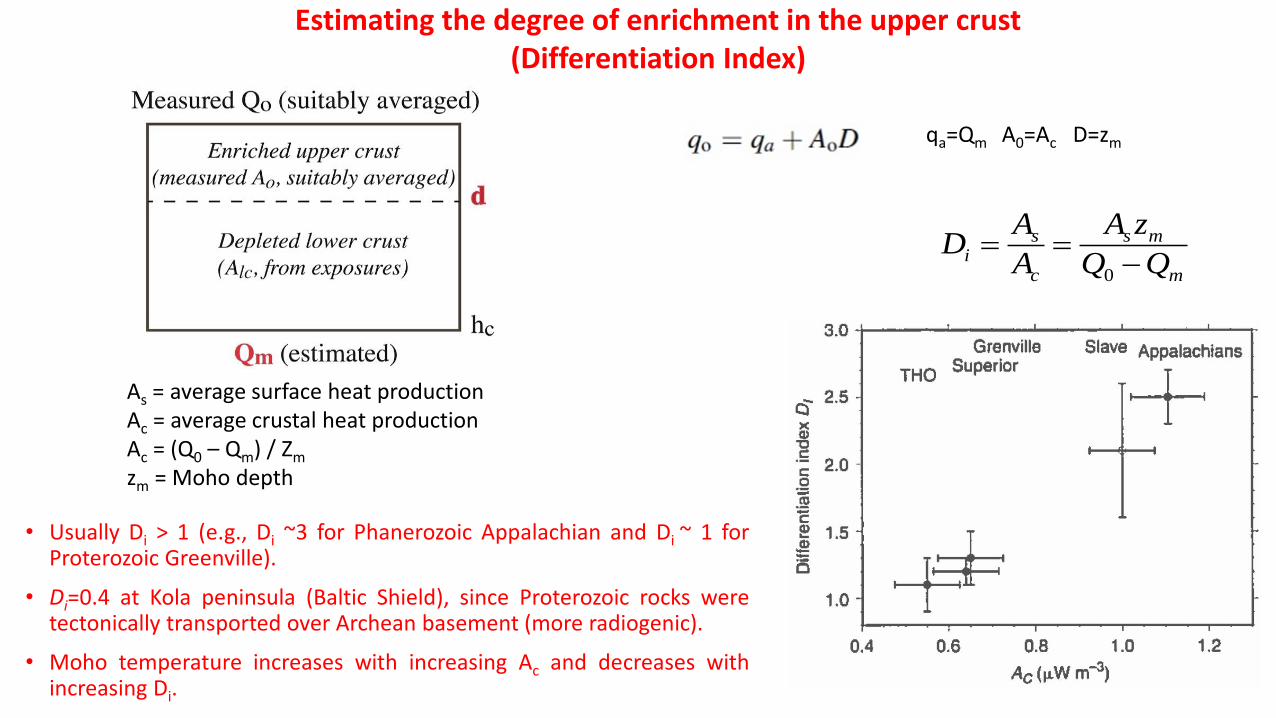
• Usually Di > 1 (e.g., Di ~3 for Phanerozoic Appalachian and Di ~ 1 forProterozoic Greenville).

• Di=0.4 at Kola peninsula (Baltic Shield), since Proterozoic rocks weretectonically transported over Archean basement (more radiogenic).

• Moho temperature increases with increasing Ac and decreases withincreasing Di.

m

ms

c

si QQ

zA

A

AD

0

Estimating the degree of enrichment in the upper crust(Differentiation Index)

As = average surface heat productionAc = average crustal heat productionAc = (Q0 – Qm) / Zm

zm = Moho depth

qa=Qm A0=Ac D=zm

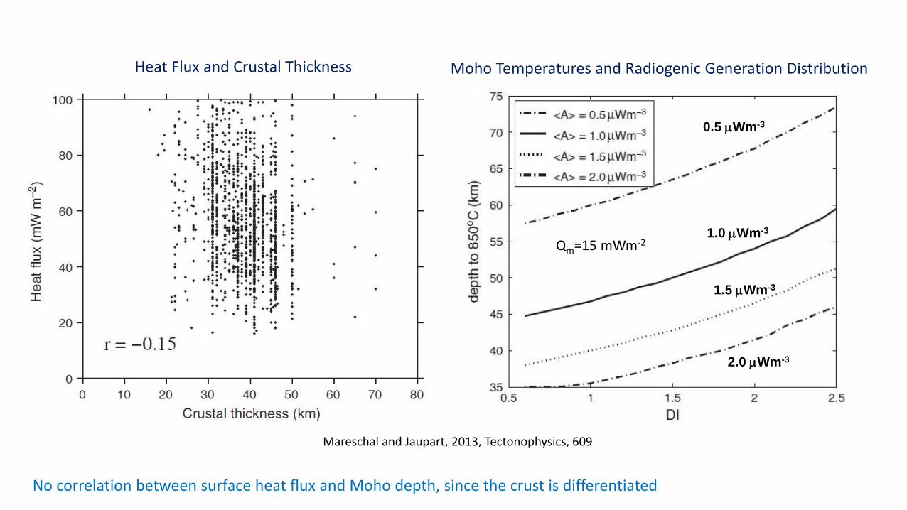
Moho Temperatures and Radiogenic Generation Distribution

0.5 mWm-3

2.0 mWm-3

1.0 mWm-3

1.5 mWm-3

Qm=15 mWm-2

Mareschal and Jaupart, 2013, Tectonophysics, 609

No correlation between surface heat flux and Moho depth, since the crust is differentiated

Heat Flux and Crustal Thickness

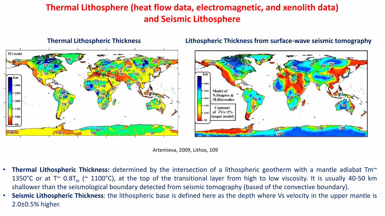
Thermal Lithosphere (heat flow data, electromagnetic, and xenolith data)and Seismic Lithosphere

Thermal Lithospheric Thickness

• Thermal Lithospheric Thickness: determined by the intersection of a lithospheric geotherm with a mantle adiabat Tm~1350°C or at T~ 0.8Tm (~ 1100°C), at the top of the transitional layer from high to low viscosity. It is usually 40-50 kmshallower than the seismological boundary detected from seismic tomography (based of the convective boundary).

• Seismic Lithospheric Thickness: the lithospheric base is defined here as the depth where Vs velocity in the upper mantle is2.0±0.5% higher.

Lithospheric Thickness from surface-wave seismic tomography

Artemieva, 2009, Lithos, 109

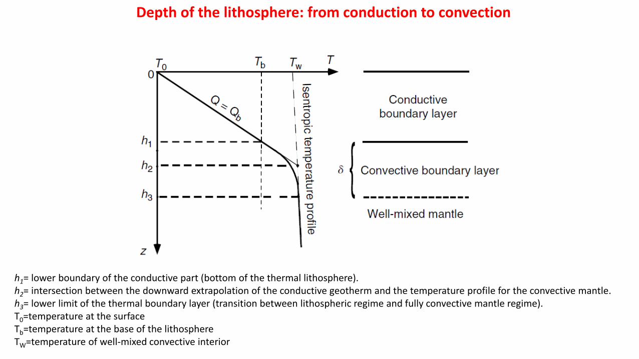
h1= lower boundary of the conductive part (bottom of the thermal lithosphere).h2= intersection between the downward extrapolation of the conductive geotherm and the temperature profile for the convective mantle.h3= lower limit of the thermal boundary layer (transition between lithospheric regime and fully convective mantle regime).T0=temperature at the surfaceTb=temperature at the base of the lithosphereTW=temperature of well-mixed convective interior

Depth of the lithosphere: from conduction to convection

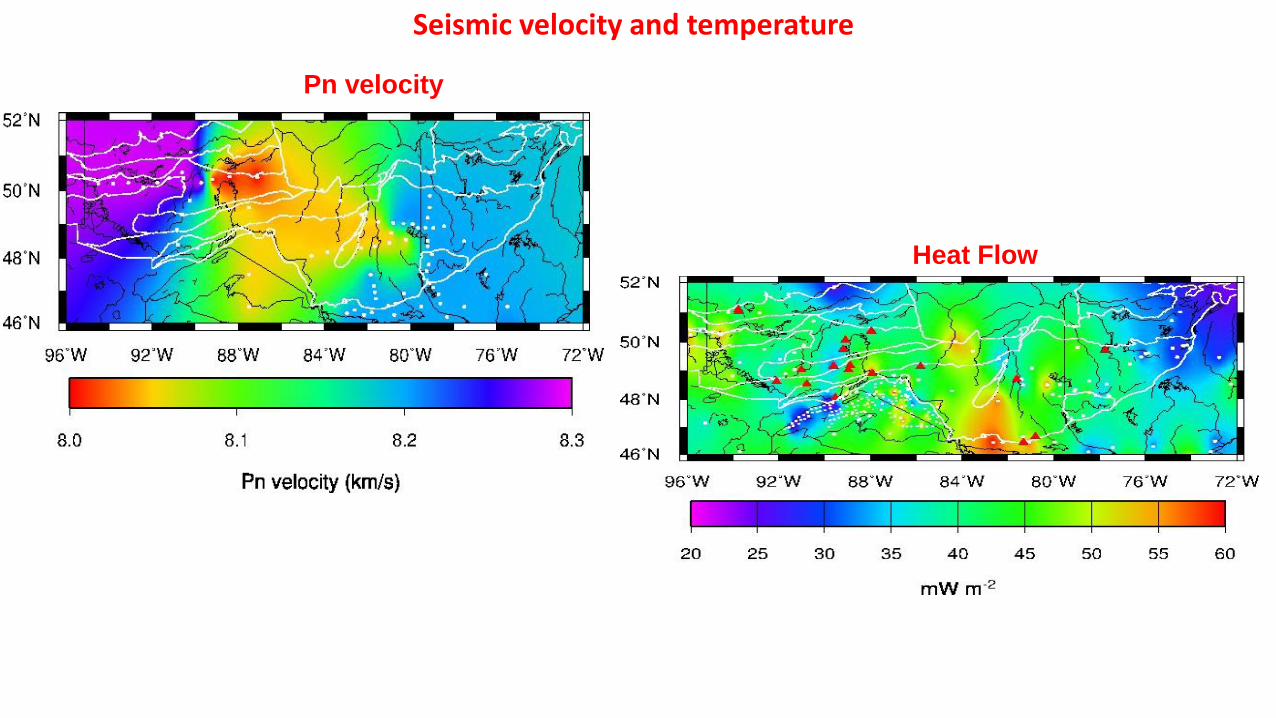
Pn velocity

Heat Flow

Seismic velocity and temperature

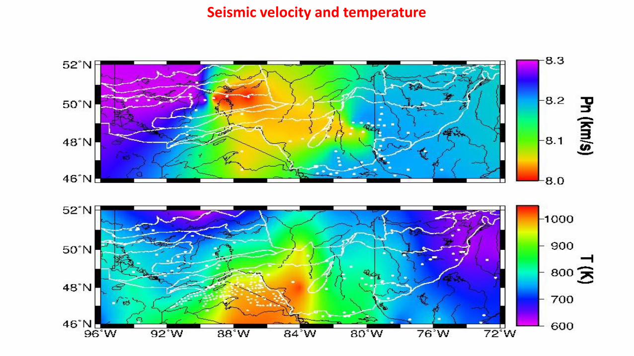
Seismic velocity and temperature

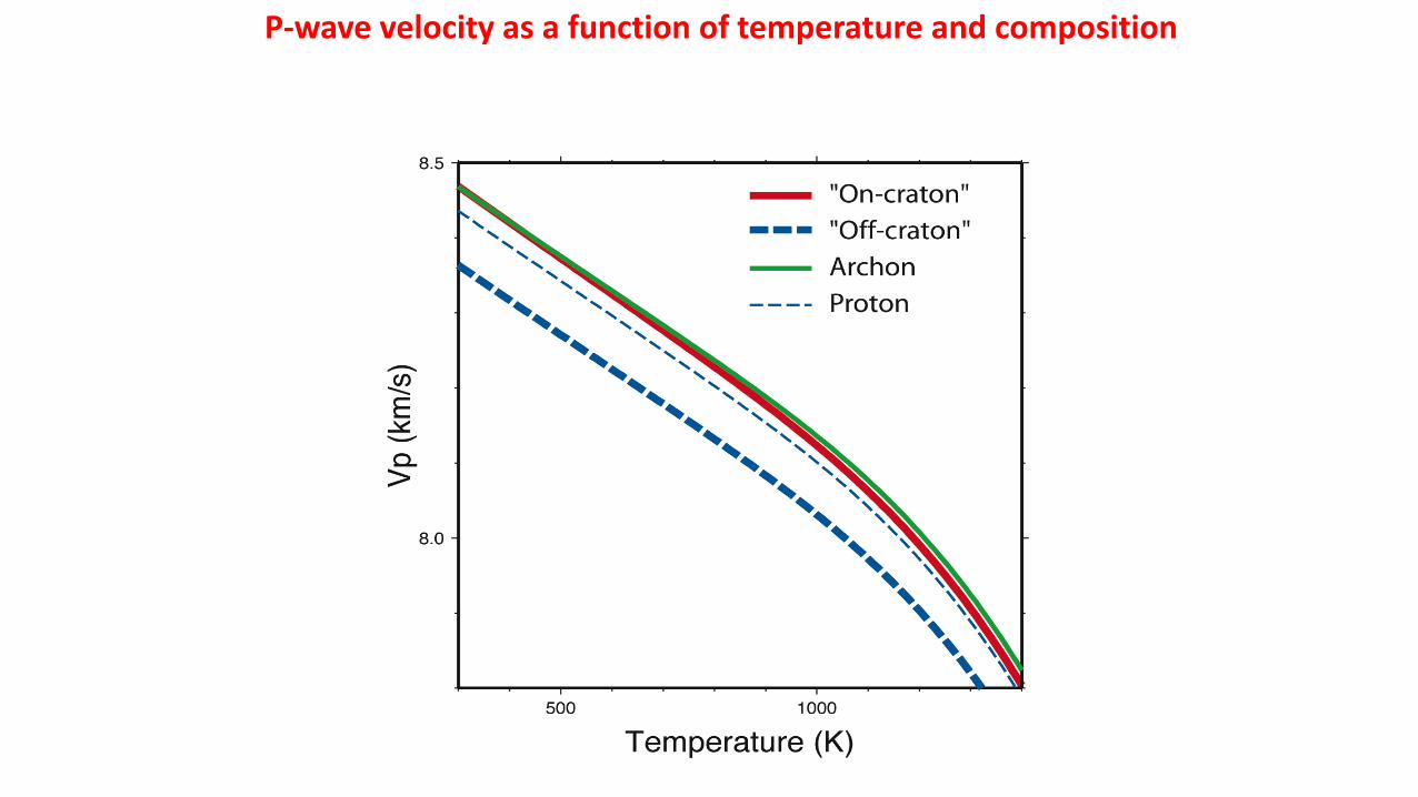
P-wave velocity as a function of temperature and composition

75

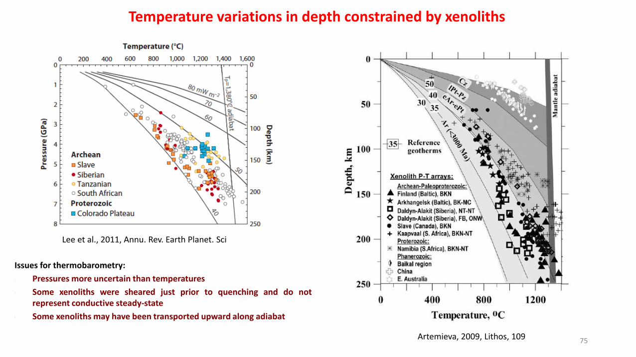
Lee et al., 2011, Annu. Rev. Earth Planet. Sci

Artemieva, 2009, Lithos, 109

Issues for thermobarometry:

l Pressures more uncertain than temperatures

l Some xenoliths were sheared just prior to quenching and do notrepresent conductive steady-state

l Some xenoliths may have been transported upward along adiabat

Temperature variations in depth constrained by xenoliths

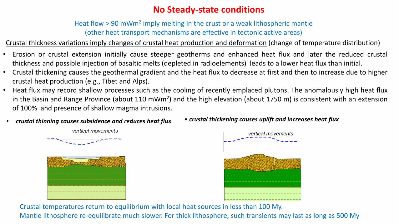
Heat flow > 90 mWm2 imply melting in the crust or a weak lithospheric mantle (other heat transport mechanisms are effective in tectonic active areas)

No Steady-state conditions

Crustal thickness variations imply changes of crustal heat production and deformation (change of temperature distribution)

• Erosion or crustal extension initially cause steeper geotherms and enhanced heat flux and later the reduced crustalthickness and possible injection of basaltic melts (depleted in radioelements) leads to a lower heat flux than initial.

• Crustal thickening causes the geothermal gradient and the heat flux to decrease at first and then to increase due to highercrustal heat production (e.g., Tibet and Alps).

• Heat flux may record shallow processes such as the cooling of recently emplaced plutons. The anomalously high heat fluxin the Basin and Range Province (about 110 mWm2) and the high elevation (about 1750 m) is consistent with an extensionof 100% and presence of shallow magma intrusions.

Crustal temperatures return to equilibrium with local heat sources in less than 100 My.Mantle lithosphere re-equilibrate much slower. For thick lithosphere, such transients may last as long as 500 My

vertical movements

• crustal thinning causes subsidence and reduces heat flux • crustal thickening causes uplift and increases heat flux