Coupled Rotor-Fuselage Analysis with Finite Motions

Using Component Mode Synthesis∗

Olivier A. Bauchau and Jesus RodriguezSchool of Aerospace Engineering,Georgia Institute of Technology,

Atlanta, GA, USA.Shyi-Yaung Chen

Research and Engineering,Sikorsky Aircraft, Stratford, CT, USA.

Abstract

This paper is concerned with the modeling of a rotor-fuselage system undergoing large anglemaneuvers. The behavior of the elastic fuselage will be represented by a modal approximation,thereby greatly reducing the computational cost of the simulation. In this work, a floatingframe approach is used. The total motion of the fuselage consists of the superposition of therigid body motions of the floating frame and of elastic motions that are assumed to remainsmall. The proposed formulation makes use of a component mode synthesis technique thatleaves the analyst free to choose any type of modal basis and simplifies the connection of thefuselage to other rotorcraft components. The proposed formulation is independent of the finiteelement analysis package used to compute the modes of the fuselage. It is also shown that inthe absence of elastic deformations, the formulation recovers the exact equations of motion fora rigid body.

1 Introduction

Rotorcraft vibration analyses often assume the hub to be attached to an inertial point. While thisconvenient approximation considerably simplifies the analysis, it implies that rotor and fuselageresponses are fully decoupled. In reality, airframe motion is known to have a significant impact onhub loads, see Refs. [1, 2]. Consequently, a comprehensive rotorcraft dynamics analysis requiresthe coupling of a realistic fuselage model to a nonlinear rotor model. Helicopters and tilt-rotorsperform complex, highly dynamic and often three-dimensional maneuvers, both in normal operatingconditions and during emergencies. The ability to perform aggressive and violent maneuvers isclearly a primary goal of rotorcraft systems designed for military applications. In fact, limits onthe maneuvers a rotorcraft can fly might arise not from the ability of the rotor system to generatethe desired thrust, but on the ability of critical dynamic components to carry the resulting loads.Hence, coupled rotor/fuselage models are needed for hover, forward flight, and maneuvers.

Various methods have been proposed for the study of rotor-fuselage interactions. The impedancematching method was implemented to couple and solve rotor and fuselage dynamics (Refs. [3, 4]).Reference [5] derived a set of dynamic equations of motion for a rotor-fuselage system which was

∗Journal of the American Helicopter Society, 49(2), pp 201– 211, 2004

1

solved by means of the harmonic balance technique. Stephens and Peters (Ref. [6]) presented bothan iterative method and a fully coupled method to predict the response a rotor-body system. Birand Chopra (Ref. [7]) studied the dynamic response of a rotor/rigid fuselage system subjected to athree-dimensional gust. References [8, 2] derived a comprehensive set of rotor-body equations forthe analysis of the Bell AH-1G helicopter. Many of these approaches assume small amplitude rigidbody motions of the fuselage, rendering them inapplicable to large angle maneuver flights. Othertechniques require the reformulation of the blade equations of motion, a cumbersome task. Modalapproximation seems to be the method of choice for representing the elasticity of the fuselage,leading to manageable computational costs. The diversity of the approaches and their underlyingassumptions underscore the difficulties associated with the formulation and solution of this complexproblem.

Modal based approximations of complex elastic substructures have been widely used withinthe framework of multibody dynamics. One of the most common approaches is based on theconcept of floating frames (Refs. [9, 10]) whereby the total motion of a flexible body is broken intotwo parts: rigid body motions represented by the motion of the floating frame, and superimposed“elastic motions.” This decomposition allows the introduction of simplifying assumptions: althoughthe total motion is always finite, the elastic motions remain small. In forward flight, the rigidbody motion simply is a forward translation, but in maneuver flight, large angle motion will beencountered. In both cases, elastic motions are assumed to be small. The focus of this paper is theformulation of modal based elements that can be used to model coupled rotor/fuselage problemsin hover, forward flight and maneuvers, within the framework of finite element based, nonlinearflexible multibody dynamics formulations.

Although the concept of floating frame is rather intuitive, the implementation of a computationalprocedure based on this idea must deal with several thorny issues. First, the accuracy of the analysiswill critically depend on the selection of a suitable modal basis. Second, a specific floating framemust be selected: it could be attached to a point of the elastic body or moving with respect toit. Third, the modal based elements should be easy to couple with the other components of thesystem modeled with multibody formulations. This points towards the use of component modesynthesis techniques that are well developed for structural dynamics problems. Fourth, in theabsence of elastic deformations, the formulation should recover the exact equations of motion for arigid body. Finally, the formulation should be independent of the finite element analysis packageused to compute the modes of the elastic components; any commercial finite element package couldbe used, and the resulting modal based element can be used independently of the commercialpackage. These various issues will be discussed in more detail in the following paragraphs.

The first critical step is the selection of a suitable modal basis. Ideally, the selected modesshould capture as accurately as possible the deformation patterns encountered during flight. Con-sequently, the analyst should be given the greatest possible freedom to select appropriate modes.The formulation should not put any restriction on the choice of the modal basis. In particular,the modes near integer multiples of the blade passage frequency should be included in the analysis.Since such modes will not be the lowest frequency modes of the fuselage, a highly detailed finiteelement model must be used. The DAMVIBS program (Ref. [11]) describes the results of some ofthe research efforts in this area.

Next, a specific floating frame must be selected. Since there exists no unique manner of definingthe “rigid” and “elastic” motions, the floating frame can be selected in a number of different ways.Several authors make use of body-attached frames, i.e. the floating frame is attached to an arbitrarypoint in the body (Refs. [12, 13, 14]). Other authors rely on floating frames moving with respect tothe elastic body (Refs. [15, 16]). Since the choice of the location of the moving frame is not unique,a specific condition must be selected to remove this indeterminacy. For instance, one can chooseto minimize the kinetic energy (Ref. [15]), to place the frame at the mass center of the structure(Ref. [16]), or follow the center-of-mass/mean axis convention used for rotorcraft modeling (Ref. [5]).

2

The choice of one condition or the other seems to be a matter of computational convenience. Themoving frame approach seems to be more desirable than the body-attached approach because iteliminates the need to arbitrarily select a material point where to attach the floating frame. On theother hand, the moving frame approach also involves the analyst’s insight since a specific conditionmust be selected to determine its location. Furthermore, this latter approach comes at the expenseof additional computational complexity. In this work, a body-attached frame will be used.

In some formulations, the choice of the floating frame is intimately linked to that of the modesused in the reduction technique (Refs. [17, 18, 9]). This linkage hinders the selection of the mostappropriate modes because the boundary conditions used to compute them do not necessarily matchthose of the flexible component once it is part of a multibody system.

An important issue in the formulation is the coupling of the modal based element representingthe fuselage to the rotor, tail rotor and landing gear. In the classical application of modal analysis(Ref. [19]), the displacement field is represented as a linear combination of mode shapes. This typeof representation has been used by some authors (Ref. [20]) in the context of multibody dynamicsanalysis, but it requires special techniques for coupling the modal based element with the othercomponents of the system. Typically, this is done by formulating a constraint condition that equatesthe modal superposition to the physical displacement at a node of the model (Ref. [21]). However,this approach does not take advantage of the component mode synthesis techniques that have beendeveloped for structural dynamics problems over the past thirty years. In these approaches, themodel of the fuselage involves two types of degrees of freedom: physical degrees of freedom ata limited number of connection points (called “boundary nodes”) and modal degrees of freedomrepresenting its internal flexibility. The fuselage is then readily connected at the boundary nodesto the main and tail rotors or landing gear without resorting to complex coupling techniques.Among the most widely used component mode synthesis techniques are those of Craig and Bampton(Ref. [22]), MacNeal (Ref. [23]), Rubin (Ref. [24]). Other efforts include those of Herting (Ref. [25]),Hintz (Ref. [26]) and refinements of the Craig-Bampton method (Ref. [27]).

Component mode synthesis methods were first used in the context of multibody dynamics byHaug and coworkers (Refs. [28, 29, 30, 31]) and later by Cardona and coworkers (Refs. [13, 14,16]) who used the Craig-Bampton method. Unfortunately, this method requires the use of modesassociated with clamped conditions at the boundary nodes: i.e. the modal basis must be selectedamong the modes of the fuselage clamped at the main and tail rotor connections and landing gearconnection. This would clearly lead to a poor representation of fuselage flexibility. This fundamentallimitation of the approach was recognized by Craig and Bampton who suggested the use of “staticcorrection modes” to alleviate the problem. It also prompted the development of the MacNeal-Rubin method. However, in this case, free conditions must be used at all boundary nodes: themodal basis must be select from among the modes of the unconstrained fuselage excluding the mainand tail rotors and landing gear. Furthermore, this method is more cumbersome to implementthan the Craig-Bampton method; it seems that the MacNeal-Rubin method has not been used inconjunction with multibody formulations. Finally, Herting’s method offers a more general approachthat enables the analyst to choose any type of modes. In fact, predictions based on the Craig-Bampton and MacNeal-Rubin methods were found to be in good agreement with those obtainedfrom Herting’s method (Ref. [25]). In this work, Herting’s method will be used as it provides theanalyst maximum flexibility.

The formulation of modal based elements should be independent of the finite element analysispackage used to compute the modes of the elastic components (Refs. [28, 29, 13, 14, 16]). This meansthat the computation of the mass and stiffness coefficients used for the formulation of a modal basedelement should be solely based on the information readily provided by the finite element package.Typically, rotorcraft companies develop very sophisticated fuselage models using commercial finiteelement packages (Ref. [11]); these models involve hundreds of thousands of degrees of freedom. Theformulation of the modal based element should require some basic information provided by these

3

models, such as the linearized mass and stiffness matrices, but it should not require additional data.Some formulations have been proposed in which the finite element analysis tool is embedded in themultibody formulation (Ref. [32]). Although higher accuracy can be achieved in that manner, thisis clearly not a practical option when a realistic finite element model of a fuselage is used. Yoo andHaug (Ref. [28, 29]) showed that by assuming a lumped mass representation of the elastic body, themodal based formulation could be fully decoupled from the finite element package. Unfortunately,the lumped mass approximation is rarely used for realistic fuselage models. Cardona and Geradin(Refs. [13, 14, 16]) used a corotational technique to achieve the same decoupling without resortingto the lumped mass approximation.

The proposed modal based element for fuselage dynamics modeling is fully independent of thefinite element analysis package. The mass and stiffness coefficients of the element are computed onthe sole basis of the unconstrained mass and stiffness matrices of the elastic fuselage and Herting’stransformation. Existing finite element models of fuselages can be readily used to generate themodal based element. It is also shown that Herting’s transformation applies to the inertial velocitiesrequired to compute the kinetic energy of the elastic component, under the sole assumption of smalldisplacements.

The paper is organized in the following manner. After a brief discussion of the notational con-ventions used in this work, the component mode synthesis technique presented by Herting (Ref. [25])is briefly reviewed. Next, the modal based multibody formulation is described. Finally, the lastsection presents numerical examples to validate the proposed formulation.

2 Notational Conventions

The kinematic description of bodies in their reference and deformed configurations will make useof three orthonormal bases. First, an inertial basis is used as a global reference for the system; itis denoted I := (ı1, ı2, ı3), the over-bar indicates a unit vector. A second basis B0 := (e01, e02, e03),is attached to the body and defines its orientation in the reference configuration. Finally, a thirdbasis B := (e1, e2, e3) defines the orientation of the body in its deformed configuration.

Let u0 and u (under-bars indicate vector quantities) be the displacement vectors from I to B0

and B0 to B, respectively, and R0 and R the rotation tensors from I to B0 and B0 to B, respectively.In this work, all vector and tensor components are measured in either I or B. For instance, thecomponents of vector u measured in I, and B will be denoted u, and u∗, respectively, and clearly

u∗ = (RR0)T u. (1)

Similarly, the components of tensor R measured in I and B will be denoted R and R∗, respectively.The notation (.)T denotes the transposition of a vector of matrix. The skew-symmetric matrixformed with the components u will be denoted u

u =

0 −u3 u2u3 0 −u1−u2 u1 0

. (2)

3 Herting’s Transformation

Consider an elastic fuselage whose linearized equations of motion are in the following form

M ¨u∗ +Ku∗ = F (t), (3)

where u∗(t) is the array of nodal displacements and rotations, F (t) the array of externally appliednodal forces, K and M the unconstrained stiffness and mass matrices of the fuselage, respectively,

4

and t time. The notation (.) is used to denote the nodal values of quantities discretized using finiteelement procedures. For three dimensional problems, matrix K is six times singular, correspondingto the six rigid body modes of the fuselage. The structure is assumed to be undamped or lightlydamped and hence, damping effects are neglected. Eqs. (3) forms a large set of N algebraic equa-tions, typically obtained from a spatial discretization process such as the finite element method. Letmatrix P store all the mass normalized eigenmodes of the fuselage in order of ascending frequencies

P = [PR, PE] , (4)

where PR =[

u1, u2, . . . uNR

]

stores the NR rigid body modes of the structure and PE =[

uNR+1, uNR+2, . . . uN]

its N −NR elastic modes.The aim of this work is to develop a modal approximation to the elastic component (fuselage)

represented by eqs. (3) which will be connected to other components (main and tail rotor, land-ing gear) to form the complete system (rotorcraft) to be analyzed. The other components could bemodeled by a modal representation, or by a multibody formulation. In order to allow the connectionof a specific component to others, its degrees of freedom will be partitioned into boundary and inte-rior degrees of freedom, denoted dB∗ and uI∗, respectively. The array dB∗T = ⌊dB∗T

1 , dB∗T2 , . . . dB∗T

m ⌋stores the six degrees of freedom for each of the m boundary points of the component. Each bound-ary point requires six degrees of freedom, three displacements and three rotations, for compatibilitywith multibody formulations, i.e. dB∗T

i = ⌊uB∗Ti , θB∗T

i ⌋. The following partition of the structuralmatrices is performed

M =

[

MBB MBI

M IB M II

]

; K =

[

KBB KBI

KIB KII

]

, (5)

u∗ =

[

dB∗

uI∗

]

; F (t) =

[

FB(t)

FI(t)

]

, (6)

and

PR =

[

PBR

P IR

]

; PE =

[

PBE

P IE

]

, (7)

where the superscripts (·)B and (·)I denoted the boundary and interior degrees of freedom, respec-tively. It is assumed that the partition KII is nonsingular.

Herting (Ref. [25]) introduced a coordinate transformation

u∗ = HH u, (8)

defined by a set of shape functions HH

HH =

[

I 0 0GIB HI

R P IE −GIBPB

E

]

, (9)

whereGIB = −KII−1KIB, (10)

HIR = −KII−1

(

M IB +M IIGIB)

PBR . (11)

The reduced set of degrees of freedom is

uT = ⌊dB∗T , qTR, qT

E⌋, (12)

where qR

and qE

correspond to the modal participation factors for the rigid and elastic modes,respectively.

5

In the absence of interior loads, i.e. when FI(t) = 0, the equations of motion, eqs. (3), reduce

toM ¨u+ K u = F , (13)

whereM = HT

HMHH ; K = HTHKHH ; F = HT

HF (t). (14)

Typically, boundary degrees of freedom and modal coordinates are coupled in the reduced massmatrix M , whereas the reduced stiffness matrix takes the following form

K =

[

KBB 00 Kqq

]

, (15)

where KBB is the partition obtained from a Guyan (Ref. [33]) reduction and the superscript (.)q

refers to the modal coordinates. Clearly, boundary degrees of freedom and modal coordinatesare statically uncoupled. In general, damping effect are not represented in finite element models;finite element codes provide a mass and a stiffness matrix but no damping matrix in eq. (3).Hence, component mode synthesis is typically performed for undamped systems. However, oncethe reduction has been performed to obtain the reduced mass and stiffness matrices, eq. (14), amodal damping matrix can be added to the model, often based on experimental measurements ofmodal damping.

4 Multibody Formulation

In this section, the kinematics of the modal based element are presented. The proposed formulationfollows the floating frame approach, where small elastic displacements and rotations are superim-posed with the large rigid body motion of the elastic body. Expressions for the kinetic and strainenergies are then derived.

4.1 Modal Based Element Kinematics

DeformedConfiguration

ReferenceConfiguration

P

i1

i2

i3

x0

F, R0

F

x0

P, R0

P

xF F, R

xP P, R

e0 1

F

e1

F

e0 1

P

e1

P

e0 2

F

e2

F

e0 2

P

e0 3

Fe0 3

F

e3

F

e0 3

P

e3

P e2

P

uP

sP

SP Fictitious

rigid bodyconfiguration

B0 F

BF

I

P

Figure 1: Configuration of the elastic body.

Consider the elastic body shown in Fig. 1. Theoverall rigid body motion of the elastic fuse-lage is described by a floating frame the ori-entation of which is defined by the orthonor-mal bases B0F :=

(

eF01, eF02, e

F03

)

and BF :=(

eF1 , eF2 , e

F3

)

in the reference and deformed con-figurations, respectively. Similarly, two addi-tional orthonormal bases define the orientationof a frame rigidly attached to the fuselage atan arbitrary point P, B0P :=

(

eP01, eP02, e

P03

)

andBP :=

(

eP1 , eP2 , e

P3

)

in the reference and de-formed configurations, respectively. RF

0 andRF are the components of the rotation tensorsfrom the inertial frame I to B0F and B0F toBF , respectively, both measured in I. Simi-larly, RP

0 and RP are the components of therotation tensors from I to B0P and B0P to BP ,respectively, both measured in I. In the ref-erence configuration, the origin of the floatingand body-attached frames are denoted by xF0

6

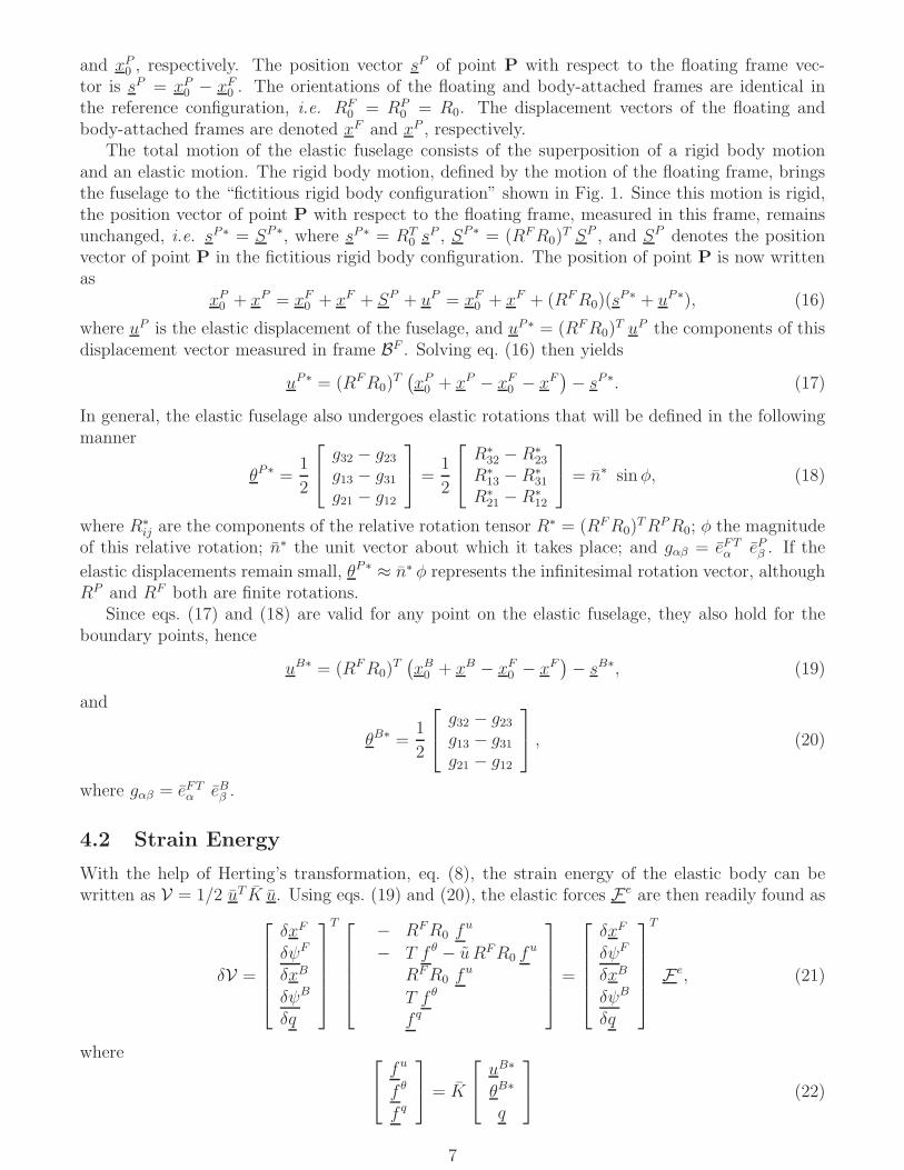
and xP0 , respectively. The position vector sP of point P with respect to the floating frame vec-tor is sP = xP0 − xF0 . The orientations of the floating and body-attached frames are identical inthe reference configuration, i.e. RF

0 = RP0 = R0. The displacement vectors of the floating and

body-attached frames are denoted xF and xP , respectively.The total motion of the elastic fuselage consists of the superposition of a rigid body motion

and an elastic motion. The rigid body motion, defined by the motion of the floating frame, bringsthe fuselage to the “fictitious rigid body configuration” shown in Fig. 1. Since this motion is rigid,the position vector of point P with respect to the floating frame, measured in this frame, remainsunchanged, i.e. sP∗ = SP∗, where sP∗ = RT

0 sP , SP∗ = (RFR0)

T SP , and SP denotes the positionvector of point P in the fictitious rigid body configuration. The position of point P is now writtenas

xP0 + xP = xF0 + xF + SP + uP = xF0 + xF + (RFR0)(sP∗ + uP∗), (16)

where uP is the elastic displacement of the fuselage, and uP∗ = (RFR0)T uP the components of this

displacement vector measured in frame BF . Solving eq. (16) then yields

uP∗ = (RFR0)T(

xP0 + xP − xF0 − xF)

− sP∗. (17)

In general, the elastic fuselage also undergoes elastic rotations that will be defined in the followingmanner

θP∗ =1

2

g32 − g23g13 − g31g21 − g12

=1

2

R∗

32 − R∗

23

R∗

13 − R∗

31

R∗

21 − R∗

12

= n∗ sinφ, (18)

where R∗

ij are the components of the relative rotation tensor R∗ = (RFR0)TRPR0; φ the magnitude

of this relative rotation; n∗ the unit vector about which it takes place; and gαβ = eFTα ePβ . If the

elastic displacements remain small, θP∗ ≈ n∗ φ represents the infinitesimal rotation vector, althoughRP and RF both are finite rotations.

Since eqs. (17) and (18) are valid for any point on the elastic fuselage, they also hold for theboundary points, hence

uB∗ = (RFR0)T(

xB0 + xB − xF0 − xF)

− sB∗, (19)

and

θB∗ =1

2

g32 − g23g13 − g31g21 − g12

, (20)

where gαβ = eFTα eBβ .

4.2 Strain Energy

With the help of Herting’s transformation, eq. (8), the strain energy of the elastic body can bewritten as V = 1/2 uT K u. Using eqs. (19) and (20), the elastic forces F e are then readily found as

δV =

δxF

δψF

δxB

δψB

δq

T

− RFR0 fu

− T f θ − u RFR0 fu

RFR0 fu

T f θ

f q

=

δxF

δψF

δxB

δψB

δq

T

Fe, (21)

where

fu

f θ

f q

= K

uB∗

θB∗

q

(22)

7

are elastic force components, and

q =

[

qR

qE

]

, (23)

the array of modal participation factors. The following notations were introduced: u = xB0 + xB −xF0 − xF ; T = 1/2 [h32 − h23, h13 − h31, h21 − h12], and hαβ = eFα eBβ .

For simplicity of the exposition, the formulation was presented here for a single boundary point.The case of multiple boundary points is obtained by a straightforward generalization. The evaluationof the strain energy of the modal based element only requires the reduced stiffness matrix K =HT

HKHH ; hence, it is independent of the finite element code used to model the elastic fuselage.

4.3 Kinetic Energy

The total kinetic energy of the elastic body K is given by

K =1

2

∫

V

xP∗T x∗P ρdV, (24)

where ˙(.) = d(.)/dt; ρ is the material density, and V the volume of the elastic fuselage. For eq. (16),the inertial velocity, xP , of an arbitrary point of the fuselage is

xP = xF + (RFR0) (sP∗ + uP∗) + (RFR0) u

P∗. (25)

Since the elastic displacements uP∗ are assumed to remain small, this velocity is approximated by

xP = xF + (RFR0) sP∗ + (RFR0) u

P∗, (26)

and its components measured in the floating frame become

xP∗ = (RFR0)T xP = (RFR0)

T xF + ωF∗sP∗ + uP∗ = v∗R + uP∗, (27)

where ωF∗ is the angular velocity of the floating frame. The total velocity field is the superpositionof the “rigid velocity” due to the floating frame motion, and the “elastic velocity”, uP∗. Thisvelocity field is now discretized in terms of nodal values v∗ with the help of interpolation functions

xP∗ = H v∗, (28)

where the matrix H stores the classical, finite element shape function (Ref. [34]). The kinetic energynow becomes

K =1

2v∗T

[∫

V

HTH ρdV

]

v∗ =1

2v∗TMv∗, (29)

where M is the mass matrix of the elastic fuselage, see eqs. (3).Next, taking a time derivative of Herting’s transformation, eq. (8), leads to

[

dB∗

˙uI∗

]

=

[

I 0GIB HIq

]

[

dB∗

q

]

, (30)

where HIq =[

HIR, P

IE −GIBPB

E

]

.Consider now an array of nodal displacements, u∗R, storing a rigid body mode of the elastic

component. Partition (5) then implies KIB dB∗

R + KII uI∗R = 0, and hence uI∗R = GIB dB∗

R for anyof the six rigid body modes. If the elastic component features a single boundary point, GIB can

8

be interpreted as storing the value of rigid body motion at the interior points the elastic fuselage.Elementary kinematics for a rigid body then imply

vI∗R = GIB vB∗

R , (31)

where vI∗R and vB∗

R = vB∗

R are the rigid components of velocity at the interior and boundary nodes,respectively. Adding this relationship to eq. (30) then yields

(vI∗R + ˙uI∗) = GIB (vB∗

R + dB∗

) +HIq q. (32)

In view of eq. (27), the terms between the first and second sets of parentheses represent the totalvelocity of an interior and boundary point, respectively. It follows that Herting’s transformation,eq. (30), can be recast as

[

vB∗

vI∗

]

= HH

[

vB∗

q

]

. (33)

If the elastic component features more than one boundary point, it can be readily shown that thisrelationship still holds, provided that the elastic motions at the boundary points remain small.Note the close parallel between Herting’s transformation for displacements and velocities, eqs. (8)and (33), respectively. Although Herting’s transformation, eq. (8), is a linearized relationshipinherently associated with the small displacement assumption, the corresponding transformationfor velocities, eq (33), is valid for total velocities (involving both small “elastic” and large “rigid”velocities), under the same small displacement assumption.

Using eq. (33), the kinetic energy of the fuselage, eq. (29), becomes

K =1

2

[

vB∗

q

]T

M

[

vB∗

q

]

. (34)

The inertial forces F i are readily found from variations of the kinetic energy

δK =

δxB

δψB

δq

T

(RBR0 h∗)·

(RBR0 g∗)· + ˙xBRBR0 h

∗

hq

=

δxB

δψB

δq

T

F i, (35)

where

h∗

g∗

hq

= M

v∗Bω∗

B

q

, (36)

are the momenta components.Consider an elastic fuselage featuring a single boundary point. If no modes are selected in

Herting’s transformation, the fuselage is effectively modeled as a rigid body. The reduced massmatrix becomes

M =

[

IGIB

]T

M

[

IGIB

]

=MRR. (37)

Since in this case GIB stores the value of rigid body motion at the interior points the component,MRR becomes the exact 6×6 mass matrix for the rigid fuselage. In other words, the formulationexactly reproduces rigid body dynamics when the elasticity of the fuselage is inhibited. Note thatwhen more than one boundary point is used, elasticity is inherent to the formulation, even whenno elastic modes are selected.

The evaluation of the kinetic energy of the modal based element only requires the reduced massmatrix M = HT

HMHH ; hence, it is independent of the finite element code used to model the elasticfuselage.

9

4.4 Discretization of the Elastic and Inertial Forces

Due to the complex dynamical behavior of multibody systems, it is desirable to used robust timeintegration methods (Refs. [35, 36, 37]) that present nonlinear unconditional stability characteristics.Let ti and tf denote the initial and final instants of a time step, respectively. The subscripts (·)iand (·)f then indicate the value of a specific quantity at times ti and tf , respectively. The followingdiscretization of the elastic forces is proposed

Fem =

− RFmR0 f

u

m

− Tm fθ

m− umR

FmR0 f

u

m

RFmR0 f

u

m

Tm fθ

m

f q

m

, (38)

where the subscript (·)m = 1/2 [(·)i + (·)f ] indicates an averaged quantity, e.g. RFm = (RF

f +RFi )/2.

Tm = 1/2 [h32m−h23m, h13m−h31m, h21m−h12m] where hαβm = eFαm eBβm. The following discretizationof the inertial forces is proposed

F im =

1

∆t

(RBR0 h∗)f − (RBR0 h

∗)i(RBR0 g

∗)f − (RBR0 g∗)i + (xBf − xBi )

(

RBR0 h∗)

m

hqf − hqi

, (39)

where ∆t = tf − ti. It is then readily shown that the work done by the elastic forces during onetime step is ∆We = Vf − Vi, and that the work done by the inertial forces is ∆W i = Kf − Ki.Consequently, in the absence of external loads, the equations of motion of the modal element implyEf = Kf + Vf = Ki + Vi = Ei, i.e. the total mechanical E energy of the system is preserved. Thisenergy preservation guarantees nonlinear unconditional stability of the time integration processand it can be readily extended to an energy decaying formulation by following the steps outlined insection 4.3 of Reference [35].

4.5 Choice of the Floating Frame

The strain and kinetic energies of the modal based element were developed in previous sections for ageneral kinematic configuration that involves a floating frame. Note that the floating frame explicitlyappears in the expression of the strain energy, but not in that of the kinetic energy. In order toimplement the proposed formulation, a specific floating frame must be selected. The easiest choice isto attach the floating frame at a boundary point. This is readily achieved by Boolean identificationof the corresponding degrees of freedom in the expression of the elastic forces, eq. (21). The inertialforces derived in eq. (35) can be used without modification. For a moving floating frame, thelocation and orientation of the floating frame become a function of the other degrees of freedom ofthe model, and hence, are eliminated from the formulation (Ref. [14]).

5 Numerical Examples

The following examples validate the proposed formulation. In all the examples a body-attachedfloating frame was used.

5.1 Crank-Panel Mechanism

The first example deals with the crank-panel mechanism shown in fig. 2. The mechanism consistsof a 1 m × 1 m panel connected to two reinforcing beams along the opposite edges AD and BC.

10

The reinforcing beam along edge AD is connected to the ground by means of two revolute joints atpoints A and D, respectively. A spherical joint connects the other reinforcing beam to a push rodat point B. The push rod is connected to a crank by means of a universal joint at point E. Finally,a revolute joint connects the crank to the ground at point O, and the relative rotation at this jointis denoted φ. The mechanism is initially at rest and the root rotation of the crank is prescribed as

φ(t) =

{

π/4 (1− cos πt/T ), t ≤ T,π/2, t > T,

(40)

A B

Revolute joint

Spherical joint

Universal joint

Crank

Pushrod

Panel

1m

1m

0.25m

0.25m

CD

A

BC

D

Reinforcingbeams

OE i1

i3 i2

f

Figure 2: Configuration of the crank-panel mech-anism.

The physical properties of the system wereas follows: crank length ℓC = 0.25 m, pushrod length ℓP = 1.0 m and panel thicknessh = 15 mm. The entire mechanism is madeof aluminum: Young’s modulus E = 73 GPa,Poisson’s ratio ν = 0.3, and density ρ =2, 700 kg/m3. All beams present square cross-sections: 40 mm × 40 mm for both the crankand push rod; 60 mm × 60 mm and 30 mm ×30 mm for the reinforcing beams along the AD

and BC edges, respectively.Several cases were considered. Case 1A is

the baseline case where no modal reduction wasperformed. The panel was modeled with 16quadratic shell elements (Ref [38]) forming the4×4 mesh shown in fig. 2. The reinforcingbeams were modeled with four quadratic beamelements, and the push rod and crank by threeand two quadratic elements, respectively. In case 2A, the elastic component consisting of the paneland reinforcing beams was modeled by a modal based element featuring four boundary nodes atthe four corners of the panel. Eight bending modes were used in the reduction, with boundaryconditions corresponding to clamped conditions at points A and D. If the Craig-Bampton methodhad been used, it would have been required to use boundary conditions for the selected modes cor-responding to clamped conditions at all boundary nodes, i.e. at points A, B, C, and D. With theproposed Herting transformation, arbitrary boundary conditions may be used, in particular thosecorresponding to clamped conditions at points A and D and free conditions at points B and C

which are more representative of the deformation patterns expected to occur during operation. Thebody-attached frame was located at point A. In both cases, the crank period was set to T = 0.2sec and a constant time step ∆t = 3× 10−4 sec was used in the simulations. Cases 1B and 2B areidentical to 1A and 2A, respectively, except for the crank period which was reduced to T = 0.05sec. A constant time step ∆t = 1× 10−4 sec was used.

Figure 3 shows the displacements and velocities of the panel at point C for cases 1A and2A. Excellent agreement is observed between the predictions of the full finite element and modalbased simulations. Figure 4 depicts the push rod mid-span axial force and crank mid-span bendingmoment. No appreciable differences are observed between the full finite element and modal basedsimulations.

In the next set of simulations, the crank period was shortened to T = 0.05 sec. Due to theincreased driving force, and system velocities and accelerations, the crank reached its final positionmore rapidly and nonlinear effects became more pronounced. Figure 5 depicts the displacementsand velocities of the panel at point C for emphcases 1B and 2B. The full finite element and modalbased simulations are in fair agreement during the early stages of the simulation, up to t = 0.05sec. At this time, the crank reaches its final position φ = π/2 rad and the discrepancies between

11

0 0.05 0.1 0.15 0.2 0.25 0.3 0.35 0.4−0.1

−0.05

0

0.05

0.1

0.15

0.2

0.25

CO

RN

ER

DIS

PLA

CE

ME

NT

S [m

]

0 0.05 0.1 0.15 0.2 0.25 0.3 0.35 0.4−2

−1

0

1

2

3

4

TIME [sec]

CO

RN

ER

VE

LOC

ITIE

S [m

/sec

]

Figure 3: Time history of the vertical (+) andhorizontal (◦) panel displacements (top graph)and velocities (bottom graph) at point C. Case1A: solid line (full finite element model); case2A: dashed-dotted line (reduced model). Periodof the crank T = 0.2 sec.

0 0.05 0.1 0.15 0.2 0.25 0.3 0.35 0.4−2000

−1000

0

1000

2000

PU

SH

RO

D M

ID−S

PA

N F

OR

CE

S [N

]

0 0.05 0.1 0.15 0.2 0.25 0.3 0.35 0.4−250

−200

−150

−100

−50

0

50

100

TIME [sec]

CR

AN

K M

ID−S

PA

N M

OM

EN

TS

[N.m

]

Figure 4: Time history of push rod mid-span ax-ial force (top graph) and crank mid-span bend-ing moment (bottom graph). Case 1A: solidline (full finite element model); case 2A: dashed-dotted line (reduced model). Period of thecrank T = 0.2 sec.

the predictions of the two models become more pronounced. Figure 6 depicts the push rod mid-span axial force and crank mid-span bending moment. The full finite element simulation predictsa 3,200 N.m peak-to-peak crank mid-span moment as compared to 2,100 N.m for the modal basedapproach, a 35% reduction. Doubling the number of modes used in case 2B did not reduce thediscrepancies between the two models. Hence, the observed discrepancies are due to large elasticmotion effects, not to modal truncation.

0 0.01 0.02 0.03 0.04 0.05 0.06 0.07 0.08 0.09 0.1−0.2

−0.1

0

0.1

0.2

0.3

0.4

0.5

CO

RN

ER

DIS

PLA

CE

ME

NT

S [m

]

0 0.01 0.02 0.03 0.04 0.05 0.06 0.07 0.08 0.09 0.1−40

−30

−20

−10

0

10

20

30

TIME [sec]

CO

RN

ER

VE

LOC

ITIE

S [m

/sec

]

Figure 5: Time history of the vertical (+) andhorizontal (◦) panel displacements (top graph)and velocities (bottom graph) at point C. Case1B : solid line (full finite element model); case2B : dashed-dotted line (reduced model). Periodof the crank T = 0.05 sec.

0 0.01 0.02 0.03 0.04 0.05 0.06 0.07 0.08 0.09 0.1−4

−2

0

2

4x 10

4

PU

SH

RO

D M

ID−S

PA

N F

OR

CE

S [N

]

0 0.01 0.02 0.03 0.04 0.05 0.06 0.07 0.08 0.09 0.1−2000

−1500

−1000

−500

0

500

1000

1500

TIME [sec]

CR

AN

K M

ID−S

PA

N M

OM

EN

TS

[N.m

]

Figure 6: Time history of push rod mid-span ax-ial force (top graph) and crank mid-span bend-ing moment (bottom graph). Case 1B : solidline (full finite element model); case 2B : dashed-dotted line (reduced model). Period of thecrank T = 0.05 sec.

5.2 Rotor-Fuselage Analysis

Next, a practical example is described: Sikorsky’s UH-60 rotor connected to a stick model ofthe fuselage. The rotor physical properties are described in Reference [39] and references therein.

12

Figure 7 shows the helicopter configuration used in the present simulation. A revolute joint connectsthe main rotor to the fuselage. Each blade was modeled using six cubic beam elements, and theflap, lag, and pitching hinges by revolute joints. The stick model of the fuselage consisted of anassembly of 47 cubic beam elements (Refs. [35, 36, 37]) and 48 rigid bodies featuring a total of512 degrees of freedom. The aerodynamic forces acting on the system were computed based on theunsteady, two-dimensional airfoil theory developed by Peters (Ref. [40]), and the three-dimensionalunsteady inflow model developed by the same author (Ref. [41]). During the simulation, the controlinputs were set to the following values, termed standard control inputs: collective θ0 = 10.7 deg,longitudinal cyclic θs = −4.9 deg, lateral cyclic θc = 4.7 deg. The helicopter was in a forward flightat a speed of U = 150 ft/sec.

Figure 7: Configuration of the rotor-fuselage sys-tem.

The stick model used in this study is notexpected to be detailed enough to provide anaccurate model of the dynamic behavior of thefuselage. However, the focus of the study isthe validation of the proposed modal based ele-ment. With the simple stick model, it is possi-ble to solve the coupled rotor/fuselage dynam-ics problems in two different manners. First,the coupled problem is solved using a full fi-nite element model, i.e without resorting to amodal formulation for the fuselage. The compu-tational cost of a simulation with a very com-plete and detailed finite element model of thefuselage would be prohibitive. Next, the sameproblem is solved using the modal based repre-sentation of the fuselage. Comparison between the predictions of both models will validate theproposed formulation and determine its range of validity.

Three cases, denoted cases 1A through 3A were considered. Case 1A is the baseline case. Thehub was clamped to the ground and no fuselage model was used in the simulation. In case 2A, therotor was connected to a full finite element model of the stick representation of the fuselage whichwas clamped at the center of mass of the helicopter. Case 3A is identical to case 2A except thatthe full finite element model of the fuselage was replaced by a modal based element featuring twoboundary nodes located at the hub and center of mass of the fuselage,respectively.

Forty modes were used in the reduction, with boundary conditions corresponding to free-freeconditions. These modes are the forty lowest modes of the fuselage and cover a frequency rangefrom 0 to 12P. The simulations were run for several main rotor revolutions until a periodic solutionwas reached. The figures described below show the response of the rotor for one period, once theperiodic solution is achieved.

Figure 9 shows the Fourier harmonics of the hub in-plane force expressed in the fixed system,at frequencies of 4, 8 and 12P. Clearly, significant differences are observed between case 1A, thatcorresponds to a fixed-hub condition, and cases 2A and 3A that correspond to coupled rotor/fuselagemodels. The full finite element and modal based simulations are in good agreement. Similar resultsare observed in Fig. 8 which depicts the Fourier harmonics of the overturning moment expressed inthe fixed system.

In the next set of simulations, a rolling maneuver was studied. The rolling angle φ was prescribedat a revolute joint that connected the fuselage center of mass to the ground. First, a periodic solutionfor straight level flight was reached; then, the roll angle was prescribed as

φ(t) =

{

π/8 (1− cos πt/T ), t ≤ T,π/4, t > T.

(41)

13

4 8 120

100

200

300

400

500

600

FO

UR

IER

SIN

E C

OE

FF

ICIE

NT

S

4 8 120

200

400

600

800

HARMONIC NUMBER

FO

UR

IER

CO

SIN

E C

OE

FF

ICIE

NT

S

Figure 8: Fourier harmonics of the hub over-turning moment expressed in the fixed system.Case 1A: black bars (isolated rotor); case 2A:gray bars (rotor/fuselage system, full finite el-ement model) and case 3A: white bars (ro-tor/fuselage system, reduced model).

4 8 120

100

200

300

400

500

FO

UR

IER

SIN

E C

OE

FF

ICIE

NT

S

4 8 120

20

40

60

80

HARMONIC NUMBER

FO

UR

IER

CO

SIN

E C

OE

FF

ICIE

NT

S

Figure 9: Fourier harmonics of the hub in-plane force expressed in the fixed system. Case1A: black bars (isolated rotor); case 2A: graybars (rotor/fuselage system, full finite elementmodel) and case 3A: white bars (rotor/fuselagesystem, reduced model).

0 1 2 3 4 5 6−1.35

−1.3

−1.25

−1.2

−1.15

−1.1

−1.05

−1

−0.95

x 104

TIME [rev]

HU

B P

ITC

HIN

G M

OM

EN

TS

[lb.

ft]

<− MANEUVER BEGINS

Figure 10: Time history of the hub pitching moment. Case 2B : solid line (rotor/fuselage system,full finite element model) and case 3B : dashed-dotted line (rotor/fuselage system, reduced model).Maximum roll rate of 1.06 rad/sec.

Clearly, this prescribed rotation generates a large angle maneuver, i.e. at the end of the maneuverthe helicopter has rotated π/4 rad. The dynamic inflow model used here does not account for wakedistortion effects and hence, is no longer valid for maneuvering flight. Consequently, the followingfigures present results of a qualitative nature.

Two cases were studied, denoted case 2B and case 3B. In case 2B, a full finite element modelof the fuselage was used, whereas the proposed modal based element of the fuselage was used forcase 3B. The modal basis was identical to that used in case 3A. The period of the roll maneuver,T , was set to T = 5 TR, where TR is the period of the main rotor.

Figure 10 shows the time history of the hub pitching moment. The figure shows one completerevolution of level flight, for reference, followed by the five revolutions corresponding to the roll ma-neuver. Increased hub pitching moments are observed during the maneuver. Clearly, the agreementbetween the full finite element and modal based simulations is excellent.

The hub rolling moment was computed and reached a maximum value at t ≈ 4 rev, i.e. whenthe maximum rolling rate of 1.06 rad/sec (≈ 60 deg/sec) is achieved, see eq. (41). The blade roottwisting moment was also evaluated; at t ≈ 4 rev, its peak-to-peak value reached a maximum value

14

which is about 38% higher than that of the periodic solution. Once again, the correlation betweenthe predictions of the full finite element and modal based simulations was found to be excellent;the discrepancy was smaller than 1.5% at times during the maneuver.

In the final set of simulations, two cases, denoted case 2C and case 3C, were studied; thesemodels are identical to cases 2B and 3B, respectively, but the period of roll maneuver, T , wasreduced to T = 2.5 TR, see eq. (41). This corresponds to a violent maneuver with a maximumrolling rate of 2.12 rad/sec (≈ 120 deg/sec). Figure 12 depicts the time history of the hub pitchingmoment. Due to the higher roll rate, the peak pitching moments increase significantly for cases2C and 3C as compared to the predictions obtained for cases 2B and 3B. Although the full finiteelement and modal based solutions are still in good agreement, it is apparent that their correlationstarts to degrade for the faster roll rate. This discrepancy is probably due to the presence ofnonlinear effects which cannot be captured by a modal approximation of the fuselage. Similartrends are observed in Fig. 11 that depicts the hub rolling moment. The present maneuver is atthe limit of the maneuvering capabilities of the UH-60 aircraft; yet good agreement is observedbetween case 2C and 3C. This indicates that the proposed modal reduction approach will yieldgood predictions even for the most violent maneuvers the aircraft can perform.

0 0.5 1 1.5 2 2.5 3 3.5

1

1.5

2

2.5

3

3.5

4

4.5x 10

4

TIME [rev]

HU

B R

OLL

ING

MO

ME

NT

S [l

b.ft] <− MANEUVER BEGINS

Figure 11: Time history of the hub rolling mo-ment. Case 2C : solid line (rotor/fuselage sys-tem, full finite element model) and case 3C :dashed-dotted line (rotor/fuselage system, re-duced model). Maximum roll rate of 2.12rad/sec.

0 0.5 1 1.5 2 2.5 3 3.5−2.5

−2

−1.5

−1

−0.5

0

0.5

1

1.5

2

2.5

3x 10

4

TIME [rev]

HU

B P

ITC

HIN

G M

OM

EN

TS

[lb.

ft]<− MANEUVER BEGINS

Figure 12: Time history of the hub pitching mo-ment. Case 2C : solid line (rotor/fuselage sys-tem, full finite element model) and case 3C :dashed-dotted line (rotor/fuselage system, re-duced model). Maximum roll rate of 2.12rad/sec.

6 Conclusions

An approach to the modeling of coupled rotor/fuselage dynamics has been developed, based oncomponent mode synthesis concepts. The proposed approach is based on Herting’s transformationand presents attractive features. First, it allows the use of any modal basis for the fuselage. Thiscontrasts with other approaches, such as those based on the Craig-Bampton of Rubin-MacNealtransformations that require specific boundary conditions for the selected modes. Second, the pro-posed approach can be used with a body-attached or moving frame; the body-attached frame wasused in this work. Third, the fuselage model is readily coupled to other components of the rotor-craft through boundary nodes that retain physical degrees of freedom for this purpose. Fourth, theformulation recovers the exact equations of motion for a rigid fuselage in the absence of elastic de-formations. Finally, the proposed approach is completely independent of the finite element packageused to compute the modes of the fuselage.

15

The formulation was validated by comparing the predictions of full finite element models withthose of the proposed modal based element. Excellent agreement was found between the predictionsof both models in forward and maneuver flight. Good agreement was still found in the case of aviolent maneuver. The proposed approach is based on the assumption of small elastic displacements;hence, its predictions are expected to degrade when large elastic displacements are present, resultingin nonlinear effects that are not captured by the proposed formulation. This validation of thepredictions of modal based elements against those of full finite element models is an important steptoward the development of robust rotor/fuselage dynamics models.

7 Acknowledgments

This work was sponsored by the Rotorcraft Industry Technology Association, under contract WBSNo. 2002-B-01-01.1-A1. Dr. Yung Yu is the technical monitor.

References

[1] R.E. Hansford. Considerations in the development of the coupled rotor fuselage model. Journalof the American Helicopter Society, 39(4):70–81, 1994.

[2] H. Yeo and I. Chopra. Coupled rotor/fuselage vibration analysis for teetering rotor and testdata comparison. Journal of Aircraft, 38:111–121, 2001.

[3] T-K. Hsu and D.A. Peters. Coupled rotor/airframe vibration analysis by a combined harmonic-balance, impedance matching method. Journal of the American Helicopter Society, 27:25–34,1982.

[4] R. Gabel and V. Sankewitsch. Rotor-fuselage coupling by impedance. In American HelicopterSociety 42nd Annual Forum Proceedings, Washington, D.C., June 1986.

[5] R.C. Cribbs, P.P. Friedmann, and Chiu T. Coupled helicopter rotor/flexible fuselage aeroelasticmodel for control of structural response. AIAA Journal, 38:1777–1788, 2000.

[6] W. Stephens and D.A. Peters. Rotor-body coupling revisited. Journal of the American Heli-copter Society, 32:68–72, 1987.

[7] G. Bir and I. Chopra. Prediction of blade stresses due to gust loading. Vertica, 10:353–377,1986.

[8] S. Vellaichamy and I. Chopra. Aeroelastic response of helicopters with flexible fuselage mod-eling. In Proceedings of the 33rd Structures, Structural Dynamics and Materials Conference,Dallas, Texas, April, 1992, 1992. AIAA Paper 92-2567.

[9] T.M. Wasfy and A.K. Noor. Computational strategies for flexible multibody systems. ASMEApplied Mechanics Reviews, 56(2):553–613, 2003.

[10] A.A. Shabana. Flexible multibody dynamics: Review of past and recent developments. Multi-body System Dynamics, 1(2):189–222, June 1997.

[11] R.G. Kvaternik. The NASA/Industry design analysis methods for vibrations (DAMVIBS)program - A government overview. In Proceedings of the 33rd AIAA Structures, StructuralDynamics and Material Conference, Dallas, Texas, April 1992, pages 1257–1262, 1992.

16

[12] A.A. Shabana. Substructure synthesis methods for dynamic analysis of multi-body systems.Computers & Structures, 20:737–744, 1985.

[13] A. Cardona and M. Geradin. Modelling of superelements in mechanism analysis. InternationalJournal for Numerical Methods in Engineering, 32:1565–1593, 1991.

[14] A. Cardona and M. Geradin. A superelement formulation for mechanism analysis. ComputerMethods in Applied Mechanics and Engineering, 100:1–29, 1992.

[15] O.P. Agrawal and A.A. Shabana. Application of deformable-body mean axis to flexible multi-body system dynamics. Computer Methods in Applied Mechanics and Engineering, 56(2):217–245, 1986.

[16] A. Cardona. Superelements modelling in flexible multibody dynamics. Multibody System Dy-namics, 4:245–266, 2000.

[17] A.A. Shabana. Resonance conditions and deformable body co-ordinate systems. Journal ofSound and Vibration, 192:389–398, 1996.

[18] P. Ravn. Analysis and Synthesis of Planar Mechanical Systems Including Flexibility, Contactand Joint Clearance. PhD thesis, Technical University of Denmark, 1998.

[19] L. Meirovitch. Elements of Vibration Analysis. McGraw-Hill Book Company, New York, 1975.

[20] J.A.C. Ambrosio and J.P.C. Goncalves. Complex flexible multibody systems with applicationto vehicle dynamics. In Jorge A.C. Ambrosio and Werner O. Schiehlen, editors, Advances inComputational Multibody Dynamics, IDMEC/IST, Lisbon, Portugal, Sept. 20-23, 1999, pages241–258, 1999.

[21] J.A.C. Ambrosio. Geometric and material nonlinear deformations in flexible multibody sys-tems. In Jorge Ambrosio and Michal Kleiber, editors, Proceedings of Computational Aspectsof Nonlinear Structural Systems with Large Rigid Body Motion, NATO Advanced ResearchWorkshop, Pultusk, Poland, July 2-7, pages 91–115, 2000.

[22] R.R. Craig and M.C. Bampton. Coupling of substructures for dynamic analyses. AIAA Journal,6:1313–1319, 1968.

[23] R.H. MacNeal. A hybrid method of component mode synthesis. Computers & Structures,1(4):581–601, 1971.

[24] S. Rubin. Improved component-mode representation for structural dynamic analysis. AIAAJournal, 13:995–1006, 1975.

[25] D.N. Herting. A general purpose, multi-stage, component modal synthesis method. FiniteElements in Analysis and Design, 1:153–164, 1985.

[26] R.M. Hintz. Analytical methods in component modal synthesis. AIAA Journal, 13:1007–1016,1975.

[27] R.R. Craig and C. Chang. Free-interface methods of substructure coupling for dynamic analysis.AIAA Journal, 14:1633–1635, 1976.

[28] W.S. Yoo and E.J. Haug. Dynamics of articulated structures. Part I. Theory. Journal ofStructural Mechanics, 14:105–126, 1986.

17

[29] W.S. Yoo and E.J. Haug. Dynamics of articulated structures. Part II. Computer implementa-tion and applications. Journal of Structural Mechanics, 14:177–189, 1986.

[30] W.S. Yoo and E.J. Haug. Dynamics of flexible mechanical systems using vibration and staticcorrection modes. Journal of Mechanisms, Transmissions, and Automation in Design, 108:315–322, 1986.

[31] E.J. Wu, S. Haug. Geometric non-linear substructuring for dynamics of flexible mechanicalelements. International Journal for Numerical Methods in Engineering, 26:2211–2226, 1988.

[32] A.A. Shabana and R.A. Wehage. A coordinate reduction technique for dynamic analysis ofspatial substructures with large angular rotations. Journal of Structural Mechanics, 11(3):401–431, March 1983.

[33] R.J. Guyan. Reduction of stiffness and mass matrices. AIAA Journal, 3(2):380–385, 1965.

[34] K.J. Bathe. Finite Element Procedures. Prentice Hall, Inc., Englewood Cliffs, New Jersey,1996.

[35] O.A. Bauchau. Computational schemes for flexible, nonlinear multi-body systems. MultibodySystem Dynamics, 2(2):169–225, 1998.

[36] O.A. Bauchau and C.L. Bottasso. On the design of energy preserving and decaying schemesfor flexible, nonlinear multi-body systems. Computer Methods in Applied Mechanics and En-gineering, 169(1-2):61–79, 1999.

[37] O.A. Bauchau, C.L. Bottasso, and L. Trainelli. Robust integration schemes for flexible multi-body systems. Computer Methods in Applied Mechanics and Engineering, 192(3-4):395–420,2003.

[38] O.A. Bauchau, J.Y. Choi, and C.L. Bottasso. On the modeling of shells in multibody dynamics.Multibody System Dynamics, 8(4):459–489, 2002.

[39] W.G. Bousman and T. Maier. An investigation of helicopter rotor blade flap vibratory loads.In American Helicopter Society 48th Annual Forum Proceedings, pages 977–999, Washington,D.C., June 3-5 1992.

[40] D.A. Peters, S. Karunamoorthy, and W.M. Cao. Finite state induced flow models. Part I:Two-dimensional thin airfoil. Journal of Aircraft, 32(2):313–322, 1995.

[41] D.A. Peters and C.J. He. Finite state induced flow models. Part II: Three-dimensional rotordisk. Journal of Aircraft, 32(2):323–333, 1995.

18