Embed Size (px)
Citation preview

Cost-Sensitive Boosting for Classification of
Imbalanced Data
by
Yanmin Sun
A thesis
presented to the University of Waterloo
in fulfilment of the
thesis requirement for the degree of
Doctor of Philosophy
in
Electrical and Computer Engineering
Waterloo, Ontario, Canada, 2007
c© Yanmin Sun 2007

I hereby declare that I am the sole author of this thesis. This is a true copy of
the thesis, including any required final revisions, as accepted by my examiners.
I understand that my thesis may be made electronically available to the public.
ii

Abstract
The classification of data with imbalanced class distributions has posed a signif-
icant drawback in the performance attainable by most well-developed classification
systems, which assume relatively balanced class distributions. This problem is es-
pecially crucial in many application domains, such as medical diagnosis, fraud de-
tection, network intrusion, etc., which are of great importance in machine learning
and data mining.
This thesis explores meta-techniques which are applicable to most classifier
learning algorithms, with the aim to advance the classification of imbalanced data.
Boosting is a powerful meta-technique to learn an ensemble of weak models with a
promise of improving the classification accuracy. AdaBoost has been taken as the
most successful boosting algorithm. This thesis starts with applying AdaBoost to
an associative classifier for both learning time reduction and accuracy improvement.
However, the promise of accuracy improvement is trivial in the context of the class
imbalance problem, where accuracy is less meaningful. The insight gained from a
comprehensive analysis on the boosting strategy of AdaBoost leads to the inves-
tigation of cost-sensitive boosting algorithms, which are developed by introducing
cost items into the learning framework of AdaBoost. The cost items are used to
denote the uneven identification importance among classes, such that the boosting
strategies can intentionally bias the learning towards classes associated with higher
identification importance and eventually improve the identification performance on
them. Given an application domain, cost values with respect to different types of
samples are usually unavailable for applying the proposed cost-sensitive boosting
algorithms. To set up the effective cost values, empirical methods are used for
bi-class applications and heuristic searching of the Genetic Algorithm is employed
for multi-class applications.
This thesis also covers the implementation of the proposed cost-sensitive boost-
ing algorithms. It ends with a discussion on the experimental results of classification
of real-world imbalanced data. Compared with existing algorithms, the new algo-
iii

rithms this thesis presents are superior in achieving better measurements regarding
the learning objectives.
iv

Acknowledgments
First of all, my heartfelt gratitude goes to my academic co-supervisors, Prof.
Mohamed S. Kamel and Prof. Andrew K. C. Wong, and industrial supervisor, Dr.
Yang Wang, for their continuous encouragements and supports during the whole
course of the program. They have been role models and mentors who not only
guided my research but also demonstrated their enthusiastic research attitudes.
I would like to thank my external examiner, Prof. Charles X. Ling from the
University of Western Ontario and other members of my defence committee, Prof.
Jiahua Chen of Statistics and Actuarial Sciences, Prof. Daniel Stashuk of Systems
Design Engineering, for their valuable comments on my thesis.
I am grateful to my colleagues in the PAMI lab who provided me with not only
a good working atmosphere and stimulating discussions but also friendships, care
and assistance when I needed. I appreciate that we shared our research experience
of these not-too-short five years. My special thank-you goes to Lei Chen, Ju Jiang,
Adams W. K. Kong, Khaled Hammouda, Masoud Makrehchi, and Rozita Dara.
I am glad that I finally graduate with my son, DengShuo’s inspiration that he
graduated two times (from primary school, and then from middle school). I would
like to thank my dear son for being with me throughout these difficult years. I would
like to let him know that in my mind he is the most important accomplishment of
my whole life. I would also like to thank my husband, DengHai, and my parents
in China for believing in me and standing by me, when the going was difficult.
Without them, I would not be where I am.
v

To
my beloved family...
vi

Contents
1 Introduction 1
1.1 The Difficulty with Classification of Imbalanced Data . . . . . . . . 1
1.2 Practical Problem Domains . . . . . . . . . . . . . . . . . . . . . . 3
1.3 Objectives of this Thesis . . . . . . . . . . . . . . . . . . . . . . . . 6
1.4 Thesis Organization . . . . . . . . . . . . . . . . . . . . . . . . . . . 7
2 Review of the Class Imbalance Problem 9
2.1 Nature of the Problem . . . . . . . . . . . . . . . . . . . . . . . . . 9
2.2 Standard Classification Algorithms . . . . . . . . . . . . . . . . . . 11
2.2.1 Decision Trees . . . . . . . . . . . . . . . . . . . . . . . . . . 11
2.2.2 Neural Networks . . . . . . . . . . . . . . . . . . . . . . . . 13
2.2.3 Bayesian Classification . . . . . . . . . . . . . . . . . . . . . 13
2.2.4 Support Vector Machines . . . . . . . . . . . . . . . . . . . . 15
2.2.5 Associative Classifiers . . . . . . . . . . . . . . . . . . . . . 16
2.2.6 K-Nearest Neighbor . . . . . . . . . . . . . . . . . . . . . . . 17
2.3 Reported Research Solutions . . . . . . . . . . . . . . . . . . . . . . 17
2.3.1 Data-Level Approaches . . . . . . . . . . . . . . . . . . . . . 18
vii

2.3.2 Algorithm-Level Approaches . . . . . . . . . . . . . . . . . . 19
2.3.3 Cost-Sensitive Learning . . . . . . . . . . . . . . . . . . . . 20
2.4 Evaluation Measures . . . . . . . . . . . . . . . . . . . . . . . . . . 22
2.4.1 F-measure . . . . . . . . . . . . . . . . . . . . . . . . . . . . 23
2.4.2 G-mean . . . . . . . . . . . . . . . . . . . . . . . . . . . . . 24
2.4.3 ROC Analysis . . . . . . . . . . . . . . . . . . . . . . . . . . 24
3 Ensemble Methods and AdaBoost 27
3.1 Classifier Ensemble Learning . . . . . . . . . . . . . . . . . . . . . . 27
3.2 Bagging . . . . . . . . . . . . . . . . . . . . . . . . . . . . . . . . . 29
3.3 Random Forests . . . . . . . . . . . . . . . . . . . . . . . . . . . . . 30
3.4 Boosting . . . . . . . . . . . . . . . . . . . . . . . . . . . . . . . . . 30
3.4.1 AdaBoost Algorithm . . . . . . . . . . . . . . . . . . . . . . 31
3.4.2 Choose Parameter α . . . . . . . . . . . . . . . . . . . . . . 33
3.4.3 Weighting Efficiency . . . . . . . . . . . . . . . . . . . . . . 36
3.4.4 Forward Stagewise Additive Modelling . . . . . . . . . . . . 37
4 Boosting An Associative Classifier 39
4.1 Association Mining . . . . . . . . . . . . . . . . . . . . . . . . . . . 40
4.1.1 Terminology and Definitions . . . . . . . . . . . . . . . . . . 41
4.1.2 Apriori Algorithm . . . . . . . . . . . . . . . . . . . . . . . . 42
4.1.3 High-Order Pattern Discovery Using Residual Analysis . . . 43
4.1.4 Computational Complexity . . . . . . . . . . . . . . . . . . . 44
4.2 Associative Classifiers . . . . . . . . . . . . . . . . . . . . . . . . . . 45
4.2.1 Associative Classifiers Based on Apriori Algorithm . . . . . 45
viii
4.2.2 Classification by Emerging Patterns . . . . . . . . . . . . . . 46
4.2.3 High-Order Pattern and Weight-of-Evidence Rule Based Clas-
sifier . . . . . . . . . . . . . . . . . . . . . . . . . . . . . . . 47
4.2.4 Analysis . . . . . . . . . . . . . . . . . . . . . . . . . . . . . 48
4.3 Boosting the HPWR Classification System . . . . . . . . . . . . . . 50
4.3.1 Residual Analysis on Weighted Samples . . . . . . . . . . . 51
4.3.2 Weight of Evidence Provided by Weighted Samples . . . . . 51
4.3.3 Weighting Strategies for Voting . . . . . . . . . . . . . . . . 52
5 Boosting for Learning Bi-Class Imbalanced Data 56
5.1 Why Boosting? . . . . . . . . . . . . . . . . . . . . . . . . . . . . . 56
5.2 Cost-Sensitive Boosting Algorithms . . . . . . . . . . . . . . . . . . 58
5.2.1 AdaC1 . . . . . . . . . . . . . . . . . . . . . . . . . . . . . . 60
5.2.2 AdaC2 . . . . . . . . . . . . . . . . . . . . . . . . . . . . . . 62
5.2.3 AdaC3 . . . . . . . . . . . . . . . . . . . . . . . . . . . . . . 66
5.2.4 Analysis . . . . . . . . . . . . . . . . . . . . . . . . . . . . . 69
5.3 Cost-Sensitive Exponential Loss and AdaC2 . . . . . . . . . . . . . 71
5.4 Cost Factors . . . . . . . . . . . . . . . . . . . . . . . . . . . . . . . 72
5.5 Other Related Algorithms . . . . . . . . . . . . . . . . . . . . . . . 74
5.5.1 AdaCost . . . . . . . . . . . . . . . . . . . . . . . . . . . . . 75
5.5.2 CSB1 and CSB2 . . . . . . . . . . . . . . . . . . . . . . . . 75
5.5.3 RareBoost . . . . . . . . . . . . . . . . . . . . . . . . . . . . 76
5.6 Resampling Effects . . . . . . . . . . . . . . . . . . . . . . . . . . . 77
ix

6 Boosting for Learning Multi-Class Imbalanced Data 81
6.1 Multi-Class Imbalance Problem . . . . . . . . . . . . . . . . . . . . 81
6.2 AdaBoost.M1 Algorithm . . . . . . . . . . . . . . . . . . . . . . . . 83
6.3 AdaC2.M1 Algorithm . . . . . . . . . . . . . . . . . . . . . . . . . . 85
6.4 Resampling Effects . . . . . . . . . . . . . . . . . . . . . . . . . . . 89
6.4.1 AdaBoost.M1 . . . . . . . . . . . . . . . . . . . . . . . . . . 90
6.4.2 AdaC2.M1 . . . . . . . . . . . . . . . . . . . . . . . . . . . . 92
6.5 Obtaining an Effective Cost Setup . . . . . . . . . . . . . . . . . . . 94
6.5.1 Widely Used Heuristic-Based Searching Algorithms . . . . . 95
6.5.2 Searching by Genetic Algorithm . . . . . . . . . . . . . . . . 97
7 Experimental Studies 100
7.1 Associative Classification . . . . . . . . . . . . . . . . . . . . . . . . 100
7.1.1 Data Sets and Experiment Settings . . . . . . . . . . . . . . 101
7.1.2 Evaluation of Weighting Strategies for Voting Multiple Clas-
sifiers . . . . . . . . . . . . . . . . . . . . . . . . . . . . . . . 102
7.1.3 Evaluation of Boosted-HPWR Systems . . . . . . . . . . . . 105
7.1.4 Evaluation of Associative Classifiers . . . . . . . . . . . . . . 110
7.2 Classification of Bi-Class Imbalanced Data . . . . . . . . . . . . . . 110
7.2.1 Data Sets . . . . . . . . . . . . . . . . . . . . . . . . . . . . 112
7.2.2 Cost Setups . . . . . . . . . . . . . . . . . . . . . . . . . . . 114
7.2.3 F-measure Evaluation . . . . . . . . . . . . . . . . . . . . . 114
7.2.4 G-mean Evaluation . . . . . . . . . . . . . . . . . . . . . . . 122
7.3 Classification of Multi-Class Imbalanced Data . . . . . . . . . . . . 127
7.3.1 Evaluation Measures . . . . . . . . . . . . . . . . . . . . . . 129
x

7.3.2 Experiment Method . . . . . . . . . . . . . . . . . . . . . . 130
7.3.3 Balance-Scale Database . . . . . . . . . . . . . . . . . . . . 132
7.3.4 Car Evaluation Database . . . . . . . . . . . . . . . . . . . . 137
7.3.5 New-Thyroid Database . . . . . . . . . . . . . . . . . . . . . 141
7.3.6 Nursery Database . . . . . . . . . . . . . . . . . . . . . . . . 145
8 Conclusion and Future Research 149
8.1 Summary of Contributions . . . . . . . . . . . . . . . . . . . . . . . 149
8.2 Suggested Future Research . . . . . . . . . . . . . . . . . . . . . . . 151
8.3 Publications Resulting from this Research . . . . . . . . . . . . . . 153
xi

List of Figures
2.1 ROC curves for two different classifiers . . . . . . . . . . . . . . . . 25
3.1 A General Framework of the Ensemble Learning Method . . . . . . 28
3.2 AdaBoost Algorithm . . . . . . . . . . . . . . . . . . . . . . . . . . 32
3.3 AdaBoost.M1 Algorithm . . . . . . . . . . . . . . . . . . . . . . . . 34
5.1 AdaC1 Algorithm . . . . . . . . . . . . . . . . . . . . . . . . . . . . 63
5.2 AdaC2 Algorithm . . . . . . . . . . . . . . . . . . . . . . . . . . . . 65
5.3 AdaC3 Algorithm . . . . . . . . . . . . . . . . . . . . . . . . . . . . 68
6.1 AdaC2.M1 Algorithm . . . . . . . . . . . . . . . . . . . . . . . . . . 88
6.2 Resampling Effects of AdaBoost.M1 . . . . . . . . . . . . . . . . . . 91
6.3 Resampling Effects of AdaC2.M1 . . . . . . . . . . . . . . . . . . . 93
6.4 Searching Cost Values by the GA . . . . . . . . . . . . . . . . . . . 99
7.1 F-measure, Recall and Precison values of the positive class respecting
to the cost setups of the negative class by applying AdaC1, AdaC2,
AdaC3, AdaCost and CSB2 to the base learners C4.5 and HPWR
on the Cancer Data . . . . . . . . . . . . . . . . . . . . . . . . . . . 116
xii

7.2 F-measure, Recall and Precision values of the positive class respect-
ing to the cost setups of the negative class by applying AdaC1,
AdaC2, AdaC3, AdaCost and CSB2 to the base learners C4.5 and
HPWR on the Hepatitis Data . . . . . . . . . . . . . . . . . . . . . 117
7.3 F-measure, Recall and Precison values of the positive class respecting
to the cost setups of the negative class by applying AdaC1, AdaC2,
AdaC3, AdaCost and CSB2 to the base learners C4.5 and HPWR
on the Pima Data . . . . . . . . . . . . . . . . . . . . . . . . . . . . 118
7.4 F-measure, Recall and Precision values of the positive class respect-
ing to the cost setups of the negative class by applying AdaC1,
AdaC2, AdaC3, AdaCost and CSB2 to the base learners C4.5 and
HPWR on the Sick Data . . . . . . . . . . . . . . . . . . . . . . . . 119
7.5 G-mean values, Recall values of both the positive class and negative
class respecting to the cost setups of the negative class by applying
AdaC1, AdaC2, AdaC3, AdaCost and CSB2 to the base learners
C4.5 and HPWR on the Cancer Data . . . . . . . . . . . . . . . . . 123
7.6 G-mean values, Recall values of both the positive class and negative
class respecting to the cost setups of the negative class by applying
AdaC1, AdaC2, AdaC3, AdaCost and CSB2 to the base learners
C4.5 and HPWR on the Hepatitis Data . . . . . . . . . . . . . . . . 124
7.7 G-mean values, Recall values of both the positive class and negative
class respecting to the cost setups of the negative class by applying
AdaC1, AdaC2, AdaC3, AdaCost and CSB2 to the base learners
C4.5 and HPWR on the Pima Data . . . . . . . . . . . . . . . . . . 125
7.8 G-mean values, Recall values of both the positive class and negative
class respecting to the cost setups of the negative class by applying
AdaC1, AdaC2, AdaC3, AdaCost and CSB2 to the base learners
C4.5 and HPWR on the Sick Data . . . . . . . . . . . . . . . . . . 126
7.9 Experiment Procedure . . . . . . . . . . . . . . . . . . . . . . . . . 131
xiii

List of Tables
2.1 Confusion Matrix . . . . . . . . . . . . . . . . . . . . . . . . . . . . 22
5.1 Weighting Strategies . . . . . . . . . . . . . . . . . . . . . . . . . . 78
5.2 Resampling Effects . . . . . . . . . . . . . . . . . . . . . . . . . . . 80
6.1 Confusion Matrix . . . . . . . . . . . . . . . . . . . . . . . . . . . . 89
7.1 Description of Datasets . . . . . . . . . . . . . . . . . . . . . . . . . 102
7.2 Voting Result Comparisons of Three Weighting Strategies . . . . . . 105
7.3 Comparisons of Simple Classifiers and Their Boosted Versions . . . 107
7.4 Comparisons on Execution Time . . . . . . . . . . . . . . . . . . . . 109
7.5 Comparison of Associative Classifiers with C4.5 . . . . . . . . . . . 111
7.6 F-measure Comparisons . . . . . . . . . . . . . . . . . . . . . . . . 121
7.7 G-mean Comparison . . . . . . . . . . . . . . . . . . . . . . . . . . 128
7.8 Class Distribution of the Balance-Scale Dataset . . . . . . . . . . . 132
7.9 Performance of Base Classifications and Applied by AdaBoost . . . 133
7.10 G-mean Evaluation . . . . . . . . . . . . . . . . . . . . . . . . . . . 135
7.11 F-measure Evaluation on Class C1 . . . . . . . . . . . . . . . . . . 136
7.12 Class Distribution of the Car Dataset . . . . . . . . . . . . . . . . . 137
xiv

7.13 Performance of Base Classifications and Applied by AdaBoost . . . 138
7.14 G-mean Evaluation . . . . . . . . . . . . . . . . . . . . . . . . . . . 139
7.15 F-measure Evaluation on Class C3 . . . . . . . . . . . . . . . . . . 140
7.16 Class Distribution of the New-Thyroid Dataset . . . . . . . . . . . . 141
7.17 Performance of Base Classifications and Applied by AdaBoost . . . 142
7.18 G-mean Evaluation . . . . . . . . . . . . . . . . . . . . . . . . . . . 144
7.19 F-measure Evaluation . . . . . . . . . . . . . . . . . . . . . . . . . . 144
7.20 Class Distribution of the Nursery Dataset . . . . . . . . . . . . . . 146
7.21 Performance of Base Classifications and Applied by AdaBoost . . . 146
7.22 G-mean Evaluation . . . . . . . . . . . . . . . . . . . . . . . . . . . 147
7.23 F-measure Evaluation on Class C4 . . . . . . . . . . . . . . . . . . 148
xv

Chapter 1
Introduction
1.1 The Difficulty with Classification of Imbal-
anced Data
Classification is a fundamental task of knowledge discovery in databases (KDD) and
data mining. In constructing a classification model, a learning algorithm reveals
the underlying relationship between the attribute set and class label, and identifies
a model that best fits the training data. The task of the constructed classifier is
to predict the class labels for any unseen input objects. Therefore, the learning
objective is a classification model with good generalization capability (i.e., a model
that accurately predicts the class labels of previously unknown records). For the
best generalization, the model should fit the training data properly. If the model
fits the training data poorly (i.e., the model underfits the data), both the training
error and generalization error are high. In such a case, by learning the training
set better, both training error and generalization error decrease. If the model fits
the training data too well, the performance on the training examples still increases
while the generalization error would become worse. This phenomenon is known as
model overfitting.
Model overfitting is important in machine learning. In order to avoid overfitting,
1

additional techniques are introduced to limit exhaustive learning on the training set.
Such techniques search for the most common regularities in the data for improved
generalization performance. For example, the Minimum Description Length (MDL)
principle [78] is stated as: given a limited set of observed data, the best explanation
(i.e., model) is the one that permits the greatest compression of the data. That is,
the more we are able to compress the data, the more we learn about the underlying
regularities that generated the data. Such a process generates an unavoidable
maximum-generality bias favoring the discovery of more general rules (i.e., the larger
disjuncts) [41, 87]. However, such an inductive bias of maximum-generality has
posed a serious difficulty with the classification of imbalanced data.
The imbalanced data problem is characterized as having many more instances of
certain classes than others. Particularly for a bi-class application, the imbalanced
problem is one in which one class is represented by a large set of samples, while
the other one is represented by only a few. In most applications, even though the
degree of imbalance varies from one application to another, the correct classification
of samples in the rare class often has a greater value than the contrary case. For
example, in a disease diagnostic problem where the disease cases are usually quite
rare as compared with normal populations, the recognition goal is to detect people
with disease. Hence, a favorable classification model is one that provides a higher
identification rate on the disease category. With this kind of application, because
the interested instances occur infrequently, models that describe the rare classes
have to be highly specialized and cannot be easily simplified into more general
rules with broader data coverage. Classification rules that predict the small classes
tend to be rare, undiscovered or ignored; consequently, test samples belonging to
the small class are misclassified more often than those belonging to the prevalent
class. Therefore, the maximum-generality bias works well for the large class but
not for the small class.
Noisy data may also make it difficult to learn the rare cases. In the real world,
data contains various types of errors, either random or systematic. Random errors
are often referred to as noise. Given a sufficiently high level of background noise, a
2

learner may not be able to distinguish between rare cases and noise-induced ones
[99]. Most of the so-called noise-tolerant techniques that try to minimize the overall
impact of noise usually perform at the expense of the rare cases, as they tend to
remove noisy data and the rare cases as well.
The difficulty of the class imbalance problem and its occurrence in practical ap-
plications of machine learning and data mining has attracted considerable research
interest [68]. Published solution approaches to the class imbalance problem can be
categorized as data level and algorithm level [15]. At the data level, the solution
objective is to re-balance the class distribution by re-sampling the data space, in-
cluding oversampling instances of the small class and undersampling instances of
the prevalent class. Sometimes this can involve a combination of the two techniques
[14, 27]. At the algorithm level, solutions try to adapt existing classifier learning
algorithms to bias towards the small class, such as cost sensitive learning [65] and
recognition-based learning [43]. Obvious shortcomings with the re-sampling (data
level) approaches are: 1) the optimal class distribution of a training data set is
usually unknown; 2) an ineffective resampling strategy may risk losing information
of the prevalent class when undersampling and overfitting the small class when
oversampling; and 3) extra learning cost for analyzing and processing data is un-
avoidable in most cases. Solutions at the algorithm level, being either classifier
learning algorithm-dependent or application-dependent, are shown to be effective if
applied in a certain context. These factors indicate the need for additional research
efforts to advance the classification of imbalanced data.
1.2 Practical Problem Domains
The class imbalance problem is pervasive in a large number of domains of great
importance to the data mining community. This problem is intrinsic to some appli-
cation domains; while in other cases, it happens when the data collection process
is limited due to certain reasons [15]. The following examples illustrate such cases.
3

• Fraud Detection. Fraud, such as credit card fraud and cellular fraud, is a
costly problem for many business organizations. In the United States, cellular
fraud costs the telecommunications industry hundreds of millions of dollars
per year [84, 93]. One method for detecting fraud is to check for suspicious
changes in user behavior. The purchasing behavior of someone who steals a
credit card is probably different from that of the original owner. Companies
attempt to detect fraud by analyzing different consuming patterns in their
transaction databases. However, in their transaction collections, there are
many more legitimate users than fraudulent examples.
• Medical Diagnosis. Clinical databases store large amounts of information
about patients and their medical conditions. Data mining techniques applied
on these databases attempt to discover relationships and patterns among
clinical and pathological data to understand the progression and features of
certain diseases. The discovered knowledge can be used for early diagnosis.
This is an important factor in saving a patient’s life. In clinical databases,
disease cases are fairly rare as compared with the normal populations.
• Intrusion Detection. As network-based computer systems play increasingly
vital roles in modern society, attacks on computer systems and computer net-
works grow more commonplace. Learning prediction rules from network data
is an effective anomaly detection approach to automate and simplify the man-
ual development of intrusion signatures. Different types of network attacks
are present - some overwhelming, others rare - in the collection of network con-
nection records. For example, the KDD-CUP’99 contest data contains four
categories of network attacks: denial-of-service (dos), surveillance (probe),
remote-to-local (r2l), and user-to-root (u2r). Among these 4 types of attacks,
the u2r and r2l categories are intrinsically rare.
• Detection of oil spills from radar images of the ocean surface [53].
Only about 10% of oil spills originate from natural sources, such as leakage
from sea beds. Much more prevalent is pollution caused intentionally by ships
4
that want to dispose of oil residue in their tanks. Radar images from satellites
provide an opportunity for monitoring coastal waters. since oil slicks are less
reflective of radar than the average ocean surface, they appear dark in an
image. An oil spill detection system based on satellite images could be an
effective early warning system, and possibly a deterrent to illegal dumping,
and could have significant environmental impact. Although satellites are con-
tinually producing images, images containing oil spills are much fewer than
those without oil spills.
• Modern Manufacturing Plants. In a modern manufacturing plant such as
a Boeing assembly line [76], more and more processes are being handled by au-
tomated or semi-automated cells, each with a computer as its controller that
renders an automatic alarm when flaw patterns are detected. In construct-
ing an alarm system through supervised learning, the number of available
defective cases is significantly fewer than that of ordinary procedures.
• Risk Management [28]. Every year, the telecommunications industry in-
curs several billion dollars in uncollectible debt. Hence, controlling uncol-
lectible bills is an important problem in the industry. One solution is to
use large quantities of historical data to build models for assessing risk on a
per customer or per transaction basis, in order to support risk management
policies that reduce the level of uncollectible debt. In a data set containing
customer-summary information of 40-49 thousand records, the non-paying
customers comprise just a few percent of the population.
In addition to these examples, other reported applications involve text classi-
fication [12] and direct marketing [59]. Some of these applications, such as fraud
detection, intrusion detection, medical diagnosis, etc., are also recognized as anom-
aly detection problems. In anomaly detection, the goal is to find objects that are
different from most other objects [85]. Because anomalous and normal objects
can be viewed as defining two distinct classes, a considerable subset of anomaly
detection systems perceive anomaly detection as a dichotomous data partitioning
5

problem in which data samples are categorized as either abnormal or normal. As
anomalies are commonly rare as compared with normal observations, the class im-
balance problem is thus intrinsic to the anomaly detection applications.
1.3 Objectives of this Thesis
A range of classification modelling algorithms have been well developed and success-
fully applied to many application domains. However, standard classifiers generally
perform poorly on the imbalanced data sets as they are designed to generalize from
training data, and pay less attention to the rare cases [30, 53, 68, 76]. Most popular
classification modelling systems have been observed to provide inadequate perfor-
mance when encountering the class imbalance problem. These classification systems
involve decision trees [5, 15, 44, 99], support vector machines [3, 44, 75, 103], neural
networks [44], bayesian network [28], nearest neighbour [5, 107] and the new associa-
tive classification approaches [61, 97]. A number of solutions have previously been
proposed. Yet, they are either application-oriented or learning algorithm-oriented.
In particular, these solutions made a strong assumption of a bi-class application,
which is not always true in practice. Therefore, a solution which is applicable to
most classifier learning algorithms is preferable.
The objective of this thesis is to investigate meta-techniques applicable to most
classifier learning algorithms in order to advance the classification of imbalanced
data. In the literature, some ensemble methods have emerged as meta-techniques
for improving the generalization performance of existing learning algorithms. Spe-
cially, AdaBoost [31, 32, 81, 82] is reported as the most successful boosting al-
gorithm to improve classification accuracies of a “weak” learning algorithm. Since
AdaBoost is an accuracy-oriented algorithm, its learning strategy may bias towards
the prevalent classes as they contribute more to the overall classification accuracy.
Consequently, the identification performances of AdaBoost on the small classes
are not always satisfactory. In this thesis, the AdaBoost algorithm is adapted for
improving the classification performance of imbalanced data.
6

Associative classification is a new classification approach integrating association
mining and classification, which makes it an important tool for knowledge discovery
and data mining. Even though many publications have reported that the AdaBoost
algorithm has been successfully applied to most popular classifiers [25, 31, 81, 83],
to our knowledge there is no reported work on boosting associative classifiers. The
first objective of this research is to investigate techniques for applying the Ad-
aBoost algorithm to an associative classifier, in order to explore many features of
the boosted associative classification systems. The second objective of this thesis
is to develop boosting algorithms for the classification of imbalanced data in the
scenario of bi-class applications, which encompass a large number of domains of
great importance in the data mining community, such as anomaly detection. Moti-
vated by these practical problems, effective boosting strategies are investigated in
an effort to bias the learning towards the small class and eventually improve the
identification performance. Yet, bi-class is not the only scenario where the class
imbalance problem is pervasive. In practice, some applications have more than two
classes where the imbalanced class distributions constrain the classification per-
formance. Due to the complicated situations when multiple classes are present,
methods for bi-class problems are not directly applicable. The third object of this
thesis addresses the class imbalance problem involving multiple classes.
1.4 Thesis Organization
There are eight chapters in this thesis including this introduction.
To give a better understanding of the research field, a review of the class im-
balance problem is presented in Chapter 2. This includes a summary of the nature
of the problem; an exploration on the learning difficulties with standard learning
algorithms in the presence of imbalanced data; a discussion of the existing ap-
proaches for solving the class imbalance problem regarding their advantages and
disadvantages; and the presentation of several evaluation measures.
Chapter 3 provides an investigation of ensemble methods. The effect of combin-
7

ing redundant ensembles is studied in terms of the statistical concepts of bias and
variance. This discussion demonstrates why ensemble combination can improve
the generalization performance. In particular, many features of the AdaBoost al-
gorithm are presented to validate its successful performance in practice.
In Chapter 4, the AdaBoost algorithm is applied to an associative classification
system. The chapter starts with a study of several techniques for association min-
ing and associative classification. Based on this study, one associative classification
system is selected for applying the AdaBoost algorithm. In addition to the ex-
ploration of the advantages of the boosted associative classification, new weighting
strategies for voting multiple classifiers are also proposed and preseneted in this
chapter.
Chapter 5 and Chapter 6 present the development of boosting algorithms for
classifying imbalanced data, while Chapter 5 focuses on bi-class applications and
Chapter 6 on multi-class applications. As presented in these chapters, several new
boosting algorithms are investigated through adapting the original AdaBoost algo-
rithm. The general idea of the boosting approach in dealing with the class imbalance
problem is to boost more weights on the samples in the rare classes, such that the
next round of learning will bias towards them. For this purpose, cost items are used
for distinguishing different types of samples. The resulting boosting algorithms are
regarded as being cost sensitive.
Some experimental results are provided in Chapter 7. The experiments fall
into three parts. Experiments in the first part are designed for evaluating several
associative classification systems and the boosted associative classification system.
Experiments in the second part focus on classifying the imbalanced data of binary
classes. Experiments in the third part focus on classifying the imbalanced data
of multiple classes. Several real-world data sets are tested on the proposed algo-
rithms and the classification results are investigated according to different learning
objectives.
Chapter 8 is the conclusion of this thesis with a discussion on the contributions
made in this thesis and suggestions for future work.
8

Chapter 2
Review of the Class Imbalance
Problem
2.1 Nature of the Problem
In a data set with the class imbalance problem, the most obvious characteristic
is the skewed data distribution among classes. However, theoretical and experi-
mental studies presented in [5, 42, 44, 46, 99, 100] indicate that the skewed data
distribution is not the only parameter that influences the modelling of a capable
classifier in identifying rare events. Other influential facts include small sample
size, separability and the existence of within-class sub-concepts.
• Imbalanced Class Distribution. Within the scenario of bi-class applica-
tions, one class presented with very few samples but associated with a higher
identification importance is referred to as the positive class, while the other
one is taken as the negative class. The imbalance degree of a class distribution
can be denoted by the ratio of the sample size of the positive class to that
of the negative class. In practical applications, the ratio can be as drastic
as 1:100, 1:1000, or even larger [15]. In [100], research was conducted to ex-
plore the relationship between the class distribution of a training data set and
9

the classification performances of decision trees. Their study indicates that
a relatively balanced distribution usually attains a better result. However,
at what imbalance degree the class distribution deteriorates the classification
performance cannot be stated explicitly, since other factors such as sample
size and separability also affect performance. In some applications, a ratio as
low as 1 : 35 can make some methods inadequate for building a good model,
while in some other cases, 1 : 10 is tough to deal with [46].
• Small Sample Size. Given a fixed imbalance degree, the sample size plays
a crucial role in determining the “goodness” of a classification model. In the
case that the sample size is limited, uncovering regularities inherent in a small
class is unreliable. Experimental observations reported in [44] indicate that as
the size of the training set increases, the large error rate caused by the imbal-
anced class distribution decreases. This observation is quite understandable.
When more data can be used, relatively more information about the small
class benefits the classification modelling, which is then able to distinguish
rare samples from the majority. Hence, the authors of [44] suggest that the
imbalanced class distribution may not be a hindrance to classification if a
large enough data set is provided, assuming that the data set is available and
the learning time required for a sizeable data set is acceptable.
• Separability. The difficulty in separating the small classes from the preva-
lent classes is the key issue of the small class problem. Assuming that there
exist highly discriminative patterns among each class, then not very sophis-
ticated rules are required to distinguish class objects. However, if patterns
among each class are overlapping at different levels in some feature space,
discriminative rules are hard to induce. Experiments conducted in [67] vary
the degree of overlap between classes. It is then concluded that “the class
imbalance distribution, by itself, does not seem to be a problem, but when
allied to highly overlapped classes, it can significantly decrease the number
of minority class examples correctly classified”. A similar claim based on
experiments is also reported in [44] as “Linearly separable domains are not
10

sensitive to any amount of imbalance. As a matter of fact, as the degree of
concept complexity increases, so does the system’s sensitivity to imbalance.”
• Within-Class Concepts. In many classification problems, a single class is
composed of various sub-clusters, or sub-concepts. Samples of a class are col-
lected from different sub-concepts. These sub-concepts do not always contain
the same number of examples. This phenomena is referred to as within-class
imbalance, corresponding to the imbalanced class distribution between classes
[42]. The presence of within-class sub-concepts worsens the imbalance distri-
bution problem (no matter between or within class) in two aspects: 1) the
presence of within-class sub-concepts increases the learning concept complex-
ity of the data set; and 2) the presence of within-class sub-concepts is implicit
in most cases.
2.2 Standard Classification Algorithms
Supervised learning can generate classification models of two types: rule-based
and instance-based classifiers. A rule-based classifier learning algorithm generalizes
rules for classifying the test instances, and an instance-based classifier learning
algorithm stores the training instances and predicts the class of the stored instances
which are nearest (according to some distance measure) to the test instance. In
this section, a subset of well developed classifier learning algorithms is reviewed and
discussed. This review is brief and cursory, but it yields insight into the difficulty
of classification modelling in the presence of imbalanced data.
2.2.1 Decision Trees
Decision trees use simple knowledge representation to classify examples into a finite
number of classes. In a typical setting, the tree nodes represent the attributes,
the edges represent the possible values for a particular attribute, and the leaves
11

are assigned with class labels. Classifying a test sample is straightforward once a
decision tree has been constructed. An object is classified by following paths from
the root node through the tree, taking the edges corresponding to the values of
attributes. Some popular tree algorithms include ID3 [74], C4.5 [72] and CART
[9, 11].
A decision tree classifier is modelled in two phases: Tree Building and Tree
Pruning. In tree building, the decision tree model is built by recursively splitting the
training data set based on a locally optimal criterion until all or most of the records
belonging to each of the partitions bear the same class label. After building the
decision tree, a tree pruning step is performed to reduce the size of the decision tree.
Decision trees that are too large are susceptible to overfitting. Pruning attempts to
improve the generalization capability of a decision tree by trimming the branches
of the initial tree. The tree pruning approach is error based: start from the bottom
of the tree and examine each non-leaf subtree. If replacement of this subtree with a
leaf, or with its most frequently used branch, would lead to a lower predicted error
rate, then prune the tree accordingly [72].
When building decision trees, the class label associated with a leaf is found by
examining the training cases covered by the leaf and choosing the most frequent
class. In the presence of the class imbalance problem, decision trees may need
to create many tests to distinguish the small classes from the large classes. In
some learning processes, the split action may be terminated before the branches
for predicting small classes are detected. In other learning processes, the branches
for predicting the small classes may be pruned as being susceptible to overfitting.
Correctly predicting a small number of samples from the small classes contributes
too little success to reduce the error rate significantly, as compared with the error
rate increased by overfitting. Since the pruning is based on the predicting error,
there is a high probability that some branches that predict the small classes are
removed and the new leaf node is labelled with a dominant class. Since C4.5 is a
well-known decision tree classification system, many class-imbalance research efforts
are based on C4.5 [16, 44, 99].
12

2.2.2 Neural Networks
Neural networks have the topology of a directed graph and loosely simulate the
structure of biological neural networks in human brains. They are composed of
processing nodes that transfer activities to each other via connections. These
one-way inter-unit connections hold the processing ability of the network through
weights obtained by learning from a set of training data. Each node evaluates the
input values, calculates a total for the combined input values, compares the total
with a threshold value, and determines what its own output will be. A neural
network’s learning is defined as changes in the memory weight matrix. There is
a variety of strategies to train the network, including applications of numerical
and statistical methods such as back-propagation of errors, differential equations,
least-squares fitting and others.
Two kinds of Neural Networks which are often used for classification are Back-
propagation (BP) and Radial Basis Function (RBF) networks[90]. BP network is a
feed-forward network with one input layer, one output layer, and one or more hid-
den layers. The activation function of a hidden node is often a sigmoid-function.
The RBF network consists of three layers: the input layers, the pattern (or hidden)
layer, and the output layer. It is a fully connected feed-forward network with all
connections between its processing nodes. The active function is called a radial
basis function (RBF). Radial basis functions are a special class of functions, which
produce localized, bounded, and radially symmetric activation (e.g., Gaussian func-
tion). Reported experimental results indicate that the BP [13, 44]and RBF [109]
perform deficiently with imbalanced data sets. The main reason is the small class
is inadequately weighted in the networks [13].
2.2.3 Bayesian Classification
Bayesian classification is based on the inferences of probabilistic graphic models
which specify the probabilistic dependencies underlying a particular model using
a graph structure [66]. In its simplest form, a probabilistic graphical model is a
13

graph in which nodes represent random variables, and the arcs represent conditional
dependence assumptions. Hence it provides a compact representation of joint prob-
ability distributions. An undirected graphical model is called as a Markov network,
while a directed graphical model is called as a Bayesian network or a Belief Net-
work [39]. Once a probabilistic network is built one can derive the probability of
an event, conditioned by a set of observations for classification.
Naıve Bayesian Classification assumes attribute independence. It thus makes
computation possible and yields optimal classifiers when the assumptions are sat-
isfied. The independence assumption is seldom satisfied in practice, however, as
attributes (variables) are often correlated [97]. To explore the probabilistic depen-
dencies which underlie a particular model, learning a Bayesian network from data
can be subdivided into parameter learning and structural learning, the latter being
the more difficult concept. Recently, there has been significant work on methods
whereby both the structures and the parameters of the graphic models can be
learned directly from databases [39].
The problem of learning a probabilistic model is to find a network that best
matches the given training data set. To exhaustively explore the dependencies
among attributes, a complete graph, where every attribute is connected to every
other attribute, is favorable. However, such networks do not provide any useful
representation of the independence assertions in the learned distributions and overfit
the training data [34]. Hence, the networks are learned according to certain scoring
functions to approximate those dependency patterns which dominate the data.
Obviously, for a given imbalanced data set, dependency patterns inherent in the
small classes are usually not significant and hard to be adequately encoded in the
networks. When the learned networks are inferred for classification, the samples of
the small classes are most likely misclassified. Experimental results in [49] reported
this observation.
14

2.2.4 Support Vector Machines
Support Vector Machines(SVMs) are one of the binary classifiers based on maxi-
mum margin strategy introduced by Vapnik [92]. Originally, SVMs were for linear
two-class classification with margin, where margin means the minimal distance
from the separating hyperplane to the closest data points. SVMs seek an optimal
separating hyperplane, where the margin is maximal. The solution is based only
on those data points at the margin. These points are called as support vectors.
The linear SVMs have been extended to nonlinear examples when the nonlinear
separated problem is transformed into a high dimensional feature space using a set
of nonlinear basis functions. However, the SVMs are not necessary to implement
this transformation to determine the separating hyperplane in the possibly high
dimensional feature space. Instead, a kernel representation can be used, where the
solution is written as a weighted sum of the values of a certain kernel function
evaluated at the support vectors. The kernel function is thus the key component
in this approach. Gaussian radial basis functions and polynomial kernel functions
are often used in practice. When perfect separation is not possible, slack variables
are introduced for sample vectors to balance the tradeoff between maximizing the
width of the margin and minimizing the associated error.
SVMs are believed to be less prone to the class imbalance problem than other
classification learning algorithms [44], since boundaries between classes are calcu-
lated with respect to only a few support vectors and the class sizes may not affect
the class boundary too much. Nevertheless, research works in [3, 103] still indi-
cate that SVMs can be ineffective in determining the class boundary when the
class distribution is askew. Experiments were conducted on SVMs in [103] to draw
boundaries for two data sets: the first data set with the ratio of the number of
the large class instances to the number of the small class instances of 10:1, and
the second data set with the ratio of 10000:1. It turned out that the boundary
of the second data set was much more skewed towards the small class than the
boundary for the first data set, and thus caused a higher incidence of classifying
test instances to the prevalent class. The underlining reason for this phenomenon
15

is that as the training data gets more imbalanced, the support vector ratio between
the prevalent class and the small class also becomes more imbalanced. The small
amount of cumulative error on the small class instances count for very little in the
tradeoff between maximizing the width of the margin and minimizing the training
error. SVMs simply learn to classify everything as the prevalent class in order to
make the margin the largest and the error the minimum.
2.2.5 Associative Classifiers
Associative classification is a new classification approach integrating association
mining and classification into a single system [21, 56, 57, 61, 96, 98, 104]. Associ-
ation mining, or pattern discovery, aims to discover descriptive knowledge from a
database, while classification focuses on building a classification model for catego-
rizing new data. By and large, both association pattern discovery and classification
rule mining are essential to practical data mining applications. Considerable ef-
forts have been made to integrate these two techniques into one system. A typical
associative classification system is constructed in two stages: 1) discovering all the
event associations (in which the frequency of occurrences is significant according to
some tests); and 2) generating classification rules from the association patterns to
build a classifier. In the first stage, the learning target is to discover the association
patterns inherent in a database (also referred to as knowledge discovery). In the
second stage, the task is to select a small set of relevant association patterns to
construct a classifier given the predicting attribute. Several learning algorithms for
constructing associative classifiers are studied and analyzed in Chapter 4.
The associative rules for classification are derived from the discovered associa-
tion patterns, which are defined as attribute values or items that occur together
with high frequencies in certain tests. In the presence of imbalanced data, associa-
tion patterns describing the small classes are unlikely found as the combination of
items characterizing the small classes occur too seldom to be detected as patterns.
Classification rules for predicting the small classes are therefore rare and weak.
16

This observation is also discussed in [62, 97, 99].
2.2.6 K-Nearest Neighbor
K-Nearest Neighbor (KNN) is an instance-based classifier learning algorithm, which
uses specific training instances to make predictions without having to maintain an
abstraction (or model) derived from data. Initial theoretical results can be found
in [18] and an extensive overview can be found in [22]. The conceptual idea of
the K-Nearest Neighbor algorithm is simple and intuitive. Given a test sample,
the algorithm computes the distance (or similarity) between the test sample and
all of the training samples to determine its k-nearest neighbors. The class of the
test sample is decided by the most abundant class within the k-nearest neighbor
samples.
In the presence of the imbalanced training data, samples of the small classes
occur sparsely in the data space. Given a test sample, the calculated k-nearest
neighbors bear higher probabilities of samples from the prevalent classes. Hence,
test cases from the small classes are prone to being incorrectly classified. Research
works in [5, 107] reported this observation.
2.3 Reported Research Solutions
A number of solutions to the class imbalance problem are reported in the litera-
ture. Almost all of them are designed for the bi-class scenario, where the imbalanced
problem is observed as that in which one class is represented by a large number
of samples while another is represented by only a few, but associated with higher
identification importance. Reported solutions are developed at both the data and
algorithmic levels. At the data level, the objective is to re-balance the class dis-
tribution by re-sampling the data space. At the algorithm level, solutions try to
adapt existing classifier learning algorithms to strengthen learning with regards to
the small class. Cost-sensitive learning solutions incorporating both the data and
17

algorithmic level approaches assume higher misclassification costs with samples in
the rare class and seek to minimize the high cost errors. Several boosting algo-
rithms are also reported as meta-techniques to tackle the class imbalance problem.
These boosting approaches will be discussed in details in Section 5.5.
2.3.1 Data-Level Approaches
Solutions at the data-level include many different forms of re-sampling, such as ran-
domly oversampling the small class, randomly undersampling the prevalent class,
informatively oversampling the small class (in which no new samples are created,
but the choice of samples to resample is targeted rather than random), informatively
undersampling the prevalent class (the choice of samples to eliminate is targeted),
oversampling the small class by generating new synthetic data, and combinations
of the above techniques[14, 15, 27, 108].
Even though resampling is an often-used method in dealing with the class im-
balance problem, the matter at issue is what is or how to decide the optimal class
distribution given a data set. A thorough experimental study on the effect of a train-
ing set’s class distribution on a classifier’s performance was conducted in [100]. The
general conclusion was that, with respect to the classification performance on the
small class, a balanced class distribution (class size ratio is 1:1) performs relatively
well but is not necessarily optimal. Optimal class distributions differ from data set
to data set.
In addition to the class distribution issue, how to effectively re-sample the train-
ing data is another issue. Random sampling is simple but not sufficient in many
cases. For example, if the class imbalance problem of a data set is dominated by
within-class concepts, random over-sampling may over-duplicate samples on some
parts and less so on others. A more favorable resampling process should be, first,
detecting the subconcepts constituting the class; then, oversampling each concept
respectively to balance the overall distribution. However, such an informative re-
sampling process increases the cost for data analysis. Informatively undersampling
18

the prevalent class attempting to make the selective samples more representative
poses another problem: what is the criterion in selecting samples? For example, if
samples are measured by some distance measurements, those majority class sam-
ples which are relatively far away from the minority class samples may represent
more the majority class features, while those which are relatively close to the mi-
nority class samples may be crucial in deciding the class boundary by some classifier
learning algorithms. Which part should be more focused on when selecting quality
samples? These issues cannot be settled systematically. A number of techniques
are reported, but each of them may only be effective if applied in a certain context.
2.3.2 Algorithm-Level Approaches
Generally, a common strategy to deal with the class imbalance problem is to choose
an appropriate inductive bias. For decision trees, one approach is to adjust the
probabilistic estimate at the tree leaf [71, 105]; another approach is to develop
new pruning techniques [105]. For SVMs, proposals such as using different penalty
constants for different classes [58], or adjusting the class boundary based on a
kernel-alignment ideal [103], are reported. For association rule mining, multiple
minimum supports for different classes are specified to reflect their varied frequen-
cies in the database [62]. To develop an algorithmic solution, one needs knowledge
of both the corresponding classifier learning algorithm and the application domain,
especially a thorough comprehension on why the learning algorithm fails when the
class distribution of available data is uneven.
In recognition-based one-class learning, a system is modelled with only examples
of the target class in the absence of the counter examples. This approach does
not try to partition the hypothesis space with boundaries that separate positive
and negative examples, but it attempts to make boundaries which surround the
target concept. For classification purposes, it measures the amount of similarity
between a query object and the target class, where a threshold on the similarity
value is introduced. Two classifier learning algorithms are studied in the context
19

of the one-class learning approach: neural network training [43] and SVMs [63].
Under certain conditions such as multi-modal domains, the one-class approach is
reported to be superior to discriminative (two-class learning) approaches [43]. The
threshold in this approach represents the boundary between the two classes. A too
strict threshold means that positive data will be sifted, while a too loose threshold
will include considerable negative samples. Hence, to set up an effective threshold
is crucial with this approach. Moreover, many machine learning algorithms such
as decision trees, Naıve Bayes and associative classification, do not function unless
the training data includes examples from different classes.
2.3.3 Cost-Sensitive Learning
Cost-sensitive classification considers the varying costs of different misclassification
types. A cost matrix encodes the penalty of classifying samples from one class as
another. Let C(i, j) denote the cost of predicting an instance from class i as class
j. With this notation, C(+,−) is the cost of misclassifying a positive (rare class)
instance as the negative (prevalent class) instance and C(−, +) is the cost of the
contrary case. In dealing with the class imbalance problem, the recognition impor-
tance of positive instances is higher than that of negative instances. Hence, the cost
of misclassifying a positive instance outweighs the cost of misclassifying a negative
one (i.e., C(+,−) > C(−, +)); making a correct classification usually presents 0
penalty (i.e., C(+, +) = C(−,−) = 0). The cost-sensitive learning process then
seeks to minimize the number of high cost errors and the total misclassification
cost.
A cost-sensitive classification technique takes the cost matrix into consideration
during model building and generates a model that has the lowest cost. Reported
works in cost-sensitive learning fall into three main categories:
• Weighting the data space. The distribution of the training set is modified
with regards to misclassification costs, such that the modified distribution
is biased towards the costly classes. This approach can be explained by the
20

Translation Theorem derived in [106]. Against the normal space without
considering the cost item, let us call a data space with domain X × Y ×C as
the cost-space, where X is the input space, Y is the output space and C is the
cost associated with mislabelling that example. If we have examples drawn
from a distribution D in the cost-space, then we can have another distribution
D in the normal space such that
D(X,Y ) ≡ C
EX,Y,C∼D[C]D(X, Y, C) (2.1)
Where EX,Y,C∼D[C] is the expectation of cost values. According to the trans-
lation theorem, those optimal error rate classifiers for D will be optimal cost
minimizers for D. Hence, when we update sample weights integrating the
cost items, choosing a hypothesis to minimize the rate of errors under D is
equivalent to choosing the hypothesis to minimize the expected cost under D.
• Making a specific classifier learning algorithm cost-sensitive. For
example, in the context of decision tree induction, the tree-building strategies
are adapted to minimize the misclassification costs. The cost information
is used to: 1) choose the best attribute to split the data [60, 76]; and 2)
determine whether a subtree should be pruned [7].
• Using Bayes risk theory to assign each sample to its lowest risk
class. For example, a typical decision tree for a binary classification problem
assigns the class label of a leaf node depending on the majority class of the
training samples that reach the node. A cost-sensitive algorithm assigns the
class label to the node that minimizes the classification cost [19, 105].
Converting sample-dependent costs into sample weights, methods in the first
group, is also known as cost-sensitive learning by example weighting [1]. The
weighted training samples are then applied to standard learning algorithms. This
approach is at the data-level without changing the underlying learning algorithms.
Methods in the second and third groups, adapting the existing learning algorithms,
21

are at the algorithm-level. Cost-sensitive learning assumes that a cost-matrix is
known for different types of errors or samples. Given a data set, however, the cost
matrix is often unavailable.
2.4 Evaluation Measures
Evaluation measures play a crucial role in both assessing the classification perfor-
mance and guiding the classifier modelling. Traditionally, accuracy is the most
commonly used measure for these purposes. However, for classification of imbal-
anced data, accuracy is no longer a proper measure since the rare class has very
little impact on the accuracy as compared to that of the prevalent class [47, 99]. For
example, in a problem where a rare class is represented by only 1% of the training
data, a simple strategy can be one that predicts the prevalent class label for every
example. It can achieve a high accuracy of 99%. However, this measurement is
meaningless to some applications where the learning concern is the identification of
the rare cases.
In the bi-class scenario, positive and negative class samples can be categorized
into four groups after a classification process as denoted in the confusion matrix
given in Table 2.1.
Table 2.1: Confusion Matrix
Predicted as Positive Predicted as Negative
Actually Positive True Positives (TP) False Negatives (FN)
Actually Negative False Positive (FP) True Negatives (TN)
Several measures can be derived using the confusion matrix:
• True Positive Rate: TPrate =TP
TP + FN
22
• True Negative Rate: TNrate =TN
TN + FP
• False Positive Rate: FPrate =FP
TN + FP
• False Negative Rate: FNrate =FN
TP + FN
• Positive Predictive Value: PPvalue =TP
TP + FP
• Negative Predictive Value: NPvalue =TN
TN + FN
Clearly neither of these measures are adequate by themselves. For different evalu-
ation criteria, several measures are devised.
2.4.1 F-measure
If only the performance of the positive class is considered, two measures are im-
portant: True Positive Rate (TPrate) and Positive Predictive Value (PPvalue). In
information retrieval, True Positive Rate is defined as recall (R) denoting the per-
centage of retrieved objects that are relevant:
R = TPrate =TP
TP + FN(2.2)
Positive Predictive Value is defined as precision (P) denoting the percentage of
relevant objects that are identified for retrieval:
P = PPvalue =TP
TP + FP(2.3)
F-measure (F) is suggested in [55] to integrate these two measures as an average
F −measure =2RP
R + P(2.4)
23

In principle, F-measure represents a harmonic mean between recall and precision
[85]:
F −measure =2
1R
+ 1P
(2.5)
The harmonic mean of two numbers tends to be closer to the smaller of the two.
Hence, a high F-measure value ensures that both recall and precision are reasonably
high.
2.4.2 G-mean
When the performance of both classes is concerned, both True Positive Rate (TPrate)
and True Negative Rate (TNrate) are expected to be high simultaneously. Kubat
et al [53] suggested the G-mean defined as
G−mean =√
TPrate · TNrate (2.6)
G-mean measures the balanced performance of a learning algorithm between these
two classes. The comparison among harmonic, geometric, and arithmetic means
are illustrated in [85] by way of an example. Suppose that there are two positive
numbers 1 and 5. Their arithmetic mean is 3, their geometric mean is 2.236, and
their harmonic mean is 1.667. The harmonic mean is the closest to the smaller
value and the geometric mean is closer than the arithmetic mean to the smaller
number.
2.4.3 ROC Analysis
Some classifiers, such as Bayesian Network inference or some Neural Networks,
assign a probabilistic score to its prediction. Class prediction can be changed by
varying the score threshold. Each threshold value generates a pair of measurements
of (FPrate, TPrate). By linking these measurements with the False Positive Rate
24
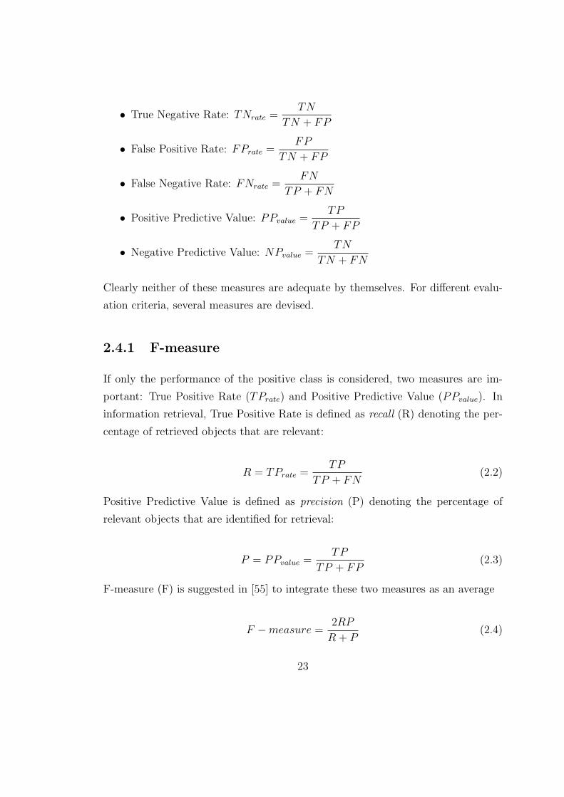
0 10
1
False Positive Rate
Tru
e P
ositi
ve R
ate
A
B
Figure 2.1: ROC curves for two different classifiers
(FPrate) on the X axis and the True Positive Rate (TPrate) on the Y axis, a Receiver
Operating Characteristics (ROC) graph plotted in Figure 2.1.
The ideal model is one that obtains 1 True Positive Rate and 0 False Positive
Rate (i.e., TPrate = 1 and FPrate = 0). Therefore, a good classification model
should be located as close as possible to the upper left corner of the diagram,
while a model that makes a random guess should reside along the main diagonal,
connecting the points (TPrate = 0, FPrate = 0), where every instance is predicted
as a negative class, and (TPrate = 1, FPrate = 1), where every instance is predicted
as a positive class. A ROC graph depicts relative trade-offs between benefits (true
positives) and costs (false positives) across a range of thresholds of a classification
model. A ROC curve gives a good summary of the performance of a classification
model. To compare several classification models by comparing ROC curves, it
is hard to claim a winner unless one curve clearly dominates the others over the
entire space [69]. The area under a ROC curve (AUC) provides a single measure
of a classifier’s performance for evaluating which model is better on average. It has
25

been shown that there is a clear similarity between AUC and well-known Wilcoxon
statistics [38].
26

Chapter 3
Ensemble Methods and AdaBoost
The use of ensemble methods has gained momentum in recent years [79, 94]. Re-
searchers have continuously explored the benefits of using ensemble methods to
solve complex recognition problems [48, 51]. An ensemble method for classifica-
tion tasks constructs a set of base classifiers from the training data and performs
classification by taking a vote on the prediction of each base classifier.
3.1 Classifier Ensemble Learning
The basic idea of classifier ensemble learning is to construct multiple classifiers from
the original data and then aggregate their predictions when classifying unknown
samples. There are a number of training parameters and factors which can be
manipulated to create ensemble members: the initial condition, the training data,
the architecture of the classifiers, and the training algorithm. The most frequently
used methods for creating ensembles are those which alter the training data, either
the training set or the input features [95]. Once a set of classifiers has been created,
an effective way of combining their outputs must be found [54]. A variety of schemes
have been proposed for combining multiple classifiers. The majority vote is by far
the most popular approach [94]. A general framework of the ensemble learning
27

�
�
��� �� �
��
���������
������������
�� �����
�� �� �������� �
����� ���
�� �����
��� ��������� �
�������� ���
�� �����
� � ��� ���
����������������������� ��
Figure 3.1: A General Framework of the Ensemble Learning Method
method by altering the training data is presented in Figure 3.1.
The main motivation for combining classifiers in redundant ensembles is to im-
prove their ability to generalization. Each component classifier is known to make
errors with the assumption that it has been trained on a limited set of data. How-
ever, the patterns that are misclassified by the different classifiers are not necessarily
the same [51]. This observation suggests that the use of multiple classifiers can en-
hance the recognition ability of the patterns under classification. Combining a set
of imperfect estimators is then viewed as a way to enhance the overall recognition
capability from the individual estimators with limitations.
The effect of combining redundant ensembles is also studied in terms of the
statistical concepts of bias and variance. Bias-variance decomposition is a formal
method for analyzing the prediction error of a predictive model. Given a classifier,
bias-variance decomposition distinguishes among: 1) the bias error, a systematic
component in the error associated with the learning method and the domain; 2) the
variance error, a component associated with differences in models between samples;
and 3) an intrinsic error, a component associated with the inherent uncertainty
in the domain [70]. The bias can be characterized as a measure of its ability to
generalize correctly to a test set, while the variance can be similarly characterized as
28

a measure of the extent to which the classifier’s prediction is sensitive to the data on
which it was trained. The variance is then associated with overfitting: if a method
overfits the data, the predictions for a single instance will vary between samples
[94]. There is a tradeoff between the bias and variance of training a classifier:
attempting to decrease the bias by considering more of the data will likely result
in a higher variance; trying to decrease the variance by paying less attention to the
data usually results in an increased bias. The improvement in performance arising
from ensemble combinations is usually the result of a reduction in variance, rather
than a reduction in bias. This occurs because the usual effect of ensemble averaging
is to reduce the variance of a set of classifiers, while leaving the bias unaltered.
3.2 Bagging
Bagging [8] is also known as bootstrap aggregating. Given a standard training set D
of size N , we generate L new training sets Di (i = 1 · ·L) also of size N by sampling
examples uniformly from D with replacements. By sampling with replacements it
is likely that some examples will be repeated in each Di. This kind of sample is
known as a bootstrap sample. The L models are fitted using the above L bootstrap
samples and are combined later in classification by voting.
Bagging improves the generalization error by reducing the variance of the base
classifiers. The performance of bagging depends on the stability of the base classi-
fier. If a base classifier is unstable (i.e., classifiers that undergo significant changes
in response to small perturbations of the training set or other training parameters),
bagging helps to reduce the variance errors. If a base classifier is stable, then the
error of the ensemble is primarily caused by bias in the base classifier. In this
case, bagging may not be able to improve the performance of the base classifier
significantly [85]. Hence, Bagging is believed to be effective especially for classifiers
characterized by a high variance and a low bias.
29

3.3 Random Forests
A random forest [10] is specially designed for decision tree classifiers. It combines
the predictions made by multiple decision trees, where each tree is generated based
on an independent set of random vectors of a data set. Let the number of training
samples be N and the number of variables be M . The number m (m << M) of
input variables is randomly selected to split at each node of the decision tree. The
tree is then grown to its entirety without any pruning. This may help reduce bias in
the resulting tree [85]. This procedure is repeated several times to construct several
classification trees. The predictions are then combined using a majority voting. To
increase randomness, bagging can also be used to generate bootstrap samples.
The strength and correlation of random forests may depend on the size of m. If
m is sufficiently small, then the tree tends to become less correlated. It is therefore
superior in handling a data set with a very large number of input variables. Since
only a subset of the features needs to be examined at each node, this approach helps
significantly to reduce the runtime of the algorithm. It has been shown empirically
that a random forest produces a highly accurate classifier [10].
3.4 Boosting
Boosting iteratively changes the data space and applies a base classification learning
algorithm to the updated data space so as to generate a sequence of classifiers.
Unlike bagging, boosting assigns a weight to each training sample and adaptively
changes the weight at each boosting round. Generally, boosting places greater
weights on those examples most often misclassified by the previous classifier so
that the next round of learning will focus on them. The weights assigned to the
training samples can be used in two ways: 1) they can be taken as probabilities of
samples to be selected; and 2) they can be used by the base classification learning
algorithm to model a classifier. Two fundamental questions of a boosting algorithm
are: 1) how to update the data space by altering the sample weights on each
30

boosting round; and 2) how to reduce several hypotheses to a single one. AdaBoost
[32] has addressed these two questions by selecting a special parameter α on each
round for both updating the data space and weighting the classifiers for voting.
By tuning such a parameter, AdaBoost holds many properties which become the
strong theoretic explanations for its success in producing accurate classifiers.
AdaBoost combines several classifiers. This suggests a major component in
variance reduction, like bagging. As stumps (single-split trees with only two termi-
nal nodes typically have low variance but high bias) are used as the base learner,
bagging performs very poorly and AdaBoost improves the base classification sig-
nificantly [33, 80]. This observation indicates that AdaBoost is also capable of bias
reduction.
3.4.1 AdaBoost Algorithm
AdaBoost for Bi-class Cases
The AdaBoost algorithm was originally designed for bi-class applications. The
algorithm takes as input a training set {(x1, y1), · · ·, (xM , yM)} where with the ith
sample (xi, yi): xi is an attribute value vector as a realization of the attribute set
X = {X1, X2, · · ·, XN}, and class label yi assumes a value in Y , with two classes,
assuming that Y = {−1, +1}. AdaBoost calls a given base learning algorithm
repeatedly in a series of rounds t = 1, · · ·, T . The weight of the ith training sample
on the iteration t is denoted by Dt(i). Initially, all weights are set equally. The
Pseudocode for AdaBoost is given in Figure 3.2.
The base learner’s task is to come up with a base classifier ht : X → Y based
on the distribution Dt to minimize the classification error. Once the base classifier
ht has been trained, AdaBoost chooses a parameter αt ∈ R which measures the
performance of the classification ht. The data distribution Dt is then updated. The
final classification criterion H is a weighted majority vote of the T base classifiers
where αt is the weight assigned to ht.
31

Given:{(x1, y1), · · ·, (xM , yM)} where xi ∈ X, yi ∈ Y = {−1, +1}Initialize D1(i) = 1/M .
For t = 1, · · ·, T :
1. Train the base learner ht: X → Y using distribution Dt
2. Calculate the error:
εt = Pri∼Di(ht(xi) 6= yi) (3.1)
3. Choose the weight updating parameter αt
4. Update and normalize sample weights:
Dt+1(i) =Dt(i)exp(−αtht(xi)yi)
Zt
(3.2)
Where, Zt is a normalization factor.
Output the final classifier:
H(x) = sign(T∑
t=1
αtht(x)) (3.3)
Figure 3.2: AdaBoost Algorithm
32

AdaBoost for Multi-class Cases
There are several methods of extending AdaBoost to the multi-class case. The
straightforward generalization approach, called AdaBoost.M1 in [32], is adequate
when the base learner is effective enough to achieve reasonably high accuracy (train-
ing error should be less than 0.5). See Figure 3.3 for its pseudocode.
This method fails if the learner cannot achieve at least 0.5 accuracy. In this
case, several more sophisticated methods have been developed [82]. These generally
work by reducing the multi-class problem to a larger binary class problem. However,
these methods require additional effort in the design of the base learning algorithm.
3.4.2 Choose Parameter α
With the AdaBoost algorithm for the bi-class cases, αt is specifically selected by
minimizing the training error of the combinational classifier. It has been shown in
[81] that the training error of the final classifier is bounded as
1
m|{i : H(xi) 6= yi}| ≤
∏t
Zt (3.8)
where
Zt =∑
i
Dt(i)exp(−αtyiht(xi)) (3.9)
=∑
i
Dt(i)(1 + yiht(xi)
2e−α +
1− yiht(xi)
2eα) (3.10)
Let
f(x) =T∑
t=1
αtht(x)
33

Given:{(x1, y1), · · ·, (xM , yM)} where xi ∈ X, yi ∈ Y = {c1, · · ·, ck}Initialize D1(i) = 1/M .
For t = 1, · · ·, T :
1. Train the base learner ht: X → Y using distribution Dt
2. Calculate the error: εt = Pri∼Di(ht(xi) 6= yi)
3. Choose the weight updating parameter αt
4. Update and normalize sample weights:
Dt+1(i) =Dt(i)exp(−αtI[ht(xi) = yi])
Zt
(3.4)
where Zt is a normalization factor, and
I[ht(xi) = yi] =
{+1 if ht(xi) = yi
−1 if ht(xi) 6= yi
(3.5)
Output the final classifier:
H(x) = arg maxci
(T∑
t=1
αt[ht(x) = ci]) (3.6)
Where for any predicate π,
[π] =
{1 if π holds
0 otherwise(3.7)
Figure 3.3: AdaBoost.M1 Algorithm
34

By unraveling the update rule of Equation 3.2, we have that
Dt+1(i) =exp(−∑
t αtht(xi)yi)
m∏
t Zt
=exp(−yif(xi))
m∏
t Zt
(3.11)
By the definition of the final hypothesis of Equation 3.3, if H(xi) 6= yi, then
yif(xi) ≤ 0 implying that exp(−yif(xi)) ≥ 1. Thus,
[H(xi) 6= yi] ≤ exp(−yif(xi)). (3.12)
Combining Equation 3.11 and 3.12 gives the error upper bound of Equation 3.8
since
1
m
∑i
[H(xi) 6= yi] ≤ 1
m
∑i
exp(−yif(xi)) (3.13)
=∑
i
(∏
t
Zt)Dt+1(i) =
∏t
Zt (3.14)
Let rt =∑
i
Dt(i)yiht(xi) in Equation 3.10, then minimizing Zt on each round,
αt is induced as
αt =1
2ln(
1 + rt
1− rt
) =1
2ln(
∑
i,yi=ht(xi)
Dt(i)
∑
i,yi 6=ht(xi)
Dt(i)) (3.15)
Plugging the value of αt into Equation 3.10, this gives the upper bound
Zt =√
1− r2t (3.16)
The training error of the composite classification H is at most∏
t
√1− r2
t . To min-
imize the overall training error, the learning objective on each round is to maximize
rt. Considering that
35

∑
i,yi 6=ht(xi)
Dt(i) =1− rt
2(3.17)
Maximizing rt is equivalent to minimizing the training error on each round.
The parameter α is specifically derived to minimize a training error upper bound
of the combinational classifier. With this setting of α, it is reasonable to model a
classifier that minimizes the training error on each round. Generally, given a classi-
fication learning algorithm, the learning objective is to minimize the training error.
By applying AdaBoost, it can be expected to achieve a combinational classifier with
its training error minimized.
In Section 6.2, we prove the bound (Equation 3.8) still holds on the training error
of the final hypothesis of AdaBoost.M1. By minimizing the error upper-bound, αt
of AdaBoost.M1 is induced in the same format as in Equation 3.15.
3.4.3 Weighting Efficiency
The sample weight updating goal of AdaBoost is to decrease the weight of training
samples which are correctly classified and increase the weights of those incorrectly
classified. Therefore, αt should be a positive value, demanding that the training
error should be less than randomly guessing (0.5) based on the current data distri-
bution; that is
∑
i,yi=ht(xi)
Dt(i) >∑
i,yi 6=ht(xi)
Dt(i) (3.18)
α is selected to minimize Z as a function of α (Equation 3.10). In the scenario
of the predictive attribute Y ∈ {−1, +1}, the first derivative of Z is
Z ′t(α) =
dZ
dα= −
∑i
Dt(i)ht(xi)yiexp(−αtht(xi)yi) (3.19)
= −Z∑
i
Dt+1(i)ht(xi)yi (3.20)
36
by definition of D(t+1) (Equation 3.2). To minimize Zt, αt is selected such that
Z ′(α) = 0
∑i
Dt+1(i)ht(xi)yi =∑
i,ht(xi)=yi
Dt+1(i)−∑
i,ht(xi)6=yi
Dt+1(i) = 0 (3.21)
That is
∑
i,ht(xi)=yi
Dt+1(i) =∑
i,ht(xi)6=yi
Dt+1(i) (3.22)
Hence, after weights have been updated, weight distributions on misclassified and
correctly classified samples are even. This makes the learning of the next iteration
to minimize∑
i,ht(xi)6=yi
Dt+1(i) the maximally difficult [81].
3.4.4 Forward Stagewise Additive Modelling
It has been shown that AdaBoost is equivalent to forward stagewise additive mod-
elling using an exponential loss function. The exponential loss function is related to
the Bernoulli likelihood [33]. From this point, the rather obscure work of the com-
putational learning is well explored in a likelihood method of standard statistical
practice [77]. The exponential loss function is defined as
L(y, f(x)) = exp(−yf(x)) (3.23)
where
f(x) =T∑
t=1
αtht(x) (3.24)
so that H(x) = sign(f(x)). Hence, on each round, one must solve
37

(αt, ht) = arg minα,h
∑i
exp[−yi(ft−1(xi) + αh(xi))] (3.25)
= arg minα,h
∑i
Dt(i)exp(−αyih(xi)) (3.26)
where, Dt(i) = exp(−yifm−1(xi)). The solution to Equation 3.26 is then obtained
in two steps. First, for any value of α > 0,
ht = arg minh
∑i
Dt(i)I[yi 6= ht(xi)] (3.27)
where, for any predicate π, I[π] equals 1 if π holds, 0 otherwise. Therefore, ht
is the classifier that minimizes the weighted error rate based on the current data
distribution. Once the classifier is fixed, the second step is to decide the value of α
to minimize the right side of Equation 3.26. This task is identical to the learning
objective of AdaBoost (Equation 3.10). Then α can be fixed as stated in Equation
3.15. The approximation is then updated as
ft(x) = ft−1(x) + αtht(x) (3.28)
which causes the weights for the next iteration to be
Dt+1(i) = Dt(i) · exp(−αtyiht(xi)) (3.29)
38

Chapter 4
Boosting An Associative Classifier
Experiments reported in [21, 56, 57, 61, 98, 104] show that associative classifica-
tion systems achieve competitive classification results with traditional classification
approaches such as C4.5. The reason is that the associative classifier is composed
of high quality rules, which are generated from highly confident event associations
that reflect the close dependencies among events. In addition, only significant rules
are employed when classifying a new object. Meanwhile, classification rules induced
from significant event associations are more easily understood by humans. Another
advantage of this approach is its greater flexibility in handling unstructured data.
Boosting is a popular method for improving the accuracy of any given learn-
ing algorithm. In the past several years, many publications have reported that
the AdaBoost algorithm has been successfully applied to most popular classifiers
[25, 31, 81, 83]. All of the reported works have shown impressive improvements
in the generalization behavior and the tendency of being robust against overfitting
in their experiments. To our knowledge, however, there is no reported work on
boosting associative classifiers. In this chapter, we attempt to apply the AdaBoost
algorithm to an associative classification system. Three types of associative classi-
fication systems are studied: 1) associative classifiers based on Apriori algorithm;
2) high-order pattern and weight-of-evidence rule-based classifier (HPWR); and 3)
associative classification by emerging patterns (EPs). In this research, we choose
39

HPWR classification system for apply the AdaBoost algorithm. In a more general
case, AdaBoost.M1 is implemented.
4.1 Association Mining
Association mining was first proposed to analyze basket data. The basket prob-
lem assumes that in a grocery shop there are a large number of items, such as
bread, milk, butter, beer, diapers and so on. Marketers would like to know what
items people often buy together. For example, it may be found through analyz-
ing transaction data that customers usually buy milk, butter and bread together.
Marketers can then use this information to place these items in proper locations
and adjust their selling strategies. In a similar manner, the same sort of ques-
tion is encountered in recommender systems, diagnosis decision support, intrusion
detection, etc. The challenge is how to discover those events that are frequently
associated together from large databases, especially when no domain knowledge is
available. Ever since its introduction, association mining has become an important
technique for knowledge discovery from databases (KDD). The Apriori algorithm
[2] is reported for the analysis of transactional data. This algorithm regards an
itemset, e.g., {milk, butter, bread}, as a frequent itemset if its frequency, which in-
dicates how often the component items occur together, is greater than a pre-defined
threshold. Each frequent itemset denotes one association pattern in a transactional
data set. Another well-developed method, which we refer to as high-order pattern
discovery [101], detects association patterns using residual analysis, which provides
a rigorous statistical base to justify the significance of the discovered patterns. In
their presentation, more general and formal terminologies are used: an item is de-
fined as a primary event, an itemset as a compound event and a frequent itemset
as an event association or association pattern. To present these two association
mining algorithms consistently, it is better to use the same terminology.
40

4.1.1 Terminology and Definitions
Consider a data set D containing M samples. Every sample x is described in terms
of N attributes, each of which can assume values in a corresponding discrete finite
alphabet. Let X = X1, X2, · · ·, XN represent this attribute set. Each attribute,
Xi, 1 ≤ i ≤ N , can be seen as a random variable taking on values from its alphabet
αi = α1i , · · ·, αmi
i , where mi is the cardinality of the alphabet of the ith attribute. An
additional attribute Y is considered as the target class with a set of k memberships
{c1, c2, ···, ck} denoting the set of k class members. A sample can then be represented
as {x, y}, where, x = {x1, · · ·, xN} is a realization of X, xi can assume any value in
αi and y can assume any value in Y . The jth sample in the database is denoted as
{xj, yj}, where 1 ≤ j ≤ M .
Definition 4.1.1 A primary event of a random variable Xi(1 ≤ i ≤ N) is a real-
ization of Xi, which takes on a value from αi.
We denote the pth(1 ≤ p ≤ mi) primary event of Xi as
[Xi = αpi ]
or simply xip. We use xi denoting a realization of Xi.
Let s be a subset of integers {1, · · ·, N} containing k elements (k ≤ N), and Xs
be a subset of X such that
Xs = {Xi|i ∈ s}
Then xsp denotes the pth realization of Xs. We use xs denoting a realization of Xs.
Definition 4.1.2 A compound event associated with the variable set Xs = {Xi|i ∈s} is a set of primary events instantiated by a realization xs. The order of the
compound event is |s|.
Definition 4.1.3 Let T be a statistical test. If a compound event xs passes the test
T, we say that the primary events of xs compose an event association, or xs is an
association pattern of order |s|.
41

4.1.2 Apriori Algorithm
Let us denote the frequency of observed occurrences of a compound event xs as oxs .
The support of the compound event xs is defined as its probability in the data set.
That is
support(xs) =oxs
M(4.1)
where M is the data size. A compound event xs can be considered as an association
pattern only if its support is greater than a pre-defined minimum support.
A general rule has the form of X ⇒ Y denoting that the observation of X
infers that Y is probably true. An association rule denotes the causal relationship
between two compound events. Let l and k be two subsets of integers {1, · · ·, N},where l ∩ k = φ. It follows then that X l and Xk are two subsets of X
X l = {Xi|i ∈ l}
and
Xk = {Xj|j ∈ k}
such that
X l⋂
Xk = φ
Let xl denote a realization of X l and xk a realization of Xk. To test if xl ⇒ xk is
an association rule, the measure confidence is defined as
confidence(xl ⇒ xk) =support(xk, xl)
support(xl)(4.2)
If the confidence(xl ⇒ xk) is greater than a pre-defined minimum confidence,
xl ⇒ xk can be considered as an association rule.
42

To detect all association patterns, the algorithm makes multiple passes over the
database. In the first pass, the algorithm simply counts primary event occurrences
to determine the 1-order compound event. In each subsequent pass, say pass k, the
algorithm starts with the (k-1)-order event associations found in the (k-1)th pass
and generates new possible compound events. Next, the database is scanned and
the supports of candidates are counted to determine which of the candidates are
association patterns. See [2] for more details.
4.1.3 High-Order Pattern Discovery Using Residual Analy-
sis
This method tests the statistical significance of the frequency of occurrences of a
pattern candidate against that of its expected number of occurrences [101]. The
expected number of occurrences of a compound event xs is its expected total num-
ber of occurrences under the assumption that the variables in Xs are mutually
independent. The expected number of occurrences of xs is denoted as
exs = M ·∏
i∈s,xi∈xs
P (xi) (4.3)
where P (xi) is estimated by the ratio of observed frequency of xi to the sample size
M .
To test whether or not xs is a significant association pattern, the standardized
residual, defined in [36], is used to scale the deviation between oxs and exs :
zxs =oxs − exs√
exs
(4.4)
The standardized residual zxs is the square root of chi-square χ2, having an
asymptotic normal distribution with a mean of approximately zero and a variance
of approximately one. Hence, if the absolute value of zxs exceeds 1.96, then, by
a conventional criteria, xs is considered as a significant association pattern with a
43

confidence level of 95%. The standardized residual is considered to be of normal
distribution only when the asymptotic variance of zxs is close to 1; otherwise, it has
to be adjusted by its variance for a more precise analysis. The adjusted residual is
expressed as
dxs =zxs√vxs
(4.5)
where vxs is the maximum likelihood estimate of the variance of zxs . More details
can be found in [101].
4.1.4 Computational Complexity
Association mining is time-consuming when data arrays contain a large number of
rows and/or columns. Many studies [2, 37, 101] indicate the inherent nature of a
combinatorially explosive number of event associations. Consider a data set with
N M-ary attributes. The total number of combinations of kth order association
patterns is given by
pk = (M)k ·(
N
k
), 2 ≤ k ≤ N (4.6)
where pk denotes the total number of primary event combinations at order k. There
are
(N
k
)sets of variables of size k and Mk possible events for each variable set.
The complexity of an algorithm which exhaustively searches high order patterns is
(M + 1)N . If the upper bound of the association order is set as K < N , the search
space isK∑
k=2
(Mk ·(
N
k
)).
Let the ratio of the number of pattern candidates of order k to the number of
candidates of order k − 1 be
ζk =pk
pk−1
=M · (N − k + 1)
k(4.7)
44

From the equation, we can observe that as the order of the patterns increases
from k=2 upwards, especially when k is small as compared to N, ζk increases rather
quickly. That is, the size of the search space for kth order patterns increases quickly
with respect to that of the (k − 1)th order patterns. For real world data, the
pattern associations are sparsely scattered rather than uniformly distributed in the
hypothesis space. If a compound event is not an association pattern of (k−1)-order,
it cannot be expanded as a higher order event association. All k-order association
pattern candidates are generated from (k − 1)-order association patterns. Thus,
the search complexity cannot be determined exactly since it is highly dependent
upon the characteristics of the input data. Some research efforts are reported to
deduce the computational complexity of association mining. Among them, the
algorithm FP-growth [37] mines association patterns without repeatedly scanning
the database, and checks a large set of candidates by pattern matching when using
the Apriori algorithm .
4.2 Associative Classifiers
4.2.1 Associative Classifiers Based on Apriori Algorithm
The Apriori algorithm finds all association rules in the database that satisfy the
pre-defined minimum support and minimum confidence constraints. For those as-
sociation rules detected, there is not a fixed target at the right-hand side. For
classification purposes, rules for prediction should have an identical pre-determined
target attribute. Works trying to induce classifiers from these discovered associa-
tion rules are reported in [57, 61, 96, 104]. Classification rules are extracted from
association rules by restricting the right-hand side to the classification attribute.
CBA [61] ranks these classification rules in sequence of their confidence, support
and the order of generation. A minimum set of classification rules are then cho-
sen according to the training error rate. In classifying an unknown case, the first
rule that satisfies the case will be used. If no rule applies, the default class (the
45

majority class) will be taken. CMAR [57] suggests a weighted χ2 analysis to per-
form a classification based on multiple association rules. Given a new data object,
CMAR collects the subset of rules matching the new object from the set of rules
for classification. These rules may not be consistent with the class labels. CMAR
first groups those according to class labels. Then, a ”combined effect” is accounted
for each group by adopting a weighted χ2 as the measure to determine the final
class membership of the object. Generally speaking, with the Apriori algorithm,
the setting of minimum support and confidence is rather ad hoc. The user typically
changes parameters and runs the mining algorithm many times in search of “op-
timal” results. Such a process is very time-consuming and little has been done to
alleviate it [17]. Meanwhile, how to measure the rule qualities when a large number
of rules are generated is another challenging issue.
4.2.2 Classification by Emerging Patterns
Emerging patterns (EPs) are defined as event associations whose supports change
significantly from one data set to another [20]. A data set is partitioned into several
subgroups according to their class labels. The difference in the supports of an event
association in one subgroup from those of an opposing group is measured. It is re-
ferred to as the growth rate. Those patterns whose growth rates satisfy a predefined
threshold are detected. They are regarded as capturing the class discriminant infor-
mation. Hence, such a pattern discovery process is directly classification-oriented.
Both CAEP [21] and DeEPs [56] employ EPs as classification rules. CAEP first
finds all the EPs from the training data of each class. When classifying a new
object by aggregating the differentiating power of the set of EPs that apply, a score
is obtained for each class, and that with the highest score wins. Arguing that the
process to discover all EPs from the training data is time-consuming, DeEPs pro-
pose a “lazy” learning approach. Whenever a new instance is being considered,
DeEPs uses it as a filter to remove irrelevant training values in order to reduce the
training space. Boundary EPs are detected for each class. To classify this instance,
a collective score for each class is calculated by summarizing the frequencies of the
46

selected EPs pertaining to each class. As an EP discovery process is instance-based,
all the training data should be stored for re-learning during the entire classification
process.
4.2.3 High-Order Pattern and Weight-of-Evidence Rule Based
Classifier
High-order pattern and weight of evidence rule-based classifier (HPWR) [97, 98] is a
well-developed classification system. As introduced in Section 4.1.3, the algorithm
of high-order pattern discovery detects significant association patterns by using
residual analysis in statistics. At the next stage, classification rules are generated
using weight of evidence to quantify the evidence of significant association patterns
in support of, or against, a certain class membership [98].
In information theory, the difference in the gain of mutual information when
predicting attribute Y takes on the value ci over that when it takes on some other
values, given x, is defined as the weight of evidence. This measure furnishes an
evidence provided by x in favor of ci being a plausible value of Y as opposed to
Y taking other values. Denoted by W (Y = ci/Y 6= ci|x), the weight of evidence
assumes the following forms
W (Y = ci/Y 6= ci|x) = I(Y = ci : x)− I(Y 6= ci : x) (4.8)
= logP (Y = ci|x)P (Y = ci)
− logP (Y 6= ci|x)P (Y 6= ci)
(4.9)
= logP (x|Y = ci)P (x|Y 6= ci)
(4.10)
where I(·) is the mutual information. The weight of evidence is positive if x provides
positive evidence supporting Y taking on ci; otherwise, it is negative, or zero.
As stated in [97, 98], significant event associations related to ci and x are used in
the classification inference process. Suppose that n sub-compound events x1, · · ·, xn
47

are detected, where (xk, Y = ci) is a significant association pattern and ∪nk=1xk = x;
xp
⋂xq = Φ when p 6= q, 1 ≤ k, p, q ≤ n. Then the weight of evidence W (Y =
ci/Y 6= ci|x) can be obtained from the sum of the weight of evidence provided by
each of them
W (Y = ci/Y 6= ci|x)
= logP (x1|Y = ci)
P (x1|Y 6= ci)+ ... + log
P (xn|Y = ci)
P (xn|Y 6= ci)(4.11)
= W (Y = ci/Y 6= ci|x1) + ... + W (Y = ci/Y 6= ci|xn) (4.12)
=n∑
k=1
W (Y = ci/Y 6= ci|xk) (4.13)
Thus, the calculation of weight of evidence is to find a proper set of disjoint signif-
icant event associations from x and to sum individual weight of evidence provided
by each of them. The task is to maximize the term in Equation 4.13. The most
plausible value ci of Y is the one that renders the highest weight.
4.2.4 Analysis
Among these three types of associative classification systems, certain similarities
and differences are present:
1. Associative classifiers based on the Apriori algorithm like CBA and HPWR
are typical associative classification systems. Traditionally, association and
classification are two independently important tasks for practical applications.
Association is mainly used in data mining for discovering descriptive knowl-
edge from databases, while classification is addressed in the field of machine
learning for exploring boundaries among classes. As association pattern min-
ing and classification rule mining are both indispensable in a data mining
system, there is a need to integrate both into an association classification
system. This is reflected by many research efforts to that effect. In general,
48

the pattern discovery phase detects all event associations without necessarily
relating the class it might be associated with. When the predicting attribute
for classification is given at the second stage, a subset of association patterns
or rules relevant to the predicting attribute is selected to construct a classifier.
Theoretically, when a different predicting attribute is assigned, no re-learning
is necessary for pattern discovery. Both CBA and HPWR share such a view.
On the other hand, the learning processes of CAEP and DeEPs are more like
those of a traditional classifier. Their classification rules are generated from
emerging patterns (EPs). The discovering of EPs is class-based (one class
against other classes) assuming the predicting attribute is known at the pat-
tern discovery phase. This learning process serves the purpose of classification
instead of exploring descriptive knowledge across the entire database.
2. HPWR, CAEP and DeEPs use multiple rules to classify a new object: HPWR
employs weight of evidence, which accounts for the strength of the association
between the class membership and all the admissible statistically significant
conditions. The total weights of evidence provided by several applicable pat-
terns are “addable” if they are conditionally independent [102]; CAEP obtains
a score for each class by aggregating the differentiating power of EPs which ap-
ply to the test object, and DeEPs determine collective scores for all classes by
compactly summarizing the number of occurrences of the discovered bound-
ary EPs. Thus, all relevant EPs of a class contribute to the final decision.
On the other hand, CBA uses only one rule for prediction. One problem with
this is that it cannot handle partial information from the test object [98]. For
example, if an unknown instance to be classified is O = [A,B,C] and accord-
ing to rule1: A ⇒ class1, O belongs to class1, but according to rule2: B ⇒class2 and rule3: C ⇒ class2, O belongs to class2. Then CBA will classify O
as class1 since rule1 precedes rule2 and rule3 even though the combination of
rule2 and rule3 might be more determining.
3. HPWR discovers all the association patterns using residual analysis. The sta-
tistical significance of an association pattern is guaranteed, which eliminates
49

the need of using unstandardized (widely varying) and arbitrary thresholds.
Meanwhile, the residual is easily interpreted in terms of the degree of sat-
isfaction in the discovery when compared with others. CBA employs the
Aproiri algorithm to detect association rules by testing their supports and
confidences. EPs used by CAEP and DeEPs are discovered by calculating
their supports in one class against others and obtaining a growth rate re-
flecting the significance of the support changes. One learning issue with the
latter two pattern discovery methods, the Aproiri algorithm and EPs mining,
is the setting of the threshold: with the Apriori algorithm, it is the minimum
support and minimum confidence; with EP mining, it is the growth rate (set
as infinite in DeEPs).
4.3 Boosting the HPWR Classification System
There are two approaches in applying the AdaBoost.M1 (Figure 3.3) algorithm to
a specific base learner. One is to resample instances from the original data set.
The probabilities of samples to be selected are not equal across the entire training
set. They depend on how often these samples were misclassified by the previous
classifiers. Normalized sample weights become the new probability values of the
samples to be selected. The other approach is to introduce sample weights into the
learning process directly. Some evidence indicates that the latter works better in
practice due to less information loss [73, 83].
Sample weights can be induced into the learning process directly when boosting
an HPWR classification system. The learning process of HPWR tests the occur-
rences or probabilities of event associations in the samples. A normalized sample
weight can be taken as the occurrence probability of the sample. The observed
probability of an event or an event association can then be calculated as the sum-
mation of weights of samples in which this event or event association occurs.
50

4.3.1 Residual Analysis on Weighted Samples
Let D(i) denote the weight of the ith sample. After normalization over all the
database, each weight can be taken as the probability of the sample, as well as the
probability of each primary event in this sample. Thus, the relative frequency of
occurrences, of a primary event of xi can be calculated as
oxi= M · P (xi) = M ·
M∑j=1,xi∈xj
D(j) (4.14)
The observed number of occurrences of compound event xs as oxs and its ex-
pected number of occurrences as
oxs = M · P (xs) = M ·M∑
j=1,xs∈xj
D(j) (4.15)
exs = M ·∏
xi∈xs
p(xi) = M ·∏
xi∈xs
M∑j=1,xi∈xj
D(j) (4.16)
To determine whether a compound event xs is a pattern or not, the Standardized
Residual (Equation 4.4) or Adjusted Residual (Equation 4.5) is tested.
4.3.2 Weight of Evidence Provided by Weighted Samples
Suppose there are n sub-compound events x1, ···, xn are detected, where (xk, Y = cj)
is a significant association pattern and ∪nk=1xk = x; xp
⋂xq = Φ when p 6= q,
1 ≤ k, p, q ≤ n. Then
P (xk, Y = cj) =M∑
i=1,xk∈xi,yi=cj
D(i) (4.17)
51

P (Y = cj) =M∑
i=1,yi=cj
D(i) (4.18)
and,
P (xk|Y = cj) =P (xk, Y = cj)
P (Y = cj)(4.19)
In the like manner, we have
P (xk, Y 6= cj) =M∑
i=1,xk∈xi,yi 6=cj
D(i) (4.20)
P (Y 6= cj) =M∑
i=1,yi 6=cj
D(i) (4.21)
and
P (xk|Y 6= cj) =P (xk, Y 6= cj)
P (Y 6= cj)(4.22)
The weight of evidence W (Y = ci/Y 6= ci|xk) provided by xk in support of, or
against, cj can then be obtained from Equation 4.19 and Equation 4.22 as
w(Y = cj/Y 6= cj|xk) = logP (xk|Y = cj)
P (xk|Y 6= cj)(4.23)
The sum of the weight of evidence provided by each of xk (1 ≤ k ≤ n) are then
obtained by Equation 4.13.
4.3.3 Weighting Strategies for Voting
We assume that a new observation, x, is to be classified into one of the class labels
in Y= {c1, c2, · · ·, ck}. The most plausible value of Y is the one with the highest
52

weight of evidence provided by the observation. The weight of evidence provided
by x in favor of ci as opposed to other values is expressed as ri:
ri = W (Y = ci/Y 6= ci|x) = logP (x|Y = ci)
P (x|Y 6= ci)(4.24)
Therefore, the output of the tth classifier ht learned through HPWR can be pre-
sented in the following two ways:
ht(x) → ci, 1 ≤ i ≤ k (4.25)
or
h′t(x) → ci, with confidence rti 1 ≤ i ≤ k (4.26)
In Equation 4.25, only the class label assignment is considered, while in Equation
4.26 both the class label assignment and the confidence level evaluated by the
weight of evidence are considered. When voting multiple classifiers by applying the
AdaBoost.M1 algorithm, these two versions of component classifier outputs can be
plugged into Equation 3.6 to get the combination classification. Based on these
two versions of outputs, we explore three weighting strategies for voting the final
hypothesis:
•Strategy 1 (Classifier-based weighting strategy). If we only consider
the class label assignment of each classifier while ignoring the weight of evidence
in HPWR (i.e., Equation 4.25), Equation 3.6 remains the same. This is exactly
the voting strategy used in the AdaBoost.M1 algorithm. Voting factor α is deter-
mined by the classifier’s performance based on training error. A certain component
classifier will provide the same confidence in classifying a set of objects via voting.
Therefore, we call this strategy classifier-based weighting.
•Strategy 2 (Sample-based weighting strategy). Noticing that both the
classifier weighting factor, α, in AdaBoost.M1 and the weight of evidence, r, in
HPWR are strength measures in deciding a class label, we replace α with r in
53

Equation 3.6. The weighted combination of the output of each classifier then be-
comes:
H(x) = arg maxci,i=1··k
(T∑
t=1
rtiI[ht(x) = ci]) (4.27)
This weighting strategy uses the weight of evidence of each classifier in support-
ing or rejecting a class label given a new object as the confidence measure for voting
the final classification. As each classifier provides a specific prediction confidence
for each sample, this weighting scheme is called sample-based weighting.
•Strategy 3 (Hybrid weighting strategy). In this strategy, we consider
both the class label assignment and the prediction confidences evaluated in terms
of the weight of evidence as the outputs of a classifier. That is, we apply both h′t(x)
and rti in Equation 4.26 to Equation 3.6. The weighted combination of the output
of each classifier then becomes:
H(x) = arg maxci,i=1··k
(T∑
t=1
αtrtiI[ht(x) = ci]) (4.28)
Here, the weight of a classifier in voting is a product of the classifier weighting
factor, α, in AdaBoost.M1 and the weight of evidence, r, of HPWR. We call this
strategy Hybrid weighting.
The weighting strategy of the original AdaBoost.M1 algorithm is classifier-based
(Strategy 1). The intention of a boosting algorithm is to force each learning iteration
to concentrate on a specific part of the data space by changing the data distribution.
It is quite possible that a classifier has different prediction confidences in different
data spaces. When a classifier-based weighting scheme is adopted, this difference
is overlooked in voting. Sample-based weighting strategy (Strategy 2) uses rti, the
weight of evidence rendered for each test object as the voting factor in the final
classification. The obvious advantage of a sample-based weighting scheme is that
it takes into account the different voting priorities with respect to each classifier’s
54

learning space. The hybrid strategy (Strategy 3) is a combination of Classifier-
based and Sample-based weighting strategies, where the voting weight of a classifier
is calculated as a product of the weight of evidence, rti, of the classification inference
in HPWR by the classifier weighting factor, α, in the AdaBoost.M1 algorithm.
55

Chapter 5
Boosting for Learning Bi-Class
Imbalanced Data
5.1 Why Boosting?
The performance of a range of well-developed classification systems is degraded
when encountering the class imbalance problem. The major research objective of
this thesis is to investigate a solution which is applicable to most classifier learn-
ing algorithms to enhance the classification of imbalanced data. Solutions at the
algorithm-level change the underlying learning methods, and so are unique to spe-
cific classification systems. Since the most obvious characteristic of an imbalanced
data set is the skewed data distributions among classes, the straightforward solu-
tions at the data-level is to manually generate a balanced data set by resampling.
These solutions are applicable to most classification systems without changing their
learning methods. However, as stated in Section 2.3.1, the significant shortcomings
with the resampling approach are:
1. The optimal class distribution is always unknown;
2. The criterion in selecting samples is uncertain;
56
3. Undersampling the prevalent class may risk information loss; and
4. Oversampling the small class may risk model overfitting.
Ensemble methods, such as boosting and bagging, construct multiple classifiers
by resampling the data space: weighting samples by boosting and replacing samples
by bagging. The improvement in performance arising from ensemble combinations
is usually the result of a reduction in variance. Variance measures how much a
learning algorithm’s guess bounces around for different training sets. Variance is
therefore associated with overfitting: if a method overfits the data the predictions
for a single instance will vary between samples. Both boosting and bagging are
capable of reducing variance, and hence are immune to the model overfitting prob-
lem.
According to the bias-variance decomposition analysis, the model bias also con-
tributes to the prediction error of a classifier. With an imbalanced data set, small
class samples occurring infrequently, models that describe the rare classes have to
be highly specialized. Standard learning methods pay less attention to the rare
samples as they try to extract the regularities from the data set. Such a model
performs poorly on the rare class due to the introduced bias error. Bagging is be-
lieved to be effective for variance reduction, but not for bias reduction. AdaBoost,
however, is stated to be capable of both bias and variance reduction [33].
The AdaBoost algorithm weighs each sample to reflect its importance and places
the greatest weights on those samples which are most often misclassified by the
preceding classifiers. The sample weighting strategy is equivalent to re-sampling
the data space combining both up-sampling and down-sampling. Boosting attempts
to reduce the bias error as it focuses on misclassified samples [31]. Such a focus
may cause the learner to produce an ensemble function that differs significantly
from the single learning algorithm. Hence the advantages of AdaBoost for learning
imbalanced data can be summarized as:
1. A boosting algorithm is applicable to most classification systems;
57

2. Resampling the data space automatically eliminates the extra learning cost
for exploring the optimal class distribution and the representative samples;
3. Resampling the data space through weighting each sample results in little
information loss as compared with eliminating some samples from the data
set;
4. Combining multiple classifications decreases the risk of model overfitting; and
5. AdaBoost is capable of reducing the bias error of a certain classification learn-
ing method.
These positive features make the boosting approach an attractive technique
in tackling the class imbalance problem. Given a data set with an imbalanced
class distribution, misclassified samples are often in the minority class. When the
AdaBoost algorithm is applied, samples in the minority class may receive more
weights such that successive learning will focus on the minority class. Intuitively,
the AdaBoost algorithm might improve the classification performance on the small
class. However, experimental results reported in [29, 47, 88] show that the im-
proved identification performances for the small class are not always guaranteed or
satisfactory. The straightforward reason is that AdaBoost is accuracy-oriented: its
weighting strategy may bias towards the prevalent class since it contributes more
to the overall classification accuracy. Hence, the issue becomes how to adapt the
AdaBoost algorithm to incline its boosting strategy towards the class of interest.
5.2 Cost-Sensitive Boosting Algorithms
The weighting strategy of AdaBoost is to increase weights of misclassified samples
and decrease weights of correctly classified samples until the weighted sample dis-
tributions between misclassified samples and correctly classified samples are even
on each round. This weighting strategy distinguishes samples on their classification
58

outputs: correctly classified or misclassified. However, it treats samples of differ-
ent types (classes) equally: weights of misclassified samples from different classes
are increased by an identical ratio, and weights of correctly classified samples from
different classes are decreased by another identical ratio. Given a bi-class data
set with imbalanced class distributions, samples of the rare class are prone to be
misclassified. Due to the relatively few samples in the rare class, the number of
misclassified samples in the rare class is smaller than that of the prevalent class.
For example, consider a data set with class distributions of 10% of the rare class
and 90% of the prevalent class. Suppose that after a classification process, the
average classification error rate is 20%, with 60% of the rare samples and 15.6%
of the prevalent samples misclassified. By weight updating of AdaBoost, on the
next round the weighted sample distributions will be 17.5% of the rare class and
82.5% of the prevalent class. Even though the class distribution of the rare class
is improved, it is still smaller than that of the prevalent class. The learning objec-
tive in dealing with the imbalanced class problem is to improve the identification
performance for the small class. This learning objective expects that the weighting
strategy of a boosting algorithm will preserve a considerable weighted sample size
of the small class. A desirable boosting strategy is one which is able to distinguish
samples from different classes, and boost more weights on those samples associated
with higher identification importance.
To denote the different identification importance among samples, each sample
is associated with a cost item: the higher the value, the greater the importance of
correctly identifying that sample. Let {(x1, y1, C1), · · ·, (xm, ym, Cm)} be a sequence
of training samples, where each xi is an n-tuple of attribute values; yi is a class
label in Y = {−1, +1}; and Ci ⊂ [0, +∞) is an associated cost item. For an
imbalanced data set, samples with class label y = −1 are much more than samples
with class label y = +1. As the learning objective is to improve the identification
performance for the small class, the cost values associated with samples of the
small class can be set higher than those associated with samples of the prevalent
class. Keeping the same learning framework of AdaBoost, the cost items can be fed
59
into the weight updating formula of AdaBoost (Equation 3.2) to bias its weighting
strategy. There are three ways to introduce cost items into the weight updating
formula of AdaBoost: inside the exponent, outside the exponent, and both inside
and outside the exponent. Three modifications of Equation 3.2 then become:
• Modification I
Dt+1(i) =Dt(i)exp(−αtCiht(xi)yi)
Zt
(5.1)
• Modification II
Dt+1(i) =Ci ·Dt(i)exp(−αtht(xi)yi)
Zt
(5.2)
• Modification III
Dt+1(i) =Ci ·Dt(i)exp(−αtCiht(xi)yi)
Zt
(5.3)
Each modification can be taken as a new boosting algorithm denoted as AdaC1,
AdaC2 and AdaC3, respectively. As these algorithms use cost items, they can also
be regarded as cost-sensitive boosting algorithms. For the AdaBoost algorithm,
the selection of the weight updating parameter is crucial in converting a weak
learning algorithm into a strong one [33]. When the cost items are introduced
into the weight updating formula of the AdaBoost algorithm, the updated data
distribution is affected by the cost items. Without re-inducing the weight updating
parameter taking the cost items into consideration for each cost-sensitive boosting
algorithm, the boosting efficiency is not guaranteed. With the AdaBoost algorithm,
the weight updating parameter α is calculated to minimize the overall training error
of the combined classifier. Using the same inference method, we induce the weight
updating parameter α for each algorithm.
5.2.1 AdaC1
Unravelling the weight updating rule of Equation 5.1, we obtain
60

Dt+1(i) =exp(−∑
t αtCiyiht(xi))
m∏
t Zt
=exp(−Ciyif(xi))
m∏
t Zt
(5.4)
where
Zt =∑
i
Dt(i)exp(−αtCiyiht(xi)) (5.5)
and
f(xi) =∑
t
αtht(xi) (5.6)
The over all training error is bounded as
1
m|{i : H(xi) 6= yi}| ≤ 1
m
∑i
exp(−Ciyif(xi)) (5.7)
=∑
i
(∏
t
Zt)Dt+1(i) =
∏t
Zt (5.8)
Thus, the learning objective on each boosting iteration is to find αt so as to minimize
Zt (Equation 5.5). According to [81], once Ciyiht(xi) ∈ [−1 + 1], the following
inequality holds
∑i
Dt(i)exp(−αCiyih(xi)) ≤∑
i
Dt(i)(1 + Ciyiht(xi)
2e−α +
1− Ciyiht(xi)
2eα)
(5.9)
By zeroing the first derivative of the right hand side of the Inequality 5.9, αt can
be determined as
αt =1
2log
1 +∑
i,yi=ht(xi)
Ci ·Dt(i)−∑
i,yi 6=ht(xi)
Ci ·Dt(i)
1−∑
i,yi=ht(xi)
Ci ·Dt(i) +∑
i,yi 6=ht(xi)
Ci ·Dt(i)(5.10)
61

To ensure that the selected value of αt is positive, the following condition should
hold
∑
i,yi=ht(xi)
Ci ·Dt(i) >∑
i,yi 6=ht(xi)
Ci ·Dt(i) (5.11)
The Pseudocode for AdaC1 is given in Figure 5.1.
Let rt =∑
i
Dt(i)Ciyiht(xi), then αt =1
2log
1 + rt
1− rt
. By plugging αt into Equa-
tion 5.9, it can be proved by the method used in [81] that the training error of the
composite classification H is at most∏
t
√1− r2
t . To minimize the overall training
error, the learning objective on each round is to maximize rt. Considering that
rt =∑
i,yi=ht(xi)
Ci ·Dt(i)−∑
i,yi 6=ht(xi)
Ci ·Dt(i) (5.12)
maximizing rt is equivalent to minimizing the cost error∑
i,yi 6=ht(xi)
Ci ·Dt(i) on each
round. This observation is based on the fact that αt is approximated by minimizing
an upper bound of the Zt. In the upper bound (Equation 5.9), each sample is
weighted by its cost item. It turns out that to minimize the upper bound, a classifier
should minimize the cost error.
5.2.2 AdaC2
Unravelling the weight updating rule of Equation 5.2, we obtain
Dt+1(i) =Ct
iexp(−∑t αtyiht(xi))
m∏
t Zt
=Ct
iexp(−yif(xi))
m∏
t Zt
(5.13)
where f(xi) is the same as defined in Equation 5.6 and
Zt =∑
i
Ci ·Dt(i)exp(−αtyiht(xi)) (5.14)
62

Given:{(x1, y1, C1), · · ·, (xM , yM , CM)} where xi ∈ X, yi ∈ Y = {−1, +1},Ci ∈ (0 + 1], i = 1 · ·MInitialize D1(i) = 1/M .
For t = 1, · · ·, T :
1. Train the base learner ht: X → Y using distribution Dt
2. Choose the weight updating parameter:
αt =1
2log
1 +∑
i,yi=ht(xi)
Ci ·Dt(i)−∑
i,yi 6=ht(xi)
Ci ·Dt(i)
1−∑
i,yi=ht(xi)
Ci ·Dt(i) +∑
i,yi 6=ht(xi)
Ci ·Dt(i)
3. Update and normalize the sample weights:
Dt+1(i) =Dt(i)exp(−αtCiht(xi)yi)
Zt
Where, Zt is a normalization factor:
Zt =∑
i
Dt(i)exp(−αtCiyiht(xi))
Output the final classifier:
H(x) = sign(T∑
t=1
αtht(x))
Figure 5.1: AdaC1 Algorithm
63

Then, the training error of the final classifier is bounded as
1
m|{i : H(xi) 6= yi}| ≤ 1
m
∑i
exp(−yif(xi)) =∏
t
Zt
∑i
CiDt(i)
C(t+1)i
(5.15)
Where C(t+1)i denotes the (t+1)th power of Ci. There exists a constant γ such that
∀i, γ < C(t+1)i . Then,
1
m|{i : H(xi) 6= yi}| ≤
∏t
Zt
∑i
Ci ·Dt(i)
C(t+1)i
≤ 1
γ
∏t
Zt (5.16)
Since γ is a constant, the learning objective at each boosting iteration is to find αt
so as to minimize Zt (Equation 5.14). Zt can be expressed as
∑i
Ci ·D(i)(t)exp(−αyiht(xi)) =∑
i
Ci ·Dt(i)(1 + yiht(xi)
2e−α +
1− yiht(xi)
2eα)
(5.17)
Zeroing the first derivative of the right hand side, αt is then uniquely selected as
αt =1
2log
∑
i,yi=ht(xi)
Ci ·Dt(i)
∑
i,yi 6=ht(xi)
Ci ·Dt(i)(5.18)
To ensure that the selected value of αt is positive, the following condition should
hold
∑
i,yi=ht(xi)
Ci ·Dt(i) >∑
i,yi 6=ht(xi)
Ci ·Dt(i) (5.19)
The Pseudocode for AdaC2 is given in Figure 5.2.
64

Given:{(x1, y1, C1), · · ·, (xM , yM , CM)} where xi ∈ X, yi ∈ Y = {−1, +1},Ci ⊂ (0, +∞), i = 1 · ·MInitialize D1(i) = 1/M .
For t = 1, · · ·, T :
1. Train the base learner ht: X → Y using distribution Dt
2. Choose the weight updating parameter:
αt =1
2log
∑
i,yi=ht(xi)
Ci ·Dt(i)
∑
i,yi 6=ht(xi)
Ci ·Dt(i)
3. Update and normalize the sample weights:
Dt+1(i) =Ci ·Dt(i)exp(−αtht(xi)yi)
Zt
Where, Zt is a normalization factor:
Zt =∑
i
Ci ·Dt(i)exp(−αtyiht(xi))
Output the final classifier:
H(x) = sign(T∑
t=1
αtht(x))
Figure 5.2: AdaC2 Algorithm
65

Let rt =∑
i
CiDt(i)yiht(xi) and Rt =
∑i
CiDt(i), then αt =
1
2log
Rt + rt
Rt − rt
. Plug-
ging into Equation 5.17, we can derive that
Zt =√
R2t − r2
t (5.20)
The training error of the composite classification H is at the most1
γ
T∏t=1
√R2
t − r2t .
With Rt and γ as constants, to minimize the overall training error, learning objec-
tive on each round is to maximize rt. Considering that
rt =∑
i,yi=ht(xi)
CiDt(i)−
∑
i,yi 6=ht(xi)
Ci ·Dt(i) (5.21)
maximizing rt is equivalent to minimizing the cost error∑
i,yi 6=ht(xi)
Ci ·Dt(i) on each
round. Since the cost item is used to weigh each sample directly, it is understandable
that the learning objective is to minimize the cost error on each round.
5.2.3 AdaC3
The weight updating formula (Equation 5.3) of AdaC3 is a combination of AdaC1
and AdaC2 (with the cost items being both inside and outside the exponential
function). The training error bound of AdaC3 can then be expressed as
1
m|{i : H(xi) 6= yi}| ≤ 1
γ
∏t
Zt (5.22)
where γ is a constant and ∀i, γ < C(t+1)i , and
Zt =∑
i
Ci ·Dt(i)exp(−αtCiyiht(xi)) (5.23)
66

Since γ is a constant, the learning objective at each boosting iteration is to find αt
so as to minimize Zt (Equation 5.23). According to [81], once Ciyiht(xi) ∈ [−1, +1],
the following inequality holds
∑i
Ci ·Dt(i)exp(−αCiyih(xi)) ≤∑
i
Ci ·Dt(i)(1 + Ciyiht(xi)
2e−α +
1− Ciyiht(xi)
2eα)
(5.24)
By zeroing the first derivative of the right hand side of Inequality 5.24
αt =1
2log
∑i
Ci ·Dt(i) +∑
i,yi=ht(xi)
C2i D
t(i)−∑
i,yi 6=ht(xi)
C2i D
t(i)
∑i
Ci ·Dt(i)−∑
i,yi=ht(xi)
C2i D
t(i) +∑
i,yi 6=ht(xi)
C2i D
t(i)(5.25)
To ensure that the selected value of αt is positive, the following condition should
hold:
∑
i,yi=ht(xi)
C2i D
t(i) >∑
i,yi 6=ht(xi)
C2i D
t(i) (5.26)
The Pseudo code for AdaC3 is given in Figure 5.3.
Let rt =∑
i
C2i ·Dt(i)yiht(xi) and Rt =
∑i Ci · Dt(i), then αt =
1
2log
Rt + rt
Rt − rt
.
Plugging into Equation 5.24, we can derive the upper bound of Zt
Zt ≤√
R2t − r2
t (5.27)
The training error of the composite classification H is at the most1
γ
T∏t=1
√R2
t − r2t .
With Rt and γ as constants to minimize the overall training error, the learning
objective on each round is to maximize rt. Considering that
67

Given:{(x1, y1, C1), · · ·, (xM , yM , CM)} where xi ∈ X, yi ∈ Y = {−1, +1},Ci ∈ (0 + 1], i = 1 · ·MInitialize D1(i) = 1/M .
For t = 1, · · ·, T :
1. Train the base learner ht: X → Y using distribution Dt
2. Choose the weight updating parameter:
αt =1
2log
∑i
Ci ·Dt(i) +∑
i,yi=ht(xi)
C2i D
t(i)−∑
i,yi 6=ht(xi)
C2i D
t(i)
∑i
Ci ·Dt(i)−∑
i,yi=ht(xi)
C2i D
t(i) +∑
i,yi 6=ht(xi)
C2i D
t(i)
3. Update and normalize the sample weights:
Dt+1(i) =Ci ·Dt(i)exp(−αtCiht(xi)yi)
Zt
Where, Zt is a normalization factor:
Zt =∑
i
Ci ·Dt(i)exp(−αtCiyiht(xi))
Output the final classifier:
H(x) = sign(T∑
t=1
αtht(x))
Figure 5.3: AdaC3 Algorithm
68

rt =∑
i,yi=ht(xi)
C2i D
t(i)−∑
i,yi 6=ht(xi)
C2i D
t(i) (5.28)
maximizing rt is equivalent to minimizing∑
i,yi 6=ht(xi)
C2i ·Dt(i) (i.e., training error
weighted by the square of the cost item) on each round. The weighting strategy of
AdaC3 is a combination of AdaC1 and AdaC2. αt is approximated by minimizing
an upper bound of the Zt (Equation 5.24), where each sample is weighted by its
cost item twice. It turns out that to minimize the upper bound, a classifier should
minimize the cost error weighted by the square of the cost item.
5.2.4 Analysis
By introducing the cost item into the weight updating formula of AdaBoost in
different ways, three cost-sensitive boosting algorithms, namely AdaC1, AdaC2 and
AdaC3, are developed. It is easy to prove that if each individual cost item is set as
1 (i.e., Ci = 1), the proposed three cost-sensitive AdaBoost algorithms will reduce
to the original AdaBoost algorithm. The main step of each cost-sensitive boosting
algorithm is the inference of the weight updating parameter for each algorithm
taking the cost item into consideration. This parameter is used for updating sample
weights and voting a set of classifiers as well.
Let αC1, αC2, and αC3 denote the weight updating parameters of AdaC1, AdaC2
and AdaC3, respectively. Using the same inference method by AdaBoost, each of
them is reduced by minimizing its sample weight normalization factor Zt. αC1 and
αC3 are approximated by minimizing the upper bounds of Zt respectively, and αC2
is an exact solution to minimize its Zt. By the solutions of α, the learning objectives
for AdaC1 and AdaC2 are to minimize the cost error∑
i,yi 6=ht(xi)
Ci ·Dt(i) and that
of AdaC3 is to minimize the squared-cost error∑
i,yi 6=ht(xi)
C2i ·Dt(i) on each round.
The goal to develop the cost-sensitive boosting algorithms is to improve the
69
standard classification learning algorithms’ identification performances on the im-
portant class. Generally, the learning objective of a standard classification learning
algorithm is to minimize the error instead of the cost error. However, if each sam-
ple is associated with a cost item, the learning objective of minimizing the training
error can be transferred to minimizing the cost error by applying the Translation
Theorem (Equation 2.1). That is, in weighting each sample by its associated cost
item, the classifier which optimizes error rate will optimize the cost error on the
updated data space [106].
AdaC2 weighs each sample by its associated cost item according to the definition
of Dt+1 of Equation 5.2. Thus, by applying the AdaC2 algorithm, a classifier that
minimizes the error rate will minimize the cost error simultaneously. On each round,
the first derivative of Zt (Equation 5.14) as a function of αt (αC2) is
Z ′t(α) =
dZt
dαt
= −∑
i
Ci ·Dt(i)ht(xi)yiexp(−αtyiht(xi)) = 0 (5.29)
By the weight updating formula of AdaC2 (Equation 5.2), the unique solution for
αt (αC2) makes
∑
i,ht(xi)=yi
Dt+1(i) =∑
i,ht(xi)6=yi
Dt+1(i) (5.30)
That is, weight distributions on the correctly classified samples and misclassified
samples are even. Similar to AdaBoost, this makes the learning of the next iteration
to minimize the training error maximally difficult.
The weighting strategy of AdaC1 does not update sample weights by the cost
items. By applying AdaC1, a standard learning algorithm can not minimize the
cost error on each round as expected. AdaC3 weighs each sample by the cost item
once. By applying AdaC3, a standard learning algorithm is able to minimize the
cost error. Expected by the AdaC3 algorithm, however, the learning objective
should be to minimize the squared-cost error.
70

5.3 Cost-Sensitive Exponential Loss and AdaC2
AdaC2 tallies with the stagewise additive modelling, where steepest descent search
is carried on to minimize the overall cost loss under the exponential function. By
integrating a cost item C into Equation 3.23, the cost-sensitive exponential loss
function becomes
C · L(y, f(x)) = C · exp(−yf(x)) (5.31)
The goal is to train a classifier which minimizes the expected cost loss under the
exponential function. On each iteration, ht and αt is learned separately to solve
(αt, ht) = arg minα,h
∑i
Ci · exp[−yi(ft−1(xi) + αh(xi))] (5.32)
= arg minα,h
∑i
Ci ·Dt(i)exp(−αyih(xi)) (5.33)
where Dt(i) = exp(−yifm−1(xi)). The solution to Equation 5.33 is obtained in two
steps. First, for any value of α > 0, ht is the one which minimizes the cost error,
which is
ht = arg minh
∑i
Ci ·Dt(i)I[yi 6= ht(xi)] (5.34)
Standard classification learning algorithms minimize the error rate instead of the
expected cost. However, the translation theorem derived in [106] can be applied
to solve this problem. Against a normal space without considering the cost item,
a data space associated with different cost factors is regarded as a cost-space. If
we have examples drawn from a distribution in the cost-space, then we can have
another distribution in the normal space. In our case, weighing each sample by its
cost item, we obtain a sample distribution in the normal space
71

Dt(i) = Ci ·Dt(i) (5.35)
According to the translation theorem, those optimal error rate classifiers for
D will be optimal cost minimizers for D. Thus, ht can be fixed to minimize the
error rate for Dt, which is equivalent to minimizing the cost error for Dt. Once the
classifier is fixed, the second step is to decide the value of α to minimize the right
side of Equation 5.33. This job shares the learning objective of AdaC2 (Equation
5.14). α is fixed as stated in Equation 5.18. The approximation is then updated as
ft(x) = ft−1(x) + αtht(x) (5.36)
which causes the weights for the next iteration to be
Dt+1(i) = Dt(i) · exp(−αtyiht(xi)) (5.37)
To minimize the cost-sensitive exponential loss (Equation 5.31), the learning objec-
tive on each round is to minimize the expected cost. By applying the translation
theorem, each sample is reweighted by its cost factor. Therefore, each sample weight
for learning of the next iteration is updated as
Dt+1(i) = Ci ·Dt(i) · exp(−αtyiht(xi)) (5.38)
5.4 Cost Factors
For cost-sensitive boosting algorithms, the cost items are used to characterize the
identification importance of different samples. The cost value of a sample may
depend on the nature of the particular case [91]. For example, in detection of
fraud, the cost of missing a particular case of fraud will depend on the amount
of money involved in that particular case [30]. Similarly, the cost of a certain
72

kind of mistaken medical diagnosis may be conditional on the particular patient
who is misdiagnosed [91]. In the case that the misclassification costs or learning
importance for samples in one class are the same, a unique number can be set up
for each class. For a bi-class imbalanced data set, there will be two cost items:
CP denoting the learning importance (misclassification cost) of the positive class
and CN denoting that of the negative class. Since the purpose of the cost-sensitive
boosting is to boost a larger class size on the positive class, CP should be set greater
than CN . With a higher cost value on the positive class, a considerable weighted
sample size of the positive class is boosted to strengthen learning. Consequently,
more relevant samples are identified.
Referring to the confusion matrix Table 2.1, the recall value (Equation 2.2)
measures the percentage of retrieved objects that are relevant. A higher positive
recall value is more favorable for a bi-class imbalanced data set based on the fact
that misclassifying a positive sample as a negative one will cost much more than the
reverse. There are some econometric applications, like credit card fraud detection,
misclassifying a valuable customer as a fraud may cost much more than the opposite
case in the current climate of intense competition. The cost of misclassifying a
negative case is regarded as higher than misclassifying a positive sample. For this
kind of application, we still associate a higher cost value with the positive class.
By applying the cost-sensitive boosting algorithm, many more relevant samples are
included to generate a “denser” data set for further analysis, and so a conclusive
decision.
Given a data set, the cost setup is usually unknown. For a binary application,
the cost values can be decided using empirical methods. Suppose the learning
objective is to improve the identification performance on the positive class. This
learning objective expects a higher F-measure value (Equation 2.4) for the positive
class. As stated previously, with a higher cost value for the positive class than
that of the negative class, more weights are expected to be boosted for the positive
class, and the recall value of the positive class is improved. However, if weights
are over-boosted for the positive class, more irrelevant samples will be included
73

simultaneously. The precision value (Equation 2.3), measuring the percentage of
relevant objects in the set to all objects returned by a search, decreases. Hence,
there is a trade-off between recall and precision values: when recall value increases,
precision value decreases. To get a better F-measure value, weights boosted for
the positive class should be fair in order to balance the recall and precision values.
Therefore, cost values can be tested by evaluating the F-measure value iteratively.
The situation is similar if the learning objective is to balance the classification
performance evaluated by G-mean (Equation 2.6).
As stated in [26], given a set of cost setups, the decisions are unchanged if
each one in the set is multiplied by a positive constant. This scaling corresponds
to changing the accounting unit of costs. Hence, it is the ratio between CP and
CN that denotes the deviation of the learning importance between the two classes.
Therefore, the job of searching for an effective cost setup for applying the cost-
sensitive boosting algorithms is actually to obtain a proper ratio between CP and
CN , for a better performance according to the learning objective.
5.5 Other Related Algorithms
There are some other reported boosting algorithms for classification of imbalanced
data in the literature. These boosting algorithms can be categorized into two
groups: the first group represents those that can be applied to most classifier learn-
ing algorithms directly, such as AdaCost [29], CSB1 and CSB2 [88], and RareBoost
[47]; the second group includes those that are based on a combination of the data
synthesis algorithm and the boosting procedure, such as SMOTEBoost [16], and
DataBoost-IM [35]. Synthesizing data may be application-dependent and hence
involves extra learning cost. We only consider boosting algorithms that can be
applied directly to most classification learning algorithms. Among this group, Ada-
Cost [29], CSB1 and CSB2 [88] employ cost items to bias the boosting towards the
small class, and RareBoost [47] has been developed to directly address samples of
the four types as tabulated in Table 2.1 (confusion matrix).
74

5.5.1 AdaCost
In AdaCost, Equation 3.2 is replaced by
Dt+1(i) = Dt(i) · exp(−αtyiht(xi)βsgn(ht(xi),yi)) (5.39)
where β is called a cost adjustment function. The requirement for this function is as
follows: for an instance with a higher cost factor, the function increases its weight
“more” if the instance is misclassified, but decreases its weight “less” otherwise. In
[29], the authors provide their recommended setting as: β+ = −0.5Cn + 0.5 and
β− = 0.5Cn + 0.5, where Cn is the cost of misclassifying the nth example.
In AdaCost, αt is calculated as
αt =1
2log
1 + rt
1− rt
(5.40)
where
rt =∑
i
Dt(i)exp(−αtyiht(xi)βsgn(ht(xi),yi)) (5.41)
AdaCost is a variation of AdaC1 by introducing a cost adjustment function instead
of a cost item inside the exponential function. However, the selection of the cost
adjustment function is somehow ad hoc, and when the cost factors are set equally
for both positive and negative class, the AdaCost algorithm will not reduce to the
AdaBoost algorithm.
5.5.2 CSB1 and CSB2
CSB1 modifies the weight updating formula of AdaBoost ( Equation 3.2) to
Dt+1(i) =Dt(i)Csgn(ht(xi),yi)exp(−yiht(xi))
Zt
(5.42)
75

And CSB2 changes it to
Dt+1(i) =Dt(i)Csgn(ht(xi),yi)exp(−αtyiht(xi))
Zt
(5.43)
where sgn(ht(xi), yi) denotes “+” if ht(xi) equals to yi (xi is correctly classi-
fied), “–” otherwise. The parameters C+ and C− are set as C+ = 1 and C− =
cost(yi, ht(xi)) ≥ 1, where cost(i, j) is the cost of misclassifying a sample of class i
to class j. For the weight updating of the next iteration, CSB1 does not use any
αt factor (or αt = 1) and CSB2 uses the same αt as computed by AdaBoost. Even
though the weight updating formula of CSB2 is similar to AdaC2, CSB2 does not
reference the weight updating parameter α by taking the cost set up into consid-
eration. Affected by the cost factors, the boosting efficiency of AdaBoost varies by
both CSB1 and CSB2.
5.5.3 RareBoost
RareBoost scales False Positive examples in proportion to how well they are distin-
guished from True Positive examples, and scales False Positive examples in propor-
tion to how well they are distinguished from True Negative examples (refer to Table
2.1). In their algorithm, the weight updating factor αpt for positive predictions at
the tth iteration is calculated as
αpt =
1
2ln
TPt
FPt
(5.44)
where TPt and FPt denote the weight summation over all True Positive exam-
ples and False Positive examples, respectively. The weight updating factor αnt for
negative predictions at the tth iteration is calculated as
αnt =
1
2ln
TNt
FNt
(5.45)
76

where TNt and FNt denote the weight summation over all True Negative examples
and False Negative examples, respectively. Weights are then updated separately
using different factors respecting positive predictions and negative predictions.
This weighting strategy decreases the weights of True Positives (TP) and True
Negatives (TN), and increases the weights of False Positives (FP) and False Neg-
atives (FN) only if TP > FP and TN > FN . The constraint of TP > FP is
equivalent to require that the precision measure (Equation 2.3) of the positive class
be greater than 0.5. In the presence of the class imbalance problem, the small class
is always associated with both poor recall and precision values. Hence, such a con-
straint is a strong condition. Without this condition being satisfied, the algorithm
will collapse. We therefore discard this algorithm without further consideration.
5.6 Resampling Effects
In this section, we will show how each boosting algorithm updates weights corre-
sponding to the four types of examples tabulated in Table 2.1. Here we are not
trying to figure out how the weight of a specific training sample will change over
all the iterations, given that its role among TP and FN or FP and TN will switch
from iteration to iteration. Our interest is on how the weight updating mechanism
of each boosting algorithm treats the four groups of samples differently. In this sec-
tion, our study concentrates on AdaBoost [32, 81], AdaCost [29], CSB2 [88], and
the proposed three boosting algorithms, AdaC1, AdaC2, and AdaC3. For cost-
sensitive boosting algorithms, we use CP to denote the misclassification cost of the
positive class and CN for that of the negative class. This study is inspired by the
method used in [47].
Referring to Equation 3.2, 5.1, 5.2, 5.3, 5.39, and 5.43, AdaBoost, AdaC1,
AdaC2, AdaC3, AdaCost and CSB2 update sample weights on these four groups
from the tth iteration to the (t + 1)th iteration as summarized in Table 5.1.
For the AdaBoost algorithm, weights of False Negatives and False Positives
77

Table 5.1: Weighting Strategies
AdaBoost TPt+1 = TPt/eαt FPt+1 = FPt · eαt
TNt+1 = TNt/eαt FNt+1 = FNt · eαt
AdaC1 TPt+1 = TPt/eCP ·αt FPt+1 = FPt · eCN ·αt
TNt+1 = TNt/eCN ·αt FNt+1 = FNt · eCP ·αt
AdaC2 TPt+1 = CP · TPt/eαt FPt+1 = CN · FPt · eαt
TNt+1 = CN · TNt/eαt FNt+1 = CP · FNt · eαt
AdaC3 TPt+1 = CP · TPt/eCP ·αt FPt+1 = CN · FPt · eCN ·αt
TNt+1 = CN · TNt/eCN ·αt FNt+1 = CP · FNt · eCP ·αt
AdaCost TPt+1 = TPt/eβ++ ·αt FPt+1 = FPt · eβ−− ·αt
TNt+1 = TNt/eβ−+ ·αt FNt+1 = FNt · eβ+
− ·αt
CSB2 TPt+1 = TPt/eαt FPt+1 = CN · FPt · eαt
TNt+1 = TNt/eαt FNt+1 = CP · FNt · eαt
are improved equally; weights of True Positives and True Negatives are decreased
equally with αt being a positive number. The learning objective in dealing with the
imbalance class problem is to obtain a satisfactory identification performance on the
positive (small) class. This learning objective expects that the weighting strategy
of a boosting algorithm preserves a considerable weighted sample size of the small
class. A desirable weight updating rule is to increase the weights of False Negatives
more than those of False Positives, but decrease the weights of True Positives more
conservatively than those of True Negatives [29]. The resampling strategies of each
cost-sensitive boosting algorithm are:
- AdaC1: False Negatives get more weight increase than False Positives with
eCP ·αt> eCN ·αt
; True Positives lose more weights than True Negatives with1
eCP ·αt<
1
eCN ·αt.
- AdaC2: False Negatives receive a greater weight increase than False Positives;
True Positives lose less weights than True Negatives given CP > CN .
78

- AdaC3: Sample weights are updated by the combinational results of AdaC1
and AdaC2. As both AdaC1 and AdaC2 increase more weights on False
Negatives than False Positives, AdaC3 furthers this effect. On the correctly
classified part, AdaC1 decreases weights of True Positives more than those
of True Negatives, while AdaC2 preserves more weights on True Positives
than True Negatives. Due to the complicated situations of training error and
cost setups, it is difficult to decide when AdaC3 preserves more weights or
decreases more weights for True Positives.
- AdaCost: False Negatives receive a greater weight increase than False Pos-
itives and True Positives lose less weight than True Negatives by using a
cost adjustment function. The recommended cost adjustment function is :
β+ = −0.5Cn + 0.5 and β− = 0.5Cn + 0.5, where Cn is the misclassification
cost of the nth example, β+ (β−) denotes the output in case of the sample
correctly classified (misclassified). Since the cost factors for instances in the
positive class is set greater than those for instances in the negative class,
β++ < β−+ and β+
− > β−− , where β++ (β+
−) denotes the outputs for correctly
classified (misclassified) samples in the positive class, β−+ (β−−) denotes the
outputs for correctly classified (misclassified) samples in the negative class.
- CSB2: Weights of True Positives and True Negatives are decreased equally;
False Negatives get more boosted weights than False Positives.
In summary, all cost-sensitive boosting algorithms increase the weights of False
Negatives more than those of False Positives. On the true predictions (True Positive
and True Negative), their weighting strategies are different. Their resampling effects
regarding the boosting objective for learning imbalanced data are summarized in
Table 5.2.
79

Table 5.2: Resampling Effects
True Predictions False Predicitions
An ideal Decreases the weights of True Increases the weights of
weighting Positives more conservatively than False Negatives more than
strategy those of True Negatives those of False Positives
AdaBoost × ×AdaC1 × ∨AdaC2 ∨ ∨AdaC3 Uncertain ∨
AdaCost ∨ ∨CSB2 × ∨
80

Chapter 6
Boosting for Learning Multi-Class
Imbalanced Data
6.1 Multi-Class Imbalance Problem
Bi-class imbalanced data is not the only scenario where the class imbalance problem
prevails. In practice, some applications have more than two classes where the
unbalanced class distributions prohibit classification performance. An example is
taken from the network intrusion detection problem provided as part of the KDD-
CUP’99 contest as mentioned in Section 1.2. Each record in this data set represents
either an intrusion or a normal connection. There are four kinds of attacks, where
two kinds of attacks, remote-to-local (r2l) and user-to-root (u2r), are represented
with only 0.23% and 0.01% of the training samples and 5.20% and 0.07% of the test
samples, respectively. The winning entry identified only 8.4% and 13.2% attacks
of these two categories as compared with 83.3% and 97.1% identification rates
of the other two kinds of attacks, surveillance (probe) and denial-of-service (dos)
[24]. Obviously, the identification rates of the rare classes lag far behind those of
prevalent classes. However, correct identification of each kind of attack is equally
important for further security actions.
81

Most existing approaches tackling the class imbalance problem, such as resam-
pling the data space of the data-level approaches, and recognition-based learning of
the algorithm-level approaches, assume a bi-class setting. Due to the complicated
situations when multiple classes are present, these methods are not applicable.
There are several approaches for extending the binary classifiers to handle multi-
class problems [86]. Let Y = {c1, c2, · · ·, ck} be the set of classes of the input data.
When it is assumed that the classifiers output a binary decision, there are two ba-
sic approaches. In the first approach, a classifier between one class and the k - 1
other classes is trained (in total k classifiers). This is called the 1-r (one-against-
rest) approach. In the second approach, a classifier is trained between each pair of
classes (in total k(k - 1)/2 classifiers). Here, a single classifier is used to distinguish
between a pair of classes (ci, cj). Instances that do not belong to either ci or cj
are ignored when constructing the binary classifier for (ci, cj). This is called the
1-1 (one-against-one) approach. In both 1-r and 1-1 approaches, a test sample is
classified by combining a set of decisions. One strategy is to use voting, where the
object is assigned to the class with the highest number of votes. The obvious prob-
lems with these approaches are that both cases increase the learning cost and may
lead to ties or contradictory voting [23] among the different classes. To avoid these
ties and inconsequential labels, other efforts are necessary. In the presence of data
with imbalanced class distributions, another crucial problem especially with the
1-r approach is that one class versus the other classes will worsen the imbalanced
distribution even more for the small classes.
Cost-sensitive boosting algorithms for tackling the class imbalance problem in
the scenario of bi-class applications were developed by adapting the AdaBoost al-
gorithm. Even though AdaBoost was originally designed for binary classification
problems, there are several methods to extend the AdaBoost algorithm to multi-
class problems. The straightforward generalization is AdaBoost.M1 (Figure 3.3).
In this chapter, a new cost-sensitive boosting algorithm is developed by adapting
AdaBoost.M1 for tackling the multi-class imbalance problem. However, given a
problem domain, the cost matrix is often unavailable. For bi-class problems, with-
82

out the cost matrix, empirical methods can be used by testing a range of ratios of
cost values manually. Such a strategy is not workable with multi-class cases since
the search space increases exponentially as the class number increases. To figure
out a satisfactory cost setup manually for multiple classes is not a trivial job. For
this reason, research on cost-sensitive learning is usually limited to bi-class appli-
cations. Therefore, two critical research issues in this chapter are: 1) developing
an effective cost-sensitive boosting algorithm for classifying multi-class imbalanced
data; and 2) obtaining an effective cost setup for a given data set to apply to the
cost-sensitive boosting algorithm.
6.2 AdaBoost.M1 Algorithm
The original AdaBoost algorithm is designed for bi-class applications. AdaBoost.M1
(Figure 3.3) is a straightforward extension to multi-class problems. AdaBoost.M1
differs slightly from AdaBoost by replacing the weight updating formula of Equation
3.2 as
Dt+1(i) =Dt(i)exp(−αtI[ht(xi) = yi])
Zt
(6.1)
where Zt is a normalization factor, and
I[ht(xi) = yi] =
{+1 if ht(xi) = yi
−1 if ht(xi) 6= yi
(6.2)
and the final hypothesis of Equation 3.6 by
H(x) = arg maxci
(T∑
t=1
αt[ht(x) = ci]) (6.3)
By using the same inference methods provided in [32, 82], we can prove the following
bound still holds on the training error of the final hypothesis output H(x) (Equation
6.3) of AdaBoost.M1:
83

1
m|{i : H(xi) 6= yi}| ≤
∏t
Zt (6.4)
where
Zt =∑
i
Dt(i)exp(−αtI[ht(xi) = yi]) (6.5)
To prove this theorem, we reduce the setup for AdaBoost.M1 to an instantiation
of AdaBoost. For clarity, variables in the reduced AdaBoost space are marked
with tildes. For each of the given samples (xi, yi) an AdaBoost sample (xi, yi) is
generated, where xi = xi and yi = 1 (i.e., each AdaBoost sample has label 1).
The AdaBoost distribution D over samples is set to be equal to the AdaBoost.M1
distribution D. On each round, an AdaBoost hypothesis ht is defined as
ht(xi) = I[ht(xi) = yi] =
{+1 if ht(xi) = yi
−1 if ht(xi) 6= yi
and
f(xi) =T∑
t=1
αtht(x) (6.6)
Suppose the final hypothesis H(x) of AdaBoost.M1 makes a mistake on the
instance (xi, yi) so that H(xi) 6= yi. By the definition of the final hypothesis in
Equation 6.3, we obtain
T∑t=1
αt[h(xi) = yi] ≤T∑
t=1
αt[ht(xi) = H(xi)]
This implies that
T∑t=1
αt[h(xi) = yi] ≤ 1
2
T∑t=1
αt (6.7)
84

and
T∑t=1
αt[h(xi) 6= yi] ≥ 1
2
T∑t=1
αt (6.8)
Then
f(xi) =T∑
t=1
αtI[h(xi) = yi] (6.9)
=T∑
t=1
αt[h(xi) = yi]−T∑
t=1
αt[h(xi) 6= yi] (6.10)
≤ 0 (6.11)
implying that exp(−f(xi)) ≥ 1. Thus
[H(xi) 6= yi] ≤ exp(−f(xi)). (6.12)
Therefore, by using the same inference method of AdaBoost, we can get the
stated bound on the training error (Equation 6.4). To minimize the error upper-
bound of the overall training error, Zt is minimized on each round. αt is induced
in the same way as in Equation 3.15. To make αt a positive value, each weak
hypothesis has a training error of less than 1/2.
6.3 AdaC2.M1 Algorithm
We extend AdaC2 to multi-class problems, denoted as AdaC2.M1. We choose
AdaC2 as it possesses several good features as listed below:
1. Weight updating strategy of AdaC2 weighs each sample by its associated cost
item directly. This enables a standard classification learning algorithm that
85

optimizes error rate to optimize cost error rate according to the translation
theorem;
2. Weight updating strategy of AdaC2 increases more weight on misclassified
samples of the small class and less on those of the prevalent class, decreases
less weights on correctly classified samples form the small class and more on
those from the prevalent class. This ensures that more weights are always
accumulated on the small class to bias the learning;
3. AdaC2 tallies with the stagewise additive modelling, where a steepest descent
search is carried on to minimize the overall cost loss under the exponential
function;
Suppose that we have k classes. Let C(i, j) denote the cost of misclassifying
an example of class i to the class j. In all cases, C(i, j) = 0.0 for i = j. Let C(i)
denote the cost of misclassifying samples of class i. C(i) is usually derived from
C(i, j). There are many possible rules for the derivation, among which one form
suggested in [89] is:
C(i) =k∑j
C(i, j). (6.13)
Moreover, we can easily expand this class-based cost to a sample-based cost. We
make the misclassification cost stand for the recognition importance with respect
to each class. Thus, for samples in the same class, their misclassification costs
can be set with the same value. Suppose that the ith sample belongs to class
j. We associate this sample with a misclassification cost Ci, which equals the
misclassification cost of class j (i.e., Ci = C(j)).
AdaC2.M1 is developed by inheriting the general learning framework of the
AdaBoost.M1 algorithm, and introducing the cost value outside the exponent in its
weight updating formula (Equation 6.1):
86

Dt+1(i) =Ci ·Dt(i)exp(−αtI[ht(xi) = yi])
Zt
(6.14)
Unravelling the weight updating rule of Equation 6.14, we obtain
Dt+1(i) =Ct
iexp(−∑t αtI[ht(xi) = yi])
m∏
t Zt
(6.15)
=Ct
iexp(−I[ht(xi) = yi])
m∏
t Zt
(6.16)
where Cti stands for Ci to the power of t, and
Zt =∑
i
Ci ·Dt(i)exp(−αtI[ht(xi) = yi]) (6.17)
By using the same inference methods of AdaBoost.M1, we can prove the training
error of the final classifier is bounded as
1
m|{i : H(xi) 6= yi}| ≤
∏t
Zt
∑i
CiDt(i)
Ct+1i
≤ 1
γ
∏t
Zt (6.18)
Where γ is a constant that ∀i, γ < Ct+1i . Thus the learning objective on each round
is to find αt to minimize Zt (Equation 6.17). αt is then selected by taking costs
into consideration as
αt =1
2log
∑
i,yi=ht(xi)
Ci ·Dt(i)
∑
i,yi 6=ht(xi)
Ci ·Dt(i)(6.19)
To ensure that the selected value of αt is positive, the following condition should
hold:
∑
i,yi=ht(xi)
Ci ·Dt(i) >∑
i,yi 6=ht(xi)
Ci ·Dt(i) (6.20)
The Pseudocode for AdaC2 is given in Figure 6.1.
87

Given:{(x1, y1, C1), · · ·, (xM , yM , CM)} where xi ∈ X, yi ∈ Y = {c1, c2, · · ·, ck},Ci ⊂ (0, +∞), i = 1 · ·MInitialize D1(i) = 1/M .
For t = 1, · · ·, T :
1. Train the base learner ht: X → Y using distribution Dt
2. Choose the weight updating parameter:
αt =1
2log
∑
i,yi=ht(xi)
Ci ·Dt(i)
∑
i,yi 6=ht(xi)
Ci ·Dt(i)
3. Update and normalize sample weights:
Dt+1(i) =Ci ·Dt(i)exp(−αtI[ht(xi) = yi])
Zt
Where, Zt is a normalization factor.
I[ht(xi) = yi] =
{+1 if ht(xi) = yi
−1 if ht(xi) 6= yi
Output the final classifier:
H(x) = arg maxci
(T∑
t=1
αt[ht(x) = ci])
Where for any predicate π,
[π] =
{1 if π holds
0 otherwise
Figure 6.1: AdaC2.M1 Algorithm
88

6.4 Resampling Effects
In a multi-class application of k classes, the confusion matrix obtained from a
classification process can be given in Table 6.1. In the table, ci denotes the class
label of the ith class.
Table 6.1: Confusion Matrix
Predicted class
c1 c2 · · · · ·· ck
True c1 n11 n12 · · · · ·· n1k
class c2 n21 n22 · · · · ·· n2k
· · · · ·· · · · ·· · · · ·ck nk1 nk2 · · · · ·· nkk
The general weighting strategy of AdaBoost.M1 is to increase the weights of
false predictions and decrease those of true predictions. Let TP stand for the true
predictions and FP the false predictions of a classification output. Referring to the
confusion matrix of Table 6.1, for class ci the true prediction number as denoted
by TP (i) equals to nii, and the false prediction number FP (i) equals tok∑
j=1,j 6=i
nij.
Thus, TP =k∑
i=1
TP (i) =k∑
i=1
nii and FP =k∑
i=1
FP (i) =k∑
i=1
k∑
j=1,j 6=i
nij. It has been
shown that after weights have been updated by AdaBoost.M1, sample distributions
on these two parts are even. AdaC2.M1 adapts AdaBoost.M1’s weighting strategy
by inducing the cost items. In this section, we will explore the weight updating
mechanisms of both AdaBoost.M1 and AdaC2.M1 to indicate the difference in the
resampling effect between AdaC2.M1 and AdaBoost.M1.
89

6.4.1 AdaBoost.M1
Based on the inference in [81], α is selected to minimize Z as a function of α
(Equation 6.5). The first derivative of Z is
Z ′t(α) =
dZ
dα
= −∑
i
Dt(i)I[ht(xi) = yi]exp(−αtI[ht(xi) = yi])
= −Zt
∑i
Dt+1(i)I[ht(xi) = yi]
by definition of D(t+1) (Equation 6.1). To minimize Zt, αt is selected such that
Z ′(α) = 0:
∑i
Dt+1(i)I[ht(xi) = yi]
=∑
i,ht(xi)=yi
Dt+1(i)−∑
i,ht(xi)6=yi
Dt+1(i) = 0
That is
∑
i,ht(xi)=yi
Dt+1(i) =∑
i,ht(xi)6=yi
Dt+1(i) (6.21)
Hence, after weights have been updated, the weight distributions on misclassified
samples and correctly classified samples are even (i.e., TP = FP ). This will make
the learning of the next iteration the most difficult [33].
According to the weight updating formula of AdaBoost.M1 (Equation 6.1), the
weights of samples in the two groups specified to class i, TP(i) and FP(i) respec-
tively, updated from the tth iteration to the (t + 1)th iteration, can be summarized
as TPt+1(i) = TPt(i)/eαt and FPt+1(i) = FPt(i) · eαt . With αt being a posi-
tive number, weights of false predictions (FP) are improved by an identical ratio,
90

�
�
����
����
����
����
����
����
���������
����
����
����
����
����
����
�� ���
Figure 6.2: Resampling Effects of AdaBoost.M1
and weights of true predictions (TP) are decreased by another identical ratio. In
another word, The weighting scheme of AdaBoost.M1 treats samples of different
classes equally.
To illustrate this weighting effect, we take an example. Suppose that we have
a data set of three classes. The sample distribution after a classification process is
shown in Figure 6.2(a). The left hand side represents correctly classified samples
which occupy a larger proportion of the space, and the right hand side represents
samples misclassified. On each side, samples are grouped by class labels (i.e., c1,
c2 and c3). After the weighting and normalizing processes of AdaBoost.M1, the
correctly classified space shrinks and the misclassified space expands until these
two parts are equal. Figure 6.2 (b) demonstrates this result. The notable point
is that each part (class), correctly classified and misclassified, shrinks or expands
at the same ratio. Observationally, the classes with relatively more misclassified
samples expand, which are not necessarily the classes we care about. However, to
strengthen the learning on the “weak” classes, we expect more weighted sample
sizes can be boosted on them.
91

6.4.2 AdaC2.M1
The learning objective of the AdaC2.M1 algorithm is to select αt for minimizing Zt
on each round (Equation 6.18). The first derivative of Zt as a function of αt is
Z ′t(α) =
dZ
dα
= −∑
i
Ci ·Dt(i)I[ht(xi) = yi]exp(−αtI[ht(xi) = yi])
= −Zt
∑i
Dt+1(i)I[ht(xi) = yi]
based on the definition of D(t+1) (Equation 6.14). To minimize Zt, αt is selected
such that Z ′(α) = 0. The unique solution for αt is presented by Equation 6.19. By
the definition of Dt+1 (Equation 6.14), for the next iteration we will have
∑
i,ht(xi)=yi
Dt+1(i) =∑
i,ht(xi)6=yi
Dt+1(i) (6.22)
It indicates that the weight of the correctly classified group and that of the misclas-
sified group become even after sample weights have been updated by AdaC2.M1
(i.e., TP = FP ). As with AdaBoost.M1, this weighting result will make the learn-
ing of the next iteration the most difficult.
By the weight updating formula of AdaC2.M1( Equation 6.14), sample weights
of two groups with respect to class i, TP (i) and FP (i), updated from the tth
iteration to the (t+1)th iteration, can be summarized as TPt+1(i) = c(i) ·TPt(i)/eαt
and FPt+1(i) = c(i) · FPt(i) · eαt . c(i) denotes the misclassification cost of class
i. This weighting process can be interpreted in two steps. At the first step, each
sample, no matter to which group (TP or FP) it belongs, is first weighted by its
cost item (which equals to the misclassification cost of the class to which the sample
belongs). Samples of the classes with larger cost values will obtain more sample
weights whereas samples of the classes with smaller cost values will find their size
92

�
�
����
����
����
����
����
����
����
����
����
����
����
���������
����
����
��������
����
����
����
�� ��� ��
Figure 6.3: Resampling Effects of AdaC2.M1
diminishes. Consequently, at this phase, the class with the largest cost value will
always increase its class size. The second step is actually the weighting procedure
of AdaBoost.M1. That is, weights of false predictions are increased and those of
true predictions are shrunk. The expanding or shrinking ratio for samples of all
classes is the same.
To demonstrate this weighting process, we use the same example as illustrated
for AdaBoost.M1. In this case, we associate each class with a misclassification
cost. Suppose that the costs are 3, 1 and 2 with respect to class c1, c2 and c3.
Each sample obtains a cost value according to its class label. Let the sample
distribution after a classification process presented in Figure 6.3(a) be the same
as that presented in Figure 6.2(a). By the weighting strategy of AdaC2.M1, the
first step is to reweigh each sample by its cost item. After normalizing, the size of
classes with relatively larger cost values is expanded, while that of the other classes
is shrunk. In our example, the sizes of class c1 and c3 are increased and class size of
class c2 is decreased, as shown in Figure 6.3 (b). In the second step, the correctly
classified space shrinks while the misclassified space expands until they are even.
If we compare Figure 6.3(c) with Figure 6.2 (b), clearly we can find that class c1
attains a larger class size by AdaC2.M1 than by AdaBoost.M1.
This observation shows that AdaC2.M1 can use cost values to adjust the sam-
93
ple distribution among classes. For those classes with poor performance, we can
associate them with relatively higher cost values such that relatively more weights
can be accumulated on them. As a result, learning will be biased to enable more
relevant samples be identified. However, if weights are over boosted, more irrelevant
samples will be included. Precision values of these classes and recall values of the
other classes will decrease. Hence, to figure out an efficient cost setup which is able
to yield satisfactory classification performance is the next problem to be solved.
6.5 Obtaining an Effective Cost Setup
For cost-sensitive boosting, cost values are used to adapt the boosting strategy.
Higher cost values are associated with classes with higher identification importance
such that the learning can be biased towards them by boosting more weights on
them, resulting that more relevant samples are identified. However, if the learning
is biased too much towards a class, when more relevant samples are identified (high
recall), more irrelevant samples will be included simultaneously (low precision);
and the identification rates (recall) of some other classes will be severely damaged.
An optimum cost set up is one which is able to achieve the best performance
corresponding to the learning objective. Therefore, such a cost set up is specific
not only to the given data, but also the learning objective and the base classification
system as well.
To simplify the problem, we assume that the identification importance for sam-
ples of a class are the same such that a unique number can be set up for each class.
As stated previously, the ratio between two cost values denotes the deviation of the
learning importance between the two classes. For a binary application, the optimum
interval of cost ratios can be located by manually testing a range of cost value ra-
tios. For a multi-class application, since the search space is increased exponentially
as the class number increases, empirical methods would not be workable. Search
algorithms can be applied for setting up effective cost values. However, given the
large search space, knowledge-poor search algorithms may be too costly. Heuristic-
94
based methods, such as genetic algorithms, hill-climbing and simulated annealing,
provide a promising alternative, as they are operationally effective methods that
direct a search in a problem space within practical time and space limits.
6.5.1 Widely Used Heuristic-Based Searching Algorithms
Three widely used optimization techniques are the hill-climbing algorithm [45], the
simulated annealing algorithm [50] and the genetic algorithm [40].
Hill-climbing begins with one initial solution to the problem at hand, usually
chosen at random. Then a new solution is generated. If the new result is in a
“closer” state for the new solution than for the previous one, the new solution
is kept; otherwise, the new solution is dropped. The algorithm is then repeated
until no new solution can be found that causes an increase in the current solution’s
goodness, and this solution is returned as the result. Hill-climbing is what is known
as a greedy algorithm, meaning it always makes the best choice available at each
step in the hope that the overall best result can be achieved in this way. However,
hill-climbing can find the global optimization only in convex spaces; otherwise, most
often it tends to be a local optimization.
Simulated annealing borrows its name from the industrial process of anneal-
ing, in which a material is heated to above a critical point to soften it, then gradually
is cooled in order to erase defects in its crystalline structure and so producing a
more stable and regular lattice arrangement of atoms. In simulated annealing, there
is a heuristic function that defines a goodness landscape. Simulated annealing offers
a way to overcome the major drawback of hill-climbing by adding the concept of
“temperature”, a global numerical quantity which gradually decreases over time.
At each step of the algorithm, the solution changes. The goodness of the new solu-
tion is then compared to the goodness of the previous solution; if it is higher, the
new solution is kept. Otherwise, the algorithm makes a decision whether to keep
or discard it based on temperature. If the temperature is high, as it is initially,
even changes that cause significant decreases in goodness may be kept and used
95

as the basis for the next round of the algorithm, but as temperature decreases,
the algorithm becomes more and more inclined to only accept goodness-increasing
changes. Finally, the temperature reaches zero and the system “freezes”; whatever
configuration it is in at that point becomes the solution. Simulated annealing is,
however, rather of a sequential nature, and its parallelization is quite a difficult
task.
Genetic Algorithm (GA) is a directed random search technique invented by
Holland [40]. It is based on the theory of natural selection and evolution. GA is a
robust search method requiring little information to search in a large search space.
Generally, GA requires two elements for a given application:
• Encoding of candidate solutions
• Fitness function for evaluating the relative performance of candidate solutions
in order to identify the better solution
Genetic Algorithm codes candidate solutions of the search space as binary
strings of fixed length. It employs a population of strings initialized at random,
which evolve to the next generation by genetic operators such as selection, crossover
and mutation. The fitness function evaluates the quality of solutions. Selection al-
lows solutions with higher fitness values to appear with higher probabilities in the
next generation. Crossover combines candidate solutions by exchanging parts of
their strings, starting from a randomly chosen crossover point. This leads to new
solutions inheriting desirable qualities from both previous solutions. Mutation flips
single bits in a string, which prevents the GA from premature convergence by ex-
ploiting new regions in the search space. GA tends to take advantage of the fittest
solutions by giving them greater weight, concentrating the search in those regions
which lead to better solutions of the problem.
The obvious advantage with the GA is it is intrinsically parallel: the GA searches
through a population of points, while the other two algorithms, simulated annealing
and hill climbing, are serial. Serial method can only explore the solution space of a
96

problem in one direction at a time. If the solution that it discovers turns out to be
suboptimal, there is nothing to do but abandon all work previously completed and
start over. Conversely, GA has multiple offspring: if one path turns out to be a
dead end, they can easily eliminate it and continue work on more promising avenues.
Hence they would have a greater chance of finding the optimal solution on each run.
Furthermore, because of the parallelism that allows it to implicitly evaluate many
schema at once, the GA is particularly well-suited to solving problems where the
space of all potential solutions is truly huge - too vast to search exhaustively in
any reasonable amount of time. As the fitness of each component is independent,
any improvement to any one part will result in an improvement of the system as
a whole. Though it might not find the best solution, it would come up with a
partially optimal solution.
6.5.2 Searching by Genetic Algorithm
In our case, we employ the GA to search for an effective cost setup for a given
problem. The final output of the search algorithm will be applied to the AdaC2.M1
algorithm in order to improve the base classification performance. Here, we set the
cost values for samples in the same class with an identical value. Let C(i) denote
the cost value of class i. Cost values of k classes then make up a cost vector of k
elements [C(1) C(2) · · · C(k)]. This vector is encoded in GA. The fitness value of
each cost vector is the classification performance when the cost vector is integrated
into the AdaC2.M1 algorithm and applied to a base classification system. The final
output of GA is a vector that yields the most satisfactory classification performance
among all candidates.
Evaluation of the classification performance depends on the learning objective.
In dealing with a multi-class imbalance problem, the learning objective can be
one which either achieves high recognition success of a specific class, or balances
identifying ability among all classes. For the former, the classification performance
is evaluated by F-measure; for the latter, the classification performance is evaluated
97

by G-mean.
In summary, the cost setup searching procedure can be described as follows:
1. Randomly generate an initial population of cost vectors;
2. Test the fitness of each cost vector by integrating the cost vector into the
AdaC2.M1 algorithm applied to a base classification system;
3. Sort the cost vectors according to their fitness values;
4. Retain those cost vectors with higher fitness values by a certain proportion;
5. Produce a new population from those survival vectors by genetic operators,
such as crossover, mutation;
6. Repeat step 2 until reaching the prefixed iteration number; and
7. Output the cost vector with the best fitness value
Figure 6.4 describes this process. Due to the nature of the GA, the searching
of cost setups might be time-consuming with some applications. This approach is
still acceptable considering that this searching is usually an off-line procedure, such
that the learning time is not a crucial issue.
98

�
�����������
�����
���� �����
�����������������
����������������������������
��������������������
�����������������������������������������
���������������
���������������������������
�
�����������
�����!����������������"�
#�������� ���
��������������������
����������� ���
��$���� ���
Figure 6.4: Searching Cost Values by the GA
99

Chapter 7
Experimental Studies
7.1 Associative Classification
In Chapter 4, three types of associative classification systems were studied. The
AdaBoost algorithm was applied to an associative classification system HPWR.
When the weights of evidence provided by the HPWR classifiers were used as con-
fidence measures in voting, new weighting strategies for voting multiple classifiers
were investigated.
In this section, we set up experiments for evaluating associative classification
with respect to three aspects:
1. The weighting strategies for voting multiple classifiers. Theoretical
analysis showed that the sample-based weighting strategy was superior to
that of classifier-based in voting the final classification, as the sample-based
voting reflected the uneven learning concentration across the entire data space
of each classifier. Since the objective of combining multiple classifiers is to
attain a more powerful discrimination ability, the key question is which of
the three weighting strategies will, by and large, achieve better classification
results when applied to real data sets;
100

2. The performance of the Boosted-HPWR system. Many studies indi-
cated that high-order association mining was time-consuming when the num-
ber of attributes became large. If a Boosted-HPWR classifier combines a
sequence of classifiers constructed by low-order association rules, is it possi-
ble for the Boosted-HPWR system to achieve both the learning time reduction
and accuracy improvement; and
3. The comparisons of associative classifications. Associative classifica-
tion systems were reported to be competitive with traditional classification
approaches such as C4.5. How will experimental results illustrate this point?
7.1.1 Data Sets and Experiment Settings
In [73], performances of C4.5 and C4.5 applied by AdaBoost were examined and
compared on 27 data sets taken from the UCI Machine Learning Repository [64],
with considerable diversity in sample size, the number of classes, and the number of
attributes. In this section, our experiments are carried out using these same data
sets. The descriptions of these data sets are summarized in Table 7.1.
In experiments reported in [73], continuous data in each data set was pre-
discretized using the commonly used discretization utility in MLC++ [52] with
the default setting. The classification performances were evaluated by their clas-
sification accuracies, which were based on the percentage of correct predictions on
the test sets. 10-fold cross validation was used, in which a data set was divided into
10 subsets; each subset was in turn used as testing data while the remaining data
was used as the training data set. The average accuracy across all 10 trials was
then reported. In our experiments, in order to compare the performances fairly, we
adopt the same routines as described above.
101

Table 7.1: Description of Datasets
Data set # Attributes #Class # Instances1 Anneal 38 6 7982 Audiology 69 24 2263 Auto 25 7 2054 Breast-w 9 2 6995 Chess 36 2 31966 Cleve 13 2 3037 Crx 15 2 6908 Diabetes 8 2 7689 German 20 2 100010 Glass 9 7 21411 Hepatitis 19 2 15512 Horse 22 2 36813 Hungarian 13 2 29414 Hypo 25 2 316315 Iris 4 3 15016 Labor 16 2 5717 Letter 16 26 2000018 Lymp 18 4 14819 Phoneme 7 47 543820 Segment 19 7 231021 Sick 25 2 316322 Sonar 60 2 20823 Soybean 35 19 68324 Splice 60 3 319025 Vehicle 18 4 84626 vote 16 2 43527 Waveform 21 3 5000
7.1.2 Evaluation of Weighting Strategies for Voting Multi-ple Classifiers
In Section 4.3.3, we studied three weighting strategies for voting multiple classifier:
classifier-based weighting strategy, sample-based weighting strategy, and hybrid
102

weighting strategy. To evaluate their performance, each of these strategies was
evaluated on the data sets as tabulated in Table 7.1.
The objective of boosting is to generate a more accurate composite classifier by
combining moderately inaccurate, or simply “weaker”, classifiers. It was observed
that in a learning process, finding a number of rough rules of thumb was much easier
than finding a single, highly accurate prediction rule. The rationale of boosting is to
combine weak rules into a single prediction rule. Experiments on boosting decision
trees usually limit the tree to a single root split so as to ensure a simple classifier
[6]. It was also stated in [80] that boosting might fail to perform well when a
classifier with complex rules was given. In associative classifiers such as HPWR,
classification rules are induced from event associations. The number of events in
an association is called the order of the association. High order associations are
more complex than low order associations, as they describe the properties of the
domain more accurately and more specifically than the low order events [97, 101].
It was observed that when the classifiers generated from high order associations
were boosted, the voting results failed to improve. Often, they were even worse
than that of their component classifiers. Such phenomena may be attributed to the
overfitting of training sets. Hence, we used low order associations in boosting to
avoid overfitting.
The parameter T governing the number of classifiers generated was set at 10
for these experiments. In actual fact, in the boosting experiments, the iteration of
boosting can be terminated in three ways: 1) the number of iterations reaches the
prefixed number, such as 10; 2) the training error of the current classifier is over
0.5; and 3) the training error of the current classifier is 0, such that the sample
weights do not change, and the classifiers in the succeeding iterations will remain
unchanged.
The results of the experiments are reported in Table 7.2. Each number in the
column labelled “Od” is the order limitation of association patterns with respect to
each data set. In order to build “weak” classifiers, this parameter was set relatively
low to ensure the use of low order patterns in this part of the experiments. The
103

results in the column labelled HPWR are the average accuracies of the original
HPWR classifiers. Stra1 stands for Classifier-based, Stra2 for Sample-based, and
Stra3 for Hybrid weighting strategy. Results in these columns showes both the av-
erage accuracies of the voted classifications and the improvements when the results
are compared with those of the original HPWR classifiers. The best classification
result on each data set is in bold font.
It was observed that in most cases the voting results from all three classifier
weighting strategies were better than the original HPWR classifiers, to different
degrees. The exceptions were: a) for the data set “Iris”, the voting results of
all three remained the same as the original HPWR classifier; b) for the data set
“Labor”, the voting results from Stra2 and 3 were decreased; and c) for “Diabetes”,
“Letter” and “Phoneme”, Stra1 made no improvements.
When three weighting strategies were compared, Stra1 achieved the best results
on 5 data sets; Stra2 on 16 data sets; and Stra3 on 6 data sets. For “Hypo”,
Stra2 and Stra3 achieved the same best result; For “Iris”, all results were the same.
As for the average classification accuracy, Stra1 improved HPWR’s accuracy by
4.02%, Stra2 by 5.58% and Stra3 by 4.10%. The experimental comparisons of
three weighting strategies indicated that the sample-based weighting was superior
to the other two strategies.
On the whole, our experimental comparisons and theoretical analysis showed
that the sample-based weighting furnished a boosted classification system with
greater discriminative ability than its rivals. The sample-based weighting scheme
was capable of providing each prediction with a specific voting confidence. Thus, the
uneven learning concentration across the entire data space of each classifier could
be taken into consideration during voting. The overall superior experimental re-
sults of sample-based weighting (Stra2) in comparison with those of classifier-based
weighting (Stra1) was a convincing support of this advantage. Hybrid weighting
(Stra3) is a combination of sample-based and classifier-based weighting. The results
from Table 7.2 showed that this weighting strategy generated similar classification
results as those of classifier-based weighting.
104

Table 7.2: Voting Result Comparisons of Three Weighting Strategies
Data Od HPWR Stra1 Stra2 Stra3Set Acc% Acc% ↑% Acc% ↑% Acc% ↑%
Anneal 2 88.07 99.76 11.69 99.43 11.36 99.43 11.36Audiology 2 70.83 71.86 1.03 79.17 8.34 75.00 4.17
Auto 3 65.79 72.54 6.75 80.32 14.53 77.25 11.46Breast-w 4 96.11 96.76 0.65 96.91 0.8 96.43 0.32
Chess 3 87.56 97.38 9.82 97.50 9.94 97.57 10.01Cleve 4 80.22 86.75 6.53 88.82 8.60 82.00 1.78Crx 3 81.62 83.53 1.91 84.15 2.53 82.73 1.11
Diabetes 3 73.30 73.30 0.0 74.46 1.16 76.26 2.96German 3 76.30 78.72 2.42 79.39 3.09 77.89 1.59Glass 3 69.76 69.76 0.0 74.59 4.83 72.73 2.97
Hepatitis 3 89.07 90.75 1.68 92.84 3.77 91.21 2.14Horse 3 81.87 85.57 3.70 87.03 5.16 86.64 4.77
Hungarian 4 83.24 85.93 2.69 86.43 3.19 85.72 2.48Hypo 3 97.58 99.11 1.53 99.21 1.63 99.21 1.63Iris 2 96.91 96.91 0.0 96.91 0.0 96.91 0.0
Labor 2 94.97 95.33 0.36 93.12 -1.85 93.12 -1.85Letter 2 72.30 72.75 0.45 74.96 2.66 73.06 0.76Lymp 4 79.67 91.68 12.01 90.29 10.62 92.21 12.54
Phoneme 4 61.56 61.56 0.0 65.50 3.94 64.17 2.61Segment 3 83.64 90.34 6.70 91.22 7.58 91.37 7.73
Sick 3 95.45 96.97 1.52 96.67 1.22 96.22 0.77Sonar 3 81.88 85.35 3.47 85.08 3.20 86.00 4.12
Soybean 2 87.34 92.01 4.67 92.98 5.64 91.14 3.80Splice 2 85.25 94.30 9.05 93.75 8.50 92.82 7.57Vehicle 3 64.87 65.34 0.47 68.88 4.01 66.68 1.81Vote 3 91.41 96.30 4.89 94.32 2.91 94.00 2.59
Waveform 2 71.56 84.04 12.48 84.94 13.38 83.60 12.04Average 81.41 85.43 4.02 86.99 5.58 85.51 4.10
7.1.3 Evaluation of Boosted-HPWR Systems
An important concern in learning an associative classifier is the computational com-
plexity in mining association patterns when data arrays contain a large number of
rows and/or columns. Many studies [2, 37, 101] have indicated the inherent nature
105

of a combinatorial explosive number of frequent patterns. In handling this prob-
lem, one approach is to extensively “prune” possible pattern candidates as early as
possible so as to alleviate complexity [4]. Another option is to limit the order of
association patterns. But, in general, higher order associations describe the rela-
tional context of the domain more accurately and more specifically than lower order
association patterns. The classification rules generated from low order associations
might be weaker when compared with those induced from high order associations.
Hence, classification performance will be influenced by the order of the association
[97]. Neither of the two techniques can solve the problem completely. A technique
which reduces the computational complexity while keeping or even enhancing the
classification performance is desired. The underlying idea of boosting is to produce
a more accurate prediction rule through combining simple and moderately inaccu-
rate ones. We applied the AdaBoost algorithm to the HPWR classification system
for both learning time reduction and accuracy improvement.
Accuracy Improvement
Experimental results tabulated in Table 7.2 indicated that the classification accu-
racies of the composite classifiers were generally improved. However, it was insuf-
ficient to claim that a Boosted-HPWR classifier was better than a single HPWR
classifier. To explore whether or not a Boosted-HPWR classifier can improve the
performance of an HPWR classifier, it is more appropriate to compare the Boosted-
HPWR classifier constructed from low-order associations with an HPWR classifier
constructed from high-order associations.
As the results obtained through the sample-based weighting were the best among
three weighted voting strategies, we used these values for comparisons of boosted-
HPWR classifiers. HPWR classifiers from high-order associations were evaluated on
the same data sets as described in Table 7.1. To keep the comparisons consistent,
we used the same training and test sets. The experimental settings for all the
experiments in this study, as interpreted in Section 7.1.1, were the same except for
the upper bounds of pattern orders. In [73], performances of decision tree C4.5
106

and boosted C4.5 were examined and compared on these data sets. Their results
were the averages of 10-fold cross-validations obtained from all data sets. We also
listed their results to provide a general view of the performance improvement after
boosting. Table 7.3 shows the experimental results.
Table 7.3: Comparisons of Simple Classifiers and Their Boosted Versions
Boosted Boosted C4.5 Boosted Boosted-HPWRC4.5 C4.5 vs C4.5 HPWR HPWR vs HPWR
DataSet Acc% Acc% Acc%↑ Od Acc% Od Acc% Od↓ Acc% ↑Anneal 92.33 95.27 2.94 4 96.90 2 99.43 2 2.53
Audiology 77.88 84.29 6.41 3 80.24 2 79.17 1 -1.07Auto 82.34 84.78 -2.44 4 80.74 3 80.32 1 -0.42
Breast-w 94.72 95.91 1.19 6 96.82 4 96.91 2 -0.09Chess 91.45 95.41 3.96 4 94.83 3 97.50 1 2.67Cleve 77.06 78.61 1.55 6 93.75 4 88.82 2 -4.93Crx 85.30 84.36 -0.94 5 83.89 3 84.15 2 0.26
Diabetes 74.61 71.82 -2.79 3 73.30 3 74.46 0 1.16German 71.56 70.86 0.7 3 76.30 3 79.39 0 3.09Glass 67.52 76.45 8.93 3 69.76 3 74.59 0 4.83
Hepatitis 79.61 82.32 2.71 3 89.07 3 92.84 0 3.77Horse 85.08 81.17 -3.91 6 83.22 3 87.03 3 3.81
Hungarian 78.47 78.95 0.48 6 84.73 4 86.43 2 1.70Hypo 99.52 99.64 0.12 3 97.58 3 97.58 0 1.63Iris 95.20 93.47 -1.73 2 96.91 2 96.91 0 0.0
Labor 80.88 86.14 5.26 2 94.97 2 93.12 0 -1.85Letter 88.01 95.34 7.33 2 72.30 2 74.96 0 2.66Lymp 78.31 82.57 4.26 6 85.24 4 90.29 2 5.05
Phoneme 80.56 83.64 3.08 4 61.56 4 65.50 2 3.94Segment 96.79 98.13 1.34 6 86.66 3 91.22 3 4.56
Sick 98.66 98.95 0.29 3 95.45 3 96.67 0 1.22Sonar 74.38 80.38 6.0 5 83.21 2 85.08 3 1.87
Soybean 92.42 92.84 0.42 2 87.34 2 92.98 0 5.64Splice 94.09 94.57 0.48 3 92.73 2 93.75 1 1.02Vehicle 72.91 77.28 4.37 3 64.87 3 68.88 0 4.01Vote 94.94 94.71 -0.13 5 91.91 3 94.32 2 2.41
Waveform 72.64 81.47 8.80 6 77.83 2 84.94 4 7.01Average 84.34 86.64 2.30 ≈ 4 84.89 ≈ 3 86.99 ≈1 2.10
The improvement was calculated as the difference in accuracy between boosted
and base classifiers. A positive value implies an improvement in performance,
107

whereas a negative values implies the opposite. The results from HPWR are tab-
ulated on the right side of Table 7.3. Besides the classification accuracies, we also
show the upper bounds of pattern orders for each set of experiments. For most
data sets, HPWR classifiers constructed from high-order associations yielded bet-
ter results than those from low-order associations. We then compared the Boosted
HPWR from low-order association patterns with HPWR from high-order associa-
tion patterns. For those data sets where increasing association orders did not im-
prove the classification performance, we just compared Boosted HPWR and base
HPWR with the same upper bounds of pattern orders. The average order of asso-
ciation patterns in HPWR was 4, and that of Boosted HPWR was approximately
3.
Comparing the improvements obtained by Boosted-HPWR versus HPWR with
those by Boosted-C4.5 versus C4.5, we found that Boosted-HPWR improved the
accuracy by an average of 2.10% and Boosted-C4.5 2.30% over these 27 data sets.
Boosted-HPWR obtained the highest improvement of 7.01% on the data set “Wave-
form”, while Boosted-C4.5 achieved the highest improvements of 8.93% on “Glass”
and 8.80% on “Waveform”. Over the 27 data sets, Boosted-HPWR decreased the
performances of HPWR on 5 data sets, obtained similar results (improvement was
around or below 1%) on 6 data sets, and improved the performance on the remain-
ing 16 data sets. Boosted-C4.5 decreased the performances on 6 datasets, obtained
similar results on 9 data sets, and managed significant improvements on the re-
maining 12 data sets. According to these experimental results, Boosted-HPWR
obtained similar improvement over HPWR as Boosted-C4.5 does over C4.5.
Complexity Deduction
We have provided a thorough analysis on the complexity of the association mining
algorithm in Section 4.1.4. As in our experiments, for most of the training sets the
learning time was not longer than 60 seconds on a Pentium 4 PC, which was quite
acceptable. However, learning on data “Auto”, “Horse” and “lymhogrphy” was
time-consuming. Taking a close look at the data descriptions in Table 7.1, we can
108

see that all three sets of data have a large number of attributes. If a great number
of high order pattern candidates have to be detected, the increase of association
order becomes the crucial factor in increasing the computational complexity.
In these cases, to control the computation complexity, the only possible solution
is to limit the searching space. Enhancing the pruning constraints can reduce the
number of high-order association candidates, but the search of high-order spaces is
still necessary. Or we can reduce the upper bound of the association pattern order.
Although a single classifier constructed from low order association rules might be
weaker as compared with a classifier composed from high-order association rules,
such shortcomings can be compensated by boosting. As experiments reported in
the previous section indicated, boosted “weak” classifiers in most cases had come
up with more accurate composite classifiers in comparison with a single high-order
classifier. Meanwhile, the computation complexity of learning a composite classi-
fier remained the same as that of each component classifier. Therefore, boosting
“weak” HPWR classifiers composed of low-order association rules has the advantage
of reducing the computation complexity, as well as achieving higher classification
performance in most cases.
Table 7.4: Comparisons on Execution Time
Data Number of HPWR Boosted-HPWRSet Attributes Order time(sec) Order ] of trials time(sec)
Auto 25 4 90 3 5 17Horse 22 6 826 3 10 19
Lymphography 18 6 912 4 10 10
Table 7.4 shows the comparisons in the execution time of learning Boosted-
HPWR classifiers with low-order association rules versus single HPWR classifiers
with high-order association rules. It is clear that learning a Boosted-HPWR clas-
sifier of lower order took a significantly shorter time than learning a single HPWR
classifier of higher order. We consider boosting classifiers composed of low-order
109

association rules as an effective approach in reducing computational complexity,
while achieving better classification performance.
7.1.4 Evaluation of Associative Classifiers
In [56], 40 data sets were used to test both DeEPs and CBA. Among them 25 data
sets were tested in [73] except “Audiology” and “Phoneme”. In this section, we
compare the performances of the associative classification systems and also compare
them with the conventional classification system C4.5 to achieve a general idea of
the performance of associative classifiers. Table 7.5 shows the classification results
when applying associative classifiers DeEP, CBA, and HPWR and decision tree
C4.5 to the experimental data.
Each individual associative classifier was compared with C4.5 over these 25
data sets. DeEPs performed better on 12 data sets, similarly (difference around
or below 1%) on 4 data sets, worse on 8 data sets, and its average accuracy was
similar to C4.5. CBA performed better on 8 data sets, similarly on 7 data sets,
worse on 10 data sets, and its average accuracy was lower than C4.5 by 1.99%.
HPWR performed better on 13 data sets, similarly on 1 data set, worse on 11 data
sets, and its average accuracy was slightly higher by 1.26%. These comparison
results demonstrated that associative classifiers were competitive with conventional
classifiers such as C4.5. When these three associative classifiers were compared,
DeEPs performed the best on 8 data sets, CBA on 7 data sets and HPWR on the
remaining 10 data sets. The average accuracy of HPWR was slightly better.
7.2 Classification of Bi-Class Imbalanced Data
In this section, we set up experiments to investigate boosting algorithms - Ad-
aBoost, AdaC1, AdaC2, AdaC3, AdaCost and CSB2 - in terms of their capabilities
in dealing with the bi-class imbalance problem.
110

Table 7.5: Comparison of Associative Classifiers with C4.5
DataSet C4.5 DeEP CBA HPWRAnneal 92.33 94.41 98.10 96.90Auto 82.34 67.65 79.00 80.74
Breast-w 94.72 96.42 95.28 96.82Chess 91.45 97.81 98.12 94.83Cleve 77.06 81.17 77.24 93.75Crx 85.30 84.18 85.90 83.89
Diabetes 74.61 76.82 72.90 73.30German 71.56 74.40 73.20 76.30Glass 67.52 58.49 72.60 69.76
Hepatitis 79.61 81.18 80.20 89.07Horse 85.08 84.21 82.10 83.22
Hungarian 78.47 81.11 81.87 84.73Hypo 99.52 97.19 98.40 97.58Iris 95.20 96.00 92.90 96.91
Labor 80.88 87.67 83.00 94.97Letter 88.01 93.60 51.76 72.30Lymp 78.31 75.42 77.33 85.24
Segment 96.79 94.98 93.51 86.66Sick 98.66 94.03 97.30 95.45
Sonar 74.38 84.16 78.30 83.21Soybean 92.42 90.00 92.23 87.34Splice 94.09 69.71 70.03 92.73Vehicle 72.91 70.95 68.78 64.87Vote 94.94 95.17 93.54 91.91
Waveform 72.67 84.36 75.34 77.83Average 84.75 84.43 82.76 86.01
The associative classification system HPWR and decision tree classification sys-
tem C4.5 were used as the base classifiers. In Section 4.3.3, three weighting strate-
gies for voting multiple classifiers were studied. In the previous experimental sec-
tion, we have demonstrated that the sample-based weighting furnished a boosted
classification system with greater discriminative ability than the rest. However,
this voting scheme is specific to the HPWR classifier. Hence, in order to get a gen-
111

eral view of the performance of each boosting algorithm independent of the voting
strategies, the standard voting strategy of the AdaBoost algorithm was adopted
when each boosting algorithm was applied to the base classification systems C4.5
and HPWR.
In the literature, three measures were reported for evaluating classification per-
formance in the presence of the class imbalance problem: F-measure, G-mean and
the ROC analysis. F-measure is evaluated when the learning objective is to achieve
a balanced performance between the identification rate (recall) and the identifica-
tion accuracy (precision) of a specific class . G-mean is evaluated when the learning
objective is to balance the identification rates between the positive class and the
negative class. The ROC analysis method is used to compare classification models
or select possibly optimal models given various learning parameters. The ROC
analysis method, however, needs a classifier to yield a score representing the degree
to which an example pertains to a class. For decision trees, the class distributions
at each leaf is usually used as the score [67]. For HPWR, no such score is provided.
For consistent results in this section, the experimental performances were evaluated
by F-measure and G-mean.
7.2.1 Data Sets
We used four medical diagnosis data sets taken from the UCI Machine Learning
Database [64] for the test. All data sets have two output labels: one denotes
the disease category which was treated as the positive class, and another repre-
sents the normal category which was treated as the negative class. These data
sets were selected as the class imbalance problem, inherent in the data, hindered
the learning from building an effective classification model to distinguish diseased
people from the normal population. These four data sets are: Breast cancer data
(Cancer), Hepatitis data (Hepatitis), Pima Indian’s diabetes database (Pima), and
Sick-euthyroid data (Sick).
112

1. Breast cancer data. This breast cancer domain was obtained from the Uni-
versity Medical Centre, Institute of Oncology, Ljubljana, Yugoslavia. Each
instance is described by 9 attributes, 3 of which are linear and 6 are nomi-
nal. There are 286 instances in this data set, 9 instances with missing values.
Class distributions are 29.7% of recurrence-events (positive class) and 70.3%
of no-recurrence-events (negative class).
2. Hepatitis data. This is a small collection of hepatitis domain data with only
155 instances in the whole data set. Each instance is described by 19 at-
tributes with only one being continuously-valued. The data set is composed
of 32 positive instances (20.65%) in class “DIE” and 123 negative instances
(79.35%) in class “LIVE”.
3. Pima Indian’s diabetes database. The diagnostic variable investigated is whether
the patient shows signs of diabetes. In this data, each instance is described by
8 continuously valued attributes. There are 768 instances, 500 instances being
negative and 268 being positive. Therefore, the two classes are non-evenly
distributed with 34.9% of positive instances and 65.1% of negative instances,
respectively.
4. Sick-euthyroid data: The goal of this data set is to predict the disease of
thyroid domains. The data are collected with 25 attributes, 7 being contin-
uous and 18 being Boolean values. The data set contains 3163 instances,
with 9.26% of the instances being euthyroid and the remaining 90.74% being
negative. There are several instances with missing attribute values.
There are some missing attribute values in data set Cancer, Hepatitis and Sick.
C4.5 handles missing attribute values and HPWR treats missing attribute values
as having an unknown value “?”. Each data set was randomly divided into two
disjointed parts: 80% for training and the remaining 20% for testing. This process
was repeated 10 times to obtain an average performance.
113

7.2.2 Cost Setups
In our experiments, the misclassification costs for samples in the same category were
set with the same value: CP denoted the misclassification cost of the positive class
and CN represented that of the negative class. With these cost-sensitive boosting
algorithms, cost items are used to boost more weights towards the positive (small)
class. The larger the cost ratio of the positive class to the negative class, the more
the weights are expected to boost on the positive class. The ratio between CP
and CN denotes the deviation of the learning importance between the two classes.
Since values of CP and CN were not available for a given data set, a range of values
was tested. Considering the constraint stated in Equation 5.9 and 5.24, we fixed
the cost item of the positive class to 1 and changed the cost item of the negative
class from 0.1 to 0.9. That was, a set of cost settings of [1.0 : 0.1, 1.0 : 0.2, 1.0 :
0.3, 1.0 : 0.4, 1.0 : 0.5, 1.0 : 0.6, 1.0 : 0.7, 1.0 : 0.8, 1.0 : 0.9] was tested. The cost
ratio of the positive class to the negative class was growing smaller as the cost item
of the negative class changed from 0.1 to 0.9. If these two items are set equally as
CP = CN = 1, the proposed three boosting algorithms AdaC1, AdaC2 and AdaC3
will be reduced to the original AdaBoost algorithm. For CSB2, the requirements
for the cost setup are: if a sample is correctly classified, CP = CN = 1; otherwise,
CP > CN ≥ 1. Hence, we fixed the cost setting for False Negatives as 1 and used
the cost settings of CN for True Positives, True Negatives and False Positives. Then
the weights of true predictions were updated from the tth iteration to the (t + 1)th
iteration by TPt+1 = CN · TPt/eαt and TNt+1 = CN · TNt/e
αt .
7.2.3 F-measure Evaluation
The cost setup is one aspect that influences the weights boosted towards each class.
Another factor that determines the weight distributions is the resampling strategy
of each boosting algorithm. A thorough study on the resampling effects of these
boosting algorithms (Section 5.6) indicated their distinctive boosting emphasis with
respect to the four types of examples tabulated in Table 2.1. In this part of the
114
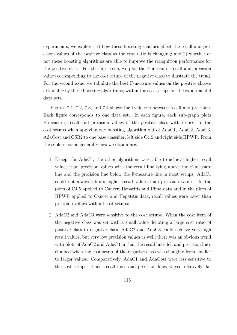
experiments, we explore: 1) how these boosting schemes affect the recall and pre-
cision values of the positive class as the cost ratio is changing; and 2) whether or
not these boosting algorithms are able to improve the recognition performance for
the positive class. For the first issue, we plot the F-measure, recall and precision
values corresponding to the cost setups of the negative class to illustrate the trend.
For the second issue, we tabulate the best F-measure values on the positive classes
attainable by these boosting algorithms, within the cost setups for the experimental
data sets.
Figures 7.1, 7.2, 7.3, and 7.4 shows the trade-offs between recall and precision.
Each figure corresponds to one data set. In each figure, each sub-graph plots
F-measure, recall and precision values of the positive class with respect to the
cost setups when applying one boosting algorithm out of AdaC1, AdaC2, AdaC3,
AdaCost and CSB2 to one base classifier, left side C4.5 and right side HPWR. From
these plots, some general views we obtain are:
1. Except for AdaC1, the other algorithms were able to achieve higher recall
values than precision values with the recall line lying above the F-measure
line and the precision line below the F-measure line in most setups. AdaC1
could not always obtain higher recall values than precision values. In the
plots of C4.5 applied to Cancer, Hepatitis and Pima data and in the plots of
HPWR applied to Cancer and Hepatitis data, recall values were lower than
precision values with all cost setups;
2. AdaC2 and AdaC3 were sensitive to the cost setups. When the cost item of
the negative class was set with a small value denoting a large cost ratio of
positive class to negative class, AdaC2 and AdaC3 could achieve very high
recall values, but very low precision values as well; there was an obvious trend
with plots of AdaC2 and AdaC3 in that the recall lines fell and precision lines
climbed when the cost setup of the negative class was changing from smaller
to larger values. Comparatively, AdaC1 and AdaCost were less sensitive to
the cost setups. Their recall lines and precision lines stayed relatively flat
115

0.1 0.2 0.3 0.4 0.5 0.6 0.7 0.8 0.9
0.4
0.6
0.8
1
0.1 0.2 0.3 0.4 0.5 0.6 0.7 0.8 0.9
0.4
0.6
0.8
1
0.1 0.2 0.3 0.4 0.5 0.6 0.7 0.8 0.9
0.4
0.6
0.8
1
0.1 0.2 0.3 0.4 0.5 0.6 0.7 0.8 0.9
0.4
0.6
0.8
1
0.1 0.2 0.3 0.4 0.5 0.6 0.7 0.8 0.9
0.4
0.6
0.8
1
Per
cent
age
0.1 0.2 0.3 0.4 0.5 0.6 0.7 0.8 0.9
0.4
0.6
0.8
1
0.1 0.2 0.3 0.4 0.5 0.6 0.7 0.8 0.9
0.4
0.6
0.8
1
0.1 0.2 0.3 0.4 0.5 0.6 0.7 0.8 0.9
0.4
0.6
0.8
1
0.1 0.2 0.3 0.4 0.5 0.6 0.7 0.8 0.9
0.4
0.6
0.8
1
0.1 0.2 0.3 0.4 0.5 0.6 0.7 0.8 0.9
0.4
0.6
0.8
1
F−measure
Recall
Precision
C4.5 HPWR
AdaC1
AdaC2
AdaC3
AdaCost
CSB2
Cost Setups
Figure 7.1: F-measure, Recall and Precison values of the positive class respecting tothe cost setups of the negative class by applying AdaC1, AdaC2, AdaC3, AdaCostand CSB2 to the base learners C4.5 and HPWR on the Cancer Data
116

0.1 0.2 0.3 0.4 0.5 0.6 0.7 0.8 0.9
0.4
0.6
0.8
1
0.1 0.2 0.3 0.4 0.5 0.6 0.7 0.8 0.9
0.4
0.6
0.8
1
0.1 0.2 0.3 0.4 0.5 0.6 0.7 0.8 0.9
0.4
0.6
0.8
1
0.1 0.2 0.3 0.4 0.5 0.6 0.7 0.8 0.9
0.4
0.6
0.8
1
0.1 0.2 0.3 0.4 0.5 0.6 0.7 0.8 0.9
0.4
0.6
0.8
1
Per
cent
age
0.1 0.2 0.3 0.4 0.5 0.6 0.7 0.8 0.9
0.4
0.6
0.8
1
0.1 0.2 0.3 0.4 0.5 0.6 0.7 0.8 0.9
0.4
0.6
0.8
1
0.1 0.2 0.3 0.4 0.5 0.6 0.7 0.8 0.9
0.4
0.6
0.8
1
0.1 0.2 0.3 0.4 0.5 0.6 0.7 0.8 0.9
0.4
0.6
0.8
1
0.1 0.2 0.3 0.4 0.5 0.6 0.7 0.8 0.9
0.4
0.6
0.8
1
F−measure
Recall
Precision
Cost Setups
C4.5 HPWR
AdaC1
AdaC2
AdaC3
AdaCost
CSB2
Figure 7.2: F-measure, Recall and Precision values of the positive class respecting tothe cost setups of the negative class by applying AdaC1, AdaC2, AdaC3, AdaCostand CSB2 to the base learners C4.5 and HPWR on the Hepatitis Data
117

0.1 0.2 0.3 0.4 0.5 0.6 0.7 0.8 0.9
0.4
0.6
0.8
1
0.1 0.2 0.3 0.4 0.5 0.6 0.7 0.8 0.9
0.4
0.6
0.8
1
0.1 0.2 0.3 0.4 0.5 0.6 0.7 0.8 0.9
0.4
0.6
0.8
1
0.1 0.2 0.3 0.4 0.5 0.6 0.7 0.8 0.9
0.4
0.6
0.8
1
0.1 0.2 0.3 0.4 0.5 0.6 0.7 0.8 0.9
0.4
0.6
0.8
1
Per
cent
age
0.1 0.2 0.3 0.4 0.5 0.6 0.7 0.8 0.9
0.4
0.6
0.8
1
0.1 0.2 0.3 0.4 0.5 0.6 0.7 0.8 0.9
0.4
0.6
0.8
1
0.1 0.2 0.3 0.4 0.5 0.6 0.7 0.8 0.9
0.4
0.6
0.8
1
0.1 0.2 0.3 0.4 0.5 0.6 0.7 0.8 0.9
0.4
0.6
0.8
1
0.1 0.2 0.3 0.4 0.5 0.6 0.7 0.8 0.9
0.4
0.6
0.8
1
F−measure
Recall
Precision
C4.5 HPWR
AdaC1
AdaC2
AdaC3
AdaCost
CSB2
Cost Setups
Figure 7.3: F-measure, Recall and Precison values of the positive class respecting tothe cost setups of the negative class by applying AdaC1, AdaC2, AdaC3, AdaCostand CSB2 to the base learners C4.5 and HPWR on the Pima Data
118

0.1 0.2 0.3 0.4 0.5 0.6 0.7 0.8 0.9
0.2
0.4
0.6
0.8
1
0.1 0.2 0.3 0.4 0.5 0.6 0.7 0.8 0.9
0.2
0.4
0.6
0.8
1
0.1 0.2 0.3 0.4 0.5 0.6 0.7 0.8 0.9
0.2
0.4
0.6
0.8
1
0.1 0.2 0.3 0.4 0.5 0.6 0.7 0.8 0.9
0.2
0.4
0.6
0.8
1
0.1 0.2 0.3 0.4 0.5 0.6 0.7 0.8 0.9
0.2
0.4
0.6
0.8
1
Per
cent
age
0.1 0.2 0.3 0.4 0.5 0.6 0.7 0.8 0.9
0.2
0.4
0.6
0.8
1
0.1 0.2 0.3 0.4 0.5 0.6 0.7 0.8 0.9
0.2
0.4
0.6
0.8
1
0.1 0.2 0.3 0.4 0.5 0.6 0.7 0.8 0.9
0.2
0.4
0.6
0.8
1
0.1 0.2 0.3 0.4 0.5 0.6 0.7 0.8 0.9
0.2
0.4
0.6
0.8
1
0.1 0.2 0.3 0.4 0.5 0.6 0.7 0.8 0.9
0.2
0.4
0.6
0.8
1
F−measure
Recall
Precision
C4.5 HPWR
AdaCost
AdaC2
AdaC3
AdaC1
CSB2
Cost Setups
Figure 7.4: F-measure, Recall and Precision values of the positive class respecting tothe cost setups of the negative class by applying AdaC1, AdaC2, AdaC3, AdaCostand CSB2 to the base learners C4.5 and HPWR on the Sick Data
119

when the cost setup was changing. CSB2 produced values oscillating slightly
as the cost setup was changing.
3. Comparing AdaCost with AdaC1, recall values of AdaCost were higher than
those of AdaC1 in most cases.
These observations are consistent with the analysis of the resampling effects
of these boosting algorithms. AdaC1, AdaC2 and AdaC3 all boost more weights
on False Negatives than those on False Positives; on the correctly classified part,
AdaC1 decreas weights of True Positives more than those of True Negatives, AdaC2
preserve more weights of True Positives than those of True Negatives. Therefore,
AdaC1 conserve more weights on the negative class, AdaC2 boost more weights to-
wards the positive class, and AdaC3 is a combinational result of AdaC1 and AdaC2.
These analyses account for the observation that AdaC2 and AdaC3 achieved higher
recall values than AdaC1. AdaCost [29] is a variation of AdaC1, in that it intro-
duces a cost adjustment function instead of a cost item inside the exponential
function. The cost adjustment function increases its weight “more” if misclassified
and decreases the weight “less” otherwise. AdaCost therefore boosted more weights
on the positive class than AdaC1. As a result, recall values obtained by AdaCost
were usually higher than those of AdaC1. CSB2 increased weights more on False
Negatives than False Positives, but decreased weights on true predictions equally.
After normalization, it was not always guaranteed that the overall boosted weights
on the positive class were more than those on the negative class, as samples of the
positive class were few.
Table 7.6 shows the best F-measure values achieved by each boosting algo-
rithm and the cost settings with which these values were achieved. To indicate
at what recall and precision values these F-measure values were achieved, we also
list the corresponding recall and precision values of the positive class. In these
tables, “F” denotes F-measure, “R” recall and “P” precision of the positive class.
Comparing with the F-measure (on the positive class) values obtained by the base
classifications, those significantly better F-measure values through t-test with 95%
120

Table 7.6: F-measure Comparisons
Base AdaBoost AdaC1 AdaC2 AdaC3 AdaCost CSB2Cost 1:0.9 1:0.6 1:0.6 1:0.4 1:0.1
F 39.51 42.60 44.77 48.22 49.81 48.72 48.31C4.5 R 34.53 39.25 41.86 56.45 56.65 54.92 65.10
Cancer P 47.92 48.36 50.18 42.28 44.76 44.81 40.37Data Cost 1:0.9 1:0.7 1:0.6 1:0.2 1:0.4
F 41.44 46.44 50.70 53.98 54.97 50.75 50.73HPWR R 44.17 44.68 49.06 70.80 83.45 59.50 66.98Od=6 P 40.91 49.58 54.18 44.61 41.44 44.64 41.04
Cost 1:0.1 1:0.5 1:0.8 1:0.8 1:0.8F 50.89 55.87 61.39 71.63 70.13 62.05 60.55
C4.5 R 53.84 53.98 64.20 77.89 66.78 60.85 61.60Hepa P 50.08 69.56 60.86 70.16 74.94 63.29 59.53Data Cost 1:0.6 1:0.7 1:0.7 1:0.7 1:0.9
F 56.45 61.86 63.59 65.19 62.88 61.93 58.51HPWR R 68.68 59.23 60.86 81.73 75.99 64.67 64.23Od=3 P 52.20 66.93 71.11 57.02 56.77 61.29 56.20
Cost 1:0.6 1:0.9 1:0.9 1:0.3 1:0.7F 64.98 65.61 66.17 68.69 68.29 67.77 64.98
C4.5 R 59.57 60.42 61.40 82.52 81.99 83.75 59.96Pima P 72.26 72.55 71.75 59.15 58.69 57.11 71.81Data Cost 1:0.3 1:0.7 1:0.6 1:0.3 1:0.9
F 67.98 68.17 72.59 71.03 73.36 69.05 65.58HPWR R 70.97 68.85 81.15 80.94 80.89 76.33 68.55Od=4 P 65.52 67.77 65.83 63.49 67.25 63.40 64.22
Cost 1:0.5 1:0.9 1:0.9 1:0.7 1:0.9F 84.79 84.04 85.31 82.38 83.53 83.46 79.18
C4.5 R 83.87 82.96 84.75 83.46 84.26 84.74 80.57Sick P 85.73 85.19 86.03 81.46 82.97 82.45 79.15Data Cost 1:0.9 1:0.9 1:0.8 1:0.9 1:0.6
F 69.22 79.77 86.36 78.05 81.04 82.67 64.88HPWR R 70.89 80.99 86.36 83.19 86.85 87.11 71.05Od=3 P 68.30 79.08 76.15 73.44 76.01 78.78 59.96
confidence interval are presented in italics and the best results with respect to each
base classifier applied to a data set are denoted in bold.
Comparing with the base classifications on the Cancer data, most cost-sensitive
boosting algorithms obtained significantly better F-measure values except AdaC1
when applied to C4.5. On the Hepatitis data, when applied to C4.5, all cost-
121

sensitive boosting algorithms achieved significantly better F-measure values; when
applied to HPWR, AdaC1, AdaC2 and AdaC3 obtained significantly better F-
measure values. On the Pima data, AdaC1 and AdaC3 when applied to HPWR
got significantly better results. On the Sick data, except CSB2, the other boosting
algorithms including AdaBoost achieved significantly better values when applied on
HPWR. Taking one base classifier associated with one data set as one entity, among
these 8 entities (2 base classifier crossing with 4 data sets), AdaBoost achieved
significantly better results on 1 entity, AdaC1 on 4 entities, AdaC2 on 5 entities,
AdaC3 on 6 entities, AdaCost on 4 entities and CSB2 on 3 entities. For the best
performance out of the 8 entities, AdaC1 won 2 times, and AdaC2 and AdaC3 both
won 3 times.
7.2.4 G-mean Evaluation
G-mean is defined as the geometric mean of True Positive Rate and True Negative
Rate (Equation 2.6). True Positive Rate denotes recall of the positive class and
True Negative Rate denotes the recall of the negative class. With the class imbal-
ance problem, recall of the positive class is often very low. Cost-sensitive boosting
algorithms deliberately boost more weights towards the positive class to improve
recognition recall. However, if the positive class is over-boosted, samples from the
negative class will be mis-categorized to the positive class. Consequently, recall of
the negative class will be reduced. G-mean reflects the idea of maximizing the recall
on each of the two classes while keeping these recall values balanced. In this part of
the experiments, we explore: 1) how these boosting schemes affect the recall values
of positive class and negative class as the cost ratio is changing; and 2) whether or
not these boosting algorithms were able to improve the G-mean measurements by
increasing the recall values of the positive class. As in the previous section, we use
figures to illustrate the first issue and use a table to clarify the second issue.
Figures 7.5, 7.6, 7.7, and 7.8 show the trade-offs between recall values of the
positive class and the negative class. As before, each figure corresponds to one
data set. In each figure, a sub-graph plots G-mean values, recall values of both the
122

0.1 0.2 0.3 0.4 0.5 0.6 0.7 0.8 0.90
0.2
0.4
0.6
0.8
1
0.1 0.2 0.3 0.4 0.5 0.6 0.7 0.8 0.90
0.2
0.4
0.6
0.8
1
0.1 0.2 0.3 0.4 0.5 0.6 0.7 0.8 0.90
0.2
0.4
0.6
0.8
1
0.1 0.2 0.3 0.4 0.5 0.6 0.7 0.8 0.90
0.2
0.4
0.6
0.8
1
0.1 0.2 0.3 0.4 0.5 0.6 0.7 0.8 0.90
0.2
0.4
0.6
0.8
1
Per
cent
age
0.1 0.2 0.3 0.4 0.5 0.6 0.7 0.8 0.90
0.2
0.4
0.6
0.8
1
0.1 0.2 0.3 0.4 0.5 0.6 0.7 0.8 0.90
0.2
0.4
0.6
0.8
1
0.1 0.2 0.3 0.4 0.5 0.6 0.7 0.8 0.90
0.2
0.4
0.6
0.8
1
0.1 0.2 0.3 0.4 0.5 0.6 0.7 0.8 0.90
0.2
0.4
0.6
0.8
1
0.1 0.2 0.3 0.4 0.5 0.6 0.7 0.8 0.90
0.2
0.4
0.6
0.8
1
G−mean
Positive Recall
Negative Recall
C4.5 HPWR
AdaC1
AdaC2
AdaC3
AdaCost
CSB2
Cost Setups
Figure 7.5: G-mean values, Recall values of both the positive class and negativeclass respecting to the cost setups of the negative class by applying AdaC1, AdaC2,AdaC3, AdaCost and CSB2 to the base learners C4.5 and HPWR on the CancerData
123

0.1 0.2 0.3 0.4 0.5 0.6 0.7 0.8 0.90
0.5
1
0.1 0.2 0.3 0.4 0.5 0.6 0.7 0.8 0.90
0.5
1
0.1 0.2 0.3 0.4 0.5 0.6 0.7 0.8 0.90
0.5
1
0.1 0.2 0.3 0.4 0.5 0.6 0.7 0.8 0.90
0.5
1
0.1 0.2 0.3 0.4 0.5 0.6 0.7 0.8 0.90
0.5
1
perc
enta
ge
0.1 0.2 0.3 0.4 0.5 0.6 0.7 0.8 0.90
0.5
1
0.1 0.2 0.3 0.4 0.5 0.6 0.7 0.8 0.90
0.5
1
0.1 0.2 0.3 0.4 0.5 0.6 0.7 0.8 0.90
0.5
1
0.1 0.2 0.3 0.4 0.5 0.6 0.7 0.8 0.90
0.5
1
0.1 0.2 0.3 0.4 0.5 0.6 0.7 0.8 0.90
0.5
1
G−mean
Positive Recall
Negative Recall
C4.5 HPWR
AdaC1
AdaC2
AdaC3
AdaCost
CSB2
Cost Setups
Figure 7.6: G-mean values, Recall values of both the positive class and negativeclass respecting to the cost setups of the negative class by applying AdaC1, AdaC2,AdaC3, AdaCost and CSB2 to the base learners C4.5 and HPWR on the HepatitisData
124
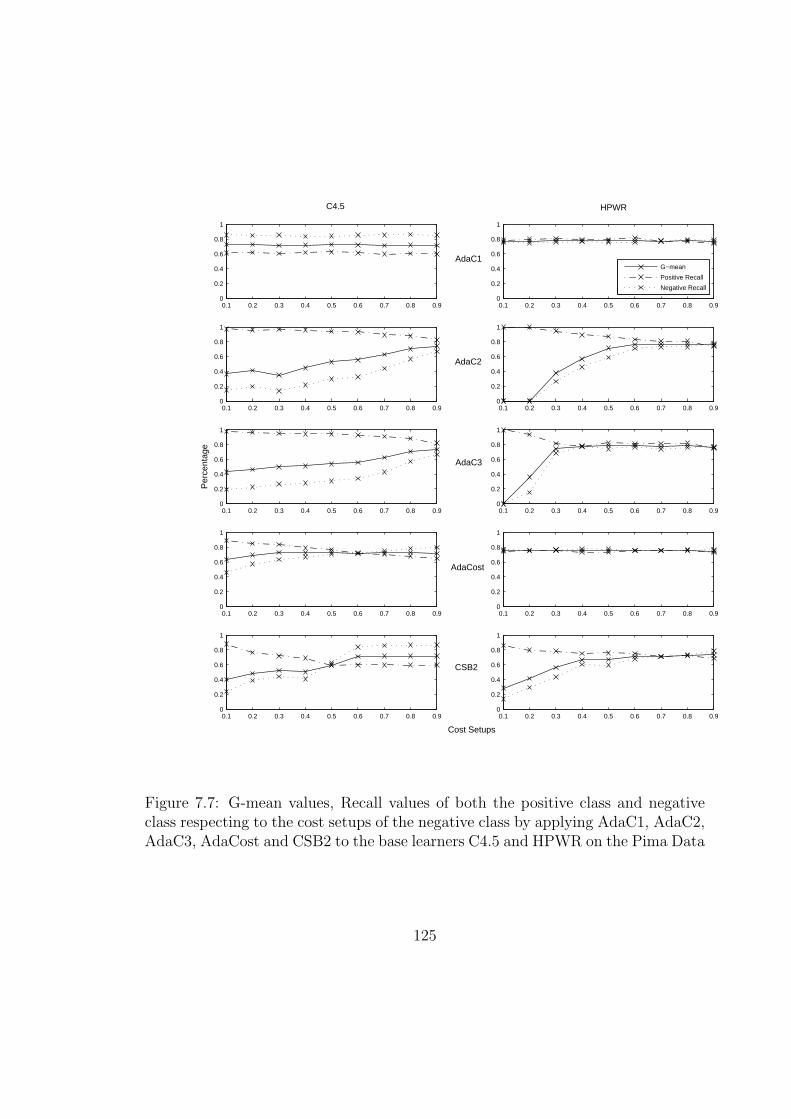
0.1 0.2 0.3 0.4 0.5 0.6 0.7 0.8 0.90
0.2
0.4
0.6
0.8
1
0.1 0.2 0.3 0.4 0.5 0.6 0.7 0.8 0.90
0.2
0.4
0.6
0.8
1
0.1 0.2 0.3 0.4 0.5 0.6 0.7 0.8 0.90
0.2
0.4
0.6
0.8
1
0.1 0.2 0.3 0.4 0.5 0.6 0.7 0.8 0.90
0.2
0.4
0.6
0.8
1
0.1 0.2 0.3 0.4 0.5 0.6 0.7 0.8 0.90
0.2
0.4
0.6
0.8
1
Per
cent
age
0.1 0.2 0.3 0.4 0.5 0.6 0.7 0.8 0.90
0.2
0.4
0.6
0.8
1
0.1 0.2 0.3 0.4 0.5 0.6 0.7 0.8 0.90
0.2
0.4
0.6
0.8
1
0.1 0.2 0.3 0.4 0.5 0.6 0.7 0.8 0.90
0.2
0.4
0.6
0.8
1
0.1 0.2 0.3 0.4 0.5 0.6 0.7 0.8 0.90
0.2
0.4
0.6
0.8
1
0.1 0.2 0.3 0.4 0.5 0.6 0.7 0.8 0.90
0.2
0.4
0.6
0.8
1
G−mean
Positive Recall
Negative Recall
C4.5 HPWR
AdaC1
AdaC2
AdaC3
AdaCost
CSB2
Cost Setups
Figure 7.7: G-mean values, Recall values of both the positive class and negativeclass respecting to the cost setups of the negative class by applying AdaC1, AdaC2,AdaC3, AdaCost and CSB2 to the base learners C4.5 and HPWR on the Pima Data
125
0.1 0.2 0.3 0.4 0.5 0.6 0.7 0.8 0.9
0.2
0.4
0.6
0.8
1
0.1 0.2 0.3 0.4 0.5 0.6 0.7 0.8 0.9
0.2
0.4
0.6
0.8
1
0.1 0.2 0.3 0.4 0.5 0.6 0.7 0.8 0.9
0.2
0.4
0.6
0.8
1
0.1 0.2 0.3 0.4 0.5 0.6 0.7 0.8 0.9
0.2
0.4
0.6
0.8
1
0.1 0.2 0.3 0.4 0.5 0.6 0.7 0.8 0.9
0.2
0.4
0.6
0.8
1
Per
cent
age
0.1 0.2 0.3 0.4 0.5 0.6 0.7 0.8 0.9
0.2
0.4
0.6
0.8
1
0.1 0.2 0.3 0.4 0.5 0.6 0.7 0.8 0.9
0.2
0.4
0.6
0.8
1
0.1 0.2 0.3 0.4 0.5 0.6 0.7 0.8 0.9
0.2
0.4
0.6
0.8
1
0.1 0.2 0.3 0.4 0.5 0.6 0.7 0.8 0.9
0.2
0.4
0.6
0.8
1
0.1 0.2 0.3 0.4 0.5 0.6 0.7 0.8 0.9
0.2
0.4
0.6
0.8
1
G−mean
Positive Recall
Negative Recall
C4.5 HPWR
AdaC1
AdaC2
AdaC3
AdaCost
CSB2
Cost Setups
Figure 7.8: G-mean values, Recall values of both the positive class and negativeclass respecting to the cost setups of the negative class by applying AdaC1, AdaC2,AdaC3, AdaCost and CSB2 to the base learners C4.5 and HPWR on the Sick Data
126

positive class and the negative class with respect to the cost setups when applying
one boosting algorithm out of AdaC1, AdaC2, AdaC3, AdaCost and CSB2 to
one base classifier, left side C4.5 and right side HPWR. The observations are: 1)
AdaC1 and AdaCost usually achieved higher negative recall values than positive
recall values with their positive recall lines lying below and negative lines lying
above their G-mean lines in most cases; 2) there was an obvious trend with plots of
AdaC2 and AdaC3, in that the positive recall lines fell and the negative recall lines
climbed with the cost setup changing from smaller values to larger values. With
small cost setups of the negative class, positive recall lines were above negative
recall lines. These two lines later intersected at a certain cost setup, and then
negative recall lines lay above the positive recall lines. Lines of CSB2 also showed
this trend, but oscillated in some cases. These observations were consistent with
the analysis of the resampling effects of the boosting algorithms as discussed in the
previous section.
Table 7.7 shows the best G-mean values achieved by each boosting algorithm
and the cost settings with which these values were achieved. The corresponding
recall values of the two classes are also listed. In these tables, “G” denotes G-mean,
“R+” recall of the positive class and “R−” recall of the negative class. Comparing
with the G-mean values obtained by the base classifications, those significantly
better G-mean values through t-test with a 95% confidence interval are presented
in italics and the best results of each base classifier when applied to a data set are
denoted in bold. The resulting table furnished the same features as those in Table
7.6.
7.3 Classification of Multi-Class Imbalanced Data
In this section, we set up experiments to investigate the cost-sensitive boosting
algorithm AdaC2.M1 with respect to its capability in dealing with the multi-class
imbalance problem. Both AdaBoost.M1 and AdaC2.M1 were applied to the de-
cision tree classification system C4.5 and the associative classifier HPWR. Their
127

Table 7.7: G-mean Comparison
Base AdaBoost AdaC1 AdaC2 AdaC3 AdaCost CSB2Cost 1:0.9 1:0.6 1:0.6 1:0.4 1:0.9G 53.21 56.19 57.81 61.12 62.79 61.90 57.88
C4.5 R+ 34.53 39.25 41.86 56.45 56.65 54.92 50.17Cancer R− 83.27 82.00 82.01 66.78 69.87 70.94 68.17Data Cost 1:0.7 1:0.9 1:0.9 1:0.2 1:0.4
G 55.78 59.36 63.64 65.51 65.99 65.00 64.83HPWR R+ 44.17 44.68 51.54 60.95 56.13 59.50 66.98Od=6 R− 71.91 79.40 78.94 71.24 65.99 71.92 63.22
Cost 1:0.1 1:0.5 1:0.2 1:0.7 1:0.8G 65.92 68.86 73.00 83.57 79.13 75.97 71.72
C4.5 R+ 53.84 53.98 64.20 77.89 76.46 65.59 61.60Hepa R− 85.32 91.90 86.23 91.33 84.04 89.31 85.68Data Cost 1:0.1 1:0.7 1:0.6 1:0.6 1:0.4
G 74.21 72.22 74.54 82.37 81.38 74.49 74.77HPWR R+ 68.68 59.23 64.23 81.73 85.80 65.30 71.64Od=3 R− 82.79 90.29 88.28 83.37 79.38 87.90 82.91
Cost 1:0.2 1:0.9 1:0.9 1:0.5 1:0.7G 71.70 72.23 72.68 74.08 73.62 73.66 71.69
C4.5 R+ 59.57 60.42 62.19 82.52 81.99 76.91 59.96Pima R− 86.79 86.72 85.25 66.85 66.43 70.67 86.27Data Cost 1:0.3 1:0.7 1:0.6 1:0.3 1:0.9
G 75.23 75.33 78.42 76.85 78.92 76.09 73.27HPWR R+ 70.97 68.85 81.15 80.94 80.89 76.33 68.55Od=4 R− 79.94 82.50 75.87 73.15 77.07 76.12 78.98
Cost 1:0.5 1:0.8 1:0.9 1:0.5 1:0.9G 90.95 90.37 91.37 90.95 90.94 91.20 88.25
C4.5 R+ 83.87 82.96 84.75 84.93 84.26 84.94 80.57Sick R− 98.54 98.49 98.55 97.46 98.21 97.97 96.84Data Cost 1:0.8 1:0.7 1:0.8 1:0.8 1:0.6
G 82.57 88.83 91.52 90.65 91.79 92.42 82.00HPWR R+ 70.89 80.99 85.84 86.30 86.85 88.04 71.05Od=3 R− 96.38 97.58 97.60 95.35 97.03 97.04 94.80
performances on data sets with multiple classes where the imbalanced class dis-
tributions hindered the classification performances of the base classifications were
compared and analyzed. The Genetic Algorithm was implemented to search the
cost setups for applying AdaC2.M1.
Four data sets Balance-Scale data, Car data, New-thyroid data and Nursery
128

data were taken from the UCI Machine Learning Database [64] for our experiments.
Given a multi-class data set with imbalanced class distribution, the identification
performances of the small classes are usually unsatisfactory. To remedy this, the
learning objective can be: 1) to balance the identification abilities over every class;
and/or 2) to improve the recognition success on a specific small class. With re-
spect to the different learning objectives, the classification performance should be
evaluated by different measures.
7.3.1 Evaluation Measures
Referring to the confusion matrix of Table 6.1, the true prediction of the ith class is
the number of nii. If the learning objective is to improve the identification ability
of a specific class, the evaluation measure is F-measure. Let Ri and Pi denote recall
and precision, respectively, of class Ci , Ri and Pi are then defined as:
Ri =nii∑k
j=1 nij
(7.1)
and
Pi =nii∑k
j=1 nji
(7.2)
F-measure (F) is then calculated as an average:
Fi −measure =2RiPi
Ri + Pi
(7.3)
If the learning objective is to balance the identification performances among
classes, the classification performance of each class should be equally represented
in the evaluation measure. For the bi-class scenario, Kubat et al [53] suggested
the G-mean as the geometric means to recall values of two classes. Expanding this
measure to the multiple class scenario, we define G-mean as the geometric means
of recall values to all classes:
129

G−mean =
(k∏
i=1
Ri
)1/k
(7.4)
As each recall value representing the classification performance of a specific class
is equally represented, G-mean is capable of measuring the balanced performance
among classes of a classification output.
F-measure (Equation 7.3) and G-mean (Equation 7.4) are used in evaluating
and comparing the classification performance, as well as the fitness functions by the
Genetic Algorithm when searching for efficient cost setups with respect to different
learning objectives.
7.3.2 Experiment Method
For each data set, available samples were used for both cost setup searching and
performance evaluation. Normally in such a case, the data needs to be partitioned
into three disjoint sets: 1) training set, a set of examples used for learning classi-
fication model; 2) validation set, a set of examples used to tune the parameters of
the cost values; and 3) test set, a set of examples used to assess the performance.
Performance is evaluated by k-fold cross validations. In our case, however, avail-
able data examples, mainly examples of the small classes, are insufficient for so
many partitions. For this reason, we employed two sections of partitions. The first
section of partitions was for searching cost setups by the GA. The data set was
randomly divided into two sets: 80% as the training set and the remaining 20% as
the validation set for measuring the fitness of a bunch of cost setups generated by
the GA. The output was a cost vector which obtains the best fitness value among
all tests. This process was repeated 20 times, such that one prototype was obtained
from a pool of 20 cost vectors. In these experiments, we used the default parame-
ters for the GA: population size was 50; generation number was 20; mutation rate
was 0.2; crossover rate was 0.8; and migration rate was 0.2. The second section of
partitions, totally independent from the first section, was for evaluating the classi-
fication performance. The whole data set was repartitioned into two sets: 80% as
130

�
������������
����� �����������
��������������������� ���������������������
��������
�����
�������������
����
���!���������
������ �����
����������������"���
��������
�����
�������������
����
���������
�!���#$�� �!�%��#$�� %����
Figure 7.9: Experiment Procedure
the training set and the remaining 20% as the test set. This process was repeated
10 times to obtain an average performance. For a consistent comparison, the bases
classification models C4.5 and HPWR, base classifiers applied by AdaBoost.M1 and
by AdaC2.M1, were all evaluated on data partitions of the second section. This
procedure is described in Figure 7.9
The cost setup used by AdaC2.M1 was the prototype from the validation tests
with the first section of partitions. In our experiments, we took the mean of a
pool of 20 cost vectors as the cost setup prototype. As stated in [26], given a set
of cost setups, the ratios among cost values denote the deviations of the learning
importance among classes. The decisions are unchanged if each one in the set is
multiplied by a positive constant. Therefore, to set up a unique scale, normalizing
each cost vector in the pool is a necessary step before calculating the mean values.
The normalization method was, first, to set the value of the element with the
maximum value in a vector as 1, then, to scale other elements’ values in the vector
131
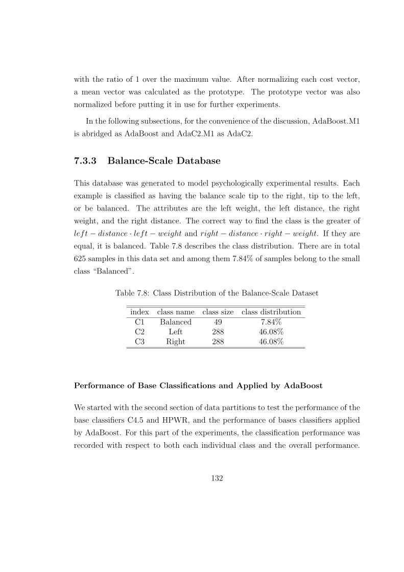
with the ratio of 1 over the maximum value. After normalizing each cost vector,
a mean vector was calculated as the prototype. The prototype vector was also
normalized before putting it in use for further experiments.
In the following subsections, for the convenience of the discussion, AdaBoost.M1
is abridged as AdaBoost and AdaC2.M1 as AdaC2.
7.3.3 Balance-Scale Database
This database was generated to model psychologically experimental results. Each
example is classified as having the balance scale tip to the right, tip to the left,
or be balanced. The attributes are the left weight, the left distance, the right
weight, and the right distance. The correct way to find the class is the greater of
left − distance · left − weight and right − distance · right − weight. If they are
equal, it is balanced. Table 7.8 describes the class distribution. There are in total
625 samples in this data set and among them 7.84% of samples belong to the small
class “Balanced”.
Table 7.8: Class Distribution of the Balance-Scale Dataset
index class name class size class distributionC1 Balanced 49 7.84%C2 Left 288 46.08%C3 Right 288 46.08%
Performance of Base Classifications and Applied by AdaBoost
We started with the second section of data partitions to test the performance of the
base classifiers C4.5 and HPWR, and the performance of bases classifiers applied
by AdaBoost. For this part of the experiments, the classification performance was
recorded with respect to both each individual class and the overall performance.
132

Regarding each class, recall value, precision value and F-measure value were re-
ported. Regarding the overall performance, the classification accuracy and G-mean
value were calculated. Experiment results are tabulated in Table 7.9.
Table 7.9: Performance of Base Classifications and Applied by AdaBoost
C4.5 HPWR (Od=3)Class Meas. Base AdaBoost Base AdaBoost
R 0 5.11 10.70 44.06C1 P N/A 6.5 11.82 32.89
F N/A 5.84 10.83 35.84R 73.21 92.28 88.31 87.43
C2 P 69.53 88.75 86.79 91.99F 72.29 90.38 87.43 89.64R 67.94 91.36 87.63 88.42
C3 P 73.89 87.88 87.07 89.91F 71.91 89.42 86.99 89.03
Accuracy 70.33 85.77 83.35 86.68G-mean 0 11.46 33.32 68.50
In this table, “F” denotes F-measure, “R” recall and “P” precision; “Od” is
the order limitation of association patterns for constructing the HPWR classifier.
Taking a look at the results, we find that: 1) with respect to the decision tree
classification system C4.5, the base classification for the small class C1 was poor,
as no relevant samples were identified, and performance for class C2 and C3 was
much better. Since the recall value of class C1 was zero, G-mean value was also
zero. By applying the AdaBoost algorithm, very few samples of the small class were
correctly classified, and performance for class C2 and C3 was significantly improved.
The overall classification accuracy was also significantly improved, however, the G-
mean value kept very low as a result of a low recall value for class C1; and 2) with
respect to the associative classification system HPWR, the base classification for the
small class C1 was poor with very low recall, precision and F-measure values, while
these values of the other two classes were much higher. By applying AdaBoost,
133
even though F-measure values of all classes were improved, that of the small class
C1 was far below those of the other two classes. The overall performance accuracy
and G-mean were all improved accordingly.
These observations indicated the poor performance for the small class of both
base classifications and those applied by AdaBoost. We since expected to improve
the performance for the small class C1. By applying AdaC2, two learning objectives
were: 1) to balance the classification performance among classes evaluated by G-
mean; and 2) to improve the identification ability on class C1 evaluated by F-
measure.
G-mean Evaluation
We ran GA for searching efficient cost setups with data partitions of the first section.
With respect to the first learning objective, the fitness function was G-mean. The
resulting prototype of a cost vector [1.00 0.6331 0.6438] was specific to C4.5 and
another one [1.00 0.8120 0.8512] was for HPWR. The common feature of these
two vectors was that a higher cost value was assigned to the small class C1 and
relatively lower and similar values were associated with the other two classes. This
format was consistent with the learning expectation to strengthen the small class
C1. Integrating these cost vectors into AdaC2, its performance was evaluated by the
data partitions of the second section. Table 7.10 tabulates results for comparing the
performances of base classification, applied by classification, applied by AdaBoost,
and applied by AdaC2 in terms of their abilities in balancing the performances
among classes.
G-mean is calculated as the geometric means of recall values of all classes. For
each class crossing with each learning algorithm, the recall value, as well as the
precision value (in italics), are tabulated. G-mean values are presented in bold.
Comparing classification performances of the base classifications C4.5 and HPWR,
applied by AdaBoost, and applied by AdaC2, AdaC2 achieved the best G-mean
values. With respect to each class, AdaC2 improved recall values of the small class
134

Table 7.10: G-mean Evaluation
C4.5 HPWR (Od=3)Class Meas. Base AdaBoost AdaC2 Base AdaBoost AdaC2C1 R 0 5.11 77.58 10.70 44.06 65.72
P N/A 6.50 14.12 11.82 32.89 30.83C2 R 73.21 92.28 64.73 88.31 87.43 83.12
P 69.53 88.75 97.24 86.79 91.99 91.38C3 R 67.94 91.36 65.23 87.63 88.42 83.95
P 73.89 87.88 93.22 87.07 89.91 90.81G-mean 0 11.46 68.42 33.32 68.50 76.08
Cost Vector [1.00 0.6331 0.6438 ] [1.00 0.8120 0.8512]
significantly, while at the same time, decreased recall values of the other two classes
accordingly, more by C4.5 and less by HPWR.
F-measure Evaluation
With respect to the second learning objective, the fitness function was F-measure
evaluation on class C1. The resulting prototype cost vectors were [1.00 0.7597 0.7518]
for C4.5 and [1.00 0.9469 0.9934] for HPWR. Again, they took the same format
of a higher cost value associated with the small class C1 and relatively lower and
similar values to the other two classes. Integrating this cost vector to AdaC2, the
classification performance of class C1 was evaluated by the data partitions of the
second section. Table 7.11 presents the results.
With respect to class C1 crossing each learning algorithm, recall (R), precision
(P) and F-measure (F) values are reported, with F-measure values presented in
bold type. For reference of the performances on the other two classes, these values
are presented in italics. Applying AdaC2 to both classification systems C4.5 and
HPWR, the common observation is that AdaC2 achieved the best F-measure values
by improving the recall values and preserving higher precision values as well on class
C1, as compared with the base classifications and applied by AdaBoost.
135

Table 7.11: F-measure Evaluation on Class C1
C4.5 HPWR (Od=3)Class Meas. Base AdaBoost AdaC2 Base AdaBoost AdaC2
R 0 5.11 54.31 10.70 44.06 50.92C1 P N/A 6.50 16.03 11.82 32.89 34.35
F N/A 5.84 24.25 10.83 35.84 39.78R 73.21 92.28 78.19 88.31 87.43 88.05
C2 P 69.53 88.75 92.54 86.79 91.99 90.94F 72.29 90.38 84.41 87.43 89.64 89.43R 67.94 91.36 75.00 87.63 88.42 86.68
C3 P 73.89 87.88 92.95 87.07 89.91 90.38F 71.91 89.42 83.01 86.99 89.03 88.42
Cost Vector [1.00 0.7597 0.7518 ] [1.00 0.9469 0.9934]
When comparing the reported results achieved by applying AdaC2 in Table 7.11
with those in Table 7.10, some interesting points are noticed. With respect to each
classification system, C4.5 or HPWR, the two cost vectors searched by GA for Table
7.11 and Table 7.10 were in the same format: a higher cost value was associated
with the small class C1 and relatively lower and similar values were associated with
the other two classes. However, the ratios between cost values for Table 7.11 were
smaller than those for Table 7.10. Hence, class C1 achieved relatively lower cost
values in Table 7.11 than in Table 7.10. Consequently, recall values of class C1
in Table 7.11 were lower than those in Table 7.10, and precision values were in
the contrary situation. These might result from the fact that a higher F-measure
should balance the trade-offs between recall and precision values. A relatively lower
cost value on the small class restrained a higher recall value, but preserved a higher
precision performance at the same time. This observation indicates how the cost
setups employed by AdaC2 adjust the learning focus and influence the classification
performances among classes.
136

7.3.4 Car Evaluation Database
This database was derived for car evaluation. There are 1728 instances with each
described by 6 nominal ordered attributes. All data are grouped into 4 classes.
Table 7.12 describes the class distribution. Class C3 and C4 are small classes with
only 3.993% and 3.762% of the entire samples, respectively.
Table 7.12: Class Distribution of the Car Dataset
index class name class size class distributionC1 unacc 1210 70.023%C2 acc 384 22.222%C3 good 69 3.993%C4 v-good 65 3.762%
Performance of Base Classifications and Applied by AdaBoost
Testing on the second section of data partitions evaluated the performance of the
base classifiers C4.5 and HPWR, and applied by AdaBoost. Experimental results
are tabulated in Table 7.13.
With respect to the classification systems of C4.5, base classification performed
significantly better on classes C1 and C2 than on the two small classes C3 and C4
in terms of F-measure values. By applying AdaBoost, performances of class C1 and
C2 retained similar values; that of class C4 was significantly improved; and that
of class C3 was also improved but far below the other classes. As for the overall
performance, the classification accuracy of C4.5 was improved slightly; G-mean
value was improved by 4.22%. With respect to the classification systems HPWR,
base classification achieved the best F-measure value on class C1, which numbered
a major size of the whole data set, and obtained poor F-measure values on the two
small classes C3 and C4. By applying AdaBoost, F-measure values on all the 4
classes were slightly improved. However, performance on class C3 was far below
137
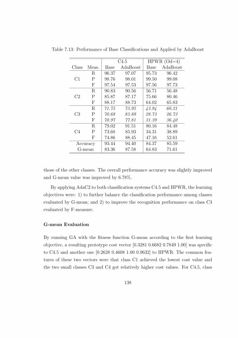
Table 7.13: Performance of Base Classifications and Applied by AdaBoost
C4.5 HPWR (Od=4)Class Meas. Base AdaBoost Base AdaBoost
R 96.37 97.07 95.73 96.42C1 P 98.76 98.01 99.50 99.08
F 97.54 97.53 97.56 97.73R 90.83 90.56 56.71 56.48
C2 P 85.87 87.17 75.66 80.46F 88.17 88.73 64.02 65.83R 71.75 73.95 43.94 60.21
C3 P 70.68 83.89 28.73 26.73F 70.97 77.81 31.39 36.40R 79.02 91.51 80.16 84.48
C4 P 73.68 85.93 34.31 38.89F 74.86 88.45 47.16 52.61
Accuracy 93.44 94.40 84.37 85.59G-mean 83.36 87.58 64.83 71.61
those of the other classes. The overall performance accuracy was slightly improved
and G-mean value was improved by 6.78%.
By applying AdaC2 to both classification systems C4.5 and HPWR, the learning
objectives were: 1) to further balance the classification performance among classes
evaluated by G-mean; and 2) to improve the recognition performance on class C3
evaluated by F-measure.
G-mean Evaluation
By running GA with the fitness function G-mean according to the first learning
objective, a resulting prototype cost vector [0.3281 0.6682 0.7849 1.00] was specific
to C4.5 and another one [0.2628 0.4608 1.00 0.9632] to HPWR. The common fea-
tures of these two vectors were that class C1 achieved the lowest cost value and
the two small classes C3 and C4 got relatively higher cost values. For C4.5, class
138

C4 achieved the highest cost value and, for HPWR, though C3 achieved the high-
est value, cost values for C3 and C4 were similar. Integrating these cost vectors
into AdaC2, its performances in terms of its abilities in balancing the performances
among classes were compared with those of base classifications and AdaBoost. Ta-
ble 7.14 tabulates these results.
Table 7.14: G-mean Evaluation
C4.5 HPWR (Od=4)Class Meas. Base AdaBoost AdaC2 Base AdaBoost AdaC2C1 R 96.37 97.07 95.86 95.73 96.42 89.06
P 98.76 98.01 98.81 99.50 99.08 99.85C2 R 90.83 90.56 94.59 56.71 56.48 79.26
P 85.87 87.17 87.61 75.66 80.46 70.77C3 R 71.75 73.95 85.40 43.94 60.21 74.15
P 70.68 83.89 84.92 28.73 26.73 45.70C4 R 79.02 91.51 91.39 80.16 84.48 96.88
P 73.68 85.93 87.77 34.31 38.89 55.62G-mean 83.36 87.58 91.46 64.83 71.61 84.20
Cost Vector [0.3281 0.6682 0.7849 1.00] [0.2628 0.4608 1.00 0.9632]
By applying to both classification systems C4.5 and HPWR, AdaC2 obtained
the best G-mean values as compared with the base classification and applied by
AdaBoost. With respect to C4.5, by applying AdaBoost recall values of class
C4 was significantly improved from 79.02% to 91.51%, and class C1 achieved the
best value. To balance the performances among classes, the cost value associated
with class C1 was low as the searching result of the GA, such that AdaC2 could
strengthen the learning on the other classes. Consequently, recall values of class C2
and C3 were improved; especially on class C3, the improvement was from 79.02%
to 85.49%. The recall value of class C4 remained at a level achieved by AdaBoost
and, as a trade-off, recall value on class C1 was slightly decreased. With respecting
to HPWR, the situation was similar. By applying AdaBoost, class C1 achieved the
best recall value. Even though recall values of the two small classes C3 and C4
139

were improved accordingly, recall values of class C2, C3, and C4 were lower than
that of class C1. By the searching result of the cost vector, the lowest cost value
was assigned to class C1, which allowed AdaC2 to bias the learning towards the
other classes. Consequently, recall values of class C2, C3, and C4 were improved
significantly and the recall value of class C1 was decreased.
F-measure Evaluation
Employing the fitness function F-measure evaluation on class C3, with respect to
the second learning objective, the prototype cost vector generated by the GA was
[0.5412 0.7536 0.8217 1.00] for C4.5 and [0.5832 0.3246 1.00 0.9327] for HPWR.
In both vectors, the two small classes C3 and C4 obtained higher cost values.
Integrating these cost vectors to AdaC2 and applied to both C4.5 and HPWR,
classification performances were compared with those of the base classifications
and applied by AdaBoost. Table 7.15 presents the results.
Table 7.15: F-measure Evaluation on Class C3
C4.5 HPWR (Od=4)Class Meas. Base AdaBoost AdaC2 Base AdaBoost AdaC2
R 96.37 97.07 97.26 95.73 96.42 99.09C1 P 98.76 98.01 98.84 99.50 99.08 93.33
F 97.54 97.53 98.03 97.56 97.73 96.03R 90.83 90.56 93.07 56.71 56.48 35.91
C2 P 85.87 87.17 89.70 75.66 80.46 89.60F 88.17 88.73 91.30 64.02 65.83 50.66R 71.75 73.95 83.64 43.94 60.21 92.25
C3 P 70.68 83.89 82.89 28.73 26.73 42.28F 70.97 77.81 83.04 31.39 36.40 57.14R 79.02 91.51 91.14 80.16 84.48 96.51
C4 P 73.68 85.93 86.29 34.31 38.89 39.54F 74.86 88.45 87.33 47.16 52.61 55.92
Cost Vector [0.5412 0.7536 0.8217 1.00] [0.5832 0.3246 1.00 0.9327]
140

By applying to both classification systems C4.5 and HPWR, AdaC2 achieved the
best F-measure values on class C3. The improvement on the base classification C4.5
was from 70.97% to 83.04%, and that of HPWR was from 31.39% to 57.14%. These
improvements were achieved by increasing recall values and preserving reasonable
precision values on class C3.
With the experiment on this data set, the notable point was that for HPWR,
in both Table 7.14 and 7.15 class C3 achieved the highest cost value. In Table 7.14
the lowest cost value was associated with class C1, and in Table 7.15 the lowest cost
value was associated with class C2. Hence, in both tables, recall values of class C3
were improved but at the sacrifice of recall reduction on class C1 in Table 7.14, and
that on class C2 in Table 7.15. Notably, class C3 achieved a very high recall value
in Table 7.15, as the recall value of class C2 was badly damaged. This observation
indicated the significant class overlapping between class C2 and C3.
7.3.5 New-Thyroid Database
The goal of this data set is to predict a patient to the class euthyroidism (normal),
hypothyroidism (hypo) or hyperthyroidism (hyper). This data is a simple database
containing 215 instances of patients, each described by 5 attributes. Table 7.16
describes the class distribution. Two classes hyper and hypo are small with 16.28%
and 13.95% of the entire samples, respectively.
Table 7.16: Class Distribution of the New-Thyroid Dataset
index class name class size class distributionC1 normal 150 69.77%C2 hyper 35 16.28%C3 hypo 30 13.95%
141

Performance of Base Classifications and Applied by AdaBoost
The performances of base classifications and those by applying AdaBoost are tab-
ulated in Table 7.17.
Table 7.17: Performance of Base Classifications and Applied by AdaBoost
C4.5 HPWR (Od=3)Class Meas. Base AdaBoost Base AdaBoost
R 97.03 94.47 91.56 86.01C1 P 91.18 92.76 96.13 95.94
F 93.90 93.44 93.73 90.72R 82.29 88.13 94.90 94.90
C2 P 91.91 89.79 79.54 69.23F 86.25 88.31 86.16 79.23R 79.66 79.55 88.17 90.67
C3 P 94.67 85.74 88.05 84.80F 85.04 80.97 87.17 86.97
Accuracy 91.57 91.12 91.66 88.17G-mean 85.38 86.61 91.18 90.11
With respect to classification systems of C4.5, the base classifier performed
significantly better in terms of F-measure on class C1 than on the other two small
classes C2 and C3. By applying AdaBoost, the performance of class C1 remained
of a similar value, while that of class C2 was improved by 2.06% and that of class
C3 was decreased by 4.07%. The classification accuracy of C4.5 did not change
a lot and G-mean value was slightly improved by 1.23%. With respect to the
classification systems of HPWR, the base classification’s performance on class C1
was much better than those on the other small classes. In terms of recall values,
HPWR achieved much better performances on the two small classes C2 and C3 than
C4.5 did. By applying AdaBoost, the overall accuracy and G-mean were decreased
instead of increased and, accordingly, F-measure values of all classes were decreased.
As with the previous two data sets, AdaC2 was tested on this data set for
two learning objectives: one was to balance the classification performance among
142

classes; and the other was to improve the performance on a specific class. For the
second learning objective, the class with the worst performance was selected. With
C4.5, for both the base classification and that applied by AdaBoost, F-measure
values of class C3 were the worst. With HPWR, F-measure values of class C2 were
the worst for both base classification and that applied by AdaBoost. However, a
noticeable point was that the poor F-measure values of class C3 by C4.5 were caused
by the low recall values, and the poor F-measure values of class C2 by HPWR were
caused by low precision values.
G-mean Evaluation
The search results of cost vectors [0.4206 0.6256 1.0000] and [1.00 0.7999 0.9374]
were specific to C4.5 and HPWR, respectively. Referring to Table 7.17, by applying
AdaBoost to C4.5, class C1 achieved the highest recall value and class C3 the lowest
value. The search result for applying AdaC2 associated the highest cost value with
class C3 and the lowest value with class C1 for balancing the performances; similarly
with HPWR, by applying AdaBoost, class C2 achieved the highest recall value and
C1 the lowest recall value. The search result for applying AdaC2 assigned the
highest cost value to class C1 and the lowest value to C2. Applying these cost
vectors to AdaC2, classification performances are tabulated in Table 7.18.
Applied to C4.5, AdaC2 achieved the best G-mean value by increasing recall
values of class C2 and C3, which were associated with higher cost values. Applied to
HPWR, AdaC2 obtained a similar G-mean value with the base classification: recall
value of class C1 was decreased, even though the highest cost value was associated
with it, recall value of C2 kept the same, and that of C3 was increased. AdaC2
obtained a better G-mean value as compared with AdaBoost: recall values of C1
and C3 were improved (as results of higher cost values), while recall value of C2
remained the same.
143

Table 7.18: G-mean Evaluation
C4.5 HPWR (Od=3)Class Meas. Base AdaBoost AdaC2 Base AdaBoost AdaC2C1 R 97.03 94.47 91.06 91.56 86.01 89.00
P 91.18 92.76 95.16 96.13 95.94 96.75C2 R 82.29 88.13 91.78 94.90 94.90 94.90
P 91.91 89.79 81.12 79.54 69.23 74.29C3 R 79.66 79.55 88.74 88.17 90.67 91.78
P 94.67 85.74 85.71 88.05 84.80 85.91G-mean 85.38 86.61 90.14 91.18 90.11 91.59
Cost Vector [0.4206 0.6256 1.00] [1.00 0.7999 0.9374]
F-measure Evaluation
Two cost vectors [0.7697 0.9804 1.0000] and [1.00 0.6536 0.7095] were specific to
C4.5 and HPWR, respectively, as the search results of the GA. Applying these cost
vectors to AdaC2, classification performances were compared with those of the base
classifications and applied by AdaBoost in Table 7.19.
Table 7.19: F-measure Evaluation
C4.5 HPWR (Od=3)Class Meas. Base AdaBoost AdaC2 Base AdaBoost AdaC2
R 97.03 94.47 91.91 91.56 86.01 89.21C1 P 91.18 92.76 94.97 96.13 95.94 96.09
F 93.90 93.44 93.28 93.73 90.72 92.34R 82.29 88.13 93.25 94.90 94.90 94.90
C2 P 91.91 89.79 82.68 79.54 69.23 75.60F 86.25 88.31 86.38 86.16 79.23 83.54R 79.66 79.55 87.63 88.17 90.67 88.16
C3 P 94.67 85.74 85.47 88.05 84.80 88.05F 85.04 80.97 86.13 87.17 86.97 87.98
Cost Vector [0.7639 0.9804 1.00] [1.00 0.6536 0.7095]
144

Applied to C4.5, AdaC2 achieved the best F-measure value on class C3 as
compared with the base classification and applied by AdaBoost. This improved
performance on class C3 was obtained by increasing the recall value. AdaC2 was
also applied to HPWR for improving the performance on class C2. The tabulated
results indicated that AdaC2 failed to improve the F-measure value on class C2
of the base classification, though it did generate a better result as compared with
AdaBoost.
As discussed previously, the poor F-measure value of class C2 by HPWR was
due to the low precision value. The cost value associated with C2 was the lowest
among three classes in an effort to constrain the recall value and pursue a better
precision value. This effort should be taken as a success when compared with
AdaBoost, since the precision value 79.23% of AdaBoost was increased to 83.54%
by AdaC2. This value, however, was still lower than that of the base classification.
This observation indicates that if the poor F-measure value of a class is caused by
the combination of a high recall value and a low precision value, AdaC2 may be
inadequate in improving the F-measure value.
7.3.6 Nursery Database
Nursery Database was derived to rank applications for nursery schools. There are
12960 instances, each described by 8 nominal attributes. The original data has 5
classes. Since one class, “recommend”, has only 2 instances, we combine it with
class “very-recommend”. Table 7.20 describes the class distribution. With this
data set, class C4 “very-recom” is the small class with only 2.55% of the entire
samples.
Performance of Base Classifications and Applied by AdaBoost
Experimental results of base classifications C4.5 and HPWR, and those by applying
AdaBoost, are tabulated in Table 7.21. Obviously, performances on class C4 with
respect to each classification algorithm were the worst among these 4 classes, even
145

Table 7.20: Class Distribution of the Nursery Dataset
index class name class size class distributionC1 not-recom 4320 33.33%C2 priority 4266 32.92%C3 spec-prior 4044 31.20%C4 very-recom 330 2.55%
thought they were improved by applying AdaBoost. Classification accuracy and G-
mean value of C4.5 were improved by applying AdaBoost. Classification accuracy
of HPWR was improved by applying AdaBoost, though the G-mean value kept 0
as no relevant sample was recognized for the small class C4. Similarly, AdaC2 was
tested according two learning objectives: 1) to further balance the classification
performance among classes; and 2) to improve the recognition ability on class C4.
Table 7.21: Performance of Base Classifications and Applied by AdaBoost
C4.5 HPWR (Od=4)Class Meas. Base AdaBoost Base AdaBoost
R 100.0 100.0 100.0 100.0C1 P 100.0 100.0 100.0 100.0
F 100.0 100.0 100.0 100.0R 96.30 98.51 79.55 92.40
C2 P 96.05 98.08 89.39 88.62F 96.17 98.29 84.17 90.41R 97.50 98.89 97.44 94.87
C3 P 97.79 99.01 81.83 92.30F 97.65 98.95 88.95 93.50R 78.09 88.16 0.00 0.00
C4 P 77.76 91.91 N/A N/AF 77.84 89.92 N/A N/A
Accuracy 97.47 98.87 90.07 93.51G-mean 92.506 96.25 0.00 0.00
146

G-mean Evaluation
Table 7.22: G-mean Evaluation
C4.5 HPWR (Od=4)Class Meas. Base AdaBoost AdaC2 Base AdaBoost AdaC2C1 R 100.0 100.0 100.0 100.0 100.0 100.0
P 100.0 100.0 100.0 100.0 100.0 100.0C2 R 96.30 98.51 97.55 79.55 92.40 75.43
P 96.05 98.08 98.61 89.39 88.62 85.77C3 R 97.50 98.89 99.06 97.44 94.87 85.96
P 97.79 99.01 98.49 81.83 92.30 89.36C4 R 78.09 88.16 93.44 0.00 0.00 100.0
P 77.76 91.91 87.57 N/A N/A 32.85G-mean 92.56 96.25 97.45 N/A N/A 89.70
Cost Vector [0.7072 0.4888 0.6516 1.00] [0.6538 0.9669 0.7209 1.00]
Two cost vectors [0.7072 0.4888 0.6516 1.00] and [0.6538 0.9669 0.7209 1.00]
were generated as the search results by the GA specific to C4.5 and HPWR, re-
spectively. The common feature of these two cost setups was that the highest cost
value was assigned to the small class C4. Applying this cost vector to AdaC2,
classification results were presented and compared in Table 7.22. These tabulated
results indicated that, applied to both C4.5 and HPWR, AdaC2 achieved the best
G-mean values by improving the recall values of class C4.
F-measure Evaluation
Two cost vectors [0.7131 0.5310 0.2895 1.00] and [0.8264 0.8485 0.1027 1.00] were
generated by the searching of GA specific to C4.5 and HPWR, respectively. Again,
the highest cost values in both vectors were associated with class C4. Applying
these cost vectors to AdaC2, classification results were stated in Table 7.23. By
applying AdaBoost to C4.5, F-measure on class C4 was significantly improved, from
77.84% to 89.92%, while by AdaC2 the F-measure was further improved to 91.97%.
147

Table 7.23: F-measure Evaluation on Class C4
C4.5 HPWR (Od=4)Class Meas. Base AdaBoost AdaC2 Base AdaBoost AdaC2
R 100.0 100.0 100.0 100.0 100.0 100.0C1 P 100.0 100.0 100.0 100.0 100.0 99.94
F 100.0 100.0 100.0 100.0 100.0 99.97R 96.30 98.51 98.25 79.55 92.40 93.18
C2 P 96.05 98.08 97.91 89.39 88.62 51.01F 96.17 98.29 98.14 84.17 90.41 65.94R 97.50 98.89 98.26 97.44 94.87 3.90
C3 P 97.79 99.01 98.91 81.83 92.30 69.65F 97.65 98.95 98.59 88.95 93.50 6.95R 78.09 88.16 93.71 0.00 0.00 98.57
C4 P 77.76 91.91 90.43 N/A N/A 52.90F 77.84 89.92 91.97 N/A N/A 68.29
Cost Vector [0.7131 0.5310 0.2895 1.00] [0.8264 0.8485 0.1027 1.00]
With respect to HPWR, the base classification failed in recognizing relevant samples
of class C4. By applying AdaBoost, this situation was not changed. By applying
AdaC2, the performance on class C4 was greatly increased with a high recall value.
148

Chapter 8
Conclusion and Future Research
The research presented in this thesis is mainly on cost-sensitive boosting for the
classification of imbalanced data. It proposes several new boosting algorithms,
applicable to most standard classification systems, for advancing the learning of
imbalanced data. The work described in this dissertation was motivated by the
recognition of: (1) the unsatisfactory performances of a range of well-developed
classification systems when encountering the imbalanced data; (2) the large number
of application domains of great importance in machine learning and data mining
impaired by the class imbalance problem; and (3) the inability of most available
algorithms to cope with the class imbalance problem.
8.1 Summary of Contributions
The contributions of the research is best summarized by the evaluation of the
research outcome, corresponding to the research objectives as stated in Section 1.3.
• Boosting an associative classifier. This research investigates techniques
for applying the AdaBoost algorithm to the HPWR classification system, and
then analyzes various features of the boosted-HPWR classifier.
A boosted-HPWR classifier combines a sequence of classifiers constructed us-
ing low-order association rules for both learning time reduction and accuracy
149

improvement. When the weights of evidence provided by the base HPWR
classifier are used as the confidence measures in voting, a new sample-based
weighting strategy for voting multiple classifiers is achieved as illustrated to
be superior in reflecting the distinct learning focus of the classifier on the
sample space.
• Boosting for learning bi-class imbalanced data. Since AdaBoost was
developed for improving the classification accuracy of a base classifier, its
effectiveness for classifying imbalanced data is inadequate. Cost-sensitive
boosting algorithms for learning bi-class imbalanced data are developed by
introducing cost items into the learning framework of AdaBoost.
The cost items are used to denote the uneven learning importance among
samples such that the new boosting strategies can bias the learning focus
intentionally. Meanwhile, the boosting efficiency is another factor to be con-
sidered. For the boosting algorithms developed, their weight updating para-
meters are deduced taking the cost items into consideration. The study in
this dissertation shows that AdaC2, one of the proposed algorithms, tallies
with the stagewise additive modelling in statistics where the steepest descent
search is able to minimize the overall cost exponential-loss.
• Boosting for learning multi-class imbalanced data. In practice, there
are some applications with more than two classes where the unbalanced class
distributions hinders the classification performance. For classifying multi-
class imbalanced data, the AdaC2.M1 is developed by expanding AdaC2.
AdaC2.M1 is capable of adjusting the data distributions and bias the learning
focus directed by the cost setups. For a given problem domain, the cost matrix
is often unavailable. The empirical method used for bi-class applications is not
workable for multi-class applications. The efficient cost setups for applying
AdaC2.M1 are generated by the searching of the Genetic Algorithm.
• Experimental evaluations on the proposed algorithms. Experiments
are conducted on real-world data sets for evaluating the boosted-HPWR in
150

terms of accuracy improvement and learning time reduction, as well as evalu-
ating cost-sensitive boosting algorithms, applied to the decision tree classifica-
tion system C4.5 and the associative classification system HPWR, for classify-
ing both bi-class and multi-class imbalanced data in terms of the recognition
performance on a specific small class and the balanced performance among all
classes. When compared with other related algorithms, these experimental
results indicate that the proposed algorithms are superior in achieving better
measurements with respect to the learning objectives.
8.2 Suggested Future Research
Several interesting problems related to this research are still open for future inves-
tigation. The following is a list of some possible directions.
• More investigations on other application domains. In Section 1.2,
several application domains where the class imbalance problem prevails are
listed. In our experimental study on classifying imbalanced data, most of
the data sets are medical diagnosis data taken from the UCI machine learn-
ing repository. The proposed cost-sensitive boosting algorithms can also be
applied to other application domains, such as fraud detection and network
intrusion, to explore their effectiveness in these specific domains.
• More investigations on other base classification systems. In this the-
sis, two kinds of base classification systems, the decision tree classification sys-
tem C4.5 and the associative classification system HPWR, are investigated
for classifying imbalanced data using the proposed cost-sensitive boosting
algorithms. Other standard classification systems, such as bayesian network
classifier, neural networks, and support vector machines, are all reported to be
affected by the class imbalance problem. The proposed cost-sensitive boost-
ing algorithms are applicable to any base classifier where AdaBoost can be
151

applied. As AdaBoost performs differently with respect to the base classifica-
tion systems, further study can investigate how these cost-sensitive boosting
algorithms effect different base classification systems.
• Cost-sensitive boosting of real-valued classifiers. In this research, cost-
sensitive boosting algorithms are developed by adapting the discrete Ad-
aBoost algorithm, which assumes the outputs of a base classifier are hard
class labels. As a variation of AdaBoost, RealBoost was proposed to boost
base classifiers with real-valued outputs of class probability estimates instead
of class labels. The proposed cost-sensitive boosting methods are applica-
ble to the RealBoost algorithm by: integrating cost values into the boosting
framework of RealBoost and developing cost-sensitive boosting algorithms us-
ing the same inference methods as introduced in this thesis. Affected by the
cost setup, weights boosted towards samples will be biased and class probabil-
ity estimation will vary. These factors on small classes will be strengthened
when higher cost values are associated. The analysis of this discussion in-
dicates that the cost-sensitive boosting approach should be as effective for
the real-valued classifiers in tackling the imbalanced data as for the discrete
classifiers. Further investigation with real applications is required.
• Classification of imbalanced data with multiple class labels. In clas-
sic pattern recognition problems, classes are mutually exclusive by definition.
Classification errors occur when the classes overlap in the feature space. There
is a different situation where the classes by definition are not mutually exclu-
sive. Thereby, a single example may belong to any number of classes. Such
a situation challenges the classic pattern recognition paradigm and demands
a different treatment. With some application domains of this kind, the class
imbalance problem is present. Combined with the multiple class label issue,
the class imbalance problem assumes an even more complex situation. The
current thesis research can be extended to classification of imbalanced data
of multiple class labels with further research efforts.
152

There are of course many other worthwhile research possibilities that are not
included in the list. I believe that because of the challenging topics and tremendous
potential applications, the classification of imbalanced data will continue to receive
more and more attention in both the scientific and the industrial worlds.
8.3 Publications Resulting from this Research
Journal
• Yanmin Sun, Yang Wang, and Andrew K.C. Wong, Boosting An Associative
Classifier, IEEE on Knowledge and Data Engineering, vol. 18, no. 7, pp.
988-992, July 2006.
• Yanmin Sun, Mohamed S. Kamel, Andrew K. C. Wong, and Yang Wang,
Cost-Sensitive Boosting for Classification of Imbalanced Data, Revised for
Patten Recognition.
• Yanmin Sun, Andrew K. C. Wong, Mohamed S. Kamel, and Yang Wang,
Cost-Sensitive Boosting for the Classification of Multi-Class Imbalanced Data,
Submitted to IEEE on Knowledge and Data Engineering.
• Yanmin Sun, Andrew K. C. Wong, and Mohamed S. Kamel, An Overview
on Classification of Imbalanced Data, Submitted to International Journal of
Pattern Recognition and Artificial Intelligence.
Conference
• Yanmin Sun, Mohamed S. Kamel, and Yang Wang, Boosting for Learning
Multiple Classes with Imbalanced Class Distribution, Proceedings of the Sixth
IEEE International Conference on Data Mining, pages 592 - 602, HongKong,
China, December 18 - 22, 2006.
153
• Yanmin Sun, Andrew K. C. Wong, and Yang Wang, An Overview of Associa-
tive Classifiers, The 2006 International Conference on Data Mining (DMIN’06),
pages 138-143, Las Vegas, Nevada, June 26-29, 2006.
• Yanmin Sun, Mohamed S. Kamel, and Andrew K. C. Wong, Empirical Study
on Weighted Voting Multiple Classifiers, the Third International Conference
on Advances in Pattern Recognition (ICAPR), pages 335-344, Bath, United
Kingdom, August 22-25, 2005. Springer.
• Yanmin Sun, Andrew K. C. Wong, and Yang Wang, Parameter Inference of
Cost-Sensitive Boosting Algorithms, the Fourth International Conference on
Machine Learning and Data Mining (MLDM), pages 21-30, Leipzig, Germany,
July 9-11, 2005. Springer.
• Yanmin Sun, Mohamed S. Kamel, and Andrew K. C. Wong, Classification
of SchoolNet Data , The third annual e-learning conference on Intelligent
Interactive Learning Object Repositories (I2LOR 2006), November 9 - 11,
2006, Montreal, Quebec, Canada.
154

Bibliography
[1] N. Abe, B. Zadrozny, and J. Langford. An iterative method for multi-class
cost-sensitive learning. In Proceedings of the tenth ACN SIGKDD Interna-
tional Conference on Knowledge Discovery and Data Mining, pages 3–11,
Seattle, WA, August 2004.
[2] R. Agrawal and R. Srikant. Fast algorithms for mining association
rules. In Proceedings of International Conference on Very Large Data
Bases(VLDB’94), pages 487–499, 1999.
[3] R. Akbani, S. Kwek, and N. Jakowicz. Applying support vector machines
to imbalanced datasets. In Proceedings of European Conference on Machine
Learning, pages 39–50, Pisa, Italy, September 2004.
[4] E. Baralis and P. Garza. A lazy approach to prunning classification rules.
In Proceedings of the 2002 IEEE International Conference on Data Mining
(ICDM’2002), pages 35–42, Maebashi, Japan, 2002.
[5] G. E. A. P. A. Batista, R. C. Prati, and M. C. Monard. A study of the
behavior of several methods for balancing machine learning training data.
SIGKDD Explorations Special Issue on Learning from Imbalanced Datasets,
6(1):20–29, 2004.
[6] E. Bauer and R. Kohavi. An empirical comparison of voting classification
algoirthm: Bagging, boosting and variants. Machine Learning, 36:105–142,
1999.
155

[7] J. Bradford, C. Kunz, R. Kohavi, C. Brunk, and C. E. Brodley. Pruning
decision trees with misclassification costs. In Proceedings of the Tenth Euro-
pean Conference on Machine Learning(ECML-98), pages 131–136, Chemnitz,
Germany, April 1998.
[8] L. Breiman. Bagging predictiors. 24(2):123–140, 1996.
[9] L. Breiman. Arcing classifier. The Annals of Statistics, 26(3):801–849, 1998.
[10] L. Breiman. Random forests. 45:5–32, 2001.
[11] L. Breiman, J. H. Freidman, R. A. Olshen, and C. J. Stone. Classification
and Regression Trees. Wadsworth Belmont, 1984.
[12] C. Cardie and N. Howe. Improving minority class predication using case-
specific feature weights. In Proceedings of the fourteenth International Con-
ference on Machine Learning, pages 57–65, Nashville, TN, July 1997.
[13] K. Carvajal, M. Chacon, D. Mery, and G. Acuna. Neural network method
for failure detection with skewed class distribution. INSIGHT, Journal of the
British Institute of Non-Destructive Testing, 46(7):399–402, 2004.
[14] N. Chawla, K. Bowyer, L. Hall, and W. P. Kegelmeyer. SMOTE: Synthetic
minority over-sampling technique. 16:321–357, 2002.
[15] N. V. Chawla, N. Japkowicz, and A. Kolcz. Editorial: Special issue on learn-
ing from imbalanced data sets. SIGKDD Explorations Special Issue on Learn-
ing from Imbalanced Datasets, 6(1):1–6, 2004.
[16] N. V. Chawla, A. Lazarevic, L. O. Hall, and K. W. Bowyer. SMOTEBoost:
Improving prediction of the minority class in boosting. In Proceedings of
the Seventh European Conference on Principles and Practice of Knowledge
Discovery in Databass, pages 107–119, Dubrovnik, Croatia, 2003.
[17] G. Cong and B. Liu. Speed-up interative frequent intemset mining with
constraint changes. In Proceedings of the 2002 IEEE International Conference
156

on Data Mining (ICDM-2002), pages 107–114, Maebashi, Japan, December
2002.
[18] T. Cover and P. Hart. Nearest neighbor pattern classification. IEEE Trans-
actions on Information Theory, 13:21–27, 1967.
[19] P. Domingos and P. Metacost. Metacost: A general method for making
classifiers cost sensitive. In Advaces in Neural Networks. International Journal
of Pattern Recognition and Artificial Intelligence, pages 155–164, San Diego,
CA, 1999.
[20] G. Dong and J. Li. Efficient mining of emerging patterns: Discovering trends
and differences. In S. Chaudhui and D. Madigan, editors, Proceedings of the
Fifth ACM SIGKDD International Conference on Knowledge Discovery and
Data Mining, pages 43–52. ACM Press, San Diego, CA, 1999.
[21] G. Dong, X. Zhang, L. Wong, and J. Li. CAEP:classification by aggregating
emerging patterns. In Proceedings of The Second International Conference
on Discovery Science (DS’99), pages 43–55, Japan, December 1999.
[22] R. Duda and P. Hart. Pattern Classification and Scene Analysis. John Wiley
& Sons, 1973.
[23] R. Duda, P. Hart, and D. Stork. Pattern Classification. Wiley, 2001.
[24] C. Elkan. Results of the kdd’99 classifier learning contest. http://www-
cse.ucsd.edu/users/elkan/clresults.html.
[25] C. Elkan. Boosting and naıve bayesian learning. Technical Report CS97-557,
Department of Computer Science and Engneering, University of California,
Sam Diego, CA, September 1997.
[26] C. Elkan. The foundations of cost-sensitive learning. In Proceedings of the
Seventeenth International Joint Conference on Artificial Intelligence, pages
973–978, 2001.
157

[27] A. Estabrooks. A combination scheme for inductive learning from imbalanced
data sets. Master’s thesis, Faculty of Computer Science, Dalhousie University,
Halifax, Nova Scotia, Canada, 2000.
[28] K. Ezawa, M. Singh, and S. W. Norton. Learning goal oriented bayesian
networks for telecommunications risk management. In Proceedings of the
Thirteenth International Conferenceof on Machine Learning, pages 139–147,
Bari, Italy, 1996.
[29] W. Fan, S. J. Stolfo, J. Zhang, and P. K. Chan. Adacost:misclasification
cost-sensitive boosting. In Proceedings of Sixth International Conference on
Machine Learning(ICML-99), pages 97–105, Bled, Slovenia, 1999.
[30] T. E. Fawcett and F. Provost. Adaptive fraud detection. Data Mining and
Knowledge Discovery, 1(3):291–316, 1997.
[31] Y. Freund and R. E. Schapire. Experiments with a new boosting algorithm. In
Proceedings of the Thirteenth International Conference on Machine Learning,
pages 148–156, Morgan Kaufmann, 1996. The Mit Press.
[32] Y. Freund and R. E. Schapire. A decision-theoretic generalization of on-line
learning and an aplication to boosting. Journal of Computer and System
Sciences, 55(1):119–139, August 1997.
[33] J. Friedman, T. Hastie, and R. Tibshirani. Additive logistic regression: a
statistical view of boosting. Annals of Statistics, 28(2):337–374, April 2000.
[34] N. Friedman, D. Geiger, and M. Goldszmidt. Bayesian network classifiers.
Machine Learning, 29(2/3):131–163, 1997.
[35] H. Guo and H. L. Viktor. Learning from imbalanced data sets with boosting
and data generation: The databoost-IM approach. SIGKDD Explorations
Special Issue on Learning from Imbalanced Datasets, 6(1):30–39, 2004.
[36] S. J. Haberman. The Analysis of Residuals in Cross-Classified Tables, vol-
ume 29. Biometrics, 1973.
158

[37] J. Han, J. Pei, and Y. Yin. Mining frequent patterns without candidate
generation. pages 1–12, May 2000.
[38] J. A. Hanley and B. J. McNeil. The meaning and use of the area under
a receiver operating characteristic (ROC) curve. Intelligent Data Analysis
Journal, 143:29–36, 1982.
[39] D. Hecherman. Bayesian networks for knowledge discovery. In Advance in
Knowledge Discovery and Data Mining, chapter 11, pages 273–305. AAAI
Press/The Mit Press, 1996.
[40] J. H. Holland. Adaptation in Natural and Artificial Systems. University of
Michigan Press, Ann Arbor, MI, 1975.
[41] R. C. Holte, L. E. Acker, and B. W. Porter. Concept learning and the problem
of small disjuncts. In Proceedings of the Eleventh International Joint Con-
ference on Artificial Intelligence, pages 813–818, Detroit, Michigan, August
1989.
[42] N. Japkowicz. Concept-learning in the presence of between-class and within-
class imbalances. In Proceedings of the Fourteenth Conference of the Cana-
dian Society for Computational Studies of Intelligence, pages 67–77, Ottawa,
Canada, June 2001.
[43] N. Japkowicz. Supervised versus unsupervised binary-learning by feedforward
neural networks. Machine Learning, 41(1), 2001.
[44] N. Japkowicz and S. Stephen. The class imbalance problem: A systematic
study. Intelligent Data Analysis Journal, 6(5):429–450, November 2002.
[45] D. S. Johnson, C. H. Papadimitriou, and M. Yannakadis. How easy is local
search? In Proceeding of the Annual 26th IEEE Symposium on Foundation
of Computer Science, 1985.
[46] M. V. Joshi. Learning Classifier Models for Predicting Rare Phonemena. PhD
thesis, University of Minnesota, Twin Cites, Minnesota, USA, 2002.
159
[47] M. V. Joshi, V. Kumar, and R. C. Agarwal. Evalating boosting algorithms
to classify rare classes: Comparison and improvements. In Proceeding of the
First IEEE International Conference on Data Mining(ICDM’01), 2001.
[48] M. Kamel and N. Wanas. Data dependence in combining classifiers. In
Multiple Classifiers Systems, Fourth International Workshop, pages 11–13,
Surrey, UK, June 2003.
[49] H. Kuck. Bayesian formulations of multiple instance learning with appli-
cations to general object recognition. Master’s thesis, University of British
Columbia, Vancouver, BC, Canada, 2004.
[50] S. Kirkpatrick, C. D. Gelatt, and M. P. Vecchi. Optimization by simulated
annealing. Science, 220(4598):671–680, May 1983.
[51] J. Kittler, M. Katef, R. Duin, and J. Matas. On combining classifiers. IEEE
Transactions on Pattern Analysis and Machine Intelligence, 20(3), 1998.
[52] R. Kohavi, D. Sommerfield, and J. Dougherty. Data Mining Using MLC++:
A machine learning library in C++. Tools with Artificial Intelligence. IEEE
CS Press, 1996.
[53] M. Kubat, R. Holte, and S. Matwin. Machine learning for the detection of
oil spills in satellite radar images. Machine Learning, 30:195–215, 1998.
[54] L. I. Kuncheva, J. C. Bezdek, and R. P. W. Duin. Decision templates for
multiple classifier fusion: An experimental comparision. Pattern Recognition,
34(2):299–314, 2001.
[55] D. Lewis and W. Gale. Training text classifiers by uncertainty sampling. In
Proceedings of the Seventeenth Annual International ACM SIGIR Conference
on Research and Development in Information, pages 73–79, New York, NY,
August 1998.
160

[56] J. Li, G. Dong, K. Ramamohanarao, and L. Wong. DeEPs: a new instance-
based lazy discovery and classification system. Machine Learning, 54(2):99–
124, 2004.
[57] W. Li, J. Han, and J. Pei. CMAR: Accurate and efficient classification based
on multiple class-association rules. In Proceedings of The 2001 IEEE Inter-
national Conference on Data Mining (ICDM’01), pages 369–376, San Jose,
CA, November 2001.
[58] Y. Lin, Y. Lee, and G. Wahba. Support vector machines for classification in
nonstandard situations. Machine Learning, 46:191–202, 2002.
[59] C. X. Ling and C. Li. Data mining for direct marketing: Problems and
solutions. In Proceedings of the Fourth ACM SIGKDD International Confer-
ence on Knowledge Discovery and Data Mining, pages 73–79, New York, NY,
August 1998.
[60] C. X. Ling and C. Li. Decision trees with minimal costs. In Proceedings of
the 21st International Conference on Machine Learning, Banff, Canada, July
2004.
[61] B. Liu, W. Hsu, and Y. Ma. Integrating classification and association rule
mining. In Proceedings of the Fourth ACM SIGKDD International Confer-
ence on Knowledge Discovery and Data Mining, pages 80–86, New York, NY,
August 1998.
[62] B. Liu, Y. Ma, and C. K. Wong. Improving an association rule based classifier.
In Proceedings of the 4th European Conference on Principles of Data Mining
and Knowledge Discovery, pages 504 – 509, Lyon, France, September 2000.
[63] L. M. Manevitz and M. Yousef. One-class svms for document classification.
Journal of Machine Learning Research, 2:139–154, 2001.
161

[64] P. M. Murph and D. W. Aha. UCI Repository Of Machine Learning Data-
bases. Department Of Information and Computer Science, University Of
California: Irvine, 1991.
[65] M. Pazzani, C. Merz, P. Murphy, K. Ali, T. Hume, and C. Brunk. Reducing
misclassification costs. In Proceedings of the Eleventh International Confer-
ence on Machine Learning, pages 217–225, New Brunswick, NJ, July 1994.
[66] J. Pearl. Probabilistic Reasoning in Intelligent Systems: Networks of Plausible
Infernence. Morgan Kaufmann, 1988.
[67] R. C. Prati and G. E. A. P. A. Batista. Class imbalances versus class over-
lapping: an analysis of a learning system behavior. In Proceedings of the
Mexican International Conference on Artificial Intelligence (MICAI), pages
312–321, Mexico City, Mexico, April 2004.
[68] F. Provost. Machine learning from imbalanced data sets 101. In Proceedings
of the AAAI’2000 Workshop on Learning from Imbalanced Data Sets,AAAI
Tech Report WS-00-05. AAAI, 2000.
[69] F. Provost and T. Fawcett. Analysis and visualization of classifier perfor-
mance: Comparison under imprecise class and cost distributions. In Proceed-
ings of the Third International Conference on Knowledge Discovery and Data
Mining (KDD-97), pages 43–48, Newportbeach, CA, August 1997.
[70] P. V. D. Putten and M. V. Someren. A bias-variance analysis of a real world
learning problem: The coIL challenge 2000. Machine Learning, 57:177–195,
2004.
[71] J. R. Quinlan. Improved estimates for the accuracy of small disjuncts. Ma-
chine Learning, 6:93–98, 1991.
[72] J. R. Quinlan. C4.5: Programs For Machine Learning. Morgan Kaufmann
Publishers, 1993.
162

[73] J. R. Quinlan. Bagging, Boosting, and C4.5. In Proceedings of the Thirteenth
National Conference on Artificial Intelligence and the Eighth Innovative Ap-
plications of Artificial Intelligence Conference, pages 715–730, Menlo, Park,
August 1996.
[74] J.R. Quinlan. Induction of decision trees. Machine Learning, 1(1):81–106,
1986.
[75] B. Raskutti and A. Kowalczyk. Extreme rebalancing for SVMs: A case study.
In Proceedings of European Conference on Machine Learning, pages 60–69,
Pisa, Italy, September 2004.
[76] P. Riddle, R. Segal, and O. Etzioni. Representation design and brute-force
induction in a boeing manufactoring domain. Applied Artificial Intelligence,
8:125–147, 1991.
[77] G. Ridgeway. The state of boosting. Computing Science and Statistics,
31:172–181, 1999.
[78] J. Rissanen. Modeling by the shortest data description. Automatica, 14:465–
471, 1978.
[79] F. Roli and J. Kittler. Third international workshop. Cagliari, Italy, 2002.
[80] R. E. Schapire. The boosting approach to machine learning - An overview. In
MSRI Workshop on Nonlinear Estimation and Classification, pages 149–172,
Berkeley, CA, March 2002.
[81] R. E. Schapire and Y. Singer. Improved boosting algorithms using confidence-
rated predictions. Machine Learning, 37(3):297–336, 1999.
[82] R. E. Schapire and Singer Y. Boosting the margin: A new explanation for
the effectiveness of voting methods. Machine Learning, 37(3):297–336, 1999.
[83] H. Schwenk and Y. Bengio. Boosting neural networks. Neural Computation,
12(8):1869–1887, 2000.
163

[84] S. Steward. Lighting the way in ’97. Cellular Business, page 23, 1997.
[85] P. Tan, M. Steinbach, and V. Kumar. Introduction to Data Mining. Addison
Wesley, 2006.
[86] D. M. J. Tax and R. P. W. Duin. Using two-class classifiers for multiclass
classification. In International Conference on Pattern Recognition, Quebec,
Canada, 2002.
[87] K. M. Ting. The problem of small disjuncts: its remedy in decision trees.
In Proceedings of the Tenth Canadian Conference on Artificial Intelligence,
pages 91–97, Banff, Alberta, May 1994.
[88] K. M. Ting. A comparative study of cost-sensitive boosting algorithms. In
Proceedings of the 17th International Conference on Machine Learning, pages
983–990, Stanford University, CA, 2000.
[89] K. M. Ting. An instance-weighting method to induce cost-sensitive trees.
IEEE Transaction on Knowledge and Data Engineering, 14(3):659–665, 2002.
[90] L. Tsoukalas and R. Uhrig. Fuzzy and Neural Approaches in Engineering.
John Wiley and Sons, New York, NY, 1996.
[91] P. Turney. Types of cost in inductive concept learning. In Proceedings of
Workshop on Cost-Sensitive Learning at the 17th International Conference
on Machine Learning, pages 15–21, Stanford University, CA, 2000.
[92] V. Vapnik and A. Lerner. Pattern recongintion using generalized portrait
method. Automation and Remont Control, 24:774–780, 1963.
[93] D. Walters and W. Wilkinson. Wireless fraud, now and in the future: A view
of the problem and som solutions. Mobile Phone News, pages 4–7, 1994.
[94] N. Wanas. Feature Based Architecture for Decision Fusion. PhD thesis,
University of Waterloo, Waterloo, Ontario, Canada, 2003.
164

[95] N. Wanas, R. Dara, and M. S. Kamel. Adapative fusion and co-operative
training for classifier ensembles. Pattern Recognition, 39(9):1781–1794, 2006.
[96] K. Wang, S. Zhou, and Y. He. Growing decision tree on support-less associa-
tion rules. In Proceedings of the sixth ACM SIGKDD international conference
on Knowledge discovery and data mining(KDD’00), pages 265–269, Boston,
MA, August 2000.
[97] Y. Wang. High-Order Pattern Discovery and Analysis of Discrete-Valued
Data Sets. PhD thesis, University of Waterloo, Waterloo, Ontario, Canada,
1997.
[98] Y. Wang and A. K. C. Wong. From association to classification: Inference
using weight of evidence. IEEE Trans. On Knowledge and Data Engineering,
15(3):764–767, 2003.
[99] G. Weiss. Mining with rarity: A unifying framework. SIGKDD Explorations
Special Issue on Learning from Imbalanced Datasets, 6(1):7–19, 2004.
[100] G. Weiss and F. Provost. Learning when training data are costly: The ef-
fect of class distribution on tree induction. Journal of Artificial Intelligence
Research, 19:315–354, 2003.
[101] A. K. C. Wong and Y. Wang. High order pattern discovery from discrete-
valued data. IEEE Trans. On Knowledge and Data Engineering, 9(6):877–
893, 1997.
[102] A. K. C. Wong and Y. Wang. Pattern discovery: A data driven approach
to decision support. IEEE Transactions on Systems, Man, and Cybernetics,
33(1):114–124, 2003.
[103] G. Wu and E. Y. Chang. Class-bounday alignment for imbalanced dataset
learning. In Proceedings of the ICML’03 Workshop on Learning from Imbal-
anced Data Sets, Washington, DC, August 2003.
165

[104] X. Yin and J. Han. CPAR: Classification based on predictive association
rules. In Proceedings 2003 SIAM International Conference on Data Min-
ing(SDM’03), pages 331–335, San Francisco, CA, May 2003.
[105] B. Zadrozny and C. Elkan. Learning and making decisiions when costs and
probabilities are both unknown. In Proceedings of the Seventh International
Conference on Knowledge Discovery and Data Mining, pages 204–213, San
Francisco, CA, August 2001.
[106] B. Zadrozny, J. Langford, and N. Abe. Cost-sensitive learning by cost-
proportionate example weighting. In Proceedings of the Third IEEE Inter-
national Conference on Data Mining, pages 435–442, Melbourne, Florida,
November 2003.
[107] J. Zhang and I. Mani. KNN approach to unbalanced data distributions: A
case study involving information extraction. In Proceedings of the ICML’03
Workshop on Learning from Imbalanced Data Sets, Washington, DC, August
2003.
[108] Z. H. Zhou and X. Y. Liu. Training cost-sensitive neural networks with meth-
ods addressing the class imbalance problem. IEEE Transactions on Knowl-
edge and Data Engineering, 18(1):63–77, 2006.
[109] M. Zhu, H. Chipman, and W. Su. An adaptive method for statistical detection
with applications to drug discovery. In In 2003 Procseedings of Am Stat Assoc
- Biopharm, pages 4784–4789, 2003.
166