1 Path exposure, targetlocation, classification andtracking in sensor networks

Kousha Moaveni-Nejad, Xiang-Yang Li

Department of Computer Science, Illinois Institute of Technology

10 West 31st Street, Chicago, IL 60616.

Email: moavkoo@iit.edu , xli@cs.iit.edu .

i

Contents

1 Path exposure, target location, classification and tracking in sensor net-works i

K. Moaveni-Nejad and X.-Y. Li

1.1 Introduction 1

1.2 Navigation Techniques to Derive Location 3

1.3 Localization in Wireless Sensor Networks 10

1.4 Target Tracking and Classification 27

1.5 Experimental Location and Tracking Systems 40

1.6 Conclusion 48

References 49

ii

1

1.1 INTRODUCTION

Wireless sensor networks are large-scale distributed embedded systems composedof small devices that integrate sensors, actuators, wireless communication, and mi-croprocessors. With advances in hardware, it will soon be feasible to deploy densecollections of sensors to perform distributed micro-sensing of physical environments.Sensor networks will serve as a key infrastructure for a broad range of applicationsincluding precision agriculture, intelligent highway systems, emergent disaster re-covery, and surveillance.

Sensor networks are an emerging technology that promises unprecedented abilityto monitor and instrument the physical world. Sensor networks consist of a largenumber of inexpensive wireless devices (nodes) densely distributed over the regionof interest and have wireless connectivity. They are typically battery powered withlimited communication and computation abilities. Also each node in a wireless sen-sor network is equipped with a variety of sensing modalities, such as acoustic, seis-mic, and infrared.

Having location information can be very useful and has so many applications, itcan answer questions like: Are we almost to the campsite? What lab bench wasI standing by when I prepared these tissue samples? How should our search-and-rescue team move to quickly locate all the avalanche victims? Can I automaticallydisplay this stock devaluation chart on the large screen I am standing next to? Whereis the nearest cardiac defibrillation unit? and so on.

Service providers can also use location information to provide some novel location-aware services. The navigation system based on GPS is an example. A user can tellthe system his destination and the system will guide him there. Phone systems in anenterprise can exploit locations of people to provide follow-me services.

Researchers are working to meet these and similar needs by developing sys-tems and technologies that automatically locate people, equipment, and other tan-gibles. Indeed, many systems over the years have addressed the problem of auto-matic location-sensing. Because each approach solves a slightly different problemor supports different applications, they vary in many parameters,such as the physicalphenomena used for location determination, the form factor of the sensing apparatus,power requirements, infrastructure versus portable elements, and resolution in timeand space.

For outdoor environments, the most well-known positioning system is the globalpositioning system (GPS) [28], which uses24 satellites set up by the U.S. Depart-ment of Defense to enable global three dimensional positioning services and it pro-vides the accuracy around20 to 50 m. In addition to the GPS system, positioningcan also be done using some wireless networking infrastructures. Taking the PCScellular networks as an example, theE911 emergency service requires determiningthe location of a phone call via the base stations of the cellular system.

In Global Positioning System (GPS), triangulation uses ranges to at least fourknown satellites to find the coordinates of the receiver, and the clock bias of the re-

2

ceiver. For our node location purposes, we are using a simplified version of the GPStriangulation, as we only deal with distances, and there is no need for clock synchro-nization. Because of the following reasons GPS is not suitable for wireless sensornetworks and much work has been dedicated recently to positioning and locationtracking in the area of wireless sensor networks. The reasons are as follows:

• It is not available in an indoor environment because satellite signals cannotpenetrate buildings.

• For more fine-grained applications, higher accuracy is usually necessary in thepositioning result.

• Sensor networks have their own battery constraint, which requires special de-sign.

Many applications of sensor networks require knowledge of physical sensor po-sitions. For example, target detection and tracking is usually associated with loca-tion information [23]. Further, knowledge of sensor location can be used to facili-tate network functions such as packet routing [9],[18], [24], and collaborative signalprocessing [14]. Sensor position can also serve as a unique node identifier, makingit unnecessary for each sensor to have a unique ID assigned prior to its deployment.

In sensor networks the capabilities of individual nodes are very limited and nodesare often powered by batteries only. To conserve energy collaboration between nodesis required and communication between nodes should be minimized. To achieve thisgoal nodes in wireless sensor networks (WSNs) need to determine devices contextand since each node has limited power, we want to determine the location of individ-ual sensor nodes without relying on external infrastructure (base stations, satellites,etc.).

Location information not only can be used to minimize the communication butalso can be used to improve the performance of wireless networks and provide newtypes of services. For example, it can facilitate routing in a wireless ad hoc networkto reduce routing overhead. This is known as geographic routing [20, 25]. Throughlocation-aware network protocols, the number of control packets can be reduced.Other types of location-based services include geocast [19], by which a user canrequest to send a message to a specific area, and temporal geocast, by which a usercan request to send a message to a specific area at specific time. In contrast totraditional multicast, such messages are not targeted at a fixed group of members,but rather at members located in a specific physical area.

However, location discovery in wireless sensor networks is very challenging.First, the positioning algorithm must be distributed and localized in order to scalewell for large sensor networks. Second, the localization protocol must minimizecommunication and computation overhead for each sensor since nodes have verylimited resources (power, CPU, memory, etc.). Third, the positioning functionalityshould not increase the cost and complexity of the sensor since an application mayrequire thousands of sensors. Fourth, a location detection scheme should be robust.

NAVIGATION TECHNIQUES TO DERIVE LOCATION 3

It should work with accuracy and precision in various environments, and should notdepend on sensor to sensor connectivity in the network.

The localization problem has received considerable attention in the past, as manyapplications need to know where objects or persons are, and hence various locationservices have been created. Undoubtedly, the Global Positioning System (GPS) isthe most well-known location service in use today. The approach taken by GPS,however, is unsuitable for low-cost, ad-hoc sensor networks since GPS is based onextensive infrastructure (i.e., satellites). Likewise solutions developed in the area ofrobotic [6, 22, 36] and ubiquitous computing [16] are generally not applicable forsensor networks as they require too much processing power and energy. Recently anumber of localization systems have been proposed specifically for sensor networks[10, 11, 26]. We are interested in truly distributed algorithms that can be employedon large-scale ad-hoc sensor networks (100+ nodes). Such algorithms should be:

• self-organizing (i.e., do not depend on global infrastructure).

• robust (i.e., be tolerant to node failures and range errors).

• energy efficient (i.e., require little computation and, especially, communica-tion).

These requirements immediately rule out some of the proposed localization al-gorithms for sensor networks. The rest of this chapter is organized as follows. InSection 1.2, we briefly discuss what informations are available to the nodes whoselocation is unknown and then the methods that these information can be used to de-rive the location of the object are discussed. In Section 1.3 the localization problemis introduced and methods to solve it are discussed. Similarly in Section 1.4 the tar-get tracking problem is introduced and methods to solve it are discussed. Section1.5 reviews some experimental location and tracking system and finally section 1.6concludes this book chapter.

1.2 NAVIGATION TECHNIQUES TO DERIVE LOCATION

In previous chapter we discussed several approaches with which an object can esti-mate its distance or its relative location to a reference point. In this section severalmethods used to calculate an object’s location will be discussed.

1.2.1 Lateration

Lateration computes the position of an object by measuring its distance from multiplereference positions. Calculating an objects position in two dimensions requires dis-tance measurements from3 non-collinear points as shown in Figure 1.1(a). In3 di-mensions, distance measurements from4 non-coplanar points are required. Domain-specific knowledge may reduce the number of required distance measurements. For

4

example, the Active Bat Location System measures distance from indoor mobiletags, called Bats, to a grid of ceiling mounted ultrasound sensors [13]. A Bat’s3-dimensional position can be determined using only3 distance measurements becausethe sensors in the ceiling are always above the receiver. The geometric ambiguity ofonly 3 distance measurements can be resolved because the Bat is known to be belowthe sensors and not in the alternate possible position on the next floor or roof abovethe sensor grid. Following two different lateration technics are described.

1.2.1.1 Trilateration Trilateration is a well-known technique in which thepositioning system has a number ofbeacons at known locations. These beacons cantransmit signals so that other devices can determine their distances to these beaconsbased on received signals. If a device can hear at least three beacons, its location canbe estimated. Figure 1.1(a) shows how trilateration works:A, B, andC are beaconswith known locations. FromA’s signal, one can determine the distance toA andthus that the object should be located at the circle centered atA with radius equalto estimated distance. Similarly, fromB’s andC ’s signals, it can be determinedthat the object should be located at some circles centered atB andC, respectively.Thus, the intersection of the three circles is the estimated location of the device. Thepreceding discussion has assumed an ideal situation; however, as mentioned earlier,distance estimation always contains errors that will, in turn, lead to location errors.Figure 1.1(b) illustrates an example in practice. The three circles do not intersectin a common point. In this case, the maximum likelihood method may be usedto estimate the devices location. Let the three beaconsA, B, andC be located at(xA, yA),(xB , yB), and(xC , yC), respectively. For any point(x, y) on the plane, adifference function is computed:

C

A

B

C

A

B

(a) Ideal Situation (b) Real situation with error.

Fig. 1.1 Trilateration Method.

σx,y = |√

(x− xA)2 + (y − yA)2 − rA|+ |√

(x− xB)2 + (y − yB)2 − rB |+|√

(x− xC)2 + (y − yC)2 − rC |

WhererA, rB , andrC are the estimated distances toA, B, andC, respectively.The location of the object can then be predicted as the point(x, y) among all points

NAVIGATION TECHNIQUES TO DERIVE LOCATION 5

such thatσx,y is minimized. In addition to using the ToA approach for positioning,the AoA approach can be used. For example, in Figure 1.2, the unknown nodeDmeasures the angle of,∠ADB, ∠BDC, and∠ADC by the received signals frombeaconsA, B, andC. From this information,D

′s location can be derived [26].

Reference Point

Unknown Point

C

D

B

A

Fig. 1.2 Angle measurement from three beacons A, B, and C

1.2.1.2 Multilateration The trilateration method has its limitation in that atleast three beacons are needed to determine a devices location. In a sensor network,in which nodes are randomly deployed, this may not be true. Several multilaterationmethods are proposed to relieve this limitation. The AHLoS (Ad Hoc LocalizationSystem) [34] is a distributed system for location discovery. In the network, somebeacons have known locations and some devices have unknown locations. The AH-LoS enables nodes to discover their locations by using a set of distributed iterativealgorithms. The basic one is atomic multilateration, which can estimate the locationof a device of unknown location if at least three beacons are within its sensing range.Figure 1.3 shows an example in which, initially, beacon nodes contain only nodesmarked as reference point. Device nodesA, B, andC are at unknown locations. Inthe first iteration, as Figure 1.3(a) shows, the locations of nodesA andC will bedetermined. Note that since nodeB can communicate with only one beacon, it’slocation cannot be determined.

The atomic multilateration is further extended to an iterative multilateration method.Specifically, once the location of a device is estimated, its role is changed to a bea-con node so as to help determining other devices locations. This is repeated until allhosts’ locations are determined (if possible). As Figure 1.3(b) shows, in the seconditeration, the location of nodeB can be determined with the help of nodesA andB,which are now serving as beacons. The iterative multilateration still has its limita-tion. For example, as Figure 1.4 shows, it is impossible to determine node2′s andnode4′s locations even if the locations of nodes1, 3, 5, and6 are known. The col-laborative multilateration method may relieve this problem because it allows one topredict multiple potential locations of a node if it can hear fewer than three beacons.For example, in Figure 1.4, from beacon nodes1 and3, two potential locations of

6

C

Reference Point

Unknown Point

A

B

C

Reference Point

Unknown Point

A

B

(a) (b)

Fig. 1.3 (a) Atomic multilateration; (b)Iterative multilateration

node2 may be guessed (the other potential location is marked by2′). Similarly, frombeacon nodes5 and6, one may guess two potential locations of node4 (the otherpotential location is marked by4′). Collaborative multilateration allows estimationof the distance between nodes2 and4. With this information, the locations of nodes2 and4 can be estimated, as the figure shows.

Note that, in a distributed location protocol, we may wonder if the order of de-termining the position of nodes can affect the outcome of the location system. Ifthe distance or regular estimation is precise, we can show that the order in whicheach node determines its location and then serves as beacon node willnot affect thenumber of nodes whose positions can be computed. However, when the informationis not precise, it does affect this and further, the precision of the system.

5

4’

1

Unknown Point

Reference Point

2’

3

6

4

2

Fig. 1.4 Collaborative multilateration in AHLoS

NAVIGATION TECHNIQUES TO DERIVE LOCATION 7

1.2.2 Pattern Matching Using Database

Another type of location discovery is by pattern matching. Instead of estimating thedistance between a beacon and a device, this approach tries to compare the receivedsignal pattern against the training patterns in the database. Thus, this method is alsoknown as thefingerprintingapproach. The basic idea is that signal strength receivedat a fixed location is not necessarily a constant. It typically moves up and down, soit would be better to model signal strength by a random variable. This is especiallytrue for indoor environments.

The main idea is to compare the received signals against those in the database anddetermine the likelihood that the device is currently located in a position. A typicalsolution has two phases :

• Off-line phase: The purpose of this phase is to collect signals from all basestations at each training location. The number of training locations is decidedfirst. Then, the received signal strengths are recorded (for a base station that istoo far away, the signal strength is indicated as zero). Each entry in the data-base has the format:(x, y, 〈ss1, ss2, ..., ssn〉), where(x, y) is the coordinateof the training location, andssi (i = 1...n) is the signal strength received at thetraining location from theith base station. These entries are stored in the data-base. Note that for higher accuracy, one may establish multiple entries in thedatabase for the same training location. From the database, some positioningrules, which form the positioning model, will then be established.

• Real-time phase:With a well-trained positioning model, one can estimate adevice’s location given the signal strengths collected by the device from allpossible base stations. The positioning model may determine a number oflocations, each associated with a probability. However, the typical solution isto output only the location with the highest likelihood.

There are several similarity searching methods in the matching process; two ap-proaches are discussed next.

1.2.2.1 Nearest Neighbor Algorithms The simplest approach is thenear-est neighbor in signal space(NNSS) approach [7, 8]. In the first phase, only the av-erage signal strength of each base station at each training location is recorded. Then,in the second phase, the NNSS algorithm computes the Euclidean distance in signalspace between the received signal and each record in the database. Euclidean dis-tance means the square root of the summation of square of the difference betweeneach received signal strength and the corresponding average signal strength from theaccess point under consideration. The training location with the minimum Euclid-ean distance is then chosen as the estimated location of the device. Because thisalgorithm only picks existing locations in the database, to improve its accuracy, itis suggested that the training set be dense enough. One variant of the basic NNSSalgorithm is NNSS-AVG. To take the uncertainty of a device’s location into consid-eration, this method tries to pick a small number of training locations that closely

8

match the received signal strengths (such as those with smaller Euclidean distances).Then, it infers the location of the device to be a function of the coordinates of theselected training locations. For example, one may take the average of thex andycoordinates of the selected training locations as the estimated result.

1.2.2.2 Probability-Based Algorithms The probability-based position-ing approach regards signal strength as a probability distribution [30]. In NNSS,because the received signal strengths are averaged out, the probability distributionwould disappear. So the probability-based approach will try to maintain more com-plete information of signal strength distribution. The prediction result is typicallymore accurate. The core of the probability-based model is the Bayes rule:

p(l|o) =p(o|l)p(l)

p(o)=

p(o|l)p(l)∑l′∈L p(o|l′)p(l′)

Wherep(l|o) is the probability that the device is at locationl given an observedsignal strength patterno. The prior probability that a device is resident atl is p(l),which may be inferred from history or experience. For example, people may have ahigher probability to appear in a hallway or lobby. If this is not available,p(l) maybe assumed to be a uniform distribution.L is the set of all training locations. Thedenominatorp(o) does not depend on the location variablel, so it can be treated asa normalized constant whenever only relative probabilities are required. The termp(o|l) is called the likelihood function; this represents the core of the positioningmodel and can be computed in the off-line phase.

There are two ways to implement the likelihood function [30]:

• Kernel method: For each observationoi in the training data, it is assumed thatthe signal strength exhibits a Gaussian distribution with meanoi and standarddeviationσ, whereσ is an adjustable parameter in the model. Specifically,givenoi, the probability to observeo is

K(o; oi) =1√2πσ

exp((o− oi)2

2σ2)

Based on the kernel function, the probabilityp(o|l) can be defined as

p(o|l) =1n1

∑

li∈L,i=l

K(o; oi)

Wheren1 is the number of training vectors inL obtained at locationl. In-tuitively, the probability function is a mixture ofn1 equally weighted densityfunctions. Also note that the preceding formulas are derived assuming thatonly one base station exists. With multiple base stations, the probability func-tion will be multivariated, and the probability will become the multiplicationof multiple independent probabilities, each for one base station.

NAVIGATION TECHNIQUES TO DERIVE LOCATION 9

• Histogram method: Another method to estimate the density functions is touse histogram, which is related to discretization of continuous values to dis-crete ones. A number of bins can be defined as a set of non-overlapping inter-vals that cover the whole random variables. The advantage of this method isin its ease in implementation and low computational cost. Another reason isthat its discrete property can smooth out the instability of signal strengths.

The probability-based methods can adapt to different environments. To furtherreduce the computational overhead, Youssef and colleagues [39] proposed a methodby clustering training data in the database.

1.2.3 Network Based Tracking

Special concerns such as power saving, bandwidth conservation, and fault tolerancearise when a solution is designed for a wireless sensor network. At the network level,location tracking may be done via the cooperation of sensors. Tseng and colleagues[37] addressed these issues using an agent-based paradigm. Once a new object isdetected by the network, a mobile agent will be initiated to track the roaming pathof the object. The agent is mobile because it will choose the sensor closest to theobject to stay. The agent may invite some nearby slave sensors to cooperativelyposition the object and inhibit other irrelevant (i.e., farther) sensors from trackingthe object. More precisely, only three agents will be used for the tracking purpose atany time and they will move as the object moves. The trilateration method is usedfor positioning. As a result, the communication and sensing overheads are greatlyreduced. Because data transmission may consume a lot of energy, this agent-basedapproach tries to merge the positioning results locally before sending them to thedata center. These authors also address how to conduct data fusion.

Figure 1.5 shows an example. The sensor network is deployed in a regular mannerand it is assumed that each sensors sensing distance equals the distance between twoneighboring sensors. Initially, each sensor is in the idle state, searching for newobjects. Once detecting a target, a sensor will transit to the election state, tryingto serve as the master agent. The nearest sensor will win. The master agent willthen dispatch two neighboring sensors as the slave agents; master and slave agentswill cooperate to position the object. In the figure, the object is first tracked bysensorsS0, S1, S2 when resident inA0, then byS0, S2, S3 when in A1, byS2, S3, S5 when in A2, etc. The master agent is responsible for collecting allsensing data and performing the trilateration algorithm. It also conducts data fusionby keeping the tracking results while it moves around. At a proper time, the masteragent will forward the tracking result to the data center. Two strategies are proposedfor this purpose: threshold-based (TB) strategy, which will forward the result whenthe amount of data reaches a predefined threshold valueT , and distance-based (DB)strategy, which will make a decision based on the routing distance from the agentscurrent location to the data center and the direction in which the agent is moving.

10

A2

S1

S3

S2

S4

S5

S0

A0

A1

Fig. 1.5 Roaming path of an object (dashed line).

1.3 LOCALIZATION IN WIRELESS SENSOR NETWORKS

In this section we address the issue of localization in ad-hoc sensor networks. Thatis, we want to determine the location of individual sensor nodes without relyingon external infrastructure (base stations, satellites, etc.). Undoubtedly, the GlobalPositioning System (GPS) is the most well-known location service in use today. Theapproach taken by GPS, however, is unsuitable for low-cost, ad-hoc sensor networkssince GPS is based on extensive infrastructure (i.e., satellites).

Location service enables routing in sufficiently isotropic large networks, withoutthe use of large routing tables. APS (Ah hoc Positioning System)[26] is a distributed,hop by hop positioning algorithm, that works as an extension of both distance vectorrouting and GPS positioning in order to provide approximate location for all nodes ina network where only a limited fraction of nodes have self location capability. Also,APS is appropriate for indoor location aware applications, when the network’s mainfeature is not the unpredictable, highly mobile topology, but rather deployment that istemporary, and ad hoc. Large sensor networks of low power nodes face a number ofchallenges: routing without the use of large conventional routing tables, adaptabilityin front of intermittent functioning regime, network partitioning and survivability. Inthis section, we address the problem of self locating the nodes in the field, whichmay provide a solution to the first challenge, and solve other practical problems aswell.

Before discussing distributed localization in detail, we first outline the context inwhich these algorithms have to operate. A first consideration is that the requirementfor sensor networks to be self-organizing implies that there is no fine control overthe placement of the sensor nodes when the network is installed (e.g., when nodesare dropped from an airplane). Consequently, we assume that nodes are randomlydistributed across the environment. For simplicity and ease of presentation we limitthe environment to2 dimensions, but all algorithms are capable of operating in3D.Figure 1.6 shows an example network with25 nodes; pairs of nodes that can com-

LOCALIZATION IN WIRELESS SENSOR NETWORKS 11

municate directly are connected by an edge. The connectivity of the nodes in thenetwork (i.e., the average number of neighbors) is an important parameter that has astrong impact on the accuracy of most localization algorithms. It can be set initiallyby selecting a specific node density, and in some cases it can be set dynamically byadjusting the transmit power of the RF radio in each node.

Anchor

Unknown

Fig. 1.6 Example network topology

In some application scenarios, nodes may be mobile. Here, however, we focuson static networks, where nodes do not move, since this is already a challengingcondition for distributed localization. We assume that some anchor nodes have a pri-ori knowledge of their own position with respect to some global coordinate system.Note that anchor nodes have the same capabilities (processing, communication, en-ergy consumption, etc.) as all other sensor nodes with unknown positions. Ideallythe fraction of anchor nodes should be as low as possible to minimize the installa-tion costs. The final element that defines the context of distributed localization is thecapability to measure the distance between directly connected nodes in the network.From a cost perspective it is attractive to use the RF radio for measuring the rangebetween nodes, for example, by observing the signal strength. As mentioned before,this approach yields poor distance estimates. Much better results are obtained bytime-of-flight measurements (i.e., TOA and TDOA), particularly when acoustic andRF signals are combined; accuracies of a few percent of the transmission range arereported. It is important to realize that the main three context parameters (connectiv-ity, anchor fraction, and range errors) are dependent. Poor range measurements canbe compensated for by using many anchors and/or a high connectivity.

1.3.1 Ad-hoc Positioning System (APS)

1.3.1.1 Platform If a graph issufficientlyconnected, and the lengths of itsedges are all known, then its plane topology may be reconstructed [26]. But what

12

is a sufficient degree of connectivity? If we assimilate the graph with a wire frame,where nodes act as hinges, the goal is to determine which part of the graph hasnon-coordinate moving parts, and those will be the nodes which can determine theirlocation. Once such a wire-frame is fixed, it will have a reference system of its own,that eventually has to be aligned to the global coordinate system of the GPS. In orderto fix this wire frame somewhere on the global plane, at least three nodes (calledlandmarks), that are GPS enhanced, or know their position by some other means,have to be present in the connected graph. Devices as simple as the Rene motes [17]have software access to the signal strength of the radio signal, thus offering a way toestimate distance to immediate neighbors. This measurements however, are affectedby errors. One of the aims of APS is to enhance position accuracy as the fractionof landmarks of the entire population increases. Even if it is theoretically sufficientto have three landmarks, the presence of measurement errors will demand higherfractions of landmarks, depending on the requirements of the application.

1.3.1.2 Algorithm It is not desirable to have the landmarks emit with largepower to cover the entire network for several reasons: collisions in local communi-cation, high power usage, coverage problems when moving. Also, it is not acceptableto assume some fixed positions for the landmarks, as the applications envisioned byAPS systems are either in flight deployments over inaccessible areas, or possibly in-volving movement and reconfiguration of the network. In this case, one option is touse hop by hop propagation capability of the network to forward distances to land-marks. In general, they aim for the same principle as GPS, with the difference that thelandmarks are contacted in a hop by hop fashion, rather than directly, as ephemeridesare. Once an arbitrary node has estimates to a number(≥ 3) of landmarks, it cancompute its own position in the plane, using a similar procedure with the one usedin GPS position calculation described in the previous section. The estimate we startwith is the centroid of the landmarks collected by a node. In what follows we willrefer to one landmark only, as the algorithm behaves identically and independentlyfor all the landmarks in the network. It is clear that the immediate neighbors of thelandmark can estimate the distance to the landmark by direct signal strength mea-surement. Using some propagation method, the second hop neighbors then are ableto infer their distance to the landmark, and the rest of the network follows, in a con-trolled flood manner, initiated at the landmark. Complexity of signaling is thereforedriven by the total number of landmarks, and by the average degree of each node.What makes this method similar with the distance vector routing, is that at any time,each node only communicates with its immediate neighbors, and in each messageexchange it broadcasts available estimates to landmarks acquired so far. This is ap-propriate for nodes with limited capabilities, which do not need, and cannot handlethe image of the entire, possibly moving, network. The APS system used three meth-ods of hop to hop distance propagation and examine advantages and drawbacks foreach of them. Each propagation method is appropriate for a certain class of problemsas it influences the amount of signaling, power consumption, and position accuracyachieved.

LOCALIZATION IN WIRELESS SENSOR NETWORKS 13

1.3.1.3 Distance to Anchors Nodes that can communicate with anchornodes directly are able to find their distance to anchor nodes , but this informationis not available to all nodes. Nodes share information to collectively determine thedistances between individual nodes and the anchors, so that an (initial) position canbe calculated. None of the alternatives engages in complicated calculations, so find-ing distance to anchors is communication bounded. Most of distributed localizationalgorithms share a common communication pattern: information is flooded into thenetwork, starting at the anchor nodes. A network-wide flood by some anchorA isexpensive since each node must forwardA’s information to its (potentially) unawareneighbors. This implies a scaling problem: flooding information from all anchorsto all nodes will become too expensive for large networks, even with low anchorfractions. Fortunately a good position can still be derived with knowledge (positionand distance) from a limited number of anchors. Therefore nodes can simply stopforwarding information when enough anchors have beenlocated. This simple opti-mization (have aflood limit) has been proved to be highly effective in controlling theamount of communication.

There are several requirements an ad hoc positioning algorithm has to satisfy.Some of these requirement are similar to the requirements mentioned before. First,it has to be distributed: in a very large network of low memory and low bandwidthnodes, designed for intermittent operation, even shuttling the entire topology to aserver in a hop by hop manner would put too high a strain on the nodes close tothe base station or server. Partitioned areas would make centralization impossible,and anisotropic networks would put more strain on some nodes that have to supportmore forwarding traffic than others. Changing topologies would also make the cen-tralized solution undesirable. Second, it has to minimize the amount of node to nodecommunication and computation power, as the radio and the processor are the mainsources of draining battery life. Also, it is desirable to have a low signaling complex-ity in the event a part of the network changes topology. Third, the positioning systemshould work even if the network becomes disconnected (in the context of sensor net-works, the data can be later collected by a fly-over base station). Finally, our aimis to provide absolute positioning, in the global coordinate system of the GPS, asopposed to relative coordinates, for the following reasons: relative positioning mightincur a higher signaling cost in the case the network topology changes, and absolutepositioning enables a unique name-space, that of GPS coordinates.

Sum-dist: This method is also known asDV-distance[26]. The most simple so-lution for determining the distance to the anchors is simply adding the ranges en-countered at each hop during the network flood. Sum-dist starts at the anchors, whosend a message including their identity, position, and a path length set to0. Eachreceiving node adds the measured range to the path length and forwards (broadcasts)the message if the flood limit allows it to do so. Another constraint is that when thenode has received information about the particular anchor before, it is only allowedto forward the message if the current path length is less than the previous one. Theend result is that each node will have stored the position and minimum path lengthto at least flood limit anchors.

14

DV-hop: A drawback of Sum-dist is that range errors accumulate when distanceinformation is propagated over multiple hops. This cumulative error becomes signif-icant for large networks with few anchors (long paths) and/or poor ranging hardware.A robust alternative is to use topological information by counting the number of hopsinstead of summing the (erroneous) ranges. This approach was named DV-hop byNiculescu and Nath [26], and Hop-TERRAIN by Savarese et al. [32]. DV-Hop prop-agation method is the most basic scheme, and it first employs a classical distancevector exchange so that all nodes in the network get distances, in hops, to the land-marks. DV-hop essentially consists of two flood waves. After the first wave, whichis similar to Sum-dist, nodes have obtained the position and minimum hop countto at least flood limit anchors. The second calibration wave is needed to converthop counts into distances such that nodes can compute a position. This conversionconsists of multiplying the hop count with an average hop distance. Whenever ananchorA1 infers the position of another anchorA2 during the first wave, it computesthe distance between them, and divides that by the number of hops to derive the aver-age hop distance betweenA1 andA2. When calibrating, an anchor takes all remoteanchors into account that it is aware of. Nodes forward (broadcast) calibration mes-sages only from the first anchor that calibrates them, which reduces the total numberof messages in the network.

When using DV-hop method, each node maintains a table of entries(Xi, Yi, hi)and exchanges updates only with its neighbors. Once a landmark gets distances toother landmarks, it estimates average size for one hop, which is then deployed as acorrection to the entire network. When receiving the correction, a node may thenhave estimated distances to landmarks, in meters, which can be used to perform thetriangulation. The correction a landmark(Xi, Yi) computes is

ci =∑√

(Xi −Xj)2 + (Yi − Yj)2∑hi

, i 6= j, for all landmarks j

A regular node gets an update from one of the landmarks, and it is usually theclosest one, depending on the deployment policy and the time the correction phaseof APS starts at each landmark. Corrections are distributed by controlled flooding,meaning that once a node gets and forwards a correction, it will drop all the subse-quent ones. This policy ensures that most nodes will receive only one correction,from the closest landmark. When networks are large, a method to reduce signalingwould be to set a TTL field for propagation packets, which would limit the numberof landmarks acquired by a node. Here, controlled flooding helps keeping the cor-rections localized in the neighborhood of the landmarks they were generated from,thus accounting for non-isotropies across the network.

The advantages of the ”DV-hop” propagation scheme are its simplicity and thefact that it does not depend on measurement error. The drawbacks are that it willonly work for isotropic networks, that is, when the properties of the graph are thesame in all directions, so that the corrections that are deployed reason-arbitrary ablyestimate the distances between hops.

LOCALIZATION IN WIRELESS SENSOR NETWORKS 15

Euclidean: A drawback of DV-hop is that it fails for highly irregular networktopologies, where the variance in actual hop distances is very large. Niculescu andNath [26] have proposed another method, named Euclidean, which is based on thelocal geometry of the nodes around an anchor. Again anchors initiate a flood, butforwarding the distance is more complicated than in the previous cases. When a nodehas received messages from two neighbors that know their distance to the anchor,and to each other, it can calculate the distance to the anchor. Figure 1.7 shows anodeX that has two neighborsn1 andn2 with distance estimates (a andb) to ananchor. Together with the known rangesc, d, ande, there are two possible values(r1 and r2) for the distance of the node to the anchor. Niculescu describes twomethods to decide on which, if any, distance to use. The neighbor vote methodcan be applied if there exists a third neighborn3 that has a distance estimate to theanchor and that is connected to eithern1 orn2. Replacingn2 (orn1) byn3 will againyield a pair of distance estimates. The correct distance is part of both pairs, and isselected by a simple voting. Of course, more neighbors can be included to make theselection more accurate. The second selection method is called common neighborand can be applied if noden3 is connected to bothn1 and n2. Basic geometricreasoning leads to the conclusion that the anchor andn3 are on the same or oppositeside of the mirroring linen1n2, and similarly whether or notX andn3 are on thesame side. From this it follows whether or notX and the anchor lay on the sameside. To handle the uncertainty introduced by range errors Niculescu implements asafety mechanism that rejects ill-formed (flat) triangles, which can easily derail theselection process byneighbor voteandcommon neighbor. This check verifies thatthe sum of the two smallest sides exceeds the largest side multiplied by a threshold,which is set to two times the range variance. For example, the triangle4Xn1n2 inFigure 1.7 is accepted whenc + d > (1 + 2 × RangeV ar). Note that the safetycheck becomes more strict as the range variance (RangeVar) increases. This leads toa lower coverage, defined as the percentage of non-anchor nodes for which a positionwas determined.

We now describe some modifications proposed in [21] to Niculescu’sneighborvotemethod that remedy the poor selection of the location forX in important cor-ner cases. The first problem occurs when the two votes are identical because, forinstance, the three neighbors (n1, n2, andn3) are collinear. In these cases it is hardto select the right alternative. Solution is to leave equal vote cases unsolved, insteadof picking an alternative and propagating an error with50% chance, then filter all in-decisive cases by adding the requirement that the standard deviation of the votes forthe selected distance must be at most1/3 of the standard deviation of the other dis-tance. The second problem that is that of a bad neighbor with inaccurate informationspoiling the selection process by voting for two wrong distances. This case is filteredout by requiring that the standard deviation of the selected distance is at most5% ofthat distance. To achieve good coverage, they use both methods. If both produce aresult, they use the result from the modifiedneighbor votebecause they found it tobe the most accurate of the two. If both fail, the flooding process stops leading to thesituation where certain nodes are not able to establish the distance to enough anchor

16

nodes. Sum-dist and DV-hop, on the other hand, never fail to propagate the distanceand hop count, respectively.

Anchor

n1

X’X

r1

r2

a

be e

c

d dn2

Fig. 1.7 Determining distance using Euclidean.

Let us see another example. An arbitrary nodeA needs to have at least twoneighborsB andC which have estimates for the landmarkL (See Figure 1.8).A alsohas measured estimates of distances forAB, AC, andBC, so there is the conditionthat: B andC, besides being neighbors ofA, are neighbors of each other, orAknows distanceBC, from being able to map all its neighbors in a local coordinatesystem. In any case, for the quadrilateralABCL, all the sides are known, and oneof the diagonals, which isBC in this case, is also known. This allows nodeA tocompute the second diagonalAL, which in fact is the Euclidean distance fromA tothe landmarkL. It is possible thatA is on the same side ofBC asL, shown asA′

in the Figure 1.8 in which case the distance toL is different. The choice betweenthe two possibilities is made locally byA either by voting, whenA has several pairsof immediate neighbors with estimates forL, or by examining relation with othercommon neighbors ofB andC. If it cannot be chosen clearly betweenA andA′,an estimate distance toL won’t be available forA until either more neighbors haveestimates forL that will suit voting, or more second hop neighbors have estimatesfor L, so a clear choice can be made. Once the proper choice forA is available, theactual estimate is obtained by applying Pithagora’s generalized theorem in trianglesACB, BCL, andACL, to find the length ofAL. An error reduction improvementapplicable for the ”Euclidean” propagation, but not for the ”DV based” methods isfor a landmark to correct all the estimates it forwards. It uses the true, GPS obtainedcoordinates, instead of relying on the measurement based received values.

1.3.1.4 Node Position Now nodes can determine their position based on thedistance estimates to a number of anchors provided by one of the three alternatives(Sum-dist, DV-hop, or Euclidean). The determination of the node positions does notinvolve additional communication.

LOCALIZATION IN WIRELESS SENSOR NETWORKS 17

A’

A

B

C

L

Fig. 1.8 Euclidean Propagation Method.

Lateration: The most common method for deriving a position is Lateration,which is a form of triangulation (introduced earlier in section 1.2.1). From theestimated distancesdi and known positions(xi, yi) of the anchors we derive thefollowing system of equations:

(x1 − x)2 + (y1 − y)2 = d12,

(x2 − x)2 + (y2 − y)2 = d12,

...(xn − x)2 + (yn − y)2 = dn

2,

Where the unknown position is denoted by(x, y). The system can be linearized bysubtracting the last equation from the firstn− 1 equations.

x12 − xn

2 − 2(x1 − xn)x + y12 − yn

2 − 2(y1 − yn)y = d12 − dn

2,...

xn−12 − xn

2 − 2(xn−1 − xn)x + yn−12 − yn

2 − 2(yn−1 − yn)y = dn−12 − dn

2,

Reordering the terms gives a proper system of linear equations in the formAx =b, where

A =

2(x1 − xn) 2(y1 − yn)...

...2(xn−1 − xn) 2(yn−1 − yn)

,

b =

x12 − xn

2 + y12 − yn

2 + dn2 − d1

2

...xn−1

2 − xn2 + yn−1

2 − yn2 + dn

2 − dn−12

.

The system is solved using a standard least-squares approach:x = (AT A)−1AT b.In exceptional cases the matrix inverse cannot be computed and Lateration fails. In

18

the majority of the cases, however, we succeed in computing a location estimatex.We run an additional sanity check by computing the residue between the givendistancesdi and the distances to the location estimatex

residue =Σn

i=1

√(xi − x)2 + (yi − y)2 − di

n

A large residue signals an inconsistent set of equations; we reject the locationxwhen the length of the residue exceeds the radio range.

Min-max: Lateration is quite expensive in the number of floating point operationsthat is required. A much simpler method is presented by Savvides et al. [33] as partof theN -hop multilateration approach.

Estimated PositionAnchor3

Anchor2

Actual Position

Anchor1

Fig. 1.9 Determining position using Min-Max.

The main idea is to construct a bounding box for each anchor using its positionand distance estimate, and then to determine the intersection of these boxes. Theposition of the node is set to the center of the intersection box. Figure 1.9 illustratesthe Minmax method for a node with distance estimates to three anchors. Note thatthe estimated position by Minmax is close to the true position computed throughLateration (i.e., the intersection of the three circles). The bounding box of anchora is created by adding and subtracting the estimated distanceda from the anchorposition(xa, ya) : [xa − da, ya − da]× [xa + da, ya + da]. The intersection of thebounding boxes is computed by taking the maximum of all coordinate minimumsand the minimum of all maximums:[max(xi − di),max(yi − di)] × [min(xi +di),min(yi +di)]. The final position is set to the average of both corner coordinates.As for Lateration, we only accept the final position if the residue is small.

LOCALIZATION IN WIRELESS SENSOR NETWORKS 19

1.3.1.5 Refinement Now we can refine the (initial) node positions computedso far. These positions are not very accurate, even under good conditions (high con-nectivity, small range errors), because not all available information is used in thefirst two phases. In particular, most ranges between neighboring nodes are neglectedwhen the distances between node and anchor are determined. The iterative refine-ment procedure proposed by Savarese et al. [32] does take into account all internoderanges, when nodes update their positions in a small number of steps. At the be-ginning of each step a node broadcasts its position estimate, receives the positionsand corresponding range estimates from its neighbors, and performs the Laterationprocedure to determine its new position. In many cases the constraints imposed bythe distances to the neighboring locations will force the new position towards thetrue position of the node. When, after a number of iterations, the position updatebecomes small, refinement stops and reports the final position.

The basic iterative refinement procedure outlined above may be too simple to beused in practice. The main problem is that errors propagate quickly through the net-work; a single error introduced by some node needs onlyd iterations to affect allnodes, whered is the network diameter. This effect was countered by (1) clippingundetermined nodes with non-overlapping paths to less than three anchors, (2) filter-ing out difficult symmetric topologies, and (3) associating a confidence metric witheach node and using them in a weighted least-squares solution(wAx = wb). The de-tails (see [32]) are beyond the scope of this chapter, but the adjustments considerablyimproved the performance of the refinement procedure. This is largely due to theconfidence metric, which allows filtering of bad nodes, thus increasing the (average)accuracy at the expense of coverage. TheN -hop multilateration approach by Sav-vides et al. [33] also includes an iterative refinement procedure, but it is less sophis-ticated than the refinement discussed above. In particular, they do not use weights,but simply group nodes into so-called computation subtrees (over-constrained con-figurations) and enforce nodes within a subtree to execute their position refinementin turn in a fixed sequence to enhance convergence to a pre-specified tolerance.

1.3.2 Time-based Positioning Scheme (TPS)

TPS is a time-based positioning scheme for outdoor wireless sensor networks. Manyapplications of outdoor sensor networks require knowledge of physical sensor posi-tions. For example, target detection and tracking is usually associated with locationinformation. Further, knowledge of sensor location can be used to facilitate networkfunctions such as packet routing and collaborative signal processing. Sensor positioncan also serve as a unique node identifier, making it unnecessary for each sensor tohave a unique ID assigned prior to its deployment.

TPS relies on RF signal, which performs well compared to ultrasound, infrared,etc., in outdoor environments. They measure the difference in arrival times (TDoA)of beacon signals. In previous research, Time-of-Arrival (ToA) has proven more use-ful than RSSI in location determination. TPS does not need the specialized antennaegenerally required by an Angle-of-Arrival (AoA) positioning system. This time-

20

based location detection scheme avoids the drawbacks of many existing systems foroutdoor sensor location detection. Compared to existing schemes proposed in thecontext of outdoor sensor networks, TPS scheme has the following characteristicsand advantages:

• Time synchronization of all base stations and nodes is not required in TPS.Sensors measure the difference in signal arrival times using a local clock.Base stations schedule their transmissions based on receipt of other beacontransmissions and do not require synchronized clocks. Many existing locationdiscovery systems for sensor networks require time synchronization amongbase stations, or between satellites and sensors. Imperfect time synchroniza-tion can degrade the positioning accuracy.

• There are no requirements for an ultrasound receiver, second radio or spe-cialized antennae at base stations or sensors. TPS scheme does not incur thecomplexity, power consumption and cost associated with these components.(TPS sensors do require the ability to measure the difference in signal arrivaltimes with precision.)

• TPS algorithm is not iterative and does not require a complicated refinementstep. We refine position estimates by averaging time difference measurementsover several beacon intervals prior to calculating position. This is useful tomitigate the effects of momentary interference and fast fading. This averagingrequires less computation than repeatedly solving linear system matrices, leastsquares or multilateration algorithms.

• TPS has low computation cost. TPS location detection algorithm is based onsimple algebraic operations on scalar values. On the other hand, multilatera-tion based systems require matrix operations to optimize the objective func-tions (minimum mean square estimation or maximum likelihood estimation),which induces higher computation overhead at each sensor.

• Sensors listen passively and are not required to make radio transmissions. Basestations transmit all the beacon signals. This conserves sensor energy and re-duces RF channel use. Connectivity based systems often require global flood-ing or global connectivity information to estimate range.

1.3.2.1 Network Model Assume that the sensors are deployed randomlyover a2-dimensional monitored area (on the ground). Each sensor has limited re-sources (battery, CPU, etc), and is equipped with an omni-directional antenna. Threebase stationsA, B, C, with known coordinates(xa, ya), (xb, yb), and(xc, yc), re-spectively, are placed beyond the boundary of the monitored area, as shown in Figure1.10. Let us assumeA be the master base station. Assume the monitored area is en-closed within the angle∠BAC. Let the unknown coordinates of a sensor be(x, y),

LOCALIZATION IN WIRELESS SENSOR NETWORKS 21

B

A

C

Monitored AreaBase Station

Sensor

S

A

C

B

Base Station

Sensor

(a) An example sensor network (b) NodeS determines its position.

Fig. 1.10 TPS example

which will be determined by TPS. Each base station can reach all sensors in the mon-itored area. One restriction on the placement of these base stations is that they mustbe non-collinear, as otherwise, the sensor locations will be indistinguishable.

Note that these base stations will transmit RF beacon signals periodically to as-sist each sensor with location discovery. They have long-term power supplies andcan receive RF signals from each other. Note that there is no time synchronizationamong these three base stations. However, TPS system requires base stations to de-tect signal arrival times with precision and to accurately calculate total turnarounddelay. This calculated turn-around delay consists of a random delay combined withknown system transmission and reception delays. If the monitored area is so largethat3 base stations can not cover the whole area completely, we can always dividethe area into smaller subareas and place more base stations.

1.3.2.2 Positioning Scheme TPS time-based location detection scheme con-sists of two steps. The first step detects the time difference of signal arrival timesfrom three base stations. These time differences are transformed into range differ-ences from the sensor to the base stations. In the second step, we perform trilaterationto transform these range estimates into coordinates.

Given the locations(xa, ya), (xb, yb), and(xc, yc) of base stationsA, B, andC,respectively, TPS system determines the location(x, y) of sensorS, as shown inFigure 1.10.

• Range Detection:Let A be the master base station, which will initiate a bea-con signal everyT seconds. Each beacon interval begins whenA transmitsa beacon signal. SensorS, base stationsB andC will all receive As bea-con signal respectively.B will reply to A with a beacon signal conveying thedifference between the time the signal fromA was received and the time thereplay was sent. This signal will reachS. After receiving beacon signals frombothA andB,C will reply to A with a beacon signal conveying the differencebetween the time the signal fromA was received byC and the time the replaywas sent. This signal will also reachS. Based on triangle inequality,

22

• Location Computation: NodeS know the time the signal was sent fromAand the time it was received byB, C and also by itself. NodeS also has thesame information about the signal sent byB andC. Now nodeS can calculateits position using trilateration.

1.3.2.3 Sources of Errors There are three major sources of errors for TPS:the receiver system delay, thewireless multipath fading channel, and thenon-line-of-sight (NLOS) transmission. The receiver system delay is the time duration fromwhich the signal hits the receiver antenna until the signal is decoded accurately bythe receiver. This time delay is determined by the receiver electronics. Usually it isconstant or varies in very small scale when the receiver and the channel is free frominterference. This system delay can be predetermined and be used to calibrate themeasurements. If base stationsB andC can provide precise a priori information onreceiver system time delay, their effect will be negligible. The wireless multipathfading channel will greatly influence the location accuracy of any location detectionsystem. Major factors influencing multipath fading include multipath propagation,speed of the receiver, speed of the surrounding objects, and the transmission signalbandwidth. Multipath propagation refers to the fact that a signal transmitted from thesender can follow a multiple number of propagation paths to the receiving antenna.In TPS system, the performance is not affected by the speed of the receivers sinceall sensors and base stations are stationary. However, a moving tank in the surround-ing area can cause interference. There are two important characteristics of multipathsignals. First, the multiple non-direct path signals will always arrive at the receiverantennae latter than the direct path signal, as they must travel a longer distance.Second, in LOS transmission model, non-direct multipath signals will normally beweaker than the direct path signal, as some signal power will be lost from scattering.If NLOS exists, the non-direct multipath signal may be stronger, as the direct pathis hindered in some way. Based on these characteristics, scientists can always de-sign more sensitive receivers to lock and track the direct path signal. TPS mitigatesthe effect of multipath fading by measuring TDoA over multiple beacon intervals.TDoA measurements have been very effective in fading channels, as many detri-mental effects caused by multipath fading and processing delay can be cancelled.Another factor related to wireless channels that causes location detection errors isNLOS transmission. To mitigate NLOS effects, base stations can be placed wellabove the surrounding objects such that there are line-of-sight transmission pathsamong all base stations and from base stations to sensors.

1.3.3 GPS-less Low Cost Outdoor Localization for Very SmallDevices

Wireless networks of sensors greatly extend our ability to monitor and control thephysical world. The availability of microsensors and low power wireless communi-cations enables the deployment of densely distributed sensor/actuator networks for awide range of biological and environmental monitoring applications, from marine to

LOCALIZATION IN WIRELESS SENSOR NETWORKS 23

soil and atmospheric contexts. Networked sensors can collaborate and aggregate thehuge amount of sensed data to provide continuous and spatially dense observation ofbiological, environmental and artificial systems. Applications include environmen-tal monitoring in the water and soil, tagging small animals unobtrusively, or taggingsmall and light objects in a factory or hospital setting. Instrumenting the physicalworld, particularly for such applications, requires that the devices we use as sensornodes be small, light, unobtrusive and un-tethered. This imposes substantial restric-tions on the amount of hardware that can be placed on these devices.

GPS solves the problem of localization in outdoor environments for PC classnodes. However, for large networks of very small, cheap and low power devices,practical considerations such as size, form factor, cost and power constraints of thenodes preclude the use of GPS on all nodes. The GPS-less system [10] addresses theproblem of localization for such devices, with the following design goals.

• RF-based: They focus on small nodes which have some kind of short-rangeradio frequency (RF) transceiver. The primary goal is to leverage this radiofor localization, thereby eliminating the cost, power and size requirements ofa GPS receiver.

• Receiver based: In order to scale well to large distributed networks, the re-sponsibility for localization must lie with the receiver node that needs to belocalized and not with the reference points.

• Ad hoc: In order to ease deployment, a solution that does not require pre-planning or extensive infrastructure is desired.

• Responsiveness: We need to be able to localize within a fairly low responsetime.

• Low Energy: Small, un-tethered nodes have modest processing capabilities,and limited energy resources. If a device uses all of its energy localizing itself,it will have none left to perform its task. Therefore, we desire to minimizecomputation and message costs to reduce power consumption.

• Adaptive Fidelity: In addition, we want the accuracy of our localization algo-rithms to be adaptive to the granularity of available reference points.

This scheme uses an idealized radio model and proposes a simple connectivitybased localization method for such devices in unconstrained outdoor environments.It leverages the inherent radio-frequency (RF) communications capabilities of thesedevices. A fixed number of nodes in the network with overlapping regions of cov-erage serve asreferencepoints and transmit periodic beacon signals. Nodes use asimple connectivity metric to infer proximity to a given subset of these referencepoints and then localize themselves to the centroid of the selected (proximate) refer-ence points.

24

1.3.3.1 Localization Algorithm We considered two approaches to engi-neer an RF-based localization system, based on measurements of received signalstrength and connectivity respectively.The first approach for RF-based localizationis to use measured signal strength of received beacon signals to estimate distance,as in the RADAR system [8], with an outdoor radio signal propagation model. Wediscarded this approach for several reasons relating to our short-range (10m) radios.First, signal strength at short ranges is subject to unpredictable variation due to fad-ing, multipath, and interferences. It does not therefore correlate directly with dis-tance. Moreover, short range does not allow much gain in density of reference pointswhen considering signal strength. We have found an idealized radio model usefulfor predicting bounds on the quality of connectivity based localization. We chosethis model because it was simple and easy to reason about mathematically. This sec-tion presents this idealized model. To our surprise, this model compares quite wellto outdoor radio propagation in uncluttered environments as we explore in the nextsection. We make two assumptions in our idealized model:

• Perfect spherical radio propagation.

• Identical transmission range (power) for all radios.

Multiple nodes in the network with overlapping regions of coverage serve as ref-erence points (labeledR1 to Rn). They are situated at known positions,(X1, Y1)to (Xn, Yn), that form a regular mesh and transmit periodic beacon signals everyTseconds containing their respective positions. We assume that neighboring referencepoints can be synchronized so that their beacon signal transmissions do not overlapin time. Furthermore, in any time interval, each of the reference points would havetransmitted exactly one beacon signal.

Each mobile node listens for a fixed time periodt and collects all the beacon sig-nals that it receives from various reference points. We characterize the informationper reference pointRi by aconnectivity metricdefined as:

CMi =Nrecv(i, t)Nsent(i, t)

× 100

WhereNrecv(i, t) is the number of beacons sent byRi that have been receivedin time t, andNsent(i, t) is the number of beacons that have been sent byRi. Inorder to improve the reliability of our connectivity metric in the presence of variousradio propagation vagaries, we would like to base our metric on a sample of at leastS packets, whereS is the sample size, a tunable parameter of our method ( i.e.,Nsent(i, t) = S). Since we knowT to be the time period between two successivebeacon signal transmissions, we can sett, the receivers sampling time as:

t = (s + 1− ε)T (0 < ε ¿ 1)

From the beacon signals that it receives, the receiver node infers proximity to acollection of reference points for which the respective connectivity metrics exceed a

LOCALIZATION IN WIRELESS SENSOR NETWORKS 25

certain threshold. We denote the collection of reference points byRi1, Ri2, . . . , Rik.The receiver localizes itself to the region which coincides to the intersection of theconnectivity regions of this set of reference points, which is defined by the centroidof these reference points.

(X, Y ) =(

Xi1 + Xi2 + . . . + Xik

k,Yi1 + Yi2 + . . . + Yik

k

)

1.3.4 Computational Complexity of Sensor Network Localization

The localization problem for sensor networks is to reconstruct the positions of allof the sensors in a network, given the distances between all pairs of sensors thatare within some radiusr of each other. In the past few years, many algorithms forsolving the localization problem were proposed, without knowing the computationalcomplexity of the problem. Aspnes et al [5] showed that nopolynomial-timealgo-rithm can solve this problem in the worst case, even for sets of distance pairs forwhich a unique solution exists, unlessRP = NP.

Although the designs of the previous schemes have demonstrated clever engineer-ing ingenuity, and their effectiveness is evaluated through extensive simulations, thefocus of these schemes is on algorithmic design, without knowing the fundamentalcomputational complexity of the localization process. In sensor network localization,since only nodes who are within a communication range can measure their relativedistances, the graphs formed by connecting each pair of nodes who can measureeach others distance are better modeled as unit disk graphs. Such constraints couldhave the potential of allowing computationally efficient localization algorithms to bedesigned.

The localization problem considered here is to reconstruct the positions of a setof sensors given the distances between any pair of sensors that are within some unitdisk radiusr of each other. Some of the sensors may be beacons, sensors with knownpositions, but our impossibility results are not affected much by whether beacons areavailable. To avoid precision issues involving irrational distances, it is assumed thatthe input to the problem is presented with the distances squared. If we make thefurther assumption that all sensors have integer coordinates, all distances will beintegers as well.

For the main result, we consider a decision version of the localization problem,which we call UNIT DISK GRAPH RECONSTRUCTION. This problem essentiallyasks if a particular graph with given edge lengths can be physically realized as a unitdisk graph with a given disk radius in two dimensions. The input is a graphG whereeach edgeuv of G is labeled with an integerluv2, the square of its length, togetherwith an integerr2 that is the square of the radius of a unit disk. The output isyesor no depending on whether there exists a set of points inR2 such that the distancebetweenu andv is luv wheneveruv is an edge inG and exceedsr wheneveruv isnot an edge inG.

26

The main result, is that UNIT DISK GRAPH RECONSTRUCTION isNP-hard,based on a reduction from CIRCUIT SATISFIABILITY. The constructed graph fora circuit with m wires hasO(m2) vertices andO(m2) edges, and the number ofsolutions to the resulting localization problem is equal to the number of satisfyingassignments for the circuit. In each solution to the localization problem, the pointscan be placed at integer coordinates, and the entire graph fits in anO(m)-by-O(m)rectangle, where the constants hidden by the asymptotic notation are small. Theconstruction also permits a constant fraction of the nodes to be placed at knownlocations. Formally:

Theorem 1 There is a polynomial-time reduction from CIRCUIT SATISFIABILITYto UNIT DISK GRAPH RECONSTRUCTION, in which there is a one-to-one corre-spondence between satisfying assignments to the circuit and solutions to the resultinglocalization problem.

A consequence of this result is:

Corollary 2 There is no efficient algorithm that solves the localization problem forsparse sensor networks in the worst case unless P = NP.

It might appear that this result depends on the possibility of ambiguous recon-structions, where the position of some points is not fully determined by the knowndistances. However, if we allow randomized reconstruction algorithms, a similarresult holds even for graphs that have unique reconstructions.

Corollary 3 There is no efficient randomized algorithm that solves the localizationproblem for sparse sensor networks that have unique reconstructions unless RP =NP.

Finally, because the graph constructed in the proof of Theorem 1 uses only pointswith integer coordinates, even an approximate solution that positions each point towithin a distanceε < 1/2 of its correct location can be used to find the exact lo-cations of all points by rounding each coordinate to the nearest integer. Since theconstruction uses a fixed value for the unit disk radiusr (the natural scale factor forthe problem), we have:

Corollary 4 The results of Corollary 2 and Corollary 3 continue to hold even foralgorithms that return an approximate location for each point, provided the approx-imate location is withinεr of the correct location, whereε is a fixed constant.

What we do not know at present is whether these results continue to hold forsolutions that have large positional errors but that give edge lengths close to those inthe input. Our suspicion is that edge-length errors accumulate at most polynomiallyacross the graph, but we have not yet carried out the error analysis necessary to provethis. If our suspicion is correct, we would have:

TARGET TRACKING AND CLASSIFICATION 27

Conjecture 1 The results of Corollary 2 and Corollary 3 continue to hold even foralgorithms that return an approximate location for each point, provided the relativeerror in edge length for each edge is bounded byε/nc for some fixed constantc.

1.4 TARGET TRACKING AND CLASSIFICATION

One of the most important areas where the advantages of sensor networks can beexploited is for tracking mobile targets. Scenarios where such network may be de-ployed can be both military (tracking enemy vehicles, detecting illegal border cross-ings) and civilian (tracking the movement of wild animals in wildlife preserves).Typically, for accuracy, two or more sensors are simultaneously required for track-ing a single target, leading to coordination issues. Additionally, given the require-ments to minimize the power consumption due to communication or other factors,we would like to select the bare essential number of sensors dedicated for the taskwhile all other sensors should preferably be in the hibernation or off state. In orderto simultaneously satisfy the requirements like power saving and improving over-all efficiency, we need large scale coordination and other management operations.These tasks become even more challenging when one considers the random mobilityof the targets and the resulting need to coordinate the assignment of the sensors bestsuited for tracking the target as a function of time. In this section managing andcoordinating a sensor network for tracking moving targets is discussed.

The power limitation due to the small size of the sensors, the large numbers ofsensors which need to be deployed and coordinated, and the ability to deploy sensorsin an ad hoc manner give rise to a number of challenges in sensor networks. Each ofthese needs to be addressed by any proposed architecture in order for it to be realisticand practical.

• Scalable Coordination: A typical deployment scenario for a sensor networkcomprises of a large number of nodes reaching in the thousands to tens of thou-sands. At such large scales, it is not possible to attend to each node individuallydue to a number of factors. Sensors nodes may not be physically accessible,nodes may fail and new nodes may join the network. In such dynamic andunpredictable scenarios, scalable coordination and management functions arenecessary which can ensure a robust operation of the network. In the lightof target tracking, the coordination function should scale with the size of thenetwork, the number of targets to be tracked, number of active queries etc.

• Tracking Accuracy: To be effective, the tracking system should be accurateand the likelihood of missing a target should be low. Additionally, the dynamicrange of the system should be high while keeping the response latency, sensi-tivity to external noise and false alarms low. The overall architecture shouldalso be robust against node failures.

• Ad Hoc Deployability: A powerful paradigm associated with sensor networksis their ability to be deployed in an ad hoc manner. Sensors may be thrown in

28

an area affected by a natural or man made disaster or air dropped to covera geographical region. Thus sensor nodes should be capable of organizingthemselves into a network and achieving the desired objective in the absenceof any human intervention or fixed patterns in the deployment.

• Computation and Communication Costs:Any protocol being developed forsensor networks should keep in mind the costs associated with computationsand communication. With current technology, the cost of computation locallyis lower than that of communication in a power constrained scenario. As aconsequence, emphasis should be put on minimizing the communication re-quirements.

• Power Constraints: The available power in each sensor is limited by the bat-tery lifetime due to the difficulty or impossibility of recharging the nodes. Asa consequence, protocols which tend to minimize the energy consumption orpower aware protocols which adapt to the existing power levels are highly de-sirable. Additionally, efforts should be made to turn off the nodes themselvesif possible in the absence of sensing or coordination operations.

1.4.1 Collaborative Signal Processing

Power consumption is a critical consideration in a wireless sensor network. The lim-ited amount of energy stored at each node must support multiple functions, includingsensor operations, on-board signal processing, and communication with neighboringnodes. Thus, one must consider power-efficient sensing modalities, low samplingrates, low-power signal processing algorithms, and efficient communication proto-cols to exchange information among nodes. To facilitate monitoring of a sensorfield, including detection, classification,identification, and tracking of targets, globalinformation in both space and time must be collected and analyzed over a specifiedspace-time region. However, individual nodes only provide spatially local informa-tion. Furthermore, due to power limitation, temporal processing is feasible only overlimited time periods. This necessitatesCollaborative Signal Processing (CSP)(i.e.,Collaboration between nodes to process the space-time signal). A CSP algorithmcan benefit from the following desirable features:

• Distributive processing: Raw signals are sampled and processed at individualnodes but are not directly communicated over the wireless channel. Instead,each node extracts relevant summary statistics from the raw signal, which aretypically of smaller size. The summary statistics are stored locally in individ-ual nodes and may be transmitted to other nodes upon request.

• Goal-oriented, on-demand processing:To conserve energy, each node onlyperforms signal processing tasks that are relevant to the current query. In theabsence of a query, each node retreats into a standby mode to minimize en-ergy consumption. Similarly, a sensor node does not automatically publishextracted information (i.e., it forwards such information only when needed.).

TARGET TRACKING AND CLASSIFICATION 29

• Information fusion: To infer global information over a certain space-time re-gion from local observations, CSP must facilitate efficient, hierarchical infor-mation fusion and progressively lower bandwidth information must be sharedbetween nodes over progressively large regions. For example, (high band-width) time series data may be exchanged between neighboring nodes forclassification purposes. However, lower bandwidthCPA (closest point of ap-proach)data may be exchanged between more distant nodes for tracking pur-poses.

• Multi-resolution processing: Depending on the nature of the query, someCSP tasks may require higher spatial resolution involving a finer sampling ofsensor nodes, or higher temporal resolution involving higher sampling rates.For example, reliable detection may be achievable with a relatively coarsespace-time resolution, whereas classification typically requires processing at ahigher resolution.

1.4.2 Target Tracking Using Space-Time Cells

1.4.2.1 Introduction Each object in a geographical region generates a time-varying space-time signature field that may be sensed in different modalities, suchas acoustic, seismic or thermal. The nodes sample the signature field spatially andthe density of nodes should be commensurate with the rate of spatial variation inthe field. Similarly, the time series from each sensor should be sampled at a ratecommensurate with the required bandwidth. Thus, the rate of change of the space-time signature field and the nature of the query determines the required space-timesampling rate. A moving object in a region corresponds to a peak in the spatial signalfield that moves with time. Tracking an object corresponds to tracking the locationof the spatial peak over time.

1.4.2.2 Using Space-Time Cells To enable tracking in a sensor network,the entire space-time region must be divided intospace-time cellsto facilitate localprocessing . The size of a space-time cell depends on the velocity of the movingtarget and the decay exponent of the sensing modality. It should approximately cor-respond to a region over which the space-time signature field remains nearly con-stant. In principle, the size of space-time cells may be dynamically adjusted as newspace-time regions are created based on predicted locations of targets. Space-timesignal averaging may be done over nodes in each cell to improve the signal to noiseratio. We note that the assumption of constant signature field over a space-time cellis at best an approximation in practice due to several factors, including variationsin terrain, foliage, temperature gradients and non-isotropic nature of source signal.However, such an approximation may be judiciously applied in some scenarios forthe purpose of reducing intra-sensor communication as well to improve algorithmperformance against noise.

30

1.4.2.3 Single Target Tracking One of the key premises behind the net-working algorithms being developed at Wisconsin [23] is that routing of informationin a sensor network should be geographic-centric rather than node-centric. In otherwords, from the viewpoint of information routing, the geographic locations of thenodes are the critical quantities rather than their arbitrary identities. In the spirit ofspace-time cells, the geographic region of interest is divided into smaller regions(spatial cells) that facilitate communication over the sensor network. Some of thenodes in each cell are designated asmanager nodesfor coordinating signal process-ing and communication in that cell.

Figure 1.11 illustrates the basic idea of region-based CSP for detection and track-ing of a single target. Under the assumption that a potential target may enter themonitored area via one of the four corners, four cells,A, B, C andD, are created bythe UW-API protocols [23]. Nodes in each of the four cells are activated to detectpotential targets.

Each activated node runs an energy detection algorithm whose output is sampledat an a priori fixed rate depending on the characteristics of expected targets. Supposea target enters CellA. Tracking of the target consists of the following five steps:

C

AB

D

Fig. 1.11 A Schematic illustrating detection and tracking of a single target.

1. Some and perhaps all of the nodes in CellA detect the target. These nodes arethe active nodes and CellA is the active cell. The active nodes also yield CPAtime information. The active nodes report their energy detector outputs to themanager nodes atN successive time instants.

2. At each time instant, the manager nodes determine the location of the targetfrom the energy detector outputs of the active nodes. The simplest estimate of

TARGET TRACKING AND CLASSIFICATION 31

target location at an instant is the location of the node with the strongest signalat that instant. However, more sophisticated algorithms for target localizationmay be used. Such localization algorithms justify their higher complexity onlyif the accuracy of their location determination is finer than the node spacing.

3. The manager nodes use locations of the target at theN successive time instantsto predict the location of the target atM(< N) future time instants.

4. The predicted positions of the target are used by the UW-API protocols [23]to create new cells that the target is likely to enter. This is illustrated in Figure1.11 where the three dotted cells represent the regions that the target is likely toenter after the current active cell (CellA in Figure 1.11). A subset of these cellsis activated by the UW-API protocols for subsequent detection and tracking ofthe target.

5. Once the target is detected in one of the new cells, it is designated as the newactive cell and the nodes in the original active cell (CellA in Figure 1.11) maybe put in the standby state to conserve energy.

Steps 1 5 are repeated for the new active cell and this forms the basis of detectingand tracking a single target. For each detected target, an information field containingtracking information, such as the location of the target at certain past times, is usuallypassed from one active cell to the next one. This is particularly important in the caseof multiple targets.

1.4.2.4 Multiple Target Tracking Figure 1.11 illustrates detection andtracking of a single target. If multiple targets are sufficiently separated in space ortime, that is they occupy distinct space-time cells, essentially the same procedure asdescribed in Section 1.4.2.3 may be used: a different track is initiated and maintainedfor each target. Sufficient separation in time means that the energy detector output ofa particular sensor exhibits distinguishable peaks corresponding to the CPAs of thetwo targets. Similarly, sufficient separation in space means that at a given instant thespatial target signatures exhibit distinguishable peaks corresponding to nodes that areclosest to the targets at that instant. The assumption of sufficient separation in spaceand/or time may be too restrictive in general. In such cases, classification algorithmsare needed that operate on spatio-temporal target signatures to classify them. Thisnecessarily requires a priori statistical knowledge of typical signatures for differenttarget classes.

1.4.2.5 Target Classification Here, we focus on single-node (no collabora-tion between nodes) classification based on temporal target signatures: a time seriessegment is generated for each detected event at a node and processed for classifica-tion. Some form of temporal processing, such as a fast Fourier transform (FFT), isperformed and the transformed vector is fed to a bank of classifiers correspondingto different target classes. The outputs of the classifiers that detect the target, ac-tive classifiers, are reported to the manager nodes as opposed to the energy detector

32

outputs. Steps (1) to (5) in Section 1.4.2.3 are repeated for all the active classifieroutputs to generate and maintain tracks for different classified targets. In some cases,both energy-based CPA information and classifier outputs may be needed.

Now we briefly describe the three classifiers explored in this paper. Given a setof N -dimensional feature vectorsx;x ∈ RN, we assume that each of them is as-signed a class label,ωc ∈ Ω = ω1, ω2, ..., ωm, that belongs to a set ofm elements.We denote byp(ωc) the prior probability that a feature vector belongs to classωc.Similarly, p(ωc|x) is the posterior probability for classωc given thatx is observed.

A minimum error classifiermaps each vectorx to an element in. such that theprobability of misclassification (i.e., the probability that the classifier label is dif-ferent from the true label) is minimized. To achieve this minimum error rate, theoptimal classifier decidesx has labelωi if p(ωi|x) for all j 6= i, ωi, ωj ∈ Ω. In prac-tice, it is very difficult to evaluate the posterior probability in closed form. Instead,one may use an appropriate discriminant functiongi(x) that satisfiesgi(x) > gj(x)if p(ωi|x) > p(ωj |x) for j 6= i, for all x. Then minimum error classification can beachieved as: decidex has labelωi if gi(x) > gj(x) for j 6= i. The minimum prob-ability of misclassification is also known as theBayeserror, and a minimum errorclassifier is also known as a Bayes classifier or a maximum a posterior probability(MAP) classifier. Below, we briefly discuss three classifiers that approximate theoptimal Bayes classifier.

• k-Nearest Neighbor (kNN) Classifier:The kNN classifier uses all the train-ing features as the set of prototypespk. During testing phase, the distancebetween each test vector and every prototype is calculated, and thek proto-type vectors that are closest to the test vector are identified. The class labelsof thesek-nearest prototype vectors are then combined using majority vote orsome other method to decide the class label of the test vector. Whenk = 1,the kNN classifier is called the nearest neighbor classifier. It is well-known[9]that asymptotically (in the number of training vectors), the probability of mis-classification of a nearest neighbor classifier approaches twice the (optimal)Bayes error. Hence the performance of a nearest neighbor classifier can beused as a baseline to gauge the performance of other classifiers. However, asthe number of prototypes increases, a kNN classifier is not very suitable for ac-tual implementation since it requires too much memory storage and processingpower for testing.

• Maximum Likelihood Classifier: Using Gaussian Mixture Density ModelIn this classifier, the distribution of training vectors from the same class ismodeled as a mixture of Gaussian density functions. That is, the likelihoodfunction is modeled as:

p(x|ωi) ∝ Gi( x|θi) =∑

k

|Λik|−N/2exp

(−1

2(x−mik)T Λik

−1 (x−mik))

(1.1)

TARGET TRACKING AND CLASSIFICATION 33

whereθi = [mi1,mi2, ..., mip, Λi1, Λi2, ..., Λip] are the mean and covariancematrix parameters of theP mixture densities corresponding to classωi. Thesemodel parameters can be identified by applying an appropriate clustering al-gorithm, such as the k-means algorithm, or the Expectation-Maximization al-gorithm to the training vectors of each class. The discriminant function iscomputed asgi(x) = Gi(x|θi)p(ωi) where the prior probabilityp(ωi) is ap-proximated by the relative number of training vectors in classi. In the numeri-cal examples The can also be modeled data as Gaussian rather than a Gaussianmixture (P = 1). Furthermore, you can use the maximum likelihood (ML)classifier (uniform prior probabilities).

• Support Vector Machine (SVM) Classifier: A support vector machine (SVM)is essentially a linear classifier operating in a higher dimensional space. Con-sider a binary classification problem without loss of generality. Letϕ(x)M

i=1

be a set of nonlinear transformations mapping theN -dimensional input vectorto anM -dimensional feature space(M > N). A linear classifier, charac-terized by the weightsw1, w2, ..., wM , operates in this higher dimensionalfeature spaceg(x) =

∑Mj=1 wjϕj(x) + b, whereb is the bias parameter

of the classifier. The optimal weight vectors for this classifier can be rep-resented in terms of a subset of training vectors, termed the support vec-tors wj =

∑Qi=1 αiϕj(xi), j = 1, 2, ..., M . Using the above representa-

tion for the weight vectors, the linear classifier can be expressed asg(x) =∑Qi=1 αiK(x, xi) + b whereK(x, xi) =

∑Mj=1 ϕj(x)ϕj(xi) is the symmet-

ric kernel representing the SVM. In the numerical examples presented in thispaper, we use a third degree polynomial kernel:K(x, xi) = (xT xi + 1)3.In practice, the SVM discriminant functiong(x) is computed using the kernelrepresentation, bypassing the nonlinear transformation into the higher dimen-sional space [10]. The classifier design then corresponds to the choice of thekernel and the support vectors. By appropriately choosing the kernel, an SVMcan realize a neural network classifier as well. Similar to neural networks, thetraining phase can take a long time. However, once the classifier is trained, itsapplication is relatively easy. In general, a different SVM is trained for eachclass. The output of each SVM can then be regarded as an estimate of theposterior probability for that class and the MAP decision rule can be directlyapplied.

1.4.3 Target Tracking Based on Cooperative Binary Detection

1.4.3.1 Introduction Unlike other sensor network-based methods, which de-pend on determining distance to the target or the angle of arrival of the signal, co-operative tracking approach requires only that a sensor be able to determine if anobject is somewhere within the maximum detection range of the sensor. Cooperativetracking is proposed as a method for tracking moving objects and extrapolating theirpaths in the short term. By combining data from neighboring sensors, this approachenables tracking with a resolution higher than that of the individual sensors being

34

used. In cooperative tracking, statistical estimation and approximation techniquescan be employed to further increase the tracking precision, and enables the systemto exploit the tradeoff between accuracy and timeliness of the results. This work fo-cuses on acoustic tracking, however the presented methodology is applicable to anysensing modality where the sensing range is relatively uniform.

Cooperative tracking is a solution for tracking objects using sensor networks, andmay achieve a high degree of precision while meeting the constraints of sensor net-work systems. The approach uses distributed sensing to identify an object and deter-mine its approximate position, and local coordination and processing of sensor datato further refine the position estimate. The salient characteristics of the cooperativetracking approach are that it achieves resolution that is finer than that of the indi-vidual sensors being used and that it provides early estimates of the objects positionand velocity. Thus cooperative tracking is useful for short-term extrapolation of theobjects path. Here an acoustic tracking system for wireless sensor networks is con-sidered as a practical application of the cooperative tracking methodology. Acoustictracking relies on a network of microphone-equipped sensor nodes to track an objectby its characteristicacoustic signature.

1.4.3.2 Model In the real world, objects can move arbitrarily, i.e. possiblychanging speed and direction at any time. The representation of such arbitrary pathsmay be cumbersome, and unnecessarily complex for the purpose of tracking theobjects path with a reasonable degree of precision. Instead, an approximation of thepath can be considered. Cooperative tracking usespiecewise linear approximationto represent the path of the tracked object. Although the object itself may movearbitrarily, its path is considered as a sequence of line segments along which theobject moves with a constant speed. The degree to which the actual path divergesfrom its representation depends on several factors, including speed and turning radiusof the object itself. For vehicles such as cars driving along highways the differenceis quite small, whereas for a person walking a curved route with tight turns it may besignificant. In either case, accuracy can be improved by increasing the resolution ofthe sensor network, either through increasing sensor density or by other means.

In cooperative tracking, it is assumed each node is equipped with a sensor (in thecase of acoustic tracking, a microphone) and a radio for communication with nearbynodes. Since these embedded systems are designed to be small and cheap, the sensorsthey are equipped with are unlikely to be very sophisticated. Traditionally, trackingrelies on sensors that are long range and can detect the direction of an object and thedistance to it. This is not the case with sensor networks: the microphones used foracoustic tracking are likely to be short range, non-directional and poorly suited fordetecting the distance to the sound source. The method presented here assumes thatonly binary (on-off) detection can be used. It is possible to generalize this analysis ifmultilevel detection is feasible. Moreover, without proper calibration the detectionrange may be neither uniform nor exact. Figure 1.12 shows the model of a sensorconsidered in this paper. Given a sensor with a nominal (non-calibrated) rangeR,the object will always be detected if it is distanceR−e or less away from the sensor,

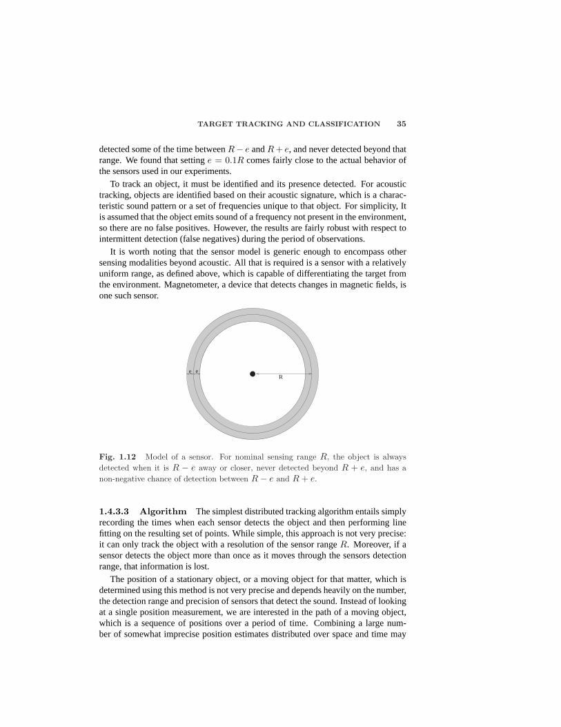
TARGET TRACKING AND CLASSIFICATION 35

detected some of the time betweenR− e andR + e, and never detected beyond thatrange. We found that settinge = 0.1R comes fairly close to the actual behavior ofthe sensors used in our experiments.

To track an object, it must be identified and its presence detected. For acoustictracking, objects are identified based on their acoustic signature, which is a charac-teristic sound pattern or a set of frequencies unique to that object. For simplicity, Itis assumed that the object emits sound of a frequency not present in the environment,so there are no false positives. However, the results are fairly robust with respect tointermittent detection (false negatives) during the period of observations.

It is worth noting that the sensor model is generic enough to encompass othersensing modalities beyond acoustic. All that is required is a sensor with a relativelyuniform range, as defined above, which is capable of differentiating the target fromthe environment. Magnetometer, a device that detects changes in magnetic fields, isone such sensor.

Ree

Fig. 1.12 Model of a sensor. For nominal sensing range R, the object is alwaysdetected when it is R − e away or closer, never detected beyond R + e, and has anon-negative chance of detection between R− e and R + e.

1.4.3.3 Algorithm The simplest distributed tracking algorithm entails simplyrecording the times when each sensor detects the object and then performing linefitting on the resulting set of points. While simple, this approach is not very precise:it can only track the object with a resolution of the sensor rangeR. Moreover, if asensor detects the object more than once as it moves through the sensors detectionrange, that information is lost.

The position of a stationary object, or a moving object for that matter, which isdetermined using this method is not very precise and depends heavily on the number,the detection range and precision of sensors that detect the sound. Instead of lookingat a single position measurement, we are interested in the path of a moving object,which is a sequence of positions over a period of time. Combining a large num-ber of somewhat imprecise position estimates distributed over space and time may

36

yield surprisingly accurate results. Cooperative tracking addresses the problem ofhigh-resolution tracking using sensor networks. It improves accuracy by combininginformation from neighboring sensors. The only requirement for cooperative track-ing to be used is that the density of sensor nodes must be high enough for the sensingranges of several sensors to overlap. When the object of interest enters the regionwhere multiple sensors can detect it, its position can be pinned down with a higherdegree of accuracy, since the intersection area is smaller than the detection area of asingle node. The outline of a generic cooperative tracking algorithm is as follows:

• Each node records the duration for which the object is in its range.

• Neighboring nodes exchange these times and their locations.

• For each point in time, the objects estimated position is computed as a weightedaverage of the detecting nodes locations.

• A line fitting algorithm is run on the resulting set of points.

Several of these steps require careful consideration. First, the algorithm implicitlyassumes that the nodes clocks are synchronized, and that the nodes know their loca-tions. Second, we obtain a position reading by a weighted average of the locations ofthe nodes that detected the sound at a given instant, but the exact weighting schemeis not specified. This is an important issue, as selecting an appropriate scheme willimprove accuracy, while a poor choice might be detrimental to it.

The simplest choice is to assign equal weights to all sensors readings. This ef-fectively puts the estimate of the objects position at the centroid of the polygon withsensors acting as vertices. This is a safe choice, and intuitively it should be moreaccurate than non-cooperative tracking. However it is possible to do even better.Consider Figure 1.13: sensors that are closer to the path of the target will stay in sen-sor range for a longer duration. Thus to increase accuracy, the weight of a sensorsreading should be proportional to some function of the duration for which the targethas been in range of that sensor.

Once the individual position estimates are computed, the final step of the line fit-ting algorithm can begin. Least squares regression can be used to find the equationof the line. It is interesting to note that the duration-based weighting scheme for po-sition estimates moves the points closer to the actual path, thus reducing variance inthe least squares computation. Also important is the fact that the multi-step approachenables early estimates of the path to be computed, so that continuous refinement ispossible as more data points become available. The resulting equation of the lineextrapolates the path of the object until it changes course sharply. This informationmay be used by the system, e.g. for asynchronous wake up of nodes likely to be inits path.

1.4.3.4 Data Aggregation The final step of the algorithm involves perform-ing a line fitting computation on the set of all the position estimates (or some sub-set of them). Unlike position estimates, which can be performed in a distributed

TARGET TRACKING AND CLASSIFICATION 37

R

d

r

R

d

r

Fig. 1.13 If the object’s speed is constant, detection time is directly proportionalto path segment d and inversely proportional to distance r from the sensor to object’strajectory.

manner with only local communication, this necessitates collecting sensor readingsfrom many sensor nodes at a centralized location for processing. This process iscalleddata aggregation, and it is present in one form or another in virtually all sen-sor network applications. The main concerns for data aggregation are timelinessand resource usage. Timeliness, with respect to sensor data, is critical to real-timemonitoring and control applications where stale data is useless or even detrimental.Resources, in particular network bandwidth and message buffers, are quite scarce innetworked embedded systems. Low bandwidth of small wireless transmitters andthe potential for contention with other messages drastically limit the amount of datathat can pass through the network.

We assume that some nodes in the sensor network are gateways nodes connectedto outside networks such as the Internet. To process the data from the sensor net-work, it needs to be sent through one of these gateway nodes to the more powerfulcomputers connected to the outside network. To do this efficiently, a tree rooted ateach gateway is constructed and spanning the entire network. Each sensor node inthe tree collects data from its children and sends it up the tree to either the closest orthe least busy gateway. This scheme addresses the conflicting requirements of lowbandwidth usage and timeliness of data: a near-shortest path is always taken, unlessits links are overloaded. What mentioned above is practical only if the outside net-work is low latency and high bandwidth, so it does not matter to which gateway thedata is sent.

1.4.4 Distributed Prediction Tracking (DPT)

The Distributed Prediction Tracking (DPT) algorithm is specifically aimed at ad-dressing the various challenges outlined in the Section 1.4 while accurately trackingmoving targets. As the name suggests, this algorithm does not require any centralcontrol point, eliminating the possibility of a single point of failure and making it ro-bust against random node failures. The tracking task is carried out distributively bysequentially involving the sensors located along the track of the moving target. DPT

38

assumes a cluster based architecture for the sensor network and the choice was mo-tivated by the need to ensure the sensor networks scalability and energy efficiency.Any suitable clustering mechanism from those proposed in literature may be usedand note that DPT does not impose any specific requirements or restrictions on thechoice of the clustering algorithm.

1.4.4.1 Assumptions of the DPT Algorithm While no assumption ismade on the choice of the clustering algorithm, we assume that the Cluster Head(CH) has the following information about all sensors belonging to its cluster: (1)Sensor identity, (2) Location and (3) Energy level. When tracking a moving targetand deciding which sensors to use for tracking, the cluster heads decision-makingprocedure will be based on this information. The assumptions about the sensorsare enumerated below. These assumptions are realistic and targeted at reducing theenergy cost and prolonging the whole networks lifetime as well.

1. All sensors have the same characteristics.

2. Sensors are randomly distributed across the whole sensing area with uniformdensity.

3. Each sensor has two sensing radii, normal beamr and high beamR. Thedefault operation uses the low beam and the high beam is turned on only whennecessary. The following relationship holds between the energy consumed bythe low and high beams:

Elowbeam

Ehighbeam=

r2

R2(1.2)

4. A sensors communication and sensing channel stay in the hibernation modemost of the time where they consume minimal energy. The communicationchannel will wake up routinely to receive possible messages from its clusterhead. The sensor will perform sensing according to its cluster heads require-ments.

In order to produce accurate enough information to locate the moving target, DPTrequires that at any given time there should be at least3 sensors to sense the targetjointly. The number3 is chosen as the compromise between increasing accuracyand minimizing the consumed energy (note that this is not a hard assumption anddepending on the sensor node specifications the number may vary).

No specific assumptions are made about the movement pattern of the targets.However, DPT assumes that the targets originate outside the sensing region and thenmove inside. Also, it is assumed that the movement of each tracked target needs tobe forwarded to a central location which we term the sink. In reality, the sink couldbe either a special node or a terminal associated with a human.

TARGET TRACKING AND CLASSIFICATION 39

1.4.4.2 DPT Algorithm The DPT algorithm comes into play after sensorsare deployed and clusters are formed. DPT distinguishes between theborder sensors,sensors located within a given distance of the border, andnon border sensorsinterms of their operation. While border sensors are required to keep sensing all timesin order to detect all targets that enter the sensing region, the non-border sensorssensing channel hibernates unless it is specifically asked to sense by its cluster head.Since the target is assumed to move from outside into the sensing area, it will bedetected by the border sensors when trespassing the border. As soon as a target isdetected, a sequence of tasks in the order ofsense-predict-communicate-sensearecarried out distributively by a series of sensors that are located along the targetstrack. This forms the essential idea behind the DPT algorithm.

Let CH1,CH2,...,CHN denote the sequence of cluster heads that become in-volved with tracking the targets as it proceeds from its very first location to the last.The information gathered by each cluster head is sent all the way back to the sink(either sent intact or after being aggregated) for further processing as well as to thedownstream cluster headCHi+1. TheTarget Identityis created when the target isfirst detected. This identity is unique and all cluster heads that co-track this targetuse it to identify the Target. In order to facilitate the smooth tracking of the target,CHi predicts the future location of the moving target, and informs the downstreamcluster headCHi+1 ahead of time about this target. The accuracy of thepredic-tion is very important if downstream cluster heads are to be identified accurately andthe overall tracking mechanism is to be effective. Many prediction mechanisms arepossible, the simplest one is a linear predictor, which only uses the previous twolocations to linearly predict the third location. Higher order prediction can also beadopt, which predicts thenth location information based on previousn − 1 actuallocations. Higher order prediction results in more accurate results, though, at thecost of greater energy consumption.

Sensor Selection Algorithm:After cluster headCHi predicts the location of thetarget, the downstream cluster headCHi+1 towards which the target is headed re-ceives a message fromCHi indicating this predicted location. With informationof all sensors belonging toCHi+1 available in its database, the search algorithmrunning atCHi+1 is able to locally decide the sensor-triplet to sense the target. Theselection rule chooses3 sensors (if possible) such that their distances to the predictedlocation are not only less than the sensors normal beamr, but also the smallest. Af-ter the sensor triplet is chosen,CHi+1 sends them awake-upmessage so that theyare ready to sense the target. If the prediction and selections process succeeds, aftersensing, each sensor will send a location message toCHi+1. If CHi+1 in unable tofind enough sensors eligible for this sensing task with the normal sensing beam, itwill try to search for eligible sensors within a distanceR, the higher sensing beam,from the predicted location. The selected sensors, whose distance from the predictedlocation is greater thanr and lower thanR, will now be contacted and instructed tosense with their high beam, while the rest of the sensors in the triplet use their normalbeam. IfCHi+1 is unable to find enough sensors even with high sensing beams, itasks its neighboring cluster heads for help.

40

Failure Recovery:Let’s first identify two possible failure scenarios. As describedin the previous subsections, each upstream cluster head sends a message to the ex-pected downstream cluster head. If the upstream cluster head does not get any con-firmation from the downstream cluster head after a given period of time, then it as-sumes that the downstream cluster head is no longer available and the target has beenlost. Another failure scenario occurs when the target changes it direction or speedso abruptly that it moves significantly away from the predicted location and falls outof the detectable region of the sensor-triplet selected for the sensing task. In both ofthese failure scenarios a straight forward solution is to wake up all sensors within agiven area, which is calculated based on the target’s previous actual location. There-captureradiusσ is an important parameter in this process and is decided by thetarget’s moving speed and time elapsed since it was last sensed.

1.5 EXPERIMENTAL LOCATION AND TRACKINGSYSTEMS

In this section, several location systems are introduced. Although they may not bespecially designed for wireless sensor networks, these design concepts and experi-ences will benefit future implementations of positioning systems in wireless sensornetworks.

1.5.1 Active Badge and Bat

1.5.1.1 Introduction Efficient location and coordination of staff in any largeorganization is a difficult and recurring problem. Hospitals, for example, may requireup-to-date information about the location of staff and patients, particularly whenmedical emergencies arise. In an office building, a receptionist is usually respon-sible for determining the location of staff members; in some organizations, publicaddress systems are provided to help a receptionist locate employees but, more fre-quently, a telephone is used to contact all the possible locations at which the requiredperson might be found. These solutions can cause a great deal of irritation and dis-ruption to other employees; a solution that provides direct location information ismore desirable. See [38] for detail information.

1.5.1.2 Active Badge vs Pager The conventional solution used for person-nel location is thepager system. In order to locate someone, a signal is sent out bya central facility that addresses a particular receiver unit (beeper) and produces anaudible signal. In addition, it may display a number to which the called party shouldphone back.(Some systems allow a vocal message to be conveyed about the call-back number.) It is then up to the recipient to use the conventional telephone systemto call back confirming the signal and to determine the required action. Althoughuseful, in practice there are still circumstances where it is not ideal. For instance, ifthe called party does not reply, the controller has no idea whether they are in an area

EXPERIMENTAL LOCATION AND TRACKING SYSTEMS 41

where the signal does not penetrate, have been completely out of the area for sometime, have been too busy to reply, or have misheard or misread the call-back number.Moreover, in the case where there are a number of people who could respond to acrisis situation, it is not known which one is the nearest to the crisis and therefore themost suitable to contact. An alternative approach is totag a person and try to locatethe tag. The main application of personal tags has been in the area of access controland logging [15]. In many high-security installations, card-key systems restrict ac-cess to various parts of the installation. If there are enough access-control zones, thesame mechanism can also provide location information on a per-zone basis. For thiskind of system, the information is positive and directly available to be acted upon.However, it is inappropriate for most organizations to use access-control techniquesto derive location information because of the inconvenience experienced by person-nel. There are additional problems arising from groups of people obtaining access toadjoining zones with only one card-key, which is a hard problem to solve.

1.5.1.3 An Active Badge Design A solution to the problem of automati-cally determining the location of an individual has been to design a tag in the formof an ’Active Badge’ that emits a unique code for approximately a tenth of a secondevery 15 seconds (a beacon). These periodic signals are picked up by a networkof sensors placed around the host building. A master station, also connected to thenetwork, polls the sensors for badge ’sightings’, processes the data, and then makesit available to clients that may display it in a useful visual form. The badge wasdesigned in a package roughly 55x55x7mm and weighs a comfortable 40g. Pulse-width modulated infrared (IR) signals are used for signaling between the badge andsensor [31] mainly because: IR solid-state emitters and detectors can be made verysmall and very cheaply (unlike ultrasonic transducers); they can be made to oper-ate with a 6m range, and the signals are reflected by partitions and therefore are notdirectional when used inside a small room. Moreover, the signals will not travelthrough walls, unlike radio signals that can penetrate the partitions found in officebuildings. Infrared communication has been used in a number of commercial appli-cations ranging from the remote control of domestic appliances to data backup linksfor programmable calculators and personal organizers [12]. More recently, IR hasbeen used as the basis for wireless local area networks [27]. Because IR technol-ogy has already been exploited commercially, it is inexpensive and readily availablefor developing new applications such as the Active Badge. An active signaling unitconsumes power; therefore, the signaling rate is an important design issue. Firstly,by only emitting a signal every 15 seconds, the mean current consumption can bevery small with the result that ’badge-sized’ batteries will last for about one year.Secondly, it is a requirement that several people in the same locality be detectableby the system. Because the signals have a duration of only one-tenth of a second,there is approximately a 2/150 chance that two signals will collide when two badgesare placed in the same location. For a small number of people, there is a goodprobability they will all be detected. Even so, in order to improve this chance, thebeacon oscillator has been deliberately designed around low-tolerance components.The components used for the beacon oscillator have a 10% tolerance rating; for two

42

badges to remain in synchronization for even a single 15-second beacon period, thecomponents would have to be matched better than 1.4%. It is very likely that twobadges, which at some instant may be synchronized, will have slightly differing fre-quencies and thus lose synchronization within a few beacon periods. In practice,synchronization has not been a problem. The Active Badge also incorporates a light-dependent component that, when dark, turns the badge off to conserve battery life.Reduced lighting also increases the period of the beacon signal to a time greater than15 seconds. In ambient lighting conditions in a room, this effect only slightly modi-fies the period, but it is another factor that ensures synchronized badges will not staysynchronized very long. If the badge is placed in a drawer out of office hours, atweekends and during vacation, the effective lifetime of the batteries is increased bya factor of 4. Note that the more obvious solution of a manual switch was considereda bad idea as it was likely that a badge user would forget to turn it on. Other optionsfor switching the device on included a tilt switch and an accelerometer, although thesize limitation of a badge precluded using them in the initial experimental system. Adisadvantage of an infrequent signal from the badge is that the location of a badgeis only known, at best, to a 15-second time window. However, because in generala person tends to move relatively slowly in an office building, the information theActive Badge system provides is very accurate. An Active Badge signal is transmit-ted to a sensor through an optical path. This path may be found indirectly through asurface reflection, for example, from a wall. A badge must be worn on the outsideof clothing, so an essential part of the badge case design was the clip allowing it tobe easily attached to a shirt or a blouse. Most commonly, the badge was worn at thebreast pocket position; however, some people preferred a belt or waist position. Thebelt position was not as good when the wearer was seated at a desk but typically thesystem still detected enough signals to locate the badge.

Active Badge location system developed at Olivetti Research Laboratory and nowAT&T at Cambridge.

1.5.1.4 Bat System A successor of the Active Badge system is the Bat sys-tem [4], which consists of a collection of wireless transmitters, a matrix of receiverelements, and a central RF base station. The wireless transmitters, called bats, can becarried by a tagged object and/or attached to equipment. The sensor system measuresthe time of flight of the ultrasonic pulses emitted from a bat to receivers installed inknown and fixed positions. It uses the time difference to estimate the position ofeach bat by trilateration. The RF base station coordinates the activity of bats byperiodically broadcasting messages to them. Upon hearing a message, a bat sendsout an ultrasonic pulse. A receiver that receives the initial RF signal from the basestation determines the time interval between receipt of the RF signal and receiptof the corresponding ultrasonic signal. It then estimates its distance from the bat.These distances are sent to the computer, which performs data analysis. By collect-ing enough distance readings, it can determine the location of the bat within 3 cm oferror in a three-dimensional space at 95% accuracy. This accuracy is quite enoughfor most location-aware services; however, the deployment cost is high.

EXPERIMENTAL LOCATION AND TRACKING SYSTEMS 43

1.5.2 Cricket

1.5.2.1 Introduction The design and deployment of a system for obtaininglocation and spatial information in an indoor environment is a challenging task forseveral reasons, including the preservation of user privacy, administration and man-agement overheads, system scalability, and the harsh nature of indoor wireless chan-nels. The degree of privacy offered by the system is an important deployment consid-eration, since people often value their privacy highly. The administrative overheadto manage and maintain the hardware and software infrastructure must be minimalbecause of the potentially large number (possibly several thousands in a building) ofdevices and networked services that would be part of the system, and the communi-cation protocols must be able to scale to a high spatial density of devices. Finally,indoor environments often contain substantial amounts of metal and other such re-flective materials that affect the propagation of radio frequency (RF) signals in non-trivial ways, causing severe multipath effects, dead-spots, noise, and interference.See [29] for more information about Cricket.

Cricket is a location-support system for in-building, mobile, location-dependentapplications. It allows applications running on mobile and static nodes to learn theirphysical location by using listeners that hear and analyze information from beaconsspread throughout the building. Cricket is the result of several design goals, includ-ing user privacy, decentralized administration, network heterogeneity, and low cost.Rather than explicitly tracking user location, Cricket helps devices learn where theyare and lets them decide whom to advertise this information to; it does not rely onany centralized management or control and there is no explicit coordination betweenbeacons; it provides information to devices regardless of their type of network con-nectivity; and each Cricket device is made from off-the-shelf components and costsless than U.S. $10.

By not tracking users and services, user privacy concerns are adequately met.We emphasize that Cricket is alocation-supportsystem, rather than a conventionallocation trackingsystem that tracks and stores location information for services andusers in a centrally maintained database.

The design of Cricket was driven by the following specific goals:

• User privacy: Whenever a system for providing location information to clientshas been deployed in the past, the issue of user privacy has arisen. This isbecause many previous systems were location tracking systems, where a data-base kept track of the locations of all the entities, including users in the system.To address this concern, we designed a location support system, which allowsclients to learn their location without centralized tracking in order to constructlocation-specific queries for resources.

• Decentralized administration: Our goal is widespread building-wide de-ployment. We believe that it is not possible to deploy and administer a systemin a scalable way when all control and management functions are centralized.Our design is decentralized - the ”owner” of a space in a building (e.g.,the

44

occupant of a room) configures and installs a location beacon that announcesthe identity of that space (some character string) and each beacon seamlesslyintegrates with the rest of the system. Location receiver hardware, called alistener, is attached to every device of interest to a user. Listeners use an in-ference algorithm to determine the space in which they are currently locatedby listening to beacon announcements. And there is no need to keep track ofindividual components within the system.

• Network heterogeneity:A wide variety of network technologies exist in mostbuilding environments. In our own laboratory, devices and users connectedover 10/100 Mbps Ethernet, three different types of indoor wireless LANs,cellular digital packet data (CDPD), infrared, public telephone, and power lineusing X10 [1]. Independent of which technology they use to serve or gainaccess to information, many services and clients can benefit from learningtheir location in an automatic way, and we would like to accommodate them.In our design, we achieve this by decoupling the Cricket system from otherdata communication mechanisms.

• Cost: Achieving building-wide deployment requires cost effective compo-nents.We use commercial, off-the-shelf, inexpensive components in Cricket,setting and meeting the goal of less than U.S. $10 per location beacon andlistener. Our design involves no custom hardware and is small enough to fit inone’s palm.

• Room-sized granularity: Our goal is a system where spatial regions can bedetermined to within a few square feet, so as to distinguish portions of rooms.This requires the ability to demarcate and determine boundaries between re-gions corresponding to different beacons.

Cricket uses a combination of RF and ultrasound to provide a location-supportservice to users and applications. Wall- and ceiling-mounted beacons are spreadthrough the building, publishing location information on an RF signal. With eachRF advertisement, the beacon transmits a concurrent ultrasonic pulse. The listen-ers receive these RF and ultrasonic signals, correlate them to each other, and inferthe space they are currently in. The beacons use a decentralized randomized trans-mission algorithm to minimize collisions and interference amongst each other. Thelisteners implement a decoding algorithm to overcome the effects of ultrasound mul-tipath and RF interference.

1.5.2.2 System Architecture The only configuration required in Cricket issetting the string for a space that is disseminated by a beacon. The specific string isa function of the resource discovery protocol being used, and Cricket allows any oneof several possibilities (in Section 5 we describe our implementation platform andintegration with INS). Cricket also provides a way by which the owner of a roomcan securely set and change the space identifier that is sent in the advertisements.This is done by sending a special message over the same RF channel that is used for

EXPERIMENTAL LOCATION AND TRACKING SYSTEMS 45

the advertisements, after authenticating the user via a password. At this stage, wehave chosen to allow this change only from within physical proximity of the room orlocation where the beacon is located. This makes the system somewhat more securethan if we allowed this to be done from afar. The boundaries between adjacentspaces can either be real, as in a wall separating two rooms, or virtual, as in a non-physical partition used to separate portions of a room. The precision of the systemis determined by how well the listener can detect the boundary between two spaces,while the granularity of the system is the smallest possible size for a geographic spacesuch that boundaries can be detected with a high degree of precision. A third metric,accuracy is used to calibrate individual beacons and listeners; it is the degree towhich the distance from a beacon, estimated by a listener, matches the true distance.While our experiments show that the distance accuracy of our hardware is smallerthan a few inches, what matters is the precision and granularity of the system. Thesedepend on the algorithms and the placement of beacons across boundaries. Our goalis a system with a close-to-100of a few feet (a portion of a room).

1.5.2.3 Beacon positioning and configuration The positioning of a bea-con within a room or space plays a nontrivial role in enabling listeners to make thecorrect choice of their location. For example, consider the positioning shown in Fig-ure 2. Although the receiver is in Room A, the listener finds the beacon in Room B tobe closer and will end up using the space identifier advertised by the latter. One wayof overcoming this is to maintain a centralized repository of the physical locationsof each beacon and provide this data to listeners. Systems like the Bat essentiallyuse this type of approach, where the central controller knows where each wall- orceiling-mounted device is located, but it suffers from two problems that make it un-suitable for us. First, user-privacy is compromised because a listener now needs tomake active contact to learn where it is (observe that in Cricket, a listener is com-pletely passive). Second, it requires a centrally managed service, which does notsuit our autonomously managed environment particularly well. Fortunately, there isa simple engineering solution to this problem that preserves privacy and is decen-tralized. Whenever a beacon is placed to demarcate a physical or virtual boundarycorresponding to a different space, it must be placed at a fixed distance away fromthe boundary demarcating the two spaces. Figure 3 shows an example of this in asetting with both real and virtual boundaries. Such placement ensures that a listenerrarely makes a wrong choice, unless caught within a small distance (1 foot in our cur-rent implementation) from the boundary between two beacons advertising differentspaces. In this case, it is often equally valid to pick either beacon as the closest.

1.5.3 RADAR:An In-Building RF-based User Location andTracking System and Nibble

RADAR [8] is a radio-frequency (RF) based system for locating and tracking usersinside buildings. RADAR operates by recording and processing signal strength in-formation at multiple base stations positioned to provide overlapping coverage in

46

the area of interest. It combines empirical measurements with signal propagationmodeling to determine user location and thereby enable location-aware services andapplications.

RADAR complements the data networking capabilities of RF wireless LANs withaccurate user location and tracking capabilities, thereby enhancing the value of suchnetworks. RADAR uses signal strength information gathered at multiple receiverlocations to triangulate the user’s coordinates. Triangulation is done using bothempirically-determined and theoretically-computed signal strength information.

Recently, several location systems have been proposed for wide-area cellular sys-tems [35]. The technological alternatives for locating cellular telephones involvemeasuring the signal attenuation, the angle of arrival (AOA), and/ or the time dif-ference of arrival (TDOA). While these systems have been found to be promising inoutdoor environments, their effectiveness in indoor environments is limited by themultiple reflections suffered by the RF signal, and the inability of off-the-shelf andinexpensive hardware to provide fine-grain time synchronization.

Systems based on the Global Positioning System [28], while very useful outdoors,are ineffective indoors because buildings block GPS transmissions. RADAR differsfrom previous work in that it tackles the problem of user location and tracking on awidely available radio frequency based wireless network in an in-building environ-ment. RF networks offer a significant advantage over IR (Infra Red) networks interms of range, scalability, deployment, and maintenance. With speeds of up to 11Mbps, these systems have gained rapid acceptance and are being widely deployed inoffices, schools, homes, etc.

RADAR has been developed by a Microsoft Research group. It is a building-widetracking system based on the IEEE 802.11 WaveLAN wireless networking technol-ogy [8]. RADAR measures, at the base station, the signal strength and signal-to-noise ratio of signals that wireless devices send, then it uses this data to computethe 2D position within a building. Microsoft has developed two RADAR imple-mentations: one using scene analysis and the other using lateration. The RADARapproach offers two advantages: It requires only a few base stations, and it uses thesame infrastructure that provides the buildings general-purpose wireless networking.Likewise, RADAR suffers two disadvantages. First, the object it is tracking mustsupport a wireless LAN, which may be impractical on small or power-constraineddevices. Second, generalizing RADAR to multi-floored buildings or three dimen-sions presents a nontrivial problem. RADARs scene-analysis implementation canplace objects to within about 3 meters of their actual position with50 percent prob-ability, while the signal-strength lateration implementation has4.3-meter accuracyat the same probability level. Although the scene-analysis version provides greateraccuracy, significant changes in the environment, such as moving metal file cabi-nets or large groups of people congregating in rooms or hallways, may necessitatereconstructing the predefined signal-strength database or creating an entirely newdatabase.

Several commercial companies such as WhereNet [2] and Pinpoint [3] sell wire-less asset-tracking packages, which are similar in form to RADAR. Pinpoints 3D-iD

EXPERIMENTAL LOCATION AND TRACKING SYSTEMS 47

performs indoor position tracking using proprietary base station and tag hardwareto measure radio time of flight. Pinpoints system achieves 1- to 3-meter accuracyand, by virtue of being a commercial product, offers easier deployment and admin-istration than many research systems. The 3D-iD system suffers the disadvantagethat each antenna has a narrow cone of influence, which can make ubiquitous de-ployment prohibitively expensive. Thus, 3D-iD best suits large indoor space settingssuch as hospitals or warehouses. It has difficulty interoperating with the 802.11 wire-less networking infrastructure because of radio spectrum collision in the unregulatedIndustrial, Scientific, and Medical (ISM) band.

The Nibble also adopts the IEEE 802.11 infrastructure for positioning purpose.Nibble uses the probability-based approach in Subsection 1.2.2.2. It relies on a fusionservice to infer the location of an object from measured signal strengths. Data arecharacterized probabilistically and input into the fusion service. The output of thefusion service is a probability distribution over a random variable that representssome context.

1.5.4 CSIE/NCTU Indoor Tour Guide

The prototype indoor tour guide system has been developed at the Department ofComputer Science and Information Engineering, National Chiao Tung University(CSIE/NCTU), Taiwan. The hardware platforms of this project include several Com-paq iPAQ PDAs and laptops. Each mobile station is equipped with a Lucent OrinocoGold wireless card. Signal strengths are used for indoor positioning. The probability-based pattern-matching algorithm in Subsection 1.2.2.2 is used.

There is a manager or control center responsible for monitoring each users move-ments, configuring the system, and planning logical areas and events. The locationserver takes care of the location discovery job and the service server is in charge ofmessage delivery. The database can record users profiles; the gateway can conductlocation-based access control to the Internet. One of the innovations in this projectis that an event-driven messaging system has been designed. A short message can bedelivered to a user when he enters or leaves a logical area. The event-driven messagecan also be triggered by a combination of time, location, and property of location(such as who is in the location and when the location is reserved for meetings). Auser can set up a message and a corresponding event to trigger the delivery of themessage. The manager will check the event list periodically and initiate messages,when necessary, with the service server. Messages can be unicast or broadcast. Theexpectation is that streaming multimedia can be delivered in the next stage. The sys-tem can also be applied to support a smart library. Another innovation is to providelocation-based access control. In certain rooms, such as classrooms and meetingrooms, users may be prohibited from accessing certain sensitive Web pages. Theserules can be organized through the manager and set up at the gateway.

48

1.6 CONCLUSION

In this chapter, some fundamental techniques in positioning and location trackinghave been discussed and several experimental systems reviewed. Location infor-mation may enable new types of services. Accuracy and deployment costs are twofactors that may contradict each other, but both are important factors for the successof location-based services.

References

1. X-10 home page: http://www.x10.com/homepage.htm.

2. Widata home page: http://www.widata.com/.

3. Pinpoint home page: http://www.rftechnologies.com/pinpoint/.

4. Mike Addlesee, Rupert Curwen, Steve Hodges, Joe Newman, Pete Steggles,Andy Ward, and Andy Hopper. Implementing a sentient computing system.Computer, 34(8):50–56, 2001.

5. Localization James Aspnes. On the computational complexity of sensor net-work.

6. S. Atiya and G.Hager. Real-time vision-based robot localization. pages 785–800, 1993. IEEE Trans. Robot. Automat. 9 (6).

7. P. Bahl, A. Balachandran, and V. Padmanabhan. Enhancements to the radar userlocation and tracking system, 2000.

8. Paramvir Bahl and Venkata N. Padmanabhan. RADAR: An in-building RF-based user location and tracking system. InINFOCOM (2), pages 775–784,2000.

9. P. Bose, P. Morin, I. Stojmenovic, and J. Urrutia. Routing with guaranteed de-livery in ad hoc wireless networks.ACM/Kluwer Wireless Networks, 7(6):609–616, 2001. 3rd int. Workshop on Discrete Algorithms and methods for mobilecomputing and communications, 1999, 48-55.

10. N. Bulusu, J. Heidemann, and D. Estrin. Gps-less low cost outdoor localizationfor very small devices, 2000.

11. Srdan Capkun, Maher Hamdi, and Jean-Pierre Hubaux. GPS-free positioning inmobile ad-hoc networks. InHICSS, 2001.

12. S. L. Harper, Worsley R. L., and B. A. Stephens. An infrared link for low-costcalculators and printers. InHewlett-Packard Journal, October 1987.

49

50 REFERENCES

13. Andy Harter, Andy Hopper, Pete Steggles, Andy Ward, and Paul Webster. Theanatomy of a context-aware application. InMobile Computing and Networking,pages 59–68, 1999.

14. J. Heidemann and N. Bulusu. Using geospatial information in sensor networks,2001.

15. P. Hewkin. Smart tags the distributed memory revolution. InIEEE Review, June1989.

16. Jeffrey Hightower and Gaetano Borriella. Location systems for ubiquitous com-puting. IEEE Computer, 34(8):57–66, 2001.

17. Jason Hill, Robert Szewczyk, Alec Woo, Seth Hollar, David E. Culler, andKristofer S. J. Pister. System architecture directions for networked sensors.In Architectural Support for Programming Languages and Operating Systems,pages 93–104, 2000.

18. Brad Karp and H.T. Kung. Gpsr: Greedy perimeter stateless routing for wire-less networks. InProc. of the ACM/IEEE International Conference on MobileComputing and Networking (MobiCom), 2000.

19. Y. Ko and N. Vaidya. Geocasting in mobile ad hoc networks: Location-basedmulticast algorithms, 1998.

20. Y. Ko and N. Vaidya. GeoTORA: A protocol for geocasting in mobile ad hocnetworks. Technical Report 00-010, Dept. of Computer Science, Texas A&MUniversity, March 2000.

21. Koen Langendoen and Niels Reijers. Distributed localization in wireless sensornetworks: a quantitative comparison.Comput. Networks, 43(4):499–518, 2003.

22. J. Leonard and H.Durrant-Whyte. Mobile robot localization by tracking geo-metric beacons. pages 376–382, 1991. IEEE Trans. Robot. Automat. 7 (3).

23. D. Li, K. Wong, Y. Hu, and A. Sayeed. Detection, classification, and tracking oftargets, 2002.

24. J. Li, J. Jannotti, D. De Couto, D. Karger, and R. Morris. A scalable locationservice for geographic ad-hoc routing. InProceedings of the 6th ACM Interna-tional Conference on Mobile Computing and Networking (MobiCom ’00), pages120–130, 2000.

25. Julio C. Navas and Tomasz Imielinski. GeoCast – geographic addressing androuting. InMobile Computing and Networking, pages 66–76, 1997.

26. Dragos Niculescu and Badri Nath. Ad hoc positioning system (APS). InGLOBECOM (1), pages 2926–2931, 2001.

REFERENCES 51

27. A. Paepcke, R.D. Crawford, R. Jamp, C. A. Freeman, and F.J. Lee. Chipnet: Anoptical network of terminals andworkstations. InElsevier Science Publishers B.V. (North-Holland), Computer and ISDN Systems 15, pages 203–215, 1988.

28. P.Eng and P.Mirsa. Special issue on global positioning system. InProceedingsof the IEEE, volume 87, pages 3–15, January 1999.

29. Nissanka B. Priyantha, Anit Chakraborty, and Hari Balakrishnan. The cricketlocation-support system. InMobile Computing and Networking, pages 32–43,2000.

30. T. Roos, P. Myllymaki, H. Tirri, P. Misikangas, and J. Sievanen. A probabilisticapproach to wlan user location estimation. InInt. J. Wireless Inf. Networks,2002.

31. Satellite, Cable, and TV IC Handbook. InPlessey Semiconductors, pages64,67,124, 1988.

32. C. Savarese, J. Rabay, and K. Langendoen. Robust positioning algorithms fordistributed ad-hoc wireless sensor networks usenix technical annual conference,2002.

33. A. Savvides, H. Park, and M. Srivastava. The bits and flops of the n-hop multi-lateration primitive for node localization problems, 2002.

34. Andreas Savvides, Chih-Chieh Han, and Mani B. Strivastava. Dynamic fine-grained localization in ad-hoc networks of sensors. InMobile Computing andNetworking, pages 166–179, 2001.

35. S. Tekinay. Wireless geolocation systems and services. InSpecial Issue of theIEEE Communications Magazine, April 1998.

36. R. Tins, L. Navarro-Serment, and C. Paredis. Fault tolerant localization of teamsof distributed robots, 2001.

37. Y.-C. Tseng, S.-P. Kuo, H.-W. Lee, and C.-F. Huang. Location tracking in awireless sensor network by mobile agents and its data fusion strategies. InInt.Workshop Inf. Process. Sensor Networks (IPSN), 2003.

38. Roy Want, Andy Hopper, Veronica Falcao, and Jonathan Gibbons. The activebadge location system. Technical Report 92.1, Olivetti Research Ltd. (ORL),24a Trumpington Street, Cambridge CB2 1QA, 1992.

39. M. Youssef, A. Agrawala, and U. Shankar. Wlan location determination viaclustering and probability distributions. InIEEE PerCom, 2003.