COST: A POSSIBLE EXPLANATION FOR RISK PREMIUM?

by

Zhihua Shen

A thesis submitted iri partial· fulfillment of the requirements for the degree

of

Master of Science

m

Applied Economics

MONTANA STATE UNIVERSITY Bozeman, Montana

September 1995

ii

APPROVAL

of a thesis submitted by

Zhihua Shen

This thesis has been read by each member of the thesis committee and has been mnd to be satisfactory regarding content, English usage, format, citations, bibliographic yle, and consistency, and is ready for submission to the College of Graduate Studies.

;o-r- rr ~k=z~,s?Q Chairpersoi?, Graduate Committee Date

Approved for the Major Department

.. \:~L 0 v

Head, Major Department Date

Approved for the College of Graduate Studies

Date Graduate Dean

iii

STATEMENT OF PERMISSION TO USE

In presenting this thesis in partial fulfillment of the requirements for a master's

iegree at Montana State University, I agree that the Library shall make it available to

Jorrowers under rules of the Library.

If I have indicated my intention to copyright this thesis by including a copyright notice

?age, copying is allowable only for scholarly purposes, consistent with "fair use" as prescribed

n the U.S. Copyright Law. Requests for permission for extended quotation from or

~eproduction of this thesis (paper) in whole or in part may be granted only by the copyright

1older.

~ignature

Date )g, 192~ I

iv

ACKNOWLEDGMENTS

I would like to gratefully acknowledge the patience and guidance of the chairman of

my graduate committee, Professor Myles J. Watts, who helped me not only during the

preparation of this thesis, but also throughout the course of my graduate work. I would also

like to acknowledge the instruction, encouragement, and assistance I received from my

other graduate committee members, Professors Dan Benjamin, Joe Atwood, and James Lin.

I would like to express my appreciation to my classmates - Dan, Mike, Pat and Hayley for

numerous valuable comments. I also thank our nice staff- Kathy, Tammy and Renee for

their kind assistance. Finally, I would like to express my gratitude to my parents TuAn

Shen & LaiFang Zhang, and my brother, Zhengxiang Fei, for their encouragement and

support.

v

TABLE OF CONTENTS

Page APPROVAL . . . . . . . . . . . . .. . . . . . . . . . . . . . . . . . . . . . . . . . . . . . . . . . . . . . . . . . . . . . u

STATEMENT OF PERMISSION TO USE . . . . . . . . . . . . . . . . . . . . . . . . . . . . . . . . . m

ACKNOWLEDGMENTS. . . . . . . . . . . . . . . . . . . . . . . . . . . . . . . . . . . . . . . . . . . . . . . iv

TABLE OF CONTENTS . . . . . . . . . . . . . . . . . . . . . . . . . . . . . . . . . . . . . . . . . . . . . . . v

LIST OF TABLES . . . . . . . . . . . .. . .. . . . . . . .. . . . . . . . . . . . . . . . . . . . . . . . . . . . . . vii

LIST OF FIGURES . . . . . . . . . . . . . . . . . . . . . . . . . . . . . . . . . . . . . . . . . . . . . . . . . . . . viii

ABSTRACT . . . . . . . . . . . . . . . . . . . . . . . . . . . . . . . . . . . . . . . . . . . . . . . . . . . . . . . . . . ix

1. INTRODUCTION . . . . . . . . . . . . . . . . . . . . . . . . . . . . . . . . . . . . . . . . . . . . . . . . . . . 1

Statement of the Problem .. :. . . . . . . . . . . . . . . . . . . . . . . . . . . . . . . . . . . . 1 Model Development .......................................... : . 3 Objective . . . . . . . . . . . . . . . . . . . . . . . . . . . . . . . . . . . . . . . . . . . . . . . . . . . . . 8 Outline of Thesis . . . . . . . . . . . . . . . . . . . . . . . . . . . . . . . . . . . . . . . . . . . . . . 9

2. LITERATURE REVIEW ... , . . . . . . . . . . . . . . . . . . . . . . . . . . . . . . . . . . . . . . . . . 10

Market Efficiency Theory. . . . . . . . . . . . . . . . . . . . . . . . . . . . . . . . . . . . . . . . 10 Option Pricing and Put-Call Parity Theory . . . . . . . . . . . . . . . . . . . . . . . . . 13 Risk Premium and the CAPM Model. .............................. 14 Random Walk Theory........................................... 18

3. THE MODEL . . . . . . . . . . . . . . . . . . . . . . . . . . . . . . . . . . . . . . . . . . . . . . . . . . . . . . 21

4. EXPECTED STOCK PRICE . . . . . . . . . . . . . . . . . . . . . . . . . . . . . . . . . . . . . . . . . . 27

Testing Random Walk . . . . . . . . . . . . . . . . . . . . . . . . . . . . . . . . . . . . . . . . . . 27 Four Methods of Estimating Stock Price . . . . . . . . . . . . . . . . . . . . . . . . . . . . 31

vi

TABLE OF CONTENTS -- Continued

5. DATA ............................................ 39

The First Data Set . . . . . . . . . . . . . . . . . . . . . . . . . . . . . . . . 39 The Second Data Set . . . . . . . . . . . . . . . . . . . . . . . . . . . . . . 39

6. EMPIRICAL FINDINGS ................................. 42

OLS Estimation . . . . . . . . . . . . . . . . . . . . . . . . . . . . . . . . . 42 Autocorrelation and Adjusted Estimation . . . . . . . . . . . . . . . . . . 50 Heteroskedasticity . . . . . . . . . . . . . . . . . . . . . . . . . . . . . . . . 54 Summary of Empirical Results . . . . . . . . . . . . . . . . . . . . . . . . 54

7. CONCLUSIONS AND REMARKS ........................... 56

REFERENCES CITED .................................... 5.8

APPENDICES. . ....................................... 63 Appendix A-- Notes .............................. 64

Appendix B -- Sample Data . . . . . . . . . . . . . . . . . . . . . . . . . . 70

vii

LIST OFT ABLES

Table Page

1. Rates of Return and Betas for Selected Companies (1945-1970) .......................... · .......... 17

2. Transaction Summaries for Portfolios 1 and 2 . . . . . . . . . . . . . . . . . . . . . . . . . . . 22

3. Summary of Four Estimation Methods Used to Estimate E(S') ..................................... ·. . . . . . . . 42

4. OLS Estimation of Coefficients in Equation (9), Using 935 Observations ...... , . . . . . . . . . . . . . . . . . . . . . . . . . . . . . . . . . . . . . 49

5. Statistics Summary of The Treasury Bill Rate, January- June, 1992 ............ ~ . . . . . . . . . . . . . . . . . . . . . . . . . . . . . . . . . . 49

6. OLS Estimation of Coefficients in Equation (9), Using Cross-sectional Time-Series Data (874 Observations). . . . . . . . . . . . . . . 52

7. Adjusted Estimation of Coefficients in Equation ( 18), · Using Cross-sectional Time-Series Data (874 Observations) .... : . . . . . . . . . . 53

8. Comparison of Risk Premium Estimated by Proposed Model And by the CAPM Model.. ............... ~ . . . . . . . . . 56

9. Composition of Annual Returns of PCP Based on Thesis Data . . . . . . . . . . . . . . . . . . . . . . . . . . . . . . . . . . . . . . . . . . . . . 67

viii

LIST OF FIGURES

Figure Page

1. Risk Premium Estimation in this Thesis and in the CAPM Model . . . . . . . . . . . . . . . . .. . . . . . . . . . . . . . . . . . . . . . . . . 8

2. Optimal Portfolio Choice for a Risk averse Investor and an Efficient Set ............................. 15

3. Decomposition of Returns - Dividends & Appreciation J an-J un 1992 . . . . . . . . . . . . . . . . . . . . . . . . . . . . . . . . . . . . . . 23

4. Dividend of S&P 500 Stock - Annual Quarterly Dividend, Dec 1991 .............. 24

5. S&P 500 Market Prices -January- June, 1992, In Nominal Terms ............................. 28

6. Random Walk- S&P 500 Returns In Real Terms 1941-1991 ............... 30

7. S&P 500 Prices 1940-1991 In Nominal Terms ........................... 32

8. S&P 500 Prices 1940-1991, Inflated Adjusted ........................... 33

9. Actual vs Expected Inflation·(1942-1991) .............................. 36

10. Plot of R1 Against N- In Real Terms, 935 Observations. . . . . . . . . . . . . . . . . . 44

11. Plot of R2 Against N - Method 1. . . . . . . . . . . . . . . . . . . . . . . . . . . . . . . . . . . . . 45

12. Plot ofR2 Against N- Method 2 ..................................... 46

13. Plot of R2 Against N- Method 3. . . . . . . . . . . . . . . . . . . . . . . . . . . . . . . . . . . . . 47

14. Plot ofR2 Against N- Method 4 ..................................... 48

ix

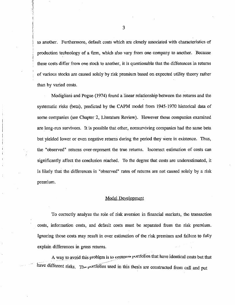
ABSTRACT

Transaction costs, information costs and defaults costs are suspected to partially explain differences in returns which were previously attributed to risk premiums in the financial markets. Two portfolios with identical costs are constructed from a Put, a Call, and underlying S&P 500 stocks, with the first Portfolio being hedged (Put-Call Parity) and the second Portfolio being unhedged (with systematic beta close to 2). The expected stock prices of S&P 500 were calculated based on 52-year historical data using several methods, and returns of the two portfolios were obtained and compared, using 935 observations of S&P 500 from January 2, 1992 through June 30, 1992. A linear regression model adjusted for cross-sectional heteroskedasticity and auto-correlation was used to estimate the expected risk premium rate.

Transaction, information and default costs were statistically significant and estimated at 0.6% of value annually. These costs reduce the risk premium estimated by the Capital Asset Pricing Model.

1

CHAPTER 1

INTRODUCTION

Statement of the Problem

Since the Capital Asset Pricing Model (CAPM) and the Arbitrage Pricing Theory

(APT) were developed by Sharpe,. Ross, and other economists in the 1960s, the subject of

risk premium has been widely studied in finance. Standard financial theory states that more

risky assets generate higher average rates of return and that there exists a market price for

risk, identified as "risk premium" (defined as systematic risk or beta in this paper).

However factors other than risk premium may explain differences in returns across

risky assets. One possible explanation is the costs involved in buying and selling stocks.

Several costs are incurred by investing in financial markets: transaction costs, information

costs, and default costs. Transaction costs include brokerage fees, bid-ask spreads, the seat

price in the New York Stock Exchange (NYSE) or the American Stock Exchange (AMEX),

and taxes. Information costs include time, money spent in searching for the stock and price,

data collecting costs, analyzing fees, and human capital costs, some of which are

nonmonetary. Finally, every company has a risk of going bankrupt. When default occurs,

the stockholders of that company may lose their investments. Those losses are defined as

default costs.

2

For example, banks usually charge higher interest rates to those borrowers with higher

possibility of default (Benjamin, 1978). While this can be explained by the risk premium

theory, it also can be explained by the costs associated with default. Default usually results

in banks sustaining losses. Thus banks must charge a higher contractual interest rate to

recoup those losses (Watts, etc., 1992).

Some of those costs are explicit (e.g., taxes), while others are implicit, such as time

consumed in searching for the best price. Some costs are proportional percentages, or

directly related with each transaction, such as commission fee, while some are fixed, such as

the seat price of the NYSE. The complexity of costs makes estimation difficult.

As discussed in the literature, as well as in this thesis (see Chapter 6), the returns from

the Put-Call Parity (PCP), which is free from risk, are consistently and significantly greater

than the most obvious opportunity cost--riskless interest rate--implying that costs such as

transaction costs, information costs, and default costs exist in the financial markets. In most

of the previous research, however, the yields from an asset are calculated by summing the

market price appreciation and the accumulated dividends. Such an approach ignores

differences in the costs earlier discussed, thereby influencing the comparison of returns

across different stocks.

For example, a broker may charge a higher commission for trading rare, low-volume

stocks, and a lower commission for trading prominent and frequently-traded stocks. It is

much easier to collect information regarding performances and prospects of those

companies that are large and well known than for the small, local, or marginal companies.

The information costs associated with stocks are therefore not identical from one company

3

to another. Furthermore, default costs which are closely associated with characteristics of

production technology of a frrm, which also vary from one company to another. Because

these costs differ from one stock to another, it is questionable that the differences in returns

' of various stocks are caused solely by risk premium based on expected utility theory rather

than by varied costs.

Modigliani and Pogue (1974) found a linear relationship between the returns and the

systematic risks (beta), predicted by the CAPM model from 1945-1970 historical data of

some companies (see Chapter 2, Literature Review). However those companies examined

are long-run survivors. It is possible that other, non surviving companies had the same beta

but yielded lower or even negative returns during the period they were in existence. Thus,

the "observed" returns over-represent the true returns. Incorrect estimation of costs can

significantly affect the conclusion reached. To the degree that costs are underestimated, it

is likely that the differences in "observed" rates of returns are not caused solely by a risk

premium.

Model Development

To correctly analyze the role of risk aversion in financial markets, the transaction

costs, information costs, and default costs must be separated from the risk premium.

Ignoring those costs may result in over estimation of the risk premium and failure to fully

explain differences in gross returns.

A way to ~void this probl~m is to c9!11D~r.o ponfolios that have identical costs but that

- have diffe;ent risks. Tb-:f'ortfoil;;:~~ in this thesis are constructed from call and put

4

options of the same underlying stock, S&P 500. S&P 500 is an index stock (composite

stock) that reflects the market value of the 500 most actively-traded U.S. domestic stocks,

and is a proxy for overall market performance.

Portfolio 1 in this thesis is the well-known Put-Call Parity (PCP). A call option is the

right to purchase a specific stock at a given price (called the exercise price, or striking price)

at a given date (called maturity date). A put option is the right to sell a specific stock at the

exercise price (or striking price) at maturity date. The holder of the put has the right to sell

a stock at an exercise price on an expiration date. If a call or put option can be exercised

only at the date of maturity, it is called a European option. If it can be exercised at any day

before maturity, it is called an American option. All options terminate on the third Fr~~ay of

each month. Almost all of the options traded on the Chicago Board Option Exchange

(CBOE) are the American type, except a few such as the S&P 500 option.

As an example, suppose on January 9, 1992, one S&P 500 call option is bought with

an exercise price of $410 and a maturity date of March 20, 1992. The call price is $4 and

the call is kept through the expiration date. If the market price of S&P 500 goes up to $420

on the expiration day, the investor will exercise the call, buy S&P 500 at $410 (exercise

price), and sell it at the market price of $420. The investor will net $6 ($420- $410- $4).

If the market value goes below $410 on the expiration day, the investor will not exercise the

call option and simply will lose $4 of the call price originally paid.

Now suppose the investor simultaneously buys a stock, buys one put option and sells

(writes) one call option. Both of the options are written on the same stock, maturity date,

5

and exercise price. On the maturity day, whatever the new market condition is, the value of

the portfolio will end with the same fixed value--the exercise price.

Let: S = current stock price,

P = current put price,

C = current call price,

X = current exercise price, and

S' = stock price at expiration day.

The total investment at time 0 (current time) is S + P - C. On the expiration day, all

possible outcomes of S' can be divided into two states: S' < =X, and S' > X. Omitting

dividends and other costs: . ~

~ ...

IfS' <=X, Return , ..

(a) The investor holds the stock S'

(b) The call option is worthless 0

(c) The put option has worth (makes money) X-S'

(d) Therefore, the net value is X

IfS' >X Return

(a) The investor holds the stock S'

(b) The call option has worth (loses money) -(S'- X)

(c) The put option is worthless 0

(d) Therefore, the net value is X

6

This put-call parity reveals an inherent relationship among put price, call price,

exercise price and stock price at any time. The cash outflow at time 0 is (S + P - C) and

inflow at time t is X. Since X is generated regardless of the market movement, Portfolio 1

is defined as a riskless asset.

Portfolio 2 in this thesis is a reversed, unhedged trading strategy in which a stock is

bought, a call is bought, and a put is sold (i.e., S- P +C). On the maturity date:

If S' < = X Return

(a) The investor holds the stock S'

(b) The call option is worthless 0

(c) The put option has worth (loses money) -(X- S')

(d) Therefore, the net value is 2S'- X

If S' >X Return

(a) The investor holds the stock S'

(b) The call option has worth (makes money) S'- X

(c) The put option is worthless 0

(d) Therefore, the net value is 2S'- X

Portfolio 1 is a hedged asset equivalent to a "riskless bond," X. Portfolio 2 is an unhedged

asset equivalent to a "risky stock," 2*S'- X (where X is predetermined).

The two portfolios in this study are constructed upon the same underlying stock-'-S&P

500. Since it is reasonable to expect that the commission fees for the. call or put option of

the same type (i.e., exercise price, maturity date, and the underlying stock) are the same, the

7

commission fees implied in the realized returns are the same. Also, the side holding either

Portfolio 1 or Portfolio 2 equally value. the information of stock price going up or down.

This symmetry guarantees that the transaction costs and information costs associated with

the portfolio are theoretically identical.

Therefore, the problem of correctly estimating transaction, information, and default

costs to compare the two portfolios is avoided since both portfolios contain the same

underlying stock but with different systematic risks. The difference between the two

portfolio returns is caused solely by the risk premium, since the costs are the same.

Figure 1 illustrates this concept. Suppose a bond (with risk-free rate Rr) is at point A,

and a risky asset is at point B. A corresponding risk-free asset with the same costs as. asset

B is at point C.· The estimation of risk premium using the CAPM model is the slope of AB

because it estimates risk premium from various kinds of assets. The estimation using the

method offered in this paper however is the slope of CB. If these costs exist, the slope of

CB should be smaller than that of AB, and the difference between the two should be AC,

which is just the costs suspected (TC).

8

Figure 1. Risk Premium Estimation in this Thesis and in the CAPM Model

Return

Rf A

0 2.0 Risk

Objective

The objectives of this thesis are:

To examine whether a significant difference still exists between the rate of return of

riskless and risky portfolios after adjusting for cost difference (i.e., identical underlying

stock), as predicted· by the CAPM model, and to examine whether the risk premium

estimated by this model is smaller than or equal to the risk premium estimated by CAPM

model.

To examine whether the put-call parity (PCP) holds and if the costs (transaction costs,

information costs, and default costs) significantly exist in real financial markets.

9

Outline of Thesis

The introduction is followed by a review of the literature related to this thesis, which

includes the market efficiency theory, option theory and PCP, the CAPM model, and the

random walk theory. Chapter 3 focuses on the theoretical model and the statistical

specification. In Chapter 4, four methods of forming expected returns for Portfolio 2, based

on random walk are discussed. The data collecting and processing is summarized in

Chapter 5. Statistical results and findings are discussed in Chapter 6. And fmally Chapter 7

provides conclusions and remarks.

10

CHAPTER2

LITERATURE REVIEW

In this chapter, literature relevant to this thesis is reviewed. In the first section, a

discussion of market efficiency and the role of transaction cost in financial markets is

presented. In the following section, option pricing theory is introduced, upon which the two

portfolios detailed in this thesis are based. Next, an introduction of the concept of risk

premium is presented, followed by a summary of the development of the CAPM model as

well as its empirical testing. In the final section, random walk theory is discussed, which is

the theoretical basis upon which the expected returns are formed as in Chapter 4.

Market Efficiency Theory

Capital markets are efficient when security prices fully reflect all available

information. In such a market, security prices adjust rapidly to new information, leaving no

opportunity for arbitrage. For example, the foreign exchange market is efficient if the

current exchange rate of Japanese Yen quickly goes down in response to the news of strict

regulations on Japanese imports into the U.S. Also, the future exchange rate of Japanese

Yen must go down to maintain the interest-rate parity (assuming that interest rates in both

·nations do not change).

11

An efficient market is not necessarily a perfect market. A perfect market means:

A. Transaction costs do not exist in the markets.

B. There is perfect competition in the markets. All participants are price takers and are free

to enter or leave.

c. Information is costless and available to all individuals.

D. Individual behavior is rational, maximizing either profit or utility.

A market may be efficient without being perfect, since an efficient market may

include transaction costs. Fama (1970, 1976) defined the following three degrees of

efficiency:

A. Weak degree: An unanticipated return in financial markets is not related to any

historical data or information.

B. Semi-strong degree: An unanticipated return is not related to any publicly avail<l,ble . ~~'

information. No investors can make extra returns from obvious public information (e.g.,

announcement of stock splits, annual reports, new security issues, etc.).

C. Strong degree: An unanticipated return is not related to any information, whether

publicly available or from an insider. It is concerned with whether some investors can profit

from "monopolistic information" relevant to the stock price.

Rubinstein (1975) and Latham (1985) used a stronger definition of efficiency by

arguing that it is possible that people might disagree with the implication of a piece of

information and thereby some investors buy an asset and others sell it in such a way that the

market prices are unaffected.

12

Grossman and Stiglitz ( 1980) formed an interesting paradox that implies market

prices will not reflect all available costly information. They argue that if prices reflected all

available information, the trader would have no incentive to collect information because

information is costly to obtain. Therefore, in equilibrium, prices will reveal only part (not

all) of the information available to traders. A market will not reflect all information because

information is costly.

Transaction costs play a significant role in markets. Coase (1937) showed that

markets will expand to a point where marginal benefit from using the market is equal to the

transaction costs. Phillips and Smith (1980) differentiate types of costs in financial markets.

The first kind of costs are explicit: commission, brokerage fee, and bid-ask spread, which

are usually proportional to the size of the transaction. The second kind of costs are implicit,

such risk-free interest rate and seat prices in the NYSE. Market .efficiency means zero

. economic profit, which should be net of all costs. Including the ownership, costs of seats is

$125,000 in the NYSE and is $115,000 in the option market CBOE.

J.P. Gould and D. Galai (1974) wrote:

"A belief once held by many economists has been that while transaction costs. exist in the real world, they are of relatively negligible importance as an empirical matter, especially in the financial markets. In contrast to this belief, the finding of this paper is that transaction costs appear to play a nontrivial role in th~ explanation of observed premium on puts and calls."

They concluded that the market seemed so inefficient as to raise the question whether

the transaction costs were estimated correctly or not. The transaction costs they used

included broker fee and taxes, but failed to include seat price in the NYSE and other

implicit costs.

13

Option Pricing and Put-Call Parity

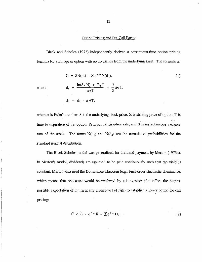
Black and Scholes (1973) independently derived a continuous-time option pricing

formula for a European option with no dividends from the underlying asset. The formula is:

c = SN(dJ) - xe·RrTN(d2), (1)

where dl = ln(S/N) + RrT 1 rNT +- T· rNT 2 '

d2 = d1 - cr.JT,

where e is Euler's number, S is the underlying stock price, X is striking price of option, T is

time to expiration of the option, Rr is annual risk-free rate, and cr is instantaneous variance

rate of the stock. The terms N(d1) and N(d2) are the cumulative probabilities f<i>r the

standard normal distribution.

The Black-Scholes model was generalized for dividend payment by Merton (1973a).

In Merton's model, dividends are assumed to be paid continuously such that the yield is

constant. Merton also used the Dominance Theorem (e.g., First-order stochastic dominance,

which means that one asset would be preferred by all investors if it offers the highest

possible expectation of return at any given level of risk) to establish a lower bound for call

pricing:

(2)

14

That is, the call price must be greater than the stock price minus the present value of

exercise and cumulative dividends (using riskless interest rate).

Stoll (1969) showed that European options exhibit a fixed relationship between the

price of a put and call with the same maturity date, which is denoted as put-call parity

(PCP). Once we know a European call on a stock, we can easily determine the price of the

put on the same stock, regardless of how options are valued. Merton (1973c) showed that

the PCP does not necessarily hold for American options because the possibility of early

exercise cannot be ruled out when the portfolio is established. Klemkosky and Resnick

(1979) tested the put-call parity by using market data from July 1977 through June 1978.

Their results were consistent with the put-call parity.

Risk Premium and the CAPM Model

Risk premium begins with an assumption that all individuals are risk averse. From

the concave utility function of wealth, a convex, positively-sloped indifference function of

expected return and risk is developed, implying a positive substitution between expected

returns and risk. Given an efficient set of portfolios (a set of mean-variance choices from

different combinations of securities), an optimal choice is reached at point A where the

trade-off between the expected return E(R) and risk c?R is in equilibrium (Figure 2).

15

Figure 2. Optimal Portfolio Choice for a Ri'sk Averse Investor

and an Efficient Set.

E(R) Indifference Curve

The CAPM model, used to show the existence and level of risk premiums, was first

introduced simultaneously by Treynor (1961) and Sharpe (1963, 1964). Trenyor's

contribution to the theory of finance was to devise a method for predicting the risk premium

and to demonstrate its importance in the behavior of capital markets as well as in portfolio

selection. Both authors reached the conclusion that the only thing investors should worry

about is how much any asset contributes to the risk of the portfolio as a whole (beta). The

model was further developed by Mossin (1966) and Lintner (1969).

The CAPM model is based on the following assumptions:

A, All investors are risk averse and maximize the expected utility of end-of-period wealth.

B, Investors are price takers and have homogeneous expectations about asset returns.

C, There exists a risk-free interest rate (Rr).

D, Total quantity of the assets is given.

E, Assets are frictionless and information is costless.

16

F, There are no transaction costs, such as taxes and restrictions.

Based on these assumption, an efficient market would reach an equilibrium where

riskier assets would have higher expected returns than less risky assets.

Mathematically, CAPM is

(3)

where E(Ri) is expected rate of return of an individual asset: Rr is risk-free interest rate,

E(Rm) is expected rate of return of market portfolio, and Pi is the covariance of returns

between the market portfolio and the risky asset, or beta. The higher the risk (beta), the

higher the expected return [E(Ri)].

Roll ( 1977) argued that the efficiency of the market portfolio and the capital asset

pricing model are inseparable, joint hypotheses, i.e., it is not possible to test the validity of

one without the other.

There are two kinds of risks: systematic and unsystematic risk. Investors can

eliminate all the unsystematic risks by appropriate diversification among risky assets.

Systematic risk is risk which cannot be avoided by diversification. Beta measures

systematic risk and reflects the covariance with the entire market. A portfolio of the entire

market, having a beta of one, generates a return equal to risk-free rate plus the risk

premium.

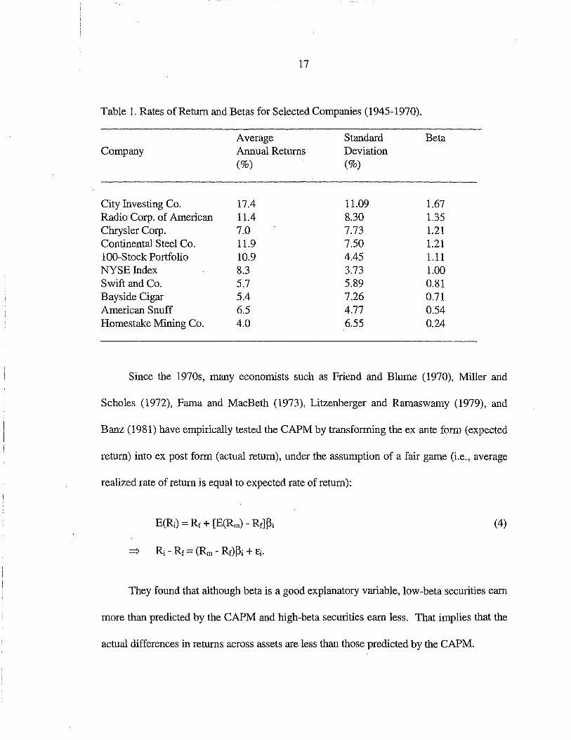
Modigliani and Pogue (1974) found a positive relationship between annual rate of

return and beta (Table 1).

17

Table 1. Rates of Return and Betas for Selected Companies (1945-1970).

Company

City Investing Co. Radio Corp. of American Chrysler Corp. Continental Steel Co. 100-Stock Portfolio NYSEindex Swift and Co. Bayside Cigar American Snuff Homestake Mining Co.

Average Annual Returns (%)

17.4 11.4 7.0 11.9 10.9 8.3 5.7 5.4 6.5 4.0

Standard Deviation (%)

11.09 8.30 7.73 7.50 4.45 3.73 5.89 7.26 4.77 6.55

Beta

1.67 1.35 1.21 1.21 1.11 1.00 0.81 0.71 0.54 0.24

Since the 1970s, many economists such as Friend and Blume (1970), Miller and

Scholes (1972), Fama and MacBeth (1973), Litzenberger and Ramaswamy (1979), and

Banz (1981) have empirically tested the CAPM by transforming the ex ante form (expected

return) into ex post form (actual return), under the assumption of a fair game (i.e., average

realized rate of return is equal to expected rate of return):

(4)

They found that although beta is a good explanatory variable, low-beta securities earn

more than predicted by the CAPM and high-beta securities earn less. That implies that the

actual differences in returns across assets are less than those predicted by the CAPM.

18

Gibbons (1982), Stambaugh (1982), and Shank:en (1985) examined an alternative test

of the CAPM using the following transformation from a two-factor CAPM developed by

Black (1972), in which riskless rate (Rr) is replaced by the return of zero-beta, minimum

variance portfolio (Rz).

E(Ri) = E(Rz) + [E(Rm) - E(Rz)] ~i (5)

~ E(Ri) = Rr(l- ~z) + E(Rm)~i·

Gibbons ( 1982) noticed that there exists a restriction on the intercept of the model:

(6)

Gibbons tested this restriction and found that it is violated, implying the CAPM is rejected.

Arbitrage Pricing Theory (APT), a more general model developed by Ross (1976),

shows that many other factors can explain asset returns. Those factors include such

macroeconomic variables as index of industrial production (or national income), default risk

premium, and unanticipated inflation (Chen etc., 1983). The CAPM can be viewed as a

special case of APT when the market rate of return is assumed to be the single relevant

factor.

Random Walk Theory

As discussed in the introduction of Chapter 4, investors base their decision on the

expected future stock prices [E(S')] rather than the actual future stock prices. Therefore, a

forecast of stock prices is necessary to calculate the expected return from the Portfolio 2.

19

Extensive work has been done to explain and predict the movement of stock prices.

Firm-foundation theory (fundamental analysis) stresses that the value of a stock (or

investment instrument) ought to be based on the,stream of earnings a firm will be able to

distribute in the future (intrinsic value). Castle-in-the-air theory (technical analysis), on the

other hand, focuses on psychic values (beauty contest, i.e., a thing has worth only when

someone else will pay for it) (Malkiel22). However random walk process appears to be the

most commonly accepted model. In this thesis, the random walk model is used to form the

expected stock prices.

The notion of a "random walk" originated in 1959 from "Brownian Motion in the

Stock Market", a paper published by Osborne, which observed that the movement of stock

prices is no more predictable than the movement of an "ensemble" of molecules. Random

walk theory states that the expected return of a security is stationary throughout time, or the

successive price changes are independent and identically distributed.

If St is security price at timet,

(7)

E(Et) = 0,

Cov (Et. Et-I) = 0,

and £- NID (0, O"z).

20

Random Walk Theory asserts that in an efficient market, a security price is random,

not because it is insensitive to any new information, but because it adjusts so quickly to new

information that future stock price changes seem unpredictable.

The weak form of efficiency in Fama's (1970) definition implies that price change

follows a random walk. If unanticipated return is not related to any past information, the

distribution of return conditional on a given past information structure is equal to the

unconditional distribution of return.

Samuelson (1965) showed that prices could follow a deterministic trend while still

fluctuating randomly (random walk with drift). The form is:

(8)

where w is a drift, and E-NID (0, a2).

21

CHAPTER3

THE MODEL

As discussed in Chapter 1, to avoid the problem of adjusting for costs (which vary

from one stock to another) and to correctly value the role of risk aversion in financial

markets, Portfolio 1 and 2 based on one put, one call, and the underlying stocks (S&P 500)

were constructed. The two portfolios have identical costs but have different risks. Risk

premium, defined as market premium per unit of beta in this thesis, should be the difference

between the expected returns from the two portfolios divided by the difference in betas.

Let:

E(S') =

D =

TC =

Rr =

Rp =

N =

Expected S&P 500 price on maturity day.

Future value of accumulated dividend payments (Calculated by using

risk-free interest rate).

Transaction costs and information costs summarized as percentage of

annual rate of return.

Annual real riskless interest rate.

Annual risk premium rate (per unit of beta).

Total number of days before expiration (from the current date to the

maturity date, including weekends and holidays).

22

R1 = Ratio of the maturity-day value to the current -day value of Portfolio 1.

R2 = Ratio of the maturity-day value to the current -day value of Portfolio 2.

The two portfolios involve the following transactions (Table 2):

Table 2. Transaction Summaries For Portfolio 1 and 2.

Asset

Portfolio 1: Portfolio 2:

Current Date

S+P-C S-P+C

Expiration Date

X+D 2S' -X+D

The underlying S&P 500 stock is a representative of the well-diversified market portfolio.

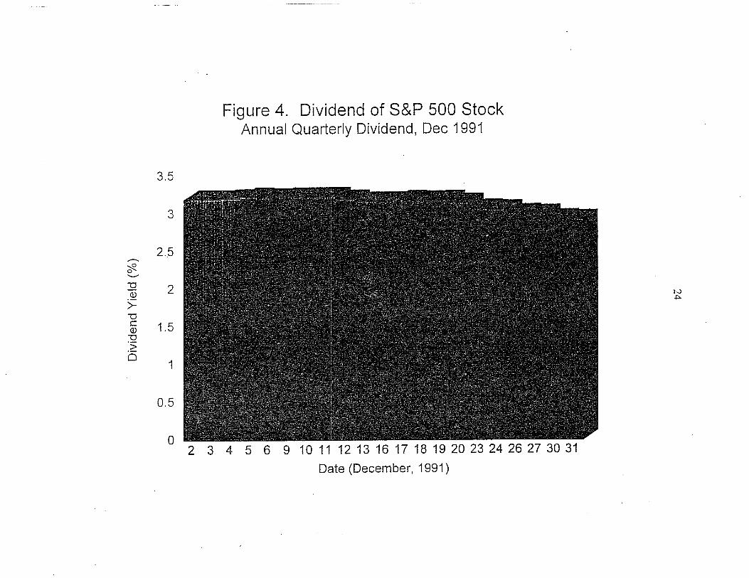
D is assumed to be certain and constant. As shown in Figure 3 and 4, the volatility of

accumulated dividends is very small compared-to that of the stock price. Figlewski (1984)

argued that dividend uncertainty for S&P 500 is insignificant. This assumption implies that

the change of rate of returns is solely from the change in stock price (market appreciation).

Portfolios 1 and 2 have different risks. Portfolio 1 has a beta of 0 and Portfolio 2 has

a beta close to 2 (see Appendix A, Note 1).

According to the CAPM model (Chapter 2, equation (3)),

E(Ri) = Rr+ [E(Rm)- Rd~i (3)

Figure 3. Decompositions of Returns Dividends & Appreciation Jan-Jun 1992

0.3 '

0.2 -~---~------------c 1-:::J

a> 0::: 0.1 0 Q)

-ro 0::: 0 rn E 0 z - -0.1 rn :::J c c <(

-0.2

-0.3 l.T~wr•·•·T*I'"'r"·'- "~'"f""'"r' l'''"j"'u''"W'1""'m""r,TT'·Ir"1'TTT'rwf"JT"'"T'J Times Series Data Jan-Jun 1992

lll TOTAL DIVIDENDS J Ill MARKET APPRECIATION -·-· -------··-··--------

N l.J,)

3.5

3

2.5 .--. ~ 0 ........-u 2 Q)

>-u c 1.5 Q) u :~ 0

1

0.5

0 2 3

Figure 4. Dividend of S&P 500 Stock Annual Quarterly Dividend, Dec 1991

4 5 6 9 10 11 12 13 16 17 18 19 20 23 24 26 27 30 31 Date (December, 1991)

t.J .j:>..

25

That is, the expected rate of return of a risky asset is the linear combination of risk-free rate

and risk premium times its beta (systematic risk).

In this study, since

and so:

X+D and R2 =

S+P-C

2E(S) -X + D

S- P +C

R = 1 + (Rr + TC)*N /365 + ~*Rp*N/365 +E. (9)

where 365 is the number of days in 1992 and when R = R1, ~ = 0, and when R = R2, ~ = 2.

Based on the previous analysis, Rr (real risk-free rate or opportunity costs) and TC

(transaction costs and information costs) are constant in both portfolios. The real Treasury

Bill rate is used as real riskless rate in this thesis.

The error term (E) reflects market noise and degree of market inefficiency. Black

points out that noise is the primary motivation of market activity. Market noises also reflect

the degree of understanding of the real world as well as degree of market efficiency. In this

thesis, the error terms in both portfolios are assumed to have the same variance (i.e., the

same degree of market efficiency).

The statistical form is as follows:

Ri = a+ b*N/365 + c*Di*N/365 + Ei, (9*)

where D is a dummy variable of beta, D = 0 when R1 is used, D = 2 when R2 is used, and

Ei ~Nro co. cr)

26

It is expected that

1. a= 1,

2. b = Rr + TC > Rr, and

3. c is a test of the existence and level of the risk premium.

To remove the effect of inflation from the returns, Rl and R2 were deflated by the

actual inflation rate. V arlo us inflation rates have been suggested. Since the primary

concern is the difference between Rl and R2 as measured by c, the analysis is unlikely to be

sensitive to minor differences among alternative choices of the inflation rates.

27

CHAPTER4

EXPECTED STOCK PRICE

All of the variables used to calculate R1 and R2 are directly observable except E(S'),

the expected future stock prices. Many economists avoid this problem by simply 'using the

actual stock prices at the expiration date (S') as an unbiased instrument of E(S'), justified by

the efficient-market theory.

The data set in this thesis (from January 2, 1992 through June 30, 1992) is relatively

short and the short-term variations may adversely affect the results. The S&P 500 during

that period is generally a bear market (Figure 5). Replacing E(S') by S' would therefore

result in a negative risk premium. Nor can we use S for E(S') because under zero drift R2 is

always smaller than R1 (see the mathematical proof in Appendix A, Note 2).

Various approaches to the formation of expected stock prices E(S') based on the

random walk theory were investigated.

Testing Random Walk

The most commonly accepted stock market movement pattern is the random walk. In

a random walk, price changes do not follow a pattern and past information is useless in

Figure 5. S&P 500 Market Prices Januat)i- June 1992, In Norminal Terms

425~----------------------------------------~

-. ~420 en Q) 0

~ 415 ~ 0 .8 CJ) 410 Q) Cl ~ Q)

~ 405 ~ "(ij 0 400 0 0 1.0 0.. c6 395 CJ)

390 Jliilliiiiilillilllllliillillillilliillllilliilllilllilililililiiilliiilliilllililil!llillililliiillliilllilliilliilliiillillli'

10 00

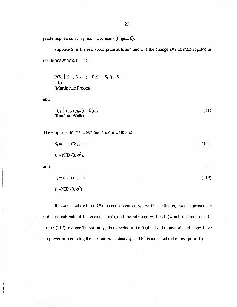
29

predicting the current price movements (Figure 6).

Suppose S1 is the teal stock price at time t and r1 is the change rate of market price in

real terms at time t. Then

and

E(St I St-t. St_z, ... ) = E(St I St-1) = St-1 (10) (Martingale Process)

E(rt I rt-t. rt-2, ... ) = E(rt), (Random Walk).

The empirical forms to test the random walk are:

St=a+b*St-1 +Et

Et ~ NID (0, cr),

and

rt = a+ b rt-1 + Et

Et ~ NID (0, cr)

(11)

(10*)

(11 *)

It is expected that in (10*) the coefficient on S1•1 will be 1 (that is, the past price is an

unbiased estimate of the current price), and the intercept will be 0 (which means no drift).

In the (11 *), the coefficient on r1_1 is expected to be 0 (that is, the past price changes have

no power in predicting the current price change), and R2 is expected to be low (poor fit).

---------~ -------------- ------------------ ·- -·-- --·-· ----· -----·······-- -- .. .... ·- .... ----- ..

Figure 6. Random Walk - S&P 500 Returns in Real Terms, 1941-1991.

40.------------------------------------------------

.......... eft 30 ............ c 0

+:: ctl

'(3 20

~ 0. 0. <( 10 ...... Q) ~ '-ctl

-l------111

~ 0 Jl, J '-1-' I ' . ' ______J_ • J L I \}--- 111 I I 11 I 1 I I I I ctl :::s c c <( -10 0 0 l()

a. o6 -20 (/)

-30 ~1 143 145 '4'7 149 's1's3 's5 's'7 's9 '61 163 165 16'7 169 171'73i75'7'7 179 's1's§ 'sf'87'89-·'91

Year

-----·-------·----·-·----

w 0

31

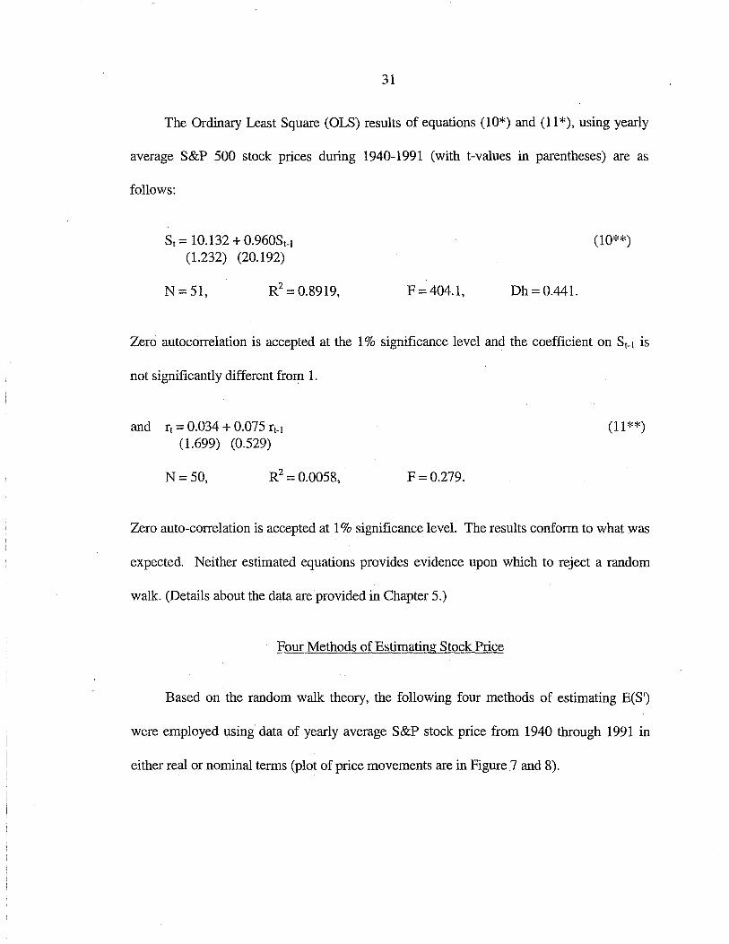
The Ordinary Least Square (OLS) results of equations (10*) and (11 *), using yearly

average S&P 500 stock prices during 1940-1991 (with t-values in parentheses) are as

follows:

St = 10.132 + 0.960St-1 (1.232) (20.192)

N=51,

(10**)

F=404.1, Dh=0.441.

Zero autocorrelation is accepted at the 1% significance level and the coefficient on St_1 is

not significantly different from 1.

and rt = 0.034 + 0.075 rt-1 (1.699) (0.529)

N=50, R2 =0.0058,

(11 **)

F = 0.279.

Zero auto-correlation is accepted at 1% significance level. The results conform to what was

expected. Neither estimated equations provides evidence upon which to reject a random

walk. (Details about the data are provided in Chapter 5.)

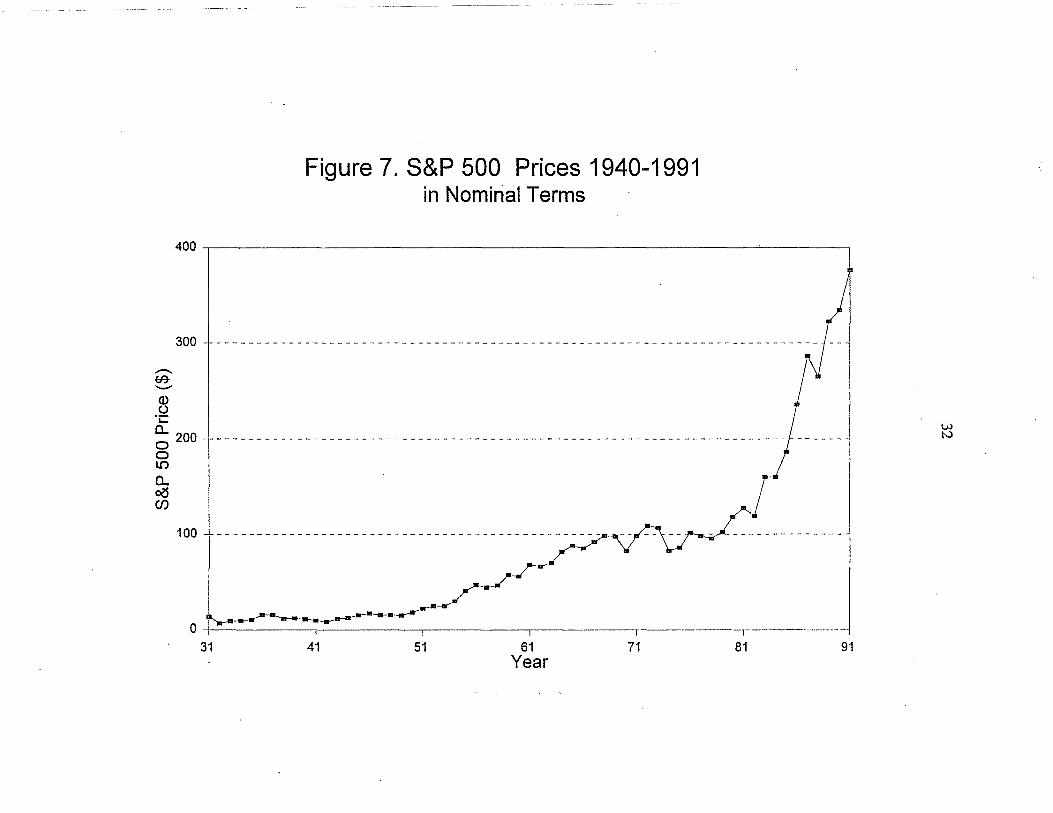
Four Methods of Estimating Stock Price

Based on the random walk theory, the following four methods of estimating E(S')

were employed using data of yearly average S&P stock price from 1940 through 1991 in

either real or nominal terms (plot of price movements are in Figure 7 and 8).

-Ef7 ...._ Q)

.2 '-

Figure 7. S&P 500 Prices 1940-1991 in Nominal Terms

400 ---,

300 ----------------------------------------------------------------------------~--~

0.. 0 200 0 1.0

~ I 100 -l---- ---------------------------------;~7v:v/L _______ _

0 ----- ,.-../ -·---------·-·___..------r"" 81 -31 41 51 61

Year 71 91

w N

-·-- ---····---------- ---------···--·····------- - ------·- ··-·----·--

Figure 8. S&P 500 Prices 1940-1991 Inflation Adjusted (1982=1 00)

3.----------------------------------------------------------------------------------,

en Q) u ·c

2.5

c. 2 ~ u 0 .....

(J)

0 0 1.0 1.5

CL ~ (J)

l

----- --- -------- -- ----- ---~- -- --- -- -- ---------- -----_,... ... ---- -- ---~- -r··-· --- -------_ _,..\j

y'\_/ 0.5 r·,.-.,--.,.-.,.-,.--r

w w

34

Method 1

Based on the earlier discussion in this Chapter, the movement of stock price in real

terms is assumed to be a random walk, and the expected stock price in nominal terms is

therefore the past stock price plus the expected inflation rate. In this model, it is assumed

that the expected inflation rate is formed in such a way that people adjust their expectation

according to the past inflation.

Suppose:

that:

and

S't =

E(S't) =

E(1tt) =

Nominal stock price at timet,

Inflation rate at given time t,

Expected nominal stock price at time t,

Expected inflation at time t,

E(S't) = S't-1*(1 + E(1tt))

E(1tt) = a + b1tt-1

Taking the natural logarithm of both sides:

=:} Ln E(S't) = Ln S't-1 + Ln(l + E(1tt))

Ln S't = Ln S't-1 + b*Ln(l + E(1tt)) + Et

E-NID (0, cr)

and =:} 1tt =a+ b*1tt-1 + !lt

J..L- NID co, cr)

(12)

(13)

(12*)

(13*)

35

Equations (12*) and (13*) were estimated by a two-stage process. The predicted

value (1tt*) was used for E(7t) in estimating (12*), with a restriction of 1 on the coefficient of

Ln S\.1. The OLS regression results are:

1tt* = 0.023 + 0.5051tt-1 (3.033) (4.061)

N=50,

and Ln S't= Ln S\.1 + 1.06 Ln ( 1 + 1tt*) (2.812)

N=50, R2 = 0.9813,

(13**)

F= 16.5, Dh= 1.56.

(12**)

F = 52152, DW= 1.521.

Second-order serial correlation is not significant at the 1% level in either of the regressions.

The actual and predicted inflation rates, (1tt and 1tt\ are shown in Figure 9. The predicted

inflation rate for 1992 is 0.0429. The estimated equation (12**) will be used in calculating

the expected value of S&P 500 on the expiration date.

E(S'i) = exp(Ln Si + 1.061 Ln(l + 0.0429*N/365)),

· whereE(S'i) is in nominal terms.

Method 2

Since E(St I St-I. St-z, ... ) = E(St I St-1), the expected real price St is formed upon St-1

only. Then:

St = a+ b*St-1 + Et (14)

Et - NID (0, cr),

...-..

FIGURE 9. ACTUAL VS EXPECTED INFLATION 1942-1991

0.25 -.---------------------:-------

0.2 ------6h----------------------------------------------------------------

~ 0.15 UJ

~ z 0.1 0

~ u.. z

0.05

0+----~-----------------------

-0.05 421 I 46 1 I 156

I I 154

1 I 158

1 I 62 1 1'66' I 176

I IT74

I I 178

1 I 182"18GTI""Igor

52 64 68 72 76 80 84 88 YEAR

---···· -~-------- ----·----·-11 1-•- ACTUAL INFLATION _-+·-· EXPECTED ~~~~T~~~__I

w 0\

37

where a is expected to equal 0 and b is expected to equal 1. The OLS results (with t-values

in parentheses) are:

Sr = 10.132 + 0.960Sr-I (1.232) (20.1)

N=51, ?

R- = 0.8919,

(14*)

F=404.1, Dh=0.441.

Second-order autocorrelation is not significant. Although a minimum drift can't be

significantly rejected from this regression, the empirical form (14*) was used to compute

the expected stock price.

Method 3 and 4, Estimating a Specific Drift in Real Terms

If the investor expects stock prices to drift, then the drift will affect the stock price

and thereby the expected rate of return in Portfolio 2 as:

R2 = 2E(S) - X + D S(l + w * N I 365) - X + D =

S - P + C S - P+C (15)

where w is the real, annual drift, and S is S&P 500 stock price at current time.

Following are two methods of estimating the drift, w.

Method 3 (Arithmetic Market Price Appreciation Rate). From the historical data of

the S&P 500 (1940-1991), the average annual nominal market appreciation is 7.98% and

38

Method 4 (Geometric Market Price Appreciation Rate). Suppose a long-run price

trend is an unbiased estimate of the expected drift. From historical data, during the 50-year­

period from 1941 through 1991, the S&P 500 stock price appreciated in nominal terms at a

compounding annual rate of 7.6%, while the overall price index (using the GNP implicit

deflator) increased at a compounding annual rate of 4.7%. The real capital gain, which is net

of inflation, is therefore 2.9%.

39

CHAPTERS

DATA

The two sets of data in this thesis are discussed below.

The First Data Set

The first set is the data used in testing for the random walk and estimating the

expected appreciation in S&P 500 stock price. The S&P 500 yearly average stock prices

\ from 1940 through 1991 were collected from the 1994 Price Index Security Record

published by Standard and Poor's Statistical Reporting Service. The annual price index,

which is used to deflate nominal stock price into real terms, was obtained from the Gross

National Product (GNP) implicit deflator in the Economic Report of the President, 1992.

The price index for 1992 was constructed from a Gross Domestic Product (GDP) index

because the GNP index was not found

The Second Data Set

The second data set is used to estimate the risk premium by comparing the two

portfolios constructed from S&P put and call options. The S&P 500 option was used

40

because it is a European type option, and thus the .put-call parity (PCP) strictly holds

(Merton 1973b).

The data are from January 2, 1992 through June 30, 1992. There are 148,192

observations and 44,704 observations respectively, in the original cash price and option

price data. The data were purchased from Future Industry Institute, located in Washington,

DC. Because the large data set was cumbersome, it was compressed by using the daily

average value as an observation for each variable. This reduced the number of observations

to 935.

The Treasury Bill (T-Bill) rate was used as the risk-free interest rate. Daily T-Bill

rates were collected from the Wall Street Journal. For each option type, the Treasury Bill

rate whose maturity date was closest to the option's expiration date was used.

The dividend payments for each business day were also collected from the Wall

Street Journal. From the daily data, the future value (at maturity day) of the accumulative

dividends was calculated using the T -Bill rate as the discount rate.

The data set analyzed contained 935 observations on the following variables: current

date, type of contract, expiration date, exercise price (X), future accumulated dividends (D),

call price (C), put price (P), current stock price (S), actual stock price at maturity (S'),

number of days before expiration (N), and T-Bill rate (TBILL). Those data were sorted first

by date, then by the type of contract (first by maturity day, then by strike price). The first

935 observations are Portfolio 2 and the second 935 observations are Portfolio 1.

41

A sample of the data (first 50 observations) is included in appendix B . The actual

inflation rate in 1992 used to deflate returns was 2.78%, which was calculated from the

GDP implicit price index (U.S. Congress, p272).

42

CHAPTER 6

EMPIRICAL FINDINGS

OLS Estimation

E(S ') were calculated by the four methods discussed in chapter 5. Table 3

summarizes the four estimation methods. Rl and R2 in real terms were obtained using the

following formula (16). 1r is inflation adjustment factor.

Table 3. Summary of Four Estimation Methods Used to Estimate E(S ').

Method No. Brief Description Estimated E(S')

1 Expected nominal stock price is based upon equation past stock price plus expected inflation (12**)

2 Real stock price is formed only on past equation real stock price (14*)

3 Real, long-run arithmetic drift market price appreciation (w = 3.28%)

4 Real, long-run geometric drift market price appreciation (w = 2.9%)

43

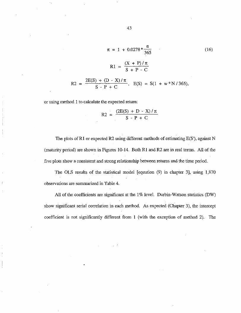
n 7t = 1 + 0.0278 * 365

R1

= (X + P) I 1t

S+P-C

R2 = 2E(S) + (D - X) I 7t , E(S) = S(l + w * N I 365), s- p + c

or using method 1 to calculate the expected return:

R2

= (2E(S) + D - X) In s- p + c

(16)

The plots ofR1 or expected R2 using different methods of estimating E(S'), against N

(maturity period) are shown in Figures 10-14. Both R1 and R2 are in real terms. All of the

five plots show a consistent and strong relationship between returns and the time period.

The OLS results of the statistical model [equation (9) in chapter 3], using 1,870

observations are summarized in Table 4.

All of the coefficients are significant at the 1% level. Durbin-Watson statistics (DW)

show significant serial correlation in each method. As expected (Chapter 3), the intercept

coefficient is not significantly different from 1 (with the exception of method 2). The

Figure 10. Plot of R1 Against N In Real Terms, 935 ObseiVations

t.01-r-----------------------.

1

E 1. .a Q) a: 1. 0 E 1. m a: J9

-------------------------------------------------:!!·--.------·::::::::::::::::::::::::::::::::::::_ '!lo...... + + ~ ------------+ ... + + -------=----- .. ...._ + -----+ .. __ ... _____ ..,____ * + •:~~o .... ""' """-------------·-----------+--.... ..m... + ... ~ ;~· ~~_!_·-------~----...... + -. ...... :!IJIIIII ~- ----..i,."'ft- ++ +

• + ----+- .. ----:S: '~~~- 6 -~~-A-~-----,++ - ~ :t*: ~-~ "!:---+------------~- . ._f.! ··~~r :L~·-~"!~ Jillll:" .... ...... ---- + .... -- ---- .......

...,.. ..... ~ .. - ... ll'- + * ... * -------·- . + + ----------+ ... ... + ------------.... + .. . --------=..: --------- ----... ...

~ O.OOA~-..; -------- ... . ------------------------------------... -*----------· ~--------------- + -------"lfl ...

~ I+ ----------------------------------------------------------------------------------a: 0 .996i-:.: ----t··-¥---------- + ------------------------------

----------~----·--·············+·-~----·····------------------------------0

0009 + 0 20 40 60 80 100 120

N: Number of Days Before Expiration

t

Figure 11. Plot of R2 Against N Method 1 , In Real Terms, 935 Obs

1.01~---------------------.

E ::J ......... Q)

a: 0 Q) 1. n1 a:

·····························;;········----~---.. -·-··········:::::::::::::::::::::::::::::· ·:·········:.:·· ... ·······-"'·-·······:.-··--+ ;···· + + ....

... .... .. +---··.;.:··· :1: + -.;..._... .,. --~----······· +-·· ~ + ..... + ..... .... + ·;,;···... ........... .. ,iii. + ..... ~: .. ;li; ....... ··;,::;·.;,. + + +

. ...... ...... - ... ,.. .• - ~ ... *"' +11: !I! ..... :1: 11<-- ... , ... ~ ........... ~ + ..... •'! ....•........... b ~ -~~.!fLiiio.+ .• ---- + t.

................ + ! + + :t + : ..................... . + + ... ... -----------....... ... -·------11111 .. ------------ + -~--- ... ...

LALA~-+-·····.U.···~·-························································································· ... ... ... ----------~---·-----~----------+·-~---------------------------------------------------------------------

... 0 20 40 60 80 100 120

N: Number Of Days Before Expiration

.j:>. Vl

---~ ----- --------

Figure 12. Plot of R2 Against N Method 2, In Real Terms, 935 Obs

O.~f3E>-t---------- ---------------------··;;··--------------------------- .. ~ .. +

~------~ ~-----------------

---------- .. .. + ... , --------------

.. .. ·=------------~--------.. ----:t.11" _*!!. j;O.i; *"' ...... : ---0 Q)

05 0. a:

~ ~

0. (}~k ...... -ollll ....

0

+ • I" r ,.~ -----·----- ,. ~ ~ ------ .. ~-t...! . ..C :b" ~ .. ----------------------

~- ......... ---~- -.. ,., ......... .--.;r-•• + .,--9- -----~--.:.... 11: ---- -------------------------- ----

+

+ +

+

2() 4() 6() 8() 100 120 N: Number of Days Before Expiration

~ 0\

Figure 13. Plot of R2 Against N Method 3, (3.28°/o Drift), In Real Terms

1.04·~-----:---__:_------------....

.

E: ----·::::::::::::::::::::::::::·--------------------------------------------------------:J ----------- .. ----------~ Q5 1.025 ------------- --------------------------- .. t + + -·····-··

a: -------------- .. ..,.._~~ ..;:;. --- --------------------- .. ~lll" --.,.------------0 -------------------- .. -------- _* _____ ,~_:.':__ --- -· * 1 01 ---------·-+----c-!.., ..... ~ ... -----------------------------0: - 5 --------------------- • ~ - _.,..,,.___ __ _ ----~-~11111: ~ -.:" ---------------------

. - ~~: ______ :_:::::::::::·---------------------------------::::::::·

~ 1.01

"-i 1. a:

0

+ + ......... .

·····---~---·····-········-··-···-··········-::::::::::::::::::::::::::::::::·

20 40 60 80 100 120 N: Number of Days Before Expiration

~ -...)

c 1-

::J 1i5 - 1. a: -~ 1.()1 10 a: 1.()1 co 0 1- 1. ~

Figure 14. Plot of R2 Against N METHOD 4 (2.9o/o Drift), In Real Terms

::::::::::::::·:::::·:::::·:········································-,..·········· .. ..... :: ----------- + ++ f ... •---------························ .. ..a .. . ....

......... "' ----- -.... ............ + =!: & .--~- ..... ------------- ------------~--.. ----in-~:~;~--- -------------------------------------------------ooo.--~~-~~---- ............................... .

... ~* -·····-·········

~---·······································::::::::::::::::::::: +

+ -+···········--··················································--·--·

+ () lJlJ~-T-~---··-··---------------------------------------·--·········-··-------------------------------------------

() 2() 4() 6() 8() 1()() 12() N: Number of Days Before Expiration

+:-. 00

49

coefficient on N/365, Rr + TC, is around 1.6%. The estimated risk premium is significant

with a range from 3% to 5% (method 2 produces a negative premium).

Method 2 produces a negative premium and an intercept less than 1 because the

model [equation (14)] used to predict the expected price is simple and open to over- or

under-forecasting from year to year. It generally undervalues the expected price in 1992.

The rate of return and risk premium (Rp) using method 2 is therefore underestimated.

Table 4. OLS Estimation of Coefficients in Equation (9), Using 935 Observations.

Method Intercept Rt+ TC F RHO DW

1 0.99997 0.0159 0.034 0.8474 5198.7 0.424 1.15 (0.00008) (0.0009) (0,0005)

2 0.98465 0.127 -0.094 0.5184 1004.7 0.694 0.611 (0.00004) (0.0041) (0.0021)

3 0.99997 0.0159 0.049 0.9140 9918.4 0.611 0.775 (0.00008) (0.0009) (0.0005)

4 0.99997 0.0159 0.046 0.9020 8591.8 0.611 0.774 (0.00008) (0.0009) (0.0005)

(DW is Durbin-Watson Statistics. RHO is estimated first-order auto-correlation coefficient in error terms. Standard deviations are in parenthesis.)

Table 5. Statistics Summary of The Treasury Bill Rate, January- June, 1992.

Mean Standard Deviation Maximum Minimum

3.68% 0.22% 3.07% 4.17%

50

The T-Bill rate was not employed as an explanatory variable in this thesis because the

testing period is short (from January to June, 1992) and the Treasury Bill rate is relatively

stable in this period (see Table 5).

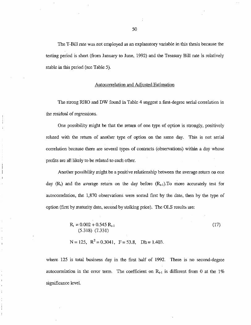
Autocorrelation and Adjusted Estimation

The strong RHO and DW found in Table 4 suggest a first-degree serial correlation in

the residual of regressions.

One possibility might be that the return of one type of option is strongly, positively

related with the return of another type of option on the same day. This is not serial

correlation because there are several types of contracts (observations) within a day whose

profits are all likely to be related to each other.

Another possibility might be a positive relationship between the average return on one

day (R1) and the average return on the day before (R1-J).To more accurately test for

autocorrelation, the 1,870 observations were sorted first by the date, then by the type of

option (first by maturity date, second by striking price). The OLS results are:

Rt = 0.002 + 0.545 Rt-1 (5.318) (7.331)

N = 125, R2 = 0.3041, F = 53.8, Dh = 1.403.

(17)

where 125 is total business day in the first half of 1992. There is no second-degree

autocorrelation in the error term. The coefficient on Rt-1 is different from 0 at the 1%

significance level.

51

Since autocorrelation exists in the returns of consecutive days, OLS estimation is,

though unbiased, not efficient. To correct for the serial correlation, a uniform time-series

cross-sectional pooled data set was constructed in which each cross-section contained a time

series of 23 observations. Each observation within a cross-section has the same strike price

and maturity date. From the original 935 observations, 19 cross-sections, each containing

23 observations (a total of 437 observations) were used as a new data set to examine the

influence of the serial correlated errors. The total number of observations available for the

regression is 874. Details ofthe data processing are provided in Appendix A, Note 3.

Table 6 summarizes OLS results of the statistical model [equation (9)], using the

second set of data (87 4 observations). The results are very close to those estimated for the

entire sample in Table 4, indicating little effect from truncating the data set. The RHO in

Table 6 is generally lower than that in Table 4 because the RHO in Table 6 only accounts

for correlation between the days.

Assuming a constant autocorrelation coefficient across types of contract (cross-

section), the statistical form of the model (Krnenta, 1986, 616) is:

where

Rit = a + b*Ntf365 + C*D*Nit/365 + Eit.

Rit = Rl, if D = 0

Rit = R2, if D = 2

E( ) t-s 2 Eit. tis = P (j'i , (t > s).

(i -:F j).

(18)

52

Table 6. OLS Estimation of Coefficients in Equation (9), Using Cross-sectional Time-Series Data (874 Observations).

Method Intercept Rt+TC Rp R2 F RHO DW

1 1.0000 0.0162 0.035 0.8682 2869.3 0.469 1.058 (0.0001) (0.0013) (0.0006)

2 0.98471 0.130 -0.096 0.6418 780.3 0.900 0.203 (0.0006) (0.005) (0.0025)

3 1.0000 0.0163 0.050 0.9269 5523.6 0.467 1.063 (0.0001) (0.0013) (0.0006)

4 1.0000 0.0163 0.046 0.9164 4775.9 0.467 1.063 (0.0001) (0.0013) (0.0006)

(Standard deviations are in parentheses.)

The statistical results after adjusting for cross-sectional heteroskedasticity and time-

series autoregression are presented in Table 7. The estimated RHO for each method is

significant and similar to those reported in Tables 4 and 5. Rr + TC is estimated to be

approximately 1.5%. Sinc1:1 the real riskless treasury rate during the first half of 1992

averages 0.9% (the average nominal T-Bill rate in 1992 is 3.68% as shown in Table 5 and

the expected inflation rate in 1992 is 2.78%), the estimated transaction costs plus

information costs equal 0.6% (1.5% - 0.9%). Since the T-Bill rate of 3.68% does not

include any implied costs such as commissions, and so the real opportunity cost must be

smaller than 3.68%, the estimated transaction costs plus information costs actually exceed

0.6%. This number coincides with the fee charged by most financial companies. For

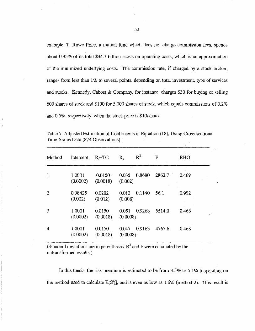
53

example, T. Rowe Price, a mutual fund which does not charge commission fees, spends

about 0.35% of its total $34.7 billion assets on operating costs, which is an approximation

of the minimized underlying costs. The commission rate, if charged by a stock broker,

ranges from less than 1% to several points, depending on total investment, type of services

and stocks. Kennedy, Cabots & Company, for instance, charges $30 for buying or selling

600 shares of stock and $100 for 5,000 shares of stock, which equals commissions of 0.2%

and 0.5%, respectively, when the stock price is $10/share.

Table 7. Adjusted Estimation of Coefficients in Equation (18), Using Cross-sectional Time-Series Data (874 Observations).

Method Intercept Rt+TC Rp Rz F RHO

1 1.0001 0.0150. 0.035 0.8680 2863.7 0.469 (0.0002) (0.0018) (0.002)

2 0.98425 0.0202 0.012 0.1140 56.1 0.992 (0.002) (0.012) (0.008)

3 1.0001 0.0150 0.051 0.9268 5514.0 0.468 (0.0002) (0.0018) (0.0008)

4 1.0001 0.0150 0.047 0.9163 4767.6 0.468 (0.0002) (0.0018) (0.0008)

(Standard deviations are in parentheses. R2 and F were calculated by the untransformed results.)

In this thesis, the risk premium is estimated to be from 3.5% to 5.1% [depending on

the method used to calculate E(S')], and is even as low as 1.6% (method 2). This result is

54

305) estimated that the risk premium during the 1980s was about 4 to 6 percentage points.

Van Home (1992, p. 74) concluded that the expected market risk premium has ranged from

3 to 7 % in recent years.

Heteroskedasiticity

Heteroskedasticity was previously suspected in this model because the variance of

returns from the two portfolios could possibly increase with N, the time period before

maturity. However, as shown in Figures 10-14, the variance of returns seems to have no

significant relationship with the number of days to maturity. Using White's test, in which N

is treated. as an explanatory variable, heteroskedasticity was found to be insignificant

(details of testing is in Appendix A, Note 4).

Summary of Empirical Results

The empirical results of this study are summarized below.

(1) The high R2 and F value indicate that the proposed model, based on the put-call

parity, fits well overall. The estimated opportunity costs plus transaction costs and

information costs (Rr + TC), is significant and at least 1.5% (autocorrelation-adjusted

estimation). Transaction costs and information costs are estimated to be at least 0.6% in the

financial markets.

(2) The estimated risk premium varies from 3.5% to 5.1 %, except in method 2 which

estimates the risk premium at 1.6%. These results are similar to the risk premium estimated

in most of the literature.

55

(3) The estimated correlation of today's average returns with yesterday's average returns

is 0.5 (Equation 17 and Table 7). About half of the autocorrelation can be explained by the

data averaging process (see Working 1960), leaving the other half unexplainable. If the

market is efficient and provides no arbitrage opportunities, especially over a longer period,

this finding implies a possible misspecification in this model. However, if the possible

misspecification affects both portfolios similarly, the estimated risk premium may still be

reliable.

(4) White's test does not show strong heteroskedasticity when N, the time until maturity,

is used to explain the variance.

(5) Historical yearly average S&P 500 price (1940-1991) shows that random walk holds

in real terms (refer to Chapter 4).

56

CHAPTER 7

CONCLUSIONS AND REMARKS

The CAPM model begins with the premise that all investors are risk averse and that

risk is not escapable. · Previous estimates of risk premium have not been separated from the

transaction costs, information costs, and default costs. After adjusting for the transaction

and information costs, risk premium (Rp) ranges from 3.6% to 5.1 %.

The empirical estimation of Rp is based on how stock price expectation was formed.

However, the choice of method used does not strongly affect the conclusion reached. Table

8 summarizes the results of risk premium per unit of beta estimated by Proposed model and

by the CAPM model, under method 1,3 and 4.

Table 8. Comparison of Rp by Proposed Model and Rp Estimated by the CAPM Model.

Method No.

1

3

4

This model Rp (%)

3.4

4.9

4.6

Std. Dev. (%)

0.05

0.08

0.08

CAPM Rp Difference (%) (%)

4.00 -0.60

5.52 -0.62

5.14 -0.54

(Those estimates are the means of the total 935 observations adjusted to an annual rate, without considering any autocorrelation.)

57

The difference between the risk premium estimated by this model and that estimated

by the CAPM model is significant and stable, though small, regardless of which method is

used to estimate the expected return (see mathematics discussion in appendix A, Note 5).

Theoretically speaking, the difference in risk premium between the two models should be

equal to the summation of transaction and information costs. The transaction and

information costs estimated in this study are about 0.6% (Chapter 6), which is very close to

the differences shown in Table 8.

The costs associated with Portfolios 1 and 2 are not strictly identical because Portfolio

1 does not contain any default risks and· default costs. The estimated risk premium is

therefore larger than the theoretical or pure risk premium because it picks up the default

costs existing in R2 only. Since dividends account for a large portion of total returns (about

2/3 in put-call parity) and are not strictly constant, the beta of Portfolio 2 is not strictly equal

to 2 (Refer to Appendix A, Note 1). Its variance, as well as correlation with the market

appreciation, needs further research.

Another limitation of this thesis is availability of the data. Although long-term data

do not necessarily eliminate the need for a stock price expectation model, the actual returns

also could be compared because both realized returns and risk premium are fairly easy to

calculate.

58

REFERENCES CITED

59

REFERENCES CITED

Banz, Rtof W. "The Relationship Between Return and Market Value of Common Stocks." Journal of Financial Economics 9(1), March 1981: 3-18.

Benjamin, Daniel K. "The Use of Collateral to Enforce Debt Contracts." Economic Inquiry 16(3), July 1978: 333-359.

Black, Fischer. "Capital Market Equilibrium with Restricted Borrowing." ·Journal of Business 45(3), July 1972: 444-455.

Black, Fischer., and Myron S Scholes. "The Pricing of Options and Corporate Liabilities." Journal of Political Economy 81(3), May-June 1973: 637-654.

Chen, N. F., R. Roll, and S. Ross. "Economic Forces and the Stock Market: Testing the APT and Alternative Asset Pricing Theories." Unpub. Working Paper No. 20-83, Graduate School of Management, University. of California at Los Angeles, December 1983.

Coase, R. H. "The Nature of the Firm." Economica, New Series, IV (1937): 386-405. Reprinted in Reading in Price Theory. Homewood, IL: Irwin. 331-351.

Fama, Euqene F. "Efficient Capital Market: A Review of Theory and Empirical Work." Journal of Finance 25(2), May 1970: 383-417.

Foundation of Finance. New York: Basic Books, 1976.

Fama, Euqene F., and James MacBeth. "Risk, Return, and Equilibrium: Empirical Test." Journal of Political Economy 81(3), May-June 1973: 607-636.

Figlewski, Stephen. "Hedging Performance and Basic Risk in Stock Index Futures." Journal of Finance 39(3) ,1984: 657-669.

Friend, Irwin, and Marshall Blume. "Measurement of Portfolio Performance under Uncertainty." American Economic Review 60(4), September 1970: 561-575.

60

Gibbons, Michael R. "Multivariate Tests of Financial Models: A New Approach." Journal of Financial Economics 10(1), March 1982: 3-28.

Gould, John P., and D. Galai. "Transactions Costs and the Relationship Between Put and Call Prices." Journal of Financial Economics 1(2), July 1974: 105-129.

Grossman, Sanford J., and Joseph E Stiglitz. "The Impossibility of Informationally Efficient Markets." American Economic Review 70(3), June 1980: 393-408.

Klemkosky, Robert C, and Bruce G Resnick. "Put-Call Parity and Market Efficiency." Journal of Finance 34(5), December 1979: 1141-1155.

Kmenta, Jan. Elements of Econometrics. 2nd ed. New York: Macmillan Publishing Co., 1986.

Latham, M. "Defining Capital Market Efficiency. Unpub. Finance Working Paper No. 150, Institute for Business and Economic Research, University of California at Berkeley, April1985.

Lintner, John "The Aggregation of Investor's Diverse Judgements and Preferences in Purely Competitive Security Markets." Journal of Financial and Quantitative Analysis 4(4), December 1969: 347-400.

Litzenberger, Robert H, and Krishna Ramaswamy. "The Effect of Personal Taxes and Dividends and Capital Asset Prices: Theory and Empirical Evidence." Journal of Financial Economics 7(2), June 1979: i63-195.

Malkiel, Burton G. A Random Walk Down Wall Street. New York: W. W. Norton & Company, 1985.

Merton, Robert C. "An Intertemporal Capital Assets Pricing Model." Econometrica 41(5), September 1973a: 867-887.

"The Relationship Between Put and Call Option Prices: Comments." Journal of Finance 28(1), 1973b: 183-184.

"The Theory of Rational Option Pricing." Bell Journal of Economics and Management Science 4(1), Spring 1973c: 141-183.

Miller, M., and M. Scholes. "Rates of Return to Risk: A Re-examination of Some Recent Findings." Studies in the Theory of Capital Markets. Ed. Michael C. Jensen. New York: Praeger, 1972. 47-78.

61

Modigliani, F., and G. Pogue. "An Introduction to Risk and Return." Financial Analysts Journal30 (March-April 1974): 68-80, and 30 (May-June 1974): 69-85.

Mossin, J. "Equilibrium in a Capital Asset Market." Econometrica 34 (October 1966): 768-783.

Phillips, Susan :M., and Clifford W. Smith. "Trading Costs for Listed Options: Implications for Market Efficiency." Journal of Financial Economics 8(2), 1980: 179-201.

Roll, R. "An Analytic Valuation Formula for Unprotected American Call Options on Stocks with Known Dividends." Journal of Financial Economics 5(2), November 1977: 251-258.

Ross, Stephen A. "The Arbitrage Theory of Capital Asset Pricing." Journal of Economic Theory 13(3), December 1976: 341-360.

Rubinstein, M. "Securities Market Efficiency in an Arrow-Debreu Economy." American Economic Review 65(5), December 1975: 812-824.

Samuelson, P. A. "Proof that Properly Anticipated Prices Fluctuate Randomly." Industrial Management Review 6 (Spring 1965): 41-49.

Shanken, Jay. "Multivariate Test of the Zero-Beta CAPM." Journal of Financial Economics 14(3), September 1985: 327-348.

Sharpe, W. F. "Capital Assets Prices: A Theory of Market Equilibrium under Conditions of Risk." Journal ofFinance 19 (September 1964): 425-442.

"A Simplified Model for Portfolio Analysis." Management Science 9 (January 1963): 277-293.

Standard and Poor's Statistical Reporting Service. Security Price Index Record. NewYork: Standard and Poor Corp., 1994.

Stambaugh, Robert F. "On the Exclusion of Assets from Tests of the Two-Parameter Model: A Sensitivity Analysis." Journal of Financial Economics 10(3), November 1982: 237-268.

Stoll, H. R. "The Relationship Between Put and Call Option Prices."Journal of Finance 24(5),December 1969: 801-824.

62

Treynor, J. "Toward a Theory of the Market Value of Risky Assets." Unpub. Manuscript, 196 J.

U.S. Congress, Council of Economic Advisors. Economic Report of the President, 1992. Washington, DC: U.S. Government Printing Office, 1992.

Van Home, James C. Financial Management and Policy. 9th ed. Englewood Cliffs, NJ: Prentice Hall, 1992.

Watts, Myles J., Alan Baquet, and Joseph Atwood. "Interest Rate Risk Premiums and Credit Availability." U npub. Paper, Dept. of Agricultural Economics and Econ9mics, Montana State University, Bozeman, 1992.

White, Halbert. "A. Heteroskedasticity-Consistent Covariance Matrix Estimator and a Direct Test for Heteroskedasticity ." Econometrica 48( 4 ), May 1980: 817-838.

Working, Holbrook. "Notes on the Correlation of First Difference of Average in a Random Chain." Econometrica 28 (October 1960): 916-918.

63

APPENDICES

64

APPENDIX A

NOTES

65

(1) Quantity of risk is defmed as systematic risk (beta), ~i:

~i = COV(Rj, Rm)

VAR(Rm) (19)

It is the covariance between returns on the risky assets (I) and the market portfolio

(M), divided by the variance of the market portfolio returns.

Portfolio 1 has a beta of zero because its covariance with the market portfolio is

zero. The beta of S&P 500 would be one because the covariance of the market portfolio

with itself is identical to the variance of the market portfolio, using the assumption in

Chapter 3.

~ m = COV(Rm, Rm)

VAR(Rm) =

VAR(Rm)

VAR(Rm) = 1. (20)

Since Portfolio 2 ends up with twice the market value of stock minus a constant

(X), the change of return, when stock price S' varies, will be near twice the change of

return of the market portfolio. Let:

2S' -X + D R2 = s- p + c

S' + D Rm = s

66

2S' - X + D S' + D ~ = COV ( R2 , Rm) = _c_o_v_( -:=S=---__,_P __,+_C=--' _ __,S"'--_)

V AR(Rm) V AR(Rm)

=

=

2S' D- X S' D COV(S - P + C + S - P + C' S + S)

S' + D S' + D COV( S S )

2S' D -X S' D COV(S - P + C + S - P + C' S + S)

S' + D S' + D COV( S S )

=

=

2S' S' COV(S - p + C' S)

S' S' COV(S, S)

2S' S' COV(S - p + C' S)

S' S' COV(S, S)

(2) The mathematical proof of Rl > R2 with zero drift is shown below:

IfRl > R2,

X+ D · Rl = S + p- C '

R2 = 2E(S) - X + D = s- p + c

2S-X+D S-P+C.

X+ D 2S- X+ D >

-s+P-C S-P+C

<=> XS- XP+ XC+ DS-DP +DC> 2S2 + 2SP- 2SC- XS -XP +XC+ DS + DP- DC

<=> 2XS + 2DC - 2DP > 2S2 + 2SP - 2SC

<=> S(X - S - P + C) + D(C - P) > 0

67

It is known that S +P-C (at tirrie 0) X+ D (at timet), and return from PCP is more

than dividends. (As shown in Table 9, dividend yield accounts for about 2/3 of total

return, and market appreciation accounts for 1/3 of total return.)

Table 9. Composition of Annual Return of PCP Based on Thesis Data

Total Yield

4.97% (100%)

Market Appreciation Yield

1.83% (37%)

(Shares of the total yield are in parentheses.)

Dividends Yield

3.14% (63%)

Since, on average, X > S + P - C, and on average, X = S (random walk), then P - C

< 0. Therefore, on average:

X - S - P + C > 0 and C - P > 0

<=> S( X - S - P + C) + D(C - P) > 0.

So Rl > R2 with zero drift (on the average).

(3) The processing of the second set of data (a final total of 437 observations) was done

as follows:

First, the data were sorted by types of option contract (first by maturity, then by

exercise price). Second, those observations discontinuous in time series were thrown

away, reducing the total number of observations to 873.

68

Next, to keep cross-section unit (type of contract) having 23 time-series data was

found to retain the maximum number of observations. Those cross-sections with less

than 23 time-series observations were deleted and those with more than 23 observations

were cut to exactly 23. (The observations with the nearest expiration days were thrown

out because their returns were. suspected to be more volatile.) The final data then

consisted of 19 cross-sections with 23 time-series observations in each (a total of 437

observations).

(4) Testing Heteroskedastidty:

R = a + b*N/365 ·+ c*D*N/365 + ct.

E 2 2 (ct) = (ji •

H . (j1·2 = (j2 0·

(21)

The first step was to run this regression (OLS) and to calculate the residual (c).

Then c2 (residual square) was regressed on a constant, N and N2, from which R2 was

obtained. The last step was to use White's test:

n*R2 = 1,870*0.0001 = 0.187 < /.}(0.95) = 5.99.

Therefore, Ho failed to be rejected.

69

(5) Suppose the stock price is expected to increase at w%. Theoretically, the risk

premium estimated by this model should be the difference between Rl and R2 with zero

drift (a) plus w. The risk premium estimated by the CAPM model should be annual

dividend yield (DY) plus w, minus nominal risk-free rate (T-Bill) (assume underlying

stock is a proxy for market portfolio).

Comparing:

a+ w > = < DY + w- T-Bill,

w on both sides can be canceled:

a> = < DY - T -Bill.

Therefore, the difference between the risk premium estimated by this model and by the

CAPM model is constant regardless of which method is used to estimate the expected

return.

70

APPENDIXB

SAMPLE DATA

71

Variables: OBS, DATE, MATURlTY, EXPIDATE, X, D, C, P, S, S', NDAYS, TBILL.

1 01/02/92 F92 01/17/92 390 0.32728 26.3000 0.7553 413.449 417.695 15 3.78 2 01/02/92 F92 01117/92 400 0.32728 17.0000 1.7569 413.449 417.695 15 3.78 3 01102/92 F92 01117/92 410 0.32728 9.4136 3.8939 413.449 417.695 15 3.78 4 01/02/92 F92 01/17/92 415 0.32728 6.2406 5.8444 413.449 417.695 15 3.78 5 01/02/92 F92 01117/92 420 0.32728 4.4556 7.7800 413.449 417.695 15 3.78 6 01/02/92 H92 03/20/92 400 2.57427 22.1000 6.8571413.449 409.609 78 3.93 7 01/02/92 H92 03/20/92 405 2.57427 18.8500 8.5250 413.449 409.609 78 3.93 8 01/02/92 H92 03/20/92 420 2.57427 10.1714 14.2667 413.449 409.609 78 3.93 9 01/03/92 F92 01117/92 410 0.31826 12.1667 2.4646 417.706 417.695 14 3.78

10 01/03/92 F92 01117/92 415 0.31826 8.4438 3.6800 417.706 417.695 14 3.78 11 01/03/92 F92 01/17/92 420 0.31826 5.5804 5.6912 417.706 417.695 14 3.78 12 01/03/92 F92 01117/92 430 0.31826 1.8545 12.4250 417.706 417.695 14 3.78 13 01/03/92 G92 02/21/92 420 1.66951 9.4500 9.8000 417.706 412.298 49 3.85 14 01/03/92 H92 03/20/92 415 2.56514 14.3500 9.9000 417.706 409.609 77 3.91 15 01/03/92 H92 03/20/92 420 2.56514 11.7200 11.9182 417.706 409.609 77 3.91 16 01/03/92 H92 03/20/92 430 2.56514 6.8375 17.2667 417.706 409.609 77 3.91 17 01/06/92 F92 01117/92 410 0.31026 11.7714 2.2289 418.080 417.695 11 3.86 18 01/06/92 F92 01117/92 415 0.31026 7.9750 3.5543 418.080 417.695 11 3.86 19 01106/92 F92 01117/92 420 0.31026 5.1682 5.2&67 418.080 417.695 11 3.86 20 01106/92 H92 03/20/92 410 2.55707 17.8000 7.9833 418.080 409.609 74 3.91 21 01/06/92 H92 03/20/92 415 2.55707 14.5000 9.7083 418.080 409.609 74 3.91 22 01/06/92 H92 03/20/92 420 2.55707 11.6000 11.7571 418.080 409.609 74 3.91 23 01/07/92 F92 01117/92 410 0.13806 10.5500 2.2900 416.363 417.695 10 3.96 24 01/07/92 F92 01117/92 415 0.13806 6.8091 3.5743 416.363 417.695 10 3.96 25 01/07/92 F92 01117/92 420 0.13806 3.9174 5.7885 416.363 417.695 10 3.96 26 01107/92 H92 03/20/92 415 2.38366 13.4500 10.2000 416.363 409.609 73 3.89 27 01/07/92 H92 03/20/92 420 2.38366 10.6250 12.6267 416.363 409.609 73 3.89 28 01/08/92 F92 01/17/92 410 0.12104 10.8000 1.7352 417.955 417.695 9 3.82 29 01/08/92 F92 01117/92 415 0.12104 7.6455 2.9230 417.955 417.695 9 3.82 3001/08/92F9201/17/924200.12104 4.4455 4.6037417.955 417.695 93.82 31 01/08/92 F92 01/17/92 425 0.12104 2.2868 7.5100 417.955 417.695 9 3.82 3201108/92F9201/17/924300.12104 1.144110.9500417.955 417.695 93.82 33 01108/92 G92 02/21/92 4201.47141 8.300011.1000417.955 412.298 44 3.64 34 01/08/92 H92 03/20/92 390 2.36635 33.4667 4.1500 417.955 409.609 72 3.81 35 01108/92 H92 03/20/92 420 2.36635 10.4500 11.6100 417.955 409.609 72 3.81 36 01109/92 F92 01117/92 415 0.12104 7.4500 2.6694 418.665 417.695 8 3.77 37 01/09/92 F92 01117/92 420 0.12104 4.5708 4.3311 418.665 417.695 8 3.77 38 01/09/92 F92 01117/92 425 0.12104 2.3138 6.8400 418.665 417.695 8 3.77

72

39 01/09/92 F92 01117/92 430 0.12104 0.9929 11.1750 418.665 417.695 8 3.77 40 01/09/92 H92 03/20/92 390 2.36626 34.6500 4.1167 418.665 409.609 71 3.77 41 01/09/92 H92 03/20/92 410 2.36626 18.7000 8.3789 418.665 409.609 71 3.77 42 01/09/92 H92 03/20/92 420 2.36626 12.1750 11.8571 418.665 409.609 71 3.77 43 01/10/92 F92 01/17/92 410 0.09502 8.3417 2.0421414.997 417.695 7 3.76 4401/10/92F9201/17/924150.09502 5.2324 3.5680414.997 417.695 73.76 45 01/10/92 F92 01117/92 420 0.09502 2.6940 5.7667 414.997 417.695 7 3.76 46 01/10/92 F92 01/17/92 425 0.09502 1.1619 10.3000 414.997 417.695 7 3.76 47 01/10/92 H92 03/20/92 410 2.34016 16.3800 9.3429 414.997 409.609 70 3.81 48 01/10/92 H92 03/20/92 415 2.34016 12.8167 11.4000 414.997 409.609 70 3.81 49 01110/92 H92 03/20/92 420 2.34016 10.5833 13.4857 414.997 409.609 70 3.81 5001/13/92F9201/17/924150.09402 3.8625 2.8851414.309 417.695 43.79