Embed Size (px)
Citation preview
1 Introduction
Introduction
COSMOSFFE Thermal is a fast, robust, and accurate finite element program for the analysis of linear static structural problems. The program exploits a new technology developed at Structural Research for the solution of large systems of simultaneous equations using sparse matrix technology along with iterative methods combined with novel database management techniques to substantially reduce solution time, disk space, and memory requirements.
COSMOSFFE Thermal has been written from scratch using state of the art techniques in FEA with two goals in mind: 1) to address basic design needs, and 2) to use the most efficient possible solution algorithms without sacrificing accuracy. The program is particularly suitable for the solution of large models subjected to a variety of loading and boundary conditions environments.
The program can analyze linear and nonlinear steady state and transient heat conduction problems with convective and radiative type boundary conditions in one, two, and three dimensional geometries.
COSMOSFFE Thermal 1-1
Chapter 1 Introduction
1-2
Theoretical Backround
The governing equation for conduction heat transfer is:
ρC ∂T / ∂t = ∂/∂x(kx ∂T/∂x) + ∂/∂y(ky ∂T/∂y) + ∂/∂z(kz ∂T/∂z) + Q (1-1)
where:
T = Temperature
t = Time
ρ = Density
C = Specific heat
kx, ky, kz= Thermal conductivities in global X, Y and Z directions respectively
Q = Volumetric heat generation rate
Boundary Conditions
The following boundary conditions and loads can be modeled with FFE Thermal.
Specified Temperature
Temperature can be prescribed on any part of the model boundary.
Ts = To (1-2)
Ts = Surface temperature
To = Specified temperature
Convection
Convection can be applied to any part of the model boundary.
Heat flux = q = hc (Ts - T∞) (1-3)
hc = Convection coefficient
Ts = Surface temperature
T∞ = Ambient temperature
COSMOSFFE Thermal
Chapter 1 Introduction
Radiation
Radiation can be applied to any part of the model boundary.
Heat flux = q = σε(Ts4 - T∞
4) (1-4)
σ = Stefan - Boltzmann constant
ε = Emissivity
Ts = Surface temperature
T∞ = Ambient temperature
Applied Heat Flux
Heat flux can be applied to any part of the model boundary.
q = Applied heat flux = - K(∂T/∂n)s (1-5)
K = Thermal conductivity
(∂T/∂n)s = Normal temperature gradient on the surface
Consistent Systems of Units
In COSMOSM modules including FFE Thermal, you are free to adopt standard or non-standard systems of units, but you are responsible for consistency and the interpretation of the units of results. The table below shows consistent standard systems of units for the physical quantities used in the FFE Thermal module.
COSMOSFFE Thermal 1-3
Chapter 1 Introduction
1-4
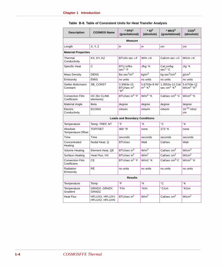
Table B-8. Table of Consistent Units for Heat Transfer Analysis
Description COSMOS Name * FPS1
(gravitational)* SI2
(absolute)* MKS3
(gravitational)CGS4
(absolute)
Measure
Length X, Y, Z in m cm cm
Material Properties
Thermal Conductivity
KX, KY, KZ BTU/in sec ∞F W/m ∞K Cal/cm sec ∞C W/cm ∞K
Specific Heat C BTU in/lbs sec2 °F
J/kg °K Cal cm/kg sec2 °C
J/g °K
Mass Density DENS lbs sec2/in4 kg/m3 kg sec2/cm4 g/cm3
Emissivity EMIS no units no units no units no units
Stefan Boltzmann Constant
SB_CONST 3.3063e-15 BTU/sec in2 °R4
5.6703e-8 W/m2 °K4
1.3552e-12 Cal/sec cm2 °K4
5.6703e-12 W/cm2 °K4
Convection Film Coefficient
HC (for CLINK elements)
BTU/sec in2 °F W/m2 °K Cal/sec cm2 °C W/cm2 °K
Material Angle Beta degree degree degree degree
Electric Conductivity
ECONX mho/in mho/m mho/m 10-13 mho/cm
Loads and Boundary Conditions
Temperature Temp, TREF, NT °F °K °C °K
Absolute Temperature Offset
TOFFSET 460 °R none 273 °K none
Time Time seconds seconds seconds seconds
Concentrated Heating
Nodal Heat, Q BTU/sec Watt Cal/sec Watt
Volume Heating Element Heat, QE BTU/sec in3 W/m3 Cal/sec cm3 W/cm3
Surface Heating Heat Flux, HX BTU/sec in2 W/m2 Cal/sec cm2 W/cm2
Convection Film Coefficient
CE BTU/sec in2 °F W/m2 °K Cal/sec cm2°C W/cm2 °K
Radiation Emissivity
RE no units no units no units no units
Results
Temperature Temp °F °K °C °K
Temperature Gradient
GRADX, GRADY, GRADZ
°F/in °K/m °C/cm °K/cm
Heat Flux HFLUXX, HFLUXY, HFLUXZ, HFLUXN
BTU/sec in2 W/m2 Cal/sec cm2 W/cm2
COSMOSFFE Thermal
2 Capabilities
Introduction
The following are some important features of COSMOSFFE Thermal.
Analysis Features
• Linear and nonlinear, steady-state and transient heat transfer
• Temperature-dependent material properties
• Time- and temperature-dependent heat sources and sinks
• Time- and temperature-dependent or heat flux, convection and radiation boundary conditions:
- Heat Flux
- Convection
- Radiation
• Time-dependent prescribed temperatures
• First and second order elements
• Heat Transfer - Structural coupling where resulting temperatures can be included in structural problems
• Restart option for transient problems
COSMOSFFE Thermal 2-1
Chapter 2 Capabilities
2-2
Internal Heat Generation
Internal heat generation can be applied to any node or element of the model.
Material properties
FFE Thermal supports isotropic materials. Orthotropic material properties, if defined, are always considered in the global coordinate system only.
Temperature- and Time-Dependent Properties
Temperature curves are used to specify the variation of material properties with temperature and they are also used to prescribe the variation of convection coefficient, heat generation rate, surface emissivity, and heat fluxes with temperature. Time curves are used to specify the variation of parameters such as convection, temperature, etc. with time.
Temperature-dependent convection coefficients are calculated based on the average film temperatures (Ts + T∞)/2. Temperature dependent emissivities or heat fluxes are calculated based on the surface temperature.
Thermal Stress Analysis
Once a thermal analysis is completed, resulting temperature distribution can be used to calculate thermal stresses in the material, using the FFEStatic or STAR.
Size Limits
Three variation of GEOSTAR are installed on your computer, the three variations support 64,000, 128,000,and 256,000 nodes and elements, respectively. Each variation may be started by double-clicking the corresponding icon in the COSMOSM 2.0 program group The limits represent the maximum node and
COSMOSFFE Thermal
Chapter 2 Capabilities
element labels that may be created in GEOSTAR. Please note that these variations are not compatible with each other. The session and neutral (gfm) files are however compatible.
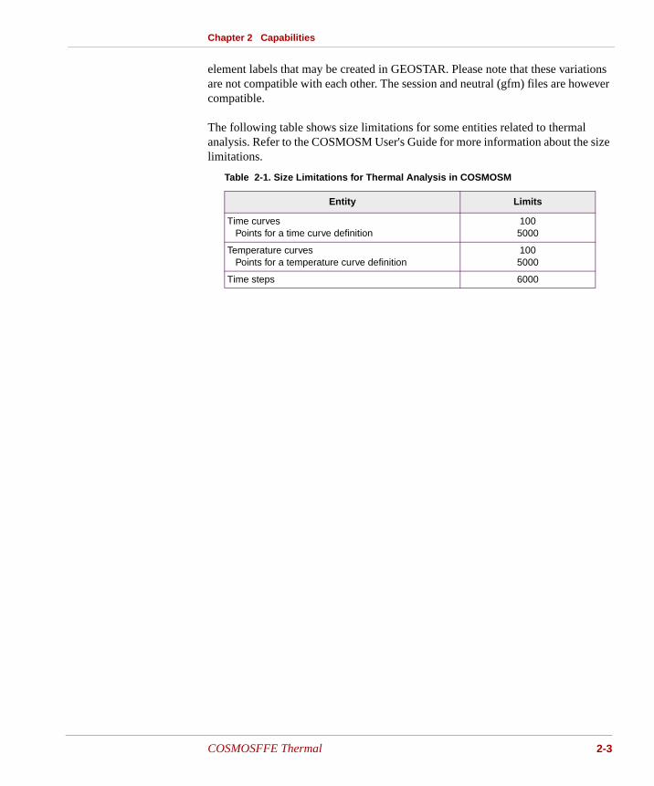
The following table shows size limitations for some entities related to thermal analysis. Refer to the COSMOSM User's Guide for more information about the size limitations.
Table 2-1. Size Limitations for Thermal Analysis in COSMOSM
Entity Limits
Time curves Points for a time curve definition
1005000
Temperature curves Points for a temperature curve definition
1005000
Time steps 6000
COSMOSFFE Thermal 2-3

2-4
COSMOSFFE Thermal
3 Element Library
Introduction
The COSMOSFFE Thermal module features an extensive element library to satisfy your finite element modeling and analysis requirements for all types of practical heat transfer problems. These elements model the behavior of 1D, 2D, and 3D problems in linear and nonlinear steady-state and transient heat transfer computations. The following table lists the elements available for analysis in the COSMOSFFE Thermal module.
Table 3-1. Elements for Thermal Analysis
Type Name Order
Two dimensional elastic beam element BEAM2D First
Three dimensional elastic beam element BEAM3D First
Convection link CLINK . . .
4/8-node plane and axisymmetric element PLANE2D First/Second
Radiation link RLINK . . .
3-node thin shell element SHELL3 First
3-node thick shell element SHELL3T First
4-node thin shell element SHELL4 First
4-node thick shell element SHELL4T First
8/20-node 3D solid element SOLID First/Second
COSMOSFFE Thermal 3-1
Chapter 3 Element Library
3-2
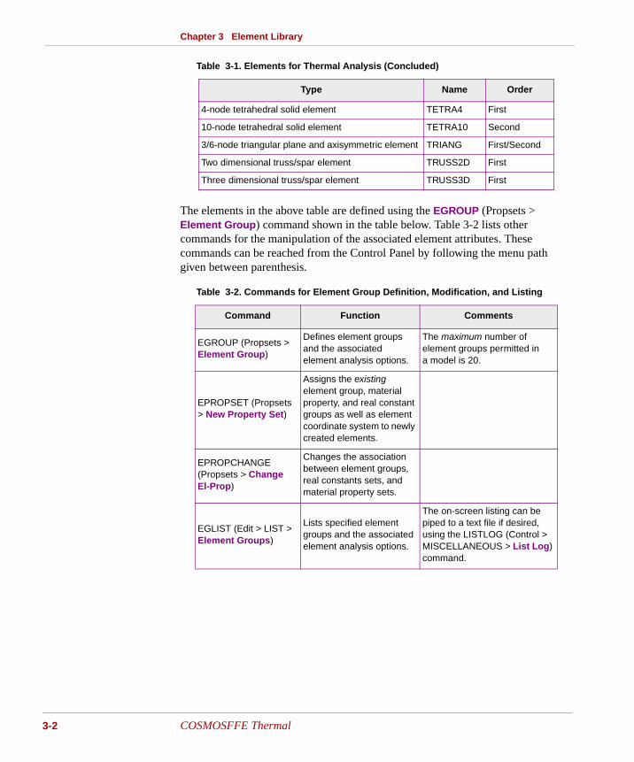
Table 3-1. Elements for Thermal Analysis (Concluded)
The elements in the above table are defined using the EGROUP (Propsets > Element Group) command shown in the table below. Table 3-2 lists other commands for the manipulation of the associated element attributes. These commands can be reached from the Control Panel by following the menu path given between parenthesis.
Table 3-2. Commands for Element Group Definition, Modification, and Listing
Type Name Order
4-node tetrahedral solid element TETRA4 First
10-node tetrahedral solid element TETRA10 Second
3/6-node triangular plane and axisymmetric element TRIANG First/Second
Two dimensional truss/spar element TRUSS2D First
Three dimensional truss/spar element TRUSS3D First
Command Function Comments
EGROUP (Propsets > Element Group)
Defines element groups and the associated element analysis options.
The maximum number of element groups permitted in a model is 20.
EPROPSET (Propsets > New Property Set)
Assigns the existing element group, material property, and real constant groups as well as element coordinate system to newly created elements.
EPROPCHANGE (Propsets > Change El-Prop)
Changes the association between element groups, real constants sets, and material property sets.
EGLIST (Edit > LIST > Element Groups)
Lists specified element groups and the associated element analysis options.
The on-screen listing can be piped to a text file if desired, using the LISTLOG (Control > MISCELLANEOUS > List Log) command.
COSMOSFFE Thermal
Chapter 3 Element Library
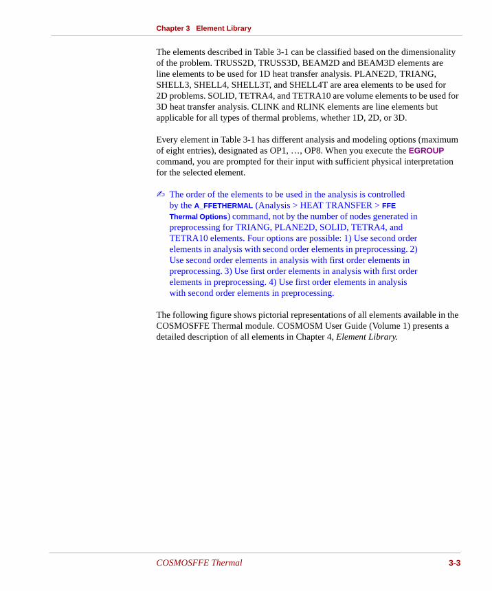
The elements described in Table 3-1 can be classified based on the dimensionality of the problem. TRUSS2D, TRUSS3D, BEAM2D and BEAM3D elements are line elements to be used for 1D heat transfer analysis. PLANE2D, TRIANG, SHELL3, SHELL4, SHELL3T, and SHELL4T are area elements to be used for 2D problems. SOLID, TETRA4, and TETRA10 are volume elements to be used for 3D heat transfer analysis. CLINK and RLINK elements are line elements but applicable for all types of thermal problems, whether 1D, 2D, or 3D.
Every element in Table 3-1 has different analysis and modeling options (maximum of eight entries), designated as OP1, …, OP8. When you execute the EGROUP command, you are prompted for their input with sufficient physical interpretation for the selected element.
✍ The order of the elements to be used in the analysis is controlled by the A_FFETHERMAL (Analysis > HEAT TRANSFER > FFE
Thermal Options) command, not by the number of nodes generated in preprocessing for TRIANG, PLANE2D, SOLID, TETRA4, and TETRA10 elements. Four options are possible: 1) Use second order elements in analysis with second order elements in preprocessing. 2) Use second order elements in analysis with first order elements in preprocessing. 3) Use first order elements in analysis with first order elements in preprocessing. 4) Use first order elements in analysis with second order elements in preprocessing.
The following figure shows pictorial representations of all elements available in the COSMOSFFE Thermal module. COSMOSM User Guide (Volume 1) presents a detailed description of all elements in Chapter 4, Element Library.
COSMOSFFE Thermal 3-3
Chapter 3 Element Library
3-4
Figure 3-1. Elements for Linear and Nonlinear Steady-State and Transient Heat Transfer Analyses
4-Node Plane or Axisymmetric QuadrilateralElement: PLANE2DNodes: 4
8-Node Plane or Axisymmetric QuadrilateralElement: PLANE2DNodes: 8
3-Node Plane or Axisymmetric TriangleElement: TRIANGNodes: 3
6-Node Plane or Axisymmetric TriangleElement: TRIANGNodes: 6
3-Node ShellElement: SHELL3 or SHELL3TNodes: 3
4-Node ShellElement: SHELL4 or SHELL4TNodes: 4
4-Node Tetrahedral SolidElement: TETRA4Nodes: 4
10-Node Tetrahedral SolidElement: TETRA10Nodes: 10
8-Node SolidElement: SOLIDNodes: 8
20-Node SolidElement: SOLIDNodes: 20
First OrderPrism-Shaped SolidElement: SOLIDNodes: 8 with a face collasping to an edge
Second Order Prism-Shaped SolidElement: SOLIDNodes: 20 with a face collasping to an edge
Truss/ SparElement: TRUSS2D or TRUSS3DNodes: 2
BeamElement: BEAM2D or BEAM3DNodes: 2 or 3
Convect ion LinkElement: CLINKNodes: 2 or 3
Radiat ion LinkElement: RLINKNodes: 2 or 3
COSMOSFFE Thermal

4 Input Data
Introduction
Proper modeling and analysis specifications are crucial to the success of any finite element analysis. Irrespective of the type of analysis, numerical solution using finite element analysis requires complete information on the model under consideration. The finite element model you submit for analysis must contain all the necessary data for each step of numerical simulation - geometry, elements, loads, boundary conditions, solution of system of equations, visualization and output of results, etc. This chapter attempts to conceptually illustrate the procedure for building a model for analysis using the COSMOSFFE Thermal module.
Since a major portion of the effort in building a finite element model is made in geometry creation and meshing, these topics will not be discussed here. The COSMOSM User Guide (Volume 1) presents in-depth information on the procedures for model building and postprocessing in GEOSTAR. This chapter therefore only outlines those commands which are relevant for analysis in the COSMOSFFE Thermal module.
✍ For a detailed description of all commands, refer to the COSMOSM Command Reference Manual (Volume 2).
COSMOSFFE Thermal 4-1
Chapter 4 Input Data
4-2
Modeling and Analysis Cycle in the COSMOSFFE Thermal Module
The basic steps involved in a finite element analysis are:
• Create the problem geometry.
• Mesh the defined geometry with appropriate type of element(s).
• Apply constraints on the finite element model.
• Define the loads on the model.
• Define the material and sectional properties.
• Submit the completed finite element model for analysis.
• Interpret and analyze the results.
These steps can be schematically represented as shown in the figure below.
Figure 4-1. Finite Element Modeling and Analysis Steps
Preprocessing refers to the operations you perform such as defining the model geometry, mesh generation, applying loads and boundary conditions, and other operations that are required prior to submitting the model for analysis. The term analysis in the above figure refers to the phase of specifying the analysis options and executing the actual analysis. Postprocessing refers to the manipulation of the analysis results for easy understanding and interpretation in a graphical environment.
The commands summarized in the table below provide you with information on the input of element groups, material and sectional properties, loads and boundary conditions, analysis specifications, and output specifications.
START
PREPROCESSING POSTPROCESSING
STOPAnalysis and
Design DecisionsProblem Definition
ANALYSIS
COSMOSFFE Thermal
Chapter 4 Input Data
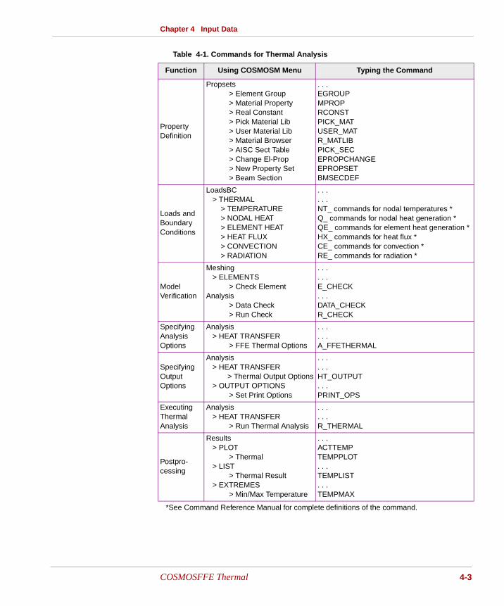
Table 4-1. Commands for Thermal Analysis
Function Using COSMOSM Menu Typing the Command
Property Definition
Propsets > Element Group > Material Property > Real Constant > Pick Material Lib > User Material Lib > Material Browser > AISC Sect Table > Change El-Prop > New Property Set > Beam Section
. . .EGROUPMPROPRCONSTPICK_MATUSER_MATR_MATLIBPICK_SECEPROPCHANGEEPROPSETBMSECDEF
Loads and Boundary Conditions
LoadsBC > THERMAL > TEMPERATURE > NODAL HEAT > ELEMENT HEAT > HEAT FLUX > CONVECTION > RADIATION
. . .
. . .NT_ commands for nodal temperatures *Q_ commands for nodal heat generation *QE_ commands for element heat generation *HX_ commands for heat flux *CE_ commands for convection *RE_ commands for radiation *
Model Verification
Meshing > ELEMENTS > Check ElementAnalysis > Data Check > Run Check
. . .
. . .E_CHECK. . .DATA_CHECKR_CHECK
Specifying Analysis Options
Analysis > HEAT TRANSFER > FFE Thermal Options
. . .
. . .A_FFETHERMAL
Specifying Output Options
Analysis > HEAT TRANSFER > Thermal Output Options > OUTPUT OPTIONS > Set Print Options
. . .
. . .HT_OUTPUT. . .PRINT_OPS
Executing Thermal Analysis
Analysis > HEAT TRANSFER > Run Thermal Analysis
. . .
. . .R_THERMAL
Postpro-cessing
Results > PLOT > Thermal > LIST > Thermal Result > EXTREMES > Min/Max Temperature
. . .ACTTEMPTEMPPLOT. . .TEMPLIST. . .TEMPMAX
*See Command Reference Manual for complete definitions of the command.
COSMOSFFE Thermal 4-3

Chapter 4 Input Data
4-4
Temperature and Time Curves
Temperature and time curves are used to specify the variation of temperature and time dependent properties, respectively. Using a time or temperature curve involves the following steps.
• Define the temperature or time curve using the CURDEF (LoadsBC > FUNCTION CURVE > Time/Temp Curve) command. The created curve is automatically activated.
• Define the entity of interest (boundary condition, load, material property etc.).
• Deactivate the curve using ACTSET (Control > ACTIVATE > Set Entity) command so that this curve is not inadvertently associated with some other entity defined later on.
For example, prescription of a temperature varying thermal conductivity may be done as follows. Issue the CURDEF (LoadsBC > FUNCTION CURVE > Time/Temp Curve) command to define temperature curve number 1 and then issue the following sequence of commands:
Geo Panel: Control > ACTIVATE > Set Entity
Set Label > Temperature Curve
Click on Continue icon
Load case set number > 1Accept entries
Geo Panel: Propsets > Material Property
Material Property Set [1] >Material Property Name > XThermal Conductivity Property value [0.0] > 1.0
Accept all entries
Geo Panel: Control > ACTIVATE > Set Entity
Set Label > Temperature Curve
Click on Continue icon
Load case set number > 0Accept entries
COSMOSFFE Thermal
Chapter 4 Input Data
Thermal Stress Analysis
Once a thermal analysis is completed, resulting temperature profiles can be used to calculate corresponding thermal stresses. The following steps can be used to calculate thermal stresses:
• Complete the thermal analysis.
• Use TEMPREAD (LoadsBC > LOAD OPTIONS > Read Temp as Load) command to assign the heat transfer results at a specific time step to a specific load case for stress computation. Repeat the TEMPREAD command to assign time steps to different load cases if desired.
• Activate thermal loading using the A_FFESTATIC (Analysis > STATIC > FFE Static Options) command.
• Run the static analysis using R_STATIC (Analysis > STATIC > Run Static Analysis) command.
Thermal Analysis Options
The A_FFETHERMAL Command
Geo Panel: Analysis > HEAT TRANSFER > FFE Thermal Options
The A_FFETHERMAL (Analysis > HEAT TRANSFER > FFE Thermal Options) command specifies analysis options for heat transfer analysis using the FFE Thermal module. Note that the A_THERMAL (Analysis > HEAT TRANSFER > Thermal Analysis Options) command specifies analysis options for heat transfer analysis using the HSTAR module.
Entry & Option Description
analysis-option
Type of analysis to be performed.
S Steady-stateT Transient
(default is S)
element-order
Order of the element to be used. In spite of the element group name in the data-base, you may specify through this option whether first (linear) or second (para-bolic) elements will be used. As an example, if you define TETRA4 elements and use second order, middle nodes on straight edges will be considered during
COSMOSFFE Thermal 4-5
Chapter 4 Input Data
4-6
analysis. On the other hand you may define TETRA10 elements and specify to use first order. SOLID elements are treated similarly except that for these ele-ments the same element group names are used for both first and second orders.
1 Use first order elements2 Use second order elements
(default is 2)
tolerance
Convergence tolerance for nonlinear problems.(default is 0.001)
unused-option
Unused option preserved for backward compatibility only.
mass-form
Mass matrix formulation used for transient analysis. It also affects matrix-for-mulation for convection and radiation.
1 Lumped (ignored if selected with second order elements)2 Consistent
(default is 1)
Running Thermal Analysis
The R_THERMAL (Analysis > HEAT TRANSFER > Run Thermal Analysis) command performs thermal analysis using HSTAR or FFE Thermal. The command runs the conventional HSTAR or the FFE Thermal module depending on the option specified by the A_FFETHERMAL or the A_THERMAL commands. The command will run the HSTAR module if none of the commands have been issued.
Postprocessing
The output generated by the thermal analysis can be viewed graphically in GEOSTAR. From the Geo Panel, select Results > PLOT > Thermal in order to have a contour plot of temperature, gradient or heat flux. An option menu will appear on the screen to specify the plotting options. Note that if the user preferred to type the command using the keyboard, two commands would have been used, namely, ACTTEMP and TEMPLOT commands. You may also look at the time history of temperature, gradient, etc. at any node. First issue the ACTXYPLOT (Display > XY PLOTS > Activate Post-Proc) to load the proper data into memory and then issue XYPLOT (Display > XY PLOTS > Plot Curves) to plot the time history of the selected item.
COSMOSFFE Thermal
Chapter 4 Input Data
Verification of Model Input Data
One of the difficulties you may come across in the solution of small or large problems alike is avoiding errors in the model input data. Some of the errors can be detected by plotting the model in various positions, listing the element connectivities, listing material and sectional properties, plotting or listing loads and constraints, and many other on-line tools. For small problems, it is often easier to perform these checks to see if all required input data have been properly generated and defined. However, you may still miss some errors that are not easily identifiable. For these types of situations and also for larger problems, it is plausible to perform model checks in an automated environment. COSMOSFFE provides powerful tools to automatically verify the robustness and validity of the finite element model you build within GEOSTAR. The table below shows the commands you can use in model verification and their functions.
Table 4-2. Commands for Model Input Verification
As you can notice from the above table, the DATA_CHECK command is a subset of the R_CHECK command. Even though the R_CHECK command identifies elements with bad geometry, the deletion of degenerate elements is performed by the ECHECK command.
✍ You are strongly recommended to use the R_CHECK command and apply any corrections to the finite element model before performing any analysis.
Note that the R_CHECK command is a general model verification tool. You may still find some errors that are not trapped by the use of this command. In most cases, the diagnostic messages either printed on the screen or written to an ASCII file (*.CHK) provide further information as to the nature of error and its remedies.
Using the MenuTyping the Command
Function
Meshing > ELEMENTS > Check Element
ECHECK
Checks the aspect ratios of specified elements. The command automatically deletes the degenerate elements from the model. The command also checks the element connectivities.
Analysis > Data Check
DATA_CHECKChecks if an element group, material property set, and a real (section) constant have been defined for each element in the model.
Analysis > Run Check
R_CHECKPerforms rigorous checks on the model for validity and completeness for the specified type of analysis.
COSMOSFFE Thermal 4-7

4-8
COSMOSFFE Thermal
5 Examples
Introduction
This chapter presents detailed examples for performing linear and nonlinear heat transfer analysis using the COSMOSFFE Thermal module. The examples discussed include large size practical problems as well as those of academic type for verification purposes. Some benchmark results are also provided to demonstrate the savings obtained in solution time and resources.
The following are some hints to assist you in performing a heat transfer analysis using the COSMOSFFE Thermal module:
• The A_FFETHERMAL (Analysis > HEAT TRANSFER > FFE Thermal Options) command controls options of subsequent thermal analysis using the FFE Thermal module. The A_THERMAL (Analysis > HEAT TRANSFER > Thermal Analysis Options) command controls options to be used by HSTAR, the conventional heat transfer analysis module of COSMOSM.
• If you are using the existing COSMOSM HSTAR input files for analysis in COSMOSFFE Thermal, you need to use the A_FFETHERMAL command to specify analysis options.
• Information about used resources and the analysis module's messages are written to an output file with .OUT extension.
• The RESTART (Analysis > Restart) command controls the restart option for transient analysis.
COSMOSFFE Thermal 5-1
Chapter 5 Examples
5-2
Example Problems
Four examples are presented in the following pages. The first example discusses steady-state linear heat transfer analysis using four different types of elements. The second example deals with steady-state nonlinear heat transfer analysis due to radiating boundary conditions. The next two examples represent problems with large number of degrees of freedom to demonstrate the efficiency of COSMOSFFE.
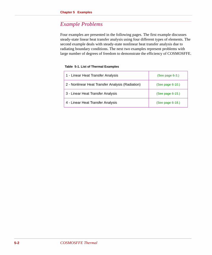
Table 5-1. List of Thermal Examples
1 - Linear Heat Transfer Analysis (See page 6-3.)
2 - Nonlinear Heat Transfer Analysis (Radiation) (See page 6-10.)
3 - Linear Heat Transfer Analysis (See page 6-15.)
4 - Linear Heat Transfer Analysis (See page 6-18.)
COSMOSFFE Thermal
Chapter 5 Examples
See age -2.)
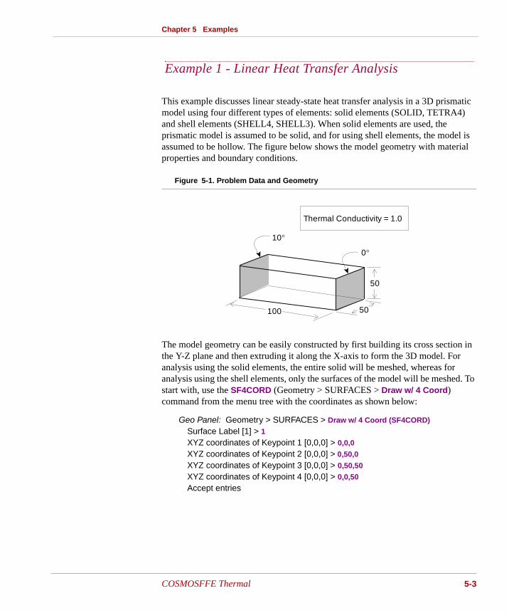
This example discusses linear steady-state heat transfer analysis in a 3D prismatic model using four different types of elements: solid elements (SOLID, TETRA4) and shell elements (SHELL4, SHELL3). When solid elements are used, the prismatic model is assumed to be solid, and for using shell elements, the model is assumed to be hollow. The figure below shows the model geometry with material properties and boundary conditions.
Figure 5-1. Problem Data and Geometry
The model geometry can be easily constructed by first building its cross section in the Y-Z plane and then extruding it along the X-axis to form the 3D model. For analysis using the solid elements, the entire solid will be meshed, whereas for analysis using the shell elements, only the surfaces of the model will be meshed. To start with, use the SF4CORD (Geometry > SURFACES > Draw w/ 4 Coord) command from the menu tree with the coordinates as shown below:
Geo Panel: Geometry > SURFACES > Draw w/ 4 Coord (SF4CORD)
Surface Label [1] > 1XYZ coordinates of Keypoint 1 [0,0,0] > 0,0,0
XYZ coordinates of Keypoint 2 [0,0,0] > 0,50,0
XYZ coordinates of Keypoint 3 [0,0,0] > 0,50,50
XYZ coordinates of Keypoint 4 [0,0,0] > 0,0,50
Accept entries
Example 1 - Linear Heat Transfer Analysis (p6
Thermal Conductivity = 1.0
0°
10°
50
100 50
COSMOSFFE Thermal 5-3
Chapter 5 Examples
5-4
Next, use the VLEXTR (Geometry > VOLUMES > GENERATION MENU > Extrusion) command to extrude the cross section along the X-axis as illustrated below:
Geo Panel: Geometry > VOLUMES > GENERATION MENU > Extrusion (VLEXTR)
Beginning Surface > 1Ending Surface [1] >Increment [1] >Axis symbol [Z] > XValue > 100
Accept entries
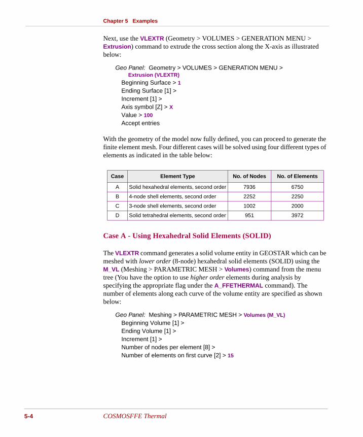
With the geometry of the model now fully defined, you can proceed to generate the finite element mesh. Four different cases will be solved using four different types of elements as indicated in the table below:
Case A - Using Hexahedral Solid Elements (SOLID)
The VLEXTR command generates a solid volume entity in GEOSTAR which can be meshed with lower order (8-node) hexahedral solid elements (SOLID) using the M_VL (Meshing > PARAMETRIC MESH > Volumes) command from the menu tree (You have the option to use higher order elements during analysis by specifying the appropriate flag under the A_FFETHERMAL command). The number of elements along each curve of the volume entity are specified as shown below:
Geo Panel: Meshing > PARAMETRIC MESH > Volumes (M_VL)
Beginning Volume [1] >Ending Volume [1] >Increment [1] >Number of nodes per element [8] >Number of elements on first curve [2] > 15
Case Element Type No. of Nodes No. of Elements
A Solid hexahedral elements, second order 7936 6750
B 4-node shell elements, second order 2252 2250
C 3-node shell elements, second order 1002 2000
D Solid tetrahedral elements, second order 951 3972
COSMOSFFE Thermal
Chapter 5 Examples
Number of elements on second curve [2] > 15
Number of elements on third curve [2] > 30
Accept all default values
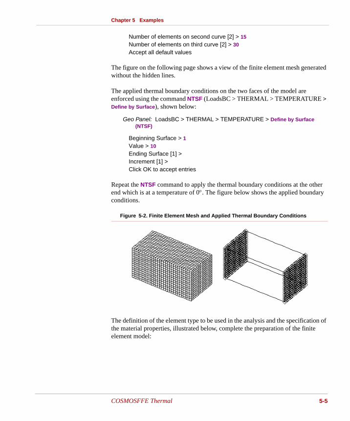
The figure on the following page shows a view of the finite element mesh generated without the hidden lines.
The applied thermal boundary conditions on the two faces of the model are enforced using the command NTSF (LoadsBC > THERMAL > TEMPERATURE > Define by Surface), shown below:
Geo Panel: LoadsBC > THERMAL > TEMPERATURE > Define by Surface (NTSF)
Beginning Surface > 1Value > 10
Ending Surface [1] >Increment [1] >Click OK to accept entries
Repeat the NTSF command to apply the thermal boundary conditions at the other end which is at a temperature of 0°. The figure below shows the applied boundary conditions.
Figure 5-2. Finite Element Mesh and Applied Thermal Boundary Conditions
The definition of the element type to be used in the analysis and the specification of the material properties, illustrated below, complete the preparation of the finite element model:
COSMOSFFE Thermal 5-5
Chapter 5 Examples
5-6
Geo Panel: Propsets > Element Group (EGROUP)
Element group set label [1] > 1Element Name > SOLID
Click on Continue icon
Accept all default entries
Geo Panel: Propsets > Material Property (MPROP)
Material property set [1] > 1Material property name > KX
Property value > 1.0
Click on OK icon
Click Cancel to end this command
Before proceeding to perform the heat transfer analysis, you need to specify the appropriate flags for analysis using the A_FFETHERMAL (Analysis > HEAT TRANSFER > FFE Thermal Options) command as illustrated below:
Geo Panel: Analysis > HEAT TRANSFER > FFE Thermal Options (A_FFETHERMAL)
Analysis option [S: Steady] >Element order 1=First 2=Second [2] >Convergence tolerance [0.001] >Unused option >Formulation flag 0=lump 1=cons >Click OK to accept entries
The options selected above specify steady state heat transfer analysis using second order elements. The command R_THERMAL (Analysis > HEAT TRANSFER > Run Thermal Analysis) can now be used to execute analysis. After successful completion of analysis, you can proceed to postprocess the results.
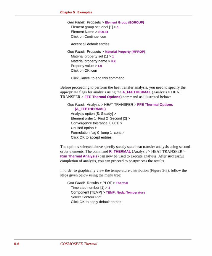
In order to graphically view the temperature distribution (Figure 5-3), follow the steps given below using the menu tree:
Geo Panel: Results > PLOT > Thermal
Time step number [1] > 1Component [TEMP] > TEMP: Nodal Temperature
Select Contour PlotClick OK to apply default entries
COSMOSFFE Thermal
Chapter 5 Examples
If the user preferred to type in the commands using the keyboard, two commands should be typed in:
GEO > ACTTEMP;
GEO > TEMPLOT;
Figure 5-3. Temperature Contour Plot
The solution time data for the problem can be obtained from the output file (jobname.OUT).
Case B - Using Quadrilateral Shell Elements (SHELL4)
Delete the mesh using the command MVLDEL (Edit > DELETE > Element on Volume) and select the M_SF (Meshing > PARAMETRIC MESH > Surfaces) command to mesh only the surfaces of the model. To begin with, select the end faces (surfaces 1 and 2), and in the second attempt, select the side faces (surfaces 3 through 6). For the end faces, specify the number of elements as 15 along each curve. For the side faces, specify 15 elements along the shorter curve, and 30 elements along the longer curve. When you are meshing these surfaces, specify
COSMOSFFE Thermal 5-7
Chapter 5 Examples
5-8
lower order elements (4-noded elements in this case). Since the mesh is generated independently for each surface, you need to use the NMERGE (Meshing > NODES > Merge) and NCOMPRESS (Edit > Compress Nodes) commands from the menu tree to merge the nodes and remove node numbering gaps respectively, in order to satisfy the compatibility requirements.
You need to redefine the element group, specifying SHELL4 with default options. You also need to specify a thickness of 0.1 for this element using the RCONST (Propsets > Real Constant) command with entries shown below:
Geo Panel: Propsets > Element Group
EGROUP,1,SHELL4;
Geo Panel: Propsets > Real Constant
RCONST,1,1,1,6,0.1;
Use the NTSF command as before to apply the thermal boundary conditions at the two end faces. The analysis options set by the A_FFETHERMAL command still remain valid, with second order solutions specified for this case also. The command R_THERMAL can now be used to execute the analysis. As before, you can view the temperature contour plot. You will notice that the contours are the same as those obtained using solid hexahedral elements.
Case C - Using Triangular Shell Elements (SHELL3)
Delete the mesh using the command MSFDEL (Edit > DELETE > Element on Surface). We will use the 3D automatic meshing feature for polyhedron in this case. From the Geometry > POLYHEDRA menu tree, select the Define (PH) command and generate a polyhedron out of the available surfaces as follows:
Geo Panel: Geometry > POLYHEDRA > Define (PH)
Label of polyhedron [1] > 1Reference entity name [RG] > SF
Then acceptSurface label [1] > 1Average element size > 5Accept all entries
Next, from the Meshing > AUTO MESH menu tree, select the Polyhedra (MA_PH) command to generate a mesh of triangular elements. This command by default generates lower order elements.
COSMOSFFE Thermal
Chapter 5 Examples
You also need to redefine the element group, specifying SHELL3 with default options. You need to specify a thickness of 0.1 using the RCONST command as used before.
EGROUP,1,SHELL3;
RCONST,1,1,1,6,0.1;
Use the NTSF command as before to apply the thermal boundary conditions at the two end faces. The analysis options set by the A_FFETHERMAL command still remain valid, with second order solutions specified for this case also. The command R_THERMAL can now be used to execute analysis. As before, you can view the temperature contour plot.
Case D - Using Tetrahedral Solid Elements (TETRA4)
Delete the mesh using the command MSFDEL (Edit > DELETE > Element on Surface) from the menu tree. We will use the 3D automatic meshing feature for part entities in this case. From the Edit > DELETE menu tree, select the Polyhedra (PHDEL) command and delete the polyhedron defined earlier. Re-execute the PH command and specify an average element size of 7.5. Alternately, you can use the PHDENSITY (Meshing > MESH DENSITY > Polyhedron Elem Size) command to redefine the mesh density of a polyhedron. To define a solid entity, you need to use the PART (Geometry > Define Part) command. Next, from the Meshing > AUTO MESH menu tree, select the command Parts (MA_PART) to generate a mesh of tetrahedral elements.
You also need to redefine the element group, specifying TETRA4 with default options.
EGROUP,1,TETRA4;
Use the NTSF command as before to apply the thermal boundary conditions at the two end faces. The analysis options set by the A_FFETHERMAL command still remain valid, with second order solutions specified for this case also. The command R_THERMAL can now be used to execute analysis. As before, you can view the temperature contour plot.
COSMOSFFE Thermal 5-9
Chapter 5 Examples
5-10
See age -2.)
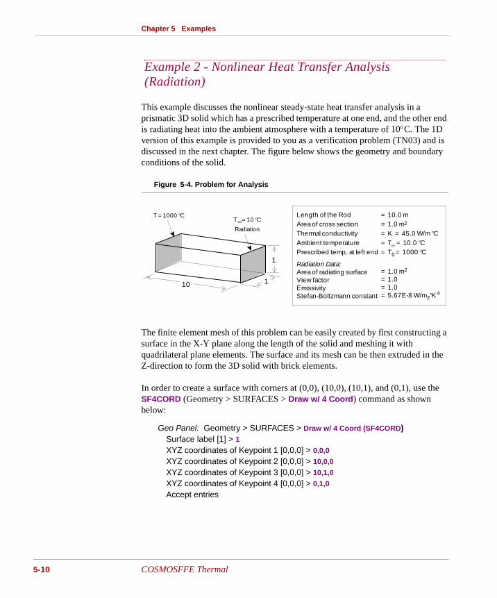
This example discusses the nonlinear steady-state heat transfer analysis in a prismatic 3D solid which has a prescribed temperature at one end, and the other end is radiating heat into the ambient atmosphere with a temperature of 10°C. The 1D version of this example is provided to you as a verification problem (TN03) and is discussed in the next chapter. The figure below shows the geometry and boundary conditions of the solid.
Figure 5-4. Problem for Analysis
The finite element mesh of this problem can be easily created by first constructing a surface in the X-Y plane along the length of the solid and meshing it with quadrilateral plane elements. The surface and its mesh can be then extruded in the Z-direction to form the 3D solid with brick elements.
In order to create a surface with corners at (0,0), (10,0), (10,1), and (0,1), use the SF4CORD (Geometry > SURFACES > Draw w/ 4 Coord) command as shown below:
Geo Panel: Geometry > SURFACES > Draw w/ 4 Coord (SF4CORD)Surface label [1] > 1XYZ coordinates of Keypoint 1 [0,0,0] > 0,0,0
XYZ coordinates of Keypoint 2 [0,0,0] > 10,0,0
XYZ coordinates of Keypoint 3 [0,0,0] > 10,1,0
XYZ coordinates of Keypoint 4 [0,0,0] > 0,1,0
Accept entries
Example 2 - Nonlinear Heat Transfer Analysis (Radiation)
(p6
Length of the Rod Area of cross section Thermal conductivity Ambient temperature Prescribed temp. at left end
= 10.0 m= 1.0 m= K = 45.0 W/m °C= T = 10.0 °C= T = 1000 °C
Radiation Data:Area of radiating surface View factor Emissivity Stefan-Boltzmann constant
= 1.0 m= 1.0= 1.0= 5.67E-8 W/m °K
0
∞
24
2
2
T = 1000 °CT = 10 °C∞ Radiation
1
10 1
COSMOSFFE Thermal
Chapter 5 Examples
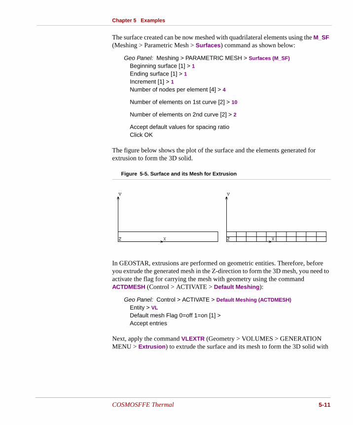
The surface created can be now meshed with quadrilateral elements using the M_SF (Meshing > Parametric Mesh > Surfaces) command as shown below:
Geo Panel: Meshing > PARAMETRIC MESH > Surfaces (M_SF)
Beginning surface [1] > 1Ending surface [1] > 1Increment [1] > 1Number of nodes per element [4] > 4
Number of elements on 1st curve [2] > 10
Number of elements on 2nd curve [2] > 2
Accept default values for spacing ratioClick OK
The figure below shows the plot of the surface and the elements generated for extrusion to form the 3D solid.
Figure 5-5. Surface and its Mesh for Extrusion
In GEOSTAR, extrusions are performed on geometric entities. Therefore, before you extrude the generated mesh in the Z-direction to form the 3D mesh, you need to activate the flag for carrying the mesh with geometry using the command ACTDMESH (Control > ACTIVATE > Default Meshing):
Geo Panel: Control > ACTIVATE > Default Meshing (ACTDMESH)
Entity > VL
Default mesh Flag 0=off 1=on [1] >Accept entries
Next, apply the command VLEXTR (Geometry > VOLUMES > GENERATION MENU > Extrusion) to extrude the surface and its mesh to form the 3D solid with
COSMOSFFE Thermal 5-11
Chapter 5 Examples
5-12
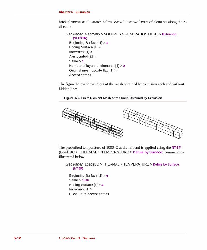
brick elements as illustrated below. We will use two layers of elements along the Z-direction.
Geo Panel: Geometry > VOLUMES > GENERATION MENU > Extrusion (VLEXTR)
Beginning Surface [1] > 1Ending Surface [1] > Increment [1] >Axis symbol [Z] >Value > 1Number of layers of elements [4] > 2Original mesh update flag [1] > Accept entries
The figure below shows plots of the mesh obtained by extrusion with and without hidden lines.
Figure 5-6. Finite Element Mesh of the Solid Obtained by Extrusion
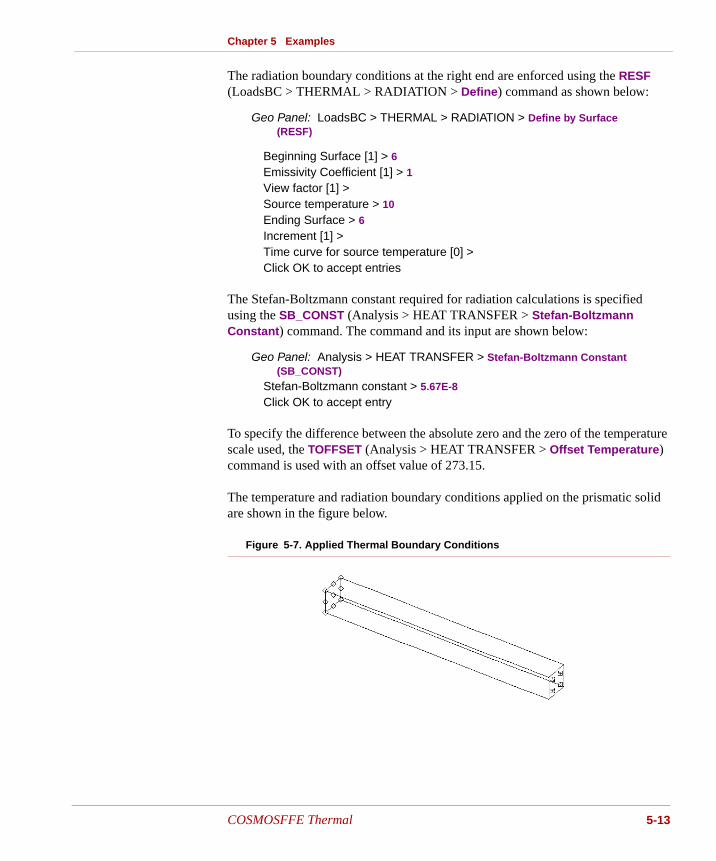
The prescribed temperature of 1000°C at the left end is applied using the NTSF (LoadsBC > THERMAL > TEMPERATURE > Define by Surface) command as illustrated below:
Geo Panel: LoadsBC > THERMAL > TEMPERATURE > Define by Surface (NTSF)
Beginning Surface [1] > 4Value > 1000
Ending Surface [1] > 4Increment [1] > Click OK to accept entries
COSMOSFFE Thermal
Chapter 5 Examples
The radiation boundary conditions at the right end are enforced using the RESF (LoadsBC > THERMAL > RADIATION > Define) command as shown below:
Geo Panel: LoadsBC > THERMAL > RADIATION > Define by Surface (RESF)
Beginning Surface [1] > 6Emissivity Coefficient [1] > 1View factor [1] > Source temperature > 10
Ending Surface > 6Increment [1] > Time curve for source temperature [0] > Click OK to accept entries
The Stefan-Boltzmann constant required for radiation calculations is specified using the SB_CONST (Analysis > HEAT TRANSFER > Stefan-Boltzmann Constant) command. The command and its input are shown below:
Geo Panel: Analysis > HEAT TRANSFER > Stefan-Boltzmann Constant (SB_CONST)
Stefan-Boltzmann constant > 5.67E-8
Click OK to accept entry
To specify the difference between the absolute zero and the zero of the temperature scale used, the TOFFSET (Analysis > HEAT TRANSFER > Offset Temperature) command is used with an offset value of 273.15.
The temperature and radiation boundary conditions applied on the prismatic solid are shown in the figure below.
Figure 5-7. Applied Thermal Boundary Conditions
COSMOSFFE Thermal 5-13
Chapter 5 Examples
5-14
The definition of the element type to be used in the analysis and the specification of the material properties, illustrated below, are defined using the Propsets menu tree to complete the preparation of the finite element model:
EGROUP,1,SOLID;
MPROP,1,KX,45;
Before proceeding to perform the heat transfer analysis, you need to specify the appropriate flags for analysis using the A_FFETHERMAL (Analysis > HEAT TRANSFER > FFE Thermal Options) command with default entries.
The command R_THERMAL (Analysis > HEAT TRANSFER > Run Thermal
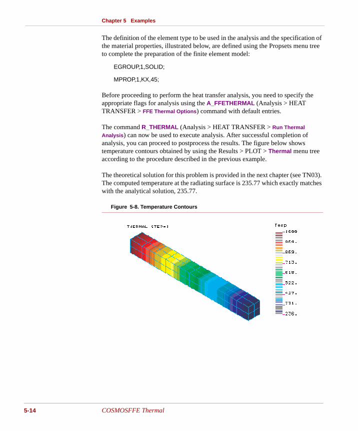
Analysis) can now be used to execute analysis. After successful completion of analysis, you can proceed to postprocess the results. The figure below shows temperature contours obtained by using the Results > PLOT > Thermal menu tree according to the procedure described in the previous example.
The theoretical solution for this problem is provided in the next chapter (see TN03). The computed temperature at the radiating surface is 235.77 which exactly matches with the analytical solution, 235.77.
Figure 5-8. Temperature Contours
COSMOSFFE Thermal
Chapter 5 Examples
See age -2.)
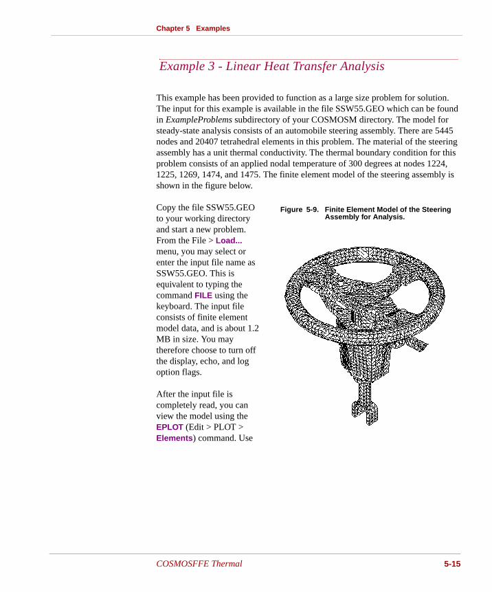
This example has been provided to function as a large size problem for solution. The input for this example is available in the file SSW55.GEO which can be found in ExampleProblems subdirectory of your COSMOSM directory. The model for steady-state analysis consists of an automobile steering assembly. There are 5445 nodes and 20407 tetrahedral elements in this problem. The material of the steering assembly has a unit thermal conductivity. The thermal boundary condition for this problem consists of an applied nodal temperature of 300 degrees at nodes 1224, 1225, 1269, 1474, and 1475. The finite element model of the steering assembly is shown in the figure below.
Copy the file SSW55.GEO to your working directory and start a new problem. From the File > Load... menu, you may select or enter the input file name as SSW55.GEO. This is equivalent to typing the command FILE using the keyboard. The input file consists of finite element model data, and is about 1.2 MB in size. You may therefore choose to turn off the display, echo, and log option flags.
After the input file is completely read, you can view the model using the EPLOT (Edit > PLOT > Elements) command. Use
Example 3 - Linear Heat Transfer Analysis (p6
Figure 5-9. Finite Element Model of the Steering Assembly for Analysis.
COSMOSFFE Thermal 5-15
Chapter 5 Examples
5-16
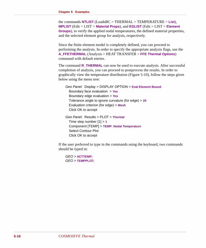
the commands NTLIST (LoadsBC > THERMAL > TEMPERATURE > List), MPLIST (Edit > LIST > Material Props), and EGLIST (Edit > LIST > Element Groups), to verify the applied nodal temperatures, the defined material properties, and the selected element group for analysis, respectively.
Since the finite element model is completely defined, you can proceed to performing the analysis. In order to specify the appropriate analysis flags, use the A_FFETHERMAL (Analysis > HEAT TRANSFER > FFE Thermal Options) command with default entries.
The command R_THERMAL can now be used to execute analysis. After successful completion of analysis, you can proceed to postprocess the results. In order to graphically view the temperature distribution (Figure 5-10), follow the steps given below using the menu tree:
Geo Panel: Display > DISPLAY OPTION > Eval Element Bound
Boundary face evaluation > Yes
Boundary edge evaluation > Yes
Tolerance angle to ignore curvature (for edge) > 20
Evaluation criterion (for edge) > Mesh
Click OK to accept
Geo Panel: Results > PLOT > Thermal
Time step number [1] > 1Component [TEMP] > TEMP: Nodal Temperature
Select Contour PlotClick OK to accept
If the user preferred to type in the commands using the keyboard, two commands should be typed in:
GEO > ACTTEMP;GEO > TEMPPLOT;
COSMOSFFE Thermal

Chapter 5 Examples
Figure 5-10. Temperature Contours
COSMOSFFE Thermal 5-17
Chapter 5 Examples
5-18
See age -2.)
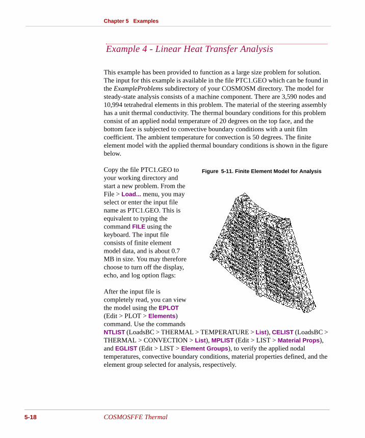
This example has been provided to function as a large size problem for solution. The input for this example is available in the file PTC1.GEO which can be found in the ExampleProblems subdirectory of your COSMOSM directory. The model for steady-state analysis consists of a machine component. There are 3,590 nodes and 10,994 tetrahedral elements in this problem. The material of the steering assembly has a unit thermal conductivity. The thermal boundary conditions for this problem consist of an applied nodal temperature of 20 degrees on the top face, and the bottom face is subjected to convective boundary conditions with a unit film coefficient. The ambient temperature for convection is 50 degrees. The finite element model with the applied thermal boundary conditions is shown in the figure below.
Copy the file PTC1.GEO to your working directory and start a new problem. From the File > Load... menu, you may select or enter the input file name as PTC1.GEO. This is equivalent to typing the command FILE using the keyboard. The input file consists of finite element model data, and is about 0.7 MB in size. You may therefore choose to turn off the display, echo, and log option flags:
After the input file is completely read, you can view the model using the EPLOT (Edit > PLOT > Elements) command. Use the commands NTLIST (LoadsBC > THERMAL > TEMPERATURE > List), CELIST (LoadsBC > THERMAL > CONVECTION > List), MPLIST (Edit > LIST > Material Props), and EGLIST (Edit > LIST > Element Groups), to verify the applied nodal temperatures, convective boundary conditions, material properties defined, and the element group selected for analysis, respectively.
Example 4 - Linear Heat Transfer Analysis (p6
Figure 5-11. Finite Element Model for Analysis
COSMOSFFE Thermal
Chapter 5 Examples
Since the finite element model is completely defined, you can proceed to performing the analysis. In order to specify the appropriate analysis flags, use the A_FFETHERMAL (Analysis > HEAT TRANSFER > FFE Thermal Options) command with default entries.
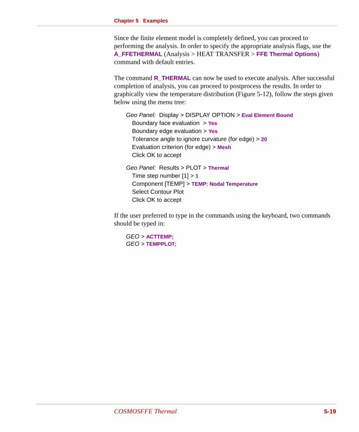
The command R_THERMAL can now be used to execute analysis. After successful completion of analysis, you can proceed to postprocess the results. In order to graphically view the temperature distribution (Figure 5-12), follow the steps given below using the menu tree:
Geo Panel: Display > DISPLAY OPTION > Eval Element Bound
Boundary face evaluation > Yes
Boundary edge evaluation > Yes
Tolerance angle to ignore curvature (for edge) > 20
Evaluation criterion (for edge) > Mesh
Click OK to accept
Geo Panel: Results > PLOT > Thermal
Time step number [1] > 1Component [TEMP] > TEMP: Nodal Temperature
Select Contour PlotClick OK to accept
If the user preferred to type in the commands using the keyboard, two commands should be typed in:
GEO > ACTTEMP;GEO > TEMPPLOT;
COSMOSFFE Thermal 5-19
Chapter 5 Examples
5-20
Figure 5-12. Temperature Contours
COSMOSFFE Thermal

6 Verification Problems
Introduction
In the following, a comprehensive set of benchmark problems are provided to illustrate the various features of the COSMOSFFE heat transfer analysis module. The problems are carefully selected to cover a wide range of applications in the field of thermal analysis.
The input files for FFE problems are available in “...\Vprobs\FFE” folder in the COSMOS installation directory. Where “...” refers to the directory in which you installed COSMOSM. You may copy the desired input file into your working directory, create a new problem, and then use the File (File > Load...) command to read the input file and to run the problem.
COSMOSFFE Thermal 6-1
Chapter 6 Verification Problems
6-2
Table 6-1. List of Verification Problems
Problem Element Title
FFETL01 SHELL3T Steady State Heat Conduction in a Square Plate (See page 6-3.)
FFETL02 SHELL4 Steady State Heat Conduction in an Orthotropic Plate (See page 6-5.)
FFETL03 PLANE2D Transient Heat Conduction in a Long Cylinder (See page 6-8.)
FFETL04 PLANE2D Thermal Stresses in a Hollow Cylinder (See page 6-10.)
FFETL05 PLANE2D Heat Conduction Due to a Series of Heating Cables (See page 6-12.)
FFETL08 TRUSS2D Transient Heat Conduction in a Slab of Constant Thickness (See page 6-14.)
FFETL09 TRUSS, CLINK Heat Transfer from Cooling Fin (See page 6-17.)
FFETN01 TRUSS2D Heat Conduction with Temperature Dependent Conductivity (See page 6-19.)
FFETN03 TRUSS2D, RLINK Radiation in a Rod (See page 6-21.)
COSMOSFFE Thermal
Chapter 6 Verification Problems
See ge 6-2.)
TYPE:
Steady-state heat conduction with prescribed temperature boundary conditions, SHELL3T elements are used.
REFERENCE:
Carslaw, H. S., and Jaeger, J. C., “Conduction of Heat in Solids,” 2nd Edition, Oxford University Press, 1959.
PROBLEM:
Determine the temperature at the center of a square plate with prescribed edge temperatures.
GIVEN:
Thermal Conductivity = 43 w/m °C
Width and Height of Plate = 4 m
Boundary Conditions:
Along the edge AB, temp. = 0° C
Along the edge BC, temp. = 0° C
Along the edge CD, temp. = 0° C
Along the edge DA, temp. = 100° C
MODELING HINTS:
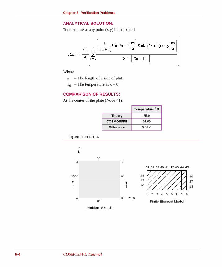
Since the plate and boundary conditions are symmetrical about I-I, only one half of the plate is modeled using SHELL3T elements as shown in the figure.
FFETL01: Steady State Heat Conduction in a Square Plate
(pa
COSMOSFFE Thermal 6-3
Chapter 6 Verification Problems
6-4
ANALYTICAL SOLUTION:
Temperature at any point (x,y) in the plate is
Where
a = The length of a side of plate
T0 = The temperature at x = 0
COMPARISON OF RESULTS:
At the center of the plate (Node 41).
Figure FFETL01–1.
Temperature °C
Theory 25.0
COSMOSFFE 24.99
Difference 0.04%
3938 4037
Y
CD
XA B
I I
0°
0°
0°100°
1 2 3 4 5
41
6
42
7
43
8
44
9
45
28 3619 2710 18
Problem Sketch
Finite Element Model
COSMOSFFE Thermal
Chapter 6 Verification Problems
See ge 6-2.)
TYPE:
Steady-state heat conduction with convection boundary conditions, SHELL4 elements.
REFERENCE:
M. N. Ozisik, “Heat Conduction,” Wiley, New York, 1980.
PROBLEM:
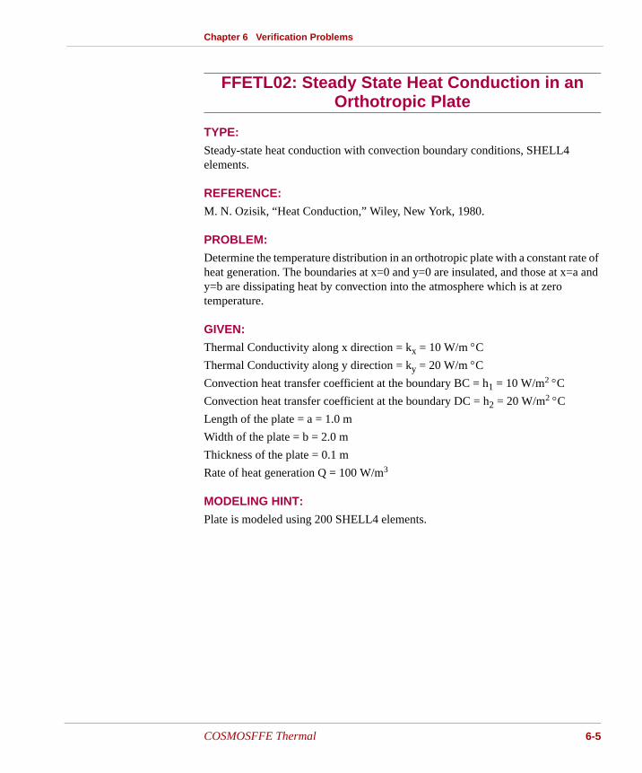
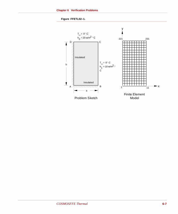
Determine the temperature distribution in an orthotropic plate with a constant rate of heat generation. The boundaries at x=0 and y=0 are insulated, and those at x=a and y=b are dissipating heat by convection into the atmosphere which is at zero temperature.
GIVEN:
Thermal Conductivity along x direction = kx = 10 W/m °C
Thermal Conductivity along y direction = ky = 20 W/m °C
Convection heat transfer coefficient at the boundary BC = h1 = 10 W/m2 °C
Convection heat transfer coefficient at the boundary DC = h2 = 20 W/m2 °C
Length of the plate = a = 1.0 m
Width of the plate = b = 2.0 m
Thickness of the plate = 0.1 m
Rate of heat generation Q = 100 W/m3
MODELING HINT:
Plate is modeled using 200 SHELL4 elements.
FFETL02: Steady State Heat Conduction in an Orthotropic Plate
(pa
COSMOSFFE Thermal 6-5
Chapter 6 Verification Problems
6-6
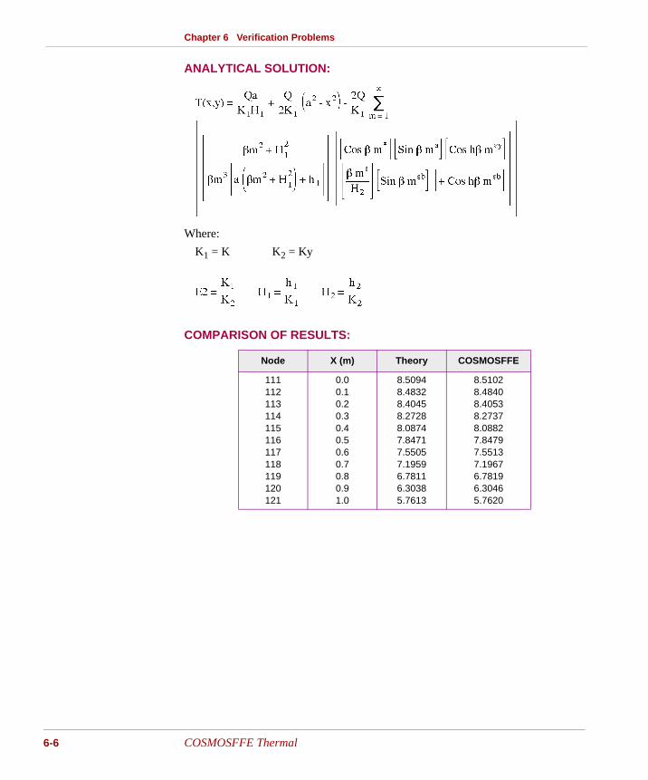
ANALYTICAL SOLUTION:
Where:
K1 = K K2 = Ky
COMPARISON OF RESULTS:
Node X (m) Theory COSMOSFFE
111112113114115116117118119120121
0.00.10.20.30.40.50.60.70.80.91.0
8.50948.48328.40458.27288.08747.84717.55057.19596.78116.30385.7613
8.51028.48408.40538.27378.08827.84797.55137.19676.78196.30465.7620
COSMOSFFE Thermal
Chapter 6 Verification Problems
Figure FFETL02–1.
b
Insulated
Insulated
a
221 231
1 11
y
x
Problem SketchFinite Element
Model
A B
CD
T = 0° C
h = 20 w/m ° C22
∞
T = 0° C
h = 10 w/m °
C
21
∞
COSMOSFFE Thermal 6-7
Chapter 6 Verification Problems
6-8
See ge 6-2.)
TYPE:
Transient heat conduction with convection boundary conditions, PLANE2D elements.
REFERENCE:
J. P. Holman, “Heat Transfer,” McGraw-Hill Book Company, 1976, p. 117.
PROBLEM:
A long aluminum cylinder, 5.0 cm in diameter and initially at 200° C, is suddenly exposed to a convection environment at 70° C and h = 525 W/m2 °C. Calculate the temperature at a radius of 1.25 cm, one minute after the cylinder is exposed to the environment.
GIVEN:
Radius of cylinder = ro = 0.025m
Thermal conductivity = K = 215.0 W/m °C
Mass density = ρ = 2700.0 kg/m3
Specific heat = C = 936.8 J/Kg °C
Initial temperature = T0 = 200° C
Convective heat transfer coefficient = h = 525 w/m2 °C
Ambient temperature = T∞ = 70° C
MODELING HINTS:
Since the cylinder and boundary conditions are axisymmetric, PLANE2D axisymmetric elements are used to model this problem.
FFETL03: Transient Heat Conduction in a Long Cylinder
(pa
COSMOSFFE Thermal
Chapter 6 Verification Problems
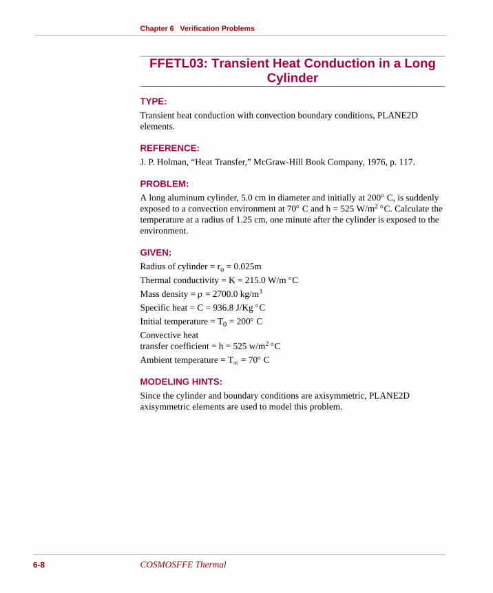
COMPARISON OF RESULTS:
Comparison of solutions is made at r = 0.0125 m (node 21) and at t = 60 sec.
Figure FFETL03–1.
Temperature °C
Theory 118.4
COSMOSFFE 119.49
h, T 8
X
Z
Problem Sketch
r o
Y
2 64 40 42
41391 53
Y
Finite Element Model
X
1 2
r o
COSMOSFFE Thermal 6-9
Chapter 6 Verification Problems
6-10
See ge 6-2.)
TYPE:
Thermal stress analysis, PLANE2D axisymmetric element.
REFERENCE:
Timoshenko and Goodier, “Theory of Elasticity,” McGraw-Hill Book Co., New York, 1961.
PROBLEM:
The hollow cylinder in plane strain is subjected to two independent loading conditions.
1. An internal pressure Pa
2. A steady state axisymmetric temperature distribution due to the following boundary conditions.
At r = 1.0, temperature = 100
At r = 2.0, temperature = 0
GIVEN:
E = 30 x 106 psi
a = 1 in
b = 2 in
ν = 0.3
αx = 1*10-6 / °F
Kx = 1 BTU/in S °F
Pa = 100 psi
Ta = 100° F
Tb = 0° F
✍ The COSMOSM STAR module is required in addition to FFE Thermal, to solve this problem.
FFETL04: Thermal Stresses in a Hollow Cylinder (pa
COSMOSFFE Thermal
Chapter 6 Verification Problems
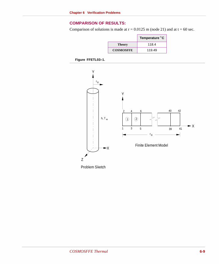
COMPARISON OF RESULTS:
Figure FFETL04–1.
Theory COSMOSFFE
Node 23° F 59.401 59.401
Node 42° F 23.447 23.447
Stresses in Element 7 (Center)
Theory COSMOSM STAR
Tr -398.34 -398.14
Tθ -592.47 -596.38
L
Problem Sketch
Ta
Pa Tr
15
14
28
1 2 3 12
45
x
y
b
31
8
730
C Finite Element Model
16
a
COSMOSFFE Thermal 6-11
Chapter 6 Verification Problems
6-12
See ge 6-2.)
TYPE:
Steady-state heat conduction due to internal heat generation, PLANE2D elements.
REFERENCE:
J. N. Reddy, “An Introduction to the Finite Element Method.” McGraw-Hill Book Co., 1984, p. 260.
PROBLEM:
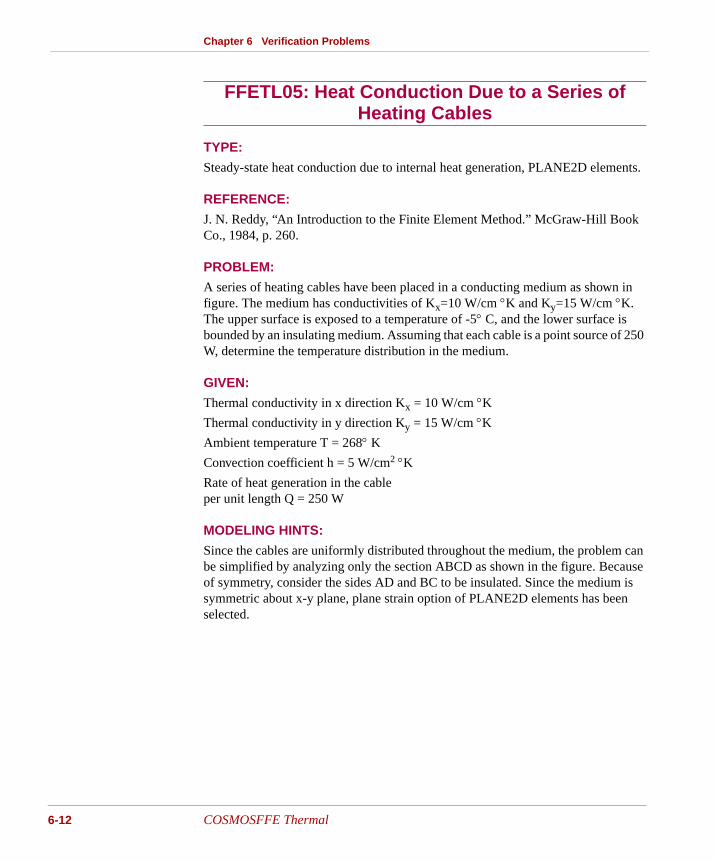
A series of heating cables have been placed in a conducting medium as shown in figure. The medium has conductivities of Kx=10 W/cm °K and Ky=15 W/cm °K. The upper surface is exposed to a temperature of -5° C, and the lower surface is bounded by an insulating medium. Assuming that each cable is a point source of 250 W, determine the temperature distribution in the medium.
GIVEN:
Thermal conductivity in x direction Kx = 10 W/cm °K
Thermal conductivity in y direction Ky = 15 W/cm °K
Ambient temperature T = 268° K
Convection coefficient h = 5 W/cm2 °K
Rate of heat generation in the cable per unit length Q = 250 W
MODELING HINTS:
Since the cables are uniformly distributed throughout the medium, the problem can be simplified by analyzing only the section ABCD as shown in the figure. Because of symmetry, consider the sides AD and BC to be insulated. Since the medium is symmetric about x-y plane, plane strain option of PLANE2D elements has been selected.
FFETL05: Heat Conduction Due to a Series of Heating Cables
(pa
COSMOSFFE Thermal
Chapter 6 Verification Problems
COMPARISON OF RESULTS:
Figure FFETL05–1.
Temperature °C at node 113
Theory ----
COSMOSFFE 299.10
145 153
1 9
D C
113
A B
4
Cables
2
X
4
Y
T = 268 ° K
h = 5 w/cm ° K8
2
Insulated
Finite Element Model
Y
X
Problem Sketch
Cabl
DC
A B
COSMOSFFE Thermal 6-13
Chapter 6 Verification Problems
6-14
See ge 6-2.)
TYPE:
Linear transient heat conduction, TRUSS2D elements.
REFERENCE:
Gupta, C. P., and Prakash, R., “Engineering Heat Transfer,” Nem Chand and Bros., India, 1979, pp. 155-157.
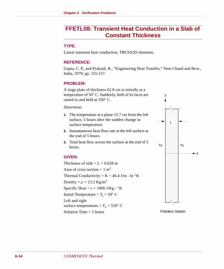
PROBLEM:
A large plate of thickness 62.8 cm is initially at a temperature of 50° C. Suddenly, both of its faces are raised to and held at 550° C.
Determine:
1. The temperature at a plane 15.7 cm from the left surface, 5 hours after the sudden change in surface temperature.
2. Instantaneous heat flow rate at the left surface at the end of 5 hours.
3. Total heat flow across the surface at the end of 5 hours.
GIVEN:
Thickness of slab = L = 0.628 m
Area of cross section = 1 m2
Thermal Conductivity = K = 46.4 J/m - hr °K
Density = ρ = 23.2 Kg/m3
Specific Heat = c = 1000 J/Kg - °K
Initial Temperature = Ti = 50° C
Left and right surface temperatures = Ts = 550° C
Solution Time = 5 hours
FFETL08: Transient Heat Conduction in a Slab of Constant Thickness
(pa
X
L
y
Problem Sketch
Ts Ts
COSMOSFFE Thermal
Chapter 6 Verification Problems
MODELING HINT:
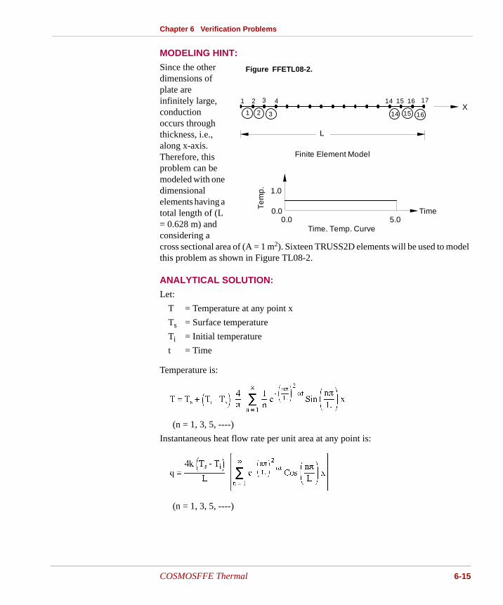
Since the other dimensions of plate are infinitely large, conduction occurs through thickness, i.e., along x-axis. Therefore, this problem can be modeled with one dimensional elements having a total length of (L = 0.628 m) and considering a cross sectional area of (A = 1 m2). Sixteen TRUSS2D elements will be used to model this problem as shown in Figure TL08-2.
ANALYTICAL SOLUTION:
Let:
T = Temperature at any point x
Ts = Surface temperature
Ti = Initial temperature
t = Time
Temperature is:
(n = 1, 3, 5, ----)
Instantaneous heat flow rate per unit area at any point is:
(n = 1, 3, 5, ----)
Figure FFETL08-2.
L
1 2 3 4 17161514
1 2 3 14 15 16X
Finite Element Model
0.05.0
1.0
Time
Te
mp
.
0.0Time. Temp. Curve
COSMOSFFE Thermal 6-15
Chapter 6 Verification Problems
6-16
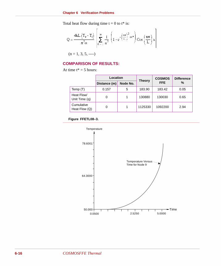
Total heat flow during time t = 0 to t* is:
(n = 1, 3, 5, ----)
COMPARISON OF RESULTS:
At time t* = 5 hours:
Figure FFETL08–3.
LocationTheory
COSMOSFFE
Difference%Distance (m) Node No.
Temp (T) 0.157 5 183.90 183.42 0.05
Heat Flow/ Unit Time (q)
0 1 130880 130030 0.65
Cumulative Heat Flow (Q)
0 1 1125330 1092200 2.94
78.6001
2.52500.0500
Time
64.3000
50.0005.0000
Temperature Versus Time for Node 9
Temperature
COSMOSFFE Thermal
Chapter 6 Verification Problems
See ge 6-2.)
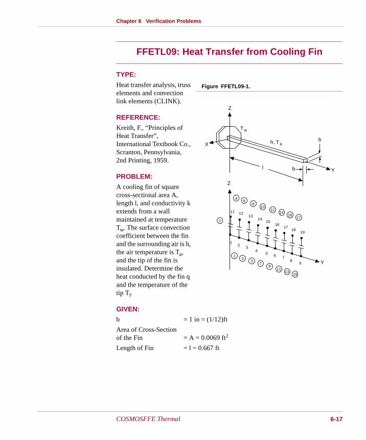
TYPE:
Heat transfer analysis, truss elements and convection link elements (CLINK).
REFERENCE:
Kreith, F., “Principles of Heat Transfer”, International Textbook Co., Scranton, Pennsylvania, 2nd Printing, 1959.
PROBLEM:
A cooling fin of square cross-sectional area A, length l, and conductivity k extends from a wall maintained at temperature Tw. The surface convection coefficient between the fin and the surrounding air is h, the air temperature is Ta, and the tip of the fin is insulated. Determine the heat conducted by the fin q and the temperature of the tip Tl.
GIVEN:
b = 1 in = (1/12)ft
Area of Cross-Section of the Fin = A = 0.0069 ft2
Length of Fin = l = 0.667 ft
FFETL09: Heat Transfer from Cooling Fin (pa
Figure FFETL09-1.
Y
X
Z
13
5 Y
h, T b
T
bl
w
a
Z
1
11 1213
1817
1615
98
7654
32
14
19
79
1113
15
1716
1412
108
64
2
COSMOSFFE Thermal 6-17
Chapter 6 Verification Problems
6-18
Thermal Conductivity = k = 25 BTU/hr-ft- °F
Film Coefficient = h = 1 BTU/hr-ft2- °F
Wall Temperature = Tw = 100° F
Ambient Temperature = Ta = 0° F
CALCULATED INPUT:
The surface convection area per inch length of the fin = 0.02778 ft2.
MODELING HINTS:
The end convection elements are given half the surface area of the interior convection elements. Nodes 11 through 19 are given arbitrary locations.
COMPARISON OF RESULTS:
T at node 9, °F
Theory 68.594
COSMOSFFE 68.615
Difference 0.03%
COSMOSFFE Thermal
Chapter 6 Verification Problems
See ge 6-2.)
TYPE:
Nonlinear heat conduction, TRUSS2D elements.
REFERENCE:
Ozisik, M., “Heat Conduction,” John Wiley and Sons Inc., 1980, pp. 440-443.
PROBLEM:
Determine the temperature distribution in a slab which is insulated on one face, and subjected to a constant temperature on the other face. Assume constant internal heat generation in the slab and a linear variation of thermal conductivity.
GIVEN:
Thickness of the slab = L = 2 m
Internal heat generation = Q = 100,000 W/m3
Thermal conductivity = K = 50 (1 + 2T) W/m ° C
Boundary conditions:
At x = 0, Insulated boundary
At x = L, Prescribed temperature of 100° C
Twenty TRUSS2D elements have been used to model this problem as shown in the figure.
ANALYTICAL SOLUTION:
Steady state heat conduction equation is given by:
Where:
K = K0 (1+ β T), K0 and β are constants.
Q = Rate of internal heat generation.
FFETN01: Heat Conduction with Temperature Dependent Conductivity
(pa
COSMOSFFE Thermal 6-19
Chapter 6 Verification Problems
6-20
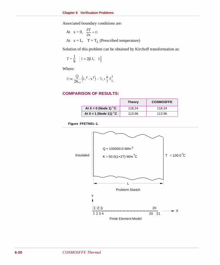
Associated boundary conditions are:
At x = 0,
At x = L, T = TL (Prescribed temperature)
Solution of this problem can be obtained by Kirchoff transformation as:
Where:
COMPARISON OF RESULTS:
Figure FFETN01–1.
Theory COSMOSFFE
At X = 0 (Node 1) °C 118.24 118.24
At X = 1 (Node 11) °C 113.96 113.96
Finite Element Model
Q = 100000.0 W/m
K = 50.0(1+2T) W/m C T = 100.0 Co
Insulated
20
L
Problem Sketch
1 2 3 4 20
1 2 3
21
Y
X
o
3
COSMOSFFE Thermal
Chapter 6 Verification Problems
See ge 6-2.)
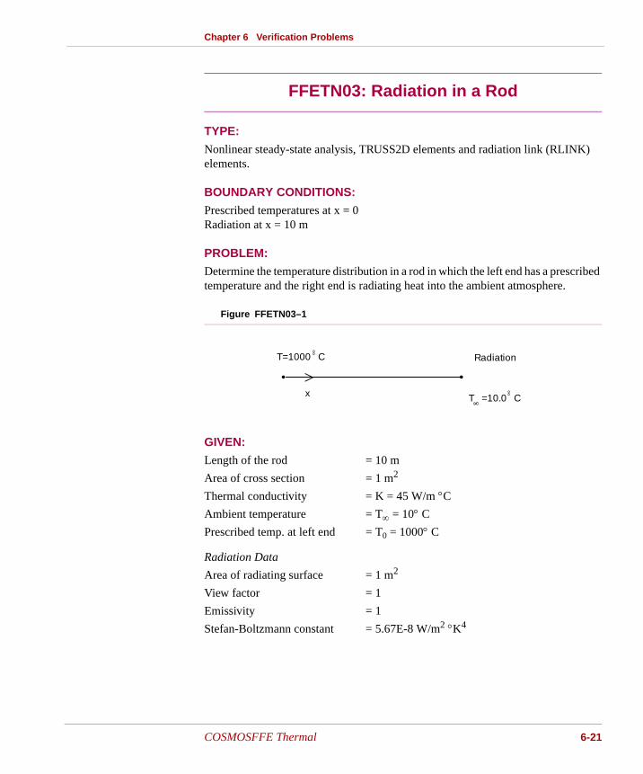
TYPE:
Nonlinear steady-state analysis, TRUSS2D elements and radiation link (RLINK) elements.
BOUNDARY CONDITIONS:
Prescribed temperatures at x = 0Radiation at x = 10 m
PROBLEM:
Determine the temperature distribution in a rod in which the left end has a prescribed temperature and the right end is radiating heat into the ambient atmosphere.
Figure FFETN03–1
GIVEN:
Length of the rod = 10 m
Area of cross section = 1 m2
Thermal conductivity = K = 45 W/m °C
Ambient temperature = T∞ = 10° CPrescribed temp. at left end = T0 = 1000° C
Radiation Data
Area of radiating surface = 1 m2
View factor = 1
Emissivity = 1
Stefan-Boltzmann constant = 5.67E-8 W/m2 °K4
FFETN03: Radiation in a Rod (pa
T=1000 C
T =10.0 C
Radiation
8
x ∞
∞
COSMOSFFE Thermal 6-21
Chapter 6 Verification Problems
6-22
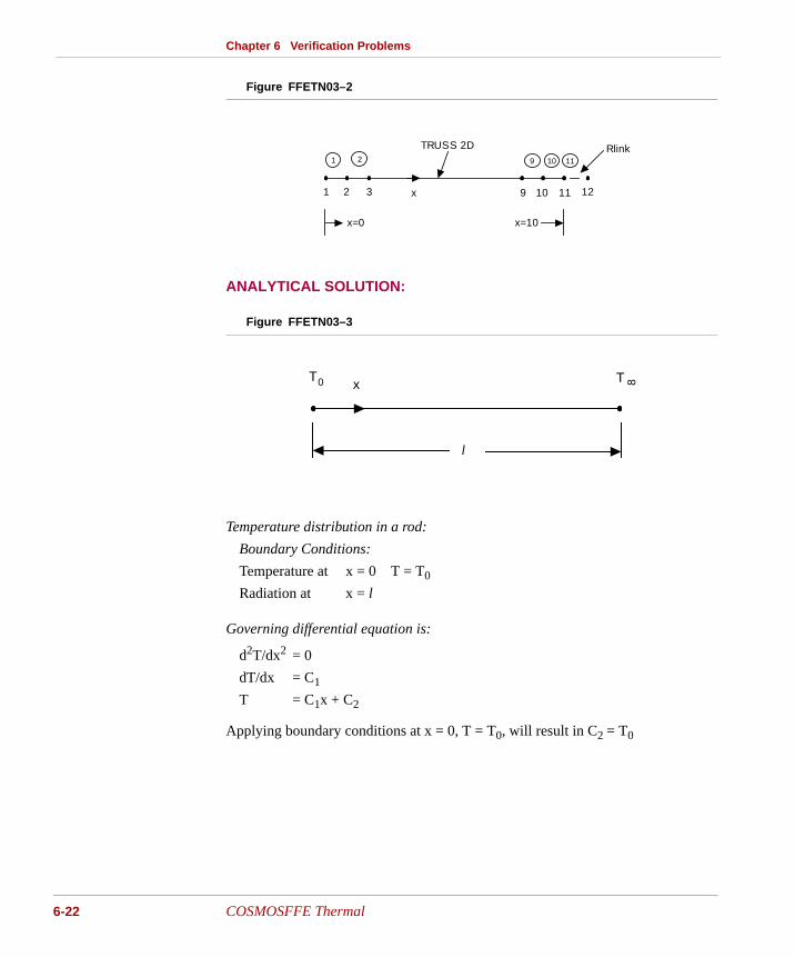
Figure FFETN03–2
ANALYTICAL SOLUTION:
Figure FFETN03–3
Temperature distribution in a rod:
Boundary Conditions:
Temperature at x = 0 T = T0
Radiation at x = l
Governing differential equation is:
d2T/dx2 = 0
dT/dx = C1
T = C1x + C2
Applying boundary conditions at x = 0, T = T0, will result in C2 = T0
TRUSS 2D Rlink
10 11 1291 2 3
1 2 9 10 11
x=0 x=10
x
xT T
l
80
COSMOSFFE Thermal
Chapter 6 Verification Problems
Applying boundary conditions at x = l results in
But we have
Substitute:
σ = 5.67E-8 W/m2 °K4
ε = 1
f = 1
A = 1 m2
K = 45 W/m °K
T0 = 1000° C = 1273.15 °K
T∞ = 10° C = 283.15 °K
COSMOSFFE Thermal 6-23
Chapter 6 Verification Problems
6-24
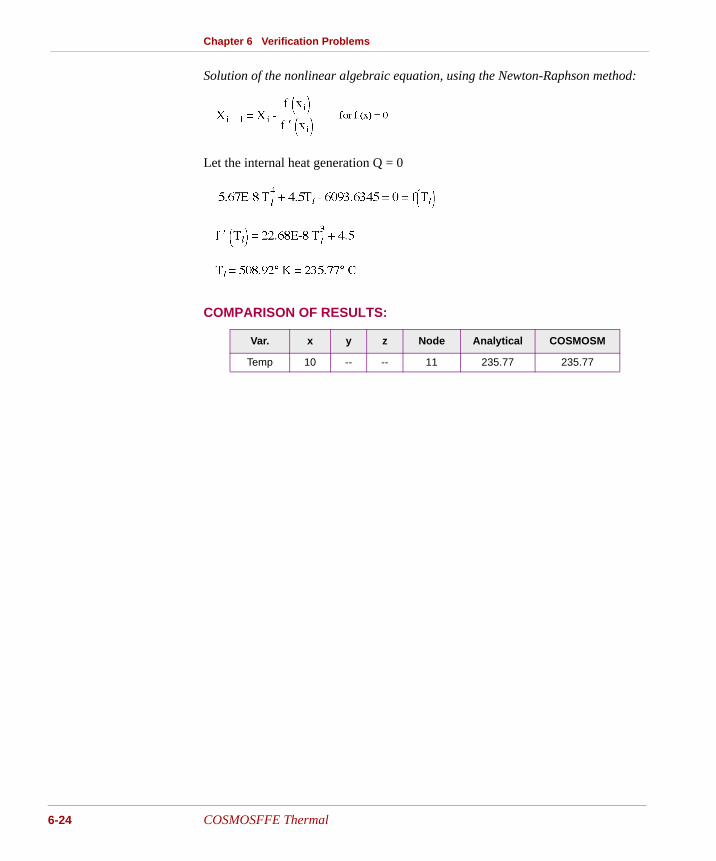
Solution of the nonlinear algebraic equation, using the Newton-Raphson method:
Let the internal heat generation Q = 0
COMPARISON OF RESULTS:
Var. x y z Node Analytical COSMOSM
Temp 10 -- -- 11 235.77 235.77
COSMOSFFE Thermal

A Troubleshooting
Introduction
When you use the COSMOSFFE Thermal module, you may sometimes come across the following error messages, listed alphabetically. Diagnostics and corrective measures for each error messages are provided.
PROBLEM: Bonding is not supported
You have specified bonding of two bodies in your model using the BONDDEF command. Bonding is not supported in this version of FFE Thermal. Delete bonding or use the conventional HSTAR module.
PROBLEM: Cannot restart because previous results are not compatible
Some changes in the model were introduced after the results existing in the database have been calculated. Use the RESTART (Analysis > Restart) com-mand to deactivate the restart option and try again.
PROBLEM: Cannot restart without previous results
You have activated the restart option for transient thermal analysis. Results of the analysis were not found in the database. Use the RESTART (Analysis > Restart) command to deactivate the restart option and try again.
COSMOSFFE Thermal A-1
Appedix A Troubleshooting
A-2
PROBLEM: Cannot restart without results for the starting point
You have activated the restart option for transient thermal analysis. Results of the analysis at the starting solution step were not found in the database.
PROBLEM: Coordinate system <number> is referenced but not defined
Define the missing coordinate system and try again or modify your input such that the named coordinate system is not referred to.
PROBLEM: Degenerate element <number>
Degenerate elements were detected in your model. Degenerate elements are bar elements with 0-length, area elements with 0-area, or solid elements with 0-vol-ume. Use the ECHECK (Meshing > ELEMENTS > Check Element) command to correct the problem and automatically delete bar elements whose length is less than PTTOL, area elements whose area is less than PTTOL square, and solid elements whose volume is less than PTTOL cubed. The point tolerance is defined by the PTTOL (Geometry > POINTS > Merge Tolerance) command.
PROBLEM: Element <number> has unsupported type
The given element is associated with an element group that is not supported in this release of FFE Thermal. Use the conventional solver, or redefine the ele-ment group if possible.
PROBLEM: Element <number> is pyramid shaped, which is not supported
The named element belongs to a SOLID element group. The nodes defining a face of the solid have collapsed to a single point. This type of collapsed element is not currently supported by COSMOSFFE Thermal. This element may have been defined manually or resulted from the parametric meshing of a volume with a very sharp edges or corners. Delete the mesh, define a TETRA4, or TETRA10 element group, and use automatic meshing instead of parametric meshing. Prism-shaped elements are automatically supported.
PROBLEM: Error while closing a temporary file
An I/O error occurred while closing a temporary file.
COSMOSFFE Thermal
Chapter A Troubleshooting
PROBLEM: Error while positioning a temporary file
An I/O error has occurred while reading information from a temporary working file.
PROBLEM: Error while reading file <filename>
An I/O error has occurred while reading from the named file which is part of the COSMOSM database. The file may have been corrupted. Check the integrity of your hard disk, reconstruct the model by creating a new problem and using the FILE (File > Load...) command, and try again.
PROBLEM: Error while reading from a temporary file
An I/O error has occurred while reading information from a temporary working file.
PROBLEM: Error while writing to a temporary file
An error occurred while writing data to the temporary file. Check the available disk space, and the integrity of your system, especially the hard disk. Recon-struct the database and try again.
PROBLEM: Error while writing to file <filename>
An error occurred while writing data to the named file. Check the integrity of your system, especially the hard disk. Reconstruct the database and try again.
PROBLEM: File <filename> does not contain necessary data
The named file does not contain the expected data in the expected format. Either the file is corrupted, overwritten, or created by a different COSMOSM version.
PROBLEM: File <filename> has invalid format
The format of the data in the named file is not as expected. Either the file is cor-rupted, overwritten, or created by a different COSMOSM version.
PROBLEM: Improper axisymmetric model
The defined axisymmetric model is improper. Axisymmetric elements must be defined in the global X-Y plane with the Y-axis as the axis of symmetry.
COSMOSFFE Thermal A-3
Appedix A Troubleshooting
A-4
PROBLEM: Improper mesh near element <number>
The mesh elements are not compatible in the neighborhood of the named ele-ment. This can be the result of improper node merging, invalid parametric tetra-hedral mesh, or invalid manually created elements.
PROBLEM: Improper mesh, properties, or boundary conditions
Either the mesh, material properties, or boundary conditions of the model have been improperly defined. Use the R_CHECK (Analysis > Run Check) com-mand to check the elements. Also list and examine the material properties and boundary conditions.
PROBLEM: Incompatible element groups
The generated mesh connects elements with incompatible element groups to each other. Try to use other alternatives such that connected elements have com-patible degrees of freedom.
PROBLEM: Internal error # <number>
An internal error has occurred. Record the error number and report to SRAC.
PROBLEM: Invalid combination of first and second order elements
First order (linear) and second order (parabolic) elements are connected to each other resulting in incompatible common edges. An example is connecting TETRA4 elements to TETRA10 elements. Use the ECHANGE (Meshing > Element Order) command to fix the problem by raising the order of first order elements or lowering the order of second order elements. It is recommended, though not necessary to change the element group(s).
PROBLEM: Invalid curve
An invalid temperature or time curve has been found. Verify your input. The ACTXYPRE (Display XY PLOTS > Activate Pre-Proc) and XYPLOT (Display XY PLOTS > Plot Curves) commands may be used to plot time and tempera-ture curves. Redefine the invalid curves using the CURDEF (LoadsBC > FUNC-TION CURVE > Time/Temp Curve) command and try again. A corruption in the database is possible.
COSMOSFFE Thermal
Chapter A Troubleshooting
PROBLEM: Invalid order of nodes for element <number>
The number of nodes used to define the specified element is invalid. Use the (Edit > LIST > Element Groups) and ELIST (Edit > LIST > Elements) com-mands to find the error. The R_CHECK (Analysis > Run Check) command will also detect such errors.
PROBLEM: Invalid time interval for the analysis <start>, <end>
The time interval specified for the transient thermal analysis is invalid. Use the TIMES (LoadsBC > LOAD OPTIONS > Time Parameter) command to correct the error.
PROBLEM: Maximum number of nonlinear iterations <number> exceeded
The maximum allowable number of nonlinear iterations has been exceeded without conversion. Check your input. Allow a higher number of iterations if no errors are found. Use a smaller time interval for transient analysis.
PROBLEM: Not enough boundary conditions
None or inadequate boundary conditions specified. Use commands in the LoadsBC > HEAT TRANSFER menu to check your input. Specify more bound-ary conditions and try again.
PROBLEM: Out of memory or swap space
Available virtual memory is not sufficient to run this problem.
On UNIX systems contact your system administrator to increase size of the swap space.
PROBLEM: Too many time steps
The number of time steps for transient thermal analysis exceeded the maximum allowed number which is currently 2400.
PROBLEM: Unable to create a temporary file
The program could not create a temporary file. Check the integrity of your sys-tem and verify that adequate disk space is available.
COSMOSFFE Thermal A-5
Appedix A Troubleshooting
A-6
PROBLEM: Unable to create file <filename>
The program could not create the named file. Check the integrity of your system and verify that adequate disk space is available.
PROBLEM: Unable to open file <filename>
The program could not open the named file which is part of the COSMOSM database. The file may have been deleted. Check the integrity of your hard disk, reconstruct the model by creating a new problem and using the FILE (File > Load...) command.
PROBLEM: Unable to open problem database
The program could not open the database for this problem. Verify that the data-base files for this problem exist in the proper path and directory specified and that the correct version is being used. Also check the integrity of your system and verify that adequate disk space is available.
PROBLEM: Unexpected end of file while reading <filename>
An end-file mark was found before reading all needed data from the named file. Check related input, fix the problem if any, and try again. Regenerate the file if possible, check the integrity of your system and reconstruct the database through the FILE (File > Load...) command if the problem could not be fixed otherwise.
PROBLEM: You are not authorized to use this type of analysis
You are not authorized to use this type of analysis. Use the PRODUCT_INFO (Control > MISCELLANEOUS > Product Info) command to get a list of the modules you are authorized to use. Contact S.R.A.C.
PROBLEM: Zero or negative cross section area for element <number>
The cross sectional area of the specified element is zero or negative. Use the ELIST (Edit > LIST > Elements) command to find the associated real constant set and then use the RCLIST (Edit > LIST > Real Constants) command to list the cross sectional area. Use the RCONST (Propsets > Real Constant) com-mand to specify a positive value.
COSMOSFFE Thermal
Chapter A Troubleshooting
PROBLEM: Zero or negative heat conductivity for element <number>
The heat conductivity specified for this element is zero or negative. Use the ELIST (Edit > LIST > Elements) command to find the associated material prop-erty set and then use the MPLIST (Edit > LIST > Material Props) command to list the material properties in the associated set. Use the MPROP (Propsets > Material Property) command to specify a positive value.
PROBLEM: Zero or negative real constant for radiation link element <number>
An invalid value has been specified in the real constant associated with the spec-ified element. Use the ELIST (Edit > LIST > Elements) command to find the associated real constant set and then use the RCLIST (Edit > LIST > Real Con-stants) command to list the set and check your input for the radiating surface area, the view factor, emissivity, and the Stefan-Boltzman constant. Use the RCONST (Propsets > Real Constant) command to fix the error.
PROBLEM: Zero or negative thickness for element <number>
The thickness of the specified element is zero or negative. Use the ELIST (Edit > LIST > Elements) command to find the associated real constant set and then use the RCLIST (Edit > LIST > Real Constants) command to list the thickness. Use the RCONST (Propsets > Real Constant) command to specify a positive value.
PROBLEM: Zero or negative time increment
The time increment specified by the TIMES command is invalid. Use the TIMES (LoadsBC > LOAD OPTIONS > Time Parameter) command to specify a posi-tive value.
COSMOSFFE Thermal A-7

A-8
COSMOSFFE Thermal
Index
AActivate Post-Proc 4-6
Bbeam element 3-1BEAM2D 3-1BEAM3D 3-1boundary condition 1-1
Cchange element A-4Change El-Prop 3-2check element A-2CLINK 3-1, 6-2convection 1-2, 5-18, 6-5, 6-8convergence tolerance 4-6
DData Check 4-7Default Meshing 5-11delete mesh 5-7delete polyhedron 5-9
EElement Group 3-2element library 3-1error messages A-1
Extrusion 5-4, 5-11
FFFE Static Options 4-5FFE Thermal Options 4-5, 5-1first order 4-6
Hheat flux 1-2
Llinear 5-1list element groups A-5
Mmass matrix 4-6material properties A-4, A-7
NNew Property Set 3-2nonlinear 5-1, 5-10
OOffset Temperature 5-13
PPLANE2D 6-2Plot Curves 4-6
postprocessing 4-2preprocessing 4-2Product Info A-6Property Set 3-2
Rradiation 1-3Read Temp as Load 4-5RLINK 3-1, 6-2Run Check A-5Run Static Analysis 4-5Run Thermal Analysis 4-6
Ssecond order 4-6Set Entity 4-4SHELL3 3-1SHELL3T 3-1, 6-2SHELL4 3-1, 6-2SHELL4T 3-1size limitations 2-3SOLID 3-1steady-state 4-5Stefan-Boltzmann Constant 5-13surfaces 5-3
COSMOSFFE Thermal I-1
Index
Ttemperature 1-2TETRA10 3-2TETRA4 3-2Thermal Analysis Options 4-5thermal stress 4-5Time/Temp Curve 4-4, A-4transient 4-5, 4-6TRIANG 3-2TRUSS 6-2TRUSS2D 3-2, 6-2TRUSS3D 3-2
Uunits 1-3
I-2 COSMOSFFE Thermal