Embed Size (px)
Citation preview
UNIVERSITE DE GENEVE FACULTE DES SCIENCESDepartement de physique theorique Professeur R. DURRER
Cosmology of Brane Universes
and Brane Gases
THESE
presentee a la Faculte des sciences de l’Universite de Geneve
pour l’obtention du grade de
Docteur es sciences, mention physique
par
Timon Georg BOEHMde
Bale (BS)
These N 3481
GENEVE
Atelier de reproduction de la Section de physique
2004

.
Abstract
The standard big bang model gives a fairly good description of the cosmologicalevolution of our universe from shortly after the big bang to the present. Theexistence of an initial singularity, however, might be viewed as unsatisfactory in acomprehensive model of the universe. Moreover, if this singularity indeed exists,we are lacking initial conditions which tell us in what state the universe emergedfrom the big bang.
The advent of string theory as a promising candidate for a theory of quantumgravity opened up new possibilities to understand our universe. The hope is thatstring theory can resolve the initial singularity problem and, in addition, provideinitial conditions.
String theory makes a number of predictions such as extra-dimensions, theexistence of p-branes (fundamental objects with p spatial dimensions) as wellas several new particles. Consequently, over the past few years, a new field ofresearch emerged, which investigates how these predictions manifest themselvesin a cosmological context. In particular, the idea that our universe is a 3-braneembedded in a higher-dimensional space received a lot of attention.
In this thesis we investigate the dynamical and perturbative behavior of stringtheory inspired cosmological models. After an introduction to extra-dimensionsand p-branes, we identify our universe with a 3-brane embedded in a 5-dimensionalbulk space-time. We then study the cosmology and the evolution of perturbationsdue to the motion of this brane through the higher-dimensional space-time. Se-condly, we point out the dynamical instabilities of the Randall-Sundrum model.And thirdly, vector perturbations on the brane induced by perturbations in thebulk are calculated, and the resulting CMB power spectrum is estimated. Inall cases, dynamical instabilities are encountered, which suggests that existingattempts to realize cosmology on branes are at least questionable.
In the last part of this thesis, we study string and brane gas cosmology. In thisscenario, the role of strings and branes is to drive the background dynamics. Astring theory specific symmetry between large and small scales (T-duality) is usedto avoid the initial big bang singularity. We show that the evolution of an initiallysmall and compact nine-dimensional space-time leads to three large dimensions,which then become our visible universe. Brane gas cosmology seems to us verypromising to bring together string theory and cosmology.
This work is only part of a tremendously growing flood of literature, but wehope that it is nevertheless a piece of mosaic in the work of art which is science.We hope that the interplay between string theory and cosmology enables us toadvance to new spheres and dimensions (see Fig. 1).
i

.
ii
Figure 1:
iii

.
iv
Remerciements
Je tiens d’abord a remercier ma directrice de these, Ruth Durrer, pour m’avoirenseigne les sujets fascinants de la relativite generale et cosmologie, mais egalementpour son soutien et ses conseils, ainsi que sa comprehension et sa patience.
J’ai eu le plaisir de collaborer avec Robert Brandenberger, Carsten van deBruck, Christophe Ringeval et Daniele Steer.
Je remercie les membres du groupe de cosmologie de l’Universite de Geneve:Cyril Cartier, Stefano Foffa, Yasmin Friedmann, Kerstin Kunze, Simone Lelli,Michele Maggiore, Alain Riazuelo, Anna Rissone, Marti Ruiz-Altaba, MarcusRuser, Riccardo Sturani, Filippo Vernizzi, Peter Wittwer et en particulier Christo-phe Ringeval et Roberto Trotta ainsi que les cosmologistes musicaux ThierryBaertschiger et Sam Leach.
Pendant cette these j’ai eu la chance de passer un mois au Laboratoire dephysique theorique a Paris-Orsay, ou j’ai profite de nombreuses discussions avecEmilien Dudas et Jihad Mourad.
Et finalement je suis reconnaissant aux mains magiques de Cyril Cartier et An-dreas Malaspinas pour leur soutien ‘informatique et latex’ ainsi qu’a Sam Leachet a Christophe Ringeval pour avoir corrige les parties anglaises et francaises decette these.
Examinateurs
Le jury de cette these se compose de
• Prof. Pierre Binetruy, Universite Paris-XI, Orsay Cedex, France.
• Prof. Robert Brandenberger, Brown University, Providence, USA.
• Prof. Ruth Durrer, Universite de Geneve, Suisse.
• Prof. Michele Maggiore, Universite de Geneve, Suisse.
Je tiens a les remercier d’avoir accepte de faire partie du jury de ma these.
v

.
vi

Meinen Eltern gewidmet
vii

.
viii
Contents
Abstract i
Remerciements v
Resume 1
Introduction 13
I EXTRA-DIMENSIONS AND BRANES 19
1 The cosmological standard model 211.1 Isotropy and homogeneity of the observable universe . . . . . . . . 221.2 Friedmann-Lemaıtre space-times . . . . . . . . . . . . . . . . . . . 23
1.2.1 Isotropic manifolds . . . . . . . . . . . . . . . . . . . . . . . 231.2.2 Riemannian spaces of constant curvature . . . . . . . . . . 241.2.3 The metric of Friedmann-Lemaıtre space-times . . . . . . . 25
1.3 The gravitational field equations . . . . . . . . . . . . . . . . . . . 251.3.1 Cosmological equations . . . . . . . . . . . . . . . . . . . . 261.3.2 Energy ‘conservation’ . . . . . . . . . . . . . . . . . . . . . 271.3.3 Past and future of a Friedmann-Lemaıtre universe . . . . . 271.3.4 Cosmological solutions . . . . . . . . . . . . . . . . . . . . . 291.3.5 A remark on conformal time . . . . . . . . . . . . . . . . . 30
1.4 The cosmic microwave background . . . . . . . . . . . . . . . . . . 311.5 Appendix . . . . . . . . . . . . . . . . . . . . . . . . . . . . . . . . 32
2 Extra-dimensions 352.1 Motivation . . . . . . . . . . . . . . . . . . . . . . . . . . . . . . . 362.2 Supergravity . . . . . . . . . . . . . . . . . . . . . . . . . . . . . . 372.3 String theory . . . . . . . . . . . . . . . . . . . . . . . . . . . . . . 39
2.3.1 Introductory remarks . . . . . . . . . . . . . . . . . . . . . 392.3.2 10- and 26-dimensional space-times . . . . . . . . . . . . . . 412.3.3 Mass spectrum of a closed string on a compact direction . . 44
2.4 Geometrical remarks on compact spaces . . . . . . . . . . . . . . . 46
ix
2.4.1 Spaces with positive, negative, and zero Ricci curvature . . 47
2.4.2 The gravitational field equations . . . . . . . . . . . . . . . 48
2.5 Toroidal compactification . . . . . . . . . . . . . . . . . . . . . . . 50
2.5.1 Kaluza-Klein states . . . . . . . . . . . . . . . . . . . . . . 50
2.5.2 Dimensional reduction of the action . . . . . . . . . . . . . 52
2.5.3 Horava-Witten compactification . . . . . . . . . . . . . . . 53
2.6 The modifications of Newton’s law . . . . . . . . . . . . . . . . . . 54
2.6.1 Newton’s law in d non compact spatial dimensions . . . . . 54
2.6.2 Newton’s law with n compact extra-dimensions . . . . . . . 55
2.7 The hierarchy problem . . . . . . . . . . . . . . . . . . . . . . . . . 57
2.7.1 Fundamental and effective Planck mass . . . . . . . . . . . 57
2.7.2 The idea of ‘large’ extra-dimensions . . . . . . . . . . . . . 58
3 Branes 61
3.1 Extended objects . . . . . . . . . . . . . . . . . . . . . . . . . . . . 62
3.2 Differential geometrical preliminaries . . . . . . . . . . . . . . . . . 62
3.2.1 Embedding of branes . . . . . . . . . . . . . . . . . . . . . . 63
3.2.2 The first fundamental form . . . . . . . . . . . . . . . . . . 64
3.2.3 The second fundamental form . . . . . . . . . . . . . . . . . 65
3.2.4 First and second fundamental form for one co-dimension . . 66
3.2.5 The equations of Gauss, Codazzi and Mainardi . . . . . . . 68
3.2.6 Junction conditions . . . . . . . . . . . . . . . . . . . . . . 70
3.3 Branes from supergravity . . . . . . . . . . . . . . . . . . . . . . . 72
3.3.1 The black p-brane geometry . . . . . . . . . . . . . . . . . . 72
3.3.2 Anti-de Sitter space-time . . . . . . . . . . . . . . . . . . . 74
3.4 Branes from string theory . . . . . . . . . . . . . . . . . . . . . . . 76
3.4.1 T-duality for open strings . . . . . . . . . . . . . . . . . . . 76
3.4.2 Some properties of D-branes . . . . . . . . . . . . . . . . . 77
II BRANE COSMOLOGY 81
4 Cosmology on a probe brane 83
4.1 Introduction . . . . . . . . . . . . . . . . . . . . . . . . . . . . . . . 84
4.2 Probe brane dynamics . . . . . . . . . . . . . . . . . . . . . . . . . 84
4.3 Friedmann equation . . . . . . . . . . . . . . . . . . . . . . . . . . 86
4.4 Discussion . . . . . . . . . . . . . . . . . . . . . . . . . . . . . . . . 88
5 Perturbations on a moving D3-brane and mirage cosmology (ar-ticle) 89
5.1 Introduction . . . . . . . . . . . . . . . . . . . . . . . . . . . . . . . 91
5.2 Unperturbed dynamics of the D3-brane . . . . . . . . . . . . . . . 94
5.2.1 Background metric and brane scale factor . . . . . . . . . . 94
5.2.2 Brane action and bulk 4-form field . . . . . . . . . . . . . . 95
x
5.2.3 Brane dynamics and Friedmann equation . . . . . . . . . . 99
5.3 Perturbed equations of motion . . . . . . . . . . . . . . . . . . . . 101
5.3.1 The second order action . . . . . . . . . . . . . . . . . . . . 101
5.3.2 Evolution of perturbations in brane time τ . . . . . . . . . 104
5.3.3 Comments on an analysis in conformal time η . . . . . . . . 110
5.4 Bardeen potentials . . . . . . . . . . . . . . . . . . . . . . . . . . . 112
5.5 Conclusions . . . . . . . . . . . . . . . . . . . . . . . . . . . . . . . 115
6 Cosmology on a back-reacting brane 117
6.1 Introduction . . . . . . . . . . . . . . . . . . . . . . . . . . . . . . . 118
6.2 The Randall-Sundrum model . . . . . . . . . . . . . . . . . . . . . 119
6.2.1 Warped geometry solution . . . . . . . . . . . . . . . . . . . 119
6.2.2 Scales and the hierarchy problem . . . . . . . . . . . . . . . 120
6.2.3 Non compact extra-dimension . . . . . . . . . . . . . . . . . 121
6.3 Brane cosmological equations . . . . . . . . . . . . . . . . . . . . . 122
6.3.1 The five-dimensional Einstein equations . . . . . . . . . . . 122
6.3.2 Junction conditions and the Friedmann equation of branecosmology . . . . . . . . . . . . . . . . . . . . . . . . . . . . 124
6.3.3 Solution of the Friedmann equation and recovering standardcosmology . . . . . . . . . . . . . . . . . . . . . . . . . . . . 125
6.4 Einstein’s equations on the brane world . . . . . . . . . . . . . . . 127
7 Dynamical instabilities of the Randall-Sundrum model (article)131
7.1 Introduction . . . . . . . . . . . . . . . . . . . . . . . . . . . . . . . 133
7.2 Equations of motion . . . . . . . . . . . . . . . . . . . . . . . . . . 135
7.2.1 General case . . . . . . . . . . . . . . . . . . . . . . . . . . 135
7.2.2 Special case: The Randall–Sundrum model . . . . . . . . . 138
7.3 A dynamical brane . . . . . . . . . . . . . . . . . . . . . . . . . . . 139
7.4 Gauge Invariant Perturbation equations . . . . . . . . . . . . . . . 144
7.4.1 Perturbations of the Randall–Sundrum model . . . . . . . . 144
7.4.2 Gauge invariant perturbation equations . . . . . . . . . . . 145
7.5 Results and Conclusions . . . . . . . . . . . . . . . . . . . . . . . . 148
8 On CMB anisotropies in a brane universe 151
8.1 Introduction . . . . . . . . . . . . . . . . . . . . . . . . . . . . . . . 152
8.2 Bulk vector perturbations in 4 + 1 dimensions . . . . . . . . . . . . 153
8.2.1 Background variables . . . . . . . . . . . . . . . . . . . . . 153
8.2.2 Perturbed metric and gauge invariant variables . . . . . . . 153
8.2.3 Perturbed Einstein equations . . . . . . . . . . . . . . . . . 155
8.3 Temperature fluctuations in the CMB . . . . . . . . . . . . . . . . 157
8.3.1 Induced vector perturbations on the brane . . . . . . . . . . 157
8.3.2 Sources of CMB anisotropies . . . . . . . . . . . . . . . . . 158
8.3.3 Temperature fluctuations as a function of the perturbationvariables . . . . . . . . . . . . . . . . . . . . . . . . . . . . . 159
xi
8.3.4 The perturbed geodesic equation . . . . . . . . . . . . . . . 1618.4 Observation of the temperature fluctuations . . . . . . . . . . . . . 1638.5 The C`’s of vector perturbations . . . . . . . . . . . . . . . . . . . 165
9 CMB anisotropies from vector perturbations in the bulk (article)1699.1 Introduction . . . . . . . . . . . . . . . . . . . . . . . . . . . . . . . 1719.2 Background . . . . . . . . . . . . . . . . . . . . . . . . . . . . . . . 173
9.2.1 Embedding and motion of the brane . . . . . . . . . . . . . 1739.2.2 Extrinsic curvature and unperturbed junction conditions . . 175
9.3 Gauge invariant perturbation equations in the bulk . . . . . . . . . 1789.3.1 Bulk perturbation variables . . . . . . . . . . . . . . . . . . 1789.3.2 Bulk perturbation equations and solutions . . . . . . . . . . 179
9.4 The induced perturbations on the brane . . . . . . . . . . . . . . . 1839.4.1 Brane perturbation variables . . . . . . . . . . . . . . . . . 1839.4.2 Perturbed induced metric and extrinsic curvature . . . . . . 1849.4.3 Perturbed junction conditions and solutions . . . . . . . . . 185
9.5 CMB anisotropies . . . . . . . . . . . . . . . . . . . . . . . . . . . . 1869.6 Conclusion . . . . . . . . . . . . . . . . . . . . . . . . . . . . . . . 1919.7 Appendix . . . . . . . . . . . . . . . . . . . . . . . . . . . . . . . . 193
9.7.1 Comparison with the Randall-Sundrum model . . . . . . . 1939.7.2 CMB angular power spectrum . . . . . . . . . . . . . . . . 195
III BRANE GAS COSMOLOGY 203
10 The cosmology of string gases 20510.1 Avoiding the initial singularity . . . . . . . . . . . . . . . . . . . . 206
10.1.1 T-duality . . . . . . . . . . . . . . . . . . . . . . . . . . . . 20610.1.2 String thermodynamics . . . . . . . . . . . . . . . . . . . . 207
10.2 Why is space three-dimensional? . . . . . . . . . . . . . . . . . . . 20910.3 Equation of state of a brane gas . . . . . . . . . . . . . . . . . . . . 212
11 On T-duality in brane gas cosmology (article) 21711.1 Introduction . . . . . . . . . . . . . . . . . . . . . . . . . . . . . . . 21911.2 Review of brane gas cosmology . . . . . . . . . . . . . . . . . . . . 22111.3 Energy, momentum, and pressure of p-branes . . . . . . . . . . . . 22311.4 Winding states and T-duality . . . . . . . . . . . . . . . . . . . . . 22611.5 Mass spectra and T-duality . . . . . . . . . . . . . . . . . . . . . . 227
11.5.1 Masses of p-branes with single winding . . . . . . . . . . . . 22711.5.2 Multiple windings . . . . . . . . . . . . . . . . . . . . . . . 229
11.6 Cosmological implications and discussion . . . . . . . . . . . . . . . 23011.7 Appendix . . . . . . . . . . . . . . . . . . . . . . . . . . . . . . . . 231
Conclusions 233
xii

Resume
2 RESUME
Introduction
La theorie des cordes est une theorie fondamentale, qui unifie la gravitationet les interactions de jauge d’une maniere consistante et renormalisable. Etantune theorie de la gravite quantique, on pense, qu’elle a joue un role important totdans l’histoire de l’univers, et qu’elle est necessaire a la comprehension de celui-ci.D’autre part, due a la recolte d’une grande quantite de donnees astrophysiques,la cosmologie est devenue une science de precision. On espere pouvoir testerpour la premiere fois les predictions de la theorie des cordes dans les processuscosmologiques.
Pendant les annees passees l’interaction entre la theorie des cordes et la cos-mologie est devenue un domaine de recherche important, qui a apporte de nou-velles connaissances aux deux sujets. L’objectif de cette these est d’etudier, com-ment se manifestent certaines predictions de la theorie des cordes dans un cadrecosmologique. Cette these comporte quatre articles, qui ont ete elabores en col-laboration avec d’autres chercheurs, ainsi que des chaptires d’introduction et derevue.
Le modele standard de la cosmologie
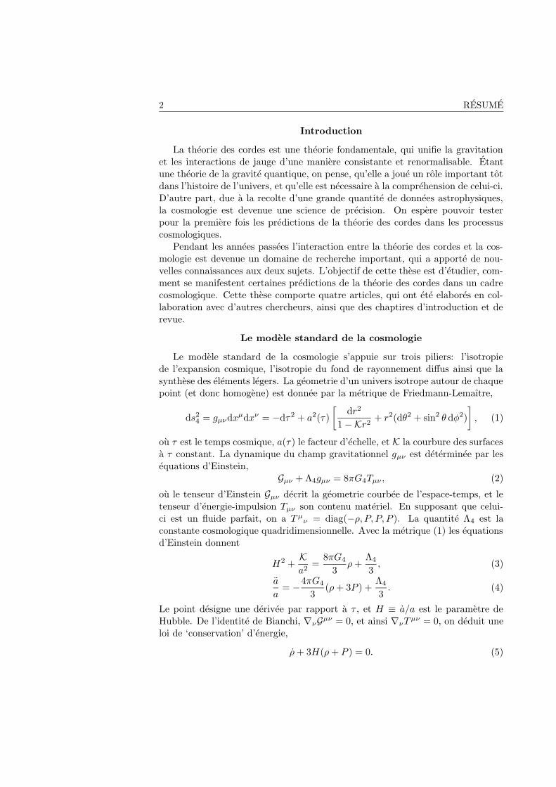
Le modele standard de la cosmologie s’appuie sur trois piliers: l’isotropiede l’expansion cosmique, l’isotropie du fond de rayonnement diffus ainsi que lasynthese des elements legers. La geometrie d’un univers isotrope autour de chaquepoint (et donc homogene) est donnee par la metrique de Friedmann-Lemaıtre,
ds24 = gµνdxµdxν = −dτ2 + a2(τ)
[dr2
1−Kr2 + r2(dθ2 + sin2 θ dφ2)
], (1)
ou τ est le temps cosmique, a(τ) le facteur d’echelle, et K la courbure des surfacesa τ constant. La dynamique du champ gravitationnel gµν est determinee par lesequations d’Einstein,
Gµν + Λ4gµν = 8πG4Tµν , (2)
ou le tenseur d’Einstein Gµν decrit la geometrie courbee de l’espace-temps, et letenseur d’energie-impulsion Tµν son contenu materiel. En supposant que celui-ci est un fluide parfait, on a T µ
ν = diag(−ρ, P, P, P ). La quantite Λ4 est laconstante cosmologique quadridimensionnelle. Avec la metrique (1) les equationsd’Einstein donnent
H2 +Ka2
=8πG4
3ρ+
Λ4
3, (3)
a
a= −4πG4
3(ρ+ 3P ) +
Λ4
3. (4)
Le point designe une derivee par rapport a τ , et H ≡ a/a est le parametre deHubble. De l’identite de Bianchi, ∇νGµν = 0, et ainsi ∇νT
µν = 0, on deduit uneloi de ‘conservation’ d’energie,
ρ+ 3H(ρ+ P ) = 0. (5)
3
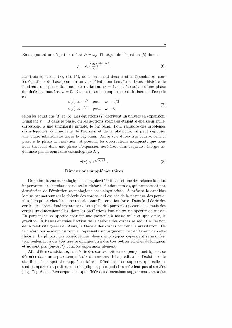
En supposant une equation d’etat P = ωρ, l’integral de l’equation (5) donne
ρ = ρi
(ai
a
)3(1+ω)
. (6)
Les trois equations (3), (4), (5), dont seulement deux sont independantes, sontles equations de base pour un univers Friedmann-Lemaıtre. Dans l’histoire del’univers, une phase dominee par radiation, ω = 1/3, a ete suivie d’une phasedominee par matiere, ω = 0. Dans ces cas le comportement du facteur d’echelleest
a(τ) ∝ τ1/2 pour ω = 1/3,
a(τ) ∝ τ2/3 pour ω = 0,(7)
selon les equations (3) et (6). Les equations (7) decrivent un univers en expansion.L’instant τ = 0 dans le passe, ou les sections spatiales etaient d’epaisseur nulle,correspond a une singularite initiale, le big bang. Pour resoudre des problemescosmologiques, comme celui de l’horizon et de la platitude, on peut supposerune phase inflationaire apres le big bang. Apres une duree tres courte, celle-cipasse a la phase de radiation. A present, les observations indiquent, que nousnous trouvons dans une phase d’expansion acceleree, dans laquelle l’energie estdominee par la constante cosmologique Λ4,
a(τ) ∝ e√
Λ4/3τ . (8)
Dimensions supplementaires
Du point de vue cosmologique, la singularite initiale est une des raisons les plusimportantes de chercher des nouvelles theories fondamentales, qui permettent unedescription de l’evolution cosmologique sans singularites. A present le candidatle plus prometteur est la theorie des cordes, qui est nee de la physique des partic-ules, lorsqu’ on cherchait une theorie pour l’interaction forte. Dans la theorie descordes, les objets fondamentaux ne sont plus des particules ponctuelles, mais descordes unidimensionnelles, dont les oscillations font naıtre un spectre de masse.En particulier, ce spectre contient une particule a masse nulle et spin deux, legraviton. A basses energies l’action de la theorie des cordes se reduit a l’actionde la relativite generale. Ainsi, la theorie des cordes contient la gravitation. Cefait n’est pas evident du tout et represente un argument fort en faveur de cettetheorie. La plupart des consequences phenomenologiques cependant se manifes-tent seulement a des tres hautes energies ou a des tres petites echelles de longueuret ne sont pas (encore?) verifiees experimentalement.
Afin d’etre consistante, la theorie des cordes doit etre supersymmetrique et sederouler dans un espace-temps a dix dimensions. Elle predit ainsi l’existence desix dimensions spatiales supplementaires. D’habitude on suppose, que celles-cisont compactes et petites, afin d’expliquer, pourquoi elles n’etaient pas observeesjusqu’a present. Remarquons ici que l’idee des dimensions supplementaires a ete

4 RESUME
introduite deja a partir de 1914 par Nordstrom, Kaluza et Klein dans un essaid’unifier la gravitation et l’electromagnetisme.
Dans le chapitre sur les dimensions supplementaires nous expliquons en detailcomment on trouve le nombre de dix pour les dimensions de l’espace-temps parun argument d’invariance de Lorentz. Pour passer a un espace-temps a dimensionplus basse, on compactifie un nombre de dimensions spatiales. Nous discutons desapects geometriques d’espaces compacts ainsi que la compactification de Horavaet Witten. Celle-ci mene a un espace-temps effectivement cinq-dimensionnel, quiest utilise frequemment dans la cosmologie branaire.
Les experiences de la physique des particules testent les interactions de jaugejusqu’a des echelles de 1/200 GeV−1 ' 10−15 mm. Donc on sait, que des particulescomme le photon doivent etre liees dans dans notre universe quadridimensionnel.Comme nous allons le voir, cette observation peut etre expiquee par la theorie descordes. Au contraire, la gravitation est sensible au nombre total des dimensionsspatiales. Par consequent on s’attend a ce que la loi de Newton soit changee. Eneffet, en presence de n dimensions supplementaires compactes la loi de Newtonest
F = GD
µM
r2+n(9)
a des distances r petites devant la largeur L des dimensions supplementaires. Laforme habituelle F ∼ r−2 est confirmee experimentalement seulement au-dessusde 20µm. Des mesures plus precises de la loi de Newton pourraient ainsi revelerl’existence des dimensions supplementaires dans une experience de laboratoirequadridimensionnelle.
Dans l’equation (9) la quantite GD est la constante de Newton fondamentale,qui donne la ‘vraie’ grandeur de la gravitation dans un espace-temps a D di-mensions. La constante de Newton dans notre univers est une quantite derivee,
G4 ∝GD
Ln. (10)
Cette relation permet une solution au probleme de hierarchie entre les forces degravitation et de jauge. En supposant que GD est du meme ordre de grandeurque la constante de couplage electro-faible, la hierarchie est enlevee de la theoriefondamentale. Dans la theorie effective quadridimensionnelle la gravitation ap-paraıt beaucoup plus faible que les interactions de jauge, parce que elle est diluee(voir le facteur 1/Ln) dans les dimensions supplementaires.
Branes
Dans la cosmologie quadridimensionnelle on connaıt des objets etendus commedes cordes cosmiques et des murs de domaine. En generalisant cette observation,un espace-temps D-dimensionnel peut contenir des sous-varietees Lorentziennesde dimension p + 1 ≤ D. Ces objets sont nommes p-branes, ou p designe lenombre leurs dimensions spatiales. Dans les theories de supergravite on trouve
5
des p-branes comme solutions solitoniques, et dans la theorie des cordes commedes hypersurfaces contenant les degres de liberte de jauge.
Dans la cosmologie branaire notre univers est identifie avec une 3-brane, et lamatiere et les champs de jauge sont restreints sur cette brane. Un observateur surla brane ne peut percevoir les dimensions supplementaires que par la gravitation.
Dans le chapitre sur les branes nous introduisons des elements de la geometriedifferentielle, qui seront utiles pour la description geometrique des p-branes. Parexemple, la courbure d’une p-brane par rapport a l’espace-temps D-dimensionnelest decrite par le tenseur de courbure extrinseque. Dans la cosmologie branaire oneconsidere souvent le cas, ou il n’y a effectivement qu’une dimension supplementaire.Dans ce cas la on peut lier le tenseur de courbure extrinseque KAB au contenumateriel de la brane SAB par les conditions de raccordement de Israel,
K>AB −K<
AB = κ25
(SAB −
1
3qABS
). (11)
Le signes > et < denotent la valeur de KAB sur les deux cotes de la brane, qAB
est la premiere forme fondamentale et S est la trace de SAB. Cette relation nouspermettera de trouver des equations cosmologiques (en analogie avec les equationsde Friedmann) sur la brane, qui represente notre univers.
Une brane peut agir comme source d’un champ gravitationnel ainsi que d’unchamp de jauge. Nous discutons une geometrie statique cree par une collectionde N 3-branes en analogie avec la solution de Reissner-Nordstrom pour un trounoir d’une masse M est d’une charge Q ∝ N . Cette geometrie nous sert commebackground pour des applications cosmologiques. Dans une certaine limite ellese reduit a un espace-temps anti-de Sitter a cinq dimensions plus une partiespherique. La metrique de l’AdS5 s’ecrit
ds25 =r2
L2
(−dt2 + δij dxidxj
)+L2
r2dr2, (12)
ou r est la coordonnee de la dimension supplementaire. La constante L est lerayon de courbure de l’AdS5 . Nous allons voir une premiere application de lametrique (12) pour la cosmologie branaire dans le chapitre suivant.
Cosmologie d’une brane test
Dans la suite nous placons la 3-brane, qui represente notre univers, dans lesous-espace Minkowski (avec les coordonnees (t, x1, x2, x3)) de la metrique (12).Dans l’espace-temps courbe la brane bouge le long de la direction radiale, ce quimene a une expansion homogene et isotrope de la brane. Le facteur d’echelle aest proportionnel a la position radiale r de la brane. Cette idee se generalise ad’autres backgrounds provenant de la theorie de supergravite ou des cordes.
Ici l’expansion est due seulement au mouvement de la brane et non pas ason contenu materiel. Ce pour ca, qu’on appelle ce scenario la ‘cosmologie mi-rage’ [90]. On travaille dans une approximation, ou la back-reaction de la brane
6 RESUME
sur la geometrie environnante peut etre negligee. Donc les equations du mouve-ment peuvent etre trouvees a partir d’une action du type Nambu-Goto. Dans lecas p = 3 celle-ci s’ecrit1
SD3 = −T3
∫d4σ e−Φ√−g − T3
∫d4σ C4. (13)
Pour la metrique (12) par exemple, on voit, que l’energie totale de la braneest conservee selon le theoreme de Noether. A l’aide de cette observation, ontrouve une equation differentielle, qui decrit le mouvement radial de la brane. Enutilisant la relation a ∝ r, celle-ci se transforme ensuite en une equation de typeFriedmann.
Perturbations on a moving D3-brane and mirage cosmology (article)
Ce chapitre correspond a l’article ‘Perturbations on a moving D3-brane andmirage cosmology’, dans lequel nous etudions l’evolution des perturbations cos-mologiques sur une 3-brane en mouvement dans un espace-temps anti-de Sitter-Schwarzschild a cinq dimensions. Tout d’abord on trouve que le mouvement dela brane non-perturbee mene a une expansion homogene et isotrope donne parune equation de type Friedmann,
H2 =(aτ
a
)2
=1
L2
[E2
a8+
1
a4
(2qE +
r4HL4
)+ (q2 − 1)
], (14)
ou E ≡ E − q r4H
2L4 , et rH est le rayon de Schwarzschild. Le parametre q est egala +1 pour une brane dont la masse est egale a sa charge (appelee une braneBPS). Le terme en a−8, dominant a des temps tots, correspond a un fluide avecl’equation d’etat ω = 5/3, tandis que le terme en a−4 represente de la radiationdite ‘noire’, qui ne correspond pas a de la radiation physique. Si la supersymmetriesur la brane est brisee, q 6= ±1, l’equation (14) a egalement une contributionq2 − 1, qui joue le role d’une constante cosmologique. Tous ces termes sont dusseulement au mouvement de la brane. La solution de l’equation (14) dans le cassupersymmetrique, q = ±1, est
a(τ) ∼ τ1/4 + τ1/2. (15)
Concernant les perturbations, nous ne voulons etudier egalement que les effetsdue au mouvement de la brane. En negligeant la back-reaction, les seules pertur-bations possibles sont celles par rapport au plongement non-perturbe. Celles-cipeuvent etre decrites par un champ scalaire φ. Nous derivons une equation dumouvement pour φ, ou la geometrie du bulk2 intervient comme masse effective.
1T3 est la tension de la brane, σµ les coordonnees intrinseques, Φ le dilaton a dix dimensions, gla determinante de la metrique induite et C4 un champ de jauge Ramond-Ramond.
2En general le terme ‘bulk’ designe l’ensemble des dimensions de l’espace-temps.
7
Pour une brane BPS, parametrisee par une energie conservee E = 0, on trouvepour les modes superhorizons
φk = Aka4 +Bka
−3, (16)
ou les constantes Ak and Bk sont determinees par les conditions initiales. Donc lesmodes superhorizons croissent comme a4 (a−3), quand la brane est en expansion(contraction). Pour les modes subhorizons on trouve
φk = Akeikη
a+Bk
e−ikη
a, (17)
ou η est le temps conforme sur la brane. Les modes subhorizons sont stables,lorsque la brane est en expansion, mais ils croissent sur une brane en contraction.En particulier, la brane devient instable, quand elle s’approche du trou noir de lageometrie AdS5-Schwarzschild (r 0, a 0), parce que tous les modes croissent.Dans l’article nous discutons egalement les cas E > 0 et des branes avec q 6= 1.
Si on identifie alors la 3-brane avec notre univers, les perturbations φk in-duisent des perturbations cosmologiques scalaires. On peut demonter, que lesperturbations du plongement φ sont lies directement aux potentiels de Bardeenpar
Φ = −(E
a4+ q
)(φ
L
),
Ψ = 3Φ + 4q
(φ
L
).
(18)
Nous pensons, que ces perturbations sont importantes, egalement si on inclut de lamatiere sur la brane. Remarquons aussi, que cette approche peut etre generaliseeaux cas, que la co-dimension de la brane est plus grande que un.
Cosmologie sur une brane avec back-reaction
Un probleme de la cosmologie mirage est certainement, qu’on a neglige laback-reaction de la brane sur la geometrie du bulk. S’il n’y a qu’une dimensionsupplementaire (si le nombre des co-dimensions d’une brane est un), on peut tenircompte de la back-reaction grace aux conditions de raccordement (11). Pourcette raison la cosmologie branaire utilise souvent un espace-temps effectivementcinq-dimensionnel, selon une compactification de l’espace-temps dix-dimensionnelproposee par Horava et Witten. Dans ce scenario la brane est fixee par rapport ala dimension supplementaire, mais le bulk est dependent du temps (en contrasteavec la cosmologie mirage3).
A l’aide des conditions de raccordement, Binetruy et al. [18] ont trouve uneequation d’evolution sur la brane,
H2 =κ2
5
6ρB +
κ45
36ρ2 − K
a2+Ca4, (19)
3On peut montrer, que les deux points de vue sont lies par une transformation de coordonnees etdonc equivalents.
8 RESUME
ou κ25 est lie a la constante de Newton cinq-dimensionelle, et ρB est la densite
d’energie correspondante a une constante cosmologique dans le bulk. La densited’energie sur la brane (d’un fluide parfait quelconque) intervient comme ρ2, con-trairement a ce qu’on trouve dans l’equation de Friedmann standard (H 2 ∝ ρ).Le terme en a−4 correspond a radiation noire et peut etre identifie avec le termea−4, qu’on a trouve deja dans l’equation (14). En supposant, que la constantecosmologique dans le bulk est compensee par un terme sur la brane, on peutmontrer, que les solutions de l’equation (19) sont de la forme
a(τ) ∼ (τ + τ2)1/q, (20)
ou q = 3(1 + ω). Donc a grands temps le deuxieme terme domine et on retrouvele comportement standard pour radiation et matiere.
Dans ce chapitre nous discutons egalement les equations d’Einstein dans ununivers branaire [142],
Gµν = −Λ4gµν + 8πG4τµν + κ45πµν − Eµν . (21)
Ici Gµν est le tenseur d’Einstein construit a partir de la metrique induite gµν ,et τµν est le tenseur d’energie-impulsion sur la brane. Λ4 est la constante cos-mologique effective. Le terme πµν est quadratique dans τµν (menant au ρ2 dansl’equation (19)), et Eµν est une projection du tenseur de Weyl dans le bulk. Cedernier terme represente des ondes gravitationelles a cinq dimensions.
Dynamical instabilities of the Randall-Sundrum model (article)
Randall et Sundrum ont propose un modele branaire statique, ou la metriquesur la brane est multipliee par un facteur exponentiellement decroissant le longde la cinquieme dimension. Ceci permet d’avoir une dimension supplementairenon-compacte [127] ainsi que de resoudre le probleme de la hierarchie [128]. Leurmodele se base sur un fine-tuning entre la constante cosmologique (negative) Λdans le bulk et la tension V de la brane.
Dans l’article ‘Dynamical instabilities of the Randall-Sundrum model’ nousetudions une generalisation dynamique de ce modele. Dans une premiere partienous essayons de realiser ce fine-tuning d’une facon dynamique. Nous montrons,que l’energie potentielle d’un champ scalaire sur la brane ne peut pas annuler Λ.Ce resultat est generalise pour toute matiere satisfaisant la condition d’energiefaible.
Dans la deuxieme partie nous derivons les equations d’Einstein pour une 3-brane dans un bulk a cinq dimensions. En perturbant ces equations nous pouvonsetudier la stabilite du modele RS. Dans ce but le fine-tuning est perturbe par uneconstante Ω,
V =√−12Λ(1 + Ω). (22)
Nous trouvons des solutions analytiques aux equations de perturbation a cinqdimensions dont celle pour le facteur d’echelle sur la brane s’ecrit,
a2(τ) ' 1 + 2Qτ + 4α2Ωτ2. (23)
9
Donc une instabilite quadratique dans le temps cosmique τ apparaıt. En plus, ily a un mode Q, qui represente une instabilite lineaire en τ , meme si la conditionde fine-tuning n’est pas perturbee du tout. Comme toutes les equations sontinvariantes de jauge, ce mode n’est pas simplement du au choix des coordonnees.On peut montrer, que Q correspond a la vitesse de la brane, si on relache lacondition, que celle-ci est fixee.
Les anisotropies dans le rayonnement du fond diffus pour des universbranaires
La prochaine demarche est d’etudier les consequences observables des universbranaires. Le rayonnement du fond diffus (CMB) s’est avere comme moyen puis-sant pour tester des modeles cosmologiques, et donc on espere d’obtenir des con-traintes sur les modeles branaires a partir de leurs predictions sur le CMB. Dans cebut la theorie de perturbations cosmologiques a cinq dimensions a ete developpeependant les dernieres annees [129].
Dans ce chapitre et dans l’article suivant nous nous interessons aux pertur-bations vectorielles induites dans un univers branaire par des ondes gravitation-nelles dans le bulk. Comme nous allons voir, leur comportement est radicalementdifferent de celui dans la cosmologie standard.
Nous considerons un bulk avec la metrique AdS5 (voir l’equation (12)), etnous derivons les equations d’Einstein perturbees. Une 3-brane, qui representenotre univers, est placee ensuite dans la geometrie perturbee. Semblablement ala cosmologie mirage, cette brane est en mouvement, mais cette fois-ci on tientcompte de la back-reaction par les conditions de raccordement (11). Celles-ci nouspermettent en meme temps de trouver les perturbations vectorielles induites surla brane.
Une fois que les perturbations sur la brane sont connues, on peut proceder enutilisant la theorie standard du CMB. Dans ce cadre nous etablissons le lien entreles perturbations vectorielles et les fluctuations de temperature dans le CMB ainsique le spectre de puissance associe.
CMB anisotropies from vector perturbations in the bulk (article)
Dans l’article ‘CMB anisotropies from vector perturbations in the bulk’ nousestimons les anisotopies vectorielles dans un univers branaire. Nous resolvons lesequations d’Einstein mentionnees ci-dessus dans le cas le plus general et pour desconditions initiales quelconques. Les perturbations vectorielles sur la brane sontobtenues par les conditions de raccordement. Certaines des solutions montrentune croissance exponentielle dans le temps conforme sur la brane, contrairementaux modes vectoriels dans la cosmologie standard, qui decroissent comme a−2
quelques soient les conditions initiales. Les modes croissants sont d’energie finieet parfaitement normalisables et posent donc un probleme severe pour les universbranaires.
10 RESUME
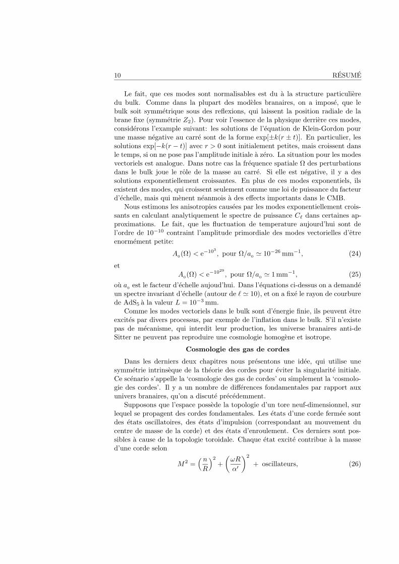
Le fait, que ces modes sont normalisables est du a la structure particulieredu bulk. Comme dans la plupart des modeles branaires, on a impose, que lebulk soit symmetrique sous des reflexions, qui laissent la position radiale de labrane fixe (symmetrie Z2). Pour voir l’essence de la physique derriere ces modes,considerons l’example suivant: les solutions de l’equation de Klein-Gordon pourune masse negative au carre sont de la forme exp[±k(r ± t)]. En particulier, lessolutions exp[−k(r − t)] avec r > 0 sont initialement petites, mais croissent dansle temps, si on ne pose pas l’amplitude initiale a zero. La situation pour les modesvectoriels est analogue. Dans notre cas la frequence spatiale Ω des perturbationsdans le bulk joue le role de la masse au carre. Si elle est negative, il y a dessolutions exponentiellement croissantes. En plus de ces modes exponentiels, ilsexistent des modes, qui croissent seulement comme une loi de puissance du facteurd’echelle, mais qui menent neanmois a des effects importants dans le CMB.
Nous estimons les anisotropies causees par les modes exponentiellement crois-sants en calculant analytiquement le spectre de puissance C` dans certaines ap-proximations. Le fait, que les fluctuation de temperature aujourd’hui sont del’ordre de 10−10 contraint l’amplitude primordiale des modes vectorielles d’etreenormement petite:
A0(Ω) < e−103
, pour Ω/a0' 10−26 mm−1, (24)
etA0(Ω) < e−1029
, pour Ω/a0 ' 1 mm−1, (25)
ou a0
est le facteur d’echelle aujoud’hui. Dans l’equations ci-dessus on a demandeun spectre invariant d’echelle (autour de ` ' 10), et on a fixe le rayon de courburede AdS5 a la valeur L = 10−3 mm.
Comme les modes vectoriels dans le bulk sont d’energie finie, ils peuvent etreexcites par divers processus, par exemple de l’inflation dans le bulk. S’il n’existepas de mecanisme, qui interdit leur production, les universe branaires anti-deSitter ne peuvent pas reproduire une cosmologie homogene et isotrope.
Cosmologie des gas de cordes
Dans les derniers deux chapitres nous presentons une idee, qui utilise unesymmetrie intrinseque de la theorie des cordes pour eviter la singularite initiale.Ce scenario s’appelle la ‘cosmologie des gas de cordes’ ou simplement la ‘cosmolo-gie des cordes’. Il y a un nombre de differences fondamentales par rapport auxunivers branaires, qu’on a discute precedemment.
Supposons que l’espace possede la topologie d’un tore neuf-dimensionnel, surlequel se propagent des cordes fondamentales. Les etats d’une corde fermee sontdes etats oscillatoires, des etats d’impulsion (correspondant au mouvement ducentre de masse de la corde) et des etats d’enroulement. Ces derniers sont pos-sibles a cause de la topologie toroidale. Chaque etat excite contribue a la massed’une corde selon
M2 =( nR
)2
+
(ωR
α′
)2
+ oscillateurs, (26)
11
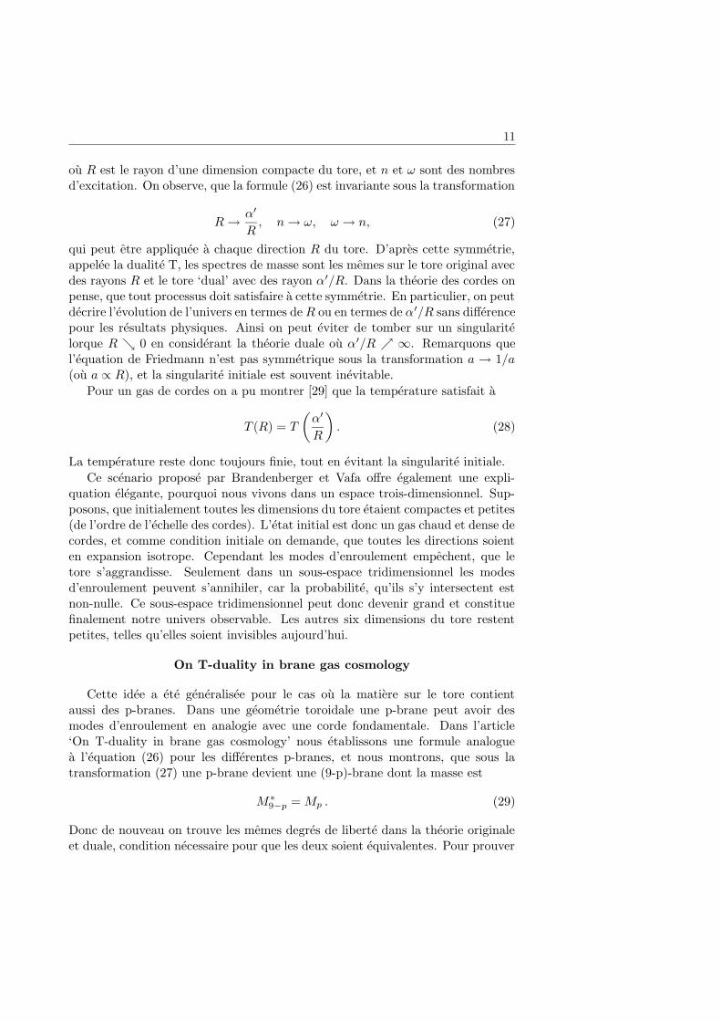
ou R est le rayon d’une dimension compacte du tore, et n et ω sont des nombresd’excitation. On observe, que la formule (26) est invariante sous la transformation
R→ α′
R, n→ ω, ω → n, (27)
qui peut etre appliquee a chaque direction R du tore. D’apres cette symmetrie,appelee la dualite T, les spectres de masse sont les memes sur le tore original avecdes rayons R et le tore ‘dual’ avec des rayon α′/R. Dans la theorie des cordes onpense, que tout processus doit satisfaire a cette symmetrie. En particulier, on peutdecrire l’evolution de l’univers en termes de R ou en termes de α′/R sans differencepour les resultats physiques. Ainsi on peut eviter de tomber sur un singularitelorque R 0 en considerant la theorie duale ou α′/R ∞. Remarquons quel’equation de Friedmann n’est pas symmetrique sous la transformation a → 1/a(ou a ∝ R), et la singularite initiale est souvent inevitable.
Pour un gas de cordes on a pu montrer [29] que la temperature satisfait a
T (R) = T
(α′
R
). (28)
La temperature reste donc toujours finie, tout en evitant la singularite initiale.
Ce scenario propose par Brandenberger et Vafa offre egalement une expli-quation elegante, pourquoi nous vivons dans un espace trois-dimensionnel. Sup-posons, que initialement toutes les dimensions du tore etaient compactes et petites(de l’ordre de l’echelle des cordes). L’etat initial est donc un gas chaud et dense decordes, et comme condition initiale on demande, que toutes les directions soienten expansion isotrope. Cependant les modes d’enroulement empechent, que letore s’aggrandisse. Seulement dans un sous-espace tridimensionnel les modesd’enroulement peuvent s’annihiler, car la probabilite, qu’ils s’y intersectent estnon-nulle. Ce sous-espace tridimensionnel peut donc devenir grand et constituefinalement notre univers observable. Les autres six dimensions du tore restentpetites, telles qu’elles soient invisibles aujourd’hui.
On T-duality in brane gas cosmology
Cette idee a ete generalisee pour le cas ou la matiere sur le tore contientaussi des p-branes. Dans une geometrie toroidale une p-brane peut avoir desmodes d’enroulement en analogie avec une corde fondamentale. Dans l’article‘On T-duality in brane gas cosmology’ nous etablissons une formule analoguea l’equation (26) pour les differentes p-branes, et nous montrons, que sous latransformation (27) une p-brane devient une (9-p)-brane dont la masse est
M∗9−p = Mp . (29)
Donc de nouveau on trouve les memes degres de liberte dans la theorie originaleet duale, condition necessaire pour que les deux soient equivalentes. Pour prouver
12 RESUME
l’absence d’une singularite initiale, il faudrait encore montrer, que la relation (28)est valable egalement pour un gas de p-branes.
Remarquons que dans la cosmologie des gas de branes nous ne vivons pas surune brane particuliere. Le role des branes est seulement de regler la dynamique del’espace-temps. En effet, en generalisant l’argument donne ci-dessus, nous avonsmontre, que le nombre de dimensions, qui deviennent ‘grandes’ est egalementtrois.
Dans les modeles des univers branaires, qu’on a etudie dans cette these, on atoujours trouve des instabilites dynamiques. Ceci indique, qu’il est tres difficilede construire une cosmologie valable avec ce genre de modeles. D’autre part,le scenario de la cosmologie des gas de branes offre une alternative interessante,meme s’il y a encore beaucoup de questions ouvertes. En comparant les deux, ilsemble finalement, que la cosmologie des gas de branes soit la plus prometteusepour unifier la theorie des cordes et la cosmologie.

Introduction
14 INTRODUCTION
Superstring theory is a fundamental theory, which unifies gravity and gauge in-teractions in a consistent and renormalizable way. The fundamental constituentsare no longer point-like particles, but 1-dimensional ‘strings’, whose oscillationsgive rise to a spectrum of particles. In particular, this spectrum contains a mass-less spin-2 state, which is identified with the graviton. It was also shown that thelow energy action of string theory reduces to the Einstein-Hilbert action of gen-eral relativity. Therefore, string theory includes gravity. At the same time, stringtheory gauge groups such as E8 contain SU(3)×SU(2)×U(1) as subgroups, andhence the standard model of particle physics can be accommodated.
For consistency requirements, such as Lorentz invariance and anomaly cancel-lation, superstring theory requires the number of space-time dimensions to be 10.It therefore predicts the existence of six spatial extra-dimensions. Certainly, thisis a logical possibility, which however has not been empirically verified until now.In fact, these extra-dimensions could be rolled up to small circles, such that theyare visible only at very high energies.
String theory also predicts the existence of (p+1)-dimensional hypersurfacesto which standard model fields are confined. An observer on such a ‘p-brane’would be able to notice the presence of extra-dimensions only by gravitationalinteractions, because gravity is the only fundamental force propagating in thewhole 10-dimensional space-time. Aside from the Einstein-Hilbert term, the lowenergy action of string theory contains also a number of new fields that are notpresent in the standard model, for instance the dilaton and the axion, which mayplay an important role in cosmology.
The idea of extra-dimensions has originally been introduced by Nordstrom,Kaluza, and Klein in order to unify gravity and electromagnetism. Many decadeslater, the development of supergravity theories led to a revival of this idea. Inthe framework of supergravity, the presence of seven additional dimensions isrequired, and p-branes arise naturally as classical solitonic solutions.
The significance of string theory for cosmology is that it can possibly resolvethe initial singularity (big bang) problem and, moreover, provide initial condi-tions. Therefore, it is important to investigate how string theory predictions suchas extra-dimensions and branes manifest themselves in a cosmological context.This is the principal aim of this thesis.
String theory is not supposed to modify the cosmological evolution from nu-cleosynthesis onward, where the physics are quite well understood and agree withobservations. But as a theory of quantum gravity, string theory is expected toplay an important role near the Planck scale. Stringy physics could have left animprint in the early universe and is probably necessary to understand it. On theother hand, one hopes to learn more about string theory through cosmologicalobservations.
The main body of this thesis consists of four articles corresponding to chap-ters 5, 7, 9, and 11. The published versions have been retained unchanged, apartfrom some adaptations of the notation for overall consistency. The purpose ofthe remaining chapters is to embed the research carried out in the literature that
15
already exists, as well as to provide a short introduction to each topic. Thesis estomnis divisa in partes tres4.
Part I: Extra-dimensions and branes
In part I we briefly review the standard cosmology, particularly emphasiz-ing issues which are of direct relevance for the present work. To start with,we point out the reason why string theory and supergravity require D = 10 orD = 11 space-time dimensions. Then, we work out the compactification of extra-dimensions in general, as well as on a torus and on an orbifold in particular. Ifextra-dimensions indeed exist, Newton’s law would get modified: in the presenceof n compact extra-dimensions, it would be a 1/r2+n law at scales much smallerthat the compactification radius. While the 4-dimensionality of gauge interactionshas been tested down to 1/200 GeV−1 ' 10−15 mm, Newton’s law is experimen-tally confirmed only above L ∼ 20µm, thus leaving room for new physics belowthat scale. This is an example where the scenario of extra-dimensions, and indi-rectly also sting theory, can be tested even in the laboratory.
Recently, it has been argued that relatively large compact extra-dimensions(i.e. with L ' µm) can solve the hierarchy problem: the effective 4-dimensionalNewton constant is given by G4 ∝ GD/L
n, where GD is the fundamental gravita-tional constant, which can be of the order of the electroweak scale so that, in thefundamental theory, the gap between the gravitational and the electroweak scaledisappears.
Part I is kept rather general and often goes somewhat beyond cosmology inorder to put our work into a broader context.
Part II: Brane cosmology
Part II is devoted to brane cosmology. Superstring theory and M theorysuggest that our observable universe could be a (3+1)-dimensional hypersurface,a 3-brane, embedded in a 10 or 11-dimensional space-time. This idea has recentlyreceived a great deal of interest. Such brane worlds have also been studied earlierin the context of topological defects, before branes were discovered to have astring theory realization.
A natural link between string theory and cosmology can be made within aframework called the mirage cosmology [90]. In this approach, our universe isidentified with a probe 3-brane moving in a higher-dimensional space-time, whichis given by a supergravity solution. If the bulk metric has certain symmetryproperties, the unperturbed brane motion leads to a homogeneous and isotropicexpansion or contration with a scale factor a(τ) on the brane. In the article ‘Per-turbations on a moving D3-brane and mirage cosmology’ in Chap. 5, we studythe evolution of perturbations on such a moving brane. Deviations from the un-perturbed embedding give rise to perturbations around the Friedmann-Lemaıtre
4C.Iuli Caesaris commentariorum de bello gallico, liber primus.
16 INTRODUCTION
solution, and those ‘wiggles’ can be directly related to the gauge invariant Bardeenpotentials. We show that on an expanding brane superhorizon modes grow as a4,while subhorizon modes are stable. On a contracting brane, both super- and sub-horizon modes are growing. These perturbations evolve as a consequence of thebrane motion only and are not sourced by matter. However, they are expected tobe important if matter is also included. Given the probe nature of the brane, ourmethod has many similarities with the study of topological defects. For example,the dynamics and perturbations are derived from the Dirac-Born-Infeld action,which is a generalization of the Nambu-Goto action. Therefore, it is not difficultto apply this method even when the number of co-dimensions is greater than one.On the other hand, we cannot include the back-reaction of the brane onto thebulk geometry, and this is a major shortcoming of the mirage cosmology.
In Chap. 6 and the following, we therefore investigate other brane world mo-dels, which accommodate the back-reaction via junction conditions linking the(real) energy content of the brane to the geometry of the bulk. This approachin turn is limited to the case of one co-dimension because, when there are morethan one extra dimensions, the junction conditions do not apply anymore. There-fore, much work has focused on the case in which our universe is a 3-brane in a5-dimensional bulk. This scenario is motivated by Horava-Witten compactifica-tion, where the brane is located at an orbifold fixed point. The bulk is in generaltime-dependent, and via the junction conditions this leads to a cosmological evo-lution on the brane. Binetruy et al. derived a Friedmann-like equation for thebrane world and showed, that the standard evolution can be recovered at latetimes [18]. A more general approach is to derive equations for the Einstein tensoron a 3-brane, which has been carried out by the authors of Ref. [142].
Randall and Sundrum proposed a bulk geometry in which the metric on the3-brane is multiplied by an exponentially decreasing ‘warp’ factor, such that trans-verse lengths become small at short distances along the fifth dimension [127]. Thisallows for a non compact extra-dimension without coming into conflict with obser-vational facts. A related model was proposed to solve the hierarchy problem [128].However, both models rely on a fine-tuning between the brane tension and thecosmological constant in the bulk. In the article ‘Dynamical instabilities of theRandall-Sundrum model’ in Chap. 7, we construct a dynamical generalization ofthe RS model, and show that, in a cosmological context, small deviations fromfine-tuning lead to runaway solutions. We also formulate a no-go theorem show-ing that the fine-tuning cannot be obtained by a dynamical mechanism involvinga scalar field or a fluid on the brane.
The next step is to derive observational consequences of brane world models.The cosmic microwave background (CMB) anisotropies represent some of themost important cosmological observations. Measurements of the temperaturefluctuations in the CMB provide us with a window on the early universe, and aretherefore also suited to confirm or rule out various brane world models. To thatend, a lot of work has been invested recently to derive gauge invariant perturbationtheory in brane worlds with one co-dimension [129].
17
In the article ‘CMB anisotropies from vector perturbations in the bulk’ inChap. 9, we take our universe to be a 3-brane moving in a 5-dimensional anti-deSitter (AdS5 ) bulk. The setup is similar to the one in the mirage cosmology,but this time the back-reaction is taken into account. We consider vector per-turbations in the bulk, which are modes of 5-dimensional gravity waves, and wefind analytically the most general solution of the perturbed Einstein equationsfor arbitrary initial conditions. Via the junction conditions, these bulk perturba-tions induce vector perturbations on the brane, and we find exponentially growingmodes, which are nonetheless perfectly normalizable. This differs radically fromthe usual behavior in the standard cosmology, where vector modes are alwaysdecaying. We estimate the effect on the angular power spectrum and discuss newsevere constraints for brane worlds.
Part III: Brane gas cosmology
In the last part, we present a scenario called brane gas cosmology. It is alsomotivated by superstring theory, but differs in many aspects from brane worldmodels. In particular, we are not thought to live on a brane, but rather in thebulk. The topology of the background space-time is that of a nine-torus, and thematter source consists of a gas of strings and p-branes.
Initially, all nine spatial dimensions are small and compact and, by a dynamicaldecompactification mechanism involving the winding modes of the strings andbranes, three dimensions grow large.
The main motivation which led to the development of brane gas cosmology isthe initial singularity problem in the standard cosmology. In their original work,Brandenberger and Vafa considered a gas of strings and showed that the T-dualitysymmetry of string theory can be used to give a singularity-free description of thecosmological evolution [29]. T-duality is a symmetry between large and smallscales, and it allows to describe the ‘region’ near the big bang in terms of lowcurvature scales. With this symmetry it can be shown that for a string gas thetemperature remained always finite in the past.
This idea was later extended to include various p-branes in addition to strings.In the article ‘On T-duality in brane gas cosmology’ in Chap. 11, we establishthe action of T-duality on the states making up the brane gas, and show thatthe mass spectrum is indeed invariant. Based on this, we claim that the initialsingularity can be avoided, also in the case that the matter source consists of agas of branes.
Notations and conventions
Unless explicitly mentioned, we shall use the following notations and conven-tions throughout this thesis:
• D denotes the total number of space-time dimensions, while d is the totalnumber of purely spatial dimensions, and n the number of extra-dimensions.Thus D = 1 + d = 1 + 3 + n.
18 INTRODUCTION
• M,N label coordinates of theD-dimensional space-time, µ, ν of a Lorentziansubmanifold (e.g. a brane), i, j of a Riemannian (mostly Euclidean) subma-nifold, and I, J of a Riemannian submanifold which represents the space ofextra-dimensions.
• It is often convenient to split the coordinates of the D-dimensional space-time as (xM) = (t, ~x, xI) = (t, xi, xI), where i = 1, · · · , p and I = p+1, · · · , d.In Chaps. 10 and 11 we write (xM) = (t, xn) where n = 1, · · · , d. If the focusis on a single extra-dimension xd, we shall write (xM) = (xµ, xd). In thecase D = 5 we set xd = y or xd = r.
• (σµ) = (τ, σi) = (τ, σ1, · · · , σp) denote internal coordinates on a submani-fold. On a brane, σ0 ≡ τ corresponds to cosmic time. In some places, weuse conformal time η instead.
• Boldface vectors are always 3-vectors, e.g. the direction of observation ofCMB photons is indicated by n.
• The metric of the D-dimensional space-time is GMN , and the induced orinternal metric on a Lorentzian submanifold is gµν . The two are related bya pull-back or push-forward. For clarity, we sometimes use a hat to stressthat a quantity is associated with gµν rather than with GMN . For example,
Rµνρσ is the induced (or internal) Riemann tensor on a brane.
• The metric signature is −+ · · ·+. The D-dimensional Minkowski metric is(ηMN) = diag(−1,+1, · · · ,+1).
• We use ≡ for definitions, ' for approximately equal, ∼ for a rough cor-respondence, and ∝ for a proportionality.
• MD denotes the D-dimensional (fundamental) Planck mass, and M4 theeffective Planck mass in our 4-dimensional universe.
• The D-dimensional cosmological constant is denoted by ΛD, and the cosmo-logical constant in our 4-dimensional universe by Λ4. As an exception weuse Λ instead of Λ5 for the 5-dimensional cosmological constant due to itsfrequent appearance.
We work in units ~ = c = kB = 1, such that there is only one dimension, energy,which is usually measured in GeV. Then,
[energy] = [mass] = [temperature] = [length]−1 = [time]−1.
Part I
EXTRA-DIMENSIONS ANDBRANES
19

Chapter 1
The cosmological standardmodel
22 CHAPTER 1. THE COSMOLOGICAL STANDARD MODEL
1.1 Isotropy and homogeneity of the observable uni-verse
The cosmological standard model relies on three main observations:
1. Isotropic expansion of the universe. In 1929 Hubble discovered thatthe spectra of most galaxies are redshifted and interpreted this as a Dopplershift1 resulting from their motion away from us (z = v/c). Furthermore, heobserved that the escape velocity of galaxies is proportional to their distance,v = Hd, where H is Hubble’s constant. The value of H today is 70 km
s·Mpc .
2. Isotropy of the cosmic microwave background (CMB) radiation.In 1965 Penzias and Wilson discovered a uniform background of ‘cosmicphotons’ corresponding to black body radiation of 3 K. In fact, in 1948Gamov had already predicted the existence of this radiation as left overafter the combination of electrons and protons into hydrogen during anearlier hotter phase of the universe. Since that moment the CMB photonshave travelled freely through the universe and have cooled down to theirpresent temperature of 2.725 K due to the cosmic expansion.
3. Abundance of light elements. The fact that high energies are needed tosynthesize elements gives another hint that the early universe must havebeen hot. (Formation in stars alone would not yield the correct abun-dances.) Nucleosynthesis calculations in the early universe predict the mea-sured abundances of hydrogen, helium, lithium, and deuterium. Nucleosyn-thesis also gives indirect evidence that the already the early universe musthave been very isotropic.
These three pieces of evidence tell us that our universe has emerged from a veryhot and dense state called the big bang. In general relativity, the big bang is an ini-tial singularity. During the subsequent expansion, the universe cooled down suchthat successively more and more structures (nuclei, atoms, molecules) could form.Small gravitational instabilities gave rise to the large scale structure observed to-day (solar system, galaxies, galaxy clusters). On scales above roughly 100 Mpc,the distribution of matter becomes isotropic2. Assuming that we do not inhabit apreferred position in space, we think of the whole universe as being homogeneouson large scales3. The dynamics of the expansion can then be described by highlysymmetric solutions of Einstein’s equations. They are called Friedmann-Lemaıtrespace-times (sometimes including also Robertson and Walker) after the Russianmathematician Alexander Friedmann, who in 1922 derived his cosmological equa-tions, and the Belgian priest Georges Lemaıtre, who is regarded as the father of
1In the framework of general relativity the red-shift is not interpreted as a Doppler shift, but asthe expansion of space-time itself.
2This is still small compared to the Hubble radius today, c/H0 = 3000h−10 Mpc.
3Nowadays, there are heated debates whether matter has a fractal distribution.
1.2. FRIEDMANN-LEMAITRE SPACE-TIMES 23
the big bang theory. We introduce this geometry in the next section (followingthe treatment of Ref. [149]).
1.2 Friedmann-Lemaıtre space-times
1.2.1 Isotropic manifolds
We start with the definitions of Riemannian and Lorentzian metrics and mani-folds.
Definition 1. A Riemannian metric on a differentiable manifold M is acovariant tensor field g of order two with the following properties:(i) g(X,Y ) = g(Y,X) ∀X,Y ∈ X (M), where X (M) is the set of all infinitelymany times differentiable vector fields on M.(ii) g is non degenerated at each point of M, i.e. if g(X,Y ) = 0 ∀Y =⇒ X = 0.(iii) The signature of g is (+, · · · ,+).
Definition 2. A pseudo-Riemannian metric satisfies (i) and (ii) of theabove definition, but the signature of g is (−, · · · ,−,+, · · · ,+).The special case (−,+, · · · ,+) is called a Lorentzian metric.
Definition 3. The pair (M, g) is called a Riemannian, pseudo-Riemannianor Lorentzian manifold according to the type of g defined above.
Isotropy is defined in the following way:
Definition 4. A 4-dimensional Lorentzian manifold (M, g) is isotropic with re-spect to the time-like velocity field v, g(v, v) = −1, if at each point q
Tqϕ |ϕ ∈ Isoq(M), (Tqϕ)v = v ⊇ SO3(v). (1.1)
Here, Tqϕ is the map between the two tangent spaces at the points q and ϕ(q)i.e. Tqϕ : TqM → Tϕ(q)M, and Isoq(M) is the group of local isometries of Mleaving the point q invariant. SO3(v) is the group of linear transformations inTqM leaving v invariant and inducing special orthogonal transformations in thespace orthogonal to v. Somewhat loosely speaking, definition (1.1) states that aspace-time is isotropic if the length and angle preserving maps with v invariantcontain the group of rotations. One can then show [148] that locally M can befoliated into a one-parameter family of spatial hypersurfaces Στ (with parameterτ) which are orthogonal to v. The integral curves of v are geodesics of (M, g),i.e. ∇vv = 0, and the geodesic distance between two hypersurfaces is constantindependent of q ∈ Στ . This allows to identify τ with a ‘cosmic time’. Further-more, one can prove that (Στ , γτ ) (where γτ is the induced metric on Στ ) is aspace of constant curvature. Then the map φ : Στ → Στ ′ induced by the flux φalong the integral curves of v satisfies φ∗γτ ′ = const ·γτ , where φ∗ is the pull-backassociated with φ. This means that, in comoving coordinates, the metric tensorson all hypersurfaces Στ are equal up to a ‘scale factor’.
24 CHAPTER 1. THE COSMOLOGICAL STANDARD MODEL
One may therefore decompose the metric tensor g on M as4
g = −dτ2 + a2(τ)γ, (1.2)
where dτ is a 1-form obtained by applying the exterior derivative d on the co-ordinate function τ , and γ is the metric of a 3-dimensional Riemannian spaceof constant curvature. The scale factor a depends only on the hypersurface andthus on τ . A space-time (M, g) with g given by Eq. (1.2) is called a Friedmann-Lemaıtre space-time. Notice that a manifold which is isotropic at each point q isalso homogeneous5.
We now investigate in more detail the Riemannian manifold (Στ , γτ ).
1.2.2 Riemannian spaces of constant curvature
In the following, we consider (Στ , γτ ) for some fixed value of τ and omit thesubscript. Let ∇ denote an affine connection on Σ, and X,Y, Z,W vector fieldsin X (Σ) ⊂ TqΣ. The curvature is the map
R :X (Σ)×X (Σ)×X (Σ) −→ X (Σ)
R(X,Y )Z = ∇X(∇YZ)−∇Y (∇XZ)−∇[X,Y ]Z.(1.3)
The last term vanishes in a coordinate basis. The Riemann tensor is defined via
R(X,Y, Z,W ) = g(X,R(Z,W )Y ), (1.4)
which is the scalar product of the two vectors X and R(Z,W )Y . Now let E ⊂ TqΣdenote an arbitrary plane in the tangent space TqΣ and X,Y two orthonormalvectors spanning E. For each plane E, the sectional curvature is defined by
Kq(E) = R(X,Y,X, Y ). (1.5)
Note, that this expression is independent of the basis of E.
Definition 5. If, for all points q ∈ Σ and for all planes E ⊂ TqΣ, the sectionalcurvature Kq(E) is equal to a constant K, then Σ is called a space of con-stant curvature. In the following, we consider K to be normalized, such thatK = +1, 0,−1 for positive, negative and zero curvature.
Spaces of constant curvature are frequently used also in brane cosmology, andwe shall discuss them in more detail in Sec. 2.4. In the next paragraph, we giveseveral coordinate expressions for Σ.
4Often g is also denoted by ds2.5A manifold (M, g) is called homogenous if locally g = −dτ 2 + γijdxidxj , in a coordinate basis
(τ, xi). The requirement of homogeneity is weaker than that of isotropy around each point.
1.3. THE GRAVITATIONAL FIELD EQUATIONS 25
1.2.3 The metric of Friedmann-Lemaıtre space-times
Let us introduce coordinates x1, x2, x2 on Σ. A basis of the co-tangent space T ∗q M
is then given by the 1-forms (dx0 ≡ dτ, dx1, dx2, dx3), and the metric tensor onM can be developed as
g =1
2gµν (dxµ ⊗ dxν + dxν ⊗ dxµ) ≡ gµν dxµdxν , gµν = gνµ. (1.6)
In a space of constant curvature one can always choose x1, x2, x3, such that themetric (1.2) takes the form
g = −dτ2 + a2(τ)1
(1 +K%2/4)2
[(dx1)2 + (dx2)2 + (dx3)2
], (1.7)
where %2 = (x1)2 + (x2)2 + (x3)2. Note that, unlike Σ, the manifold M is ingeneral not a space of constant curvature. On going to polar coordinates one has
(dx1)2 + (dx2)2 + (dx3)2 = d%2 + %2(dθ2 + sin2 θ dφ2), (1.8)
and by defining a new radial coordinate
r =%
1 +K%2/4, (1.9)
one can rewrite Eq. (1.7) in the form
g = −dτ2 + a2(τ)
[dr2
1−Kr2 + r2(dθ2 + sin2 θ dφ2)
]. (1.10)
Finally, we can substitute
r =
sinχ K = +1,χ K = 0,sinhχ K = −1,
(1.11)
to get the form
g = −dτ2 + a2(τ)[dχ2 + Σ2(χ)(dθ2 + sin2 θ dφ2)
], (1.12)
where
Σ2(χ) =
sin2 χ K = +1,χ2 K = 0,
sinh2 χ K = −1.
(1.13)
1.3 The gravitational field equations
In general relativity the metric gµν is a dynamical variable describing the gravi-tational field. Its dynamics are governed by Einstein’s equations
Rµν −1
2gµνR+ Λ4gµν ≡ Gµν + Λ4gµν = κ2
4Tµν , (1.14)
26 CHAPTER 1. THE COSMOLOGICAL STANDARD MODEL
which relate the energy-momentum tensor Tµν to the curvature of space-timeencoded in the Einstein tensor Gµν . The latter is a combination of the Riccitensor Rµν and the Riemann scalar R. The strength of the coupling is given bythe constant κ2
4, which is related to the Planck mass M4 and the Newton constantG4 by
κ24 =
1
M24
= 8πG4. (1.15)
This is the only free parameter in general relativity. Finally, the quantity Λ4 isthe cosmological constant.
1.3.1 Cosmological equations
From the gravitational field equations (1.14) one can derive cosmological equa-tions. This is most readily done in an orthonormal basis
ω0 = dτ, ωi =a(τ)
1 +K%2/4dxi. (1.16)
Then the components of the Einstein tensor, constructed from the Friedmannmetric (1.7), read
G00 = 3
(a2
a2+Ka2
),
G11 = G22 = G33 = −2a
a− a2
a2− Ka2,
(1.17)
where the dot denotes a derivative with respect to cosmic time τ .On scales where the universe is isotropic and homogeneous (& 100 Mpc), mat-
ter can be regarded as a continuous medium, and we assume this to be a perfectfluid. In the basis (1.16) the energy-momentum tensor then takes the form
T00 = ρ, Tij = Pδij . (1.18)
With these expressions, the 00 component of (1.14) leads to the first Friedmannequation
a2
a2+Ka2
=8πG4
3ρ+
Λ4
3, (1.19)
giving the expansion rate a of the universe as a function of its energy content,the spatial curvature and the cosmological constant. It is a first order differentialequation, because the 00 Einstein equation is a constraint.
One defines the Hubble parameter by
H =a
a, (1.20)
in analogy to the Hubble constant, which is the ratio v/d. In general, H dependson time.
1.3. THE GRAVITATIONAL FIELD EQUATIONS 27
From the 11 component of Einstein’s equations, and by using Eq. (1.19), oneobtains the second Friedmann equation
a
a= −4πG4
3(ρ+ 3P ) +
Λ4
3. (1.21)
Notice that Eqs. (1.19) and (1.21) are relations between measurable quantitiesand must therefore be independent of the basis or of the metric signature.
1.3.2 Energy ‘conservation’
The Einstein tensor satisfies geometrical identities
∇νGµν = 0, (1.22)
which are called contracted Bianchi identities. Via Einstein’s equations and forΛ4 = 0, one has
∇νTµν = 0. (1.23)
This is, however, not an energy conservation law, as it is not of the form ∂νTµν =
0. Indeed, this non conservation is due to the fact that matter exchanges energywith the gravitational field. But for the gravitational field there is no energy-momentum tensor: at any point q ∈ M, it can be transformed away, as locallygµν(q) = ηµν and Γµ
νλ(q) = 0, and without field there is no energy nor mo-mentum. Notice also that in special relativity the conservation laws for energyand momentum are based on the invariance of a closed system under translationsin space and in time. On a curved manifold, however, such translations are ingeneral not symmetries anymore, and therefore there exists no general energy-conservation law in general relativity6
For the Friedmann-Lemaıtre metric (1.7), the ν = 0 component of Eq. (1.23)yields
ρ+ 3H(ρ+ P ) = 0 (1.24)
giving the local rate of change of the energy density in a Friedmann-Lemaıtrespace-time. This equation is nevertheless called ‘the energy conservation law’.
The three equations (1.19), (1.21), and (1.24) are the basic equations gov-erning the dynamics of a Friedmann-Lemaıtre universe. Only two of them areindependent. For example, by using the ‘conservation’ law (1.24), the secondorder equation (1.21) can be integrated to obtain the first order equation (1.19).
1.3.3 Past and future of a Friedmann-Lemaıtre universe
Without solving explicitly the Friedmann equations, we can already make somequalitative statements about the dynamics of a Friedmann-Lemaıtre universe.Consider Eq. (1.21) with Λ4 = 0. As long as ρ+3P is positive, a must be negative.
6If however a Killing field K exists, i.e. a field satisfying LKg = 0, one can construct conservedquantities T µνKν , provided that Eq. (1.23) holds.
28 CHAPTER 1. THE COSMOLOGICAL STANDARD MODEL
Since the scale factor a is positive, and a is positive (due to the observed Hubbleexpansion), a(τ) is a concave function of τ . Therefore, a must have been zero atsome finite time in the past. This singularity of the Friedmann-Lemaıtre universecorresponds to the big bang. From equation (1.19) one can show, using similararguments, that when Λ4 = 0 the future behavior is entirely determined by thecurvature of the spatial sections. For K = −1 and K = 0 the universe expandseternally, while for K = +1 the expansion stops and turns into a contraction. Thefinal fate of the universe is then a ‘big crunch’ singularity where again a = 0.
Alternatively, the qualitative behavior can be obtained by specifying the en-ergy density ρ with respect to a critical energy density ρc. For Λ4 = 0 theFriedmann equation (1.19) yields
ρ =3
8πG4
(H2 +
Ka2
). (1.25)
The spatial curvature K is positive or negative, according to whether ρ is greateror less than the critical density
ρc ≡3H2
8πG4. (1.26)
Therefore, the universe eternally expands for ρ ≤ ρc and collapses for ρ > ρc.The value of ρc today is
ρc = 1.88 · 10−29 h20
g
cm3, H0 = 100h0
km
s ·Mpc, h0 = 0.70, (1.27)
where H0 denotes the Hubble parameter today.
It is useful to measure energy densities in terms of the critical energy densityby introducing the dimensionless parameter
ΩX =ρX
ρc, (1.28)
where X labels a particular contribution or particle species. Here, X will referto the curvature K or to the cosmological constant Λ4, and it will be omitted forthe usual matter density ρ. To write to the Friedmann equation in terms of ΩX ,we divide equation (1.19) by H2,
1 = − Ka2H2
+8πG4
3H2︸ ︷︷ ︸=
1
ρc
ρ+8πG4
3H2︸ ︷︷ ︸=
1
ρc
Λ4
8πG4︸ ︷︷ ︸=ρΛ4
, (1.29)
where we now have included Λ4 and attributed an energy density ρΛ4 to it, suchthat finally
1 = ΩK + Ω + ΩΛ4 . (1.30)
1.3. THE GRAVITATIONAL FIELD EQUATIONS 29
This form of the Friedmann equation is particularly useful for cosmological pa-rameter estimation.
Let us remark here, that the qualitative behavior of cosmological models isoften determined by rather general requirements on the energy-momentum tensorTµν , without need to specify a particular matter model. Consider, for example,matter satisfying (
Tµν −1
2gµνT
)vµvν ≥ 0, (1.31)
where v is an arbitrary unit time-like 4-vector and T = Tµνgµν is the trace of
the energy-momentum tensor. For a perfect fluid this corresponds to ρ+3P ≥ 0.The condition (1.31) is called strong energy condition. Via Einstein’s equations(for Λ4 = 0),
Rµν = κ24
(Tµν −
1
2gµνT
), (1.32)
the strong energy condition is equivalent to
Rµνvµvν ≥ 0⇐⇒ Ric(v, v) ≥ 0. (1.33)
Now, if the Ricci tensor of a manifold (M, g) satisfies this condition, one can provethat, a finite time back in the past,M is geodesically incomplete, and hence theremust have been an initial singularity (for a textbook treatment of these so-calledsingularity theorems see e.g. [160]).
It is however likely that Einstein’s equations do not hold near the singularity,and then the strong energy condition (1.31) does not translate into the condi-tion (1.33) for the singularity theorems7
Let us mention that there exists also a ‘weak energy condition’, Tµνvµvν ≥ 0,
which means that the energy density of matter as measured by an observer with4-velocity vµ has to be greater or equal than zero. For a perfect fluid, this amountsto ρ ≥ 0. Finally, the ‘dominant energy condition’ requires that −T µ
νvν be a
future directed time-like or null vector. Physically, this quantity corresponds tothe energy-momentum 4-current density of matter as seen by an observer withvelocity v. For a perfect fluid, this reduces to ρ ≥ |P |.
1.3.4 Cosmological solutions
The cosmological equations (1.19), (1.21), and (1.24) can be easily integrated,when the pressure is related to the energy density by an equation of state P = ωρ.First, the energy ‘conservation’ law (1.24) gives
ρ = ρi
(ai
a
)3(1+ω)
, (1.34)
7In fact, one of the main motivations to introduce stringy physics in cosmology is to avoid theinitial singularity. We are presenting a possibility to resolve the singularity problem in the article‘On T-duality in brane gas cosmology’ in Chap. 11.
30 CHAPTER 1. THE COSMOLOGICAL STANDARD MODEL
where ai and ρi are determined by the initial conditions. In the following we takethem to be the values today, ai = a0. In the matter dominated era one has ω = 0and ρ ∼ a−3, whereas in the radiation dominated era ω = 1/3 and ρ ∼ a−4.The extra factor a−1 is due to the stretching of wavelengths during the cosmicexpansion.
Let us assume that K = 0 and Λ4 = 0, and integrate the Friedmann equa-tion (1.19) by inserting the solution (1.34) for ρ. This leads to the relation
H2 = H20
(a0
a
)3(1+ω)
(1.35)
with H20 = 8πG4
3 ρ0. Eq. (1.35) is solved by
a
a0=
[(ai
a0
) 32 (1+ω)
+3
2(1 + ω)H0(τ − τi)
] 23(1+ω)
, (1.36)
where τi is some initial time, and ai = a(τi). For ω = 0, a ∼ τ 2/3, whereas forω = 1/3, a ∼ τ1/2. It will be interesting to compare these solutions with thoseobtained in brane cosmology in paragraph 6.3.3.
1.3.5 A remark on conformal time
Sometimes it is convenient to work with a different time coordinate, namely con-formal time η, defined via
g = −dτ2 + a2(τ)γ
≡ a2(η)(−dη2 + γ).(1.37)
The Hubble parameter in conformal time is
H =a′
a= Ha, (1.38)
where the prime denotes a derivative with respect to η. The Friedmann equa-tions (1.19) and (1.21) take the form
H2 +K =8πG4
3a2ρ+
a2Λ4
3, (1.39)
H′ = −4πG4
3a2(ρ+ 3P ) +
a2Λ4
3, (1.40)
and the energy ‘conservation’ law is
ρ′ + 3H(ρ+ P ) = 0. (1.41)
The relation corresponding to Eq. (1.35) is
H2 = H20
(a0
a
)1+3ω
, (1.42)
1.4. THE COSMIC MICROWAVE BACKGROUND 31
and the solution to that equation is
a
a0=
[(ai
a0
) 12 (1+3ω)
+1
2(1 + 3ω)H0(η − ηi)
] 21+3ω
. (1.43)
Here, ηi is some initial time and ai = a(ηi). For ω = 0, one has a ∼ η2, and forω = 1/3, one has a ∼ η.
1.4 The cosmic microwave background
At the beginning of this chapter we mentioned that small gravitational fluctua-tions in the early universe gave rise to the formation of large scale structures.Similarly, small perturbations in the matter density at the time when the universewas 300000 years old, result in temperature fluctuations in the cosmic microwavebackground (CMB) radiation today. Since those fluctuations are of the order of10−5, the universe must have been very isotropic at the age of 300000 years.
In this section, we give a brief description of the origin of the CMB. Historically,its existence was predicted by Gamov in 1946 and was confirmed by Penzias andWilson in 1965, providing strong support for the idea of a hot and dense beginningof the universe.
In a hot and dense initial phase of the universe, the photons were tightlycoupled to baryons and leptons, for example by Thompson scattering8 and othercollision processes. Thereby, the baryons play the role of the ‘walls of a cavity’with temperature T . Consequently, the spectral distribution of the photons isthat of black body radiation with temperature T .
When T has dropped to about 3000 K (corresponding to an age of 300000years) the electrons can combine9 with protons to form hydrogen atoms, andthe free electron fraction suddenly drops below 10−4. Consequently, the photon-electron interaction rate, Γ ∼ neσT , (ne is the free electron density, and σT isthe Thompson cross section) becomes small compared to the expansion scale,Γ¿ H, and the photons propagate freely through the universe. Conventionally,one defines a ‘last scattering surface’ by the condition ne = 1/2 (rather than someconstant time parameter).
During the subsequent cosmic expansion, the photons maintain their blackbody spectrum, but their temperature decreases according to T ∼ a−1 from3000 K down to 2.73 K. The spectrum observed today is the most perfect blackbody spectrum ever measured. Since its maximum is at micrometer wavelengths,the ensemble of photons is called cosmic microwave background. Because thosephotons have hardly interacted since their moment of emission, the CMB providesus with an image of the universe when it was 300000 years old,
8the scattering between photons and non relativistic electrons9Almost universally, the term ‘recombine’ is used, which is however misleading: the combination
happens just once.
32 CHAPTER 1. THE COSMOLOGICAL STANDARD MODEL
If the universe was completely isotropic at last scattering, photons incidentfrom different direction in the sky would have exactly the same temperature.However, this is not quite the case: various experiments have measured smalltemperature fluctuations in the CMB, called CMB anisotropies. The provide uswith rich information on cosmological parameters. We establish the link betweenmatter perturbations and CMB anisotropies in Chap. 8, and apply this formalismto anti-de Sitter brane worlds in Chap. 9.
1.5 Appendix
In this appendix, we fix our conventions (following [150] and [111]), in particu-lar those for the Riemann and Ricci tensors, as they are often a source of signconfusion. Let (M, g) be a 4-dimensional Lorentzian manifold and let
x :U ⊂M −→ V ⊂ R4
p ∈ U 7−→ xµ(p) ∈ V, with q 7−→ 0(1.44)
be a map from an open neighborhood U of q ∈M to an open neighborhood V ofzero in R
4. The set (xµ) = (x0, x1, x2, x3) are the coordinates of the point q. Abasis of the tangent space T0R
4 is given by the derivations
(∂µ) =
(∂
∂x0,∂
∂x1,∂
∂x2,∂
∂x3
), (1.45)
and a basis of the co-tangent space T ∗q M is given by the 1-forms
(dxµ) = (dx0, dx1, dx2, dx3). (1.46)
Since TqM is isomorphic to T0R4, the vectors (1.45) are also a basis of TqM, and
analogously for the co-tangent space.Let∇ denote an affine connection onM. The link with the covariant derivative
∇δ in the direction ∂δ is
(∇X)(dxγ , ∂δ) = 〈dxγ ,∇δX〉, (1.47)
where X ∈ TqM and 〈 〉 denotes the contraction. Notice that ∇X is a 1-times co-variant and 1-time contravariant tensor, whereas∇γX is a vector. The connection1-forms ωα
β and the Christoffel symbols Γαβδ are defined by
∇δ∂β = ωαβ(∂δ)∂α = Γα
βδ∂α, (1.48)
thus measuring the ‘twist’ of the basis vectors as they are transported on thecurved manifoldM. The Christoffel10 symbols are the coefficients of the connec-tion 1-forms
ωαβ = Γα
βγdxγ , (1.49)
10If the first index is downstairs (upstairs), they are called Christoffel symbols of the first (second)kind.
1.5. APPENDIX 33
because the basis (1.45) and (1.46) are dual to each other: 〈dxγ , ∂δ〉 = dxγ(∂δ) =∂δx
γ = δγδ . Furthermore, in the coordinate basis (1.45), the Christoffel symbols
can be expressed in terms of metric derivatives as
Γαβγ =
1
2gαλ(gλβ,γ + gλγ,β − gβγ,λ), (1.50)
where the subscript , γ is an abbreviation for the partial derivative ∂γ . Notice,that the Christoffel symbols are not components of some tensor.
We have already defined the curvature in Eq. (1.3) as well as the Riemanntensor in Eq. (1.4). The components of the Riemann tensor are
Rαβγδ = g(∂α, R(∂γ , ∂δ)∂β). (1.51)
Alternatively, this can be written as a contraction
Rαβγδ = 〈dxα, R(∂γ , ∂δ)∂β〉 = 〈dxα, (∇γ ∇δ∂β︸ ︷︷ ︸
=Γλβδ∂λ
−∇δ ∇γ∂β︸ ︷︷ ︸=Γλ
βγ∂λ
)〉
= Γαβδ,γ + Γλ
βδΓα
λγ − (γ ↔ δ),
(1.52)
where in the first line, we have used the fact that in a coordinate basis thecommutator [∂γ , ∂δ] vanishes. The Riemann tensor has the following symmetries(the square brackets denote antisymmetrization):
Rαβγδ = −Rβαγδ Antisymmetry in the first two indices,Rαβγδ = −Rαβδγ Antisymmetry in the last two indices,Rα[βγδ] = 0 Vanishing of antisymmetric parts,Rαβ[γδ;ε] = 0 Bianchi identity.
(1.53)
In the last equation, the semicolon denotes ∇ε. Eqs. (1.53) are the complete setof symmetries of the Riemann tensor. From these, one can deduce the additionalsymmetries
Rαβγδ = Rγδαβ Symmetry under pair exchange,R[αβγδ] = 0.
(1.54)
The Ricci tensor is defined as the contraction of the Riemann tensor on the firstand third (or second and fourth) indices,
Rβδ = gαγRαβγδ = Rαβαδ, (1.55)
and is symmetric in its indices. From Eq. (1.52), the Ricci tensor in terms of theChristoffel symbols reads
Rβδ = Γαβδ,α + Γλ
βδΓα
λα − Γαβα,δ − Γλ
βαΓαλδ. (1.56)
The extension of these definitions to a D-dimensional space-time is straightfor-ward. We shall need some of these expressions in Chap. 8, when we calculate theperturbed Einstein equations in an AdS5 background.

Chapter 2
Extra-dimensions
36 CHAPTER 2. EXTRA-DIMENSIONS
2.1 Motivation
The idea that a higher-dimensional approach may help to understand (3+1)-dimensional phenomena appeared several times in the history of physics. In thetwenties Theodor Kaluza [87] and Oskar Klein [94] proposed a 5-dimensional the-ory to unify gravity and electromagnetism. They observed that the 4-dimensionalgravitational and electromagnetic fields can be understood as components of thefive-dimensional metric tensor. Unfortunately, it turned out that the Kaluza-Klein mechanism is not a phenomenologically working theory, but it still servesas a prototype for many higher-dimensional models (see Sec. 2.5).
Until today, there is no experimental evidence for the existence of extra-dimensions. Nevertheless, theories with extra-dimensions were and are develo-ped, because a higher-dimensional approach is often useful to understand ‘un-connected’ phenomena from a more fundamental and unified perspective. Forinstance, the existence of extra-dimensions would opened up new possibilities toconnect particle physics and cosmology, as well as to answer questions on renor-malizability, the unification of forces, and the big bang singularity. Let us take acloser look at this, proceeding cronologically.
In the seventies an 11-dimensional theory called supergravity was constructed.Until then, all attempts to unify general relativity and quantum field theoryturned out to be non renormalizable. The hope in supergravity was that the di-vergence problems of quantum gravity theories could be solved if supersymmetryis added. The peculiar dimensionality ‘eleven’ arises, as it is the largest possi-ble number of space-time dimension (and thus incorporates the largest possiblesymmetry group) in which a consistent field theory can be constructed. However,these hopes were dashed when it became clear that local supersymmetry is notenough to overcome the divergence problems. Nevertheless, supergravity remainsimportant since it was discovered, later on, to be the low energy limit of stringtheory. As the supergravity equations of motion are needed in the article ‘Pertur-bations on a moving D3-brane and mirage cosmology’ in Chap. 5, we introducethem in Sec. 2.2.
Nowadays the most promising theory of quantum gravity is string theory. Itsfundamental constituents are no longer point particles, but 1-dimensional objectscalled strings. They are characterized by a tension, and their excitations give riseto states representing various massless and massive particles, notably the graviton.Supersymmetric string theories require the number of space-time dimensions tobe ten. The success of string theory in unifying gravity and gauge interactionswithout divergences is the main reason today to take extra-dimensions seriously.Some basic ideas of string theory are presented in Sec. 2.3. In particular, it isdemonstrated how string theory predicts the number of space-time dimensions,and what the spectrum of a closed string looks like. The latter is relevant for thearticle ‘On T-duality in brane gas cosmology’ in Sec. 11.
In all these theories there is a number n of spatial extra-dimensions in additionto the observed three. One can think of this as attaching an n-dimensional space
2.2. SUPERGRAVITY 37
at each point of our 4-dimensional space-time. The total number of space-timedimensions is then D = 1 + d = 1 + 3 + n. In the previous examples: D = 5(Kaluza-Klein), D = 11 (supergravity), and D = 10 (superstring theory).
Why have these extra-dimensions not been observed (yet)? A simple expla-nation is that they could be curled up to small circles of the order of the Plancklength, and that therefore they are ‘visible’ only at energies near the Planck mass∼ 1019 GeV. There exist also scenarios in which this ‘compactifiaction scale’ isaround 1 TeV, such that it could be accessible in future collider experiments.
A rather intuitive explanation of this is the following: think of a thin andlengthy object, for example a pencil. If it is looked at from very far, the pencilappears as a 1-dimensional object, because the eye cannot discern the thickness.But looking from a small distance, the second rolled up dimension of the pencilbecomes visible. In physics, ‘looking close’ means ‘looking at high energies’, andtherefore compact extra-dimensions can only be seen at high-energies.
We make some general remarks about compact spaces in Sec. 2.4, and presenttwo specific types of compactifications, namely toroidal compactification andHorava-Witten compactification, in section 2.5 and in paragraph 2.5.3.
The presence of extra-dimensions would modify Newton’s law of gravitationalattraction. Instead of the F ∼ 1/r2 form, one finds that the force depends onthe number n of extra-dimensions according to F ∼ 1/r2+n. This is encouraging,for it allows to test the scenario of extra-dimensions in the laboratory withoutresorting to high energy experiments. A derivation of the modified Newton’s lawis given in Sec. 2.6.
Finally, in Sec. 2.7 we discuss an idea to solve the hierarchy problem with‘large’ extra-dimensions.
2.2 Supergravity
In general relativity the (local) symmetry group is the Poincare group. Thecorresponding set of generators can be extended to include supersymmetry trans-formations. One then obtains a classical field theory called supergravity. In orderto make the symmetry group as large as possible one tries to construct a the-ory with the highest possible number of space-time dimensions. This turns outto be eleven, since for D > 11 the spectrum contains massless particles of spingreater than two, and hence is inconsistent already on the classical level. There-fore, from a theoretical point of view, 11-dimensional supergravity is the ‘mostgeneral’ starting point for a unifying theory of gravity and gauge interactions.
Instead of the original 11-dimensional action of supergravity we shall writedown its form after a dimensional reduction to D = 10. We postpone explaininghow to do this until Sec. 2.5, and simply give the result here. The 10-dimensionalreduced supergravity action is particularly useful because supergravity is the lowenergy limit of type IIB super string theory. Obtaining one action from the otherby a simple dimensional reduction is possible as the supersymmetry algebras of
38 CHAPTER 2. EXTRA-DIMENSIONS
the two theories are the same.
The low energy action of type IIB superstring theory is1 [125]
S10 =1
2κ210
∫d10x√−Ge−2Φ
(R+ 4(∇MΦ)(∇MΦ)− 1
2
1
3!HABCH
ABC
)
− 1
2κ210
∫d10x√−G1
2
1
5!FABCDEF
ABCDE,
(2.1)
where κ210 is related to the 10-dimensional gravitational constant. The indices
are pulled up and down by the 10-dimensional metric GMN . The field Φ is thedilaton2, and the 3-form field strengthHABC derives from an antisymmetric tensorfield BMN via the exterior derivative H3 = dB2. The fields in the first line aremultiplied by a factor e−2Φ which is the inverse squared of the string couplingconstant gs. The power −2 corresponds to the coupling in a tree-level diagramin string theory. Furthermore, there is a 5-form field strength FABCDE associatedwith a 4-form potential CMNRS via F5 = dC4. The reason why this term isinteresting is that the 4-form naturally couples to a 3-brane3.
We are interested only in certain features of the low energy action that wewill use for cosmology, and for simplicity we have omitted a 1-form F1, a 3-formF3 as well as fermionic and Chern-Simons terms (gauge invariant terms wherewedge products of the p-form potentials appear rather that their derivatives).Notice that the high degree of supersymmetry (16 or 32 generators) completelydetermines the low energy action (2.1)4.
This action is written in the so-called string frame: compared to the usualEinstein-Hilbert action or the action for a scalar field, there is a unusual factore−2Φ and a wrong sign of the scalar field kinetic term. This can be changed bygoing to a physical frame called Einstein frame (labelled by an e) by a conformaltransformation
GeMN = Ω2GMN = e−
4ΦD−2GMN . (2.2)
Here D = 10, thus in the action (2.1) we have to replace GMN by e+Φ/2GeMN
which yields, for example
HABCHABC = He
ABCHABC
e e−3Φ/2, (2.3)
where the sub- or superscript e simply means that now the indices are pulled upand down with the metric in the Einstein frame. Under the conformal transfor-
1In the article in Chap. 5 we use the more compact notation∫
d10x√−G 1
5!FABCDEF ABCDE =∫
F ∧ ∗F for the second integral, where ∗F is the Hodge dual of F .2Physically, the dilaton measures the size of the eleventh compactified dimension.3It is well known that a 1-form, e.g. the electromagnetic potential Aµ, couples to the charge of
a point particle which is 0-brane. In analogy, a 2-form potential couples to a 1-brane or a string, a3-form potential couples to a 2-brane and so on.
4In string theory the action Eq. (2.1) corresponds to the low energy action of type IIB, and thefields in the first line, GMN , HABC , and Φ, are associated with the Neuveu-Schwarz (NS-NS) sector,whereas CMNRS with the Ramond-Ramond (RR-RR) sector.
2.3. STRING THEORY 39
mation (2.2) the Riemann scalar transforms as (see Ref. [160])
R = Ω2 [Re + 2(D − 1)GMN
e ∇M∇N lnΩ− (D − 2)(D − 1)GMN
e (∇M ln Ω)(∇N ln Ω)]
= e−Φ/2
[Re −
9
2GMN
e ∇M∇NΦ− 9
2GMN
e (∇MΦ)(∇NΦ)
],
(2.4)where R and Re are the Riemann scalars constructed from the metrics GMN andGe
MN respectively. The action written in the Einstein frame is
Se10 =
1
2κ210
∫d10x
√−Ge
(Re −
1
2(∇MΦ)(∇MΦ)− 1
2
1
3!e−ΦHe
ABCHABC
e
− 1
2
1
5!F e
ABCDEFABCDE
e
),
(2.5)
where the exponential is not present anymore, and the dilaton kinetic term comeswith the right sign and prefactor. We have used the fact that ∇M∇MΦ = 0 whichis the dilaton equation of motion if the source is a 5-form (see below).
This action is of great importance for brane cosmology, for it admits solutionswhich are extended objects, so-called p-branes (see Chap. 3). Cosmologists oftentend to use simplified effective theories in space-times with other dimensionalitiesthan ten, mostly four, five or six, and to keep only fields which they can makeuse of. Therefore let us generalize the action to a D-dimensional space-time, thefield strength to a q-form, and omit the field H3. We shall also suppress the sub-or superscripts e as now all quantities are in the Einstein frame
SD =1
2κ2D
∫dDx√−G
(R− 1
2(∇MΦ)(∇MΦ)− 1
2
1
q!eaqΦFA1···AqF
A1···Aq
),
(2.6)which leads to the equations of motion
RMN =1
2(∇MΦ)(∇NΦ)
+1
2
1
(q − 1)!eaqΦ
(FMA2···AqFN
A2···Aq − q − 1
q(D − 2)FA1···AqF
A1···AqGMN
),
0 = ∇M
(eaqΦFMA2···Aq
),
∇M∇MΦ =1
2
aq
q!eaqΦFA1···AqF
A1···Aq ,
(2.7)where aq = (5− q)/2.
2.3 String theory
2.3.1 Introductory remarks
Despite its great success, the SU(3)×SU(2)×U(1) standard model, together withgeneral relativity, is certainly not a complete description of nature. Firstly, the
40 CHAPTER 2. EXTRA-DIMENSIONS
standard model depends on roughly twenty free parameters and is therefore tooarbitrary. Secondly, attempts to unify quantum field theory with general relativityfollowing the usual perturbative methods have failed, because the theory turnedout to be non renormalizable. This indicates that at ‘high energies’ new elementscome into play. And thirdly, the singularities of general relativity survive even inthis unified theory.
A number of ways have been suggested to solve these problems. One ideais extra-dimensions, first suggested to unify electromagnetism and gravity. An-other idea is to include supersymmetry, which resulted in supergravity theories.However, none of these concepts have led to a theory that solves all of the prob-lems mentioned above. The first plausible and promising candidate for a workingtheory of quantum gravity is string theory.
From quantum field theory we are used to point-like particles that are excita-tions of some field and which interact locally by exchange of gauge particles. Instring theory the fundamental constituents are strings, i.e. 1-dimensional objects.Like a chord, a string can oscillate, and there is a spectrum of masses or energiesassociated with the different oscillatory states. To a low energy observer an oscil-lating string looks like a point-like particle with a rest mass equal to the energy ofthe oscillatory state. In particular, a single string can give rise to different typesof particles depending on its state of oscillation.
When building a consistent quantum theory based on strings one finds that:a) such a theory includes gravity: the spectrum contains a massless spin-2 state,the graviton, which arises as an excitation of a closed string. Moreover, theEinstein-Hilbert action of general relativity turns out to be part of the low energyaction of string theory. This is the ‘string theory miracle’. b) String theory isa consistent and divergence-free theory of quantum gravity. In particular, theultraviolet divergence, arising from short distances, is absent. Roughly speakingthis is due to the fact that extended objects such as strings ‘smear out’ theinteractions over space-time, and this softens the UV divergence. The technicalargument is that, when calculating string amplitudes, the UV divergent region isnot in the domain of integration. c) String theory gauge groups, e.g. E8, containthe standard model groups. d) A consistent string theory must be supersymmetric(called superstring theory), because bosonic string theory has a tachyon. Unlike inquantum field theory, fermions are now required for consistency. e) String theoryhas only one free parameter, α′ = 1/2πτF , where τF is the string tension5. Thissets the string length scale `s = α′1/2 and the string mass scale ms = α′−1/2. f)Superstring theory predicts the number of space-time dimensions to be D = 10.It requires the existence of extra-dimensions for consistency. Points a) and f)are particularly interesting for cosmology. If string theory really is the correctdescription of nature, one must ask the question how cosmology looks like withinthis framework.
There exist five types of superstring string theories, called type I, IIA, IIB,
5The subscript F indicates that it is a fundamental sting, in contrast to D-strings (1-branes) thatwe shall encounter later on, and to cosmic strings.
2.3. STRING THEORY 41
heterotic SO(32), and heterotic E8×E8. Type I is a theory of open and closed un-oriented superstrings, whereas type II contains only closed oriented superstrings.Here, I and II is the number of supersymmetry generators, and A and B indicatethat the left- and right-moving oscillators transform under separate space-timesupersymmetries that have opposite (A) or equal (B) chirality. These five stringtheories can be viewed being different corners in the moduli space of a single the-ory, called M theory6. A particular compactification of M theory due to Horavaand Witten is highly relevant for brane world models. We shall discuss it inparagraph 2.5.3.
It would be beyond the scope of this thesis (and the knowledge of its author) toenter into more details here. In the following sections, however, we shall discuss insome detail the string theory prediction of the space-time dimensionality, as wellas the mass spectrum of a closed string, since these issues are of direct relevancefor the articles in this thesis.
2.3.2 10- and 26-dimensional space-times
In general relativity, space-time is a given fundamental quantity, whose dynamicsare described by Einstein’s equations. The number of space-time dimensions is setto four by hand. In string theory space-time is a derived concept: the fundamentalquantity is the world-sheet W, swept out by a moving string, and the dynamicsare described by the Polyakov action
S = − 1
4πα′
∫
Wdτdσ
√−g gµν(∂µXM)(∂νX
N)GMN . (2.8)
Here, τ and σ are internal coordinates on the world-sheet with −∞ < τ <∞, 0 ≤ σ ≤ s, where s is the length of a string, and gµν (with µ = τ, σ) isthe internal metric. Diffeomorphism invariance on W requires that X ′M(τ ′, σ′) =XM(τ, σ). Therefore, from the world-sheet perspective, the set XM correspondsto D massless scalar fields covariantly coupled by the metric GMN (setting M =0, · · · , D − 1). On W everything can be described in terms of a 2-dimensionalconformal field theory. On the other hand, one may want to embed the world-sheet into a D-dimensional target space-timeMD. Then, XM(τ, σ) play the roleof embedding functions. A priori we do not know, what properties MD shouldhave for the theory to be consistent, so for the moment we must leave the valueof D open. Now here is the crucial point: specifying the ‘couplings’ of the Dscalar fields to each other is equivalent to specifying GMN . Therefore, space-timeis encoded in a 2-dimensional conformal field theory, and string theory is ableto predict its dimensionality. It is D = 26 for bosonic strings, and D = 10 forsuper strings. Since there is no intuitive explanation of this result, and since it iscrucial for brane cosmology, we would like to present a short calculation following
6Much about M theory is yet obscure, and also concerning its name there are only guesses whether‘M’ stands for matrix, membrane, mother, mystery, magic, or is an inversed ‘W’ for Witten.
42 CHAPTER 2. EXTRA-DIMENSIONS
Ref. [124] to assert this prediction. For simplicity, the demonstration is made foropen bosonic strings.
We use light cone coordinates7 xM = (x+, x−, xi) where x± = (x0 ± x1)/√
2,i = 2, · · · , D − 1, and the canonical momenta are denoted pM = (p+, p−, pi).The aim is to determine D. The position of a point on the string is given byxM = XM(τ, σ), and the transverse embedding functions X i satisfy the waveequation8
∂2τX
i = c2∂2σX
i, (2.9)
with velocity c = s/2πα′p+. We impose Neumann boundary conditions by re-quiring that the derivative tangential to the string vanishes (‘no momentum isflowing off the string’): ∂σX
i = 0 at σ = 0, s. Then the general solution toEq. (2.9) is9
Xi(τ, σ) = xi +pi
p+τ + i(2α′)1/2
∑
n6=0
αin
ne−iπncτ/s cos
(πnσs
), (2.10)
where the sum runs over all n from minus infinity to plus infinity, except forn = 0. In fact, the n = 0 term corresponds to the center of mass momentum ofthe string10
pi(τ) =p+
s
∫ s
0
dσ ∂τXi(τ, σ), (2.11)
whereas the first term is center of mass position
xi(τ) =1
s
∫ s
0
dσXi(τ, σ). (2.12)
Each oscillator mode n has an amplitude αin which, upon quantization, becomes
an operator satisfying the bosonic commutation relations
[αim, α
jn] = mδijδm,−n (2.13)
for each i, j, n,m separately. The requirement that X i be real leads to (αin)† =
αi−n. The Hamiltonian is [124]
H =1
2p+
D−1∑
i=2
pipi +1
4p+α′
( ∞∑
n=1
D−1∑
i=2
αi−nα
in + αi
nαi−n
). (2.14)
Note that creation and annihilation operators are not yet normal ordered. Byusing the commutation relations (2.13) for m = n and summing over the D − 2
7By using light cone coordinates, the diffeomorphism and Weyl redundancy of the Polyakov actionis eliminated.
8After a particular gauge fixing of the induced metric on the world-sheet.9This solution extends to X+ and X−, but for our purpose only the transverse coordinates are
relevant.10The exact definition of p+ is made via the Lagrangian of the string, see Ref. [124]. Here, we
content ourselves with the observation that p+ corresponds to the energy of the string.
2.3. STRING THEORY 43
transverse coordinates, one finds
D−1∑
i=2
αinα
i−n =
D−1∑
i=2
αi−nα
in + n(D − 2). (2.15)
Upon inserting this into Eq. (2.14) one encounters an infinite sum over all n whichcan be regularized to give
∞∑
n=1
n = − 1
12. (2.16)
Thus the Hamiltonian becomes
H =1
2p+
D−1∑
i=2
pipi +1
2p+α′
( ∞∑
n=1
D−1∑
i=2
αi−nα
in +
2−D24
). (2.17)
The mass squared of an oscillatory state is now
M2 = 2p+H −D−1∑
i=2
pipi =1
α′
(N +
2−D24
), (2.18)
where we have replaced the sum over the oscillators by the level number N . Letus look at the first excited state with N = 1
αi−1|0〉, M2 =
1
α′26−D
24. (2.19)
Since i runs form 2 to D − 1, these are D − 2 internal states. This is exactly theamount of states that a massless spin 1 particle has in a D-dimensional space-time. This comes as follows: for a massless particle the momentum can be writtenas pM = (E,E, 0, · · · , 0), hence the invariance group is the little group SO(D−2).Now the spin 1 representation of SO(D−2) is (D−2)-dimensional, giving rise toD− 2 internal states. Therefore the state (2.19) must be massless which requiresD = 26. Summarizing, by simply demanding Lorentz invariance, we have foundthat the bosonic string can only live in a target space-time that has 1 time and25 spatial dimensions. A similar argument, including fermionic fields, shows thatfor superstrings the number of space-time dimensions must be D = 10.
These predictions, which appear to be wrong at first sight, are usually rec-onciled with the observed D = 4 by compactifying the superfluous dimensions(see Sec. 2.5). But here is the problem: the effective 4-dimensional theory, andconsequently the physical constants in our universe, crucially depend on the de-tails of the compactification process. Therefore, string theory looses virtuallyall of is predictive power. It is not clear how to overcome this deficiency. InChap. 10 we discuss a dynamical ‘decompactification’ mechanism which possiblyhelps avoiding the problem.
44 CHAPTER 2. EXTRA-DIMENSIONS
2.3.3 Mass spectrum of a closed string on a compact direction
In preparation for part III of this thesis, we derive the mass spectrum of a closedstring put on a compact direction. We shall encounter momentum, winding, andoscillatory modes which are interesting for string and brane gas cosmology.
A closed string solution of the wave equation (2.9) has to satisfyXM(τ, σ+s) =XM(τ, σ), in addition to the Neumann boundary condition. The mode expansionis now
XM(τ, σ) = xM+pM
p+τ+i
(α′
2
)1/2∑
n6=0
(αM
n
ne−2πn(icτ+iσ)/s +
αMn
ne−2πn(icτ−iσ)/s
).
(2.20)We have replaced the index i byM , as allD space-time coordinates solve Eq. (2.9).It is easy to see that Eq. (2.20) is the correct mode expansion for the closedstring by comparing it with the form (3.68) of the open string solution11. Inboth cases the first term of the oscillatory part corresponds to a left moving waveand the second to a right moving wave. On a closed string, those modes travelindependently in opposite senses. Therefore, the two amplitudes αM
n and αMn are
different, whereas for the open string they are tied together by the Neumannboundary condition. Notice also that there is a factor 2π instead of π in theexponent to satisfy the periodicity condition mentioned above.
One may rewrite Eq. (2.20) in terms of complex coordinates z = eσ0+iσ andz = eσ0−iσ, where σ0 = icτ becomes real after an analytic continuation to aMinkowskian world-sheet. In the momentum term, τ can be expressed as τ =ln(|z|2)/(2ic). The length of the closed string is set to be s = 2π. Then thevelocity defined under Eq. 2.9 becomes c = 1/(α′p+). With these substitutionsEq. (2.20) reads
XM(z, z) = XM(z) +XM(z)
=
x
M
2− iα
′
2pM
L ln(z) + i
(α′
2
)1/2∑
n6=0
αMn
nz−n
+
x
M
2− iα
′
2pM
R ln(z) + i
(α′
2
)1/2∑
n 6=0
αMn
nz−n
.
(2.21)
We have split the center of mass momentum pM into left and right moving mo-menta pM
L and pMR , in order to write the mode expansion as a sum of two in-
dependent parts: the ‘left-movers’ are described by a holomorphic function, the‘right’movers’ by an anti-holomorphic function.
Let us focus for a moment on the zero modes. From Eq. (2.21) one finds,substituting back τ and σ,
XM(τ, σ) = xM +α′
2(pM
L + pM
R ) cτ +α′
2(pM
L − pM
R )σ. (2.22)
11which is just a rewriting of the open string mode expansion given in Eq. (2.10)
2.3. STRING THEORY 45
In a non compact space-time the embedding functions are single valued and, asone runs around the closed string, XM(τ, σ + 2π) = XM(τ, σ). Thus pM
L = pMR ,
and Eq. (2.22) is just a trivial rewriting of Eq. (2.20). Suppose now that onedirection, xd say, is a circle of radius R. Then
Xd(τ, σ + 2π) = Xd(τ, σ) + 2πRω, (2.23)
where 2πR is the periodicity, and ω ∈ Z. This leads to the constraint
α′
2
(pd
L − pdR
)= ωR. (2.24)
On the other hand, the momentum flowing around a compact direction must bequantized according to12
pdL + pd
R =nL
R+nR
R=
2n
R, nL, nR, n ∈ Z. (2.25)
From Eqs. (2.24) and (2.25) one finds
pdL =
n
R+ωR
α′ , pdR =
n
R− ωR
α′ . (2.26)
Momentum along a compact direction looks like mass in the remaining D − 1dimensions (see Eq. (2.47) later on). Intuitively, the momenta in Eq. (2.26) givetherefore rise to an ‘averaged’ mass
M2 ' 1
2
[(pd
L
)2+(pd
R
)2]=( nR
)2
+
(ωR
α′
)2
. (2.27)
More carefully, one requires that the Virasoro generators13 L0 and L0 vanish
0 = L0 =1
2
α′
2
[(pd
L
)2+ p2
]+N − 1,
0 = L0 =1
2
α′
2
[(pd
R
)2+ p2
]+ N − 1,
(2.28)
where p2 denotes the space-time momentum in the D−1 non compact dimensions.N and N are the total level number of left- and right-movers, and −1 is a constantfrom normal ordering the expressions. The D − 1-dimensional mass is given byM2 = −p2. Inserting expressions (2.26) into (2.28) and solving for M 2 yields
M2 =( nR
)2
+
(ωR
α′
)2
+2
α′ (N + N − 2). (2.29)
12This can be seen as follows: the general translation operator is exp(ixdpd). Under a full transla-tion around the compact direction, i.e. xd = 2πR, a state must be invariant. Thus exp(i2πRpd) = 1,and hence pd = n/R, where n ∈ Z.
13A profound explication would be beyond the scope of this thesis. Here, we just remark that theVirasoro generators are coefficients of the Fourier expansion of the energy-momentum tensor on theworld-sheet of a string. The requirement that L0 = 0 and L0 = 0 for left- and right-movers is aphysical state or on-shell condition.
46 CHAPTER 2. EXTRA-DIMENSIONS
Eq. (2.29) is the main result of this section. It shows how momentum-, winding-,and oscillatory modes contribute the mass of a closed string. Notice that thecontribution of the oscillators is set by the string tension which is proportional to1/α′. The number ω is a winding number, counting how many times the stringwinds around the compact direction. It is positive or negative according to theorientation of the string. Two states with opposite winding ±ω may annihilate,leaving a state with ω = 0. Strings with non zero winding number are topologicalsolitons. The existence of winding states is an intrinsically stringy phenomenon.
Furthermore, it can be shown that the combination L0 − L0 generates trans-lations along the string. Hence, one requires additionally that L0 − L0 = 0 toensures that the physics remain invariant. Subtracting the two equations in (2.28)leads to the ‘level matching condition’
nω +N − N = 0. (2.30)
If there are equally many left and right moving oscillators, either the center ofmass momentum along the string or the winding number have to be zero. Apossibility consistent with the level matching condition (2.30) is to set n = ω =N = N = 0. Then the mass formula (2.29) gives
M2 = − 4
α′ , (2.31)
which is precisely the mass of the tachyon of bosonic string theory. In superstringtheory this mode is not present anymore.
We have presented the derivation of the closed string spectrum in some detail,because the result (2.29) will be crucial in string and brane gas cosmology.
2.4 Geometrical remarks on compact spaces
In the previous sections we have introduced and motivated the idea of extra-dimensions. Naive observation, however, suggests that we live in a universe withthree spatial dimensions. How can the string theoretical prediction be reconciledwith this observational fact? A simple explanation for why extra-dimensions(assuming that they exist) are invisible in our low energy world is the following:suppose that all n extra-dimensions are not ‘large’ and ‘straight’, but curledup to small circles of radius R. Then, they are visible only at energies above∼ 1/R. For instance, if R is the Planck length, it would take 1019 GeV to excitestates associated with the extra-dimensions (see paragraph 2.5.1 for the precisemeaning of this). At energies lower that that, our world looks 3-dimensional.Some properties of such ‘Kaluza-Klein states’ are described in Sec. 2.5, and morequantitative statements on the size of extra-dimensions are made in Sec. 2.7.
The aim of the present section is to become familiar with some geometricalproperties of compact and non compact spaces. With a few ‘reasonable’ assump-tions it is possible to exclude certain topologies for our universe as well as for the
2.4. GEOMETRICAL REMARKS ON COMPACT SPACES 47
extra-dimensional space right from the start. We closely follow the treatment ofRef. [147].
2.4.1 Spaces with positive, negative, and zero Ricci curvature
Consider a gravity theory on a D-dimensional manifold MD with the metric Gand the action
SD =1
2κ2D
∫dV R(G) + matter, (2.32)
where dV is the invariant volume form on MD. By choosing local coordinatesxM = (x0, · · · , xD−1), one can write dV = dDx
√−det(G). The constant κ2
D isrelated to the D-dimensional Newton constant, and R(G) is the Riemann scalarconstructed from the metric G.
We are looking for solutions which are locally of the form MD = M1 ×M2
and G = π∗1g1 + π∗
2g2 under the map πi =M1 ×M2 →Mi. In the following wetake (M1, g1) to be a Lorentzian manifold and (M2, g2) a Riemannian manifold.Our universe is identified with M1 (when dim(M1) = 4), or with a subspaceof M1. The manifold M2 contains the remaining extra-dimensions. Both areassumed to be Einstein spaces, i.e.
Ric(g1) = C1g1, Ric(g2) = C2g2. (2.33)
In component language, the Riemann tensor of a n-dimensional Einstein spacereads
RABCD =1
n(n− 1)R(gACgBD − gADgBC), (2.34)
and the Ricci tensor is
RAB = gMNRMANB =1
ngABR. (2.35)
The normalization in Eq. (2.34) is chosen such that the contraction gABRAB indeedyields the Riemann scalar R. Finally, the Einstein tensor is
GAB = RAB −1
2gABR =
2− n2n
gABR. (2.36)
Eqs. (2.34)-(2.36) are valid for M1 or M2 with n = dim(Mi).The simplest Lorentzian manifolds (M1, g1) satisfying the relations (2.33) are
those with maximal symmetry, namely de Sitter (C1 > 0), Minkowski (C1 = 0),and anti-de Sitter (C1 < 0). If M1 is embedded in a D-dimensional flat spacewith D = dim(M1) + 1, then the isometry groups of de Sitter and anti-de Sitterspace are SO(1, D − 1) and SO(2, D − 2), respectively (see e.g. Eq. (3.66)). Toproceed we make the ‘reasonable’ assumption that C1 ≤ 0 in order to satisfy thestrong energy condition (1.33) onM1.
For (M2, g2) we could for example take a sphere (C2 > 0) or a torus (C2 = 0).When M2 has positive Ricci curvature (C2 > 0), one can prove the followingtheorem:
48 CHAPTER 2. EXTRA-DIMENSIONS
Theorem 1. (Myers): Let (M2, g2) be an n-dimensional connected complete Rie-mannian manifold with positive definite Ricci curvature Ric ≥ (n− 1)k0. Then(i) The diameter of M2 is at most π/
√k0.
(ii) M2 is compact.
The first point is relevant, for example, in the proposal of ‘large’ extra-dimensionsin Sec. 2.7: the size of the extra-dimensions cannot be chosen independently oftheir geometry. The second point tells us, that the extra-dimensions are com-pact if C2 > 0 (if M2 is simply connected). As mentioned at the beginning, theassumption of compact extra-dimensions is commonly made as a way to renderthem ‘invisible’. For a proof of this theorem, see e.g. Ref. [143].
When M2 has negative Ricci curvature, then the following theorem applies (seeRef. [95]):
Theorem 2. (Bochner): Let (M2, g2) be a compact Riemannian manifold withnegative definite Ricci curvature. Then, there exist no non trivial Killing fields.In other words, if X is a Killing field, then X = 0.
And finally, ifM2 has zero Ricci curvature (see Ref. [95]):
Theorem 3. If (M2, g2) is a compact Riemannian manifold with vanishing Riccitensor field, then every infinitesimal isometry of M2 is a parallel vector field. Inother words, any Killing field X is parallel transported, ∇X = 0 (where ∇ denotesthe connection on M2).
From this, one derives the
Corollary 1. (Lichnerowicz, Ref. [95]): If a connected compact homogeneousRiemannian manifold (M2, g2) has zero Ricci tensor field, then M2 is a Eu-clidean torus.
We shall often refer to this case later on, for instance, when we discuss toroidalcompactification and Kaluza-Klein theories. In the brane gas model, presentedin part III of this thesis, all spatial dimensions are assumed to have the topologyof a torus. Unfortunately, this geometry does not lead to phenomenologically in-teresting particle physics models, since the isometry group of the manifold is thegauge group, which in the case of a torus turns out to be abelian. More realisticcompactifications involve Calabi-Yau spaces.
2.4.2 The gravitational field equations
In the previous paragraph, we considered the case C1 ≤ 0, C2 > 0 as potentiallyinteresting for brane world models. Our universe would be contained inM1 andthe space of the remaining extra-dimensions is M2. Let us now take a look at
2.4. GEOMETRICAL REMARKS ON COMPACT SPACES 49
the corresponding field equations. With the assumptions MD =M1 ×M2 andG = π∗
1g1 + π∗2g2, the connection forms and the curvature forms separate, and
hence the Ricci tensor of MD splits into
Ric(G) = π∗1Ric(g1) + π∗
2Ric(g2). (2.37)
Notice, that this is not the case for the Einstein tensor. In a pure gravity theory,i.e. with no cosmological constant, the field equation is
Ric(G) = 0, (2.38)
which forces C1 = C2 = 0. C1 = 0 is desirable, as it represents a Minkowskivacuum, but C2 = 0 leads to uninteresting gauge groups. We therefore include acosmological constant ΛD into the Einstein equation,
G(G) + ΛDG = 0. (2.39)
The Ricci tensor now reads
Ric(G) =2ΛD
D − 2G, (2.40)
and the Riemann scalar is
R(G) =2D
D − 2ΛD. (2.41)
The difference between C1 and C2 is set by ΛD. Particularly interesting for braneworld cosmology is the case C1 < 0, C2 > 0, whereM1 is a 5-dimensional anti-deSitter space-time and M2 a 5-sphere. The space-time M = M1 ×M2 is thenAdS5×S5. Eq. (2.41) is valid also in the subspaceM1, such that the cosmologicalconstant of AdS5 is given by
Λ =n− 2
2nR(g1) (2.42)
with n = 5. Since the Ricci curvature of AdS5 is negative, also the 5-dimensionalcosmological constant is negative14. We shall derive the AdS5×S5 geometry inSec. 3.3, and show that our universe could be a 3-brane embedded in AdS5 .
We end this section with the following observation. Identify our 4-dimensionaluniverse with M1. For the extra-dimensions to be compact, chose again C2 > 0,and to have them of Planckian size, C2 ∼ M2
4 , according to Myers’ theorem.Here, M4 denotes the 4-dimensional Planck mass. One ‘naturally’ expects thatC1 ∼ C2, such that the cosmological constant inM1 is of the order M2
4 , and thus120 orders of magnitude too large.
14In Chap. 6 we are concerned with cosmological models that are linked to the AdS5 geometryby a coordinate transformation. Therefore, in those models the bulk cosmological constant is alsonegative.
50 CHAPTER 2. EXTRA-DIMENSIONS
2.5 Toroidal compactification
As a particular example we discuss toroidal compactification. It serves to illus-trate some features which are common also to other compactifications, and it willlead us to the Kaluza-Klein unification of gauge theories and gravity. Considera D-dimensional manifold with a metric, (MD, G), which can be decomposedlocally into
MD =Md × S1, xM = (xµ, xd). (2.43)
Here, S1 is a circle with radius R, and xd a periodic coordinate, i.e.
xd = xd + 2πR. (2.44)
This is an example of toroidal compactification. In general, further or even allspatial dimensions can be periodic.
2.5.1 Kaluza-Klein states
To see the effect of periodicity, consider a massless scalar field φ(xM) in a D-dimensional Minkowski space-time. The xd dependence can be expanded into aFourier series
φ(xM) = φ(xµ, xd) =∑
n∈Z
φn(xµ)einxd/R. (2.45)
The D-dimensional wave equation for a free scalar field, ∂N∂Nφ(xM) = 0, yields
(∂µ∂
µ − n2
R2
)φn(xµ) = 0, (2.46)
which is an equation of motion for the Fourier coefficients φn. The φn’s aretherefore d-dimensional scalar fields with masses
M2n =
n2
R2, n2 ≥ 0. (2.47)
Thus, the d-dimensional mass or energy spectrum is an infinite tower of equallyspaced states, where the spacing is given by the size of the compactified dimension,see Fig. 2.1. The lowest state is massless, and it takes an energy 1/R to excite thefirst massive state. At energies much lower than this, only the massless groundstate is relevant, and the physics are effectively d-dimensional. Hence, for anyfield in the theory, one can integrate out its dependence on the periodic directionto obtain a low energy effective description.
Now, consider a curved space-time where again the xd direction is compact.The D-dimensional metric can be Fourier expanded according to
GMN(xM) = GMN(xµ, xd) =∑
n∈Z
GnMN(xµ)einxd/R. (2.48)
Assuming that the metric excitations are very massive, we can restrict ourselves tothe zero mode, G0
MN(xµ). The issue now is to explain the Kaluza-Klein unification
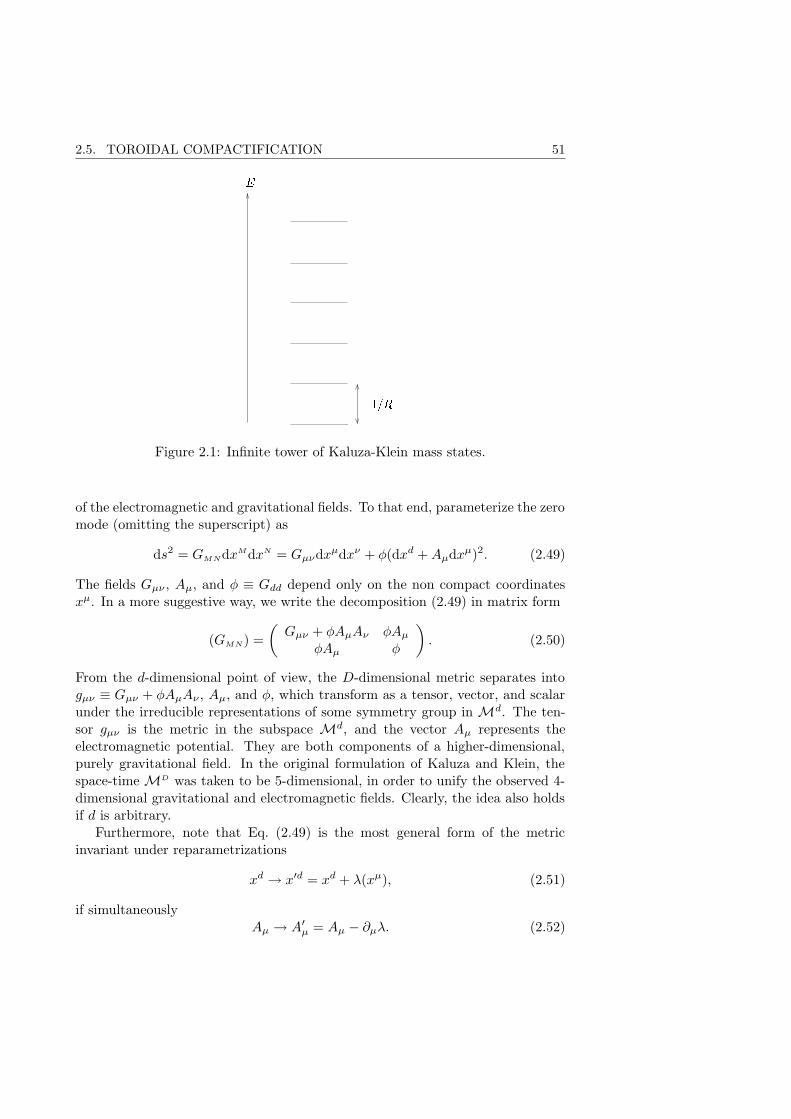
2.5. TOROIDAL COMPACTIFICATION 51
Figure 2.1: Infinite tower of Kaluza-Klein mass states.
of the electromagnetic and gravitational fields. To that end, parameterize the zeromode (omitting the superscript) as
ds2 = GMNdxMdxN = Gµνdxµdxν + φ(dxd +Aµdxµ)2. (2.49)
The fields Gµν , Aµ, and φ ≡ Gdd depend only on the non compact coordinatesxµ. In a more suggestive way, we write the decomposition (2.49) in matrix form
(GMN) =
(Gµν + φAµAν φAµ
φAµ φ
). (2.50)
From the d-dimensional point of view, the D-dimensional metric separates intogµν ≡ Gµν + φAµAν , Aµ, and φ, which transform as a tensor, vector, and scalarunder the irreducible representations of some symmetry group in Md. The ten-sor gµν is the metric in the subspace Md, and the vector Aµ represents theelectromagnetic potential. They are both components of a higher-dimensional,purely gravitational field. In the original formulation of Kaluza and Klein, thespace-time MD was taken to be 5-dimensional, in order to unify the observed 4-dimensional gravitational and electromagnetic fields. Clearly, the idea also holdsif d is arbitrary.
Furthermore, note that Eq. (2.49) is the most general form of the metricinvariant under reparametrizations
xd → x′d = xd + λ(xµ), (2.51)
if simultaneouslyAµ → A′
µ = Aµ − ∂µλ. (2.52)
52 CHAPTER 2. EXTRA-DIMENSIONS
This is easily seen by applying the transformation laws:
dx′d +A′µdxµ = dxd + dλ+Aµdxµ − (∂µλ)dxµ = dxd +Aµdxµ. (2.53)
Notice that the scalar λ does not depend on xd, and thus dλ = (∂µλ)dxµ. Hence,remarkably, the d-dimensional gauge transformations (2.52) arise from higher-dimensional coordinate transformations. The conserved quantity associated withinvariance under (2.51) is the momentum along S1.
Unfortunately, the theory of Kaluza and Klein does not work in practice,because the field φ acts as a Brans-Dicke scalar, which modifies 4-dimensionalgravity in a non acceptable way. Nevertheless, their idea shows the virtues (anddangers) of a higher-dimensional approach, and it is the prototype of other uni-fying theories.
Nowadays, string theory is the most promising candidate of such a theory.We have seen in Sec. 2.3, that it predicts a 10-dimensional space-time. To makecontact with the observed world, the first step is to take the low energy limit, inwhich case the action of type IIB string theory is given by Eq. (2.1). The secondstep is to compactify six spatial dimensions. In the next paragraph, we show howthis affects the low energy action.
2.5.2 Dimensional reduction of the action
Consider the action (2.1) and, for simplicity, keep only the Riemann scalar andthe dilaton kinetic term. One then obtains the ‘dilaton-gravity action’
SD =1
2κ2D
∫dDx√−G e−2Φ (R+ 4(∇MΦ)(∇MΦ)) . (2.54)
Commonly, this action is used for D = 10, D = 5, and D = 4, passing from oneto the other by a dimensional reduction. To see how this works in detail, assumethat the xd-direction is compact (where D = d + 1). The dependence on xd canthen be Fourier transformed according to Eq. (2.45), and only the zero modes arekept, for instance, Φ = Φ(xµ), and the index on the derivative M is replaced byµ.
The Ricci scalar for the metric (2.49) can be decomposed as
R = Rd − 2e−b(∇µ∇µeb)− 1
4e2bFµνF
µν , (2.55)
where we have defined e2b ≡ Gdd, Fµν ≡ ∂µAν − ∂νAµ, and R is constructedfrom the full D-dimensional metric GMN , whereas Rd from Gµν (but not fromgµν ≡ Gµν + e2bAµAν). Inserting this into the action (2.54) yields
Sd =1
2κ2D
∫dxd
∫ddx
√−Gd ebe−2Φ
(Rd − 2e−b(∇µ∇µeb)
+ 4(∇µΦ)(∇µΦ)− 1
4e2bFµνF
µν),
(2.56)
2.5. TOROIDAL COMPACTIFICATION 53
where Gd denotes the determinant of Gµν . The integral over xd simply gives 2πR,and the factor eb, coming from the volume element of the compact direction, canbe absorbed by defining a d-dimensional dilaton Φd(x
µ) = Φ(xµ)− b(xµ)/2. Thisleads to
Sd =πR
κ2D
∫ddx
√−Gd e−2Φd
(Rd − (∇µb)(∇µb)
+ 4(∇µΦd)(∇µΦd)−1
4e2bFµνF
µν).
(2.57)
We have assumed that the equation of motion for the modulus field b is ∇µ∇µb =0, such that the corresponding term from the derivative is zero. The dimensionalreduction leads to kinetic terms for the fields b(xµ),Φd(x
µ), Aµ(xµ). In Sec. 2.2,we have seen that the wrong sign and prefactor of the dilaton kinetic term is dueto the fact that the action is written in the string frame instead of the physicalEinstein frame. On the other hand, the dimensional reduction itself does not leadto potential terms, and so the fields b(xµ),Φd(x
µ), Aµ(xµ) are massless.
In addition to toroidal compactifications, there exist also compactifications onCalabi-Yau manifolds. These manifolds have a more complex structure and leadto phenomenologically more realistic particle physics theories.
2.5.3 Horava-Witten compactification
For brane world cosmologies, a compactification scheme due to Horava and Wit-ten [77] is particularly interesting, and we shall briefly discuss it here. In thisscenario, one starts from 11-dimensional M theory, which contains the five 10-dimensional superstring theories in different corners of its moduli space. Assumethat the eleventh dimension is curled up to a circle S1, and that this circle has amirror symmetry Z2. The coset space S1/Z2 is called an orbifold15. If θ denotesthe coordinate on S1, there are two fixed points at θ = 0 and θ = π, at which thecoset space becomes singular. This can be avoided by placing a 10-dimensionalhypersurface at each singular point. Since those hypersurfaces with nine spatialand one time direction have particular properties, e.g. a tension, they correspondto 9-branes16. As a condition for stability, the sum of the two tensions mustbe zero. In other words, there is a positive and a negative tension brane. In acosmological framework, the sign of the tension is important, for it determineswhether gravity on a brane is attractive or repulsive. Moreover, the positivity ofthe tension is a condition for local stability.
So far, space-time has the structure R10 × S1. Now, on each 9-brane, one can
compactify six spatial dimensions to end up with two parallel 3-branes residingat the orbifold fixed points. The resulting space-time is effectively 5-dimensional,and the S1 plays the role of the fifth dimension.
15In general, an orbifold is the coset space M/H, where H is a group of discrete symmetries ofthe manifold M.
16The meaning and properties of p-branes are introduced in Chap. 3
54 CHAPTER 2. EXTRA-DIMENSIONS
This setup is very common in brane cosmology, where one of the two 3-branesis identified with our universe. Particularly interesting is that, before compacti-fication, each of the 9-branes carries an E8 gauge group of the heterotic string.After compactification, the E8 is broken to SU(3)×SU(2)×U(1), and hence thestandard model of particle physics can be accommodated on a brane.
2.6 The modifications of Newton’s law
Gravity propagates in all dimensions, because it is the dynamics of space-timeitself. In particular, it is sensitive to the presence of extra-dimensions. This isnot the case for the electromagnetic, the strong, and the weak forces. In stringtheory, the graviton corresponds to an excitation of a closed string, and as suchit is free to propagate everywhere. Gauge particles, instead, correspond to openstring ends, which are confined to lower-dimensional hypersurfaces (see Sec. 3.4).
In this section, we study the modifications of Newton’s law in the presenceof n extra-dimensions. In principle, this allows to detect extra-dimensions in alaboratory experiment.
2.6.1 Newton’s law in d non compact spatial dimensions
First, let us generalize Newton’s law to a number d = 3 + n non compact spatialdimensions. Given a mass M , we want to find the force F exerted on a test massµ a distance r away. In a d-dimensional space, the source M is enclosed by a(d− 1) = (2 + n)-dimensional sphere S2+n. Gauss’ theorem is
∫
S2+n
F · dS =
∫
B3+n
(∇ · F) dV, (2.58)
where B3+n is a 3 + n-dimensional ball, whose surface is S2+n. Since F is per-pendicular onto every surface element dS, the left hand side gives
F
∫
S2+n
dS = Fr2+n|S2+n|, (2.59)
where the surface area of the (2 + n)-sphere is given by |S2+n| = 2π(3+n)/2
Γ((3+n)/2) . To
evaluate the right hand side of Eq. (2.58), we use the gravitational field equation17
∇ · g = |S2+n|GDρ, (2.60)
where GD denotes Newton’s constant in D = d+ 1-dimensional space-time. Thenormalization is chosen to cancel the surface area on the left hand side. Recallthat for n = 0, this factor gives 4π. Substituting F = µg, we get
µ
∫
B3+n
(∇ · g) dV = µ|S2+n|GD
∫
B3+n
ρ dV = µ|S2+n|GDM. (2.61)
17The second field equation would be ∇∧ g = 0, i.e. the gravitational field has no curl.
2.6. THE MODIFICATIONS OF NEWTON’S LAW 55
Equating Eqs. (2.59) and (2.61) gives
F = GD
µM
r2+n. (2.62)
This is Newton’s law if there are n non compact extra-dimensions. The factor1/rn reflects the dilution of field lines into the additional space. Notice alsothe appearance of the D-dimensional instead of the 4-dimensional gravitationalconstant.
2.6.2 Newton’s law with n compact extra-dimensions
Now assume that there are n compact extra-dimensions, each of size L, in additionto the usual three non compact directions. This situation can be reproduced bya setup with 3 + n non compact dimensions and mirror masses M placed at thepoints kL, k ∈ Z, along each of the extra-dimensions. Again, we want to find theforce F on a test mass µ at a distance r from the origin. If r ¿ L, the influence ofthe mirror masses is negligible, and the result is the same as for a single source Mand d = 3+n non compact spatial dimensions, derived in the previous paragraph:
F = GD
µM
r2+nfor r ¿ L. (2.63)
In particular, this is true if r is a distance in our universe. This allows us to test,in principle, whether there exist extra-dimensions by measuring the force betweentwo test bodies in the laboratory. There is no need to access the extra-dimensionsas the lines of force do it for us.
At distances r À L, a test mass feels the influence of the mirror masses, butit cannot discern their discrete spacing. Let us take r to be a distance in ouruniverse, and discuss first the case n = 1. Then the mirror masses look likeline of uniform mass density M/L. For symmetry reasons, we enclose it with acylinder of length Lc and suitable end caps whose contribution will vanish in thelimit Lc → ∞, see Fig. 2.2. Again, we use Gauss’ law (2.58), where on the lefthand side the integration domain is now the surface of the cylinder ∂C = R×S2.Then
F
∫
∂C
dS = FLc(4πr2). (2.64)
For the right hand side of (2.58) one uses again the field equation (2.60) (withn = 1) as all dimensions are non compact
µ|S2+1|GD
∫
C
ρ dV = µ|S2+1|GD
(LcM
L
). (2.65)
Solving for F one finds
F =|S2+1|GD
4πL
µM
r2. (2.66)
The artificial cut-off Lc has dropped out. It is now straightforward to generalize
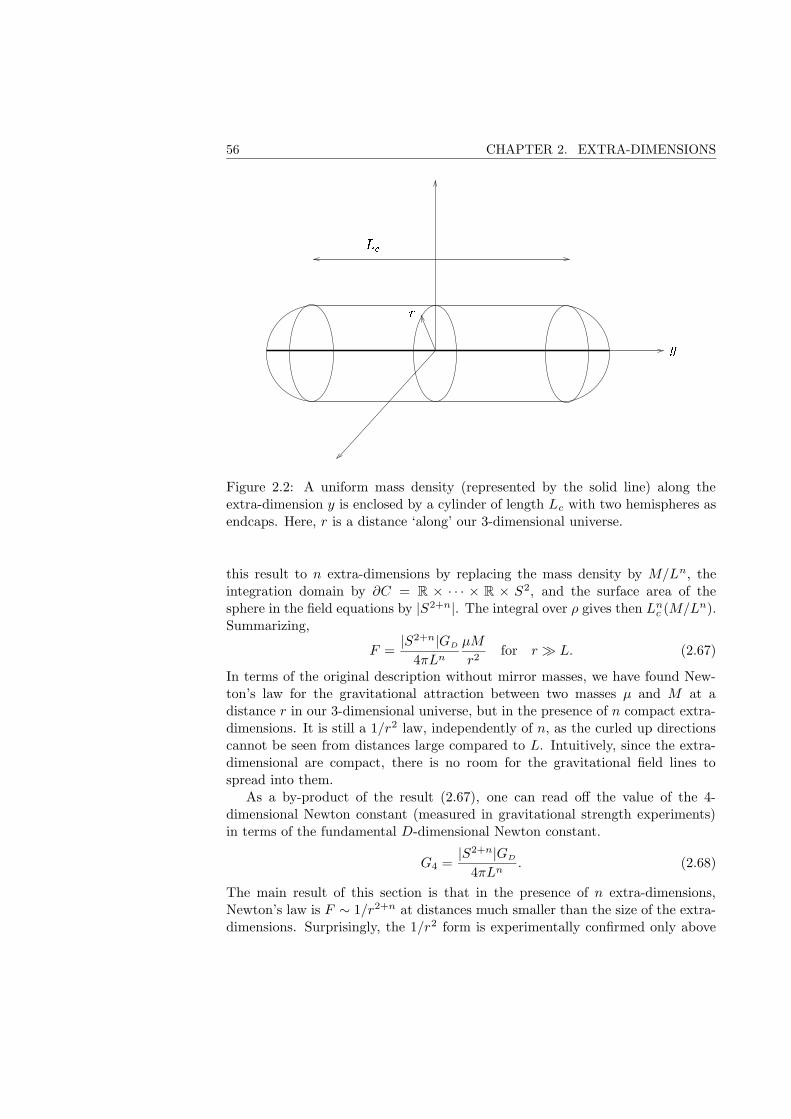
56 CHAPTER 2. EXTRA-DIMENSIONS
Figure 2.2: A uniform mass density (represented by the solid line) along theextra-dimension y is enclosed by a cylinder of length Lc with two hemispheres asendcaps. Here, r is a distance ‘along’ our 3-dimensional universe.
this result to n extra-dimensions by replacing the mass density by M/Ln, theintegration domain by ∂C = R × · · · × R × S2, and the surface area of thesphere in the field equations by |S2+n|. The integral over ρ gives then Ln
c (M/Ln).Summarizing,
F =|S2+n|GD
4πLn
µM
r2for r À L. (2.67)
In terms of the original description without mirror masses, we have found New-ton’s law for the gravitational attraction between two masses µ and M at adistance r in our 3-dimensional universe, but in the presence of n compact extra-dimensions. It is still a 1/r2 law, independently of n, as the curled up directionscannot be seen from distances large compared to L. Intuitively, since the extra-dimensional are compact, there is no room for the gravitational field lines tospread into them.
As a by-product of the result (2.67), one can read off the value of the 4-dimensional Newton constant (measured in gravitational strength experiments)in terms of the fundamental D-dimensional Newton constant.
G4 =|S2+n|GD
4πLn. (2.68)
The main result of this section is that in the presence of n extra-dimensions,Newton’s law is F ∼ 1/r2+n at distances much smaller than the size of the extra-dimensions. Surprisingly, the 1/r2 form is experimentally confirmed only above
2.7. THE HIERARCHY PROBLEM 57
r ' 20µm [42]. From the experimenter’s point of view, this is due to the weaknessof gravity compared to the Coulomb force. It is extremely difficult to eliminatedisturbing influences such as small electric charges on the probes to obtain a clearsignal. The lower limit on the validity of Newton’s law is at the same time theupper limit on the size of L. Extra-dimensions are thus not excluded as long astheir size is smaller than 20µm.
Whereas gravity is sensitive to extra-dimensions, gauge interactions are not.This is because gauge particles are confined to our universe (see Sec. 3.4). For thatreason, extra-dimensions have not been detected in collider experiments, whichtest gauge interactions down to 1/(200 GeV).
2.7 The hierarchy problem
The Einstein-Hilbert action of general relativity is
S4 =1
16πG4
∫d4x√−g R(g) ≡ M2
4
2
∫d4x√−g R(g). (2.69)
Here, we are interested only in the prefactor which has dimensions of a masssquared in order to make the action dimensionless. This mass is called the Planckmass18 and is defined via the only free parameter in general relativity, Newton’sconstant
M4 ≡1√
8πG4
= 2.4× 10¹⁸GeV. (2.70)
This relation defines the ‘energy scale of gravity’. For gauge interactions, instead,an important scale is the ‘electroweak scale’ defined as the energy at which therunning coupling constants αEM and αW are of the same size, and the electro-magnetic and the weak force are unified to a SU(2) × U(1) gauge theory. Thenumerical value of the electroweak scale is roughly 1 TeV.
Why do these two scales differ by a factor 1015? Another way of formulatingthis ‘hierarchy problem’ is: why is gravity so much weaker than the the otherfundamental forces? If one attempts to unify gravity and gauge interactions,their coupling constants should be at least of the same order, otherwise one hasto specify a mechanism which explains this huge difference. In the following, weare discussing an idea to solve the hierarchy problem.
2.7.1 Fundamental and effective Planck mass
In Sec. 2.6 we have seen that the 4-dimensional Newton constant is related tothe D-dimensional gravitational constant by Eq. (2.68). Here, we derive thisrelation in an alternative way, and in terms of mass scales rather than gravitational
18More precisely, Eq. (2.70) defines the reduced Planck mass in which numerical factors of orderone and factors of π are absorbed.
58 CHAPTER 2. EXTRA-DIMENSIONS
constants. The action of a D-dimensional theory (supergravity, low energy stringtheory) is
SD =1
2κ2D
∫dDx√−G (R+ · · · ) ≡ MD−2
D
2
∫dDx√−G (R+ · · · ), (2.71)
where we have defined a D-dimensional Planck mass MD. The power on MD
is D− 2 = 2 + n in order to make the action dimensionless. Note that, as we areinterested in physical masses, we have placed ourselves in the Einstein frame.
Assuming that the xd direction is a circle, and carrying out a dimensionalreduction as described in Sec. 2.5, one finds
SD =MD−2
D
2
∫dxd
√Gdd
︸ ︷︷ ︸
=MD−3
D−1
2
∫dD−1x
√−Gd (Rd + · · · ). (2.72)
Therefore, the (D − 1)-dimensional Planck mass is given by19
MD−3D−1 = MD−2
D V, (2.73)
where V the volume of the compactified dimension. To arrive at an effectivetheory in four space-time dimensions, this procedure is repeated for the remain-ing n − 1 extra-dimensions, and the overall coefficient is identified with the 4-dimensional Planck mass
M24 = MD−2
D Vn = M2+nD Vn, (2.74)
where Vn denotes the volume of the n-dimensional compact space. Note that thisformula holds not only for toroidal, but all kinds of compactifications in whichspace-time has a product structure MD = M1 ×M2, where our universe is a(sub)space ofM1 and the space of extra-dimensions is M2.
2.7.2 The idea of ‘large’ extra-dimensions
A solution to the hierarchy problem based on the relation (2.74) was suggestedby the authors of Refs. [12, 13]. Their idea is that the 4-dimensional Planck massis only a derived scale, whereas the relevant scale is the D-dimensional Planckmass which could be around 1 TeV.
Let us write Vn = Ln where L is the size of an extra-dimension. SettingMD ' 1 TeV, Eq. (2.74) gives
L ' 10(30/n)−17cm. (2.75)
19Note that in the Einstein frame the factor√
Gdd cannot be absorbed in a redefinition of thedilaton.
2.7. THE HIERARCHY PROBLEM 59
For n = 1, L ' 1013 cm, which is excluded because in this case the modifiedNewton law (2.63) would apply up to solar-system distances. Obviously this isnot the case. For n = 2, however, L ' 1 mm which is only marginally excluded byexperiments (see the end of Sec. 2.6). Therefore, a scenario with two ‘large’ extra-dimensions could possibly solve the hierarchy problem. To satisfy simultaneouslyother experimental constraints, coming for example from the production of mass-less higher-dimensional gravitons at the TeV scale, at least three extra-dimensionsare actually needed. One also has to keep in mind that this result relies on the as-sumptions that the fundamental Planck mass really is around 1 TeV, and that thespace-time does have a product structure. In Chap. 6 we present an alternativeattempt to solve the hierarchy problem due to Randall and Sundrum.

Chapter 3
Branes
62 CHAPTER 3. BRANES
3.1 Extended objects
In general relativity the elementary objects are point-like particles moving on afour-dimensional manifold with a metric and a certain symmetry group. Thoseparticles have to be test particles in the sense that their masses are negligible,otherwise the metric along the trajectory becomes singular. In quantum fieldtheory, the elementary objects are approximated by point-like particles, althoughtheir wave function is spread in space.
The first example of classical elementary extended objects were topologicaldefects formed during phase transition, e.g. cosmic strings and domain walls. Ina 4-dimensional space-time domains walls are the biggest (apart from space-filling)objects that can exist. A D-dimensional space-time, however, can be populatedby extended objects, having up to p = D − 1 spatial dimensions. A generaldefinition of such p-branes is [37]: a p-brane is a dynamical system defined interms of fields with support confined to a (p+1)-dimensional world-sheet surfacein a background space-time manifold of dimension D ≥ p + 1. The category p-brane includes particles (zero-branes), strings (1-branes), membranes (2-branes),and so on, up to space filling branes (p + 1 = D), which are continuous media,and where the confinement condition is redundant. The latter are not of primaryinterest for us. In this context, our 4-dimensional universe is conceived as a3-brane, to which gauge fields and fermionic fields are confined. String theoryprovides a natural explanation for why matter can be trapped on a hypersurface.In addition, there exist also more phenomenological approaches [133].
We begin this chapter with some geometrical preliminaries, which are essentialto describe p-branes. Section 3.3 explaines how p-branes emerge as solitonicsolutions of supergravity, and how anti-de Sitter space arises in this context. InSec. 3.4 we introduce Dp-branes from a string-theoretical point of view.
3.2 Differential geometrical preliminaries
This section serves as an introduction to a few geometrical concepts which areuseful in brane cosmology. We try to give a self-consistent overview, mainlyfollowing Refs. [37] and [150]. The theory is fully covariant and applies to classicalrelativistic branes. These include supergravity p-branes, string theory D-branesin the low energy limit, as well as topological defects and brane gases. It alsocovers a wide range of physical systems such as metal plates in an electromagneticfield or soap bubbles. In all cases, it is assumed that the branes are infinitely thin,which is a good approximation if their curvature radius is much larger than theiractual thickness.
In the first part, we define the first and second fundamental form for an ar-bitrary number of co-dimensions. Afterwards, we restrict ourselves to one co-dimension and discuss the equations of Gauss, Codazzi, and Mainardi, as wellas the junction conditions and their relevance for brane cosmology. At the same
3.2. DIFFERENTIAL GEOMETRICAL PRELIMINARIES 63
time, this section is a good place to fix our notations and conventions and a fewdelicate signs.
3.2.1 Embedding of branes
Consider a D-dimensional Lorentzian manifoldMD with a non degenerate metricG. Locally, it is always possible to choose coordinates xM , M = 0, · · · , D − 1.The corresponding metric components are denoted GMN . OnMD imagine a num-ber of intersecting or non intersecting hypersurfaces Ni, i = 1, · · · , n, which aresubmanifolds of MD. The number of co-dimensions of a submanifold is equal todim(MD)− dim(Ni). In cosmological applications those submanifolds or hyper-surfaces are world-sheets of branes, and therefore the number of co-dimensions isequal to the number of spatial extra-dimensions.
For practical purposes, it is useful to introduce locally a system of internalcoordinates σµ on Ni. An immersion1 of Ni inMD is given by the mapping
XM :Ni −→MD
σµ 7−→ xM(3.1)
with, for example, x0 = σ0, · · · , xp = σp, xp+1 = 0, xd = 0, if Ni is a (p+1)-dimensional submanifold. Conversely, if xM is given, it is always possible tochoose locally internal coordinates σµ on Ni according to the prescription above,since there exist p + 1 coordinate diffeomorphisms σ → σ(σ), which leave theLagrangian invariant. Globally, this need not always be the case, for example ifthe branes are intersecting, or in a cluster of soap bubbles.
At each point q of Ni one can define the tangent space TqNi. A basis of TqNi
is given by the p+ 1 vectors ∂∂σ0 , · · · , ∂
∂σp . An arbitrary vector in TqNi has thencomponents
eM
µ =∂XM
∂σµ. (3.2)
Knowing eMµ one can explicitly construct the internal2 metric gµν on the brane
Ni via the pull-back
gµν = GMNeM
µ eN
ν . (3.3)
Suppose now that the action of the compound system of branes is the sum3
S = S1 + · · ·+ Sn, where
Si =
∫dp+1σ
√−gLi (3.4)
is the action of a single brane. The Lagrangian density Li depends only on fieldsliving on the i-th brane, which, however, may be induced by external fields. The
1An immersion is a locally injective mapping.2We shall use ‘internal’, ‘intrinsic’, and ‘induced’ metric as synonyms.3This is for example the case in the Randall-Sundrum model with n = 2. Notice also that for
this consideration we do not take into account possible bulk terms.
64 CHAPTER 3. BRANES
conserved Noether currents and the surface energy-momentum tensor of the i-thbrane are
jµ =∂Li
∂pµ, (3.5)
tµν = −2δLi
δgµν+ Lig
µν , (3.6)
for each canonical momentum pµ. The symbol δ denotes a variational (Eulerian)derivative. There are other internal quantities, for example the Riemann tensorconstructed from gµν , if the action includes curvature terms. For specific compu-tational purposes, it may be convenient to work with gµν , j
µ, and tµν . However,if there are more or intersecting branes, the choice of internal coordinates is awk-ward. In this case, it is more advantageous to work with D-dimensional tensorsof the background. One defines the D-dimensional energy momentum tensor bythe push-forward
TMN = tµνeM
µ eN
ν . (3.7)
This tensor is defined only at the location of the brane. In this way, all internaltensorial quantities can be lifted to become tensors of the full space-time MD.The calculations are then carried out with those background tensors. Furtheradvantages of this approach are the absence of delta functions, which otherwiseappear at the position of the branes, as well as conceptual simplicity. However ingeneral, which view is more favorable to adopt, depends on the specific problem.
3.2.2 The first fundamental form
To construct TMN according to Eq. (3.7), one must nevertheless specify internalcoordinates σµ and an embedding to obtain the basis vectors eM
µ . So in the end,using D-dimensional quantities would not be more economic or simple. Thereis an alternative way to find TMN , or in fact any D-dimensional tensor, withoutfalling back on the use of internal coordinates. Assume that Ni is a strictlytime-like or space-like hypersurface. Then, at any point q of Ni, it is possible todecompose the D-dimensional metric tensor into a part tangential and orthogonalto the surface element as
GMN = qMN +⊥MN . (3.8)
The tangential part qMN is called first fundamental form. It is a D-dimensionaltensor, but only defined on the hypersurface Ni. The action of the mixed tensorqM
N is to project any D-dimensional tensor at a point q ∈ Ni onto the tangentspace TqNi. Similarly, ⊥M
N is an orthogonal projector. They satisfy
qM
AqA
N = qM
N , ⊥MA⊥A
N = ⊥MN , qM
A⊥AN = 0. (3.9)
For example, one can define a D-dimensional covariant derivative, that differen-tiates along the hypersurface, by
qC
M∇C ≡ ||∇M . (3.10)
3.2. DIFFERENTIAL GEOMETRICAL PRELIMINARIES 65
Notice that ||∇M is not the covariant derivative associated with the internal metricgµν , but only a tangential projection of the D-dimensional connection. We shallmake extensive use of this in the next paragraph.
With the aid of qMN , the D-dimensional tensor TMN in Eq. (3.7) can beobtained without a detour on the induced metric simply by varying the Lagrangianwith respect to the bulk metric
TMN = −2δLi
δGMN
+ LiqMN . (3.11)
In the second term, we have written qMN instead of GMN , since TMN is equalto its own tangential part4. Calculations involving the energy-momentum tensoron the brane can now be carried out using this equivalent background quantity.Recall that the link with the original internal quantity is still given by Eq. (3.7).
An alternative definition of the first fundamental form is
qMN = gµνeM
µ eN
ν . (3.12)
This is seen by writing Eq. (3.8) as
GMN = qMN +⊥MN = gµνeM
µ eN
ν +⊥MN , (3.13)
i.e. the full metric on MD can be constructed by lifting the internal metric to aD-dimensional tensor, namely the metric along the submanifold Ni, and addingthe orthogonal complement. Here, also the difference between qM
N and eMµ be-
comes evident: eMµ promotes (pushes-forward) a tensor on Ni to a D-dimensional
tensor and vice versa. In contrast, qMN simply projects a D-dimensional tensors
to its own tangential part. A useful relation for calculations (see for exampleparagraph 3.2.5) is
qMN = GABqM
AqN
B, (3.14)
which simply states that the projection of the D-dimensional metric yields the(also D-dimensional) metric along Ni. In particular, qMN can be used to raiseand lower indices of D-dimensional tangential tensors.
3.2.3 The second fundamental form
At any point q of the p-dimensional submanifold Ni, one can define the secondfundamental form
KMNA = −qB
N qC
M∇CqA
B = −qB
N
||∇MqA
B, (3.15)
which is tangential to Ni in its first two indices and orthogonal in the last. Thesecond fundamental form is the generalization of the extrinsic curvature tensor toan arbitrary number of co-dimensions. From the Weingarten equation, it follows
4The indices of the first fundamental form are pulled up and down with GMN , as for any D-dimensional tensor.
66 CHAPTER 3. BRANES
that K[MN]A = 0, where the square bracket denotes antisymmetrization. By
contracting over the tangential indices, one obtains the extrinsic curvature vector
KA = KMM
A, (3.16)
which is purely orthogonal onto Ni, i.e. ||KB = qBAK
A is identically zero. Thespecification of KA provides an equation of motion for the hypersurface. Whenthere are no external forces, it takes the simple form KA = 0. If the hypersurfaceis subject to an external force F A, e.g. due to some gauge field in the bulk, theequation of motion is
TMNKMNA = ⊥FA. (3.17)
The surface energy-momentum tensor TMN is provided by Eq. (3.7) or (3.11), and⊥FA = ⊥A
BFB is the orthogonal projection of the external force. For instance,
for a Nambu-Goto string (see Ref. [158]), TMN = −ρ δM
N , and form TMNKM
NA =
⊥FA one finds
KMM
A= KA = −1
ρ⊥F
A
. (3.18)
In addition, there exists a formalism to treat perturbations on a hypersurface interms of the first and second fundamental forms, see e.g. Ref. [16]. We shall makeuse of this in the case of one co-dimension in the article in Chap. 5.
3.2.4 First and second fundamental form for one co-dimension
So far, everything we have said is true for a hypersurface with an arbitrary numberof co-dimensions. In brane cosmology, motivated by Horawa-Witten compactifi-cation (see paragraph 2.5.3), one identifies our universe with a 3-brane embeddedin a 5-dimensional bulk. We therefore make the identification, that this 3-branecorresponds to N1, and that the bulk isM5. Some models also require the pres-ence of a second brane N2 which is aligned paralled to N1. In the following,however, we focus on a single brane and drop the subscript 1 to avoid clutteringthe notation.
The unit normal nM ⊥ TqN at the point q ∈ N is defined by the orthogonalityand normalization conditions
GMNnMeN
µ = 0, µ = 0, · · · , p,GMNn
MnN = ±1.(3.19)
The plus sign applies for a space-like unit normal (time-like brane), and the minussign for time-like unit normal (space-like brane). Causality requires that thetrajectory of a brane in the bulk is time-like, and therefore we shall always assumethe unit normal to be space-like, if not otherwise indicated5. The orthogonalmetric tensor can now be simply expressed in terms of the unit normal
⊥MN = nMnN , (3.20)
5In the well-known 3 + 1 splitting in general relativity, the unit normal is time-like. Therefore,care must be taken, when comparing our expressions with those in general relativity textbooks.
3.2. DIFFERENTIAL GEOMETRICAL PRELIMINARIES 67
such that full space-time metric can be decomposed as
GMN = qMN + nMnN . (3.21)
Also the second fundamental form can now be defined in terms of the unit normal
KMN = −qB
NqC
M∇CnB = −qB
N
||∇MnB. (3.22)
Note that ∇CnB is in general not in the tangent space TqN , therefore it needs tobe projected onto TqN by the first fundamental form. The indices M and N are‘tangential’, whereas B and C stand for arbitrary directions. KMN is symmetricin M and N . In Gaussian normal coordinates6 one has nC∇CnB = 0, since theunit normal is tangential to a geodesic of M5, and Eq. (3.22) reduces to
KMN = −∇MnN . (3.23)
The second fundamental form is linked to the usual extrinsic curvature tensorkµν , which measures ‘extrinsically’ the curvature of a hypersurface via the tilt ofthe unit normal as it is transported along the hypersurface. The relation is
KMN = kµνeM
µ eN
ν . (3.24)
Like in Eq. (3.7), KMN is defined only on the hypersurface N . According to thespecific problem, it is more convenient to work with kµν or KMN . A definition ofkµν consistent with (3.22) is
kµν = −eN
µ eM
ν ∇MnN . (3.25)
Indeed,
KMN = kµνeM
µ eN
ν = kµνeN
µ eM
ν = −(eµ)B(eν)C∇CnB eN
µ eM
ν
= − (eµ)BeN
µ︸ ︷︷ ︸=qBN
(eν)CeM
ν︸ ︷︷ ︸=qCM
∇CnB. (3.26)
Alternatively, kµν can be defined via the Lie derivative of the five-dimensionalmetric in the direction of the unit normal
kµν = −1
2eM
µ eN
ν LnGMN , (3.27)
because by definition of the Lie derivative7
LnGMN = nAGMN,A +GANnA
,M +GMAnA
,N
= nAGMN,A + (nN,M −GAN,MnA) + (nM,N −GMA,Nn
A)
= nN,M + nM,N − 2nAΓANM
= ∇MnN +∇NnM ,
(3.28)
6Gaussian normal coordinates are defined in the following way: from each point p in the neigh-borhood of N , a geodesic in M5 is dropped onto N , such that it intersects N orthogonally at apoint q. p is then uniquely characterized by indicating the coordinates of q and a proper distancealong the geodesic.
7We adopt the common, but untidy, notation LnGMN , for what is acutally (LnG)MN
. Similarly,one writes ∇MnN instead of (∇Mn)
N.
68 CHAPTER 3. BRANES
where we have used the product rule and replaced metric derivatives by Christoffelsymbols. Since the Lie derivative is symmetric, the definition (3.27) is indeedequivalent to kµν = −eM
µ eNν∇MnN given in Eq. (3.25).
A third equivalent definition is the following [150]: the extrinsic curvature is asymmetric bilinear form K(., .) acting on the tangent space TqN , which satisfies
∇XY = ∇XY +K(X,Y )n. (3.29)
Here, X,Y ∈ TqN and n⊥TqN . The symbol ∇ denotes the connection with
respect to the metric G in M5, and ∇ the connection for the internal metric gon N , given by Eq. (3.3). By taking the scalar product with n on both sides,
(∇XY, n) = (∇XY, n)︸ ︷︷ ︸=0
+K(X,Y ) (n, n)︸ ︷︷ ︸=1
, (3.30)
one findsK(X,Y ) = (∇XY, n). (3.31)
We now use the Ricci identity XG(Y, Z) = (∇XY, Z) + (Y,∇XZ). The left handside is zero, for ∇ is a metric connection, i.e. ∇G = 0. Setting Z = n, one finds
K(X,Y ) = −(Y,∇Xn), (3.32)
which is equivalent to Eq. (3.23). Indeed, to write this equation in componentform, we choose a basis e0, e1, e2, e3, n of TqM5, and set X = eM , Y = eN (bothin the tangential space). Then
KMN = K(eM , eN) = −(eN ,∇eMn) = −(eN , (∇Mn
L)eL)
= −(∇MnL)(eN , eL) = −∇MnN .
(3.33)
3.2.5 The equations of Gauss, Codazzi and Mainardi
The Gauss equation (theorema egregium) provides a link between the intrinsicRiemann tensor on a submanifold with co-dimension one with the Riemann tensorof the embedding manifold. In brane cosmology, the Gauss equation is useful tofind the Riemann, Ricci, and Einstein tensors on a brane from those in the bulk.For concreteness, we consider as before a time-like 4-dimensional submanifoldN , embedded in a 5-dimensional Lorentzian manifold M5. The Gauss theorem(theorema egregium) is [150]:
Theorem 4. (Gauss)
(R(X,Y )Z,W ) = (R(X,Y )Z,W ) +K(X,Z)K(Y,W )−K(Y, Z)K(X,W ),(3.34)
where (R(X,Y )Z,W ) denotes the Riemann tensor of M5, constructed from themetric G, and R(X,Y )Z,W ) is the Riemann tensor of N , constructed from ggiven by the pull-back (3.3). All vector fields are tangential to the submanifold,
3.2. DIFFERENTIAL GEOMETRICAL PRELIMINARIES 69
i.e. X,Y, Z,W ∈ TqN .
The components of the Gauss equation are obtained by setting X = eC, Y =eD, Z = eB,W = eA. Hence
(R(eC, eD)eB, eA) = (R(eC, eD)eB, eA) +K(eC, eB)K(eD, eA)
−K(eD, eB)K(eC, eA)(3.35)
or, equivalently,
RMNRSqM
AqN
BqR
CqS
D = RABCD +KCBKDA −KDBKCA. (3.36)
Notice that we have used bulk indices M = 0, · · · , 4 according to the formalismintroduced before. Since RABCD is an internal brane quantity, it is clear thatits indices actually run only from 0 to 3. The bulk Riemann tensor is evaluatedat the position of the brane and tangentially projected8 by qM
AqN
BqR
CqS
D. Onthe other hand, the extrinsic curvature is by definition located on the brane andtangentially projected onto it.
A complementary equation is that of Codazzi and Mainardi [150]:
Theorem 5.
(R(X,Y )Z, n) = (∇XK)(Y, Z)− (∇YK)(X,Z), (3.37)
where X,Y, Z ∈ TqN and n⊥TqN .
In component language, with n = nAeA, it reads
nA(R(eC, eD)eB, eA) = ∇CKDB − ∇DKCB (3.38)
or, equivalently,
nARANRSqN
BqR
CqS
D = ∇CKDB − ∇DKCB. (3.39)
Here, only the last three indices of RANRS are projected onto the brane. Uponcontraction with GBD, a term qN
BqS
DGBD = qNS appears on the left hand side,
which is the 5-dimensional metric along N , and therefore can be used to contractover the second and fourth index of the Riemann tensor. One easily finds
RABnAqB
C = ∇CK − ∇DKCD. (3.40)
We have used the notation K ≡ KDD for the trace.
The equations of Gauss, Codazzi, and Mainardi are useful to split the 5-dimensional Einstein tensor,
GAB = RAB −1
2GABR, (3.41)
8Alternatively, we could have written ||RABCD for the left hand side.
70 CHAPTER 3. BRANES
into ‘mixed’, ‘orthogonal’, and ‘parallel’ components with respect to the time-like hypersurface N (see Ref.[19]). The mixed component corresponds directly toEq. (3.40), as the second term in Eq. (3.41) does not contribute upon contractionwith qB
C. Thus
GABnAqB
C = ∇CK − ∇DKCD. (3.42)
Similarly, the orthogonal component is
GABnAnB = −1
2R+
1
2
(K2 −KABK
AB), (3.43)
where R denotes the Riemann scalar constructed from the internal metric gµν .Finally, the parallel component is
GABqA
CqB
D = GCD −KKCD + nE∇EKCD + ∇CaD + 2n(CKD)EaE − aCaD
+(1
2K2 +
1
2KABK
AB − nA∇AK −∇BaB
)qCD,
(3.44)where GCD is the Einstein tensor constructed from the internal metric, aB =nC∇Cn
B is the ‘acceleration field’, and the round brackets denote symmetriza-tion with weight one half. Notice also the difference between the two covariantderivatives that appear in the above formula: ∇ associated with the metric GMN
and ∇ associated with gµν .
3.2.6 Junction conditions
So far, we have considered N to be an empty hypersurface. In a cosmologicalcontext, however, it corresponds to a brane with a certain energy density dueto matter and radiation. The energy content has an effect on the bulk space-time, and therefore the geometry on both sides must be matched in a proper way.The problem is somewhat subtle, because the smoothness of the bulk metric isinfluenced not only by the presence of the brane, but also by the particular choiceof coordinates to describe the bulk9. An example is the treatment of thin shells inordinary 4-dimensional general relativity. In Ref. [82] a formalism was developed,making no reference to coordinate systems, in order to study boundary surfaces orshock waves, where the density jumps, as well as surface layers, where it becomesinfinite. Earlier work on the subject has been done by Refs. [99], [141], and [45].The same formalism is equally suited for brane cosmology.
We want to know about the local geometry due to some matter distribution.Therefore we start with the 5-dimensional Einstein equations written in the form
RAB = κ25
(TAB −
1
3GABT
), (3.45)
9In Newtonian theory, the solution of a matching problem is straightforward: there is no problemin setting up a well-defined coordinate system, and one simply has to impose continuity and jumpconditions for the Newtonian potential and its first derivative across the hypersurface.
3.2. DIFFERENTIAL GEOMETRICAL PRELIMINARIES 71
where T ≡ TAA denotes the trace of the 5-dimensional energy-momentum tensor.
The unusual factor 1/3 arises because GABGAB = 5 rather than 4. Assume that
the brane has a finite thickness ε, and let N< and N> denote the two boundariesof N . A Gaussian normal coordinate y is defined such that y = 0 on N< andy = ε on N>. In Gaussian normal coordinates, the 5-dimensional Ricci tensor,projected onto the brane, can be written as [82]
RCDqC
AqD
B =∂KAB
∂y+ RAB −KKAB + 2KA
CKCB. (3.46)
This form of the Ricci tensor is inserted into the Einstein equations (3.45), andboth sides are integrated from N< to N>,
∫ ε
0
dy∂KAB
∂y+
∫ ε
0
dy(RAB −KKAB + 2KA
CKCB
)
= κ25
∫ ε
0
dy(TCDq
C
AqD
B −1
3GCDq
C
AqD
B︸ ︷︷ ︸=qAB
T).
(3.47)
Notice that, on the left hand side, all tensors are by definition tangential, whereason the right hand side the bulk energy-momentum tensor and the bulk metric haveto be projected onto each hypersurface in the integration domain. It is reasonableto expect that the second term on the left hand side is bounded between N < andN>, and therefore the integral vanishes in the limit ε→ 0.
We define the surface energy-momentum tensor of N by
SAB ≡ limε→0
∫ ε
0
dy TCDqC
AqD
B, (3.48)
where S = SABqAB denotes the trace. As a first junction condition, we assume
that the first fundamental form is continuous across N , i.e.
q>AB = q<
AB. (3.49)
In the limit of an infinitely thin brane, Eq. (3.47) then becomes
K>AB −K<
AB = κ25
(SAB −
1
3qABS
). (3.50)
In the literature, this is known as Israel’s junction condition10. The relations (3.49)and (3.50) guarantee the consistent matching of the bulk geometry across thebrane. In brane cosmology, motivated by the Horava-Witten compactificaton,one often works with a Z2-symmetric bulk, i.e. with a symmetry under y → −y.Then, K<
AB = −K>AB ≡ −KAB, and Eq. (3.50) becomes11
KAB =κ2
5
2
(SAB −
1
3qABS
), (3.51)
10Often they are written in terms of internal brane quantities, namely k>µν − k<
µν =
κ25
(Sµν − 1
3gµνS
), where Sµ
ν = diag(−ρ, P, P, P ), for example11The choice of the ‘right’ side of the brane as representative for the whole bulk can be subtle. See
the discussion in the article ‘On CMB anisotropies from vector perturbation in the bulk’.
72 CHAPTER 3. BRANES
i.e. the extrinsic curvature of the brane is completely determined by its mattercontent.
The power of this approach lies in the fact that it makes no reference to aparticular coordinate system, and that no knowledge is needed about the globalstructure of the manifold M5. The basic formalism is valid for time-like (asassumed here) and space-like hypersurfaces, but not for surfaces that are null,since then the concept of extrinsic curvature breaks down.
In this section, we have introduced various tensors to describe the geometry ofhypersurfaces, both from the full space-time point of view (qAB,KAB), and froman intrinsic point of view (gµν , kµν). We have shown how they are related to eachother, and how they can be used for practical calculations. Now, our aim is tomotivate the existence of such hypersurfaces by introducing p-branes, which arephysical objects arising in supergravity and string theory.
3.3 Branes from supergravity
3.3.1 The black p-brane geometry
Originally, p-branes were found as classical solutions to supergravity. Since 11-dimensional supergravity, compactified on a circle, is equivalent to the low energylimit of 10-dimensional type IIB string theory, we can start from the equationsof motion (2.7). We are looking for solutions that correspond to a p-dimensionalsource of charge Qp under the 4-form potential C4. The metric is required to havep-dimensional Euclidean symmetry and, for simplicity, spherical symmetry in theremaining 10− p dimensions. The spherical part, including time, has Lorentziansignature. In the string frame, the solution for the metric is [2]
ds210 = − f+(ρ)√f−(ρ)
dt2 +√f−(ρ)
p∑
i=1
dxidxi +f−(ρ)%
f+(ρ)dρ2 +ρ2f−(ρ)ςdΩ2
8−p, (3.52)
where ρ is the radial coordinate of the spherical part, xi are the spatial coordinatesalong the source, and dΩ2
8−p is the volume element of an 8−p sphere. Furthermore,we have defined
f±(ρ) = 1−(r±ρ
)7−p
, % = −1
2− 5− p
7− p, ς =1
2− 5− p
7− p. (3.53)
The solution for the dilaton field is
e−2Φ = g−2s f−(ρ)−
p−32 . (3.54)
Since f−(ρ) = 1 in the limit ρ → ∞, gs represents the asymptotic value of thestring coupling constant. For p = 3, the dilaton is constant.
Eq. (3.52) is called black p-brane solution, in analogy with the charged black-hole or Reissner-Nordstrom geometry. In particular, it has an inner and outer
3.3. BRANES FROM SUPERGRAVITY 73
horizon, r− and r+. When r+ > r−, the singularity is always shielded by thehorizon, and the p-brane can be regarded as a black-hole. In analogy with theReissner-Nordstrom case, this corresponds to the mass (density) of the sourcebeing larger than its charge (density), Mp > Qp.
In a string theoretical context, the source is formed by a stack of N Dp-branes on top of each other. The charge of a Dp-brane is equal to its tension τp,given in Eq. (3.73), such that Qp = Nτp. When r+ < r−, there is a time-likenaked singularity, which corresponds to the unphysical regime Mp < Qp in theReissner-Nordstrom case. Finally, if r− = r+, the lower bound on the mass issaturated, Mp = Qp. Such a solution is referred to as extremal p-brane, and itcorresponds to a ground state. For p 6= 3, the horizon and the singularity coincide,and the supergravity description for an extremal p-brane breaks down close tothe horizion. Then, one has has to resort to the full string theory description.For p = 3, however, the surface ρ = r− = r+ corresponds to a regular horizon,and it is this case that is particularly interesting for cosmology, if our universe isidentified with a 3-brane moving in the background of a black 3-brane solution.
To discuss extremal and non extremal solutions with r+ ≥ r−, we introduce aparameter rH measuring the departure from extremality,
r7−pH = r7−p
+ − r7−p− , (3.55)
and a new radial coordinate r,
r7−p = ρ7−p − r7−p− , (3.56)
which is suited to describe the region outside the inner horizon. Note that thep-brane source is located at ρ = 0, whereas r = 0 denotes the location of theinner horizon. We also define
Hp(r) = 1 +(r−r
)7−p
, Fp(r) = 1−(rH
r
)7−p
, (3.57)
where Hp is a harmonic function. Then
f− =1
Hp, f+ =
Fp
Hp. (3.58)
Inserting Eqs. (3.58) into the solution (3.52), and using that r7−p+r7−p− = Hp r
7−p
and dρ = r6−p
ρ6−p dr, the black p-brane geometry becomes
ds210 = H−1/2p
(−Fp(r)dt
2 +
p∑
i=1
dxidxi
)+H1/2
p
(dr2
Fp(r)+ r2dΩ2
8−p
). (3.59)
The metric (3.59) is completely equivalent to the original metric (3.52) in theregion outside the inner horizon. In the extremal limit, rH = 0 and Fp = 1, andthe Euclidean symmetry is enhanced to Poincare symmetry. Eq. (3.59) describes
74 CHAPTER 3. BRANES
the geometry induced by a p-dimensional source of mass Mp and charge Qp.These two parameters can be expressed in terms of r− and r+, and are thereforecontained in the function Hp(r) and Fp(r). For our purpose, they are not relevant,as we will be merely interested in a particular limit of the metric (3.59), namely ananti-de Sitter-Schwarzschild space-time (AdS5-S) which we are going to derive inthe next paragraph. Nevertheless, we find it instructive to see how the parametersof AdS5-S are linked to the fundamental supergravity solution.
Notice that p-branes are solitons of supergravity. When making the analogywith topological defects, a 0-brane corresponds to a monopole, a 1-branes to acosmic string, and a 2-brane to a domain wall. The peculiar case p = −1 is aninstanton. On the other hand, there is a close correspondence to string theory D-branes. We will comment on this and on the validity of the supergravity solutionin Sec. 3.4.
3.3.2 Anti-de Sitter space-time
The curvature of the geometry (3.59) is set by the horizon r−, which in turn isdetermined by the mass and the charge of the p-brane source. It is interestingto consider the black p-brane solution in the limit r ¿ r−. Because r = 0 corre-sponds to the horizon itself, this limit means being near the horizon. Therefore,the limit r ¿ r− is commonly called the near horizon limit. Let us define thevariable L ≡ r− for future convenience, and set p = 3. This choice will be justifiedbelow. Essentially, the near horizon limit then corresponds to the approximation
H3(r) = 1 +
(L
r
)4
'(L
r
)4
. (3.60)
The metric (3.59) then takes the form
ds210 = − r2
L2
(1− r4H
r4
)dt2 +
r2
L2
3∑
i=1
dxidxi +dr2
r2
L2
(1− r4
H
r4
) + L2dΩ25
≡ −f(r)dt2 + g(r)δijdxidxi +
dr2
f(r)+ L2dΩ2
5.
(3.61)
Thus, the 10-dimensional space-time splits intoM5×S5, whereM5 is a manifoldwith anti-de Sitter-Schwarzschild (AdS5-S) geometry and S5 is a 5-sphere. M5 isa non compact space-time, labelled by coordinates t, x1, x2, x3, r, and contains a3-dimensional Euclidean subspace. The volume element of the 5-sphere is givenby
dΩ25 = dθ2
1 + sin2(θ1)dθ22 + sin2(θ2)
[dθ23 + sin2(θ3)
(dθ24 + sin2(θ4)dθ
25
)].
(3.62)Moreover, we have defined metric functions f(r) and g(r) for later convenience(see. Chap. 5). Here, the parameter rH , which classified before whether thesolution is extremal (rH = 0) or non extremal (rH > 0) plays the role of a
3.3. BRANES FROM SUPERGRAVITY 75
horizon. In fact, without knowing the supergravity origin, one could interpret thegeometry (3.61) as arising from a black-hole at r = 0.
Let us now consider the extremal limit rH = 0 of the metric (3.61). Then,M5 becomes pure 5-dimensional anti-de Sitter space-time (AdS5 ), and togetherwith the spherical part, this is called the AdS5×S5 geometry. The metric of theAdS5 part is
ds25 =r2
L2
(−dt2 + δijdx
idxj)
+L2
r2dr2. (3.63)
In summary, we have shown that AdS5 arises from the black 3-brane super-gravity solution by taking both the near horizon limit and the extremal limit. Theinner horizon r− has become the curvature radius L of AdS5 , since by definitionL = r−. Of course, anti-de Sitter space-time exists also on its own right as amaximally symmetric solution of Einstein’s equations with a negative cosmologi-cal constant (see Sec. 2.4).
In brane world cosmology, AdS5 is particularly important due to the general-ized Birkhoff theorem [26]. Most brane world models consider an AdS5 background,and our universe is identified with a 3-brane moving in it. The observed homo-geneity and isotropy can be accommodated by choosing an embedding in whichthe brane is parallel to the Minkowskian part of the metric (3.63). This alsoexplains why we have chosen p = 3 at the beginning.
We end this section by giving some alternative forms of the AdS5 metric (3.63)which are useful in various calculations. First, by defining a new radial coordinatez ≡ L2/r, the metric (3.63) can be cast into the form
ds25 =L2
z2
(−dt2 + δijdx
idxj + dz2). (3.64)
Alternatively, one may work with a radial coordinate % ≡ −L ln (r/L), suchthat r2/L2 = e−2%/L. In these coordinates the metric (3.63) reads
ds25 = e−2%/L(−dt2 + δijdx
idxj)
+ d%2, (3.65)
which is the form used in the so-called Randall-Sundrum model: a Minkowskimetric on a 3-brane is multiplied by an exponentially decreasing ‘warp’ factor.
Finally, AdS5 space-time can be understood as a hyperboloid embedded in a6-dimensional flat space with coordinates (x0, x1, x2, x3, x4, x5) and a metric
ds26 = −dx20 − dx2
5 + dx21 + dx2
2 + dx23 + dx2
4 (3.66)
subject to the constraint
−x20 − x2
5 + x21 + x2
2 + x23 + x2
4 = −const2. (3.67)
76 CHAPTER 3. BRANES
3.4 Branes from string theory
In string theory there exist objects called Dp-branes, which are hypersurfacesrepresenting the geometrical locus where open strings end. The letter ‘D’ refers toDirichlet boundary condition, and ‘p’ stands for the number of spatial dimensionsas we are familiar with from the previous section. Their existence was first claimedin Ref. [126]. In this section we follow however the more pedagogic treatmentof [124], [125], and [83].
3.4.1 T-duality for open strings
To see how D-branes come about, recall the mode expansion for the open string,Eq. (2.10). An open string supports oscillatory modes travelling from its left to itsright end, and vice versa. To make this evident, one rewrites the solution (2.10)as
XM(τ, σ) = xM +pM
p+τ + i
(α′
2
)1/2∑
n6=0
αMn
n
(e−πn(icτ+iσ)/s + e−πn(icτ−iσ)/s
).
(3.68)The first term in the oscillatory modes is due to left-, the second due to right-movers. By the Neumann boundary condition they are not independent, thereforethere is just one amplitude αM
n for both. Note that we have replaced the index iin Eq. (2.10) by M = 0, · · · , D − 1 because, after all, the expansion is valid forall directions. We proceed now similarly as in paragraph 2.3.3: by an analyticcontinuation to a Minkowskian world-sheet, one defines a real coordinate σ0 =icτ and a complex variable z = eσ0+iσ. The time τ can then be expressed asτ = ln(|z|2)/(2ic). This time we chose the length of the (open) string to be s = π.Hence the velocity defined below Eq. (2.9) becomes c = 1/(2α′p+). In terms ofthe complex variables z and its conjugate z, Eq. (3.68) reads
XM(z, z) = XM(z) +XM(z)
=
x
M
2+x′M
2− iα′pM ln(z) + i
(α′
2
)1/2∑
n 6=0
αMn
nz−n
+
x
M
2− x′M
2− iα′pM ln(z) + i
(α′
2
)1/2∑
n6=0
αMn
nz−n
.
(3.69)
This splitting is analogous to Eq. (2.21) and attributes a holomorphic functionto the left-movers and an anti-holomorphic function to the right-movers. Wehave added a coordinate x′M whose meaning will soon become obvious. Assumethat one direction, xd say, is a circle with radius R. One can reparameterize the
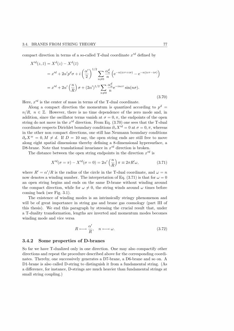
3.4. BRANES FROM STRING THEORY 77
compact direction in terms of a so-called T-dual coordinate x′d defined by
X ′d(z, z) = Xd(z)−Xd(z)
= x′d + 2α′pdσ + i
(α′
2
)1/2∑
n6=0
αdn
n
(e−n(icτ+iσ) − e−n(icτ−iσ)
)
= x′d + 2α′( nR
)σ + (2α′)1/2
∑
n6=0
αdn
ne−incτ sin(nσ).
(3.70)Here, x′d is the center of mass in terms of the T-dual coordinate.
Along a compact direction the momentum is quantized according to pd =n/R, n ∈ Z. However, there is no time dependence of the zero mode and, inaddition, since the oscillator terms vanish at σ = 0, π, the endpoints of the openstring do not move in the x′d direction. From Eq. (3.70) one sees that the T-dualcoordinate respects Dirichlet boundary conditions ∂τX
′d = 0 at σ = 0, π, whereasin the other non compact directions, one still has Neumann boundary conditions∂σX
M = 0,M 6= d. If D = 10 say, the open string ends are still free to movealong eight spatial dimensions thereby defining a 8-dimensional hypersurface, aD8-brane. Note that translational invariance in x′d direction is broken.
The distance between the open string endpoints in the direction x′d is
X ′d(σ = π)−X ′d(σ = 0) = 2α′( nR
)π ≡ 2πR′ω, (3.71)
where R′ = α′/R is the radius of the circle in the T-dual coordinate, and ω = nnow denotes a winding number. The interpretation of Eq. (3.71) is that for ω = 0an open string begins and ends on the same D-brane without winding aroundthe compact direction, while for ω 6= 0, the string winds around ω times beforecoming back (see Fig. 3.1).
The existence of winding modes is an intrinsically stringy phenomenon andwill be of great importance in string gas and brane gas cosmology (part III ofthis thesis). We end this paragraph by stressing the crucial result that, undera T-duality transformation, lengths are inverted and momentum modes becomeswinding mode and vice versa
R←→ α′
R, n←→ ω. (3.72)
3.4.2 Some properties of D-branes
So far we have T-dualized only in one direction. One may also compactify otherdirections and repeat the procedure described above for the corresponding coordi-nates. Thereby, one successively generates a D7-brane, a D6-brane and so on. AD1-brane is also called D-string to distinguish it from a fundamental string. (Asa difference, for instance, D-strings are much heavier than fundamental strings atsmall string coupling.)
78 CHAPTER 3. BRANES
0 R’2π
Figure 3.1: The horizontal axis corresponds to the T-dual coordinate x′d. Anopen string with winding number zero starts and ends on the same Dp-brane,whereas an open string with single winding can be represented by identifying thehyperplanes on the left and on the right. Note that those are not Dp-branes; theyjust symbolize the periodic identification.
Let us take a closer look at the action of T-duality. Along the brane, the openstring ends are subject to the Neumann boundary conditions. Upon T-dualizingin a tangential direction, an additional Dirichlet boundary condition arises, anda Dp-brane is turned into a D(p-1)-brane. Similarly, a T-duality in an orthogonaldirection turns a Dp-brane into a D(p+1)-brane. T-dualizing twice in the samedirection yields back the original brane. The effect of T-duality on various windingstates is discussed in detail in Sec. 11.4.
For the theory to be consistent, one finds that the dimensionalities of D-branesmust not be arbitrary. In type IIA string theory the allowed branes are those witheven p, hence D0, D2, D4, D6, D8-branes, while in type IIB the brane must haveodd p, hence there are D1, D3, D5, D7, D8-branes.
As a next issue, we remark that the open string ends can be endowed withdegrees of freedom whose associated wave functions are called Chan-Paton factors.Imagine a number N of D-branes on top of each other, while the ends of a stringconnect some pair in the stack. The end-states are labelled |i〉 and |j〉, i =1, · · · , N , indicating the branes on which the string begins and ends. Those statesplay the role of gauge charges. In a regime where gsN ¿ 1, perturbative fieldtheory is valid, and the dynamics on the stack of branes are described by a U(N)gauge theory [2]. This is interesting if the stack is identified with our universe:gauge particles are confined to the brane world, and therefore forces mediatedby them are not sensitive to the existence of extra-dimensions. In contrast, the
3.4. BRANES FROM STRING THEORY 79
graviton is an excitation of a closed string, which is not bound to any brane,and hence gravity feels all space dimensions. This observation could reconcile thepostulate of ‘large’ extra-dimensions (see Sec. 2.7) with the fact that there is noevidence for extra-dimensions from collider experiments probing electromagnetic,weak and strong forces down to 1/(200 GeV).
A Dp-brane is not just a hyperplane, but also a physical object with localizedenergy and certain conserved quantum numbers: it is a soliton in string theory.In particular, any Dp-brane has a (positive) tension
τp =1
gsα′(p+1)/2, (3.73)
which can be obtained from the amplitude of closed string exchange between twoparallel Dp-branes. Since closed strings give rise to the graviton, this interaction isattractive. The tension (3.73) is proportional to the inverse of the string couplingconstant whatever the value of p. (This is a non perturbative effect.)
At the same time, a Dp-brane carries a charge ρp, which couples to a Ramond-Ramond (p+1)-form field as discussed in Sec. 2.2. Conversely, each Dp-brane isthe source of a gauge field in the bulk. Since Dp-branes have the same sign ofcharge, the interaction is repulsive. The sum of the two forces is zero if the Dp-branes are parallel to each other, and if they are BPS states, i.e. their tension(mass) is equal to their charge, τp = ρp. In this case, there is no net forcebetween the branes, and the system is stable. We investigate BPS and non BPSconfigurations in paragraph 5.2.2 by means of an effective potential, and discusshow instabilities of the latter translate into cosmological perturbations.
It is believed that Dp-branes and p-branes are different descriptions of thesame object. The p-branes are classical solutions of supergravity, whereas theDp-branes arise from a theory taking quantum effects into account. They arethus the full string theoretical version of p-branes. This interpretation fits wellin the picture, that supergravity is the low energy limit of string theory [2]. Thesupergravity description is valid, if the curvature of the p-brane geometry, set bythe horizon r−, is small compared to the curvature defined by the string length`s = α′1/2, i.e. r− À `s, such that stringy corrections are negligible.
We also remark that the classical parameters r−, r+ can be expressed in termsof string theory quantities such as gs and N , and that the comparison of p-branesand Dp-branes has led to the discovery of the anti-de Sitter/conformal field theory(AdS/CFT) correspondence. For more fundamental issues concerning Dp-braneswe refer the reader to [125].
Finally, we remark that there is an action governing the dynamics of Dp-branes: this so-called the Dirac-Born-Infeld (DBI) action is the string theorygeneralization of the Nambu-Goto action for topological defects. We introduce itin the next chapter.
After these preliminaries on extra-dimensions and branes, we now turn to mainsubject of this thesis which is brane cosmology. Henceforth, we shall use p-branesand Dp-branes in a cosmological context.

Part II
BRANE COSMOLOGY
81

Chapter 4
Cosmology on a probe brane
84 CHAPTER 4. COSMOLOGY ON A PROBE BRANE
4.1 Introduction
In chapters 2 and 3 we introduced the idea of extra-dimensions and extendedobjects, generalizing the physics of point particles in 4-dimensional space-time tothat of p-branes in D-dimensional space-time. We also mentioned the idea thatin this context our universe may be a 3-brane embedded in a higher-dimensionalspace-time. In this chapter, we are going to present a simple model which makesa natural link between string theory and cosmology.
Let us consider a 10-dimensional space-time, whose geometry is given by alow energy solution of string theory. We take this to be a 5-dimensional anti-deSitter-Schwarzschild geometry multiplied by a 5-sphere (AdS5-S×S5), as derivedin Sec. 3.3. This geometry describes the gravitational field generated by a stackof 3-branes in the near horizon limit. Suppose now that our universe is another3-brane moving along a geodesic in this curved background. Consequently, somedynamics are generated on the brane, even though the background itself is static.In fact, the motion through the higher-dimensional space-time induces a cosmo-logical evolution on the brane, mimicking the effect of matter that usually drivesthe expansion. In this scenario, there is no real matter on the brane, and inallusion to the illusion, this scenario is called the ‘mirage’ cosmology.
We thus consider a 10-dimensional non-compact space-time (M10, G) withcoordinates xM = (t, x1, x2, x2, r, θ1, θ2, θ3, θ4, θ5) and a metric
ds210 = GMNdxMdxN = −f(r)dt2 + g(r)δijdxidxj + h(r)dr2 + s(r)dΩ2
5. (4.1)
For h = 1/f, s = L2 and where f and g are the functions given in Eq. (3.61),this is the AdS5-S×S5 metric, or in the extremal limit AdS5×S5. For the timebeing, we just assume that the metric coefficients f, g, h, s are some arbitraryfunctions of the radial coordinate r, in order to accommodate also other stringtheory backgrounds. With this ansatz, there is a Euclidean symmetry along the3-brane and a spherical symmetry in the other spatial directions. We shall writeout the volume element of the 5-sphere as dΩ2
5 = sIJdθIdθJ where I, J = 6, · · · , 10(see also Eq. (3.62)). The generalization for arbitrary p is straightforward: in thiscase, there is a p-dimensional Euclidean subspace, and the spherically symmetricpart is represented by a 8− p sphere.
We investigate the geodesic motion of a 3-brane (to be identified with ouruniverse) in the background (4.1). This brane is assumed to be ‘light’, such thatthe back-reaction onto the ambient geometry can be neglected. In analogy with atest particle, we shall often refer to it as a test or probe brane. Throughout thischapter we follow closely Ref. [90], in which this idea of mirage cosmology wasfirst developed.
4.2 Probe brane dynamics
Our aim is to derive an equation of motion for the brane which, in the end, willtranslate into a Friedmann-like equation on the brane. A simple way of doing this,
4.2. PROBE BRANE DYNAMICS 85
is to start from the Dirac-Born-Infeld (DBI) action which governs the dynamicsof a Dp-brane, see Ref. [90]. The action we consider is (with p = 3)
SD3 = −T3
∫d4σ e−Φ√−g − T3
∫d4σ C4. (4.2)
The first term is a special case of the full DBI action (see Eq. (5.1)), where wehave neglected the antisymmetric tensor field Bµν and the gauge field Fµν . Here,T3 is the brane tension, σµ are the coordinates on the brane worldsheet, Φ isthe 10-dimensional dilaton, and g is the determinant of the induced metric. Thesecond term is a Wess-Zumino term describing the coupling of the 3-brane to theRamond-Ramond 4-form field in the bulk. The quantity d4σC4 under the integralrepresents the pull-back of this 4-form onto the brane.
To calculate the induced metric on the 3-brane, we need to specify an embed-ding xM = XM(σµ). The requirements of isotropy and homogeneity on the braneare met by choosing
X0 = t, Xi = xi, X4 = R(t), θI = ΘI(t). (4.3)
Then, the induced metric is
ds24 = gµνdxµdxν =(−f(R) + h(R)R2 + s(R)sIJΘIΘJ
)dt2 + g(R)δijdx
idxj ,
(4.4)the dot denoting derivative with respect to t. From the DBI action, one reads offthe Lagrangian density
L = −e−Φ√−g − C4
≡ −√A(R)−B(R)R2 −D(R)Θ2 − C(R),
(4.5)
where we have cast the determinant of the metric g, and the exponential prefactore−Φ into the functions A(R), B(R), D(R), to be evaluated at the location of thebrane r = R(t), where
A(R) ≡ e−2Φf(R)g(R)3,
B(R) ≡ e−2Φg(R)3h(R),
D(R) ≡ e−2Φg(R)3s(R).
(4.6)
Furthermore, we have assumed that C(R) ≡ C4 also depends only on r = R(t).The kinetic energy associated with the rotation of the brane is Θ2 = sIJΘIΘJ .From the form of the Lagrangian it is clear that there is a conserved energy as wellas a conserved angular momentum around the 5-sphere, according to Noether’stheorem.
The canonical momenta are
P =∂L∂R
=BR√
A−BR2 −DΘ2,
PI =∂L∂ΘI
=DsIJΘJ
√A−BR2 −DΘ2
.
(4.7)
86 CHAPTER 4. COSMOLOGY ON A PROBE BRANE
The Hamiltonian for the probe brane is found by the Legendre transformation
H = PR+ PIΘI − L, (4.8)
and the conserved energy, E = H, is
E = E(R, Θ) =A√
A−BR2 −DΘ2+ C. (4.9)
The conserved norm squared of the angular momentum is
J2 = J2(R, Θ) = sIJPIPJ =D2Θ2
A−BR2 −DΘ2, (4.10)
where sIJ is the inverse of sIJ , and where we have used that sIJsIKsJLΘKΘL = Θ2.Eqs. (4.9) and (4.10) can now be inverted to yield R and Θ as functions of E andJ . First, from Eq. (4.10) one finds
Θ2 =(A−BR2)J2
D(D + J2). (4.11)
Inserting this expression into Eq. (4.9) and solving for R2, one obtains the equa-tions of motion for the probe brane
R2 =A
B
[1− A
(E − C)2(D + J2)
D
], (4.12)
Θ2 =A2
(E − C)2J2
D2. (4.13)
Here, E and J are considered as parameters of the brane trajectory, andA,B,C,Dare quantities describing the background geometry as well as the 4-form field inthe bulk. Since they depend just on the radial coordinate r = R(t), the problemis analogous to that of a test particle in a central potential. Eq. (4.12) gives theradial velocity of the brane as a function of bulk time t. In principle, it can beintegrated to give the radial trajectory r = R(t) of the brane through the bulk.
4.3 Friedmann equation
The induced metric on the brane (4.4) implicitly depends on time. The functiong(R(t)), multiplying the spatial part of the metric, plays the role of the scalefactor, and hence the motion will induce an expansion or contraction on thebrane. Let us write
ds24 =(−f(R) + h(R)R2 + s(R)Θ2
)dt2 + g(R)δijdx
idxj
≡ −dτ2 + a2(τ)δijdxidxj ,
(4.14)
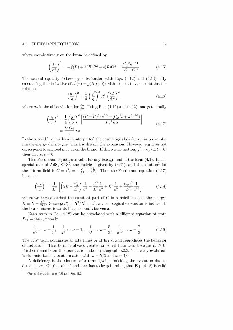
4.3. FRIEDMANN EQUATION 87
where cosmic time τ on the brane is defined by
(dτ
dt
)2
= −f(R) + h(R)R2 + s(R)Θ2 =f2g3e−2Φ
(E − C)2. (4.15)
The second equality follows by substitution with Eqs. (4.12) and (4.13). Bycalculating the derivative of a2(τ) = g(R(t(τ))) with respect to τ , one obtains therelation (aτ
a
)2
=1
4
(g′
g
)2
R2
(dt
dτ
)2
, (4.16)
where aτ is the abbreviation for dadτ . Using Eqs. (4.15) and (4.12), one gets finally
(aτ
a
)2
=1
4
(g′
g
)2 [(E − C)2s e2Φ − f(g3s+ J2e2Φ)
f g3 h s
]
≡ 8πG4
3ρeff .
(4.17)
In the second line, we have reinterpreted the cosmological evolution in terms of amirage energy density ρeff , which is driving the expansion. However, ρeff does notcorrespond to any real matter on the brane. If there is no motion, g ′ = dg/dR = 0,then also ρeff = 0.
This Friedmann equation is valid for any background of the form (4.1). In thespecial case of AdS5-S×S5, the metric is given by (3.61), and the solution1 for
the 4-form field is C = C4 = − r4
L4 +r4
H
2L4 . Then the Friedmann equation (4.17)becomes
(aτ
a
)2
=1
L2
[(2E +
r4HL4
)1
a4− J2
L2
1
a6+ E2 1
a8+r4HJ
2
L6
1
a10
], (4.18)
where we have absorbed the constant part of C in a redefinition of the energy:
E ≡ E − r4H
2L4 . Since g(R) = R2/L2 = a2, a cosmological expansion is induced ifthe brane moves towards bigger r and vice versa.
Each term in Eq. (4.18) can be associated with a different equation of statePeff = ωρeff , namely
1
a4↔ ω =
1
3,
1
a6↔ ω = 1,
1
a8↔ ω =
5
3,
1
a10↔ ω =
7
3. (4.19)
The 1/a4 term dominates at late times or at big r, and reproduces the behaviorof radiation. This term is always greater or equal than zero because E ≥ 0.Further remarks on this point are made in paragraph 5.2.3. The early evolutionis characterized by exotic matter with ω = 5/3 and ω = 7/3.
A deficiency is the absence of a term 1/a3, mimicking the evolution due todust matter. On the other hand, one has to keep in mind, that Eq. (4.18) is valid
1For a derivation see [93] and Sec. 5.2.
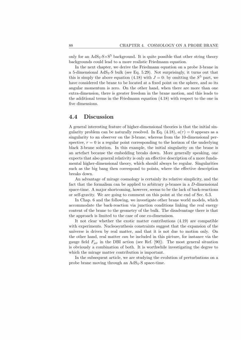
88 CHAPTER 4. COSMOLOGY ON A PROBE BRANE
only for an AdS5-S×S5 background. It is quite possible that other string theorybackgrounds could lead to a more realistic Friedmann equation.
In the next chapter, we derive the Friedmann equation on a probe 3-brane ina 5-dimensional AdS5-S bulk (see Eq. 5.29). Not surprisingly, it turns out thatthis is simply the above equation (4.18) with J = 0: by omitting the S5 part, wehave considered the brane to be located at a fixed point on the sphere, and so itsangular momentum is zero. On the other hand, when there are more than oneextra-dimension, there is greater freedom in the brane motion, and this leads tothe additional terms in the Friedmann equation (4.18) with respect to the one infive dimensions.
4.4 Discussion
A general interesting feature of higher-dimensional theories is that the initial sin-gularity problem can be naturally resolved. In Eq. (4.18), a(τ) = 0 appears as asingularity to an observer on the 3-brane, whereas from the 10-dimensional per-spective, r = 0 is a regular point corresponding to the horizon of the underlyingblack 3-brane solution. In this example, the initial singularity on the brane isan artefact because the embedding breaks down. More generally speaking, oneexpects that also general relativity is only an effective description of a more funda-mental higher-dimensional theory, which should always be regular. Singularitiessuch as the big bang then correspond to points, where the effective descriptionbreaks down.
An advantage of mirage cosmology is certainly its relative simplicity, and thefact that the formalism can be applied to arbitrary p-branes in a D-dimensionalspace-time. A major shortcoming, however, seems to be the lack of back-reactionsor self-gravity. We are going to comment on this point at the end of Sec. 6.3.
In Chap. 6 and the following, we investigate other brane world models, whichaccommodate the back-reaction via junction conditions linking the real energycontent of the brane to the geometry of the bulk. The disadvantage there is thatthe approach is limited to the case of one co-dimensison.
It not clear whether the exotic matter contributions (4.19) are compatiblewith experiments. Nucleosynthesis constraints suggest that the expansion of theuniverse is driven by real matter, and that it is not due to motion only. Onthe other hand, real matter can be included in this picture, for instance via thegauge field Fµν in the DBI action (see Ref. [90]). The most general situationis obviously a combination of both. It is worthwhile investigating the degree towhich the mirage matter contribution is important.
In the subsequent article, we are studying the evolution of perturbations on aprobe brane moving through an AdS5-S space-time.
Chapter 5
Perturbations on a movingD3-brane and miragecosmology (article)

90 CHAPTER 5. PERTURBATIONS ON A MOVING D3-BRANE
This chapter consists of the article ‘Perturbations on a moving D3-brane andmirage cosmology’, published in Phys.Rev.D66 (2002), see Ref. [22].
It is also available under http://lanl.arXiv.org/abs/hep-th/0206147.
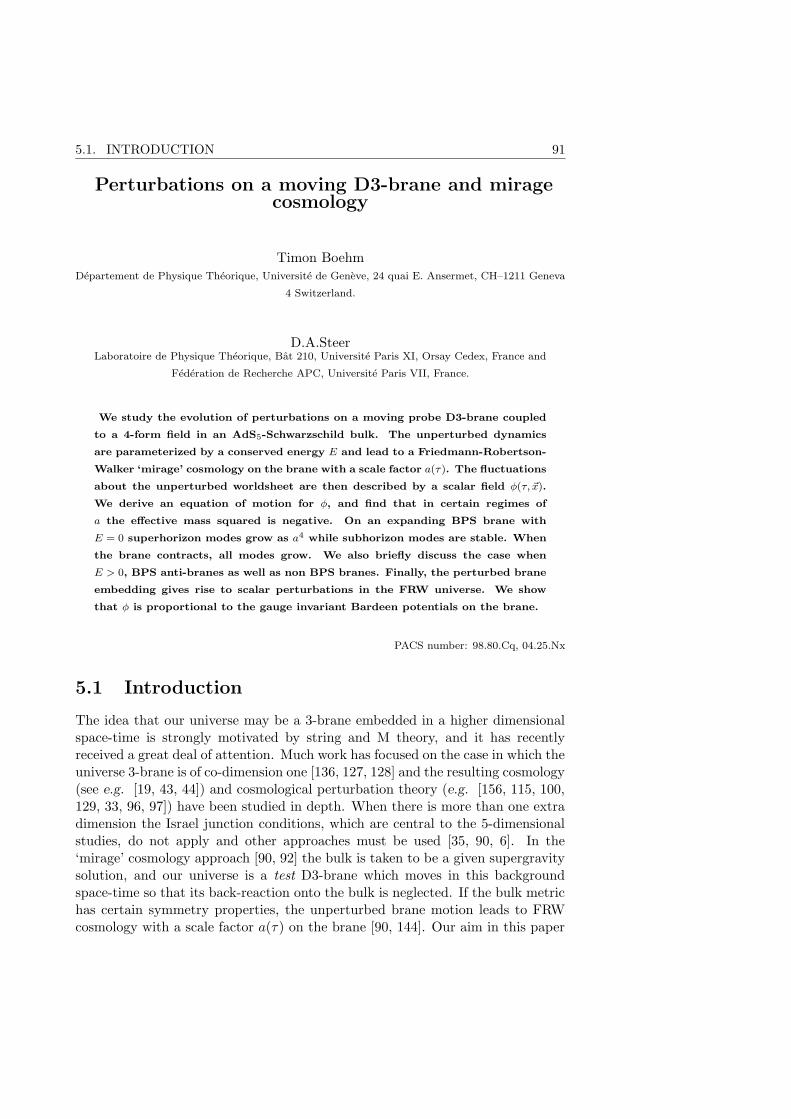
5.1. INTRODUCTION 91
Perturbations on a moving D3-brane and miragecosmology
Timon BoehmDepartement de Physique Theorique, Universite de Geneve, 24 quai E. Ansermet, CH–1211 Geneva
4 Switzerland.
D.A.SteerLaboratoire de Physique Theorique, Bat 210, Universite Paris XI, Orsay Cedex, France and
Federation de Recherche APC, Universite Paris VII, France.
We study the evolution of perturbations on a moving probe D3-brane coupled
to a 4-form field in an AdS5-Schwarzschild bulk. The unperturbed dynamics
are parameterized by a conserved energy E and lead to a Friedmann-Robertson-
Walker ‘mirage’ cosmology on the brane with a scale factor a(τ). The fluctuations
about the unperturbed worldsheet are then described by a scalar field φ(τ, ~x).
We derive an equation of motion for φ, and find that in certain regimes of
a the effective mass squared is negative. On an expanding BPS brane with
E = 0 superhorizon modes grow as a4 while subhorizon modes are stable. When
the brane contracts, all modes grow. We also briefly discuss the case when
E > 0, BPS anti-branes as well as non BPS branes. Finally, the perturbed brane
embedding gives rise to scalar perturbations in the FRW universe. We show
that φ is proportional to the gauge invariant Bardeen potentials on the brane.
PACS number: 98.80.Cq, 04.25.Nx
5.1 Introduction
The idea that our universe may be a 3-brane embedded in a higher dimensionalspace-time is strongly motivated by string and M theory, and it has recentlyreceived a great deal of attention. Much work has focused on the case in which theuniverse 3-brane is of co-dimension one [136, 127, 128] and the resulting cosmology(see e.g. [19, 43, 44]) and cosmological perturbation theory (e.g. [156, 115, 100,129, 33, 96, 97]) have been studied in depth. When there is more than one extradimension the Israel junction conditions, which are central to the 5-dimensionalstudies, do not apply and other approaches must be used [35, 90, 6]. In the‘mirage’ cosmology approach [90, 92] the bulk is taken to be a given supergravitysolution, and our universe is a test D3-brane which moves in this backgroundspace-time so that its back-reaction onto the bulk is neglected. If the bulk metrichas certain symmetry properties, the unperturbed brane motion leads to FRWcosmology with a scale factor a(τ) on the brane [90, 144]. Our aim in this paper
92 CHAPTER 5. PERTURBATIONS ON A MOVING D3-BRANE
is to study the evolution of perturbations on such a moving brane. Given theprobe nature of the brane, this question has many similarities with the studyof the dynamics and perturbations of topological defects such as cosmic strings[76, 64, 72, 16].
Though we derive the perturbation equations in a more general case, we con-sider in the end a bulk with AdS5-Schwarzschild×S5 geometry which is the nearhorizon limit of the 10-dimensional black D3-brane solution. In this limit (usingthe AdS-CFT correspondence) black-hole thermodynamics can be studied via theprobe D3-brane dynamics [36, 139]. As discussed in paragraph 5.2.1, we make theassumption that the D3-brane has no dynamics around the S5 so that the bulkgeometry is effectively AdS5-Schwarzschild. Because of the generalized Birkhofftheorem [26], this 5-dimensional geometry plays an important role in work onco-dimension one brane cosmology. Hence links can be made between the unper-turbed probe brane FRW cosmology discussed here and exact brane cosmologybased on the junction conditions [144]. Similarly, the perturbation theory westudy here is just one limit of the full, self-interacting and non Z2-symmetricbrane perturbation theory which has been studied elsewhere [129]. Commentswill be made in the conclusions regarding generalizations of this work to the full10-dimensional case.
Regarding the universe brane, the zeroth order (or background) solution istaken to be an infinitely straight brane whose motion is now constrained to bealong the single extra dimension labelled by coordinate r. The brane motion isparameterized by a conserved positive energy E [90]. In AdS5-Schwarzschild geo-metry and to an observer on the brane, the motion appears to be FRW expansionor contraction with a scale factor given by a ∝ r. Both the perturbed and un-perturbed brane dynamics will be obtained from the Dirac-Born-Infeld action fortype IIB superstring theory (see e.g. [14]),
SD3 = −T3
∫d4σ
√−det(gµν + 2πα′Fµν + Bµν)− ρ3
∫d4σ C4. (5.1)
Here σµ (µ = 0, 1, 2, 3) are coordinates on the brane world-sheet, T3 is the branetension, and in the second (Wess-Zumino) term ρ3 is the brane charge under aRamond-Ramond 4-form field living in the bulk. We will write
ρ3 = qT3, (5.2)
so that q = (−)1 for BPS (anti-)branes. In Eq. (5.1) gµν is the induced metric
and Fµν the field strength tensor of gauge fields on the brane. The quantities Bµν
and C4 are the pull-backs of the Neveu-Schwarz (NS) 2-form, and the Ramond-Ramond (RR) 4-form field in the bulk1. In the background we consider, the dila-ton is a constant and we set it to zero. In general the brane will not move slowly,and hence the square root in the DBI part of (5.1) may not be expanded: we will
1If we want to stress that a certain quantity is the pull-back of a bulk tensor, we use the widehatsymbol. However, for simplicity, we denote the induced metric by gµν rather than gµν
5.1. INTRODUCTION 93
consider the full non linear action. Finally, notice that since the 4-dimensionalRiemann scalar does not appear in (5.1) (and it is not inherited from the back-ground in this probe brane approach) there is no brane self-gravity. Hence the‘mirage’ cosmology we discuss here is solely sourced by the brane motion, and itleads to effects which are not present in 4-dimensional Einstein gravity. The lackof brane self-gravity is a serious limitation. However, in certain cases it may beincluded, for instance by compactifying the background space-time as discussedin [30] (see also [35]). Generally this leads to bi-metric theories. Even in thatcase, the mirage cosmology scale factor a(τ) which we discuss below plays animportant role and hence we believe it is of interest to study perturbations in this‘probe brane’ approach.
Deviations from the infinitely straight moving brane give rise to perturbationsaround the FRW solution. Are these ‘wiggles’ stretched away by the expansion,or on the contrary do they grow, leading to instabilities? To answer this ques-tion, we exploit the similarity with topological defects and make use of the workdeveloped in that context by Garriga and Vilenkin [64], Guven [72], and Battyeand Carter [16]. The perturbation dynamics are studied through a scalar fieldφ(σ) whose equation of motion is derived from the action (5.1). We find that, foran observer comoving with the brane, φ has a tachyonic mass in certain ranges ofr which depend on the conserved energy E characterizing the unperturbed branedynamics. We discuss the evolution of the modes φk for different E and show thatin many cases the brane is unstable. In particular, both sub and superhorizonmodes grow for a brane falling into the black-hole. It remains an open questionto see if brane self-gravity, neglected in this approach, can stabilize the system.
Finally, we also relate φ to the standard 4-dimensional gauge invariant scalarBardeen potentials Φ and Ψ on the brane. We find that Φ ∝ Ψ ∝ φ (no derivativesof φ enter into the Bardeen potentials).
The work presented here has some overlap with that of Carter et al. [41] whoalso studied perturbations on moving charged branes in the limit of negligibleself-gravity. Their emphasis was on trying to mimic gravity on the brane, and inaddition they included matter on the brane. Here we consider the simplest case inwhich there is no matter on the brane, namely Fµν = 0 in Eq. (5.1). Our focus ison studying the evolution of perturbations solely due to motion of the brane: weexpect the contribution of these perturbations to be important also when matteris included. Moreover, we hope that this study may more generally be of interestfor the dynamics and perturbations of moving D-branes in non BPS backgrounds.
The outline of the paper is as follows. In section 5.2 we link our 5-dimensionalmetric to the 10-dimensional black D3-brane solution and specify the unperturbedembedding of the probe brane. To determine its dynamics from the action (5.1)the bulk 4-form RR field must be specified. We discuss the normalization ofthis field. At the end of the section we summarize the motion of the probebrane by means of an effective potential. Comments are made regarding theFriedmann equation for an observer on the brane. In section 5.3 we consider smalldeviations from the background brane trajectory and investigate their evolution.
94 CHAPTER 5. PERTURBATIONS ON A MOVING D3-BRANE
The equation of motion for φ is derived, and we solve it in various regimes,commenting on the resulting instabilities. In section 5.4 we link φ to the scalarBardeen potentials on the brane. Finally, in section 5.5 we summarize our results.
5.2 Unperturbed dynamics of the D3-brane
In this section we discuss the background metric, briefly review the unperturbedD3-brane dynamics, and comment on the cosmology as seen by an observer on thebrane. The reader is referred to [90, 122] for a more detailed analysis on whichpart of this section is based.
5.2.1 Background metric and brane scale factor
For the reasons mentioned in the introduction, we focus mainly on an AdS5-S×S5 bulk space-time. This is closely linked to the 10-dimensional black 3-branesupergravity solution [78, 2, 93] which describes N coincident D3-branes carryingRR charge Q = NT3 and which is given by
ds210 = H−1/23 (−Fdt2 + d~x · d~x) +H
1/23
(dr2
F+ r2dΩ2
5
), (5.3)
where the coordinates (t, ~x) are parallel to the N D3-branes, dΩ25 is the line
element on a 5-sphere, and
H3(r) = 1 +L4
r4, F = 1− r4H
r4. (5.4)
The quantity L is the AdS5 curvature radius and the horizon rH vanishes whenthe ADM mass equals Q. The link between the metric parameters L, rH and thestring parameters N,T3 is given e.g. in [93]. The corresponding bulk RR fieldmay also be found in [93].
The near horizon limit of the metric (5.3) is AdS5-S×S5 space-time [2]. Ouruniverse is taken to be a D3-brane moving in this background. We make thefollowing two assumptions: first, the universe brane is a ‘probe’ so that its back-reaction on the bulk geometry is neglected. This may be justified if N À 1.Second, the probe is assumed to have no dynamics around S5 so that it is con-strained to move only along the radial direction r. This is a consistent solutionof the unperturbed dynamics since the brane has a conserved angular momentumabout the S5, and this may be set to zero [90, 144]. In section 5.3 we assume thatis also true for the perturbed dynamics. Thus in the remainder of this paper weconsider an AdS5-S bulk space-time with metric
ds25 = −f(r)dt2 + g(r)d~x · d~x+ h(r)dr2
≡ GMNdxMdxN ,(5.5)
5.2. UNPERTURBED DYNAMICS OF THE D3-BRANE 95
where (for r > rH)
f(r) =r2
L2
(1− r4H
r4
), g(r) =
r2
L2, h(r) =
1
f(r). (5.6)
In the limit rH → 0 this becomes pure AdS5.More generally, by symmetry, a stack of non rotating D3-branes generates a
metric of the form ds210 = ds25 + k(r)dΩ25, where ds25 is given in Eq. (5.5) [145].
In this case, since the metric coefficients are independent of the angular coordi-nates (θ1, · · · , θ5), the unperturbed brane dynamics are always characterized bya conserved angular momentum around the S5 [90]. As a result of the second as-sumption above, we are thus effectively led to consider metrics of the form (5.5).Hence, for the derivation of both the unperturbed and perturbed equations ofmotion, we keep f, g, h arbitrary and consider the specific form (5.6) only at theend.
The embedding of the probe D3-brane is given by xM = XM(xµ). (We haveused reparametrization invariance to choose the intrinsic worldsheet coordinatesσµ = xµ.) For the unperturbed trajectory we consider an infinitely straight braneparallel to the xµ hyperplane but free to move along the r direction:
Xµ = xµ, X4 = R(t). (5.7)
Later, in section 5.3, we will consider a perturbed brane for which X 4 = R(t) +δR(t, ~x).
The induced metric on the brane is given by
gµν = GMN(X)∂XM
∂xµ
∂XN
∂xν, (5.8)
so that the line element on the unperturbed brane worldsheet is
ds24 = gµνdxµdxν = −(f(R)− h(R)R2)dt2 + g(R)d~x · d~x ≡ −dτ 2 + a2(τ)d~x · d~x.(5.9)
An observer on the brane therefore sees a homogeneous and isotropic universe inwhich the time τ and the scale factor a(τ) are given by
τ =
∫ √(f − hR2)dt, a(τ) =
√g(R(τ)). (5.10)
The properties of the resulting Friedmann equation depend on f(R), g(R), h(R)(i.e. the bulk geometry) as well as R (the brane dynamics) as discussed in [90, 144]and summarized briefly below.
5.2.2 Brane action and bulk 4-form field
In AdS5-S geometry, BMN vanishes, and we do not consider the gauge field Fµν
on the brane. (For a detailed discussion of the unperturbed brane dynamics with
96 CHAPTER 5. PERTURBATIONS ON A MOVING D3-BRANE
and without Fµν , which essentially corresponds to radiation on the brane, see[90, 144]. Non zero BMN has been discussed in [163].) Thus the brane action(5.1) reduces to
SD3 = −T3
∫d4x√−g − ρ3
∫d4x C4, (5.11)
where
g = det(gµν), C4 = CMNSR
∂XM
∂x0
∂XN
∂x1
∂XS
∂x2
∂XR
∂x3, (5.12)
and CMNSR are components of the bulk RR 4-form field. The first term inEq. (5.11) is just the Nambu-Goto action.
In the gauge (5.7), g and C4 depend on t only through R. Thus rather thanvarying (5.11) with respect to XM and then integrating the equations of motion,it is more straightforward to obtain the equations of motion from the Lagrangian
L = −√−g − C = −√fg3 − g3hR2 − C, (5.13)
where C = C(R) = ρ3
T3C4 = qC4. Since L does not explicitly depend on time, the
brane dynamics are parameterized by a (positive) conserved energy E = ∂L∂RR−L
from which
R2 =f
h
(1− fg3
(E − C)2
). (5.14)
Transforming to brane time τ defined in equation (5.10) yields
R2τ =
(E − C)2
fg3h− 1
h, (5.15)
where the subscript denotes a derivative with respect to τ .
In order to analyze the brane dynamics in AdS5-S space-time, where f, g andh are given in Eq. (5.6), one must finally specify C(R) or equivalently the 4-formpotential CMNSR. To that end2 recall that the 5-dimensional bulk action is
S5 =1
2κ25
∫d5x√−G(R− 2Λ)− 1
4κ25
∫F5 ∧ ∗F5, (5.16)
where Λ is the bulk cosmological constant3 and F5 = dC4 is the 5-form field
2For the 10-dimensional AdS5-S×S5 geometry the solution for the 4-form field is given, for exam-ple, in [93]. For completeness, we rederive the result starting directly from the 5-dimensional metric(5.6).
3Note that there is no cosmological constant in the fundamental 10-dimensional supergravityaction 2.1. Here, Λ appears because we consider only the AdS5 part. It represents the negativecosmological constant of AdS5 which, together with the positive Ricci curvature form the 5-sphere,adds up to zero. Thus Λ is needed for consistency of the equations of motion.
5.2. UNPERTURBED DYNAMICS OF THE D3-BRANE 97
strength associated with the 4-form C4. The resulting equations of motion are
RMN =2
3ΛGMN +
1
2 · 4!
(FMBCDEFN
BCDE − 4
3 · 5FABCDEFABCDEGMN
),
(5.17)
d ∗ F5 =1
2
1√fg3h
((f ′
f+ 3
g′
g+h′
h
)F01234 − 2F ′
01234
)dr = 0, (5.18)
where the prime denotes a derivative with respect to r. In AdS5-S, RMN =− 4
L2GMN and Eq. (5.18) gives
L3
r3
(3
rF01234 − F ′
01234
)= 0 =⇒ F01234 = c
r3
L4, (5.19)
where c is a dimensionless constant (see for example [40]). (Note that this solutionsatisfies dF5 = 0 since the only non zero derivative is ∂4F01234 which vanishes onantisymmetrizing.) Integration gives
C0123 = vr4
L4+ w, (5.20)
where v = c/4 and w are again dimensionless constants. Hence the function C(r)appearing in Eq. (5.13) is
C(r) = qC0123 = qvr4
L4+ qw. (5.21)
In 10 dimensions the constant c (and hence v) is fixed by the condition∫∗F =
Q , and w may be determined by imposing (before taking the near horizon limitand hence with metric (5.3)) that the 4-form potential should die off at infinity[93]. This second argument is not applicable here. Instead, we fix v and w inthe following way: consider the motion of the unperturbed brane seen by a bulkobserver with time coordinate t. One can define an effective potential V t
eff through
1
2R2 + V t
eff ≡ E (5.22)
so that on using equation (5.14),
V teff(E, q,R) = E − 1
2
(R
L
)4
α2
[1−
(R
L
)8α
(E − C)2
](5.23)
(see Fig. 5.2) where
α = 1− r4HR4
,
and C = C(R) is given in Eq. (5.21). We now use the fact that there is no netforce between static BPS objects of like charge, and hence in this case the effective
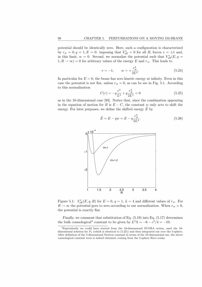
98 CHAPTER 5. PERTURBATIONS ON A MOVING D3-BRANE
potential should be identically zero. Here, such a configuration is characterizedby rH = 0, q = 1, E = 0: imposing that V t
eff = 0 for all R, forces v = ±1 and,in this limit, w = 0. Second, we normalize the potential such that V t
eff(E, q =1, R→∞) = 0 for arbitrary values of the energy E and rH . This leads to
v = −1, w = +r4H2L4
. (5.24)
In particular for E = 0, the brane has zero kinetic energy at infinity. Even in thiscase the potential is not flat, unless rH = 0, as can be see in Fig. 5.1. Accordingto this normalization
C(r) = −q r4
L4+ q
r4H2L4
< 0 (5.25)
as in the 10-dimensional case [93]. Notice that, since the combination appearingin the equation of motion for R is E − C, the constant w only acts to shift theenergy. For later purposes, we define the shifted energy E by
E = E − qw = E − q r4H
2L4. (5.26)
1 1.5 2 2.5 3 3.5 4
−2
−1
0 x 10−4
R
rH=1
rH=1.2
Figure 5.1: V teff(E, q,R) for E = 0, q = 1, L = 4 and different values of rH . For
R→∞ the potential goes to zero according to our normalization. When rH = 0,the potential is exactly flat.
Finally, we comment that substitution of Eq. (5.19) into Eq. (5.17) determinesthe bulk cosmological4 constant to be given by L2Λ = −6− c2/4 = −10.
4Equivalently we could have started from the 10-dimensional SUGRA action, used the 10-dimensional solution for F5 (which is identical to (5.25)) and then integrated out over the 5-sphere.After definition of the 5-dimensional Newton constant in terms of the 10-dimensional one, the abovecosmological constant term is indeed obtained, coming from the 5-sphere Ricci scalar.
5.2. UNPERTURBED DYNAMICS OF THE D3-BRANE 99
5.2.3 Brane dynamics and Friedmann equation
We now make some comments regarding the unperturbed motion of the 3-branethrough the bulk, R(τ), as seen by an observer on the brane. This will be usefulin section 5.3 when discussing perturbations. Recall that since a(τ) = R(τ)/L(see Eq. (5.10)), an ‘outgoing’ brane leads to cosmological expansion. Contractionoccurs when the brane moves inward. For the observer on the brane, one maydefine an effective potential by
1
2Rτ
2 + V τeff = E, (5.27)
whence, from Eq. (5.15),
V τeff(E, q,R) = E +
1
2
(L
R
)6[α
(R
L
)8
− (E − C)2
]. (5.28)
Consider a BPS brane q = +1 (see Fig. 5.3). As noted above, for rH = E = 0one has V τ
eff = 0 so that the potential is flat. For rH 6= 0, V τeff contains a term
∝ −R−6, and the probe brane accelerates toward the horizon, which is reachedin finite (τ -)time. On the other hand, for a bulk observer with time t, it takesinfinite time to reach the horizon where V t
eff = E (see Fig. 5.2).From Eqs. (5.15) and (5.21) it is straightforward to derive a Friedmann-like
equation for the brane scale factor a(τ) [90, 144]:
H2 =(aτ
a
)2
=1
L2
[E2
a8+
1
a4
(2qE +
r4HL4
)+ (q2 − 1)
]. (5.29)
The term in 1/a8 (a ‘dark fluid’ with equation of state P = 5/3ρ) dominates atearly times. The second term in 1/a4 is a ‘dark radiation’ term. As discussed in[144], the part proportional to rH corresponds to the familiar dark radiation termin conventional Z2-symmetric (junction condition) brane cosmology, where it isassociated with the projected bulk Weyl tensor. When E is non zero, Z2 symmetryis broken5 [144] and this leads to a further dark radiation term [40, 98]. Thelast term in Eq. (5.29) defines an effective 4-dimensional cosmological constantΛ4
3 ≡ 1L2 (q2−1) which vanishes if the (anti) brane is BPS (i.e. q = ±1). All these
terms have previously been found in both mirage cosmology and conventionalbrane cosmology [144, 40].
Notice that the dark radiation term above has a coefficient
µ ≡ 2qE +r4HL4
= 2qE − r4HL4
(q2 − 1), (5.30)
which is positive for q = +1 (since E ≥ 0). However, for BPS anti-branes q = −1,the coefficient (5.30) is negative unless E = 0. Thus when E 6= 0 and q = −1
5When making the link between mirage cosmology and the junction condition approach, E ∝M− − M+ where M± are the black-hole masses on each side of the brane [144].
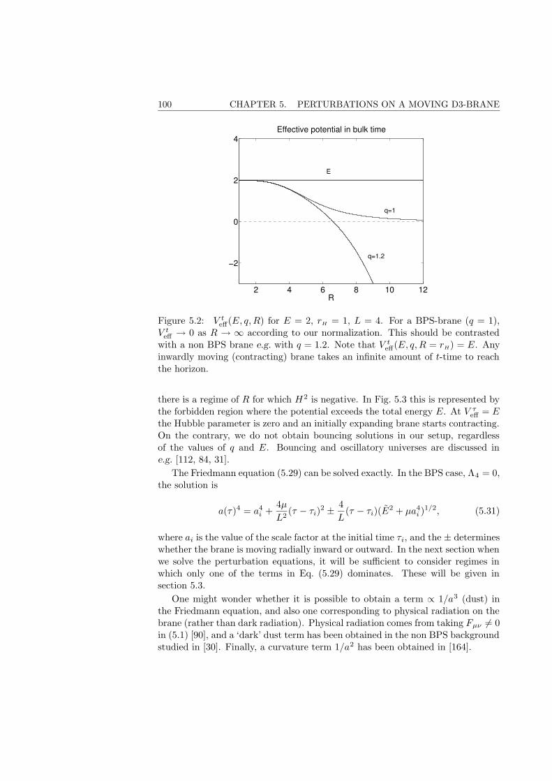
100 CHAPTER 5. PERTURBATIONS ON A MOVING D3-BRANE
2 4 6 8 10 12
−2
0
2
4
R
Effective potential in bulk time
E
q=1
q=1.2
Figure 5.2: V teff(E, q,R) for E = 2, rH = 1, L = 4. For a BPS-brane (q = 1),
V teff → 0 as R → ∞ according to our normalization. This should be contrasted
with a non BPS brane e.g. with q = 1.2. Note that V teff(E, q,R = rH) = E. Any
inwardly moving (contracting) brane takes an infinite amount of t-time to reachthe horizon.
there is a regime of R for which H2 is negative. In Fig. 5.3 this is represented bythe forbidden region where the potential exceeds the total energy E. At V τ
eff = Ethe Hubble parameter is zero and an initially expanding brane starts contracting.On the contrary, we do not obtain bouncing solutions in our setup, regardlessof the values of q and E. Bouncing and oscillatory universes are discussed ine.g. [112, 84, 31].
The Friedmann equation (5.29) can be solved exactly. In the BPS case, Λ4 = 0,the solution is
a(τ)4 = a4i +
4µ
L2(τ − τi)2 ±
4
L(τ − τi)(E2 + µa4
i )1/2, (5.31)
where ai is the value of the scale factor at the initial time τi, and the ± determineswhether the brane is moving radially inward or outward. In the next section whenwe solve the perturbation equations, it will be sufficient to consider regimes inwhich only one of the terms in Eq. (5.29) dominates. These will be given insection 5.3.
One might wonder whether it is possible to obtain a term ∝ 1/a3 (dust) inthe Friedmann equation, and also one corresponding to physical radiation on thebrane (rather than dark radiation). Physical radiation comes from taking Fµν 6= 0in (5.1) [90], and a ‘dark’ dust term has been obtained in the non BPS backgroundstudied in [30]. Finally, a curvature term 1/a2 has been obtained in [164].
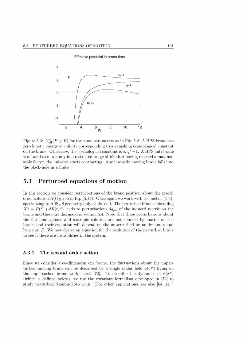
5.3. PERTURBED EQUATIONS OF MOTION 101
2 4 6 8 10 12
−4
−2
0
2
4
R
Effective potential in brane time
E q=−1
q=1
q=1.2
Figure 5.3: V τeff(E, q,R) for the same parameters as in Fig. 5.2. A BPS brane has
zero kinetic energy at infinity corresponding to a vanishing cosmological constanton the brane. Otherwise, the cosmological constant is ∝ q2−1. A BPS anti-braneis allowed to move only in a restricted range of R: after having reached a maximalscale factor, the universe starts contracting. Any inwardly moving brane falls intothe black-hole in a finite τ .
5.3 Perturbed equations of motion
In this section we consider perturbations of the brane position about the zerothorder solution R(t) given in Eq. (5.14). Once again we work with the metric (5.5),specializing to AdS5-S geometry only at the end. The perturbed brane embeddingX4 = R(t) + δR(t, ~x) leads to perturbations δgµν of the induced metric on thebrane and these are discussed in section 5.4. Note that these perturbations aboutthe flat homogenous and isotropic solution are not sourced by matter on thebrane, and their evolution will depend on the unperturbed brane dynamics andhence on E. We now derive an equation for the evolution of the perturbed braneto see if there are instabilities in the system.
5.3.1 The second order action
Since we consider a co-dimension one brane, the fluctuations about the unper-turbed moving brane can be described by a single scalar field φ(xµ) living onthe unperturbed brane world sheet [72]. To describe the dynamics of φ(xµ)(which is defined below), we use the covariant formalism developed in [72] tostudy perturbed Nambu-Goto walls. (For other applications, see also [64, 34].)
102 CHAPTER 5. PERTURBATIONS ON A MOVING D3-BRANE
The perturbed brane embedding is given by
XM(t, ~x) = XM(t) + φ(t, ~x)nM(t), (5.32)
where XM(t) is the unperturbed embedding, and physical perturbations are onlythose transverse to the brane (see also section 5.4). The unit space-like normalto the unperturbed brane, nM(t) = nM(X(t)), is defined through
GMNnM∂XN
∂xµ= 0, GMNn
MnN = 1, (5.33)
so that
nM =
(R
√h
f(f − hR2), 0, 0, 0,
√f
h(f − hR2)
). (5.34)
Thus for a 5-dimensional observer comoving with the brane, φ (which has dimen-sions of length) is the measured deviation from the background solution of theprevious section [64]. For an observer living on the brane, the perturbations inthe FRW metric generated by φ are discussed in section 5.4 in terms of the gaugeinvariant scalar Bardeen potentials.
An equation of motion for φ can be obtained by substituting (5.32) into theaction (5.11) and expanding to second order in φ. The terms linear in φ give thebackground (unperturbed) equations of motion studied in the previous section;now we are interested in the terms quadratic in φ which give the linearized equa-tions of motion. A similar analysis was carried out by Garriga and Vilenkin [64]for Nambu-Goto cosmic domain walls in Minkowski space and was generalized byGuven [72] for arbitrary backgrounds. For the action (5.11), the quadratic termis [34]
Sφ2 = −1
2
∫d4x√−g
[(∇µφ)(∇µφ)− (kµ
νkν
µ +RMNnMnN)φ2
]. (5.35)
Here ∇ is the covariant derivative with respect to the induced metric gµν , andthe extrinsic curvature tensor kµν on the brane is given by
kµν = −(∇NnM)∂XM
∂xµ
∂XN
∂xν, (5.36)
where ∇ is the covariant derivative with respect to the 5-dimensional metric GMN .Finally, RMN is the Ricci tensor of the metric GMN . Apart from φ, all the terms in(5.35) are unperturbed quantities. Note that there is no contribution to Sφ2 fromthe Wess-Zumino term of the action (5.11): all terms quadratic in φ cancel sinceC0123 is the only non zero component of the 4-form field. However, C does enterinto the term linear in φ and hence into the background equations of motion, asanalyzed in the previous sections.
Variation of the action (5.35) with respect to φ leads to the equation of motion
∇µ∇µφ+ (kµνk
νµ +RMNn
MnN)φ = 0 (5.37)
5.3. PERTURBED EQUATIONS OF MOTION 103
or equivalently∇µ∇µφ−m2φ = 0, (5.38)
wherem2 = − (kµ
νkν
µ +RMNnMnN) . (5.39)
To determine the extrinsic curvature contribution to (5.39), it is simpler to cal-culate first the 5-dimensional extrinsic tensor or second fundamental form definedby Eq. (3.22)
KMN = −qB
NqC
M∇CnB, (5.40)
where qBN acts as projection tensor onto the brane. It is the mixed tensor asso-
ciated with the first fundamental form
qMN = GMN − nMnN . (5.41)
We then use the fact that
kµνk
νµ = KM
NKN
M . (5.42)
On defining T by
T ≡(
dτ
dt
)2
= f − hR2 =f2g3
(E − C)2, (5.43)
the non zero components of KMN are
K00 = − 1
T 5/2f3/2h1/2
(R− f ′
fR2 +
1
2
h′
hR2 +
1
2
f ′
h
), (5.44)
K04 =
hR
fK0
0, (5.45)
K11 = − 1
T 1/2
(f
h
)1/21
2
g′
g= K2
2 = K33, (5.46)
K44 =
hR2
fK0
0 (5.47)
so that
kµνk
νµ = KM
NKN
M =1
T
f
h
[3
(g′
g
)2
+ 3g′
g
C ′
E − C +
(C ′
E − C
)2]. (5.48)
The Ricci term is
RMNnMnN = − 1
4h
[2f ′′
f−(f ′
f
)2
+ 3f ′
f
g′
g− f ′
f
h′
h
]
+3
4
1
T
f
h
[f ′
f
g′
g− 2
g′′
g+
(g′
g
)2
+g′
g
h′
h
].
(5.49)
104 CHAPTER 5. PERTURBATIONS ON A MOVING D3-BRANE
Collecting these results gives
m2 = −3
4
(E − C)2
fg3h
[f ′
f
g′
g− 2
g′′
g+ 5
(g′
g
)2
+g′
g
h′
h+ 4
g′
g
C ′
E − C
+4
3
(C ′
E − C
)2]
+1
4h
[2f ′′
f−(f ′
f
)2
+ 3f ′
f
g′
g− f ′
f
h′
h
].
(5.50)
In the remainder of this section we try to obtain approximate solutions for φfrom equation (5.38). Some aspects of this calculation are clearer in brane timeτ , and others in conformal time η (where η =
∫dτ/a(τ)). Of course the results
are independent of the coordinate system. For these reasons we have decided topresent both approaches, beginning with brane time.
5.3.2 Evolution of perturbations in brane time τ
On using the definition of brane time τ in equation (5.10), the kinetic term in(5.37) is given by
∇µ∇µφ = −φττ − 3Hφτ +1
a2(φx1x1 + φx2x2 + φx3x3) . (5.51)
(In conformal time the factor of a−2 multiplying the spatial derivatives disappears,see below.) We now change variables to ϕ = a3/2φ so that Eq. (5.38) becomes
ϕττ −1
a2(ϕx1x1 + ϕx2x2 + ϕx3x3) +M2(τ)ϕ = 0, (5.52)
where
M2(τ) = m2 − 3
4
[(aτ
a
)2
+ 2aττ
a
]
= m2 − 3
4
[g′′
gR2
τ −1
4
(g′
g
)2
R2τ +
g′
gRττ
]
=3
4
(E − C)2
fg3h
[− 1
2
f ′
f
g′
g+g′′
g− 13
4
(g′
g
)2
− 1
2
g′
g
h′
h− 3
g′
g
C ′
E − C
− 4
3
(C ′
E − C
)2]
+1
4h
[2f ′′
f−(f ′
f
)2
+ 3f ′
f
g′
g− f ′
f
h′
h+ 3
g′′
g− 3
4
(g′
g
)2
− 3
2
g′
g
h′
h
].
(5.53)
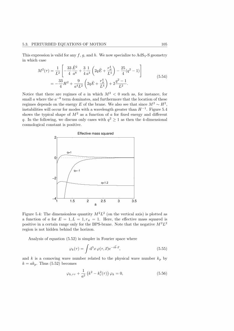
5.3. PERTURBED EQUATIONS OF MOTION 105
This expression is valid for any f , g, and h. We now specialize to AdS5-S geometryin which case
M2(τ) =1
L2
[−33
4
E2
a8+
3
4
1
a4
(2qE +
r4HL4
)− 25
4(q2 − 1)
]
= −33
4H2 +
9
a4L2
(2qE +
r4HL4
)+ 2
q2 − 1
L2.
(5.54)
Notice that there are regimes of a in which M 2 < 0 such as, for instance, forsmall a where the a−8 term dominates, and furthermore that the location of theseregimes depends on the energy E of the brane. We also see that since M 2 ∼ H2,instabilities will occur for modes with a wavelength greater than H−1. Figure 5.4shows the typical shape of M 2 as a function of a for fixed energy and differentq. In the following, we discuss only cases with q2 ≥ 1 as then the 4-dimensionalcosmological constant is positive.
1 1.5 2 2.5 3 3.5−4
−2
0
2
a
Effective mass squared
q=1
q=−1
q=1.2
Figure 5.4: The dimensionless quantity M 2L2 (on the vertical axis) is plotted asa function of a for E = 1, L = 1, rH = 1. Here, the effective mass squared ispositive in a certain range only for the BPS-brane. Note that the negative M 2L2
region is not hidden behind the horizon.
Analysis of equation (5.52) is simpler in Fourier space where
ϕk(τ) =
∫d3xϕ(τ, ~x)e−i~k·~x, (5.55)
and k is a comoving wave number related to the physical wave number kp byk = akp. Thus (5.52) becomes
ϕk,ττ +1
a2
(k2 − k2
c (τ))ϕk = 0, (5.56)
106 CHAPTER 5. PERTURBATIONS ON A MOVING D3-BRANE
where the time dependent critical wave number k2c (τ) is given by
k2c (τ) = −M2(τ)a2. (5.57)
One might suppose that for M 2 > 0 all modes are stable. However, due tothe τ -dependence of kc this is not necessarily true (as we shall see in equation(5.71)).
Our aim now is to determine the a-dependence of ϕk. We proceed in thefollowing way: notice first that the Friedmann equation (5.29) and the expressionfor M2(τ) in (5.54) both contain terms in a−8, a−4, and a0. We will focus ona regime in which one of these terms dominates. Then the Friedmann equationcan be solved for a(τ) which, on substitution into (5.54), gives M 2(τ). A finalsubstitution of M 2(τ) into the perturbation equation (5.56) for ϕk enables thisequation to be solved in each regime. We consider the following cases: i) q = +1,ii) q = −1 and iii) q2 > 1.
BPS brane: q = +1
For a BPS brane, the Friedmann equation (5.29) and effective mass M 2(τ) aregiven by
H2 =1
L2
[E2
a8+
2E
a4
], (5.58)
M2(τ) =1
L2
[−33
4
E2
a8+
3
2
E
a4
]. (5.59)
The E dependence of these equations slightly complicates the analysis of theseequations, and hence we begin with the simplest case in which E = 0.
Case 1 E = 0:
When E = 0 (the static limit in which the probe has zero kinetic energy atinfinity (see Fig. 5.1)) only the term proportional to a−8 survives in (5.58) and(5.59). Recall that when rH vanishes the potential V τ
eff is flat. Furthermore, sinceE ∝ r4H = 0, it follows from (5.59) that M 2(τ) = 0 in this limit: as expected, aBPS probe brane with zero energy in AdS5 has no dynamics and is completelystable.
When rH 6= 0, M2(τ) < 0 ∀τ , and the solution of (5.58) is
a(τ)4 = a4i ±
2a4H
L(τ − τi). (5.60)
Here ai ≥ aH ≡ rH/L is the initial position of the brane at τ = τi, and thechoice of sign determines whether the brane is moving radially inward (−) oroutward (+): this is a question of initial conditions. Let Rh = 1/|Ha| denote the
5.3. PERTURBED EQUATIONS OF MOTION 107
(comoving) Hubble radius. Then it follows from (5.59) and the definition of k2c in
(5.57) that1
λc∼ |kc(τ)| ∼ |Ha| =
1
Rh, (5.61)
where we neglect numerical factors of order 1. Thus the critical wavelength isλc ∼ Rh. (Notice that Rh is minimal at aH and increases with a.)
For superhorizon modes λÀ Rh or |k| ¿ |kc|, and in this limit the perturba-tion equation (5.56) becomes
ϕk,ττ −k2
c (τ)
a2ϕk = 0. (5.62)
On inserting solution (5.60) into k2c one obtains
φk =ϕk
a3/2= Aka
4 +Bka−3, (5.63)
(where the constants Ak and Bk are determined by the initial conditions). Henceif the brane moves radially outward the superhorizon modes grow as a4 ∝ τ . Ifthe brane is contracting they grow as a−3. In the near extremal limit, rH ¿ Lor aH ¿ 1, the amplitude of these superhorizon modes can become very large,suggesting that they are unstable. Of course our linear analysis will break downwhen φ becomes too large.
Consider now subhorizon modes λ ¿ Rh or |k| À |kc|. Then (5.56) is justϕk,ττ +
(k2/a2
)ϕk = 0. However, in this case it is much easier to solve the
equation in conformal time η where the factor of a−2 is no longer present. Weanticipate the result from paragraph 5.3.3: it is
φk = Akeikη
a+Bk
e−ikη
a. (5.64)
For an outgoing brane a increases and subhorizon modes are stable. For an ingoingbrane a decreases, and the amplitude of the perturbation becomes very large inthe near extremal limit. (Note that, as the brane expands, superhorizon modeseventually become subhorizon, and similarly, on a contracting brane, subhorizonmodes become superhorizon.)
To conclude, when rH 6= 0, E = 0, and the brane expands, superhorizon modesare unstable while subhorizon modes are stable. For a contracting brane, and inthe near extremal limit, both super and subhorizon modes are unstable.
Case 2 E 6= 0:When the energy of the brane is non zero the situation is more complicated.
Notice first from (5.59) that M 2(τ) has one zero at a = ac given by
a4c =
11E2
2E. (5.65)
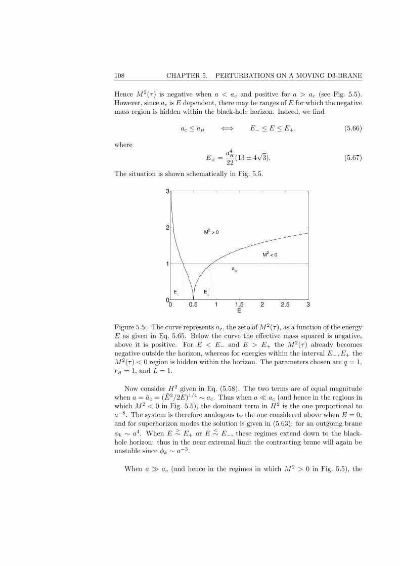
108 CHAPTER 5. PERTURBATIONS ON A MOVING D3-BRANE
Hence M2(τ) is negative when a < ac and positive for a > ac (see Fig. 5.5).However, since ac is E dependent, there may be ranges of E for which the negativemass region is hidden within the black-hole horizon. Indeed, we find
ac ≤ aH ⇐⇒ E− ≤ E ≤ E+, (5.66)
where
E± =a4
H
22(13± 4
√3). (5.67)
The situation is shown schematically in Fig. 5.5.
0 0.5 1 1.5 2 2.5 30
1
2
3
E
E−
E+
M2 > 0
M2 < 0
aH
Figure 5.5: The curve represents ac, the zero ofM2(τ), as a function of the energyE as given in Eq. 5.65. Below the curve the effective mass squared is negative,above it is positive. For E < E− and E > E+ the M2(τ) already becomesnegative outside the horizon, whereas for energies within the interval E−, E+ theM2(τ) < 0 region is hidden within the horizon. The parameters chosen are q = 1,rH = 1, and L = 1.
Now consider H2 given in Eq. (5.58). The two terms are of equal magnitudewhen a = ac = (E2/2E)1/4 ∼ ac. Thus when a¿ ac (and hence in the regions inwhich M2 < 0 in Fig. 5.5), the dominant term in H2 is the one proportional toa−8. The system is therefore analogous to the one considered above when E = 0,and for superhorizon modes the solution is given in (5.63): for an outgoing brane
φk ∼ a4. When E>∼ E+ or E
<∼ E−, these regimes extend down to the black-hole horizon: thus in the near extremal limit the contracting brane will again beunstable since φk ∼ a−3.
When a À ac (and hence in the regimes in which M 2 > 0 in Fig. 5.5), the
5.3. PERTURBED EQUATIONS OF MOTION 109
dominant term in H2 is ∝ a−4 so that
a(τ)2 = a2i ± 2
√2E
L(τ − τi) (5.68)
and
k2c (τ) = −M2(τ)a2 = −3
2
E
L2a2. (5.69)
On superhorizon scales the mode equation is
ϕk,ττ +3
2
E
L2a4ϕk = 0. (5.70)
At first sight one might expect the solution to this equation to be stable sinceM2 > 0. However, surprisingly, it is not. (Indeed, below we will see that inconformal time the effective mass is actually negative in this regime.) A changeof variables to u = a2 shows that the solution of (5.70) is
ϕk = Aka3/2 +Bka
1/2 (5.71)
which grows as τ 3/4, τ1/4 respectively. Finally,
φk = Ak +Bka−1. (5.72)
For E within the band E−<∼ E
<∼ E+, the solution (5.72) for the modes is validfor all a so that superhorizon modes grow as a−1 as the brane approaches theblack-hole horizon.
When E>∼ E+ or E
<∼ E− these solutions are valid for a À ac. Thus foran expanding brane φk tends to a constant value. For a contracting brane, theterm ∝ a−1 could become important, although for small enough a the relevantregime is that considered above in which case the solution is given by (5.63) andthe superhorizon modes grow as a−3.
For subhorizon modes, the solution is still as given in (5.64).
BPS anti-branes: q = −1
Now the Friedmann equation (5.29) and effective mass M 2(τ) become
H2 =1
L2
[E2
a8− 2E
a4
], (5.73)
M2(τ) = − 1
L2
[33
4
E2
a8+
3
2
E
a4
](5.74)
so that M2 is always negative, independently of E. Note that H2 > 0 for a < ac
where ac = (E2/2E)1/4. However, since E = E + a4H/2 for anti-branes, it follows
that ac ≥ aH for all E (i.e. there are no energy bands to consider in the case ofanti-branes). When a ¿ ac, H
2 ∝ M2 ∝ a−8 and once again this is analogousto the case studied above for E = 0: superhorizon modes grow as a4, and in thenear extremal limit the subhorizon modes on an ingoing brane are unstable.
110 CHAPTER 5. PERTURBATIONS ON A MOVING D3-BRANE
Non BPS branes: q 6= ±1
Here we shall only briefly discuss the case q2 > 1 for large a. Now, independentlyof E, there is a cosmological constant dominated regime (see Eq. (5.29)). Therethe solution for the scale factor is
a(τ) = a(τi)e±√
Λ4/3(τ−τi) whereΛ4
3≡ q2 − 1
L2. (5.75)
In this regime, however, M 2 is negative with
M2(τ) = −25
12Λ4 (5.76)
and Rh = 1/|Ha| = (Λ4/3)−1/2
a−1.
For subhorizon modes (λ ¿ Rh) the solution for ϕk is again given by (5.64).For superhorizon modes, and considering an outgoing brane, there is an exponen-tially growing unstable mode
φk = Ake√
Λ4/3(τ−τi) = Aka. (5.77)
Hence, this non BPS brane is unstable for large a. It is not clear to us why theacceleration due to the positive cosmological constant does not rather stretch theperturbations away.
5.3.3 Comments on an analysis in conformal time η
It is instructive to carry out a similar analysis in conformal time η rather thancosmic time τ , and we comment briefly on it here. In conformal time and trans-formed to Fourier space, Eq. (5.38) becomes
φk,ηη + 2Hφk,η + (k2 + a2m2)φk = 0, (5.78)
where H = aH. The friction term can be eliminated by a change of variables toψ = aφ, and the above equation becomes
ψk,ηη +(k2 − k2
c (η))ψk = 0, (5.79)
where
k2c (η) = −M2(η)
5.3. PERTURBED EQUATIONS OF MOTION 111
and
M2(η) = a2m2 − aηη/a
= gm2 +1
2
[−g
′′
gR2
η +1
2
(g′
g
)2
R2η −
g′
gRηη
]
= −(E − C)2
fg2h
[1
2
f ′
f
g′
g− g′′
g+ 3
(g′
g
)2
+1
2
g′
g
h′
h+
5
2
g′
g
C ′
E − C
+
(C ′
E − C
)2]
+g
2h
[f ′′
f− 1
2
(f ′
f
)2
+3
2
f ′
f
g′
g− 1
2
f ′
f
h′
h+g′′
g− 1
2
g′
g
h′
h
].
(5.80)
Specializing to AdS5-S yields
M2(η) = − 1
L2
[10E2
a6+ 6(q2 − 1)a2
]. (5.81)
Notice that in conformal time and for |q| ≥ 1,M2(η) is always negative inde-pendently of E. From this, one can immediately see the instability for small k inEq. (5.71), even though M 2(τ) can be positive in that case. It is clear that theresults on brane (in)stability must be independent of whether or not the analysisis carried out in η or τ time. We will see that this is indeed the case: the reasonis that not only the sign of the effective mass squared but also its functional de-pendence on time determine the stability properties. We now summarize brieflysome of the aspects that differ between the τ and η analysis.
Consider the simplest case: q = +1 and E = 0. The solution of the (conformaltime) Friedmann equation is a3 = a3
i ± 3a2H(η− ηi)/2L, and kc(η) ∼ |H| = 1/Rh.
For superhorizon modes |k| ¿ |kc| Eq. (5.79) reduces to ψk,ηη − k2c (η)ψk = 0.
Given a(η) and hence kc(a(η)) it is straightforward to find the solution which is,as expected, exactly that given in (5.63). For subhorizon modes, |k| À |kc|, thesolution was given in (5.64).
Consider now q = +1, E > 0. Recall that in the τ time analysis both M 2(τ)and H2 contained terms in a−4 and a−8 and, in particular, there was a regimein which M2(τ) was positive and proportional to a−4 ∝ H2. In η time, however,H ∝ a−6 + a−2 withM2 is always negative and ∝ −a−6. Thus while the a¿ ac
regime reduces to that discussed above for E = 0, the a À ac regime is a littleless clear. There H2 ∼ a(η)−2, butM2 ∼ −a(η)−6. Thus
a(η) = ai ±√
2E
L(η − ηi) (5.82)
112 CHAPTER 5. PERTURBATIONS ON A MOVING D3-BRANE
and
kc(η)2 = −M(η)2 =
10E2
L2a6. (5.83)
Now |kc(η)| ∼ |H|3L2 = L2/R3h, and so one can no longer identify the criti-
cal wavelength with the Hubble radius. For |k| ¿ |kc| Eq. (5.79) reduces tod2ψk/da
2 − (5E2/E)(ψk/a6) = 0. The solution is expressed in terms of Bessel
functions which, however, show exactly the same behavior as (5.72): namelyφk = ψk/a tends to a constant as a→∞. The other limit a→ 0 is not relevantas the above equation is only valid for aÀ ac.
We do not discuss further the case of q = −1 and q 6= 1 since the resultsobtained in this approach are exactly as discussed in paragraphs 5.3.2 and 5.3.2.
5.4 Bardeen potentials
So far we have discussed the evolution of φ which is the magnitude of the braneperturbation as seen by a 5-dimensional observer comoving with the brane. For anobserver living on the brane, the perturbed brane embedding gives rise to pertur-bations about the FRW geometry. Recall (see Eq. (5.9)) that for the unperturbedbrane
ds24 = gµνdxµdxν
= −(f(R)− h(R)R2)dt2 + g(R)d~x · d~x≡ −n2(t)dt2 + a2(t)d~x · d~x.
(5.84)
The scale factors n2(t) and a2(t) pick up their time dependence through R(t),for instance a2(t) = g(R(t)). In this section we calculate δgµν resulting from theperturbed embedding (5.32) and relate it to the Bardeen potentials.
Initially, rather than using the covariant form (5.32), let us write more gene-rally
X0(t, ~x) = t+ ζ0(t, ~x), (5.85)
Xi(t, ~x) = xi + ζi(t, ~x), (5.86)
X4(t, ~x) = R(t) + ε(t, ~x). (5.87)
Below we will see that the perturbations ζ i do not enter into the two scalarBardeen potentials which correspond to the two degrees of freedom ζ0 and ε.This is expected since perturbations parallel to the brane are not physical andcan be removed by a coordinate transformation [47]. Then only right at the endwill we set ζ0/n0 = ε/n5 = φ. We will find that the two Bardeen potentials areproportional to each other and to φ.
By definition, the perturbed induced metric is given by
gµν = gµν + δgµν
= GMN(X + δX)∂
∂xµ(XM + δXM)
∂
∂xν(XN + δXN).
(5.88)
5.4. BARDEEN POTENTIALS 113
Evaluating δgµν to first order for the perturbed embedding (5.85)-(5.87) and thegeneral bulk metric (5.5), one obtains
δg00 = ε(−f ′ + h′R2) + 2(−ζ0f + εhR), (5.89)
δg0i = −(∂iζ0)f + ζig + (∂iε)hR, (5.90)
δgij = εg′δij + (∂iζj + ∂jζi)g. (5.91)
Note the terms proportional to ε come from the Taylor expansion of GMN(X+δX)in (5.88) to first order.
In the usual way, the perturbed line element on the brane is written as
ds24 = −n2(1 + 2A)dt2 − 2anBidtdxi + a2(δij + hij)dx
idxj , (5.92)
where n(t) and a(t) are defined in (5.84), and as usual vectors are decomposedinto a scalar part and a divergenceless vector component e.g.
Bi = ∂iB + Bi (5.93)
with ∂iBi = 0. We will use a similar decomposition for ζ i defined in (5.86) aswell as the usual one for tensor perturbations. Thus from (5.89)-(5.91) we have
A =1
n2
[ ε2(f ′ − h′R2) + (ζ0f − εhR)
],
B =1
an
[ζ0f − ζa2 − εhR
],
Bi = −an
˙ζi,
C =ε
2
(g′
g
),
E = ζ,
Ei = ζi,
¯Eij = 0,
(5.94)
where we have used standard notation defined e.g. in [129]. By considering coordi-nate transformations on the brane and doing standard 4-dimensional perturbationtheory one can define the usual two Bardeen potentials, as well as the brane vec-tor and tensor metric perturbations. For the first Bardeen potential we find, aftersome algebra,
Φ = −C +a
n
(B +
a
nE)
=
(a
a
)f
n2
1
R
[ζ0R− ε
].
(5.95)
Notice that all terms containing ζ i in B and E have cancelled as expected since
114 CHAPTER 5. PERTURBATIONS ON A MOVING D3-BRANE
they are not physical degrees of freedom. Similarly,
Ψ = A− 1
n∂t
(aB +
a2
nE
)
=1
n2
1
R
[ζ0R− ε
] [f ′R− f
(n
n
)].
(5.96)
The important point to notice in this second case is not only the absence of ζ i,but that all derivatives of the perturbations ζ0 and ε (which appear in A) havealso cancelled. Hence we will find that the Bardeen potentials are proportional toφ only and not to any of its derivatives. Finally, the gauge invariant vector andtensor perturbations are identically zero.
We now setε = n4φ, ζ0 = n0φ, (5.97)
(where n4 is the radial component of the unit normal nM to the brane) in order tomake contact with the covariant formalism of section 5.3. Then the combinationthat appears in both Ψ and Φ is
ζ0R− ε = −(n2(t)
fn4
)φ, (5.98)
where n4 is the radial component of the normal to the unperturbed brane. Thus
Φ = −(a
a
)n4
Rφ , Ψ =
(f ′
fR− n
n
)n4
Rφ (5.99)
which, on going to AdS5-S and using the expression for R2 in (5.14), yields
Φ = − (E − C(a))
a4
(φ
L
)= −
(E
a4+ q
)(φ
L
), (5.100)
Ψ = 3Φ + 4q
(φ
L
). (5.101)
Even though there are no anisotropic stresses, the Bardeen potentials here are notequal. This is because of the absence of Einstein’s equations in mirage cosmology6.We see that for superhorizon modes on an expanding brane (for which, fromsection 5.3, φk ∝ a4), we also have Φk ∝ a4. Similarly, Φk also grows rapidly fora brane falling into the black-hole horizon.
To obtain a true (i.e. gauge invariant) measure of the deviation from the FRWmetric, it is useful to look at the ratio of the components of the perturbed Weyltensor and the background Riemann tensor which in the FRW case is roughlygiven by (kη)2|Φk + Ψk|, see [52]. For Φk ∝ a4 this ratio grows, because a ∼ η1/3
when H2 ∼ a−6.6In standard 4-dimensional cosmological perturbation theory, Einstein’s equations impose that
the (scalar) anisotropic stress is proportional to Ψ − Φ.
5.5. CONCLUSIONS 115
5.5 Conclusions
In this paper we have studied the evolution of perturbations on a moving D3-branecoupled to a bulk 4-form field, focusing mainly on an AdS5-Schwarzschild bulk.For an observer on the unperturbed brane, this motion leads to FRW expansionor contraction with a scale factor a ∝ r. We assumed that there is no matter onthe brane and ignored the back-reaction of the brane onto the bulk. Instead, weaimed to investigate the growth of perturbations due only to motion, and alsoto study the stability of moving D3-branes. For such a probe brane, the onlypossible perturbations are those of the brane embedding. The fluctuations aboutthe straight brane world sheet are described by a scalar field φ which is the properamplitude of a ‘wiggle’ seen by an observer comoving with the unperturbed brane.Following the work of [64, 72, 34] we derived an equation of motion for φ, andinvestigated whether small fluctuations are stretched away by the expansion, or,on the other hand, whether they grow on a contracting brane. The equation forφ is characterized by an effective mass squared and we noted that if this mass ispositive, the system is not necessarily stable: indeed, in section 5.3 we discussed aregime in which the effective mass squared is positive in brane time but negative inconformal time, and therefore the perturbations grow. Another important factorin the evolution of φ is the time dependence of that mass.
In section 5.3 we found that on an expanding BPS brane with total energy E =0, superhorizon modes grow as a4, whereas subhorizon modes decay and henceare stable. For a contracting brane, on the contrary, both super and subhorizonmodes grow as a−3 and a−1 respectively. These fluctuations become large in thenear extremal limit, aH ¿ 1. We therefore concluded that the brane becomesunstable (i.e. the wiggles grow) as it falls into the black-hole. We also discussedthe case E > 0 for BPS branes and BPS anti-branes. Non BPS branes were foundto be unstable at late times when a positive cosmological constant dominates.
We have discussed the evolution of the fluctuations φ as measured by a five-dimensional observer moving with the unperturbed brane. However, for an ob-server at rest in the bulk, the magnitude of the perturbation is given by a Lorentzcontraction factor times the proper perturbation φ. (For a flat bulk space-timethis was pointed out in [64].) Hence, if perturbations grow for the ‘comoving’observer, they do not necessarily grow for an observer at rest in the bulk.
Finally, the fluctuations around the unperturbed world-sheet generate pertur-bations in the FRW universe. In section 5.4 we discussed these perturbationsfrom the point of view of a 4-dimensional observer living on the perturbed brane.We calculated the Bardeen potentials Φ and Ψ which were both found to beproportional to φ. Furthermore, we saw that the ratio ‘Weyl to Riemann’ which,expressed in terms of Φ and Ψ, gives a gauge invariant measure for the ‘deviation’from the FRW metric, also grows.
A limitation of this work is that the back-reaction of the brane onto the bulkwas neglected. One may wonder whether inclusion of the back-reaction couldstabilize φ. To answer that question, recall that the setup we have analyzed here
116 CHAPTER 5. PERTURBATIONS ON A MOVING D3-BRANE
corresponds, in the junction condition approach, to one in which Z2 symmetryacross the brane is broken. Then the brane is at the interface of two AdS5-Sspace-times, and its total energy is related to the difference of the respectiveblack-hole masses: E ∝ M+ − M−. Perturbation theory in such a non Z2-symmetric self-interacting case has been set up in [129], though it is technicallyquite complicated. However, in the future we hope to try to use that formalismto include the back-reaction of the brane onto the bulk.
It would be interesting to extend this analysis to branes with n codimensions:in this case one has to consider n scalar fields – one for each normal to the brane.Formalisms to treat this problem have been developed in [16, 73]. In that case theequations of motion for the scalar fields are coupled, and it becomes a complicatedtask to diagonalize the system.
Finally, it would also be interesting to consider non zero Fµν , and hence theeffect of perturbations in the radiation on the brane.
Acknowledgments
We thank Ph. Brax, E. Dudas, S. Foffa, M. Maggiore, J. Mourad, M. Parry,A. Riazuelo, K. Stelle, and R. Trotta for numerous useful discussions and encour-agement. We especially thank R. Durrer for her comments on the manuscript.T.B. thanks LPT Orsay for hospitality.
Chapter 6
Cosmology on a back-reactingbrane
118 CHAPTER 6. COSMOLOGY ON A BACK-REACTING BRANE
6.1 Introduction
In the previous chapters 4 and 5, we identified our universe with a probe 3-branemoving in a background geometry without including the back-reaction. However,depending on the coupling constant of the theory, a brane can be ‘heavy’, inwhich case the assumption that the back-reaction can be neglected is not validanymore1. To take the back-reaction into account, one has to resort to Einstein’sequations. There are two possible ways to do that, which are however limited tothe case that the co-dimension is one. In the following, we therefore consider a3-brane in a 5-dimensional bulk, and assume that the bulk dynamics are governedby the 5-dimensional Einstein equations. The first method is to use the junctionconditions (3.50), such that the dynamics on the brane includes effects from theback-reaction. The second method is to calculate the induced 4-dimensional Ein-stein equations by the relations of Gauss, Codazzi, and Mainardi (3.35) and (3.38).We present the two approaches in Sec. 6.3 and 6.4, respectively.
In mirage cosmology, we have used a static background motivated by super-gravity, and the dynamics were generated by letting the brane move. Here, weshall use a set-up in which the 3-brane is at rest at the price of having a time-dependent bulk. It has been shown by the authors of Ref. [142], that the two view-points are equivalent, in that the AdS5 metric is related to the time-dependentmetric by a coordinate transformation. This reconciles the supergravity com-pactification AdS5×S5 with the Horawa-Witten compactification.
We start this chapter by giving a short introduction to the model of Randalland Sundrum. In Sec. 2.7 we presented an idea to solve the hierarchy problemwith ‘large’ extra-dimensions, in which the 4-dimensional Planck mass is relatedto the fundamental scale of gravity by (see Eq. (2.74))
M24 = M2+n
D Vn, (6.1)
where Vn is the volume of some compact space, for instance an n-sphere Sn.For this idea to work, it is crucial that the higher-dimensional space-time has aproduct structure MD = M4 × Sn, i.e. that the metric is factorizable. Other-wise, it would be impossible to carry out the dimensional reduction (2.72). Themodel of large extra-dimensions has been criticized by Randall and Sundrum, forit introduces a new hierarchy between the electroweak scale MEW (TeV) and thecompactification scale Mc, which is the energy associated with the first excitedKaluza-Klein state. While it considerably relieves the hierarchy problem, theRandall-Sundrum model suffers from a fine-tuning problem which, in a cosmolo-gical context, is very severe, as we point out in the article ‘Dynamical instabilitiesof the Randall-Sundrum model’ in Chap. 7. Nevertheless, the Randall-Sundrummodel is a prototype in brane cosmology, and so it is worth mentioning it.
1Explicit mass formulae for p-branes are given in Eqs. (11.18)-(11.22) and Eqs. (11.23)-(11.27).
6.2. THE RANDALL-SUNDRUM MODEL 119
6.2 The Randall-Sundrum model
The Randall-Sundrum (RS) model is inspired from Horava-Witten compactifica-tion (paragraph 2.5.3), in which space-time is 5-dimensional and two 3-branes arelocated at orbifold fixed points. One of the branes is our ‘visible’ universe andsupports the standard model matter fields, the other brane will be referred toas ‘hidden’ brane. Mass scales on the two branes are related to each other byan exponential factor arising from the particular form of the background metric.Thus, by an exponential suppression, small scales on one brane can be generatedfrom large scales on the other. In particular, this mechanism offers a solution tothe hierarchy problem in which all scales are derived from a single scale.
6.2.1 Warped geometry solution
In next two paragraphs, we briefly discuss the first model of Randall and Sundrum,Ref. [128]. Let us consider a 5-dimensional space-timeM4×S1/Z2, parameterizedby coordinates (xµ, φ), where φ lies in the interval [−π, π] with the identificationφ↔ −φ. Two 3-branes parallel toM4 reside at the orbifold fixed points φ = 0, π.They are the boundaries of the RS space-time, which is the half space 0 ≤ φ ≤π.
We choose an embedding, such that the induced metrics on the branes are,respectively
ghidµν (xµ) = Gµν(xµ, φ = 0), gvis
µν (xµ) = Gµν(xµ, φ = π), (6.2)
where Gµν denote the components of the 5-dimensional metric along M4. Theaction of the RS model is2,3
S5 = Sgravity + Svis + Shid,
Sgravity =M3
5
2
∫d4x
∫ π
−π
dφ rc√−G(R− Λ),
Svis =
∫d4x√−gvis(Lvis − Vvis),
Shid =
∫d4x√−ghid(Lhid − Vhid).
(6.3)
Here, Λ is a 5-dimensional cosmological constant, Lvis is the Lagrangian density ofthe standard model fields, and Vvis is the tension of the brane. The correspondingEinstein equations can be found from Eqs. (7.49)-(7.52) in the article in Chap. 7by setting all time-dependent terms to zero. Here, we are looking for a staticsolution respecting 4-dimensional Poincare invariance,
ds25 = e2R(φ)ηµνdxµdxν + r2cdφ2, (6.4)
2For consistency with the notation in this thesis as well as with that of most other authors, we havenormalized R and Λ differently than in the original RS paper: ΛRS = (M3
5 /2)rcΛ, M3RS = (M3
5 /4)rc.3In the article in Chap. 7, we work in units where M3
5 /2 ≡ 1/2κ25 = 1.
120 CHAPTER 6. COSMOLOGY ON A BACK-REACTING BRANE
where rc denotes the compactification radius. In contrast to the large extra-dimensions scenario, this metric is not factorizable: there is a so-called ‘warpfactor’ multiplying the Minkowski metric along the brane. This is the crucialidea of the RS model. Inserting the ansatz (6.4) into the equations of motion,one finds4
R(φ) = −rc|φ|√−Λ
12. (6.5)
For later purpose we define a parameter α ≡ −√
−Λ12 which represents a mass
scale set by the cosmological constant in the bulk. This will become important inthe next paragraph. From Eq. (6.5), clearly Λ must be negative, which reflects thefact that the ansatz (6.4) together with Eq. (6.6) is a parametrization of AdS5
(see also (2.41)). There is a second equation of motion to satisfy, containingDirac delta functions from the boundaries. This requires a fine-tuning betweenthe brane tension and the cosmological constant in the bulk,
Vhid = −Vvis =M3
5
2
√−12Λ. (6.6)
The first equality arises from the requirement that the sum of the tensions on anorbifold must be zero. It turns out, that the tension of the brane we are living onis negative, which is rather unphysical. This will be changed in the second modelof RS.
Notice again, that the RS model is purely static. In Chap. 7, we constructa cosmological, i.e. dynamical version of it and perform a 5-dimensional pertur-bation analysis. We find, that the model is unstable, as soon as the fine-tuningrelation (6.6) is perturbed. Intuitively, this is clear, as a ‘de-tuning’ corresponds toturning on a 4-dimensional cosmological constant on the brane (see also Sec 6.4).
6.2.2 Scales and the hierarchy problem
Let us write the warped geometry solution as
ds25 = Gµνdxµdxν + r2cdφ2 = e−2rc|φ||α| (ηµν + hµν) dxµdxν + r2cdφ2, (6.7)
where hµν(xµ) parameterizes small fluctuations around the Minkowski backgroundand corresponds to the massless zero mode in the Kaluza-Klein expansion5. Bycomparison with Eq. (6.2), one finds
ghidµν = ηµν + hµν , gvis
µν = e−2rcπ|α|ghidµν . (6.8)
Therefore, any two mass scales on the branes are inversely related by
Mvis = e+rcπ|α|Mhid. (6.9)
4See also Eq. (7.27) with the identification y = rcφ.5We are not considering perturbations in rc, but simply assume that the radius of the extra-
dimensions is fixed to the vacuum expectation value of some modulus field.
6.2. THE RANDALL-SUNDRUM MODEL 121
This is readily understood, for instance, by transforming the action of a canoni-cally normalized scalar field from the visible to the hidden brane or vice versa.Eq. (6.9) is the key to the solution of the hierarchy problem: assume that the5-dimensional Planck mass, M5, is a mass parameter on the hidden brane, givingthe ‘true strength’ of gravity. Set M5 'MEW ' 1 TeV, to put gravity and gaugeinteractions on an equal footing. If one now requires that the corresponding massparameter on the visible brane is 1018 GeV = 1015 TeV, one obtains
1015 TeV = e+rcπ|α| TeV. (6.10)
In order not to create just another hierarchy, we have to set the mass parameterα also to the TeV scale. Consequently, rc ' 10/TeV, such that the mass scaleassociated with the compactification radius, 1/rc is also roughly at the TeV scale.Thus, in this scenario, there is no large hierarchy between the scales: M5 'MEW ' |α| ' 1/rc ' 1 TeV, and the huge value of the Planck mass in ourvisible universe is explained by an exponential factor. Conversely, one can viewM4 ' 1018 GeV as the fundamental scale, and the TeV as a derived scale, which isdone so in the original formulation of RS. Regarding the solution of the hierarchyproblem, the RS proposal is clearly an improvement compared to the scenario oflarge extra-dimensions. There, the relation between the ‘effective’ Planck massand the ‘fundamental’ scale is M 2
4 = M35 r
nc (with n = 1 here). Using the same
values for M4 and M5 as above, one obtains 1/rc = 10−30/n TeV, i.e. a hugehierarchy between the compactification scale and the TeV.
As an experimental signature of the RS model, one expects new excitationswith TeV energies, since 1/rc ' 1 TeV is the energy of the first Kaluza-Kleinstate. Such energies should be accessible to future collider experiments.
6.2.3 Non compact extra-dimension
Due to the warp factor, distances parallel to the brane become rapidly very smallas one moves away from the location of the brane into the fifth dimension. Effec-tively, this dimension becomes ‘invisible’ for an observer on the brane. This hintsat the possibility that the extra-dimension may even be infinite, still leading to anacceptable 4-dimensional phenomenology. Subsequently, RS proposed a secondmodel [127], which emerges from the first one by taking the limit rc → ∞. Inthe orbifold set up, this is accomplished by pushing one brane to infinity, therebydecompactifying the S1. The remaining brane, with positive tension, is now iden-tified with our universe. For this second model, the key observation is, that thecurved background (6.7) can support a single normalizable bound state of thehigher-dimensional graviton. Since this bound state is localized at the positionof the brane, it plays the role of the 4-dimensional graviton, and the usual 1/r2
Newton law is recoverd. In addition, there is a continuum of KK states, becausethe extra-dimension is infinite. Even though there is no gap between the con-tinuum and the ground state, 4-dimensional gravity is very well approximated,because the continuum states contribute only weakly. In fact, in Ref. [127], it is
122 CHAPTER 6. COSMOLOGY ON A BACK-REACTING BRANE
shown that n non compact extra-dimensions are compatible with the 1/r2 form ofNewton’s law. This takes away some observational pressure on KK type models,discussed in Sec. 2.7. Unfortunately, it seems difficult to embed the phenomeno-logical approach of RS in string theory.
Because the RS solution is static, it cannot be a viable model for brane cos-mology. The next step is therefore to look for time-dependent solutions of the5-dimensional Einstein’s equations.
6.3 Brane cosmological equations
We shall start from an action similar to the one of the RS model. This time, weare looking for time-dependent solutions of the 5-dimensional Einstein equations.A Friedmann equation governing the expansion rate of the brane is then foundusing Israel’s junction conditions. Together with the usual energy conservationlaw, this equation completely describe the cosmological evolution on the brane.By construction, this approach fully takes into account the back-reaction due tothe presence of the brane.
6.3.1 The five-dimensional Einstein equations
In this section we follow the approach of Binetruy et al. [18]. These authorsconsidered a 5-dimensional space-time (M5, G) with an action
S5 =1
2κ25
∫d5x√−GR−
∫d5x√−GLm, (6.11)
where 1/2κ25 = M3
5 /2, and Lm is the Lagrangian density describing matter fieldsin the bulk and on the brane. The gravitational action is obtained from thedilaton-gravity action (2.54) for D = 5 by setting the dilaton to zero (see para-graph 2.5.2). The corresponding Einstein’s equations are
GMN = RMN −1
2GMNR = κ2
5TMN , (6.12)
and we assume, that they completely describe the dynamics of the bulk.
To take into account the isotropy and homogeneity of our universe, we requireM5 to contain a maximally symmetric 3-dimensional subspace (M3, γ). Thisleads to the ansatz
ds25 = GMNdxMdxN
= −n2(t, y)dt2 + a2(t, y)γijdxidxj + b2(t, y)dy2,
(6.13)
where y is the coordinate of the extra-dimension. Here, we do not specify whetherit is compact or not. Furthermore, if our universe is taken to be the hypersurfacey = 0, the usual scale factor is simply given by a(t, y = 0). Like in the RS
6.3. BRANE COSMOLOGICAL EQUATIONS 123
model this metric is not factorizable. In some places we use the alternative (butcompletely equivalent) parametrization
ds25 = −e2N(t,y)dt2 + e2R(t,y)γijdxidxj + e2B(t,y)dy2. (6.14)
The RS metric (6.4) is recovered by setting N(y) = R(y), B = 1, γij = δij , andwe shall mostly adopt this form in Chap. 7.
The components of the Einstein tensor constructed with the metric (6.14) are
1
3G00 = R2 + RB + e2(N−B)(−R′′ − 2R′2 +R′B′) +Ke2(N−R),
G0i = 0,
Gij = e2(R−N)γij(−2R− B − 3R2 − B2 + 2NR+ NB − 2RB)
+ e2(R−B)γij(N′′ + 2R′′ +N ′2 + 3R′2 + 2N ′R′ −N ′B′ − 2R′B′)−Kγij ,
1
3G04 = −R′ − RR′ +N ′R+R′B,
1
3G44 = e2(B−N)(−R− 2R2 + NR) +N ′R′ +R′2 −Ke2(B−R),
(6.15)where a dot denotes the derivative with respect to t, and a prime that with respectto y. The constant K is the curvature of the subspace M3 with K = +1, 0,−1.Later, in (7.12)-(7.17), we give Einstein’s equations for a more general setupincluding the dilaton and a scalar field on the brane and potential terms for bothof them.
The 5-dimensional energy-momentum tensor is decomposed into a bulk partTB and a part describing matter fields on the brane6,
TMN = (TB)MN + δµMδ
νN
δ(y)
bτµν , (6.16)
where(TB)M
N= diag(−ρB, PB, PB, PB, PT ),
τµν = diag(−ρ, P, P, P ).
(6.17)
In this ansatz, one supposes that TB is independent of y, and that (TB)04 = 0,i.e. there is no energy flow along the fifth dimension.
Equating the components (6.15) of the Einstein tensor with their correspond-ing matter parts (6.17), one obtains a coupled system of non linear partial differen-tial equations of second order. Remarkably, it is possible to find a first integral7,provided that −ρB = PB = PT , i.e. if the energy-momentum tensor in the bulk isthat of a cosmological constant Λ = κ2
5ρB. In the notation n ≡ eN , a ≡ eR, b ≡ eB
6The factor 1/b is included to assure that∫
dy√
G44
δ(y)
bτ00 = ρ with G44 = b2.
7See Ref. [18] for a more detailed discussion.
124 CHAPTER 6. COSMOLOGY ON A BACK-REACTING BRANE
the integrated Einstein equations read
(a
na
)2
=κ2
5
6ρB +
(a′
ba
)2
− Ka2
+Ca4, (6.18)
where C is an integration constant. This equation is valid for all values of y.Notice also that the presence of the brane has not yet been taken into account.If the bulk is stabilized, i.e. b = 0, it possible to integrate Eq. (6.18) to find aglobal solution for a(t, y) and n(t, y). Here, we are only interested in evaluatingEq. (6.18) at the location of the brane, y = 0, in order to find an evolutionequation for the scale factor a0 = a(t, y = 0). To do so, we need Israel’s junctionsconditions.
6.3.2 Junction conditions and the Friedmann equation of branecosmology
In Eq. (6.18) the value of a′(t, y = 0) is unknown, and therefore we cannot justevaluated it at y = 0 to find a Friedmann-like equation on the brane. However,we can assume that the bulk is Z2-symmetric. Then, the metric (and thus a) iscontinuous at y = 0, and the scale factor satisfies a(−y) = a(y) and a′(−y) =−a′(y). One defines the jump of a′ across y = 0 by
[a′] ≡ limy→0
(a′(t, y)− a′(t,−y)) , (6.19)
and hence in a Z2-symmetric setup
a′(t, y = 0) =1
2[a′]. (6.20)
Israel’s junction conditions state that this jump is non zero if there is a hypersur-face with some energy content at y = 0. Here, this hypersurface is our universebrane, which affects the bulk geometry due to its matter and radiation content.
For the general form of the junction conditions, we refer to paragraph 3.2.6and in particular to Eqs. (3.50) and (3.51). Here, we undertake a more ‘pedes-trian’ approach: because of the jump in a′, the second derivative a′′, and thusEinstein equations (6.15), contain Dirac delta functions. To treat the regular anddistributional parts separately, one writes
a′′ = a′′reg + δ(y)[a′], (6.21)
and similarly for n or, in the alternative notation, for the exponents R andN . Equating the distributional parts in Eqs. (6.15) with those in the energy-momentum tensor (6.16) leads to the conditions
[R′] = −κ25
3eB0ρ ⇐⇒ [a′]
a0b0= −κ
25
3ρ,
[N ′] =κ2
5
3eB0(3P + 2ρ) ⇐⇒ [n′]
n0b0=κ2
5
3(3P + 2ρ).
(6.22)
6.3. BRANE COSMOLOGICAL EQUATIONS 125
These equations can be understood as the integral of the Einstein equations acrossthe brane. The derivative a′ is proportional to the extrinsic curvature. Equiva-lently, we could have obtained the Eqs. (6.22) via the general expression (3.51).
Let us now go back to Eq. (6.18). With a suitable change of the time coordinatet, for the fixed value y = 0, one can always obtain n0 = 1. The new timecoordinate then corresponds to cosmic time τ , and the dots will henceforth denotederivatives with respect to τ . Using Eq. (6.20), [a′] = 2a′0, together with the firstequation in (6.22), yields
H2 ≡(a0
a0
)2
=κ2
5
6ρB +
κ45
36ρ2 − K
a20
+Ca40
. (6.23)
This is a Friedmann-like equation for the expansion rate H of a 3-brane embeddedin 5-dimensional bulk. Remarkably, the brane energy density ρ enters quadrati-cally, in contrast to the usual Friedmann equation H2 ∼ ρ. The cosmologicalevolution also depends on a bulk cosmological constant Λ = κ2
5ρB and a termC/a4
0, where C is determined by initial conditions in the bulk. This term corre-sponds to radiation, though it is not physical radiation. The curvature term K/a2
0
is as in standard cosmology.
Eq. (6.23) is valid for any equation of state, P = ωρ, on the brane, since theonly assumption we have made on τµν is that it represent a perfect fluid. Theabove equation is sufficient to study the cosmological evolution of a brane universe.There is no need to know the geometry outside the brane nor the evolution of theextra-dimension b(t, y), provided that ρB and C are fixed.
From the Bianchi identities∇MGMN = 0 one can derive an energy conservationequation. If (TB)04 = 0 it takes the usual form
ρ+ 3H(ρ+ P ) = 0. (6.24)
If (TB)04 6= 0 there is an additional term describing the energy flow from thebrane into the bulk and vice versa.
6.3.3 Solution of the Friedmann equation and recovering stan-dard cosmology
The ρ2 term in Eq. (6.23) leads to a cosmological evolution which is different fromthe standard one. In particular, in the early universe, the ρ2 term is important.Strong constraints on this non standard behavior arise from the expansion rateduring Nucleosynthesis. It has been shown in [19] that a pure H2 ∼ ρ2 law doesnot satisfy Nucleosynthesis bounds. A possible solution, suggested in [18], is todecompose the energy density into a part due to real matter, ρ, and a part due tothe brane tension, ρT , by replacing ρ→ ρ+ ρT in Eq. (6.23). One then obtains
H2 =κ2
5
6ρB +
κ45
36ρ2
T +κ4
5
18ρTρ+
κ45
36ρ2 − K
a20
+Ca40
. (6.25)
126 CHAPTER 6. COSMOLOGY ON A BACK-REACTING BRANE
At late times, ρ¿ ρT so that the ρ2 contribution is negligible. Furthermore, thenegative bulk energy density can be cancelled by the term in ρ2
T by imposing that
κ25
6ρB +
κ45
36ρ2
T = 0, (6.26)
which is nothing else but the RS fine-tuning condition (6.6). The fine-tuning (6.26)is the brane world version of the cosmological constant problem, and perturbationsof this relation will be investigated in Chap. 7. Finally, we make the identification
κ45
18ρT =
8πG4
3. (6.27)
Thus, Newton’s constant G4 is determined by κ5 and the brane tension. Thetension needs to be positive, otherwise gravity on the brane would be repulsive.This causes some trouble for the first model of RS.
With these assumptions equation (6.25) takes the standard form
H2 =8πG4
3ρ− K
a20
+Ca40
, (6.28)
of the 4-dimensional Friedmann equation (apart form the last term, which can beneglected in the matter dominated era).
It is interesting to compare Eq. (6.28) to the corresponding equation in miragecosmology, Eq. (4.18)8. There, we have also found a term 1/a4
0, mimicking thebehavior of radiation, which was due to the conserved energy E of the movingbrane as well as to the black hole horizon rH . Therefore, the parameter C canbe related to those quantities. The terms 1/a6
0, 1/a80, 1/a
100 found in mirage cos-
mology are absent here. In contrast, the ρ term allows to take into account realmatter and real radiation on the brane, which source the cosmological expansion.For these reasons, and since it is not clear how to reproduce a 1/a3
0 term in miragecosmology, it seems necessary to include the back-reaction. In the co-dimension 1case, a detailed discussion on the the link between the mirage cosmology approachand the junction condition approach has been made in Ref. [144].
We conclude this section by giving a particular solution of the brane Fried-mann equation (6.25). Consider the case where the fine-tuning condition (6.26) issatisfied and set K = C = 0. Furthermore, assume an equation of state P = ωρ,such that the energy conservation law on the brane, Eq. (6.24), can be integrated.Thus,
ρ = ρi
(ai
a0
)3(1+ω)
, (6.29)
where ρi and ai are constants determined by the initial conditions (see alsoEq. (1.34)). Substituting this expression into Eq. (6.25), one finds after inte-gration,
a0(τ) = ai
[κ2
5ρi
(q2
72κ2
5ρT τ2 +
q
6τ
)]1/q
(6.30)
8In Chaps. 4 and 5 we have denoted the scale factor on the brane by a rather than a0.
6.4. EINSTEIN’S EQUATIONS ON THE BRANE WORLD 127
with q = 3(1 + ω). Thus, the early universe evolution is characterized by ana ∼ τ1/q law, which in the case of radiation (ω = 1/3, q = 4) gives a ∼ τ 1/4.At late times, the first term in Eq. (6.30) dominates, and the standard evolutiona ∼ τ2/q is recovered. Notice that this crucially relies on the assumption of thefine-tuning (6.26).
Another interesting possibility arises, if the relation (6.26) is not quite zero,but slightly positive. Then, this term has the effect of a cosmological constant onthe brane, which could drive late time acceleration.
6.4 Einstein’s equations on the brane world
In the previous section we have shown how to derive an evolution equation on thebrane from the 5-dimensional Einstein equations (6.12). Alternatively, one canderive equations for the 4-dimensional Einstein tensor on the brane by using therelations of Gauss, Codazzi and Mainardi (see paragraph 3.2.5). Those inducedEinstein equations can be written mostly in terms of internal brane quantities.Since the fundamental gravity, however, is 5-dimensional, one expects correctionsto the usual 4-dimensional Einstein equations. In this section we closely followRef. [142].
Consider a 3-brane (M4, g) embedded in a 5-dimensional space-time (M5, G).Locally the 5-dimensional metric can be decomposed according to Eq. (3.21)
GMN = qMN + nMnN , (6.31)
where qMN is the first fundamental form and nM the unit normal one-form to thebrane. We only consider the simplest case where the brane is fixed at y = 0,and so the tangent vectors are eM
µ = δMµ . Since the brane is not moving, the
unit normal vector nM has a single non zero component in the y-direction. Therelation (3.12) between the first fundamental form and the induced metric is
qMN = gµνδM
µ δN
ν . (6.32)
The derivation of the induced Einstein equations is somewhat technical, and sowe refer the reader to Ref. [142]. Essentially, it is performed using the differentialgeometry formalism presented in Sec. 3.2. Here, we just mention the importantsteps. According to the Gauss equation (3.35), the internal Riemann tensor on thebrane can be written in terms of the 5-dimensional Riemann tensor and the secondfundamental form KMN . By contraction one obtains the 4-dimensional Einsteintensor Gµν as a function of (RMNRS, RMN , R,K
2MN). The 5-dimensional Riemann
tensor RMNRS is then decomposed into (CMNRS, RMN , R), where C denotes theWeyl tensor. Furthermore, the Ricci tensor RMN and the Riemann scalar R canbe eliminated in favor of TMN using the 5-dimensional Einstein equations (6.12).One obtains, schematically,
Gµν ∼ (TMN , CMNRS,K2MN). (6.33)
128 CHAPTER 6. COSMOLOGY ON A BACK-REACTING BRANE
So far, the recipe for the derivation is completely general. To proceed, we chooseGaussian normal coordinates9 based on the brane,
ds25 = qµνdxµdxν + dy2 = gµνdxµdxν + dy2, (6.34)
and write the 5-dimensional energy-momentum tensor as
TMN = −ρBGMN + δµMδ
νNδ(y)Sµν , (6.35)
where ρB denotes the energy density associated with a cosmological constant inthe bulk, ρB = Λ/κ2
5. The surface energy-momentum tensor,
Sµν = −ρTgµν + τµν , (6.36)
contains the energy density ρT associated with the brane tension and τµν , theusual 4-dimensional energy-momentum tensor of fluid matter. Notice that thiscorresponds to the splitting ρ → ρ + ρT in the previous section. Eqs. (6.35) and(6.36) are now inserted into Eq. (6.33).
Finally we assume that the bulk is Z2-symmetric. Then, one can use Israel’sjunction conditions (3.51) to express KMN in Eq. (6.33) in terms of Sµν . The finalform for the Einstein equations in a 3-brane world reads
Gµν = Rµν −1
2gµνR = −Λ4gµν + 8πG4τµν + κ4
5πµν − Eµν , (6.37)
where
Λ4 =1
2κ2
5
(ρB +
1
6κ2
5ρ2T
),
G4 =κ4
5
48πρT ,
πµν = −1
4τµατ
αν +
1
12ττµν +
1
8gµνταβτ
αβ − 1
24gµντ
2, τ = ταα ,
Eµν = CABRSnAn
RqB
µ qS
ν .
(6.38)
The quantity Λ4 is the effective 4-dimensional cosmological constant on the brane,which is a combination of the negative bulk energy density ρB and the energydensity corresponding to the brane tension, ρT . The case Λ4 = 0 correspondsto the RS fine-tuning (6.6) in a cosmological context. As in the section before,it is found that Newton’s constant G4 is given by κ5 and ρT . In the aboveEinstein equations, the matter source is represented by τµν and πµν . The latteris quadratic in τµν , which traces back to the Gauss equation (3.35): there, theextrinsic curvature tensor enters quadratically, which via the junction conditionstranslates into terms S2
µν and finally τ 2µν . As a consequence for cosmology, the
unusual ρ2 term shows up in the Friedmann equation (6.23). Furthermore, thereis a term Eµν , which is a projection of the 5-dimensional Weyl tensor onto the
9For a definition see Sec. 3.2
6.4. EINSTEIN’S EQUATIONS ON THE BRANE WORLD 129
brane, and which cannot be determined from internal brane quantities alone.The Weyl tensor represents 5-dimensional gravitational waves propagating in thebulk, and Eµν corresponds to their energy-momentum deposited on the brane.In a cosmological setting, this contribution shows up as C/a4
0 in the Friedmannequation10.
In the Einstein equations, Eµν must be evaluated either at y = +0 or y = −0,rather than on the brane itself. Because of that, the equations on the brane arenot a closed system. For certain issues, for example in perturbation theory, onehas to resort to the full 5-dimensional dynamics.
Both unusual terms, πµν and Eµν , play a role in the early (brane) universe,but can be neglected today. Hence, in a low energy limit, the usual Einsteinequations are recovered.
10The Weyl tensor of an AdS5 background is zero, and so Eµν or C, respectively, vanish. Noticealso that C ∼ rH = 0 in AdS5 .

Chapter 7
Dynamical instabilities of theRandall-Sundrum model(article)

132 CHAPTER 7. DYNAMICAL INSTABILITIES OF THE RS-MODEL
This chapter consists of the article ‘Dynamical instabilities of the Randall-Sundrum model’, published in Phys.Rev.D64.(2001), see Ref. [21].
It is also available under http://lanl.arXiv.org/abs/hep-th/0102144.In this article, we work in units 2κ2
5 = 1. The fine-tuning condition (6.26) thenbecomes Eq. (7.28), where we have expressed it in terms of the 5-dimensionalcosmological constant Λ rather than ρB. In this chapter, φ denotes the dilaton,as we need the variable Φ for a Bardeen-like potential.
7.1. INTRODUCTION 133
Dynamical instabilities of the Randall-Sundrummodel
Timon Boehm and Ruth DurrerDepartement de Physique Theorique, Universite de Geneve, 24 quai E. Ansermet, CH–1211 Geneva
4 Switzerland.
Carsten van de BruckDepartment of Applied Mathematics and Theoretical Physics, University of Cambridge,
Wilberforce Road, Cambridge CB3 0WA, UK.
We derive dynamical equations to describe a single 3-brane containing fluid
matter and a scalar field coupling to the dilaton and the gravitational field in a
five-dimensional bulk. First, we show that a scalar field or an arbitrary fluid on
the brane cannot evolve to cancel the cosmological constant in the bulk. Then we
show that the Randall–Sundrum model is unstable under small deviations from
the fine–tuning between the brane tension and the bulk cosmological constant
and even under homogeneous gravitational perturbations. Implications for brane
world cosmologies are discussed.
PACS number: 98.80.Cq
7.1 Introduction
Until now, string theories are the most promising fundamental quantum theoriesat hand which include gravity. Open strings carry gauge charges and end on so-called Dp-branes, (p+1)–dimensional hypersurfaces of the full space-time. Corre-spondingly, gauge fields may propagate only on the (p+1)–dimensional brane, andonly modes associated with closed strings, such as the graviton, the dilaton andthe axion, live in the full space-time [125]. Superstring theories and especially Mtheory suggest that the observable universe is a (3+1)–dimensional hypersurface,a 3–brane, in a 10 or 11-dimensional space-time. This fundamental space-timecould be a product of a four–dimensional Lorentz manifold with an n–dimensionalcompact space of volume Vn (n being the number of extra–dimensions). Then,the relation between the (4+n)–dimensional fundamental Planck mass M4+n andthe effective four–dimensional Planck mass M4 ≡
√1/(8πG4) ' 2.4 × 10¹⁸ GeV
isM2
4 = M2+n4+nVn. (7.1)
If some of the extra dimensions are much larger than the fundamental Planckscale, M4+n is much smaller than M4 and may even be close to the electroweak
134 CHAPTER 7. DYNAMICAL INSTABILITIES OF THE RS-MODEL
scale, thereby relieving the long-standing hierarchy problem [12, 9]. For example,if one allows for two ‘large’ extra dimensions of the order of 1 mm, one obtainsa fundamental Planck mass of 1 TeV. However, a new hierarchy between theelectroweak scale and the mass scale associated with the compactification volume,Vn
−1/n is introduced.Clearly, this idea is very interesting from the point of view of bringing together
fundamental theoretical high energy physics and experiments, which have beendiverging more and more since the advent of string theory. While the four–dimensionality of gauge interactions has been tested down to scales of about1/200 GeV−1 ' 10−15 mm, Newton’s law is experimentally confirmed only above1 mm. Therefore, ‘large’ extra dimensions are not excluded and should be testedin the near future by refined microgravity experiments [103, 79]. The fundamentalstring scale might in principle be accessible to the CERN Large Hadron Collider(LHC) [110, 10, 69, 134].
In the past, it was commonly assumed that the fundamental space-time isfactorizable, and that the extra–dimensional space is compact. Recently, Randalland Sundrum [127] proposed a five–dimensional model, in which the metric onthe 3–brane is multiplied by an exponentially decreasing ‘warp’ factor such thattransverse lengths become small already at short distances along the fifth dimen-sion. This idea allows for a non compact extra–dimension without getting intoconflict with observational facts. In this scenario the brane is embedded in ananti–de Sitter space, and a fine–tuning relation
Λ = −κ25
6V 2, (7.2)
between the brane tension V and the negative cosmological constant in the bulkΛ has to be satisfied. Here, κ5 is related to the five–dimensional Newton constantby κ2
5 = 6π2G5 = M−35 . Randall and Sundrum also proposed a model with
two branes of opposite tension which provides an elegant way to relieve bothhierarchy problems mentioned above [128]. However, also this model requires thefine–tuning (7.2). Here, we will only consider the case of a single brane.
The main unattractive feature of the Randall–Sundrum (RS) model is thefine-tuning condition (7.2). Both from the particle physics and the cosmologicalpoint of view this relation between two a priori independent quantities appearsunlikely. One would like to put it on a physical basis, such as a fundamentalprinciple, or explain it due to some dynamical process.
The purpose of this paper is to point out the cosmological problems associatedwith the fine–tuning condition (7.2). The outline of the paper is as follows: InSec. 7.2, we derive dynamical equations describing the gravitational field and thedilaton in the bulk coupling to fluid matter and a scalar field on the brane. Theseequations allow for a dynamical generalization of the RS model, which is a specialstatic solution of our equations with vanishing dilaton. Our equations also providea starting point for further studies of various issues in cosmology, for exampleinflation. In Sec. 7.3 we discuss a cosmological version of the RS model and show
7.2. EQUATIONS OF MOTION 135
that the fine–tuning condition (7.2) cannot be stabilized by an arbitrary scalarfield or fluid on the brane. In Sec. 7.4 we discuss linear perturbations of the staticRS model and derive gauge invariant perturbation equations from our generalsetup. We prove that the full RS space-time is unstable against homogeneousprocesses on the brane such as cosmological phase transitions: The solutions runquadratically fast away from the static RS space-time. This instability remindsthat of the static homogeneous and isotropic Einstein universe [59]. In linearperturbation theory we also find a mode which represents an instability linear intime. In the last section we present our results and the conclusions.
7.2 Equations of motion
In this section we derive the equations of motion. For generality and for futurework we have included the dilaton, although it does not play a role in the presentdiscussion of RS stability. Works on dilaton gravity and the brane world havealso been done by the authors of Refs. [109] and [108].
7.2.1 General case
We consider a five–dimensional space-time with metric GMN parameterized bycoordinates (xM) = (xµ, y), where M = 0, 1, 2, 3, 4 and µ = 0, 1, 2, 3, with a 3–brane fixed at y = 0. We use units in which 2κ2
5 = 1. In the string frame theaction is
S5 =
∫d5x√−G e−2φ (R+ 4(∇Mφ)(∇Nφ)GMN − Λ(φ))
−∫
d4x√−g e−2φ
(1
2(∇µϕ)(∇νϕ)gµν + V (ϕ) + L
),
(7.3)
which describes the coupling of the dilaton φ to gravity, as well as to a scalarfield ϕ with potential V (ϕ) and to a fluid with Lagrangian L on the brane. Thegraviton, the dilaton and the ‘bulk potential’ Λ(φ) live in the five-dimensionalbulk space-time, whereas the fluid and the scalar field are confined to the brane.The induced four-dimensional metric is1
gµν = δM
µ δN
ν GMN(y = 0). (7.4)
The action in the Einstein–frame is obtained by the conformal transformation
GMN → e−4φ
D−2GMN (7.5)
with D = 5. We find
Se5 =
∫d5x√−G
(R− 4
3(∇Mφ)(∇Nφ)GMN − e(4/3)φΛ(φ)
)
−∫
d4x√−g
(1
2e−(2/3)φ(∇µϕ)(∇νϕ)gµν + e(2/3)φ (V (ϕ) + L)
),
(7.6)
1Where confusion could arise, we use a hat to denote four-dimensional quantities.
136 CHAPTER 7. DYNAMICAL INSTABILITIES OF THE RS-MODEL
where GMN now denotes the metric tensor in the Einstein–frame, and R and∇ areconstructed from this metric. The equation of motion for the dilaton is obtainedby varying this action with respect to φ. We find
8
3∇2φ− 4
3e(4/3)φΛ(φ)− e(4/3)φ ∂Λ(φ)
∂φ
+
√−g√−Gδ(y)
(1
3e−(2/3)φ(∇ϕ)2 − 2
3e(2/3)φ(V (ϕ) + L)
)= 0.
(7.7)
Similarly, the equation for ϕ is
e−(2/3)φ(∇2ϕ)− e(2/3)φ ∂V (ϕ)
∂ϕ= 0. (7.8)
Finally, the 5-dimensional Einstein tensor is
GMN =4
3
((∇Mφ)(∇Nφ)− 1
2GMN(∇φ)2
)− 1
2GMNe(4/3)φΛ(φ)
−√−g√−G
δ(y)δµMδ
νN
(− e−(2/3)φ 1
2
((∇µϕ)(∇νϕ)− 1
2gµν(∇ϕ)2
)
+1
2gµνe(2/3)φV (ϕ)− 1
2e(2/3)φτµν
),
(7.9)
where τµν is the energy-momentum tensor of the fluid on the brane. As we areinterested in cosmological solutions, we require the 3–brane to be homogeneousand isotropic and make the ansatz
ds25 = −e2N(t,y)dt2 + e2R(t,y)d~x2 + e2B(t,y)dy2, (7.10)
where the ordinary spatial dimensions are assumed to be flat. Note that thismetric is not factorizable as the scale factor on the brane eR(t,y) and the lapsefunction eN(t,y) depend on time as well as on the fifth dimension. The factoreB(t,y) is a modulus field. The energy–momentum tensor of a homogeneous andisotropic fluid, representing matter in the universe, is
(τµν(t)) = diag(−ρ(t), P (t), P (t), P (t)), (7.11)
and for the dilaton and the brane scalar field we shall assume φ = φ(t, y), ϕ = ϕ(t).Finally, the Lagrangian density of the fluid, L, is given by its free energy densityF (see Ref. [153]).
With these assumptions the equations of motion take the form below. Anoverdot and a prime refer to the derivatives with respect to t and y, and quantitieson the brane carry a subscript zero, for example N0 ≡ N(t, y = 0).
7.2. EQUATIONS OF MOTION 137
The equation of motion for the dilation is
8
3e−2N (φ− φN + 3φR+ φB)− 8
3e−2B(φ′′ + φ′N ′ + 3φ′R′ − φ′B′)
+4
3e(4/3)φΛ(φ) + e(4/3)φ ∂Λ(φ)
∂φ
+δ(y)e−B
(1
3e−(2/3)φe−2N ϕ2 +
2
3e(2/3)φ(V (ϕ) + F )
)= 0.
(7.12)
The equation of motion for the scalar field on the brane is
e−2N0(ϕ− ϕN0 + 3ϕR0) + e(4/3)φ0∂V (ϕ)
∂ϕ= 0. (7.13)
The 00-component of the 5-dimensional Einstein equations is
3e−2N
(R2 + RB − 2
9φ2
)+ 3e−2B
(−R′′ − 2R′2 +R′B′ − 2
9φ′2)
−1
2e(4/3)φΛ(φ)− δ(y)e−B
(1
4e−(2/3)φe−2N ϕ2 +
1
2e(2/3)φ(V (ϕ) + ρ)
)= 0 .
(7.14)The 11-component is
e−2N
(−2R− B − 3R2 − B2 + 2NR+ NB − 2RB − 2
3φ2
)
+e−2B
(N ′′ + 2R′′ +N ′2 + 3R′2 + 2N ′R′ −N ′B′ − 2R′B′ +
2
3φ′2)
+1
2e(4/3)φΛ(φ)− δ(y)e−B
(1
4e−(2/3)φe−2N ϕ2 +
1
2e(2/3)φ(P − V (ϕ))
)= 0 .
(7.15)The 04-component is
R′ + RR′ −N ′R−R′B +4
9φφ′ = 0 . (7.16)
The 44-component is
3e−2N
(−R− 2R2 + NR− 2
9φ2
)+ 3e−2B
(N ′R′ +R′2 − 2
9φ′2)
+1
2e(4/3)φΛ(φ) = 0 .
(7.17)
Finally, for the fluid we assume an equation of state of the form
P = P (ρ). (7.18)
In order to have a well defined geometry, the metric has to be continuousacross y = 0. However, first derivatives with respect to y may not be continuous
138 CHAPTER 7. DYNAMICAL INSTABILITIES OF THE RS-MODEL
at y = 0, and second derivatives may contain delta functions. Such distributionalparts can be treated separately by writing
f ′′ = f ′′reg + δ(y)[f ′] , (7.19)
where[f ′] ≡ lim
y→0(f ′(y)− f ′(−y)) (7.20)
is the jump of f ′ across y = 0, and f ′′reg is the part which is regular at y = 0.
By matching the delta functions from the second derivatives of φ,N and R withthose in equations (7.12), (7.14) and (7.15), one obtains the junction conditions
[φ′] =1
8e−(2/3)φ0eB0−2N0ϕ2 +
1
4e(2/3)φ0eB0(V (ϕ) + F ) , (7.21)
[N ′] =5
12e−(2/3)φ0eB0−2N0ϕ2 +
1
6e(2/3)φ0eB0(3P + 2ρ− V (ϕ)) , (7.22)
[R′] = − 1
12e−(2/3)φ0eB0−2N0ϕ2 − 1
6e(2/3)φ0eB0(V (ϕ) + ρ) . (7.23)
Equations (7.22) and (7.23) are equivalent to Israel’s junction conditions [82].Our equations agree with those found by other authors in special cases, seee.g. Refs. [19] and [85].
In the remainder of this paper, we assume Z2 symmetry. Furthermore, weneglect the dilaton and consider Λ(φ) to be a constant.
7.2.2 Special case: The Randall–Sundrum model
The RS model is a special static solution of the equations derived in the previoussection with N(y) = R(y), B = 0, when Λ is taken to be a pure cosmologicalconstant, and V represents a constant brane tension. All other fields are set tozero. The RS metric is
ds25 = e2α|y|(−dt2 + d~x2) + dy2 . (7.24)
Our equations of motion then reduce to
6R′2 = −Λ
2, (7.25)
3R′′ = −δ(y)V2. (7.26)
Equation (7.25) can now be solved by
R(y) = −√−Λ
12|y| ≡ α|y| , (7.27)
which respects Z2 symmetry and leads to an exponentially decreasing ‘warp fac-tor’. To satisfy simultaneously equation (7.26), one must fine-tune the branetension and the (negative) bulk cosmological constant
Λ +V 2
12= 0 . (7.28)
7.3. A DYNAMICAL BRANE 139
This is the RS solution. A priori, Λ and V are independent constants, and there isno reason that such a relation should hold. However, in a realistic time-dependentcosmological model this relation must be satisfied in order to recover the usualFriedmann equation for a fluid with ρ ¿ V see Ref. [43, 44, 18]. In the nextsection we study whether Eq. (7.28) can be obtained by some dynamics on thebrane.
7.3 A dynamical brane
We first consider a dynamical scalar field on the brane. The fine-tuning condition(7.28) corresponds to the requirement that the negative bulk cosmological con-stant Λ can be cancelled by the brane tension V which we try to identify with thepotential energy of the scalar field ϕ. If, starting with some initial conditions on ϕand ϕ, the evolution of the system would stabilize at Λ+ V 2
12 = 0, the cancellationcould be accomplished dynamically. If this would be the case for a ‘large class’ ofinitial conditions, the RS solution (7.27) would be an attractor of the system.
We start from Eqs. (7.13)-(7.17) for the case of a vanishing dilaton. Takingthe ‘mean value’ of the 44 equation across y = 0, inserting the junction conditions(7.22), (7.23) and taking into account Z2 symmetry, one obtains (see Ref. [19])
R0 + 2R20 = − 1
144ρb(ρb + 3Pb) +
Λ
6, (7.29)
where ρb = ρ + ρϕ and Pb = P + Pϕ are the total energy density and the totalpressure on the brane due to the fluid and the scalar field. In this section theoverdot denotes the derivative with respect to the time coordinate τ given bydτ = eN0(t)dt. Using the energy conservation equation on the brane,
ρb = −3R0(ρb + Pb), (7.30)
one can eliminate the pressure and integrate Eq. (7.29) to obtain a ‘Friedmann’equation for the expansion of the brane (see Refs. [43, 44, 18])
H2 =1
12Λ +
1
144ρb
2 +Ca40
, (7.31)
where a0(t) ≡ eR(t,y=0) denotes the scale factor on the brane, H = a0/a0 = R0,and C is an integration constant. If the dilaton vanishes, Eq. (7.13) becomes theordinary equation of motion for a scalar field
ϕ+ 3Hϕ+∂V
∂ϕ= 0 (7.32)
with an energy density and pressure
ρϕ =1
2ϕ2 + V (ϕ), (7.33)
Pϕ =1
2ϕ2 − V (ϕ). (7.34)
140 CHAPTER 7. DYNAMICAL INSTABILITIES OF THE RS-MODEL
We now assume that the energy density of the scalar field dominates any othercomponent on the brane, that is ρϕ À ρ. This may be the case in the earlyuniverse. Later in this section we will see that this assumption does not affectour result. In the same sense we neglect the radiation term, so that Eq. (7.31)reduces to
H = +
√1
12
(Λ +
ρϕ2
12
). (7.35)
The positive sign corresponds to an expanding brane. The question of whether thesystem evolves towards Λ+ V 2
12 = 0 is now translated into the question of whetherthe Hubble parameter vanishes at some time τ1. From Eqs. (7.32) and (7.35)together with Eq. (7.33) one finds
H = − 1
48ρϕϕ
2, (7.36)
which is always negative. (The case ϕ(τ1) = 0 simultaneously with H(τ1) = 0will be treated separately.) Starting with an expanding universe, H > 0, thisimplies that H is indeed decreasing and H = 0 may well be obtained within finiteor infinite time depending on the details of the potential V (ϕ). However, at τ1the scale factor has reached a maximum (a0(τ1) = a0(τ1)H(τ1) < 0) and, after amomentary cancellation of Λ with ρϕ
2, H changes sign and the brane begins tocontract with
H = −√
1
12
(Λ +
ρϕ2
12
). (7.37)
In order for H to stop evolving at τ1 when the RS condition Λ + ρϕ2/12 = 0 is
satisfied, we need dn
dτnH(τ1) = 0 for all n ≥ 0, which implies dn
dτn ρϕ = 0 and alsodn
dτnϕ(τ1) = 0 for all n ≥ 1. Therefore, the scalar field has to be constant withvalue ϕ1 ≡ ϕ(τ1) and V (ϕ1) =
√−12Λ. But this is only possible if V (ϕ1) is a
minimum of the potential, and we have to put ϕ into this minimum with zeroinitial velocity from the start. This of course corresponds to the trivial staticfine-tuned RS solution.
We conclude that the fine-tuning condition (7.28) cannot be obtained by sucha mechanism. Note that our arguments have been entirely general and we havethus shown that the fine-tuning problem cannot be resolved by an arbitrary branescalar field.
To illustrate the dynamics, we consider the potential V (ϕ) = 12m
2ϕ2. Eq. (7.35)then takes the form
H2 =1
12Λ +
1
144
(1
2ϕ2 +
1
2m2ϕ2
)2
. (7.38)
It is convenient to use dimensionless variables x, y, z and η related to ϕ, ϕ, H
7.3. A DYNAMICAL BRANE 141
and τ by
ϕ ≡√
24
mx, ϕ ≡
√24my, H ≡ mz, τ ≡ 1
mη. (7.39)
Equations (7.32) and (7.38) are equivalent to a two–dimensional dynamical systemin the phase space (x, y) with
x′ = y, y′ = −x− 3zy, (7.40)
with the constraint equation
z2 = −K + (x2 + y2)2. (7.41)
The prime denotes the derivative with respect to the ‘time parameter’ η andK ≡ − 1
12m2 Λ. In Fig. 7.1 two typical trajectories found by numerical solution ofthe system (7.40)-(7.41) are shown in the phase space (x, y). For large initial y,the damping term first dominates and lowers y until the potential term becomescomparable. Then, the system evolves towards the minimum of the potential untilthe curve hits the circle x2 + y2 =
√K (after finite time), where the damping
term changes sign, and the trajectories move away nearly in the y direction. InFig. 7.2 the corresponding evolution of the Hubble parameter z is shown.
In ordinary four–dimensional cosmology there exists a ‘no–go theorem’ dueto Weinberg [162], which states that the cosmological constant cannot be can-celled by a scalar field. The argument is based on symmetries of the Lagrangian.In brane cosmology it is known [142] that for a 3–brane, embedded in a five–dimensional space-time, Einstein equations on the brane are the same as theusual four–dimensional Einstein equations, apart from two additional terms: aterm πµν which is quadratic in the matter energy–momentum tensor τµν on thebrane2,
πµν = −1
4τµατ
αν +
1
12ττµν +
1
8gµνταβτ
αβ − 1
24gµντ
2, (7.42)
and a term Eµν , which is the projection of the five–dimensional Weyl–tensor,CA
BCD, onto the brane
Eµν ≡ CABCDnAn
CqµBqν
D, (7.43)
where nA is the normal vector to the brane, qMN is the first fundamental form,and τ is the trace of the energy momentum tensor. Being constructed purelyfrom τµν , the quantity πµν does not introduce additional dynamical degrees offreedom. It just contributes the term ρϕ
2 to the ‘Friedmann’ equation (7.31).It is also clear that Eµν , which is traceless, cannot cancel the cosmological con-stant on the brane. However, since the effective Einstein equations on the branecannot be derived from a Lagrangian, and since Eµν contains additional infor-mation from the bulk, it is not evident that Weinberg’s theorem holds in our case.
2Notice that the quantity τµν does not include the energy contribution due to the brane tension,see Eq. (6.36)
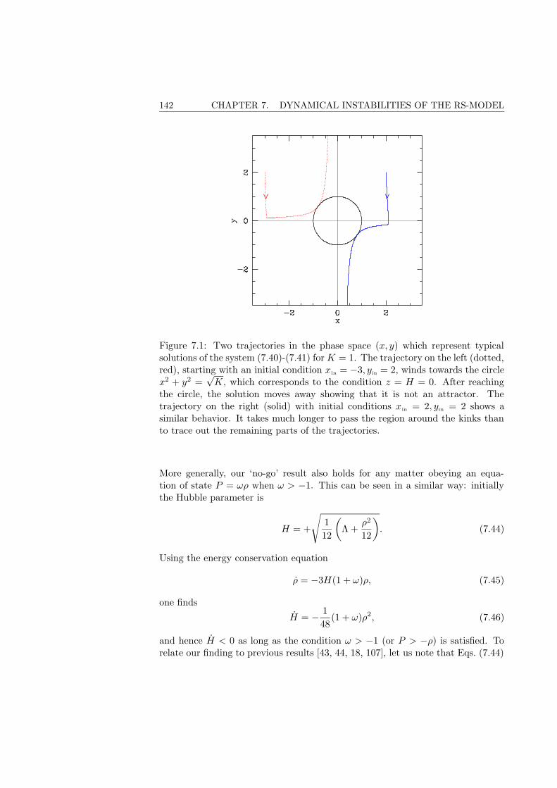
142 CHAPTER 7. DYNAMICAL INSTABILITIES OF THE RS-MODEL
Figure 7.1: Two trajectories in the phase space (x, y) which represent typicalsolutions of the system (7.40)-(7.41) forK = 1. The trajectory on the left (dotted,red), starting with an initial condition xin = −3, yin = 2, winds towards the circlex2 + y2 =
√K, which corresponds to the condition z = H = 0. After reaching
the circle, the solution moves away showing that it is not an attractor. Thetrajectory on the right (solid) with initial conditions xin = 2, yin = 2 shows asimilar behavior. It takes much longer to pass the region around the kinks thanto trace out the remaining parts of the trajectories.
More generally, our ‘no-go’ result also holds for any matter obeying an equa-tion of state P = ωρ when ω > −1. This can be seen in a similar way: initiallythe Hubble parameter is
H = +
√1
12
(Λ +
ρ2
12
). (7.44)
Using the energy conservation equation
ρ = −3H(1 + ω)ρ, (7.45)
one finds
H = − 1
48(1 + ω)ρ2, (7.46)
and hence H < 0 as long as the condition ω > −1 (or P > −ρ) is satisfied. Torelate our finding to previous results [43, 44, 18, 107], let us note that Eqs. (7.44)
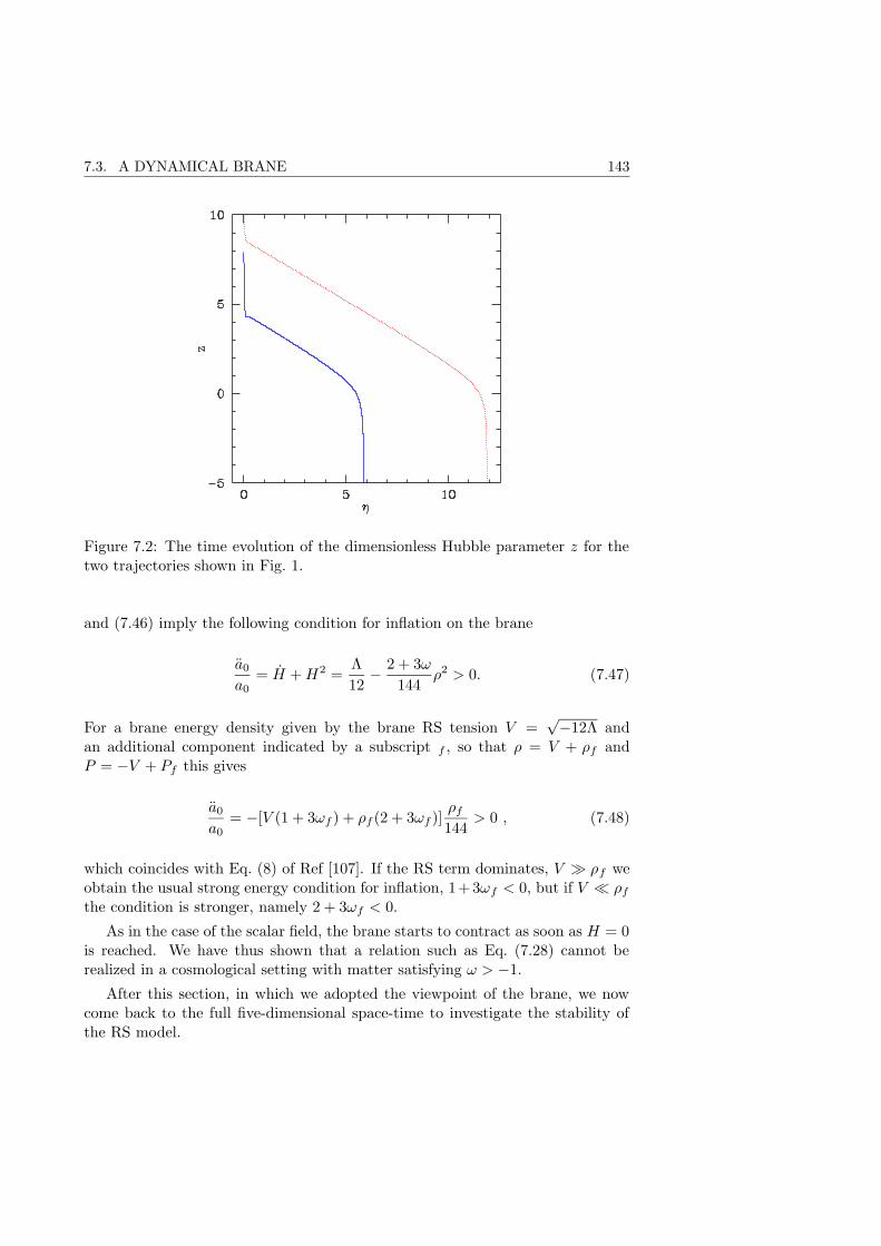
7.3. A DYNAMICAL BRANE 143
Figure 7.2: The time evolution of the dimensionless Hubble parameter z for thetwo trajectories shown in Fig. 1.
and (7.46) imply the following condition for inflation on the brane
a0
a0= H +H2 =
Λ
12− 2 + 3ω
144ρ2 > 0. (7.47)
For a brane energy density given by the brane RS tension V =√−12Λ and
an additional component indicated by a subscript f , so that ρ = V + ρf andP = −V + Pf this gives
a0
a0= −[V (1 + 3ωf ) + ρf (2 + 3ωf )]
ρf
144> 0 , (7.48)
which coincides with Eq. (8) of Ref [107]. If the RS term dominates, V À ρf weobtain the usual strong energy condition for inflation, 1+3ωf < 0, but if V ¿ ρf
the condition is stronger, namely 2 + 3ωf < 0.
As in the case of the scalar field, the brane starts to contract as soon as H = 0is reached. We have thus shown that a relation such as Eq. (7.28) cannot berealized in a cosmological setting with matter satisfying ω > −1.
After this section, in which we adopted the viewpoint of the brane, we nowcome back to the full five-dimensional space-time to investigate the stability ofthe RS model.
144 CHAPTER 7. DYNAMICAL INSTABILITIES OF THE RS-MODEL
7.4 Gauge Invariant Perturbation equations
We formally prove that the five-dimensional RS space-time is unstable under smallhomogeneous perturbations of the brane tension.
7.4.1 Perturbations of the Randall–Sundrum model
The equations of motion derived in Sec. 7.2 provide with N(t, y), R(t, y), andB(t, y) a dynamical generalization of the RS model. We consider Λ and V tobe constant and set the dilaton, the scalar field on the brane and the energy-momentum tensor of the fluid to zero. Equations (7.14)-(7.17) now reduce to
00 : 3e−2N (R2 + RB) + 3e−2B(−R′′ − 2R′2 +R′B′)
− 1
2Λ− δ(y)1
2e−BV = 0 , (7.49)
11 : e−2N (−2R− B − 3R2 − B2 + 2NR+ NB − 2RB)
+ e−2B(N ′′ + 2R′′ +N ′2 + 3R′2 + 2N ′R′ −N ′B′ − 2R′B′)
+1
2Λ + δ(y)
1
2e−BV = 0 , (7.50)
04 : R′ + RR′ −N ′R−R′B = 0 , (7.51)
44 : 3e−2N (−R− 2R2 + NR) + 3e−2B(N ′R′ +R′2) +1
2Λ = 0 .(7.52)
The RS solution (7.27) is a static solution of these equations, provided that condi-tion (7.28) holds. We now derive linear perturbation equations from Eqs. (7.49)-(7.52) which describe the time evolution of small deviations from RS. To this goalwe set
N(t, y) = α|y|+ n(t, y), (7.53)
R(t, y) = α|y|+ r(t, y), (7.54)
B(t, y) = b(t, y), (7.55)
where α = −√
−Λ12 and n(t, y), r(t, y), b(t, y) are small at t = 0. The perturbed
metric isds25 = GMNdxMdxN
= −e2α|y|+2ndt2 + e2α|y|+2rd~x2 + e2bdy2.(7.56)
We consider an energy-momentum tensor deviating from RS only by a slightmismatch of the brane tension
TMN = −ΛGMN − δ(y)δµMδ
νNe−bV gµν , (7.57)
7.4. GAUGE INVARIANT PERTURBATION EQUATIONS 145
withV =
√−12Λ(1 + Ω), (7.58)
where |Ω| ¿ 1 parameterizes the perturbation of the brane tension, GMN is theperturbed metric (7.56) and gµν is its projection onto the brane. Clearly, if alreadythis restricted set of perturbation variables contains an instability, the RS solutionis unstable under homogeneous and isotropic perturbations. Inserting this ansatzinto equations (7.49)– (7.52) and keeping only first order terms, we find
r′′ − 4α2b+ θ(y)α(4r′ − b′)− δ(y)2α(b+ Ω) = 0 , (7.59)
e−2α|y|(2r + b)− n′′ − 2r′′ + 12α2b− θ(y)α(4n′ + 8r′ − 3b′)
+δ(y)6α(b+ Ω) = 0 , (7.60)
r′ − θ(y)αb = 0 , (7.61)
e−2α|y|r + 4α2b− θ(y)α(n′ + 3r′) = 0 , (7.62)
where
θ(y) =
+1 for y > 0−1 for y < 0 .
(7.63)
The junction conditions are
[r′] = [n′] = 2α(b0 + Ω) . (7.64)
Since we want to consider Z2-symmetric perturbations, we require the functionsn, r and b to be symmetric in y. In order to make coordinate-independent state-ments, we rewrite these equations in a gauge invariant way.
7.4.2 Gauge invariant perturbation equations
Under an infinitesimal coordinate transformation induced by the vector field
X = T (t, y)∂t + L(t, y)∂y, (7.65)
the metric perturbations δGMN (corresponding to the first order terms in themetric (7.56)) transform according to
δGMN → δGMN + LXGMN , (7.66)
where LXGMN is the Lie derivative of the static background metric (7.24). Oneobtains the following transformation laws for the variables n, r and b:
n→ n+ θ(y)αL+ T , (7.67)
r → r + θ(y)αL, (7.68)
b→ b+ L′. (7.69)
Since we require the 04 component of the metric to vanish, it must remain zerounder the coordinate transformation. This implies
L = e2α|y|T ′. (7.70)
146 CHAPTER 7. DYNAMICAL INSTABILITIES OF THE RS-MODEL
From Eq. (7.69), together with Z2 symmetry, one finds that L′ must be continuousand symmetric in y. Therefore L must be continuously differentiable and odd iny, which implies L(t, y = 0) = 0. Hence, the perturbation r restricted to the braner0 is gauge invariant. Note that L(t, y = 0) = 0 also follows from Eq. (7.68) andL ∈ C1. Hence the gauge invariance of r0 is not a consequence of Z2 symmetry,but is also preserved for non Z2-symmetric perturbations. By computing the Liederivative of the background energy-momentum tensor from Eq. (7.57) one findsthat the perturbation of the brane tension Ω is gauge invariant. Condition (7.70)and the symmetry property of L′ ensure that there is no energy flow onto or offthe brane. With the following set of gauge invariant quantities
Φ ≡ r′ − θ(y)αb , (7.71)
Ψ ≡ n′ − θ(y)αb− θ(y) 1
αe−2α|y|r , (7.72)
r0 ≡ r(t, y = 0) , (7.73)
Ω, (7.74)
we can rewrite the perturbation equations (7.59)–(7.62) in terms of these variables
Φ′ + θ(y)4αΦ− δ(y)2αΩ = 0 , (7.75)
Ψ′ + 2Φ′ + θ(y)4α(Ψ + 2Φ) + δ(y)
(2
αr0 − 6αΩ
)= 0 , (7.76)
Φ = 0 , (7.77)
Ψ + 3Φ = 0 . (7.78)
The junction conditions are
[Φ] = 2αΩ , [Ψ] = 2αΩ− 2
αr0 . (7.79)
The solutions of equations (7.75) with (7.77) and (7.78) are given by
Φ(y) = −1
3Ψ(y) = θ(y)αΩe−4α|y| + Φ0e
−4α|y| . (7.80)
Z2 symmetry requires Φ to be odd in y and thus Φ0 = 0. Inserting Eq. (7.78) in(7.76) one obtains
r0 = 4α2Ω (7.81)
and after integrationr0(t) = 2α2Ωt2 +Qt, (7.82)
where Q is a small but arbitrary integration constant determined by the initialconditions. (An additive constant to r0 can be absorbed in a redefinition of thespatial coordinates on the brane.) The scale factor on the brane is
e2r0(t) ' 1 + 2r0(t) = 1 + 4α2Ωt2 + 2Qt. (7.83)
7.4. GAUGE INVARIANT PERTURBATION EQUATIONS 147
We have thus found a dynamical instability, which is quadratic in time, when thebrane tension and the bulk cosmological constant are not fine–tuned. Our state-ment is valid in every coordinate system as r0 is gauge invariant. In addition,more surprisingly, in linear perturbation theory there is no constraint on Q, andit cannot be gauged away. This linear instability remains even for Ω = 0, that isif the brane tension is not perturbed at all.
Let us finally discuss our solutions in two particular gauges. As a first gaugecondition we set r′ = 0, which fixes L′ = −θ(y) 1
αr′. The integration constant
on L is determined by the condition L(t, y = 0) = 0. (Note that r′ contains a θfunction and therefore L′ is continuous.) For all values of y we have
r(t) = 2α2Ωt2 +Qt. (7.84)
Since b(y) = −θ(y) 1αΦ(y),
b(y) = −Ωe−4α|y|. (7.85)
From the definition of Ψ it follows that
n′ = −3Φ + θ(y)αb+ θ(y)1
αe−2α|y|r0 , (7.86)
which can be integrated to give
n(t, y) = Ωe−4α|y| − 2Ωe−2α|y| +N (t) . (7.87)
These n, r, and b solve Eqs. (7.59)–(7.62). The integration constant N (t) can beabsorbed in the gauge transformation T . Together with the choice of L′, this fixesthe gauge, and the solutions are therefore unique up to an additive purely timedependent function to T .
Another possible gauge is b = 0. Then, from r′ = Φ,
r(t, y) = −Ω
4e−4α|y| +R(t), (7.88)
with
R(t) = r0(t) +Ω
4= 2α2Ωt2 +Qt+
Ω
4(7.89)
and
n(t, y) =3
4Ωe−4α|y| − 2Ωe−2α|y| +N (t) . (7.90)
Again, the integration constant N (t) can be gauged away by choosing an appro-priate T , and the solutions are uniquely determined by the gauge fixing.
Inserting these solutions in the perturbed metric
ds25 = −e2α|y|+2ndt2 + e2α|y|+2rd~x2 + e2bdy2, (7.91)
148 CHAPTER 7. DYNAMICAL INSTABILITIES OF THE RS-MODEL
we find that the full RS space-time, not only the brane, is unstable against ho-mogeneous perturbations of the brane tension.
We must require the initial perturbations to be small, that is at some initialtime t = 0, the deviation from RS has to be small for all values of y. In the caseof a compact space-time |y| ≤ ymax, this just requires |Ω| ¿ e−4αymax (rememberthat α is a negative constant). For a noncompact space-time −∞ < y < ∞, wehave to require Ω = 0. In other words, for V 6≡
√−12Λ there exists no solution
which is ‘close’ to RS in the sense of L2 or supy at any given initial time.
Finally, we present a geometrical interpretation of the gauge invariant quanti-ties Φ and Ψ. Since the five–dimensional Weyl tensor of the RS solution vanishes,the perturbed Weyl tensor is gauge invariant according to the Steward-Walkerlemma [146]. The 0404 component of the Weyl tensor of the perturbed metric(7.56) is up to first order
C0404 =1
2e2α|y|(n′′ − r′′ + θ(y)α(n′ − r′)) +
1
2(r − b), (7.92)
which can be expressed in terms of gauge invariant quantities
C0404 = −1
2eα|y|
(eα|y|(Φ−Ψ)
)′+ δ(y)
1
αr0. (7.93)
All other nonvanishing Weyl components are multiples of C0404:
C0101 = C0202 = C0303 = C1212 = C1313 = C2323 = −1
3e2α|y|C0404 (7.94)
and
C1414 = C2424 = C3434 =1
3C0404 . (7.95)
In first order the projected Weyl tensor (defined in Ref. [142]) is E11 = E22 =E33 = 1
3E00 = 2α2Ω with Eµµ = 0. The Weyl–tensor completely vanishes for
Ω = 0.
7.5 Results and Conclusions
In this paper we have addressed two main questions: First, we investigatedwhether the RS fine–tuning condition can be obtained dynamically by some mat-ter component on the brane. As a concrete example, we studied a scalar field onthe brane and found that a bulk cosmological constant cannot be cancelled bythe potential of the scalar field in a nontrivial way. This result can be generalizedfor any matter with an equation of state ω > −1.
Second, we studied the stability of the RS model in five dimensions. We havefound that the RS solution is unstable under homogeneous and isotropic, buttime dependent perturbations. For a small deviation of the fine–tuning conditionparameterized by Ω 6= 0, this instability was expected. It is very reminiscent of
7.5. RESULTS AND CONCLUSIONS 149
the instability of the static Einstein universe, where the fluid energy density andthe cosmological constant have to satisfy a delicate balance in order to keep theuniverse static. But even if Ω = 0, there exists a mode (Q 6= 0), which representsan instability in first order perturbation theory. It is interesting to note, that thismode can be absorbed into a motion of the brane, where Q represents the velocityof the brane. In a cosmological context, our result means that a possible changein the brane tension, e.g. during a phase transition, or also quantum correctionsto the bulk energy density (see Ref. [61]) could give rise to instabilities of the fullfive–dimensional space-time. For related work see Refs. [91], [86], [121].
Even if one would consider a dynamical scalar field in the bulk (which doesnot couple to brane fields), which settles into a vacuum state such that its energydensity is constant along the fifth dimension, one would not be able to solve thecosmological constant problem without falling back to some fine–tuning mecha-nism. From our results we can conclude that in order to have a chance to solvethe RS fine tuning problem dynamically, we have to consider fully dynamical bulkfields. This can in principle be done with the system of equations, which we havepresented in Sec. 7.2, and which also applies to the effective five–dimensionallow–energy theory suggested by heterotic M theory [104].
Acknowledgments
We wish to thank Arthur Hebecker, Kerstin Kunze, Marius Mantoiu DanieleSteer, Toby Wiseman and Peter Wittwer for useful discussions and comments.C.v.d.B thanks Geneva university for hospitality. This work was supported bythe Swiss National Science Foundation. C.v.d.B was supported by the DeutscheForschungsgemeinschaft (DFG).

Chapter 8
On CMB anisotropies in abrane universe
152 CHAPTER 8. ON CMB ANISOTROPIES IN A BRANE UNIVERSE
8.1 Introduction
A great deal of our knowledge in cosmology comes from measurements of thecosmic microwave background (CMB), in particular its anisotropies. Recent ex-periments have provided us with precision data which can be used to constrainthe space of cosmological parameters, and thus to confirm or reject cosmologicalmodels. From a theoretical point of view, this is possible because perturbationtheory in a (3+1)-dimensional universe is very well established.
Of course, one would also like to test brane world models with the CMB, inparticular, whether the idea of extra-dimensions is viable at all. Brane worldmodels should leave distinct imprints in the CMB, such that they can hopefullybe strongly constrained in the future. Unfortunately, perturbation theory withextra-dimensions is far more complicated than in the standard (3+1)-dimensionalcase. We have seen in Chap. 6, that the induced Einstein equations (6.37) onthe brane are not a closed system. Therefore, we cannot simply perturb thoseequations, since we miss information on perturbations from the bulk. Instead,we have to perturb the 5-dimensional Einstein equations, which contain the fulldynamics of gravity. The brane is then taken into account via Israel’s junctionconditions.
Recently, a number of works on 5-dimensional perturbation theory have ap-peared (see [129] and references therein). In these treatments the brane is fixed atsome value of the extra-dimensional coordinate, and the bulk is dynamical. Whenone tries to actually solve the corresponding perturbation equations, it turns outthat it is much simpler to consider a static bulk (AdS5 ) and a moving brane.Technically, this is due to the fact that if already the background equations aredynamical, the perturbation equations become extremely cumbersome. In thiscontext, one should note that Israel’s junction conditions do also apply if thebrane is moving.
In this chapter and in the article ‘CMB anisotropies from vector perturbationsin the bulk’ in Chap. 9, we focus on vector perturbations, leaving scalar and tensormodes for future studies. The vector perturbations in the bulk induce vectorperturbations on the brane. In the standard cosmology, vector perturbationsare known to decay for any initial conditions. We shall see in Chap. 9 thatthis is completely different for brane worlds, and therefore the study of vectorperturbations is very interesting.
The second reason to consider vector perturbations is that massless vectormodes in the bulk always remain massless, because they are protected by a gaugesymmetry. Therefore, they should be observable at any (in particular low energy)scale. And finally it is fair to say that vector modes are simpler to treat thanscalars, since they involve only three instead of seven differential equations.
Compared to the mirage cosmology approach, some progress has been made inthat, perturbing Einstein’s equations, the back-reaction is now taken into account.Unfortunately, a direct comparison between the two approaches is not possible,as the perturbation on the probe brane was a scalar describing the fluctuations
8.2. BULK VECTOR PERTURBATIONS IN 4 + 1 DIMENSIONS 153
of its embedding.The outline of this chapter is as follows: in Sec. 8.2 we perturb an AdS5 bulk
and derive the perturbed vector Einstein equations. In the remaining sections,we place ourselves on the brane and recall, how temperature fluctuations in theCMB arise as a result of perturbed photon trajectories (Sec. 8.3), the definitionand some properties of the power spectrum (Sec. 8.4), and finally, how the C`’sare actually calculated from the metric and matter perturbations (Sec. 8.5). Thetreatment in the last three sections is the same as in 4-dimensional standardcosmology.
8.2 Bulk vector perturbations in 4 + 1 dimensions
8.2.1 Background variables
As mentioned in the introduction, the background is taken to be 5-dimensionalanti-de Sitter space-time (AdS5 ). We begin by recalling the relevant backgroundtensors. For the AdS5 metric, we shall use the parametrization given in Eq. (3.63),
ds25 = GMNdxMdxN
=r2
L2(−dt2 + δijdx
idxj) +L2
r2dr2,
(8.1)
where r is the coordinate of the extra-dimension, and L is the curvature radiusof the AdS5 . The Christoffel symbols are calculated using the formula (1.50),
Γµν4 =
1
rδµν , Γ4
µν = − r3
L4ηµν , Γ4
44 = −1
r, (8.2)
where µ = 0, 1, 2, 3, and the other components are zero. Since AdS5 is a space-time of constant negative curvature, we can use the expression for the Ricci tensorand the Riemann scalar from Sec. 2.4,
RMN = − 4
L2GMN , R = − 20
L2. (8.3)
Throughout this and the next chapter, we assume that the bulk is empty, i.e. thatthere is no other form of energy than a (negative) cosmological constant Λ. Then,the 5-dimensional Einstein equations are
0 = GMN + ΛGMN = RMN −1
2GMNR+ ΛGMN =
6
L2GMN + ΛGMN , (8.4)
thus forcing Λ = −6/L2.
8.2.2 Perturbed metric and gauge invariant variables
The splitting of a general 5-dimensional perturbation into scalar, vector, andtensor parts is performed with respect to a 3-dimensional subspaceM3, because
154 CHAPTER 8. ON CMB ANISOTROPIES IN A BRANE UNIVERSE
then the results are directly comparable to the (3+1)-dimensional cosmology. Thescalar, vector, and tensor modes are irreducible components under SO(3) × E3,which is the group of isometries of the unperturbed space time. Here, SO(3)and E3 are the groups of spatial rotations and translations, respectively, andthe terms ‘scalar’, ‘vector’, and ‘tensor’ correspond to the spin-0, spin-1, andspin-2 representations. The advantage of this decomposition is that, in linearperturbation theory, scalar, vector, and tensor modes evolve independently. Inthe following, for the reasons mentioned in the introduction, we restrict ourselvesto vector modes.
In a 5-dimensional space-time there are three vector variables, Bi, Ci, and Ei
needed to parameterize a general vector perturbation,
ds25 = GMNdxMdxN = (GMN + δGMN)dxMdxN
=r2
L2
[−dt2 + 2Bidtdx
i + (δij +∇iEj +∇jEi)dxidxj
]+ 2Cidx
idr +L2
r2dr2,
(8.5)where ∇i denotes the connection inM3. Since Bi, Ci, and Ei are divergenceless1
3-vectors, each of them has only two independent components, and we can seti = 1, 2 for a mode with wave vector k = (0, 0, k). For a more detailed treatment,as well as for the counting of the degrees of freedom, we refer to [129].
Alternatively, we can write Eq. (8.5) in matrix form,
(δGMN) =r2
L2
0 B1 B2 B3 0
B1 H11 H12 H13L2
r2 C1
B2 H12 H22 H23L2
r2 C2
B3 H13 H23 H33L2
r2 C3
0 L2
r2 C1L2
r2 C2L2
r2 C3 0
, (8.6)
with Hij ≡ ∇iEj +∇jEi.
In order to make coordinate independent statements, the perturbed metric iswritten in terms of gauge invariant variables. Under an infinitesimal coordinatetransformation, induced by the divergenceless vector εM ,
xM → xM + εM , εM = (0, εi, 0), (8.7)
with εi = δijεj , the metric perturbations transform as
δGMN → δGMN + LεGMN , (8.8)
where LεGMN is the Lie derivative of the unperturbed metric in the direction εM .
1The divergence term yields a scalar.
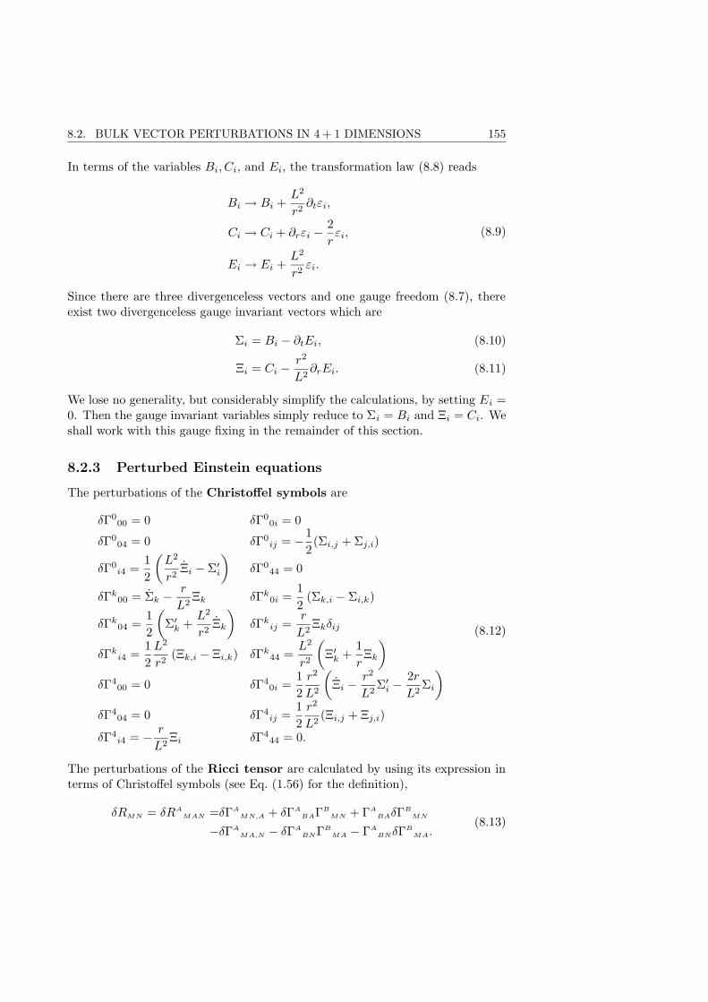
8.2. BULK VECTOR PERTURBATIONS IN 4 + 1 DIMENSIONS 155
In terms of the variables Bi, Ci, and Ei, the transformation law (8.8) reads
Bi → Bi +L2
r2∂tεi,
Ci → Ci + ∂rεi −2
rεi,
Ei → Ei +L2
r2εi.
(8.9)
Since there are three divergenceless vectors and one gauge freedom (8.7), thereexist two divergenceless gauge invariant vectors which are
Σi = Bi − ∂tEi, (8.10)
Ξi = Ci −r2
L2∂rEi. (8.11)
We lose no generality, but considerably simplify the calculations, by setting Ei =0. Then the gauge invariant variables simply reduce to Σi = Bi and Ξi = Ci. Weshall work with this gauge fixing in the remainder of this section.
8.2.3 Perturbed Einstein equations
The perturbations of the Christoffel symbols are
δΓ000 = 0 δΓ0
0i = 0
δΓ004 = 0 δΓ0
ij = −1
2(Σi,j + Σj,i)
δΓ0i4 =
1
2
(L2
r2Ξi − Σ′
i
)δΓ0
44 = 0
δΓk00 = Σk −
r
L2Ξk δΓk
0i =1
2(Σk,i − Σi,k)
δΓk04 =
1
2
(Σ′
k +L2
r2Ξk
)δΓk
ij =r
L2Ξkδij
δΓki4 =
1
2
L2
r2(Ξk,i − Ξi,k) δΓk
44 =L2
r2
(Ξ′
k +1
rΞk
)
δΓ400 = 0 δΓ4
0i =1
2
r2
L2
(Ξi −
r2
L2Σ′
i −2r
L2Σi
)
δΓ404 = 0 δΓ4
ij =1
2
r2
L2(Ξi,j + Ξj,i)
δΓ4i4 = − r
L2Ξi δΓ4
44 = 0.
(8.12)
The perturbations of the Ricci tensor are calculated by using its expression interms of Christoffel symbols (see Eq. (1.56) for the definition),
δRMN = δRAMAN =δΓA
MN,A + δΓABAΓB
MN + ΓABAδΓ
BMN
−δΓAMA,N − δΓA
BNΓBMA − ΓA
BNδΓB
MA.(8.13)
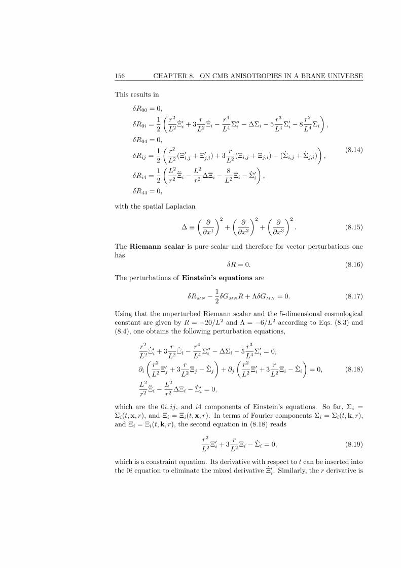
156 CHAPTER 8. ON CMB ANISOTROPIES IN A BRANE UNIVERSE
This results in
δR00 = 0,
δR0i =1
2
(r2
L2Ξ′
i + 3r
L2Ξi −
r4
L4Σ′′
i −∆Σi − 5r3
L4Σ′
i − 8r2
L4Σi
),
δR04 = 0,
δRij =1
2
(r2
L2(Ξ′
i,j + Ξ′j,i) + 3
r
L2(Ξi,j + Ξj,i)− (Σi,j + Σj,i)
),
δRi4 =1
2
(L2
r2Ξi −
L2
r2∆Ξi −
8
L2Ξi − Σ′
i
),
δR44 = 0,
(8.14)
with the spatial Laplacian
∆ ≡(
∂
∂x1
)2
+
(∂
∂x2
)2
+
(∂
∂x3
)2
. (8.15)
The Riemann scalar is pure scalar and therefore for vector perturbations onehas
δR = 0. (8.16)
The perturbations of Einstein’s equations are
δRMN −1
2δGMNR+ ΛδGMN = 0. (8.17)
Using that the unperturbed Riemann scalar and the 5-dimensional cosmologicalconstant are given by R = −20/L2 and Λ = −6/L2 according to Eqs. (8.3) and(8.4), one obtains the following perturbation equations,
r2
L2Ξ′
i + 3r
L2Ξi −
r4
L4Σ′′
i −∆Σi − 5r3
L4Σ′
i = 0,
∂i
(r2
L2Ξ′
j + 3r
L2Ξj − Σj
)+ ∂j
(r2
L2Ξ′
i + 3r
L2Ξi − Σi
)= 0,
L2
r2Ξi −
L2
r2∆Ξi − Σ′
i = 0,
(8.18)
which are the 0i, ij, and i4 components of Einstein’s equations. So far, Σi =Σi(t,x, r), and Ξi = Ξi(t,x, r). In terms of Fourier components Σi = Σi(t,k, r),and Ξi = Ξi(t,k, r), the second equation in (8.18) reads
r2
L2Ξ′
i + 3r
L2Ξi − Σi = 0, (8.19)
which is a constraint equation. Its derivative with respect to t can be inserted intothe 0i equation to eliminate the mixed derivative Ξ′
i. Similarly, the r derivative is
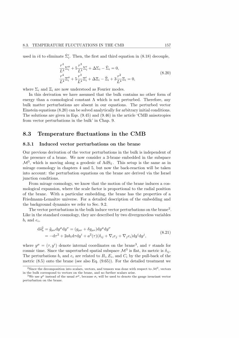
8.3. TEMPERATURE FLUCTUATIONS IN THE CMB 157
used in i4 to eliminate Σ′i. Then, the first and third equation in (8.18) decouple,
r4
L4Σ′′
i + 5r3
L4Σ′
i + ∆Σi − Σi = 0,
r4
L4Ξ′′
i + 5r3
L4Ξ′
i + ∆Ξi − Ξi + 3r2
L4Ξi = 0,
(8.20)
where Σi and Ξi are now understood as Fourier modes.
In this derivation we have assumed that the bulk contains no other form ofenergy than a cosmological constant Λ which is not perturbed. Therefore, anybulk matter perturbations are absent in our equations. The perturbed vectorEinstein equations (8.20) can be solved analytically for arbitrary initial conditions.The solutions are given in Eqs. (9.45) and (9.46) in the article ‘CMB anisotropiesfrom vector perturbations in the bulk’ in Chap. 9.
8.3 Temperature fluctuations in the CMB
8.3.1 Induced vector perturbations on the brane
Our previous derivation of the vector perturbations in the bulk is independent ofthe presence of a brane. We now consider a 3-brane embedded in the subspaceM3, which is moving along a geodesic of AdS5 . This setup is the same as inmirage cosmology in chapters 4 and 5, but now the back-reaction will be takeninto account: the perturbation equations on the brane are derived via the Israeljunction conditions.
From mirage cosmology, we know that the motion of the brane induces a cos-mological expansion, where the scale factor is proportional to the radial positionof the brane. With a particular embedding, the brane has the properties of aFriedmann-Lemaıtre universe. For a detailed description of the embedding andthe background dynamics we refer to Sec. 9.2.
The vector perturbations in the bulk induce vector perturbations on the brane2.Like in the standard cosmology, they are described by two divergenceless variablesbi and ei,
ds2b = gµνdyµdyν = (gµν + δgµν)dyµdyν
= −dτ2 + 2abidτdyi + a2(τ)(δij +∇iej +∇jei)dy
idyj ,(8.21)
where yµ = (τ, yi) denote internal coordinates on the brane3, and τ stands forcosmic time. Since the unperturbed spatial subspaceM3 is flat, its metric is δij .The perturbations bi and ei are related to Bi, Ei, and Ci by the pull-back of themetric (8.5) onto the brane (see also Eq. (9.65)). For the detailed treatment we
2Since the decomposition into scalars, vectors, and tensors was done with respect to M3, vectorsin the bulk correspond to vectors on the brane, and no further scalars arise.
3We use yµ instead of the usual σµ, because σi will be used to denote the gauge invariant vectorperturbation on the brane.
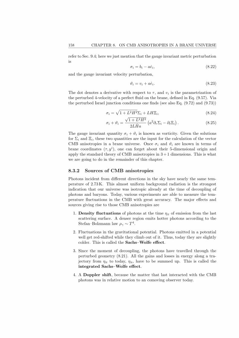
158 CHAPTER 8. ON CMB ANISOTROPIES IN A BRANE UNIVERSE
refer to Sec. 9.4; here we just mention that the gauge invariant metric perturbationis
σi = bi − aei, (8.22)
and the gauge invariant velocity perturbation,
ϑi = vi + aei. (8.23)
The dot denotes a derivative with respect to τ , and vi is the parametrization ofthe perturbed 4-velocity of a perfect fluid on the brane, defined in Eq. (9.57). Viathe perturbed Israel junction conditions one finds (see also Eq. (9.72) and (9.73))
σi =√
1 + L2H2Σi + LHΞi, (8.24)
σi + ϑi =
√1 + L2H2
2LHa
(a2∂rΣi − ∂tΞi
). (8.25)
The gauge invariant quantity σi + ϑi is known as vorticity. Given the solutionsfor Σi and Ξi, these two quantities are the input for the calculation of the vectorCMB anisotropies in a brane universe. Once σi and ϑi are known in terms ofbrane coordinates (τ, yi), one can forget about their 5-dimensional origin andapply the standard theory of CMB anisotropies in 3+1 dimensions. This is whatwe are going to do in the remainder of this chapter.
8.3.2 Sources of CMB anisotropies
Photons incident from different directions in the sky have nearly the same tem-perature of 2.73 K. This almost uniform background radiation is the strongestindication that our universe was isotropic already at the time of decoupling ofphotons and baryons. Today, various experiments are able to measure the tem-perature fluctuations in the CMB with great accuracy. The major effects andsources giving rise to those CMB anisotropies are
1. Density fluctuations of photons at the time ηE of emission from the lastscattering surface. A denser region emits hotter photons according to theStefan–Bolzmann law ργ ∼ T 4.
2. Fluctuations in the gravitational potential. Photons emitted in a potentialwell get red-shifted while they climb out of it. Thus, today they are slightlycolder. This is called the Sachs–Wolfe effect.
3. Since the moment of decoupling, the photons have travelled through theperturbed geometry (8.21). All the gains and losses in energy along a tra-jectory from ηE to today, ηR, have to be summed up. This is called theintegrated Sachs–Wolfe effect.
4. A Doppler shift, because the matter that last interacted with the CMBphotons was in relative motion to an comoving observer today.
8.3. TEMPERATURE FLUCTUATIONS IN THE CMB 159
Further sources of CMB anisotropies can be found e.g. in Ref. [154]. The first twoeffects are associated with perturbations of scalar quantities such as the photondensity contrast. Therefore, we do not take them into account here. The lasttwo effects involve also vector perturbations, and so they are important for ourcalculation of the CMB anisotropies in brane worlds later on. One has to keepin mind that in our treatment the vector perturbations are created in the bulk.When projected onto the brane, they manifest themselves in the same way as thesources listed above. We neglect any vector perturbation that have their originon the brane itself.
The power spectrum that we are going to calculate in the article in Chap. 9looks very different from the standard one, as physics in the extra-dimension leavea distinct imprint in the CMB. We can use this to strongly constrain at least acertain class of brane world models with the CMB.
In the following two paragraphs, we investigate in detail the temperaturefluctuations associated with the integrated Sachs–Wolfe effect.
8.3.3 Temperature fluctuations as a function of the perturba-tion variables
Consider a 4-dimensional Lorentzian manifoldM4 with internal coordinates yµ =(η,y), η denoting conformal time, and a perturbed metric gµν = ηµν + hµν . Wewant to investigate the trajectory of a photon through M4, starting at emissionon the last scattering surface and ending in a telescope today. In parametric form,this trajectory can be written as yµ(λ) = (η(λ),y(λ)), where λ denotes an affineparameter. The perturbed 4-momentum of the photon is
kµ =dyµ
dλ. (8.26)
The unperturbed 4-momentum is parameterized as
kµ = (ν,−νn), (8.27)
where n = (n1, n2, n3) is the direction of observation. Since kµ is a light-like4-vector (ηµνk
µkν = 0), n must be normalized: n2 = 1. The perturbed photonmomentum is parameterized as
kµ = kµ + δkµ = (ν,−νn) + (δk0, δk). (8.28)
We shall see later on, that δk0 has a vector component arising from the metricperturbation σi. We also need to specify the 4-velocity of an observer comovingwith the baryon fluid,
uµ = uµ + δuµ =
(1
a,0
)+(0,vi
a
), (8.29)
uµ = uµ + δuµ = (−a,0) + (0, a(vi + bi)) . (8.30)
160 CHAPTER 8. ON CMB ANISOTROPIES IN A BRANE UNIVERSE
The scale factor a shows up in these expressions, since we have used conformaltime4. Furthermore, we define TR = T (ηR,n) to be the temperature of photonsobserved today in the direction n, and TE = T (ηE,xE) to be the temperature atthe emission point (ηE,xE) on the last scattering surface. The ratio of the twotemperatures is given by
TR
TE
=(kµuµ)R
(kµuµ)E
. (8.31)
From Eqs. (8.28) and (8.30), one finds
kµuµ = −aν(
1 + ni(vi + bi) +1
νδk0
). (8.32)
The combination vi + bi is equal to ϑi + σi according to Eqs. (8.22) and (8.23)and therefore gauge invariant. The denominator in Eq. (8.31) is Taylor expandedin the perturbed quantities such that Eq. (8.31) becomes, up to first order,
TR
TE
=aR
aE
νR
νE
(1 + ni(ϑi + σi)
∣∣RE
+1
νδk0
∣∣∣∣R
E
). (8.33)
The T ∼ 1/a form of the unperturbed temperature curve is recovered by5 settingν ∼ 1/a2. Since the last scattering surface is not a surface of constant time, but asurface of constant free electron density, we make the following expansions aroundthe mean time of emission, ηE,
ηE = ηE + δηE,
aE ≡ a(ηE) = a(ηE) + a′(ηE)δηE ≡ a(ηE) (1 +H(ηE)) δηE,
TE ≡ T (ηE,xE) = T (ηE) + T ′(ηE,xE)δηE ≡ T (ηE) + δTE(ηE,xE),
TR ≡ T (ηR,n) = T (ηR) + T ′(ηR,xR)δηR ≡ T (ηR) + δTR(ηR,n).
(8.34)
Here, the prime denotes a derivative with respect to conformal time η. Thetemperature T (ηE) ≡ TE is a spatial average over the last scattering surface inthe sense of an ensemble average, whereas T (ηR) ≡ TR represents an average overall directions of observations in a unique measurement. Under the assumption ofergodicity, the two ways of averaging are equivalent. From (8.34) one derives
TR
TE
=TR
TE
(1 +
δTR
TR
− δTE
TE
). (8.35)
The left hand side of Eq. (8.33) is now replaced by Eq. (8.35). Isolating δTR/TR
in the resulting expression and using
a(ηE)
aR
=TR
TE
(8.36)
4As a physical quantity, the four-velocity is defined as uµ =dyµ
dτ=
dyµ
dη
dη
dτ=
dyµ
dη
1
a.
5corresponding to the affine parametrizationdη
dλ∼ 1
a2.
8.3. TEMPERATURE FLUCTUATIONS IN THE CMB 161
leads toδTR
TR
= ni(ϑi + σi)∣∣R
E+
1
νδk0
∣∣∣∣R
E
+δTE
TE
+H(ηE)δηE. (8.37)
The left hand side depends only on the direction of observation n and the timeof observation ηR, the right hand side depends on the point of emission and thegeometry along which the photon travels to us. The term δTE/TE in Eq. (8.37)has to be evaluated at (ηE,xE). Using the definition of δTE in Eqs. (8.34) andthe relation (8.36) one finds
δTE
TE
(ηE,xE) =δTE
TE
(ηE,xE)−H(ηE)δηE, (8.38)
such that in Eq. (8.37) the term in H is cancelled. The remaining term can bewritten as
δTE
TE
(ηE,xE) =1
4
δργ
ργ(8.39)
according to the Stephan–Boltzmann law ργ ∼ T 4. This term is a scalar andtherefore we do not consider it in our treatment. With these steps Eq. (8.37)becomes
δTR
TR
= ni(ϑi + σi)∣∣R
E+
1
νδk0
∣∣∣∣R
E
. (8.40)
8.3.4 The perturbed geodesic equation
We are left with the calculation of the term δk0/ν. When a photon travels throughthe perturbed geometry on M4, its 4-momentum is continuously deflected. In-stantaneously, this is measured by the quantity δkµ, which is found by solvingthe perturbed geodesic equation. The calculation can be considerably simplifiedby noting that two conformally equivalent metrics, ds2 = a2ds2, have the samelight-like geodesics. We therefore need only consider the perturbed metric,
ds2 = (ηµν + hµν)dyµdyν = −dη2 +2bidηdyi +(δij +∇iej +∇jei)dy
idyj . (8.41)
The perturbed ‘normalized’ 4-momentum of the photon is then
ˆkµ =
dyµ
dλ, (8.42)
where λ denotes an affine parameter, and the hat indicates that a quantity isassociated with the metric (8.41). We shall use the parameterization
ˆkµ = kµ + δkµ = (1, ki) + (δk0, δki), (8.43)
with the light-like normalization (ki)2 = 1.The perturbed geodesic equation reads
dˆkµ
dλ+ ˆΓµ
αβˆkαˆkβ = 0. (8.44)
162 CHAPTER 8. ON CMB ANISOTROPIES IN A BRANE UNIVERSE
Since the background is time-independent, the unperturbed Christoffel symbolsvanish, and the first order perturbation of the geodesic equation is simply
d
dλδkµ + δΓµ
αβ kαkβ = 0, (8.45)
with
δΓµαβ =
1
2ηµν(hνα,β + hνβ,α − hαβ,ν). (8.46)
Using that hνα,β kβ = d
dλhνα and that, from the unperturbed geodesic equation,
dkµ
dλ= 0, one can integrate Eq. (8.45) from the moment of emission to the moment
of reception. This results in
δkµ∣∣∣
E
R
= −ηµν hναkα∣∣∣
E
R
+1
2ηµν
∫ E
R
dλ hαβ,ν kαkβ . (8.47)
Without loss of generality, we may now choose hij ≡ ∇iej + ∇jei = 0. Then
h0i ≡ bi = σi. Furthermore, h00 = 0 as we are considering only vectors. Uponinserting this into Eq. (8.47), one finds for the zero component
δk0∣∣∣
E
R
= σiki∣∣∣
E
R
−∫ E
R
dλ (∂ησi)ki. (8.48)
Comparing with Eq. (8.27), we make the identifications kµ = (1,−ni) and λ = η.Then δk0 = δk0/ν. Inserting the result (8.48) into (8.40), one finds the finalresult
δTR
TR
= niϑi
∣∣RE
+
∫ R
E
dη (∂ησi)ni. (8.49)
The first term on the right hand side is the perturbation in the Doppler shiftdue to the relative motion of the observer and the emitter. The second term isthe integrated Sachs–Wolfe (ISW) effect: the changes of the geometry perturba-tion along the trajectory, ∂ησi, are projected onto the ‘line of sight’ ni, and theresulting corrections are summed up.
Sometimes it is useful to write the result (8.49) in an alternative form. Tothat end the total derivative along the trajectory is written as
d
dησi(η,y(η)) = ∂ησi +
∂σi
∂yj
∂yj
∂η= ∂ησi − (∂jσi)n
j . (8.50)
Upon partial integration, Eq. (8.49) becomes
δTR
TR
= ni(ϑi + σi)∣∣R
E+
∫ R
E
dη (∂jσi)njni. (8.51)
This form makes the vorticity appear explicitly.Eqs. (8.49) and (8.51) are the final results for the temperature fluctuations in
the CMB in the direction n due to vector perturbations in the standard universeor in a brane world. Notice, that δTR/TR is written entirely in terms of gaugeinvariant variables, as it must be the case for a measurable quantity.
8.4. OBSERVATION OF THE TEMPERATURE FLUCTUATIONS 163
8.4 Observation of the temperature fluctuations
In practice, measurements of the temperature fluctuations in the CMB are ex-pressed in terms of the angular power spectrum C`, where ` is the multipolenumber. In this section, we explore the link between δTR/TR and C`, followingRefs. [154], [152], and [53]. Our mathematical conventions are those of Ref. [70].From the angular power spectrum a variety of cosmological parameters can beextracted.
The temperature fluctuations can be expanded into spherical harmonics Y m` ,
which form a complete set on the 2-sphere:
δTR
TR
≡ δT
T(n, ηR,xR) =
∞∑
`=0
m=∑
m=−`
a`m(ηR,xR)Y m` (n), (8.52)
where the coefficients a`m are given by
a`m(ηR,xR) =
∫
S2
dΩδT
T(n, ηR,xR)Y m
` (n)∗. (8.53)
Here, TR ≡ T = 2.728 ± 0.002 K denotes the mean temperature of the CMB. Inthe following, we are omitting the arguments ηR and xR, which indicate the timeof observation and the position of the observer.
The degree to which the temperature of photons incident from −n and −n′ iscorrelated, is measured by the two point function
⟨δT
T(n)
δT
T(n′)
⟩. (8.54)
The symbol 〈〉 denotes the hypothetical average over an ensemble of universes,i.e. the sum over of all possible different realizations of the CMB for constantcos θ = n · n′. From the definition (8.52) one finds
⟨δT
T(n)
δT
T(n′)
⟩=∑
`,`′
∑
m,m′
〈a`ma`′m′〉Y m` (n)Y m
` (n′)∗, (8.55)
where,
〈a`ma`′m′〉 =∫
dΩ
∫dΩ′
⟨δT
T(n)
δT
T(n′)
⟩Y m
` (n)∗Y m′
`′ (n′). (8.56)
The coefficients a`m originate from a stochastic process, e.g. quantum fluctuationsor phase transitions, that generates perturbations in the early universe. Assumingthat this process is statistically homogeneous and isotropic, one can write
〈a`ma`′m′〉 = δ``′δmm′C`, (8.57)
164 CHAPTER 8. ON CMB ANISOTROPIES IN A BRANE UNIVERSE
where the quantity C` does not depend on xR (homogeneity) or m (isotropy).The C`’s are the CMB power spectrum. Using Eq. (8.57), we obtain
⟨δT
T(n)
δT
T(n′)
⟩=∑
`
C`
∑
m
Y m` (n)Y m
` (n′)∗
︸ ︷︷ ︸= 2`+1
4π P`(n·n′)
=1
4π
∑
`
(2`+ 1)C`P`(n · n′),
(8.58)where we have used the addition theorem for spherical harmoincs, and the P`’sare Legendre’s polynomials. In a spatially flat universe, the index ` is related tothe angle θ between two points on the sky in the directions n and n′ by6
θ =180
`. (8.59)
Thus the quantity (2` + 1)C` appearing in Eq. (8.58) is the amplitude of thetemperature correlation on the angular scale θ. The CMB power spectrum has itshighest peak at ` ' 220, which means that the strongest temperature correlationis between points at an angular distance θ = 180
220 ' 0.8.The relation (8.58) can be inverted to give C` as a function of the temperature
correlator. Multiplying both sides with P`′(µ) (where µ = n ·n′), integrating over
the interval [−1, 1], and using the orthogonality relation∫ 1
−1dµP`(µ)P`′(µ) =
22`+1δ``′ , one finds
C` = 2π
∫ 1
−1
dµ
⟨δT
T(n)
δT
T(n′)
⟩P`(µ). (8.60)
In this ‘hypothetical’ treatment δT/T, a`m, and C` are random variables inan ensemble of universes. Since in practice we cannot reproduce our universemany times, one makes the ergodic hypothesis, that the ensemble average can bereplaced by a spatial average. For a given multipole `, there are 2`+1 independentnumbers a`m over which this average can be taken. One thus defines an estimatorfor the observed CMB power spectrum by
Cobs` ≡ 1
2`+ 1
∑
m=−`
|aobs`m |2. (8.61)
The aobs`m are assumed to be gaussian random variables following a χ2 distribution
with 2` + 1 degrees of freedom. Then the expectation value of Cobs` is equal to
the hypothetical value C`, and the variance is
√(Cobs
` )2 − C2`
C`=
√2
2`+ 1. (8.62)
6This conversion is similar to that between real space and Fourier space quantities, e.g. λ = 2π/k.
8.5. THE C`’S OF VECTOR PERTURBATIONS 165
For large `, the estimator defined in (8.61) is good, whereas for small ` (largescales) the variance is a fundamental limitation on the precision of the measure-ments. This is called ‘cosmic variance’ and is due to the fact that we can observeonly a single realization of the CMB and this only from one given position.
Since in linear perturbation theory scalar, vector, and tensor perturbationsare independent, also the corresponding a`m’s and C`’s are independent
〈aS
`maV
`′m′〉 = 〈aS
`maT
`′m′〉 = 〈aV
`maT
`′m′〉 = 0. (8.63)
8.5 The C`’s of vector perturbations
With the definitions from the previous section, we can now calculate the angularpower spectrum C` for vector perturbations ϑi and σi. The basic idea is to insertexpression (8.49) for δT/T into the correlator 〈a`ma`′m′〉 given in Eq. (8.56), andcarry out the integrals over the sphere. In detail, the procedure is as follows.First, δT/T is expanded into vector Fourier modes,
ϑi(η,x) =1
(2π)3/2
∫d3k ϑi(η,k)eik·x,
σ′i(η,x) =
1
(2π)3/2
∫d3k σ′
i(η,k)eik·x,(8.64)
which allows us to treat each k independently. For a fixed k, one defines a set oforthogonal basis vectors (k, e+, e×) as shown in Fig. 8.1 by
eλ · k = 0, eλ · eλ′
= δλλ′ , λ, λ′ = +,×. (8.65)
Since a photon is transversely polarized, the amplitudes ϑi(η,k) and σ′i(η,k) can
be decomposed into
ϑi(η,k) =∑
λ=+,×ϑλ(η, k)aλ(k)eλ
i (k),
σ′i(η,k) =
∑
λ=+,×σ′
λ(η, k)aλ(k)eλi (k),
(8.66)
where aλ(k) are random amplitudes for each mode k, and eλi are the components
of eλ.
We start our calculation from Eq. (8.49),
δT
T(n) = −niϑi(ηE,xE) +
∫ R
E
dη (∂ησi)ni. (8.67)
The term ϑi(ηR,xR), which is a dipole corresponding to the observers (our) mo-tion, has been omitted since it can be set to zero by a redefinition of the coordi-
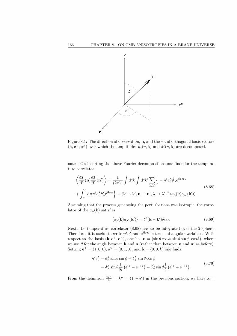
166 CHAPTER 8. ON CMB ANISOTROPIES IN A BRANE UNIVERSE
Figure 8.1: The direction of observation, n, and the set of orthogonal basis vectors(k, e+, e×) over which the amplitudes ϑi(η,k) and σ′
i(η,k) are decomposed.
nates. On inserting the above Fourier decompositions one finds for the tempera-ture correlator,
⟨δT
T(n)
δT
T(n′)
⟩=
1
(2π)3
∫d3k
∫d3k′
∑
λ,λ′
− nieλ
i ϑλeik·xE
+
∫ R
E
dη nieλi σ
′λeik·x
× k→ k′,n→ n′, λ→ λ′∗ 〈aλ(k)aλ′(k′)〉 .
(8.68)
Assuming that the process generating the perturbations was isotropic, the corre-lator of the aλ(k) satisfies
〈aλ(k)aλ′(k′)〉 = δ3(k− k′)δλλ′ . (8.69)
Next, the temperature correlator (8.68) has to be integrated over the 2-sphere.Therefore, it is useful to write nieλ
i and eik·x in terms of angular variables. Withrespect to the basis (k, e+, e×), one has n = (sin θ cosφ, sin θ sinφ, cos θ), wherewe use θ for the angle between k and n (rather than between n and n′ as before).Setting e+ = (1, 0, 0), e× = (0, 1, 0), and k = (0, 0, k) one finds
nieλi = δλ
× sin θ sinφ+ δλ+ sin θ cosφ
= δλ× sin θ
1
2i
(eiφ − e−iφ
)+ δλ
+ sin θ1
2
(eiφ + e−iφ
).
(8.70)
From the definition dxµ
dη = kµ = (1,−ni) in the previous section, we have x =
8.5. THE C`’S OF VECTOR PERTURBATIONS 167
n(ηR − η), and hence
k · x = k · n(ηR − η) = k(ηR − η) cos θ. (8.71)
Eqs. (8.69), (8.70), and (8.71) are inserted into Eq. (8.68), and the k ′-integral andthe sum over λ′ drop out.
When the temperature correlator is integrated over the sphere (see Eq. (8.56)),the quantity
I±`m(η, k) ≡∫
dΩY m` (n)∗ sin θe±iφeik(ηR−η) cos θ (8.72)
appears. The plane wave eik(ηR−η) cos θ is decomposed into spherical Bessel func-tions and Legendre polynomials,
eik(ηR−η) cos θ =
∞∑
`′=0
i`′
(2`′ + 1)j`′ [k(ηR − η)]P`′(cos θ)
=
∞∑
`′=0
i`′
(2`′ + 1)j`′ [k(ηR − η)]√
4π
2`′ + 1Y 0
`′(n),
(8.73)
such that I±`m becomes
I±`m =∑
`′
i`′√
4π(2`′ + 1)j`′ [k(ηR − η)]∫
dΩY m` (n)∗Y 0
`′(n) sin θe±iφ. (8.74)
To solve the integral on the right, one uses the recursion relations for sphericalharmonics to write
sin θe±iφY 0`′ = ∓
√(`′ + 2)(`′ + 1)
(2`′ + 3)(2`′ + 1)Y ±1
`′+1 ±√
`′(`′ − 1)
(2`′ + 1)(2`′ − 1)Y ±1
`′−1. (8.75)
The remaining integral turns out to be simply the orthogonality relation∫
dΩY m` (n)∗Y 1
`′±1(n) = δ`,`′±1δm,1. (8.76)
Putting everything together, one finds
I±`m = ±δm,±1 i`+1
√4π
2`+ 1
√`(`+ 1) j`+1[k(ηR − η)] + j`−1[k(ηR − η)] ,
(8.77)which can be simplified using the relation
j`+1(x) + j`−1(x) =2`+ 1
xj`(x) (8.78)
to give
I±`m = ±δm,±1 i`+1√
4π(2`+ 1)√`(`+ 1)
j`[k(ηR − η)]k(ηR − η)
. (8.79)
168 CHAPTER 8. ON CMB ANISOTROPIES IN A BRANE UNIVERSE
After this side-calculation we now resume the calculation of the the powerspectrum C`. The temperature correlator (8.68) is inserted into Eq. (8.56) for` = `′ and m = m′. Since all information about the stochastic correlations arecontained in aλ(k), and because of the assumption (8.69), we can replace 〈a`ma`m〉by |a`m|2. Then Eq. (8.56) becomes
〈|a`m|2〉 =1
(2π)3
∫d3k
1
4
∣∣∣iϑ×(I+
`m − I−`m)− ϑ+
(I+
`m + I−`m)
+
∫ R
E
dη[−iσ′
×(I+
`m − I−`m)
+ σ′+
(I+
`m + I−`m)] ∣∣∣
2
.
(8.80)We have carried out the remaining sum over λ to remove δλ
+, δλ× coming from
Eq. (8.70). The amplitudes ϑ×, ϑ+, σ′×, σ
′+ were defined in Eq. (8.66). Notice also
that the curly bracket k→ k′,n→ n′, λ→ λ′∗ in Eq. (8.68) has combined withthe first one to give a norm squared, and the factor 1/4 is due to Eq. (8.70).
From Eq. (8.80), one finds C` by averaging over the 2`+1 possible values of maccording to Eq. (8.61). Thereby, the sum over m cancels with δm,±1 in Eq. (8.77)and one obtains the final expression
C` =2
π`(`+ 1)
∫ ∞
0
dk k2|∆`(k)|2,
∆`(k) = − 1√2
(ϑ+ + iϑ×
) j`[k(ηR − ηE)]
k(ηR − ηE)+
∫ E
R
dη1√2
(σ′
+ + iσ′×) j`[k(ηR − η)]
k(ηR − η),
(8.81)where ϑλ = ϑλ(ηE, k), σ
′λ = σλ(η, k), and the prime denotes a derivative with
respect to η.We give an alternative form for ∆`(k) which might be useful in some cases. It
is obtained by partial integration and using
(`− 1)j`−1
x− (`+ 2)
j`+1
x= j′`+1(x) + j′`−1(x). (8.82)
It reads
∆`(k) = − 1√2
((ϑ+ + σ+) + i(ϑ× + σ×)
) j`[k(ηR − ηE)]
k(ηR − ηE)
+k
2`+ 1
∫ E
R
dη1√2
(σ+ + iσ×)j′`+1[k(ηR − η)] + j′`−1[k(ηR − η)]
.
(8.83)Here, the first term involves the vorticity ϑλ + σλ, and the amplitude σλ appearswithout derivative.
Chapter 9
CMB anisotropies fromvector perturbations in thebulk (article)

170 CHAPTER 9. CMB ANISOTROPIES FROM VECTOR PERTURBATIONS
This chapter consists of the article ‘CMB anisotropies from vector perturba-tions in the bulk’, see Ref. [132].
It is also available under http://lanl.arXiv.org/abs/hep-th/0307100.In this article, the internal coordinates on the brane are denoted by yµ instead
of σµ, in order to avoid confusion with the gauge invariant vector perturbationon the brane, σi.
9.1. INTRODUCTION 171
CMB anisotropies from vector perturbations in thebulk
Christophe Ringeval, Timon Boehm, and Ruth DurrerDepartement de Physique Theorique, Universite de Geneve, 24 quai E. Ansermet, CH–1211 Geneva
4 Switzerland.
The vector perturbations induced on the brane by gravitational waves propa-
gating in the bulk are studied in a cosmological framework. Cosmic expansion
arises from the brane motion in a non compact Z2-symmetric five-dimensional
anti-de Sitter space-time. By solving the vector perturbation equations in the
bulk, for generic initial conditions, we find that they give rise to growing modes
on the brane in the Friedmann-Lemaıtre era. Among these modes, we exhibit
a class of normalizable perturbations, which are exponentially growing with re-
spect to conformal time on the brane. The presence of these modes is strongly
constrained by the current observations of the cosmic microwave background
(CMB). We estimate the anisotropies they induce in the CMB, and derive quan-
titative constraints on the allowed amplitude of their primordial spectrum.
PACS number: 04.50.+h, 11.10.Kk, 98.80.Cq
9.1 Introduction
The idea that our universe may have more than three spatial dimensions has beenoriginally introduced by Nordstrom [119], Kaluza [87] and Klein [94]. The factthat superstring theory, the most promising candidate for a theory of quantumgravity, is consistent only in ten space-time dimensions (11 dimensions for Mtheory) has led to a revival of these ideas [124, 125, 77]. It has also been found thatstring theories naturally predict lower dimensional “branes” to which fermions andgauge particles are confined, while gravitons (and the dilaton) propagate in thebulk [8, 126, 105]. Such brane worlds have been studied in a phenomenologicalway already before the discovery that they are actually realized in string theory [3,136].
Recently it has been emphasized that relatively large extra-dimensions (withtypical length L ' µm) can solve the hierarchy problem: the effective four-dimensional and the fundamental D-dimensional Newton constant are related byG4 ∝ GD/L
n. Thus G4 can become very small if the fundamental Planck massis of the order of the electroweak scale. Here n denotes the number of extra-dimensions [12, 13, 9, 128]. It has also been shown that extra-dimensions mayeven be infinite if the geometry contains a so-called “warp factor” [127].
The size of the extra-dimensions is constrained by the requirement of recover-ing usual four-dimensional Einstein gravity on the brane, at least on scales tested
172 CHAPTER 9. CMB ANISOTROPIES FROM VECTOR PERTURBATIONS
by experiments [102, 155, 7]. Models with either a small Planck mass in thebulk [12, 13, 9], or with non compact warped extra-dimensions [128, 127], havebeen shown to lead to an acceptable cosmological phenomenology on the brane [19,44, 43, 142, 60, 107, 135], with or without Z2 symmetry in the bulk [40, 17, 41].Explicit cosmological scenarii leading to a nearly Friedmann-Lemaıtre universe atlate times can be realized on a 3–brane at rest in a dynamical bulk [18, 159] or,alternatively, on a brane moving in an anti-de Sitter bulk [98, 81]. It has beenshown that both approaches are actually equivalent [116].
One can also describe brane worlds as topological defects in the bulk [23,71, 11, 118, 66]. This is equivalent to the geometrical approach in the gravitysector [133], while it admits an explicit mechanism to confine matter and gaugefields on the brane [133, 130, 15, 56, 49, 55, 48, 50, 120, 67, 4, 117]. Dependingon the underlying theory, the stability studies of these defects have shown thatdynamical instabilities may appear on the brane when there are more than onenon compact extra-dimensions [65, 88, 123], whereas this is not the case for a five-dimensional bulk [68], provided that a fine-tuning between the model parametersis fixed [21].
The next step is now to derive observational consequences of brane worldcosmological models, e.g. the anisotropies of the cosmic microwave background(CMB). To that end, a lot of work has recently been invested to derive gauge in-variant perturbation theory in brane worlds with one co-dimension [138, 100, 156,32, 33]. Again, the perturbation equations can be derived when the brane is atrest [129], or when it is moving in a perturbed anti-de Sitter space-time [116, 114,113, 115, 47, 46]. Whatever the approach chosen, the perturbation equations arequite cumbersome and it is difficult to extract interesting physical consequencesanalytically. Also the numerical treatment is much harder than in usual four-dimensional perturbation theory, since it involves partial differential equations.
Nevertheless, it is useful to derive some simple physical consequences of per-turbation theory for brane worlds before performing intensive numerical studies.This has been done for tensor perturbations on the brane in a very phenomenolog-ical way in Ref. [101] or on a more fundamental level in Ref. [62]. Tensor modesin the bulk which induce scalar perturbations on the brane have been studiedin Ref. [54] and it was found that they lead to important constraints for braneworlds.
In this article we consider a brane world in a five-dimensional bulk wherecosmology is induced by the motion of a 3-brane in AdS5 . The bulk perturbationequations are considered without bulk sources and describe gravity waves in thebulk. The present work concentrates on the part of these gravity waves whichresults in vector perturbations on the brane.
For the sake of clarity, we first recall how cosmology on the brane can beobtained via the junction conditions, particularly emphasizing how Z2 symme-try is implemented [19, 44, 43, 142, 60, 107, 135]. After rederiving the bulkperturbation equations for the vector components in terms of gauge invariantvariables [116, 114, 113, 115, 47], we analytically find the most general solutions
9.2. BACKGROUND 173
for arbitrary initial conditions. The time evolution of the induced vector pertur-bations on the brane is then derived using the perturbed junction conditions. Themain result of the paper is that vector perturbations in the bulk generically giverise to vector perturbations on the brane which grow either as a power law oreven exponentially with respect to conformal time. This behavior essentially dif-fers from the usual decay of vector modes in standard four-dimensional cosmology,and may lead to observable effects of extra-dimensions in the CMB.
The outline of the paper is the following: in the next section, the cosmologicalbrane world model obtained by the moving brane in an anti-de Sitter bulk isbriefly recalled. In Sec. 9.3 we set up the vector perturbation equations and solvethem in the bulk. In Sec. 9.4 the induced perturbations on the brane are derivedand compared to those in four-dimensional cosmology, while Sec. 9.5 deals withthe consequences of these new results on CMB anisotropies. The resulting newconstraints for viable brane worlds are discussed in the conclusion.
9.2 Background
As mentioned in the introduction, our universe is considered to be a 3-braneembedded in five-dimensional anti-de Sitter space-time
ds25 = GABdxAdxB =r2
L2
(−dt2 + δijdx
idxj)
+L2
r2dr2. (9.1)
The capital Latin indices A,B run from 0 to 4 and the flat spatial indexes i, jfrom 1 to 3. Anti-de Sitter space-time is a solution of Einstein’s equations with anegative cosmological constant Λ
GAB + ΛGAB = 0, (9.2)
provided that the curvature radius L satisfies
L2 = − 6
Λ. (9.3)
Another coordinate system for anti-de Sitter space can be defined by the co-ordinates transformation r2/L2 = e−2%/L. Then the metric takes the form
ds25 = GABdxAdxB = e−2%/L(−dt2 + δijdx
idxj)
+ d%2, (9.4)
which is often used in brane world models.
9.2.1 Embedding and motion of the brane
The position of the brane in the AdS5 bulk is given by
xM = XM(yµ), (9.5)
174 CHAPTER 9. CMB ANISOTROPIES FROM VECTOR PERTURBATIONS
where XM are embedding functions depending on the internal brane coordinatesyµ (µ = 0, · · · , 3). Using the reparametrization invariance on the brane, we choosexi = Xi = yi. The other embedding functions are written
X0 = tb(τ), X4 = rb(τ), (9.6)
where τ ≡ y0 denotes cosmic time on the brane. Since we want to describe ahomogeneous and isotropic brane, X0 as well asX4 are required to be independentof the spatial coordinates yi. The four tangent vectors to the brane are given by
eM
µ ∂M =∂XM
∂yµ∂M , (9.7)
and the unit space-like normal 1-form nM is defined (up to a sign) by the ortho-gonality and normalization conditions
nMeM
µ = 0, GABnAnB = 1. (9.8)
Adopting the sign convention that n points in the direction in which the brane ismoving (growing rb for an expanding universe), one finds using
e0τ = tb, e4τ = rb, eij = δi
j , (9.9)
the components of the normal
n0 = −rb, n4 = tb, ni = 0. (9.10)
The other components are vanishing, and the dot denotes differentiation withrespect to the brane time τ .
This embedding ensures that the induced metric on the brane describes aspatially flat homogeneous and isotropic universe,
ds2b = gµνdyµdyν = −dτ2 + a2(τ)δijdyidyj , (9.11)
where a(τ) is the usual scale factor, and gµν is the pull-back of the bulk metriconto the brane
gµν = GABeA
µeB
ν , (9.12)
(see e.g. [38, 131]). The first fundamental form qAB is now defined by
qAB = gµνeA
µeB
ν , (9.13)
i.e. the push-forward of the inverse of the induced metric tensor [39, 38]. Onecan also define an orthogonal projector onto the brane which can be expressed interms of the normal 1-form
⊥AB= nAnB = GAB − qAB, (9.14)
in the case of only one codimension.
9.2. BACKGROUND 175
Upon inserting the equations (9.1), (9.10) and (9.13) into the above equation,one finds a parametric form for the brane trajectory [98, 81, 115, 47]
rb(τ) = a(τ)L,
tb(τ) =1
a
√1 + L2H2,
(9.15)
where H = a/a denotes the Hubble parameter on the brane. Alternatively, thisresult can be obtained by comparing expression (9.12) with the Friedmann met-ric (9.11).
Therefore, the unperturbed motion induces a cosmological expansion on the3-brane if rb is growing with tb.
9.2.2 Extrinsic curvature and unperturbed junction conditions
The cosmological evolution on the brane is found by the Lanczos–Sen–Darmois–Israel junction conditions1. They relate the jump of the extrinsic curvature acrossthe brane to its surface energy-momentum content [99, 141, 45, 82]. The extrinsiccurvature tensor projected on the brane can be expressed in terms of the tangentand normal vectors as
kµν = −eA
µeB
ν∇AnB = −1
2eA
µeB
νLnGAB. (9.16)
Here ∇ denotes the covariant derivative with respect to the bulk metric, and Ln
is the five-dimensional Lie-derivative in the direction of the unit normal on thebrane. With the sign choice in Eq. (9.16), the junction conditions read [111]
k>µν − k<
µν = κ25
(Sµν −
1
3S gµν
)≡ κ2
5Sµν , (9.17)
where Sµν is the energy momentum tensor on the brane with trace S, and
κ25 ≡ 6π2G5 =
1
M35
, (9.18)
where M5 and G5 are the five-dimensional (fundamental) Planck mass and New-ton constant, respectively. The superscripts “>” and “<” stand for the bulk sideswith r > rb and r < rb. As already noticed, the brane normal vector nM pointsinto the direction of increasing r [see Eq. (9.10)]. Eq. (9.17) is usually referred toas second junction condition. The first junction condition simply states that thefirst fundamental form (9.13) is continuous across the brane.
In general, there is a force acting on the brane which is due to its curvaturein the higher dimensional geometry. It is given by the contraction of the braneenergy momentum tensor with the average of the extrinsic curvature on both sidesof the brane [17]
Sµν(k>
µν + k<µν
)= 2f. (9.19)
1In the following, they will be simply referred to as “junction conditions”.
176 CHAPTER 9. CMB ANISOTROPIES FROM VECTOR PERTURBATIONS
This force f , normal to the brane, is exerted by the asymmetry of the bulk withrespect to the brane [38, 17]. In this paper, we consider only the case in which thebulk is Z2-symmetric across the brane, hence f = 0. In this case the motion ofthe brane is caused by the stress energy tensor of the brane itself which is exactlythe cosmological situation we have in mind.
From Eqs. (9.10), (9.11), (9.15) and (9.16), noting that the extrinsic curvaturecan be expressed purely in terms of the internal brane coordinates [47, 115], onehas
kµν = −1
2
[GAB
(eA
µ∂νnB + eA
ν ∂µnB)
+ eA
µeB
ν nCGAB,C
]. (9.20)
A short computation shows that the non vanishing components of the extrinsiccurvature tensor are
kττ =1 + L2H2 + `2H
L√
1 + L2H2,
kij = −a2
L
√1 + L2H2δij .
(9.21)
It is clear, that the extrinsic curvature evaluated at some brane position rb doesnot jump if the presence of the brane does not modify anti-de Sitter space. Likein the Randall–Sundrum (RS) model [127], in order to accommodate cosmology,the bulk space-time structure is modified by gluing the mirror symmetric of anti-de Sitter space on one side of the brane onto the other [116]. There are twopossibilities: one can keep the “r > rb” side and replace the “r < rb” side to get
k>µν = kµν , k<
µν = −kµν , (9.22)
where kµν is given by Eq. (9.21). Conversely, keeping the r < rb side leads to
k>µν = −kµν , k<
µν = kµν . (9.23)
Note that both cases verify the force equation (9.19). From the time and spacecomponents of the junction conditions (9.17) one obtains, respectively
±1 + L2H2 + `2H
L√
1 + L2H2=
1
2κ2
5 (P + ρ)− 1
6κ2
5 (ρ+ ρT ) , (9.24)
±√
1 + L2H2
L= −1
6κ2
5 (ρ+ ρT ) . (9.25)
Here the brane stress tensor is assumed to be that of a cosmological fluid plus apure tension ρT , i.e.
Sµν = (P + ρ)uµuν + Pgµν − ρTgµν , (9.26)
ρ and P being the usual energy density and pressure on the brane, and uµ thecomoving four-velocity. The “±” signs in Eqs. (9.24) and (9.25) are obtained bykeeping, respectively, the r > rb, or r < rb, side of the bulk. In order to allow
9.2. BACKGROUND 177
for a positive total brane energy density, ρ+ ρT , we have to keep the r < rb sideand glue it symmetrically on the r > rb one2. In the trivial static (H = 0) casethis construction reproduces the Randall–Sundrum II [127] solution with warpfactor exp(−|%|/L), for −∞ < % < ∞ if we choose rb = L = constant. In ourcoordinates, we just have 0 < r ≤ rb on either side of the brane, and the bulk isnow described by two copies of the “bulk behind the brane”. Even if r only takesvalues inside a finite interval, and even though the volume of the extra dimension,
V = 2
∫ rb
0
√|G| dr =
rb2
(rbL
)3
, (9.27)
is finite, the bulk is semi-compact and its spectrum of perturbation modes has nogap (like in the RS model).
From Eqs. (9.24) and (9.25), one can check that energy conservation on thebrane is verified
ρ+ 3H (P + ρ) = 0. (9.28)
Solving Eq. (9.25) for the Hubble parameter yields
H2 =κ4
5ρT
18ρ
(1 +
ρ
2ρT
)+κ4
5
36ρ2
T −1
L2. (9.29)
At “low energies”, |ρ/ρT | ¿ 1, the usual Friedmann equation is recovered providedthe fine-tuning condition
κ45
36ρ2
T =1
L2(9.30)
is satisfied. The four-dimensional Newton constant is then given by
κ24 ≡ 8πG4 =
κ45ρT
6. (9.31)
Thus a positive tension is required to get a positive effective four-dimensionalNewton constant. Note also that low energy means τ 2 ∼ H−2 À L2. In theFriedmann-Lemaıtre era, the solution of Eq. (9.29) reads
H ' H0
(a
a0
)−3(1+w)/2
,
H ' −3
2(1 + w)H2
0
(a
a0
)−3(1+w)
= −3
2(1 + w)H2,
(9.32)
for a cosmological equation of state P = wρ with constant w. The parametersH0 and a0 refer, respectively, to the Hubble parameter and the scale factor today.For the matter era we have w = 0, and during the radiation era w = 1/3.
2Note that we obtain the same result as in Ref. [47]: a positive brane tension for an expandinguniverse is obtained by keeping the anti-de Sitter side which is “behind the expanding brane withrespect to its motion”.
178 CHAPTER 9. CMB ANISOTROPIES FROM VECTOR PERTURBATIONS
9.3 Gauge invariant perturbation equations in thebulk
A general perturbation in the bulk can be decomposed into “3-scalar”, “3-vector”and “3-tensor” parts which are irreducible components under the group of isome-tries (of the unperturbed space time) SO(3)×E3, the group of three dimensionalrotations and translations. In this paper we restrict ourselves to 3-vector pertur-bations3 and consider an “empty bulk”, i.e. the case where there are no sourcesin the bulk except a negative cosmological constant. With respect to the bulk,and its four spatial dimensions, only bulk gravity waves are therefore consideredsince they are the only modes present when the energy momentum tensor is notperturbed. It is well known (see e.g. Ref. [129]) that gravity waves in 4 + 1 di-mensions have five degrees of freedom which can be decomposed with respect totheir spin in 3 + 1 dimensions into a spin 2 field, the ordinary graviton, a spin1 field, often called the gravi-photon and into a spin 0 field, the gravi-scalar. Inthis work we study the evolution of the gravi-photon in the background describedin the previous section.
After setting up our notations, we find the gauge invariant vector perturbationvariables in the bulk and write down the perturbed Einstein equations. We deriveanalytic solutions for all vector modes in the bulk.
9.3.1 Bulk perturbation variables
Considering only vector perturbations in the bulk, the five dimensional perturbedmetric can be parameterized as
ds25 = − r2
L2dt2 +
r2
L2(δij +∇iEj +∇jEi) dxidxj
+L2
r2dr2 + 2Bi
r2
L2dtdxi + 2Cidx
idr,
(9.33)
where ∇i denotes the connection in the three dimensional subspace of constant tand constant r. Assuming this space to be flat one has ∇i = ∂i. The quantitiesEi, Bi, and Ci are divergenceless vectors i.e. ∂iE
i = ∂iBi = ∂iC
i = 0.
As long as we want to solve for the vector perturbations in the bulk only, thepresence of the brane is not yet relevant. Later it will appear as a boundary con-dition for the bulk perturbations via the junction conditions as will be discussedin paragraph 9.4.3.
Under a linearized vector type coordinate transformation in the bulk, xM →xM + εM , with εM = (0, εi, 0), the perturbation variables defined above transform
3The prefix “3-” will be dropped in what follows, and the term “vector” will be always appliedhere for spin 1 with respect to the surfaces of constant t and r.
9.3. GAUGE INVARIANT PERTURBATION EQUATIONS IN THE BULK 179
as
Ei → Ei +L2
r2εi,
Bi → Bi +L2
r2∂tεi,
Ci → Ci + ∂rεi −2
rεi.
(9.34)
As expected for three divergenceless vector variables and one divergencelessvector type gauge transformation, there remain four degrees of freedom which aredescribed by the two gauge invariant vectors
Σi = Bi − ∂tEi, (9.35)
Ξi = Ci −r2
L2∂rEi. (9.36)
Note that in the gauge Ei = 0 these gauge-invariant variables simply become Bi
and Ci respectively.
9.3.2 Bulk perturbation equations and solutions
A somewhat cumbersome derivation of the Einstein tensor from the metric (9.33)to first order in the perturbations leads to the following vector perturbation equa-tions,
∂tΣ−L
r∂r
(r3
L3Ξ
)= 0, (9.37)
r4
L2∂2
rΣ + 5r3
L2∂rΣ− L2∂2
t Σ + L2∆Σ = 0, (9.38)
r4
L2∂2
r
(r3
L3Ξ
)− r3
L2∂r
(r3
L3Ξ
)− L2∂2
t
(r3
L3Ξ
)+ L2∆
(r3
L3Ξ
)= 0, (9.39)
where ∆ denotes the spatial Laplacian, i.e.
∆ = δij∂i∂j , (9.40)
and the spatial index on Σ and Ξ has been omitted. One can check that theseequations are consistent, e.g. with the master function approach of Ref. [113].
A complete set of solutions for these equations can easily be found by Fouriertransforming with respect to xi, and making the separation ansatz:
Σ(t, r,k) = ΣT(t,k)ΣR(r,k), (9.41)
Ξ(t, r,k) = ΞT(t,k)ΞR(r,k). (9.42)
The most general solution is then a linear combination of such elementary modes.

180 CHAPTER 9. CMB ANISOTROPIES FROM VECTOR PERTURBATIONS
Eq. (9.38) splits into two ordinary differential equations for ΣT and ΣR,
r4∂2
rΣR
ΣR
+ 5r3∂rΣR
ΣR
= ±L4Ω2, (9.43)
∂2t ΣT
ΣT
+ k2 = ±Ω2, (9.44)
where k is the spatial wave number, and ±Ω2 the separation constant having thedimension of an inverse length squared. The frequency Ω represents the rate ofchange of ΣR at r ∼ L, while the rate of change of ΣT is
√|Ω2 ∓ k2|. From the
four-dimensional point of view, −Ω2 can also be interpreted as the mass m2 ofthe mode so that ±Ω2 = −m2. The signs in Eqs. (9.43) and (9.44) come fromthe choice Ω2 ≥ 0. Eq. (9.43) is a Bessel differential equation of order two forthe “−” sign and a modified Bessel equation of order two for the “+” sign [1],while Eq. (9.44) exhibits oscillatory or exponential behavior in bulk time. FromEq. (9.39), similar equations are derived for ΞT(t,k) and ΞR(r,k). This time, theradial function is given by Bessel functions of order one. The constraint equation(9.37) ensures that the separation constant ±Ω2 is the same for both vectors andit also determines their relative amplitude. The general solution of Eqs. (9.37) to(9.39) is a superposition of modes Ω,k which are given by
Σ ∝
L2
r2K2
(L2Ω
r
)e±t
√Ω2 − k2
L2
r2I2
(L2Ω
r
)e±t
√Ω2 − k2
L2
r2J
2
(L2Ω
r
)e±it
√Ω2 + k2
L2
r2Y2
(L2Ω
r
)e±it
√Ω2 + k2
,
(9.45)
Ξ ∝
±√
1− k2/Ω2L2
r2K
1
(L2Ω
r
)e±t
√Ω2 − k2
±√
1− k2/Ω2L2
r2I1
(L2Ω
r
)e±t
√Ω2 − k2
±√
1 + k2/Ω2L2
r2J
1
(L2Ω
r
)ie±it
√Ω2 + k2
±√
1 + k2/Ω2L2
r2Y1
(L2Ω
r
)ie±it
√Ω2 + k2
.
(9.46)
Here Kp and Ip are the modified Bessel functions of order p while Jp and Yp are theordinary ones. The ± signs in Eqs. (9.45) and (9.46) correspond to the two linearlyindependent solutions of Eq. (9.44), whereas the sign of the separation constantdetermines the kind of Bessel functions: +Ω2 (or m2 < 0) for the modified Besselfunction K and I; −Ω2 (or m2 > 0) for the ordinary Bessel functions J and Y. In
9.3. GAUGE INVARIANT PERTURBATION EQUATIONS IN THE BULK 181
general, each of these modes4 can be multiplied by a proportionality coefficientwhich depends on the wave vector k and Ω. Eq. (9.37) ensures that this coefficientis the same for Σ and Ξ. Furthermore, notice that if Ω2 > k2 the K– and I–modes can have an exponentially growing behavior, whereas for Ω2 < k2 one sets√
Ω2 − k2 = i√|Ω2 − k2| such that the modes become oscillatory. The J– and
Y–modes are always oscillating.For a given perturbation mode to be physically acceptable one has to require
that, at some initial time tin, the perturbations are small for all values 0 < r ≤rb(tin), compared to the background. To check that, we use the limiting formsof the Bessel functions [1]. For large arguments, the ordinary Bessel functionsbehave as
Jp(x) ∼
x→∞
√2
πxcos(x− π
2p− π
4
),
Yp(x) ∼
x→∞
√2
πxsin(x− π
2p− π
4
),
(9.47)
while the modified Bessel functions grow or decrease exponentially
Kp(x) ∼
x→∞
√π
2xe−x,
Ip(x) ∼
x→∞1√2πx
ex.
(9.48)
Therefore, in Eqs. (9.45) and (9.46) all modes, except for the K–mode, diverge asr → 0. Hence the only regular modes are
Σ = A(k,Ω)L2
r2K
2
(L2
rΩ
)e±t
√Ω2 − k2
, (9.49)
Ξ = ±A(k,Ω)
√1− k2
Ω2
L2
r2K
1
(L2
rΩ
)e±t
√Ω2 − k2
, (9.50)
where the amplitude A(k,Ω) is determined by the initial conditions and carriesan implicit spatial index. For small wave numbers k2 < Ω2 the growing solutionrapidly dominates, whereas for large wave numbers k2 > Ω2 both solutions arecomparable and oscillating in time. It is easy to see that the K–mode is alsonormalizable in the sense that
∫ rb
0
√|G||Σ|2dr ∝
∫ rb
0
1
r
[K
2
(L2
rΩ
)]2dr <∞,
∫ rb
0
√|G||Ξ|2dr ∝
∫ rb
0
1
r
[K1
(L2
rΩ
)]2dr <∞.
(9.51)
Note that also the J–modes and Y–modes are normalizable. One might viewthis integrability condition as a requirement to insure finiteness of the energy of
4In the following, they will be labeled by the kind of Bessel function they involve, e.g. “K–mode”,“I–mode” etc.
182 CHAPTER 9. CMB ANISOTROPIES FROM VECTOR PERTURBATIONS
these modes. This suggests that the J– and Y–modes could also be excited bysome physical process. Indeed, from Eq. (9.4), their divergence for r → 0 can berecast in terms of the % coordinate, with % → ∞. Expressed in terms of %, theintegrability condition (9.51) ensures that the J– and Y–modes are well definedin the Dirac sense, and thus that a superposition of them may represent physicalperturbations5 [151].
Let us briefly discuss also the zero-mode Ω = 0. The solution of Eqs. (9.37),(9.38) and (9.39) are then
Σ = Ae±ikt, (9.52)
Ξ = ±ikLe±ikt
[A
2
L
r+B
(L
r
)3]. (9.53)
These solutions (which can also be obtained from Eqs. (9.45) and (9.46) in thelimit Ω→ 0) diverge for r → 0 but the A–mode is normalizable in the sense thatthe integrals defined in Eq. (9.51) converge.
Clearly the most intriguing solutions are the K–modes, especially for valuesof the separation constant verifying Ω2 > k2. Then, if present, these fluctuationssoon dominate the others in the bulk. The fact that m2 = −Ω2 < 0 in this caseimplies that the K–modes are tachyonic modes, and it is thus not surprising thatthey may generate instabilities.
Before we go on, let us just note, that all these solutions are also valid solutionsof the bulk vector perturbation equations in the RS model. In their originalwork [127], Randall and Sundrum have obtained very similar equations (we usedsomewhat different variables). However, they considered only the solutions withm2 = +Ω2 > 0 and therefore did not find the growing K–modes. As we shall seein the next section, this choice is justified when one considers boundary conditionswhich do not allow for any anisotropic stresses on the brane. This is indeed wellmotivated as far as cosmology is not concerned. A more detailed discussion ofthe relevance of these modes for the RS model is given in appendix 9.7.1.
In our cosmological framework however, if there is no physical argument whichforbids these modes, they have to be taken seriously since they represent solutionsof the perturbations equations which are small at very early times and growexponentially with respect to bulk time. Note that this instability is linked to theparticular bulk structure considered here where the brane lies at one boundaryof the space-time. In the full AdS5 , 0 < r < ∞, the K–modes are clearly notnormalizable since K
p(L2Ω/r) diverges for r →∞.
At last, one may hope that the K–modes are never generated. However, duringany bulk inflationary phase which leads to the production of 4 + 1 dimensionalgravity waves, as we shall see now, if the anisotropic stresses on the brane donot vanish identically the K–modes are perfectly admissible solutions. For agiven inflationary model, it should be also possible to calculate the spectrum offluctuations, |A(k,Ω)|2.
5This is of course not the case for the I–modes.
9.4. THE INDUCED PERTURBATIONS ON THE BRANE 183
At this stage, the perturbation modes have been only derived in the bulk. Inthe next section, we shall determine the induced perturbations on the brane usingthe perturbed junction conditions.
9.4 The induced perturbations on the brane
9.4.1 Brane perturbation variables
Since we are interested in vector perturbations on the brane induced by those inthe bulk, we parameterize the perturbed induced metric as
ds2b = gµνdyµdyν
= −dτ2 + 2abidτdyi
+ a2 (δij +∇iej +∇jei) dyidyj ,
(9.54)
where ei and bi are divergence free vectors. The junction conditions which relatethe bulk perturbation variables to the perturbations of the brane can be writtenin terms of gauge invariant variables. Under an infinitesimal transformation yµ →yµ + ξµ, where ξµ = (0, a2ξi), we have
ei → ei + ξi,
bi → bi + aξi.(9.55)
Here the dot is the derivative with respect to the brane time τ and ξi is a di-vergence free vector field. Hence the gauge invariant vector perturbation is [52]
σi = bi − aei. (9.56)
This variable fully describes the vector metric perturbations on the brane.The brane energy momentum tensor Sµν given in Eq. (9.26) has also to be
perturbed. As we shall see, the junction conditions (together with Z2 symmetry)do in general require a perturbed energy momentum tensor on the brane. Sincewe only consider vector perturbations δρ = δP = 0. However, the perturbedfour-velocity of the perfect fluid does contain a vector part uµ = uµ + δuµ, with
δuµ =
0vi
a
, (9.57)
and where vi is divergenceless. Under yµ → yµ + ξµ,
vi → vi − aξi, (9.58)
where vi ≡ δijvi. A gauge invariant perturbed velocity can therefore be defined
asϑi = vi + aei. (9.59)
184 CHAPTER 9. CMB ANISOTROPIES FROM VECTOR PERTURBATIONS
In addition, the anisotropic stresses contain a vector component denoted πi. Sincethe corresponding background quantity vanishes, this variable is gauge invariantaccording to the Stewart–Walker lemma [146].
In summary, there are three gauge invariant brane perturbation variables. Weshall use the combinations
σi = bi − aei,
ϑi = vi + aei,
πi.
(9.60)
To apply the junction conditions we need to determine the perturbations ofthe reduced energy momentum tensor defined in Eq. (9.17). In terms of our gaugeinvariant quantities they read
δSττ = 0, (9.61)
δSτi = −a(P +
2
3ρ− 1
3ρT
)σi − a (P + ρ)ϑi, (9.62)
δSij = a2P (∂iπj + ∂jπi) . (9.63)
9.4.2 Perturbed induced metric and extrinsic curvature
We now express the perturbed induced metric, and the perturbed extrinsic cur-vature in terms of the bulk perturbation variables [47]. In principle there are twocontributions to the brane perturbations: perturbations of the bulk geometry aswell as perturbations of the brane position. A bulk perturbed quantity has then tobe evaluated at the perturbed brane position [see Eq. (9.6)]. Using reparametriza-tion invariance on the brane [47], the perturbed embedding can be described interms of a single variable Υ,
XM = XM + ΥnM , (9.64)
where all quantities are functions of the brane coordinates yµ. Since Υ is a scalarperturbation it does not play a role in our treatment, and we can consider onlythe perturbations δGAB due to the perturbed bulk geometry evaluated at theunperturbed brane position. The induced metric perturbation is then given by
δgµν = gµν − gµν = eA
µeB
ν δGAB. (9.65)
From Eqs. (9.33), (9.35), (9.36) and (9.65) one finds in the gauge Ei = 0
δgττ = 0,
δgτi = a√
1 + L2H2Σi + aLHΞi,
δgij = δGij = 0.
(9.66)
The time component vanishes as it is a pure scalar, and the purely spatial compo-nents can be set to zero without loss of generality by gauge fixing (Ei = ei = 0).
9.4. THE INDUCED PERTURBATIONS ON THE BRANE 185
In the same way, perturbing Eq. (9.20), and making use of Eqs. (9.7), (9.8)in order to derive the perturbed normal vector, leads to (again we use the gaugeEi = 0)
δkττ = 0, (9.67)
δkτi =1
2∂tΞi −
1
2a2∂rΣi − aH
√1 + L2H2Ξi
− a
L
(1 + L2H2
)Σi, (9.68)
δkij =1
2aLH (∂iΣj + ∂jΣi)
+1
2a√
1 + L2H2 (∂iΞj + ∂jΞi) , (9.69)
where δkµν = kµν−kµν , and all bulk quantities have to be evaluated at the braneposition. In the derivation we have also used that on the brane ∂µ = eA
µ∂A.
9.4.3 Perturbed junction conditions and solutions
The first junction condition requires the first fundamental form qAB to be conti-nuous across the brane. Therefore, the components of the induced metric (9.54)are given by the explicit expressions (9.66). This leads to the following relations
ei = Ei,
bi =√
1 + L2H2Bi + LHCi,(9.70)
where the bulk quantities have to be evaluated at the brane position (tb, rb). Forσi = bi − aei we use
aei = a(tb∂tEi + rb∂rEi
)
=√
1 + L2H2∂tEi + a2LH∂rEi.(9.71)
Together with Eqs. (9.35) and (9.36) this gives
σi =√
1 + L2H2Σi + LHΞi. (9.72)
The equations corresponding to the second junction condition are obtained byperturbing Eq. (9.17) (using Z2 symmetry, k>
µν = −k<µν = −kµν) and inserting
the expressions (9.68), (9.69) for the perturbed extrinsic curvature tensor, withEqs. (9.62), (9.63) for the perturbed energy-momentum tensor on the brane. Aftersome algebra one obtains for the 0i and the ij components, respectively
2LH√1 + L2H2
a (σi + ϑi) = a2∂rΣi − ∂tΞi, (9.73)
κ25aPπi = −LHΣi −
√1 + L2H2Ξi, (9.74)
186 CHAPTER 9. CMB ANISOTROPIES FROM VECTOR PERTURBATIONS
where we have used the unperturbed junction conditions, Eqs. (9.24) and (9.25),and the fact that on the brane ∂µ = eA
µ∂A.
In the RS model one has H = H = 0 and the requirement that the anisotropicstresses vanish identically. We show in appendix 9.7.1 that the well-known resultsof Refs. [127] and [151] are recovered in this limit.
Hence, if by some mechanism, like e.g. bulk inflation, gravity waves are pro-duced in the bulk, their vector parts Σi and Ξi will induce vector metric perturba-tions σi on the brane according to Eq. (9.72). The vorticity σi+ϑi and anisotropicstresses πi on the brane define boundary conditions for the bulk variables accord-ing to Eqs. (9.73) and (9.74). In general, the time evolution of πi may be givenby some additional matter equation, like e.g. the Boltzmann equation or somedissipation equation which usually depends also on the metric perturbations. Itis interesting to note that for generic initial conditions in the bulk, the amplitudeof the K–mode does not vanish, which means that the anisotropic stresses on thebrane may grow exponentially. At late time (for LH ¿ 1) Eq. (9.74) reduces toκ2
5aPπi = −Ξi. A generally covariant equation of motion for πi must be com-patible with this behavior since it is a simple consequence of the 5-dimensionalEinstein equations for a certain choice of initial conditions.
In the following we do not want to specify a particular mechanism which ge-nerates Σi and Ξi, and just assume they have been produced with some spectrumgiven by A(k,Ω). In usual 4-dimensional cosmology it is well-known that vectorperturbations decay. Therefore, in ordinary 4-dimensional inflationary scenariosthey are not considered. Only if they are continuously re-generated like, e.g. inmodels with topological defects (see e.g. Ref. [51]), vector modes affect CMBanisotropies. Here the situation is different since the modes considered are eitherexponentially growing or oscillating with respect to bulk time. Therefore, weexpect the behavior of vector perturbations to be very different from the usual4-dimensional results even in the absence of K–modes.
In the following, we assume that the boundary and initial conditions are suchthe πi(tin) 6≡ 0. They therefore allow for K–mode contributions. Clearly, if thishappens it leads to exponential growth of σi and πi. However, before concludingabout the viability of these modes, one has to check if they have observableconsequences on the brane. Indeed, anisotropic stresses are often very small(e.g. of second order only) and one may therefore hope that the initial amplitudesof the K–modes are also very small and do not lead to destructives effects, atleast on time scales equal to the age of the universe. By estimating the inducedCMB anisotropies, we show in the next section that this is not the case.
9.5 CMB anisotropies
To calculate the CMB anisotropies from the vector perturbations induced by bulkgravity waves, the relevant quantities are σ and ϑ+ σ given in terms of the bulkvariables by Eqs. (9.72) and (9.73). Inserting the solutions (9.49) and (9.50) for
9.5. CMB ANISOTROPIES 187
the K–mode into (9.72) and (9.73) yields
σ(tb,k) = A(k,Ω)
[√1 + L2H2
1
a2K
2
(LΩ
a
)
± LH√
1− k2
Ω2
1
a2K
1
(LΩ
a
)]e±tb
√Ω2 − k2
,
(9.75)
and
(σ + ϑ) (tb,k) = A(k,Ω)k2
Ω2
√1 + L2H2
2L2H
LΩ
a
1
a2K1
(LΩ
a
)e±tb
√Ω2 − k2
, (9.76)
where again we have omitted the spatial index i on σ, ϑ and A. Similar equationscan be obtained for the J– and Y–modes by replacing, in Eqs. (9.75) and (9.76),the modified Bessel functions by the ordinary ones, plus the transformations:−k2 → k2 and ± → ±i.
These equations are still written in bulk time tb which is related to the con-formal time η on the brane by
dtb =√
1 + L2H2 dη. (9.77)
Therefore, at sufficiently late time L2H2 ¿ 1 such that dtb ' dη. Note that Lis the size of the extra-dimension which must be smaller than micrometers whileH−1 is the Hubble scale which is larger than 105 light years at times later thanrecombination which are of interest for CMB anisotropies.
As a result, the growing or oscillating behavior in bulk time carries over to con-formal time. Moreover there are additional time dependent terms in Eqs. (9.75)and (9.76) with respect to Eqs. (9.49) and (9.50) due to the motion of the brane.As can be seen from Eqs. (9.75) and (9.76), the modes evolve quite differently fordifferent values of their physical bulk wave number Ω/a. In the limit Ω/a¿ 1/Land for Ω2 > k2, the growing K–modes behave like
σ ∼ 2A
(ΩL)2eη
√Ω2−k2
,
σ + ϑ ∼ A
(ΩL)2k2
2a2Heη
√Ω2−k2
,
(9.78)
where use has been made of L2H2 ¿ 1, and of the limiting forms of Besselfunction for small arguments [1]
Kp(x) ∼x→0
1
2Γ(p)
(2
x
)p
. (9.79)
In the same way, from Eq. (9.48), the K–modes verifying Ω/aÀ 1/L reduce to
σ ∼ A
(ΩL)2eη
√Ω2−k2
√π
2
(ΩL
a
)3/2
e−ΩL/a,
σ + ϑ ∼ A
(ΩL)2k2
2a2Heη
√Ω2−k2
√π
2
(ΩL
a
)1/2
e−ΩL/a.
(9.80)
188 CHAPTER 9. CMB ANISOTROPIES FROM VECTOR PERTURBATIONS
They are exponentially damped compared to the former [see Eq. (9.78)]. As aresult, the main contribution of the K–mode vector perturbations comes fromthe modes with a physical wave number Ω/a smaller than the energy scale 1/Lassociated with the extra-dimension. As the universe expands, a mode with fixedvalue Ω remains relatively small as long as the exponents in Eq. (9.80) satisfy
Ω
aL− η
√Ω2 − k2 ' 1
a
(ΩL− τ
√Ω2 − k2
)> 0. (9.81)
When this inequality is violated, for k ¿ Ω this is soon after τ ∼ L, the modestarts growing exponentially. The time τ ∼ L also corresponds to the initial timeat which the evolution of the universe starts to become Friedmannian.
In the same way, one can derive the behavior of the J– and Y–modes on thebrane for physical bulk wave numbers greater or smaller than the size of the extra-dimension. This time, the exponentially growing terms are replaced by oscillatoryones, and the ordinary Bessel functions are approximated by (see Eq. (9.47) andRef. [1])
Jp(x) ∼x→0
1
Γ(p+ 1)
(x2
)p
,
Yp(x) ∼x→0− 1
πΓ(p)
(2
x
)p
.
(9.82)
From Eqs. (9.47) and (9.82), the equivalents of Eqs. (9.75) and (9.76) for J–and Y–modes can be shown to oscillate always. From Eq. (9.32), their amplitudeis found to decay like a−3/2 in the short wavelength limit Ω/a À 1/L. In thelong wavelength limit Ω/a ¿ 1/L, the amplitude of the Y–mode stays constantwhereas the J–mode decreases as a−4.
The vorticity is also found to oscillate in conformal time. This time, theamplitude of the long wavelength Y–modes always grows as a3w+1 while for theJ–modes it behaves like a3w−1. Finally, in the short wavelength limit, both Y andJ vorticity modes grow like a3w+1/2.
Whatever the kind of physical vector perturbation modes excited in the bulk,we have shown that there always exist bulk wave numbers Ω that give rise togrowing vector perturbations on the brane. Although the J– and Y–modes ge-nerate vorticity growing like a power law of the scale factor, they can be, in afirst approximation, neglected compared to the K–modes which grows like an ex-ponential of the conformal time. We therefore now concentrate on the K–modesand derive constraints on their initial amplitude A(k,Ω) by estimating the CMBanisotropies they induce.
In order to determine the temperature fluctuations in the CMB due to vectorperturbations on the brane, we have to calculate how a photon emitted on the lastscattering surface travels through the perturbed geometry (9.54). A receiver to-day (with conformal time ηR) therefore measures different microwave backgroundtemperatures T (ηR, n
i) for incident photons coming from different directions ni.With the conventions and formulae in the paragraphs 8.3.3 and 8.3.4 the vector-
9.5. CMB ANISOTROPIES 189
type temperature fluctuations read
δTR(ni)
TR
= ni (σi + ϑi)|RE +
∫ R
E
∂σi
∂xjninjdλ,
= −niϑi(ηE) +
∫ R
E
σ′in
idη,
(9.83)
where λ denotes the affine parameter along the photon trajectory and the primeis a derivative with respect to conformal time η. The “R” and “E” index referto the time of photon reception (today) and emission at recombination. For thesecond equality we have used
dσi
dλ= σ′
i − nj ∂σi
∂xj, (9.84)
where −ni is the direction of the photon momentum. We have also neglected thecontribution from the upper boundary, “R”, in the first term since it simply givesrise to a dipole term. The first term in Eq. (9.83) is a Doppler shift, and thesecond is known as integrated Sachs-Wolfe effect. To determine the angular CMBpower spectrum C`, we apply the total angular momentum formalism developedby Hu and White [80]. According to this, a vector perturbation v is decomposedas
v = e+v+ + e×v×, (9.85)
where e+,× are defined so that (e+, e×, and k = k/k) form a righthanded or-thonormal system. Using this decomposition for ϑi and σi, one obtains the an-gular CMB perturbation spectrum C` via
C` =2
π`(`+ 1)
∫ ∞
0
k2〈|∆`(k)|2〉dk, (9.86)
where
∆`(k) = −ϑ+(ηE , k)j`(kη0
− kηE)
kη0− kη
E
+
∫ η0
ηE
σ+′(η, k)j`(kη0
− kη)kη0 − kη
dη.(9.87)
In Eq. (9.87) we have assumed that the process which generates the fluctuationshas no preferred handedness so that 〈|σ+|2〉 = 〈|σ×|2〉 as well as 〈|ϑ+|2〉 = 〈|ϑ×|2〉.Omitting the + and × superscripts, we can take into account the other modesimply by a factor 2. Furthermore, we have redefined η
0≡ ηR.
As shown in the previous section, the main contribution of the K–modes comesfrom those having long wavelengths a/ΩÀ L, and k < Ω. In the following, onlythese modes will be considered. Since they are growing exponentially in η, theintegrated Sachs-Wolfe contribution will dominate and we concentrate on it inwhat follows. A more rigorous justification is given in appendix 9.7.2. Inserting
190 CHAPTER 9. CMB ANISOTROPIES FROM VECTOR PERTURBATIONS
the limiting form (9.78) for σ in Eq. (9.87) gives
∆`(k) ' 2A0Ωnkne$
0
√1−k2
√1
k2− 1
×∫ x
E
0
j`(x)
xe−x√
1/k2−1dx,
(9.88)
where a simple power law ansatz has been chosen for the primordial amplitude
√〈|A(k,Ω)|2〉 = A0(Ω)Ω2L2kn. (9.89)
A dimensionless wave number k, and conformal time$, have also been introducedas
k =k
Ω, $ = ηΩ, (9.90)
in order to measure their physical counterparts in units of the bulk wavelengths.The condition k < Ω now becomes k < 1. The integration over η in the inte-grated Sachs-Wolfe term is transformed into an integration over the dimensionlessvariable x defined by
x = k (η0− η) = k ($
0−$) , (9.91)
the subscript “0” refers to the present time. Note that xE = k (η0 − ηE) ' kη0 .By observing the CMB, one may naturally expect that the perturbations with
physical wavelength greater than the horizon size today have almost no effect. Interms of our parameters, this means that the main contribution in the C` comesfrom the modes verifying Ω/a0 > H0 , hence $0 > 1.
In appendix 9.7.2, we derive a crude approximation for the angular powerspectrum induced by the exponentially growing K–modes, in a range a little moreconstrained than the one previously motivated, namely
`maxH0<
Ω
a0
<L−1
1 + zE
, (9.92)
where zE is the redshift at photon emission which is taken to coincide with re-combination, zE ' 103. In order to simplify the calculation, we do not wantthe transition between the damped K–modes (Ω/a > L−1) and the exponentiallygrowing ones (Ω/a < L−1) to occur between the last scattering surface and today.This requirement leads to the upper limit of Eq. (9.92). Moreover, in order to de-rive the C`, we perform an expansion with respect to a parameter `/$0 assumedsmall, and `max refers to the multipole at which this approximation breaks down.The lower limit in Eq. (9.92) comes from this approximation. Using the valuesL ' 10−3 mm, H−1
0' 1029 mm, `max ' 103, and z
E' 103, one finds
10−26 mm−1 <Ω
a0
< 1 mm−1. (9.93)
9.6. CONCLUSION 191
The corresponding allowed range for the parameter $0 becomes [see Eq. (9.116)]
103 < $0 < 1029. (9.94)
Clearly the detailed peak structure on the CMB anisotropy spectrum wouldhave been different if we had taken into account the oscillatory parts (k > Ω) ofthe K–modes, as well as the Y– and J–modes, but here we are only interestedin estimating an order of magnitude bound. As detailed in appendix 9.7.2, for ascale invariant initial spectrum, i.e. n = −3/2, we obtain
`(`+ 1)
2πC` & (A
0e$
0 )2 e−`
`7/2
(`
$0
)`−1
. (9.95)
From current observations of the CMB anisotropies, the left hand side of thisexpression is about 10−10, and for ` ' 10, one gets
A0(Ω) .
e−[$0−5 ln($0 )]
105. (9.96)
From Eq. (9.116) and (9.94), one finds that the primordial amplitude of thesemodes must satisfy
A0(Ω) < e−103
, for Ω/a0' 10−26mm−1 (9.97)
and, more dramatically,
A0(Ω) < e−1029
, for Ω/a0' 1mm−1 (9.98)
for the short wavelength modes. As expected, the perturbations with wavelengthcloser to the horizon today (smaller values of Ω) are less constrained than smallerwavelengths [see Eq. (9.97)]. Moreover, one may expect that the bound (9.98)is no longer valid for Ω/a
0> L−1/(1 + z
E) since the modes in Eq. (9.80) start
to contribute. However, the present results concern more than 20 orders of mag-nitude for the physical bulk wave numbers Ω/a
0, and show that the exhibited
modes are actually very dangerous for the brane world model we are interestedin.
It seems that the only way to avoid these constraints is to find a physicalmechanism forbidding any excitation of these modes.
9.6 Conclusion
In this paper we have shown that vector perturbations in the bulk generically leadto growing vector perturbations on the brane in the Friedmann-Lemaıtre era. Thisbehavior radically differs from the usual one in four-dimensional cosmology, wherevector modes decay like a−2 whatever the initial conditions.
Among the growing modes, we have identified so called K–modes which areperfectly normalizable and lead to exponentially growing vector perturbations on
192 CHAPTER 9. CMB ANISOTROPIES FROM VECTOR PERTURBATIONS
the brane with respect to conformal time. By means of a rough estimate of theCMB anisotropies induced by these perturbations, we have shown that they areseverely incompatible with a homogeneous and isotropic universe; they light upa fire in the microwave sky, unless their primordial amplitude is extremely small.
No particular mechanism for the generation of these modes has been specified.However, one expects that bulk inflation leads to gravitational waves in the bulkwhich do generically contain them. Even if they are not generated directly, theyshould be induced in the bulk by second order effects. Usually, these effects aretoo small to have any physical consequences, but here they would largely sufficedue to the exponential growth of the K–modes [see Eqs. (9.97) and (9.98)]. Thissecond order induction seems very difficult to prevent in the models discussedhere.
It is interesting to note that this result is also linked to the presence of anon compact extra-dimension which allows a continuum of bulk frequencies Ω.A closer examination of Eq. (9.44) shows that the mode Ω = 0, admits only J–and Y–mode behaviors. In a compact space, provided the first quantized valueof Ω is sufficiently large, one could expect the exponentially growing K–modesto be never excited by low energy physical processes. Another more speculativeway to dispose of them could be to consider their causal structure: as we havenoticed before, the modes with separation constant +Ω2 are tachyons of mass−Ω2 from the four-dimensional point of view. From the five-dimensional point ofview, these are not “propagating modes”, but “brane-modes” which decay intothe fifth dimension with penetration depth d = L2Ω.
In a more basic theory, which goes beyond our classical relativistic approach,these modes may thus not be allowed at all.
Finally, we want to retain that even if the K–modes can be eliminated insome way, the growing behavior of the Y– and J–modes remains. Although theirpower law growth is not as critical as the exponential growth of the K–modes,they should have significant effects on the CMB anisotropies. Indeed, they leadto amplified oscillating vector perturbations which are entirely absent in four-dimensional cosmology.
We therefore conclude that, if no physical mechanism forbids the generationof the discussed vector modes with time dependence ∝ exp(η
√Ω2 − k2), anti-
de Sitter infinitly thin brane worlds, with non compact extra-dimension, cannotreasonably lead to a homogeneous and isotropic expanding universe.
Acknowledgments
It is a pleasure to thank Robert Brandenberger, Cedric Deffayet, Roy Maartens,Filippo Vernizzi, David Wands and Peter Wittwer for helpful discussions. Thiswork is supported by the Swiss National Science Foundation. We also acknowledgetechnical and moral support by Martin Zimmermann in the last phase of theproject.
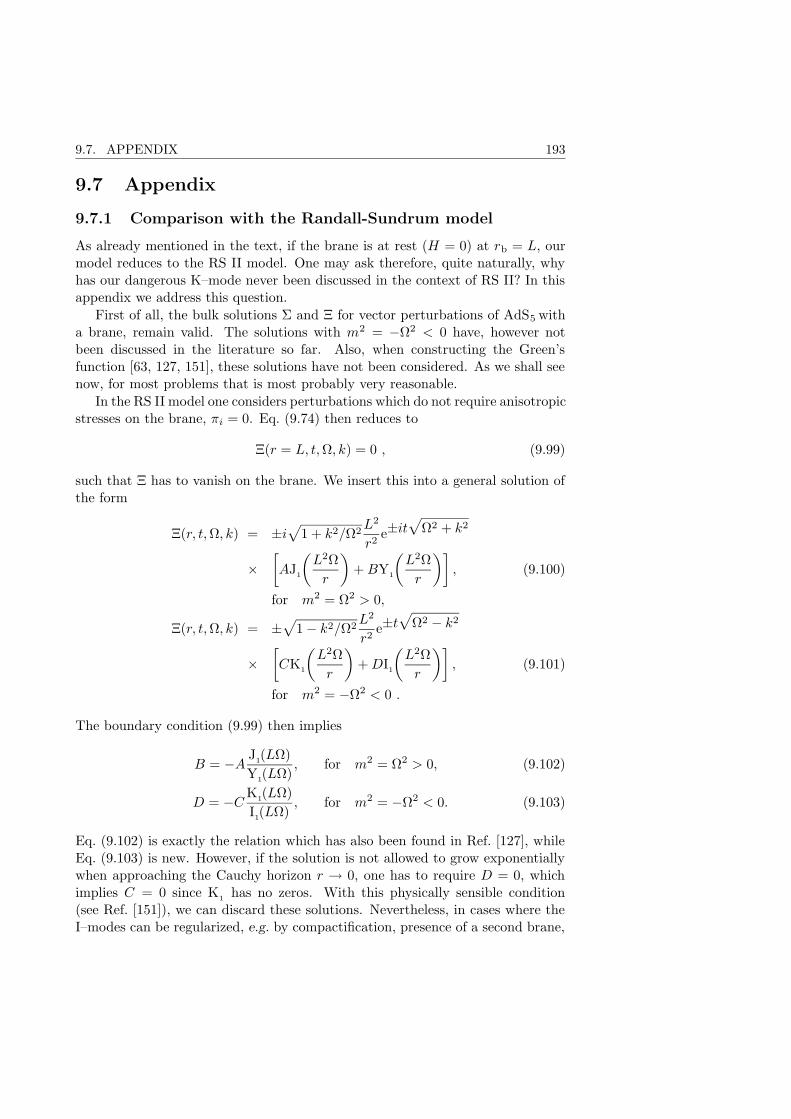
9.7. APPENDIX 193
9.7 Appendix
9.7.1 Comparison with the Randall-Sundrum model
As already mentioned in the text, if the brane is at rest (H = 0) at rb = L, ourmodel reduces to the RS II model. One may ask therefore, quite naturally, whyhas our dangerous K–mode never been discussed in the context of RS II? In thisappendix we address this question.
First of all, the bulk solutions Σ and Ξ for vector perturbations of AdS5 witha brane, remain valid. The solutions with m2 = −Ω2 < 0 have, however notbeen discussed in the literature so far. Also, when constructing the Green’sfunction [63, 127, 151], these solutions have not been considered. As we shall seenow, for most problems that is most probably very reasonable.
In the RS II model one considers perturbations which do not require anisotropicstresses on the brane, πi = 0. Eq. (9.74) then reduces to
Ξ(r = L, t,Ω, k) = 0 , (9.99)
such that Ξ has to vanish on the brane. We insert this into a general solution ofthe form
Ξ(r, t,Ω, k) = ±i√
1 + k2/Ω2L2
r2e±it
√Ω2 + k2
×[AJ
1
(L2Ω
r
)+BY
1
(L2Ω
r
)], (9.100)
for m2 = Ω2 > 0,
Ξ(r, t,Ω, k) = ±√
1− k2/Ω2L2
r2e±t
√Ω2 − k2
×[CK
1
(L2Ω
r
)+DI
1
(L2Ω
r
)], (9.101)
for m2 = −Ω2 < 0 .
The boundary condition (9.99) then implies
B = −A J1(LΩ)
Y1(LΩ), for m2 = Ω2 > 0, (9.102)
D = −CK1(LΩ)
I1(LΩ), for m2 = −Ω2 < 0. (9.103)
Eq. (9.102) is exactly the relation which has also been found in Ref. [127], whileEq. (9.103) is new. However, if the solution is not allowed to grow exponentiallywhen approaching the Cauchy horizon r → 0, one has to require D = 0, whichimplies C = 0 since K1 has no zeros. With this physically sensible condition(see Ref. [151]), we can discard these solutions. Nevertheless, in cases where theI–modes can be regularized, e.g. by compactification, presence of a second brane,
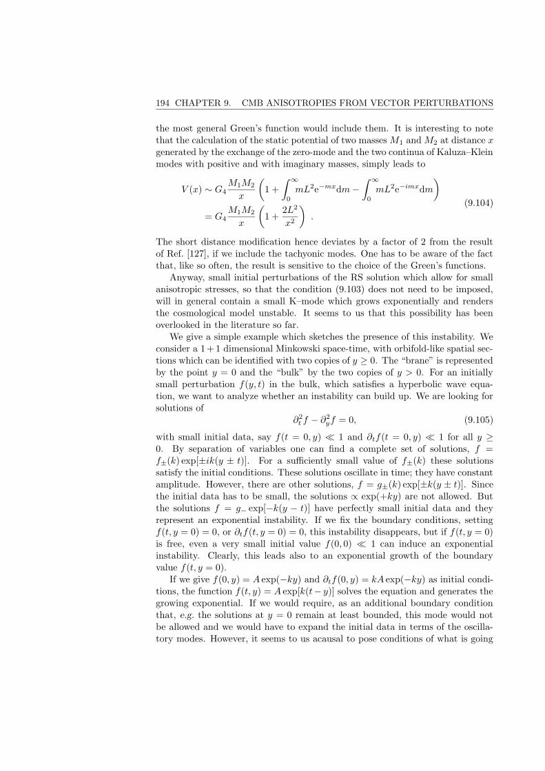
194 CHAPTER 9. CMB ANISOTROPIES FROM VECTOR PERTURBATIONS
the most general Green’s function would include them. It is interesting to notethat the calculation of the static potential of two masses M1 and M2 at distance xgenerated by the exchange of the zero-mode and the two continua of Kaluza–Kleinmodes with positive and with imaginary masses, simply leads to
V (x) ∼ G4M1M2
x
(1 +
∫ ∞
0
mL2e−mxdm−∫ ∞
0
mL2e−imxdm
)
= G4M1M2
x
(1 +
2L2
x2
).
(9.104)
The short distance modification hence deviates by a factor of 2 from the resultof Ref. [127], if we include the tachyonic modes. One has to be aware of the factthat, like so often, the result is sensitive to the choice of the Green’s functions.
Anyway, small initial perturbations of the RS solution which allow for smallanisotropic stresses, so that the condition (9.103) does not need to be imposed,will in general contain a small K–mode which grows exponentially and rendersthe cosmological model unstable. It seems to us that this possibility has beenoverlooked in the literature so far.
We give a simple example which sketches the presence of this instability. Weconsider a 1+1 dimensional Minkowski space-time, with orbifold-like spatial sec-tions which can be identified with two copies of y ≥ 0. The “brane” is representedby the point y = 0 and the “bulk” by the two copies of y > 0. For an initiallysmall perturbation f(y, t) in the bulk, which satisfies a hyperbolic wave equa-tion, we want to analyze whether an instability can build up. We are looking forsolutions of
∂2t f − ∂2
yf = 0, (9.105)
with small initial data, say f(t = 0, y) ¿ 1 and ∂tf(t = 0, y) ¿ 1 for all y ≥0. By separation of variables one can find a complete set of solutions, f =f±(k) exp[±ik(y ± t)]. For a sufficiently small value of f±(k) these solutionssatisfy the initial conditions. These solutions oscillate in time; they have constantamplitude. However, there are other solutions, f = g±(k) exp[±k(y ± t)]. Sincethe initial data has to be small, the solutions ∝ exp(+ky) are not allowed. Butthe solutions f = g− exp[−k(y − t)] have perfectly small initial data and theyrepresent an exponential instability. If we fix the boundary conditions, settingf(t, y = 0) = 0, or ∂tf(t, y = 0) = 0, this instability disappears, but if f(t, y = 0)is free, even a very small initial value f(0, 0) ¿ 1 can induce an exponentialinstability. Clearly, this leads also to an exponential growth of the boundaryvalue f(t, y = 0).
If we give f(0, y) = A exp(−ky) and ∂tf(0, y) = kA exp(−ky) as initial condi-tions, the function f(t, y) = A exp[k(t− y)] solves the equation and generates thegrowing exponential. If we would require, as an additional boundary conditionthat, e.g. the solutions at y = 0 remain at least bounded, this mode would notbe allowed and we would have to expand the initial data in terms of the oscilla-tory modes. However, it seems to us acausal to pose conditions of what is going
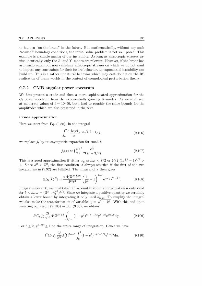
9.7. APPENDIX 195
to happen “on the brane” in the future. But mathematically, without any such“acausal” boundary conditions, the initial value problem is not well posed. Thisexample is a simple analog of our instability. As long as anisotropic stresses va-nish identically, only the J– and Y–modes are relevant. However, if the brane hasarbitrarily small but non vanishing anisotropic stresses on which we do not wantto impose any constraints for their future behavior, an exponential instability canbuild up. This is a rather unnatural behavior which may cast doubts on the RSrealisation of brane worlds in the context of cosmological perturbation theory.
9.7.2 CMB angular power spectrum
We first present a crude and then a more sophisticated approximation for theC` power spectrum from the exponentially growing K–modes. As we shall see,at moderate values of ` ∼ 10–50, both lead to roughly the same bounds for theamplitudes which are also presented in the text.
Crude approximation
Here we start from Eq. (9.88). In the integral∫ x
E
0
j`(x)
xe−x√
1/k2−1dx, (9.106)
we replace j` by its asymptotic expansion for small `,
j`(x) '(x
2
)`√π
2Γ(`+ 3/2). (9.107)
This is a good approximation if either xE ' kη0 < `/2 or (`/2)(1/k2 − 1)1/2 >1. Since k2 < Ω2, the first condition is always satisfied if the first of the twoinequalities in (9.92) are fulfilled. The integral of x then gives
〈|∆`(k)|2〉 'πA2
0Ω2nk2n
22``3
(1
k2− 1
)1−`
e2$0
√1−k2
. (9.108)
Integrating over k, we must take into account that our approximation is only validfor k < kmax = (Ω2− η−2
0 )1/2. Since we integrate a positive quantity we certainlyobtain a lower bound by integrating it only until kmax. To simplify the integral
we also make the transformation of variables y =√
1− k2. With this and uponinserting our result (9.108) in Eq. (9.86), we obtain
`2C` &2`
22`A2
0Ω2n+3
∫ 1
1/$0
(1− y2)n+`−1/2y3−2`e2$0ydy. (9.109)
For ` ≥ 2, y3−2` ≥ 1 on the entire range of integration. Hence we have
`2C` &2`
22`A2
0Ω2n+3
∫ 1
0
(1− y2)n+`−1/2e2$0ydy. (9.110)
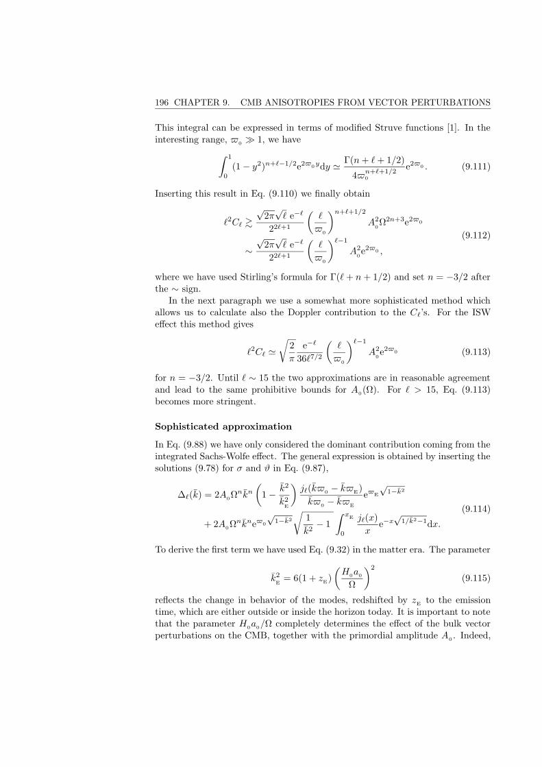
196 CHAPTER 9. CMB ANISOTROPIES FROM VECTOR PERTURBATIONS
This integral can be expressed in terms of modified Struve functions [1]. In theinteresting range, $0 À 1, we have
∫ 1
0
(1− y2)n+`−1/2e2$0ydy ' Γ(n+ `+ 1/2)
4$n+`+1/20
e2$0 . (9.111)
Inserting this result in Eq. (9.110) we finally obtain
`2C` &
√2π√` e−`
22`+1
(`
$0
)n+`+1/2
A20Ω2n+3e2$0
∼√
2π√` e−`
22`+1
(`
$0
)`−1
A20e2$0 ,
(9.112)
where we have used Stirling’s formula for Γ(`+ n+ 1/2) and set n = −3/2 afterthe ∼ sign.
In the next paragraph we use a somewhat more sophisticated method whichallows us to calculate also the Doppler contribution to the C`’s. For the ISWeffect this method gives
`2C` '√
2
π
e−`
36`7/2
(`
$0
)`−1
A20e2$0 (9.113)
for n = −3/2. Until ` ∼ 15 the two approximations are in reasonable agreementand lead to the same prohibitive bounds for A
0(Ω). For ` > 15, Eq. (9.113)
becomes more stringent.
Sophisticated approximation
In Eq. (9.88) we have only considered the dominant contribution coming from theintegrated Sachs-Wolfe effect. The general expression is obtained by inserting thesolutions (9.78) for σ and ϑ in Eq. (9.87),
∆`(k) = 2A0Ωnkn
(1− k2
k2E
)j`(k$0 − k$E)
k$0 − k$E
e$E
√1−k2
+ 2A0Ωnkne$0
√1−k2
√1
k2− 1
∫ xE
0
j`(x)
xe−x√
1/k2−1dx.
(9.114)
To derive the first term we have used Eq. (9.32) in the matter era. The parameter
k2E
= 6(1 + zE)
(H0a0
Ω
)2
(9.115)
reflects the change in behavior of the modes, redshifted by zE to the emissiontime, which are either outside or inside the horizon today. It is important to notethat the parameter H0a0/Ω completely determines the effect of the bulk vectorperturbations on the CMB, together with the primordial amplitude A0 . Indeed,
9.7. APPENDIX 197
solving Eq. (9.29) in terms of conformal time, and using Eqs. (9.28) and (9.32),yields η0 ' 2/(a0H0) in the Friedmann-Lemaıtre era. Thus
$0' 2
Ω/a0
H0
, $E' 1
1 + zE
Ω/a0
H0
. (9.116)
We now replace the spherical Bessel functions j`
in the integrated Sachs-Wolfeterm (ISW) using the relation [1]
j`(x) =
√π
2xJ
`+1/2(x). (9.117)
In the ISW term the upper integration limit can be taken to be infinity as thecontribution from xE to infinity can be neglected provided x
√1/k2 − 1 > 1. This
restriction is equivalent to k2 < 1− 1/$0
which is verified for almost all values ofk up to one, given that $
0varies in the assumed range (9.94). We remind that
for the exponentially growing K–mode k ≤ Ω, and hence 0 ≤ k ≤ 1. This allowsfor the exact solution [70]∫ ∞
0
x−3/2J`+1/2
(x)e−x√
1/k2−1dx =k`
2`+1/2
Γ(`)
Γ(`+ 3/2)F
(`
2,`
2+ 1; `+
3
2; k2
),
(9.118)where F is the Gauss hypergeometric function. In regard to the subsequentintegration over k we approximate F as follows. For small values of k, F is nearlyconstant with value 1, at k = 0. As k → 1 the slope of F diverges and it cannotbe Taylor expanded anymore. However, by means of the linear transformationformulas [1], F can be written as a combination of hypergeometric functionsdepending on 1− k2
F
(`
2,`
2+ 1; `+
3
2; k2
)=
Γ
(`+
3
2
)Γ
(1
2
)
Γ
(`
2+
3
2
)Γ
(`
2+
1
2
)F(`
2,`
2+ 1;
1
2; 1− k2
)
+√
1− k2
Γ
(`+
3
2
)Γ
(−1
2
)
Γ
(`
2
)Γ
(`
2+ 1
) F
(`
2+
3
2,`
2+
1
2;3
2; 1− k2
).
(9.119)These in turn can be expanded around 1− k2 = 0, and gives
F ∼k→1
2`+1/2(1− `
√1− k2
). (9.120)
These two approximations intersect at k =√
1− 1/`2. In this way, we canevaluate the mean value of F by integrating the two parts over the interval [0, 1].Thus, the hypergeometric function is replaced by
F
(`
2,`
2+ 1; `+
3
2; k2
)' 2`+1/2
6`2. (9.121)
198 CHAPTER 9. CMB ANISOTROPIES FROM VECTOR PERTURBATIONS
Furthermore, the Gamma functions in (9.118) can be approximated using Stir-ling’s formula [1]
Γ(`)
Γ(`+ 3/2)' 1
`3/2. (9.122)
Putting everything together and squaring Eq. (9.114) we obtain
|∆`(k)|2 = 2πA20k2nΩ2n
(1− k2
k2E
)2e2$
E
√1−k2
k3($0−$
E)3(J
`+1/2
[k($
0−$
E)])2
+ 2
(1− k2
k2E
)e($0+$
E)√
1−k2
k3/2($0−$
E)3/2
J`+1/2
[k($
0−$
E)] k`−1
√1− k2
6`7/2
+ e2$0
√1−k2 k2(`−1)(1− k2)
36`7
.
(9.123)The C`’s are then found by integrating over all k-modes
C` =2
π`(`+ 1)Ω3
∫ 1
0
k2|∆`(k)|2dk
≡ 4A20`(`+ 1)Ω2n+3
(C
(1)` + C
(2)` + C
(3)`
),
(9.124)
where the C(i)` correspond to the three terms in Eq. (9.123). In the following we
keep only the zero order terms in $0/$E . From Eqs. (9.123), (9.124) one finds
C(1)` =
1
$30
∫ 1
0
k2n−1
(1− k2
k2E
)2
e2$E
√1−k2 [
J`+1/2
(k$0
)]2dk. (9.125)
First, notice that if the argument is larger or smaller than the index, the Besselfunctions are well approximated by their asymptotic expansions (9.47) and (9.82),respectively. Therefore, we split the k-integral into two integrals over the intervals[0, k`] and [k`, 1], in each of which the Bessel function is replaced by its limitingforms. The transition value k` is given by k` ' `/$0 . In the integral from k`
to 1, the sin2(k$0) is then replaced by its mean value 1/2 which is justified ifthe multiplying function varies much slower in k than the sine. To carry out theintegration we make the substitution y2 = 1 − k2, and in order to simplify thenotation we define the integral
I(a, b, ν) =
∫ b
a
y(1− y2)νe2$E
ydy. (9.126)
9.7. APPENDIX 199
In this way we can write Eq. (9.125) in the form
C(1)` =
1
π$40
[I(0, y`, n− 3/2)− 2
k2E
I(0, y`, n− 1/2) +1
k4E
I(0, y`, n+ 1/2)]
+1
Γ2(`+ 3/2)
($0
2
)2`+1 [I(y`, 1, `+ n− 1/2)
− 2
k2E
I(y`, 1, `+ n+ 1/2) +1
k4E
I(y`, 1, `+ n+ 3/2)].
(9.127)
Since y` =√
1− k2` is very close to one, and the integrand is continuous in the
interval [0, 1], integrals of the form I(y`, 1, ν) can be well approximated by themean value
I(y`, 1, ν) ' y(1− y2)νe2$E
y∣∣y=y`
(1− y`) 'e2$
E
2
(`
$0
)2(ν+1)
. (9.128)
For the integrals of the type I(0, y`, ν) we distinguish between three cases:
Case a: ν > −1. This case corresponds to a spectral index n > 1/2 in the firstintegral in Eq. (9.125). We write I(0, y`, ν) = I(0, 1, ν) − I(y`, 1, ν). Thesolution of the latter is given by Eq. (9.128), whereas the former can besolved in terms of modified Bessel and Struve functions [70]
I(0, 1, ν) =1
2(ν + 1)+
√π
2$−1/2−ν
EΓ(ν + 1)
[I
ν+3/2(2$E) + L
ν+3/2(2$E)
].
(9.129)Since our derivation assumes $
E> `, the large argument limit applies and
we have
Iν+3/2
(2$E) + Lν+3/2
(2$E) ' e2$E
√π$
E
, (9.130)
independently of the index ν.
Case b: ν = −1. Since the above expressions, Eq. (9.129), diverge for ν = −1,we approximate the integral by
I(0, y`, ν) ' e2$E
∫ y`
0
y(1− y2)−1dy = −e2$E ln
(`
$0
). (9.131)
We have checked that the numerical solution of I(0, y`, ν) agrees well withthe approximation, provided y` is close to 1.
Case c: ν < −1. We use the same simplification as in Eq. (9.131), and now theintegral yields
I(0, y`, ν) ' e2$E
∫ y`
0
y(1− y2)νdy = − e2$E
2(ν + 1)
(`
$0
)2(ν+1)
. (9.132)
200 CHAPTER 9. CMB ANISOTROPIES FROM VECTOR PERTURBATIONS
For the particular value n = −3/2, Eq. (9.127) contains terms I(0, y`,−3) andI(0, y`,−2) which can be evaluated according to (9.132), and a term I(0, y`,−1)for which we use (9.131). The remaining three integrals over the interval [y`, 1]are evaluated by (9.128). The result is
C(1)` ' e$
0/z
E
4π`4
[1− `2
6zE
−(
`2
12zE
)2
ln
(`
$0
)+
e2β`
2
(1− `2
24zE
)2]. (9.133)
The parameter β is a constant of order unity, within in our approximation it isβ = 1− ln 2 ∼ 0.3.
The second term C(2)` in Eq. (9.123) reads
C(2)` ' 1
3`7/2$3/2s0
∫ 1
0
e($0+$E
)√
1−k2k2n+`−1/2
×√
1− k2
(1− k2
k2E
)J
`+1/2(k$0)dk,
(9.134)
where only the zero order terms in $E/$
0has been kept. Using the limiting
forms for the Bessel function for arguments smaller and larger than the transitionvalue k`, yields
C(2)` ' 1
3`7/2$3/20 Γ(`+ 3/2)
∫ k`
0
e($0+$
E)√
1−k2k2n+`−1/2
×√
1− k2
(1− k2
k2E
)(k$
0
2
)`+1/2
dk
+21/2
3π1/2`7/2$0
∫ 1
k`
e($0+$E
)√
1−k2k2n+`−1
×√
1− k2
(1− k2
k2E
)sin(k$0 −
π
2`)dk.
(9.135)
For consistency with the derivation of C(1)` , we have assumed that the main
contribution comes from the first integral, while the second one is small due tothe oscillating integrand. Since k` ¿ 1, we can use again the mean value formulato evaluate the first integral, and by the Stirling formula for Γ(`+3/2), Eq. (9.135)becomes
C(2)` ' e$
0
12π1/2`11/2
(`
$0
)2n+`+2
eβ`
(1− `2
24zE
). (9.136)
Since ` < $0, the spectrum is damped at large `, while the other terms can lead
to the appearance of a bump, depending on the value of $0
and n.
The last terms C(3)` reads
C(3)` =
1
36`7
∫ 1
0
e2$0
√1−k2
k2n+2`(1− k2
)dk. (9.137)
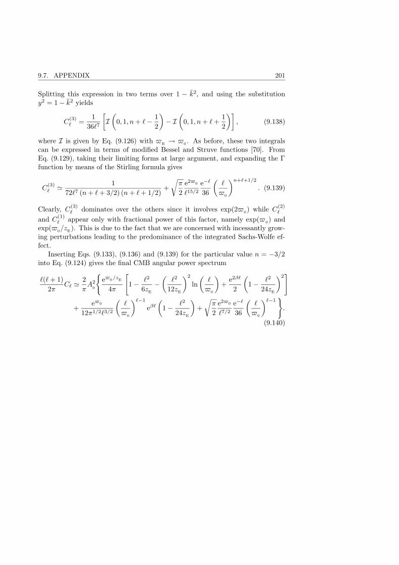
9.7. APPENDIX 201
Splitting this expression in two terms over 1 − k2, and using the substitutiony2 = 1− k2 yields
C(3)` =
1
36`7
[I(
0, 1, n+ `− 1
2
)− I
(0, 1, n+ `+
1
2
)], (9.138)
where I is given by Eq. (9.126) with $E→ $
0. As before, these two integrals
can be expressed in terms of modified Bessel and Struve functions [70]. FromEq. (9.129), taking their limiting forms at large argument, and expanding the Γfunction by means of the Stirling formula gives
C(3)` ' 1
72`7 (n+ `+ 3/2) (n+ `+ 1/2)+
√π
2
e2$0
`15/2
e−`
36
(`
$0
)n+`+1/2
. (9.139)
Clearly, C(3)` dominates over the others since it involves exp(2$
0) while C
(2)`
and C(1)` appear only with fractional power of this factor, namely exp($
0) and
exp($0/z
E). This is due to the fact that we are concerned with incessantly grow-
ing perturbations leading to the predominance of the integrated Sachs-Wolfe ef-fect.
Inserting Eqs. (9.133), (9.136) and (9.139) for the particular value n = −3/2into Eq. (9.124) gives the final CMB angular power spectrum
`(`+ 1)
2πC` '
2
πA2
0
e$
0/z
E
4π
[1− `2
6zE
−(
`2
12zE
)2
ln
(`
$0
)+
e2β`
2
(1− `2
24zE
)2]
+e$0
12π1/2`3/2
(`
$0
)`−1
eβ`
(1− `2
24zE
)+
√π
2
e2$0
`7/2
e−`
36
(`
$0
)`−1.
(9.140)

Part III
BRANE GAS COSMOLOGY
203

Chapter 10
The cosmology of string gases
206 CHAPTER 10. THE COSMOLOGY OF STRING GASES
In the last part of this thesis, we are going to address two main questions: first,how can one avoid the initial singularity in the standard cosmology, and second,why does our universe have apparently three spatial dimensions? As different asthey are, both questions can possibly be resolved in a single framework called‘string gas’ or ‘brane gas’ cosmology. This proposal is quite different than thebrane world models we have encountered so far.
Roughly speaking, brane world models fall in two categories: models in whichone or two parallel 3-branes are at orbifold fixed points of a compact or noncompact extra-dimension, and models in which a 3-brane is moving through ananti-de Sitter space-time. Both (in the end equivalent) scenarii are based on acompactification of 11-dimensional M theory down to a five-dimensional space-time (see paragraph 2.5.3).
In contrast, in brane gas cosmology all nine spatial dimensions predicted bysuperstring theory are compact from the start. The matter source is a variety ofp-branes and strings, and the term ‘gas’ is used because they are homogeneouslydistributed in space and have no particular orientation with respect to each other.In contrast to brane world models, we do not live on one of these branes, butsimply somewhere in the bulk.
In the next two sections, 10.1 and 10.2, we closely follow the original work ofBrandenberger and Vafa [29], where only fundamental strings were considered.An extension including p-branes was made in Ref. [5]. The aim of the article‘On T-duality in branes gas cosmology’ in the next chapter is to show that thearguments for a non singular cosmological evolution given in Ref. [29] carry overwhen branes are also included.
10.1 Avoiding the initial singularity
10.1.1 T-duality
Crucial in string and brane gas cosmology is the concept of T-duality introducedin Sec. 3.4. Let us consider closed fundamental strings moving in a compact spacewhich, for simplicity, is taken to be a 9-dimensional torus. The strings form a gasin the sense mentioned above. The possible string states are oscillatory modes,corresponding to the vibration of the string, momentum modes, corresponding tothe center of mass motion, and winding modes, describing the winding of a stringaround a compact direction. Each excited state contributes to the energy of astring which is (for a derivation see Sec. 3.4)
M2 =( nR
)2
+
(ωR
α′
)2
+ oscillators. (10.1)
Here, R denotes the radius of a compact direction and plays the role of a dimen-sionful scale factor. The square root of the constant α′ is the fundamental stringlength, and the integers n and ω are the excitation numbers of the momentum
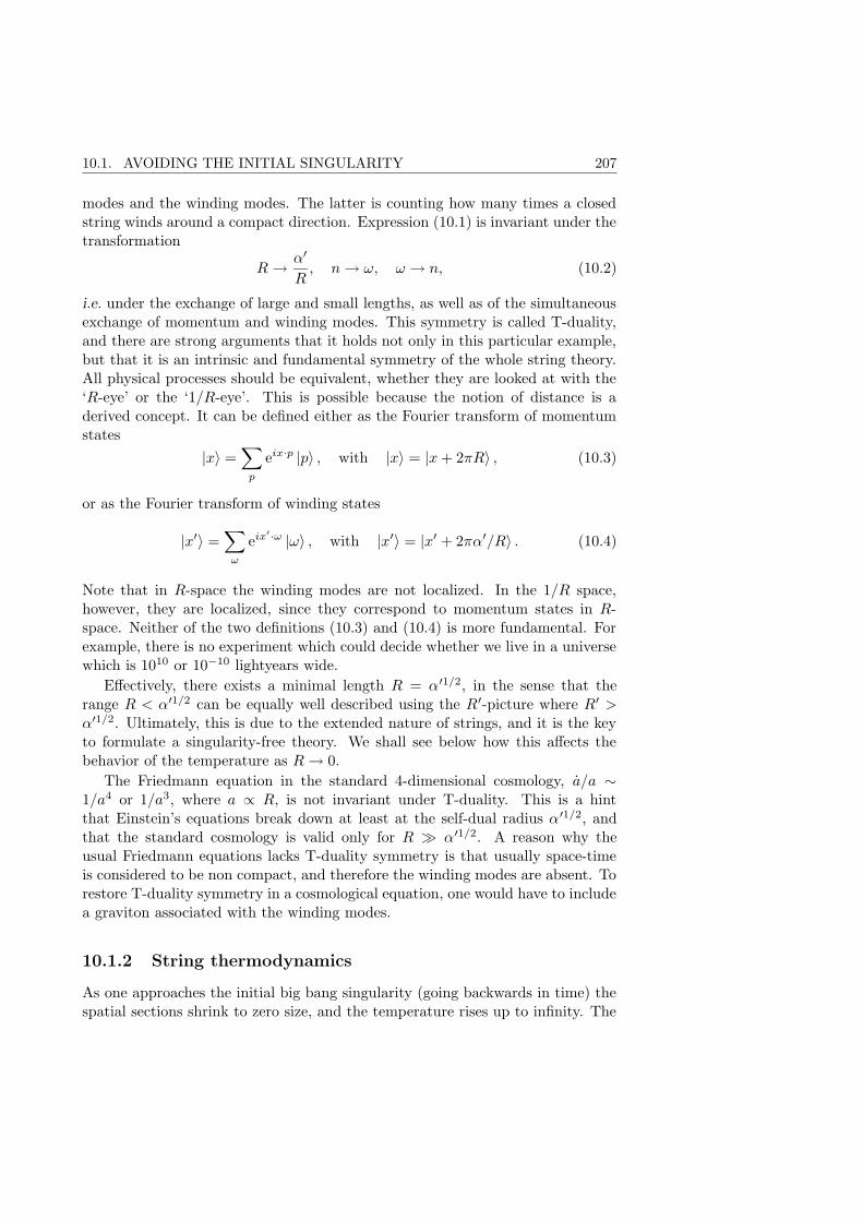
10.1. AVOIDING THE INITIAL SINGULARITY 207
modes and the winding modes. The latter is counting how many times a closedstring winds around a compact direction. Expression (10.1) is invariant under thetransformation
R→ α′
R, n→ ω, ω → n, (10.2)
i.e. under the exchange of large and small lengths, as well as of the simultaneousexchange of momentum and winding modes. This symmetry is called T-duality,and there are strong arguments that it holds not only in this particular example,but that it is an intrinsic and fundamental symmetry of the whole string theory.All physical processes should be equivalent, whether they are looked at with the‘R-eye’ or the ‘1/R-eye’. This is possible because the notion of distance is aderived concept. It can be defined either as the Fourier transform of momentumstates
|x〉 =∑
p
eix·p |p〉 , with |x〉 = |x+ 2πR〉 , (10.3)
or as the Fourier transform of winding states
|x′〉 =∑
ω
eix′·ω |ω〉 , with |x′〉 = |x′ + 2πα′/R〉 . (10.4)
Note that in R-space the winding modes are not localized. In the 1/R space,however, they are localized, since they correspond to momentum states in R-space. Neither of the two definitions (10.3) and (10.4) is more fundamental. Forexample, there is no experiment which could decide whether we live in a universewhich is 1010 or 10−10 lightyears wide.
Effectively, there exists a minimal length R = α′1/2, in the sense that therange R < α′1/2 can be equally well described using the R′-picture where R′ >α′1/2. Ultimately, this is due to the extended nature of strings, and it is the keyto formulate a singularity-free theory. We shall see below how this affects thebehavior of the temperature as R→ 0.
The Friedmann equation in the standard 4-dimensional cosmology, a/a ∼1/a4 or 1/a3, where a ∝ R, is not invariant under T-duality. This is a hintthat Einstein’s equations break down at least at the self-dual radius α′1/2, andthat the standard cosmology is valid only for R À α′1/2. A reason why theusual Friedmann equations lacks T-duality symmetry is that usually space-timeis considered to be non compact, and therefore the winding modes are absent. Torestore T-duality symmetry in a cosmological equation, one would have to includea graviton associated with the winding modes.
10.1.2 String thermodynamics
As one approaches the initial big bang singularity (going backwards in time) thespatial sections shrink to zero size, and the temperature rises up to infinity. The
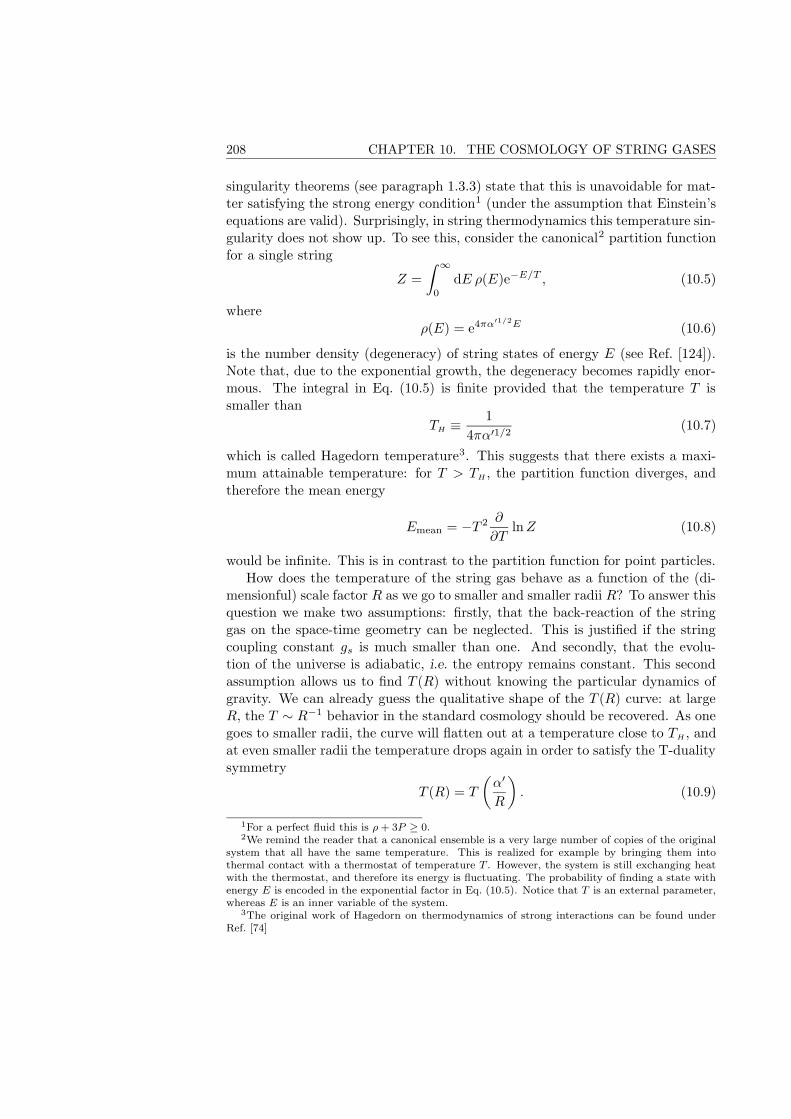
208 CHAPTER 10. THE COSMOLOGY OF STRING GASES
singularity theorems (see paragraph 1.3.3) state that this is unavoidable for mat-ter satisfying the strong energy condition1 (under the assumption that Einstein’sequations are valid). Surprisingly, in string thermodynamics this temperature sin-gularity does not show up. To see this, consider the canonical2 partition functionfor a single string
Z =
∫ ∞
0
dE ρ(E)e−E/T , (10.5)
where
ρ(E) = e4πα′1/2E (10.6)
is the number density (degeneracy) of string states of energy E (see Ref. [124]).Note that, due to the exponential growth, the degeneracy becomes rapidly enor-mous. The integral in Eq. (10.5) is finite provided that the temperature T issmaller than
TH ≡1
4πα′1/2(10.7)
which is called Hagedorn temperature3. This suggests that there exists a maxi-mum attainable temperature: for T > TH , the partition function diverges, andtherefore the mean energy
Emean = −T 2 ∂
∂TlnZ (10.8)
would be infinite. This is in contrast to the partition function for point particles.How does the temperature of the string gas behave as a function of the (di-
mensionful) scale factor R as we go to smaller and smaller radii R? To answer thisquestion we make two assumptions: firstly, that the back-reaction of the stringgas on the space-time geometry can be neglected. This is justified if the stringcoupling constant gs is much smaller than one. And secondly, that the evolu-tion of the universe is adiabatic, i.e. the entropy remains constant. This secondassumption allows us to find T (R) without knowing the particular dynamics ofgravity. We can already guess the qualitative shape of the T (R) curve: at largeR, the T ∼ R−1 behavior in the standard cosmology should be recovered. As onegoes to smaller radii, the curve will flatten out at a temperature close to TH , andat even smaller radii the temperature drops again in order to satisfy the T-dualitysymmetry
T (R) = T
(α′
R
). (10.9)
1For a perfect fluid this is ρ + 3P ≥ 0.2We remind the reader that a canonical ensemble is a very large number of copies of the original
system that all have the same temperature. This is realized for example by bringing them intothermal contact with a thermostat of temperature T . However, the system is still exchanging heatwith the thermostat, and therefore its energy is fluctuating. The probability of finding a state withenergy E is encoded in the exponential factor in Eq. (10.5). Notice that T is an external parameter,whereas E is an inner variable of the system.
3The original work of Hagedorn on thermodynamics of strong interactions can be found underRef. [74]
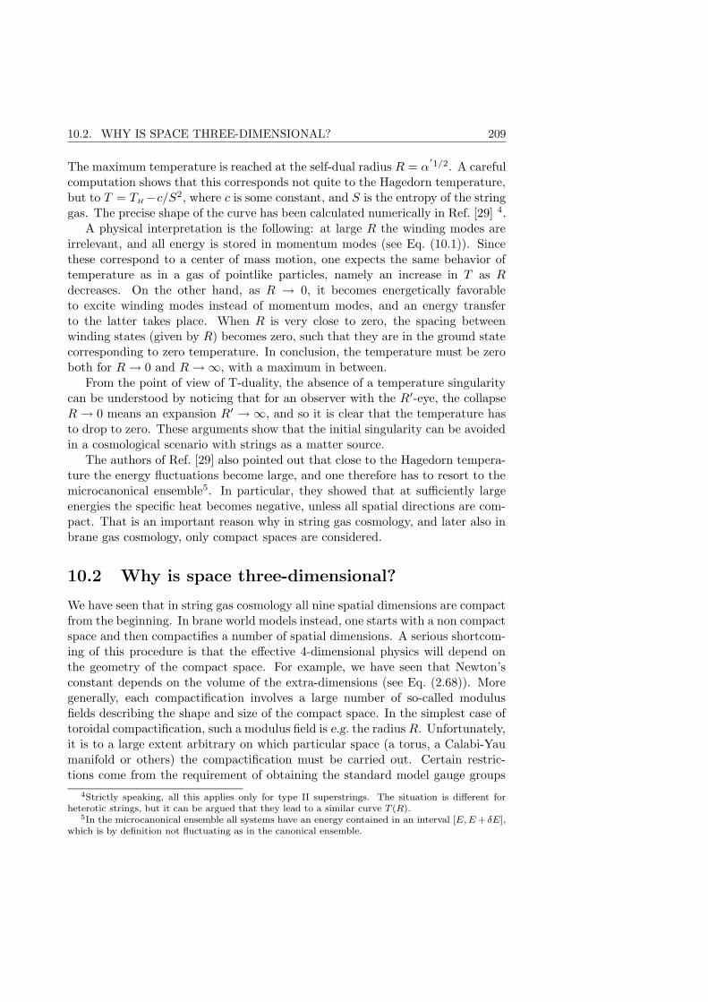
10.2. WHY IS SPACE THREE-DIMENSIONAL? 209
The maximum temperature is reached at the self-dual radius R = α′1/2. A careful
computation shows that this corresponds not quite to the Hagedorn temperature,but to T = TH−c/S2, where c is some constant, and S is the entropy of the stringgas. The precise shape of the curve has been calculated numerically in Ref. [29] 4.
A physical interpretation is the following: at large R the winding modes areirrelevant, and all energy is stored in momentum modes (see Eq. (10.1)). Sincethese correspond to a center of mass motion, one expects the same behavior oftemperature as in a gas of pointlike particles, namely an increase in T as Rdecreases. On the other hand, as R → 0, it becomes energetically favorableto excite winding modes instead of momentum modes, and an energy transferto the latter takes place. When R is very close to zero, the spacing betweenwinding states (given by R) becomes zero, such that they are in the ground statecorresponding to zero temperature. In conclusion, the temperature must be zeroboth for R→ 0 and R→∞, with a maximum in between.
From the point of view of T-duality, the absence of a temperature singularitycan be understood by noticing that for an observer with the R′-eye, the collapseR→ 0 means an expansion R′ →∞, and so it is clear that the temperature hasto drop to zero. These arguments show that the initial singularity can be avoidedin a cosmological scenario with strings as a matter source.
The authors of Ref. [29] also pointed out that close to the Hagedorn tempera-ture the energy fluctuations become large, and one therefore has to resort to themicrocanonical ensemble5. In particular, they showed that at sufficiently largeenergies the specific heat becomes negative, unless all spatial directions are com-pact. That is an important reason why in string gas cosmology, and later also inbrane gas cosmology, only compact spaces are considered.
10.2 Why is space three-dimensional?
We have seen that in string gas cosmology all nine spatial dimensions are compactfrom the beginning. In brane world models instead, one starts with a non compactspace and then compactifies a number of spatial dimensions. A serious shortcom-ing of this procedure is that the effective 4-dimensional physics will depend onthe geometry of the compact space. For example, we have seen that Newton’sconstant depends on the volume of the extra-dimensions (see Eq. (2.68)). Moregenerally, each compactification involves a large number of so-called modulusfields describing the shape and size of the compact space. In the simplest case oftoroidal compactification, such a modulus field is e.g. the radius R. Unfortunately,it is to a large extent arbitrary on which particular space (a torus, a Calabi-Yaumanifold or others) the compactification must be carried out. Certain restric-tions come from the requirement of obtaining the standard model gauge groups
4Strictly speaking, all this applies only for type II superstrings. The situation is different forheterotic strings, but it can be argued that they lead to a similar curve T (R).
5In the microcanonical ensemble all systems have an energy contained in an interval [E, E + δE],which is by definition not fluctuating as in the canonical ensemble.
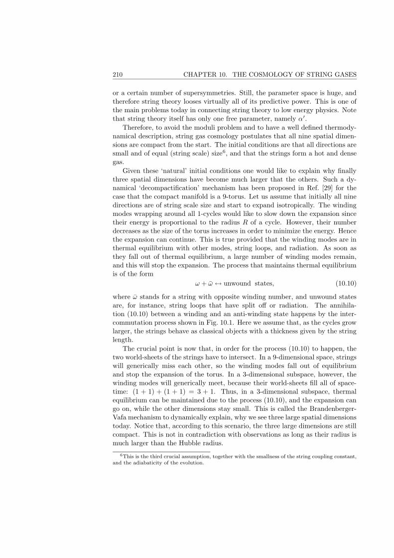
210 CHAPTER 10. THE COSMOLOGY OF STRING GASES
or a certain number of supersymmetries. Still, the parameter space is huge, andtherefore string theory looses virtually all of its predictive power. This is one ofthe main problems today in connecting string theory to low energy physics. Notethat string theory itself has only one free parameter, namely α′.
Therefore, to avoid the moduli problem and to have a well defined thermody-namical description, string gas cosmology postulates that all nine spatial dimen-sions are compact from the start. The initial conditions are that all directions aresmall and of equal (string scale) size6, and that the strings form a hot and densegas.
Given these ‘natural’ initial conditions one would like to explain why finallythree spatial dimensions have become much larger that the others. Such a dy-namical ‘decompactification’ mechanism has been proposed in Ref. [29] for thecase that the compact manifold is a 9-torus. Let us assume that initially all ninedirections are of string scale size and start to expand isotropically. The windingmodes wrapping around all 1-cycles would like to slow down the expansion sincetheir energy is proportional to the radius R of a cycle. However, their numberdecreases as the size of the torus increases in order to minimize the energy. Hencethe expansion can continue. This is true provided that the winding modes are inthermal equilibrium with other modes, string loops, and radiation. As soon asthey fall out of thermal equilibrium, a large number of winding modes remain,and this will stop the expansion. The process that maintains thermal equilibriumis of the form
ω + ω ↔ unwound states, (10.10)
where ω stands for a string with opposite winding number, and unwound statesare, for instance, string loops that have split off or radiation. The annihila-tion (10.10) between a winding and an anti-winding state happens by the inter-commutation process shown in Fig. 10.1. Here we assume that, as the cycles growlarger, the strings behave as classical objects with a thickness given by the stringlength.
The crucial point is now that, in order for the process (10.10) to happen, thetwo world-sheets of the strings have to intersect. In a 9-dimensional space, stringswill generically miss each other, so the winding modes fall out of equilibriumand stop the expansion of the torus. In a 3-dimensional subspace, however, thewinding modes will generically meet, because their world-sheets fill all of space-time: (1 + 1) + (1 + 1) = 3 + 1. Thus, in a 3-dimensional subspace, thermalequilibrium can be maintained due to the process (10.10), and the expansion cango on, while the other dimensions stay small. This is called the Brandenberger-Vafa mechanism to dynamically explain, why we see three large spatial dimensionstoday. Notice that, according to this scenario, the three large dimensions are stillcompact. This is not in contradiction with observations as long as their radius ismuch larger than the Hubble radius.
6This is the third crucial assumption, together with the smallness of the string coupling constant,and the adiabaticity of the evolution.
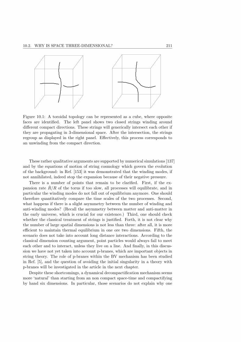
10.2. WHY IS SPACE THREE-DIMENSIONAL? 211
Figure 10.1: A toroidal topology can be represented as a cube, where oppositefaces are identified. The left panel shows two closed strings winding arounddifferent compact directions. These strings will generically intersect each other ifthey are propagating in 3-dimensional space. After the intersection, the stringsregroup as displayed in the right panel. Effectively, this process corresponds toan unwinding from the compact direction.
These rather qualitative arguments are supported by numerical simulations [137]and by the equations of motion of string cosmology which govern the evolutionof the background: in Ref. [153] it was demonstrated that the winding modes, ifnot annihilated, indeed stop the expansion because of their negative pressure.
There is a number of points that remain to be clarified. First, if the ex-pansion rate R/R of the torus if too slow, all processes will equilibrate, and inparticular the winding modes do not fall out of equilibrium anymore. One shouldtherefore quantitatively compare the time scales of the two processes. Second,what happens if there is a slight asymmetry between the number of winding andanti-winding modes? (Recall the asymmetry between matter and anti-matter inthe early universe, which is crucial for our existence.) Third, one should checkwhether the classical treatment of strings is justified. Forth, it is not clear whythe number of large spatial dimensions is not less than three: after all, it is moreefficient to maintain thermal equilibrium in one ore two dimensions. Fifth, thescenario does not take into account long distance interactions. According to theclassical dimension counting argument, point particles would always fail to meeteach other and to interact, unless they live on a line. And finally, in this discus-sion we have not yet taken into account p-branes, which are important objects instring theory. The role of p-branes within the BV mechanism has been studiedin Ref. [5], and the question of avoiding the initial singularity in a theory withp-branes will be investigated in the article in the next chapter.
Despite these shortcomings, a dynamical decompactification mechanism seemsmore ‘natural’ than starting from an non compact space-time and compactifyingby hand six dimensions. In particular, those scenarios do not explain why one
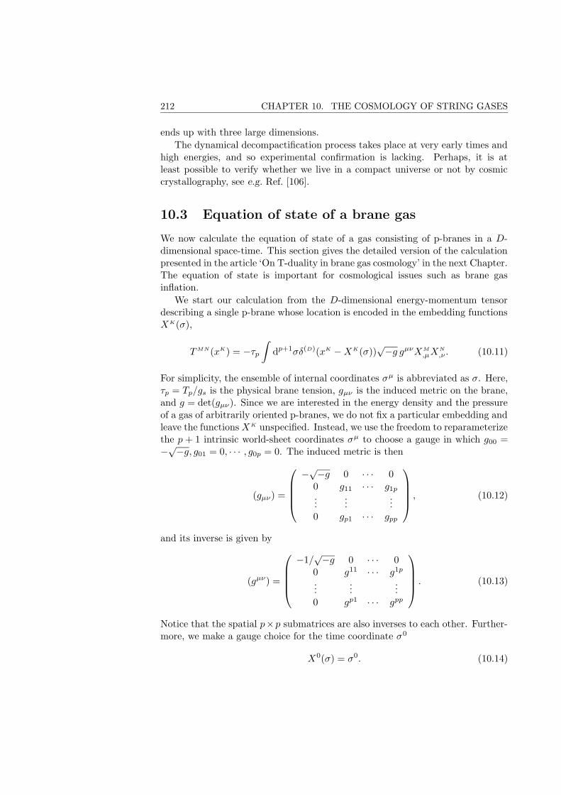
212 CHAPTER 10. THE COSMOLOGY OF STRING GASES
ends up with three large dimensions.
The dynamical decompactification process takes place at very early times andhigh energies, and so experimental confirmation is lacking. Perhaps, it is atleast possible to verify whether we live in a compact universe or not by cosmiccrystallography, see e.g. Ref. [106].
10.3 Equation of state of a brane gas
We now calculate the equation of state of a gas consisting of p-branes in a D-dimensional space-time. This section gives the detailed version of the calculationpresented in the article ‘On T-duality in brane gas cosmology’ in the next Chapter.The equation of state is important for cosmological issues such as brane gasinflation.
We start our calculation from the D-dimensional energy-momentum tensordescribing a single p-brane whose location is encoded in the embedding functionsXK(σ),
TMN(xK) = −τp∫
dp+1σδ(D)(xK −XK(σ))√−g gµνXM
,µXN
,ν . (10.11)
For simplicity, the ensemble of internal coordinates σµ is abbreviated as σ. Here,τp = Tp/gs is the physical brane tension, gµν is the induced metric on the brane,and g = det(gµν). Since we are interested in the energy density and the pressureof a gas of arbitrarily oriented p-branes, we do not fix a particular embedding andleave the functionsXK unspecified. Instead, we use the freedom to reparameterizethe p + 1 intrinsic world-sheet coordinates σµ to choose a gauge in which g00 =−√−g, g01 = 0, · · · , g0p = 0. The induced metric is then
(gµν) =
−√−g 0 · · · 00 g11 · · · g1p
......
...0 gp1 · · · gpp
, (10.12)
and its inverse is given by
(gµν) =
−1/√−g 0 · · · 00 g11 · · · g1p
......
...0 gp1 · · · gpp
. (10.13)
Notice that the spatial p×p submatrices are also inverses to each other. Further-more, we make a gauge choice for the time coordinate σ0
X0(σ) = σ0. (10.14)
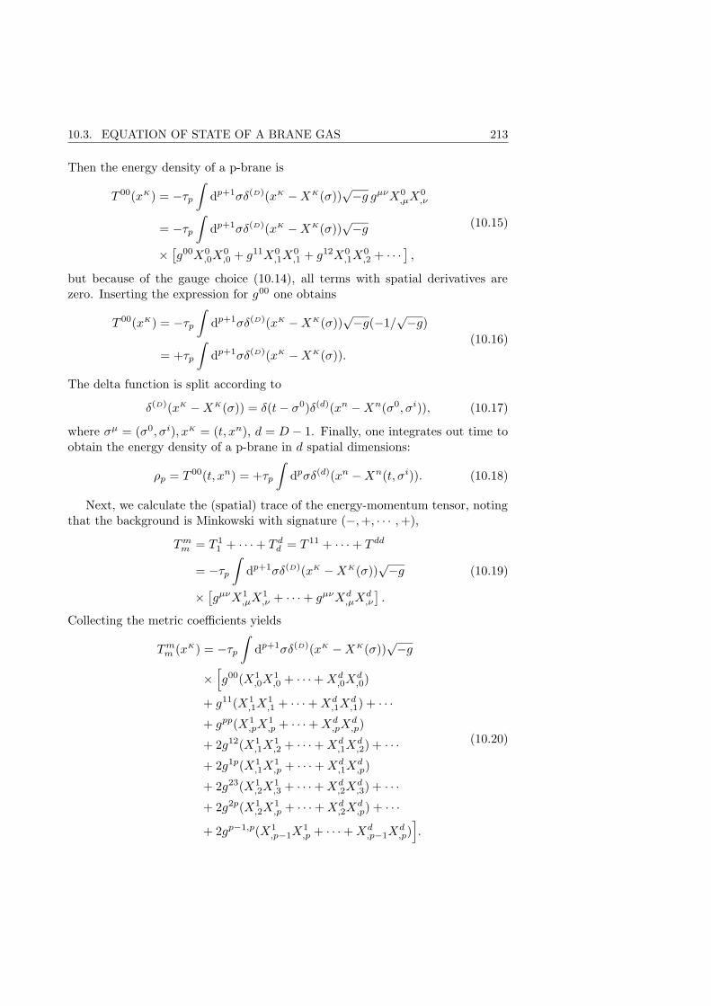
10.3. EQUATION OF STATE OF A BRANE GAS 213
Then the energy density of a p-brane is
T 00(xK) = −τp∫
dp+1σδ(D)(xK −XK(σ))√−g gµνX0
,µX0,ν
= −τp∫
dp+1σδ(D)(xK −XK(σ))√−g
×[g00X0
,0X0,0 + g11X0
,1X0,1 + g12X0
,1X0,2 + · · ·
],
(10.15)
but because of the gauge choice (10.14), all terms with spatial derivatives arezero. Inserting the expression for g00 one obtains
T 00(xK) = −τp∫
dp+1σδ(D)(xK −XK(σ))√−g(−1/
√−g)
= +τp
∫dp+1σδ(D)(xK −XK(σ)).
(10.16)
The delta function is split according to
δ(D)(xK −XK(σ)) = δ(t− σ0)δ(d)(xn −Xn(σ0, σi)), (10.17)
where σµ = (σ0, σi), xK = (t, xn), d = D − 1. Finally, one integrates out time toobtain the energy density of a p-brane in d spatial dimensions:
ρp = T 00(t, xn) = +τp
∫dpσδ(d)(xn −Xn(t, σi)). (10.18)
Next, we calculate the (spatial) trace of the energy-momentum tensor, notingthat the background is Minkowski with signature (−,+, · · · ,+),
Tmm = T 1
1 + · · ·+ T dd = T 11 + · · ·+ T dd
= −τp∫
dp+1σδ(D)(xK −XK(σ))√−g
×[gµνX1
,µX1,ν + · · ·+ gµνXd
,µXd,ν
].
(10.19)
Collecting the metric coefficients yields
Tmm (xK) = −τp
∫dp+1σδ(D)(xK −XK(σ))
√−g
×[g00(X1
,0X1,0 + · · ·+Xd
,0Xd,0)
+ g11(X1,1X
1,1 + · · ·+Xd
,1Xd,1) + · · ·
+ gpp(X1,pX
1,p + · · ·+Xd
,pXd,p)
+ 2g12(X1,1X
1,2 + · · ·+Xd
,1Xd,2) + · · ·
+ 2g1p(X1,1X
1,p + · · ·+Xd
,1Xd,p)
+ 2g23(X1,2X
1,3 + · · ·+Xd
,2Xd,3) + · · ·
+ 2g2p(X1,2X
1,p + · · ·+Xd
,2Xd,p) + · · ·
+ 2gp−1,p(X1,p−1X
1,p + · · ·+Xd
,p−1Xd,p)].
(10.20)
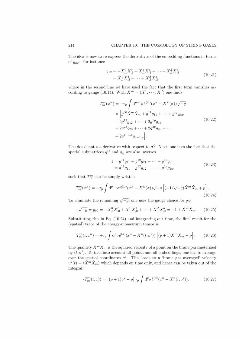
214 CHAPTER 10. THE COSMOLOGY OF STRING GASES
The idea is now to re-express the derivatives of the embedding functions in termsof gµν . For instance
g12 = −X0,1X
0,2 +X1
,1X1,2 + · · ·+Xd
,1Xd,2
= X1,1X
1,2 + · · ·+Xd
,1Xd,2,
(10.21)
where in the second line we have used the fact that the first term vanishes ac-cording to gauge (10.14). With Xm = (X1, · · · , Xd) one finds
Tmm (xK) = −τp
∫dp+1σδ(D)(xK −XK(σ))
√−g
×[g00XmXm + g11g11 + · · ·+ gppgpp
+ 2g12g12 + · · ·+ 2g1pg1p
+ 2g23g23 + · · ·+ 2g2pg2p + · · ·+ 2gp−1,pgp−1,p
].
(10.22)
The dot denotes a derivative with respect to σ0. Next, one uses the fact that thespatial submatrices gij and gij are also inverses
1 = g11g11 + g12g21 + · · ·+ g1pgp1
= g11g11 + g12g12 + · · ·+ g1pg1p,(10.23)
such that Tmm can be simply written
Tmm (xK) = −τp
∫dp+1σδ(D)(xK −XK(σ))
√−g[(−1/
√−g)XmXm + p].
(10.24)To eliminate the remaining
√−g, one uses the gauge choice for g00:
−√−g = g00 = −X0,0X
0,0 +X1
,0X1,0 + · · ·+Xd
,0Xd,0 = −1 + XmXm. (10.25)
Substituting this in Eq. (10.24) and integrating out time, the final result for the(spatial) trace of the energy-momentum tensor is
Tmm (t, xn) = +τp
∫dpσδ(d)(xn −Xn(t, σi))
[(p+ 1)XmXm − p
]. (10.26)
The quantity XmXm is the squared velocity of a point on the brane parameterizedby (t, σi). To take into account all points and all embeddings, one has to averageover the spatial coordinates σi. This leads to a ‘brane gas averaged’ velocityv2(t) = 〈XmXm〉 which depends on time only, and hence can be taken out of theintegral:
〈Tmm (t, ~x)〉 =
[(p+ 1)v2 − p
]τp
∫dpσδ(d)(xn −Xn(t, σi)). (10.27)
10.3. EQUATION OF STATE OF A BRANE GAS 215
Comparing Eq. (10.27) with the expression for the energy density (10.18), onefinds the equation of state
Pp =1
d〈Tm
m 〉 =[p+ 1
dv2 − p
d
]ρp, (10.28)
where Pp is the pressure of the p-brane gas. This pressure is within the range
−pdρp ≤ Pp ≤
1
dρp, (10.29)
where the lower bound is assumed in the non relativistic limit, v → 0, and theupper bound in the relativistic limit, v → 1.
To illustrate this formula, take for example a domain wall in three spatialdimensions (p = 2, d = 3). Then the equation of state (10.28) gives
P2 =
[v2 − 2
3
]ρ2, (10.30)
which in the limit v → 0 gives P2 = −23ρ2 as expected, and for v → 1 gives
P2 = 13ρ2.
It is amusing to note that the case p = d in the non relativistic limit leads toan equation of state P = −ρ. Hence a cosmological constant can be interpretedas a space-filling brane.

Chapter 11
On T-duality in brane gascosmology (article)

218 CHAPTER 11. ON T-DUALITY IN BRANE GAS COSMOLOGY
This chapter consists of the article ‘On T-duality in brane gas cosmology’,published in JCAP 06 (2003), see Ref. [20].
It is also available under http://lanl.arXiv.org/abs/hep-th/0208188.Like in the previous chapter, the pressure of a p-brane gas will be denoted by
Pp, because the letter P is here used for the p-brane momentum.
11.1. INTRODUCTION 219
On T-duality in brane gas cosmology
Timon BoehmDepartement de Physique Theorique, Universite de Geneve, 24 quai E. Ansermet, CH–1211 Geneva
4 Switzerland.
Robert BrandenbergerInstitut d’Astrophysique de Paris, 98bis Blvd. Arago, F-75014 Paris, France,
and
Physics Department, Brown University, Providence, RI 02912, USA.
In the context of homogeneous and isotropic superstring cosmology, the T-
duality symmetry of string theory has been used to argue that for a background
space-time described by dilaton gravity with strings as matter sources, the cos-
mological evolution of the universe will be non singular. In this letter we discuss
how T-duality extends to brane gas cosmology, an approximation in which the
background space-time is again described by dilaton gravity with a gas of branes
as a matter source. We conclude that the arguments for non singular cosmolo-
gical evolution remain valid.
PACS number: 98.80.Cq, 11.25.-w
11.1 Introduction
In [29] it was suggested that due to a new string theory-specific symmetry calledT-duality, string theory has the potential to resolve the initial singularity problemof standard big bang cosmology, a singularity which also plagues scalar field-driveninflationary cosmology [25, 24].
The framework of [29] was based on an approximation in which the mathema-tical background space-time is described by the equations of dilaton gravity (see[153, 157]), with the matter source consisting of a gas of strings. The backgroundspatial sections were assumed to be toroidal such as to admit one-cycles. Thus,the degrees of freedom of the string gas consist of winding modes in addition tothe momentum modes and the oscillatory modes. Then, both momentum andwinding numbers take on discrete values, and the energy spectrum of the theoryis invariant under inversion of the radii of the torus, i.e. R→ α′/R, where α′1/2 isthe string length ls. The mass of a state with momentum and winding numbersn and ω, respectively, in a compact space of radius R, is the same as that of astate with momentum and winding numbers ω and n, respectively, in the space ofradius α′/R. This symmetry was used to argue [29] that as the radii of the torusdecrease to very low values, no physical singularities will occur. Firstly, under
220 CHAPTER 11. ON T-DUALITY IN BRANE GAS COSMOLOGY
the assumption of thermal equilibrium, the temperature of a string gas at radiusR will be equal to the temperature of the string gas at radius α′/R. Secondly,any process computed for strings on a space with radius R, is identical to a dualprocess computed for strings on a space with radius α′/R. Therefore there ex-ists a ‘minimal’ radius α′1/2 in the sense that physics on length scales below thisradius can equally well be described by physics on length scales larger than that.
Since the work of [29] our knowledge of string theory has evolved in importantways. In particular, it has been realized [126] that string theory must containdegrees of freedom other than the perturbative string degrees of freedom usedin [29]. These new degrees of freedom are Dp-branes of various dimensionalities(depending on which string theory one is considering). Since the T-duality sym-metry was used in an essential way (see e.g. [125]) to arrive at the existence ofDp-branes (p-branes for short in the following), it is clear that T-duality symme-try will extend to a cosmological scenario including p-branes. However, since aT-duality transformation changes the dimensionality of branes, it is useful to ex-plicitly verify that the arguments of [29] for a non singular cosmological evolutioncarry over when the gas of perturbative string modes is generalized to a gas ofbranes. A model for superstring cosmology in which the background space-timeis described (as in [153, 157]) by dilaton gravity, and the matter source is a gasof branes, has recently been studied under the name of “brane gas cosmology”[5, 27] (see also [57, 58] for extensions to backgrounds which are not toroidal, and[161] for an extension to an anisotropic background).
In this letter, we establish the explicit action of T-duality in the context ofbrane gas cosmology on a toroidal background. For a solution of the backgroundgeometry appropriate for cosmological considerations in which the radii of thetorus are decreasing from large to small values as we go back in time, we mustconsider T-dualizing in all spatial dimensions. We demonstrate that the massspectrum of branes remains invariant under this action. Thus, if the backgrounddynamics are adiabatic, then the temperature of the brane gas will be invariantunder the change R→ α′/R, i.e.
T (R) = T
(α′
R
), (11.1)
thus demonstrating that superstring cosmology can avoid the temperature sin-gularity problem of standard and inflationary cosmology. In the appendix wemake further remarks on why we expect brane gas cosmology to be non singu-lar. Another crucial assumption is that the string coupling constant gs is small(compared to one) such that back-reactions of the string and brane gas on thecurvature of space-time can be ignored. Similarly, our results can be used to showthat the arguments for the existence of a minimal physical length given in [29]extend to brane gas cosmology.
The outline of this letter is as follows. In the following section we give abrief review of brane gas cosmology. In section 11.3 we derive the energy, themomentum, and the pressure for p-branes. Next, we review the action of T-duality
11.2. REVIEW OF BRANE GAS COSMOLOGY 221
on winding states of p-branes. The main section of this letter is section 11.5 inwhich we show that the mass spectrum of a p-brane gas of superstring theory isinvariant under T-duality. Section 11.6 contains a discussion of some implicationsof the result, and conclusions.
11.2 Review of brane gas cosmology
As already mentioned in the introduction, the framework of brane gas cosmologyconsists of a homogeneous and isotropic background of dilaton gravity coupled toa gas of p-branes as a matter source. We are living in the bulk1.
The initial conditions in the early universe are ‘conservative’ and ‘democratic’;conservative in the sense that they are close to the initial conditions assumed tohold in standard big bang cosmology (i.e. a hot dense gas of matter), democraticin the sense that all 9 spatial dimensions of critical string theory are consideredon an equal basis2. Thus, matter is taken to be a gas of p-branes of all allowedvalues of p in thermal equilibrium. In particular, all modes of the branes areexcited, including the winding modes.
The background space-time is taken to be R × T 9 where T 9 denotes a nine-torus. The key feature of T 9 which is used in the analysis is the fact that it admitsone-cycles which makes it possible for closed strings to have conserved windingnumbers3. It is also assumed that the initial radius in each toroidal direction isthe same, and comparable to the self-dual radius α′1/2. Initially, all directionsare expanding isotropically with R > α′1/2 (the extension to anisotropic initialconditions has recently been considered in [161]).
As shown in this letter, as a consequence of T-duality symmetry, brane gas cos-mology provides a background evolution without cosmological singularities. Thescenario also provides a possible dynamical explanation for why only three spatialdimensions can become large. Winding modes (and thus T-duality) play a cru-cial role in the argument. Let us first focus on the winding modes of fundamentalstrings [29].
The winding and anti-winding modes ω and ω of the strings are initially inthermal equilibrium with the other states in the string gas. Thermal equilibrium
1In this sense, brane gas cosmology is completely different in ideology than brane world scenariosin which it is assumed (in general without any dynamical explanation) that we live on a specificbrane embedded in a warped bulk space-time. From the point of view of heterotic M theory [77],our considerations should be viewed as applying to the 10-dimensional orbifold space-time on whichwe live.
2For consistency, critical superstring theories need a 10 dimensional target space-time which isin apparent contradiction with the observed four. Usually it is assumed that six dimensions arecompactified from the outset due to some unknown physics. However, following the usual approachin cosmology it seems more natural that initially all nine spatial dimensions were compact and small,and that three of them have grown large by a dynamical decompactification process. A correspondingscenario was originally proposed in [29].
3Recently, the scenario of [29, 5] was generalized [57, 58] to spatial backgrounds such as Calabi-Yaumanifolds which admit 2-cycles but no 1-cycles.
222 CHAPTER 11. ON T-DUALITY IN BRANE GAS COSMOLOGY
is maintained by the process
ω + ω À loops, radiation. (11.2)
When strings cross each other, they can intercommute such that a winding andan anti-winding mode annihilate, producing fundamental string loops or radia-tion without winding number. This process is analogous to infinite cosmic stringsintersecting and producing cosmic string loops and radiation during their inter-action (see e.g. [158, 28] for reviews of cosmic string dynamics).
As the spatial sections continue to expand, matter degrees of freedom willgradually fall out of equilibrium. In the context of string gas cosmology withR > α′1/2, the winding strings are the heaviest objects and will hence fall out ofequilibrium first. Since the energy of a winding mode is proportional to R, New-tonian intuition would imply that the presence of winding modes would preventfurther expansion. This is contrary to what would be obtained by using the Ein-stein equations. However, the equations of dilaton gravity yield a similar result towhat is obtained from Newtonian intuition [153]: the presence of winding modes(with negative pressure) acts as a confining potential for the scale factor.
As long as winding modes are in thermal equilibrium, the total energy canbe minimized by transferring it to momentum or oscillatory modes (of the fun-damental string). Thereby, the number of winding modes decreases, and theexpansion can go on. However, if the winding modes fall out of equilibrium, suchthat there is a large number of them left, the expansion is slowed down and even-tually stopped. If we now try to make d of the original 9 spatial dimensions muchlarger than the string scale, then an obstruction is encountered if d > 3: in thiscase the probability for crossing and therefore for equilibrating according to theprocess (11.2) is zero. On the other hand, in a three-dimensional subspace of thenine-torus, two strings will generically meet. Therefore, the winding modes canannihilate, thermal equilibrium can be maintained, and, since the decay modes ofthe winding strings have positive pressure, the expansion can go on4. As a result,there is no topological obstruction to three dimensions of the torus growing largewhile the other six are staying small of size R ∼ α′1/2. Large compact dimensionsare not in contradiction with observations if their radius is bigger than the Hubbleradius today.
It is not hard to include p-branes into the above scenario [5]. Now the initialstate is a hot, dense gas of all branes allowed in a particular theory. In particular,brane winding modes are excited, in addition to modes corresponding to fluctua-tions of the brane. Since the winding modes play the most important role in thedynamical decompactification mechanism of [29, 5], we will focus our attentionon these modes. The analogous classical counting argument as given above forstrings yields the result that p-brane winding modes can interact in at most 2p+1
4Since quantum mechanically, the thickness of the strings is given by the string length [89], itis important for the brane gas scenario that the initial size of the spatial sections was string scale.Otherwise, it would always be the total dimensionality of space which would be relevant in theclassical counting argument of [29], and there could be no expansion in any direction.
11.3. ENERGY, MOMENTUM, AND PRESSURE OF P-BRANES 223
spatial dimensions. Since for weak string coupling and for spatial sizes larger thanthe self-dual radius the mass of a p-brane (with a fixed winding number in all ofits p spatial dimensions) increases as p increases, p-branes will fall out of equilib-rium earlier the larger p is. Thus, for instance in a scenario with 2-branes, thesewill fall out of equilibrium before the fundamental strings and allow five spatialdimensions to start to grow [5]. Within these five spatial dimensions, the funda-mental string winding modes will then allow only a three-dimensional subspace tobecome macroscopic. Thus there is no topological obstruction to the dynamicalgeneration of a hierarchy of internal dimensions.
11.3 Energy, momentum, and pressure of p-branes
This section is devoted to the derivation of physical quantities describing the branegas which determine the cosmological evolution of the background space-time.
Starting from the Nambu–Goto action, we obtain expressions for the energyand the momentum of a p-brane in D = d+ 1 dimensional space-time. We showthat there is no momentum flowing along the p tangential directions. From theenergy–momentum tensor one can also define a pressure, and hence an equationof state, for the whole brane gas. Even though some of the results in this sectionare already known, we find it useful to give a self-consistent overview.
Let σ = (σ0, σi), i = 1, · · · , p, denote intrinsic coordinates on the world-sheet of a p-brane. Its position (or embedding) in D-dimensional space timeis described by xM = XM(σ), where M = 0, · · · , d, and the induced metric isgµν = ηMNX
M,µX
N,ν , where µ, ν = 0, · · · , p.
In the string frame, the Nambu–Goto action is
Sp = −Tp
∫dp+1σe−Φ√−g , (11.3)
where Tp denotes the tension of a p-brane, g = det(gµν), and Φ is the dilaton ofthe compactified theory. For our adiabatic considerations, we assume that it isconstant (taking its asymptotic value), and absorb it into a physical tension
τp = e−ΦTp =Tp
gs=
1
(2π)p
1
gsα′(p+1)/2, (11.4)
where in the final step we have used the explicit expression for Tp (see e.g. [125]).Note that for any p-brane τp goes like 1/gs, and that hence, in the weak stringcoupling regime which we are considering, the branes are heavy. The action (11.3)can be written as an integral over D-dimensional space-time
Sp =
∫dDx
(−τp
∫dp+1σδ(D)(xK −XK(σ))
√−g). (11.5)
As the integration domain is a torus, both integrals are finite.
224 CHAPTER 11. ON T-DUALITY IN BRANE GAS COSMOLOGY
Varying the action (11.5) with respect to the background metric and comparingwith the usual definition of the space-time energy-momentum tensor, one obtains5
TMN(xK) = −τp∫
dp+1σδ(D)(xK −XK(σ))√−g gµνXM
,µXN
,ν . (11.6)
The Nambu–Goto action (11.3) is invariant under p + 1 reparametrizationsσ → σ(σ), and we can use this freedom to choose
g00 = −√−g , g0i = 0 . (11.7)
Notice that for the spatial sub-matrix with indices i, j, k = 1, · · · , p, det(gij) =−√−g and gikgkj = δi
j . By choosing the gauge (11.7), we do not specify aparticular embedding. This will be convenient later when treating a brane gas,where the branes have arbitrary orientations. Furthermore, it is consistent to setX0 = σ0.
To calculate the energy Ep of a p-brane, one observes that in the gauge (11.7)
gµνX0,µX
0,ν = g00 = − 1√−g
⇒ T 00(xK) = τp
∫dp+1σδ(D)(xK −XK(σ)) . (11.8)
Writing xK = (t, xn), n = 1, · · · , d, and splitting the delta-function into a product,the integral over σ0 can be carried out. The energy density of a p-brane in d spatialdimensions is then
ρp ≡ T 00(t, xn) = τp
∫dpσδ(d)(xn −Xn(t, σi)), (11.9)
and its total energy is
Ep =
∫ddx ρp = τp
∫dpσ = τpVolp . (11.10)
The volume of a p-brane in its rest frame, Volp, is finite as the brane is wrappedaround a torus. Eq. (11.10) provides a formula for the lowest mass state, Mp = Ep,which will be used in section 11.5. As expected intuitively, the minimal mass isequal to the tension times the volume of a brane.
To calculate the space-time momentum P np of a p-brane, one first evaluates
gµνX0,µX
n,ν = − Xn
,0√−g
⇒ T 0n(xK) = τp
∫dp+1σδ(D)(xK −XK(σ))Xn
,0 . (11.11)
5In curved backgrounds, with metric GMN say, the energy-momentum tensor gets multiplied with√−det(GMN ).
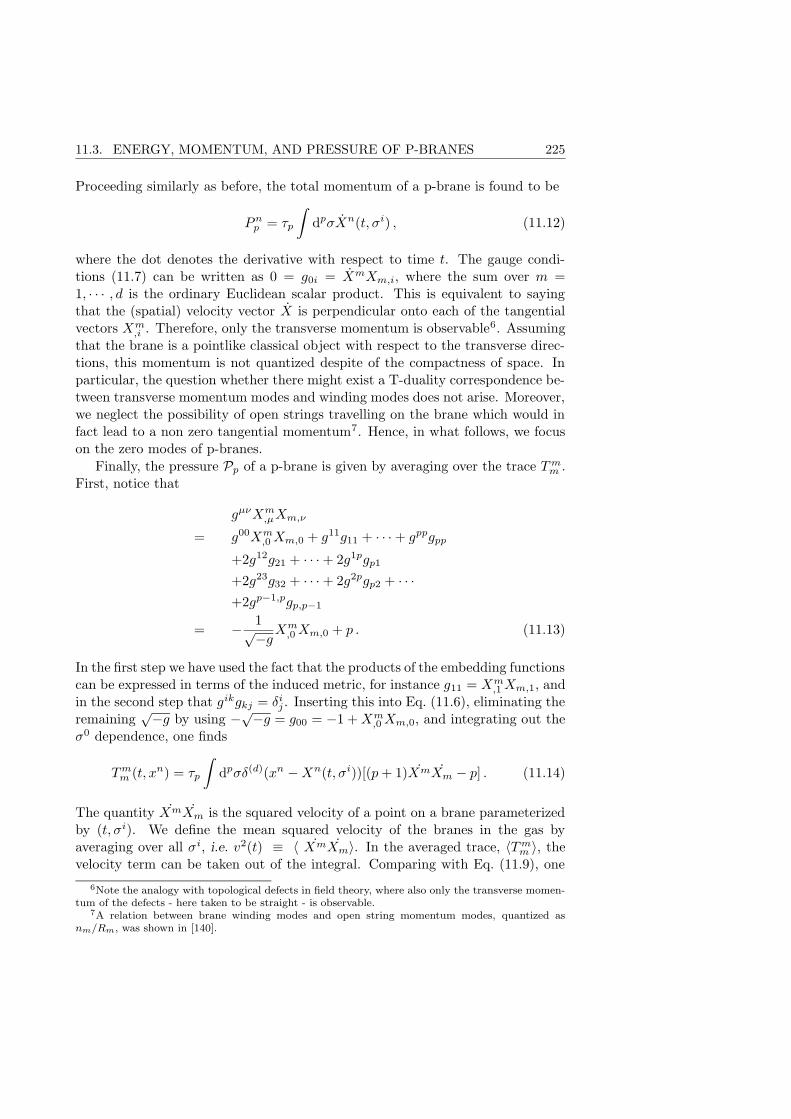
11.3. ENERGY, MOMENTUM, AND PRESSURE OF P-BRANES 225
Proceeding similarly as before, the total momentum of a p-brane is found to be
Pnp = τp
∫dpσXn(t, σi) , (11.12)
where the dot denotes the derivative with respect to time t. The gauge condi-tions (11.7) can be written as 0 = g0i = XmXm,i, where the sum over m =1, · · · , d is the ordinary Euclidean scalar product. This is equivalent to sayingthat the (spatial) velocity vector X is perpendicular onto each of the tangentialvectors Xm
,i . Therefore, only the transverse momentum is observable6. Assumingthat the brane is a pointlike classical object with respect to the transverse direc-tions, this momentum is not quantized despite of the compactness of space. Inparticular, the question whether there might exist a T-duality correspondence be-tween transverse momentum modes and winding modes does not arise. Moreover,we neglect the possibility of open strings travelling on the brane which would infact lead to a non zero tangential momentum7. Hence, in what follows, we focuson the zero modes of p-branes.
Finally, the pressure Pp of a p-brane is given by averaging over the trace Tmm .
First, notice that
gµνXm,µXm,ν
= g00Xm,0Xm,0 + g11g11 + · · ·+ gppgpp
+2g12g21 + · · ·+ 2g1pgp1
+2g23g32 + · · ·+ 2g2pgp2 + · · ·+2gp−1,pgp,p−1
= − 1√−gXm,0Xm,0 + p . (11.13)
In the first step we have used the fact that the products of the embedding functionscan be expressed in terms of the induced metric, for instance g11 = Xm
,1Xm,1, andin the second step that gikgkj = δi
j . Inserting this into Eq. (11.6), eliminating theremaining
√−g by using −√−g = g00 = −1 +Xm,0Xm,0, and integrating out the
σ0 dependence, one finds
Tmm (t, xn) = τp
∫dpσδ(d)(xn −Xn(t, σi))[(p+ 1)XmXm − p] . (11.14)
The quantity XmXm is the squared velocity of a point on a brane parameterizedby (t, σi). We define the mean squared velocity of the branes in the gas byaveraging over all σi, i.e. v2(t) ≡ 〈 XmXm〉. In the averaged trace, 〈Tm
m 〉, thevelocity term can be taken out of the integral. Comparing with Eq. (11.9), one
6Note the analogy with topological defects in field theory, where also only the transverse momen-tum of the defects - here taken to be straight - is observable.
7A relation between brane winding modes and open string momentum modes, quantized asnm/Rm, was shown in [140].
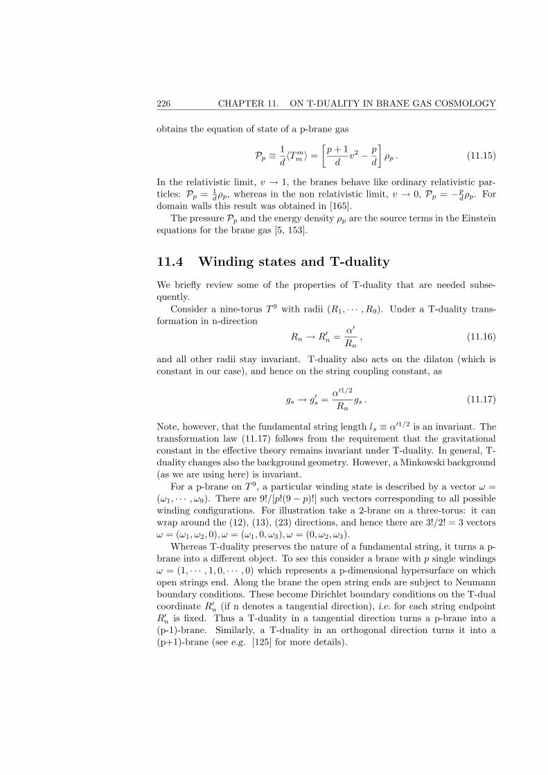
226 CHAPTER 11. ON T-DUALITY IN BRANE GAS COSMOLOGY
obtains the equation of state of a p-brane gas
Pp ≡1
d〈Tm
m 〉 =[p+ 1
dv2 − p
d
]ρp . (11.15)
In the relativistic limit, v → 1, the branes behave like ordinary relativistic par-ticles: Pp = 1
dρp, whereas in the non relativistic limit, v → 0, Pp = −pdρp. For
domain walls this result was obtained in [165].
The pressure Pp and the energy density ρp are the source terms in the Einsteinequations for the brane gas [5, 153].
11.4 Winding states and T-duality
We briefly review some of the properties of T-duality that are needed subse-quently.
Consider a nine-torus T 9 with radii (R1, · · · , R9). Under a T-duality trans-formation in n-direction
Rn → R′n =
α′
Rn, (11.16)
and all other radii stay invariant. T-duality also acts on the dilaton (which isconstant in our case), and hence on the string coupling constant, as
gs → g′s =α′1/2
Rngs . (11.17)
Note, however, that the fundamental string length ls ≡ α′1/2 is an invariant. Thetransformation law (11.17) follows from the requirement that the gravitationalconstant in the effective theory remains invariant under T-duality. In general, T-duality changes also the background geometry. However, a Minkowski background(as we are using here) is invariant.
For a p-brane on T 9, a particular winding state is described by a vector ω =(ω1, · · · , ω9). There are 9!/[p!(9 − p)!] such vectors corresponding to all possiblewinding configurations. For illustration take a 2-brane on a three-torus: it canwrap around the (12), (13), (23) directions, and hence there are 3!/2! = 3 vectorsω = (ω1, ω2, 0), ω = (ω1, 0, ω3), ω = (0, ω2, ω3).
Whereas T-duality preserves the nature of a fundamental string, it turns a p-brane into a different object. To see this consider a brane with p single windingsω = (1, · · · , 1, 0, · · · , 0) which represents a p-dimensional hypersurface on whichopen strings end. Along the brane the open string ends are subject to Neumannboundary conditions. These become Dirichlet boundary conditions on the T-dualcoordinate R′
n (if n denotes a tangential direction), i.e. for each string endpointR′
n is fixed. Thus a T-duality in a tangential direction turns a p-brane into a(p-1)-brane. Similarly, a T-duality in an orthogonal direction turns it into a(p+1)-brane (see e.g. [125] for more details).
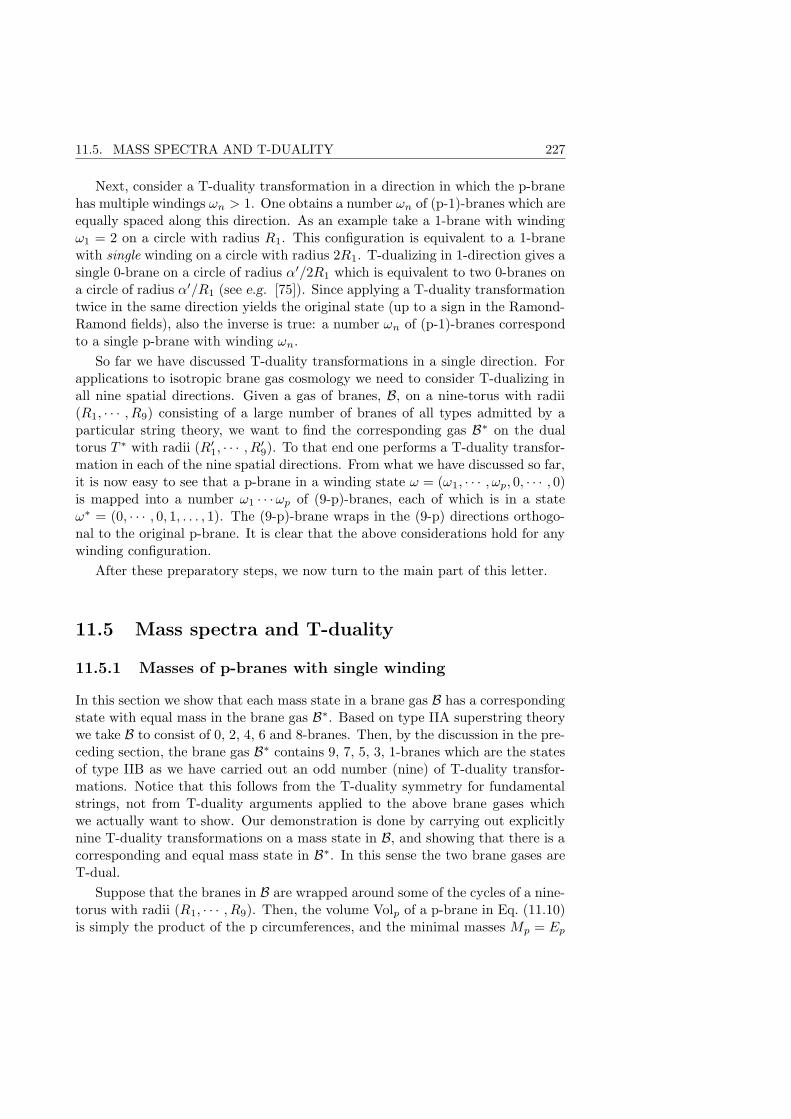
11.5. MASS SPECTRA AND T-DUALITY 227
Next, consider a T-duality transformation in a direction in which the p-branehas multiple windings ωn > 1. One obtains a number ωn of (p-1)-branes which areequally spaced along this direction. As an example take a 1-brane with windingω1 = 2 on a circle with radius R1. This configuration is equivalent to a 1-branewith single winding on a circle with radius 2R1. T-dualizing in 1-direction gives asingle 0-brane on a circle of radius α′/2R1 which is equivalent to two 0-branes ona circle of radius α′/R1 (see e.g. [75]). Since applying a T-duality transformationtwice in the same direction yields the original state (up to a sign in the Ramond-Ramond fields), also the inverse is true: a number ωn of (p-1)-branes correspondto a single p-brane with winding ωn.
So far we have discussed T-duality transformations in a single direction. Forapplications to isotropic brane gas cosmology we need to consider T-dualizing inall nine spatial directions. Given a gas of branes, B, on a nine-torus with radii(R1, · · · , R9) consisting of a large number of branes of all types admitted by aparticular string theory, we want to find the corresponding gas B∗ on the dualtorus T ∗ with radii (R′
1, · · · , R′9). To that end one performs a T-duality transfor-
mation in each of the nine spatial directions. From what we have discussed so far,it is now easy to see that a p-brane in a winding state ω = (ω1, · · · , ωp, 0, · · · , 0)is mapped into a number ω1 · · ·ωp of (9-p)-branes, each of which is in a stateω∗ = (0, · · · , 0, 1, . . . , 1). The (9-p)-brane wraps in the (9-p) directions orthogo-nal to the original p-brane. It is clear that the above considerations hold for anywinding configuration.
After these preparatory steps, we now turn to the main part of this letter.
11.5 Mass spectra and T-duality
11.5.1 Masses of p-branes with single winding
In this section we show that each mass state in a brane gas B has a correspondingstate with equal mass in the brane gas B∗. Based on type IIA superstring theorywe take B to consist of 0, 2, 4, 6 and 8-branes. Then, by the discussion in the pre-ceding section, the brane gas B∗ contains 9, 7, 5, 3, 1-branes which are the statesof type IIB as we have carried out an odd number (nine) of T-duality transfor-mations. Notice that this follows from the T-duality symmetry for fundamentalstrings, not from T-duality arguments applied to the above brane gases whichwe actually want to show. Our demonstration is done by carrying out explicitlynine T-duality transformations on a mass state in B, and showing that there is acorresponding and equal mass state in B∗. In this sense the two brane gases areT-dual.
Suppose that the branes in B are wrapped around some of the cycles of a nine-torus with radii (R1, · · · , R9). Then, the volume Volp of a p-brane in Eq. (11.10)is simply the product of the p circumferences, and the minimal masses Mp = Ep
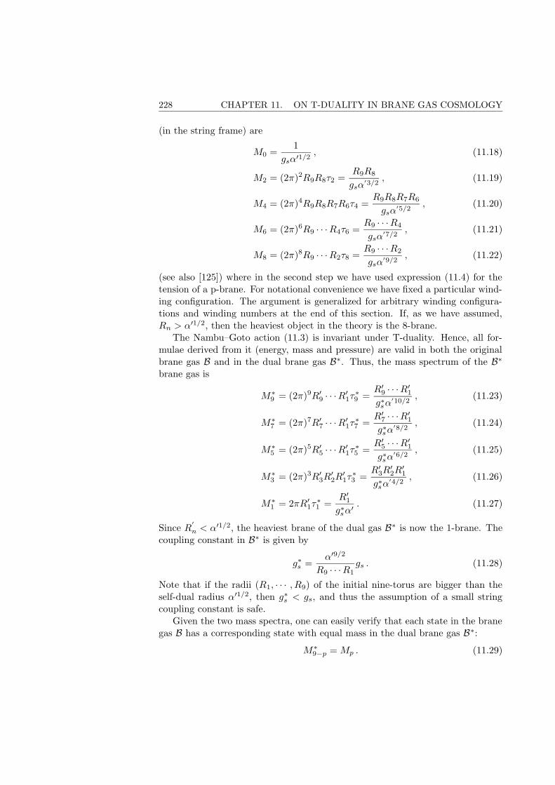
228 CHAPTER 11. ON T-DUALITY IN BRANE GAS COSMOLOGY
(in the string frame) are
M0 =1
gsα′1/2, (11.18)
M2 = (2π)2R9R8τ2 =R9R8
gsα′3/2
, (11.19)
M4 = (2π)4R9R8R7R6τ4 =R9R8R7R6
gsα′5/2
, (11.20)
M6 = (2π)6R9 · · ·R4τ6 =R9 · · ·R4
gsα′7/2
, (11.21)
M8 = (2π)8R9 · · ·R2τ8 =R9 · · ·R2
gsα′9/2
, (11.22)
(see also [125]) where in the second step we have used expression (11.4) for thetension of a p-brane. For notational convenience we have fixed a particular wind-ing configuration. The argument is generalized for arbitrary winding configura-tions and winding numbers at the end of this section. If, as we have assumed,Rn > α′1/2, then the heaviest object in the theory is the 8-brane.
The Nambu–Goto action (11.3) is invariant under T-duality. Hence, all for-mulae derived from it (energy, mass and pressure) are valid in both the originalbrane gas B and in the dual brane gas B∗. Thus, the mass spectrum of the B∗
brane gas is
M∗9 = (2π)9R′
9 · · ·R′1τ
∗9 =
R′9 · · ·R′
1
g∗sα′10/2
, (11.23)
M∗7 = (2π)7R′
7 · · ·R′1τ
∗7 =
R′7 · · ·R′
1
g∗sα′8/2
, (11.24)
M∗5 = (2π)5R′
5 · · ·R′1τ
∗5 =
R′5 · · ·R′
1
g∗sα′6/2
, (11.25)
M∗3 = (2π)3R′
3R′2R
′1τ
∗3 =
R′3R
′2R
′1
g∗sα′4/2
, (11.26)
M∗1 = 2πR′
1τ∗1 =
R′1
g∗sα′ . (11.27)
Since R′
n < α′1/2, the heaviest brane of the dual gas B∗ is now the 1-brane. Thecoupling constant in B∗ is given by
g∗s =α′9/2
R9 · · ·R1gs . (11.28)
Note that if the radii (R1, · · · , R9) of the initial nine-torus are bigger than theself-dual radius α′1/2, then g∗s < gs, and thus the assumption of a small stringcoupling constant is safe.
Given the two mass spectra, one can easily verify that each state in the branegas B has a corresponding state with equal mass in the dual brane gas B∗:
M∗9−p = Mp . (11.29)
11.5. MASS SPECTRA AND T-DUALITY 229
This establishes explicitly that the T-duality of the string gas used in [29] extendsto the brane gas cosmology of [5].
As an explicit example, consider a 2-brane wrapped around the 8 and 9 direc-tions. Its mass is (11.19)
M2 =R8R9
gsα′3/2
. (11.30)
If we replace the string coupling constant gs by the dual string coupling constantg∗s via (11.28), and the radii R8 and R9 by the dual radii R
′
8 and R′
9 via (11.16),one obtains
M2 =R
′
1 · · ·R′
7
g∗sα′8/2
= M∗7 . (11.31)
In the above example, we have specified a particular winding configuration forsimplicity, but clearly the argument holds as well in the general case, where ap-brane wraps around some directions n1 · · ·np:
Mp = (2π)pRn1 · · ·Rnpτp =Rn1 · · ·Rnp
gsα′(p+1)/2
. (11.32)
Via the same steps as in the above example, it follows that
M∗9−p = (2π)9−pR′
m1· · ·R′
m9−pτ∗9−p =
R′m1· · ·R′
m9−p
g∗sα′(10−p)/2
= Mp , (11.33)
where m1, · · · ,m9−p 6= n1, · · · , np.
11.5.2 Multiple windings
Consider now a p-brane with multiple windings ω = (ω1, · · · , ωp, 0, · · · , 0). Itsmass is
Mp(ω) = ω1 · · ·ωpMp . (11.34)
In the B∗ brane gas this corresponds to a number ω1 · · ·ωp of (9-p)-branes eachwith winding ω∗ = (0, · · · , 0, 1, · · · , 1) and mass M ∗
9−p. Since M∗9−p = Mp, the
total mass of this ‘multi-brane’ state is equal to the mass of the original brane,namely
(ω1 · · ·ωp)M∗9−p = Mp(ω) , (11.35)
which establishes the correspondence of B and B∗ in the case of multiple windings.One should also add fundamental strings to the brane gas B. Since their mass
squared is
M2 =
(nn
Rn
)2
+
(ωnRn
α′
)2
, (11.36)
is its clear that every fundamental string state in B has a corresponding state inB∗ when nn ↔ ωn.
230 CHAPTER 11. ON T-DUALITY IN BRANE GAS COSMOLOGY
11.6 Cosmological implications and discussion
We have demonstrated explicitly how T-duality acts on a brane gas in a toroidalcosmological background, and have in particular shown that the mass spectrum ofthe theory is invariant under T-duality. Thus, the arguments of [29] which led tothe conclusion that cosmological singularities can be avoided in string cosmologyextend to brane gas cosmology.
Whereas T-duality does not change the nature of fundamental strings, butsimply interchanges winding and momentum numbers, it changes the nature ofbranes: after T-dualizing in all d spatial dimensions, a p-brane becomes a (d-p)-brane which, however, was shown to have the same mass as the ‘original’ brane.
In [5] it was shown that the dynamical decompactification mechanism pro-posed in [29] remains valid if, in addition to fundamental strings, the degreesof freedom of type IIA superstring theory are enclosed. We briefly comment onthe decompactification mechanism in the presence of a type IIB brane gas on anine-torus. As before, we assume a hot, dense initial state where, in particular,the brane winding modes are excited and in thermal equilibrium with the otherdegrees of freedom. All directions of the torus are roughly of string scale size, ls,and start to expand isotropically. For the 9,7, and 5-brane winding modes thereis no dimensional obstruction to continuously meet and to remain in equilibrium,thereby transferring their energy to less costly momentum or oscillatory modes:these degrees of freedom do not constrain the number of expanding dimensions.However, the 3-branes allow only seven dimensions to grow further, and out ofthese, three dimensions can become large when 1-brane and string winding modeshave disappeared. As far as the ‘intercommutation’ and equilibration process isconcerned, the 1-branes and the strings play the same role, but since the windingmodes of the former are heavier ( R
gsα′À R
α′at weak coupling), they disappear
earlier.
We have focused our attention on how T-duality acts on brane winding modes.However, since in a hot and dense initial state we expect all degrees of freedom ofa brane to be excited, we should also include transverse fluctuations (oscillatorymodes) in our considerations concerning T-duality. To our knowledge, the quan-tization of such modes is, however, not yet understood, and we leave this pointfor future studies.
Another interesting issue is to investigate how the present picture of branegas cosmology gets modified when gauge fields on the branes are included. Thesecorrespond to U(N) Chan-Paton factors at the open string ends. In this case, aT-duality in a transverse direction yields a number N of parallel (p-1)-branes atdifferent positions [124].
11.7. APPENDIX 231
Acknowledgments
We would like to thank S. Alexander, L. Alvarez-Gaume, J. Fernando-Barbon, S.Foffa, S. Lelli, J. Mourad, R. Myers, Y. Oz, F. Quevedo, A. Rissone, M. Rozaliand M. Vasquez-Mozo for useful discussions. R.B. wishes to thank the CERNTheory Division and the Institut d’Astrophysique de Paris for their hospitalityand support during the time the work on this project was done. He also ac-knowledges partial support from the US Department of Energy under ContractDE-FG02-91ER40688, TASK A.
11.7 Appendix
In this appendix we would like to give some further arguments for why we be-lieve brane gas cosmology to be non singular. First, let us recall the results of[29]. In the case of a string gas, where the strings are freely propagating on a9-torus, it was shown that the cosmological evolution is free of singularities. Thebackground space-time has to be compact, otherwise the thermodynamical de-scription of strings is not sound, in particular the specific heat becomes negativeat large energies. An important assumption in the derivation was that the evo-lution of the universe is adiabatic, i.e. the entropy of the string gas is constant.Making use of this assumption, one can find the temperature as a function ofthe scale factor, T (R), without referring to the dynamics of gravity or Einstein’sequations. Using a microcanonical approach, it was shown that there exists amaximum temperature, called Hagedorn temperature TH , and hence there is notemperature singularity in string gas cosmology. The curve T (R) is invariant un-der a T-duality transformation, T (R) = T (α′/R). Another crucial assumptionis that the string coupling constant, gs, is small enough such that the thermody-namical computations for free strings are applicable, and that the back-reactionof the string condensate on the background geometry can be neglected. In lack ofknowledge about brane thermodynamics we simply postulate that the statementsabove extend to brane gases.
We conclude by making a comment on our work in the light of the well-knownsingularity theorems in general relativity. These theorems make assumptionsabout the geometry of space-time such as Rµνv
µvν ≥ 0 for all timelike vectors vµ
(for a textbook treatment see e.g. [160]). By Einstein’s equations this is equiva-lent to the strong energy condition for matter. However, we do not trust Einstein’sequations in the very early universe as they receive corrections which are higherorder in α′ as well as gs, and also they lack invariance under T-duality transfor-mations R → α′/R. Therefore we cannot invoke the energy momentum tensorgiven in Eqs. (11.9),(11.11), (11.14) to decide whether the universe described byour model is geodesically complete or not.


Conclusions
234 CONCLUSIONS
In this thesis, we have investigated different topics at the interface betweenstring theory and cosmology. In the first part, we identified our universe with a 3-brane embedded in a 5-dimensional bulk. Starting with a rather simple approachto perturbations on moving branes, we have considered a dynamical generalizationof the Randall-Sundrum model, and finally estimated the CMB power spectrumfor anti-de Sitter brane worlds. In all of these cases, dynamical instabilities wereencountered, which suggests that existing attempts to realize cosmology on branesare at least questionable.
In the second part, we considered an alternative model, in which we do not liveon a particular brane. Instead, the role of strings and branes is only to ‘regulate’the background dynamics. Though this approach is less well developed, it seemsto us a more promising avenue to bring together string theory and cosmology. Inparticular, progress has been made toward the resolution of the initial singularityproblem.
Common to both approaches is that a higher-dimensional view allows to dis-cover new relations between seemingly unconnected phenomena and to under-stand them from a unified perspective. Below, we summarize the conclusions ofeach article.
Perturbations on a moving D3-brane and mirage cosmology
We have studied the evolution of perturbations on a moving 3-brane coupledto a 4-form field in an AdS5-Schwarzschild bulk. The unperturbed dynamics leadto homogeneous and isotropic expansion on the brane, where the scale factor a(τ)is related to the position of the brane via a ∝ r. The fluctuations we considerare due only to this motion, and can be described in terms of a scalar field φ.For a BPS brane8, parameterized by a conserved energy E = 0, we find thatsuperhorizon modes evolve as
φk = Aka4 +Bka
−3,
where the constants Ak and Bk are determined by the initial conditions. Hence,if the brane is expanding, superhorizon modes grow as a4. When the brane iscontracting, superhorizon modes grow as a−3. Of course, at some point our linearanalysis will break down. For subhorizon modes we find
φk = Akeikη
a+Bk
e−ikη
a.
For an expanding brane subhorizon modes are stable whereas for a contractingbrane they grow large. In particular, the brane becomes unstable as it falls intothe AdS5-Schwarzschild black-hole (r 0, a 0). We have also discussed thecases E > 0, BPS anti-branes (i.e. with opposite Ramond-Ramond charge) aswell as non BPS branes.
8A BPS Dp-brane is characterized in that its charge is equal to its tension, see Eq. 5.2. In thelow energy description, it corresponds to an extremal p-brane.
235
The perturbations φ gives rise to scalar perturbations in the Friedmann-Lemaıtre (brane) universe. For a 4-dimensional observer living on the perturbedbrane, φ is related to the gauge invariant Bardeen potentials in the following way:
Φ = −(E
a4+ q
)(φ
L
),
Ψ = 3Φ + 4q
(φ
L
),
where E ≡ E − q r4H
2L4 , rH is the horizon, L is the curvature radius of the AdS5-Schwarzschild geometry, and q is a parameter taking the value 1 for BPS branes,and −1 for BPS anti-branes. Our approach is limited to the case in which theback-reaction of the brane onto the bulk can be neglected.
We have also derived a Friedmann equation on the 3-brane and found terms in1/a8, 1/a4 as well as a cosmological constant if the brane is non BPS. Thus, purebrane motion in an AdS5-Schwarzschild background cannot mimick the effect ofdust matter. It is not excluded though that in other backgrounds a term 1/a3
can be obtained.
Dynamical instabilities of the Randall-Sundrum model
The Randall-Sundrum model relies on a fine-tuning between the brane tensionV and the (negative) cosmological constant Λ in the bulk. We have investigatedwhether this fine-tuning could be achieved by a dynamical mechanism. As aconcrete example, we studied a scalar field on the brane, and we found that thebulk cosmological constant cannot be cancelled by the potential energy of thescalar field. More generally, this result also holds for any matter on the branewith an equation of state w > −1.
Furthermore, we have derived Einstein’s equations for a 3-brane, which con-tains fluid matter and a scalar field, and which is coupled to the dilaton and tothe gravitational field in a 5-dimensional bulk. They allow for a dynamical ge-neralization of the RS model and ultimately to investigate its stability. To thatend, the fine-tuning9 is perturbed by a constant Ω,
V =√−12Λ(1 + Ω).
We have found analytic solutions of the 5-dimensional perturbation equations,which for the scale factor on the brane yield
a2(τ) ' 1 + 2Qτ + 4α2Ωτ2,
showing that a runs away from the static RS solution as τ 2 (where τ is cosmictime on the brane). In a cosmological context, the change in brane tension, Ω,may be due to a phase transition, for example.
9in units where 2κ25 = 1
236 CONCLUSIONS
More surprisingly, there exists also a mode Q, which represents an instability,even if the fine-tuning is not perturbed at all. Within linear perturbation theory,there is no constraint on Q, and it cannot simply be gauged away, because allour statements are gauge invariant. This mode can be understood as the velocityof the brane, thus indicating that it is not consistent to keep the brane fixed aty = 0 while perturbing the metric as in Eq. (7.56).
CMB anisotropies from vector perturbations in the bulk
We considered again the evolution of perturbations on a 3-brane moving inan AdS5 bulk10. This time the back-reaction was taken into account by imposingZ2 symmetry with respect to the brane position and by using Israel’s junctionconditions.
We have found the most general analytic solutions for vector perturbations inthe bulk, which generically lead to growing vector perturbations on the brane.This differs radically from the usual behavior in 4-dimensional cosmology, wherevector modes decay like a−2 whatever the initial conditions. We have identifiedvector modes on the brane, which are normalizable and exponentially growing inconformal time. Ultimately, the existence of these modes is due to Z2 symmetry inthe bulk, and they are normalizable only because the bulk is finite (see Eq. (9.51)).We comment on this issues as well as on the role of these modes in the RS modelin the appendix of our article.
Regarding the vector modes, the spatial frequency of the bulk perturbations,Ω, plays the role of an effective mass, and Ω2 might be positive or negative11.The latter case represents a bulk tachyonic mode, which is another way to see theinstability. In addition, there exist modes which grow as a power law, but theystill lead to significant effects in the CMB.
An estimate of the CMB anisotropies for the exponentially growing modesstringently constrains their primordial amplitude:
A0(Ω) < e−103
, for Ω/a0' 10−26 mm−1,
andA
0(Ω) < e−1029
, for Ω/a0' 1 mm−1,
where a0
is the scale factor today. We have required a scale invariant spectrumaround ` ' 10, and we have set the anti-de Sitter curvature radius L to 10−3 mm.
Vector modes are part of gravitational waves in the bulk, which are generatedfor instance in bulk inflationary models. They are also likely to be producedby second-order effects in the bulk. If such processes are not forbidden by somephysical mechanism, then anti-de Sitter brane worlds cannot reasonably lead toa homogeneous and isotropic expanding universe.
10For the calculation it turns out to be much simpler to consider a moving brane in a staticbackground, instead of fixing the brane in a dynamical bulk.
11Because the Greek alphabet is finite, unfortunately Ω happened to label the perturbation of theRS fine-tuning as well as the spatial frequency of the bulk vector modes.
237
Since we have considered only vector perturbations here, we cannot compareour results to those found in mirage cosmology. There, the back-reaction wasneglected, and so the only possible perturbations are those in the embedding, thusa single scalar. Certainly, it would be interesting to solve the scalar perturbationsin the above framework, also to decide how important the inclusion of the back-reaction is.
On T-duality in brane gas cosmology
In this alternative approach, we considered a gas of strings and p-branes in a10-dimensional background space-time, where the spatial sections have the topo-logy of a 9-torus with radii Rn, n = 1, · · · , 9. The possible values of p are either1, 3, 5, 7, 9 or 0, 2, 4, 6, 8 according to the type of string theory one is considering.The principal aim of brane gas cosmology is to avoid the initial singularity. Tothat end, we have derived a formula for the mass of a p-brane with single ormultiple windings around the cycles of the torus, as well as the equation of statefor the brane gas. Consider this brane gas on a ‘dual’ torus, which is obtained byapplying the transformation
Rn →α′
Rn
onto all nine spatial dimensions. This so-called T-duality transformation turns ap-brane with mass Mp into a (9−p)-brane with mass M ∗
9−p. We have explicitlyshown that
M∗9−p = Mp .
Thus, there are the same degrees of freedom on the original and the dual torus.For a gas of strings, invariance of the mass spectrum under a T-duality trans-
formation has been used to show that the dynamical evolution of the torus canbe described in a singularity-free way [29]. Given that this invariance holds alsofor branes, we argued that the initial singularity is avoided in the framework ofbrane gas cosmology. It remains to be shown that the temperature of the branegas on the dual torus is the same, T ∗ = T .
We also addressed the dynamical decompactification mechanism proposedin [29], now including p-branes. In a cosmological scenario, the initial state isthought to be a hot and dense gas of strings and branes. All cycles of the torusare roughly of string scale size and start to expand isotropically. We demonstratethat the winding modes of strings and p-branes allow only a 3-dimensional sub-space to become large. In this scenario, we do not live on a particular brane butin the bulk. The extra-dimensions are invisible today because they remain ofstring scale size.
Certainly, another attractive feature of brane gas cosmology is that the prob-lems associated with compactification are avoided.
FIN

Bibliography
[1] M. Abramowitz and I. A. Stegun, Handbook of mathematical
functions with formulas, graphs, and mathematical tables,National Bureau of Standards, 1970.
[2] O. Aharony, S. S. Gubser, J. M. Maldacena, H. Ooguri and Y. Oz, LargeN field theories, string theory and gravity, Phys. Rept. 323, 183–386(2000), [hep-th/9905111].
[3] K. Akama, An early proposal of ’brane world’, Lect. Notes Phys. 176,267–271 (1982), [hep-th/0001113].
[4] E. K. Akhmedov, Dynamical localization of gauge fields on a brane, Phys.Lett. B521, 79–86 (2001), [hep-th/0107223].
[5] S. Alexander, R. H. Brandenberger and D. Easson, Brane gases in theearly universe, Phys. Rev. D62, 103509 (2000), [hep-th/0005212].
[6] S. H. S. Alexander, Inflation from D - anti-D brane annihilation, Phys.Rev. D65, 023507 (2002), [hep-th/0105032].
[7] S. W. Allen, S. Ettori and A. C. Fabian, Chandra measurements of thedistribution of mass in the luminous lensing cluster Abell 2390, (2000),[astro-ph/0008517].
[8] I. Antoniadis, A Possible new dimension at a few TeV, Phys. Lett. B246,377–384 (1990).
[9] I. Antoniadis, N. Arkani-Hamed, S. Dimopoulos and G. R. Dvali, Newdimensions at a millimeter to a Fermi and superstrings at a TeV, Phys.Lett. B436, 257–263 (1998), [hep-ph/9804398].
[10] I. Antoniadis, K. Benakli and M. Quiros, Direct collider signatures of largeextra dimensions, Phys. Lett. B460, 176–183 (1999), [hep-ph/9905311].
[11] N. D. Antunes, E. J. Copeland, M. Hindmarsh and A. Lukas, Kinky braneworlds, (2002), [hep-th/0208219].
239
[12] N. Arkani-Hamed, S. Dimopoulos and G. R. Dvali, The hierarchy problemand new dimensions at a millimeter, Phys. Lett. B429, 263–272 (1998),[hep-ph/9803315].
[13] N. Arkani-Hamed, S. Dimopoulos and G. R. Dvali, Phenomenology,astrophysics and cosmology of theories with sub-millimeter dimensionsand TeV scale quantum gravity, Phys. Rev. D59, 086004 (1999),[hep-ph/9807344].
[14] C. P. Bachas, Lectures on D-branes, (1998), [hep-th/9806199].
[15] B. Bajc and G. Gabadadze, Localization of matter and cosmologicalconstant on a brane in anti de Sitter space, Phys. Lett. B474, 282–291(2000), [hep-th/9912232].
[16] R. A. Battye and B. Carter, Second order Lagrangian and symplecticcurrent for gravitationally perturbed Dirac-Goto-Nambu strings andbranes, Class. Quant. Grav. 17, 3325–3334 (2000), [hep-th/9811075].
[17] R. A. Battye, B. Carter, A. Mennim and J.-P. Uzan, Einstein equationsfor an asymmetric brane-world, Phys. Rev. D64, 124007 (2001),[hep-th/0105091].
[18] P. Binetruy, C. Deffayet, U. Ellwanger and D. Langlois, Branecosmological evolution in a bulk with cosmological constant, Phys. Lett.B477, 285–291 (2000), [hep-th/9910219].
[19] P. Binetruy, C. Deffayet and D. Langlois, Non-conventional cosmologyfrom a brane-universe, Nucl. Phys. B565, 269–287 (2000),[hep-th/9905012].
[20] T. Boehm and R. Brandenberger, On T-duality in brane gas cosmology,JCAP 0306, 008 (2003), [hep-th/0208188].
[21] T. Boehm, R. Durrer and C. van de Bruck, Dynamical instabilities of theRandall-Sundrum model, Phys. Rev. D64, 063504 (2001),[hep-th/0102144].
[22] T. Boehm and D. A. Steer, Perturbations on a moving D3-brane andmirage cosmology, Phys. Rev. D66, 063510 (2002), [hep-th/0206147].
[23] F. Bonjour, C. Charmousis and R. Gregory, Thick domain wall universes,Class. Quant. Grav. 16, 2427–2445 (1999), [gr-qc/9902081].
[24] A. Borde, A. H. Guth and A. Vilenkin, Inflation is not past-eternal,(2001), [gr-qc/0110012].
[25] A. Borde and A. Vilenkin, Eternal inflation and the initial singularity,Phys. Rev. Lett. 72, 3305–3309 (1994), [gr-qc/9312022].
240
[26] P. Bowcock, C. Charmousis and R. Gregory, General brane cosmologiesand their global spacetime structure, Class. Quant. Grav. 17, 4745–4764(2000), [hep-th/0007177].
[27] R. Brandenberger, D. A. Easson and D. Kimberly, Loitering phase inbrane gas cosmology, Nucl. Phys. B623, 421–436 (2002),[hep-th/0109165].
[28] R. H. Brandenberger, Topological defects and structure formation, Int. J.Mod. Phys. A9, 2117–2190 (1994), [astro-ph/9310041].
[29] R. H. Brandenberger and C. Vafa, Superstrings in the early universe,Nucl. Phys. B316, 391 (1989).
[30] P. Brax and D. A. Steer, Non-BPS brane cosmology, JHEP 05, 016(2002), [hep-th/0204120].
[31] P. Brax and D. A. Steer, Remark on bouncing and cyclic branes in morethan one extra dimension, Phys. Rev. D66, 061501 (2002).
[32] H. A. Bridgman, K. A. Malik and D. Wands, Cosmic vorticity on thebrane, Phys. Rev. D63, 084012 (2001), [hep-th/0010133].
[33] H. A. Bridgman, K. A. Malik and D. Wands, Cosmological perturbationsin the bulk and on the brane, Phys. Rev. D65, 043502 (2002),[astro-ph/0107245].
[34] A. Buonanno, M. Gattobigio, M. Maggiore, L. Pilo and C. Ungarelli,Effective Lagrangian for quantum black holes, Nucl. Phys. B451, 677–698(1995), [gr-qc/9504020].
[35] C. P. Burgess et al., The inflationary brane-antibrane universe, JHEP 07,047 (2001), [hep-th/0105204].
[36] R.-G. Cai, Dynamics and thermodynamics of a probe brane in themulticenter and rotating D3-brane background, JHEP 09, 027 (1999),[hep-th/9909077].
[37] B. Carter, Basic brane theory, Class. Quant. Grav. 9, S19–S33 (1992).
[38] B. Carter, Brane dynamics for treatment of cosmic strings and vortons,(1997), [hep-th/9705172].
[39] B. Carter and P. Peter, Dynamics and integrability property of the chiralstring model, Phys. Lett. B466, 41–49 (1999), [hep-th/9905025].
[40] B. Carter and J.-P. Uzan, Reflection symmetry breaking scenarios withminimal gauge form coupling in brane world cosmology, Nucl. Phys.B606, 45–58 (2001), [gr-qc/0101010].
241
[41] B. Carter, J.-P. Uzan, R. A. Battye and A. Mennim, Simulated gravitywithout true gravity in asymmetric brane- world scenarios, Class. Quant.Grav. 18, 4871–4896 (2001), [gr-qc/0106038].
[42] J. Chiaverini, S. J. Smullin, A. A. Geraci, D. M. Weld and A. Kapitulnik,New experimental constraints on non-Newtonian forces below 100-mu-m,Phys. Rev. Lett. 90, 151101 (2003), [hep-ph/0209325].
[43] J. M. Cline, C. Grojean and G. Servant, Cosmological expansion in thepresence of extra dimensions, Phys. Rev. Lett. 83, 4245 (1999),[hep-ph/9906523].
[44] C. Csaki, M. Graesser, C. F. Kolda and J. Terning, Cosmology of oneextra dimension with localized gravity, Phys. Lett. B462, 34–40 (1999),[hep-ph/9906513].
[45] G. Darmois, Memorial des sciences mathematiques, 1927.
[46] C. Deffayet, On brane world cosmological perturbations, Phys. Rev. D66,103504 (2002), [hep-th/0205084].
[47] N. Deruelle, T. Dolezel and J. Katz, Perturbations of brane worlds, Phys.Rev. D63, 083513 (2001), [hep-th/0010215].
[48] P. Dimopoulos, K. Farakos, A. Kehagias and G. Koutsoumbas, Latticeevidence for gauge field localization on a brane, Nucl. Phys. B617,237–252 (2001), [hep-th/0007079].
[49] S. L. Dubovsky, V. A. Rubakov and P. G. Tinyakov, Brane world:Disappearing massive matter, Phys. Rev. D62, 105011 (2000),[hep-th/0006046].
[50] M. J. Duff, J. T. Liu and W. A. Sabra, Localization of supergravity on thebrane, Nucl. Phys. B605, 234–244 (2001), [hep-th/0009212].
[51] R. Durrer, M. Kunz and A. Melchiorri, Cosmic structure formation withtopological defects, Phys. Rept. 364, 1–81 (2002), [astro-ph/0110348].
[52] R. Durrer, Gauge invariant cosmological perturbation theory: A Generalstudy and its application to the texture scenario of structure formation,Fundamentals of Cosmic Physics 15,3, 209–339 (1994),[astro-ph/9311041].
[53] R. Durrer, The theory of CMB anisotropies, J. Phys. Stud. 5, 177–215(2001), [astro-ph/0109522].
[54] R. Durrer and P. Kocian, Testing braneworlds with the binary pulsar,(2003), [hep-th/0305181].
242
[55] G. R. Dvali, G. Gabadadze and M. A. Shifman, (Quasi)localized gaugefield on a brane: Dissipating cosmic radiation to extra dimensions?, Phys.Lett. B497, 271–280 (2001), [hep-th/0010071].
[56] G. R. Dvali and M. A. Shifman, Domain walls in strongly coupledtheories, Phys. Lett. B396, 64–69 (1997), [hep-th/9612128].
[57] D. A. Easson, Brane gases on K3 and Calabi-Yau manifolds, (2001),[hep-th/0110225].
[58] R. Easther, B. R. Greene and M. G. Jackson, Cosmological string gas onorbifolds, Phys. Rev. D66, 023502 (2002), [hep-th/0204099].
[59] A. Einstein, Sitzungsber. Preuss. Akad. Wiss. Berlin 142 (1917).
[60] E. E. Flanagan, S. H. H. Tye and I. Wasserman, Cosmological expansionin the Randall-Sundrum brane world scenario, Phys. Rev. D62, 044039(2000), [hep-ph/9910498].
[61] S. Forste, Z. Lalak, S. Lavignac and H. P. Nilles, The cosmologicalconstant problem from a brane-world perspective, JHEP 09, 034 (2000),[hep-th/0006139].
[62] A. Frolov and L. Kofman, Inflation and de Sitter thermodynamics, (2002),[hep-th/0212327].
[63] J. Garriga and T. Tanaka, Gravity in the brane-world, Phys. Rev. Lett.84, 2778–2781 (2000), [hep-th/9911055].
[64] J. Garriga and A. Vilenkin, Perturbations on domain walls and strings: ACovariant theory, Phys. Rev. D44, 1007–1014 (1991).
[65] T. Gherghetta, E. Roessl and M. E. Shaposhnikov, Living inside ahedgehog: Higher-dimensional solutions that localize gravity, Phys. Lett.B491, 353–361 (2000), [hep-th/0006251].
[66] T. Gherghetta and M. E. Shaposhnikov, Localizing gravity on a string-likedefect in six dimensions, Phys. Rev. Lett. 85, 240–243 (2000),[hep-th/0004014].
[67] K. Ghoroku and A. Nakamura, Massive vector trapping as a gauge bosonon a brane, Phys. Rev. D65, 084017 (2002), [hep-th/0106145].
[68] M. Giovannini, Gauge-invariant fluctuations of scalar branes, Phys. Rev.D64, 064023 (2001), [hep-th/0106041].
[69] G. F. Giudice, R. Rattazzi and J. D. Wells, Quantum gravity and extradimensions at high-energy colliders, Nucl. Phys. B544, 3–38 (1999),[hep-ph/9811291].
243
[70] I. S. Gradshteyn and I. M. Ryzhik, Table of Integrals, Series, and
Products, Academic Press, 1965.
[71] R. Gregory, Nonsingular global string compactifications, Phys. Rev. Lett.84, 2564–2567 (2000), [hep-th/9911015].
[72] J. Guven, Covariant perturbations of domain walls in curved space- time,Phys. Rev. D48, 4604–4608 (1993), [gr-qc/9304032].
[73] J. Guven, Perturbations of a topological defect as a theory of coupledscalar fields in curved space, Phys. Rev. D48, 5562–5569 (1993),[gr-qc/9304033].
[74] R. Hagedorn, Statistical thermodynamics of strong interactions at highenergies, Supp. Nuovo Cim. Vol. III (1965).
[75] A. Hashimoto, Perturbative dynamics of fractional strings on multiplywound D-strings, Int. J. Mod. Phys. A13, 903–914 (1998),[hep-th/9610250].
[76] M. B. Hindmarsh and T. W. B. Kibble, Cosmic strings, Rept. Prog. Phys.58, 477–562 (1995), [hep-ph/9411342].
[77] P. Horava and E. Witten, Heterotic and type I string dynamics fromeleven dimensions, Nucl. Phys. B460, 506–524 (1996), [hep-th/9510209].
[78] G. T. Horowitz and A. Strominger, Black strings and P-branes, Nucl.Phys. B360, 197–209 (1991).
[79] C. D. Hoyle et al., Sub-millimeter tests of the gravitational inverse-squarelaw: A search for ’large’ extra dimensions, Phys. Rev. Lett. 86, 1418–1421(2001), [hep-ph/0011014].
[80] W. Hu and M. J. White, CMB Anisotropies: Total Angular MomentumMethod, Phys. Rev. D56, 596–615 (1997), [astro-ph/9702170].
[81] D. Ida, Brane-world cosmology, JHEP 09, 014 (2000), [gr-qc/9912002].
[82] W. Israel, Singular hypersurfaces and thin shells in general relativity,Nuovo Cim. B44S10, 1 (1966).
[83] C. V. Johnson, D-brane primer, (2000), [hep-th/0007170].
[84] S. Kachru and L. McAllister, Bouncing brane cosmologies from warpedstring compactifications, (2002), [hep-th/0205209].
[85] S. Kachru, M. B. Schulz and E. Silverstein, Self-tuning flat domain wallsin 5d gravity and string theory, Phys. Rev. D62, 045021 (2000),[hep-th/0001206].
244
[86] N. Kaloper, Bent domain walls as braneworlds, Phys. Rev. D60, 123506(1999), [hep-th/9905210].
[87] T. Kaluza, Sitzungsber. Preuss. Akad. Wiss. Berlin, 966 (1921).
[88] P. Kanti, R. Madden and K. A. Olive, A 6-D brane world model, Phys.Rev. D64, 044021 (2001), [hep-th/0104177].
[89] M. Karliner, I. R. Klebanov and L. Susskind, Size and shape of strings,Int. J. Mod. Phys. A3, 1981 (1988).
[90] A. Kehagias and E. Kiritsis, Mirage cosmology, JHEP 11, 022 (1999),[hep-th/9910174].
[91] H. B. Kim and H. D. Kim, Inflation and gauge hierarchy inRandall-Sundrum compactification, Phys. Rev. D61, 064003 (2000),[hep-th/9909053].
[92] E. Kiritsis, Mirage cosmology and universe-brane stabilization,Proceedings of the TMR meeting on quantum aspects of gauge theories,supersymmetry and unification. Paris 1st - 7th September (1999).
[93] E. Kiritsis, Supergravity, D-brane probes and thermal super Yang-Mills:A comparison, JHEP 10, 010 (1999), [hep-th/9906206].
[94] O. Klein, Z. Phys. 37, 895 (1926).
[95] S. Kobayashi and K. Nomizu, Foundations of differential
geometry, volume 1, John Wiley and Sons, 1963.
[96] H. Kodama, A. Ishibashi and O. Seto, Brane world cosmology:Gauge-invariant formalism for perturbation, Phys. Rev. D62, 064022(2000), [hep-th/0004160].
[97] K. Koyama and J. Soda, Bulk gravitational field and cosmologicalperturbations on the brane, Phys. Rev. D65, 023514 (2002),[hep-th/0108003].
[98] P. Kraus, Dynamics of anti-de Sitter domain walls, JHEP 12, 011 (1999),[hep-th/9910149].
[99] K. Lanczos, Ann. Phys. 74, 518 (1924).
[100] D. Langlois, Brane cosmological perturbations, Phys. Rev. D62, 126012(2000), [hep-th/0005025].
[101] B. Leong, A. Challinor, R. Maartens and A. Lasenby, Braneworld tensoranisotropies in the CMB, Phys. Rev. D66, 104010 (2002),[astro-ph/0208015].
245
[102] J. C. Long et al., New experimental limits on macroscopic forces below100- microns, (2002), [hep-ph/0210004].
[103] J. C. Long, A. B. Churnside and J. C. Price, Gravitational experimentbelow 1-millimeter and comment on shielded Casimir backgrounds forexperiments in the micron regime, (2000), [hep-ph/0009062].
[104] A. Lukas, B. A. Ovrut, K. S. Stelle and D. Waldram, The universe as adomain wall, Phys. Rev. D59, 086001 (1999), [hep-th/9803235].
[105] A. Lukas, B. A. Ovrut and D. Waldram, Cosmological solutions ofHorava-Witten theory, Phys. Rev. D60, 086001 (1999), [hep-th/9806022].
[106] J. P. Luminet, J. Weeks, A. Riazuelo, R. Lehoucq and J. P. Uzan,Dodecahedral space topology as an explanation for weak wide-angletemperature correlations in the cosmic microwave background, Nature.425, 593 (2003), [astro-ph/0310253].
[107] R. Maartens, D. Wands, B. A. Bassett and I. Heard, Chaotic inflation onthe brane, Phys. Rev. D62, 041301 (2000), [hep-ph/9912464].
[108] K.-i. Maeda and D. Wands, Dilaton-gravity on the brane, Phys. Rev.D62, 124009 (2000), [hep-th/0008188].
[109] A. Mennim and R. A. Battye, Cosmological expansion on a dilatonicbrane-world, Class. Quant. Grav. 18, 2171–2194 (2001), [hep-th/0008192].
[110] E. A. Mirabelli, M. Perelstein and M. E. Peskin, Collider signatures ofnew large space dimensions, Phys. Rev. Lett. 82, 2236–2239 (1999),[hep-ph/9811337].
[111] C. W. Misner, K. S. Thorne and J. A. Wheeler, Gravitation, Freeman,W. H. company, 1970.
[112] S. Mukherji and M. Peloso, Bouncing and cyclic universes from branemodels, (2002), [hep-th/0205180].
[113] S. Mukohyama, Gauge-invariant gravitational perturbations of maximallysymmetric spacetimes, Phys. Rev. D62, 084015 (2000), [hep-th/0004067].
[114] S. Mukohyama, Perturbation of junction condition and doubly gauge-invariant variables, Class. Quant. Grav. 17, 4777–4798 (2000),[hep-th/0006146].
[115] S. Mukohyama, Integro-differential equation for brane-world cosmologicalperturbations, Phys. Rev. D64, 064006 (2001), [hep-th/0104185].
[116] S. Mukohyama, T. Shiromizu and K.-i. Maeda, Global structure of exactcosmological solutions in the brane world, Phys. Rev. D62, 024028 (2000),[hep-th/9912287].
246
[117] A. Neronov, Fermion masses and quantum numbers from extradimensions, Phys. Rev. D65, 044004 (2002), [gr-qc/0106092].
[118] T. Nihei, Gravity localization with a domain wall junction in sixdimensions, Phys. Rev. D62, 124017 (2000), [hep-th/0005014].
[119] G. Nordstrom, Phys. Zeitschr. 15, 504 (1914).
[120] I. Oda, A new mechanism for trapping of photon, (2001),[hep-th/0103052].
[121] T. Padmanabhan and S. Shankaranarayanan, Vanishing of cosmologicalconstant in nonfactorizable geometry, Phys. Rev. D63, 105021 (2001),[hep-th/0011159].
[122] E. Papantonopoulos and I. Pappa, Type 0 brane inflation from miragecosmology, Mod. Phys. Lett. A15, 2145–2152 (2000), [hep-th/0001183].
[123] P. Peter, C. Ringeval and J.-P. Uzan, Stability of six-dimensionalhyperstring braneworlds, (2003), [hep-th/0301172].
[124] J. Polchinski, String theory. An introduction to the bosonic
string, volume 1, Cambridge University Press, 1998.
[125] J. Polchinski, String theory. Superstring theory and beyond,volume 2, Cambridge University Press, 1998.
[126] J. Polchinski, Dirichlet-Branes and Ramond-Ramond Charges, Phys. Rev.Lett. 75, 4724–4727 (1995), [hep-th/9510017].
[127] L. Randall and R. Sundrum, An alternative to compactification, Phys.Rev. Lett. 83, 4690–4693 (1999), [hep-th/9906064].
[128] L. Randall and R. Sundrum, A large mass hierarchy from a small extradimension, Phys. Rev. Lett. 83, 3370–3373 (1999), [hep-ph/9905221].
[129] A. Riazuelo, F. Vernizzi, D. Steer and R. Durrer, Gauge invariantcosmological perturbation theory for braneworlds, (2002),[hep-th/0205220].
[130] C. Ringeval, Fermionic massive modes along cosmic strings, Phys. Rev.D64, 123505 (2001), [hep-ph/0106179].
[131] C. Ringeval, Fermionic currents flowing along extended objects, (2002),[hep-ph/0211126].
[132] C. Ringeval, T. Boehm and R. Durrer, CMB anisotropies from vectorperturbations in the bulk, (2003), [hep-th/0307100].
[133] C. Ringeval, P. Peter and J.-P. Uzan, Localization of massive fermions onthe brane, Phys. Rev. D65, 044016 (2002), [hep-th/0109194].
247
[134] T. G. Rizzo and J. D. Wells, Electroweak precision measurements andcollider probes of the standard model with large extra dimensions, Phys.Rev. D61, 016007 (2000), [hep-ph/9906234].
[135] V. A. Rubakov, Large and infinite extra dimensions: An introduction,Phys. Usp. 44, 871–893 (2001), [hep-ph/0104152].
[136] V. A. Rubakov and M. E. Shaposhnikov, Do we live inside a domainwall?, Phys. Lett. B125, 136–138 (1983).
[137] M. Sakellariadou, Numerical Experiments in String Cosmology, Nucl.Phys. B468, 319–335 (1996), [hep-th/9511075].
[138] M. Sasaki, T. Shiromizu and K.-i. Maeda, Gravity, stability and energyconservation on the Randall- Sundrum brane-world, Phys. Rev. D62,024008 (2000), [hep-th/9912233].
[139] I. Savonije and E. Verlinde, CFT and entropy on the brane, Phys. Lett.B507, 305–311 (2001), [hep-th/0102042].
[140] A. Sen, T-Duality of p-Branes, Mod. Phys. Lett. A11, 827–834 (1996),[hep-th/9512203].
[141] N. Sen, Ann. Phys. 73, 365 (1924).
[142] T. Shiromizu, K.-i. Maeda and M. Sasaki, The Einstein equations on the3-brane world, Phys. Rev. D62, 024012 (2000), [gr-qc/9910076].
[143] M. Spivak, Differential geometry, Publish or perish, iii edition, 1975.
[144] D. A. Steer and M. F. Parry, Brane cosmology, varying speed of light andinflation in models with one or more extra dimensions, (2002),[hep-th/0201121].
[145] K. S. Stelle, Lectures on supergravity p-branes, (1996), [hep-th/9701088].
[146] E. D. Stewart and M. Walker, Perturbations of space-times in generalrelativity, in Proceedings of the Royal Society, chapter A341, page 49,Royal Society, London, UK, 1984.
[147] N. Straumann, Einfuhrung in Kaluza-Klein Theorien, internal seminar,Universitat Zurich.
[148] N. Straumann, Helvetica Physica Acta 47, 379 (1974).
[149] N. Straumann, General Relativity and relativistic astrophysics,Berlin, Germany: Springer 459 P. (Texts and Monographs In Physics),1984.
248
[150] N. Straumann, Allgemeine Relativitatstheorie und
relativistische Astrophysik, Berlin, Germany: Springer 491 P.(Lecture notes in Physics), 1987.
[151] T. Tanaka, Asymptotic behavior of perturbations in Randall-Sundrumbrane-world, Prog. Theor. Phys. 104, 545–554 (2000), [hep-ph/0006052].
[152] R. Trotta, Cosmic microwave background anisotropies: dependence oninitial conditions, These de diplome, Universite de Geneve, 2001.
[153] A. A. Tseytlin and C. Vafa, Elements of string cosmology, Nucl. Phys.B372, 443–466 (1992), [hep-th/9109048].
[154] J.-P. Uzan, Defauts topologiques et conditions aux limites en cosmologieprimordiale, These de doctorat, 1998.
[155] J.-P. Uzan and F. Bernardeau, Lensing at cosmological scales: A test ofhigher dimensional gravity, Phys. Rev. D64, 083004 (2001),[hep-ph/0012011].
[156] C. van de Bruck, M. Dorca, R. H. Brandenberger and A. Lukas,Cosmological perturbations in brane-world theories: Formalism, Phys.Rev. D62, 123515 (2000), [hep-th/0005032].
[157] G. Veneziano, Scale factor duality for classical and quantum strings, Phys.Lett. B265, 287–294 (1991).
[158] A. Vilenkin and E. Shellard, Cosmic strings and other topological
defects, Cambridge, UK: Univ. Pr., 1994.
[159] D. N. Vollick, Cosmology on a three-brane, Class. Quant. Grav. 18, 1–10(2001), [hep-th/9911181].
[160] R. M. Wald, GENERAL RELATIVITY, Chicago, USA: Univ. Pr. 491P., 1984.
[161] S. Watson and R. H. Brandenberger, Isotropization in brane gascosmology, (2002), [hep-th/0207168].
[162] S. Weinberg, The cosmological constant problem, Rev. Mod. Phys. 61,1–23 (1989).
[163] D. Youm, Brane inflation in the background of D-brane with NS B field,Phys. Rev. D63, 125019 (2001), [hep-th/0011024].
[164] D. Youm, Closed universe in mirage cosmology, Phys. Rev. D63, 085010(2001), [hep-th/0011290].
[165] Y. B. Zeldovich, I. Y. Kobzarev and L. B. Okun, Cosmologicalconsequences of a spontaneous breakdown of a discrete symmetry, Zh.Eksp. Teor. Fiz. 67, 3–11 (1974).
249