Embed Size (px)
Citation preview
Mon. Not. R. Astron. Soc. 000, 1–18 (0000) Printed 2 May 2016 (MN LATEX style file v2.2)
Cosmology from large scale galaxy clustering andgalaxy-galaxy lensing with Dark Energy Survey ScienceVerification data
J. Kwan1?, C. Sanchez2†, J. Clampitt1, J. Blazek3, M. Crocce4, B. Jain1, J. Zuntz5,A. Amara6, M. R. Becker7,8, G. M. Bernstein1 C. Bonnett2, J. DeRose7,8, S.Dodelson9,10,11, T. F. Eifler12, E. Gaztanaga4, T. Giannantonio13,14, D. Gruen8,15,W. G. Hartley16, T. Kacprzak16, D. Kirk17, E. Krause8, N. MacCrann5, R. Miquel2,18,Y. Park19, A. J. Ross3, E. Rozo19, E. S. Rykoff8,15, E. Sheldon20, M. A. Troxel5,R. H. Wechsler7,8,15, T. M. C. Abbott21, F. B. Abdalla17,22, S. Allam9, A. Benoit-Levy23,17,24, D. Brooks17, D. L. Burke8,15, A. Carnero Rosell25,26, M. Carrasco Kind27,28,C. E. Cunha8, C. B. D’Andrea29,30, L. N. da Costa25,26, S. Desai32,31, H. T. Diehl9,J. P. Dietrich32,31, P. Doel17, A. E. Evrard33,34, E. Fernandez2, D. A. Finley9,B. Flaugher9, P. Fosalba2, J. Frieman9,10, D. W. Gerdes34, R. A. Gruendl27,28,G. Gutierrez9, K. Honscheid3,35, D. J. James21, M. Jarvis1, K. Kuehn36, O. Lahav17,M. Lima37,25, M. A. G. Maia25,26, J. L. Marshall38, P. Martini3,39, P. Melchior40,J. J. Mohr32,31,41, R. C. Nichol29, B. Nord9, A. A. Plazas12, K. Reil15, A. K. Romer42,A. Roodman8,15, E. Sanchez43, V. Scarpine9, I. Sevilla-Noarbe43, R. C. Smith21,M. Soares-Santos9, F. Sobreira44,25, E. Suchyta1, M. E. C. Swanson28, G. Tarle34,D. Thomas29, V. Vikram45, A. R. Walker21
(The DES Collaboration)Author affiliations are listed at the end of this paper
2 May 2016
ABSTRACTWe present cosmological constraints from the Dark Energy Survey (DES) using a com-bined analysis of angular clustering of red galaxies and their cross-correlation with weakgravitational lensing of background galaxies. We use a 139 square degree contiguous patchof DES data from the Science Verification (SV) period of observations. Using large scalemeasurements, we constrain the matter density of the Universe as Ωm = 0.31 ± 0.09 andthe clustering amplitude of the matter power spectrum as σ8 = 0.74±0.13 after marginal-izing over seven nuisance parameters and three additional cosmological parameters. Thistranslates into S8 ≡ σ8(Ωm/0.3)0.16 = 0.74± 0.12 for our fiducial lens redshift bin at 0.35< z < 0.5, while S8 = 0.78± 0.09 using two bins over the range 0.2 < z < 0.5. We studythe robustness of the results under changes in the data vectors, modelling and systemat-ics treatment, including photometric redshift and shear calibration uncertainties, and findconsistency in the derived cosmological parameters. We show that our results are consis-tent with previous cosmological analyses from DES and other data sets and conclude witha joint analysis of DES angular clustering and galaxy-galaxy lensing with Planck CMBdata, Baryon Accoustic Oscillations and Supernova type Ia measurements.
1 INTRODUCTION
?Corresponding author: [email protected]
† Corresponding author: [email protected]
Since the discovery of cosmic acceleration, the nature of darkenergy has emerged as one of the most important open prob-lems in cosmology. Wide-field, large-volume galaxy surveys arepromising avenues to answer cosmological questions, since theyprovide multiple probes of cosmology, such as Baryon Acous-tic Oscillations (BAO), large scale structure, weak lensing and
c© 0000 RAS
FERMILAB-PUB-16-146-A-AE
Operated by Fermi Research Alliance, LLC under Contract No. De-AC02-07CH11359 with the United States Department of Energy
2 Kwan, Sanchez et al.
cluster counts from a single dataset. Moreover, some of theseprobes can be combined for greater effect, since each is sensi-tive to their own combination of cosmological parameters andsystematic effects. In this paper, we will focus on combiningthe large scale angular clustering of galaxies with measure-ments of the gravitational lensing produced by the large scalestructure traced by the same galaxies, as observed in the DarkEnergy Survey (DES).
Measurements of the large scale clustering of galaxies areamong the most mature probes of cosmology. The positionsof galaxies are seeded by the distribution of dark matter onlarge scales and the manner in which the growth of structureproceeds from gravitational collapse is sensitive to the relativeamounts of dark matter and energy in the Universe. Thereis a long history of using large-volume galaxy surveys for thepurposes of constraining cosmology, including DES, Sloan Dig-ital Sky Survey (SDSS) (York et al. 2000), Hyper Suprime-Cam (HSC) (Miyazaki et al., 2012), the Kilo-Degree Survey(KiDS) (de Jong et al. 2013; de Jong et al. 2015; Kuijkenet al. 2015), and the Canada France Hawaii Telescope Lens-ing Survey (CFHTLenS) (Heymans et al. 2012; Erben et al.2013).
Gravitational lensing, the deflection of light rays by mas-sive structures, provides a complementary method of probingthe matter distribution. Here we focus on galaxy-galaxy lens-ing (Tyson et al. 1984; Brainerd, Blandford & Smail 1996),when both the lenses and sources are galaxies. This involvescorrelating the amount of distortion in the shapes of back-ground galaxies with the positions of foreground galaxies. Theamount of distortion is indicative of the strength of the grav-itational potential of the lens and therefore tells us about theamount of matter contained in the lens plane. Weak gravita-tional lensing produces two effects, magnification of the sourceand shearing of its image, but this analysis is only concernedwith the latter. These have been used to probe both cosmol-ogy (Mandelbaum et al. 2013; Cacciato et al. 2013; More etal. 2015) and the structure of dark matter halos and its con-nection to the galaxy distribution and baryon content of theUniverse (Sheldon et al. 2004; Mandelbaum et al. 2006, 2008;Cacciato et al. 2009; Leauthaud et al. 2012; Gillis et al. 2013;Velander et al. 2014; Hudson et al. 2015; Sifon et al. 2015;Viola et al. 2015; van Uitert et al. 2016).
Individual studies of large scale structure (Crocce et al.2015), galaxy-galaxy lensing (Clampitt et al. 2016) and cos-mic shear (Becker et al. 2015; The Dark Energy Survey Collab-oration 2015) using DES data as well as combined analysesfocusing on smaller scales (Park et al. 2015) have been pre-sented elsewhere. In this paper, we combine angular clusteringand galaxy-galaxy lensing to jointly estimate the large-scalegalaxy bias and matter clustering and constrain cosmologicalparameters.
The plan of the paper is as follows. Section 2 outlines thetheoretical framework for modelling the angular galaxy corre-lation function and galaxy-galaxy lensing. Section 3 describesthe galaxy sample used and the measurements from DES data,as well as the covariance between the two probes. Our cosmol-ogy results are summarized in Section 4 including constraintson a five-parameter ΛCDM (Cold Dark Matter) model and asix-parameter wCDM model, where w, the dark energy equa-tion of state parameter is also allowed to vary. We discuss therobustness of our results and our tests for systematic errors inSection 5. Finally, we combine our analysis with other probesof cosmology and compare our results to previous results in
the literature in Section 6. Our conclusions are presented inSection 7.
2 THEORY
We are interested in describing the angular clustering of galax-ies, w(θ), and the tangential shear produced by their host darkmatter halos, γt(θ), as a function of cosmology. The angularcorrelation function, w(θ), can be expressed in terms of thegalaxy power spectrum as:
C(`) =1
c
∫dχ
(nl(χ)H(χ)
χ
)2
Pgg(`/χ), (1)
w(θ) =
∫`d`
2πC(`)J0(`θ), (2)
where Pgg is the galaxy auto power spectrum, J0 is the Besselfunction of order 0, l is the angular wavenumber, χ is the co-moving radial co-ordinate, H(χ) is the Hubble relation, c isthe speed of light, and nl(χ) is the number of galaxies as afunction of radial distance from the observer, normalized suchthat
∫ χmax
χminnl(χ) dχ = 1. Note that Eq. 2 uses the Limber ap-
proximation (Limber 1953; Kaiser 1992), such that the radialdistribution of galaxies, nl(χ), is assumed to be slowly varyingover our redshift slice. We have also ignored the contributionof redshift-space distortions to the angular clustering; this isexpected to be small due to the width of the redshift intervalsused; for the full expression, see Crocce et al. (2015).
The tangential shear is given by:
〈γt(θ)〉 = 6πΩm
∫dχnl(χ)
f(χ)
a(χ)
∫dk kPgδ(k, χ)J2(k, θ, χ),
(3)where f(χ) =
∫dχ′ns(χ
′)χ(χ−χ′)/χ′ is the lens efficiency, a isthe scale factor and nl(χ) and ns(χ) are the selection functionsof the lenses (foreground) and source (background) galaxiesrespectively. The foreground galaxies supply the gravitationalpotentials that lens the background galaxies. The tangentialshear is a measurement of the amount of distortion introducedinto the images of background galaxies from the gravitationalpotentials of foreground galaxies as a function of scale. We willdiscuss the impact of photometric redshift (photo-z) errors onthe lens and source distributions and propagate these to themeasured cosmological constraints in Section 5.
The combination of these two probes has been extensivelydiscussed in the literature (Baldauf et al. 2010; Yoo & Seljak2012; Mandelbaum et al. 2013; Park et al. 2015) and provideanother means by which we can mine the rich, well calibratedDES-SV dataset. Unlike Park et al. (2015), we restrict ourmodelling to sufficiently large scales such that we are not sen-sitive to how galaxies populate individual halos, i.e. Halo Occu-pation Distribution (HOD) modelling is unnecessary. On thesescales, we are only concerned with correlations between galax-ies that reside in different halos (the 2-halo term of the powerspectrum), and we can relate the matter power spectrum, Pδδ,to the galaxy power spectrum Pgg and galaxy-dark mattercross-power spectrum Pgδ via the following relationships:
Pgg(k) ≈ b2gPδδ(k), (4)
Pgδ(k) ≈ bgrPδδ(k), (5)
where bg is the linear bias that relates the clustering of galax-ies to that of dark matter and r is the cross-correlation coef-ficient that captures the stochasticity between the clustering
c© 0000 RAS, MNRAS 000, 1–18
Cosmology from the Dark Energy Survey 3
of dark matter and the clustering of galaxies; see for exam-ple Seljak (2000); Guzik & Seljak (2001).
The measurement of w(θ) depends on b2gPδδ, while thetangential shear, γt(θ), depends on bgPδδ if r = 1, a reason-able approximation on the large scales we use in this work (weallow for and marginalize over possible stochasticity throughour non-linear bias modelling; see Section 2.1). The measure-ments of w(θ) and γt(θ) in combination allow us to estimateboth the clustering amplitude and the linear galaxy bias, thusenabling us to obtain useful cosmological information.
2.1 Non-linear bias model
The assumption of linear bias in Eqs. (4) and (5) is expected tobreak down at small scales. In order to account for this effect,we use the non-linear biasing scheme of McDonald (2006),where the galaxy over-density, δg, is written as
δg = ε+ b1δ + b2δ2 + next leading order bias terms, (6)
where b1 is the usual linear bias, b2 is the next leading orderbias term and ε is the shot noise. The bias parameters, b1 andb2 are not known a priori and become free parameters to beconstrained during the analysis. Under this perturbation the-ory scheme, the galaxy-dark matter and galaxy-galaxy powerspectra become
Pgδ = b1Pδδ + b2A(k), (7)
Pgg = b21Pδδ + b1b2A(k) + b2B(k) +N, (8)
where N is the shot noise and A(k) and B(k) can be calculatedusing standard perturbation theory as follows:
A(k) =
∫d3q
(2π)3F2(q,k− q)Pδδ(q)Pδδ(|k− q|), (9)
B(k) =
∫d3q
(2π)3Pδδ(q)Pδδ(|k− q|), (10)
where F2(k1,k2) = 57
(k1+k2)·k2
k21+ 1
7(k1+k2)2 k1·k2
k21k22
. Note that
this non-linear biasing scheme generates departures from r = 1as r ≈ 1−1/4(b2/b1)2ξgg, where ξgg is the correlation function.As such we do not include an additional free parameter forthe cross-correlation coefficient. We found that for reasonablevalues of the shot noise, N , given the density of our galaxysample, has a less than 5% effect on w(θ) on scales belowour regime of interest (< 20′) and so have ignored this termfor the remainder of our analysis. We do, however, includean additional additive constant term in configuration spaceas discussed in Section 5. This term mainly alters the largescale clustering to allow for possible systematics coming fromobservational effects (see Section 5.5).
We investigate the inclusion of the next order biasing termin Section 5.1, in which we vary both the lower limit on theangular scale cutoff and the modelling of non-linear bias.
3 DATA AND MEASUREMENTS
The Dark Energy Survey (DES) is an ongoing photometric sur-vey that aims to cover 5000 sq. deg. of the southern sky in fivephotometric filters, grizY , to a depth of i ∼ 24 over a five yearobservational program using the Dark Energy Camera (DE-Cam, Flaugher et al. (2015)) on the 4m Blanco Telescope atthe Cerro Tololo Inter-American Observatory (CTIO) in Chile.In this analysis, we will be utilizing DES-SV (Science Verifi-cation) data, in particular a contiguous ∼ 139 sq. deg. patch
0.0 0.2 0.4 0.6 0.8 1.0 1.2 1.4 1.6 1.8
redshift
0.000
0.002
0.004
0.006
0.008
0.010
Nor
mal
ized
coun
ts
0.20 < zl < 0.35
0.35 < zl < 0.50
0.55 < zs < 0.83
0.83 < zs < 1.30
Figure 1. Redshift distributions of the four galaxy samples used in
this work. Red and yellow curves correspond to the two redMaGiC
lens bins while cyan and purple curves correspond to the two sourcebins in the fiducial configuration (ngmix shears, SkyNet photo-z’s).
known as the SPT-E region (because of its overlap with theSouth Pole Telescope survey footprint). This is only a small(∼ 3%) subset of the expected eventual sky coverage of DES,but observations in all five filters have been performed at fulldepth, although substantial depth variations are present (seee.g. Leistedt et al. 2015), mainly due to weather and early DE-Cam operational challenges. The DES-SV data have been usedfor constraining cosmology in this work, but a rich variety ofscience cases are possible with this data sample (see The DarkEnergy Survey Collaboration (2016) and references therein).
The lens galaxy sample used in this work is a subset of theDES-SV galaxies selected by redMaGiC1 (Rozo et al. 2015b),which is an algorithm designed to define a sample of LuminousRed Galaxies (LRGs) by minimizing the photo-z uncertaintyassociated with the sample. It selects galaxies based on howwell they fit a red sequence template, as described by theirgoodness-of-fit, χ2. The red sequence template is calibratedusing redMaPPer (Rykoff et al. 2014; Rozo et al. 2015a) anda subset of galaxies with spectroscopically verified redshifts.The cutoff in the goodness of fit, χ2
cut, is imposed as a func-tion of redshift and adjusted such that a constant comovingnumber density of galaxies is maintained, since red galaxiesare expected to be passively evolving. The redMaGiC photo-z’s show excellent performance, with a median photo-z bias,(zspec−zphot), of 0.005 and scatter, σz/(1+z), of 0.017. Equallyimportant, their errors are very well characterized, enablingthe redshift distribution of a sample, N(z), to be determinedby stacking each galaxy’s Gaussian redshift probability distri-bution function (see Rozo et al. 2015b for more details).
The galaxy shape catalogs used in this work were pre-sented in Jarvis et al. (2015), and they have been used in sev-eral previous analyses (Vikram et al. 2015; Becker et al. 2015;The Dark Energy Survey Collaboration 2015; Gruen et al.2015; Clampitt et al. 2016). Two different catalogs exist corre-
1 https://des.ncsa.illinois.edu/releases/sva1
c© 0000 RAS, MNRAS 000, 1–18
4 Kwan, Sanchez et al.
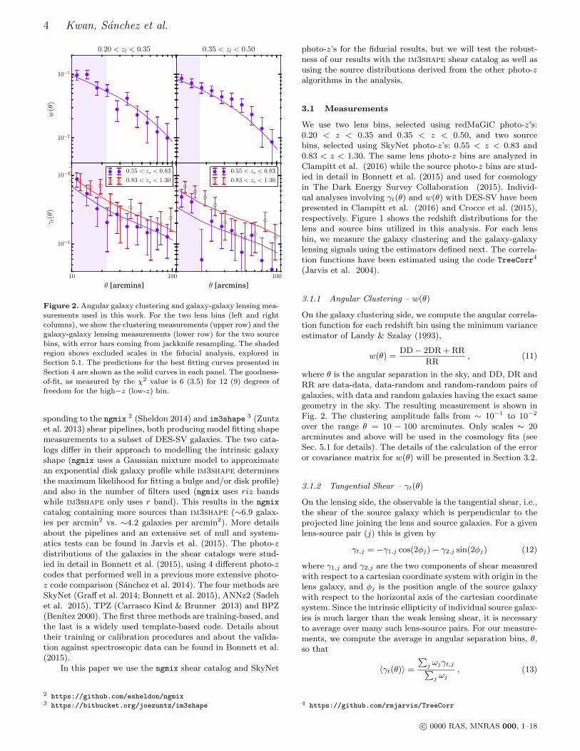
10−2
10−1
w(θ
)0.20 < zl < 0.35
101 102
0.35 < zl < 0.50
10 100
θ [arcmins]
10−4
10−3
γt(θ)
0.55 < zs < 0.83
0.83 < zs < 1.30
100
θ [arcmins]
0.55 < zs < 0.83
0.83 < zs < 1.30
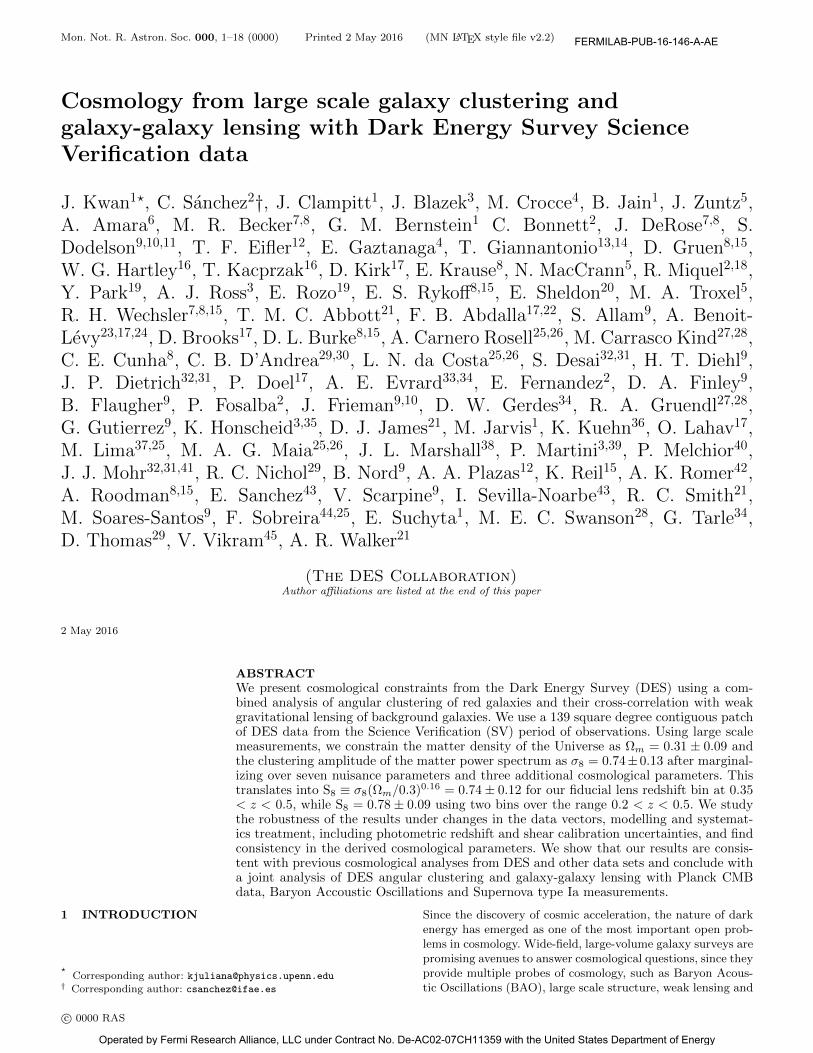
Figure 2. Angular galaxy clustering and galaxy-galaxy lensing mea-surements used in this work. For the two lens bins (left and right
columns), we show the clustering measurements (upper row) and the
galaxy-galaxy lensing measurements (lower row) for the two sourcebins, with error bars coming from jackknife resampling. The shaded
region shows excluded scales in the fiducial analysis, explored in
Section 5.1. The predictions for the best fitting curves presented inSection 4 are shown as the solid curves in each panel. The goodness-
of-fit, as measured by the χ2 value is 6 (3.5) for 12 (9) degrees of
freedom for the high−z (low-z) bin.
sponding to the ngmix 2 (Sheldon 2014) and im3shape 3 (Zuntzet al. 2013) shear pipelines, both producing model fitting shapemeasurements to a subset of DES-SV galaxies. The two cata-logs differ in their approach to modelling the intrinsic galaxyshape (ngmix uses a Gaussian mixture model to approximatean exponential disk galaxy profile while im3shape determinesthe maximum likelihood for fitting a bulge and/or disk profile)and also in the number of filters used (ngmix uses riz bandswhile im3shape only uses r band). This results in the ngmix
catalog containing more sources than im3shape (∼6.9 galax-ies per arcmin2 vs. ∼4.2 galaxies per arcmin2). More detailsabout the pipelines and an extensive set of null and system-atics tests can be found in Jarvis et al. (2015). The photo-zdistributions of the galaxies in the shear catalogs were stud-ied in detail in Bonnett et al. (2015), using 4 different photo-zcodes that performed well in a previous more extensive photo-z code comparison (Sanchez et al. 2014). The four methods areSkyNet (Graff et al. 2014; Bonnett et al. 2015), ANNz2 (Sadehet al. 2015), TPZ (Carrasco Kind & Brunner 2013) and BPZ(Benıtez 2000). The first three methods are training-based, andthe last is a widely used template-based code. Details abouttheir training or calibration procedures and about the valida-tion against spectroscopic data can be found in Bonnett et al.(2015).
In this paper we use the ngmix shear catalog and SkyNet
2 https://github.com/esheldon/ngmix3 https://bitbucket.org/joezuntz/im3shape
photo-z’s for the fiducial results, but we will test the robust-ness of our results with the im3shape shear catalog as well asusing the source distributions derived from the other photo-zalgorithms in the analysis.
3.1 Measurements
We use two lens bins, selected using redMaGiC photo-z’s:0.20 < z < 0.35 and 0.35 < z < 0.50, and two sourcebins, selected using SkyNet photo-z’s: 0.55 < z < 0.83 and0.83 < z < 1.30. The same lens photo-z bins are analyzed inClampitt et al. (2016) while the source photo-z bins are stud-ied in detail in Bonnett et al. (2015) and used for cosmologyin The Dark Energy Survey Collaboration (2015). Individ-ual analyses involving γt(θ) and w(θ) with DES-SV have beenpresented in Clampitt et al. (2016) and Crocce et al. (2015),respectively. Figure 1 shows the redshift distributions for thelens and source bins utilized in this analysis. For each lensbin, we measure the galaxy clustering and the galaxy-galaxylensing signals using the estimators defined next. The correla-tion functions have been estimated using the code TreeCorr4
(Jarvis et al. 2004).
3.1.1 Angular Clustering – w(θ)
On the galaxy clustering side, we compute the angular correla-tion function for each redshift bin using the minimum varianceestimator of Landy & Szalay (1993),
w(θ) =DD− 2DR + RR
RR, (11)
where θ is the angular separation in the sky, and DD, DR andRR are data-data, data-random and random-random pairs ofgalaxies, with data and random galaxies having the exact samegeometry in the sky. The resulting measurement is shown inFig. 2. The clustering amplitude falls from ∼ 10−1 to 10−2
over the range θ = 10 − 100 arcminutes. Only scales ∼ 20arcminutes and above will be used in the cosmology fits (seeSec. 5.1 for details). The details of the calculation of the erroror covariance matrix for w(θ) will be presented in Section 3.2.
3.1.2 Tangential Shear – γt(θ)
On the lensing side, the observable is the tangential shear, i.e.,the shear of the source galaxy which is perpendicular to theprojected line joining the lens and source galaxies. For a givenlens-source pair (j) this is given by
γt,j = −γ1,j cos(2φj)− γ2,j sin(2φj) (12)
where γ1,j and γ2,j are the two components of shear measuredwith respect to a cartesian coordinate system with origin in thelens galaxy, and φj is the position angle of the source galaxywith respect to the horizontal axis of the cartesian coordinatesystem. Since the intrinsic ellipticity of individual source galax-ies is much larger than the weak lensing shear, it is necessaryto average over many such lens-source pairs. For our measure-ments, we compute the average in angular separation bins, θ,so that
〈γt(θ)〉 =
∑j ωjγt,j∑j ωj
, (13)
4 https://github.com/rmjarvis/TreeCorr
c© 0000 RAS, MNRAS 000, 1–18
Cosmology from the Dark Energy Survey 5
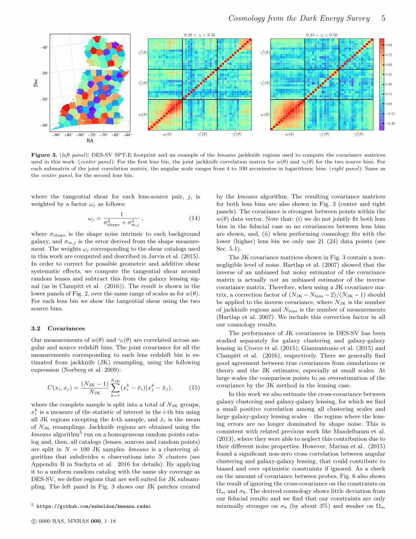
+60+65+70+75+80+85+90
RA
60
55
50
45
Dec
w() 1t () 2
t ()
w()
1t ()
2t ()
0.35 < zl < 0.50
0.30
0.15
0.00
0.15
0.30
0.45
0.60
0.75
0.90
w() 1t () 2
t ()
w()
1t ()
2t ()
0.20 < zl < 0.35
Figure 3. (left panel): DES-SV SPT-E footprint and an example of the kmeans jackknife regions used to compute the covariance matrices
used in this work. (center panel): For the first lens bin, the joint jackknife correlation matrix for w(θ) and γt(θ) for the two source bins. Foreach submatrix of the joint correlation matrix, the angular scale ranges from 4 to 100 arcminutes in logarithmic bins. (right panel): Same as
the center panel, for the second lens bin.
where the tangential shear for each lens-source pair, j, isweighted by a factor ωj as follows:
ωj =1
σ2shape + σ2
m,j
, (14)
where σshape is the shape noise intrinsic to each backgroundgalaxy, and σm,j is the error derived from the shape measure-ment. The weights ωj corresponding to the shear catalogs usedin this work are computed and described in Jarvis et al. (2015).In order to correct for possible geometric and additive shearsystematic effects, we compute the tangential shear aroundrandom lenses and subtract this from the galaxy lensing sig-nal (as in Clampitt et al. (2016)). The result is shown in thelower panels of Fig. 2, over the same range of scales as for w(θ).For each lens bin we show the tangential shear using the twosource bins.
3.2 Covariances
Our measurements of w(θ) and γt(θ) are correlated across an-gular and source redshift bins. The joint covariance for all themeasurements corresponding to each lens redshift bin is es-timated from jackknife (JK) resampling, using the followingexpression (Norberg et al. 2009):
C(xi, xj) =(NJK − 1)
NJK
NJK∑k=1
(xki − xi)(xkj − xj), (15)
where the complete sample is split into a total of NJK groups,xki is a measure of the statistic of interest in the i-th bin usingall JK regions excepting the k-th sample, and xi is the meanof NJK resamplings. Jackknife regions are obtained using thekmeans algorithm5 run on a homogeneous random points cata-log and, then, all catalogs (lenses, sources and random points)are split in N = 100 JK samples. kmeans is a clustering al-gorithm that subdivides n observations into N clusters (seeAppendix B in Suchyta et al. 2016 for details). By applyingit to a uniform random catalog with the same sky coverage asDES-SV, we define regions that are well suited for JK subsam-pling. The left panel in Fig. 3 shows our JK patches created
5 https://github.com/esheldon/kmeans radec
by the kmeans algorithm. The resulting covariance matricesfor both lens bins are also shown in Fig. 3 (center and rightpanels). The covariance is strongest between points within thew(θ) data vector. Note that: (i) we do not jointly fit both lensbins in the fiducial case so no covariances between lens binsare shown, and, (ii) when performing cosmology fits with thelower (higher) lens bin we only use 21 (24) data points (seeSec. 5.1).
The JK covariance matrices shown in Fig. 3 contain a non-negligible level of noise. Hartlap et al. (2007) showed that theinverse of an unbiased but noisy estimator of the covariancematrix is actually not an unbiased estimator of the inversecovariance matrix. Therefore, when using a JK covariance ma-trix, a correction factor of (NJK−Nbins− 2)/(NJK− 1) shouldbe applied to the inverse covariance, where NJK is the numberof jackknife regions and Nbins is the number of measurements(Hartlap et al. 2007). We include this correction factor in allour cosmology results.
The performance of JK covariances in DES-SV has beenstudied separately for galaxy clustering and galaxy-galaxylensing in Crocce et al. (2015); Giannantonio et al. (2015) andClampitt et al. (2016), respectively. There we generally findgood agreement between true covariances from simulations ortheory and the JK estimates, especially at small scales. Atlarge scales the comparison points to an overestimation of thecovariance by the JK method in the lensing case.
In this work we also estimate the cross-covariance betweengalaxy clustering and galaxy-galaxy lensing, for which we finda small positive correlation among all clustering scales andlarge galaxy-galaxy lensing scales – the regime where the lens-ing errors are no longer dominated by shape noise. This isconsistent with related previous work like Mandelbaum et al.(2013), where they were able to neglect this contribution due totheir different noise properties. However, Marian et al. (2015)found a significant non-zero cross correlation between angularclustering and galaxy-galaxy lensing, that could contribute tobiased and over optimistic constraints if ignored. As a checkon the amount of covariance between probes, Fig. 6 also showsthe result of ignoring the cross-covariance on the constraints onΩm and σ8. The derived cosmology shows little deviation fromour fiducial results and we find that our constraints are onlyminimally stronger on σ8 (by about 3%) and weaker on Ωm
c© 0000 RAS, MNRAS 000, 1–18
6 Kwan, Sanchez et al.
(also ∼3%) with a 2% improvement on S8 = σ8(Ωm/0.3)0.16.This shows that the impact of the correlation between probesis subdominant to the covariance within the same probe.
4 FIDUCIAL COSMOLOGICAL CONSTRAINTS
In this section we present our fiducial DES-SV cosmologicalconstraints from a joint analysis of clustering and galaxy-galaxy lensing. The data vector consists of w(θ) and the twoγt(θ) measurements for the 0.35 < z < 0.5 redMaGiC bin (seeFig. 2), over angular scales of 17-100 arcminutes. We chosethis lens bin as our fiducial, as we estimate greater contamina-tion from systematic errors, on both the clustering and lensingside, for the 0.2 < z < 0.35 redMaGiC bin (see Section 5.5 andClampitt et al. (2016)). To compute the model we use CAMB(Lewis et al. 2000; Howlett et al. 2012) and Halofit (Smith et al.2003; Takahashi et al. 2012) for the linear and non-linear mat-ter power spectra, respectively. Because the accuracy of Halofitcan be confirmed only to ∼5% for certain ΛCDM models, wehave checked that using the Cosmic Emulator, a more precisemodelling scheme for the nonlinear dark matter power spec-trum (1% to k = 1 Mpc−1, Lawrence et al. 2010) would onlyaffect our results at the level of ∼5% down to 10′. We use theCosmoSIS package6 (Zuntz et al. 2015) as our analysis pipelineand explore the joint posterior distribution of our cosmological(and nuisance) parameters using the multi-nest MCMC algo-rithm of Feroz et al (2009), with a tolerance parameter of 0.5and an efficiency parameter of 0.8. Our cosmological param-eters and priors are summarized in Table 1 and described ingreater detail next in this section.
In the fiducial case, we have included two nuisance param-eters per source bin (one for errors in the photo-z distributionand one for biases in the shear calibration) and one nuisanceparameter per lens bin (the linear bias, b1; the non-linear bias,b2, accounting for scale dependence and stochasticity, is stud-ied in Section 5.1), plus an additional term, α, to accountfor potential systematic errors induced by observational ef-fects that might induce an overall shift in the normalisationof the amplitude of w(θ) (see Section 5.5). The full set of nui-sance parameters and their priors are listed in the lower halfof Table 1 and summarized below.
• Photometric redshift calibration: For each source bini, we marginalize over a photo-z bias parameter, βi, definedsuch as ni(z) → ni (z + βi). In Bonnett et al. (2015), itwas found that a single additive parameter for the photo-zdistribution with a Gaussian prior centered on zero with adispersion of 0.05, was sufficient to account for any statisticalbias on Σcrit and hence σ8 within the degree of statisticalerror expected for the SV catalogs.• Shear calibration: For each source bin i, we marginal-ize over an extra nuisance parameter mi, to account forthe shear calibration uncertainties, such that γt;i(θ) →(1 +mi) γt;i(θ), with a Gaussian prior with mean 0 andwidth 0.05, as advocated in Jarvis et al. (2015).• Additive w(θ) constant: We marginalize over an addi-tive constant parameter, α, in the galaxy angular correla-tion function: w(θ)→ w(θ) + 10α. This parameter accountsfor possible systematics arising from variations in observing
6 https://bitbucket.org/joezuntz/cosmosis
conditions across the field, stellar contamination and mask-ing (Ross et al. 2011), which we also test for in the nextsection.
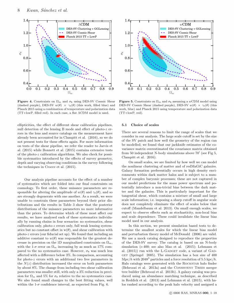
The resulting constraints in the Ωm and σ8 plane areshown in Fig. 4. The 2D contours are centered around Ωm ∼0.3 and σ8 ∼ 0.75, and marginalizing out the other parame-ter we find the following 1D constraints: Ωm = 0.31 ± 0.10and σ8 = 0.74 ± 0.13. Comparing to measurements fromPlanck (The Planck Collaboration et al. 2015) and DES Cos-mic Shear (The Dark Energy Survey Collaboration 2015)alone, we are consistent at the ∼ 1σ or better level. We com-bine results from the two experiments in Section 6. In addition,we see the same direction of degeneracy between these two pa-rameters as with cosmic shear, although the degeneracy is notquite as strong with w(θ) and γt(θ).
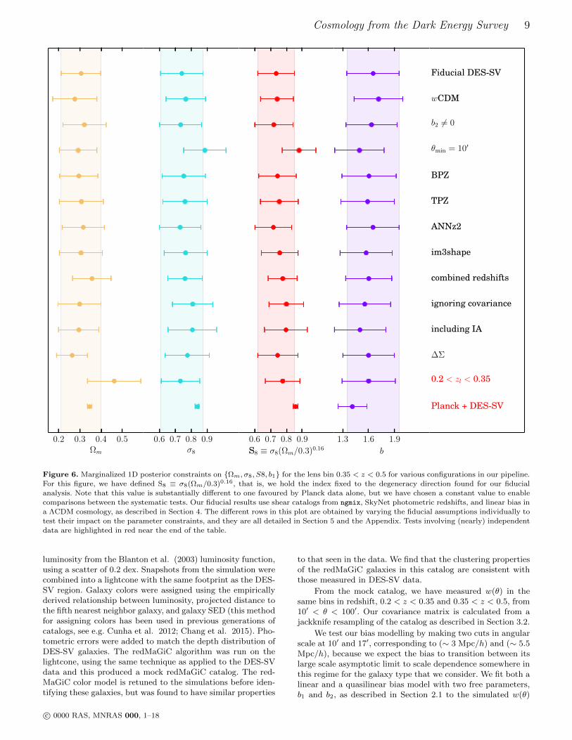
We also include w, the dark energy equation of state pa-rameter, as an additional free parameter in Fig. 5. We foundthat the DES-SV data alone was unable to provide strong con-straints on w and obtained w = −1.93± 1.16. However, com-pared to Planck (red contours), the DES-SV constraints onΩm and σ8 are degraded far less when w is introduced as afree parameter. Also, we note that the preference for w < −1values is determined by our choice of prior on w; we require−5 < w < −0.33, so the prior volume covered by w < −1 isgreater than w > −1 and in the absence of a strong constrainton w, values of w < −1 are favored.
Table 2 contains a more detailed summary of our findingsfor this fiducial setup, assuming either a ΛCDM or wCDMcosmology. In addition to DES w(θ) and γt(θ), we show re-sults combined with Planck. Table 2 also shows results forour lower redshift lens bin, 0.2 < z < 0.35. For these resultswe vary only the cosmological parameters Ωm,Ωb, h, ns, σ8and w where noted (in addition to the nuisance parameters de-scribed in the present and following sections). When combinedwith constraints from Planck, we also allow the optical depth,τ , to vary as well, since the CMB has additional sensitivity tophysics that is only weakly captured by large scale clusteringat late times. Table 3 shows the constraints on the nuisanceparameters related to photo-z and shear calibration describedabove.
In the following section, we will study the robustness ofthese results under changes in the configuration of the datavector and the systematics modelling.
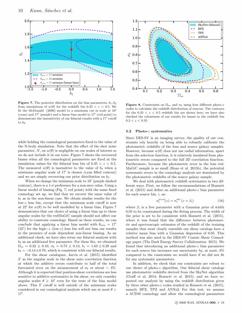
5 ROBUSTNESS OF THE RESULTS
In this section, we describe the suite of tests performed to checkthat our conclusions are unbiased with respect to errors in theshear and photo-z calibrations, intrinsic alignments, survey ge-ometry, choice of angular scales and theoretical modelling ofthe data vectors. The results in this section are displayed inFig. 6, for the parameters we are most sensitive to in thiswork: Ωm, σ8, b1. The different rows correspond to the dif-ferent tests described in this section or in the Appendix, wherewe check the results from a different lensing estimator. Despitethe changes in the photo-z algorithms, the shear catalogs, theweighting of the lens-source pairs, non-linear bias modellingand choice of scale, our estimates for these cosmological pa-rameters in Fig. 6 usually remain within 1-σ of the fiducialconstraints.
A number of systematics that are unique to the measure-ment of the tangential shear such as the calibration of galaxy
c© 0000 RAS, MNRAS 000, 1–18
Cosmology from the Dark Energy Survey 7
Parameter Prior range
Ωm 0.1 – 0.8 Normalized matter density
Ωb 0.04 – 0.05 Normalized baryon densityσ8 0.4 – 1.2 Amplitude of clustering (8 h−1Mpc top hat)
ns 0.85 – 1.05 Power spectrum tiltw -5 – -0.33 Equation of state parameter
h 0.5 – 1.0 Hubble parameter (H0 = 100h)
τ 0.04 – 0.12 Optical depth
b1 1.0 – 2.2 Linear galaxy biasb2 -1.5 – 1.5 Next order bias parameter
βi -0.3 – 0.3 Shift in photo-z distribution (per source bin)
mi -0.2 – 0.2 Shear multiplicative bias (per source bin)mIA -0.3 – 0.35 Intrinsic alignment amplitude (low-z source bin only)
α -5 – -1 Additive constant w(θ)→ w(θ) + 10α
Table 1. Parameters and their corresponding priors used in this work. Not all parameters are allowed to vary in every analysis. Nuisanceparameters are contained in the lower half of the table. When choosing a prior range on cosmological parameters, we allowed a sufficiently
wide range to contain all of the 2-σ posterior on Ωm, σ8, ns, w and h, with Planck priors on Ωb, for which we have less sensitivity. For the
systematic parameters, our choice of prior range is informed from previous DES analyses that studied the effect of shear calibration (Jarviset al. 2015), photo-z distributions (Bonnett et al. 2015), and intrinsic alignment contamination (Clampitt et al. 2016; The Dark Energy
Survey Collaboration 2015) on the SV catalogues. The prior on the bias parameters were taken from studies of the redMaGiC mock catalog
(see Section 5.1 for details). In addition to the prior range on the nuisance parameters for the shear calibration and photo-z bias, there is aGaussian prior centered around zero of width 0.5, as explained in the text.
Probes z σ8 Ωm S8 ≡ σ8(Ωm/0.3)α α b1 w0
DES 0.2 < z < 0.35 0.73 ± 0.12 0.46 ± 0.12 0.77 ± 0.11 0.15 1.60 ± 0.31 -1
DES 0.2 < z < 0.35 0.74 ± 0.13 0.41 ± 0.14 0.77 ± 0.10 0.17 1.73± 0.29 -2.5 ± 1.26DES 0.35 < z < 0.5 0.74 ± 0.13 0.31 ± 0.09 0.74 ± 0.12 0.16 1.64 ± 0.30 -1
DES 0.35 < z < 0.5 0.77 ± 0.12 0.28 ± 0.10 0.75 ± 0.11 0.13 1.71 ± 0.28 -2.03± 1.19
DES 0.2 < z < 0.5 0.76 ± 0.10 0.36 ± 0.09 0.78 ± 0.09 0.21 1.52 ± 0.28 -11.60 ± 0.27
Planck 0.83 ± 0.01 0.32 ± 0.01 0.82 ± 0.02 -0.49 -1
Planck 0.98+0.11−0.06 0.21+0.02
−0.07 1.21±0.27 -0.6 -1.54+0.20−0.40
BAO + SN + H0 0.33 ± 0.02 -1.07 ± 0.06
BAO + SN + H0 + DES 0.35 < z < 0.5 0.71±0.1 0.32 ± 0.02 0.71 ± 0.1 0.01 -1.05 ± 0.07DES + Planck 0.2 < z < 0.35 0.84 ± 0.01 0.35 ± 0.01 0.76 ± 0.02 -0.71 1.30 ± 0.13 -1
DES + Planck 0.2 < z < 0.35 0.89 ± 0.03 0.32 ± 0.02 0.84 ± 0.06 -0.76 1.25 ± 0.13 -1.16 ± 0.09
DES + Planck 0.35 < z < 0.5 0.84 ± 0.01 0.35 ± 0.01 0.76 ± 0.02 -0.71 1.41 ± 0.17 -1DES + Planck 0.35 < z < 0.5 0.88 ± 0.03 0.32 ± 0.02 0.84 ± 0.06 -0.75 1.36 ± 0.14 -1.14 ± 0.09
DES + Planck + 0.35 < z < 0.5 0.86 ± 0.02 0.31 ± 0.01 0.84 ± 0.03 -0.81 1.74 ± 0.28 -1.09 ± 0.05BAO + SN + H0
Table 2. Marginalized mean cosmological parameters (and 1-σ errors) measured from the posterior distribution of a joint analysis of angular
clustering and galaxy-galaxy lensing. Results for DES-SV data alone and in combination with Planck and external data (BAO, SN1a, H0) areshown for the two lens redshift bins both separately and combined. (Note that the biases are quoted separately: b1 = 1.52±0.28 for 0.2 < z <
0.35 and b1 = 1.60± 0.27 for 0.35 < z < 0.5). Not shown are the additional cosmological parameters that we have marginalized, ns,Ωb, h0as well as our standard set of nuisance parameters. Also quoted are the mean values and 1-σ errors given by Planck (TT+lowP) and externaldata alone.
Probes z 100β1 100β2 100m1 100m2 α
DES (ΛCDM) 0.2 < z < 0.35 −0.89± 4.58 0.25± 4.56 −0.09± 4.59 0.44± 4.42 -3.41 ± 0.84
DES (wCDM) 0.2 < z < 0.35 −1.00± 4.53 0.13± 4.51 −0.85± 4.47 0.14± 4.57 -3.42 ± 0.83
DES (ΛCDM) 0.35 < z < 0.5 −1.77± 4.46 0.14± 4.67 −0.05± 4.65 0.36± 4.64 -3.57 ± 0.81DES (wCDM) 0.35 < z < 0.5 −1.78± 4.38 0.18± 4.48 −0.85± 4.48 0.05± 4.31 -3.49 ± 0.81DES + Planck (ΛCDM) 0.2 < z < 0.35 −0.58± 4.83 0.29± 4.99 −0.63± 4.87 0.72± 4.84 -3.62 ± 0.82DES + Planck (wCDM) 0.2 < z < 0.35 −0.87± 4.73 0.14± 4.87 −0.76± 4.88 0.41± 4.79 -3.62 ± 0.82DES + Planck (ΛCDM) 0.35 < z < 0.5 −3.11± 4.48 −0.53± 4.95 −0.99± 4.92 −0.65± 4.77 -3.44 ± 0.87
DES + Planck (wCDM) 0.35 < z < 0.5 −1.04± 2.53 −0.16± 2.64 −1.09± 4.32 −0.68± 4.34 -3.43 ± 0.85
Table 3. Marginalized mean systematic uncertainty parameters with 1-σ errors measured from the posterior distribution of the joint analysisof angular clustering and galaxy-galaxy lensing in DES-SV data. We assume a Gaussian prior (centered on zero) for each systematic parameter,while the width of the prior is set from Jarvis et al. (2015) for the shear calibration and Bonnett et al. (2015) for the photo−zs. Each nuisance
parameter is additionally truncated by the amounts in Table 1.
c© 0000 RAS, MNRAS 000, 1–18
8 Kwan, Sanchez et al.
0.0 0.1 0.2 0.3 0.4 0.5 0.6 0.7 0.8 0.9Ωm
0.4
0.6
0.8
1.0
1.2
1.4σ
8
ΛCDMDES-SV Clustering + GGLensingDES-SV Cosmic ShearPlanck 2015 TT + LowP
Figure 4. Constraints on Ωm and σ8 using DES-SV Cosmic Shear(dashed purple), DES-SV w(θ) × γt(θ) (this work, filled blue) and
Planck 2015 using a combination of temperature and polarization data
(TT+lowP, filled red). In each case, a flat ΛCDM model is used.
0.0 0.1 0.2 0.3 0.4 0.5 0.6 0.7 0.8 0.9Ωm
0.4
0.6
0.8
1.0
1.2
1.4
σ8
wCDMDES-SV Clustering + GGLensingDES-SV Cosmic ShearPlanck 2015 TT + LowP
Figure 5. Constraints on Ωm and σ8 assuming a wCDM model usingDES-SV Cosmic Shear (dashed purple), DES-SV w(θ) × γt(θ) (this
work, blue) and Planck 2015 using temperature and polarization data
(TT+lowP, red).
ellipticities, the effect of different shear calibration pipelines,null detection of the lensing B mode and effect of photo-z er-rors in the lens and source catalogs on the measurement havealready been accounted for in Clampitt et al. (2016), so we donot present tests for these effects again. For more informationon tests of the shear pipeline, we refer the reader to Jarvis etal. (2015) while Bonnett et al. (2015) contains extensive testsof the photo-z calibration algorithms. We also check for possi-ble systematics introduced by the effects of survey geometry,depth and varying observing conditions in the survey followingthe techniques in Crocce et al. (2015).
Our analysis pipeline accounts for the effect of a numberof systematics which are folded into our final constraints oncosmology. To first order, these nuisance parameters are re-sponsible for altering the amplitude of w(θ) and γt(θ), and soare strongly degenerate with one another. As a result, we wereunable to constrain these parameters beyond their prior dis-tributions and the results in Table 3 show that the posteriordistributions of the nuisance parameters no more informativethan the priors. To determine which of these most affect ourresults, we have analysed each of these systematics individu-ally by running chains in four scenarios: no systematics, shearcalibration only, photo-z errors only, full weak lensing system-atics but no constant offset in w(θ), and shear calibration withphoto-z errors (our fiducial set up). We found that including anadditive constant to w(θ) was responsible for the greatest de-crease in precision on the 1D marginalized constraints on Ωm,with the 1-σ error on Ωm increasing by as much as 17% com-pared to the no systematics case. However, σ8 was much lessaffected with a difference below 3%. In comparison, accountingfor photo-z errors with an additional two free parameters inthe N(z) distribution increased the error on both parametersby about 8%. The change from including two shear calibrationparameters was smaller still, with only a 3% reduction in preci-sion for Ωm and 5% for σ8 relative to the no systematics case.We also found small changes to the best fitting values, wellwithin the 1-σ confidence interval, as expected from Fig. 6.
5.1 Choice of scales
There are several reasons to limit the range of scales that weconsider in our analysis. The large scale cutoff is set by the sizeof the SV patch and how well the geometry of the region canbe modelled; we found that our jackknife estimates of the co-variance matrix overestimated the covariance matrix obtainedfrom 50 independent N-body simulations above 70′ (see Fig 5,Clampitt et al. 2016).
On small scales, we are limited by how well we can modelthe nonlinear clustering of matter and of redMaGiC galaxies.Galaxy formation preferentially occurs in high density envi-ronments within dark matter halos and is subject to a num-ber of complex baryonic processes; these are not captured inour model predictions for the mass power spectrum and po-tentially introduce a non-trivial bias between the dark mat-ter and the galaxies. This is particularly important for thetangential shear, which contains a mixture of small and largescale information; i.e. imposing a sharp cutoff in angular scaledoes not completely eliminate the effect of scales below thatcutoff (Mandelbaum et al. 2013). On small enough scales, weexpect to observe effects such as stochasticity, non-local biasand scale dependence. These could invalidate the linear biasmodel used in our analysis.
In this section, we present simulation based tests to de-termine the smallest scales for which the linear bias modeland perturbation theory model of McDonald (2006) are valid.We use a mock catalog designed to reproduce the propertiesof the DES-SV survey. The catalog is based on an N-bodysimulation (c-400; see also Mao et al. (2015); Lehmann etal. (2015)) run with the L-Gadget code, a variant of Gad-get (Springel 2005). The simulation has a box size of 400Mpc/h with 20483 particles and a force resolution of 5.5 kpc/h.Halo catalogs were generated with the Rockstar halo finder(Behroozi et al. 2013a) and the Consistent Trees mergertree builder (Behroozi et al. 2013b). A galaxy catalog was pro-duced using an abundance matching technique, as describedin Reddick et al. (2013) and Lehmann et al. (2015), with ha-los ranked according to the peak halo velocity and assigned a
c© 0000 RAS, MNRAS 000, 1–18
Cosmology from the Dark Energy Survey 9
0.2 0.3 0.4 0.5Ωm
0.6 0.7 0.8 0.9σ8
0.6 0.7 0.8 0.9
S8 ≡ σ8(Ωm/0.3)0.16
1.3 1.6 1.9
b
Fiducial DES-SV
wCDM
b2 6= 0
θmin = 10′
BPZ
TPZ
ANNz2
im3shape
combined redshifts
ignoring covariance
including IA
∆Σ
0.2 < zl < 0.35
Planck + DES-SV
Figure 6. Marginalized 1D posterior constraints on Ωm, σ8, S8, b1 for the lens bin 0.35 < z < 0.5 for various configurations in our pipeline.
For this figure, we have defined S8 ≡ σ8(Ωm/0.3)0.16, that is, we hold the index fixed to the degeneracy direction found for our fiducialanalysis. Note that this value is substantially different to one favoured by Planck data alone, but we have chosen a constant value to enable
comparisons between the systematic tests. Our fiducial results use shear catalogs from ngmix, SkyNet photometric redshifts, and linear bias ina ΛCDM cosmology, as described in Section 4. The different rows in this plot are obtained by varying the fiducial assumptions individually totest their impact on the parameter constraints, and they are all detailed in Section 5 and the Appendix. Tests involving (nearly) independent
data are highlighted in red near the end of the table.
luminosity from the Blanton et al. (2003) luminosity function,using a scatter of 0.2 dex. Snapshots from the simulation werecombined into a lightcone with the same footprint as the DES-SV region. Galaxy colors were assigned using the empiricallyderived relationship between luminosity, projected distance tothe fifth nearest neighbor galaxy, and galaxy SED (this methodfor assigning colors has been used in previous generations ofcatalogs, see e.g. Cunha et al. 2012; Chang et al. 2015). Pho-tometric errors were added to match the depth distribution ofDES-SV galaxies. The redMaGiC algorithm was run on thelightcone, using the same technique as applied to the DES-SVdata and this produced a mock redMaGiC catalog. The red-MaGiC color model is retuned to the simulations before iden-tifying these galaxies, but was found to have similar properties
to that seen in the data. We find that the clustering propertiesof the redMaGiC galaxies in this catalog are consistent withthose measured in DES-SV data.
From the mock catalog, we have measured w(θ) in thesame bins in redshift, 0.2 < z < 0.35 and 0.35 < z < 0.5, from10′ < θ < 100′. Our covariance matrix is calculated from ajackknife resampling of the catalog as described in Section 3.2.
We test our bias modelling by making two cuts in angularscale at 10′ and 17′, corresponding to (∼ 3 Mpc/h) and (∼ 5.5Mpc/h), because we expect the bias to transition between itslarge scale asymptotic limit to scale dependence somewhere inthis regime for the galaxy type that we consider. We fit both alinear and a quasilinear bias model with two free parameters,b1 and b2, as described in Section 2.1 to the simulated w(θ)
c© 0000 RAS, MNRAS 000, 1–18
10 Kwan, Sanchez et al.
-1.5 -1.0 -0.5 0.0 0.5 1.0 1.5b2
1.0
1.2
1.4
1.6
1.8
2.0b 1
θmin = 17 arcminsθmin = 10 arcminsθmin = 17 arcmins (linear bias)
Figure 7. The posterior distribution on the bias parameters, b1, b2from simulations of w(θ) for the redshift bin 0.35 < z < 0.5. Wefit the McDonald (2006) model to a minimum cut in scale at 10′
(cyan) and 17′ (purple) and a linear bias model to 17′ (red point) todemonstrate the insensitivity of our fiducial results with a 17′ cutoff
to b2.
while holding the cosmological parameters fixed to the value ofthe N-body simulation. Note that the effect of the shot noiseparameter, N , on w(θ) is negligible on our scales of interest sowe do not include it in our tests. Figure 7 shows the recoveredbiases when all the cosmological parameters are fixed at thesimulation values for the fiducial lens bin of 0.35 < z < 0.5.The measured w(θ) is insensitive to the value of b2 when aminimum angular scale of 17′ is chosen (cyan filled contour)and we are simply recovering our prior distribution on b2.
When we change the minimum scale to 10′ (purple dashedcontour), there is a 1-σ preference for a non-zero value. Using alinear model of biasing (Fig. 7; red point) with the same fixedcosmology set up, we find that we recover the same value ofb1 as in the non-linear case. We obtain similar results for thelow-z lens bin, except that the minimum scale cutoff is nowat 22′ for w(θ) to be well modelled by a linear bias. Figure 7demonstrates that our choice of using a linear bias up to theseangular scales for the redMaGiC sample should not affect ourability to constrain cosmology. Based on these results, we canconclude that applying a linear bias model with θmin = 17′
(22′) for the high−z (low-z) lens bin will not bias our resultsin the presence of scale dependent non-linear biasing. As anadditional check, we have also rerun our fiducial analysis withb2 as an additional free parameter. For these fits, we obtainedΩm = 0.32 ± 0.10, σ8 = 0.73 ± 0.13, b1 = 1.63 ± 0.29 andb2 = −0.14±0.76, which is consistent with our fiducial results.
For the shear catalogues, Jarvis et al. (2015) identified3′ as the angular scale in the shear auto correlation functionat which the additive errors contribute to half of the totalforecasted error on the measurement of σ8 or about ∼ 3%.Although it is expected that position-shear correlations are lesssensitive to additive systematics in the shear, we only considerangular scales θ > 10′ even for the tests of the bias modelabove. This 3′ cutoff is well outside of the minimum scalesconsidered in our cosmological analysis which use at most θ >17′.
0.1 0.2 0.3 0.4 0.5 0.6Ωm
0.4
0.5
0.6
0.7
0.8
0.9
1.0
1.1
1.2
σ8
SkyNet (fiducial)BPZTPZANNz2
Figure 8. Constraints on Ωm and σ8 using four different photo-z
codes to calculate the redshift distribution of sources. The contoursfor the 0.35 < z < 0.5 redshift bin are shown here; we have also
checked the robustness of our results for lenses in the redshift bin
0.2 < z < 0.35.
5.2 Photo-z systematics
Since DES-SV is an imaging survey, the quality of our con-straints rely heavily on being able to robustly calibrate thephotometric redshifts of the lens and source galaxy samples.However, because w(θ) does not use radial information, apartfrom the selection function, it is relatively insulated from pho-tometric errors compared to the full 3D correlation function.Furthermore, because the photometric error in the lens red-MaGiC sample is so small (Rozo et al. 2015b), the potentialsystematic errors in the cosmology analysis are dominated bythe photometric redshifts of the source galaxy sample.
We deal with photometric redshift systematics in two dif-ferent ways. First, we follow the recommendations of Bonnettet al. (2015) and define an additional photo-z bias parameterfor each source bin, i, as:
npredi (z) = nobsi (z + βi) (16)
where βi is a free parameter with a Gaussian prior of width0.05 to be constrained during the fitting process. The width ofthe prior is set to be consistent with Bonnett et al. (2015),where it was found that the difference between photomet-ric and spectroscopic estimates of the redshift of the trainingsamples that most closely resemble our shear catalogs have arelative mean bias with a Gaussian dispersion of 0.05. Thismethod was also used in the DES-SV Cosmic Shear Cosmol-ogy paper (The Dark Energy Survey Collaboration 2015). Wefound that introducing an additional photo-z bias parameterfor each source bin increases our uncertainty by, at most, 8%compared to the constraints we would have if we did not fitfor any systematic parameters.
In addition, we check that our constraints are robust toour choice of photo-z algorithm. Our fiducial shear catalogsuse photometric redshifts derived from the SkyNet algorithm(Graff et al. 2014; Bonnett et al. 2015), and we have re-peated our analysis by using the redshift distribution givenby three other photo-z codes studied in Bonnett et al. (2015),namely BPZ, TPZ and ANNz2. For this test, we assumea ΛCDM cosmology and allow the cosmological parameters
c© 0000 RAS, MNRAS 000, 1–18
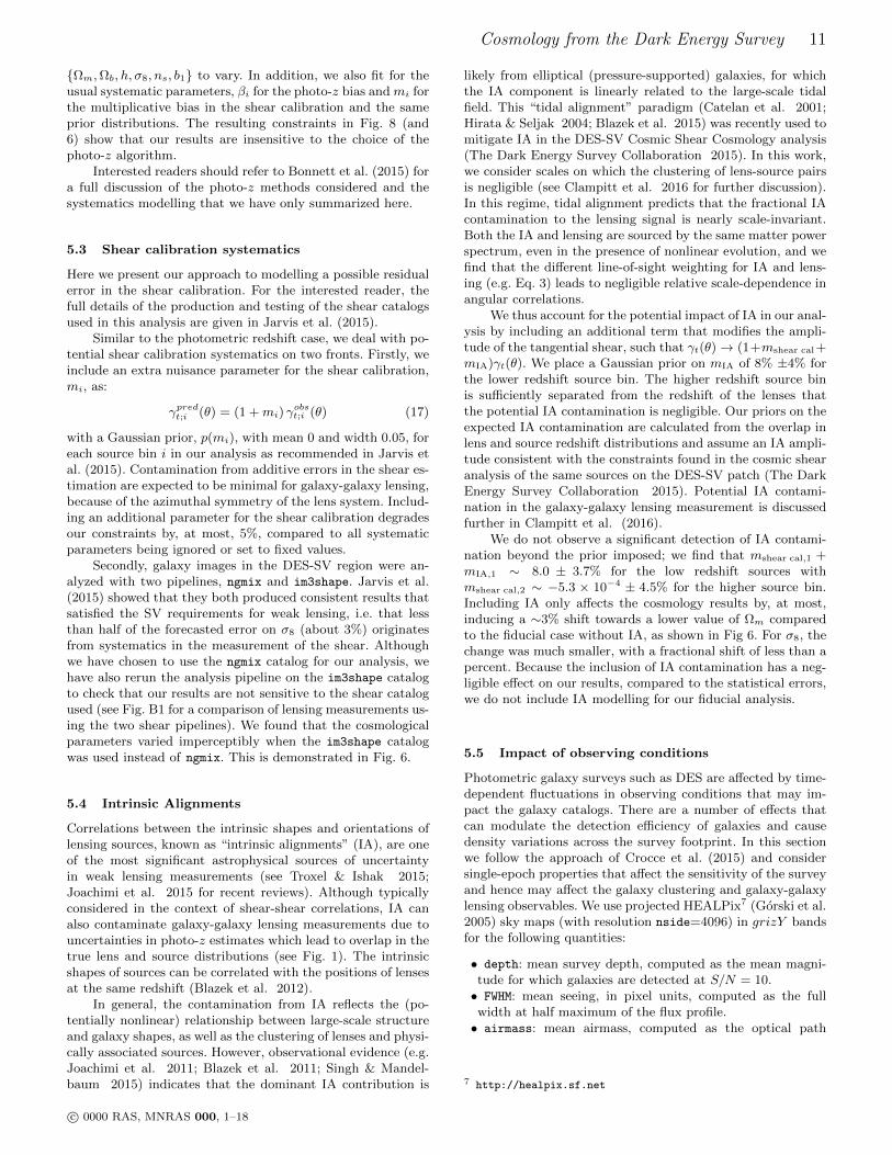
Cosmology from the Dark Energy Survey 11
Ωm,Ωb, h, σ8, ns, b1 to vary. In addition, we also fit for theusual systematic parameters, βi for the photo-z bias and mi forthe multiplicative bias in the shear calibration and the sameprior distributions. The resulting constraints in Fig. 8 (and6) show that our results are insensitive to the choice of thephoto-z algorithm.
Interested readers should refer to Bonnett et al. (2015) fora full discussion of the photo-z methods considered and thesystematics modelling that we have only summarized here.
5.3 Shear calibration systematics
Here we present our approach to modelling a possible residualerror in the shear calibration. For the interested reader, thefull details of the production and testing of the shear catalogsused in this analysis are given in Jarvis et al. (2015).
Similar to the photometric redshift case, we deal with po-tential shear calibration systematics on two fronts. Firstly, weinclude an extra nuisance parameter for the shear calibration,mi, as:
γpredt;i (θ) = (1 +mi) γobst;i (θ) (17)
with a Gaussian prior, p(mi), with mean 0 and width 0.05, foreach source bin i in our analysis as recommended in Jarvis etal. (2015). Contamination from additive errors in the shear es-timation are expected to be minimal for galaxy-galaxy lensing,because of the azimuthal symmetry of the lens system. Includ-ing an additional parameter for the shear calibration degradesour constraints by, at most, 5%, compared to all systematicparameters being ignored or set to fixed values.
Secondly, galaxy images in the DES-SV region were an-alyzed with two pipelines, ngmix and im3shape. Jarvis et al.(2015) showed that they both produced consistent results thatsatisfied the SV requirements for weak lensing, i.e. that lessthan half of the forecasted error on σ8 (about 3%) originatesfrom systematics in the measurement of the shear. Althoughwe have chosen to use the ngmix catalog for our analysis, wehave also rerun the analysis pipeline on the im3shape catalogto check that our results are not sensitive to the shear catalogused (see Fig. B1 for a comparison of lensing measurements us-ing the two shear pipelines). We found that the cosmologicalparameters varied imperceptibly when the im3shape catalogwas used instead of ngmix. This is demonstrated in Fig. 6.
5.4 Intrinsic Alignments
Correlations between the intrinsic shapes and orientations oflensing sources, known as “intrinsic alignments” (IA), are oneof the most significant astrophysical sources of uncertaintyin weak lensing measurements (see Troxel & Ishak 2015;Joachimi et al. 2015 for recent reviews). Although typicallyconsidered in the context of shear-shear correlations, IA canalso contaminate galaxy-galaxy lensing measurements due touncertainties in photo-z estimates which lead to overlap in thetrue lens and source distributions (see Fig. 1). The intrinsicshapes of sources can be correlated with the positions of lensesat the same redshift (Blazek et al. 2012).
In general, the contamination from IA reflects the (po-tentially nonlinear) relationship between large-scale structureand galaxy shapes, as well as the clustering of lenses and physi-cally associated sources. However, observational evidence (e.g.Joachimi et al. 2011; Blazek et al. 2011; Singh & Mandel-baum 2015) indicates that the dominant IA contribution is
likely from elliptical (pressure-supported) galaxies, for whichthe IA component is linearly related to the large-scale tidalfield. This “tidal alignment” paradigm (Catelan et al. 2001;Hirata & Seljak 2004; Blazek et al. 2015) was recently used tomitigate IA in the DES-SV Cosmic Shear Cosmology analysis(The Dark Energy Survey Collaboration 2015). In this work,we consider scales on which the clustering of lens-source pairsis negligible (see Clampitt et al. 2016 for further discussion).In this regime, tidal alignment predicts that the fractional IAcontamination to the lensing signal is nearly scale-invariant.Both the IA and lensing are sourced by the same matter powerspectrum, even in the presence of nonlinear evolution, and wefind that the different line-of-sight weighting for IA and lens-ing (e.g. Eq. 3) leads to negligible relative scale-dependence inangular correlations.
We thus account for the potential impact of IA in our anal-ysis by including an additional term that modifies the ampli-tude of the tangential shear, such that γt(θ)→ (1+mshear cal+mIA)γt(θ). We place a Gaussian prior on mIA of 8% ±4% forthe lower redshift source bin. The higher redshift source binis sufficiently separated from the redshift of the lenses thatthe potential IA contamination is negligible. Our priors on theexpected IA contamination are calculated from the overlap inlens and source redshift distributions and assume an IA ampli-tude consistent with the constraints found in the cosmic shearanalysis of the same sources on the DES-SV patch (The DarkEnergy Survey Collaboration 2015). Potential IA contami-nation in the galaxy-galaxy lensing measurement is discussedfurther in Clampitt et al. (2016).
We do not observe a significant detection of IA contami-nation beyond the prior imposed; we find that mshear cal,1 +mIA,1 ∼ 8.0 ± 3.7% for the low redshift sources withmshear cal,2 ∼ −5.3 × 10⁻⁴ ± 4.5% for the higher source bin.Including IA only affects the cosmology results by, at most,inducing a ∼3% shift towards a lower value of Ωm comparedto the fiducial case without IA, as shown in Fig 6. For σ8, thechange was much smaller, with a fractional shift of less than apercent. Because the inclusion of IA contamination has a neg-ligible effect on our results, compared to the statistical errors,we do not include IA modelling for our fiducial analysis.
5.5 Impact of observing conditions
Photometric galaxy surveys such as DES are affected by time-dependent fluctuations in observing conditions that may im-pact the galaxy catalogs. There are a number of effects thatcan modulate the detection efficiency of galaxies and causedensity variations across the survey footprint. In this sectionwe follow the approach of Crocce et al. (2015) and considersingle-epoch properties that affect the sensitivity of the surveyand hence may affect the galaxy clustering and galaxy-galaxylensing observables. We use projected HEALPix7 (Gorski et al.2005) sky maps (with resolution nside=4096) in grizY bandsfor the following quantities:
• depth: mean survey depth, computed as the mean magni-tude for which galaxies are detected at S/N = 10.• FWHM: mean seeing, in pixel units, computed as the fullwidth at half maximum of the flux profile.• airmass: mean airmass, computed as the optical path
7 http://healpix.sf.net
c© 0000 RAS, MNRAS 000, 1–18
12 Kwan, Sanchez et al.
0.4
0.6
0.8
1.0
1.2
1.4
ngal/ngal
g band
0.20 < zl < 0.35
UncorrectedCorrected
0.35 < zl < 0.50
0.4
0.6
0.8
1.0
1.2
1.4
ngal/ngal
r band
1.1 1.2 1.3 1.4 1.5
airmass
0.4
0.6
0.8
1.0
1.2
1.4
ngal/ngal
i band
1.1 1.2 1.3 1.4 1.5
airmass
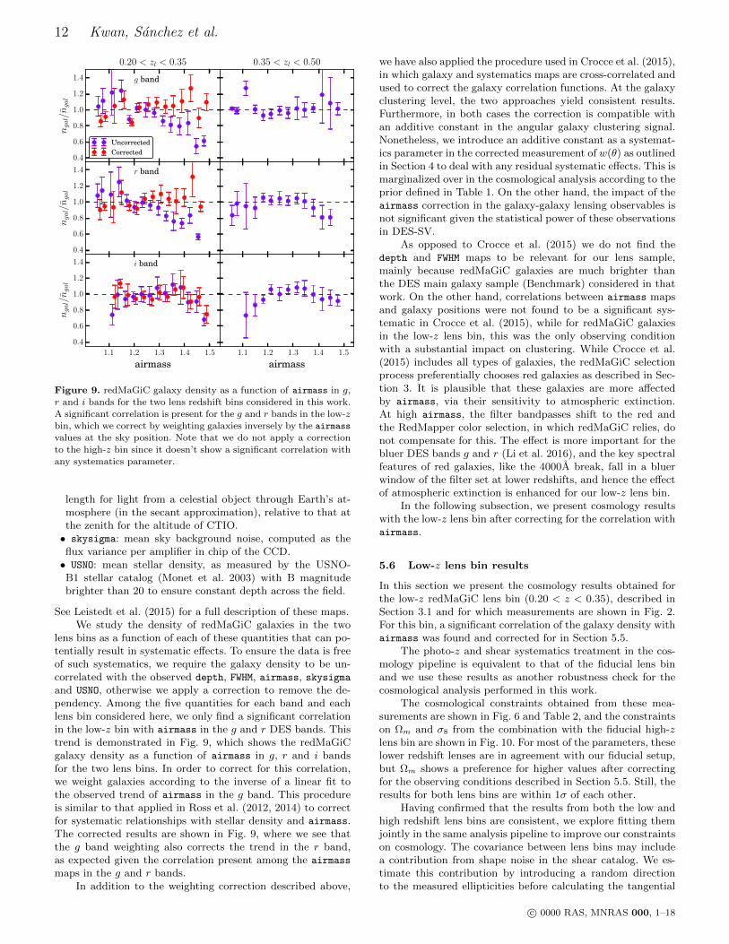
Figure 9. redMaGiC galaxy density as a function of airmass in g,
r and i bands for the two lens redshift bins considered in this work.A significant correlation is present for the g and r bands in the low-z
bin, which we correct by weighting galaxies inversely by the airmass
values at the sky position. Note that we do not apply a correction
to the high-z bin since it doesn’t show a significant correlation with
any systematics parameter.
length for light from a celestial object through Earth’s at-mosphere (in the secant approximation), relative to that atthe zenith for the altitude of CTIO.• skysigma: mean sky background noise, computed as theflux variance per amplifier in chip of the CCD.• USNO: mean stellar density, as measured by the USNO-B1 stellar catalog (Monet et al. 2003) with B magnitudebrighter than 20 to ensure constant depth across the field.
See Leistedt et al. (2015) for a full description of these maps.We study the density of redMaGiC galaxies in the two
lens bins as a function of each of these quantities that can po-tentially result in systematic effects. To ensure the data is freeof such systematics, we require the galaxy density to be un-correlated with the observed depth, FWHM, airmass, skysigmaand USNO, otherwise we apply a correction to remove the de-pendency. Among the five quantities for each band and eachlens bin considered here, we only find a significant correlationin the low-z bin with airmass in the g and r DES bands. Thistrend is demonstrated in Fig. 9, which shows the redMaGiCgalaxy density as a function of airmass in g, r and i bandsfor the two lens bins. In order to correct for this correlation,we weight galaxies according to the inverse of a linear fit tothe observed trend of airmass in the g band. This procedureis similar to that applied in Ross et al. (2012, 2014) to correctfor systematic relationships with stellar density and airmass.The corrected results are shown in Fig. 9, where we see thatthe g band weighting also corrects the trend in the r band,as expected given the correlation present among the airmass
maps in the g and r bands.In addition to the weighting correction described above,
we have also applied the procedure used in Crocce et al. (2015),in which galaxy and systematics maps are cross-correlated andused to correct the galaxy correlation functions. At the galaxyclustering level, the two approaches yield consistent results.Furthermore, in both cases the correction is compatible withan additive constant in the angular galaxy clustering signal.Nonetheless, we introduce an additive constant as a systemat-ics parameter in the corrected measurement of w(θ) as outlinedin Section 4 to deal with any residual systematic effects. This ismarginalized over in the cosmological analysis according to theprior defined in Table 1. On the other hand, the impact of theairmass correction in the galaxy-galaxy lensing observables isnot significant given the statistical power of these observationsin DES-SV.
As opposed to Crocce et al. (2015) we do not find thedepth and FWHM maps to be relevant for our lens sample,mainly because redMaGiC galaxies are much brighter thanthe DES main galaxy sample (Benchmark) considered in thatwork. On the other hand, correlations between airmass mapsand galaxy positions were not found to be a significant sys-tematic in Crocce et al. (2015), while for redMaGiC galaxiesin the low-z lens bin, this was the only observing conditionwith a substantial impact on clustering. While Crocce et al.(2015) includes all types of galaxies, the redMaGiC selectionprocess preferentially chooses red galaxies as described in Sec-tion 3. It is plausible that these galaxies are more affectedby airmass, via their sensitivity to atmospheric extinction.At high airmass, the filter bandpasses shift to the red andthe RedMapper color selection, in which redMaGiC relies, donot compensate for this. The effect is more important for thebluer DES bands g and r (Li et al. 2016), and the key spectralfeatures of red galaxies, like the 4000A break, fall in a bluerwindow of the filter set at lower redshifts, and hence the effectof atmospheric extinction is enhanced for our low-z lens bin.
In the following subsection, we present cosmology resultswith the low-z lens bin after correcting for the correlation withairmass.
5.6 Low-z lens bin results
In this section we present the cosmology results obtained forthe low-z redMaGiC lens bin (0.20 < z < 0.35), described inSection 3.1 and for which measurements are shown in Fig. 2.For this bin, a significant correlation of the galaxy density withairmass was found and corrected for in Section 5.5.
The photo-z and shear systematics treatment in the cos-mology pipeline is equivalent to that of the fiducial lens binand we use these results as another robustness check for thecosmological analysis performed in this work.
The cosmological constraints obtained from these mea-surements are shown in Fig. 6 and Table 2, and the constraintson Ωm and σ8 from the combination with the fiducial high-zlens bin are shown in Fig. 10. For most of the parameters, theselower redshift lenses are in agreement with our fiducial setup,but Ωm shows a preference for higher values after correctingfor the observing conditions described in Section 5.5. Still, theresults for both lens bins are within 1σ of each other.
Having confirmed that the results from both the low andhigh redshift lens bins are consistent, we explore fitting themjointly in the same analysis pipeline to improve our constraintson cosmology. The covariance between lens bins may includea contribution from shape noise in the shear catalog. We es-timate this contribution by introducing a random directionto the measured ellipticities before calculating the tangential
c© 0000 RAS, MNRAS 000, 1–18
Cosmology from the Dark Energy Survey 13
0.1 0.2 0.3 0.4 0.5 0.6 0.7 0.8 0.9Ωm
0.4
0.5
0.6
0.7
0.8
0.9
1.0
1.1
1.2σ
8
0.35 < zl < 0.50
0.20 < zl < 0.35
Combined
Figure 10. Constraints on Ωm and σ8 using DES-SV w(θ) × γt(θ).
The fiducial high-z lens bin is shown in filled blue, the low-z lens
bin is shown as dashed purple lines and the combination of the twolens bins is shown in filled red. In each case, a flat ΛCDM model is
assumed.
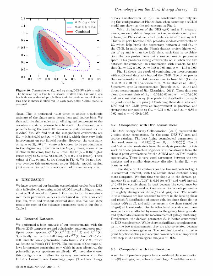
shear. This is performed ∼300 times to obtain a jackknifeestimate of the shape noise across lens and source bins. Wethen add the shape noise as an off-diagonal component to thecovariance matrix between lens bins with the diagonal com-ponents being the usual JK covariance matrices used for in-dividual fits. We find that the marginalized constraints areΩm = 0.36± 0.09 and σ8 = 0.76± 0.11, which show very littleimprovement on our fiducial results. However, the constrainton S8 ≡ σ8(Ωm/0.3)α, where α is chosen to be perpendicularto the degeneracy direction in the Ωm-σ8 plane, shows a re-duction in the error, from S8 = 0.735±0.117 (α = 0.16; high-zlenses only) to S8 = 0.782± 0.088 (α = 0.21; all lenses). Thesevalues of Ωm, σ8 and S8 are shown in Fig. 6. We do not how-ever consider this arrangement as our ‘fiducial’ model, leavingjoint constraints to future work with additional survey area.
6 DISCUSSION
We have presented our baseline cosmological results from DESdata in Section 4, assuming a flat ΛCDM model in Figure 4 anda flat wCDM model in Figure 5. Our results for the marginal-ized mean parameter values are contained in Table 2 for eachlens bin, with and without external data sets. We also showresults for each of the nuisance parameters used in our fits inTable 3.
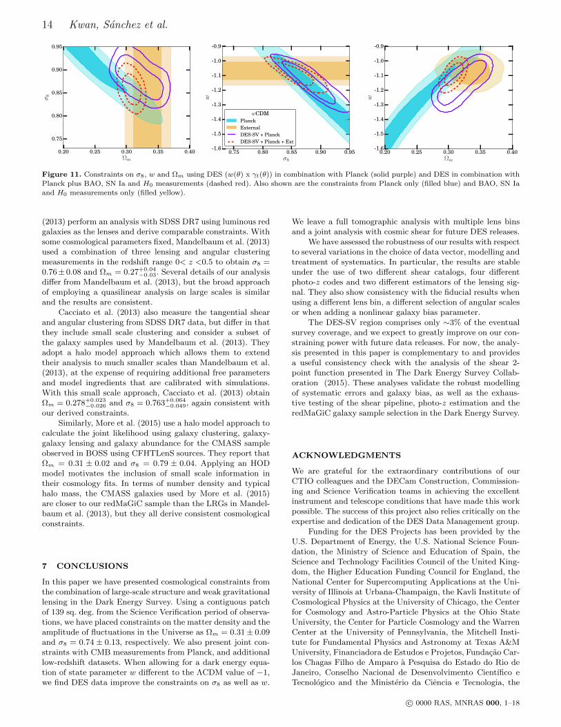
6.1 External Datasets
We performed a joint analysis of our measurements with thePlanck 2015 temperature and polarization auto and cross mul-tipole power spectra, CTT (`), CTE(`), CEE(`) and CBB(`).Specifically, we use the full range of CTT (`) from 29 < ` <2509 and the low-` polarization data from 2 < ` < 29, whichwe denote as Planck (TT-lowP). The inclusion of the maps al-lows for stronger constraints on τ which in turn affects As, theprimordial power spectrum amplitude. We have also chosenthis configuration to allow for an easy comparison with theDES-SV Cosmic Shear Cosmology paper (The Dark Energy
Survey Collaboration 2015). The constraints from only us-ing this configuration of Planck data when assuming a wCDMmodel are shown as the red contours in Fig. 5.
With the inclusion of the DES γt(θ) and w(θ) measure-ments, we were able to improve on the constraints on σ8 andw from just Planck alone, which prefers w ≈ −1.5 and σ8 ≈ 1.This is in part because DES provides modest constraints onH0 which help break the degeneracy between h and Ωm inthe CMB. In addition, the Planck dataset prefers higher val-ues of σ8 and h than the DES data, such that in combina-tion, the two probes carve out a smaller area in parameterspace. This produces strong constraints on w when the twodatasets are combined. In combination with Planck, we findthat Ωm = 0.32±0.02, σ8 = 0.88±0.03 and w = −1.15±0.09.
Fig. 11 shows the result of combining our measurementswith additional data sets beyond the CMB. The other probesthat we consider are BAO measurements from 6dF (Beutleret al. 2011), BOSS (Anderson et al. 2014; Ross et al. 2015),Supernova type Ia measurements (Betoule et al. 2014) anddirect measurements of H0 (Efstathiou, 2014). These data setsalone give constraints of Ωm = 0.33±0.02 and w = −1.07±0.06and no constraint on σ8 (the posterior distribution on σ8 isfully informed by the prior). Combining these data sets withDES and the CMB gives an improvement in precision andstrengthens our results to Ωm = 0.31 ± 0.01 and σ8 = 0.86 ±0.02 and w = −1.09± 0.05.
6.2 Comparison with DES cosmic shear
The Dark Energy Survey Collaboration (2015) measured the2-point shear correlations, for the same DES-SV area andsource catalogs. The best fitting cosmological parameters inthat work were σ8 = 0.81+0.16
−0.26 and Ωm = 0.36+0.09−0.21. Figs. 4
and 5 show the constraints from the analysis presented in thiswork on those parameters together with constraints from theshear 2-point correlations for the ΛCDM and wCDM models,respectively. There is very good agreement between the twoanalyses and a similar degeneracy direction in the Ωm – σ8
plane as well.The shape of the contours for the two methods in Fig. 4
is somewhat different, with the cosmic shear contours beingmore elongated. We find that the slope α in the derived pa-rameter S8 ≡ σ8(Ωm/0.3)α is 0.16 for w(θ) and γt(θ) insteadof 0.478 for cosmic shear. In part because the covariance be-tween Ωm and σ8 is weaker, the constraints on each parameterare slightly stronger for the w(θ) and γt(θ) case. The resultsin this analysis are less sensitive to errors in the lensing shearand redshift distribution of source galaxies since these do notimpact w(θ) at all, and additive errors in the shear cancel outof γt(θ) at lowest order. On the other hand, cosmic shear mea-surements are unaffected by errors in the galaxy biasing modeland systematic errors in the measurement of galaxy clustering.Furthermore, the derived parameter S8 is better constrainedby DES cosmic shear. While there is significant complementar-ity in the two measurements, they are also correlated becauseof the shared source galaxies. The combination of all three 2-point functions taking into account covariances is an importantnext step in the cosmological analysis of DES.
6.3 Comparison with the literature
A number of previous papers have considered the combinationof w(θ) and γt(θ) as probes of cosmology. Mandelbaum et al.
c© 0000 RAS, MNRAS 000, 1–18
14 Kwan, Sanchez et al.
0.20 0.25 0.30 0.35 0.40Ωm
0.75
0.80
0.85
0.90
0.95σ
8
0.75 0.80 0.85 0.90 0.95σ8
-1.6
-1.5
-1.4
-1.3
-1.2
-1.1
-1.0
-0.9
w
wCDMPlanckExternalDES-SV + PlanckDES-SV + Planck + Ext
0.20 0.25 0.30 0.35 0.40Ωm
-1.6
-1.5
-1.4
-1.3
-1.2
-1.1
-1.0
-0.9
w
Figure 11. Constraints on σ8, w and Ωm using DES (w(θ) x γt(θ)) in combination with Planck (solid purple) and DES in combination with
Planck plus BAO, SN Ia and H0 measurements (dashed red). Also shown are the constraints from Planck only (filled blue) and BAO, SN Ia
and H0 measurements only (filled yellow).
(2013) perform an analysis with SDSS DR7 using luminous redgalaxies as the lenses and derive comparable constraints. Withsome cosmological parameters fixed, Mandelbaum et al. (2013)used a combination of three lensing and angular clusteringmeasurements in the redshift range 0< z <0.5 to obtain σ8 =0.76±0.08 and Ωm = 0.27+0.04
−0.03. Several details of our analysisdiffer from Mandelbaum et al. (2013), but the broad approachof employing a quasilinear analysis on large scales is similarand the results are consistent.
Cacciato et al. (2013) also measure the tangential shearand angular clustering from SDSS DR7 data, but differ in thatthey include small scale clustering and consider a subset ofthe galaxy samples used by Mandelbaum et al. (2013). Theyadopt a halo model approach which allows them to extendtheir analysis to much smaller scales than Mandelbaum et al.(2013), at the expense of requiring additional free parametersand model ingredients that are calibrated with simulations.With this small scale approach, Cacciato et al. (2013) obtainΩm = 0.278+0.023
−0.026 and σ8 = 0.763+0.064−0.049, again consistent with
our derived constraints.Similarly, More et al. (2015) use a halo model approach to
calculate the joint likelihood using galaxy clustering, galaxy-galaxy lensing and galaxy abundance for the CMASS sampleobserved in BOSS using CFHTLenS sources. They report thatΩm = 0.31 ± 0.02 and σ8 = 0.79 ± 0.04. Applying an HODmodel motivates the inclusion of small scale information intheir cosmology fits. In terms of number density and typicalhalo mass, the CMASS galaxies used by More et al. (2015)are closer to our redMaGiC sample than the LRGs in Mandel-baum et al. (2013), but they all derive consistent cosmologicalconstraints.
7 CONCLUSIONS
In this paper we have presented cosmological constraints fromthe combination of large-scale structure and weak gravitationallensing in the Dark Energy Survey. Using a contiguous patchof 139 sq. deg. from the Science Verification period of observa-tions, we have placed constraints on the matter density and theamplitude of fluctuations in the Universe as Ωm = 0.31± 0.09and σ8 = 0.74 ± 0.13, respectively. We also present joint con-straints with CMB measurements from Planck, and additionallow-redshift datasets. When allowing for a dark energy equa-tion of state parameter w different to the ΛCDM value of −1,we find DES data improve the constraints on σ8 as well as w.
We leave a full tomographic analysis with multiple lens binsand a joint analysis with cosmic shear for future DES releases.
We have assessed the robustness of our results with respectto several variations in the choice of data vector, modelling andtreatment of systematics. In particular, the results are stableunder the use of two different shear catalogs, four differentphoto-z codes and two different estimators of the lensing sig-nal. They also show consistency with the fiducial results whenusing a different lens bin, a different selection of angular scalesor when adding a nonlinear galaxy bias parameter.
The DES-SV region comprises only ∼3% of the eventualsurvey coverage, and we expect to greatly improve on our con-straining power with future data releases. For now, the analy-sis presented in this paper is complementary to and providesa useful consistency check with the analysis of the shear 2-point function presented in The Dark Energy Survey Collab-oration (2015). These analyses validate the robust modellingof systematic errors and galaxy bias, as well as the exhaus-tive testing of the shear pipeline, photo-z estimation and theredMaGiC galaxy sample selection in the Dark Energy Survey.
ACKNOWLEDGMENTS
We are grateful for the extraordinary contributions of ourCTIO colleagues and the DECam Construction, Commission-ing and Science Verification teams in achieving the excellentinstrument and telescope conditions that have made this workpossible. The success of this project also relies critically on theexpertise and dedication of the DES Data Management group.
Funding for the DES Projects has been provided by theU.S. Department of Energy, the U.S. National Science Foun-dation, the Ministry of Science and Education of Spain, theScience and Technology Facilities Council of the United King-dom, the Higher Education Funding Council for England, theNational Center for Supercomputing Applications at the Uni-versity of Illinois at Urbana-Champaign, the Kavli Institute ofCosmological Physics at the University of Chicago, the Centerfor Cosmology and Astro-Particle Physics at the Ohio StateUniversity, the Center for Particle Cosmology and the WarrenCenter at the University of Pennsylvania, the Mitchell Insti-tute for Fundamental Physics and Astronomy at Texas A&MUniversity, Financiadora de Estudos e Projetos, Fundacao Car-los Chagas Filho de Amparo a Pesquisa do Estado do Rio deJaneiro, Conselho Nacional de Desenvolvimento Cientıfico eTecnologico and the Ministerio da Ciencia e Tecnologia, the
c© 0000 RAS, MNRAS 000, 1–18
Cosmology from the Dark Energy Survey 15
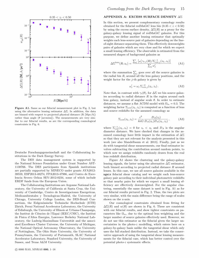
10−3
10−2
10−1
wgg(R
)
0.35 < zl < 0.50
100 101
R [Mpc/h]
10−1
100
101
∆Σ
(R)
[Mh/p
c2]
Figure A1. Same as our fiducial measurement plot in Fig. 2, butusing the alternative lensing estimator ∆Σ. In addition, the data
are binned with respect to projected physical distance (R [Mpc/h])rather than angle (θ [arcmins]). The measurements are very sim-
ilar to our fiducial results, as are the corresponding cosmological
constraints in Fig. 6.
Deutsche Forschungsgemeinschaft and the Collaborating In-stitutions in the Dark Energy Survey.
The DES data management system is supported bythe National Science Foundation under Grant Number AST-1138766. The DES participants from Spanish institutionsare partially supported by MINECO under grants AYA2012-39559, ESP2013-48274, FPA2013-47986, and Centro de Exce-lencia Severo Ochoa SEV-2012-0234, some of which includeERDF funds from the European Union.
The Collaborating Institutions are Argonne National Lab-oratory, the University of California at Santa Cruz, the Uni-versity of Cambridge, Centro de Investigaciones Energeticas,Medioambientales y Tecnologicas-Madrid, the University ofChicago, University College London, the DES-Brazil Con-sortium, the Eidgenossische Technische Hochschule (ETH)Zurich, Fermi National Accelerator Laboratory, the Universityof Edinburgh, the University of Illinois at Urbana-Champaign,the Institut de Ciencies de l’Espai (IEEC/CSIC), the Institutde Fısica d’Altes Energies, Lawrence Berkeley National Lab-oratory, the Ludwig-Maximilians Universitat and the associ-ated Excellence Cluster Universe, the University of Michigan,the National Optical Astronomy Observatory, the Universityof Nottingham, The Ohio State University, the University ofPennsylvania, the University of Portsmouth, SLAC NationalAccelerator Laboratory, Stanford University, the University ofSussex, and Texas A&M University.
APPENDIX A: EXCESS SURFACE DENSITY ∆Σ
In this section, we present complementary cosmology resultsobtained for the fiducial redMaGiC lens bin (0.35 < z < 0.50)by using the excess surface density, ∆Σ(R) as a proxy for thegalaxy-galaxy lensing signal of redMaGiC galaxies. For thispurpose, we define another lensing estimator that optimallyweights each lens-source pair of galaxies depending on the line-of-sight distance separating them. This effectively downweightspairs of galaxies which are very close and for which we expecta small lensing efficiency. The observable is estimated from themeasured shapes of background galaxies as
∆Σlens(R; zL) =
∑j
[ω′jγt,j(R)/Σ−1
crit,j(zL, zs)]∑
j ω′j
(A1)
where the summation∑j goes over all the source galaxies in
the radial bin R, around all the lens galaxy positions, and theweight factor for the j-th galaxy is given by
ω′j = ωj Σ−2crit,j(zL, zs) . (A2)
Note that, in contrast with γt(θ), for ∆Σ we bin source galax-ies according to radial distance R in the region around eachlens galaxy, instead of angular scale θ. In order to estimatedistances, we assume a flat ΛCDM model with Ωm = 0.3. Theweighting factor Σcrit(zL, zs) is computed as a function of lensand source redshifts for the assumed cosmology as
Σcrit(zL, zs) =c2
4πG
DA(zs)
DA(zL)DA(zL, zs), (A3)
where Σ−1crit(zL, zs) = 0 for zs < zL and DA is the angular
diameter distance. We have checked that changes in the as-sumed cosmology have little impact in the estimation of ∆Σso that they are not relevant for the analysis presented in thiswork (see also Mandelbaum et al. 2013). Finally, just as wedo with tangential shear measurements, our final estimator in-volves subtracting the contribution around random points, towhich now we assign redshifts randomly drawn from the reallens redshift distribution.
Figure A1 shows the clustering and the galaxy-galaxylensing signals, the latter using the alternative ∆Σ estimator,both binned according to projected radial distance R aroundlenses. In this case, we use all source galaxies available in thengmix fiducial shear catalog and we weight each lens-sourcegalaxy pair according to their individual photometric redshiftsso that nearby pairs for which we expect a small lensing ef-ficiency are effectively downweighted. For the angular clus-tering, essentially the same dataset is used in Fig. A1 as forour fiducial results pictured in Fig. 2. Thus, the two plots arevery similar, with the main difference being the range of scalesshown on the x-axis.
Our cosmological constraints obtained from fitting for∆Σ(R) and w(R) are shown in Fig. 6. These are consistentwith our fiducial results, and show tighter constraints on pa-rameters like Ωm, due to the optimal lens weighting and thelarger number of source galaxies effectively used. However, wedo not use this estimator as the fiducial given the larger un-certainties in the photo-z modelling, which enters here on agalaxy-by-galaxy basis unlike the tangential shear which onlyuses the full stacked distribution. Instead, we take the conser-vative approach of using the tangential shear lensing measure-ments for the fiducial case, which has better control over thepotential photo-z systematic effects.
c© 0000 RAS, MNRAS 000, 1–18
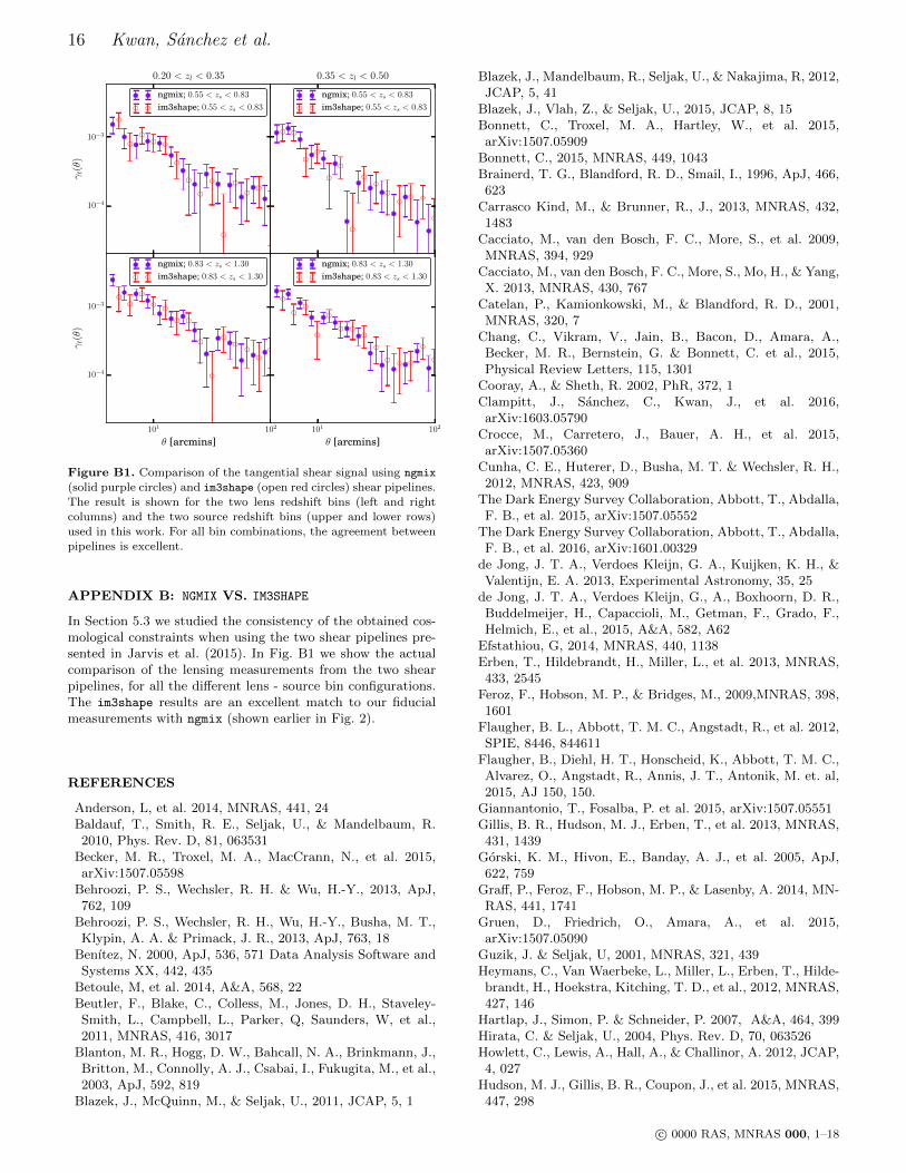
16 Kwan, Sanchez et al.
θ [arcmins]
10−4
10−3
γt(θ)
0.20 < zl < 0.35
ngmix; 0.55 < zs < 0.83
im3shape; 0.55 < zs < 0.83
0.35 < zl < 0.50
ngmix; 0.55 < zs < 0.83
im3shape; 0.55 < zs < 0.83
101 102
θ [arcmins]
10−4
10−3
γt(θ)
ngmix; 0.83 < zs < 1.30
im3shape; 0.83 < zs < 1.30
101 102
θ [arcmins]
ngmix; 0.83 < zs < 1.30
im3shape; 0.83 < zs < 1.30
Figure B1. Comparison of the tangential shear signal using ngmix
(solid purple circles) and im3shape (open red circles) shear pipelines.
The result is shown for the two lens redshift bins (left and right
columns) and the two source redshift bins (upper and lower rows)used in this work. For all bin combinations, the agreement between
pipelines is excellent.
APPENDIX B: NGMIX VS. IM3SHAPE
In Section 5.3 we studied the consistency of the obtained cos-mological constraints when using the two shear pipelines pre-sented in Jarvis et al. (2015). In Fig. B1 we show the actualcomparison of the lensing measurements from the two shearpipelines, for all the different lens - source bin configurations.The im3shape results are an excellent match to our fiducialmeasurements with ngmix (shown earlier in Fig. 2).
REFERENCES
Anderson, L, et al. 2014, MNRAS, 441, 24Baldauf, T., Smith, R. E., Seljak, U., & Mandelbaum, R.2010, Phys. Rev. D, 81, 063531
Becker, M. R., Troxel, M. A., MacCrann, N., et al. 2015,arXiv:1507.05598
Behroozi, P. S., Wechsler, R. H. & Wu, H.-Y., 2013, ApJ,762, 109
Behroozi, P. S., Wechsler, R. H., Wu, H.-Y., Busha, M. T.,Klypin, A. A. & Primack, J. R., 2013, ApJ, 763, 18
Benıtez, N. 2000, ApJ, 536, 571 Data Analysis Software andSystems XX, 442, 435
Betoule, M, et al. 2014, A&A, 568, 22Beutler, F., Blake, C., Colless, M., Jones, D. H., Staveley-Smith, L., Campbell, L., Parker, Q, Saunders, W, et al.,2011, MNRAS, 416, 3017
Blanton, M. R., Hogg, D. W., Bahcall, N. A., Brinkmann, J.,Britton, M., Connolly, A. J., Csabai, I., Fukugita, M., et al.,2003, ApJ, 592, 819
Blazek, J., McQuinn, M., & Seljak, U., 2011, JCAP, 5, 1
Blazek, J., Mandelbaum, R., Seljak, U., & Nakajima, R, 2012,JCAP, 5, 41
Blazek, J., Vlah, Z., & Seljak, U., 2015, JCAP, 8, 15Bonnett, C., Troxel, M. A., Hartley, W., et al. 2015,arXiv:1507.05909
Bonnett, C., 2015, MNRAS, 449, 1043Brainerd, T. G., Blandford, R. D., Smail, I., 1996, ApJ, 466,623
Carrasco Kind, M., & Brunner, R., J., 2013, MNRAS, 432,1483
Cacciato, M., van den Bosch, F. C., More, S., et al. 2009,MNRAS, 394, 929
Cacciato, M., van den Bosch, F. C., More, S., Mo, H., & Yang,X. 2013, MNRAS, 430, 767
Catelan, P., Kamionkowski, M., & Blandford, R. D., 2001,MNRAS, 320, 7
Chang, C., Vikram, V., Jain, B., Bacon, D., Amara, A.,Becker, M. R., Bernstein, G. & Bonnett, C. et al., 2015,Physical Review Letters, 115, 1301
Cooray, A., & Sheth, R. 2002, PhR, 372, 1Clampitt, J., Sanchez, C., Kwan, J., et al. 2016,arXiv:1603.05790
Crocce, M., Carretero, J., Bauer, A. H., et al. 2015,arXiv:1507.05360
Cunha, C. E., Huterer, D., Busha, M. T. & Wechsler, R. H.,2012, MNRAS, 423, 909
The Dark Energy Survey Collaboration, Abbott, T., Abdalla,F. B., et al. 2015, arXiv:1507.05552
The Dark Energy Survey Collaboration, Abbott, T., Abdalla,F. B., et al. 2016, arXiv:1601.00329
de Jong, J. T. A., Verdoes Kleijn, G. A., Kuijken, K. H., &Valentijn, E. A. 2013, Experimental Astronomy, 35, 25
de Jong, J. T. A., Verdoes Kleijn, G., A., Boxhoorn, D. R.,Buddelmeijer, H., Capaccioli, M., Getman, F., Grado, F.,Helmich, E., et al., 2015, A&A, 582, A62
Efstathiou, G, 2014, MNRAS, 440, 1138Erben, T., Hildebrandt, H., Miller, L., et al. 2013, MNRAS,433, 2545
Feroz, F., Hobson, M. P., & Bridges, M., 2009,MNRAS, 398,1601
Flaugher, B. L., Abbott, T. M. C., Angstadt, R., et al. 2012,SPIE, 8446, 844611
Flaugher, B., Diehl, H. T., Honscheid, K., Abbott, T. M. C.,Alvarez, O., Angstadt, R., Annis, J. T., Antonik, M. et. al,2015, AJ 150, 150.
Giannantonio, T., Fosalba, P. et al. 2015, arXiv:1507.05551Gillis, B. R., Hudson, M. J., Erben, T., et al. 2013, MNRAS,431, 1439
Gorski, K. M., Hivon, E., Banday, A. J., et al. 2005, ApJ,622, 759
Graff, P., Feroz, F., Hobson, M. P., & Lasenby, A. 2014, MN-RAS, 441, 1741
Gruen, D., Friedrich, O., Amara, A., et al. 2015,arXiv:1507.05090
Guzik, J. & Seljak, U, 2001, MNRAS, 321, 439Heymans, C., Van Waerbeke, L., Miller, L., Erben, T., Hilde-brandt, H., Hoekstra, Kitching, T. D., et al., 2012, MNRAS,427, 146
Hartlap, J., Simon, P. & Schneider, P. 2007, A&A, 464, 399Hirata, C. & Seljak, U., 2004, Phys. Rev. D, 70, 063526Howlett, C., Lewis, A., Hall, A., & Challinor, A. 2012, JCAP,4, 027
Hudson, M. J., Gillis, B. R., Coupon, J., et al. 2015, MNRAS,447, 298
c© 0000 RAS, MNRAS 000, 1–18
Cosmology from the Dark Energy Survey 17
Jarvis, R. M., Bernstein, G.,& Jain, B., 2004, MNRAS, 352338
Jarvis, M., Sheldon, E., Zuntz, J., et al. 2015,arXiv:1507.05603
Joachimi, B., Mandelbaum, R., Abdalla, F. B. & Bridle, S. L.,2011, A&A, 527, 26
Joachimi, B., Cacciato, M., Kitching, T. D., Leonard, A.,Mandelbaum, R., Schafer, B. M., Sifon, C. Hoekstra, H.,et al., Space Science Reviews, 193, 1
Kaiser, N., 1992, ApJ, 388, 272,Kuijken, K., Heymans, C., Hildebrandt, H., et al. 2015, MN-RAS, 454, 3500
Landy, S. D., & Szalay, A. S. 1993, ApJ, 412, 64Lawrence, E., Heitmann, K., White, M., Higdon, D., Wagner,C., Habib, S., & Williams, B., 2010, ApJ, 713, 1322
Leauthaud, A., Tinker, J., Bundy, K., et al. 2012, ApJ, 744,159
Lehmann, B. V., Mao, Y.-Y., Becker, M. R., Skillman, S. W.& Wechsler, R. H. 2015, arXiv:1510.05651
Leistedt, B., Peiris, H. V., Elsner, F., et al. 2015,arXiv:1507.05647
Lewis, A., Challinor, A., & Lasenby, A. 2000, ApJ, 538, 473Li, T. S., DePoy, D. L., Marshall, J. L., et al. 2016,arXiv:1601.00117
Limber, D., N., 1953, ApJ, 117, 134Mandelbaum, R., Seljak, U., Cool, R. J., et al. 2006, MNRAS,372, 758
Mandelbaum, R., Seljak, U., & Hirata, C. M. 2008, JCAP, 8,6
Mandelbaum, R., Slosar, A., Baldauf, T., et al. 2013, MN-RAS, 432, 1544
Mao, Y-Y, Williamson, M., & Wechsler, R. H., 2015, ApJ,810, 21
Marian, L, Smith, R. E. & Angulo, R. E., 2015, MNRAS, 451,1418
McDonald, P., 2006, Phys. Rev. D, 74, 103512Miyazaki, S., Komiyama, Y., Nakaya, H., Kamata, Y., Doi,Y., Hamana, T., Karoji, H., Furusawa, H., et al., 2012,SPIE, 8446, 0Z
Monet, D. G., Levine, S. E., Canzian, B., Ables, H. D., et al.2003, AJ, 125, 984
More, S., Miyatake, H., Mandelbaum, R., et al. 2015, ApJ,806, 2
Norberg, P., Baugh, C. M., Gaztanaga, E., & Croton, D. J.2009, MNRAS, 396, 19
Park, Y., Krause, E., Dodelson, S., et al. 2015,arXiv:1507.05353
The Planck Collaboration, Ade., P. A. R et al, 2015,arXiv:1502.01589
Reddick, R. M., Wechsler, R. H., Tinker, J. L., & Behroozi,P. S., 2013, ApJ, 771, 30
Ross, A., J. et al. 2011, MNRAS, 417, 1350Ross, A. J. et al. 2012, MNRAS, 424, 564Ross, A. J. et al. 2014, MNRAS, 437, 1109Ross, A. J. et al. 2015, MNRAS, 449, 835Rozo, E., Rykoff, E. S., Becker, M., Reddick, R. M., & Wech-sler, R. H. 2015, MNRAS, 453, 38
Rozo, E., Rykoff, E. S., Abate, A., et al. 2015,arXiv:1507.05460
Rykoff, E. S., Rozo, E., Busha, M. T., et al. 2014, ApJ, 785,104
Sadeh I., Abdalla F., B., Lahav O., 2015, arXiv:1507.00490Seljak U., 2000, MNRAS, 318, 203Sanchez, C., Carrasco Kind, M., Lin, H., et al. 2014, MNRAS,
445, 1482Sheldon, E. S., Johnston, D. E., Frieman, J. A., et al. 2004,AJ, 127, 2544
Sheldon, E. S. 2014, MNRAS, 444, L25Sifon, C., Cacciato, M., Hoekstra, H., et al. 2015, MNRAS,454, 3938
Singh, S., & Mandelbaum, R., 2015, MNRAS, 450, 2195Smith, R. E., Peacock, J. A., Jenkins, A., et al. 2003, MN-RAS, 341, 1311
Springel, V., 2005, MNRAS, 364, 1105Suchyta, E., Huff, E. M., Aleksic, J., Melchior, P., et al. 2016,MNRAS, 457, 786
Takahashi, R., Sato, M., Nishimichi, T., Taruya, A., & Oguri,M. 2012, ApJ, 761, 152
Troxel, M. A. & Ishak, M., 2015, PhR, 558, 1TTyson, J. A., Valdes, F., J. F., & Mills, A. P., Jr. 1984, ApJL,281, L59
van Uitert, E., Cacciato, M., Hoekstra, H., et al. 2016,arXiv:1601.06791
Velander, M., van Uitert, E., Hoekstra, H., et al. 2014, MN-RAS, 437, 2111
Vikram, V., Chang, C., Jain, B., et al. 2015, Phys. Rev. D,92, 022006
Viola, M., Cacciato, M., Brouwer, M., et al. 2015, MNRAS,452, 3529
Yang, X., Mo, H. J., van den Bosch, F. C., et al. 2006, MN-RAS, 373, 1159
Yoo, J., & Seljak, U. 2012, Phys. Rev. D, 86, 083504York, D. G., Adelman, J., Anderson, J. E., Jr., Ander-son, S. F., Annis, J., Bahcall, N. A., Bakken, J. A., Bark-houser, R., et al., 2000, AJ, 120, 9
Zuntz, J., Kacprzak, T., Voigt, L., et al. 2013, MNRAS, 434,1604
Zuntz, J., Paterno, M., Jennings, E., et al. 2015, Astronomyand Computing, 12, 45
AFFILIATIONS
1 Department of Physics and Astronomy, University ofPennsylvania, Philadelphia, PA 19104, USA2 Institut de Fısica d’Altes Energies (IFAE), The BarcelonaInstitute of Science and Technology, Campus UAB, 08193Bellaterra (Barcelona) Spain3 Center for Cosmology and Astro-Particle Physics, The OhioState University, Columbus, OH 43210, USA4 Institut de Ciencies de l’Espai, IEEC-CSIC, Campus UAB,Carrer de Can Magrans, s/n, 08193 Bellaterra, Barcelona,Spain5 Jodrell Bank Center for Astrophysics, School of Physicsand Astronomy, University of Manchester, Oxford Road,Manchester, M13 9PL, UK6 Department of Physics, ETH Zurich, Wolfgang-Pauli-Strasse16, CH-8093 Zurich, Switzerland7 Department of Physics, Stanford University, 382 Via PuebloMall, Stanford, CA 94305, USA8 Kavli Institute for Particle Astrophysics & Cosmology, P.O. Box 2450, Stanford University, Stanford, CA 94305, USA9 Fermi National Accelerator Laboratory, P. O. Box 500,Batavia, IL 60510, USA10 Kavli Institute for Cosmological Physics, University ofChicago, Chicago, IL 60637, USA11 Department of Physics, University of Chicago, 5640 South
c© 0000 RAS, MNRAS 000, 1–18
18 Kwan, Sanchez et al.
Ellis Avenue, Chicago, IL, 60637, USA12 Jet Propulsion Laboratory, California Institute of Technol-ogy, 4800 Oak Grove Dr., Pasadena, CA 91109, USA13 Institute of Astronomy, University of Cambridge, Mading-ley Road, Cambridge CB3 0HA, UK14 Kavli Institute for Cosmology, University of Cambridge,Madingley Road, Cambridge CB3 0HA, UK15 SLAC National Accelerator Laboratory, Menlo Park, CA94025, USA16 Department of Physics, ETH Zurich, Wolfgang-Pauli-Strasse 16, CH-8093 Zurich, Switzerland17 Department of Physics & Astronomy, University CollegeLondon, Gower Street, London, WC1E 6BT, UK18 Institucio Catalana de Recerca i Estudis Avancats, E-08010Barcelona, Spain19 Department of Physics, University of Arizona, Tucson, AZ85721, USA20 Brookhaven National Laboratory, Bldg 510, Upton, NY11973, USA21 Cerro Tololo Inter-American Observatory, National OpticalAstronomy Observatory, Casilla 603, La Serena, Chile22 Department of Physics and Electronics, Rhodes University,PO Box 94, Grahamstown, 6140, South Africa23 CNRS, UMR 7095, Institut d’Astrophysique de Paris,F-75014, Paris, France24 Sorbonne Universites, UPMC Univ Paris 06, UMR 7095,Institut d’Astrophysique de Paris, F-75014, Paris, France25 Laboratorio Interinstitucional de e-Astronomia - LIneA,Rua Gal. Jose Cristino 77, Rio de Janeiro, RJ - 20921-400,Brazil26 Observatorio Nacional, Rua Gal. Jose Cristino 77, Rio deJaneiro, RJ - 20921-400, Brazil27 Department of Astronomy, University of Illinois, 1002 W.Green Street, Urbana, IL 61801, USA28 National Center for Supercomputing Applications, 1205West Clark St., Urbana, IL 61801, USA29 Institute of Cosmology & Gravitation, University ofPortsmouth, Portsmouth, PO1 3FX, UK30 School of Physics and Astronomy, University of Southamp-ton, Southampton, SO17 1BJ, UK31 Excellence Cluster Universe, Boltzmannstr. 2, 85748Garching, Germany32 Faculty of Physics, Ludwig-Maximilians-Universitat,Scheinerstr. 1, 81679 Munich, Germany33 Department of Astronomy, University of Michigan, AnnArbor, MI 48109, USA34 Department of Physics, University of Michigan, Ann Arbor,MI 48109, USA35 Department of Physics, The Ohio State University, Colum-bus, OH 43210, USA36 Australian Astronomical Observatory, North Ryde, NSW2113, Australia37 Departamento de Fısica Matematica, Instituto de Fısica,Universidade de Sao Paulo, CP 66318, CEP 05314-970, SaoPaulo, SP, Brazil38 George P. and Cynthia Woods Mitchell Institute forFundamental Physics and Astronomy, and Department ofPhysics and Astronomy, Texas A&M University, CollegeStation, TX 77843, USA39 Department of Astronomy, The Ohio State University,Columbus, OH 43210, USA40 Department of Astrophysical Sciences, Princeton Univer-sity, Peyton Hall, Princeton, NJ 08544, USA41 Max Planck Institute for Extraterrestrial Physics, Giessen-
bachstrasse, 85748 Garching, Germany 42 Department ofPhysics and Astronomy, Pevensey Building, University ofSussex, Brighton, BN1 9QH, UK43 Centro de Investigaciones Energeticas, Medioambientales yTecnologicas (CIEMAT), Madrid, Spain44 ICTP South American Institute for Fundamental ResearchInstituto de Fısica Teorica, Universidade Estadual Paulista,Sao Paulo, Brazil45 Argonne National Laboratory, 9700 South Cass Avenue,Lemont, IL 60439, USA
This paper has been typeset from a TEX/ LATEX file preparedby the author.
c© 0000 RAS, MNRAS 000, 1–18


![Customer Segmentation Using Clustering and Data Mining ...twiki.di.uniroma1.it/pub/BI/WebHome/ClusteringforMarketSegmentation.pdf · optimum results. [3]. Clustering is a type of](https://img.pdfslide.us/doc/110x75/5e39fc718eb51823ec77ad65/customer-segmentation-using-clustering-and-data-mining-twikidi-optimum-results.jpg)