Corrosion in Polythermal Loop Systems II. A Solid-State ...moltensalt.org/references/static/downloads/pdf/ORNL-4575.pdf'0 - p ornl4575, volume 2 contract no. w-7405-eng-26 metau and

' 0

- P

O R N L 4 5 7 5 , V o l u m e 2

C o n t r a c t N o . W-7405-eng-26

METAU AND CERAMICS D I V I S I O N

CORRCEION I N POLYTHERMAL LOOP SYSTEMS

WITH AND WITHOUT LIQUID FILM EFFECTS 11. A SOLID-STATE DIFFUSION MECHANISM

R. B. Evans I11 J. W. K o g e r J. H. D e V a n

This report was prepared as an account of work sponsored by the United States Government. Neither the United States nor the United States Atomic Energy Commission, nor any of their employees, nor any of their contractors, subcontractors, or their employees, makes any warranty. express or implied. or assumes any legal liability or responsibility for the accuracy, completeness or usefulness of any information, apparatus, product or process disclosed, or represents that its use would not infringe privately owned rights.

JUNE 1971

OAK RLDGE NATIONAL LA3ORATORY Oak R i d g e , Tennessee

operated by UNION CARBIDE CORPORATION

for the U. S. ATOMIC ENERGY COMMISSION

Q

B

Y

.

iii

CONTENTS

, .

c

. B

.

Abstract . . . . . . . . . . . . . . . . . . . . Nomenclature . . . . . . . . . . . . . . . . . . Introduction . . . . . . . . . . . . . . . . . . Fundamental Concepts . . . . . . . . . . . . . .

Basic Diffusion Relationships . . . . . . . Surface Behavior . . . . . . . . . . . . . .

Equilibrium Ratio . . . . . . . . . . . Reaction Rates . . . . . . . . . . . . . . Mass Transfer Across Liquid Films . . . Combined Reaction Rate-Film Resistances Surface Effects Referred t o the Alloy .

. . . . . . . . . 1

. . . . . . . . . 2

. . . . . . . . . 5

. . . . . . . . . 8 9

. . . . . . . . . 12

. . . . . . . . . 12

. . . . . . . . . u

. . . . . . . . . 16

. . . . . . . . . 17

. . . . . . . . . 18

. . . . . . . . .

Transient Solutions . . . . . . . . . . . . . . . . . . . . . . . 19 Review of the Equations . . . . . . . . . . . . . . . . . . . 19

Application t o Sodium-Inconel600 Systems . . . . . . . . . . 24

Reference and Prototype Loops . . . . . . . . . . . . . . . . 26 The Reference Loop . . . . . . . . . . . . . . . . . . . . 26 A Prototype Loop . . . . . . . . . . . . . . . . . . . . . 28

Quasi-Steady-State Solution . . . . . . . . . . . . . . . . . . . 32 Statement of the Problem and Objectives . . . . . . . . . . . 32 Solution i n Terms of the Prototype Loop . . . . . . . . . . . 36

Discussion of Sodium-Inconel600 Results . . . . . . . . . . . . . 46

Application t o Molten-Salt Systems . . . . . . . . . . . . . . . . Thermal Convection Loops . . . . . . . . . . . . . . . . . . . 50

Discussion . . . . . . . . . . . . . . . . . . . . . . . . . . 54 Transient Factors . . . . . . . . . . . . . . . . . . . . . . 55 Quasi-Steady-State Solutions . . . . . . . . . . . . . . . . . 59

Discussion of Molten-Salt Results . . . . . . . . . . . . . . . . 64

Temperature Profiles and Loop Configurations . . . . . . . . . . . 26

Predicted Results for Sodium-Inconel 600 Systems . . . . . . . 43

50

Redox Corrosion Equilibria and Systems Selected for

Summary . . . . . . . . . . . . . . . . . . . . . . . . . . . . . 69

,

L,

V

hd

I

Y I

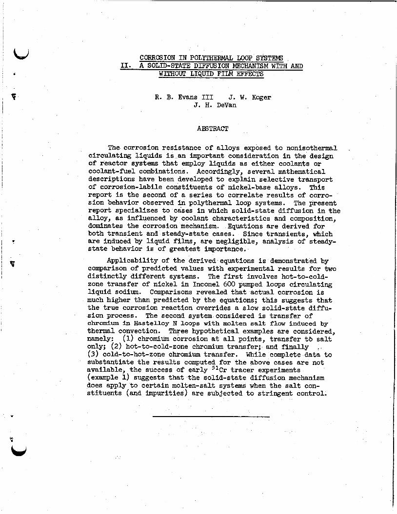
CORROSION I N POLYTHEFMAL LOOP SYSTEIB A SOLID-STATE DIFFUSION MECHANISM WITH AND

WITHOUT LIQUID FILM EFFECTS 11.

R. B. Evans I11 J. W. Koger J. H. DeVan

ABSTRACT

The corrosion resistance of alloys exposed t o nonisotherml circulating liquids i s an important consideration i n the design of reactor systems tha t employ liquids as either coolants or coolant-fuel combinations. Accordingly, several mathematical descriptions have been developed t o explain selective transport of corrosion-labile constituents of nickel-base alloys. This report i s the second of a series t o correlate results of corrosion behavior observed i n polythermal loop systems. The present report specializes t o cases i n which solid-state diffusion i n the alloy, as influenced by coolant characteristics and composition, dominates the corrosion mechanism. both transient and steady-state cases. are induced by liquid films, are negligible, analysis of steady- s t a t e behavior i s of greatest importance.

comparison of predicted values w i t h experimental resul ts for two dis t inc t ly different systems. zone transfer of nickel i n Inconel 600 pumped loops circulating l iquid sodium. much higher than predicted by the equations; th i s suggests tha t the t rue corrosion reaction overrides a slow solid-state diffusion process. chromium i n Hastelloy N loops with molten salt flow induced by thermal convection. namely: only; (2) hot-to-cold-zone chromium transfer; and f ina l ly (3) cold-to-hot-zone chromium transfer. substantiate the resul ts computed for the above cases a re not available, the success of early 51Cr t racer experiments (example 1) suggests that the solid-state diffusion mechanism does apply t o certain molten-salt systems when the salt con- s t i tuents (and impurities) are subjected t o stringent control.

Equations are derived for Since transients, which

Applicability of the derived equations i s demonstrated by

The first involves hot-to-cold-

Comparisons revealed that actual corrosion i s

The second system considered i s transfer of

(1) chromium corrosion a t a n points, transfer t b salt

While complete data t o

Three hypothetical examples are considered,

I

2

NOMENCLATURE

a = Subscript denoting alloy; superscript denoting act ivi ty .

M a = Activity of alloy constituent M, no units. % = Total l iquid exposed area of loop alloy, cm2.

= Cross-sectional area of loop tubing, cm2. AZ = Internal peripheral area of loop tubing, cm2.

b = Slope of a l inear T versus z segment, "K/cm. c = Subscript denoting cold zone.

i c = Constant group, 4 x a p a r t ~ , g cm-1 sec-1/2.

AXS

c = Integration constant with respect t o w, i = 1, 2, Wt. frac. sec.

C' = Constant group, (K /%IC, g cm-1 sec-1/2. P

d = Symbol for dissolved metallic species.

D = Diffusion coefficient of M(s) - i n a l l o y , cm2/sec. Do = Preexponential term, D/exp(-ED/RT), cm2/sec. Dm = Mutual diffusion coefficient of M(d) - i n l iquid metal, cm2/sec.

e = The transcendental number 2.7l828 ......., no units. 7 exp(z) = The exponential function of T, e , no units.

erf(v) = The error function of v, 6" e-T dT, no units. 2

erfc(v) = The complementary error function of v, 1 - erf(v), no units. 03

E1(u.) = First-order exponential function of u., ./ (e"/T)dT, no units. J .. J U j

LJ I

U.

Ei(u.) = The "i" exponential function of u IJ (e"/.t)dr, no units. J j '- ED = Activation energy fo r solid-state diffusion of M( - s) , cal/mole.

= Energy required t o dissolve M i n l iquid metal, cal/mole. Esoln f = Fraction of %; when Axs i s constant, f = z/L.

f ( p ) = Location of balance point where jM = 0 and k = %. P

03 - -st'dtf . f (w , s ) = Laplace transform of F(w,t),

F(w,t) = An arbi t rary function of w and t.

F(w,t)e

g = Symbol denoting gram mass. - g = Symbol denoting gas.

G = Gibb' s potential or f ree energy, cal/mole. h = Film coefficient for mass transfer, cm/sec. h = Combined solution r a t e - film coefficient, cm/sec.

c

ir

-

3

e

I I

h' = Subscript denoting hot zone.

H = m e product %(h/D)(Pj/Pa>(ma/%), cm'l.

i = Index 1 at f = 0 fo r function below.

AH = Enthalpy difference, cal/mole.

I. .(a/E) = An integrated function along extended z coordinate from 1J

Ei t o tj,rcm. j = Index p or 2 a t balance point or f = 1 f o r function above.

jM = ~ s s f lux of species M, g cm-2 sec-1/2.

JM = Atomic or molecular f lux of species M, mole

kl = Solution rate constant, cm/sec. .

k2 = Deposition rate constant, cm/sec.

I?' = Equilibrium constant, k, a a /k2 , no units.

seco1i2. k = Boltzmann constant = 1.38 X

kla = Solution r a t e constant, mole

k2& = Deposition r a t e constant, mole

g cm2 sec'l O r 1 ,

sec'l.

sec'l.

Ky = Activity coefficient r a t i o > YM(d)/YM(g)> units depend On - choice of standard states for %.

K, = Preexponential factor %/exp(-Esoln/RT), no units.

K = Balance point value of 5, no units. 5 = Ekperimental solubi l i ty constant, no units. P

1 = Subscript denoting liquid. L = Total loop length, cm. m = Molecular or atomic weight, @;/mole.

M = Symbol denoting m e t a l constituent subject t o corrosion. AM(t) = Mass or weight of M transferred, Q .

NRe = Reynolds number, 2r'Vzp/p. Nsc = Schmidt number, p/pDm, no units. Nsh = Sherwood number for mass transfer, 2hrf DMe, no units.

p = Symbol or subscript denoting balance point. q = A transformation variable, (s/D),l2, cm. Q = Volumetric f l a w rate i n loop, cm3/sec. r = Radial distance measured from the center of the loop tubing, cm.

M r = Atomic radius of M(d) i n l iquid metal, cm. r' = Inside radius of loop tubing, cm.

-

4

R = Gas constant used i n exponential terms, 1.987 c a l mole-’ Or’.

s = Laplace transformation variable, sec‘l.

s = Symbol denoting solid solution.

t = Time, sec. T = Temperature, OF, O C , or OK.

AT = Temperature drap along a segment of z, Ol?, O C , or OK.

u = Dimensionless variable, a/! no units. j 3’ v = The argument w / ( 4 ~ t ) 1 / 2 , no units. Vz = Liquid flow velocity, &/Axs, cm/sec.

w = Distance of l inear diffusion, normal t o AZ, of M(g) in

x = Concentration of M ( s ) - i n alloy expressed as weight fraction, alloy, cm.

no units. x = Concentration of M ( s ) - i n as-received alloy. 3 = Surface concentration of M ( s ) as a function of T along z. a

x ( w , t ) = Concentration of M ( s ) - i n diffusion region as a function of position and time.

x* = Alloy concentration of M(g) equivalent t o l iquid concentration

& = Alloy concentration of M ( s ) - equivalent t o equilibrium liquid

of M(d) - a t the l iquid side of the l iquid film.

concentration a t liquid-solid interface. - x = Concentration of M ( s ) - i n alloy expressed as atomic fraction,

no units. AX = The concentration difference, yn, (O,t) - xa, no units.

Lm* = The concentration difference, fi - xa, no units. y = Concentration of M(d) - i n bulk l iquid expressed as weight

fraction; it corresponds t o y* when transients are discussed, no units.

fl= Concentration of M(d) - a t metal-film interface, no units.

Y = Equilibrium or saturation concentration of M(d) - i n a unit

ac t iv i ty container. - = Concentration of M(d) - i n bulk l iquid expressed as weight

fraction, no units.

.

V

c

w

.-

- I

5

W . c ¶

z = Linear f l a w coordinate for v or Q, cm. a! = The factor (ED)/(2bR), cm.

)/2bR > 1, cm. 2Esoln a!’ = The factor ( E ~ - a!’f = The factor a!’ < 1, cm.

B(uj) = The factor u exp(u.)El(u ), no units. j J j

7 = Activity coefficients, units selected t o make aM dimensionless.

A = Sylnbol t o denote difference. E = Extended z coordinate = a!/uj, cm. p = Viscosity coefficient of the l iquid metal, g cm-l sec’l. I[ = The transcendental number 3.l416..., no units. p = Mass or weight density, g/cm3. T = Dummy variable of integration, no units.

= Concentration difference for hot zone, ynf (0,t) - % (w, t ) , @hr no units.

* @E’ = Concentration difference for hot zone when liquid fi lm i s

t present, - yn, (w, t ) , no units.

presence of l iquid film, xe(w,t) - xa, no units.

4 = 4; concentration difference for cold zone with and without C

INTRODUCTION

In a previous report1 (hereafter referred t o as Report I) atten-

t ion was given t o interpretations of corrosion behavior i n systems composed of liquid sodium c

Specific interest focused on experimental pumped loops that gave def ini te evidence that nickel and chromium moved from hot t o cold regions of the loops. about the solubi l i ty of chromium i n l iquid sodium; furthermore, the major component undergoing corrosion and transfer was nickel. Solubili ty

ained i n the nickel-base al loy Inconel 600.

Only nickel transfer was considered, because l i t t l e was known

w information i s of major importance because the manner i n which solubi l i ty

*

CM’ lR. B. Evans I11 and Paul Nelson, Jr., Corrosion i n Polythermal

Systems, I. Mass Transfer Limited by Surface and Interface Resistances as Compared with Sodium-Inconel Behavior, -4575, Vol. 1 (March 197’1).

6

increases with temperature governs the steady-state driving force for mass transfer around the loop.

The major effor t i n Report I was t o develop a simple system of equations that might describe the mass transfer as observed experimentally. The approach i n Report I was t o assme tha t the mass-transfer equations would f a l l in to the same patterns as those that describe heat transfer from hot t o cold zones under conditions of known external-temperature profiles and rates of f luid f l o w around the loop. For heat flow, the only resistances involved would be an overall coefficient that would com- pr i se the thermal conductivity of the walls and a heat-transfer film.

An analogous situation was assumed for mass transfer with the exception that the thermal conductivity term was replaced by a reaction-rate constant tha t was presumed t o be associated with a first-order dissolution react ion.

Predictions of corrosion based on the heat-transfer analog showed

tha t transient mass transfer effects decayed af te r negligibly short times (fractions of an hour). Steady-state corrosion rates calculated from the film coefficient alone were much greater than measured values. It w a s necessary t o invoke the reaction-fate constant t o increase the resistances and lower the computed resul ts i n order t o match experimen- t a l results. While t h i s "matching" could be done for resul ts of individual experiments, a consistent set of reaction constants for a l l results tha t would lead t o a general correlation could not be obtained. One of the prime reasons for the fa i lure of the mechanisms covered i n Report I

i s tha t the loop walls were not pure nickel. Rather, the walls were of

id .

Y

an alloy wherein solid-state diffusion effects influenced the overall behavior. These effects were ignored i n the equations of Report I.

The present report i s devoted t o another mathematical treatment of an idealized mass-transfer process wherein corrosion rates depend direct ly on the rate a t which consituents of alloys diffuse in to or out of container walls, as influenced by the condition of wall surfaces exposed t o a high-temperature liquid. Specifically, consideration i s

given t o cases for which solid-state diffusion controls mass transfer at a l l points i n a polythermal loop system containing circulating liquids.

.-

The container constituents of interest a re nickel-base alloys.

7

I -

.*

i

We have also considered the contributions of liquid-film resistances

acting simultaneously with the solid-state mechanism t o ascertain whether or not a suitable combined mechanism (our ultimate goal) could be attained. Unfortunately, t h i s approach was unsuccessful.

Three rather important assumptions are made i n our present derivations. First , effects of changes i n w a l l dimensions can be neglected. Second, the r a t e of diffusion i s unaffected by composition changes i n the diffusion zone of the alloy; i n other words, the diffusion coef-

f ic ien t i s not a function of concentration. l iquid i s pre-equilibrated with respect t o the amount of dissolved components so tha t the concentrations i n the l iquid do not vary appreciably w i t h position or time. both the "transient" and "quasi-steady-state" conditions tha t a re covered i n th i s report.

re la t ive t o reactor applications, .the basic approach i n assessing corrosion properties remains the same. One employs either thermal convection loops or pumped systems t o collect the data required. t h i s writing, sodium systems, which are of interest t o the Liquid Metal Fast Breeder R e a ~ t o r , ~ , ~ are under intensive study. treatment similar t o that t o be covered here was i n i t i a l l y roughed out i n 1957 under the auspices of the Aircraft Nuclear Propulsion (ANP) Project.4 The liquids of interest in th i s early effor t were molten fluoride salts. *

Third, the circulating

This l a t t e r boundary condition is embodied i n

It should be mentioned that, although many liquids have been studied

A t the time of

We should note a

The objective of the work leadi'ng t o the present report kas been t o carry out refinements of the early ANP treatments,4 and t o generalize the results t o permit t he i r application t o many systems tha t might

2Argonne National Laboratory, Liquid Metal Fast Breeder Reactor (LMFBR) Program Plan. Volume 1. Overall Plan, WASH-1101 (August 1968).

3Alkali Metal Coolants (Proceedings of a Symposium, Vienna, 28 November - 2 December, 19661, International Atomic Energy Agency, Vienna, 1967.

4R. B. Evans 111, ANP Program Quart. Progr. Rept. Dec. 31, 1957, oRNL2440, pp. 104-1l3.

i

5R. C. miant and A. M. Weinberg, "Molten Fluorides as Power Fuels," Nucl. Sci. Ehg. 22, 797-803 (1957). -

8

operate within the solid-state mechanism under consideration.

term and immediate objective i s t o determine whether a mechanism of t h i s type applies t o the migration of nickel i n the sodium-Inconel system i n high-velocity pumped loops.

A short-

One of the central conclusions of the present study i s tha t the solid-state mechanism clearly does not explain the observed corrosion behavior of the sodium-Inconel 600 system.

ever, the analytical work that was done is immediately and direct ly applicable t o Hastelloy N-molten salt thermal convection loops, i n which t h i s solid-state mechanism clearly does operate. Thus, the present work includes two separate topics: metals, another covering corrosion induced by constituents i n molten- salt systems.

On the posit ive side, haw-

one covering corrosion induced by l iquid

For ease of presentation, a rather unorthodox outline has been adapted for th i s report. variables, and the type of transients one might encounter. t o a discussion of l iquid mass-transfer films and the i r effects on the corrosion rates. t i ve corrosion a t quasi-steady-state (i. e., when the transient effect associated with liquid film resistance has diminished). appears because the predicted corrosion varies with the square root of

t h e . However, t o emphasize the meaning of the analytical results, detailed "example calculations" are given. liquid-metal application and three molten-salt applications. section i s a summary of the more important features of the equations and the i r applications.

F i r s t , we discuss basic diffusion relationships, Then we turn

Next, we derive and present equations fo r the cumula-

The term "quasi"

These make up the most irrrportant aspect of the report.

Separate discussions are presented for the The f ina l

FUNDAMENTAL CONCEPTS

It would be most convenient, f'rom the authors' standpoint, t o . proceed directly t o the task of sett ing up the diffusion relationships tha t take liquid phase mass transfer into account, show th i s t o be of l i t t l e importance, and proceed direct ly t o the quasi-steady-state solu- t ion based on the diffusion relationships. This i s the conventional

t

9

!

i 1

!

i

i j

I

i I

i I

j

I

i i I i

~

~ I I

hi .

c Y

method of presentation, but one immediately encounters fractional-

approach variables introduced by the nature of the alloys and chemistry of the liquids. Accordingly, we shall jump ahead of the film par t o f - the problem and start by writing dam some of the well-known expressions for solid-state diffusion i n order t o introduce the i.deas behind fractional-approach variables and t o enable recognition of integrated forms that emerge when f i l m resistances a re encountered.

Basic Diffusion Relationships

The basic relationships required are the concentration-profile equations that express the weight or mass fraction x(w,t) of an alloy constituent as a function of position across the w a l l , w, and time, t. We l e t w = r - r', where rf is the inner radius of the loop tubing.

The relationships derive from Fick's second l a w of diffusion, sometimes

called the Fourier equation, and apply t o both hot and cold zones of the system. These relationships are developed elsewhere.6J7 It i s suf- f ic ien t here t o point out just a few important features of the equations involving x(w,t). Only l inear diffusion along a single coordinate,g w, sha l l be considered.

The direction of w is normal t o the l iquid exposed surface, Az, where w = 0.

First , x(0,t) is assumed t o be constant with time.'

The container walls are inf in i te ly thick relat ive t o the effec- t i v e depth of the profile; thus x(w,t) = x the constituent, fo r a l l times.

the bulk concentration of a'

6R. V. Churchill, Modern Operational Mathematics i n Engineering, 1st ed., pp. 109-Il2, McGraw-Hill, New York, 1950.

7H. S. C a r s l a w and J. C. Jaeger, Conduction of Heat i n Solids, 2nd ed., pp. 5841, Oxford University Press, New York, 1959.

'The just i f icat ion for t h i s assumption w i l l become evident as we discuss the relationship between the concentration of an element a t the metal surface and i ts concentration i n the corrosion medium.

'The reader should not infer that use of w = r - rf means that a radial flow system i s t o be employed; we use w as a l inear flow coordinate, even though the container i s a cylindrical tube, because most of the alphabet has been reserved for other notation.

10

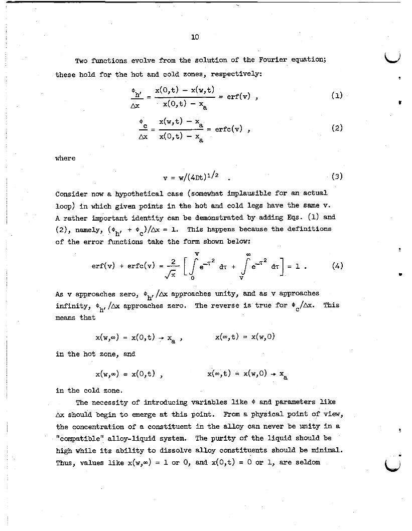
Two f'unctions

these hold for the

evolve from the solution of the Fourier equation;

hot and cold zones, respectively:

- - @h' - x(O,t) - x(w,t> = erf(v) ,

Ax x(O,t) - Xa

QC x(w,t) - Xa

ax x(0,t) - xa = erfc(v) , - =

where

Consider now a hypothetical case (somewhat implausible fo r an actual

loop) i n which given points i n the hot and cold legs have the same v. A rather important identity can be demonstrated by adding Eqs. (1) and (2), namely, (@ + @,)/Ax = 1.

of the error flmctions take the form shown below: This happens because the definitions h'

V m

erf(v) + erfc(v) = - 2 [ f eCr2 dr + Je-r2 dr] = 1 . (4 1 f i o V

As v approaches zero, Qhf /Ax approaches unity, and as v approaches infinity, Oh' /Ax approaches zero. means that

The reverse is t rue for @ /Ax. This C

x(wp) = x(0,t) + xa , x(+) = x(w,o)

i n the hot zone, and

x(w,4 = x(O,t) , x(+) = x(w,o) + xa

i n the cold zone. The necessity of introducing variables l i ke 4 and parameters l ike

Ax should begin t o emerge at th i s point. the concentration of a constituent i n the alloy can never be unity i n a

From a physical point of view,

"compatible" alloy-liquid system. high while i t s ab i l i t y t o dissolve alloy constituents should be minimal. Thus, values l ike x(w,m) = 1 or 0, and x(0,t) = 0 or 1, are seldom

The purity of the l iquid should be ?

I

. P

c 3

encountered i n practice. solution m u s t vanish at a l l boundaries except one.

language of partial dif'ferential equations, the heat equation must be

Yet, from a mathematical point of view, the Stated i n the

homogeneous; the same i s t rue for a l l but one of the boundary condi- tionslO,ll unless an additional equation i s involved. conditions usually concern an i n i t i a l or particular surface condition. For these reasons, f'ractional-approach variables are employed.

The nonhomogeneous

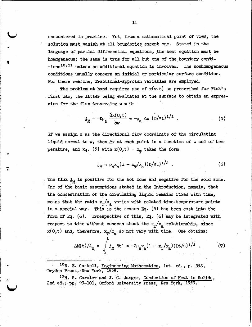
The problem a t hand requires use of x(w,t) as prescribed fo r Fick's first law, the l a t t e r being evaluated a t the surface t o obtain an expression fo r the flux traversing w = 0:

If we assign z as the directional f l aw coordinate o f t h e circulating l iqu id normal t o w, then Ax at each point is a function of z and of temperature, and Eq. (5) w i t h x(0,t) = % takes the form

The f lux j, is posit ive for the hot zone and negative for the cold zone. One of the basic assumptions stated i n the Introduction, namely, t ha t the concentration of the circulating l iquid remains fixed with t h e , means that the r a t i o ?/xa varies w i t h related time-temperature points i n a special way. This i s the reason Eq. ( 5 ) has been cast in to the

form of Eq. (6). Irrespective of this, Eq. (6) may be integrated with

respect t o time without concern about the %/xa relationship, since x(0,t) and, therefore, %/xa do not vary w i t h time. One obtains:

AM(t)/A Z = f jM dt' = -2paxa( 1 - %/xa) (Dt/n)1/2 . (7 0

'OR. E. Gaskell, Engineering Mathematics, 1st. ed., p. 358, Dryden Press, New York, 1958.

'1H. S . Carslaw and J. C. Jaeger, Conduction of Heat i n Solids, 2nd ed:,.pp. 99-101, Oxford University Press, New York, 1959.

Under the usual sign convention, a positive value of AM/A means tha t the metal constituent diffuses into the al loy (cold zone); negative values mean outward diff'usion (hot zone). We sha l l reverse t h i s Conven- tion, since we desire a balance of M with respect t o the liquid. solution behavior of most acceptable systems i s such tha t the l iquid

gains material i n the hot zone and loses material i n the cold zone. other words, xa > % i n the hot zone; xa < 5 i n the cold zone; notice tha t Eqs. (6) and (7) follow the adopted convention automatically. next mathematical operation involves integration along z, but t h i s requires some knuwledge of the manner inwhich z varies with T and, of

greater importance, the manner i n which T varies with x(0,t). t e r i s a problem i n chemistry t o which we nuw turn.

The

In

The

The lat-

Surface Behavior

Equilibrium Ratio

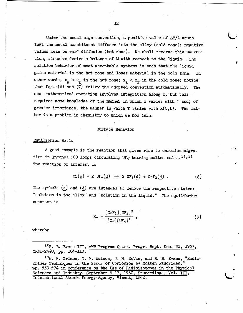
A good example i s the reaction tha t gives rise t o chromium migra- t ion i n Inconel 600 loops circulating UF4-bearing molten salts. 12,13

The reaction of in te res t i s

C r ( s ) - + 2 UFq(d) - =s 2 UF,(d) + CrFz(d) - . The symbols (E) and (d) - are intended t o denote the respective states: "solution i n the alloy" and "solution i n the liquid." constant i s

The equilibrium

whereby

12R. B. Evans 111, ANP Program Quart. Progr. Rept. Dec. 31, 1957,

13W. R. Grimes, G. M. Watson, J. H. DeVan, and R. B. Evans, "Radio-

o m 2 4 4 0 , pp. lU-lJ3.

Tracer Techniques i n the Study of Corrosion by Molten Fluorides," pp. 559-574 i n Conference on the Use of Radioisotopes i n the Physical Sciences and Industry, September 6-17, 1960, Proceedings, Vol. 111, International Atomic Energy Agency, Vienna, 1962.

I

i

.

i *

F"

. c

W

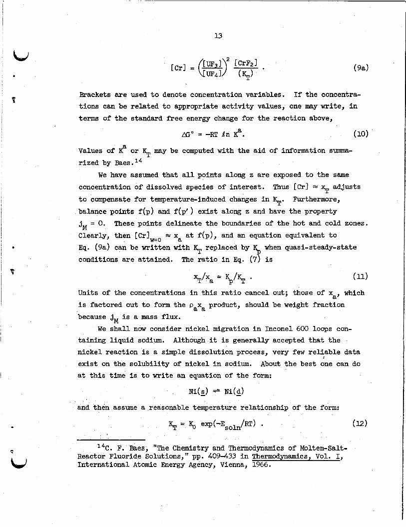
Brackets are used t o denote concentration variables. If the concentra- t ions can be related t o appropriate act ivi ty values, one may write, i n terms of the standard f ree energy change for the reaction above,

N O = -RT an e. (10)

Values of rized by Baes.14

or I$ may be computed w i t h the aid of information summa-

We have assumed that a l l points along z are exposed t o the same concentration of dissolved species of interest . Thus [ C r ] = 3 adjusts

t o compensate for temperature-induced changes i n I$. Furthermore, balance points f(p) and f(p' ) exist along z and have the property

= x a t f (p) , and an equation equivalent t o = 0. These points delineate the boundaries of the hot and cold zones. jM

Clearly, then [ C r ]

Eq. (sa) can be written with I$ replaced by K when quasi-steady-state conditions are attained. The r a t io i n Eq. (7) is

-0 a

P

Units of the concentrations i n this r a t io cancel out; those of xa, which i s factored out t o form the paxa product, should be weight fraction because j i s a mass flux. M

We shall now consider nickel migration i n Inconel 600 loops containing l iquid sodium. nickel reaction i s a simple dissolution process, very few rel iable data exis t on the solubi l i ty of nickel i n sodium. About the best one can do a t this time i s t o write an equation of the form:

Although it i s generally accepted that the

Ni(2) == Ni(d) and then assume a reasonable temperature relationship of the form:

I$ = K, . 1 4 C . F. Baes, "The Chemistry and Thermodynamics of Molten-Salt-

Reactor Fluoride Solutions," pp. 409-433 i n Thermodynamics, Vol. I, International Atomic Energy Agency, Vienna, 1966.

u

Values for K, and Esoh used i n the present report are, respectively, 6.794 x weight fraction and 6.985 kcal/mole. With these values Eq. (U), cast i n the form of Eq. (9), passes through a set of solubi l i ty data reported by Singer.15 It i s clear that

yr = YIYX , 03)

where we assume the ac t iv i ty coefficient 7 t o be unity and the mole fraction of nickel t o be unity, since the solubi l i ty experiments were conducted i n a pure nickel pot.16 i n the pot experiments) i s equivalent t o the experimental $. loop, x = (%/ma)Y/%.

what reaction E In certain ideal cases, Esoh would be nearly equivalent t o the heat of

fusion of nickel (= 4 kcal/mole), but i n the present case the solubilL- t i e s are so low and the data are so scattered it would seem d i f f i cu l t t o

attach definite physical significance t o t h i s variable. hot-to-cold-zone transfer requires the energy term t o be positive. it i s negative, material would tend t o move from the cold t o the hot zone.

In t h i s case, Y ( the saturation value

Thus once again the form of Eq. (11) holds true. In a

We might point out by way of conclusion that we real ly don't know

represents, as we did for the fluoride case, Eq. (10). soln

Note also that If

React ion Rates

Consider an alloy with constituent M that tends t o undergo a revers- ible solution reaction governed by a positive solution energy - namely,

kl

k2 M ( s ) M(g) .

iJ

t

"R. M. Singer and J. R. Weeks, "On the Solubility of Copper, Nickel, and Iron i n Liquid Sodium," pp. 309-318 i n Proceedings of the International Conference on Sodium Technology and Large Fast Reactor Design, November 7- 9, 1968, -7520, Part I.

dissolved nickel i n the saturated solution with the concentration expressed as ppm (by weight). A more conventional choice would have been t o express Y i n terms of mole fraction such that the corresponding ac t iv i ty would be unit a t sahra t ion . "his choice would have avoided a "spli t" definit ion of K , which appears later.

I6We have written Eq. (l3) i n terms of a selected standard s t a t e for 5

- LJ 7

hi .

As stated ear l ie r the symbols (s) - and (d) - denote the respective s ta tes solution i n the alloy and solution i n the liquid. One may se t for th the classical r a t e expression for the net amount of Mthat reacts i n terms of the molecular or atomic flux as F

a a JM = k1 'M(2) - k2 'M(d-)

54 The units of ka must take on those of JM (mole m u s t be dimensionless according t o established conventions. cm2 refer t o a uni t or peripheral area along z.

sec-l) because The units

A t equilibrium, J = 0, and one obtains the correct thermodynamic M expression for the equilibrium constant, which i s

Although Eqs. (U) and (15) are c lassical expressions - i n a thermodynamic sense - for first-order reactions, they seldom appear i n th i s form i n corrosion practice. the concentrations and equilibrium constants involve weight or mass fractions. Furthermore, the constants usually have velocity units. These conventions require the use of mass density terms. Therefore, additional modifications of Eqs. (14) and (15) are clearly i n order.

It i s convenient for present purposes t o take aM as the product

Mass fluxes are most frequently used, and c t

of an ac t iv i ty coefficient and the mole fraction. Then

c

W

where t ively.

and 7 represent mole fractions i n the solid and liquid, respec- Now i f new r a t e constants a re defined such that ,

then the expression for the mass f lux becomes

16 -

The superscr iptoappears as a reminder that the l iquid concentration L) that governs the dissolution reaction i s the value that exis ts between the metal and mass transfer film.

h -+ m, w i t h j, = 0 (equilibrium); then between K

Assuming the absence of a film, -

-+ Y, and the relationship I

and Ka may be readily found. It turns out that exp

Notice that the units of k, and k, are cm/sec.

Mass Transfer Across Liquid Films

The accepted and usual approach fo r explanations of the mass- transfer phenomenon i s t o invoke the close analogies that exis t for various modes of heat and mass transfer. In this case we are interested i n the mass-transfer analog of heat t ransfer as it occurs under Newton's l a w of cooling. write,

In terms of the concentrations i n the liquid, one may

and if surface reactions are fast - k, = k l / n > h -

The interested reader i s referred t o discussions given by Bird e t a1.17 O f particular importance is the analogous way i n which h's fo r mass and heat t ransfer are c0mputed.l' a diffusion parameter because a binary diffusion coefficient ( for example, Ni(d) i n sodium) appears i n the correlations concerning h fo r mass transfer.

Many think of h as a representative of

17R. B. B i rd , W. E. Steward, and E. N. Lightfoot, Transport

181bid., pp. 636-647, 681. Phenomena, pp. 267, 522, Wiley, New York, 1960.

I

17

4

c

W

Combined Reaction Rate-Film Resistances

In some instances, a complete description of surface effects may require coupling of the effects of both chemical kinetics and l iquid film transport such tha t the associated resistances t o f l u w ac t i n series. t o gain generality and completeness. tance i s a most important aspect of the following presentation regarding corrosion i n liquid-metal systems.

The relationships sought are not new.19 We repeat them here We note that the coupled resis-

Since a large portion of the combined surface effects involve l iquid behavior, we shall develop a r a t e term that gives the w a l l - related input t o an increment of f luid passing a unit area of w a l l . This term w i l l be altered t o conform t o solid-state diffusion convention by changing cer ta in l iquid concentrations t o pseudo-wall concentrations. Three reference concentrations, each referred t o the liquid, are involved. These are: Y, y , and y. Consider a unit area i n the hot zone. The same j

reaction-rate equation,

0 passes both the resistances associated w i t h the M

and the f i l m equation,

0 Thus, one m y solve for y using Eq. (20), substi tute th i s resu l t i n Eq. (181, and, using manipulations alluwed by Eq. (19), obtain:

where

lb = l/h + l/k2 . (22)

19J. Hopenfeld and D. Darley, Dynamic Mass Transfer of Stainless S tee l i n Sodium under High-Heat-Flux Conditions, NAA-SR-12447 (July 1967 1.

18

Surface Effects Referred t o the Alloy

The next point t o consider is the application of Eq. (21) t o solve a solid-state diffusion problem. follows with Y = I$x

Equation (21) may be al tered as + .

The superscript 0 appears on the x as a reminder tha t t h i s i s a t rue alloy concentration a t the surface. fo r subscript exp. (experimental) as a reminder that k = % varies with temperature. one t o treat y as independent of temperature. If .we are at a balance point, j =Q, 9 = g, and I$ = K , where subscript p denotes balance

point. Thus, y = K

may write

We have a l so substituted subscript T

exp A basic assumption stated i n the Introduction permits

M P and for a l l other points along z other than p we

P a'

where

xo= x K /% . " P

u I

Before writing dam the f i n a l forms, one w i l l r e c a l l tha t Eqs. (21) through (21b) were s e t up i n terms of posit ive f l a w in to a salt volume. This i s opposite t o the direction of f l a w in to the metal, so the sign of Eq. (21b) m u s t be reversed. Then,

w o , t > aw j, = -Dpa = gK(ma/%) (xo - x*)Pa

The surface condition can be set for th i n terms of a derivative

?

where

t

L

W

19

The variable & i s t o be treated i n general as x, so we s h a l l drop the

superscript 0 i n Eq. (241, from t h i s point on. It i s of some interest t o note that, if k, i n Eq. (17) had been defined as k2a*YM(d)%/ma,

Eq. (18) would have involved only weight fractions and the Fatio ma/%

would not have appeared i n Eq. (25).

TRANSIENT SOLUTIONS

The Introduction s ta ted tha t the loop operation was t o be initiated

with the y corresponding t o the quasi-steady state. Quasi-steady s t a t e invokes two conditions: and, hence, the concentration of surface elements, x(O,t), remain fixed with time, and (2) tha t the effects of the l iquid film resistance on mass t ransfer remain fixed with time. F’romthe resul ts of Report I, we conclude tha t the bulk concentration of the l iquid w i l l have a constant value i n some small f ract ion of an hour. We nuw wish t o examine the

point i n time tha t the second transient condition, &- x* f f ( t ) , w i l l be realized.

(1) tha t t he bulk concentration of the l iquid

To find the answer, we m u s t solve a somewhat complicated solid-state diffusion problem.

Review of the Equations

A succinct statement of the problem i s as folluws: Firs t , f ind a solution, x(w,t), of the Fourier equation,

J (26) 1 ax - f - -

ad D a t

incorporating Eq. (24) and other appropriate boundary conditions; then

manipulate the resul ts t o produce an expression l i ke Eq. (7). Solutions for Eq. (26) with (24) have been given for the hot

zones2’ using classical techniques, and for the cold zone alone2I using

S. C a r s l a w and J. C. Jaeger, Conduction of Heat i n Solids, 2nd ed., pp. 70-73, Oxford University Press, New York, 1959.

211bid., - pp. 305-306.

20

L3 Laplace transforms. We could start with these results; however, l i t t l e

would be gained and complete familiari ty would be lo s t i f this approach were followed. beginning, since the f lux expressions turn out t o be the same ( w i t h the

exception of different signs) fo r both zones. res t r ic ted t o one zone, and we shall choose the cold zone. Boundary conditions are x(w,O) = xa, x(w,t) = xa, x ( 0 , ~ ) = Xn; finally, X(O,t) must satisfy Eq. (24). Let

In fact , it is just about as easy t o start from the

Attention may be

t

and

We have

t o be solved w i t h t he boundary conditions:22

@(w,O) = 0 , (a)

@(0,4 = Ax!+ , (c>

@(-,t) -+ 0 , (b)

and

Notice that nothing i s said about & a t this point.

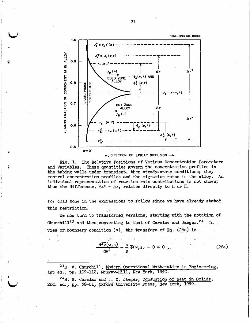
Figure l p r e s e n t s the variables involved for both the simple con- s tant potential and the present problems. We shall not use the subscript c

22With the variable change indicated, the solution for the concen- t ra t ion prof i le could be written i n a form analogous t o Eqs . (1) and (2); of course aXn would replace Ax. bypassed i n passing direct ly t o the expression for AM(t)/AZ.

It turns out that th i s solution w i l l be c

Ld

21

ORNL- O W 0 69- I0089 b,

'i

I I / .

L

hp,

1.0

>- 0 2 < 0.9 z I I- z % 0.8 2 8 I

LL 0

F 0.7

V

LL

v) v) 4 0.6 z

s

*

0.5

j,,, ( t)

COLD ZONE ALLOY - - w

v ) -

nIX $ 2

2 HOT ZONE

ALLOY -

I

AND

.--. - x g = 1 Ax

Ax*

--I. Ax"

w = o w , DIRECTION OF LINEAR DIFFUSION -

Fig. 1. The Relative Positions of Various Concentration Parameters and Variables. the tubing w a l l s under transient, then steady-state conditions; they control concentration profiles and the migration rates i n the alloy. individual representation of reaction r a t e contributions i s not shown; thus the difference, fW -Ax, re lates direct ly t o h or E.

These quantities govern the concentration profiles i n

An

for cold zone i n the expressions t o follow since we have already stated t h i s res t r ic t ion.

We now turn t o transformed versions, s tar t ing with the notation of C h ~ r c h i l l ~ ~ and then converting t o that of Carslaw and Jaeger.24 view of boundary condition (a), the transform of Eq. (26a) i s

In

23R. V. Churchill, Modern Operational Eilathermtics i n Engineering,

24H. S. C a r s l a w and J. C. Jaeger, Conduction of Heat i n Solids, 1st ed., pp. 109-112, McGraw-Hill, New York, 1950.

2nd. ed., pp. 5841, &ford University Press, New York, 1959.

22

where

The general solution of Eq. ma) i s

where q = (S/D)I/~.

derivative of the particular solution with respect t o w i s

To sa t i s fy condition (b), c2 must be zero. The

4 - V ( W , S ) = -qcle .

A t the surface,

S(0,s) = c1 ¶ 7' (0,s) = -qCl . Thus the transform of Eq. (24a) evaluated a t w = 0 i s

?((O,S) = H[T(O,s). - M / s l . This may be rewritten as

whereby

The inverse of @(w,s) = c,e- w i l l demonstrate that condition (c ) is sat isf ied. Xn + & i n view of the associated film condition (a).

This implies that aXn +Ax as t + 0 3 . In other words,

Now, since

it i s clear tha t

c

23

c 1

e

c

,

c

h*i

The s ta ted goal is a form l ike Eq. (7). In transformed coordinates this will be

Thus

(27)

The inverse25 transform of Eq. (27) i s

To go back t o sign conventions associated w i t h the corrosion medium, we

merely reverse signs by redefining aXn t o be

Equation (23) was used t o write the last form. Comparison of the first term of Eq. (27a) - including the new ver-

sion of M - w i t h the r ight side of Eq. (7 ) reveals tha t both forms a re equivalent. One may r eca l l that Eq. (7) was developed on the basis of negligible film or surface effects, whereby &d e. happens over a period of time, depending on the H value, because exp(-u2) erfc(u) -+ 0 as u - 0 ( t + O ) .

forming the r a t i o of &Az (where H i s accounted) t o AM/A, (where H i s

neglected). The r a t i o is:

This actual ly

Clarification i s gained by

25The inversion formula i n t h i s case i s tabulated as item 15, Appendix V, p. 405, i n H. S. C a r s l a w and J. C. Jaeger, Conduction of Heat i n Solids, 2nd. ed., Oxford University Press, New York, 1959.

24

Several somewhat fortuitous distinctions evolve when the results are put for th as a rat io . l m h u s a remainder; the remainder obviously fades out as time increases. This clearly demonstrates that surface effects, re la t ive t o diffusive effects, a re inportant only i n the i n i t i a l phases of the loop operation. An a t t rac t ive feature of Eq. (28) is the cancellation of M.

means that specification of the balance point (manifest through K ) i s not required t o prepare a p lo t shuwing the effects of h or H.

reader w i l l discover i n later sections that determination of the balance points is an involved procedure, even under quasi-steady-state conditions. Furthermore, we have no idea as t o where the balance points reside a t various times during the transient period. Thus, elimination of K con-

s t i t u t e s an important simplification at this point i n the report. M i s l o s t or gained by the alloy makes no difference when the r a t i o is used.

The results come out i n compact form as

This

P The

P Whether

The plots of the r a t i o versus t i m e are always positive.

Application t o Sodium- Inconel 600 Systems

For demonstrative purposes, we have concocted an i l l u s t r a t ive example fo r the Inconel-sodium system shawing rates and degrees of approach t o equilibrium, assuming that the only surface effects of importance are those associated w i t h the l iquid f i l m .

assume that k2 + m; thus 6 + h.

exis ts as t o the values of k, and k2 for the system. of % are not above question. la te r . mum and minimum temperatures for experiments w i t h Inconel 600 loops containing sodium, namely, 1089°K ( l5OO"F) and 922°K (1200°F).

In other words, we This i s assumed because no information

In fact , the values Details of the computation of H are given

We have compared two values of H corresponding t o typical maxi-

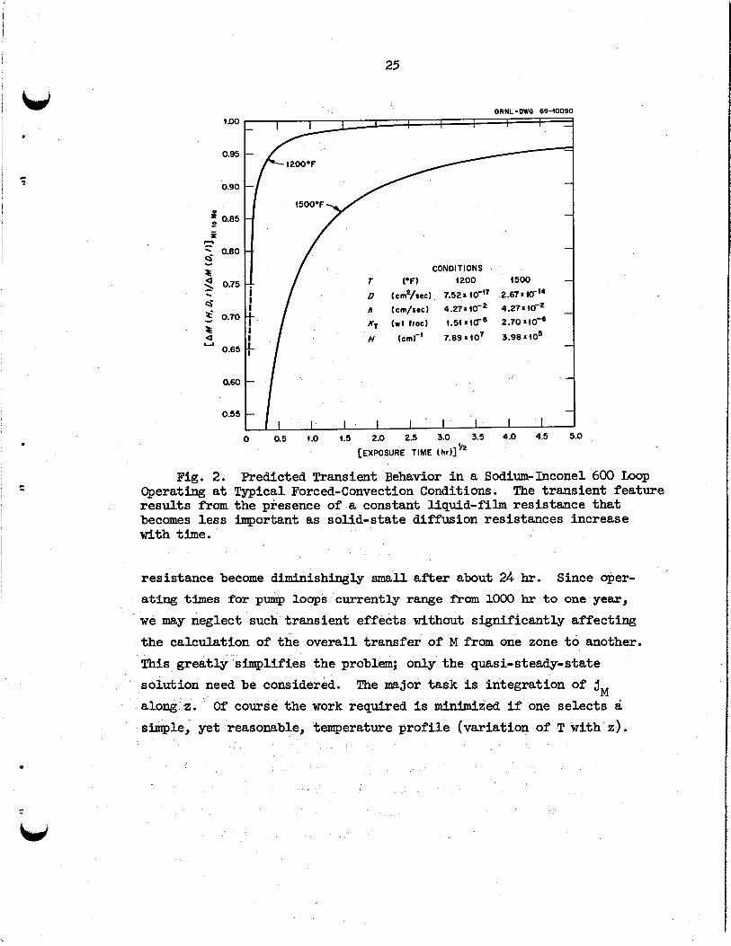
The example i s presented i n F i g . 2. Note that the film coefficient,

h, i n this example was assumed t o be the same at a l l surface points around the loop, while D and % i n H were assumed t o vary according t o the local l iquid (actually w a l l ) temperatures. curves c lear ly indicates that film coefficients are of greatest impor-

A comparison of these

tance i n the hot zone where solid-state diffusion ra tes are re la t ive ly high. Nevertheless, transient effects associated w i t h the liquid-film

I .

t

. I

i

25

ORNL-DWG 69-40090 4 . 0 0

0.95

c

0.90

0

f 0.85 L - z c . 0.80 a' 1

a 3 0.75 . 6 5 0.70

2 U

0.65

0.60

0.55

I I I I I I i I

i I

F I ' I I

-

-

- CONDITIONS

D {cm2/rec) 7.521 40-'7 2.67146'4

h (cm/rec) 4 . 2 7 ~ 4 4 ~ 4.27.40-2 - K, (ut froc) 1.54 14C6 2.70.10-6

H (crn)-' 7.89at07 3.98140' -

T 4200

D {cm2/rec) 7.521 40-'7 2.67146'4

h (cm/rec) 4 . 2 7 ~ 4 4 ~ 4.27.40-2

K, (ut froc) 1.54 14C6 2.70.10-6

H (crn)-' 7.89at07 3.98140'

0 0.5 4.0 t.5 2.0 2.5 3.0 3.5 4.0 4.5 5.0

[EXPOSURE TIME (hr)Ih t

Fig. 2. Predicted Transient Behavior in a Sodium-Inconel 600 Loop c + Operating at Typical Forced-Convection Conditions. The transient feature

results from the presence of a constant liquid-film resistance that becomes less important as solid-state diffusion resistances increase with time.

resistance become diminishingly s m a l l after about 24 hr. ating times for pump loops currently range fkam 1000 hr to one year,

we may neglect such'transient effects without significantly affecting the calculation of the overall transfer of M from one zone to another.

Since ~ e r -

simplifies the problem; only the quasi-steady-state solution need be considered. along z. Of course the work required is minimized if one selects a simple, yet reasonable, temperature profile (variation of T with z).

The major task is integration of jM

26

TEMPERATURE PROFILES AND LOOP CONFIGURATIONS

. Reference and Prototype Loops

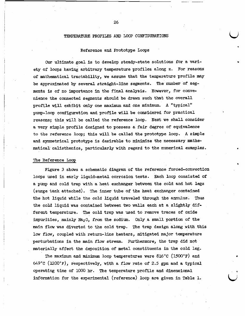
Our ultimate goal is t o develop steady-state solutions for a vari- ety of loops having arbi t rary temperature prof i les along z. For reasons

of mathematical t ractabi l i ty , we assume tha t the texperature prof i le may be approximated by several straight-l ine segments.

ments i s of no importance i n the f i n a l analysis. nience the connected segments should be drawn such tha t the overall prof i le wil l exhibit only one maximum and one minimum. A "typical"

pump-loop configuration and prof i le w i l l be considered for prac t ica l reasons; th i s w i l l be called the reference loop. a very simple prof i le designed t o possess a f a i r degree of equivalence t o the reference loop; t h i s w i l l be called the prototype loop. and symnetrical prototype is desirable t o minimize the necessary mathematical calisthenics, par t icular ly w i t h regard t o the numerical examples.

The number of seg-

However, for conve-

Next we s h a l l consider

A simple

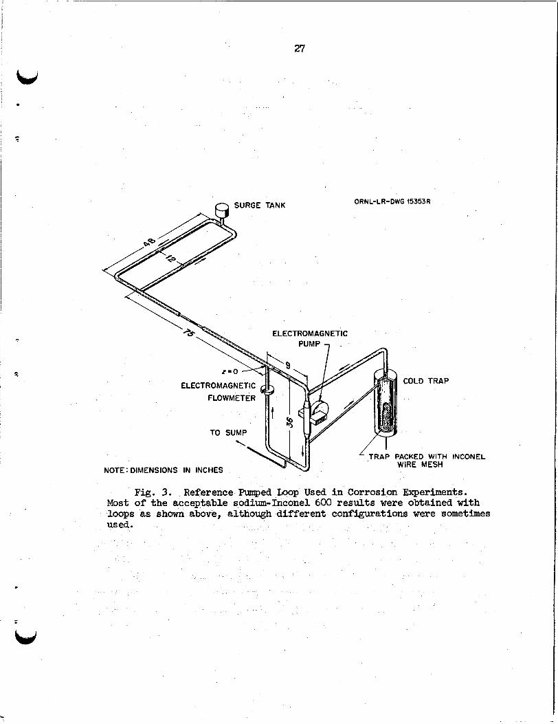
The Reference Loop

Figure 3 shows a schematic diagram of the reference forced-convection loops used i n early liquid-metal corrosion t e s t s . a pump and cold t rap with a heat exchanger between the cold and hot legs (surge tank attached). the hot l iquid while the cold l iquid traveled through the annulus. the cold l iquid was contained between two walls each a t a s l igh t ly dif-

ferent temperature. impurities, mainly Na20, from the sodium.

main flow was diverted t o the cold trap. l o w flow, coupled w i t h return-Pine heaters, mitigated major temperature

perturbations i n the main f low stream. materially affect the deposition of metal constituents i n the cold leg.

The maximum and minimum loop temperatures were 816°C (1500°F) and

Each loop consisted of

The inner tube of the heat exchanger contained

Thus

The cold t rap was used t o remove traces of oxide

Only a small portion of the The trap design along with t h i s

Furthermore, the trap did not

649°C (1200°F), respectively, w i t h a f l o w r a t e of 2.5 gpm and a typical

operating time of 1000 hr.

information for the experimental (reference) loop are given i n Table 1.

The temperature prof i le and dimensional

27

1

L -

L

ORNL-LR-DWG 15353R SURGE TANK

ELECTROMAGNETIC

ELECTROMAGNETIC

e ‘TRAP PACKED WITH INCONEL

WIRE MESH NOTE : DIMENSIONS IN INCHES

F i g . 3. Reference Pumped Loop Used i n Corrosion Experiments. Most of the acceptable sodium-Inconel600 resul ts were obtained with loops as shown above, although different configurations were sometimes used.

28

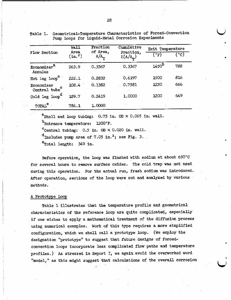
Table 1. Geometrical-Temperature Characteristics of Forced-Convection Pump Loops f o r Liquid-Metal Corrosion Experiments

Wall -action Cumulative Exit Tqerat.e

(OF) ( O C )

Flaw Section Area of Area, Fraction, ( in .2) A'% w4-J -

Economizer a 263.9 0.3367 0.3367 U50b 788

Hot leg loopa 222.1 0.2832 0.6197 I500 816

Economizer 108.4 0.1382 0.7581 1230 666

Annulus

Central tubeC

TOTALe 784.1 1.0000

Cold leg loopd l89.7 0.2419 1.0000 I200 649

i .

Shell and loop tubing: 0.75 in . OD X 0.065 in. wall. a

bEntrance temperature: 1200°F.

dIncludes pump area of 7.05 in.2; see Fig. 3. e

Central tubing: 0.5 in. OD X 0.020 in. wall. C

Total length: 349 in .

Before operation, the loop was flushed with sodium a t about 650°C for several hours t o remove surface oxides. during th i s operation. After operation, sections of the loop were cut and analyzed by various methods.

The cold t rap was not used

For the actual run, fresh sodium was introduced.

A Prototype Loop

Table 1 i l lu s t r a t e s that the temperature prof i le and geometrical characterist ics of the reference loop are quite complicated, especially if one wishes t o apply a mathematical treatment of the diffusion process using numerical examples. configuration, which we sha l l c a l l a prototype loop. designation "prototype" t o suggest tha t future designs of forced-

convection loops incorporate less complicated f l a w paths and temperature

prof i les . ) "model," as t h i s might suggest tha t calculations of the overall corrosion

Work of t h i s type requires a more simplified (We employ the

As stressed i n Report I, we again avoid the overworked word

a

29

V ra te , nM(t), depend on the f l o w characterist ics of the prototype. Except for transients, which are handled i n these reports, the solid- s t a t e diff 'uion mechanism depends only on the w a l l temperature and the concentration of dissolved alloy chnstituents. We care nothing about P

the f l o w i t s e l f or i t s direction.

*

L

Our purpose here i s t o propose a simplified configuration whereby a l l the geometrical complexities engineered in to early forced-convection loops w i l l be removed; yet the features important t o the mechanism under t e s t w i l l be retained. Actually, we are s t r iving for a maximum degree of equivalence between the reference and prototype loops. The most logical prototype tha t i s easi ly envisioned i s the "tent-shaped" prof i le over a constant-diameter loop used by Keyes.26 shaped" prof i le appears t o display the u t i l i t y desired, although it is somewhat awkward when applied t o other mechanisms, where perhaps a sawtooth prof i le might be most appropriate. prof i le composed of two straight-l ine segments cannot be experimentally obtained has been dispelled by DeVan and Sessions.27 that were tent-shaped but showed some asymmetry.

This "tent-

The idea that a tent-shaped

8 They used prof i les

1 In long-term pwnp loop experiments we sha l l eventually establish

r

W

t ha t liquid-film contributions are not of great importance; thus, the primary consideration is acquisition of a loop with an equivalent area. In Table 1 we see tha t the t o t a l area exposed t o l iquid is 784 in.2 or 5050 cm2. If we assume a constant diameter of 0.70 in . a l l around the loop, the t o t a l length w i l l be 906 cm, which is not too far removed f r o m the actual value of 886 cm fo r the reference loop. Reynolds number, (NRe>, weighted according t o the fract ional areas involved, i s 5.06 X lo4.

Thus, we inquire as t o the (NRe) for the prototype loop.

The average

Based on

r' y DNi-Nay Vz, pa, and CI values of 0.89 a, 3.3 X cm2/sec,

J. J. Keyes, Jr., Some Calculations of Diffusion-Controlled

27J. H. DeVan and C. E. Sessions, "Mass Transfer of Niobium-Base

26

Thermal Gradient Transfer, CF-57-7-115 (July 1957).

Alloys ' i n Flowing Nonisotherml Lithium, " Nucl. Appl. z$ 102-109 (1967). -

4

30

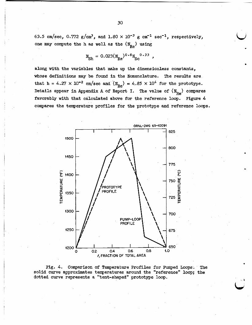
63.5 cm/sec, 0.772 g/cm3, and 1.80 X

one may compute the h as well as the ( NRe> using g cm'l sec'l, respectively,

0.33 Nsh = 0.023(NRe>0*8Nsc 9

along with the variables that make up the dimensionless constants, whose definitions may be found i n the Nomenclature. The resul ts a re that h = 4.27 X lo'* cm/sec and INRe> = 4.85 X lo4 for the prototype. Details appear i n Appendix A of Report I.

favorably with that calculated above for the reference loop. compares the temperature prof i les for the prototype and reference loops.

The value of (NRe> compares Figure 4

4 500

4450

c

& i400 W

3 a

a g 1350 G

5 c 4300

t 250

I200

, , , ORNL-DW,G 69-400; 825

Fig. 4. Comparison of Temperature Profiles for Pumped Loops. The sol id curve approximates temperatures around the "reference" loop; the dotted curve represents a "tent-shaped" prototype loop.

.

C

.

31

i

c

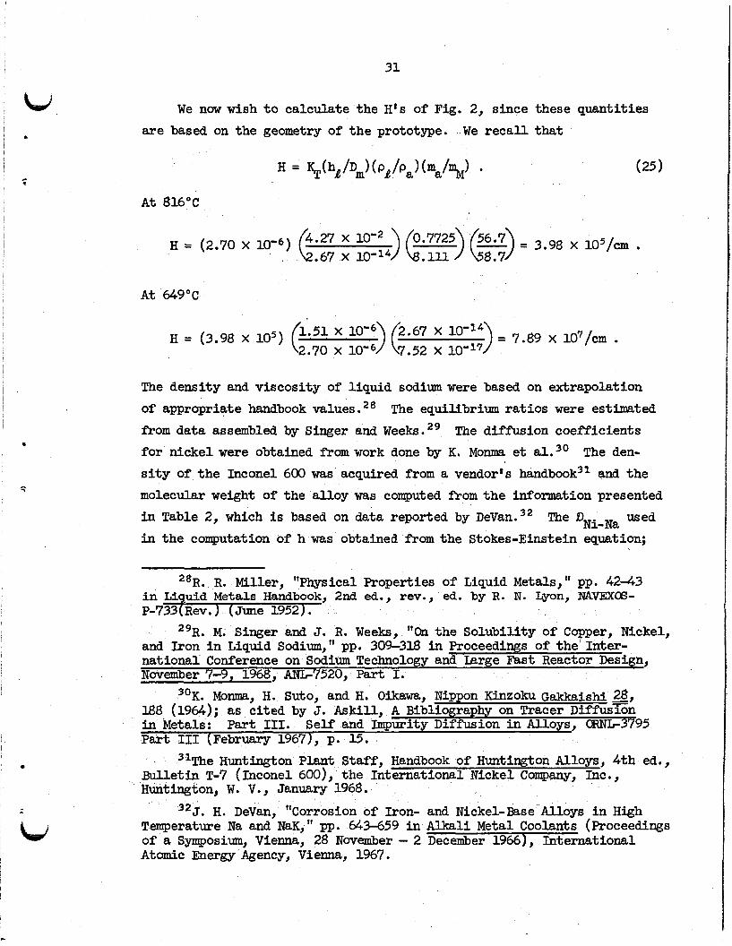
We now wish t o calculate the H's of Fig. 2, since these quantities a re based on the geometry of the prototype. We reca l l t ha t

H = (2.70 X log6) 6." ) f-z) = 3.98 X 105/cm . .6? X 1O-I" .1ll

A t 649°C

The density and viscosity of l iquid sodium were based on extrapolation of appropriate handbook values. 28

from data assembled by Singer and Weeks.29 The diffusion coefficients for nickel were obtained from work done by K. Monma e t aL3' The den- s i t y of t he Inconel 600 was acquired from a vendor's handbook3' and the molecular weight of the alloy was computed fromthe information presented i n Table 2, which is based on data reported by DeVan.32 in the computation of h was obtained fromthe Stokes-Einstein eqwtion;

The equilibrium ra t ios were estimated

The DNi-Na used

28R. R. Miller, "Physical Properties of Liquid Metals," pp. 4 2 4 3 i n Liquid Metals Handbook, 2nd ed., rev., ed. by R. N. liyon, "EX(X- P-733(Rev.) (June 1952).

"R. M. Singer and J. R. Weeks, "On the Solubili ty of Copper, Nickel, and Iron i n Liquid Sodium," pp. 30%318 i n Proceedings of the Inter- national Conference on Sodium Technology and Large Fast Reactor Design, Navember 7-9, 1968, -7520, Part I.

30K. Monma, H. Suto, and H. Oikawa, Nippon K i n Z O k u Gakkaishi 28, 188 (1964); as cited by J. AsM11, A Bibliography on Tracer Diff'usGn i n Metals: Par t 111. Self and Impurity Diffusion i n Alloys, ORNL3795 Part I11 (February 19671, p. 15.

31The Huntington Plant Staff, Handbook of Huntington Alloys, 4 th ed., Bulletin T-7 (Inconel 600), the International Nickel Company, Inc., Huntington, W. V., January 1968.

32J. H. DeVan, "Corrosion of Iron- and Nickel-Base Alloys i n High Temperature N a and NaK, I f pp. 643459 i n Alkali Metal Coolants (Proceedings of a Symposium, Vienna, 28 November - 2 December 1966), International Atomic Energy Agency, Vienna, 1967.

32

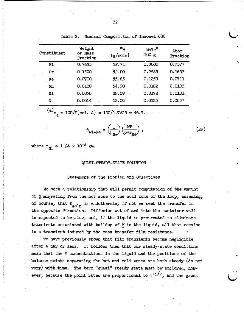
Table 2. Nominal Composition of Inconel 600

Weight 9 4 Molea Atom (g/mole) 100 g Fraction Constituent or Mass

Fractiun N i 0.7635 58.71 1.3000 0.7377

C r 0.1500 52.00 0.2885 0.1637

Fe 0.0700 55.85 0.1253 0.07ll rn 0.0100 54.90 0.0182 0.0103 S i 0.0050 28.09 0.0178 0.0101 C 0.0015 12.00 0.0125 0.0057

= lOO/C(col. 4 ) = 100/1.7623 = 56.7. a

where r = 1.24 x low8 cm. N i

QUASI- STEADY- STATE

Statement of the Problem

SOLUTION

and Objectives

We seek a relationship that w i l l permit computation of the amount of M migrating f'romthe hot zone t o the cold zone of the loop, assuming, of course, that Esoh i s endothermic; if not we seek the t ransfer i n

the opposite direction. Diffusion out of and in to the container w a l l i s expected t o be slow, and, if the l iquid i s pretreated t o eliminate transients associated with buildup of - M i n the liquid, a l l tha t remains i s a transient induced by the mass transfer film resistance.

We have previously shown that film transients become negligible a f t e r a day or less. mean that the - M concentrations i n the l iquid and the positions of the

balance points separating the hot and cold zones are both steady (do not

vary) w i t h time. The term "quasi" steady s t a t e must be employed, how-

ever, because the point rates a re proportional t o t+lI2, and the gross

It follaws then tha t our steady-state conditions

Li .)

33

a

,

c

8

t ransfer is proportional t o t-1/2. time integrals vary with t h e .

Therefore, both the rates and the i r Huwever, i n view of the quasi-steady-

s t a t e features of the problem, the time and position integrations may be performed independently of one another. This constitutes a great simplification of the tasks tha t l i e ahead.

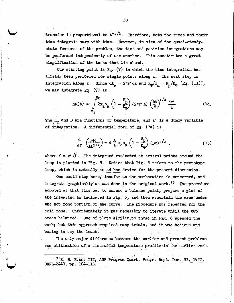
Our star t ing point i s Eq. (7) in which the time integration has already been performed fo r single points along z. integration along z. we may integrate Eq. (7) as

The next step is

Since dAz = 2flr’dz and %/xa = K p / S [Eq. (U)],

L

The % and D are f’unctions of temperature, and z‘ i s a dummy variable of integration. A di f fe ren t ia l form of Eq. (7a) i s

where f = z’ /L. loop i s plotted i n Fig. 5. loop, which is actually an -- ad hoc device for the present discussion.

integrate graphically as was done i n the original work.33 adopted at that time was to assume a balance point, prepare a plot of

the integrand as indicated i n Fig. 5, and then ascertain the area under the hot zone portion of the curve. The procedure was repeated for the cold zone. areas balanced. Use of plots similar t o those i n Fig. 6 speeded the work; but t h i s approach required many t r i a l s , and it was tedious and boring t o say the least .

The integrand evaluated a t several points around the

Notice tha t Fig. 5 refers t o the p r o t o t h e

One could stop here, insofar as the mathematics is concerned, and

The procedure

Unfortunately it was necessary t o i t e r a t e u n t i l the two

The only major difference between the ear l ie r and present problems was ut i l iza t ion of a sinusoidal temperature prof i le i n the ear l ie r work.

33R: B. Evans I11 ANP Program Quart. Progr. R e p t . Dec. 31, 1957, oRNL2440, pp. 104-113.

i

34

ORNL-DWG 69-2953A

I I I I I I I I - 1080 ( 1 o-~)

12 -

n -- 10 - 0 Q, In c

'E 0 P, v

6 - 5 * 4 - s a 2 - W

klI2 0

-2

* i { CI Y

1060

I I I I I 1

I I I

t

~

-1040 e W K

-1020 = 5 a W - 1000 g W I- - 980 'J a 3 i 960 -

/ /

\

/ \ - 940 \

I /

I i~ I I 0 0.1 0.2 0.3 0.4 0.5 0.6 0.7 0.8 0.9 1.0

f , FRACTION OF WALL AREA AND/OR LOOP LENGTH

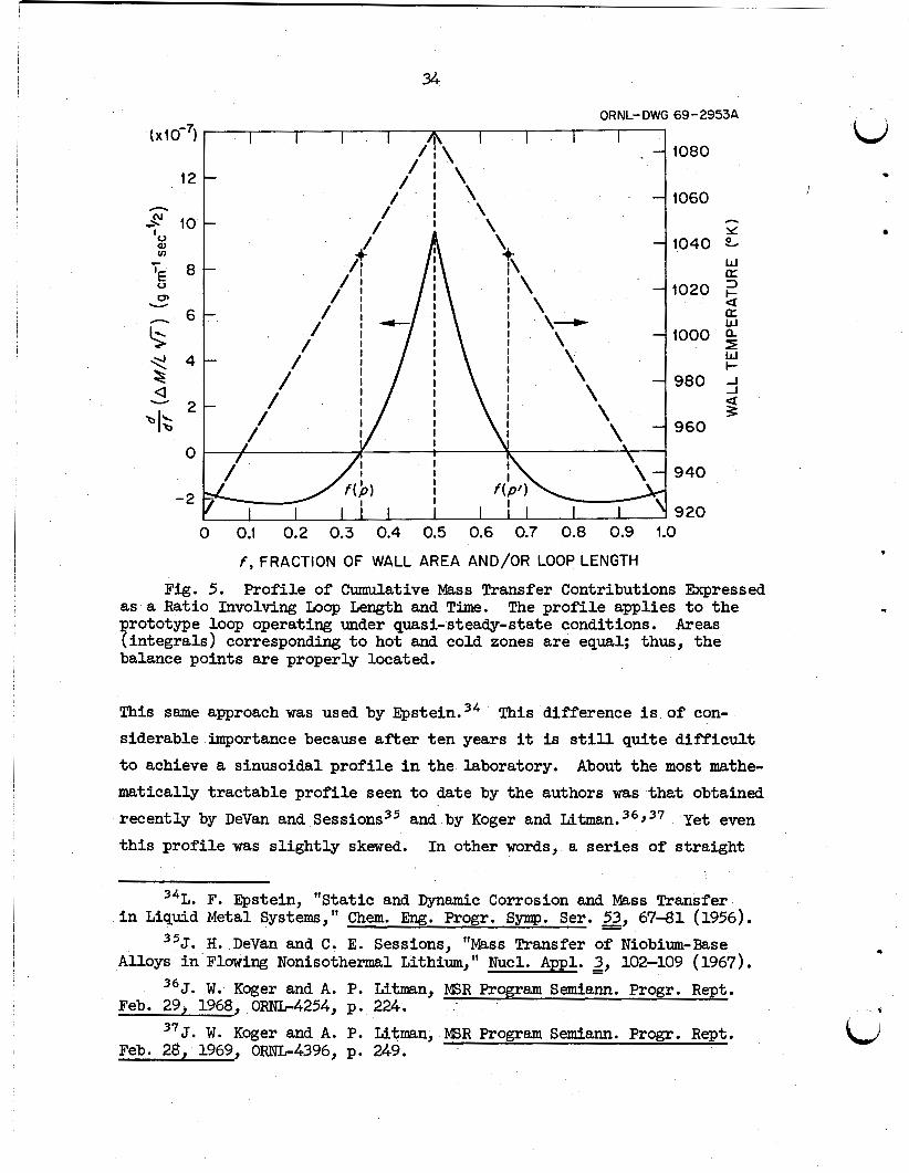
Profile of Cumulative Mass Transfer Contributions Expressed Fig. 5. as a Ratio Involving Loup Length and Time.

Areas ?integrals) corresponding t o hot and cold zones a re equal; thus, the balance points are properly located.

The prof i le applies t o the rototype loop operating under quasi-steady-state conditions.

This same approach was used by E p ~ t e 5 . n . ~ ~ siderable importance because a f te r ten years it is s t i l l quite d i f f i c u l t

t o achieve a sinusoidal prof i le i n the laboratory. About the most mathe- matically tractable prof i le seen t o date by the authors was t ha t obtained recently by DeVan and Sessions35 and by Koger and Litman.36,37 t h i s prof i le was s l igh t ly skewed.

This difference i s of con-

Yet even In other words, a ser ies of s t ra ight

34L. F. Epstein, "Static and Dynamic Corrosion and Mass Transfer

35J. H. DeVan and C. E. Sessions, "Mass Transfer of Niobium-Base i n Liquid Metal Systems, Chem. Eng. Progr. Symp. Ser. 2, - 6 7 4 1 (1956).

Alloys i n Flowing Nonisothermal Lithium," Nucl. Appl. 2, - 102-109 (1967). 36J. W. Koger and A. P. Litman, MSR Program Semiann. Progr. Rept.

37J. W. Koger and A. P. Iiitman, MSR Program Semiann. Progr. Rept.

Feb. 29, 1968, ORNL-4254, p. 224.

Feb. 28, 1969, ORNL4396, p. 249.

35

- *

TEMPERATURE (OF)

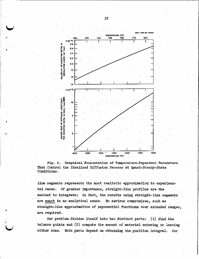
Fig. 6. Graphical Presentation of Temperature-Dependent Parameters That Control the Idealized Diffusion Process a t Quasi-Steady-State Conditions.

l i ne segments represents the most r e a l i s t i c approximation t o experimen- t a l cases. Of greater Importance, straight-l ine profiles a re the easiest t o integrate: a re exact i n an analytical sense. straight-l ine approximation of exponential functions over extended ranges, a re required.

balance points and (2) compute the aslount of material entering or leaving ei ther zone.

i n fact , the resul ts using straight-l ine segments No serious compromises, such as

Our problem divides i t s e l f in to two dis t inc t parts: (1) find the

Both parts depend on obtaining the position integral . Our

36

approach w i l l be t o carry out the manipulations using the prototype loop; present computations for the prototype loop using numerical examples, hopefully t o c la r i fy the overall procedure and nomenclature; and finally, discuss extension t o cases l ike the reference loop.

Solution i n Terms of the Prototype Loop

Equation (“a) is our starting point for the integrations that w i l l produce a solution

The reader w i l l r e ca l l that the time integration was performed ear l ier . A factor of 1/2 appears on the l e f t side as the symmetry of the ten t prof i le permits consideration of only half the loup. introdaced the expression for the diffusion coefficient i n the form of

Also we have

(D)I/’ = (Do)1/2 exp -E 2RT . ( 4 ) The equilibrium constant may be written similarly as ei ther

% = KO exp(-Esol, /RT) J

or

($1-1 = exp (+Esol, /RT)

Thus Eq. (7c) can be divided conveniently into two parts: , \

where

2RT J

U

c

.

37

and

C'= CK /K . P O

(33)

The next par t of the problem i s the key t o the whole solution. It

concerns the relationship between T and z. obvious relationship is

In terms of "C (or O F ) an

T(z) = Tc + bz , "C 9

where z runs from 0 t o 0.5; thus

b = 2(TH - Tc)/L = 2AT/L (34a)

This would be an ideal form if the exponential terms i n Eq. (7c) were

not present. of T expressed i n OK. f i l e s i n Fig. 5 whereby the distance 5 would be zero a t absolute zero (-273°C: or 0°K) .

r eca l l s the t r i v i a l relationship, AT( OK) = AT( "C), which means tha t k is valid for both temperature scales.

However, they a re indeed present; also they demand values Consider an extension of the segments on the pro-

What w i l l happen is not d i f f i cu l t t o visualize if one

One immediately envisions the poss ib i l i t i es of an extended coordinate k such tha t

k = (L/2AT)(273 + T°C) = b'l(273 + Tmin + A T ) ,

9 = k o + z , a, (35 1

which in turn simply means that we have adopted the relationship

.

T = b 5 , O K , (358)

for the extension. be introduced in to Eq. (7c) with this and follawing definitions:

From Eq. (35) dk = dz, and the new variable 6 may Let

(2 = Ej,/2bR (36)

and

38

Then the right side of Eq. (7d) becomes

or, in abbreviated form,

CIl2(a/E) - C' Il2(j /E) . We are now ready for integration. Whether one operates on the

urrprimed or primed term is of no consequence as long as a or a' > 1.

Thus we choose the former. th i s point.

However, a change of variable is userul a t L e t u = a/! or E = a/u; then dE = -(a/u2)du;

Integration i n terms of u can be performed by par ts with the formula

We l e t

then

A l s o we note that u + 03 as 8 + 0. The resul t is 3 3

U

39

Notice, v ia Eqs. (35a) and (36), that u = %/2RT in this case. the integration does not involve position - only temperature. L does enter the resul ts through the factor a. broken up into two parts, each with in f in i t e limits, t o cast the resul ts i n to a form that brings for th the so-called exponential integrals of the first order.

Clearly However,

The integral term was

These a re tabulated i n the l i terature .38 In our work,

values of the argument a re large, and in t h i s case the tabulations are i n the form

where

The 7 in this case is the dimensionless dummy variable of integration T = uf = C%/tf. One can shuw, using uf = a/(', that

m

J

The minus sign i s accounted for by suitable arrangement of terms. As

suggested by the form of the tabulated values, the f i n a l resu l t may be written as

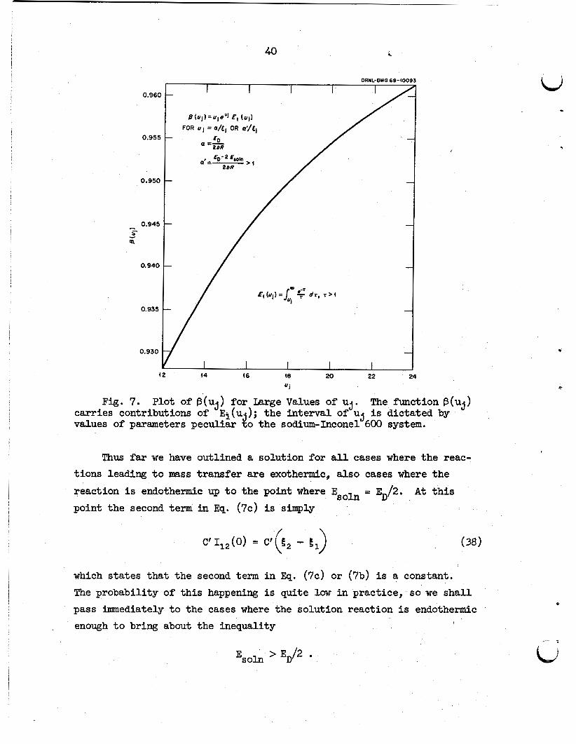
which clear ly shows the contribution of the position variables. Values of B(u ) a re plotted on Fig. 7. An accurate interpolation

of the values i s clearly required because the resul ts contain the dif-

ference 1 - @(u ), and B(u ) values are not too far removed from unity

3

3

38W. Gautschi and W. F. C a h i l l , "Exponential Integral and Related Functions," pp. 228-231 and p. 243 i n Handbook of Mathematical Functions, ed. by M. A b r d t z and I. A. Stegun, U.S. D e p t . of Commerce, NES publication M - 5 5 (June 1964).

40 1

0.960

0.955

0,950

0 . 9 4 5 - c - Q

0 . 9 4 0

0 .935

0.930

42 44 16 48 2 0 22 24

“i

Li

Fig. 7. Plot of f3(uj) for Large Values of u j . The function p(uj) carries contributions of El(u-); the interval of u j i s dictated by values of parameters peculiar 20 the sodium-Inconel 600 system.

Thus far we have outlined a solution for a l l cases where the reac- t ions leading t o mass t ransfer a r e exothermic, also cases where the

point the second term i n Eq. (7c) is simply

reaction i s endothermic up t o the point where Esoln = E#. A t this

which s ta tes that the second term i n Eq. (7c) or (7b) is a constant. The probability of this happening is quite law i n practice, so we sha l l pass immediately t o the cases where the solution reaction i s endothermic enough t o bring about the inequality 1

E s o h > ED/2 i

41

When the energy of solution overrides the contribution of the energy of activation for diff'usion, the second term in Eq. (7c) becomes

Note that C' remains the same.

same substitutions, one obtains the following: In terms of g coordinates, using the

where it may be he lp f i l t o think i n terms of the equality, a" = 4. Integration yields

which may be rearranged t o conform t o tabulated functions as

Collection and rearrangement of terms permits one t o write

where

and

The last function, E. (u ) i s the exponential integral; values of 1 3 - h(uj) appear i n the same tables38 as those for B(u ). The presence of 5

42

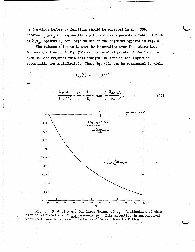
u1 functions before u2 functions should be expected i n Eq. (39b) because ul > ~2 and exponentials with posit ive arguments appear. of h(u ) against u . for large values of the argument appears i n Fig. 8 .

"he balance point i s located by integrating over the ent i re loop. One assigns 1 and 2 i n Eq. (7d) as the terminal points of the loop. A

mass balance requires tha t t h i s integral be zero if the l iquid is essentially pre-equilibrated.

A plot

3 3

Thus, Eq. (7d) can be rearranged t o yield

o r

i.i5

i.i4

Li3

i.i2

i.ii

6 i.io - 4

1.09

i.08

t.07

i.06

i.05

1 -\

I I I I I I I I I I I 9 (0 ii 12 13 (4 15 $6 47 48 19 20

ui

Fig. 8. Plot of A(uj) for Large Values of u . Application of t h i s plot i s required when 2ESoln exceeds ED. This si$uation is encountered when molten-salt systems are discussed i n sections t o follow.

43

ib, I

j ] i

L

One may back calculate t o find T and then successively z, f, tp, and finally, u . The AM may be evaluated by application of Eq. (7d) using

either the limits (1,p) over the cold zone or (p,2) Over the hot zone. Details concerning these manipulations appear i n the next section.

P

FVedicted Results for Sodium-Inconel 600 Systems

Two objectives are associated with t h i s section of the report. F i r s t , we hope t o attach some physical r ea l i t y t o equations developed i n the previous section through presentation of numerical examples, thereby demonstrating that the equations are easy t o use i n sp i te of t h e i r formidable appearance. Second, we desire t o predict corrosion

rates under our assumed condition tha t diffusion controls both i n the hot and cold zones and that a predictable balance point does exist , as suggested by the microprobe data shown i n Report I.

procedures for the preceding derivations, we may specialize t o the case of the prototype for simplicity without too much loss i n generality.

To pa ra l l e l the

One may start by considering the f irst and third columns of

Table 3. Eq. (34a):

The first computation required involves b. One finds, using

b" = L/2AT = 906/2 X 167 = 2.71 cm/"K . Related equations give

gl = (2.715 crn/'K)(922"K) = 2503 ,

and

E Z = (2 .7E cm/'K)(1089"K) = 2956 cm . Computation of u1 and u2 requires a knowledge of a and a'. i n turn, require parameters associated with the curves of Fig. 6.

But these,

4 4

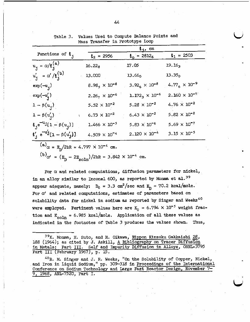
Table 3. Values Used t o Compute Balance Points and Mass Transfer i n Prototype Loop

t j , c m 5 k2 = 2956 E, = 28x6 E, = 2503 Functions of 5

u = a / l ( a ) 16. 228 17.05 19.163

= at /p ' 13.000 13.660 13.350 5 5

5 exp(-u.> 8.98, x 3.92, x 10-8 4.77, x

J 2.26, X lo', 1.172, X 2.160 X

1 - B(Uj) 5.52 X 5.28 X 4.76 X

5.82 X 1 - B(u;) \ 6.73 X 6.43 X

e 3 [ i - p(uj)] 1.466 X 5.83 X 5.69 x 10'~ 5 e t .i e-311- p(u>) 1 4.509 X 2.120 x 10'~ 3.15 x 10-5

= 5/2bR = 4.797 x loo4 a. (b)cz' = (ED - 2Esoln )/2bR = 3.842 X low4 cm.

For a! and related computations, diff'usion parmeters fo r nickel, i n an al loy similar t o Inconel 600, as reported by M o m e t al.,'

appear adequate, namely: For d and related computations, estimates of parameters based on so lubi l i ty data for nickel i n sodium as reported by Singer and Weeks4' were employed. t i on and Esoh = 6.985 kcal/mole. indicated i n the footnotes of Table 3 produces the values shown.

Do = 3.3 cm2/sec and = 70.2 kcal/mole.

Pertinent values here are = 6.794 X loo5 weight frac- Application of a l l these values as

Thus,

39K. Monma, H. Suto, and H. O i k a w a , Nippon Kinzoku Gakkaishi 28, 188 (1964); as c i ted by J. Askill, A Bibliography on Tracer Diff 'ussn i n Metals: Part 111. Part I11 (February 19671, p. 15.

Self and Impurity Diffusion i n Alloys, 0-3795

4 0 R . M. Singer and J. R. Weeks, "On the Solubili ty of Copper, Nickel, and Iron i n Liquid Sodium," pp. 309-318 i n Proceedings of the International Conference on Sodium Technology and Large Fast Reactor Design, November 7- 9, 1968, ANL7520, Part I.

L i .

.

E

45

, w

c

I

n

various values of g The l a t t e r allowed calculation of the exponential functions; they a l so

could be converted t o the corresponding u. values. 3 3

allawed acquisition of appropriate 1 - B(u ) values with the aid of enlarged versions of Fig. 7. a re positive; thus, functions related t o the El(u ) values apply here. The operations necessary t o complete the f i rs t and th i rd columns are straightforward and require no additional c m e n t .

balance points (the points at which j, = 0).

under consideration, j u s t one point i s needed because symmetry permits treatment of only half the loop. The cr i ter ion i s t o set m ( t ) = 0 i n

Eq. (7d). Thus the appropriate sum of the integral term must a lso be zero when the integration i s carried out over the en t i re loop. facet of the solution i s discussed around Eq. (40), reference t o which

clear ly indicates the method of approach; namely, we seek T or f (p) through K .

3 In t h i s regard, note t h a t both a! ando!

3

The next and perhaps most important task i s a computation of the Since the prototype i s

This

P The latter is given by:

P

The temperature corresponding t o K i s 1036°K; thus C = (2.715)(1036") P P

= 2813, and f (p) (of L/2) i s 0.683. middle column corresponds t o E

the cold zone (Umits: 1,p) and fo r the hot zone (limits: p,2).

Computation of the values i n the information.

Finally a value for AM(t) may be found by use of integral terms fo r P

Values fo r both zones were computed and averaged since a l l the differences involved introduced same uncertainties i n "hand calculations. " thing required t o calculate m ( t ) appears i n Table 3 except values of C

and Cf . The latter are evaluated through Eqs. (32) and (33). Thus

Every-

and

C' = (3.37 X 10'2)(70.9) = 2.39 . For the cold zone, using Eq. (7c) again,

46

AM(t)/2t1/2 = (70.9)(5.83 - 0.569) x 10'6 - (2.39)(2.12 - 0.315) x

3: (3.73 - 4.31) X = -5.8 x lo'* g / s d 2

For the hot zone,

AM(t)/2t1/2 = (70.9)(14.66 - 5.83) X loo6 - (2.39)(4.509 - 2.12) x

= (6.26 - 5.71) x = +5.5 X ' l O W 5 g/sec1I2 . The different signs mean that the l iquid sodium loses nickel i n the cold zone, but it gains nickel ( i n principle, an equal amount) i n the hot zone. The t e s t period of interest i s 1000 hr, 2t1/2 = 3.8 X sec1/2; therefor e :

m(t = 1000 hr) = (3.8 X 10+3)(5.65) = 0.215 g N i . A very high value of transport could be obtained by assuming that

no balance point would exist because a l l the l iquid could be forced through a 100$-efficient nickel t rap placed at the coldest point of the loop. In other words, the ent i re loop would be a hot zone. One obtains

AM/-(t = 1000 hr) = (3.8 X 1O3)(7O.9)(U.66 - 0.57) X lom6

= 3.8 g N i . This value was computed f o r comparative discussion.

DISCUSSION OF SODIUM-INCONEL 600 RBSULTS

The manner i n which the material has been presented up t o this

point almost demands that some camparisons be made between predicted

(computed) resu l t s for the prototype loop and those for the reference loop. mathematics t o actual loops with temperature prof i les as indicated by the sol id l ine segments i n Fig. 4 i s re la t ively simple i n principle, but tedious i n practice - because symmetry is lost and several straight-

l i ne segments (each w i t h i t s own b, a, and a' values) are present.

In t h i s connection, we digress t o note tha t extension of the

Of

Li

I,

47

bd 2

course, each must be accounted. developed t o handle a l l cases where E,, L 2Esoln.

justified. point is difficult t o determine precisely by hand; we might add that

acquisition of predicted corrosion and deposition prof i les i s a l so desired.

the computer can evaluate many "point" jM1s quite rapidly a f t e r locating the balance points [and evaluating AM(t) i n passing].

resul ts for the actual loop and the prototype are presented together. The 1000-hr AM(t)'s computed frm the integral forms are 0.232 g f o r the actual p ro f i l e and 0.213 g for the prototype. calculations based on Table 3 gave a value of 0.215 g for the prototype. The locations of the balance points for each case a re a l so i n close

Accordingly, a computer program41 was

There were several reasons whereby use of a program could be As sham i n our i l l u s t r a t ive calculations, the balance -

The program permits an accurate prediction of these because

The reader i s invited t o inspect Fig. 9, i n which computer program

Recall that the hand

agreement. device fo r estimating AM, even though the profiles themselves turn out t o be somewhat different i n appearance.

Thus we may conclude that the prototype i s an excellent

The point of greatest importance is whether or not the mechanism under discussion here gives a reasonable representation of what happens i n an experimental loop. f o r Report I, is, "No, it does not!"

ranges between 10 t o IA g N i .

ably less than 1 g N i i f one assumes that a balance point exis ts and

about 4 g if one assumes that the ent i re loop acts as a hot zone under the dominance of the mechanism proposed. probe data show that deposition occurs i n a t least half the loop. Deposition tendencies are, i n fact , so great that a region of nickel deposits appears, and f'urthermore samples of loop sodium suggest that

The answer t o the question, as was the case The amount we must account fo r

The computations produce values consider-

In regard t o the latter, micro-

the l iquid i s ei ther supersaturated or contains suspended metal particu- la tes a l l around the c i rcu i t . Thus we can forget 'about the value of

4xThe computer program was devised by D. E. Arnurius and V. A. Singletary of the Mathematics Division at ORNL. The authors acknowledge this important contribution t o the present study.

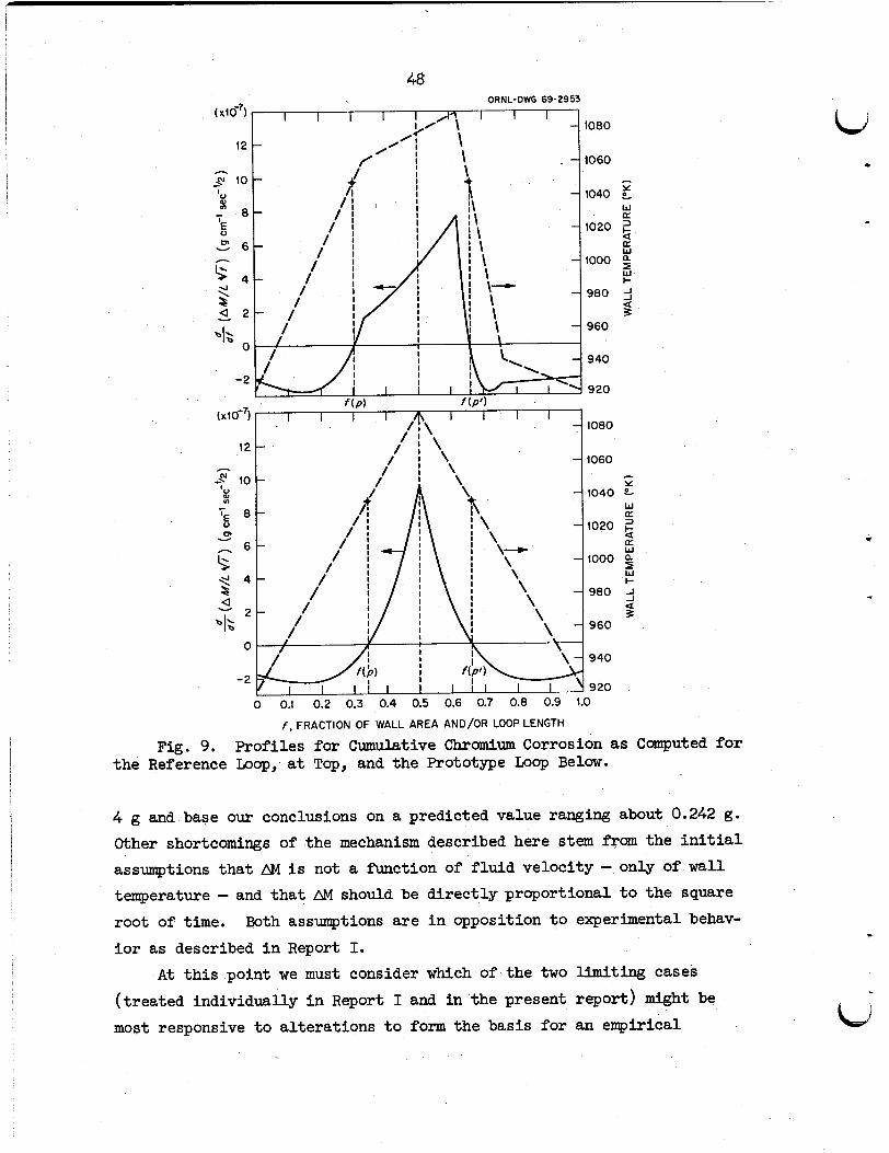
48 ORNL-DWG 69-2953

1080

1060 c Y

w 1040

a

a 1020 $

W

w I-

1000 2

980 5 a 3

960

940

920

f , FRACTION O F WALL AREA AND/OR LOOP LENGTH

Fig. 9. Profiles for Cumulative Chromium Corrosion as Computed f o r the Reference Loop, a t Top, and the Prototype Loop Below.

4 g and base our conclusions on a predicted value ranging about 0.242 g. Other shortcomings of the mechanism described here stem from the i n i t i a l assumptions tha t AM i s not a function of f lu id velocity - only of w a l l tempera.ture - and tha t AM should be direct ly proportional t o the square root of time. i o r as described i n Report I.

(treated individually i n Report I and i n the present report) might be most responsive t o alterations t o form the basis fo r an empirical

Both assumptions a re i n opposition t o experimental behav-

A t t h i s point we must consider which of the two limiting cases

.

49

correlation. In other words, if we were t o concoct a combined mechanism accounting solid-state and liquid-film diffusion effects together, where should we start? on thC liquid-film mechanism, simply because it i s the faster of the two considered thus far. resistances associated with a fast mechanism can always be reduced by addition of a time-variable resistance that acts i n series with the liquid film. decreasing the resistance of the slower mechanism. here tha t inclusion of a f i l m resistance i n the usual manner gives r i s e t o a transient effect, which decays with time. Although such an effect i s fortuitous, the overall resul t was t o reduce further the already low value of material transported.

Intuitively, we lean toward the idea of going t o work

We are attracted t o t h i s point of view because

On the other hand, it would be most d i f f i cu l t t o jus t i fy We should mention

Two possibi l i t ies for altering the diffusion mechanisms under dis-

cussion might seem feasible. value of D

would eoincide. t h i s might be tempered by the use of higher solubi l i ty values. Never- theless, increases of this magnitude do not appear reasonable, and one tends t o ru le out t h i s possibil i ty.

The first would involve increasing the such tha t the predicted resul ts and experimental data N i

The factor of increase would have t o be about lo3, but

A second possibi l i ty for increasing the predicted values w u l d be t o invoke solid-state diffusion equations where the point at which w = 0

moves around the loop. s l ight ly thicker i n cold regions and s l ight ly thinner i n the hot zones. This would accrue from corrosion reactions tha t w i l l not " w a i t for" a diffusion-controlled process. However, the solution x(w,t), even fo r the case where the w = 0 boundary moves a t a constant r a t e (a simple case),42 is too cmplex t o be effectively applied t o a makhematical treatment of the mass transfer process.

In other words, assume that the walls grow

"A solution of t h i s kind i s given by E. G. Brush, Sodium Mass Transfer; XVI. The Selective Corrosion Component of Steel Exposed t o Flowing Sodium, GW-4832 (March 19651, Appendix 11, pp. 105-110. More general forms of t h i s solution appear on pp. 388-389 of H. S. C a r s l a w and J. C. Jaeger, Conduction of Heat i n Solids, 2nd ed., Oxford University Press, New York, 1959, along with citations of the original work ( i n 1955), which also involved diffusion i n l iquid metals.

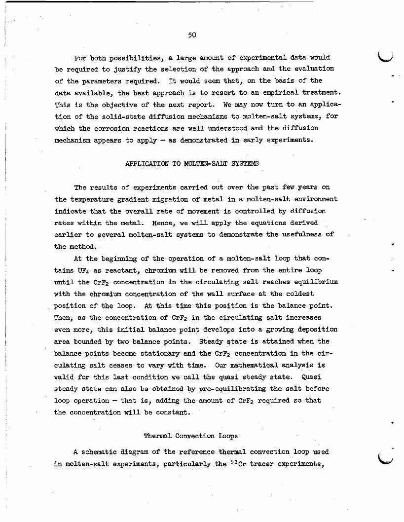
50

For both possibil i t ies, a large amount of experimental data would be required t o jus t i fy the selection of the approach and the evaluation of the parameters required. data available, the best approach i s t o resort t o an empirical treatment. This i s the objective of the next report. We may now turn t o an applica- t ion of the solid-state diffusion mechanisms t o molten-salt systems, fo r

It would seem that, on the basis of the

which the corrosion reactions are well understood and mechanism appears t o apply - as demonstrated i n early

APPLICATION TO MOLTEN-SALT SYSTEMS

the diffusion experiments.

The resul ts of experiments carried out over the past few years on

the temperature gradient migration of metal i n a molten-salt environment indicate tha t the overall rate of movement is controlled by diffusion rates within the metal.

ear l ie r t o several molten-salt systems t o demonstrate the usef'ulness of the method.

Hence, we w i l l apply the equations derived

A t the beginning of the operation of a molten-salt loop that con- ta ins Ul?4 as reactant, chromium w i l l be removed from the ent i re loop u n t i l the CrF2 concentration i n the circulating salt reaches equilibrium w i t h the chromium concentration of the w a l l surface a t the coldest position of the loop. Then, as the concentration of CrF2 i n the circulating salt increases even more, this i n i t i a l balance point develops into a gruwing deposition

area bounded by two balance points.

A t th i s time t h i s position i s the balance point.

Steady s t a t e i s attained when the balance points become stationary and the CrF2 concentration i n the circulating s a l t ceases t o vary with time. valid for this last condition we ca l l the quasi steady s ta te . steady state can also be obtained by pre-equilibrating the salt before loop operation - that is, adding the amount of CrF2 required so that the concentration w i l l be constant.

Our mathematical analysis i s Quasi

Thermal Convection Loops

A schematic diagram of the reference thermal

i n molten-salt experiments, particularly the 51Cr convection loop used t racer experiments ,

.

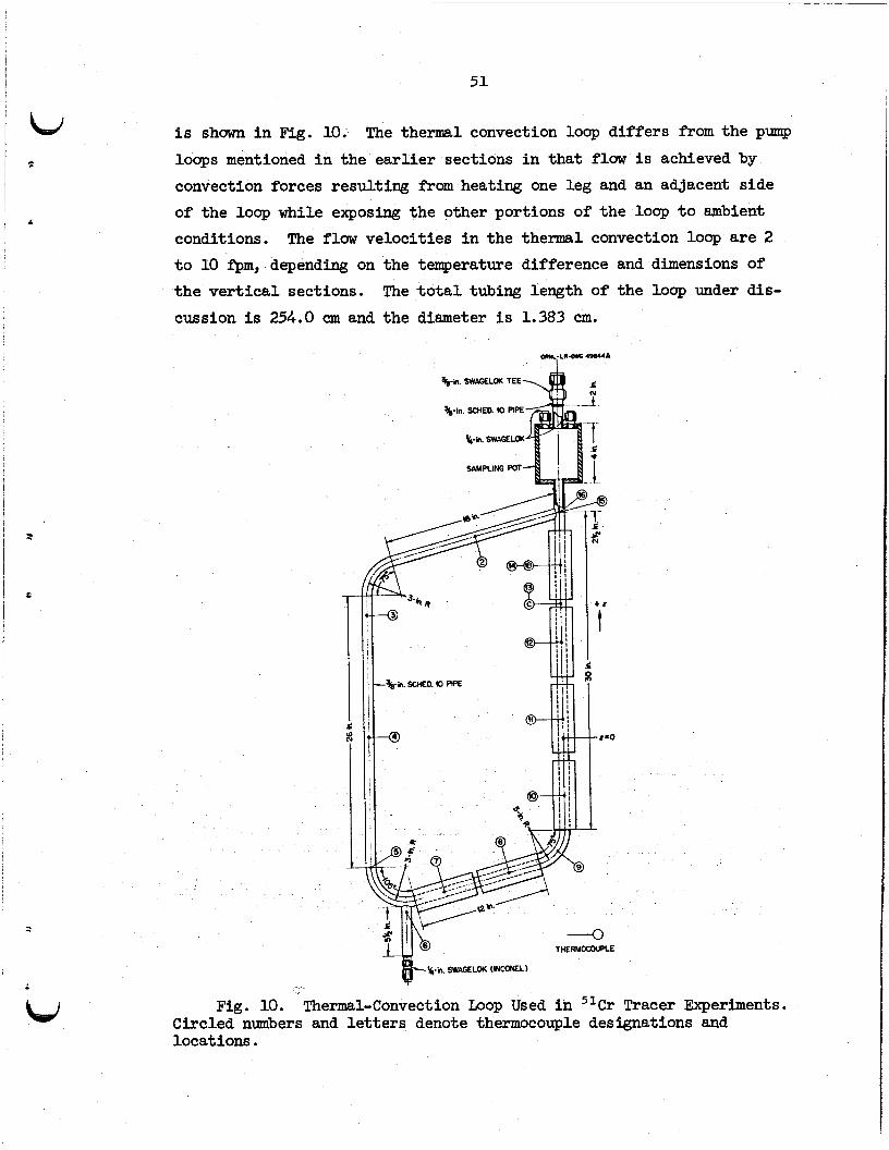
51

is shown in Fig. 10. loops mentioned in the earlier sections in that flow is achieved by convection forces resulting f r o m heating one leg and an adjacent side of the loop while exposing the other portions of the loop to ambient conditions. to 10 f’pm, depending on the temperature difference and dimensions of the vertical sections. cussion is 254.0 cm and the diameter is 1.383 cm.

The thermal convection loop differs f r o m the pump

The flow velocities in the thermal convection loop are 2

The total tubing length of the loop under dis -

Q)*L-LI-D*b 49844p. I

Fig. 10. Thermal-Convection Loop Used in 51Cr Tracer Experiments. Circled numbers and letters denote thermocouple designations and locations.

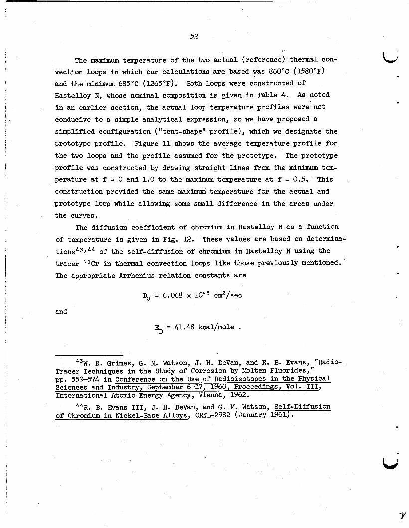
52

,

r

The maximum temperature of the two actual (reference) thermal convection loops i n which our calculations a re based was 860°C (1580°F) and the minimum 685°C (1265°F). Hastelloy N, whose n&al composition i s given i n Table 4 . i n an ear l ier section, the actual loop temperature profiles were not conducive t o a simple analytical expression, so we have proposed a

simplified configuration ( "tent-shape" profile), which we designate the prototype profile. Figure 11 shows the average temperature prof i le for

Both loops were constructed of As noted

the two loops and the prof i le assumed for the prototype. The prototype prof i le was constructed by drawing st raight l ines from the minimum temperature a t f = 0 and 1.0 t o the maximum temperature a t f = 0.5. construction provided the same maximum temperature for the actual and prototype loop while allowing some small difference i n the areas under the curves.

This

The diffusion coefficient of chromium i n Hastelloy N as a ~ c t i o n

of temperature i s given i n Fig. 12. t i o n ~ " , ~ ~ of the self-diffusion of chromium i n Hastelloy N using the tracer 51Cr i n thermal convection loops l i ke those previously mentioned. The appropriate Arrhenius relation constants are

These values are based on determina-

Do = 6.068 x cm2/sec

and

= 41.48 kcal/mole . ED

43W. R. Grimes, G. M. Watson, J. H. DeVan, and R. B. Evans, "Radio- Tracer Techniaues i n the Study of Corrosion by Molten Fluorides," pp. 559-574 ii Conference on the Use of Radioisotopes i n the Physical Sciences and Industry, S e p p , International Atomic Energy Agency, Vienna, 1962. 1

44R. B. Evans 111, J. H. DeVan, and G. M. Watson, Self-Diffusion of Chromium i n Nickel-Base Alloys, ORNL-2982 (January 1961). .

Y

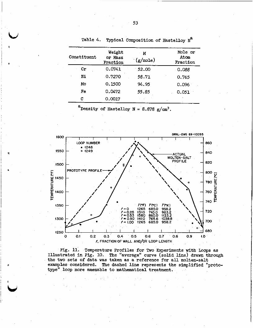
53

Table 4. Typical Composition of Hastelloy N&

' +

Weight M Mole or

Fraction Constituent or Mass At om

Fraction ' (g/mole 1 Cr 0.0741 52.00 0.088 Ni 0.7270 58.71 0.765 Mo 0. I500 94.95 0.096

0.0472 55.85 0.051 Fe C 0.0017

~

a Density of Hastelloy N = 8.878 g/cm3.

ORNL-DWG 6940095 t600 1 I I I I I I I I I I

LOOP NUMBER -4 t 550

1500

0 / 0

(450

/

I \ 4400

0- / 0

1350 r* f = O t265 685.0 958.2 \

0

// f=0.25 fs0 .53 13tO 1580 740.0 860.0 983.2 lf33.2 1300 0 f = 0.90 141 0 765.6 1038.8

f D= t .00 1265 685.0 958.2 1 0

860

840

820

800

780

760

740

720

700

(250 I I I I I I 1 I I I 680 0 0.4 0.2 0.3 0.4 0.5 0.6 0.7 0.8 0.9 t.0

f , FRACTION OF WALL AND/OR LOOP LENGTH

Fig. ll. Temperature Profiles for Two Experiments with Loops as Illustrated in Fig. 10. the two sets of data was taken as a reference for all molten-salt examples considered. type" loop more amenable to mathematical treatment.

The "average" curve (solid line) drawn through

The dashed line represents the simplified "proto-

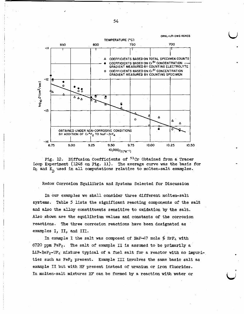
i

I I

/

54

I -11 - I

A COEFFICIENTS BASED ON TOTAL SPECIMEN COUNTS

GRADIENT MEASURED BY COUNTING ELECTROLYTE 0 COEFFICIENTS BASED ON ~ r 5 ' CONCENTRATION -

o COEFFICIENTS BASED ON ~ r 5 ' CONCENTRATION

. . 8.75 9.00 9.25 9.50 9.75 10.00 10.25 (0.50

~O,OOO/T (OK - ' Fig. 12. Diffusion Coefficients of 51Cr Obtained from a Tracer

Loop Experiment (1248 on Fig. 11). DO and 5 used i n a l l computations relat ive t o molten-salt examples.

The average curve was the basis for

Redox Corrosion Equilibria and Systems Selected for Discussion

In our examples we shall consider three different molten-salt systems. and also the alloy constituents sensitive t o oxidation by the salt. Also shown are the equilibrium values and constants of the corrosion reactions. examples I, 11, and 111.

Table 5 lists the significant reacting components of the salt

The three corrosion reactions have been designated as

In example I the salt was composed of NaF-47 mole $ ZrF4 with 6720 ppm FeF2. LiF-BeF2-UF4 mixture typical of a fue l salt for a reactor with no impuri-

t i e s such as FeF2 present. example I1 but with HF present instead of uranium or iron fluorides. In molten-salt mixtures HF can be formed by a reaction with water or

The salt of example I1 i s assumed t o be primarily a

Example I11 involves the same bas ic -sa l t as

LJ

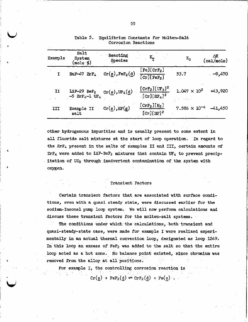
55

Table 5. Equilibrium Constants for Molten-Salt Corrosion Reactions

Reacting Species

S a l t Example System

(mole $1 -

-9,470

111 B q l e 11 Cr(s),m(g) 7.586 X -41,450 [CrF21EH21

salt Ecrl [HFI

other hydrogenous impurities and is u s u a l l y present t o some extent i n a l l fluoride salt mixtures a t the start of loop operation. In regard t o the ZrF4 present i n the salts of examples I1 and 111, certain amounts of

ZrF4 were added t o LiF-BeF2 mixtures that contain UF4 t o prevent precip- i t a t i o n of U@ through inadvertent contamination of the system with

oxygen.

Transient Factors

Certain transient factors that are associated with surface conditions, even w i t h a quasi steady state, w e r e discussed earlier for the

sodium-Inconel pump loop system. We w i l l now perform calculations and discuss these transient factors fo r the molten-salt systems.

The conditions under which the calculations, both transient and quasi-steady-state case, were made for example I were reallzed experimentally in an actual thermal convection loop, designated as loop l249. In th i s loop an excess of FeF2 was added t o the salt so that the ent i re loop acted as a hot zone. No balance point existed, since chromium was

removed fromthe al loy a t a l l positions. For example I, the controlling corrosion reaction i s

C r ( s ) - + FeFz(d) - *'CrF2(d) - + Fe(s) - .

I .

56

On a mass basis Eq. (21b) becomes

where [CrF2] E x

and

are the molecular weights of the respective species; [FeFz] From

?Fey %eF2 and [Fe] are the concentrations, 6720 ppm and 5$, respectively.

Eq. (251,

As i n the l iquid metal case, H was calculated f o r the maximum and m i n i - mum loop temgeratures, -3 and 958°K.

= 4.83 X 10IO/cm . H958 O K = 3.0 X 1OX2/cm .

I$ was calculated f r o m the equation, log K = 1.73 + 2.07 X 103/T, which was obtained f r o m combining experimental equilibrium quotients of the react ions 45

CrF&) + H2(g) FfCr(s) - + 2 HF(g)

i

45C. M. Blood e t al., Reactor Chem. Div. Ann. Progr. Rept. Jan. 31, -, 1960 ORNL-2931, pp. 39-43.

57

i n NaFA7 mole $ ZrF4. We used pQ(salt) = 3.71 - 8.90 X l W 4 T('C) = 2.945 g/cm3 at 1133"Ky pa f'rom Table 4, and D f r o m Fig. 12.

The l iquid film coefficient, h, i s obtained from a combination of dimensionless groups, and we have calculated it for both turbulent and laminar f law.

NRe = m/cI, Nsc = p/pD, and d = 1.383 cm. For turbulent flow, Nsh = 0.023NRe0'8Nsc0*33, where Nsh = dh/D,

1.383h 1.383(1.422) (2.945) ]"*8L 2.62 X lo'* = 0.023[

4.166 X loo5 2.62 X loo2 .945(4.166 X loo5)

or h = 3.065 x t a l values46:

The viscosity, py was extrapolated f'rom experimen-

T, "C 600 700 800 p, centipoise 7.5 4.6 3.2

The l iquid diffusion coefficient is calculated f r o m the Stokes- Einstein equation, where

1.38 x 10-16(1133) %r(d)-salte - 1 1 1 3 3 ° K =

2.62 X 10-2(6)(3.U2)(0.76 X lo-') = 4.17 x cm2/sec

and the velocity of the s a l t = 2,8 f'pm = 1.422 cm/sec i s taken from t h

loop operating conditions. There i s always the question of whether the f l a w i n a thermal con-

vection loop i s laminar or turbulent. mass transfer equation can be written and h can be calculated. value is suff ic ient ly close t o the h calculated with the equation f o r turbulent f l aw so that the former h w i l l be used i n subsequent calculations.

For the case of Laminar flowy a Its

4 6 ~ . Cantor, ORNL, personal communication.

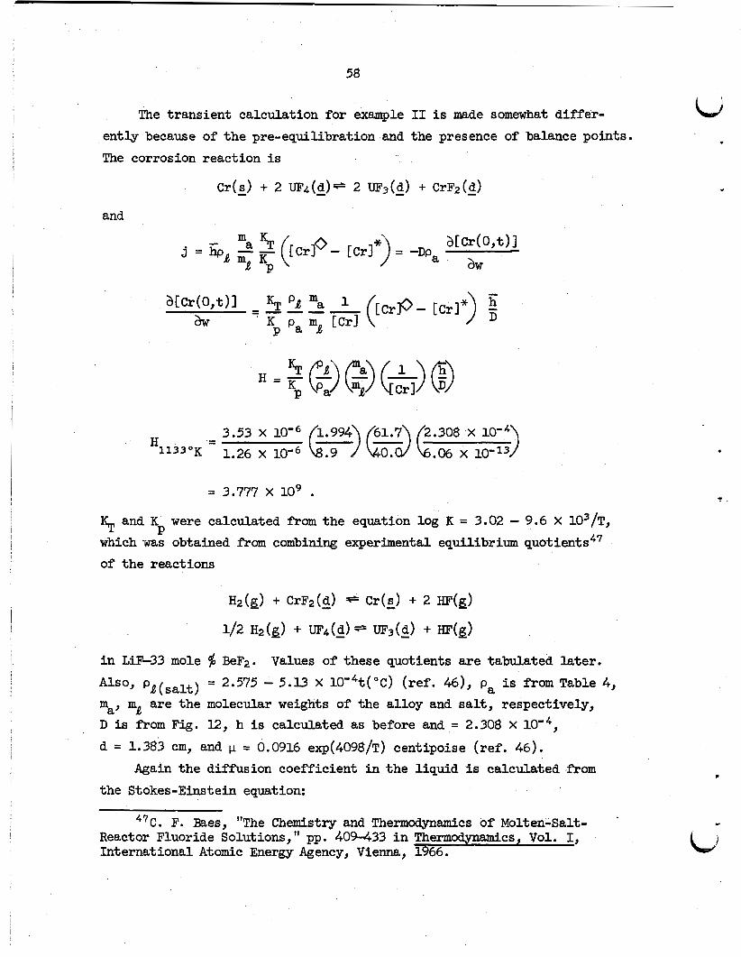
58

The transient calculation for example I1 i s made somewhat differ- LJ ently because of the pre-equilibration and the presence of balance points. The corrosion reaction is

. Cr(s) + 2 UF4(d)== - 2 UF3(g) + CrFa(d) -

and

% H = - P K

% and K were calculated from the equation log K = 3.02 - 9.6 X 103/T, P

which -was obtained from combining experimental equilibrium quotients47 of the reactions

i n LiF-33 mole

P a ( s a l t ) m m a re the D is f'rom Fig. a' a

BeF2. 2.575 - 5.13 X 10'4t(0C) ( re f . 46), pa i s from Table 4,

Values of these quotients a re tabulated la te r .

molecular weights of the alloy and salt, respectively, 12, h is calculated as before and = 2.308 X

d = 1.383 cm, and = 0.0916 eq(4098/T) centipoise ( re f . 46). Again the diffusion coefficient i n the l iquid is calculated from

the Stokes -Eins t ein equation:

47C. F. Baes, "The Chemistry and Thermodynamics of Molten-Salt- Reactor Fluoride Solutions," pp. 409433 i n Thermodynami cs, VOl. I, International Atomic Energy Agency, Vienna, 1966.

+

t .

c

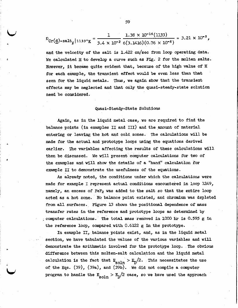
59

and the velocity of the salt is 1.422 cm/sec from loop operating data. We calculated H t o develop a curve such as Fig. 2 for the molten sa l t s . However, it became quite evident that , because of the high value of H

for each example, the transient effect would be even less than that seen for the l iquid metals. Thus, we again shuw that the transient effects may be neglected and tha t only the quasi-steady-state solution need be considered.

Quas i-St eady- Stat e Solutions

Again, as i n the l iquid metal case, we are required t o find the balance points ( i n examples I1 and 111) and the amount of material entering or leaving the hot and cold zones. made fo r the actual and prototype loops using the equations derived

The calculations w i l l be

ear l ier . then be discussed. the examples and w i l l shuw the de ta i l s of a "hand" calculation for example I1 t o demonstrate the useflilness of the equations.

made fo r example I represent actual conditions encountered i n loop l%9, namely, an excess of FeF2 was added t o the s a l t so tha t the ent i re loop acted as a hot zone. from all surfaces. t ransfer ra tes i n the reference and prototype loops as determined by

The variables affecting the resul ts of these calculations w i l l We w i l l present computer calculations for two of

As already noted, the conditions under which the calculations were

No balance point existed, and chrumium was depleted Figure l3 shows the posit ional dependence of mass

~ computer calculations. The t o t a l mass removed i n 1000 hr is 0.595 g i n the reference loop, compared w i t h 0.6122 g i n the prototype.

section, we have tabulated the values of the various variables and w i l l demonstrate the arithmetic involved for the prototype loop. difference between this molten-salt calculation and the l iquid metal calculation i s the fac t that Esoh > 5 / 2 .

of the Eqs. (391, (39a), and (39b). program t o handle the Esoh > %/2 case, so we have used the approach .

In example 11, balance points exist, and, as i n the l iquid metal

The obvious

This necessitates t h e use

We did not compile a computer

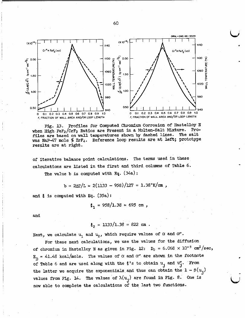
60

- I I I I I I I I I - 1140

- W

0 0.i 0.2 0.3 0.4 0.5 0.6 0.7 0.8 0.9 1.0 f. FRACTION OF WALL AREA AND/OR LOOP LENGTH

ORNL-DWG 69-9929

- - ((40

W E 3

0 0.1 0.2 0.3 0.4 0.5 0.6 0.7 0.8 0.9 1.0 f , FRACTION OF WALL AREA AND/OR LOOP LENGTH

Fig. 13. Profiles for Computed Chromium Corrosion of HasteUoy N Pro-

Reference loop resul ts a re a t left;; prototype

when High) FeF2/CrF2 Ratios a re Present i n a Molten-Salt Mixture. f i l es a re based on wall temperatures s h m by dashed l ines. was NaF47 mole resul ts are at right.

The s a l t ZrF4.

of i t e ra t ive balance point calculations. calculations are l i s t ed i n the first and th i rd columns of Table 6.

The terms used i n these

The value b i s computed with Eq. (34a) :

b = m / L = 2(l l33 - 958)/127 = 1.38"K/~m , and is computed with Eq. (35a) :

E, = 958/1.38 = 695 cm , and

E, = 1133/1.38 = 822 . Next, we calculate u1 and u2, which require values of a and a".

of chromium i n Hastelloy N as given in Fig. 12:

ED = 41.48 kcal/mole. of Table 6 and are used along with the E's t o obtain u and ut!. the l a t t e r we acquire the exponentials and thus can obtain the 1 - f3(uj) values from Fig. U. now able t o complete the calculations of the last two functions.

For these next calculations, we use the values fo r the diffusion Do = 6.068 X cm2/sec,

The values of a! and a!" are shown i n the footnote From 5 J

The values of A(u ) are found in Fig. 8. One i s j

bi

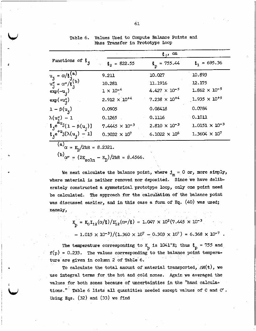
61

1

i

. : w

Table 6. Values Used t o Compute Balance Points and Mass Transfer i n Prototype Loop

tap ep = 755.44 5, = 695.36 3 e, = 822.55

Functions of 5

~~~

uj = d e j (a) 9 .2 l l 10.027 10.893

u'! = att/g (b) 10.281 11.1916 12.175

exp (-u4 1 1 x 101~ 4.427 X 1.862 X 3

J

exp ( +ut1 ) 3 2.912 x 7.238 x ,1.935 x 10+5

1 - B(Uj) 0.0905 0.08418 0.0784

A(u!!) - 1 0.1265 0.1ll6 0. l o l l

We next calculate the balance point, where jm = 0 or, more simply, where material is neither removed nor deposited. erately constructed a symmetrical prototype loop, only one point need be calculated. The approach for the calculation of the balance point was discussed earlier, and i n t h i s case a form of EQ. (40) was used;

n?,melY,

Since we have delib-

K = $112(QI/S)/I~2(CV~/S) = 1.047 X lO'(7.445 X P

- 1 . O Z X 10-3)/(l.360 X lo7 - 0,303 x lo7) = 6.368 X . The temperature corresponding t o K i s lW1"K; thus 5 = 755 and

The values corresponding t o the balance point tempera-

To calculate the t o t a l amount of material transported, AM(%), we

Again we averaged the

P P f (p ) = 0.233. ture a re given i n column 2 of Table' 6.

use integral t e r m for the hot and cold zones. values for both zones because of uncertainties i n the "hand calculations."

Using Eqs. (32) and (33) we find

Table 6 l ists a l l quantities needed except values of C and C'.

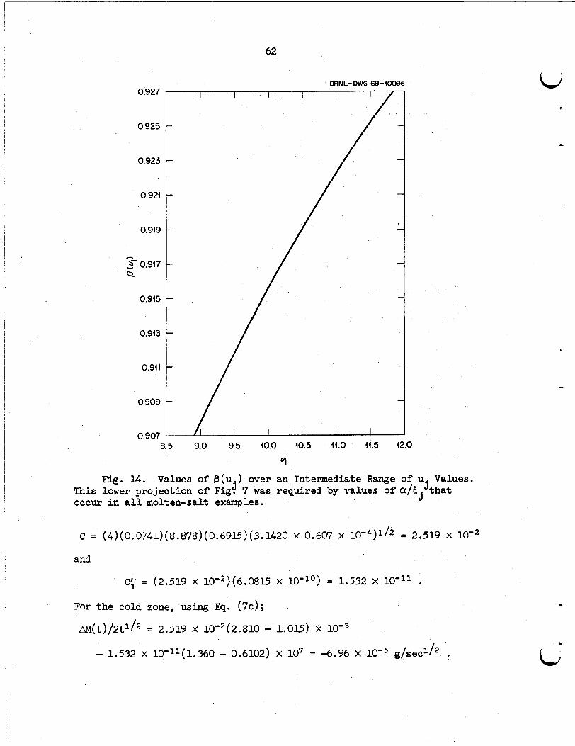
62

0.927

0.925

0.923

0.924

0.949

- 2- 0.947 Q

0.945

0.943

0.944

0.909

0.907

ORNL- DWG 69-40096

8.5 9.0 9.5 40.0 40.5 44.0 41.5 42.0

*j

Fig. Ut. Values of @(u ) over an Intermediate Range of u Values.

3 j j This lower projection of Fig. 7 was required by values of a/[. that

occur in all molten-salt examples.

C = (4)(0.0741)(8.878)(0.6915)(3.U20 X 0.607 X 10-4)1/2 = 2.519 X

and

C; = (2.519 x 10'2)(6.0815 x 10-l') = 1.532 X . For the cold zone, using Eq. ( 7 ~ ) ;

AM(t)/2t1I2 = 2.519 X 10'2(2.810 - 1.015) X lom3

- 1.532 X 10'11(1.360 - 0.6102) X lo7 = -6.96 x g/sec1/2 .

L)

r

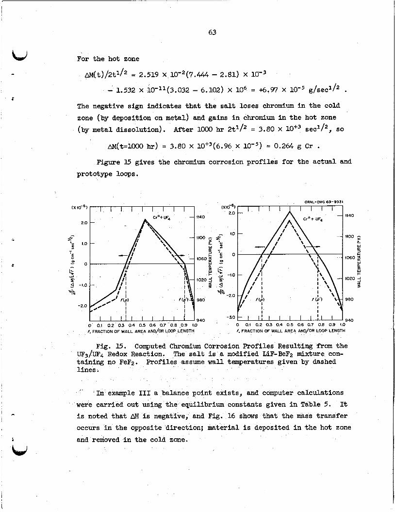
63

For the hot zone

~lM(t)/2t’/~ = 2.519 X 10‘2(7.444 - 2.81) X low3 - 1.532 X 10’11(3.032 - 6.102) X lo6 = 6.97 X low5 g/sec1/2 .

The negative sign indicates tha t the salt loses chromium i n the cold zone (by deposition on metal) and gains i n chromium i n the hot zone (by metal dissolution). After 1000 hr 2t1/2 = 3.80 X sec1/2, so

AM(t=1000 hr) = 3.80 X 10+3(6.96 x = 0,264 g C r ,

Figure 15 gives the chromium corrosion prof i les for the actual and prototype loops.

2.0 -

- 1100 G -

W P 3 t

W to60

a

P to20 =I s 980

I I I I I I I I I 1 1 t 940

0 0.1 0.2 0.3 0.4 0.5 0.6 07 0.8 0.9 4.0 t. FRACTION OF WALL AREA AND/OR LOOP LENGTH

ORNL-DWG 69-9931

tl40

t400 - w P 3

I060 W a

I- 5

I020 d a 3

980

I I I I I I I I l l I I I -30 940

0 0.t 0.2 0.3 0.4 0.5 0.6 0.7 0.8 0.9 4.0 f. FRACTION OF WALL AREA AND/OR LOOP LENGTH

Fig. 15. Computed Chromium Corrosion Profiles Resulting from the UF~/UFI, Redox Reaction. taining no FeF2. l ines.

The salt i s a modified LIF-BeF2 mixture con- Profiles assume w a l l temperatures given by dashed

’ In example I11 a balance point exists, and computer calculations ’ were carried out using the equilibrium constants given in Table 5. It

i s noted tha t AH i s negative, and Fig. 16 shows tha t the mass t ransfer occurs i n the opposite direction; material i s deposited i n the hot zone and renioved i n the cold zone.

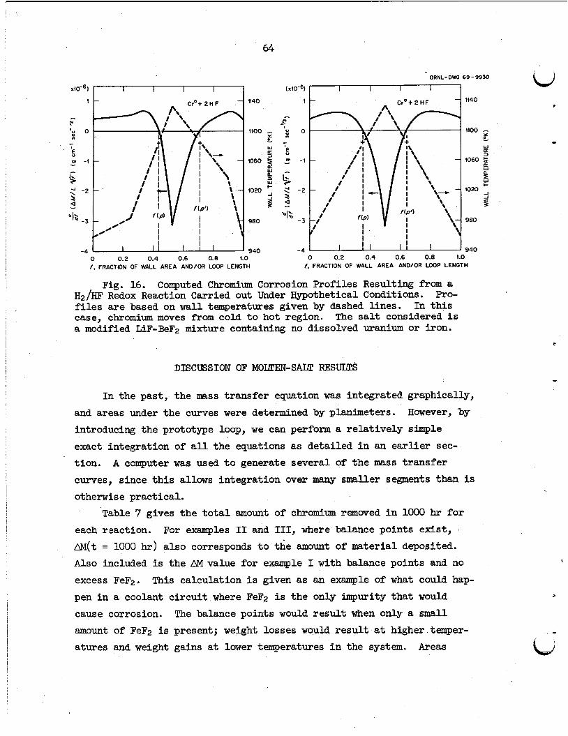
64

I I I

1140

1100

1060

1020

980

ORNL- DWG 69 - 9930 (x10-6) 9 1

1140

4100

1060

1020

980

940

- K a t a a J

I

- W

3

W

I-

J J

_ _ 0 0.2 0.4 0.6 0.8 1.0 0 0.2 0.4 0.6 0.8 1 .o

Fig. 16. Computed Chromium Corrosion Profiles Resulting from a H2.m Redox Reaction Carried out Under Hypothetical Conditions. f i les are based on w a l l temperatures given by dashed lines. In t h i s case, chromium moves fYom cold t o hot region. a modified LiF-BeFz mixture containing no dissolved uranium or iron.

f , FRACTION OF WALL AREA AND/OR LOOP LENGTH f , FRACTION OF WALL AREA AND/OR LOOP LENGTH

Pro-

The salt considered i s

DISCUSSION OF MOLTEN-SALT RESULTS

In the past, the mss transfer equation was integrated graphically, However, by and areas under the curves were determined by planimeters.

introducing the prototype loop, we can perform a relat ively slmple exact integration of a l l the equations as detailed i n an earlier section. curves, since t h i s allows integration over many smaller segments than is otherwise practical.

A computer was used t o generate several of the mass transfer

T,Etble 7 gives the t o t a l amount of chromium remuved i n 1000 hr for each reaction. AM(t = 1000 hr) a lso corresponds t o the amount of material deposited. A l s o included i s the AMvalue for example I with balance points and no excess FeF2. pen i n a coolant c i rcui t where FeF2 i s the only impurity tha t would cause corrosion. The balance points would resul t when only a small amount of FeF2 is present; weight losses would resu l t a t higher temperatures and weight gains at luwer temperatures i n the system.

For examples I1 and 111, where balance points exist,

This calculation i s given as an example of what could hap-

Areas

li I

*

_.

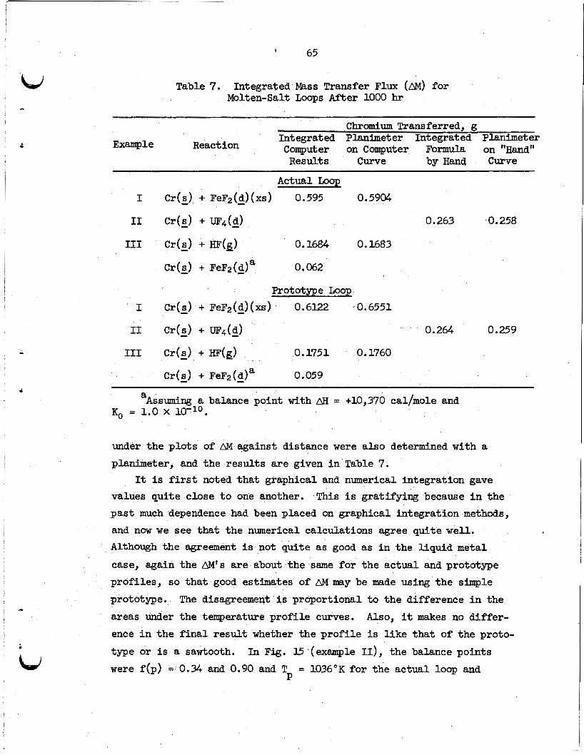
1 65

t

C h r o m i u m Transferred, g Integrated Planimeter Integrated Planimeter

React ion Computer on Computer Formula on "Hand" Example Results Curve by Hand Curve

Table 7. Integrated Mass Transfer Flux (AM) for Molten-Salt Loops After 1000 hr

. U

I

I1

I11

I

I1

I11

Actual Loop Cr(s) + FeFz(d)(xs) - 0.595 0.5904 - C r ( s ) + UFb(d) - Cr(s) + H F ( ~ ) 0.1684 0.1683

Cr(s) - + FeF2(d)' c 0.062

Prototype Loop Cr(s) - + FeFn(d)(xs) - 0.6122 ~0.6551

Cr(g> + 0.1751 0.1760

C r ( s ) - + FeF2(dla - 0.059

0.263

0.264

0.258

0.259

a Assuming a balance point with AH = +10,370 cal/mole and KO = 1.0 X low1'.

under the plots of AM wa ins t distance were also determined with a

planimeter, and the results are given i n Table 7.

values quite close t o one another. past much dependence had been placed on graphical integration methods, and now we see that the numerical calculations agree quite w e l l . Although the agreement i s not quite as good as i n the l iquid metal

case, again the AM's are about the same fo r the actual and prototype profiles, so tha t good estimates of AM may be made using the s h p l e

prototype. areas under the temperature prof i le curves. ence i n the f i n a l resu l t whether the prof i le is l i ke tha t of the proto-

type or is a sawtooth. were f(p) = 0.U. and 0.90 and T

It i s first noted that graphical and numerical integration gave This i s gratifying because i n the

The disagreement is proportional t o the difference i n the

Also, it makes no differ-

In Fig. I5 (example 11), the balance points = 1036°K f o r the actual loop and

P

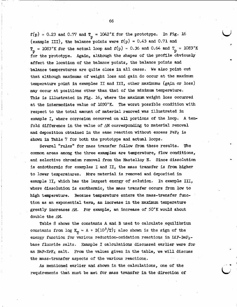
66

f (p) = 0.23 and 0.77 and T

(example 111), the balance points were f(p) = 0.43 and 0.71 and

= 1042°K for the prototype. In Fig. 16 P

= 1083°K for the actual loop and f(p) = 0.36 and 0.64 and T = 1083°K TP P for the prototype. affect the location of the balance points, the balance points and balance temperatures are quite close i n a l l cases. tha t although maximums of weight loss and gain do occur a t the maximum temperature point i n examples I1 and 111, other maximums (ga;in or loss) may occur a t positions other than tha t of the minimum temperature. This i s i l lus t ra ted i n Fig. 16, where the maximum weight loss occurred at the intermediate value of 1030°K. respect t o the t o t a l amount of material removed was i l lus t ra ted i n example I, where corrosion occurred on a l l portions of the loop.

fold difference i n the value of AM corresponding t o material removal and deposition obtained i n the same reaction without excess FeFz i s

shown i n Table 7 for both the prototype and actual loops.

Again, although the shapes of the prof i le obviously

We also point out

The worst possible condition with

A ten-

Several "rules" for mass transfer follow from these results. The common areas among the three examples are temperature, f low conditions, and selective chromium removal from the Hastelloy N. Since dissolution i s endothermic for examples I and 11, the mass transfer i s from higher t o lower temperatures. example 11, which has the largest energy of solution.

where dissolution i s exothermic, the mass transfer occurs from low t o high temperature. Because temperature enters the mass-transfer func- t i on as an exponential term, an increase i n the maximum temperature greatly increases AM. For example, an increase of 50°K would about double the AM.

More material i s removed and deposited i n In example 111,

Table 8 shows the constants A and B used t o calculate equilibrium constants from log energy function for various reduction-oxidation reactions i n LTF-BeF2- base fluoride salts.

an NaF-ZrF4 salt. the mass-transfer aspects of the various reactions.

= A + B(103/T); also shown i s the sign of the I(r

Example I calculations discussed ear l ier were for From the values given i n the table, we w i l l discuss

As mentioned ear l ier and shown i n the calculations, one of the requirements that must be met for mass transfer i n the direction of

L, ,

i

LJ

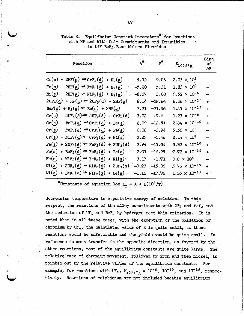
67

Table 8. Equilibrium Constant Parameters' for Reactions with HF and With Salt Constituents and Impurities

in LiF- BeF2 - Bas e Molt en Fluorides

React ion Sign

m Aa Ba K3075°K of

2.03 X 103 1.83 X 10' 9.52 X

6.06 X loo1' 1.43 x 10-13 1.23 X

2.84 X 10-l'

5.56 x 103 2.u x 108

7.77 x 10-l4

5.76 x 10-15

3.32 X 10-l'

8.8 X lo4

1.35 X

a Constants of equation log 5 = A + B(~o~/T).

decreasing temperature is a positive energy of solution.

respect, the reactions of the alloy constituents with UF4 and BeF2 and the reduction of UF4 and BeF2 by hydrogen meet this criterion. It is noted that in all these cases, with the exception of the oxidation of chromium by UF4, the calculated value of K is quite small, so these reactions would be unfavorable and the yields would be quite small. In reference to mass transfer in the opposite direction, as favored by the other reactions, most of the equilibrium constants are quite large. The relative ease of chromium movement, followed by iron and then nickel, is pointed out by the relative values of the equilibrium constants. example, for reactions with UF4, K107,0K = and respectively.

In this

For

Reactions of molybdenum are not included because equilibrium

68

constants are not available.

formation of molybdenum and nickel fluorides are nearly equal, we would expect the equilibrium constants t o be about the same.

considered t o measure the U(III)/U(Iv) r a t i o and thus determine the oxidizing or reducing potential of the UF4-containing molten salt. Additions of beryllium are being used t o adjust th i s potential and con- t r o l the corrosion rate. possible application of 95Nb deposition as the redox indicator. 48

However, because the free energies of

With respect t o the UF4 corrosion reaction, methods are now being

Investigations are a lso under way for the

We also wish t o consider i f loop conditions are actually the same as those under which the equilibrium quotients were determined. we beg the question: of luw t o high temperature as is theoretically shown from the FeF2 and HF reactions with balance points i n LiF-BeF2 salts? work4’ i n salt systems containing UF4, FeF2, and €€I? show evidence of

mass transfer only from high t o l c r w temperature. knuwn about the effects of the canbinations of the reactants or what

Actually

can mass transfer occur i n a loop i n the direction

Recent experimental

However, nothing is

effect removal of elements other than chromium from the al loy m i g h t have on the overall process. It would be interesting t o speculate what r a t i o of CrF2 t o FeF2 would be needed i n a UF4-containing salt t o stop the mass-transfer (and the corrosion) process altogether. goal w m l d be t o carefully isolate the above components and t o run the verifying experimental tests i n loops.

A promising future

I n salts proposed for use i n a breeder reactor systen, ThF4 i s includLed. affect the corrosion process.

The ThF4 w i l l not oxidize chromium, so i t s presence w i l l not

It must be again emphasized that there is a paral le lbetwem the

resul ts i n Report I and here. were derived as analogs of heat f low equations. type consist of driving forces and resistances. Report I were based on the first-order reaction r a t e constant and the

The mass-transfer equations of Report I

Rate equations of t h i s

The resistances i n /

4J f

48R. E. Thoma, ORNL, personal communication. 49J. W. Koger and A. P. Litman, MSR Program Semiann. Progr. Rept.

Feb. 28, 1969, 0-4396, pp. 243-253. Lid

69

L J f i l m coefficient. i n both mechanisms. the important difference is that between the equilibrium corrosion product solute concentrations at the high and low temperatures of the system, while, when diffusion controls, the difference i s that between

The driving forces are differences that are involved For example, when solution rate is controlling,

the bulk alloy concentration and the surface alloy concentration of the

active alloying element. The results do not depend on the shape of the prof i le i n the mechanism of Report I and only sometimes i n the mechanism given here. ture (position) i n Report I, while here we assume constant concentration of the corrosion product throughout the loop. because the use of the equilibrium constant allows us t o change only one

variable with temperature.

The corrosion product concentration differed with tempera-

This i s quite important,

This was not possible i n Report I.

As we mentioned earlier, liquid velocities i n pump loops are

orders of magnitude greater than those i n thermal convection loops. Throughout th i s report we have assumed that conclusions about pump loop corrosion behavior are good for thermal convection loops and vice versa.

O f course, i f the process is t ru ly controlled by solid-sta6e diffusion i n the alloy, then velocity w i l l not affect the mass transfer.

SUMMARY

We have elected t o summarize the molten-salt resul ts since we wish t o illustrate several cogent points. In t h i s portion of the report our

main purpose was t o discuss the molten-salt corrosion (mass transfer of

chromium) of Hastelloy N i n polythermal loops for cases where solid- s t a t e diffusion controls throughout the system. the versa t i l i ty of the method by showing three different examples: removal of chromium from a l l portions of the loop, hot-to-cold leg transfer, and cold-to-hot leg transfer.

We have demonstrated

Calculations for both transient and quasi-steady-state conditions were based on a mathematical development of the idealized diffusion process, wherein corrosion rates depend direct ly on the r a t e a t which

b constituents of alloys diffuse into, or out of, container walls as influ-

W enced by the condition of w a l l surfaces exposed t o a high-temperature

70

liquid. The transient effects (the effects of mass transfer across the

l iquid films on corrosion) w e r e negligible because of t he i r short dura-

t ion. The quasi-steady-state condition assumed a pre-equilibration of

the salt w i t h CrF2 such that the concentration of CrF2 did not change. The balance points and the amount of material entering or leaving

the various zones of the loops fo r the various systems were determined for the quasi steady state. prototype "tent-shaped" and actual loop temperature profiles. resul ts obtained from the prototype, which were qQite simple t o calculate, agreed very well with the resul ts from the actual profile. t an t variables discussed i n th i s treatment w i t h respect t o the mass transfer process were the energy of solution of the corrosion reaction, the energy of activation for diffusion, the equilibrium constant of the corrosion reaction, and i t s temperature dependence.

The calculation was adaptable fo r both the The

Impor-

I n conclusion, the practical importance of the calculations lies i n the fac t that, i f the proper experimental data are available, one may determine, before running a loop test, the magnitude and manner i n which the mass transfer w i l l occur. expected i n a completed experiment i f the temperature conditions are varied w i t h the developed equations. i s the fact that a p r io r i calculations of t h i s type are required t o

predict the concentration tha t w i l l give a pre-equilibration condition a t the beginning of an experiment. This i s necessary for one t o run a systematic well-developed test.

One may also predict the changes

O f perhaps even greater importance

,

V i

.

- -

Lid

I

I

hd

E

71

0-4575, Volume 2

INTERNAL DISTRIBUTION

1-3. Central Research Library 4. ORNL Y-12 Technical Library

Document Reference Section 5-24. Laboratory Records

25. Laboratory Records, ORNL RC 26. ORNL Patent Office 27. G. M. Adamson, Jr. 28. J. L. Anderson 29. R. F. Apple 30. D. E. Arnurius 31. W. E. Atkinson 32. C. F. Baes 33. C. E. Bamberger 34. C. J. Barton 35. H. F. Bauman 36. S. E. Beall 37. M. J. Bell 38. C. E. Bettis 39. D. S. Billington 40. R. E. Blanco 41. F. F. Blankenship 42. R. Blumberg 43. E. G. Bohlmann 4.4. G. E. Boyd 45. J. Braunstein 46. M. A. Bredig 47. R. B. Briggs ,

48. H. R. Bronstein 49. G. D. Brunton 50. S. Cantor 51. D. W. Cardwell 52. H. P. Carter 53. W. L. C a r t e r 54. 0. B. Cavin 55. Nancy Cole 56. C. W. Collins 57. E. L. Compere 58. W. H. Cook 59. J. W. Cooke 60. L. T. Corbin 61. J. L. Crawley 62. F. L. Culler, Jr. 63. D. R. Cuneo 64. J. E. Cunningham 65. J. M. Dale 66. H. J. de Nordwall

___

67-69. 70. 71. 72. 73.

74-78. 79. 80. 81. 82. 83. 84. 85. 86. 87. 88. 89. 90. 91. 92. 93. 94. 95. 96. 97. 98. 99 *

100-102. 103. 104. 105. 106. 107. 108.

. 109. 110. 111. 112. 113. 1%. u5. 116.

117-121. u2. 123. 3.24.

J. H. DeVan J. R. DiStefano S. J. Ditto W. P. Eatherly J. R. Engel R. B. Evans I11 J. I. Federer M. Feliciano D. E. Ferguson B. Fleischer M. Fontana A. P. Fraas J. H Dye, Jr. W. K. Furlong C. H. Gabbard D. A. Gardiner R. E. Gehlbach L. 0. Gilpatrick G. Goldberg W. R. Grimes A. G. Grindell R. H. Guymon W. 0. H a m P. N. Haubenreich R. E. Helms R. F. Hibbs J. R. Hightower M. R. H i l l E. C. H i s e H. W. Hoffman D. K. Holmes P. P. Holz W. R. Huntley J. E. Inman H. Inouye W. H. Jordan P. R. Kasten R. J. Ked1 C. R. Kennedy J. J. Keyes, Jr. S. S. Kirslis R. L. Klueh J. W. Koger H. W. Kohn R. B. Korsmeyer A. I. Krakoviak

72

125. 126. 127. 128. 129. 130. 131. 132. 133. l34. 135. 136. 137. 138. 139. *

u0 . 141. u.2. u3. 14.4. 145. 246. u7. 148. u 9 . 150. 151. 152. 153. 154. 155. l56. 157. 158. l59. 160. 161. 162. 163. 164. 165. 166. 167.

T. S. mess J. A. Lane R. B. Lindauer D. B. Lloyd E. L. Long, Jr. M. I. Lundin R. N. Lyon R. E. MacPherson A. P. Malinauskas D. L. Manning W. R. Martin H. E. McCoy D. L. McElroy C . K. McGlothlan C . J. McHargue H. A. McLain B. McNabb L. E. McNeese J. R. McWherter A. S. Meyer A. J. Miller R. L. Moore D. M. Moulton T. R. Mueller Paul Nelson, Jr. C. W. Nestor, Jr. H. H. Nichol J. P. Nichols E. L. Nicholson T. S. Noggle L. C. Oakes 0. S. Oen S. M. O h r R. B. Parker P. Patriarca R. B. Perez A. M. Perry T. W. Pickel H. B. Piper C. B. Pollock B. E. Prince G. L. Ragan D. M. Richardson

168. R. C. Robertson 169. K. A. Romberger 170. M. W. Rosenthal 171. G. Samuels 172. H. C. Savage 173. W. F. Schaffer 174. Dunlap Scott 175. 3. L. Scott 176. J. H. Shaffer 177. W. H. Sides 178. V. A. Singletary 179. G. M. Slaughter 180. A. N. Smith 181. F. J. Smith 182. G. P. Smith 183. 0. L. Smith 184. I. Spiewak 185. R. A. Strehlow 186. J. R. Tallackson 187. R. E. Thoma 188. M. L. Tobias 189. D. B. Trauger 190. W. E. Unger 191. G. M. Watson 192. J. S. Watson 193. H. L. Watts 194. C. F. Weaver 195. A. M. Weinberg 196. J. R. Weir 197. M. E. Whatley 198. J. C . White 199. R. P. Wichner 200- L. V. Wilson 201. Gale Young 202- H. C. YOW 203. J. P. Young 204. E. L. Youngblood 205. F. C . Zapp 206. 2W. Leo Brewer (consultant) 208. Jan Korringa (Consultant) 209. Sidney Siege1 (Consultant)

C. M. Adms, Jr. (Consultant)

EXTERNAL DISTRIBUTION

210. R. E. Anderson, SNS, AEC, Washington, DC 20545 211. W. Brehm, WADCO, P. 0. Box 1970, Richland, WA 99352

212-213. E. G. Case, Division of Reactor Standards, RDT, AEC, Washington, DC 20545

L 4 5

.

!

73

...

LJ

214. 215. 216. 217.

218.

219. 220.

221. 222.

223.

224. 225.

226. 227.

228. 229. 230. 231. 232.

233. 234-235,

236.

237-239.

240.

241. 242.

243.

244. 245. 246. 247.

248. 249.

250. 251. 252.

R . L. koats, Sandia Corp., P. 0. Box 5800 Albuquerque, NM 87115 K. P. Cohen, General Electric, BRDO, Sunnyvale, CA 94086 D. F. Cope, RDT, SSR, AEC, Oak Ridge National Laboratory D. R. deBoisblanc, Ebasco Service, Inc., 2 Rector St.,

C. B. Deering, EUack and Veatch, P. 0. Box 8405,

A. R. DeGrazia, RDT, AEC, Washington, DC 20545 L. F. Epstein, LMFBR Program Office, Argonne National Laboratory,

J. E. Fox, RDT, AEC, Washington, DC 20545 K. Goldman, United Nuclear Corp., Grasslands Rd.,

D. H. Gurinsky, -Brookhaven National Laboratory, Upton, Long

Norton Haberman, RDT, AEC, Washington, DC E. E. Hoffbn, General Electric, Nuclear Systems Program,

K. E. Horton, RDT, AEC, Washington, DC 20545 T. F. Kassner, Argonne National Laboratory, 9700 South Cass

E. C. Kovacic, RDT, AEC, Washington, DC 20545 Kermit Laughon, RDT, CSR, AEC, Oak Ridge National Laboratory A. P. Litman, SNS, AEC, Washington, DC 20545 G. Long, UKAEA, Harwell, England H. G. MacPherson, Nuclear Engineering Department, University

C. L. Matthews, RDT, CSR, AEC, Oak Ridge National Laboratory T. W. McIntosh, RDT, AEC, Washington, DC 20545 J. M. McKee, Argonne National Laboratory, 9700 South Cass Ave.,

P. A. Morris, Division of Reactor Licensing, FDT, AEC,

P. Murray, Westinghouse, ARD, Waltz M i l l Site, P. 0. Box 158,

J. Neff, RDT, AEC, Washington, DC 20545 H. Pearlman, Atomics International, P. 0. Box 309, Canoga Park,

T. K. Roche, S te l l i t e Division Cabot Corp., 1020 W. Park Ave.,

H. M. Roth, AEC, Oak R i d g e Operations D. W. Shannon, WADCO, P. 0. Box 1970, Richland, WA 99352 M. Shaw, RDT, AEC, Washington, DC 20545 A. A. Shoudy, Atomic Power Development Associates, Inc.,

J. M. Simons, FDT, AEC, Washington, DC 20545 E. M. Simons, Battelle Memorial Insti tute, 505 King Ave.,

3. Singer, RDT, AEC, Washington, DC 20545 W. L. Smalley, AEC, Oak Ridge Operations E a r l 0. Smith, Black and Veatch, P. 0. Box 8405, Kansas

New York, NY 10006

Kansas City, MO 64lU

9700 South Cass Ave., Argonne, I L 60439

Elmsford, NY 10523

Island, NY 11973 20545

P. 0. Box 15132, Cincinnati, OH 45215

Ave., Argonne, I L 6N39

of Tennessee, Knoxville. TN 37916

Argonne, I L 60439

Washington, DC 20545

Madison, PA 15663

CA 91305

Kokomo, I N 46901

1911 F i r s t Street, Detroit, M I 48226

Colunibus, OH 43201

City, MO 64lU

74

253. J. A. Swartout, Union Carbide Corp., 270 Park Ave., New York, NY

254. A. Taboada, RDT, A E C , Washington, DC 20545 255. C. Tyzack, UKAEA, Culcheth, England 256.

257.

258. 259. Patent Office, AEC, Oak Ridge Operations

10017

J. R. Weeks, Brookhaven National Laboratory, Upton, Long Island,

G. A. Whitlaw, Westinghouse, ARD, Waltz Mill Si te , P. 0. Box 158,

Iaboratory and University Division, AFC, Oak Ridge Operations

NY 11973

Madison, PA 15663

26C-454. Given distribution as shown i n TID-4500 under Metals, Ceramics and Materials category (25 copies - NTIS)

c

c

Documents

Corrosion in Polythermal Loop Systems II. A Solid-State ...moltensalt.org/references/static/downloads/pdf/ORNL-4575.pdf'0 - p ornl4575, volume 2 contract no. w-7405-eng-26 metau and