\images\166_Cover.jpg

Appendices to include in PDF:1 Pavement Conditions yes2 Traffic Performance yes3 Annual Average Daily yes3 Ramp Details no4 Traffic Methodology yes5 Glossary and Referen yes

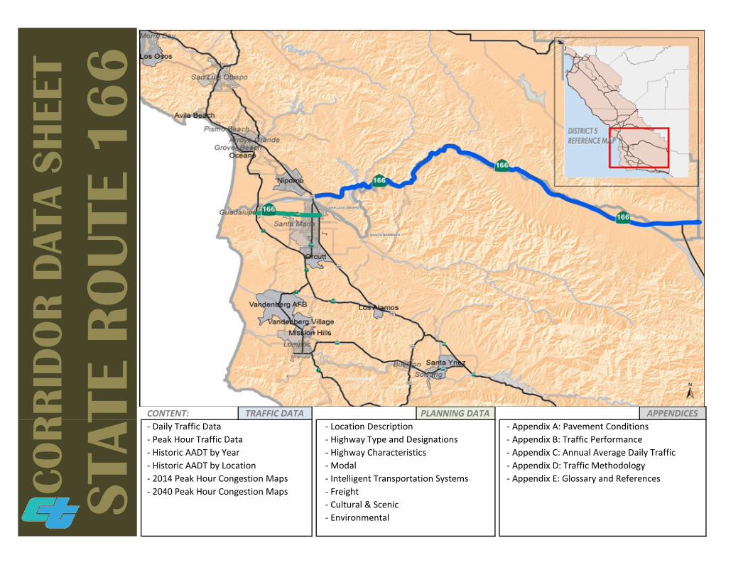
CONTENT: TRAFFIC DATA PLANNING DATA APPENDICES- Daily Traffic Data - Location Description - Appendix A: Pavement Conditions- Peak Hour Traffic Data - Highway Type and Designations - Appendix B: Traffic Performance- Historic AADT by Year - Highway Characteristics - Appendix C: Annual Average Daily Traffic- Historic AADT by Location - Modal - Appendix D: Traffic Methodology- 2014 Peak Hour Congestion Maps - Intelligent Transportation Systems - Appendix E: Glossary and References- 2040 Peak Hour Congestion Maps - Freight

- Cultural & Scenic- Environmental

CO

RR

IDO

R D

ATA

SHEE

T

STAT

E R

OU

TE 1

66

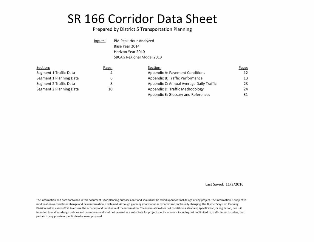
Inputs: PM Peak Hour AnalyzedBase Year 2014Horizon Year 2040SBCAG Regional Model 2013

Section: Page: Section: Page:Segment 1 Traffic Data 4 Appendix A: Pavement Conditions 12Segment 1 Planning Data 6 Appendix B: Traffic Performance 13Segment 2 Traffic Data 8 Appendix C: Annual Average Daily Traffic 23Segment 2 Planning Data 10 Appendix D: Traffic Methodology 24

Appendix E: Glossary and References 31

Last Saved: 11/3/2016

SR 166 Corridor Data SheetPrepared by District 5 Transportation Planning

The information and data contained in this document is for planning purposes only and should not be relied upon for final design of any project. The information is subject to modification as conditions change and new information is obtained. Although planning information is dynamic and continually changing, the District 5 System Planning Division makes every effort to ensure the accuracy and timeliness of the information. The information does not constitute a standard, specification, or regulation, nor is it intended to address design policies and procedures and shall not be used as a substitute for project specific analysis, including but not limited to, traffic impact studies, that pertain to any private or public development proposal.

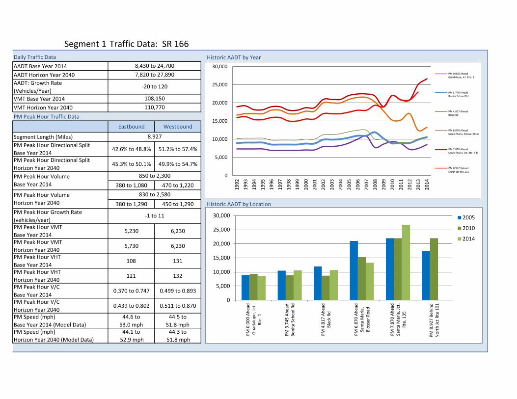
Segment 1 Traffic Data: SR 166Daily Traffic Data Historic AADT by YearAADT Base Year 2014AADT Horizon Year 2040AADT: Growth Rate (Vehicles/Year)VMT Base Year 2014VMT Horizon Year 2040

Eastbound Westbound

Segment Length (Miles)PM Peak Hour Directional Split Base Year 2014

42.6% to 48.8% 51.2% to 57.4%

PM Peak Hour Directional Split Horizon Year 2040

45.3% to 50.1% 49.9% to 54.7%

380 to 1,080 470 to 1,220

380 to 1,290 450 to 1,290 Historic AADT by LocationPM Peak Hour Growth Rate (vehicles/year)PM Peak Hour VMT Base Year 2014

5,230 6,230

PM Peak Hour VMT Horizon Year 2040

5,730 6,230

PM Peak Hour VHT Base Year 2014

108 131

PM Peak Hour VHT Horizon Year 2040

121 132

PM Peak Hour V/C Base Year 2014

0.370 to 0.747 0.499 to 0.893

PM Peak Hour V/C Horizon Year 2040

0.439 to 0.802 0.511 to 0.870

PM Speed (mph) Base Year 2014 (Model Data)

44.6 to 53.0 mph

44.5 to 51.8 mph

PM Speed (mph) Horizon Year 2040 (Model Data)

44.1 to 52.9 mph

44.3 to 51.8 mph

8,430 to 24,7007,820 to 27,890

-20 to 120

108,150110,770

PM Peak Hour Traffic Data

-1 to 11

8.927

830 to 2,580PM Peak Hour Volume Horizon Year 2040

PM Peak Hour Volume Base Year 2014

850 to 2,300 0

5,000

10,000

15,000

20,000

25,000

30,000

1992

1993

1994

1995

1996

1997

1998

1999

2000

2001

2002

2003

2004

2005

2006

2007

2008

2009

2010

2011

2012

2013

2014

PM 0.000 AheadGuadalupe, Jct. Rte. 1

PM 3.745 AheadBonita School Rd

PM 4.817 AheadBlack Rd

PM 6.870 AheadSanta Maria, Blosser Road

PM 7.870 AheadSanta Maria, Jct. Rte. 135

PM 8.927 BehindNorth Jct Rte 101

0

5,000

10,000

15,000

20,000

25,000

30,000

PM 0

.000

Ahe

adGu

adal

upe,

Jct.

Rte.

1

PM 3

.745

Ahe

adBo

nita

Sch

ool R

d

PM 4

.817

Ahe

adBl

ack

Rd

PM 6

.870

Ahe

adSa

nta

Mar

ia,

Blos

ser R

oad

PM 7

.870

Ahe

adSa

nta

Mar

ia, J

ct.

Rte.

135

PM 8

.927

Beh

ind

Nor

th Jc

t Rte

101

2005

2010

2014

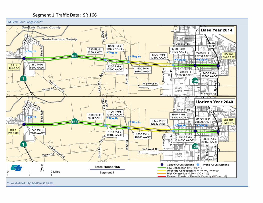
Segment 1 Traffic Data: SR 166PM Peak Hour Congestion**

Image Location:\images\166_Segment1VC.jpg

Segment DropDown Formulation Used for dropdown and table formulas0 1 Segment 1 Segment Chart Position

1 2 Segment 2 1 1

2 3456789

101112

2014 LOS # NB 2014 LOS # SB

Low 2 2High 4 4

2040 LOS # NB 2040 LOS # SB

Low 2 2High 4 4

**Last Modified: 12/22/2015 4:55:28 PM

Segment 1 Planning Data: SR 166Location Description Land UseSegment Description Image Location:Urban/Rural \images\166_Seg_1_LU.jpg

Local Planning JurisdictionCountyCityPrevalent Land Use

Highway TypeFreeway/Expressway SystemFacility TypeFunctional Classification

Highway Designations Profile LegendNational Highway SystemInterregional Road System Landscape LegendScenic Highway

Highway CharacteristicsNumber of LanesPavement Condition RightPavement Condition LeftShoulder Width Right (ft) \images\166_Seg_1_SW.jpg

Shoulder Width Left (ft)

ModalAirports ServedBicycle AccessAMTRAK Bus StationsAMTRAK Rail StationsAMTRAK Thruway BusOther Adjacent/Near FacilitiesRail/SHS CrossingsRail Crossing Description

Intelligent Transportation SystemsSignals/Mile

Shoulder Width

0Other Features: N/A

From US 101 to SR 1 (south junction)Rural

SBCAGSanta Barbara

N/AAgriculture

NoConventional/Expressway

Major Collector

NoNoNo

2-4Major/MinorMajor/Minor

0-8+0-8+

Vandenberg AFB

NoN/A

OpenN/AN/ANoNo

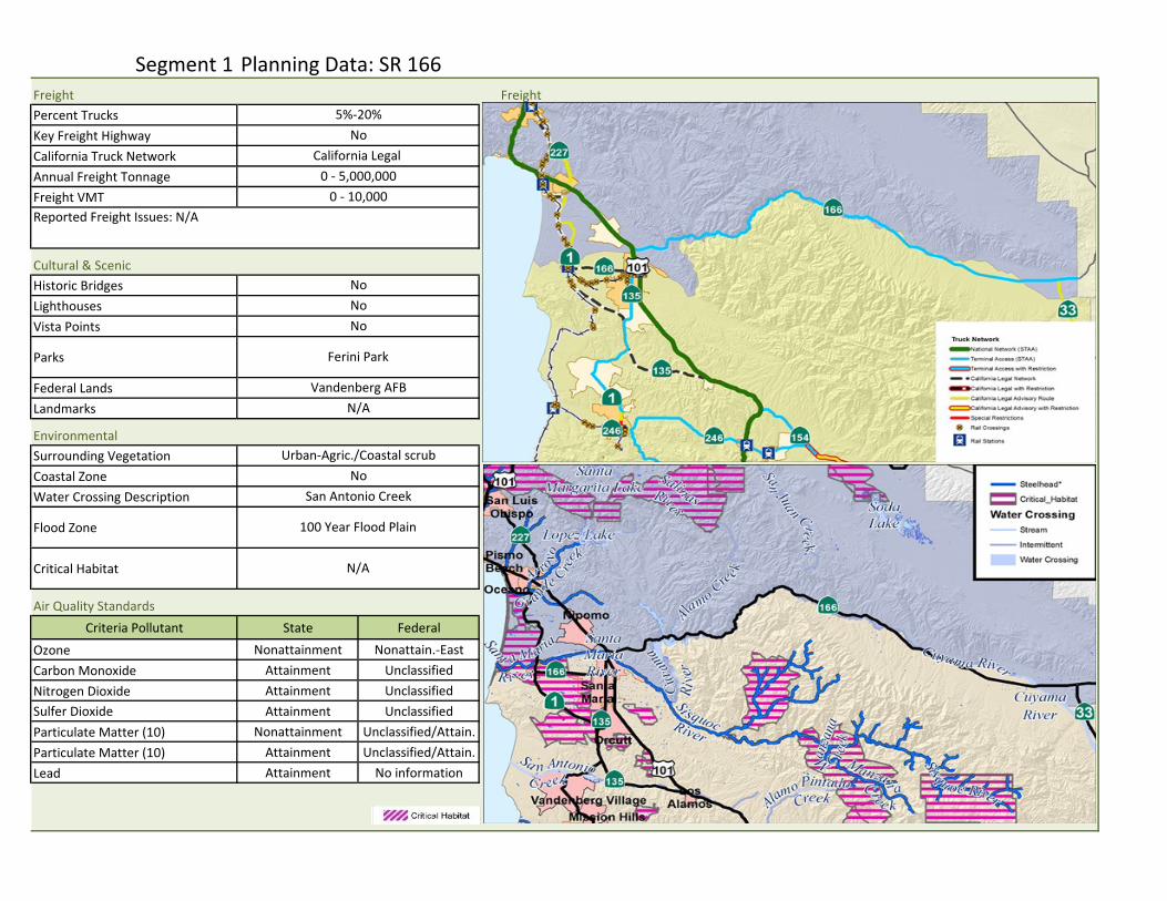
Segment 1 Planning Data: SR 166Freight FreightPercent TrucksKey Freight Highway \images\166_Seg_1_FR.jpg

California Truck NetworkAnnual Freight TonnageFreight VMT

Cultural & ScenicHistoric BridgesLighthousesVista Points

Parks

Federal LandsLandmarks

EnvironmentalSurrounding VegetationCoastal Zone Image Location:Water Crossing Description \images\166_Seg_1_CH.jpg

Flood Zone

Critical Habitat

Air Quality Standards Criteria Pollutant State Federal

Ozone Nonattainment Nonattain.-EastCarbon Monoxide Attainment UnclassifiedNitrogen Dioxide Attainment UnclassifiedSulfer Dioxide Attainment UnclassifiedParticulate Matter (10) Nonattainment Unclassified/Attain.Particulate Matter (10) Attainment Unclassified/Attain.Lead Attainment No information CH Legend

California Legal 0 - 5,000,000

0 - 10,000

5%-20%No

N/A

100 Year Flood Plain

Ferini Park

Reported Freight Issues: N/A

NoSan Antonio Creek

NoNo

Vandenberg AFBN/A

Urban-Agric./Coastal scrub

No

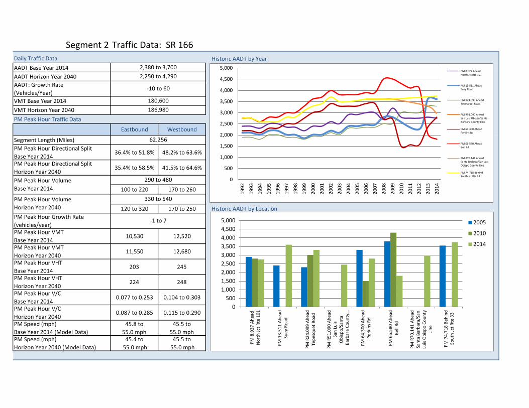
Segment 2 Traffic Data: SR 166Daily Traffic Data Historic AADT by YearAADT Base Year 2014AADT Horizon Year 2040AADT: Growth Rate (Vehicles/Year)VMT Base Year 2014VMT Horizon Year 2040

Eastbound Westbound

Segment Length (Miles)PM Peak Hour Directional Split Base Year 2014

36.4% to 51.8% 48.2% to 63.6%

PM Peak Hour Directional Split Horizon Year 2040

35.4% to 58.5% 41.5% to 64.6%

100 to 220 170 to 260

120 to 320 170 to 250 Historic AADT by LocationPM Peak Hour Growth Rate (vehicles/year)PM Peak Hour VMT Base Year 2014

10,530 12,520

PM Peak Hour VMT Horizon Year 2040

11,550 12,680

PM Peak Hour VHT Base Year 2014

203 245

PM Peak Hour VHT Horizon Year 2040

224 248

PM Peak Hour V/C Base Year 2014

0.077 to 0.253 0.104 to 0.303

PM Peak Hour V/C Horizon Year 2040

0.087 to 0.285 0.115 to 0.290

PM Speed (mph) Base Year 2014 (Model Data)

45.8 to 55.0 mph

45.5 to 55.0 mph

PM Speed (mph) Horizon Year 2040 (Model Data)

45.4 to 55.0 mph

45.5 to 55.0 mph

2,380 to 3,7002,250 to 4,290

-10 to 60

180,600186,980

PM Peak Hour Traffic Data

-1 to 7

62.256

330 to 540PM Peak Hour Volume Horizon Year 2040

PM Peak Hour Volume Base Year 2014

290 to 480 0

500

1,000

1,500

2,000

2,500

3,000

3,500

4,000

4,500

5,000

1992

1993

1994

1995

1996

1997

1998

1999

2000

2001

2002

2003

2004

2005

2006

2007

2008

2009

2010

2011

2012

2013

2014

PM 8.927 AheadNorth Jct Rte 101

PM 13.511 AheadSuey Road

PM R24.099 AheadTepesquet Road

PM R51.090 AheadSan Luis Obispo/SantaBarbara County Line

PM 64.300 AheadPerkins Rd

PM 66.580 AheadBell Rd

PM R70.141 AheadSanta Barbara/San LuisObispo County Line

PM 74.718 BehindSouth Jct Rte 33

0500

1,0001,5002,0002,5003,0003,5004,0004,5005,000

PM 8

.927

Ahe

adN

orth

Jct R

te 1

01

PM 1

3.51

1 Ah

ead

Suey

Roa

d

PM R

24.0

99 A

head

Tepe

sque

t Roa

d

PM R

51.0

90 A

head

San

Luis

Obi

spo/

Sant

aBa

rbar

a Co

unty

…

PM 6

4.30

0 Ah

ead

Perk

ins R

d

PM 6

6.58

0 Ah

ead

Bell

Rd

PM R

70.1

41 A

head

Sant

a Ba

rbar

a/Sa

nLu

is O

bisp

o Co

unty

Line

PM 7

4.71

8 Be

hind

Sout

h Jc

t Rte

33

2005

2010

2014

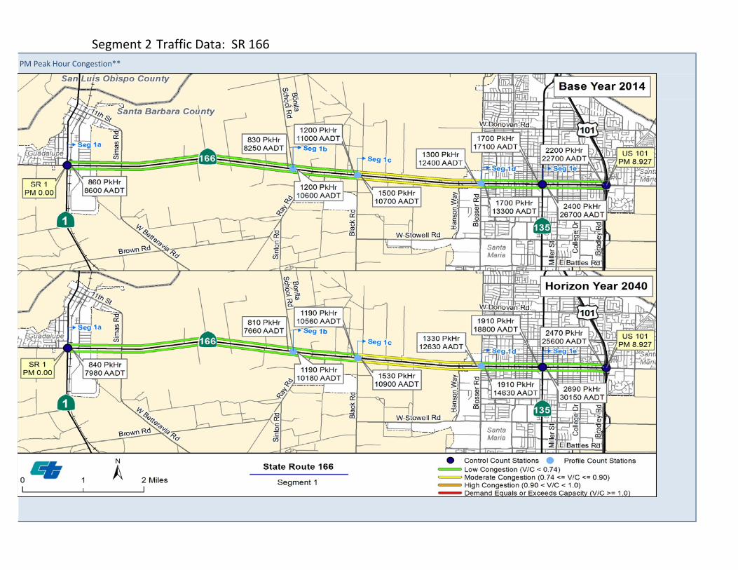
Segment 2 Traffic Data: SR 166PM Peak Hour Congestion**

Image Location:\images\166_Segment2VC.jpg

Segment DropDown Formulation Used for dropdown and table formulas0 1 Segment 1 Segment Chart Position

1 2 Segment 2 2 2

2 3456789

101112

2014 LOS # NB 2014 LOS # SB

Low 1 1High 1 1

2040 LOS # NB 2040 LOS # SB

Low 1 1High 1 1

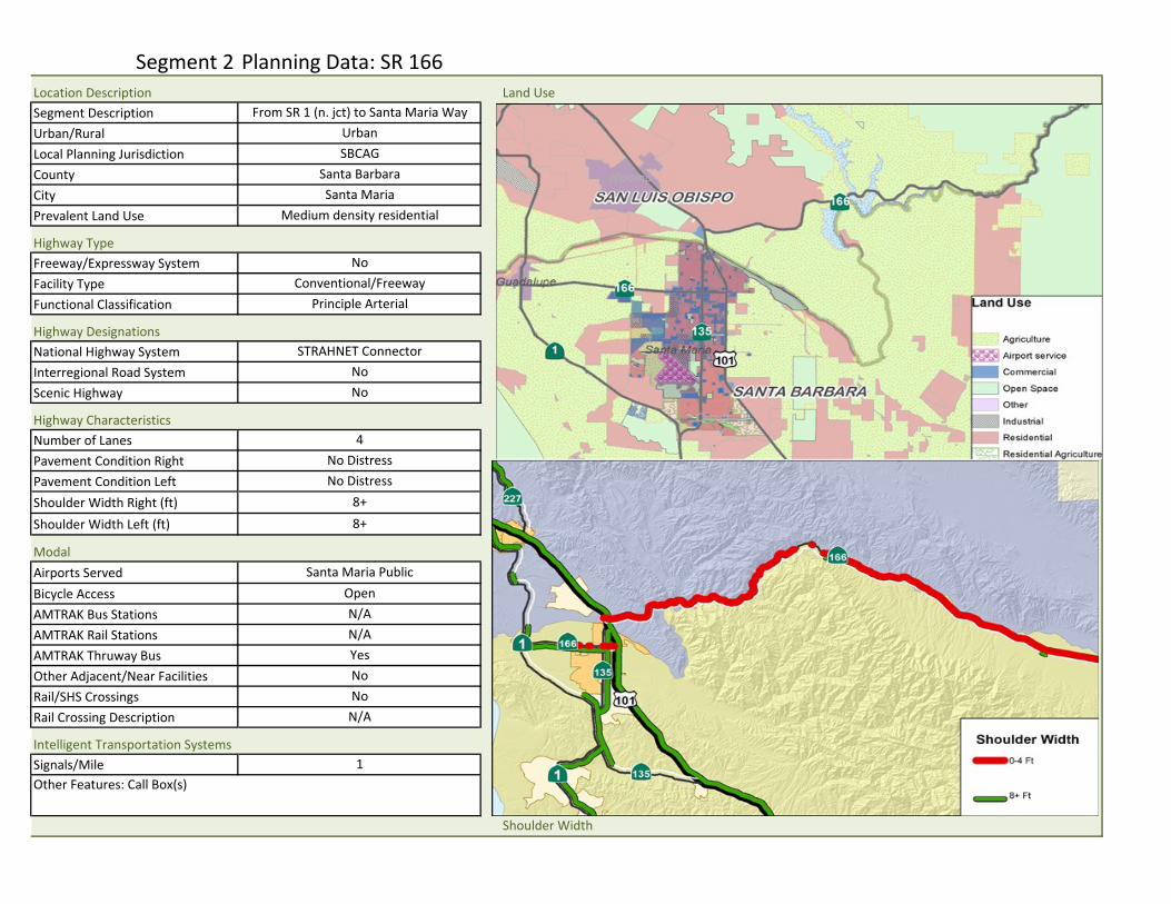
Segment 2 Planning Data: SR 166Location Description Land UseSegment Description Image Location:Urban/Rural \images\166_Seg_2_LU.jpg

Local Planning JurisdictionCountyCityPrevalent Land Use

Highway TypeFreeway/Expressway SystemFacility TypeFunctional Classification

Highway Designations Profile LegendNational Highway SystemInterregional Road System Landscape LegendScenic Highway

Highway CharacteristicsNumber of LanesPavement Condition RightPavement Condition LeftShoulder Width Right (ft) \images\166_Seg_2_SW.jpg

Shoulder Width Left (ft)

ModalAirports ServedBicycle AccessAMTRAK Bus StationsAMTRAK Rail StationsAMTRAK Thruway BusOther Adjacent/Near FacilitiesRail/SHS CrossingsRail Crossing Description

Intelligent Transportation SystemsSignals/Mile

Shoulder Width

1Other Features: Call Box(s)

From SR 1 (n. jct) to Santa Maria WayUrbanSBCAG

Santa BarbaraSanta Maria

Medium density residential

NoConventional/Freeway

Principle Arterial

STRAHNET ConnectorNoNo

4No DistressNo Distress

8+8+

Santa Maria Public

NoN/A

OpenN/AN/AYesNo

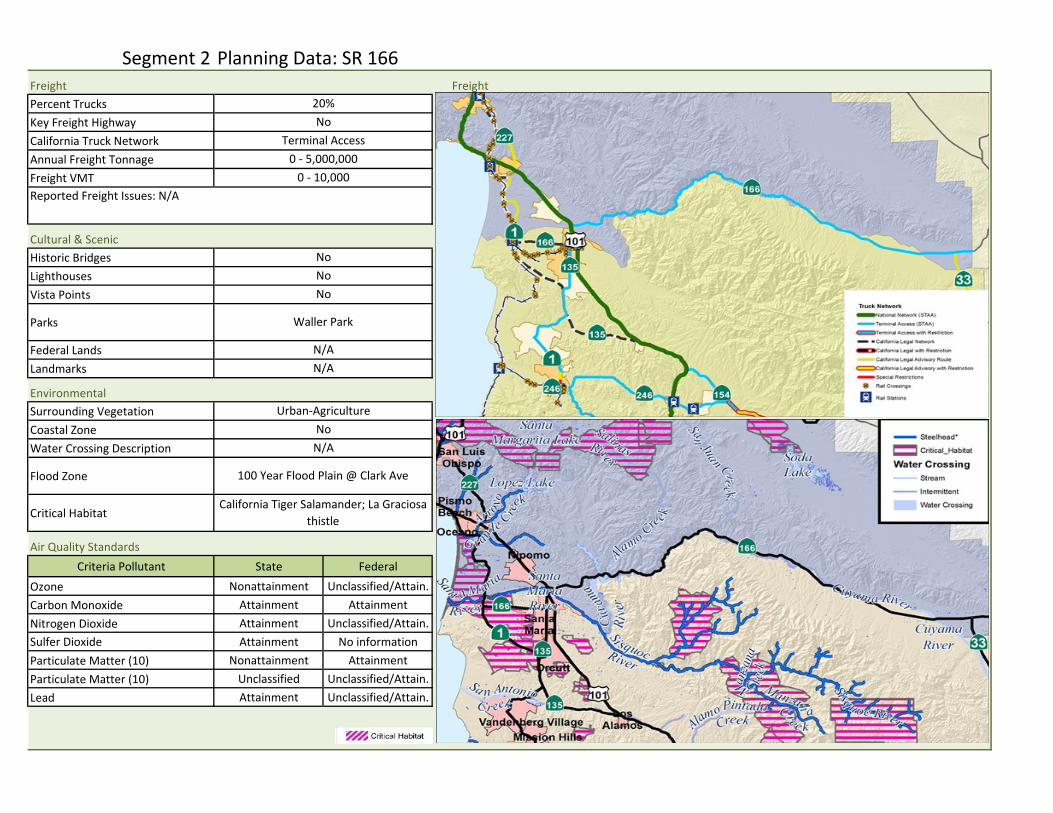
Segment 2 Planning Data: SR 166Freight FreightPercent TrucksKey Freight Highway \images\166_Seg_2_FR.jpg

California Truck NetworkAnnual Freight TonnageFreight VMT

Cultural & ScenicHistoric BridgesLighthousesVista Points

Parks

Federal LandsLandmarks

EnvironmentalSurrounding VegetationCoastal Zone Image Location:Water Crossing Description \images\166_Seg_2_CH.jpg

Flood Zone

Critical Habitat

Air Quality Standards Criteria Pollutant State Federal

Ozone Nonattainment Unclassified/Attain.Carbon Monoxide Attainment AttainmentNitrogen Dioxide Attainment Unclassified/Attain.Sulfer Dioxide Attainment No informationParticulate Matter (10) Nonattainment AttainmentParticulate Matter (10) Unclassified Unclassified/Attain.Lead Attainment Unclassified/Attain. CH Legend

Terminal Access0 - 5,000,000

0 - 10,000

20%No

California Tiger Salamander; La Graciosa thistle

100 Year Flood Plain @ Clark Ave

Waller Park

Reported Freight Issues: N/A

NoN/A

NoNo

N/AN/A

Urban-Agriculture

No

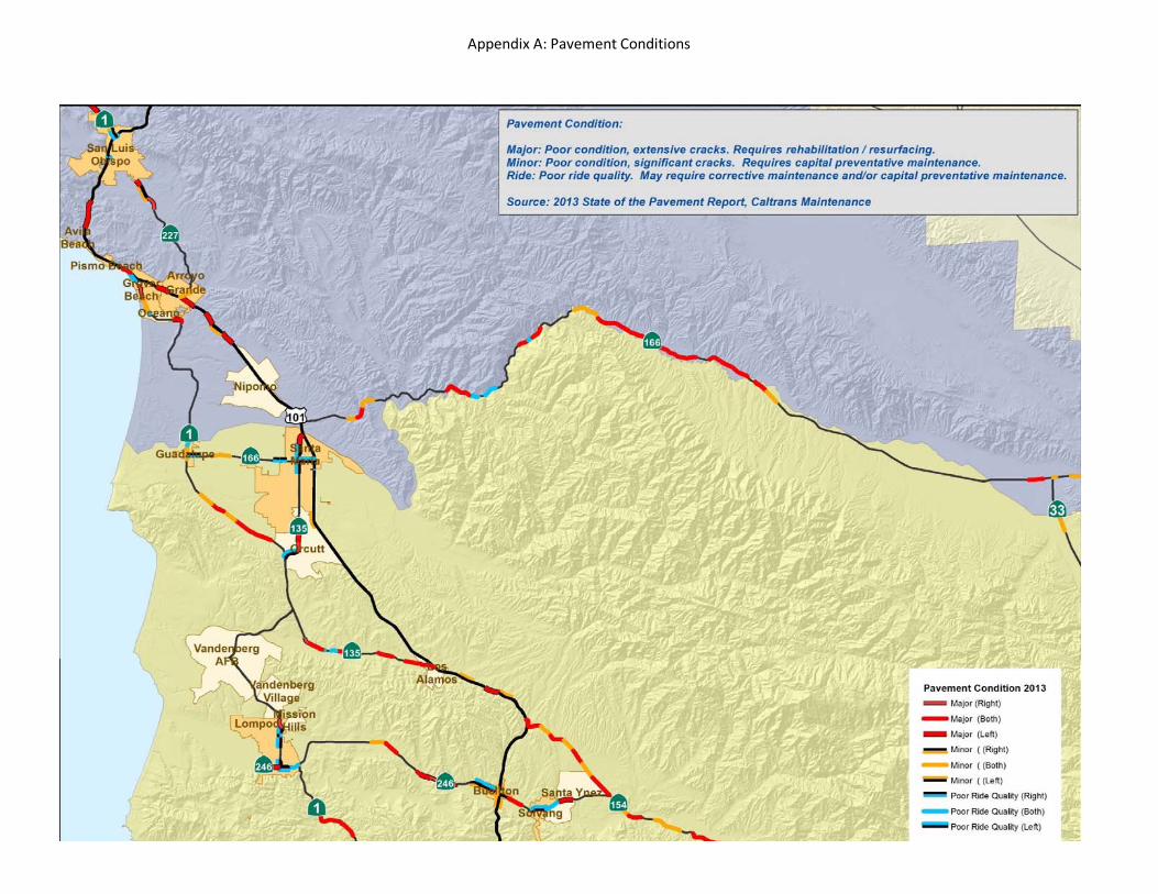
Appendix A: Pavement Conditions

\images\166_AppendixA.jpg

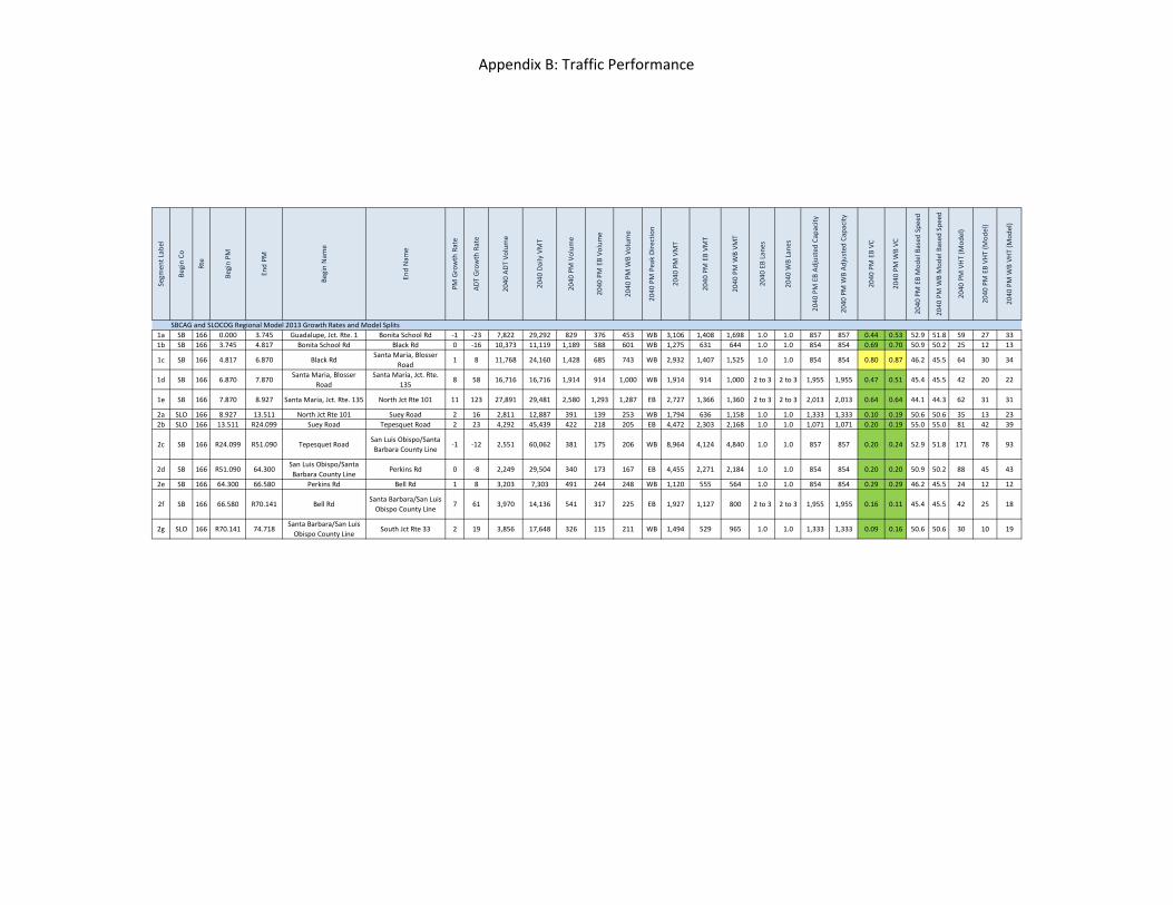
Appendix B: Traffic Performance

Segm

ent Lab

el

Begin Co

Rte

Begin PM

End PM

Begin Nam

e

End Nam

e

PM Growth Rate

ADT Growth Rate

2040

 ADT

 Volum

e

2040

 Daily VMT

2040

 PM Volum

e

2040

 PM EB Vo

lume

2040

 PM W

B Vo

lume

2040

 PM Peak Direction

2040

 PM VMT

2040

 PM EB VM

T

2040

 PM W

B VM

T

2040

 EB Lane

s

2040

 WB Lane

s

2040

 PM EB Ad

justed

 Cap

acity

2040

 PM W

B Ad

justed

 Cap

acity

2040

 PM EB VC

2040

 PM W

B VC

2040

 PM EB Mod

el Based

 Spe

ed

2040

 PM W

B Mod

el Based

 Spe

ed

2040

 PM VHT (M

odel)

2040

 PM EB VH

T (M

odel)

2040

 PM W

B VH

T (M

odel)

SBCAG and SLOCOG Regional Model 2013 Growth Rates and Model Splits1a SB 166 0.000 3.745 Guadalupe, Jct. Rte. 1 Bonita School Rd ‐1 ‐23 7,822 29,292 829 376 453 WB 3,106 1,408 1,698 1.0 1.0 857 857 0.44 0.53 52.9 51.8 59 27 331b SB 166 3.745 4.817 Bonita School Rd Black Rd 0 ‐16 10,373 11,119 1,189 588 601 WB 1,275 631 644 1.0 1.0 854 854 0.69 0.70 50.9 50.2 25 12 13

1c SB 166 4.817 6.870 Black RdSanta Maria, Blosser 

Road1 8 11,768 24,160 1,428 685 743 WB 2,932 1,407 1,525 1.0 1.0 854 854 0.80 0.87 46.2 45.5 64 30 34

1d SB 166 6.870 7.870Santa Maria, Blosser 

RoadSanta Maria, Jct. Rte. 

1358 58 16,716 16,716 1,914 914 1,000 WB 1,914 914 1,000 2 to 3 2 to 3 1,955 1,955 0.47 0.51 45.4 45.5 42 20 22

1e SB 166 7.870 8.927 Santa Maria, Jct. Rte. 135 North Jct Rte 101 11 123 27,891 29,481 2,580 1,293 1,287 EB 2,727 1,366 1,360 2 to 3 2 to 3 2,013 2,013 0.64 0.64 44.1 44.3 62 31 31

2a SLO 166 8.927 13.511 North Jct Rte 101 Suey Road 2 16 2,811 12,887 391 139 253 WB 1,794 636 1,158 1.0 1.0 1,333 1,333 0.10 0.19 50.6 50.6 35 13 232b SLO 166 13.511 R24.099 Suey Road Tepesquet Road 2 23 4,292 45,439 422 218 205 EB 4,472 2,303 2,168 1.0 1.0 1,071 1,071 0.20 0.19 55.0 55.0 81 42 39

2c SB 166 R24.099 R51.090 Tepesquet RoadSan Luis Obispo/Santa Barbara County Line

‐1 ‐12 2,551 60,062 381 175 206 WB 8,964 4,124 4,840 1.0 1.0 857 857 0.20 0.24 52.9 51.8 171 78 93

2d SB 166 R51.090 64.300San Luis Obispo/Santa Barbara County Line

Perkins Rd 0 ‐8 2,249 29,504 340 173 167 EB 4,455 2,271 2,184 1.0 1.0 854 854 0.20 0.20 50.9 50.2 88 45 43

2e SB 166 64.300 66.580 Perkins Rd Bell Rd 1 8 3,203 7,303 491 244 248 WB 1,120 555 564 1.0 1.0 854 854 0.29 0.29 46.2 45.5 24 12 12

2f SB 166 66.580 R70.141 Bell RdSanta Barbara/San Luis Obispo County Line

7 61 3,970 14,136 541 317 225 EB 1,927 1,127 800 2 to 3 2 to 3 1,955 1,955 0.16 0.11 45.4 45.5 42 25 18

2g SLO 166 R70.141 74.718Santa Barbara/San Luis Obispo County Line

South Jct Rte 33 2 19 3,856 17,648 326 115 211 WB 1,494 529 965 1.0 1.0 1,333 1,333 0.09 0.16 50.6 50.6 30 10 19

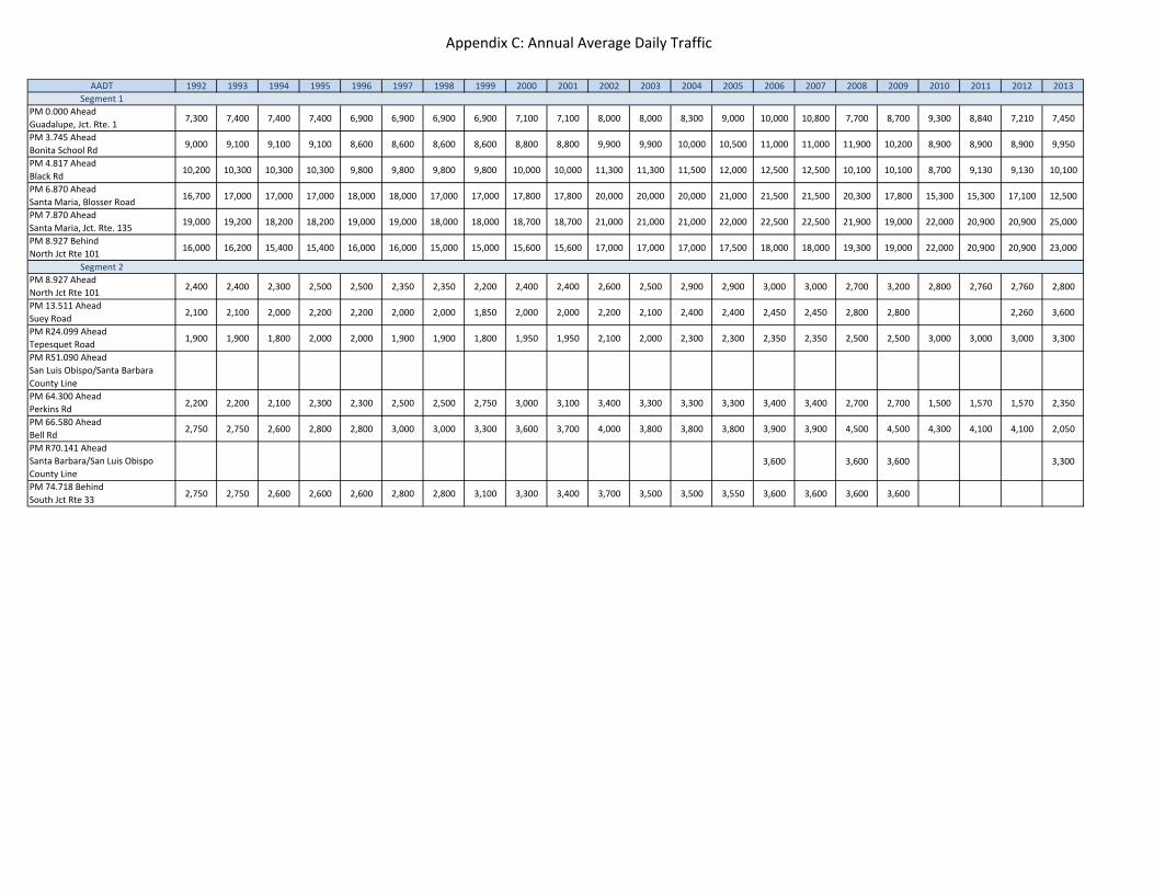
Appendix C: Annual Average Daily Traffic

AADT 1992 1993 1994 1995 1996 1997 1998 1999 2000 2001 2002 2003 2004 2005 2006 2007 2008 2009 2010 2011 2012 2013Segment 1

PM 0.000 Ahead Guadalupe, Jct. Rte. 1 7,300 7,400 7,400 7,400 6,900 6,900 6,900 6,900 7,100 7,100 8,000 8,000 8,300 9,000 10,000 10,800 7,700 8,700 9,300 8,840 7,210 7,450

PM 3.745 Ahead Bonita School Rd 9,000 9,100 9,100 9,100 8,600 8,600 8,600 8,600 8,800 8,800 9,900 9,900 10,000 10,500 11,000 11,000 11,900 10,200 8,900 8,900 8,900 9,950

PM 4.817 Ahead Black Rd 10,200 10,300 10,300 10,300 9,800 9,800 9,800 9,800 10,000 10,000 11,300 11,300 11,500 12,000 12,500 12,500 10,100 10,100 8,700 9,130 9,130 10,100

PM 6.870 Ahead Santa Maria, Blosser Road 16,700 17,000 17,000 17,000 18,000 18,000 17,000 17,000 17,800 17,800 20,000 20,000 20,000 21,000 21,500 21,500 20,300 17,800 15,300 15,300 17,100 12,500

PM 7.870 Ahead Santa Maria, Jct. Rte. 135 19,000 19,200 18,200 18,200 19,000 19,000 18,000 18,000 18,700 18,700 21,000 21,000 21,000 22,000 22,500 22,500 21,900 19,000 22,000 20,900 20,900 25,000

PM 8.927 BehindNorth Jct Rte 101 16,000 16,200 15,400 15,400 16,000 16,000 15,000 15,000 15,600 15,600 17,000 17,000 17,000 17,500 18,000 18,000 19,300 19,000 22,000 20,900 20,900 23,000

Segment 2PM 8.927 Ahead North Jct Rte 101 2,400 2,400 2,300 2,500 2,500 2,350 2,350 2,200 2,400 2,400 2,600 2,500 2,900 2,900 3,000 3,000 2,700 3,200 2,800 2,760 2,760 2,800

PM 13.511 Ahead Suey Road 2,100 2,100 2,000 2,200 2,200 2,000 2,000 1,850 2,000 2,000 2,200 2,100 2,400 2,400 2,450 2,450 2,800 2,800 #N/A #N/A 2,260 3,600

PM R24.099 Ahead Tepesquet Road 1,900 1,900 1,800 2,000 2,000 1,900 1,900 1,800 1,950 1,950 2,100 2,000 2,300 2,300 2,350 2,350 2,500 2,500 3,000 3,000 3,000 3,300

PM R51.090 Ahead San Luis Obispo/Santa Barbara County Line

#N/A #N/A #N/A #N/A #N/A #N/A #N/A #N/A #N/A #N/A #N/A #N/A #N/A #N/A #N/A #N/A #N/A #N/A #N/A #N/A #N/A #N/A

PM 64.300 Ahead Perkins Rd 2,200 2,200 2,100 2,300 2,300 2,500 2,500 2,750 3,000 3,100 3,400 3,300 3,300 3,300 3,400 3,400 2,700 2,700 1,500 1,570 1,570 2,350

PM 66.580 Ahead Bell Rd 2,750 2,750 2,600 2,800 2,800 3,000 3,000 3,300 3,600 3,700 4,000 3,800 3,800 3,800 3,900 3,900 4,500 4,500 4,300 4,100 4,100 2,050

PM R70.141 Ahead Santa Barbara/San Luis Obispo County Line

#N/A #N/A #N/A #N/A #N/A #N/A #N/A #N/A #N/A #N/A #N/A #N/A #N/A #N/A 3,600 #N/A 3,600 3,600 #N/A #N/A #N/A 3,300

PM 74.718 BehindSouth Jct Rte 33 2,750 2,750 2,600 2,600 2,600 2,800 2,800 3,100 3,300 3,400 3,700 3,500 3,500 3,550 3,600 3,600 3,600 3,600 #N/A #N/A #N/A #N/A

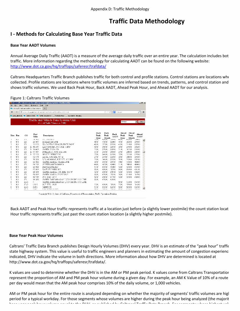
Appendix D: Traffic Methodology

Traffic Data Methodology

I ‐Methods for Calculating Base Year Traffic Data 

Base Year AADT Volumes

Annual Average Daily Traffic (AADT) is a measure of the average daily traffic over an entire year. The calculation includes bottraffic. More information regarding the methodology for calculating AADT can be found on the following website:  http://www.dot.ca.gov/hq/traffops/saferesr/trafdata/

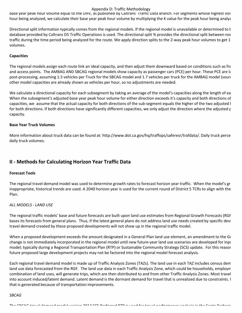
Caltrans Headquarters Traffic Branch publishes traffic for both control and profile stations. Control stations are locations whecollected. Profile stations are locations where traffic volumes are inferred based on trends, patterns, and control station and shows traffic volumes. We used Back Peak Hour, Back AADT, Ahead Peak Hour, and Ahead AADT for our analysis.

Figure 1: Caltrans Traffic Volumes

Back AADT and Peak Hour traffic represents traffic at a location just before (a slightly lower postmile) the count station locatiHour traffic represents traffic just past the count station location (a slightly higher postmile).

Base Year Peak Hour Volumes

Caltrans' Traffic Data Branch publishes Design Hourly Volumes (DHV) every year. DHV is an estimate of the “peak hour” trafficstate highway system. This value is useful to traffic engineers and planners in estimating the amount of congestion experienceindicated, DHV indicate the volume in both directions. More information about how DHV are determined is located at http://www.dot.ca.gov/hq/traffops/saferesr/trafdata/.

K values are used to determine whether the DHV is in the AM or PM peak period. K values come from Caltrans Transportationrepresent the proportion of AM and PM peak hour volume during a given day. For example, an AM K Value of 10% of a route per day would mean that the AM peak hour comprises 10% of the daily volume, or 1,000 vehicles. 

AM or PM peak hour for the entire route is analyzed depending on whether the majority of segments' traffic volumes are highperiod for a typical workday. For those segments whose volumes are higher during the peak hour being analyzed (the majoritbase year peak hour volume equal to the DHV as published by Caltrans' Traffic Data Branch For segments whose highest volu

Appendix D: Traffic Methodologybase year peak hour volume equal to the DHV, as published by Caltrans' Traffic Data Branch. For segments whose highest voluhour being analyzed, we calculate their base year peak hour volume by multiplying the K value for the peak hour being analyz

Directional split information typically comes from the regional models. If the regional model is unavailable or determined to bdatabase provided by Caltrans D5 Traffic Operations is used. The directional split % provides the directional split between nortraffic during the time period being analyzed for the route. We apply direction splits to the 2‐way peak hour volumes to get 1‐volumes.

Capacities

The regional models assign each route link an ideal capacity, and then adjust them downward based on conditions such as freand access points.  The AMBAG AND SBCAG regional models show capacity as passenger cars (PCE) per hour. These PCE are lapost‐processing, assuming 1.5 vehicles per Truck for the SBCAG model and 1.7 vehicles per truck for the AMBAG model (sourcother model capacities are already shown as vehicles per hour, so no adjustments are needed.

We calculate a directional capacity for each subsegment by taking an average of the model's capacities along the length of eaWhen the subsegment's adjusted base year peak hour volume for either direction exceeds it's capacity and both directions ofcapacities, we  assume that the actual capacity for both directions of the sub‐segment equals the higher of the two adjusted bfor both directions. If both directions have significantly different capacities, we only adjust the direction where the adjusted pcapacity.

Base Year Truck Volumes

More information about truck data can be found at: http://www.dot.ca.gov/hq/traffops/saferesr/trafdata/. Daily truck percedaily truck volumes.

II ‐Methods for Calculating Horizon Year Traffic Data

Forecast Tools

The regional travel demand model was used to determine growth rates to forecast horizon year traffic.  When the model's groinappropriate, historical trends are used. A 2040 horizon year is used for the current round of District 5 TCRs to align with thePlan.

ALL MODELS ‐ LAND USE

The regional traffic models’ base and future forecasts are built upon land use estimates from Regional Growth Forecasts (RGFbases its forecasts from general plans.  Thus, if the latest general plans do not address land use needs created by specific devetravel demand created by these proposed developments will not show up in the regional traffic model.  

When a proposed development exceeds the amount designated in a General Plan land use element, an amendment to the Gechange is not immediately incorporated in the regional model until new future‐year land use scenarios are developed for inpumodel; typically during a Regional Transportation Plan (RTP) or Sustainable Community Strategy (SCS) update.  For this reasonfuture proposed large development projects may not be factored into the regional model forecast analysis.

Each regional travel demand model is made up of Traffic Analysis Zones (TAZs). The land use in each TAZ includes census demland use data forecasted from the RGF.  The land use data in each Traffic Analysis Zone, which could be households, employmcombination of land uses, will generate trips, which are then distributed to and from other Traffic Analysis Zones. Most travelinto account induced/latent demand. Latent demand is the dormant demand for travel that is unrealized due to constraints. Ithat is generated because of transportation improvements.

SBCAG

The SBCAG travel demand model version 2013 SCS Preferred RTP is used for travel performance analysis in the Santa Barbara

Appendix D: Traffic MethodologyThe SBCAG travel demand model version 2013 SCS Preferred RTP is used for travel performance analysis in the Santa BarbaraPreferred RTP model incorporates Sustainable Community Strategies in future year scenarios and was adopted by the SBCAG accepted by the California Air Resources Board on November 21, 2013 (source: http://sbcag.org/planning/2040RTP/Calendar2040.

SLOCOG

The SLOCOG 2014 RTP/SCS was adopted in April, 2015. The SLOCOG travel demand model accounts for: SB 375, Sustainable Cfuture demand reduction strategies such as ridesharing, vanpools and public transit. They use a horizon year of 2035.  

AMBAG

The AMBAG travel demand model is used for travel performance analysis in the Monterey, Santa Cruz and San Benito regionsSustainable Community Strategies in future year scenarios. The AMBAG regional travel demand model developed for the MTyear and incorporates Sustainable Community Strategies. The AMBAG RTP‐SCS was adopted by the AMBAG Board in June 201

CALTRANS HISTORICAL COUNTS

Caltrans historical traffic counts can be used to develop growth rates using linear regression analysis, but the regional modelstraffic counts are shown graphically over time and over space by segment in the Route Data Sheet. For segment and sub‐segmmeasures that use AADT and peak hour traffic as inputs, we take the average of back and ahead volumes between count statin calculating performance measures such as V/C, VMT, VHT, speed and LOS.

Historical Growth Rate

Where model growth rates are deemed inappropriate, historical growth rates are used to project Caltrans base year counts to

Model Growth Rate

Regional model growth rates were used to project base year counts to horizon year traffic volumes.

The regional model analyzes mainline volumes at a macro level, and it has not been validated or calibrated to a project level aused in a micro‐level analysis such as calculating turning movement volumes and intersection level of service which would beoperational analysis.  The regional model is used as a basis to develop inputs for the micro level analysis.Regional model outputs reflect traffic patterns during a typical Tuesday thru Thursday.  The regional models include AM and PPeak hour volumes are typically analyzed because they are typically higher than the AM Peak period. 

Adjusted Model Growth Rate

The future AADT and peak hour volumes are forecasted using growth rates estimated from model volumes. These model volfuture year, are adjusted to correct for differences between base year Caltrans' counts and base year model volumes. The mostep assumptions, such as the household travel surveys, trip rate assumptions, mode split formulations, and travel delay funcestimate of the expected travel patterns. Therefore, although the model has been validated and calibrated, the base year moperfectly to Caltrans' counts.

The base year model volume is always adjusted to match the base year count. The future year model volumes can be adjustevolume adjustment methods described in NCHRP Report 255. The ratio and difference methods are defined by equations (1) method is applied by taking the average result of the ratio and difference methods. 

Appendix D: Traffic Methodology

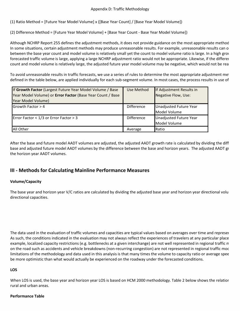
(1) Ratio Method = [Future Year Model Volume] x ([Base Year Count] / [Base Year Model Volume])

(2) Difference Method = [Future Year Model Volume] + [Base Year Count ‐ Base Year Model Volume]) 

Although NCHRP Report 255 defines the adjustment methods, it does not provide guidance on the most appropriate methodIn some situations, certain adjustment methods may produce unreasonable results. For example, unreasonable results can obetween the base year count and model volume is relatively small yet the count to model volume ratio is large. In a high growforecasted traffic volume is large, applying a large NCHRP adjustment ratio would not be appropriate. Likewise, if the differencount and model volume is relatively large, the adjusted future year model volume may be negative, which would not be rea

To avoid unreasonable results in traffic forecasts, we use a series of rules to determine the most appropriate adjustment metdefined in the table below, are applied individually for each sub‐segment volume. In most cases, the process results in use of 

After the base and future model AADT volumes are adjusted, the adjusted AADT growth rate is calculated by dividing the diffbase and adjusted future model AADT volumes by the difference between the base and horizon years. The adjusted AADT grthe horizon year AADT volumes.  

III ‐Methods for Calculating Mainline Performance Measures

Volume/Capacity

The base year and horizon year V/C ratios are calculated by dividing the adjusted base year and horizon year directional volumdirectional capacities. 

If Growth Factor (Largest Future Year Model Volume / Base Year Model Volume) or Error Factor (Base Year Count / Base Year Model Volume)

Use Method If Adjustment Results in Negative Flow, Use:

Growth Factor > 4 Difference Unadjusted Future Year Model Volume

Error Factor < 1/3 or Error Factor > 3 Difference Unadjusted Future Year Model Volume

All Other Average Ratio

The data used in the evaluation of traffic volumes and capacities are typical values based on averages over time and represenAs such, the conditions indicated in the evaluation may not always reflect the experiences of travelers at any particular placeexample, localized capacity restrictions (e.g. bottlenecks at a given interchange) are not well represented in regional traffic mon the road such as accidents and vehicle breakdowns (non‐recurring congestion) are not represented in regional traffic modlimitations of the methodology and data used in this analysis is that many times the volume to capacity ratio or average speebe more optimistic than what would actually be experienced on the roadway under the forecasted conditions.

LOS

When LOS is used, the base year and horizon year LOS is based on HCM 2000 methodology. Table 2 below shows the relationrural and urban areas.

Performance Table

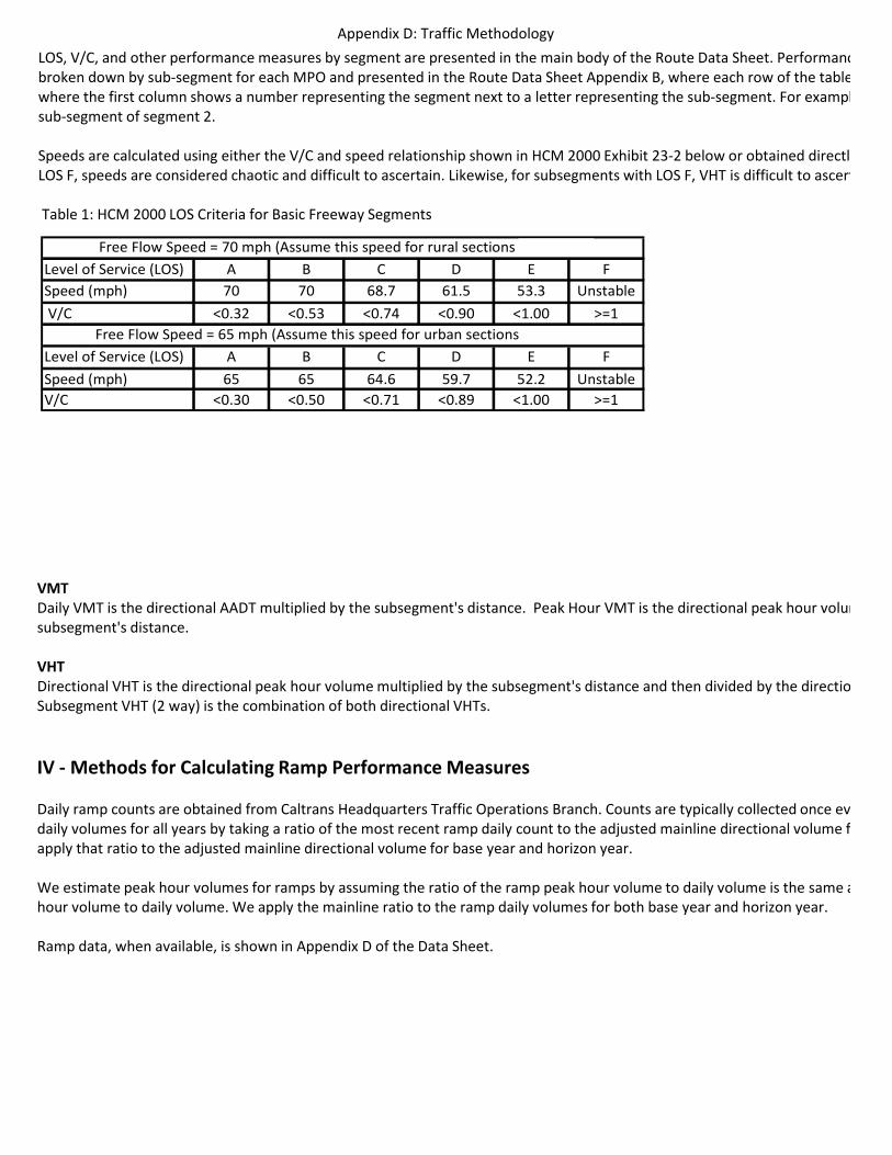
Appendix D: Traffic MethodologyLOS, V/C, and other performance measures by segment are presented in the main body of the Route Data Sheet. Performancbroken down by sub‐segment for each MPO and presented in the Route Data Sheet Appendix B, where each row of the tablewhere the first column shows a number representing the segment next to a letter representing the sub‐segment. For examplsub‐segment of segment 2. 

Speeds are calculated using either the V/C and speed relationship shown in HCM 2000 Exhibit 23‐2 below or obtained directlyLOS F, speeds are considered chaotic and difficult to ascertain. Likewise, for subsegments with LOS F, VHT is difficult to ascert

Table 1: HCM 2000 LOS Criteria for Basic Freeway Segments

VMTDaily VMT is the directional AADT multiplied by the subsegment's distance.  Peak Hour VMT is the directional peak hour volumsubsegment's distance. 

VHTDirectional VHT is the directional peak hour volume multiplied by the subsegment's distance and then divided by the directioSubsegment VHT (2 way) is the combination of both directional VHTs.

IV ‐Methods for Calculating Ramp Performance Measures

Daily ramp counts are obtained from Caltrans Headquarters Traffic Operations Branch. Counts are typically collected once evdaily volumes for all years by taking a ratio of the most recent ramp daily count to the adjusted mainline directional volume fapply that ratio to the adjusted mainline directional volume for base year and horizon year.

We estimate peak hour volumes for ramps by assuming the ratio of the ramp peak hour volume to daily volume is the same ahour volume to daily volume. We apply the mainline ratio to the ramp daily volumes for both base year and horizon year.

Ramp data, when available, is shown in Appendix D of the Data Sheet.

Level of Service (LOS) A B C D E FSpeed (mph) 70 70 68.7 61.5 53.3 Unstable V/C <0.32 <0.53 <0.74 <0.90 <1.00 >=1

Level of Service (LOS) A B C D E FSpeed (mph) 65 65 64.6 59.7 52.2 UnstableV/C <0.30 <0.50 <0.71 <0.89 <1.00 >=1

Free Flow Speed = 70 mph (Assume this speed for rural sections of SR‐101)

Free Flow Speed = 65 mph (Assume this speed for urban sections of SR‐101)