Embed Size (px)
Citation preview

CORPORATE INVESTMENT, FINANCING AND PAYOUT DECISIONS:
EVIDENCE FROM UK-LISTED COMPANIES
by
QINGWEI MENG
A thesis submitted to the
University of Birmingham
for the degree of
DOCTOR OF PHILOSOPHY
Department of Accounting and Finance
Birmingham Business School
University of Birmingham
September 2012

University of Birmingham Research Archive
e-theses repository This unpublished thesis/dissertation is copyright of the author and/or third parties. The intellectual property rights of the author or third parties in respect of this work are as defined by The Copyright Designs and Patents Act 1988 or as modified by any successor legislation. Any use made of information contained in this thesis/dissertation must be in accordance with that legislation and must be properly acknowledged. Further distribution or reproduction in any format is prohibited without the permission of the copyright holder.
Abstract
– i –
ABSTRACT
The research reported in this doctoral thesis aims to contribute to the corporate finance
literature by focusing on the interdependence of corporate investment, financing and payout
decisions of UK-listed companies, within the period 1999–2008. The thesis consists of six
chapters. After the introductory chapter, Chapter 2 critically reviews the existing theoretical
and empirical literature on corporate investment, financing and payout policies, from which
several promising research ideas are identified. Chapter 3 investigates the interactions among
the three corporate decisions. One of the key findings is that the three corporate decisions are
likely to be jointly determined in the presence of financial constraints. The results also suggest
that the effect of uncertainty on corporate investment is significantly positive, but the effect
on dividend payout is significantly negative. Chapter 4 explores the influence of managerial
confidence and economic sentiment on the set of jointly determined corporate decisions. An
important finding is that the state of confidence at aggregate levels has significantly positive
effects on both real investment and debt financing decisions. Chapter 5 discriminates
conceptually and evaluates empirically twenty alternative measures of corporate investment
used in the existing literature. It is found that conclusions drawn from empirical analyses are
likely to be sensitive to the choice of corporate investment measures, indicating that the
measurement of corporate investment behaviour matters. The key findings of the thesis are
summarised in the conclusion chapter, alongside some promising ideas for further research.

Dedication
– ii –
DEDICATION
To my dear parents
for all of your love and support

Acknowledgements
– iii –
ACKNOWLEDGEMENTS
This thesis has been made possible through the support and assistance of many individuals
and organisations. I therefore wish to acknowledge the following in producing this thesis.
My greatest intellectual indebtedness is to Professor Victor Murinde and Dr. Ping
Wang, my supervisor and co-supervisor, for their excellent guidance, valuable advice and
continuous support throughout my PhD programme. They have provided me with helpful
suggestions, not only for my research work, but also for my career development. My sincere
gratitude also goes to Professor Christopher J. Green and Dr. Paul Cox, my external and internal
examiners, for offering critical and constructive comments on the final draft of this thesis.
I wish to express my sincere gratitude to Birmingham Business School and the
Graduate School of the University of Birmingham for providing me with valuable academic
support during the course of my study, and for sponsoring me to present my research papers at
the 18th Global Finance Conference in Bangkok, Thailand; the 18th Multinational Finance
Conference in Rome, Italy; the 8th Applied Financial Economics Conference in Samos,
Greece; the 19th Global Finance Conference in Chicago, USA; and the 19th Multinational
Finance Conference in Krakow, Poland.
I would like to extend my gratitude to the discussants and participants at the Global
Finance Conference 2011 and 2012, Multinational Finance Conference 2011 and 2012,
Applied Financial Economics Conference 2011, Midlands Regional Doctoral Colloquium

Acknowledgements
– iv –
2010 and 2011, ESRC seminar 2009 as well as research seminars held at the African
Development Bank and Birmingham Business School for their valuable comments and
constructive suggestions on the previous versions of the papers presented in this thesis.
Special thanks to the Global Finance Association for awarding the paper entitled “Corporate
investment, financing and payout decisions under financial constraints and uncertainty:
evidence from UK panel data” the Best Paper Award; the College of Social Science of the
University of Birmingham for awarding the above paper the Best Doctoral Research Paper
Award; and the Midlands Doctoral Colloquium for awarding the paper entitled “The
measurement of corporate investment matters: evidence from UK panel data” the Best Paper
Award. The papers mentioned above are based on earlier versions of Chapters 3 and 5
presented in this thesis respectively.
I am grateful to the academic staff and my fellow PhD students in the Corporate
Finance Research Group at Birmingham Business School who have also commented on my
work, especially Professor Robert Cressy and Dr. Hisham Farag. Furthermore, I wish to thank
all my colleagues and friends who helped me, motivated me, and made my stay in the UK
enjoyable and unforgettable.
Finally, and most importantly, I am deeply indebted to my dear parents, Xianhua
Meng and Yuzhen Shi, for their unconditional support with love and patience over the years.
This study would not have reached its conclusion without their encouragement and
inspiration.

Table of Contents
– v –
TABLE OF CONTENTS
Abstract i
Dedication ii
Acknowledgements iii
List of Tables x
List of Figures xii
List of Appendices xiii
Chapter 1: Introduction 1
1.1 Background and motivation 1
1.2 Data and methodology 5
1.3 Structure and scope of the thesis 9
Chapter 2: Literature Review 14
2.1 Introduction 14
2.2 Corporate decision theories 18
2.2.1 Corporate investment theories 18
2.2.2 Corporate financing theories 29
2.2.3 Dividend payout theories 37
2.3 Simultaneity of corporate decisions 48
2.3.1 Institutional approach 49
2.3.2 Flow-of-funds framework for corporate behaviour 51
2.3.3 Information approach 54
2.3.4 Tax approach 57
2.3.5 Agency approach 60
2.4 Corporate decisions under uncertainty 63
Table of Contents
– vi –
2.4.1 Corporate investment decision and uncertainty 64
2.4.2 Corporate financing decision and uncertainty 74
2.4.3 Corporate payout decision and uncertainty 76
2.5 Corporate decisions and managerial confidence 77
2.5.1 Modern corporate finance versus behavioural corporate finance 77
2.5.2 Corporate investment decision and managerial confidence 82
2.5.3 Corporate financing decision and managerial confidence 85
2.5.4 Corporate payout decision and managerial confidence 89
2.6 Conclusion and promising research ideas 92
2.6.1 Conclusion 92
2.6.2 Promising research ideas 95
Chapter 3: Corporate Decisions, Financial Constraints and Uncertainty 111
3.1 Introduction 111
3.2 Empirical proxies for uncertainty 114
3.2.1 Output volatility 115
3.2.2 Input volatility 117
3.2.3 Profit volatility 118
3.2.4 Stock returns volatility 119
3.2.5 Macroeconomic volatility 121
3.3 An information asymmetry-based flow-of-funds framework for corporate behaviour 123
3.4 Modelling corporate investment, financing and payout behaviour 130
3.4.1 Corporate investment equation 130
3.4.2 Debt financing equation 131
3.4.3 Dividend payout equation 133
3.5 Data and preliminary analysis 134
3.5.1 Data and measurement 134
Table of Contents
– vii –
3.5.2 Preliminary diagnostic tests 142
3.6 Empirical results and implications for corporate behaviour 150
3.6.1 Single equation analyses 150
3.6.2 Simultaneous equations analyses 167
3.6.3 Long-run solution to the simultaneous equations system 174
3.7 Robustness tests and further evidence 178
3.7.1 Robustness tests and results 178
3.7.2 Further evidence on the simultaneity of corporate decisions 180
3.8 Concluding remarks 186
Chapter 4: Corporate Decisions, Managerial Confidence and Economic Sentiment 201
4.1 Introduction 201
4.2 Measures of managerial confidence and economic sentiment 205
4.2.1 Sector-specific managerial confidence indicators 207
4.2.2 Economic sentiment indicators 214
4.3 Modelling corporate behavioural equations 222
4.3.1 Corporate behavioural equations with proxy for the state of confidence 222
4.3.2 Corporate behavioural equations with confidence and uncertainty variables 226
4.4 Data and preliminary analysis 228
4.5 Empirical results and implications for corporate behaviour 234
4.5.1 Simultaneous analyses with proxy for the state of confidence 236
4.5.2 Simultaneous analyses with confidence and uncertainty variables 244
4.6 Robustness tests and further evidence 251
4.6.1 Robustness tests and results 251
4.6.2 Further evidence on the influence of managerial confidence on corporate behaviour 253
4.7 Concluding remarks 262
Table of Contents
– viii –
Chapter 5: The Measurement of Corporate Investment Behaviour Matters 282
5.1 Introduction 282
5.2 Empirical measures of corporate investment behaviour 285
5.2.1 Cash based versus accrual based corporate investment measures 287
5.2.2 Gross versus net corporate investment measures 293
5.2.3 Book versus replacement values of capital stock 296
5.2.4 Contemporaneous versus lagged proxies for capital stock 297
5.2.5 Conclusion 298
5.3 Development of hypotheses 302
5.3.1 Hypotheses regarding whether the measurement of investment matters 302
5.3.2 Hypotheses regarding the volatility of investment measures 304
5.3.3 Hypotheses regarding the information content of investment measures 305
5.4 Data and preliminary analysis 307
5.4.1 Data and measurement 307
5.4.2 Summary statistics 308
5.4.3 Correlation coefficient analysis 313
5.5 A simple regression of Tobin’s Q model of investment 318
5.5.1 Empirical procedures 319
5.5.2 Empirical results 320
5.5.3 Robustness tests and results 325
5.5.4 Conclusion 326
5.6 Trend analysis 327
5.6.1 Empirical procedures 327
5.6.2 Empirical results 330
5.6.3 Robustness tests and results 337
5.6.4 Conclusion 338
5.7 Information content analysis 339
Table of Contents
– ix –
5.7.1 Incremental and relative information content 340
5.7.2 Empirical procedures 343
5.7.3 Empirical results 346
5.7.4 Robustness tests and results 351
5.7.5 Conclusion 352
5.8 Concluding remarks 354
Chapter 6: Conclusion 385
6.1 Summary 385
6.2 Key empirical findings and conclusions 386
6.2.1 Simultaneous determination of corporate decisions 386
6.2.2 Corporate decisions under uncertainty 388
6.2.3 Corporate decisions and the state of confidence 389
6.2.4 Measurement of corporate investment behaviour 392
6.3 Main contributions to the existing literature 394
6.4 Practical implications of the findings 397
6.4.1 Implications for corporate managers 398
6.4.2 Implications for public policy makers 399
6.4.3 Implications for investors 401
6.5 Limitations of the research 402
6.6 Promising ideas for further research 404
References 408
List of Appendices
– x –
LIST OF TABLES
Table 3.1: Endogenous corporate decision variables and hypothesised interactions under the flow-of-funds framework for corporate behaviour 129
Table 3.2: Description of main variables used in Chapter 3 136
Table 3.3: Descriptive statistics for main variables used in Chapter 3 139
Table 3.4: Correlation coefficient matrix of variables used in Chapter 3 141
Table 3.5: Tests for equality of uses and sources of funds 145
Table 3.6: Endogeneity tests for corporate decision variables 147
Table 3.7: Endogeneity test for cash flow variable 149
Table 3.8: System-GMM estimation results for corporate investment equation with uncertainty 155
Table 3.9: System-GMM estimation results for corporate financing equation with uncertainty 160
Table 3.10: System-GMM estimation results for corporate dividend equation with uncertainty 164
Table 3.11: 3SLS estimation results for investment, financing and payout equations with uncertainty 169
Table 3.12: Long-run solution to the simultaneous equations system 176
Table 3.13: 3SLS estimation results for corporate behavioural equations with uncertainty using subsamples 182
Table 4.1: Descriptive statistics for sector-specific confidence and economic sentiment indicators 219
Table 4.2: Correlation coefficient matrix of the UK and EU sector-specific confidence and economic sentiment indicators 221
Table 4.3: Description of main variables used in Chapter 4 229
List of Appendices
– xi –
Table 4.4: Descriptive statistics for main variables used in Chapter 4 231
Table 4.5: Correlation coefficient matrix of variables used in Chapter 4 233
Table 4.6: 3SLS estimation results for corporate behavioural equations with sector-specific managerial confidence 239
Table 4.7: 3SLS estimation results for corporate behavioural equations with economic sentiment 243
Table 4.8: 3SLS estimation results for corporate behavioural equations with company-level uncertainty and sector-specific managerial confidence 247
Table 4.9: 3SLS estimation results for corporate behavioural equations with company-level uncertainty and economic sentiment 249
Table 4.10: 3SLS estimation results for corporate behavioural equations with sector-specific managerial confidence interacted with sector dummies 256
Table 4.11: 3SLS estimation results for corporate behavioural equations with company-level uncertainty and sector-specific managerial confidence interacted with sector dummies 259
Table 5.1: Corporate investment measures and representative recent studies 300
Table 5.2: Summary statistics for corporate investment measures examined in Chapter 5 309
Table 5.3: Pearson correlation coefficients of alternative corporate investment measures 316
Table 5.4: System-GMM estimation results for Tobin’s Q model of corporate investment 321
Table 5.5: System-GMM estimation results for the trend regression of corporate investment measures 331
Table 5.6: Coefficients of variation of the root mean square error of the corporate investment measures 335
Table 5.7: System-GMM estimation results for the regression of stock returns on unexpected earnings and unexpected corporate investment 347
Table 5.8: Volatility-information content matrix for corporate investment measures 353

List of Appendices
– xii –
LIST OF FIGURES
Figure 1.1: Flowchart for the research methodology of this study 6
Figure 4.1: Time series plot of UK versus EU manufacturing sector confidence indicators 211
Figure 4.2: Time series plot of UK versus EU services sector confidence indicators 211
Figure 4.3: Time series plot of UK versus EU consumer confidence indicators 212
Figure 4.4: Time series plot of UK versus EU retail trade sector confidence indicators 212
Figure 4.5: Time series plot of UK versus EU construction sector confidence indicators 213
Figure 4.6: Time series plot of UK versus EU economic sentiment indicators 217
Figure 5.1: Logical relation between incremental and relative information content of two variables 341

List of Appendices
– xiii –
LIST OF APPENDICES
Appendix 2.A: Corporate investment theories and representative recent empirical evidence 99
Appendix 2.B: Capital structure theories and representative recent empirical evidence 102
Appendix 2.C: Dividend policy theories and representative recent empirical evidence 106
Appendix 2.D: Methodologies and findings of selected literature on simultaneity of corporate decisions 110
Appendix 3.A: Key findings from Chapter 3 versus findings from prior research 188
Appendix 3.B: 2SLS estimation results for investment, financing and payout equations with uncertainty 193
Appendix 3.C: 3SLS estimation results for investment, financing and payout equations without uncertainty 195
Appendix 3.D: 3SLS estimation results for investment, financing and payout equations with alternative measure of uncertainty UNC2 197
Appendix 3.E: 3SLS estimation results for investment, financing and payout equations with alternative measure of uncertainty UNC3 199
Appendix 4.A: Sample sizes of the Joint Harmonised EU Business and Consumer Surveys 264
Appendix 4.B: EU Programme of Business and Consumer Surveys 265
Appendix 4.C: 3SLS estimation results for corporate behavioural equations with sector-specific managerial confidence at year end 272
Appendix 4.D: 3SLS estimation results for corporate behavioural equations with economic sentiment at year end 274
Appendix 4.E: 3SLS estimation results for corporate behavioural equations with changes in economic sentiment 276

List of Appendices
– xiv –
Appendix 4.F: 2SLS estimation results for corporate behavioural equations with sector-specific managerial confidence 278
Appendix 4.G: 2SLS estimation results for corporate behavioural equations with economic sentiment 280
Appendix 5.A: Perpetual inventory method for estimating the replacement value of capital stock 358
Appendix 5.B: Mean-comparison test results for alternative corporate investment measures 359
Appendix 5.C: Time series plot of annual mean values of corporate investment measures 361
Appendix 5.D: Spearman’s rank correlation coefficients of alternative corporate investment measures 364
Appendix 5.E: Difference-GMM estimation results for Tobin’s Q model of corporate investment 366
Appendix 5.F: System-GMM estimation results for Tobin’s Q model of corporate investment without dynamic structure 369
Appendix 5.G: System-GMM estimation results for Tobin’s Q model of corporate investment with alternative measure of Q 372
Appendix 5.H: Rankings of the corporate investment measures based on an alternative measure of volatility 375
Appendix 5.I: Difference-GMM estimation results for the trend regression of corporate investment measures 376
Appendix 5.J: Coefficients of variation of the root mean square error based on difference-GMM estimation results 379
Appendix 5.K: Fixed effect estimation results for the regressions of stock returns on unexpected earnings and unexpected corporate investment 380
Appendix 5.L: System-GMM estimation results for the regressions of stock returns on unexpected earnings and alternative measure of unexpected corporate investment 382
Chapter 1: Introduction
– 1 –
CHAPTER 1
INTRODUCTION
1.1 Background and motivation
Corporate investment, financing and payout choices are known as the trilogy of corporate
decisions (see Wang, 2010), and are believed to have significant influence on corporate
performance. They have attracted great attention in the existing literature (see, for example,
Denis and Osobov, 2008; Almeida and Campello, 2007; Frank and Goyal, 2003; Baker et al.,
2002; among many others). Companies use internal and external funds to finance their
investment projects, in an attempt to maximise their company value and thus shareholders’
wealth. Internal funds are chiefly represented by retained earnings and non-cash expenses;
and external funds mainly refer to the proceeds from issuing new debt and new equity.
Managers, therefore, have to make both real (i.e. non-financial) and financial decisions. The
real decisions are concerned with the optimal level of capital investment; while financial
decisions are concerned with how to finance the desired investment, which involves the
appraisal of two financial choices. One is dividend payout choice, i.e. how much internally
generated funds should be paid out to shareholders as dividends which otherwise could be
re-invested in the business. The other is external financing choice, i.e. how much external
funds does a company need to raise from outside capital markets for its investment.
Although much effort has been devoted to investigating the corporate behaviour of

Chapter 1: Introduction
– 2 –
companies, the three corporate decisions are typically discussed separately and routinely
examined in isolation rather than altogether. Indeed, the seminal works by Modigliani and
Miller (1958) and Miller and Modigliani (1961) posit separately the investment separation
principle, capital structure irrelevance theorem and dividend irrelevance theorem (hereafter
the Modigliani-Miller theorems). The Modigliani-Miller theorems demonstrate that internal
and external funds for a company are perfect substitutes in a perfect market environment, and
hence the company’s optimal level of investment should be determined solely by its real
considerations and totally independent of its financial decisions. Both capital structure and
dividend payout choices, thus, should have no impact on company value, and be irrelevant to
shareholders’ wealth, suggesting no interdependencies among the set of corporate decisions
within a perfect market environment. As a result, each of the three corporate decisions has
been widely and intensively scrutinised in the existing corporate finance literature, but we
know little about the interactions that may exist among them.
Prior research, however, has provided reasons and evidence that financial constraints
in the real world, such as insufficient availability of internal funds and limited access to new
external funds, may hamper companies’ ability to invest efficiently (see, for example, Fazzari
et al., 1988; and Guariglia, 2008). It is true that in practice the corporate decisions are related
through the accounting identity, in that sources of funds must equal uses of funds. So when a
company adjusts any one policy, the other policies may also be affected. Therefore,
companies should consider their investment decisions alongside their fund-raising choices.
Chapter 1: Introduction
– 3 –
Although no consensus has been reached, an important implication is that corporate
investment, financing and payout decisions are likely to be interdependent upon one another
and jointly determined by management. The single equation frameworks used by prior
research without explicitly accounting for the interdependence among corporate decisions
may be misspecified, which potentially leads to incomplete and biased results. A simultaneous
equations framework, therefore, is likely to provide greater insight into the inter-relationships
that may exist among the set of corporate decisions, improving our knowledge of corporate
decision-making processes in the real world. It is worth highlighting that, by referring to the
simultaneous determination of corporate decisions throughout the thesis, we are by no means
arguing that corporate decisions are necessarily made at the same time, but rather that they are
likely to be executed on simultaneously so that the outcomes can be observed via a
simultaneous approach.
Recent literature that seeks to explore the determinants of corporate investment
behaviour has highlighted the importance of uncertainty associated with companies’ future
prospects, even though the investment-uncertainty relationship remains theoretically
ambiguous and empirically inconclusive (see, for example, Carruth et al., 2000; Lensink and
Murinde, 2006; and Baum et al., 2008). However, the potential effects of uncertainty on
corporate financing and payout decisions have received little attention. Given the fact that all
corporate decisions are made on the basis of incomplete information and a company’s future
cash flows are likely to be uncertain, it is reasonable to argue that the degree of uncertainty

Chapter 1: Introduction
– 4 –
matters in both corporate financing and payout decisions as well. If this is true, uncertainty
may influence investment, not only on its own, but also through its effects on financing and
payout choices. Prior research on corporate investment under uncertainty that ignore the roles
played by financing and payout choices should be critically reviewed, since they may
generate misleading results and lead to inappropriate inferences. It is, therefore, more
plausible to model corporate investment, financing and payout decisions simultaneously, and
to investigate the effect of uncertainty on the set of corporate decisions systematically.
Moreover, recent developments suggest that behavioural finance plays an important
role in explaining aspects of finance that traditional finance literature has failed to explain.
Behavioural finance literature replaces the traditional assumption of broad rationality with a
potentially more realistic assumption that agents’ behaviours are less than fully rational. The
assumption of less than full rationality finds strong support from a large body of
psychological literature (see, for example, Gilovich et al., 2002). The behavioural finance
approach is now commonly used in asset pricing literature, in which investors are assumed to
be less than fully rational. Corporate finance literature, however, rarely relaxes the assumption
that managers are fully rational. Although the theoretical framework in this emerging area has
not been firmly established and the empirical evidence is still relatively rare (see Baker et al.,
2006), it is plausible to hypothesise that the less than fully rational manager approach to
behavioural corporate finance has the potential to explain a wide range of patterns in
companies’ investment, financing and payout choices. This thesis, therefore, also extends the
Chapter 1: Introduction
– 5 –
existing corporate finance literature by incorporating the state of managerial confidence and
economic sentiment into corporate behavioural models in an attempt to provide new insights
into the influence of managers’ psychological bias on aspects of corporate behaviour.
1.2 Data and methodology
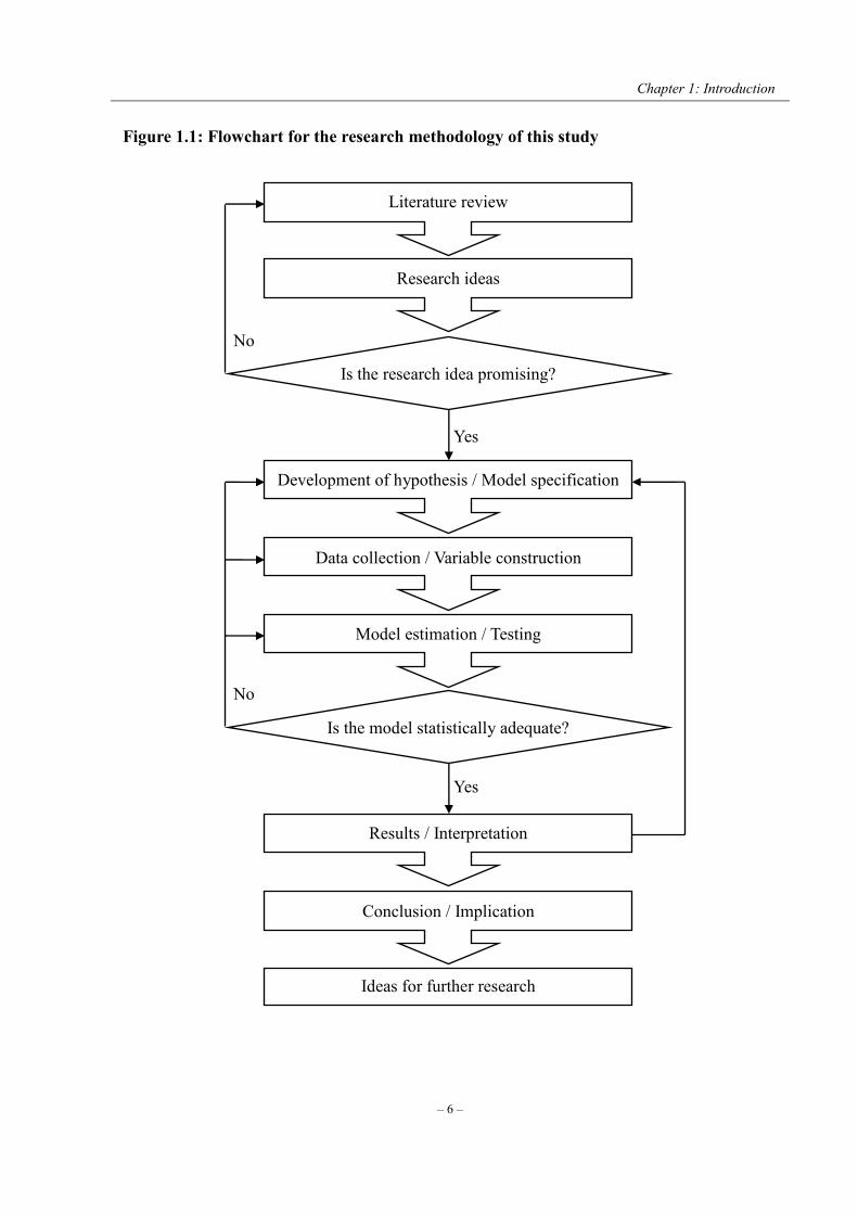
The research methodology adopted by this study is described in Figure 1.1, using a simple
flowchart. It starts with a comprehensive and critical review of the existing literature, which is
not only helpful in understanding the relevant context of this study, but also useful for
identifying the potential gaps in the previous studies from which a number of research ideas
are proposed. The promising research ideas are used to develop testable hypotheses and to
formulate empirical models.
The data used in this study are collected from different sources, which are mainly
secondary and thus available electronically through financial and economic information
providers. Specifically, accounting and financial data for the companies listed on the London
Stock Exchange (LSE) within the period from 1999 to 2008 are retrieved from the
Worldscope database via Thomson One Banker Analytics. Stock price data for the same batch
of companies over the same period of time are collected from the DataStream database. The
indicators for managerial confidence and economic sentiment are publicly available from the
European Commission Economic Database. Worldscope is chosen as the principal data source
since it is the most comprehensive web-based database covering accounting and financial
information for companies from 130 exchanges, including the LSE listed companies.
Chapter 1: Introduction
– 6 –
Figure 1.1: Flowchart for the research methodology of this study
Literature review
Research ideas
Is the research idea promising?
No
Yes
Development of hypothesis / Model specification
Data collection / Variable construction
Model estimation / Testing
No
Is the model statistically adequate?
Yes
Results / Interpretation
Conclusion / Implication
Ideas for further research

Chapter 1: Introduction
– 7 –
At the data collection stage, as many companies, years and items as possible are
collected to form our dataset in order to prevent the need for extra data collection at later
stages. The initial dataset has more than 30,000,000 data entries. There are, however, some
variations among the sample sizes used in different empirical works presented in this thesis,
depending on the objectives of the studies, the specifications of the models as well as the
estimation techniques adopted. A detailed description of the sampling procedures employed to
construct the final samples is given in each of the empirical chapters.
UK-listed companies are chosen as the sample for this thesis because it is argued that
financial constraints on corporate investment are relatively more severe in the more
market-oriented UK financial system than in the continental European financial system (see,
for example, Bond et al., 2003; and Seitfert and Gonenc, 2008). Bond et al. (2003) indicate
that, compared with the continental European financial market, the market-oriented financial
system in the UK perform less well in channelling investment funds to companies with
profitable investment opportunities because of the arm’s-length relation between companies
and suppliers of finance. The market-oriented financial system in the UK thus may give rise
to financial constraints for the UK-listed companies. Moreover, Seifert and Gonenc (2008)
point out that the ownership of the UK-listed companies is considerably dispersed as
compared to companies in other markets. Because of the relatively widespread ownership of
stock, investors in the UK face more severe problems of information asymmetry, which may
also give rise to financial constraints. Therefore, the interactions among corporate investment,
Chapter 1: Introduction
– 8 –
financing and payout decisions are likely to be more pronounced for the UK-listed companies
which tend to be characterised by severe financial constraints. Besides, this study focus on the
corporate decisions made by the UK-listed companies over the period 1999–2008 which
allow us to sidestep the data breaks that characterise the period 2009–2012.
The dataset is organised as a panel which has both cross-company and time-series
dimensions. The pooling of company-year observations provides a more informative dataset
which enables us to tackle the complexity of corporate decision-making procedures by
relaxing the assumptions that are implicitly made in pure cross-sectional or pure time-series
analysis (see, for example, Baltagi, 2008; and Brooks, 2008). Therefore, the rich structure
makes the panel dataset intuitively more preferable than pure cross-sectional and pure
time-series data in the context of empirical corporate finance research.
The empirical models formulated in this thesis are estimated using a number of
estimation techniques for panel data, including fixed effect, random effect, first-difference
generalised method of moments (difference-GMM), system generalised method of moments
(system-GMM), two-stage least squares (2SLS) and three-stage least squares (3SLS)
estimations. The choice of estimation methods largely depends on the model specification, the
sampling procedure and the results from statistical tests. Diagnostic tests and robustness
checks are also carried out to statistically evaluate the estimation results. If a model is not
statistically adequate, either the model will be reformulated or a different estimation technique
will be used. The process of building a statistically adequate and robust model, therefore, is an

Chapter 1: Introduction
– 9 –
iterative one, as illustrated in Figure 1.1. The empirical results obtained from estimating
statistically adequate models are interpreted with reference to theoretical predictions.
Overall, the main research methodology adopted by this thesis is empirical. The thesis
as a whole is structured following the steps described in Figure 1.1. Besides this, the empirical
papers presented in Chapters 3, 4 and 5 are also structured in such a way as to ensure a good
understanding of the existing literature, promising research ideas, solid theoretical
frameworks, a sufficiently large dataset, appropriate econometric techniques, testing for
robustness of empirical results, credible interpretations, and thus reliable findings and
conclusions. A detailed methodology is provided in each of the empirical chapters.
1.3 Structure and scope of the thesis
The thesis consists of six chapters, including an introduction, a literature review chapter, three
stand-alone empirical chapters and a conclusion. The remainder of the thesis is structured as
follows.
Chapter 2 critically reviews the existing literature, both theoretical and empirical, on
corporate investment, financing and payout policies. Corporate finance theories about the
three key corporate decisions are briefly reviewed respectively, together with recent empirical
evidence, in order to explore the current state of knowledge on aspects of corporate behaviour.
More importantly, some prior studies attempt to examine how various frictions in the real
world may drive linkages among corporate investment, financing and payout decisions. The
mechanisms through which the set of corporate decisions may affect one another are explored

Chapter 1: Introduction
– 10 –
in detail. Furthermore, since uncertainty has been identified as a key determinant of corporate
investment, Chapter 2 comprehensively reviews literature on the effect of uncertainty on
corporate investment decisions as well as its potential effects on corporate financing and
payout decisions. In addition, following the recent argument that managers’ psychological
bias may explain a wide range of patterns in corporate behaviour that traditional corporate
finance literature has failed to explain, Chapter 2 also reviews the small but growing strand of
literature on behavioural corporate finance. Based on the literature reviewed in Chapter 2,
several promising research ideas are proposed, aiming to fill the critical lacunae identified in
the existing corporate finance literature.
Chapter 3 presents the first empirical work. It investigates the interactions among
corporate investment, financing and payout decisions under financial constraints and
uncertainty, using a large panel of UK-listed companies. We model these corporate decisions
within a simultaneous equations system which explicitly allows for contemporaneous
interdependence among them, as implied by the information asymmetry-based flow-of-funds
framework for corporate behaviour. It is found that capital investment and dividend payout, as
competing uses of funds, are negatively interrelated, but both are positively related to the net
amount of new debt issued, which may imply joint determination of corporate decisions under
financial constraints. We also offer the first attempt to examine simultaneously the effects of
uncertainty on the three corporate decisions. The results show that the effect of uncertainty on
corporate investment is significant and positive, while the effect on dividend payouts is

Chapter 1: Introduction
– 11 –
significant and negative. Furthermore, the results suggest that financial constraints may
intensify simultaneity among corporate decisions, and reduce managerial flexibility to
respond to uncertainty.
Chapter 4 presents the second empirical work. It extends the work presented in
Chapter 3 by taking into account the role of the state of confidence in the determination of
corporate decisions. The relations between corporate decisions and the state of confidence are
examined within the simultaneous equations system formulated in Chapter 3. It is found that
the state of confidence at aggregate level, as proxied by UK or EU sector-specific managerial
confidence indicators or overall economic sentiment indicators, has significantly positive
effects on companies’ real investment and debt financing decisions. The significant effects of
the state of confidence on investment and financing decisions persist even after controlling for
company idiosyncratic uncertainty and other company-specific fundamental characteristics.
However, corporate payout decisions are mainly affected by company idiosyncratic
uncertainty rather than confidence at sector level or sentiment at economy level. Besides, the
results also show that, compared with the companies in the other sectors, UK-listed
companies in the services sector behave more aggressively when the managerial confidence
or economic sentiment is high. Specifically, they invest in capital stock more intensively, use
debt financing more heavily, and cut dividends more decisively when their managers are
confident. Chapter 4 contributes to the small but growing literature on behavioural corporate
finance, providing evidence that managers’ psychological bias plays an important role in the
Chapter 1: Introduction
– 12 –
determination of corporate decisions.
Chapter 5 presents the third empirical work. The survey of corporate finance literature
shows that use of corporate investment to capital stock ratio as a measure of corporate
investment behaviour has been common practice in empirical analyses. Although the
corporate investment measures used in the literature seem, at first sight, to be very similarly
specified, they in fact vary in terms of the numerator and the denominator, i.e. how
investment spending and capital stock are empirically measured. However, there is no
literature that provides a comparison among the various versions of the corporate investment
ratios, and thus we know little about how differently these corporate investment measures
perform in empirical analyses. As a result, a claim has been implicitly made that the different
measures of corporate investment can always yield equivalent results in corporate investment
research. The purpose of Chapter 5, therefore, is to conceptually discriminate and statistically
evaluate twenty alternative measures of corporate investment ratios which have been
identified in the existing literature. Simple statistical and econometric procedures are utilised
to test the sensitivity of the conclusions drawn from empirical analyses to choice of corporate
investment measures. It is found that corporate investment measures with different
specifications are not uniformly positively correlated with one another. Significantly negative
correlations are also observed among the alternative measures, which appear surprising, since
they are supposed to measure the investment behaviour of the same batch of companies over
the same period of time. A simple regression of the Tobin’s Q model clearly shows that the
Chapter 1: Introduction
– 13 –
choice of corporate investment measures, to a considerable extent, influences the conclusions
drawn from empirical analyses. Furthermore, the relative performances of the alternative
corporate investment measures, in terms of volatility and information content, are empirically
evaluated. Empirical results suggest that gross investment measures are less volatile around
their respective trends and thus are more predictable compared with net investment measures,
while cash based investment measures contain greater value relevant information than their
accrual based counterparts. Accordingly, cash based gross investment measures, which
contain relatively less noise and greater value relevant information, are recommended to
researchers for future studies, if they have to make a mutually exclusive choice among the
alternatives without any particular preference.
Chapter 6 concludes this thesis by recapping the research questions, summarising the
key findings, highlighting the main contributions, discussing the broad implications and
acknowledging the limitations. A number of promising ideas for future research are also
proposed in Chapter 6.
Chapter 2: Literature Review
– 14 –
CHAPTER 2
LITERATURE REVIEW
2.1 Introduction
Investment, financing and payout choices are the three important corporate decisions that
have attracted much attention in the literature for more than half century (see, for example,
Denis and Osobov, 2008; Almeida and Campello, 2007; Frank and Goyal, 2003; and Baker et
al., 2002). The seminal works by Modigliani and Miller (1958) and Miller and Modigliani
(1961), i.e. the Modigliani-Miller theorems, show that, in a perfect market environment,
internal and external funds are perfect substitutes for companies to finance their investment,
and hence the optimal level of investment should be solely determined by the real
considerations and totally independent of the financial decisions.1
Since the seminal works by Modigliani and Miller, researchers have tried to explain
how real world complications alter perfect and efficient capital market conditions, and how
market imperfections make corporate financing and payout choices relevant to investment
decisions and company value. By relaxing Modigliani-Miller’s assumptions and introducing
1 The Modigliani-Miller theorems are generally considered as a cornerstone of modern corporate finance, so we shall not go into the details of the seminal works. Suffice it to say here that Modigliani-Miller’s assumptions include the existence of risk class (i.e. each company belongs to a risk class), neutral taxes (i.e. all types of tax payer and all sources of income are taxed at the same rate), no capital market frictions (i.e. no transaction costs, no bankruptcy costs, no flotation costs and no asset trade restrictions), symmetrical access to credit markets (i.e. the same borrowing and lending rate for companies and investors); corporate financial policy contains no information (i.e. financial choices cannot be used to convey any signal about a company’s value to investors), etc.
Chapter 2: Literature Review
– 15 –
market imperfections, corporate finance research has intensively scrutinised each of the three
corporate decisions. Although much effort has been devoted to investigating the corporate
behaviour of companies, these three corporate decisions are typically discussed separately and
routinely examined in isolation. For example, empirical investigations of corporate
investment decisions commonly utilise a single equation framework in which a corporate
investment measure is regressed on a set of exogenous explanatory variables, without
explicitly accounting for the interdependence of various other policies, such as financing and
payout choices. Similar approaches are also used to investigate corporate financing and
payout decisions. In practice, however, corporate decision-making is a complex process, in
which the decisions made by one department are likely to be affected by those made by others
(Mueller, 1967). As argued by Fazzari et al. (1988), financial constraints, such as insufficient
availability of internal finance and limited access to external finance, may hamper companies’
ability to invest efficiently. Under such conditions, companies have to consider their
fund-raising choices alongside investment decisions; that is, if any one policy is adjusted,
other polices must also be adjusted accordingly (Gatchev et al., 2010). However, our
knowledge about the potential interactions among the corporate decisions is limited by the
single equation framework currently used in the literature, which is unable to capture the
simultaneous determination of corporate decisions and fails to provide a complete view of
corporate behaviour. It should be borne in mind that the simultaneous determination corporate
decision refers to the execution, or outcome, of the set of corporate decisions rather than the
Chapter 2: Literature Review
– 16 –
actual decision-making process.
Conventional literature on corporate finance has also been criticised for overlooking
the effects of uncertainty on companies’ real and financial behaviours. Recent studies that
seek to explore the determinants of corporate investment have highlighted the importance of
uncertainty associated with companies’ prospects (see, for example, Baum et al., 2008;
Lensink and Murinde, 2006; and Carruth et al., 2000). Several channels through which
uncertainty may influence investment have been identified and examined. Nonetheless, the
relationship between investment and uncertainty remains theoretically ambiguous and
empirically inconclusive. Compared with corporate investment decisions, the importance of
uncertainty in financing and payout decisions has received little attention, and consequently
the influence of uncertainty on investment through its effects on financing and payout choices
has also been largely ignored. The omission of relevant information in examining the effect of
uncertainty on corporate investment is likely to generate misleading results and lead to
inappropriate inferences, casting doubt on the conclusions drawn from the exiting literature on
the investment-uncertainty relationship.
More recently, behaviour finance has begun to play an important role in explaining
aspects of finance that traditional finance literature has failed to explain. Behavioural finance
literature replaces the traditional assumption of broad rationality with a potentially more
realistic behavioural assumption that agents’ behaviours are less than fully rational, i.e. they
may have behavioural biases (Baker et al., 2006). Prior research in this area has mainly

Chapter 2: Literature Review
– 17 –
focused on the influence of investors’ psychological bias, by adopting the less than fully
rational investor approach to behavioural corporate finance. However, it is argued that
managers’ psychological bias may also have a substantial impact on corporate decisions (see,
for example, Malmendier et al., 2011; Oliver and Mefteh, 2010; Hackbarth, 2008; and Heaton,
2002). In particular, managers’ upward bias towards future company performance may
generate overinvestment, underinvestment and pecking order financing behaviours through
different mechanisms. Although the theoretical framework in this emerging area has not been
firmly established and the empirical evidence is still relatively rare, the existing literature
shows that the less than fully rational manager approach has the potential to explain a wide
range of patterns in companies’ investment, financing and payout choices which conventional
corporate finance literature has failed to explain.
The remainder of this chapter proceeds as follows. Section 2.2 briefly reviews
mainstream corporate finance theories on investment, financing and payout decisions
respectively, alongside their empirical evidence. Section 2.3 explores the possible channels
through which the three corporate decisions may be interdependent upon one another and thus
jointly determined by management. Section 2.4 surveys both theoretical and empirical studies
on the effects of uncertainty on investment decisions as well as on the financial decisions of
companies. Section 2.5 focuses on the behavioural corporate finance literature and the
relationships between managerial confidence and corporate decisions. Concluding remarks as
well as promising research ideas are offered in Section 2.6.

Chapter 2: Literature Review
– 18 –
2.2 Corporate decision theories
2.2.1 Corporate investment theories
Corporate investment decision is one of the fundamental decisions made by individual
companies to risk their funds, in the hope of producing streams of revenue in the future. The
best-known method of determining whether an investment should be undertaken is the
standard net present value (NPV) rule. Its principle is fairly simple, that is, discount both
expected future cash inflow and outflow of a project back to their present value at a specific
discount rate, and then sum them up to obtain the NPV of the project. All projects with
positive NPV would add value to shareholders’ wealth and should be accepted, while all
projects with negative NPV would damage company value and should be rejected.
The NPV rule, on the one hand, has been widely used throughout the business world.
Graham and Harvey (2001) report that 74.9% of the Chief Financial Officers (CFOs)
surveyed rely heavily on this technique for evaluating investment projects. One the other hand,
it has long been acknowledged that the application of the NPV rule in capital investment
practices is not without critique. As noted in Dixit and Pindyck (1994), discount rates set by
companies to evaluate investment opportunities are typically three or four times the cost of
capital. More recently, Ow-Yong and Murinde (2009) survey a sample of 159 UK
non-financial companies listed on the London Stock Exchange. They find that a
theory-practice gap still exists in terms of the non-usage of discounted cash flow techniques.
Arnold and Hatzopoulos (2000) argue that the theory-practice gap in capital budgeting is
Chapter 2: Literature Review
– 19 –
partly due to the impractical assumptions underlying the NPV rule. As a result, the NPV rule
provides little explanatory power for the observed corporate investment behaviour in practice.
Given the importance of corporate investment decision in maximising shareholders’ wealth, a
number of more sophisticated investment theories, such as Tobin’s Q theory, accelerator
theory, financial constraints theory and real options theory, have been developed, aiming to
fill the theory-practice gap.
2.2.1.1 Tobin’s Q model
Tobin’s Q is developed by Tobin (1969) as a ratio of the market value of reproducible real
capital assets to the current replacement cost of those assets. Companies with Tobin’s Q ratios
greater than one should have an incentive to invest, since the market value of the asset being
reproduced is greater than the current replacement cost of the asset. Conversely, companies
with Tobin’s Q ratios less than one should curtail investment. Accordingly, the standard
Tobin’s Q theory states that the marginal Q, which can be measured as the ratio of the
capitalised value to the replacement cost of the marginal investment, summarises the effects
of all the factors relevant to a company’s investment decisions, and thus the company’s
corporate investment should be an increasing function of its marginal Q (see, for example,
Blanchard and Fischer, 1989). In other words, Tobin’s Q theory implies that all the
information relevant to the expected future profitability affect corporate investment decisions
through their effects on the marginal Q. High marginal Q values (if the marginal Q exceeds
one) encourage companies to undertake new investments or expand current operations, while
Chapter 2: Literature Review
– 20 –
low marginal Q values (if the marginal Q falls below one) suggest companies reject
investment opportunities and reduce existing investments. The optimal investment level is
reached when the market value of the incremental unit of capital is equal to its replacement
cost, i.e. when the marginal Q is equal to one.
Although some empirical studies find that Tobin’s Q and investment rates are
positively correlated (see, for example, Ascioglu et al., 2008; Aggarwal and Zong, 2006; and
Erickson and Whited, 2000), the empirical performance of Tobin’s Q model of investment is
far from satisfactory. This is largely attributable to a number of reasons. First, in the absence
of a secondary market where the ownership of an investment can be traded, the capitalised
value of investment is very difficult to observe, and thus the marginal Q is in fact
unobservable. As a result, average Q, which is defined as the ratio of market value to the
replacement value of capital stock, is typically used as a proxy for marginal Q in empirical
studies (Erickson and Whited, 2000). As noted in Lensink and Murinde (2006), the measure
of marginal Q is problematic, and different proxies for the marginal Q have been used in
empirical literature. Thus, the disappointing empirical performance of Tobin’s Q theory is
primarily attributable to severe measurement errors. Second, it is argued that Tobin’s Q does
not carry all the information relevant to investment decisions, and some factors, such as
capital market constraints, adjustment costs and uncertainty, may affect investment apart from
Tobin’s Q. For example, Ferderer (1993) finds that uncertainty has a larger impact on
investment than does average Q, and that extending a standard Tobin’s Q model of investment
Chapter 2: Literature Review
– 21 –
by including uncertainty measures improves the performance of the model significantly. In
addition, Dixit and Pindyck (1994) point out that, in order to determine the value of Tobin’s Q,
the capitalised value of an investment has to be calculated as the expected present value of the
stream of profit it would yield, and therefore the underlying principle of Tobin’s Q theory is
still the basic NPV model.
2.2.1.2 Accelerator model
The accelerator principle states that the stock of capital goods is supposed to be proportional
to the level of production, and companies engage in capital investment in an attempt to close
the gap between the desired stock of capital good and existing stock of capital goods left over
from the past (see, for example, Lucas, 1967; and Chenery, 1952). According to this view, if
the capital to output ratio is constant, a change in a company’s output or sales requires a
corresponding amount of investment to adjust its capital stock towards the desired level. The
economic logic underlying the accelerator effect is that increased sales indicate that a
company is likely to make more profits and greater use of existing capacity in the future,
which would encourage companies to spend more funds on capital stock. The increased
capital expenditure may lead to further growth of sales and profits, causing a multiplier effect.
On the contrary, falling sales hurts a company’s profit and use of capacity, which in turn
discourages capital investment and worsens the company’s prospects via the multiplier effect.
The relevance of the accelerator effect has been verified by a large number of
empirical studies. For example, Lensink and Sterken (2000) find that corporate investment is
Chapter 2: Literature Review
– 22 –
highly sensitive to increase in sales for both small and large companies, which is consistent
with the central prediction of the accelerator theory. Bo and Lensink (2005) investigate the
investment-uncertainty relationship for a panel of Dutch non-financial companies based on a
standard accelerator model. They find that, as expected, the estimated coefficient for the
change in sales is highly significant with a positive sign. Furthermore, Lensink (2002) finds
that, at an aggregate level, the accelerator type of effect, which is measured by the growth rate
of real gross domestic product (GDP), also has important power in explaining the variation in
the investment to GDP ratio for a group of 17 developed countries.
The dynamic relationship between capital stock and output has also been utilised to
derive an error correction model (ECM), which is able to provide a flexible distinction
between short-run and long-run influences of changes in a company’s output on its investment
behaviour (see, for example, Bloom et al., 2007; and Bond et al., 2003). The error correction
behaviour is taken into account because the presence of adjustment costs makes it impossible
for a company to adjust its capital stock to the desired level, which is considered as a function
of output, immediately (see Guariglia, 2008). The error correction specification is widely used
in empirical works on corporate investment. By examining the dynamic relationship between
capital stock and real sales of a panel of manufacturing companies, Bond et al. (2003) find
that capital stock and real sales series are indeed cointegrated, which shows empirical
relevance of the long-run proportionality imposed in the error correction model. More
importantly, they find that the error correction terms are correctly signed and statistically

Chapter 2: Literature Review
– 23 –
significant in all regressions being estimated, suggesting that a capital stock above its desired
level is normally associated with lower future investment, and vice versa. Besides this,
Guariglia (2008) and Bloom et al. (2007) also report qualitatively similar findings that, in the
long run, UK companies adjust their capital stock towards the target level, which is
proportional to real sales.
However, both the standard accelerator model and error correction model of
investment have been criticised for overlooking the importance of financial variables and
other factors related to investment decisions. Guariglia (2008) and Bond et al. (2003)
investigate the role of financial variables play in corporate investment decisions using an error
correction model of investment. They both provide robust findings that cash flow and profits
terms appear to be highly significant in their investment models, indicating that the standard
error correction model is potentially misspecified. Moreover, Bo and Lensink (2005), Lensink
(2002) and Lensink and Sterken (2000) examine the effect of uncertainty on corporate
investment behaviour based on an augmented accelerator model of investment. They all
conclude that the standard accelerator model of investment is neither economically complete
nor statistically adequate in the sense that it fails to capture the important roles played by
other factors, such as financial constraints and uncertainty, in the determination of investment
decisions.
2.2.1.3 Financial constraint model
Under the Modigliani-Miller theorems, a company’s financial choices are irrelevant to its
Chapter 2: Literature Review
– 24 –
investment decisions and its value, since external funds provide a perfect substitute for
internal funds within perfect capital markets. However, the irrelevance hypotheses fail to take
account of the capital market imperfections, such as information asymmetry problems and the
resulting financial constraints. To fill this gap, Myers and Majluf (1984) link corporate
investment and capital market imperfections by offering an insight into the underinvestment
problem in the presence of asymmetric information. They demonstrate that, when managers
have superior information about a company’s value, their efforts to raise external funds,
especially new equity, to finance desired investment projects tend to be interpreted by outside
investors as a signal that the company is overvalued. Consequently, outside investors will
rationally lower their estimation of the company’s value by raising their required rates of
return. The increased cost of external financing in turn lowers projects’ NPVs, which may
force a company with insufficient internal funds to forgo some valuable investment
opportunities, resulting in underinvestment. Similarly, Stiglitz and Weiss (1981) show that
asymmetric information may also cause credit rationing in the loans market. Therefore, the
costs of raising both new debt and new equity from external capital markets may differ
substantially from the opportunity cost of internally generated funds, and corporate
investment is likely to be financially constrained by the availability of internal finance and
access to new external finance (Fazzari et al., 1988).
Recognising the shortcomings of previous empirical models developed mainly under
the assumption of perfect capital markets, an explosion of studies have focused on the role

Chapter 2: Literature Review
– 25 –
played by financial constraints in investment decisions (see, for example, Guariglia, 2008;
Almeida and Campello, 2007; Kaplan and Zingales, 1997; and Fazzari et al., 1988; among
many others). Fazzari et al.’s (1988) pioneering paper investigates the effect of financial
constraints on corporate investment using a wide range of empirical specifications, including
the Tobin’s Q and accelerator models. In each case, they find that the investment behaviour of
low-dividend companies, which are more likely to be financially constrained, is more
sensitive to fluctuations in cash flow, while the sensitivity of investment to cash flow is
relatively low for high-dividend companies, which are less likely to face financial constraints.
Their results, therefore, suggest that capital market imperfections lead to binding financial
constraints on investment. However, Kaplan and Zingales (1997) find evidence that
financially less constrained companies exhibit greater sensitivities than financially more
constrained companies. They argue that higher sensitivities cannot be interpreted as evidence
that companies are more financially constrained. Recently, Guariglia (2008) distinguishes the
difference between internal and external financial constraints, and examines their effects on
corporate investment, both separately and jointly. She finds that the sensitivity of investment
to cash flow increases monotonically with the degree of external financial constraint, while
the investment-cash flow relationship mimics a U-shaped curve if the sample is split on the
basis of the degree of internal financial constraints faced by companies. Although the question
of whether the sensitivity of investment to cash flow can be considered as an indicator of
financial constraints has not been fully addressed, the broad consensus is that financial
Chapter 2: Literature Review
– 26 –
constraints affect investment decisions (Almeida and Campello, 2007).
Besides, Bond et al. (2003) empirically investigate the role of financial factors in
investment decisions in Belgium, France, Germany and the UK. The cross-country
comparison shows that cash flow and profits terms appear to be statistically more significant
and economically more meaningful in the UK than in the three continental European countries.
This finding is in line with the prediction that financial constraints on corporate investment
are relatively more severe in market-oriented financial systems, such as the UK and the US,
than in bank-based systems, such as Germany and Japan. Bond et al. (2003) indicate that the
arm’s-length relation between companies and supplier of finance in the market-oriented
systems may exacerbate the problems of information asymmetry, and hamper efficiency in
channelling investment funds to companies with valuable investment opportunities. Thus, the
corporate investment of UK companies is likely to face more severe effects of financial
constraints caused by a higher cost premium for the use of external finance. In addition,
Seifert and Gonenc (2008) point out that the relatively widespread ownership of the UK-listed
companies is also likely to cause more severe problems of information asymmetry and give
rise to financial constraints.
2.2.1.4 Real options model
Conventional literature on corporate finance has also been criticised for overlooking the
effects of uncertainty on corporate investment behaviour. To explain the failures and address
the shortcomings of earlier models, recent studies that seek to explore the determinants of
Chapter 2: Literature Review
– 27 –
corporate investment have highlighted the importance of uncertainty associated with
companies’ prospects (see, for example, Baum et al., 2008; Lensink and Murinde, 2006; and
Carruth et al., 2000). Among the several competing theoretical models (described in detail in
Section 2.4.1), the real options approach to irreversible investments is generally accepted as
the most promising direction to address the question regarding the investment-uncertainty
relationship. It recognises on the option value to delay an investment decision in order to
await the arrival of new information about market conditions, therefore provides a much
richer dynamic framework for investigating corporate investment behaviour under uncertain
circumstances (see Carruth et al., 2000).
By exploiting an analogy with the theory of options in financial markets, Dixit and
Pindyck (1994) derive a real options theory of investment. They demonstrate that, with
irreversibility or partial irreversibility, an investment opportunity could be considered as a call
option which can be exercised at any time before the option expires. The financial options
literature indicates that the higher volatility of an underlying financial asset increases the
option value, leading to a higher critical value for option exercise. Similarly, greater
uncertainty associated with the outlook of an irreversible investment is likely to increase the
value of the real option to invest, creating a larger wedge between the overall investment cost
of a project and the standard present value of future cash flows. In order to make an optimal
investment decision, the real option value should be accounted for as part of the full costs of
the project. Given that an increase in uncertainty raises the trigger value of investment and

Chapter 2: Literature Review
– 28 –
hence discourages immediate investment, the real options theory, therefore, predicts a
negative effect of uncertainty on corporate investment.
The prediction of the real options theory of investment is supported by a large body of
empirical literature on the investment-uncertainty relationship. Guiso and Parigi (1999)
investigate the effect of demand uncertainty on corporate investment decisions of a sample of
Italian manufacturing companies. Their results show that uncertainty weakens the response of
investment to demand, and slows down capital accumulation. Using a sample of US
companies, Bond and Cummins (2004) find a significantly negative effect of uncertainty on
capital accumulation, not only in the short run but also in the longer term. Furthermore, Bulan
(2005) decomposes the total uncertainty faced by a company into its market, industry and
company-specific components. She finds that empirical evidence from US companies lends
strong support to the real options theory. Both company-specific and industry uncertainty
components appear to increase the value of the option to delay, and depress investment.
Although a number of studies also find a positive relationship between uncertainty and
investment (see, for examples, Abdul-Haque and Wang, 2008; and Lensink and Sterken,
2000), the negative effect of uncertainty on investment still overwhelmingly dominates the
empirical evidence.
Although the real options theory of investment seems to be a very promising direction
for research on the investment-uncertainty relationship, it is criticised for overlooking the
strategic interactions between peers under a competitive business environment. Mason and
Chapter 2: Literature Review
– 29 –
Weeds (2010) highlight the effect of pre-emption and show that, when there is a strong and
persistent advantage to be the first to invest, companies may forfeit the option value of delay
to pre-empt their rivals in spite of the uncertain outcomes. Once strategic considerations are
taken into account, the threat of being pre-empted will offset the value of the real option, and
greater uncertainty can lead companies to take advantage of pre-emption by investing earlier.
Mason and Weeds (2010), therefore, predict that an increase in uncertainty may increase
corporate investment even if the projects are irreversible. The net effect of uncertainty on
corporate investment behaviour must be determined empirically.
2.2.2 Corporate financing theories
The explanation of corporate financing behaviour is intensely debated in corporate finance.
Modigliani and Miller (1958) provide the foundations for modern corporate financing theories.
They prove that, in an efficient market with no taxes, transaction costs, bankruptcy costs and
information asymmetry, the value of a company is not related to how the company is financed.
In other words, internal funds and external funds are perfect substitutes for a company to
finance its investment, and thus financing decisions are irrelevant to the company’s value.
Modigliani-Miller’s irrelevance proposition has been generally accepted as correct. The focus
of research on corporate financing decisions has shifted to questions about how real world
complications alter the perfect capital market conditions, and whether market imperfections
make a company’s value depend on its corporate financing choices. The main competing
theories of corporate financing decision-making include trade-off, pecking order, market
Chapter 2: Literature Review
– 30 –
timing and agency theories.
2.2.2.1 Trade-off model
By relaxing Modigliani-Miller’s assumptions regarding the absence of tax and bankruptcy
costs, the trade-off theory states that a company would seek an optimal debt-to-equity ratio to
maximise its value by weighing the benefits and costs of taking on additional debts (see, for
example, Myers, 1984). More precisely, a company’s optimal debt ratio should be determined
by a trade-off between benefits of interest tax shields and costs of financial distress or
bankruptcy associated with additional debts. On the one hand, in the presence of corporate tax,
interest on debt is typically a tax-deductible expense for tax-paying companies, which can be
deducted from taxable income. Taking on debt can thus create a tax shield, giving rise to
company value. However, on the other hand, taking on debt also increases the costs of
financial distress and bankruptcy. At moderate debt levels, the probability of financial distress
and bankruptcy is trivial, and hence the tax benefit of debt dominates. But, as debt level
increases, the marginal benefit of further increases in debt declines, while the marginal cost
associated with debt increases. Therefore, the theoretical optimal debt to equity ratio is
achieved when the marginal benefit of future borrowing is exactly offset by its marginal cost.
The trade-off theory successfully explains industry differences in capital structure
choice, and justifies moderate debt ratios observed in reality. Survey evidence offered by
Graham and Harvey (2001) shows that 81% of the companies in their sample make their
financing decisions by considering a target debt ratio or range. Frank and Goyal (2009)
Chapter 2: Literature Review
– 31 –
examine the relative importance of a long list of factors which, according to the different
theories, are the determinants of capital structure decisions. Their empirical evidence obtained
from publicly traded US companies over the period 1950–2003 seems reasonably consistent
with the predictions of trade-off theory. Flannery and Rangan (2006) explicitly examine
whether companies have long-run target debt ratios and, if so, how quickly they adjust
towards the targets. By using a partial-adjustment model, Flannery and Rangan (2006) find
that companies indeed have a target capital structure. Companies which are under-leveraged
or over-leveraged adjust their debt ratios to offset about one third of the observed gap between
the actual and target debt ratios each year. This targeting behaviour to some extent explains
the observed corporate financing behaviour and lends empirical support to the prediction of
trade-off theory.
However, as highlighted by Fama and French (2005), trade-off theory also has serious
problems. There are many observed patterns in corporate financing decisions that cannot be
explained by trade-off theory. In particular, the well-documented negative relation between
leverage and profitability in reality is a contradictory to the central prediction of the trade-off
theory (see, for example, Fama and French, 2002). In addition, the trade-off theory fails to
explain the fact that companies with the same level of operating risk may have different
capital structures.
2.2.2.2 Pecking order model
The pecking order theory of capital structure is developed by Myers and Majluf (1984) and

Chapter 2: Literature Review
– 32 –
Myers (1984) by relaxing the assumption of no information asymmetry made by Modigliani
and Miller (1958). It tries to explain corporate financing behaviour from a completely
different prospective. The pecking order theory states that asymmetric information and
signalling problems associated with external finance create a hierarchy of corporate financing
choices, i.e. using up internal funds and safe debt first, then using up risky debt, and finally
resorting to external equity. The driving force behind the pecking order theory of corporate
financing decision, as argued by Myers and Majluf (1984), is that managers know more about
the prospects, risks and value of their company than do outside investors. In the presence of
information asymmetry, managers’ efforts to issue risky securities tend to be interpreted by
outside investors as a signal that the company is overvalued. Consequently, outside investors
rationally discount the company’s security price, leading to negative market reactions. In
order to avoid adverse selection, managers prefer to finance all of the uses of funds with
internally generated funds, which have a cost advantage and no information asymmetry
problem. If internal funds are exhausted and external finance is required, managers raise
external funds with debt, which is less likely to be affected by revelations of managers’
superior information. Equity financing is only considered as a last resort and is rarely used.
The strict pecking order theory, therefore, implies that debt issuance is chiefly driven by
financing deficits.
By introducing the costs of financial distress into the adverse selection framework,
Myers (1984) modifies the strict pecking order theory, and argues that companies may issue
Chapter 2: Literature Review
– 33 –
equity before it is absolutely necessary in order to build up financial slack which enables them
to undertake investment opportunities in the future. Unlike trade-off theory, pecking order
theory predicts that there is no optimal debt ratio. As noted by Shyam-Sunder and Myers
(1999), a significant merit of pecking order theory is that it successfully explains the negative
effect of profitability on financial leverage, which trade-off theory fails to explain.
Shyam-Sunder and Myers (1999) empirically test the predictions of the pecking order
theory using a sample of US companies observed from 1971 to 1989. They refine the
prediction of pecking order theory into a testable hypothesis that financing deficit should
normally be matched dollar-by-dollar by a change in corporate debt. Their empirical evidence
shows that the pecking order model provides stronger explanatory power for the observed
time-series variation in debt ratios than does the trade-off model, especially for the mature
companies in their sample. Shyam-Sunder and Myers (1999) conclude that pecking order
theory is an excellent descriptor of corporate financing behaviour. Using a similar
methodology, Frank and Goyal (2003) find that, although large companies exhibit some
aspects of pecking order behaviour in the 1970s, the overall empirical evidence is not robust,
lending little support to the prediction of the pecking order hypothesis. More surprisingly,
Frank and Goyal (2003) find that net equity issues track the financing deficit even better than
do net debt issues, which is contradictory to the predictions of pecking order theory. Frank
and Goyal (2003) conclude that, over time, financing deficit becomes less important in
explaining net debt issues, while equity becomes more important.
Chapter 2: Literature Review
– 34 –
More recently, Leary and Roberts (2010) quantify the empirical relevance of the
pecking order hypothesis using a large panel of companies over the period 1980 to 2005.
Their simulation experiment results show that the pecking order can only accurately classify
less than half of the observed debt and equity issuance decisions. However, by incorporating
some factors suggested by trade-off theory, the classification ability of the model increases
significantly. The expanded model is able to accurately classify more than 80% of the
observed corporate financing decisions. This finding empirically supports the conjecture of
Fama and French (2005) that both the take-off and pecking order theories have elements of
truth, and therefore should be treated as complementary explanations of corporate financing
decisions.
2.2.2.3 Market timing model
By relaxing the assumption of an efficient capital market made by Modigliani and Miller
(1958), the market timing theory asserts that capital structure evolves as the cumulative
outcome of managers’ attempts to time the equity market (Baker and Wurgler, 2002). Baker
and Wurgler (2002) offer two explanations for equity market timing behaviour. The first
explanation is based on a dynamic version of Myers and Majluf’s (1984) adverse selection
problem. It is documented that the degree of information asymmetry and the resulting adverse
selection costs vary across companies and over time, and are inversely related to the
market-to-book ratio. Under this interpretation, market timing opportunities arise because of
the changes in the degree of information asymmetry between rational managers and investors.
Chapter 2: Literature Review
– 35 –
The second explanation is based on managers’ perception of time-varying mispricing.
Managers issue equity when they believe their shares are irrationally overvalued, and
repurchase equity when they believe their shares are irrationally undervalued. Under this
interpretation, market timing opportunities arise as long as managers believe that their
company is irrationally mispriced. Both of the two explanations lead to the same conclusion
that capital structure is the outcome of the accumulation of managers’ attempts to time the
equity market.
Survey evidence reported by Graham and Harvey (2001) shows that market timing
appears to be an important consideration in making corporate financing decisions in practice.
Two thirds of CFOs admit that they consider the amount by which their securities are
mispriced as an important factor in making their decisions to issue new debt and equity. Baker
and Wurgler (2002) also provide empirical investigation into the relationship between current
capital structure and the historical path of the market-to-book ratio. Consistent with the
prediction of the market timing theory, managers’ perception of market timing opportunities,
which is measured by the market-to-book ratio, have persistent effect that helps to explain the
cross section of capital structure.
Alti (2006) examines the capital structure implication of market timing by focusing on
initial public offerings (IPOs). It is found that market timing indeed plays an important role in
making corporate financing decisions. Hot-market IPO companies issue substantially more
equity, and thus lower their leverage ratios by more, than do their cold-market counterparts.
Chapter 2: Literature Review
– 36 –
However, Alti (2006) further finds that market timing appears to have only a short-term
impact on capital structure. The short-term deviations from the leverage target quickly reverse
after going public, which is more consistent with the prediction of trade-off theory of capital
structure. Alti (2006) cast doubt on the market timing theory by arguing that the commonly
used measures of market timing, such as market-to-book ratio, are likely to be correlated with
other determinants of financing decisions, and generate a spurious link between market timing
and capital structure dynamics.
2.2.2.4 Agency cost model
By relaxing the assumption of no conflicts between principals and agents, agency theory
suggests that debt serving obligations help to prevent overinvestment of free cash flow by
self-serving managers, creating value in companies with agency problems (see, for example,
Harvey et al., 2004; and Jensen, 1986). Principal-agent problems mainly exist between
outside shareholders and management, owning to the separation of ownership and control. In
this agency setting, managers have an incentive to cause their companies to grow beyond the
optimal size, so as to increase their compensation as well as the resources under their control.
Jensen (1986) develops a “control hypothesis” for debt creation which predicts that debt
reduces the agency costs of free cash flow by reducing the cash flow available for spending at
the discretion of managers.2 The control effect of debt, thus, is a potential determinant of
2 Jensen (1986) defines free cash flow as the cash flow left over after a company has exhausted its positive NPV projects.
Chapter 2: Literature Review
– 37 –
corporate financing decisions.
Harvey et al. (2004) test whether debt capital is able to reduce the impact of agency
problems using a sample of emerging market companies which have potentially extreme
managerial agency problems. They find evidence that debt mitigates the reduction in company
value caused by the separation between management and ownership, and creates shareholder
values for companies that face potentially high managerial agency costs. The incremental
benefit of debt is particular meaningful for companies which are likely to have
overinvestment problems; that is, have either high level of assets in place or limited growth
opportunities in the future.
The agency perspective of debt is often embedded in the trade-off framework, in
which the monitoring effect is considered alongside other benefits and costs of taking on
additional debt (Frank and Goyal, 2009). In addition, Stulz (1990) points out that the use of
debt, which requires management to pay out funds, reduces the overinvestment cost, but also
exacerbates the underinvestment cost when cash flow is truly low. Meanwhile, an equity issue,
which increases resources under management’s control, can reduce the underinvestment cost,
although it may worsen the overinvestment cost. Since the uses of debt and equity decrease
one cost of agency problem and increase the other, there should be an optimal mix of debt and
equity that minimises the overall costs of over- and underinvestment.
2.2.3 Dividend payout theories
Dividend policy is another important topic that remains unsolved in corporate finance, both

Chapter 2: Literature Review
– 38 –
theoretically and empirically. Theories on dividend policy differ in their assumptions and
approaches, providing many reasons for paying and not paying dividends to shareholders. The
debate which is often referred to as the dividend puzzle can be traced back to the dividend
irrelevance theorem proposed by Miller and Modigliani (1961). Before the dividend
irrelevance theorem, it is widely believed that increased dividends make shareholders better
off because they reduce the uncertainty associated with future cash flows. The basic argument
is that, in the presence of uncertainty and imperfect information, investors prefer the bird in
the hand or current cash dividends, rather than the two in the bush or future capital gains (see,
for example, Gordon, 1959). The bird in the hand theory argues that high dividend payout
ratios reduce uncertainty associated with future cash flows and thus increase company value.
However, Miller and Modigliani (1961) criticise the bird in the hand view by arguing that the
risk of a company is determined by its real investment decisions, regardless of how the
company distributes its earnings. Empirical evidence is also not in favour of the bird in the
hand argument. Baker et al. (2002) survey managers of a sample of NASDAQ companies that
consistently pay cash dividends to assess their views about dividend policy. As expected, most
of the financial managers disagree with the bird in the hand explanation for paying dividends.
Based on their assumptions of perfect capital markets, Miller and Modigliani (1961)
demonstrate that dividends and capital gains are perfect substitutes. Investors should be
indifferent to dividend policies because they can always create homemade dividends by
adjusting their portfolios in accordance with their preferences. Therefore, dividend policies
Chapter 2: Literature Review
– 39 –
should be irrelevant and unimportant in a perfect market environment. Again, by relaxing the
assumptions of perfect capital markets, later studies focus on whether and how the real world
complications and the resulting market imperfections make corporate payout decisions
relevant to company value. A range of theoretical explanations as to the cause of the relevancy
of corporate payout decisions have been developed and examined in the literature, including
tax clienteles, signalling, catering, free cash flow and life cycle theories. However, empirical
evidence suggests that no dividend model, either separately or jointly with other models, is
supported invariably (see Frankfurter and Wood, 2002).
2.2.3.1 Tax clienteles model
Tax clientele theory explains corporate payout behaviour by focusing on the market
imperfection caused by the differentials in tax treatment between dividend income and capital
gains. First, dividends are typically taxed at a higher rate than capital gains. Second, dividends
are taxed immediately, whereas capital gains are not taxed until they are actually realised from
the sale of stocks. Given the tax advantages of capital gains over dividends, tax-paying
investors are expected to prefer low dividend payout ratios which are associated with lower
future tax liabilities. As a result, tax-paying investors are likely to pay a premium for
low-payout companies, lowering low-payout companies’ cost of equity. The tax effect
hypothesis, therefore, suggests lower dividend payout ratios which lower the cost of capital
and increase stock price (see, for example, Fankfurter and Wood, 2002).
Miller and Modigliani (1961) also admit that the imposition of a tax liability on
Chapter 2: Literature Review
– 40 –
dividends plays a role in making corporate payout decisions. But they argue that investors are
likely to be attracted by different mixes of dividend income and capital gains, depending on
their particular situations. For example, tax-exempt institutional investors and individual
investors with low marginal tax rates may prefer dividend income, and tend to be attracted by
high-payout companies, while investors with high marginal tax rates generally dislike
dividend income, thus are likely to be attracted by low-payout companies. Meanwhile,
companies also tend to attract certain types of investor by using their dividend choices. If the
distribution of the company’s payout ratios perfectly matches the distribution of the investors’
preferences, no company can increase its value by changing its dividend strategy. Therefore,
Miller and Modigliani (1961) claim that, owing to such a dividend clientele effect, a
company’s value should not be affected by its payout choice, and dividend policy remains
irrelevant even in the presence of taxes.
The clientele effect has been supported by a number of empirical studies. Using actual
portfolios and demographic data, Pettit (1977) finds significant empirical evidence for the
existence of a dividend clientele effect, that is, portfolios’ dividend yields are positively
correlated with their investors’ ages and negatively correlated with their investors’ incomes.
Similarly, a survey conducted by Lewellen et al. (1978) shows that stockholders in high
marginal tax brackets buy securities with low-dividend yields and vice versa. Recently,
Graham and Kumar (2006) provide direct evidence of dividend clienteles by studying the
stock holdings and trading behaviour of more than 60,000 households. Their results show that,

Chapter 2: Literature Review
– 41 –
consistent with previous findings and the dividend clientele hypothesis, older and low-income
individual investors prefer dividend-paying stocks and tend to buy stocks on the
cum-dividends day or earlier in order to obtain the dividends. Lee et al. (2006) extend the
examination of the existence of the dividend clientele effect to the Taiwan Stock Exchange,
where capital gains tax is zero. They find that wealthy individuals who are subject to high
rates of taxation on dividends tend to hold stocks with lower dividends by selling stocks that
raise dividends and buying stocks that lower dividends, while institutions and less wealthy
individuals who are in lower tax brackets behave in the opposite manner. All of these patterns
are completely consistent with the tax-induced clientele effect.
2.2.3.2 Signalling model
The signalling model of dividends is characterised by information asymmetry between
insiders and outsiders. It states that managers signal their private knowledge about the
company’s current and future prospects to the capital markets through their payout choices in
an attempt to close the information gap (see, for example, Miller and Rock, 1985). According
to the signalling hypothesis, managers have an incentive to use payout policy as a vehicle to
communicate their private information to the outside investors about the real value of their
company. Meanwhile, outside investors perceive dividend payouts as a reflection of managers’
anticipations of the company’s prospects. Under such conditions, outside investors tend to
interpret increases in dividend payout as good news that the company has good future
profitability, and thus react to the announcements positively. On the contrary, dividend cuts
Chapter 2: Literature Review
– 42 –
are likely to be considered as bad news that the company has poor future prospects, causing
unfavourable market reactions. Therefore, mangers are reluctant to cut dividends in order to
avoid the anticipated negative market reactions. They are also reluctant to increase dividends
unless they are confident that they will be able to produce sufficient future cash flow to
support their payouts at higher levels in the foreseeable future.
In the presence of information asymmetry, dividends are regarded as a credible
signalling device because they are costly to companies in various ways. Miller and Rock
(1985) argue that signalling costs may distort a company’s investment behaviour. Therefore,
only good quality companies can afford to signal their information through dividend payment,
which cannot be mimicked by poor quality companies. The signalling hypothesis of dividends
is also consistent with the early survey study by Lintner (1956), which shows that managers
usually have a reasonably definitive target payout ratio in the long run, and slowly adjust the
actual payout ratio towards the target over years.
The dividend signalling hypothesis has been extensively addressed by empirical
studies by focusing on two main issues: the market reactions to dividend change
announcements; and the predictive power of dividend changes for the future earnings. Bali
(2003) documents significant drifts in stock returns following announcements of changes in
cash dividends, which are consistent with the dividend signalling hypothesis. He reports that,
on average, the positive abnormal return following dividend increases is 1.17 percent, which
is smaller in magnitude than the negative abnormal return of –5.87 percent following dividend
Chapter 2: Literature Review
– 43 –
cuts. This shows that share prices follow the same direction as the dividend change
announcements. Nissim and Ziv (2001) investigate the relation between dividend changes and
future profitability, in an attempt to assess the information content of dividends. They find
that dividend changes provide incremental information about the level of profitability in
subsequent years beyond that provided by market and accounting data. However, Benartzi et
al. (1997) find only limited support for the hypothesis that changes in dividends have
information content about future earnings of the company. Their empirical results show that
companies that increase dividends in year t have experienced significant earnings increases in
years t and t–1, but show no subsequent unexpected earnings growth. Similarly, companies
that cut dividends in year t have experienced a significant earnings drop in years t and t–1,
and their earnings are likely to be improved significantly in the subsequent years. Although
the predictive power of changes in dividends seems weak, it seems that there is a strong past
and current link between earnings and dividend changes. Benartzi et al. (1997) conclude that
Lintner’s (1956) model of dividends remains the best description of corporate payout
behaviour. Koch and Sun (2004) also find that changes in dividends cause investors to revise
their expectations about the persistence of past earnings changes. Therefore, the market
interprets changes in dividends as a signal about the persistence of past earnings changes.
2.2.3.3 Free cash flow model
Unlike the signalling model, in which managers have the incentive to signal their private
information to the market by paying dividends, the free cash flow model of dividends is
Chapter 2: Literature Review
– 44 –
developed on the basis that managers may have an incentive not to pay dividends, and thus
need to be forced to pay out free cash flow (see, for example, Easterbrook, 1984; and Jensen,
1986). By relaxing Modigliani-Miller’s assumption of no conflicts of interest between
managers and shareholders, the free cash flow hypothesis of dividend policy argues that
managers as imperfect agents of shareholders may use free cash flow funds in a way that
benefits themselves, at the expense of shareholders’ interests. Under such an agency setting,
paying more dividends may serve to align the interests of managers and shareholders, and
mitigate the agency problems by reducing the discretionary funds available to managers and
the resultant overinvestment problem (Jensen, 1986). The free cash flow model, therefore,
also implies that corporate investment and payout decisions are likely to be interrelated, such
that an increase in dividend payments may reduce investment in negative NPV or poor
projects, especially when a company has a substantial surplus of cash.
In addition, Easterbrook (1984) offers another agency cost explanation of dividends.
He hypothesises that dividend payments oblige managers to raise external funds, which in
turn forces the companies to undergo management scrutiny by third parties including market
regulators, financial intermediaries and potential investors. Capital market monitoring is
expected to reduce the chances for managers to act in their own self-interest, as well as the
agency costs associated with the separation of ownership and control. Therefore, dividend
payments allow shareholders to monitor managers at lower cost, and simultaneously minimise
collective action problems. However, Easterbrook (1984) also note that increasing dividend

Chapter 2: Literature Review
– 45 –
payments may force managers to take undesired actions such as taking on too much debt,
leading to a potential conflict between shareholders and debtholders.
Rozeff (1982) addresses the free cash flow hypothesis of dividends empirically by
focusing on two proxies for agency costs, namely, the percentage of common stock held by
insiders and the number of shareholders. Using a large sample of US companies, he finds that
companies tend to establish higher dividend payouts when insiders hold a lower fraction of
common stock and when the ownership is more widespread, which is entirely consistent with
the implications of the free cash flow hypothesis. It is also found that the benefits of dividends
in reducing agency cost are more pronounced for companies with lower insider ownership and
higher dispersion of ownership. Khan (2006) investigates the relationship between dividend
payout and ownership structure for a panel of publicly traded UK companies. Consistent with
previous findings, dividend payout is found to be negatively related with ownership
concentration, indicating that dividend payments substitute for poor monitoring by a
company’s shareholders. In addition, La Porta et al. (2000) provide international evidence that
dividends play a useful role in the agency context. Specifically, they find that, on average,
companies operating in countries where minority shareholders have better legal protection pay
higher dividends. In these countries, companies with good investment opportunities pay lower
dividends than their counterparts with poor investment opportunities, indicating that
well-protected shareholders are willing to wait for dividends when investment opportunities
are attractive, and are able to force managers to disgorge cash when investment opportunities
Chapter 2: Literature Review
– 46 –
are unwanted. However, shareholders in countries where legal protection is poor tend to take
whatever dividends they can get, regardless of investment opportunities.
2.2.3.4 Catering model
Baker and Wurgler (2004) propose a catering theory of dividends in an attempt to explain the
payout puzzle from a new perspective. By relaxing Modigliani-Miller’s assumption of market
efficiency, Baker and Wurgler (2004) argue that the decisions to pay dividends are driven by
prevailing investor demand for dividend payers. Essentially, they hypothesise that managers
tend to rationally cater to investors’ demand by initiating dividends when the investors put a
premium on dividend payers, and by omitting dividends when the investors prefer nonpayers.
Baker and Wurgler (2004) assert that the catering model of dividends is the most natural
explanation of the discrete decision of whether to pay dividends. Li and Lie (2006) extend
Baker and Wurgler’s (2004) discrete decision model by including increases and decreases in
existing dividends. The extended catering model predicts that both the probability and the
magnitude of dividend changes are related to the dividend premium.
To test the dividend catering hypothesis, Baker and Wurgler (2004) relate dividend
payment choices to several stock market-based proxies for dividend premiums. It is found that
all four proxies for dividend premiums are significantly and positively related to the aggregate
rate of dividend initiation, and two of them are significantly and negatively related to the rate
of dividend omission. These results strongly suggest that dividends are highly related to share
price and company value but in different directions at different times, and that managers cater
Chapter 2: Literature Review
– 47 –
to investors’ demands by shifting their payout choices. Li and Lie (2006) also verify the
empirical relevance of the extended dividend catering model. They find that the probability
and the magnitude of dividend decreases are greater when the dividend premium is low, and
the probability and magnitude of dividend increases are greater when the dividend premium is
high. However, Denis and Osobov (2008) cast doubt on the catering hypothesis as a
first-order explanation for dividend payment patterns around the world. They find little
evidence of a systematic positive relation between dividend premium and the propensity to
pay dividends outside the US market.
2.2.3.5 Life cycle model
More recently, DeAngelo and DeAngelo (2006) provide an alternative explanation for
corporate payout behaviour by proposing a life cycle theory. The life cycle theory of
dividends states that the dividend payout choices rely on the trade-off between retention and
distribution which evolves over the life cycle stages of a company as profits accumulate and
investment opportunities decline (see also DeAngelo et al., 2006; and Denis and Osobov,
2008). This theory predicts that companies optimally shift their payout choices over their life
cycle stages in response to the evolution of the trade-off between retention and distribution.
That is, companies in their early years face relatively abundant investment opportunities but
have limited funds, so they pay fewer dividends and retain more profits to avoid the flotation
and information costs of raising external funds. Companies in their later years tend to have
sufficient funds but fewer attractive investment opportunities, so they have a stronger
Chapter 2: Literature Review
– 48 –
incentive to pay dividends to reduce agency costs associated with free cash flow. Therefore, as
a company matures, the benefits of paying dividends overweight their costs, leading to a
higher propensity to pay dividends.
DeAngelo et al. (2006) test the life cycle model by assessing the relation between a
company’s probability of paying dividends and its life cycle stage, which is proxied by the
company’s mix of earned and contributed capital. The idea is that companies with relatively
low retained earnings as a proportion of total capital are likely to be in their capital infusion
stage, whereas companies that cumulate relatively more retained earnings in their capital tend
to be more mature. DeAngelo et al. (2006) find that a company’s probability of paying
dividends uniformly and significantly increases with the relative amount of earned equity in
its capital. Their results provide direct evidence in favour of the life cycle model of dividends.
The life cycle theory of dividends is further confirmed by Brockman and Unlu (2011) in an
international setting. In addition, Denis and Osobov (2008) examine cross-sectional and
time-series evidence on the propensity to pay dividends in a number of developed financial
markets. Their international evidence on the determinants of dividend policy casts doubt on
the signalling, clientele and catering explanations for dividends, but largely supports the
agency cost-based life cycle theory.
2.3 Simultaneity of corporate decisions
As noted above, the Modigliani-Miller theorems provide the fundamental framework for
modern corporate finance theories. The central lesson commonly drawn from the

Chapter 2: Literature Review
– 49 –
Modigliani-Miller theorems is that, in a perfect market environment, a company’s investment
decision is solely determined by its real considerations, and is completely unaffected by how
the projects are financed. As a consequence, corporate financing and payout choices have
been automatically considered as by-products of investment decisions, and each of the three
aspects of corporate behaviour has been studied intensively but separately. The interactions
among the three corporate decisions, to a large extent, have been overlooked in the literature.
Nonetheless, some studies have attempted to investigate how various market frictions in the
real world may drive linkages among the three corporate decisions. Several mechanisms
through which the set of corporate decisions may be interdependent upon one another have
been identified. Arguably, the simultaneity of corporate decisions can be derived from five
main sources, namely, institutional underpinnings of modern companies, flow-of-funds
approach, tax approach, agency approach and information approach. It is worth noting that
these hypothesised mechanisms are not mutually exclusive, but they may have very different
implications for the interactions among the set of corporate decisions.
2.3.1 Institutional approach
The institutional underpinnings of modern companies suggest that a corporation is a complex
organisation with a considerable degree of decentralisation (see, for example, Dhrymes and
Kurz, 1967). Corporate decisions made by one department may have impacts on those made
by the others, and vice versa. Given this institutional fact, corporate decisions depend not only
on factors which are exogenous to the company, such as the economic environment, but also
Chapter 2: Literature Review
– 50 –
on factors which are endogenous to the company, such as decisions made by other
departments. Thus, if any one of the decisions is adjusted, other decisions must also be
adjusted accordingly. In such a context, the role of the top executives of a company, e.g. the
board of directors or the president, are not making decisions in the first instance, but receiving
proposals, examining priorities and making sure that the departmental decisions are executed
consistently with one another by weighing the effects of one choice versus those of the others.
Mueller (1967) emphasises that, in making corporate decisions, one must be aware of the
inherent interactions among many of the company’s decisions, not only in order to avoid
undesirable side effects which may stem from a given decision, but also to be certain that
these interactions do not actually result in the negation of a decision’s primary goal. Therefore,
given the institutional underpinnings of modern companies, it is reasonable to expect that the
corporate decisions are likely to be executed on simultaneously so that the outcome can be
observed via a simultaneous approach. It should be kept in mind that the simultaneity among
the key corporate decisions does not require them to be actually made at the same time.
Mueller (1967) also points out that, due to the complexity of corporate behaviour,
empirical models of corresponding complexity should be formulated in order to carry out
valid empirical investigation. However, existing literature on corporate finance
overwhelmingly employs single equation techniques, which permit no analysis of interactions
among corporate decisions and fail to capture the complexity of corporate-making processes.
To gain deeper and more comprehensive insight into the complex interdependence of

Chapter 2: Literature Review
– 51 –
corporate behaviour, in particular the inherent simultaneity among the key corporate decisions,
more sophisticated and more statistically correct techniques which explicitly allow for the
simultaneity should be more plausible.
2.3.2 Flow-of-funds framework for corporate behaviour3
The flow-of-funds approach is based on the argument that corporate investment, financing
and payout decisions are interconnected within a flow-of-funds framework for corporate
behaviour. This literature goes back to Dhrymes and Kurz (1967). It takes the view that a
company faces an outflow of funds represented mainly by its variable and fixed costs, taxes
and dividend payments, as well as investment outlays. Meanwhile, the company relies on an
inflow of funds, represented chiefly by its sales and the proceeds of various forms of external
finance such as debt or stock issuance. Accordingly, Dhrymes and Kurz (1967) define that the
major problems of a company are raising funds from profits, new debt and equity, and
spending it on investment and dividends, where the overriding constraint is the flow-of-funds
identity, i.e. sources of funds must equal uses of funds. If the capital markets are sufficiently
imperfect, companies are likely to have a marked reliance on internal funds and a strong
aversion to resort to external capital markets. Under such circumstances, companies have to
consider their fund-raising choices alongside their fund-spending decisions, and trade-off
3 The flow-of-funds approach in this thesis refers to the framework set up by Dhrymes and Kurz (1967) to investigate the interactions between corporate investment and financial decisions. It is worth noting that there is another strand of flow-of-funds literature which studies issues concerning the financial sector and its relationships with the real economy (see, for example, Green and Murinde, 1998). Since it is beyond the scope of this thesis, we do not discuss it here.
Chapter 2: Literature Review
– 52 –
between outlays for capital investment and dividend payouts. Therefore, in a world where the
capital markets are sufficiently imperfect, corporate investment, financing and payout
decisions are likely to be determined jointly, and must be investigated in the context of a
simultaneous equations system (see also McCabe, 1979). If the flow-of-funds conjectures
about the interactions are empirically relevant, the jointly determined corporate decisions,
which are endogenous to a company, should be significantly interdependent upon one another
(see Dhrymes and Kurz, 1967).
To empirically verify the predictions of the flow-of-funds approach, Dhrymes and
Kurz (1967) set up a three-equation simultaneous system in which investment spending, new
debt financing and dividend payouts are treated as endogenous variables, and each equation
contains the other two endogenous variables as explanatory variables. They find that when the
single equation methodology is adopted, the endogenous variables are generally significant in
the equations where they serve as explanatory variables, but do not have the sign implied by
the flow-of-funds approach. However, when the three corporate behavioural equations are put
into a system and estimated simultaneously, the signs on the endogenous variables become
consistent with the predictions of the flow-of-funds approach, and significant in most
instances. Dhrymes and Kurz (1967), therefore, conclude that ignoring the interdependence of
corporate decisions is likely to result in an incomplete and potentially misleading view of the
complex corporate decision-making processes. Following up the flow-of-funds framework,
McCabe (1979) modifies Dhrymes and Kurz’s (1967) three-equation model by carefully

Chapter 2: Literature Review
– 53 –
specifying the exogenous variables and the lag structures. Using evidence obtained from US
companies, he finds that corporate investment decision does not appear to be determined
independently of financial choices. As implied by the flow-of-funds framework, investment
outlays and dividend payouts are found to be significantly and negatively interrelated, while
both are positively interrelated with the main sources of funds, i.e. current new debt and
profits. In a similar vein, Peterson and Benesh (1983) re-examine the empirical relationships
among the same set of corporate decisions. The results obtained using alternative estimation
techniques provide additional evidence on the joint determination of corporate decisions.
They conclude that the imperfections in capital markets are sufficient to invalidate the
Modigliani-Miller’s theorems, leading to a joint determination of corporate investment,
financing and payout decisions as implied by the flow-of-funds approach. In contrast to the
findings on US data, McDonald et al. (1975) find that empirical evidence from a sample of
French companies in favour of Modigliani-Miller’s independence proposition, that is, the
dividend and investment decisions of individual companies are completely independent of
each other. They reject Dhrymes and Kurz’s (1967) flow-of-funds conjectures based on
French data, and argue that the interactions among corporate decisions are likely to depend on
the size of the capital markets.
Although the simple idea of the flow-of-funds approach seems to be intuitively
appealing, Dhrymes and Kurz’s (1967) three-equation model is criticised for its lack of
coherent theoretical background, and it hence falls short of resolving the issue regarding the

Chapter 2: Literature Review
– 54 –
directions of the interactions (see, for example, Ravid, 1988). Later studies armed with further
theoretical arguments, such as information asymmetry and agency problems, address the issue
in more depth.
2.3.3 Information approach
The theoretical contributions in information economics provide another promising direction to
justify the interdependencies among corporate investment, financing and payout decisions.
The intuitive idea is that the asymmetric information between insiders and outsiders may
constrain corporate investment by reducing the elastic supply of internal funds as well as
limiting the access to external funds, thus evoking simultaneity among corporate investment,
financing and payout decisions.
Information asymmetry creates an imperfectly elastic supply of internal finance for
capital expenditure by limiting the access to retained earnings. In the presence of information
asymmetry, managers have an incentive to use dividends as a signal to reveal some of their
private information about the company’s current and future earnings to the outside investors
(Miller and Rock, 1985). Given the information content of dividends, managers are reluctant
to cut dividends in order to avoid the anticipated negative market reactions. Meanwhile, they
are also reluctant to raise dividends unless they are confident that sufficient future cash will
flow in to support their payouts at higher levels. The stickiness of dividends under
information asymmetry, therefore, reduces the flexibility in raising funds for capital
investment from internally generated cash flow. Since the variation in capital expenditures

Chapter 2: Literature Review
– 55 –
cannot be soaked up freely by retained earnings, corporate investment is likely to be internally
financially constrained. As a result, companies may be forced either to forego relatively low
net present value investment projects or to raise more funds from outsiders to maintain their
dividend payouts at the desired levels. Gugler (2003) finds empirical evidence of the
competition for funds between dividends and investment in capital stock, and concludes that
dividend payout choice should be regarded as a decision that significantly affects other
corporate decisions, rather than as a mere residual, in the light of capital market failures.
The imperfect information not only impedes the ability of companies to raise funds
from internal finance, but also limits their access to external finance. In the real world, the
alternative sources of funds are no longer perfect substitutes, owing to the costs created by
managers’ superior information (Myers and Majluf, 1984). In the presence of information
asymmetry, managers’ efforts to issue risky securities tend to be rationally interpreted as a
signal that the company is overvalued. Information asymmetry, therefore, justifies the pecking
order behaviour of corporate financing. Specifically, managers prefer to finance all the uses of
funds with internally generated cash flow if possible, which is not subject to the information
problem and hence has a cost advantage. When the internal cash flow is exhausted and
external finance is required, managers raise external funds with debt financing, which is less
affected by revelations of managers’ superior information. External equity financing is only
considered as a last resort and is rarely used. If companies are not able to obtain as much
internally generated cash flow and safe debt as they desire at a given cost in this context, their
Chapter 2: Literature Review
– 56 –
investment spending is likely to be externally financially constrained, resulting in high
investment-cash flow sensitivities. A large body of literature finds support for this theoretical
prediction (see, for example, Almeida and Campello, 2007).
Taken together, information asymmetry constrains companies’ ability to raise internal
finance via its effect on dividends, and limits their access to external finance via its effect on
issuance of securities. Therefore, corporate decisions are likely to be made systematically and
simultaneously by managers, with full recognition of competing needs for funds and
alternative sources of funds. Mougoué and Mukherjee (1994) provide empirical justification
of the interrelations among the three decisions of a company by applying the vector
autoregressive modelling technique to US industrial companies. Their causality test results
strongly support the prediction of information approach that the causality flow between a
company’s investment decisions and dividend decisions is bidirectional and negative, while
the causality flow is bidirectional and positive between investment and borrowing decisions
and between dividends and borrowing decisions. They conclude that capital market
imperfections caused by information asymmetry lead to the causality relations among a
company’s investment, financing and dividend decisions. More recently, Wang (2010) adopts
more advanced techniques, including path analysis and directed acyclic graphs analysis, to
explore the causal structure of the same set of corporate decisions. The empirical results
obtained from high-tech companies listed in Taiwan and China further confirm that the
investment, financing and dividend decisions made by companies can be effectively explained
Chapter 2: Literature Review
– 57 –
by the causal relationship among them in the presence of information asymmetry.
2.3.4 Tax approach
Modigliani-Miller’s assumptions of a perfect market environment are criticised for failing to
incorporate tax in their theory. Modigliani and Miller (1963) revise their original proposition
by taking tax into consideration. The revised proposition states that, because interest
payments are treated differently from dividends and capital gains for tax purposes, managers
could be able to increase company value by using debt financing. More specifically, since
interest expenses are tax deductible, debt financing creates a tax shield which leads to an
increase in existing shareholders’ wealth.
Tax deductibility, however, is not unique to debt financing. Depreciation allowances
resulting from investments made by a company also provide an annual non-debt tax shield
which is equal to the product of the depreciation and the marginal tax rate. Myers (1974)
argues that in valuing a project one must take into account its contribution to the tax shield
value of the company. From this point of view, taxes might offer a link between corporate
investment and financing decisions. DeAngelo and Masulis (1980) demonstrate that both
investment and debt financing decisions give rise to tax shields. If a company’s income does
not always exceed all tax shields, some tax shields may not be deductible, and thus plentiful
non-debt tax shields may reduce the need for debt financing. In other words, debt financing
may be considerably more expensive if the investment which it finances creates enough
depreciation-related tax shields to render the interest-related tax shields useless. Similarly,

Chapter 2: Literature Review
– 58 –
investment projects may be considerably less profitable if depreciation tax shelters cannot be
used to their full advantage as a result of large deductions for interest payments (see Ravid,
1988). Given the substitutability of depreciation-related and interest-related tax shields, the
innovative tax planning model reaches the conclusion that corporate investment and debt
financing decisions should be determined simultaneously, thus higher level of investment
should be financed by less debt, and vice versa.
A recent study by Graham and Tucker (2006) lends strong empirical support to the
prediction of DeAngelo and Masulis’s (1980) model by showing that companies are
significantly less likely to issue debt when their non-debt tax shields are large. They also
acknowledge that it is difficult to unambiguously prove the direction of causality or order of
sequential choice, because a company might use less debt after having first established
non-debt tax shields or it might resort to sheltering after discovering that it is unable to issue
much debt for whatever reason. Cooper and Franks (1983) further take the issue of
carry-forwards and carry-backs into consideration. They argue that tax losses resulting from
the company’s choice of investment projects may affect the company’s effective tax rate in
future periods, which in turn affect the tax shield value of investment and debt. Therefore
current investment decisions are also likely to interact with future investment and debt
financing decisions.
Tax considerations also have implications for dividend decisions. Since dividend
income is taxed more heavily than capital gains, paying higher dividends may create a large

Chapter 2: Literature Review
– 59 –
burden of personal taxation to shareholders. For example, the dividend income in the UK is
taxed at a basic rate of 32.5%, while capital gains are taxed at a much lower flat rate of 18%.4
In order to reduce tax burden, low dividend payouts should be welcomed by any taxpaying
investor, especially investors in high tax brackets. Moreover, taxes on dividends have to be
paid immediately, while capital gains are not taxed until they are realised from the sale of
shares. Under a tax code that favours capital gains, it is rational for companies to try to
minimise dividend payouts, and hence taxes, by holding and reinvesting their profits.
Nevertheless, it is well documented in dividend policy literature that taxes have been only a
secondary consideration, which itself alone can neither justify the existence of dividends nor
explain corporate payout behaviour (see, for example, Frankfurter and Wood, 2002). Besides,
the tax approach does not have any implication on the interactions between dividends and
investment decisions, and between dividends and financing decisions.
In a nutshell, the tax approach may imply that a company’s tax planners should
minimise dividend payout to avoid a large burden of personal taxation, and make investment
and debt financing decisions simultaneously to take full advantages of both
depreciation-related and interest-related tax shields. However, it must be emphasised that
corporate decisions are, of course, not solely determined by tax considerations, and therefore
the tax approach can only provide a framework to analyse the relationships among the
4 Dividend income at or below the £37,400 basic rate tax limit is taxed at 10%; dividend income above the £150,000 higher rate tax limit is taxed at 42.5% (Source: HM Revenue and Customs website via http://www.hmrc.gov.uk/taxon/uk.htm).
Chapter 2: Literature Review
– 60 –
decisions in such a particular way. Besides, Adedeji (1998) points out that, since the
imputation tax system in the UK does not encourage companies to use debt as much as the
classical tax system does in the US, it may weaken the interaction between investment and
financing decisions, and strengthen the interaction between investment and payout decisions
in the UK.5
2.3.5 Agency approach
Alternatively, the set of corporate decisions may make sense in connection with one another
through an agency approach. In the context of modern corporations, managers, who perform
as the agents of shareholders, have the duty to maximise shareholders’ wealth. However, they
may be tempted to maximise their personal wealth using their power, serving as imperfect
agents. The conflicts of interest between managers and shareholders are likely to cause
agency problems and distort corporate behaviour. Jensen (1986) claims that managers have an
incentive to make their companies to grow beyond the optimal size so as to increase the
resources under their control. The managers’ incentive to build a larger empire rather than pay
out its free cash flow may distort corporate investment behaviour, leading to a problem of
overinvestment. The overinvestment problem is likely to be more severe in companies with
substantial free cash flow. Thus, the internal control system and the market for corporate
5 Adedeji (1998) argues that the imputation tax system in the UK encourages companies to pay dividends rather than reinvest their profits. From 1973 to 1999, the UK operated an imputation system, with shareholders able to claim a tax credit reflecting advance corporate tax (ACT) paid by a company when distribution was made. A company could set off ACT against the company’s annual corporate tax liability, subject to limitations. In 1999 ACT was abolished. Shareholders receiving a dividend are still entitled to a tax credit which offsets their tax liability, but the tax credit no longer necessarily represents tax paid by the company, and cannot be refunded to the shareholder.

Chapter 2: Literature Review
– 61 –
control are particularly important for those companies to ensure that managers are pursuing
the shareholders’ interests (see Jensen, 1986). To control the agency problem of
overinvestment, it is desirable to set up agency-cost control mechanisms that give managers
an incentive to act as better agents. Literature on agency theory suggests that both debt
financing and dividend payouts can be used as agency-cost control devices to motivate
managers to disgorge free cash flow to shareholders rather than invest it in negative NPV
projects (see, for example, Jensen, 1986).
Easterbrook (1984) offers an agency-cost explanation of dividends. That is, paying
dividends compel companies to distribute more free cash flow in the hands of managers, and
force companies to raise new funds in capital market more frequently. Companies that payout
dividends and raise external funds simultaneously subject themselves to the scrutiny of third
parties to attract the needed capital. From this point of view, dividend payout provides an
incentive for managers to reduce the costs associated with the agency problems. Furthermore,
Easterbrook (1984) indicates that, in the presence of alternative agency-cost control devices,
such as when a non-dividend monitoring mechanism is in place, the use of costly dividend
payout mechanisms to induce capital market monitoring is less likely. In this spirit, Jensen
(1986) proposes a control hypothesis of debt by highlighting the benefits of taking on debt in
monitoring managers and their companies. He argues that the use of debt can diminish the
agency problem of overinvestment by committing a company to fixed interest payments in a
way that cannot be accomplished by simple dividend increases. Therefore, debt can be used as
Chapter 2: Literature Review
– 62 –
an effective substitute for dividends in reducing the agency costs of free cash flows. The
control hypothesis of debt is further confirmed by Stulz (1990), who proves that debt can
indeed reduce the probability of overinvestment.
The agency approach is successful in explaining why some companies raise new funds,
often in the form of bank loans, simultaneously with paying dividends. Although both floating
new securities and issuing dividends incur costs, they reduce the shareholders’ losses resulting
from agency problems by setting up monitoring mechanisms. Moreover, because both of the
agency-cost control devices are themselves costly, one would expect to see substitution
between them (see Easterbrook, 1984). The substitution among debt, dividends and other
agency-cost control devices is empirically verified by Jensen et al. (1992). More recently,
Noronha et al. (1996) and Ding and Murinde (2010) also observe the simultaneity between
capital structure and dividend decisions in an agency-cost framework, the latter obtaining
evidence from a panel of UK companies.
One implication of the literature surveyed above is that the interactions among
corporate investment, financing and payout decisions might be driven by agency-cost
considerations, especially in large public companies where the ownership is considerably
dispersed and the free cash flow is typically substantial. Companies with high levels of capital
expenditures are more likely to face severe agency problems of overinvestment, thus should
be more closely monitored by using either more debt financing or higher dividend payout as
monitoring mechanisms. In such an agency setting, investors demand high levels of debt
Chapter 2: Literature Review
– 63 –
financing or dividend payouts not because these are valuable in themselves, but because they
promote more careful and value-oriented investment decisions. In other words, investors are
willing to bear certain relevant costs, such as tax burden and issuance costs, in order to realise
the benefits of reduction in the costs associated with the agency problem of overinvestment.
However, it should be noted that the monitoring rationale for debt and dividends is only a
partial explanation of corporate financing and payout policies, and not all companies base
their financial decisions on agency-cost considerations (Noronha et al., 1996). In particular,
the effect of agency-cost considerations on corporate behaviours may not be as important for
rapidly growing companies with large and profitable investment projects but insufficient free
cash flow.
2.4 Corporate decisions under uncertainty
Conventional literature on corporate finance has long been criticised for overlooking the
importance of uncertainty in determining aspects of corporate behaviour (see Knight, 1921).
Along with the theoretical development relating to corporate investment behaviour and
advances in econometric techniques, recent studies that seek to explore the determinants of
corporate investment have highlighted the role of uncertainty associated with companies’
prospects plays in determining corporate investment behaviour. However, the importance of
uncertainty in financing and dividend decision-making processes has received little attention.
Therefore, we know little about how uncertainty affects corporate financial choices, and
whether uncertainty influences corporate investment decisions through its effects on financial

Chapter 2: Literature Review
– 64 –
choices.
2.4.1 Corporate investment decision and uncertainty
Conventional corporate finance literature has long been criticised for overlooking the effects
of uncertainty on companies’ real and financial behaviours. One stream of research in the
literature that seeks to explore the determinants of corporate investment has recognised the
importance of uncertainty associated with companies’ prospects (see, for example, Baum et
al., 2008; Bloom et al., 2007; Lensink and Murinde, 2006; and Carruth et al., 2000). The
relationship between investment and uncertainty has been addressed in various ways in the
literature, including the Hartman-Abel approach, financial constraints approach, real options
approach, pre-emption approach, etc. However, the investment-uncertainty relationship
remains theoretically ambiguous and empirically inconsistent.
2.4.1.1 Hartman-Abel approach
The Hartman-Abel framework of investment lays strong emphasis on the convexity of the
marginal product of capital (see Hartman, 1972; and Abel, 1983). Under the assumption of
competitive product markets and symmetric adjustment costs for capital, it suggests that
uncertainty has a positive effect on corporate investment via Jensen’s inequality. Specifically,
Hartman’s (1972) discrete-time model shows that, if the future input and output prices of a
project are mean-preserving stochastic processes, greater uncertainty about the distributions of
these variables increases the expected present value of future profits associated with the
Chapter 2: Literature Review
– 65 –
project. Since the higher marginal product of capital makes the projects more attractive, the
quantity of current investment undertaken by a company is an increasing function of
uncertainty.
Abel (1983) generalises Hartman’s (1972) discrete-time model to a continuous–time
model, and he proves that Hartman’s results continue to hold. His analysis confirms that a
company’s marginal product of capital is a convex function of future price for its output,
which implies that higher than expected output prices raise profits by more than lower than
expected output prices reduce them. A wider range of the mean-preserving future output price,
therefore, raises the expected level of future profits via Jensen’s inequality. Accordingly, the
convexity of profit function to the mean-preserving stochastic variables rationalises a positive
effect of uncertainty on investment.
The intuitive idea in the Hartman-Abel framework is that uncertainty associated to an
investment project contains both downside and upside risks, inducing not only dangers but
also opportunities. If a company can take appropriate strategies to deal with various possible
situations after a commitment has taken place, they can reasonably put more weight on the
favourable outcomes, leading the company to undertake additional investment. However, it is
also argued that the convex function relies heavily on the assumptions of perfect competition
and constant return-to-scale production technology. If these assumptions are violated, the
convexity of the relationship between profits and output prices may be weakened, or even
reversed (see, for example, Caballero, 1991). In addition, the prediction of the Hartman-Abel
Chapter 2: Literature Review
– 66 –
framework is not favoured by empirical evidence. Using a panel of US companies, Leahy and
Whited (1996) find no evidence that corporate investment increases with uncertainty through
the convexity of the marginal product of capital.
2.4.1.2 Financial Constraints approach
Another strand of literature claims that the financial constraints caused by asymmetric
information may induce a negative effect of uncertainty on investment. By taking bankruptcy
cost into consideration, Greenwald and Stiglitz (1990) point out that the optimal level of a
company’s investment depends not only on the expected return to investment, but also on the
level of uncertainty about future profitability. Higher levels of uncertainty about future
profitability increase both the absolute and the incremental risk of bankruptcy. If a company
cannot absorb the increased risk of bankruptcy by issuing new equity, the company may be
forced to lower its investment spending. Therefore, profit uncertainty may force companies to
rely on their internal finance, and impose a negative effect on corporate investment especially
for financially distressed companies.
Based on Greenwald and Stiglitz’s (1990) argument, Ghosal and Loungani (2000) use
company size as a proxy for capital market access and examine the differential impact of
profit uncertainty on investment in small and large businesses. Using US industry-level data,
Ghosal and Loungani (2000) show that greater uncertainty significantly depresses investment
in the full sample of industries, and the negative impact of uncertainty on investment is
substantially larger in those industries which are dominated by small companies. They

Chapter 2: Literature Review
– 67 –
conclude that greater uncertainty may exacerbate the problem of information asymmetry
between companies and the capital markets, and impose an adverse impact on investment by
increasing the premium charged on external funds. Minton and Schrand (1999) also find
evidence that cash flow volatility is positively associated with costs of external financing,
which may force companies to forgo valuable investment opportunities and lower capital
expenditures. Bo et al. (2003) empirically explore the relationships among uncertainty, capital
market imperfections and corporate investment using a panel of Dutch company. They find
evidence that companies that are confronted with higher levels of uncertainty suffer from
more severe capital market constraints. Greater uncertainty, therefore, has an indirect negative
effect on investment via its effect on financial constraints.
2.4.1.3 Real options approach
As briefly introduced in Section 2.2.1, the real options approach to investment emphasises the
importance of the option value to delay an investment decision in order to await the arrival of
new information about market conditions (see Carruth et al., 2000). The value of waiting to
invest is initially introduced by McDonald and Siegel (1986). They argue that, in reality, most
investments can be delayed but cannot easily be reversed. Companies with investment
opportunities have the right to choose to invest now or in the future. But once a company
decides to commit an investment, the decision is irreversible, even if the market climate
changes adversely. However, both the ability to delay investment and the irreversibility of
capital investment are overlooked by the simple NPV model as well as the other investment

Chapter 2: Literature Review
– 68 –
models based on the NPV principle. These overlooked characteristics may have profound
effects on corporate investment behaviour. According to the theoretical work by McDonald
and Siegel (1986), if the outlook of an irreversible investment project is unclear, companies
can choose to delay undertaking the project, waiting for the arrival of new information until
the uncertainty decreases or until the expected payoff from the project increases enough to
offset the uncertainty. To incorporate these dynamic considerations, an optimal real decision,
therefore, should be made by comparing the value of immediate investment and the present
values of delayed investment at all possible times in the future, and choosing the investment
time point that yields the highest expected payoff (McDonald and Siegel, 1986).
By exploiting an analogy with theory of options in financial markets, Dixit and
Pindyck (1994) extend the investment timing model, and derive a real options theory of
investment. They show that, with irreversibility or partial irreversibility, an investment
opportunity could be considered as a call option which can be exercised at any time before the
option expires. Financial options literature, e.g. the Black-Scholes framework, indicates that
higher volatility of underlying financial assets increases the option value, leading to a higher
critical value for option exercise. Consistent with this intuition, greater uncertainty associated
with the outlook of an irreversible investment is likely to increase the value of the real option
to invest, creating a larger wedge between the standard present value of future cash flows and
the overall investment cost of a project. Thus, in order to make an optimal investment
decision, the real option value should account for part of the full costs of the project. Given
Chapter 2: Literature Review
– 69 –
that an increase in uncertainty raises the threshold for a project to be undertaken, the real
options theory, therefore, clearly predicts a negative relationship between investment and
uncertainty.
This theoretical development stimulates a growing empirical literature which
examines uncertainty and threshold effects on corporate investment behaviour. For example,
using a panel of US manufacturing industries, Ghosal and Loungani (1996) show that the
impact of uncertainty on investment is significantly negative for highly competitive industries,
whist that for less competitive industries is small and insignificant. Their finding is broadly
consistent with the prediction of the real option model. Guiso and Parigi (1999) find that
uncertainty weakens the response of investment to demand and slows down the capital
accumulation of a sample of Italian manufacturing companies. Bond and Cummins (2004)
report a significantly negative effect of uncertainty on the capital accumulation of a sample of
US companies, both in the short run and in the longer term. Bulan (2005) shows that
uncertainty, both company-specific and industry-wide, appears to increase the value of real
options and depress investment in the US. Leahy and Whited (1996) also find evidence for a
negative effect of uncertainty on the investment of a panel of US manufacturing companies.
However, their results indicate that uncertainty influences corporate investment primarily
through its effect on Tobin’s Q.
Based on the standard real options model of investment, Abel et al. (1996) develop a
more general model by allowing companies to disinvest, so that the irreversibility of

Chapter 2: Literature Review
– 70 –
investment is not complete, but limited. In this model, the ability to delay and abandon an
investment yields two options. More specifically, when a company obtains an investment
opportunity, the valuable real call option gives the company the right to invest within certain
period of time. Likewise, once the company commits the investment, it automatically acquires
a valuable real put option which enables it to resell the installed capital in the future. Since
both the values of the call option and the put option depend on the volatility of future returns,
greater uncertainty not only increases the value of the call option which encourages
companies to wait to keep the call option alive, but also increases the value of the put option
which encourages companies to invest to acquire the put option. Given that the effects of the
two options act in opposite directions, Abel et al. (1996) conclude that the net effect of
uncertainty on the incentive to invest remains ambiguous.
2.4.1.4 Pre-emption approach
Recent theoretical innovations, however, tend to cast doubt on the assertion of the standard
real options theory of investment (see, for example, Grenadier, 2002; and Mason and Weeds,
2010). It is argued that the real options approach only analyses corporate investment decisions
in a single-agent context, but overlooks the strategic interactions between peers under a
competitive business environment (Mason and Weeds, 2010). In the real world, investment
usually takes place in a very competitive business environment, so the strategic considerations
should be taken into account when investigating the investment-uncertainty relationship in a
multi-player context. Caballero (1991) demonstrates that if a company is operating in a

Chapter 2: Literature Review
– 71 –
perfectly competitive product market with constant return-to-scale production technology, the
value of the option to delay irreversible investment is insufficient to deter the company’s
investment. Caballero (1991) therefore concludes that company-specific uncertainty may still
have a positive effect on investment, as argued by Hartman (1972) and Abel (1983), even in
the presence of asymmetric adjustment costs.
In addition, Grenadier (2002) points out that, in the real world, real option exercise
strategies cannot be determined in isolation, but must be formulated as part of a strategic
equilibrium, because the impact of competition on exercise strategies is dramatic. By
including competitive interactions, Grenadier (2002) shows that a company is likely to choose
its optimal investment strategy based on its belief about the analogous strategies of its
competitors in the market. Competitive access to the investment opportunities, therefore,
drastically erodes the value of the option to wait.
More recently, Mason and Weeds (2010) highlight that two types of strategic
interaction between investing agents need to be considered, namely, pre-emption and
externality. First, when there is a strong and persistent advantage to be the first to invest,
companies may forfeit the option value of delay to pre-empt their rivals in spite of the
uncertain outcomes.6 Once the strategic considerations are taken into account, the threat of
6 Mason and Weeds (2010) list several relevant situations. For example, patent races are characterised by lasting first-mover advantage. The first to invent (or first to file) gains an exclusive right over the technology, which other companies must not infringe. System wars between incompatible technologies (e.g. Windows vs. Apple Mac, VHS vs. Betamax) are also instances where a first-mover advantage tends to persist. Entry into industries with substantial economies of scale also tends to confer long-lasting benefits. Incumbents are difficult to displace and typically earn high returns. In these situations, one might expect to observe pre-emptive investment, and relatively little sensitivity to uncertainty.

Chapter 2: Literature Review
– 72 –
being pre-empted will offset the value of real option. Second, the value of an investment may
also depend on the number of companies which have also invested. Externality may affect the
value of an investment negatively through a competitive effect, or positively through a
complementary effect.7 In both cases, the value and timing of a company’s investment are
likely to be influenced by the investment decisions of its peers. Mason and Weeds (2010)
argue that, under a very competitive condition, greater uncertainty can lead companies to take
the advantage of pre-emption by investing earlier. Therefore, by extending the real option
analysis to include strategic interactions among peers, Mason and Weeds (2010) conclude that
an increase in uncertainty may increase corporate investment, even if the projects are
irreversible.
2.4.1.5 Nonlinear hypothesis
Although almost all the literature assumes that the relationship between investment and
uncertainty is linear, a number of theoretical studies suggest that the relationship might not be
monotonic, adding to the complexity of the problem.
Abel and Eberly (1999) distinguish between the short and long-run effects of
uncertainty, and examine their effects on capital accumulation separately. In the short run,
greater uncertainty raises the trigger value of irreversible investment, causing a “user-cost
effect”. In the long run, if a company encounters unfavourable conditions but fails to disinvest
7 Mason and Weeds (2010) argue that the interaction may have a positive effect, if there are complementarities between the agents’ actions such as network externalities or demand expansion.
Chapter 2: Literature Review
– 73 –
the irreversible investments undertaken, the capital stock is likely to be higher than the
optimal level, leading to a “hangover effect”. Because these two effects have opposing
implications for the expected long-run capital stock, Abel and Eberly (1999) conduct a
numerical analysis to determine the overall effect of uncertainty on capital stock. The
numerical results show that at low levels of uncertainty the hangover effect is relatively
stronger, whereas the user-cost effect outweighs at high levels of uncertainty. Therefore the
relationship between uncertainty and expected capital stock is represented by a proximately
inverted-U shaped curve.
Instead of focusing on the level of expected long-run capital stock, Sarkar (2000)
hypothesises a similar non-linear relationship between investment and uncertainty by
emphasising the effect of increased volatility on the probability that an investment will take
place within a specific time period. Again, two opposing effects of uncertainty on investment
are identified. Apart from the negative effect of uncertainty on investment, which is in line
with the standard real options theory, Sarkar (2000) also finds that increased volatility may
raise the probability that a particular investment trigger will be hit, and in turn the likelihood
of investment to be undertaken. The so called “hitting effect” may offset the effect of
irreversibility and speed up investment. Again, the numerical results show that the net effect
of uncertainty on the probability of investing mimics an inverted U-shaped curve. More
precisely, the overall effect of uncertainty on investment is positive up to a certain threshold
level of uncertainty, and turns out to be negative thereafter.
Chapter 2: Literature Review
– 74 –
The empirical relevance of the inverted U-shaped relationship between investment and
uncertainty has also been verified. Lensink and Murinde (2006) empirically verify an inverted
U hypothesis of investment under uncertainty, using a panel of UK non-financial companies.
The UK evidence suggests that the effect of uncertainty on investment is positive at low levels
of uncertainty, but becomes negative at high levels of uncertainty. The inverted U effect of
uncertainty on investment is similarly established for a panel of Dutch non-financial
companies by Bo and Lensink (2005). Additionally, Lensink (2002) also provides evidence on
the empirical relevance of the non-linear effect of uncertainty on investment at aggregate level
for a set of developed economies.
2.4.2 Corporate financing decision and uncertainty
Although in the literature there is a plenty of evidence suggesting the effect of uncertainty on
investment, the importance of uncertainty in companies’ financial decision-making processes
has received little attention. Given the fact that all corporate decisions are made on the basis
of uncertain information, the degree of uncertainty should be carefully considered in each of
the decision-making processes for corporate policies. Several recent studies have indicated the
potential role that uncertainty plays in companies’ financial decision-making processes.
Minton and Schrand (1999) hypothesise positive associations between cash flow
uncertainty and costs of accessing external debt and equity finance. They argue that, all other
things being equal, cash flow volatility increases the probability that a company’s cash flow
realisation in any given payment period will not be sufficient to cover its debt service
Chapter 2: Literature Review
– 75 –
requirements. Since the increased probability of default must be compensated by a higher risk
premium, Minton and Schrand (1999) predict a negative effect of uncertainty on external debt
financing. Turning to access to equity capital, Minton and Schrand (1999) claim that analysts
are less likely to follow companies with volatile cash flow, and thus companies with higher
levels of uncertainty are subject to greater information asymmetry. Greater information
asymmetry in turn implies a higher cost of accessing equity capital. Taken together, Minton
and Schrand’s (1999) predictions imply a negative impact of uncertainty on companies’
access to external finance through its effects on the costs of debt and equity capital. Minton
and Schrand (1999) further show that their predictions with respect to the association between
cash flow uncertainty and the cost of accessing debt and equity capital find strong empirical
support from a panel of US companies.
Bo et al. (2003) argue that greater uncertainty leads to more risky projects. If debt
holders are risk averse, greater uncertainty is likely to cause an increase of the risk premium,
resulting in financial constraints. In addition, Bo et al. (2003) argue that uncertainty and
financial constraints are interlinked, even if the debt holders are risk neutral. Due to the
limited liability, shareholders of a company have an incentive to finance or partly finance
projects with higher levels of risk using debt. Rational debt holders who anticipate such
behaviour would charge a premium that reflects the expected costs they have to bear in the
event of default (Bo et al., 2003). Therefore, uncertainty increases the wedge between the
costs of internal funds and external funds, leading to capital market constraints. Using a panel
Chapter 2: Literature Review
– 76 –
of Dutch companies, Bo et al. (2003) find empirical evidence that uncertainty and financial
constraints are interlinked such that companies that are confronted with greater uncertainty
suffer more from financial constraints.
Ghosal and Loungani (2000) also indicate that greater uncertainty exacerbates the
information asymmetry between borrowers and lenders, and thus increases the premium
charged on external funds, creating financing constraints for certain types of borrowing
companies in the capital market. Therefore, they hypothesise that uncertainty may limit
companies’ access to capital markets and force companies to rely on their internally generated
funds. A recent study by Baum et al. (2009) offers empirical evidence in support of this
hypothesis maintaining that greater overall uncertainty associated with a company’s prospects
has a negative effect on its ability to borrow. In addition, Frank and Goyal (2009) examine the
relative importance of many factors in capital structure decisions, and they provide empirical
evidence that uncertainty can to some extent explain companies’ leverage. They argue that
companies with greater uncertainty face higher expected costs of financial distress, and thus
should use less debt.
2.4.3 Corporate payout decision and uncertainty
Turning to the corporate payout choice, Minton and Schrand (1999) predict a negative
association between dividend payout ratio and cash flow volatility. They argue that because
negative market reactions to dividend cuts are normally larger in magnitude than positive
reactions to dividend increases, companies with higher cash flow uncertainty may be forced to
Chapter 2: Literature Review
– 77 –
maintain lower dividends in order to avoid the cost associated with cutting dividends. The
prediction of a negative association between dividend payout ratio and cash flow volatility is
strongly supported by their empirical evidence from a panel of US companies. Furthermore,
by including control for earnings volatility, Minton and Schrand (1999) find that both cash
flow volatility and earnings volatility are negatively associated with dividend payout ratios.
Brav et al. (2005) report the results of an international survey on payout policy.
Feedback from financial executives indicates that perceived uncertainty of future
performances is an important factor affecting dividend decisions. Uncertainty may have an
impact on the probability of paying dividends as well as the amount of dividend. These survey
results on dividend policy and uncertainty are to some extent supported empirically by Chay
and Suh (2009), who report a significant and negative impact of cash flow uncertainty on
corporate payout policy using worldwide data. Chay and Suh (2009) argue that companies
facing high cash flow uncertainty tend to avoid paying high dividends because they are not
confident of their ability to maintain high dividends. Therefore, managers’ incentive to
prevent financial trouble and adverse market reaction may lead to a negative effect of
uncertainty on corporate payout policy.
2.5 Corporate decisions and managerial confidence
2.5.1 Modern corporate finance versus behavioural corporate finance
As noted above, corporate investment, financing and payout choices are the main corporate

Chapter 2: Literature Review
– 78 –
decisions facing management and the controversial issues in modern corporate finance. A
large body of literature has been devoted to investigating the primary determinants of this key
set of corporate decisions. Under the traditional assumption of broad rationality, the prior
research typically relies on company fundamental characteristics, such as cash flow,
investment opportunity, company size, asset tangibility, ownership structure, life cycle stage,
industry characteristics, etc., in explaining aspects of corporate behaviour, largely ignoring the
importance of the state of managerial confidence and economic sentiment in corporate
decision-making processes.
Recently, behaviour finance has begun to play an important role in attempting to
explain aspects of finance that traditional finance literature has failed to explain. Behavioural
finance literature replaces the traditional assumption of broad rationality with a potentially
more realistic behavioural assumption that agents’ behaviours are less than fully rational, i.e.
they may have behavioural biases (see a survey by Baker et al., 2006). The assumption of less
than full rationality finds strong support from a large body of psychological literature (see, for
example, Gilovich et al., 2002). Behavioural approaches are now commonly used in asset
pricing literature in which investors are assumed to be less than fully rational. However,
corporate finance literature has rarely relaxed the assumption that managers are fully rational.
A review of the existing literature in behavioural corporate finance offered by Baker et al.
(2006) shows that two distinct approaches have been developed in this area, namely, the less
than fully rational investor approach and less than fully rational manager approach.
Chapter 2: Literature Review
– 79 –
The less than fully rational investor approach views investor behaviour as less than
fully rational, which causes securities market mispricing, while managerial behaviour as
rational response to market mispricing. In the less than fully rational investor framework,
market mispricing influences corporate real and financial decisions through a catering channel,
that is, if the market misprices a company’s value according to the corporate decisions made
by the company, managers may try to boost the short-run share prices of the company by
catering to the current investor sentiment. In this spirit, Polk and Sapienza (2009) find
evidence that corporate investment and market mispricing are positively correlated.
Specifically, it is found that managers rationally cater to investor sentiment by investing in
projects that are overpriced and by avoiding projects that are underpriced, in order to
maximise the short-term stock prices of their companies. The catering idea has also been
applied to corporate payout decisions by Baker and Wurgler (2004). They find that managers
cater to investors by initiating dividends when the shares of payers are trading at a premium to
those of nonpayers, and by omitting dividends when payers are at a discount or a negative
dividend premium. Regarding corporate financing decisions, Graham and Harvey (2001) find
that two thirds of CFOs in their survey consider the amount by which their securities is
mispriced as an important factor in the decision to issue new debt and common stock. The
market timing effect on capital structure is further developed and tested by Baker and Wurgler
(2002). They find that current capital structure is strongly related to historical market values.
They conclude that capital structure is the cumulative outcome of managers’ attempts to time

Chapter 2: Literature Review
– 80 –
the equity market based on their perceptions of mispricing.
The less than fully rational manager approach to behavioural corporate finance
assumes that managers have behavioural biases, while investor behaviour is fully rational.
The less than fully rational manager assumption is supported by a large body of psychology
literature demonstrating that individuals tend to systematically overestimate their intelligence
quotient and skills relative to the average, i.e. the “better-than-average effect”, and to
consistently underestimate inherent risk, i.e. the “narrow confidence intervals” (see, for
example, Gilovich et al., 2002; Alicke et al., 1995). Malmendier and Tate (2005) argue that
top decision makers are more likely to exhibit overconfidence, both in terms of the
“better-than-average effect” and in terms of the “narrow confidence intervals”, for a number
of reasons. First, top executives typically believe they have a great deal of control over their
companies’ performance (March and Shapira, 1987). Second, they are highly committed to
their companies’ good performance, which is closely related to their personal wealth,
professional reputation and employability (Weinstein, 1980). Third, it is difficult to assess top
executives’ managerial skills relative to the average of others due to the abstract reference
points involved (Alicke et al., 1995).8 It is well documented that all three factors, namely, the
illusion of control, a high degree of commitment to good outcomes and abstract reference
points, trigger managers’ upward bias towards future company performance and downward
8 Malmendier and Tate (2005) argue that assessing relative managerial skill is difficult due to other factors that influence overall company performance.

Chapter 2: Literature Review
– 81 –
bias towards the associated risks (Malmendier and Tate, 2005). Therefore, thus far, the less
than fully rational manger approach to behaviour corporate finance has mainly focused on the
positive management illusions of optimism and overconfidence, and their resulting distortions
of corporate decisions (see, for example, Heaton, 2002; Malmendier and Tate, 2005; Lin et al.,
2005).9
It is worth noting that the less than fully rational manager approach to behavioural
corporate finance may share some predictions with the more established non-behavioural
theories. However, Baker et al. (2006) highlight that the distortions in corporate decisions
caused by less than fully rational managers’ behavioural biases should be distinguished from
those caused by rational managers’ moral hazard behaviour. The less than fully rational
manager approach to behavioural corporate finance is concerned with situations where the
managers believe that they are loyal to shareholders and maximising company value, but are
in fact deviating from their goal. Although the theoretical framework in this emerging area has
not been firmly established and empirical evidence is still relatively rare, the existing
literature indicates that the less than fully rational manager approach has the potential to
explain a wide range of patterns in companies’ investment, financing and payout choices. The
remainder of this section, therefore, focuses on behavioural corporate finance literature that
9 It is documented that managerial upward bias towards future company performance may be due to overconfidence or optimism (see, for example, Oliver and Mefteh, 2010; and Malmendier and Tate, 2005). According to psychology literature, overconfidence typically results from an overestimation of one’s own abilities, such as intelligence quotient and managerial skills, while optimism typically results from an overestimation of exogenous events related to the probability of success, for example economic growth. Besides this, sentiment is also a term often used to describe confidence and optimism (Oliver and Mefteh, 2010). Therefore, the words sentiment, confidence and optimism have been used interchangeably in the literature, and we do not discriminate among them hereinafter in this thesis.

Chapter 2: Literature Review
– 82 –
adopts the less than fully rational manager approach.
2.5.2 Corporate investment decision and managerial confidence
In his General Theory, Keynes (1936) links the notion of “sentiment” to the “state of
long-term expectation” and the “state of confidence”. He points out that the level of
confidence one has in the future of the economy, or a sector of it, plays an important role in
the formation of one’s expectations of future profit levels, and hence in the determination of
investment decisions. Accordingly, an intuitive and compelling channel through which
sentiment and confidence could influence companies’ real investment decisions is that where
the state of managerial sentiment and economic confidence is one of the major factors
determining expected rates of return, upon which corporate investment decisions are made.
Corporate investment, therefore, should be increase with managerial confidence or economic
sentiment. However, as criticised by Keynes (1936), the state of confidence or sentiment,
which receives the closest and most anxious attention in practice, has not been discussed
carefully and analysed thoroughly by researchers in economics and finance.
The importance of confidence and sentiment, especially those of managers, in making
corporate investment decisions has received little attention until recent years. The emerging
literature in behavioural corporate finance recognises that managers’ psychological bias,
particularly their positive illusions of optimism and overconfidence, may result in distortions
in corporate investment decisions. More specifically, managerial optimism may result in
overestimation of the expected returns to the investment projects, while managerial

Chapter 2: Literature Review
– 83 –
overconfidence may result in underestimation of the risk associated with projects. Thus,
managerial upward bias towards future company performance leads naturally to unintended
overinvestment and risk-taking behaviour which distorts corporate investment decisions (see
Heaton, 2002). By adopting the behavioural approach in a simple corporate finance model,
Heaton (2002) demonstrates that optimistic managers who systematically overvalue the
company’s investment opportunities may invest in projects whose net present values are in
fact negative even if they are loyal to shareholders. Malmendier and Tate (2005) further
confirm that managerial overconfidence indeed leads to distortions in corporate investment
decisions made by a sample of large publicly traded UK companies. They argue that
overconfident managers are likely to systematically overestimate the future returns to their
investment projects, and thus overinvest relative to the optimal level. It is important to note
that managerial overconfidence induced investment distortions are completely different from
those caused by rational moral hazard behaviour under the agency view, such as overinvesting
to build a large empire. To be more precise, unlike the traditional agency problems in which
managers pursue their private benefits when there is a misalignment of interest between
managers and shareholders (see Jensen and Meckling, 1976), managers who are less than
fully rational under the behavioural approach still believe that they are actually maximising
shareholders’ wealth, even though they in fact overestimate the NPVs of investment projects
and invest in negative NPV projects, deviating from their initial objectives (see Baker et al.,
2006).
Chapter 2: Literature Review
– 84 –
Apart from its direct effect on investment, the state of confidence and sentiment may
also influence investment decisions via its effects on corporate financing choices. It is
documented that managerial overconfidence is also likely to cause managers to overvalue
their companies, which in turn causes them to believe that the efficient capital market is
undervaluing their company’s risky securities (Heaton, 2002). As a result, overconfident
managers view external funds, especially external equity, as unduly costly, leading to a
preference for internal funds and risk-free debt. They may decline valuable investment
opportunities that must be financed externally. From this point of view, managerial
overconfidence may result in underinvestment, if companies do not have sufficient internal
funds and risk-free debt for their desired investment projects. Therefore, Heaton (2002)
establishes a framework which allows for managerial optimism induced trade-off between
underinvestment and overinvestment, without invoking traditional theories of agency cost and
information asymmetry.
Moreover, it is equally plausible to hypothesise that investor sentiment is heavily
influenced by managerial confidence, and thus security prices might be inflated with
managerial confidence and economic sentiment, allowing managers to infer lower required
rates of return or cheaper external funds, which would prompt both external finance and
investment. In this light, both investment and external financing should increase with
sentiment. Ben-David et al. (2007) present empirical evidence that companies with
overconfident CFOs invest in capital stock more intensively and use debt more aggressively.
Chapter 2: Literature Review
– 85 –
2.5.3 Corporate financing decision and managerial confidence
Since the seminal work of Modigliani and Miller (1958), which proves the irrelevance of
corporate financing decisions conditional on the assumptions of perfect capital market, a large
number of theoretical and empirical analyses have been developed to investigate the
determinants of corporate financing decisions caused by various market imperfections in the
real world. The prior research in this area generally follows two competing theories, i.e. the
trade-off theory and the pecking order theory, both of which assume a broad rationality.
Recently, Baker and Wurgler (2002) propose a market timing theory of capital structure which
drops the assumption of investor rationality, and allows for time-varying market mispricing.
Rational managers, who incorporate mispricing caused by investor sentiment into their
financing decisions, tend to issue equity when they believe its cost is irrationally low, and
repurchase equity when they believe its cost is irrationally high. Therefore, capital structure
can be considered as the cumulative outcome of managers’ attempts to time the equity market
based on their perceptions of mispricing. A recent study by Frank and Goyal (2009) reviews
the existing literature on capital structure, and concludes that there is no universal theory
which is able to fully explain corporate financing decisions, and there is no reason to expect
one.
Traditional explanations for capital structure heavily rely on the rigorous assumption
of managerial rationality, and none of them consider managers’ psychological bias as an
Chapter 2: Literature Review
– 86 –
important determinant in corporate financing choice.10 However, Heaton (2002) contends that
managers tend to overvalue not only their investment opportunities, but also their company
value. Because overconfident managers consistently overestimate the probability of good
company performance versus the efficient capital market’s outlook, they always perceive that
the capital market is undervaluing their company. Therefore, it is possible to integrate
managers’ psychological bias into existing capital structure theories, and hypothesise
managerial confidence and sentiment as an important determinant of corporate financing
decisions alongside other company fundamental characteristics.
In the trade-off model of capital structure, managers seek an optimal level of financial
leverage to maximise their company value by weighing the tax advantages of debt and the
bankruptcy costs of debt. Hackbarth (2008) extends the traditional trade-off model by taking
managerial traits into account. Under the assumption of the coexistence of fully rational
investors and less than fully rational managers, the extended trade-off model suggests that
managers with an upward bias towards future company performance tend to choose higher
debt levels and issue new debt more often, resulting in actual choices of debt levels differing
from the optimal ones. The distortions of debt levels are attributed to managers’ less than fully
rational perception of their company’s growth and risk. On the one hand, optimistic managers
tend to overestimate their company’s growth rate of earnings, and thus believe their company
10 To some extent, Baker and Wurgler (2002) can be considered an exception. They argue that market timing theory does not require that the market actually be inefficient, i.e. investors actually be less than fully rational. The marker timing explanation remains valid as long as managers believe that they can time the market if even they themselves are less than fully rational. Specifically, managers may be less than fully rational and they are not required to predict stock return successfully and perceive market mispricing correctly.
Chapter 2: Literature Review
– 87 –
is more profitable than it actually is. On the other hand, overconfident managers tend to
underestimate their company’s riskiness of earnings, and thus believe their company is less
risky than it actually is. Both the growth perception bias and the risk perception bias naturally
lead managers to believe their company is less likely to experience financial distress, and in
turn to choose higher than optimal debt levels. Hackbarth (2008) therefore predicts that
overconfidence is associated with aggressive debt financing policies. On the empirical side,
Oliver and Mefteh (2010) integrate managerial confidence into the trade-off model, and
hypothesise that the more confident the managers are, the less likely they will be to expect the
company to go into bankruptcy and the greater the extent to which they will use debt finance.
Their prediction is strongly supported by the empirical evidence obtained from a sample of
French companies, showing that managers act according to their expected psychological bias
and prefer debt financing when they are confident.
According to the pecking order model, asymmetric information problems generate a
hierarchy of financing policies with a preference for internal over external funds and for debt
over equity. As a result, companies finance the use of funds first with internally generated
cash flow, then with debt, and equity finance is only used under duress. Heaton (2002) models
the financing decisions of less than fully rational managers, and shows that managerial
overconfidence induces a misperception of the cost of risky external capital, leading to a
hierarchy of financing similar to that predicted by conventional pecking order theory. It is
argued that optimistic managers are prone to attach higher probabilities to good outcomes
Chapter 2: Literature Review
– 88 –
than an efficient capital market, thus they are likely to believe that the efficient capital market
is undervaluing their company’s risky securities.11 For this reason, optimistic managers in an
efficient market always perceive issuing a risky security, such as new equity, to be a negative
net present value event which damages the interests of existing shareholders. Consequently,
they believe there is never a good time to issue equity, and they never sell equity unless they
have to. Likewise, optimistic managers believe that safer securities are less sensitive to
probabilistic beliefs, and thus are less mispriced by the capital market.12 Since internal funds
and risk-free debt are insensitive to probabilistic beliefs, they are not subject to the problem of
undervaluation from the optimistic manager’s point of view. This induces a pecking order
financing preference, in which optimistic managers attempt to minimise their overall cost of
capital, without invoking asymmetric information. Heaton (2002) posits that optimistic
managers strictly prefer internal funds and risk-free debt to any risky securities, and prefer
risky debt to all equity financing. This pecking order of financing preference, therefore, is a
testable prediction of the managerial optimism model.
Malmendier et al. (2011) hypothesise that overconfident managers raise risky external
finance only if the overestimated investment returns are larger than the misperceived
financing costs. If the misperceived cost of external finance exceeds the overestimated
investment returns, overconfident managers are reluctant to access external capital market,
11 The prices of risky securities reflect the capital market’s probabilities of good versus bad states of the world (Heaton, 2002). 12 Malmendier et al. (2011) assert that, in the case of equity financing, the difference in opinions between managers and investors about future cash flows matters for all states of the world. However, the difference in opinions matters only for default states in the case of risky debt financing.

Chapter 2: Literature Review
– 89 –
and are likely to invest up to the limit of risk-free debt finance. The financing decisions of
companies with less than full rational managers therefore depend, not only on their
misperception of financing cost, but also on their overestimation of future returns.
Overall, the predictions about how the state of confidence and sentiment affect
corporate debt financing decisions are unclear. A high level of managerial confidence may, on
the one hand, lead to greater use of debt financing if the managers systematically overestimate
future profitability and underestimate the probability of financial distress. On the other hand, a
high level of managerial confidence may discourage the use of external finance if the
overconfident managers believe that their risky securities are undervalued by the markets. The
influence of managerial confidence and sentiment on corporate debt financing decision
therefore needs to be addressed empirically. Ben-David et al. (2007) find empirical evidence
from US data that companies with overconfident managers use debt more aggressively and
maintain longer debt maturity. Malmendier et al. (2011) find that overconfident managers
prefer to use internal funds and risk-free debt. Conditional on having to raise risky external
capital, overconfident managers prefer debt to equity financing. Malmendier et al. (2011) also
indicate that both the trade-off and pecking order theories are complementary to the
managerial effect on capital structure, and hence it is not necessary to take a stand on their
relative merits.
2.5.4 Corporate payout decision and managerial confidence
As discussed in Section 2.2.3, the models used to test dividend policy theories differ in their

Chapter 2: Literature Review
– 90 –
assumptions and approaches. Lintner’s (1956) early study shows that managers usually have a
reasonably definitive target payout ratio in the long run, and adjust the actual payout ratio
slowly towards the target over years. Signalling model of dividends is characterised by
information asymmetry and states that managers signal their private knowledge about the
company’s prospects to the capital markets through dividend policy. Tax clientele theory
focuses on the market imperfection resulting from the differential taxation of dividends and
capital gains to explain corporate payout behaviour. The catering theory posits that dividend
payouts respond to investors’ demand for dividends. Agency theory states that dividends are
used by shareholders as a device to reduce free cash flow and the resultant overinvestment
made by managers. More recently, a strand of literature highlights the importance of the
company’s financial life cycle stage in its dividend policy. However, the conventional wisdom
on dividend policy, under the assumption of broad rationality, fails to capture the potential
effect of managerial confidence on corporate payout behaviour.
Relaxing the assumption of broad rationality, it is plausible to argue that less than fully
rational managers’ upwards psychological bias may also have profound implications for
corporate payout decisions. On the one hand, managerial optimism implies that managers are
prone to overinvest since they misperceive projects as more profitable than they really are,
resulting in higher financing needs. On the other hand, managerial overconfidence implies
that managers also tend to overvalue their companies, and hence misperceive the cost of
external financing as unduly costly, limiting their access to external sources of funds. To

Chapter 2: Literature Review
– 91 –
finance investment projects whose net present values are possibly overestimated, and at the
same time to avoid external finance whose perceived costs are too high, managers are likely
to retain internally generated cash flows that otherwise would have been paid out to
shareholders as dividends, in an attempting to prevent losses from underinvestment (see
Ben-David et al., 2007). Since internal funds are perceived as more valuable due to managers’
upward psychological bias, managerial confidence may lower the amount of dividends paid
out as well as the propensity to pay out dividends. Ben-David et al. (2007) obtain empirical
evidence from a panel of US companies showing that companies with overconfident CFOs
pay out fewer dividends. The negative effect on payout policy is more significant for the
long-term overconfidence measure compared with the short-term one, which is potentially
due to the stickiness of dividend payments.
However, it is equally plausible to argue that, if managers are more optimistic and
confident about future cash flow, they may view dividend payment as more sustainable,
leading to high levels of dividend payouts (Baker et al., 2006). In addition, DeAngelo et al.
(1996) argue that because managers tend to be overly optimistic about company growth, they
tend to send signals which are overly optimistic about future earnings. From this point of view,
managerial overconfidence may cause a company’s dividend to go up. Given that the
conflicting arguments provide equally good reasons for both positive and negative effects of
managerial confidence on dividend payouts, the related research questions are subjected to
empirical testing.

Chapter 2: Literature Review
– 92 –
2.6 Conclusion and promising research ideas
2.6.1 Conclusion
This chapter offers a comprehensive and critical review of the main theoretical and empirical
literature on corporate investment, financing and payout decisions, starting from the
Modigliani-Miller theorems. Specifically, the main theories surveyed in this chapter include
Tobin’s Q, accelerator, financial constraint and real options theories on corporate investment
decisions; trade-off, pecking order, market timing and agency theories on corporate financing
decisions; and bird in the hand, tax clienteles, signalling, catering, free cash flow and financial
life cycle theories on corporate payout decisions. The conventional wisdom on the three
aspects of corporate behaviour alongside selected recent empirical evidence are summarised
in Appendices 2.A, 2.B and 2.C, respectively. Although these corporate finance puzzles which
have captured the interest of researchers over the last six decades remain theoretically
ambiguous and empirically inclusive, a number of conclusions can be drawn from the existing
corporate finance literature reviewed in this chapter.
First, the literature review shows that, although much effort has been devoted to
investigating this key set of corporate decisions in literature, corporate investment, financing
and payout decisions have been typically treated separately, and hence there has been little
analysis of the simultaneity among them. Previous studies, however, provide both reasons and
evidence that corporate investment, financing and payout decisions are likely to be
interdependent upon one another and jointly determined by management. Several mechanisms
Chapter 2: Literature Review
– 93 –
through which the set of corporate decisions may affect one another have been explored, such
as the institutional approach, flow-of-funds approach, tax approach, agency approach,
information approach, etc. One important implication is that corporate investment, financing
and payout decisions are potentially linked in several important ways, thus should be better
analysed within a simultaneous model framework. A summary of selected previous studies on
the simultaneity of corporate decisions is presented in Appendix2.D. These studies provide us
guidance in modelling corporate behaviours to avoid the danger of drawing spurious
conclusions. However, none of the early studies are sufficiently comprehensive in the sense
that they do not provide enough insight into the theoretical mechanism through which the set
of corporate decisions may be bonded together and determined simultaneously. Besides, most
of the significant empirical studies that investigate the joint determination of the corporate
decisions are based on data from US companies, and the body of evidence on other markets
outside the US is still rather small. McDonald et al. (1975) point out that the interactions
among the corporate decisions are likely to depend on the size of the capital market. Thus, it
still remains to be further investigated whether solid empirical evidence can be found to verify
the possible interactions suggested by the theoretical arguments.
Second, the literature review also shows that uncertainty associated with a company’s
future prospects seems to be a critical factor in determining corporate investment behaviour,
as highlighted by the real options theory of investment. However, the competing theories
provide equally good reasons for both positive and negative relationships between investment
Chapter 2: Literature Review
– 94 –
and uncertainty, leaving the sign of the investment-uncertainty relationship remains unclear
from a theoretical point of view. On the empirical side, a broad consensus in the existing
literature is that the effect of uncertainty on investment is negative, although a number of
studies also show that the investment-uncertainty relationship might be positive or non-linear.
Prior research, however, has largely ignored the importance of uncertainty in financing and
payout decisions as well as the potential influence of uncertainty on investment through its
effects on the financial choices. Given the fact that all corporate decisions are jointly
determined on the basis of uncertain information, the omission of relevant information in
examining the effect of uncertainty on corporate investment may generate misleading results
and lead to inappropriate inferences, which may bias our understanding of corporate
behaviour under uncertain circumstances. Therefore, it is more plausible to model corporate,
financing and payout decisions simultaneously, and to investigate the effect of uncertainty on
aspects of corporate behaviour within a simultaneous equations system.
Third, an emerging body of literature on behavioural corporate finance reveals that
managers’ psychological bias may have a substantial impact on corporate decisions. In
particular, managers’ upward bias towards future company performance may generate
overinvestment, underinvestment and pecking order financing behaviours through different
mechanisms. Prior research in this area mainly focuses either on the influences of investor
sentiment (see, for example, Polk and Sapienza, 2009), or on the impacts of managers’
personality traits on corporate behaviour (see, for example, Malmendier et al., 2011;
Chapter 2: Literature Review
– 95 –
Hackbarth, 2008; and Malmendier and Tate, 2005). However, little has been done on the
influences of the state of managerial confidence or economic sentiment at aggregate levels on
aspects of corporate behaviour, despite it is often being argued this has some bearing on
corporate decision-making. Although the theoretical framework in this emerging area has not
been firmly established and the empirical evidence is still relatively rare, it is plausible to
hypothesise that the less than fully rational manager approach to behavioural corporate
finance has the potential to explain a wide range of patterns in corporate investment, financing
and payout decisions.
2.6.2 Promising research ideas
One of the main objectives of the review of existing corporate finance literature is to identify
some promising research ideas. In this section, we summarise four promising research ideas
which are derived directly from the theoretical and empirical literature reviewed in this
chapter.
The first promising research idea relates to the potential interactions that may exist
among corporate investment, financing and payout decisions, as indicated in Gatchev et al.
(2010), Wang (2010) and Dhrymes and Kurz (1967). Typically, corporate decisions are
examined in isolation using a single equation framework, which fails to account for the
interdependence among various policy choices. Such a methodology may produce coefficient
estimates that suffer from omitted variables bias, and therefore provide incomplete view of
corporate behaviour. To overcome the shortcomings of single equation techniques that are

Chapter 2: Literature Review
– 96 –
currently adopted in the existing literature, the proposed research idea is to empirically
investigate the joint determinations of the three corporate decisions by modelling them within
a simultaneous equations system which explicitly allows for the interactions among them. The
simultaneous analysis is expected to improve our knowledge of the complex corporate
decision-making processes by revealing new insights into the interdependences among the
corporate decisions in practice.
The second promising research idea relates to the role played by uncertainty in
corporate decision-making processes. Although uncertainty associated with a company’s
future prospects appears to be a critical factor in determining the company’s investment in
capital stock, the relationship between investment and uncertainty is still theoretically
ambiguous and empirically inconsistent. The empirical evidence on the
investment-uncertainty relationship seems sensitive to both the model specification and the
uncertainty measurement. Moreover, the importance of uncertainty in companies’ financing
and payout policies has not been thoroughly evaluated in the empirical literature.
Consequently, the effects of uncertainty on financial decisions as well as the influence of
uncertainty on investment decisions through its effects on financial choices are largely
overlooked. Therefore, a promising research idea is to fill these gaps in the literature by
considering uncertainty as a common factor involved in each of the decisions modelled in the
simultaneous equations system, in order to comprehensively investigate aspects of corporate
behaviour under uncertainty.
Chapter 2: Literature Review
– 97 –
The third promising research idea relates to the emerging body of literature on
behavioural corporate finance which asserts that managers’ psychological bias may have a
substantial impact on corporate decisions. Although the theoretical framework in this
emerging area has not been firmly established and the empirical evidence is relatively rare, it
is plausible to hypothesise that the state of managerial confidence has the potential to explain
a wide range of patterns in corporate investment, financing and payout decisions. A promising
research idea, therefore, is to explore the role of managerial confidence and economic
sentiment in explaining aspects of corporate behaviour by relaxing the conventional
assumption that managers are fully rational. Again, the simultaneous equations system of
corporate decisions provides a desirable platform for a systematic attempt to discover the
effects of managerial confidence and economic sentiment on corporate behaviour.
The fourth promising research idea relates to the measurement of corporate investment
in the empirical literature. Although the conflicting empirical evidence obtained from the
tremendous amount of literature induces intense debates upon almost all aspects of corporate
investment behaviour, the measure of corporate investment itself has received little attention.
The literature review shows that the use of corporate investment to capital stock ratio as a
measure of companies’ investment behaviour has become common practice in applied studies.
However, different measures of investment as well as various proxies for capital stock have
been used to construct the corporate investment to capital stock ratio. At least twenty versions
of corporate investment to capital stock ratio have been identified in the existing literature. To
Chapter 2: Literature Review
– 98 –
the best of our knowledge, there is no literature that provides comparison and evaluation
among the various versions of corporate investment ratios which seem, at first sight, very
similarly specified. Thus, we know little about how differently these investment ratios
perform in empirical studies, and the extent to which the choice of measuring corporate
investment influences their empirical results. A promising research idea is to fill this critical
lacuna in the literature by conceptually discriminating and empirically evaluating the twenty
most commonly used measures of corporate investment. Such analyses may improve our
understanding of the financial information contained in different investment measures, and
demonstrate whether the conflicting empirical evidence offered by the literature on corporate
investment may be attributable to the differences in measuring corporate investment
behaviour.
The remainder of the thesis attempts to implement these promising research ideas
derived from the review of existing literature. Specifically, the first two research ideas, i.e. the
simultaneity of corporate decisions and the effects of uncertainty on corporate decisions, are
addressed in Chapter 3. A systematic attempt to explore the influences of managerial
confidence on aspects of corporate behaviour is made in Chapter 4. The comparison and
evaluation analyses of the various versions of corporate investment to capital stock ratio are
carried out in Chapter 5. Chapter 6 concludes the study by proposing a number of promising
ideas for future research which are drawn from both the existing literature reviewed and the
findings presented in this thesis.
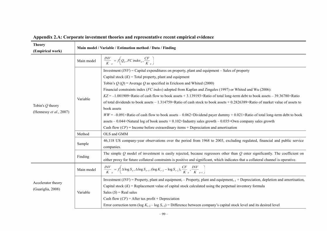
– 99 –
Appendix 2.A: Corporate investment theories and representative recent empirical evidence Theory (Empirical work)
Main model / Variable / Estimation method / Data / Finding
Tobin's Q theory (Hennessy et al., 2007)
Main model
ititit
it KCFindexFCQf
KINV , ,
Variable
Investment (INV) = Capital expenditures on property, plant and equipment – Sales of property Capital stock (K) = Total property, plant and equipment Tobin’s Q (Q) = Average Q as specified in Erickson and Whited (2000) Financial constraints index (FC index) adopted from Kaplan and Zingales (1997) or Whited and Wu (2006): KZ = –1.001909×Ratio of cash flow to book assets + 3.139193×Ratio of total long-term debt to book assets – 39.36780×Ratio of total dividends to book assets – 1.314759×Ratio of cash stock to book assets + 0.2826389×Ratio of market value of assets to book assets WW = –0.091×Ratio of cash flow to book assets – 0.062×Dividend payer dummy + 0.021×Ratio of total long-term debt to book assets – 0.044×Natural log of book assets + 0.102×Industry sales growth – 0.035×Own company sales growth Cash flow (CF) = Income before extraordinary items + Depreciation and amortisation
Method OLS and GMM
Sample 46,118 US company-year observations over the period from 1968 to 2003, excluding regulated, financial and public service companies.
Finding The simple Q model of investment is easily rejected, because regressors other than Q enter significantly. The coefficient on either proxy for future collateral constraints is positive and significant, which indicates that a collateral channel is operative.
Accelerator theory (Guariglia, 2008)
Main model
1221 , ),log(log ,log ,log
ititttitit
it KINV
KCFSKSSf
KINV
Variable
Investment (INV) = Property, plant and equipmentt – Property, plant and equipmentt–1 + Depreciation, depletion and amortisationt Capital stock (K) = Replacement value of capital stock calculated using the perpetual inventory formula Sales (S) = Real sales Cash flow (CF) = After tax profit + Depreciation Error correction term (log Kt–2 – log St–2) = Difference between company’s capital stock level and its desired level
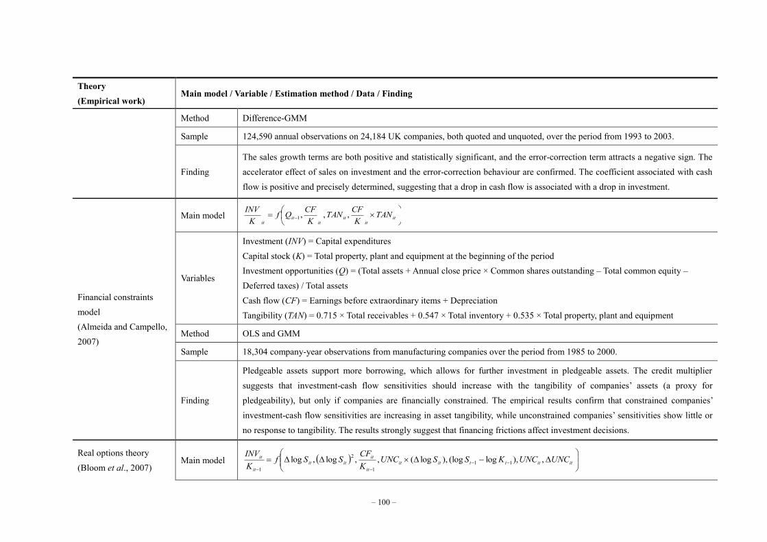
– 100 –
Theory (Empirical work)
Main model / Variable / Estimation method / Data / Finding
Method Difference-GMM
Sample 124,590 annual observations on 24,184 UK companies, both quoted and unquoted, over the period from 1993 to 2003.
Finding The sales growth terms are both positive and statistically significant, and the error-correction term attracts a negative sign. The accelerator effect of sales on investment and the error-correction behaviour are confirmed. The coefficient associated with cash flow is positive and precisely determined, suggesting that a drop in cash flow is associated with a drop in investment.
Financial constraints model (Almeida and Campello, 2007)
Main model
it
itit
itit
itTAN
KCFTAN
KCFQf
KINV , , ,1
Variables
Investment (INV) = Capital expenditures Capital stock (K) = Total property, plant and equipment at the beginning of the period Investment opportunities (Q) = (Total assets + Annual close price × Common shares outstanding – Total common equity – Deferred taxes) / Total assets Cash flow (CF) = Earnings before extraordinary items + Depreciation Tangibility (TAN) = 0.715 × Total receivables + 0.547 × Total inventory + 0.535 × Total property, plant and equipment
Method OLS and GMM
Sample 18,304 company-year observations from manufacturing companies over the period from 1985 to 2000.
Finding
Pledgeable assets support more borrowing, which allows for further investment in pledgeable assets. The credit multiplier suggests that investment-cash flow sensitivities should increase with the tangibility of companies’ assets (a proxy for pledgeability), but only if companies are financially constrained. The empirical results confirm that constrained companies’ investment-cash flow sensitivities are increasing in asset tangibility, while unconstrained companies’ sensitivities show little or no response to tangibility. The results strongly suggest that financing frictions affect investment decisions.
Real options theory (Bloom et al., 2007)
Main model
ititttititit
ititit
it
it UNCUNCKSSUNCKCF
SSfKINV
, ),log(log ),log( , ,log ,log 111
2
1
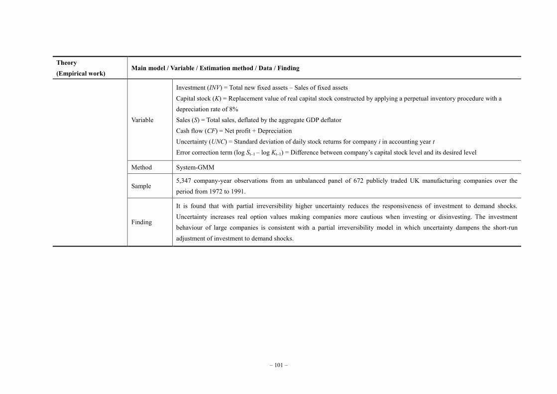
– 101 –
Theory (Empirical work)
Main model / Variable / Estimation method / Data / Finding
Variable
Investment (INV) = Total new fixed assets – Sales of fixed assets Capital stock (K) = Replacement value of real capital stock constructed by applying a perpetual inventory procedure with a depreciation rate of 8% Sales (S) = Total sales, deflated by the aggregate GDP deflator Cash flow (CF) = Net profit + Depreciation Uncertainty (UNC) = Standard deviation of daily stock returns for company i in accounting year t Error correction term (log St–1 – log Kt–1) = Difference between company’s capital stock level and its desired level
Method System-GMM
Sample 5,347 company-year observations from an unbalanced panel of 672 publicly traded UK manufacturing companies over the period from 1972 to 1991.
Finding
It is found that with partial irreversibility higher uncertainty reduces the responsiveness of investment to demand shocks. Uncertainty increases real option values making companies more cautious when investing or disinvesting. The investment behaviour of large companies is consistent with a partial irreversibility model in which uncertainty dampens the short-run adjustment of investment to demand shocks.
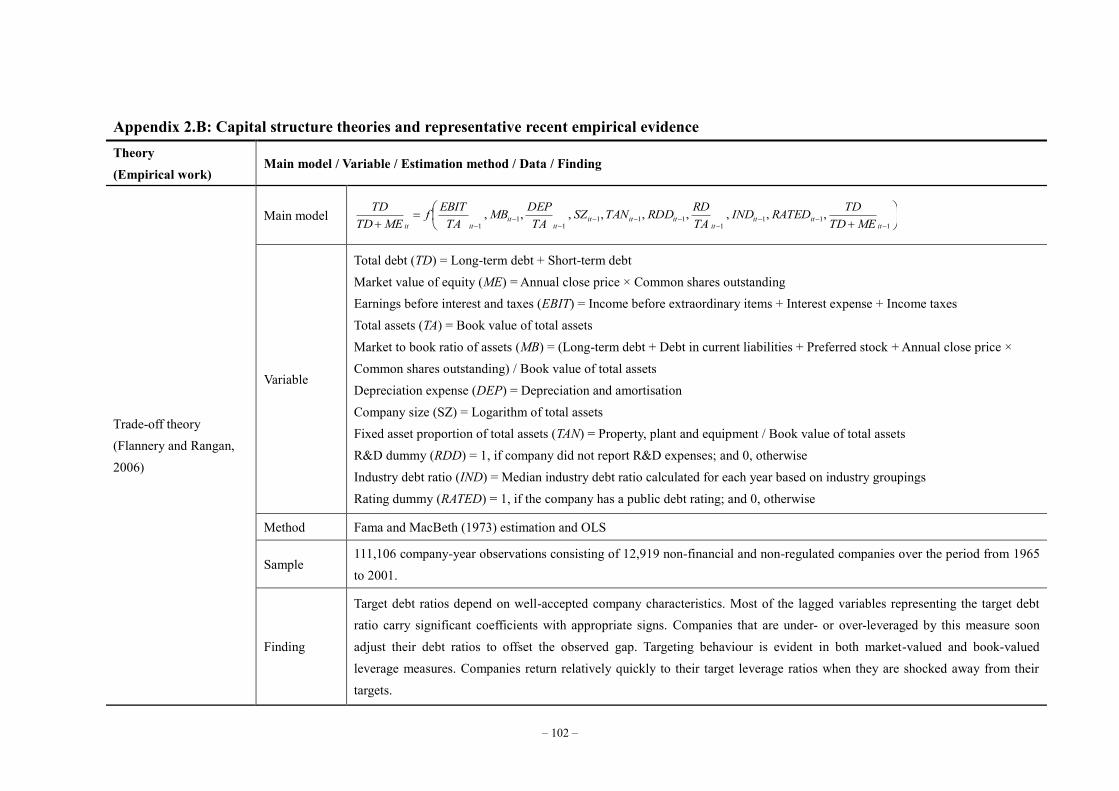
– 102 –
Appendix 2.B: Capital structure theories and representative recent empirical evidence Theory (Empirical work)
Main model / Variable / Estimation method / Data / Finding
Trade-off theory (Flannery and Rangan, 2006)
Main model
111
1111
11
1 , , , , , , , , ,
ititit
itititit
itit
itit METDTDRATEDIND
TARDRDDTANSZ
TADEPMB
TAEBITf
METDTD
Variable
Total debt (TD) = Long-term debt + Short-term debt Market value of equity (ME) = Annual close price × Common shares outstanding Earnings before interest and taxes (EBIT) = Income before extraordinary items + Interest expense + Income taxes Total assets (TA) = Book value of total assets Market to book ratio of assets (MB) = (Long-term debt + Debt in current liabilities + Preferred stock + Annual close price × Common shares outstanding) / Book value of total assets Depreciation expense (DEP) = Depreciation and amortisation Company size (SZ) = Logarithm of total assets Fixed asset proportion of total assets (TAN) = Property, plant and equipment / Book value of total assets R&D dummy (RDD) = 1, if company did not report R&D expenses; and 0, otherwise Industry debt ratio (IND) = Median industry debt ratio calculated for each year based on industry groupings Rating dummy (RATED) = 1, if the company has a public debt rating; and 0, otherwise
Method Fama and MacBeth (1973) estimation and OLS
Sample 111,106 company-year observations consisting of 12,919 non-financial and non-regulated companies over the period from 1965 to 2001.
Finding
Target debt ratios depend on well-accepted company characteristics. Most of the lagged variables representing the target debt ratio carry significant coefficients with appropriate signs. Companies that are under- or over-leveraged by this measure soon adjust their debt ratios to offset the observed gap. Targeting behaviour is evident in both market-valued and book-valued leverage measures. Companies return relatively quickly to their target leverage ratios when they are shocked away from their targets.
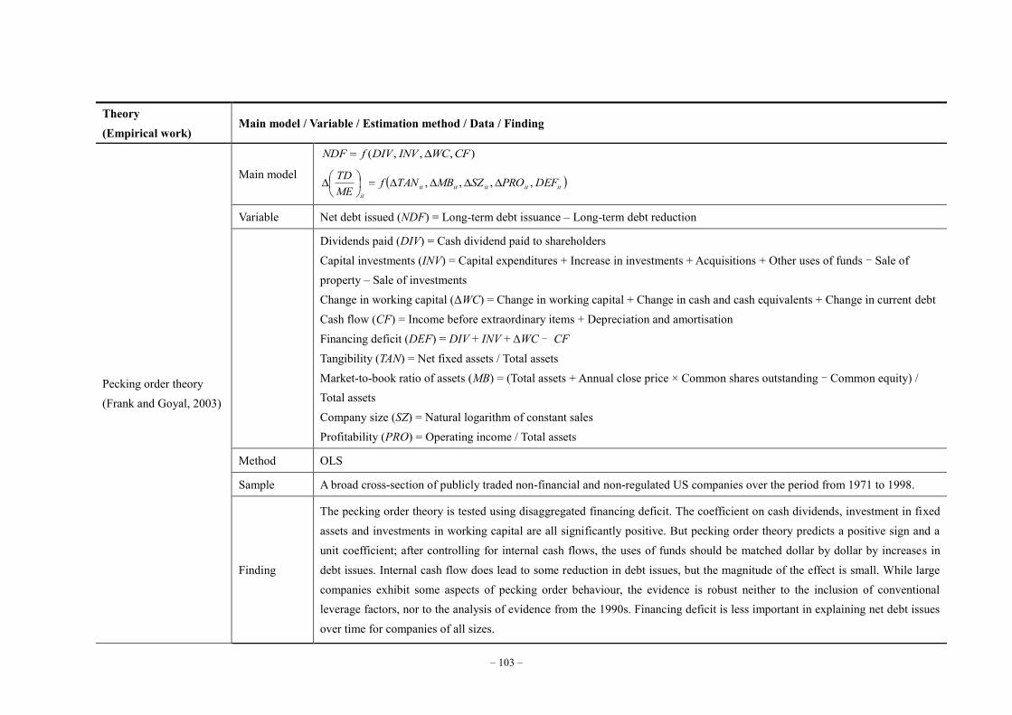
– 103 –
Theory (Empirical work)
Main model / Variable / Estimation method / Data / Finding
Pecking order theory (Frank and Goyal, 2003)
Main model
) , , ,( CFWCINVDIVfNDF
itititititit
DEFPROSZMBTANfMETD , , , ,
Variable Net debt issued (NDF) = Long-term debt issuance – Long-term debt reduction
Dividends paid (DIV) = Cash dividend paid to shareholders Capital investments (INV) = Capital expenditures + Increase in investments + Acquisitions + Other uses of funds - Sale of property – Sale of investments Change in working capital (ΔWC) = Change in working capital + Change in cash and cash equivalents + Change in current debt Cash flow (CF) = Income before extraordinary items + Depreciation and amortisation Financing deficit (DEF) = DIV + INV + ΔWC - CF Tangibility (TAN) = Net fixed assets / Total assets Market-to-book ratio of assets (MB) = (Total assets + Annual close price × Common shares outstanding - Common equity) / Total assets Company size (SZ) = Natural logarithm of constant sales Profitability (PRO) = Operating income / Total assets
Method OLS
Sample A broad cross-section of publicly traded non-financial and non-regulated US companies over the period from 1971 to 1998.
Finding
The pecking order theory is tested using disaggregated financing deficit. The coefficient on cash dividends, investment in fixed assets and investments in working capital are all significantly positive. But pecking order theory predicts a positive sign and a unit coefficient; after controlling for internal cash flows, the uses of funds should be matched dollar by dollar by increases in debt issues. Internal cash flow does lead to some reduction in debt issues, but the magnitude of the effect is small. While large companies exhibit some aspects of pecking order behaviour, the evidence is robust neither to the inclusion of conventional leverage factors, nor to the analysis of evidence from the 1990s. Financing deficit is less important in explaining net debt issues over time for companies of all sizes.
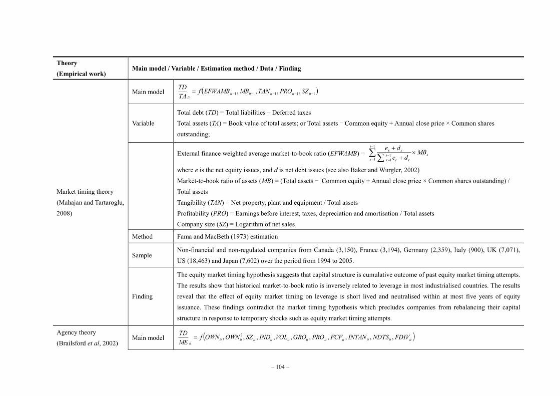
– 104 –
Theory (Empirical work)
Main model / Variable / Estimation method / Data / Finding
Market timing theory (Mahajan and Tartaroglu, 2008)
Main model 11111 , , , , itititititit
SZPROTANMBEFWAMBfTATD
Variable Total debt (TD) = Total liabilities – Deferred taxes Total assets (TA) = Book value of total assets; or Total assets - Common equity + Annual close price × Common shares outstanding;
External finance weighted average market-to-book ratio (EFWAMB) =
1
111
t
ss
rrtr
ss MBde
de
where e is the net equity issues, and d is net debt issues (see also Baker and Wurgler, 2002) Market-to-book ratio of assets (MB) = (Total assets - Common equity + Annual close price × Common shares outstanding) / Total assets Tangibility (TAN) = Net property, plant and equipment / Total assets Profitability (PRO) = Earnings before interest, taxes, depreciation and amortisation / Total assets Company size (SZ) = Logarithm of net sales
Method Fama and MacBeth (1973) estimation
Sample Non-financial and non-regulated companies from Canada (3,150), France (3,194), Germany (2,359), Italy (900), UK (7,071), US (18,463) and Japan (7,602) over the period from 1994 to 2005.
Finding
The equity market timing hypothesis suggests that capital structure is cumulative outcome of past equity market timing attempts. The results show that historical market-to-book ratio is inversely related to leverage in most industrialised countries. The results reveal that the effect of equity market timing on leverage is short lived and neutralised within at most five years of equity issuance. These findings contradict the market timing hypothesis which precludes companies from rebalancing their capital structure in response to temporary shocks such as equity market timing attempts.
Agency theory (Brailsford et al, 2002)
Main model itititititititititititit
FDIVNDTSINTANFCFPROGROVOLINDSZOWNOWNfMETD , , , , , , , , , , 2
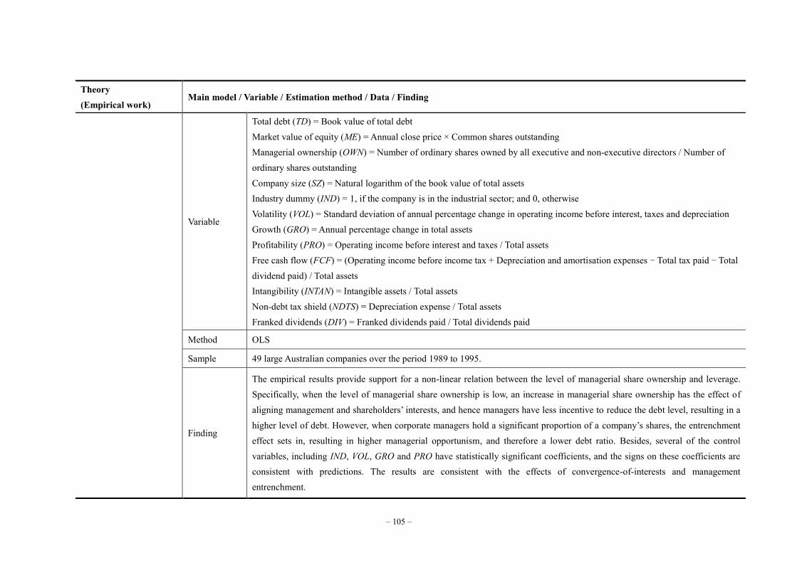
– 105 –
Theory (Empirical work)
Main model / Variable / Estimation method / Data / Finding
Variable
Total debt (TD) = Book value of total debt Market value of equity (ME) = Annual close price × Common shares outstanding Managerial ownership (OWN) = Number of ordinary shares owned by all executive and non-executive directors / Number of ordinary shares outstanding Company size (SZ) = Natural logarithm of the book value of total assets Industry dummy (IND) = 1, if the company is in the industrial sector; and 0, otherwise Volatility (VOL) = Standard deviation of annual percentage change in operating income before interest, taxes and depreciation Growth (GRO) = Annual percentage change in total assets Profitability (PRO) = Operating income before interest and taxes / Total assets Free cash flow (FCF) = (Operating income before income tax + Depreciation and amortisation expenses - Total tax paid - Total dividend paid) / Total assets Intangibility (INTAN) = Intangible assets / Total assets Non-debt tax shield (NDTS) = Depreciation expense / Total assets Franked dividends (DIV) = Franked dividends paid / Total dividends paid
Method OLS
Sample 49 large Australian companies over the period 1989 to 1995.
Finding
The empirical results provide support for a non-linear relation between the level of managerial share ownership and leverage. Specifically, when the level of managerial share ownership is low, an increase in managerial share ownership has the effect of aligning management and shareholders’ interests, and hence managers have less incentive to reduce the debt level, resulting in a higher level of debt. However, when corporate managers hold a significant proportion of a company’s shares, the entrenchment effect sets in, resulting in higher managerial opportunism, and therefore a lower debt ratio. Besides, several of the control variables, including IND, VOL, GRO and PRO have statistically significant coefficients, and the signs on these coefficients are consistent with predictions. The results are consistent with the effects of convergence-of-interests and management entrenchment.
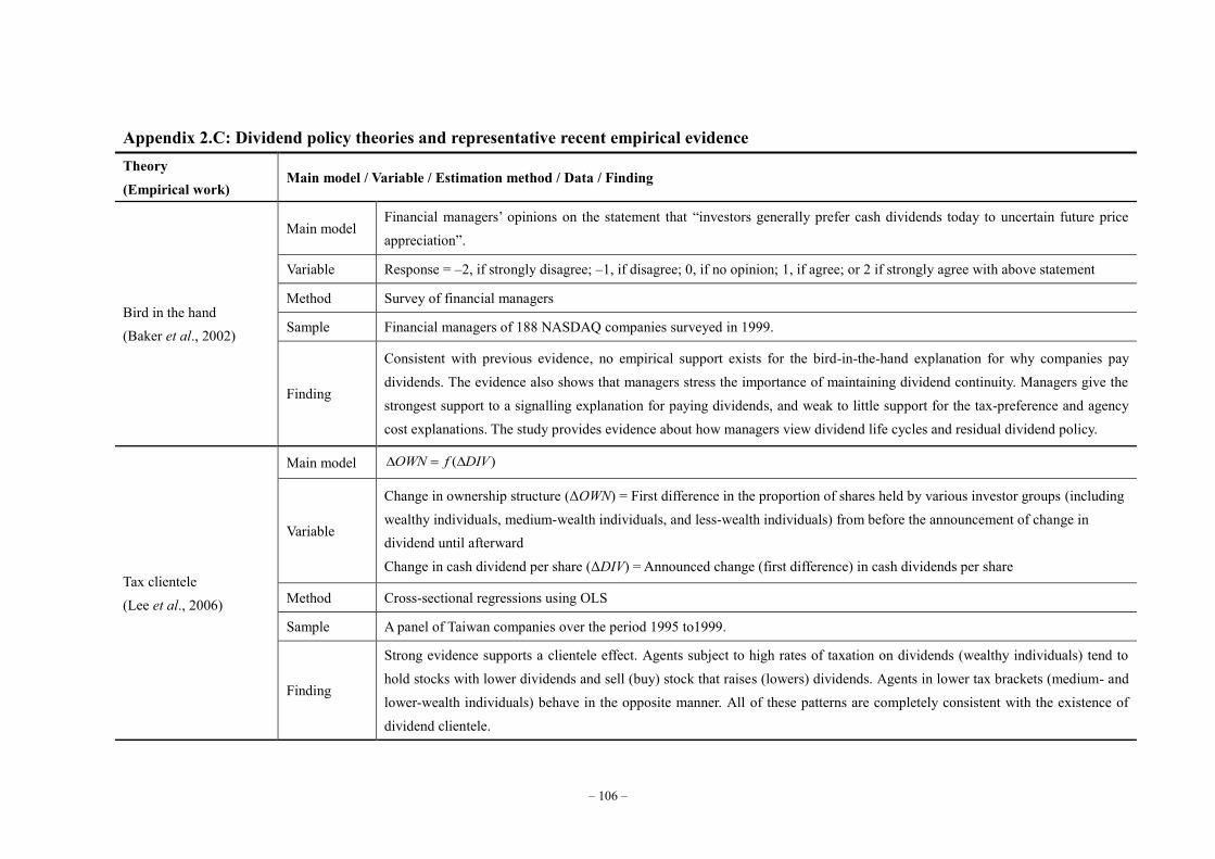
– 106 –
Appendix 2.C: Dividend policy theories and representative recent empirical evidence Theory (Empirical work)
Main model / Variable / Estimation method / Data / Finding
Bird in the hand (Baker et al., 2002)
Main model Financial managers’ opinions on the statement that “investors generally prefer cash dividends today to uncertain future price appreciation”.
Variable Response = –2, if strongly disagree; –1, if disagree; 0, if no opinion; 1, if agree; or 2 if strongly agree with above statement
Method Survey of financial managers
Sample Financial managers of 188 NASDAQ companies surveyed in 1999.
Finding
Consistent with previous evidence, no empirical support exists for the bird-in-the-hand explanation for why companies pay dividends. The evidence also shows that managers stress the importance of maintaining dividend continuity. Managers give the strongest support to a signalling explanation for paying dividends, and weak to little support for the tax-preference and agency cost explanations. The study provides evidence about how managers view dividend life cycles and residual dividend policy.
Tax clientele (Lee et al., 2006)
Main model )( DIVfOWN
Variable
Change in ownership structure (ΔOWN) = First difference in the proportion of shares held by various investor groups (including wealthy individuals, medium-wealth individuals, and less-wealth individuals) from before the announcement of change in dividend until afterward Change in cash dividend per share (ΔDIV) = Announced change (first difference) in cash dividends per share
Method Cross-sectional regressions using OLS
Sample A panel of Taiwan companies over the period 1995 to1999.
Finding
Strong evidence supports a clientele effect. Agents subject to high rates of taxation on dividends (wealthy individuals) tend to hold stocks with lower dividends and sell (buy) stock that raises (lowers) dividends. Agents in lower tax brackets (medium- and lower-wealth individuals) behave in the opposite manner. All of these patterns are completely consistent with the existence of dividend clientele.
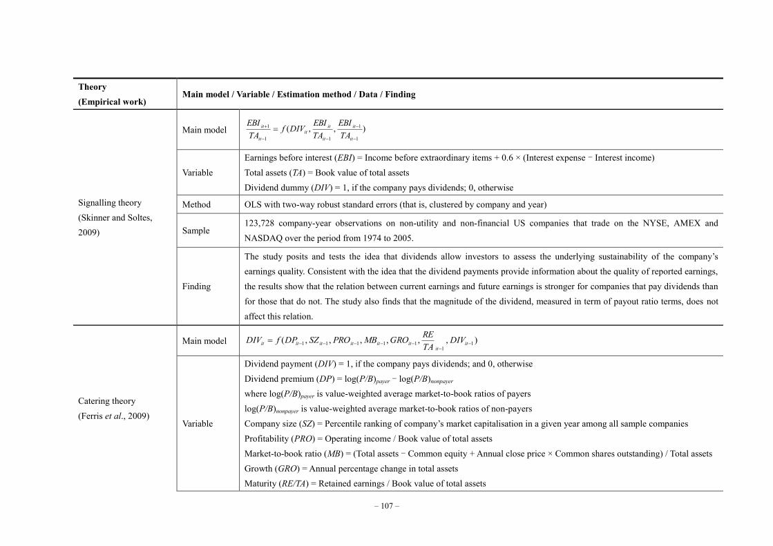
– 107 –
Theory (Empirical work)
Main model / Variable / Estimation method / Data / Finding
Signalling theory (Skinner and Soltes, 2009)
Main model ) , ,(1
1
11
1
it
it
it
itit
it
it
TAEBI
TAEBI
DIVfTAEBI
Variable Earnings before interest (EBI) = Income before extraordinary items + 0.6 × (Interest expense - Interest income) Total assets (TA) = Book value of total assets Dividend dummy (DIV) = 1, if the company pays dividends; 0, otherwise
Method OLS with two-way robust standard errors (that is, clustered by company and year)
Sample 123,728 company-year observations on non-utility and non-financial US companies that trade on the NYSE, AMEX and NASDAQ over the period from 1974 to 2005.
Finding
The study posits and tests the idea that dividends allow investors to assess the underlying sustainability of the company’s earnings quality. Consistent with the idea that the dividend payments provide information about the quality of reported earnings, the results show that the relation between current earnings and future earnings is stronger for companies that pay dividends than for those that do not. The study also finds that the magnitude of the dividend, measured in term of payout ratio terms, does not affect this relation.
Catering theory (Ferris et al., 2009)
Main model ) , , , , , ,( 11
11111
itit
itititititit DIVTAREGROMBPROSZDPfDIV
Variable
Dividend payment (DIV) = 1, if the company pays dividends; and 0, otherwise Dividend premium (DP) = log(P/B)payer - log(P/B)nonpayer where log(P/B)payer is value-weighted average market-to-book ratios of payers log(P/B)nonpayer is value-weighted average market-to-book ratios of non-payers Company size (SZ) = Percentile ranking of company’s market capitalisation in a given year among all sample companies Profitability (PRO) = Operating income / Book value of total assets Market-to-book ratio (MB) = (Total assets - Common equity + Annual close price × Common shares outstanding) / Total assets Growth (GRO) = Annual percentage change in total assets Maturity (RE/TA) = Retained earnings / Book value of total assets
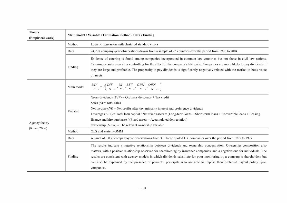
– 108 –
Theory (Empirical work)
Main model / Variable / Estimation method / Data / Finding
Method Logistic regression with clustered standard errors
Data 24,298 company-year observations drawn from a sample of 23 countries over the period from 1996 to 2004.
Finding
Evidence of catering is found among companies incorporated in common law countries but not those in civil law nations. Catering persists even after controlling for the effect of the company’s life cycle. Companies are more likely to pay dividends if they are large and profitable. The propensity to pay dividends is significantly negatively related with the market-to-book value of assets.
Agency theory (Khan, 2006)
Main model
11 , , , ,
itititititit SOWN
SOWN
SLEV
SNI
SDIVf
SDIV
Variable
Gross dividends (DIV) = Ordinary dividends + Tax credit Sales (S) = Total sales Net income (NI) = Net profits after tax, minority interest and preference dividends Leverage (LEV) = Total loan capital / Net fixed assets = (Long-term loans + Short-term loans + Convertible loans + Leasing finance and hire purchase) / (Fixed assets – Accumulated depreciation) Ownership (OWN) = The relevant ownership variable
Method OLS and system-GMM
Data A panel of 3,030 company-year observations from 330 large quoted UK companies over the period from 1985 to 1997.
Finding
The results indicate a negative relationship between dividends and ownership concentration. Ownership composition also matters, with a positive relationship observed for shareholding by insurance companies, and a negative one for individuals. The results are consistent with agency models in which dividends substitute for poor monitoring by a company’s shareholders but can also be explained by the presence of powerful principals who are able to impose their preferred payout policy upon companies.
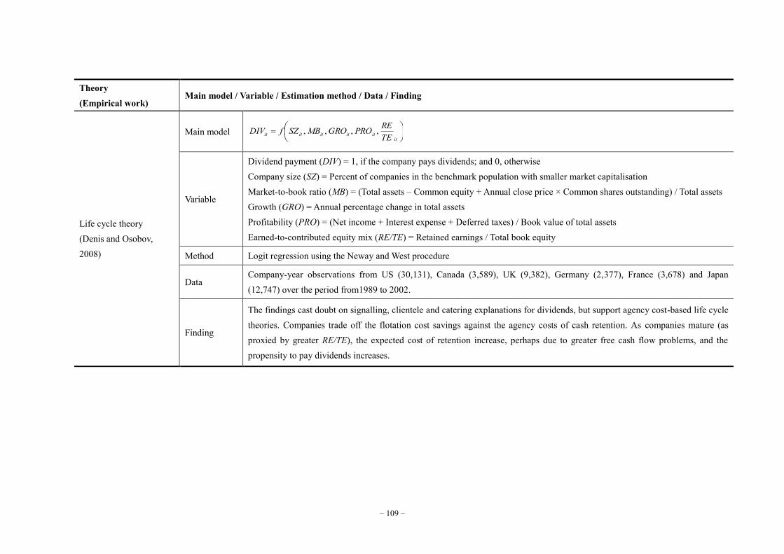
– 109 –
Theory (Empirical work)
Main model / Variable / Estimation method / Data / Finding
Life cycle theory (Denis and Osobov, 2008)
Main model
itititititit TE
REPROGROMBSZfDIV , , , ,
Variable
Dividend payment (DIV) = 1, if the company pays dividends; and 0, otherwise Company size (SZ) = Percent of companies in the benchmark population with smaller market capitalisation Market-to-book ratio (MB) = (Total assets – Common equity + Annual close price × Common shares outstanding) / Total assets Growth (GRO) = Annual percentage change in total assets Profitability (PRO) = (Net income + Interest expense + Deferred taxes) / Book value of total assets Earned-to-contributed equity mix (RE/TE) = Retained earnings / Total book equity
Method Logit regression using the Neway and West procedure
Data Company-year observations from US (30,131), Canada (3,589), UK (9,382), Germany (2,377), France (3,678) and Japan (12,747) over the period from1989 to 2002.
Finding
The findings cast doubt on signalling, clientele and catering explanations for dividends, but support agency cost-based life cycle theories. Companies trade off the flotation cost savings against the agency costs of cash retention. As companies mature (as proxied by greater RE/TE), the expected cost of retention increase, perhaps due to greater free cash flow problems, and the propensity to pay dividends increases.
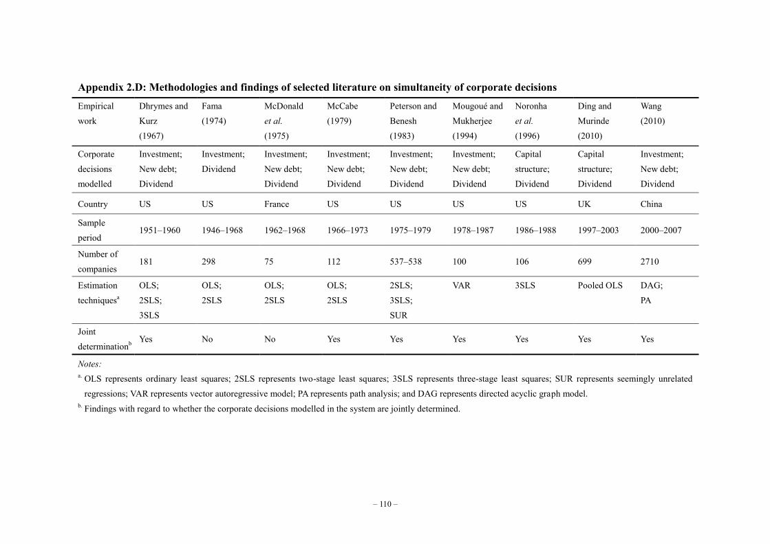
– 110 –
Appendix 2.D: Methodologies and findings of selected literature on simultaneity of corporate decisions
Empirical work
Dhrymes and Kurz (1967)
Fama (1974)
McDonald et al. (1975)
McCabe (1979)
Peterson and Benesh (1983)
Mougoué and Mukherjee (1994)
Noronha et al. (1996)
Ding and Murinde (2010)
Wang (2010)
Corporate decisions modelled
Investment; New debt; Dividend
Investment; Dividend
Investment; New debt; Dividend
Investment; New debt; Dividend
Investment; New debt; Dividend
Investment; New debt; Dividend
Capital structure; Dividend
Capital structure; Dividend
Investment; New debt; Dividend
Country US US France US US US US UK China
Sample period
1951–1960 1946–1968 1962–1968 1966–1973 1975–1979 1978–1987 1986–1988 1997–2003 2000–2007
Number of companies
181 298 75 112 537–538 100 106 699 2710
Estimation techniquesa
OLS; 2SLS; 3SLS
OLS; 2SLS
OLS; 2SLS
OLS; 2SLS
2SLS; 3SLS; SUR
VAR 3SLS Pooled OLS DAG; PA
Joint determinationb
Yes No No Yes Yes Yes Yes Yes Yes
Notes: a. OLS represents ordinary least squares; 2SLS represents two-stage least squares; 3SLS represents three-stage least squares; SUR represents seemingly unrelated
regressions; VAR represents vector autoregressive model; PA represents path analysis; and DAG represents directed acyclic graph model. b. Findings with regard to whether the corporate decisions modelled in the system are jointly determined.

Chapter 3: Corporate Decisions, Financial Constraints and Uncertainty
– 111 –
CHAPTER 3
CORPORATE DECISIONS, FINANCIAL CONSTRAINTS
AND UNCERTAINTY
3.1 Introduction
Corporations face investment, financing and payout choices which are known as the trilogy of
corporate decisions (Wang, 2010). Although much effort has been devoted to investigating
this key set of corporate decisions in the literature, they have typically been treated separately,
and hence there has been little analysis of the simultaneity among them. A review of the
conventional wisdom on the three aspects of corporate behaviour is provided in Section 2.2,
but nothing at all about the interactions that may exist among them.
Chapter 2 of this thesis provides a comprehensive review of relevant literature. Suffice
it to point out here that prior research has provided reasons and evidence that financial
constraints, such as limited availability of internal finance and access to new external finance,
may hamper companies’ ability to invest efficiently (see the literature reviewed in Section 2.3).
According to this view, companies should consider their fund-raising choices alongside their
fund-spending decisions. An important implication is that corporate investment, financing and
payout decisions are likely to be interdependent upon one another and jointly determined by
management. Nevertheless, previous studies that empirically investigate companies’ real and
financial decisions overwhelmingly employ single equation techniques, and thus permit no

Chapter 3: Corporate Decisions, Financial Constraints and Uncertainty
– 112 –
analysis of the contemporaneous interactions among these corporate decisions, leading to
incomplete view of corporate behaviour (Gatchev et al., 2010). To overcome the shortcoming
of single equation techniques, this chapter highlights the potential joint determination of
corporate investment, financing and payout decisions by modelling them within a
simultaneous system which explicitly allows for the interactions among them. The
simultaneity analysis may reveal new insights into the inter-relationships that may exist
among the set of corporate decisions, improving our knowledge of the complex corporate
decision-making processes.
The set of corporate decisions are potentially interdependent not only because they
may affect one another directly, but also because they are likely to be affected by substantially
overlapping information. As discussed in Section 2.4, recent literature that seeks to explore
the determinants of corporate investment behaviour has highlighted the importance of
uncertainty associated with companies’ prospects. However, the role that uncertainty plays in
financing and payout decisions has received little attention. Due to the fact that all corporate
decisions are made on the basis of uncertain information, it is plausible to argue that the
degree of uncertainty matters in both financing and payout decisions as well. If this is true,
uncertainty may not only influence corporate investment decisions directly on its own, but
also indirectly through its effects on financing and payout choices. The omission of relevant
information in modelling corporate decisions is likely to generate misleading results and lead
to inappropriate inferences, which may bias our understanding of corporate behaviour.
Chapter 3: Corporate Decisions, Financial Constraints and Uncertainty
– 113 –
Therefore, this chapter seeks to fill these gaps in the literature by considering uncertainty
associated with a company’s future prospects as a common factor that involved in each of the
decisions modelled in our simultaneous system, in an attempt to comprehensively investigate
corporate behaviour under uncertainty.
Based on a large panel of UK-listed companies within the period 1999–2008, this
chapter empirically investigates the interactions among corporate investment, financing and
payout decisions in the presence of financial constraints and uncertainty, contributing to the
current knowledge of corporate behaviour in a number of ways. First, we develop a
simultaneous equations system that explicitly accounts for the interactions among the three
corporate decisions, with each of the decision variables being treated as endogenous and
being subject to the constraint that sources must equal uses of funds, as implied by the
flow-of-funds framework. The simultaneous equations analysis, therefore, overcomes the
shortcomings of single equation techniques that are currently adopted in the existing literature,
and provides new insights into the interdependences among corporate decisions in the real
world. Second, we include the degree of uncertainty associated with a company’s prospects as
an explanatory variable in each of the decisions equations modelled in our simultaneous
system. By including an uncertainty variable into the simultaneous system, we explicitly
allow uncertainty to not only affect each of the corporate decisions directly on its own, but
also indirectly through its effect on other corporate decisions. Such analyses can provide us
better knowledge of corporate decision-making behaviour under uncertain circumstances.

Chapter 3: Corporate Decisions, Financial Constraints and Uncertainty
– 114 –
Third, we explicitly explore the possible mechanisms through which the set of corporate
decisions are determined simultaneously, by splitting the whole sample into two with
financially more constrained and financially less constrained companies, based on a financial
leverage index. We believe that our exclusive research design can shed light and provide a
deeper understanding on corporate decision-making behaviour in the real world.
The remainder of this chapter is organised as follows. Section 3.2 reviews the
empirical measures of uncertainty used in the existing literature. Section 3.3 develops a
theoretical framework. Section 3.4 specifies the corporate behavioural equations. Section 3.5
discusses the sample, variables and preliminary analysis. Section 3.6 describes the estimation
and testing procedures as well as the main results for the empirical models. Section 3.7 offers
further evidence to check the robustness of our findings. Concluding remarks are drawn in
Section 3.8.
3.2 Empirical proxies for uncertainty
The primary challenges of establishing the relations between uncertainty and corporate
decisions are to identify the sources and to quantify the levels of uncertainty associated with
companies’ future prospects (Carruth et al., 2000). There is a considerable debate regarding
how uncertainty should be captured empirically. To date, no consensus has been reached
about the best practice of measuring uncertainty in empirical analyses. A number of broad
approaches have been employed in the existing literature to construct proxy measures for
uncertainty, but none of them appears without its particular problems and criticisms. This
Chapter 3: Corporate Decisions, Financial Constraints and Uncertainty
– 115 –
section, therefore, summarises the most commonly used empirical measures of uncertainty in
the existing literature, which may provide us with guidance in formulating proxy measures for
uncertainty.
3.2.1 Output volatility
Output volatility measures the variation in the expected revenue from an investment project.
In the empirical literature, output volatility is typically defined as the variations in product
price, product demand or total sales, which can be considered as consequences of
demand-side shocks. According to the neoclassical investment model, a company’s profit is a
convex function with respect to the output price. Increased output volatility, therefore, raises
the expected present value of future profit and encourages the company to undertake
investment opportunities (see, for example, Hartman, 1972; and Abel, 1983).
Henley et al. (2003) measure industry-wide product price uncertainty using a moving
standard deviation of the producer price index of the corresponding sector. However, the use
of historical volatility has been widely criticised for being backward looking and failing to
carry uncertainty information for future periods. In an attempt to devise a better proxy for
uncertainty, Ghosal and Loungani (1996) assume that companies attempt to forecast their
product prices using an autoregressive (AR) model. They argue that the unpredictable part of
the stochastic process can be used to formulate a more reasonable measure that captures
output price shocks. Accordingly, they calculate a rolling standard error of the forecasting
residuals, and use it as the proxy for output price uncertainty. The major problem of using
Chapter 3: Corporate Decisions, Financial Constraints and Uncertainty
– 116 –
product price volatility to measure uncertainty is that the price indices are normally only
available at aggregate levels, and thus are unlikely to carry uncertainty information specific to
individual companies.
Guiso and Parigi (1999) employ product demand volatility to proxy for the output
uncertainty. They draw information about managerial perception of future demand for their
products from a survey conducted by the Bank of Italy. The conditional mean and variance
derived from the survey data are used to measure the expected level of product demand and
the expected degree of demand uncertainty, respectively. These measures, based on the
managers’ subjective certainty about their expectations, are expected to be more closely
related to the investment decisions made by individual companies under different
circumstances. In much the same vein, Calcagnini and Saltari (2001) also derive a proxy for
uncertainty from business survey results regarding expected growth in demand, and use it to
analyse the relationship between investment and demand uncertainty at aggregate level.
However, due to the limited availability of survey data, the use of survey-based demand
uncertainty proxies is relatively rare in the existing literature.
The most commonly used output uncertainty proxy is based on the volatility of
companies’ total sales. Because sales data can be easily obtained from a company’s income
statement, it enables empirical studies to more accurately explore the effect of a company’s
idiosyncratic output uncertainty on its investment decisions by using company-specific
information. Lensink and Sterken (2000) measure companies’ output uncertainty using the
Chapter 3: Corporate Decisions, Financial Constraints and Uncertainty
– 117 –
standard deviation of historical total sales. To account for the size effect, the standard
deviation of total sales is scaled by its mean value to form the coefficient of variation of the
underlying variable. The use of proxy for uncertainty at disaggregate level can effectively deal
with the problems of heterogeneity across companies which may potentially bias the results
from studies at aggregate levels (Carruth et al., 2000).
3.2.2 Input volatility
Input volatility measures uncertainty with respect to the prices of labour, raw materials and
other on-going operating expenses that extend over time once a project is committed. Input
volatility measures are expected to capture the supply-side uncertainty.
By assuming a fixed capital-labour ratio for a given level of technology, Huizinga
(1993) considers the real wage as a proxy for the on-going operating expense. Accordingly, he
constructs a bivariate autoregressive conditional heteroscedasticity (ARCH) model to estimate
the conditional standard deviation of quarterly real wage, which is then used as a proxy for
uncertainty associated with input costs in a model of aggregate investment. Besides this,
Huizinga (1993) constructs another proxy for input uncertainty based on the volatility of
material prices. It is found that aggregate investment appears to be negatively associated with
both real wage and material price volatility. The results also indicate that any single volatility
measure at aggregate levels is unlikely to adequately capture the various dimensions of
uncertainty faced by a company. At disaggregate level, Lensink and Sterken (2000) use the
volatility of employee costs as one of the proxies for uncertainty to investigation investment
Chapter 3: Corporate Decisions, Financial Constraints and Uncertainty
– 118 –
behaviour of companies under uncertain circumstances. However, due to the limited time
period for company-level data, they simply measure uncertainty using the coefficient of
variation of the underlying variable.
3.2.3 Profit volatility
Profit variables take both sales and costs into consideration, and thus the variation in profit
counts for both input and output uncertainties. Therefore, profit volatility is typically regarded
as a more general and more plausible proxy for uncertainty that carries information more
relevant to an individual company’s corporate decisions.
The standard deviation of the unpredictable component of profit has been widely used
in empirical studies as a proxy for uncertainty. For example, Ghosal and Loungani (2000) set
up a basic autoregressive forecasting equation for profit variable, and measure uncertainty
using the standard deviation of the forecasting residuals. However, it is documented that the
main concern about proxies for uncertainty derived from the forecasting residuals is that they
are likely to be sensitive to the specification of the forecasting models (Carruth et al., 2000).
Therefore, it is important to carry out various specification tests to ensure that the forecasting
model is correctly specified and statistically adequate.
Bond and Cummins (2004) develop a more innovative approach to measure
uncertainty based on analysts’ profits forecasts. They argue that more disagreement among
different securities analysts is likely to be associated with greater underlying uncertainty
about a company’s future prospects. Accordingly, Bond and Cummins (2004) measure the
Chapter 3: Corporate Decisions, Financial Constraints and Uncertainty
– 119 –
dispersion across individual analysts’ earnings per share forecasts for each company, and use
it as a proxy for the company’s profit uncertainty in their empirical investigation into the
investment-uncertainty relationship. In addition, Bond and Cummins (2004) construct an
alternative proxy for profit uncertainty using the variance of analyst forecast error, by arguing
that large analyst forecast error is likely to reflect a high degree of uncertainty, and vice versa.
The main advantage of Bond and Cummins’ (2004) novel measures of uncertainty is that they
carry information directly related to agents’ expectation on companies’ future profitability.
However, the sample size is limited by the number of companies with sufficient analyst
following.
3.2.4 Stock returns volatility
Stock returns volatility measures the variation of the changes in a company’s share price. If
the market is efficient, all information about a company’s asset fundamentals and growth
opportunities should be properly translated into its share price. Thus, the volatility of a
company’s stock returns is expected to summarise the volatilities of all aspects of the
company’s future prospects, capturing the overall uncertainty relevant to the company’s
investment decisions. This approach is adopted by most recent empirical studies to construct
forward looking uncertainty measures, and the difference mainly lies in the statistics used to
measure the volatility.
The standard deviation of stock returns is the most commonly used statistic to measure
uncertainty. For example, Bond and Cummins (2004) and Lensink and Murinde (2006)
Chapter 3: Corporate Decisions, Financial Constraints and Uncertainty
– 120 –
simply quantify the degree of uncertainty faced by a company using the standard deviation of
its daily stock returns observed over the period. A similar methodology is employed in Bulan
(2005), where the standard deviation of daily stock returns is annualised to match the financial
variables, which are only available on a yearly basis. However, there is a growing body of
evidence suggests that the use of more sophisticated time series models can lead to better
predictions of future volatility.
Since the stock market data are reported at a sufficient high frequency, it facilitates the
application of the generalised autoregressive conditional heteroscedasticity (GARCH)-type
modelling of volatility, which is able to generate more precise estimates of future uncertainty.
To take the advantage of the high-frequency stock market information, Lensink and Murinde
(2006) set up an autoregressive model to estimate the conditional mean of the stock returns,
and simultaneously specify a GARCH model to estimate its conditional variance and thus
conditional standard deviation. The average of the estimated conditional standard deviations
over each period is then calculated for each company and used as a measure of the company’s
idiosyncratic uncertainty for the corresponding period. In order to account for the asymmetric
component embedded in the volatility of stock returns, Bo and Lensink (2005) specify both
threshold ARCH (TARCH) and exponential GARCH (EGARCH) models to derive volatility
measures. These extended GARCH-type model allow for the asymmetric response of stock
return volatility to positive and negative shocks. Specifically, negative shocks are allowed to
have more impact on future volatility than positive shocks are the same magnitude.

Chapter 3: Corporate Decisions, Financial Constraints and Uncertainty
– 121 –
Similar methodologies are also employed to measure aggregate uncertainty at industry
and market levels, for example, the standard deviation of monthly stock market returns is used
in Lensink (2002) as an uncertainty measure at aggregate level. Moreover, the use of
aggregate stock market series also provides a channel to decompose a company’s overall
uncertainty into its market, industry and company-specific components. Bulan (2005) uses the
volatility of daily stock returns as a proxy for the company’s overall uncertainty. Similarly, the
volatilities of daily returns on market index and industry index are considered as proxies for
total market uncertainty and total industry uncertainty, respectively. A recent study by Baum
et al. (2008) also utilises the intra-annual volatilities of daily stock returns and market index
returns to distinguish between intrinsic and extrinsic uncertainty.
However, the use of stock returns volatility as proxy for uncertainty can be criticised
from several aspects. The main concern with this approach is that share prices may be too
noisy to provide useful information, because the volatility in stock market returns is likely to
be driven not only by movements in company fundamentals but also by speculative bubbles.
Besides, there is also a criticism that, although stock market returns may contain certain
information about a company’s cash flow uncertainty, they may reveal rather less about
uncertainty associated with future economic shocks and policy changes, thus fail to capture
the overall uncertainty associated with the company’s future prospects (Carruth et al. 2000).
3.2.5 Macroeconomic volatility
Macroeconomic uncertainty is also considered by some empirical studies, especially those at
Chapter 3: Corporate Decisions, Financial Constraints and Uncertainty
– 122 –
aggregate levels. The volatilities of macroeconomic variables, such as GDP, interest rate,
inflation rate and exchange rate, are expected to have influence on the corporate decisions of a
large number of companies in an economy.
It is well documented that, since an economy faces more uncertainty in the distant
future than in the near term, longer maturity of bonds entails greater uncertainty for investors.
Under the assumption of risk aversion, the holders of long-term bonds, who are subject to
greater risk, must be compensated by a risk premium. Therefore, the risk premium embedded
in the term structure of interest rates facilitates the measuring of uncertainty associated with
the macro economy. Accordingly, Ferderer (1993) uses the expected excess holding period
return of long-term bonds over short-term bonds to estimate the risk premium. The implicit
risk premium embedded in the term structure of interest rate is then used as a proxy for the
uncertainty associated with interest rates and other macroeconomic variables.
Apart from the measure derived from the term structure of interest rate,
macroeconomic volatility is also typically estimated based on the variations in GDP, inflation
rate and exchange rate. For example, Price (1995) utilises a GARCH-in-mean (GARCH-M)
estimate of conditional variance of GDP as a proxy for macroeconomic uncertainty. However,
it is criticised that macroeconomic volatility measures are unlikely to adequately capture the
various dimensions of uncertainty faced by corporate decision makers, and thus fail to capture
all relevant uncertainty sources (Carruth et al., 2000).
As can be seen, there is no consensus about how uncertainty should be captured
Chapter 3: Corporate Decisions, Financial Constraints and Uncertainty
– 123 –
empirically. A number of broad approaches have been adopted in the existing literature to
formulate proxy measures of uncertainty, ranging from output volatility to input volatility and
from stock return volatility to macroeconomic volatility. Nevertheless, it is generally agreed
that corporate decisions tend to be more sensitive to company idiosyncratic uncertainty than
to macroeconomic uncertainty which affect all companies in general. Thus, uncertainty
measures at disaggregate levels should be better able to capture all relevant uncertainty
sources which may affect an individual company’s decisions. Meanwhile, it is also widely
believed that, compared with backward looking measures, forward looking measures reveal
more information about both the range and the magnitude of uncertainty facing corporate
decision makers (Carruth et al., 2000). Therefore, it is desirable to construct forward looking
measures of uncertainty at company level to investigate aspects of corporate behaviour under
uncertain circumstances.
3.3 An information asymmetry-based flow-of-funds framework for corporate behaviour
To justify the fundamental interactions among corporate investment, financing and payout
decisions, we derive a model from a company’s flow-of-funds identity, i.e. a company’s uses
of funds must equal its sources of funds. Based on stylised financial statements, a company’s
main sources and uses of funds identity can be expressed as follows,
DEPPROEQUSDLDDIVCAFA (3.1)
Chapter 3: Corporate Decisions, Financial Constraints and Uncertainty
– 124 –
where FA represents fixed assets, CA current assets, DIV dividends paid to shareholders, LD
long-term debt, SD short-term debt, EQU common and preferred stock (exclusive of retained
earnings), PRO net income after tax, DEP depreciation allowances, and ∆ the change in a
variable from t–1 to t. The flow-of-funds identity states that companies raise funds from
external debt (∆LD and ∆SD), external equity (∆EQU) as well as internally generated cash
flow (PRO and DEP), and spend it on investment in assets (∆FA and ∆CA) and dividend
payout (DIV). The overriding constraint presented in Equation 3.1 is that the uses of funds
must equal the sources of funds. If the capital markets are sufficiently imperfect, companies
have to consider the availability of internal and external funds alongside their investment and
payout decisions, such that the set of corporate decisions may be determined jointly and
should be viewed as a simultaneous and interdependent process. The flow-of-funds identity
specified in Equation 3.1 can also be reparameterised into the following form,
DEPPROEQUSDNDFDIVCAINV (3.2)
where INV represents investment, i.e. the change in fixed assets over a period (∆FA), NDF
represents the net amount of new debt issued, i.e. the change in long-term debt outstanding
(∆LD). Among the various uses and sources of funds specified in Equation 3.2, the primary
focus of our model is on capital investment (INV), long-term debt financing (NDF) and
dividend payout (DIV) decisions. Internally generated cash flow (CF), which can be defined
Chapter 3: Corporate Decisions, Financial Constraints and Uncertainty
– 125 –
as the sum of net income (PRO) and non-cash expenses (DEP), is assumed to be determined
by past investment and financing decisions.13 Following the tradition of the corporate finance
literature, we treat internally generated cash flow as exogenous or predetermined in our model.
Moreover, it is argued that the changes in the elements contained in current assets (CA) and
short-term debts (SD), such as inventories, accounts receivable, and accounts payable, are
likely to be triggered by economic conditions, thus cannot be interpreted as the result of
conscious decisions made by managers (see, for example, Kadapakkam et al., 1998).
Accordingly, we treat the net changes in working capital (∆WC, which is equivalent to
SDCA ) as unintended residuals that balance the uses and sources of funds. Besides, in
the presence of information asymmetry, external equity financing (∆EQU) is rationally
viewed by investors as bad news that the stock is overpriced, thus managers are extremely
reluctant to issue new equity in the stock market for fear of sending a negative signal to the
markets. As a result, external equity financing is typically considered as a last resort and is
rarely used. Given the fact that external equity finance is a less significant source of funds for
listed companies after their initial public offerings, we drop ∆EQU from the flow-of-funds
framework for simplicity. 14 Therefore, the reduced form flow-of-funds identity can be
specified as follows,
13 It is believed that corporate decisions affect output (and profits) only with lags so that current corporate decisions affect only future output and hence profits, and that current output and current profits are not affected by current corporate decisions (see, for example, Dhrymes and Kurz, 1967; and McCabe, 1979). 14 Shyam-Sunder and Myers (1999) argue that, in the presence of asymmetric information, external equity financing is only used in extreme circumstances after initial public offering. Cleary et al. (2007) show that debt finance is the most significant source of external finance in all countries, and new equity finance accounts for only a very small proportion of total corporate financing.
Chapter 3: Corporate Decisions, Financial Constraints and Uncertainty
– 126 –
CFNDFWCDIVINV (3.3)
where INV, NDF and DIV are the three endogenous variables, representing investment outlays,
net long-term debt financing and dividend payout respectively; CF represents cash flow,
which is taken as exogenous; ∆WC represents the net change in working capital, which is
considered as the residual to balance company’s uses and sources of funds. Since the external
equity financing variable (∆EQU) is omitted in Equation 3.3, the reduced form flow-of-funds
identity is no longer an equality (=) but an approximation ( ). Given the arguments presented
above, the number of endogenous variables in the simultaneous equations system reduces to
three, namely, capital investment, long-term debt financing and dividend payout. Thus, the
empirical framework comprises estimation of the following simultaneous equations system,
) , , ,( ACFDIVNDFfINV (3.4)
) , , ,( BCFDIVINVfNDF (3.5)
) , , ,( CCFINVNDFfDIV (3.6)
where A, B and C are vectors of other exogenous variables which, according to existing
literature, are the stylised determinants of corporate investment, financing and payout
decisions, respectively. The three endogenous variables are the dependent variables for the
Chapter 3: Corporate Decisions, Financial Constraints and Uncertainty
– 127 –
corresponding equations. Each equation contains the two remaining endogenous variables as
explanatory variables, along with a predetermined cash flow variable and other exogenous
determinants. It is worth mentioning that, although the net changes in working capital (∆WC)
is considered as the residual to balance company’s uses and sources of funds, there is
nevertheless a behavioural relation implied for working capital by Equations 3.4–3.6 through
the adding-up restrictions implied by the reduced form flow-of-funds identity specified as
Equation 3.3. The implication for working capital, however, is beyond the scope of this study.
We hypothesise that, in the presence of information asymmetry, both internal and
external funds available for investment are likely to be constrained. To provide further
insights into the potential interactions among the set of corporate decisions, in particular the
influence of a company’s financial decisions on its real decisions, we appeal to the superior
knowledge that managers may possess about the company’s fundamentals and prospects.
Miller and Rock (1985) hypothesise that, in the presence of information asymmetry,
managers may use dividends as a signal to reveal some of their private information to the
markets. The signalling effect of dividends is so well-known and widely accepted that
mangers are not only reluctant to cut dividends in order to avoid the anticipated negative
market reactions, but also reluctant to increase dividends for fear they will not be able to
maintain them at a higher level and have to cut them in the future. Due to the stickiness of
dividends under such circumstances, raising funds for investment from internally generated
cash flow becomes less flexible. As a consequence, the variation in investment expenditures

Chapter 3: Corporate Decisions, Financial Constraints and Uncertainty
– 128 –
cannot be soaked up freely by retained earnings. Therefore, the company may be forced to
forego relatively low net present value investment projects to maintain its dividend payout at
a desired level.
On the other hand, Myers and Majluf (1984) demonstrate that the alternative sources
of funds are no longer perfect substitutes owing to the costs created by managers’ superior
information. Managers’ efforts to issue risky securities tend to be interpreted as a signal that
the company is overvalued. Myers and Majluf (1984) argue that, in the presence of
information asymmetry, outsiders are likely to underprice risky securities, thereby external
finance is more costly than internal finance, and external equity is more costly than external
debt. Accordingly, managers prefer to finance all of the uses of funds with internally
generated funds, which have a cost advantage and no information asymmetry problem. If
internal funds are exhausted and external finance is required, managers raise external funds
with debt, which is less likely to be affected by revelation of managers’ superior information.
Equity is only considered as a last resort. Therefore, if the level of debt is close to a
company’s borrowing capacity at a given cost, a decline in new debt financing may inhibit the
company’s capital spending and may also cause capital rationing.
In a nutshell, asymmetric information not only constrains a company’s access to
internally generated funds via its effect on dividends, it also limits the company’s ability in
raising external funds. Therefore, corporate decisions are likely to be made simultaneously by
managers with full recognition of competing needs for funds and alternative sources of funds.
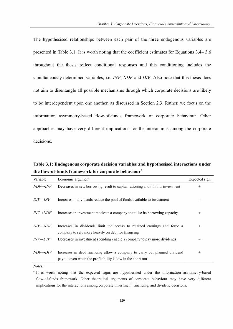
Chapter 3: Corporate Decisions, Financial Constraints and Uncertainty
– 129 –
The hypothesised relationships between each pair of the three endogenous variables are
presented in Table 3.1. It is worth noting that the coefficient estimates for Equations 3.4– 3.6
throughout the thesis reflect conditional responses and this conditioning includes the
simultaneously determined variables, i.e. INV, NDF and DIV. Also note that this thesis does
not aim to disentangle all possible mechanisms through which corporate decisions are likely
to be interdependent upon one another, as discussed in Section 2.3. Rather, we focus on the
information asymmetry-based flow-of-funds framework of corporate behaviour. Other
approaches may have very different implications for the interactions among the corporate
decisions.
Table 3.1: Endogenous corporate decision variables and hypothesised interactions under the flow-of-funds framework for corporate behavioura Variable Economic argument Expected sign
NDF→INV Decreases in new borrowing result to capital rationing and inhibits investment
+
DIV→INV Increases in dividends reduce the pool of funds available to investment
–
INV→NDF Increases in investment motivate a company to utilise its borrowing capacity
+
DIV→NDF Increases in dividends limit the access to retained earnings and force a company to rely more heavily on debt for financing
+
INV→DIV Decreases in investment spending enable a company to pay more dividends
–
NDF→DIV Increases in debt financing allow a company to carry out planned dividend payout even when the profitability is low in the short run
+
Notes: a. It is worth noting that the expected signs are hypothesised under the information asymmetry-based
flow-of-funds framework. Other theoretical arguments of corporate behaviour may have very different
implications for the interactions among corporate investment, financing, and dividend decisions.
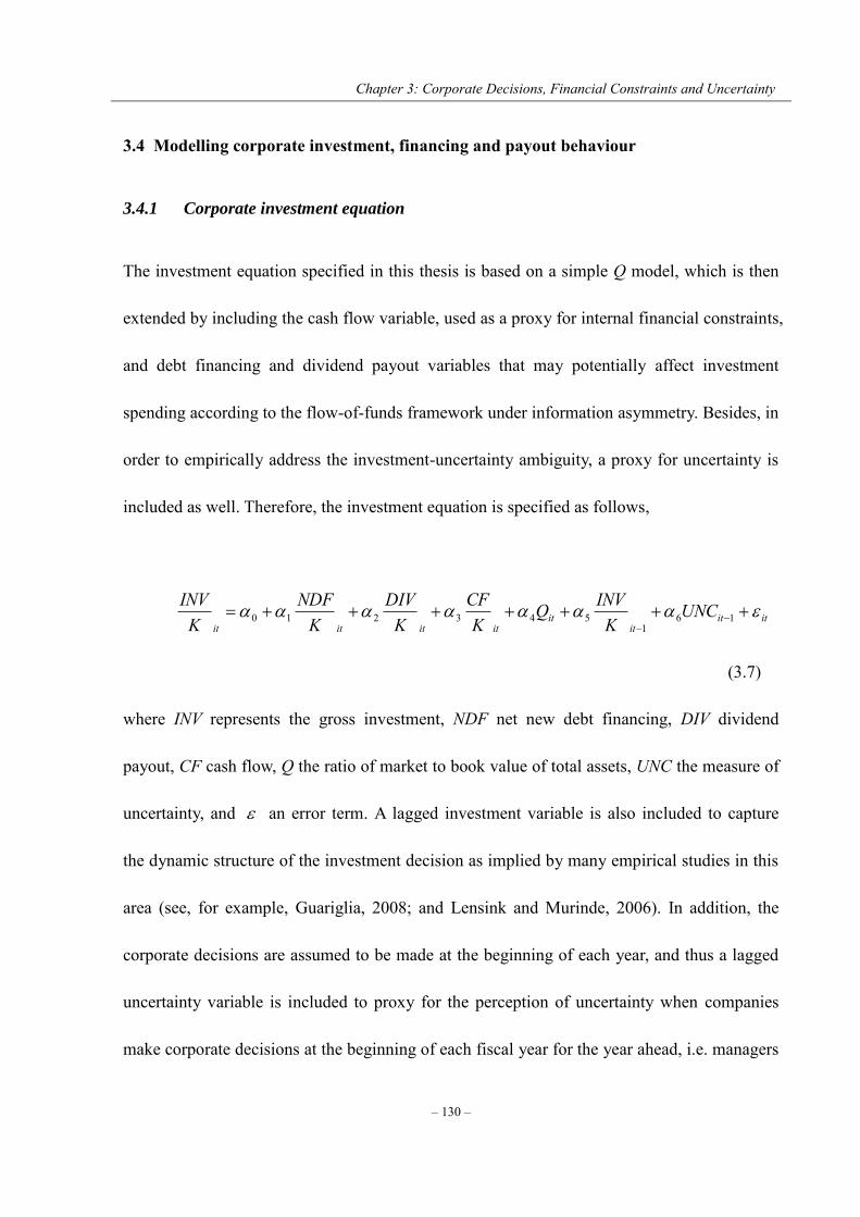
Chapter 3: Corporate Decisions, Financial Constraints and Uncertainty
– 130 –
3.4 Modelling corporate investment, financing and payout behaviour
3.4.1 Corporate investment equation
The investment equation specified in this thesis is based on a simple Q model, which is then
extended by including the cash flow variable, used as a proxy for internal financial constraints,
and debt financing and dividend payout variables that may potentially affect investment
spending according to the flow-of-funds framework under information asymmetry. Besides, in
order to empirically address the investment-uncertainty ambiguity, a proxy for uncertainty is
included as well. Therefore, the investment equation is specified as follows,
ititit
ititititit
UNCK
INVQK
CFK
DIVK
NDFK
INV
16
1543210
(3.7)
where INV represents the gross investment, NDF net new debt financing, DIV dividend
payout, CF cash flow, Q the ratio of market to book value of total assets, UNC the measure of
uncertainty, and an error term. A lagged investment variable is also included to capture
the dynamic structure of the investment decision as implied by many empirical studies in this
area (see, for example, Guariglia, 2008; and Lensink and Murinde, 2006). In addition, the
corporate decisions are assumed to be made at the beginning of each year, and thus a lagged
uncertainty variable is included to proxy for the perception of uncertainty when companies
make corporate decisions at the beginning of each fiscal year for the year ahead, i.e. managers
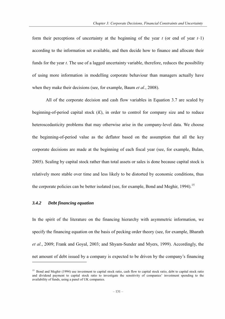
Chapter 3: Corporate Decisions, Financial Constraints and Uncertainty
– 131 –
form their perceptions of uncertainty at the beginning of the year t (or end of year t–1)
according to the information set available, and then decide how to finance and allocate their
funds for the year t. The use of a lagged uncertainty variable, therefore, reduces the possibility
of using more information in modelling corporate behaviour than managers actually have
when they make their decisions (see, for example, Baum et al., 2008).
All of the corporate decision and cash flow variables in Equation 3.7 are scaled by
beginning-of-period capital stock (K), in order to control for company size and to reduce
heteroscedasticity problems that may otherwise arise in the company-level data. We choose
the beginning-of-period value as the deflator based on the assumption that all the key
corporate decisions are made at the beginning of each fiscal year (see, for example, Bulan,
2005). Scaling by capital stock rather than total assets or sales is done because capital stock is
relatively more stable over time and less likely to be distorted by economic conditions, thus
the corporate policies can be better isolated (see, for example, Bond and Meghir, 1994).15
3.4.2 Debt financing equation
In the spirit of the literature on the financing hierarchy with asymmetric information, we
specify the financing equation on the basis of pecking order theory (see, for example, Bharath
et al., 2009; Frank and Goyal, 2003; and Shyam-Sunder and Myers, 1999). Accordingly, the
net amount of debt issued by a company is expected to be driven by the company’s financing
15 Bond and Meghir (1994) use investment to capital stock ratio, cash flow to capital stock ratio, debt to capital stock ratio and dividend payment to capital stock ratio to investigate the sensitivity of companies’ investment spending to the availability of funds, using a panel of UK companies.
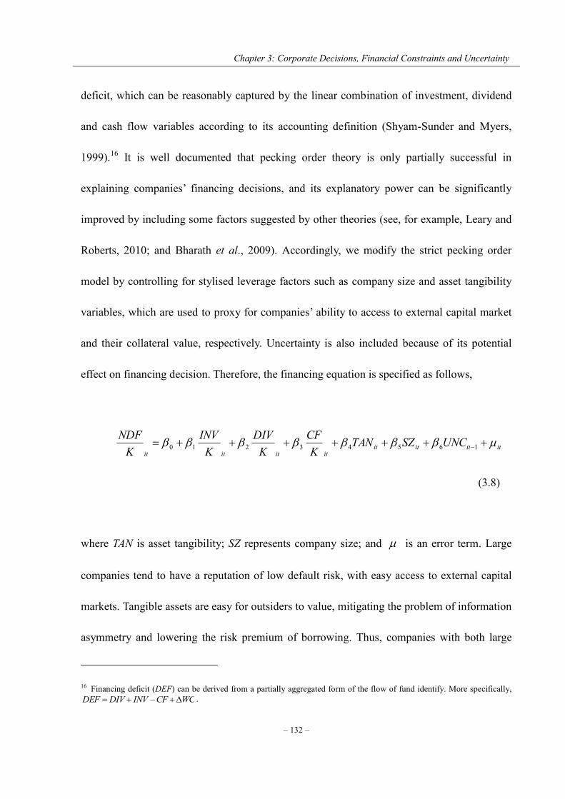
Chapter 3: Corporate Decisions, Financial Constraints and Uncertainty
– 132 –
deficit, which can be reasonably captured by the linear combination of investment, dividend
and cash flow variables according to its accounting definition (Shyam-Sunder and Myers,
1999).16 It is well documented that pecking order theory is only partially successful in
explaining companies’ financing decisions, and its explanatory power can be significantly
improved by including some factors suggested by other theories (see, for example, Leary and
Roberts, 2010; and Bharath et al., 2009). Accordingly, we modify the strict pecking order
model by controlling for stylised leverage factors such as company size and asset tangibility
variables, which are used to proxy for companies’ ability to access to external capital market
and their collateral value, respectively. Uncertainty is also included because of its potential
effect on financing decision. Therefore, the financing equation is specified as follows,
itititititititit
UNCSZTANK
CFK
DIVK
INVK
NDF 16543210
(3.8)
where TAN is asset tangibility; SZ represents company size; and is an error term. Large
companies tend to have a reputation of low default risk, with easy access to external capital
markets. Tangible assets are easy for outsiders to value, mitigating the problem of information
asymmetry and lowering the risk premium of borrowing. Thus, companies with both large
16 Financing deficit (DEF) can be derived from a partially aggregated form of the flow of fund identify. More specifically,WCCFINVDIVDEF .
Chapter 3: Corporate Decisions, Financial Constraints and Uncertainty
– 133 –
size and high level of tangible assets should be able to carry more debt. Besides, greater
uncertainty is likely to exacerbate the degree of information asymmetry between insiders and
outside capital markets, which in turn may generate a more significant cost disadvantage of
external debt financing or even result in credit rationing. Companies, therefore, are likely to
be required to pay a higher premium for new borrowing or be denied loans. Accordingly, we
hypothesise a negative effect of uncertainty on the net amount of debt issued.
3.4.3 Dividend payout equation
The corporate payout equation is modelled on the basis of the signalling hypothesis of
information asymmetry. Since the existing empirical evidence suggests that no single theory
can fully explain the dividend puzzle (see Frankfurter and Wood, 2002), we utilise additional
company characteristics variables, such as ownership structure and financial life cycle stage,
to explain dividend payout behaviour. These factors are generally believed to be the primary
determinants of dividend policy, according to the stylised facts.17 Again, we include the
proxy for uncertainty into the equation as well. The dividend model is specified as follows,
ititit
ititititit
UNCTEREOWN
KCF
KNDF
KINV
KDIV
16543210
(3.9)
17 Some studies also employ lagged dividend status as an explanatory variable (see, for example, Ferris et al., 2009; and Khan, 2006). However, Fama and French (2001) argue that including a lagged dividend status is problematic because the resultant model seeks to explain a company’s current dividend decision on the basis of the same decision made recently by the same company. Therefore, we ignore lagged dividend status in modelling corporate payout behaviour.
Chapter 3: Corporate Decisions, Financial Constraints and Uncertainty
– 134 –
where OWN is insider ownership structure; RE/TE is a retained earnings-to-total equity ratio,
a proxy for a company’s financial life cycle stage; and is an error terms. Cash flow and
retained earnings-to-total equity ratio are expected to have positive effects on dividend payout,
whilst insider ownership is expected to have a negative effect. The relationship between
uncertainty and dividend payout, however, is not so clear-cut. It is reasonable to argue that,
with asymmetric information, managers adjust dividend payouts upward or downward only
on a permanent change in their business environment. If the prospects are uncertain, managers
may choose to wait for more information rather than adjust dividend policy immediately, for
fear of sending wrong information to the markets. If this argument is supported by empirical
evidence, uncertainty may dampen the response of dividend payout to cash flow. It is equally
plausible to argue that a company’s prospects are less predictable under uncertainty, so that
managers’ confidence in maintaining dividend payouts at certainty level will collapse. Thus,
managers’ perception of uncertainty may result in a cut in dividend payouts.18 We therefore
expect the effect of uncertainty on corporate dividend payout to be neutral or negative.
3.5 Data and preliminary analysis
3.5.1 Data and measurement
The data are collected from the Worldscope database via Thomson One Banker Analytics. The
18 Sant and Cowan (1994) assert that, if managers’ confidence interval on the company’s future performances no longer reassures them that they will be able to continue the current payout, they may cut or even omit dividends. Both decreased expected performance and increased variance of future performances may make managers’ confidence interval less reassuring
Chapter 3: Corporate Decisions, Financial Constraints and Uncertainty
– 135 –
initial sample includes all companies listed on the London Stock Exchange (LSE), including
both active and inactive companies within the period 1999–2008. We then discard utilities
(Standard Industrial Classification (SIC) code 4900–4949), and financial companies (SIC
code 6000–6999). Companies that do not have complete records for the key data, such as
capital investment committed, new debt issued and cash dividends paid, and those with less
than five years of continuous observations are dropped from our sample. We also exclude
company-year observations with negative cash flow from our sample. An unbalanced panel of
company-level data is formed to avoid survivorship bias.19 Stock prices are retrieved from
DataStream for the same batch of companies over the same period of time.
To make full use of the data, a company-year observation is included in the sample for
single equation analyses as long as it has records on the relevant variables in determining the
corporate decision under investigation. For example, our single equation analysis for
corporate investment behaviour utilises all the company-year observations which have records
for INV/K, NDF/K, DIV/K, CF/K, Q, (INV/K)-1 and UNC. However, for the simultaneous
equations analyses, a company-year observation can be utilised only if it has complete records
on all the relevant variables in determining the three corporate decisions. The number of
company-year observations included in the final sample for our simultaneous equations
analyses therefore reduces to 2,791.
19 The empirical investigation is based on an unbalanced panel of company-level data, which means that not only active but also dead and suspended listed companies on LSE are included in the sample.

Chapter 3: Corporate Decisions, Financial Constraints and Uncertainty
– 136 –
Table 3.2: Description of main variables used in Chapter 3a
Gross investment (INV):
The sum of the changes in book value of net property, plant and equipment and depreciation expensesb
Net debt financing (NDF):
The change in the book value of long-term debt
Dividends (DIV):
The reported total dividends paid on common stock, including extra and special dividends
Cash flow (CF):
The sum of net income and depreciation expenses
Capital stock (K):
The book value of tangible fixed assets
Average Q (Q):
The ratio of the market value of equity plus the book value of debt to the book value of total assets
Company size (SZ):
The natural logarithm of the book value of total assets
Asset tangibility (TAN):
The ratio of the book value of net property, plant and equipment to the book value of total assets
Ownership structure (OWN):
The percentage of common share outstanding that is held by insiders
Retained earnings-to-total equity ratio (RE/TE):
The ratio of the book value of retained earnings in balance sheet to the book value of total common equity
Uncertainty measure 1 (UNC1):
The difference between the highest and the lowest prices normalised by the mean over the period
Uncertainty measure 2 (UNC2):
The conventional standard deviation of daily stock market returns over the period
Uncertainty measure 3 (UNC3):
The average of conditional standard deviations of daily stock returns over the period
Financial leverage index (FLI):
The ratio of return on average assets to return on average equity
Notes: a. The definition and measurement of the variables are based on the existing literature. b. The data are collected from the Worldscope database via Thomson One Banker Analytics, except the daily
share prices used to construct uncertainty measures 2 and 3, which were obtained from the DataStream
database.
Chapter 3: Corporate Decisions, Financial Constraints and Uncertainty
– 137 –
The definition of each variable used in this chapter is described in Table 3.2. As
discussed in Section 3.2, constructing an appropriate proxy for uncertainty is the primary
challenge faced by studies investigating the effects of uncertainty on corporate behaviour. We
construct three proxies for uncertainty based on stock prices, under the assumption that all the
information about a company’s fundamentals and prospects will be properly transmitted into
its share price.20 The first proxy for uncertainty is share price volatility (UNC1), which is
measured as the difference between the highest and the lowest prices normalised by the mean
value for each year. The second proxy is the conventional standard deviation of daily stock
market returns for each year (UNC2). Besides, the possible volatility clustering effect of stock
market returns motivates us to derive a third measure of uncertainty (UNC3), which is
estimated from a GARCH (1, 1) model specified as follows,
tttt uRRR 22110 (3.10)
212
2110
2 ttt u (3.11)
where Rt denotes the stock market return at time t, and 2t denotes the conditional variance of
the daily stock market return at time t. Both the conditional mean and conditional variance
equations are estimated company by company over the entire sample period under
20 The proxies for uncertainty based on stock market information are expected to be forward-looking indicators and able to capture the overall uncertainty associated with the changing aspects of a company’s business environment. Share prices tend to fluctuate more when the prospects are less predictable.
Chapter 3: Corporate Decisions, Financial Constraints and Uncertainty
– 138 –
investigation. To construct a proxy for uncertainty on yearly basis, we first take the square
root of the estimated daily conditional variances to obtain the daily conditional standard
deviation, and then calculate the average of the daily conditional standard deviations of the
stock market returns over each year as an uncertainty measure for the corresponding period.
All the three proxies for uncertainty are derived from information on the volatility of
individual companies’ stock prices, and therefore are forward looking in nature. However, the
main concern is that the high-frequency stock market data may reflect not only companies’
fundamentals but also bubbles and fads, making this type of proxy for uncertainty too noisy
(see, for example, Bond and Cummins, 2004; and Bloom et al., 2007). In particular, the use of
daily stock returns may produce extremely noisy proxies for uncertainty. Thus, among the
three alternatives, UNC1 is treated as the primary measure of uncertainty, because it is
constructed as the normalised difference between yearly high and yearly low prices, and
hence should be better able to match companies’ annual financial data and to reduce the
impact of high-frequency noise that may be present in the daily observations. UNC2 and
UNC3 are used as supplementary measures of uncertainty. 21 Therefore, our empirical
findings on the effects of uncertainty on corporate decisions are mainly drawn from the sign
and significance level of the coefficient on UNC1 in the corresponding equations.
21 Lensink and Murinde (2006) also point out that the standard deviation of daily stock market returns and the average of daily conditional standard deviations of stock market returns do not measure annual volatility but the average daily volatility in the respective year. Another reason for using UNC1 as our primary measure of uncertainty is that the data on this variable, as well as the other accounting items, are collected from the Worldscope database, whereas the daily share prices used to compute UNC2 and UNC3 are collected from the DataStream database. Once the two datasets are merged, the number of observations declines significantly.
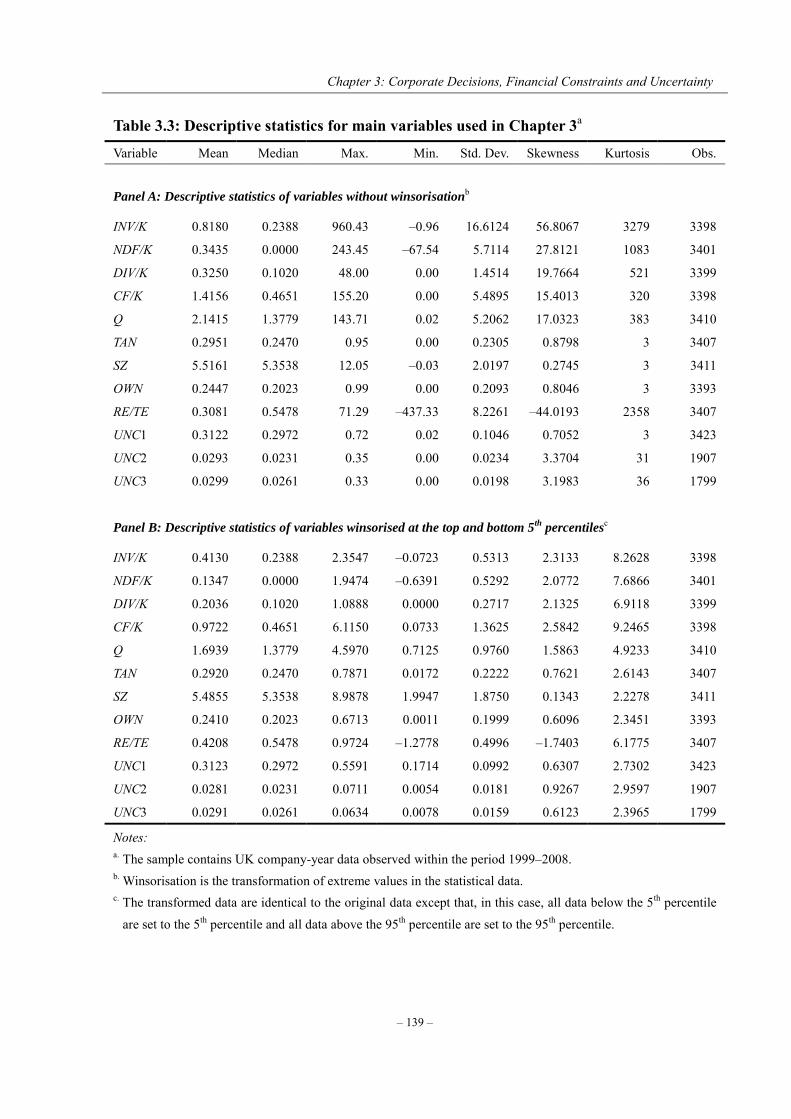
Chapter 3: Corporate Decisions, Financial Constraints and Uncertainty
– 139 –
Table 3.3: Descriptive statistics for main variables used in Chapter 3a
Variable Mean Median Max. Min. Std. Dev. Skewness Kurtosis Obs.
Panel A: Descriptive statistics of variables without winsorisationb
INV/K 0.8180 0.2388 960.43 –0.96 16.6124 56.8067 3279 3398
NDF/K 0.3435 0.0000 243.45 –67.54 5.7114 27.8121 1083 3401
DIV/K 0.3250 0.1020 48.00 0.00 1.4514 19.7664 521 3399
CF/K 1.4156 0.4651 155.20 0.00 5.4895 15.4013 320 3398
Q 2.1415 1.3779 143.71 0.02 5.2062 17.0323 383 3410
TAN 0.2951 0.2470 0.95 0.00 0.2305 0.8798 3 3407
SZ 5.5161 5.3538 12.05 –0.03 2.0197 0.2745 3 3411
OWN 0.2447 0.2023 0.99 0.00 0.2093 0.8046 3 3393
RE/TE 0.3081 0.5478 71.29 –437.33 8.2261 –44.0193 2358 3407
UNC1 0.3122 0.2972 0.72 0.02 0.1046 0.7052 3 3423
UNC2 0.0293 0.0231 0.35 0.00 0.0234 3.3704 31 1907
UNC3 0.0299 0.0261 0.33 0.00 0.0198 3.1983 36 1799
Panel B: Descriptive statistics of variables winsorised at the top and bottom 5th
percentilesc
INV/K 0.4130 0.2388 2.3547 –0.0723 0.5313 2.3133 8.2628 3398
NDF/K 0.1347 0.0000 1.9474 –0.6391 0.5292 2.0772 7.6866 3401
DIV/K 0.2036 0.1020 1.0888 0.0000 0.2717 2.1325 6.9118 3399
CF/K 0.9722 0.4651 6.1150 0.0733 1.3625 2.5842 9.2465 3398
Q 1.6939 1.3779 4.5970 0.7125 0.9760 1.5863 4.9233 3410
TAN 0.2920 0.2470 0.7871 0.0172 0.2222 0.7621 2.6143 3407
SZ 5.4855 5.3538 8.9878 1.9947 1.8750 0.1343 2.2278 3411
OWN 0.2410 0.2023 0.6713 0.0011 0.1999 0.6096 2.3451 3393
RE/TE 0.4208 0.5478 0.9724 –1.2778 0.4996 –1.7403 6.1775 3407
UNC1 0.3123 0.2972 0.5591 0.1714 0.0992 0.6307 2.7302 3423
UNC2 0.0281 0.0231 0.0711 0.0054 0.0181 0.9267 2.9597 1907
UNC3 0.0291 0.0261 0.0634 0.0078 0.0159 0.6123 2.3965 1799
Notes: a. The sample contains UK company-year data observed within the period 1999–2008. b. Winsorisation is the transformation of extreme values in the statistical data. c. The transformed data are identical to the original data except that, in this case, all data below the 5th percentile
are set to the 5th percentile and all data above the 95th percentile are set to the 95th percentile.

Chapter 3: Corporate Decisions, Financial Constraints and Uncertainty
– 140 –
Panel A of Table 3.3 presents the descriptive statistics for the main variables from our
raw data. As is evident, extreme values appear in almost all the variables, especially those that
are constructed as ratios. Baum et al. (2008) point out that the values of the
investment-to-capital, cash flow-to-capital, debt-to-capital ratios and Tobin’s Q outside the 5th
and 95th percentile range should be judged implausible, and thus should be screened to reduce
the potential impact of outliers upon the parameter estimates. Accordingly, we winsorise all
the variables used in our analysis at the top and bottom 5th percentiles of their respective
distributions. Specifically, the winsorisation transformation would set all observations below
the 5th percentile equal to the 5th percentile, and observations above the 95th percentile equal
to the 95th percentile. Such a transformation not only reduces the potential impact of outliers
but also allows the full use of observations. Panel B reports the descriptive statistics after such
a transformation is undertaken. It shows that the maximum values of INV/K, NDF/K and
DIV/K reduce from 960.43, 243.45 and 48.00 to 2.35, 1.95 and 1.09, respectively. The
standard deviations for each of these variables reduce from 16.61, 5.71 and 1.45 to 0.53, 0.53
and 0.27, respectively, and more importantly, their distributions are more close to normality
after the transformation, as suggested by the skewness and kurtosis statistics. Since the
winsorisation estimators are expected to be more robust, our empirical results presented
hereafter are, therefore, obtained by using the winsorised variables.22
22 It is believed that winsorisation is superior to the more standard transformations such as trimming. Winsorisation not only reduces the influences of outliers, but also allows us to make full use of the sample observations (see, for example, Chay and Suh, 2009).
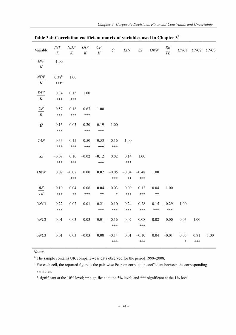
Chapter 3: Corporate Decisions, Financial Constraints and Uncertainty
– 141 –
Table 3.4: Correlation coefficient matrix of variables used in Chapter 3a
Variable K
INV K
NDF K
DIV K
CF
Q TAN SZ OWN TERE UNC1 UNC2 UNC3
KINV
1.00
KNDF
0.38b ***c
1.00
KDIV
0.34 ***
0.15 ***
1.00
KCF
0.57 ***
0.18 ***
0.67 ***
1.00
Q 0.13 ***
0.03
0.20 ***
0.19 ***
1.00
TAN –0.33 ***
–0.15 ***
–0.50 ***
–0.53 ***
–0.16 ***
1.00
SZ –0.08 ***
0.10 ***
–0.02
–0.12 ***
0.02
0.14 ***
1.00
OWN 0.02
–0.07 ***
0.00
0.02
–0.05 ***
–0.04 **
–0.48 ***
1.00
TERE
–0.10
*** –0.04
** 0.06 ***
–0.04 **
–0.03 *
0.09 ***
0.12 ***
–0.04 **
1.00
UNC1 0.22 ***
–0.02
–0.01
0.21 ***
0.10 ***
–0.24 ***
–0.28 ***
0.15 ***
–0.29 ***
1.00
UNC2 0.01
0.03
–0.03
–0.01
–0.16 ***
0.02
–0.08 ***
0.02
0.00
0.03
1.00
UNC3 0.01
0.03
–0.03
0.00
–0.14 ***
0.01
–0.10 ***
0.04
–0.01
0.05 *
0.91 ***
1.00
Notes: a. The sample contains UK company-year data observed for the period 1999–2008. b. For each cell, the reported figure is the pair-wise Pearson correlation coefficient between the corresponding
variables. c. * significant at the 10% level; ** significant at the 5% level; and *** significant at the 1% level.
Chapter 3: Corporate Decisions, Financial Constraints and Uncertainty
– 142 –
The pair-wise correlation among the main variables is presented in Table 3.4. It shows
that the three endogenous variables (namely, INV/K, NDF/K and DIV/K) are significantly
correlated with one another, and that the predetermined cash flow variable (CF/K) is
significantly correlated with all three endogenous variables. However, the correlation
coefficients between endogenous variables are uniformly positive, which is not entirely
consistent with the implications of flow-of-funds framework. It is also evident that the
uncertainty proxy (UNC1) is significantly and positively correlated with corporate investment
(INV/K), and weakly and negatively correlated with the new debt financing ratio (NDF/K) and
dividend payout ratio (DIV/K). Finally, the correlations between the endogenous variables and
other relevant exogenous variables are also informative. According to Table 3.4, INV/K is
significantly and positively correlated with investment opportunities (Q); NDF/K is positively
correlated with company size (SZ) but negatively correlated with asset tangibility (TAN);
DIV/K is positively correlated with company’s financial life cycle stage (RE/TE) but its
correlation with insider ownership (OWN) is rather weak. In addition, there is no evidence of
near multicollinearity presented in the correlation coefficient matrix.
3.5.2 Preliminary diagnostic tests
Since the simultaneous determination of corporate investment, financing and payout decisions
hypothesised in this thesis is based on the reduced form flow-of-funds identity alongside a
number of associated assumptions, it is desirable to explicitly test the validity of these
assumptions using our dataset before we proceed to the analysis of simultaneity among the set
Chapter 3: Corporate Decisions, Financial Constraints and Uncertainty
– 143 –
of corporate decisions.
3.5.2.1 Test for validity of the reduced form flow-of-funds identity
To derive the reduced form flow-of-funds identify, we assume that external equity financing is
considered by managers as the last resort and thus rarely used in practice. Base on the
assumption that external equity finance is a less significant source of funds for listed
companies after their IPOs (see Shyam-Sunder and Myers, 1999; and Cleary et al., 2007), we
drop it from the flow-of-funds framework. To verify the assumption, we empirically test
whether the reduced form flow-of-funds identity holds with respect to the UK-listed
companies. Given the difficulties in measuring external equity financing in practice, we verify
the validity of the reduced form identity and the associated assumption by testing the equality
of the uses and sources of funds as specified in Equation 3.3. If the reduced form
flow-of-funds identity is supported by our dataset, then external equity finance can be
considered as a rarely used source of funds, and therefore can be dropped from the
flow-of-funds framework.
The main uses and sources of funds, apart from external equity finance, for the
UK-listed companies over the period under investigation are summarised in Table 3.5. The
total uses and sources of funds are compared under a t-test framework. Both paired and
unpaired mean-comparison tests are carried out to test for equality between the uses and
sources of funds. According to the evidence obtained from the panel of UK-listed companies,
the reduced form flow-of-funds identity is empirically supported in most of instances,
Chapter 3: Corporate Decisions, Financial Constraints and Uncertainty
– 144 –
suggesting that the sum of investment outlays, dividend payouts and change in working
capital is approximately equal to the sum of external debt financing and internally generated
cash flow. The uses and sources of funds identity is only rejected for years 2000 and 2007
under the paired t-test and for year 2007 under the unpaired t-test. The rejections of equality
for in both cases are likely to be caused by the extreme economic environment under the
dot-com crisis in 2000 and the global financial crisis starts in 2007, respectively. Overall, the
reduced form flow-of-funds identity is verified by the pooled UK company-year observations
over the entire period under investigation. We, therefore, can conclude that the reduced form
flow-of-funds identity holds in the context of our investigation.
Another interesting result observed from Table 3.5 is that, compared with capital
investment and dividends spending, the funds spent on working capital (ΔWC) is of minor
significance for most of the years. The mean values for capital investment, dividend payout
and spending on working capital made by UK-listed companies during the period from 1999
to 2008 are 74.28, 31.09 and 0.80 million pounds, respectively. The empirical evidence
clearly shows that compared with capital investment and dividend outlays the funds spent on
working capital (∆WC) is of minor significance for UK-listed companies. In addition, the
signs on the net spending on working capital are not consistent over the period under
investigation, with 5 positive and 5 negative values observed during the ten-year observation
window. This evidence empirically rationalises the view that net changes in working capital
can be considered as residual to balancing the uses and sources of funds.
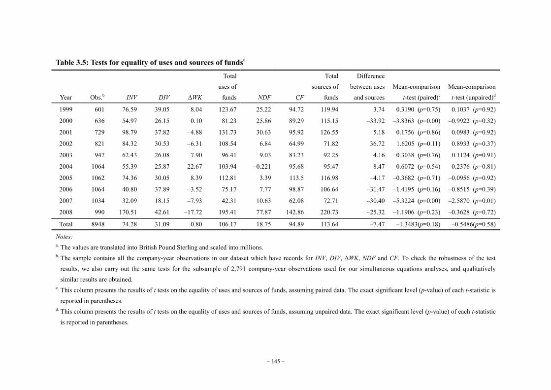
– 145 –
Table 3.5: Tests for equality of uses and sources of fundsa
Year Obs.b INV DIV ΔWK
Total uses of
funds NDF CF
Total sources of
funds
Difference between uses
and sources Mean-comparison
t-test (paired)c Mean-comparison
t-test (unpaired)d
1999 601 76.59 39.05 8.04 123.67 25.22 94.72 119.94 3.74 0.3190 (p=0.75) 0.1037 (p=0.92)
2000 636 54.97 26.15 0.10 81.23 25.86 89.29 115.15 –33.92 –3.8363 (p=0.00) –0.9922 (p=0.32)
2001 729 98.79 37.82 –4.88 131.73 30.63 95.92 126.55 5.18 0.1756 (p=0.86) 0.0983 (p=0.92)
2002 821 84.32 30.53 –6.31 108.54 6.84 64.99 71.82 36.72 1.6205 (p=0.11) 0.8933 (p=0.37)
2003 947 62.43 26.08 7.90 96.41 9.03 83.23 92.25 4.16 0.3038 (p=0.76) 0.1124 (p=0.91)
2004 1064 55.39 25.87 22.67 103.94 –0.221 95.68 95.47 8.47 0.6072 (p=0.54) 0.2376 (p=0.81)
2005 1062 74.36 30.05 8.39 112.81 3.39 113.5 116.98 –4.17 –0.3682 (p=0.71) –0.0956 (p=0.92)
2006 1064 40.80 37.89 –3.52 75.17 7.77 98.87 106.64 –31.47 –1.4195 (p=0.16) –0.8515 (p=0.39)
2007 1034 32.09 18.15 –7.93 42.31 10.63 62.08 72.71 –30.40 –5.3224 (p=0.00) –2.5870 (p=0.01)
2008 990 170.51 42.61 –17.72 195.41 77.87 142.86 220.73 –25.32 –1.1906 (p=0.23) –0.3628 (p=0.72)
Total 8948 74.28 31.09 0.80 106.17 18.75 94.89 113.64 –7.47 –1.3483(p=0.18) –0.5486(p=0.58)
Notes: a. The values are translated into British Pound Sterling and scaled into millions. b. The sample contains all the company-year observations in our dataset which have records for INV, DIV, ΔWK, NDF and CF. To check the robustness of the test
results, we also carry out the same tests for the subsample of 2,791 company-year observations used for our simultaneous equations analyses, and qualitatively similar results are obtained.
c. This column presents the results of t tests on the equality of uses and sources of funds, assuming paired data. The exact significant level (p-value) of each t-statistic is reported in parentheses.
d. This column presents the results of t tests on the equality of uses and sources of funds, assuming unpaired data. The exact significant level (p-value) of each t-statistic is reported in parentheses.

Chapter 3: Corporate Decisions, Financial Constraints and Uncertainty
– 146 –
Overall, the empirical evidence presented in Table 3.5 clearly demonstrates that the
UK-listed companies raise funds mainly from internally generated cash flow and external debt
finance, and spend it chiefly on capital investment and dividend payouts. Therefore, it is valid
to derive the simultaneous equations system based on the reduced form flow-of-funds identity,
which allows us to focus directly on the possible interactions among corporate investment,
financing and payout decisions made by UK-listed companies.
3.5.2.2 Test for endogeneity of corporate decisions variables
Although the potential simultaneity that may exist among corporate investment, financing and
payout decisions has been rationalised from a theoretical perspective, it is still important to
test the hypothesis explicitly before proceeding to the simultaneous equations analysis of the
set of corporate decisions. If the variables specified as endogenous can in fact be treated as
exogenous, the coefficients estimated using simultaneous analyses are likely to be inefficient.
To empirically justify the simultaneity of corporate decisions, we apply both the Hausman test
for endogeneity and an enhanced test for endogeneity developed by Baum et al. (2007) to the
corporate decision variables that are specified as endogenous in the simultaneous equations
system. The enhanced test for endogeneity is equivalent to the Hausman test under
conditional homoscedasticity. Unlike the Hausman test, the enhanced test for endogeneity
provided by Baum et al. (2007) is robust to various violations of conditional homoscedasticity.
Under the null hypothesis of the endogeneity test, the might-be-endogenous variables can
actually be treated as exogenous, and the test statistic follows a Chi-squared distribution with
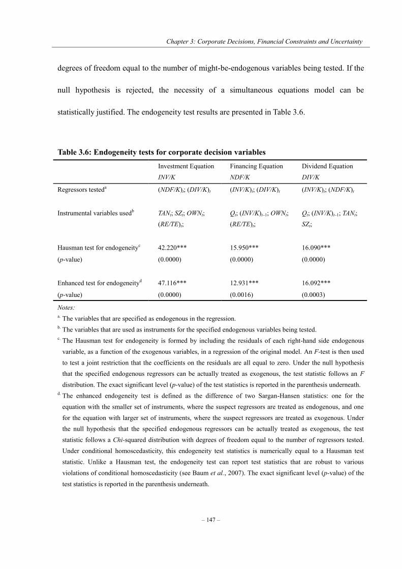
Chapter 3: Corporate Decisions, Financial Constraints and Uncertainty
– 147 –
degrees of freedom equal to the number of might-be-endogenous variables being tested. If the
null hypothesis is rejected, the necessity of a simultaneous equations model can be
statistically justified. The endogeneity test results are presented in Table 3.6.
Table 3.6: Endogeneity tests for corporate decision variables
Investment Equation INV/K
Financing Equation NDF/K
Dividend Equation DIV/K
Regressors testeda (NDF/K)t; (DIV/K)t (INV/K)t; (DIV/K)t (INV/K)t; (NDF/K)t
Instrumental variables usedb TANt; SZt; OWNt; (RE/TE)t;
Qt; (INV/K)t–1; OWNt; (RE/TE)t;
Qt; (INV/K)t–1; TANt; SZt;
Hausman test for endogeneityc 42.220*** 15.950*** 16.090***
(p-value) (0.0000) (0.0000) (0.0000)
Enhanced test for endogeneityd 47.116*** 12.931*** 16.092***
(p-value) (0.0000) (0.0016) (0.0003)
Notes: a. The variables that are specified as endogenous in the regression. b. The variables that are used as instruments for the specified endogenous variables being tested. c. The Hausman test for endogeneity is formed by including the residuals of each right-hand side endogenous
variable, as a function of the exogenous variables, in a regression of the original model. An F-test is then used to test a joint restriction that the coefficients on the residuals are all equal to zero. Under the null hypothesis that the specified endogenous regressors can be actually treated as exogenous, the test statistic follows an F distribution. The exact significant level (p-value) of the test statistics is reported in the parenthesis underneath.
d. The enhanced endogeneity test is defined as the difference of two Sargan-Hansen statistics: one for the equation with the smaller set of instruments, where the suspect regressors are treated as endogenous, and one for the equation with larger set of instruments, where the suspect regressors are treated as exogenous. Under the null hypothesis that the specified endogenous regressors can be actually treated as exogenous, the test statistic follows a Chi-squared distribution with degrees of freedom equal to the number of regressors tested. Under conditional homoscedasticity, this endogeneity test statistics is numerically equal to a Hausman test statistic. Unlike a Hausman test, the endogeneity test can report test statistics that are robust to various violations of conditional homoscedasticity (see Baum et al., 2007). The exact significant level (p-value) of the
test statistics is reported in the parenthesis underneath.
Chapter 3: Corporate Decisions, Financial Constraints and Uncertainty
– 148 –
According to Table 3.6, the results of both tests suggest that the exogeneity of debt
financing and dividend payout variables in the investment equation can be firmly rejected;
again, that of investment and dividend payout variables in the debt financing equation can be
firmly rejected; finally, that of investment and debt financing variables in the payout equation
can be firmly rejected as well. An important implication is that it is inappropriate and invalid
to treat these endogenous variables as exogenous, and thus a simultaneous equations model is
necessary in practice. The existing literature in corporate finance that ignores the endogeneity
of investment, financing and payout decisions is likely to generate misleading results and lead
to inappropriate inferences, which may bias our understanding of corporate behaviour.
Therefore, corporate investment, financing and payout decisions should be better considered
as a joint decision-making procedure. A preferred strategy is to simultaneously estimate the
corporate decision equations within a system which allows for the interactions among the set
of corporate decisions.
3.5.2.3 Test for exogeneity of cash flow variable
To derive the simultaneous equations system, we also assume that internally generated cash
flow is predetermined by past corporate real and financial decisions (Dhrymes and Kurz, 1967;
and McCabe, 1979), and thus can be treated as exogenous to the system. It is, therefore, also
desirable to test the validity of this assumption explicitly. For this reason, we also carry out
endogeneity tests for the cash flow variable in investment, financing and payout equations,
respectively. The test results are reported in Table 3.7.
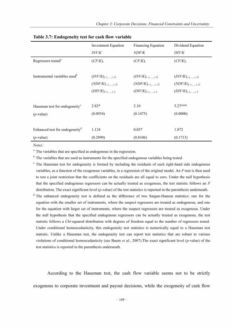
Chapter 3: Corporate Decisions, Financial Constraints and Uncertainty
– 149 –
Table 3.7: Endogeneity test for cash flow variable
Investment Equation
INV/K
Financing Equation
NDF/K
Dividend Equation
DIV/K
Regressors testeda (CF/K)t (CF/K)t (CF/K)t
Instrumental variables usedb (INV/K)t–1,…, t–3;
(NDF/K)t–1,…, t–3;
(DIV/K)t–1,…, t–3
(INV/K)t–1,…, t–3;
(NDF/K)t–1,…, t–3;
(DIV/K)t–1,…, t–3
(INV/K)t–1,…, t–3;
(NDF/K)t–1,…, t–3;
(DIV/K)t–1,…, t–3
Hausman test for endogeneityc 2.82* 2.10 5.27***
(p-value) (0.0934) (0.1475) (0.0000)
Enhanced test for endogeneityd 1.124 0.057 1.872
(p-value) (0.2890) (0.8106) (0.1713)
Notes: a. The variables that are specified as endogenous in the regression. b. The variables that are used as instruments for the specified endogenous variables being tested. c. The Hausman test for endogeneity is formed by including the residuals of each right-hand side endogenous
variables, as a function of the exogenous variables, in a regression of the original model. An F-test is then used to test a joint restriction that the coefficients on the residuals are all equal to zero. Under the null hypothesis that the specified endogenous regressors can be actually treated as exogenous, the test statistic follows an F distribution. The exact significant level (p-value) of the test statistics is reported in the parenthesis underneath.
d. The enhanced endogeneity test is defined as the difference of two Sargan-Hansen statistics: one for the equation with the smaller set of instruments, where the suspect regressors are treated as endogenous, and one for the equation with larger set of instruments, where the suspect regressors are treated as exogenous. Under the null hypothesis that the specified endogenous regressors can be actually treated as exogenous, the test statistic follows a Chi-squared distribution with degrees of freedom equal to the number of regressors tested. Under conditional homoscedasticity, this endogeneity test statistics is numerically equal to a Hausman test statistic. Unlike a Hausman test, the endogeneity test can report test statistics that are robust to various violations of conditional homoscedasticity (see Baum et al., 2007).The exact significant level (p-value) of the
test statistics is reported in the parenthesis underneath.
According to the Hausman test, the cash flow variable seems not to be strictly
exogenous to corporate investment and payout decisions, while the exogeneity of cash flow
Chapter 3: Corporate Decisions, Financial Constraints and Uncertainty
– 150 –
variable with respect to the debt financing decision cannot be rejected. The Hausman test
results suggest that current cash flow is not purely determined by previous corporate decisions,
but also to some extent depend on concurrent decisions. However, the assumption of the
exogeneity of the cash flow variable is empirically verified by the enhanced test for
endogeneity developed by Baum et al. (2007). The null hypothesis that the cash flow variable
can be treated as exogenous cannot be rejected throughout the tests regarding all the three
equations. Accordingly, there should be no significant endogenous effect of cash flow variable
on the estimates. The cash flow variable, therefore, can be validly taken as an exogenous
variable in the simultaneous equations system, allowing us to focus directly on the
simultaneity among corporate investment, financing and payout decisions. All in all, the
preliminary tests presented in this section are reasonably satisfactory for us to move on to the
joint determinations of corporate decisions as implied by the flow-of-funds framework for
corporate behaviour.
3.6 Empirical results and implications for corporate behaviour
3.6.1 Single equation analyses
Although the purpose of the study is to investigate the simultaneity among corporate
investment, financing and payout decisions, it is desirable to first apply the single equation
estimation technique to the corporate behaviour equations separately. The single equation
estimation results presented in this section are comparable to those provided by the previous

Chapter 3: Corporate Decisions, Financial Constraints and Uncertainty
– 151 –
studies which ignore the interdependence of the decision-making processes that we aim to
investigate.
Given the endogeneity of the corporate decision variables and the dynamic structures
of the corporate behaviour models, we estimate Equations 3.7, 3.8 and 3.9 separately using
the system generalised methods of moments (system-GMM) estimators. This approach is an
efficient extension of the first-difference generalised methods of moments (difference-GMM)
estimators developed by Arellano and Bond (1991).23 It combines an equation in differences
of the variables with an equation in levels of variables to form a system, in which lagged
levels are used as instruments for the differenced equation and lagged differences are used as
instruments for the level equation (Aerllano and Bover, 1995; and Blundell and Bond,
1998).24 The use of instruments in such a way is considered as a possible solution to the
endogeneity problems as well as the weak instrument problems.
In the implementation of system-GMM estimators, we are also confronted with the
choice of using one-step or two-step estimation. The one-step estimators assume
homoscedastic errors, whereas the two-step estimators generate heteroscedasticity-consistent
standard errors. Thus, the two-step estimators are expected to be asymptotically more efficient
23 Arellano and Bond’s (1991) difference-GMM estimator can be subject to a large downward bias and very low precisions as a result of weak instruments in situations where the series are highly persistent and/or the relative variance of the fixed effects increases even for large n when t is small. 24 The system-GMM estimator uses equations in first-differences, from which the company-specific effects are eliminated by the transformation, and for which endogenous variables lagged two or more periods will be valid instruments provided there is no serial correlation in the time-varying component of the error terms. These differenced equations are then combined with equations in levels for which the instruments used must be orthogonal to the company-specific effects. Blundell and Bond (1998) show that in autoregressive distributed lag models, the first-differences of the series can be uncorrelated with the company-specific effect provided that the series have stationary means.

Chapter 3: Corporate Decisions, Financial Constraints and Uncertainty
– 152 –
than their one-step counterparts. However the reported standard errors in two-step estimation
tend to be downward biased, it is important to use the finite-sample correction to the standard
errors computed in two-step estimation (Roodman, 2009). We therefore resort to the two-step
system-GMM estimators with finite-sample correction to estimate the structural equations for
corporate behaviour. The two-step system-GMM estimation results are obtained using Stata
11 as implemented by Roodman (2009).
Given the fact that the reliability of the system-GMM method depends crucially on the
validity of instruments and serial correlation of the error terms, we check them with Hensen’s
J tests of over-identifying restrictions and Arellano-Bond’s tests of serial correlation,
respectively. Year dummies also are included in all of the equations to account for the time
effect that cannot be captured by the included regressors.25 Tables 3.8–3.10 present the
estimation and testing results corresponding to the corporate investment, borrowing and
dividend equations, respectively.
3.6.1.1 Investment equation estimation results
Columns 2, 3 and 4 of Table 3.8 report the estimations and test results for three variants of the
investment model specified as Equation 3.7. The three alternative proxies for uncertainty
described in the previous section, namely, UNC1, UNC2 and UNC3, are used in the three
25 To implement GMM estimations, it is assumed that errors are only correlated within individuals, not across them. Therefore, it is almost always desirable to include time dummies in order to remove universal time-related shocks from the errors (Roodman, 2009).
Chapter 3: Corporate Decisions, Financial Constraints and Uncertainty
– 153 –
model variants, respectively. Given the drawback of constructing uncertainty measures using
high-frequency stock return information, we treat the results obtained from model variant 1, in
which UNC1 is used as the proxy for uncertainty, as our primary results.
Concentrating on the primary results presented in column 2, three features of these
results are of particular interest. First, both the borrowing (NDF/K) and dividend (DIV/K)
variables appear to be significant in the investment equation at the 1% and 5% significance
level respectively. This result suggests that a company’s financial decisions do have impacts
on its real decisions in reality, so that Modigliani-Miller’s independence proposition should be
firmly rejected based on the evidence from UK-listed companies.
Second, the significantly positive relationship between investment and dividend found
in the pair-wise correlation analysis (see Table 3.4) is reversed to be significantly negative
when the full structural investment equation is estimated. The statistically significant and
negative effect of dividend payouts on investment outlays lends strong empirical support to
the flow-of-funds framework, in which investment outlays and dividend payouts are viewed
as competing uses of limited funds and thus should not vary in the same direction. UK-listed
companies seem to trade-off between investment and payout during the period under
investigation. The significantly positive coefficients found for the cash flow variable (CF/K)
and the debt financing variable (NDF/K) are also consistent with the predictions of the
flow-of-funds framework that corporate investment choices are subject to the availability of
internal funds as well as the access to external debt finance in an information asymmetry

Chapter 3: Corporate Decisions, Financial Constraints and Uncertainty
– 154 –
setting. An important implication of the first two features of our empirical findings from the
investment regression is that UK-listed companies are likely to be financially constrained,
both internally and externally, and they therefore have to consider their financial choices
alongside their investment decisions, with full recognition of competing needs for funds and
alternative sources of funds.
Moreover, another result of particular interest is that the coefficient on the proxy for
uncertainty (UNC1) appears to be significantly positive. The positive effect of uncertainty on
corporate investment seems to favour the prediction of the Hartman-Abel framework as well
as that of Mason and Weeds (2010). This result critically challenges the assertion of the
established real option theory of investment, and empirically supports the argument of the
recent theoretical innovation that greater uncertainty may lead companies to invest earlier to
take advantage of pre-emption in a competitive business environment, thus encouraging
current investment spending. In other words, the option value of delay is likely to be offset by
the threat of being pre-empted under a competitive situation. Thus, if managers take the
strategic interactions between players into consideration, the overall benefits from delay may
be insufficient to deter investment. In addition, if the advantage of pre-emption is sufficiently
strong, greater uncertainty may lead to higher levels of capital expenditure even if the
investment projects are irreversible, resulting in a positive impact of uncertainty on corporate
investment.
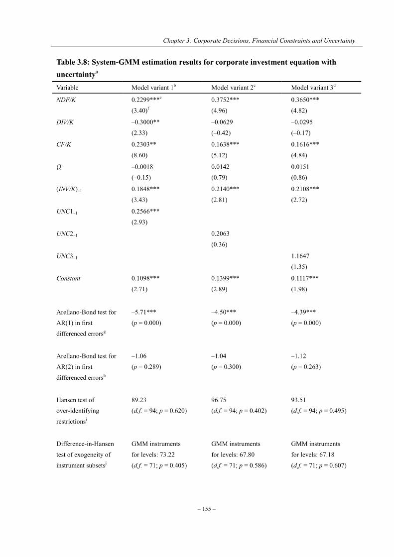
Chapter 3: Corporate Decisions, Financial Constraints and Uncertainty
– 155 –
Table 3.8: System-GMM estimation results for corporate investment equation with uncertaintya Variable Model variant 1b Model variant 2c Model variant 3d
NDF/K 0.2299***e (3.40)f
0.3752*** (4.96)
0.3650*** (4.82)
DIV/K –0.3000** (2.33)
–0.0629 (–0.42)
–0.0295 (–0.17)
CF/K 0.2303** (8.60)
0.1638*** (5.12)
0.1616*** (4.84)
Q –0.0018 (–0.15)
0.0142 (0.79)
0.0151 (0.86)
(INV/K)–1 0.1848*** (3.43)
0.2140*** (2.81)
0.2108*** (2.72)
UNC1–1 0.2566*** (2.93)
UNC2–1 0.2063 (0.36)
UNC3–1 1.1647 (1.35)
Constant 0.1098*** (2.71)
0.1399*** (2.89)
0.1117*** (1.98)
Arellano-Bond test for AR(1) in first differenced errorsg
–5.71*** (p = 0.000)
–4.50*** (p = 0.000)
–4.39*** (p = 0.000)
Arellano-Bond test for AR(2) in first differenced errorsh
–1.06 (p = 0.289)
–1.04 (p = 0.300)
–1.12 (p = 0.263)
Hansen test of over-identifying restrictionsi
89.23 (d.f. = 94; p = 0.620)
96.75 (d.f. = 94; p = 0.402)
93.51 (d.f. = 94; p = 0.495)
Difference-in-Hansen test of exogeneity of instrument subsetsj
GMM instruments for levels: 73.22 (d.f. = 71; p = 0.405)
GMM instruments for levels: 67.80 (d.f. = 71; p = 0.586)
GMM instruments for levels: 67.18 (d.f. = 71; p = 0.607)
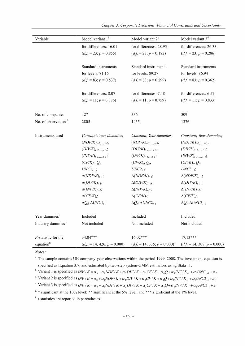
Chapter 3: Corporate Decisions, Financial Constraints and Uncertainty
– 156 –
Variable Model variant 1b Model variant 2c Model variant 3d
for differences: 16.01 (d.f. = 23; p = 0.855) Standard instruments for levels: 81.16 (d.f. = 83; p = 0.537) for differences: 8.07 (d.f. = 11; p = 0.386)
for differences: 28.95 (d.f. = 23; p = 0.182) Standard instruments for levels: 89.27 (d.f. = 83; p = 0.299) for differences: 7.48 (d.f. = 11; p = 0.759)
for differences: 26.33 (d.f. = 23; p = 0.286) Standard instruments for levels: 86.94 (d.f. = 83; p = 0.362) for differences: 6.57 (d.f. = 11; p = 0.833)
No. of companies 427 336 309
No. of observationsk 2805
1435 1376
Instruments used Constant; Year dummies; (NDF/K)t–2,…, t–5; (DIV/K)t–2,…, t–5; (INV/K)t–3,…, t–5; (CF/K)t; Qt; UNC1t–1; ∆(NDF/K)t–1; ∆(DIV/K)t–1; ∆(INV/K)t–2; ∆(CF/K)t; ∆Qt; ∆UNC1t–1
Constant; Year dummies; (NDF/K)t–2,…, t–5; (DIV/K)t–2,…, t–5; (INV/K)t–3,…,t–5; (CF/K)t; Qt; UNC2t–1; ∆(NDF/K)t–1; ∆(DIV/K)t–1; ∆(INV/K)t–2; ∆(CF/K)t; ∆Qt; ∆UNC2t–1
Constant; Year dummies; (NDF/K)t–2,…, t–5; (DIV/K)t–2,…, t–5; (INV/K)t–3,…, t–5; (CF/K)t; Qt; UNC3t–1; ∆(NDF/K)t–1; ∆(DIV/K)t–1; ∆(INV/K)t–2; ∆(CF/K)t; ∆Qt; ∆UNC3t–1
Year dummiesl Included Included Included
Industry dummiesm
Not included Not included Not included
F-statistic for the equationn
34.04*** (d.f. = 14, 426; p = 0.000)
16.02*** (d.f. = 14, 335; p = 0.000)
17.13*** (d.f. = 14, 308; p = 0.000)
Notes: a. The sample contains UK company-year observations within the period 1999–2008. The investment equation is
specified as Equation 3.7, and estimated by two-step system-GMM estimators using Stata 11. b. Variant 1 is specified as 161543210 1///// UNCKINVQKCFKDIVKNDFKINV . c. Variant 2 is specified as 161543210 2///// UNCKINVQKCFKDIVKNDFKINV . d. Variant 3 is specified as 161543210 3///// UNCKINVQKCFKDIVKNDFKINV . e. * significant at the 10% level; ** significant at the 5% level; and *** significant at the 1% level. f. t-statistics are reported in parentheses.

Chapter 3: Corporate Decisions, Financial Constraints and Uncertainty
– 157 –
g. The Arellona-Bond test tests for serial correlation in the first-differenced errors in order to purge the unobserved and perfectly autocorrelated individual effects. Autocorrelation at order 1 is expected in the first differences, because 1 ititit should correlate with 211 ititit , since they share the 1it term.
h. To check for AR(1) in levels, look for AR(2) in differences, in the idea that this will detect the relationship between the 1it in it and the 2it in 2 it . Autocorrelation indicates that lags of the dependent variable (and any other variables used as instruments that are not strictly exogenous), are in fact endogenous, thus bad instruments. Therefore, rejecting the null hypothesis of no serial correlation in the first-differenced errors at an order greater than one implies model misspecification.
i. The Hansen overidentifying restrictions test tests for whether the instruments, as a group, appear exogenous. Under two-step robust GMM estimation, the Sargan statistic is not robust to heteroscedasticity or autocorrelation, but the Hensen J-statistic, which is the minimised value of the two-step GMM criterion function, is robust. The joint null hypothesis is that the instruments are valid instruments, i.e. uncorrelated with the error term, and that the excluded instruments are correctly excluded from the estimated equation. A statistically significant test statistic always indicates that the instruments may not be valid. However, the J-test has its own problem: it can be greatly weakened by instrument proliferation.
j. The difference-in-Hansen test tests for whether subsets of instruments are valid. To be precise, it reports one test for each group of instruments.
k. 2,805 company-year observations are used to estimate model variant 1 in which all the relevant variables are computed using Worldscope data. The number of observation reduced to 1,435 for model variant 2, because UNC2 are derived from daily share returns which are collected from the DataStream database. The merge of the two datasets results in significant decrease in the number of observations. By excluding companies whose stock returns do not exhibit GARCH effect and thus UNC3 cannot be derived, the number of observations further reduces to 1,376 for model variant 3.
l. Year dummies are included in all of the equations to account for the time effect. m. In alternative estimates industry dummies are also included to account for the inter-industry variations. Since
they are jointly insignificant, we ignored them in the final set of estimates. n. F-statistic tests the null hypothesis that all of the coefficients except the intercept coefficient are jointly zero.
Turning to the regression results of model variants 2 and 3 reported in Table 3.8, the
coefficients of the endogenous explanatory variables remain qualitatively unchanged. But the
dividend variables become statistically insignificant at the usual significance levels.
Meanwhile, the supplementary uncertainty measures (i.e. UNC2 and UNC3) are also
insignificant in their respective regressions. However, the estimated coefficients on all of the
uncertainty proxies remain positive. The relatively disappointing explanatory powers of
Chapter 3: Corporate Decisions, Financial Constraints and Uncertainty
– 158 –
UNC2 and UNC3 in the investment model are most likely attributable to the high-frequency
noise contained in the daily stock return observations. Besides, the investment equation
regression results also show that the coefficients on the proxy for Tobin’s Q are insignificant
and inconsistent across the model variants. It is well documented that the low explanatory
power of the Q variable is mainly due to its severe measurement problems. Thus, the poor
performance of the Q variable in our regressions is not contradictory to the usual results from
previous applied studies on corporate investment (see, for example, Lensink and Murinde,
2006). The coefficients on the lagged investment variable, in contrast, are consistently
positive and highly significant in all variants, suggesting that corporate investment behaviour
is indeed a dynamic process, as expected.
Besides, the results of diagnostic tests reported in Table 3.8 also suggest that the
investment model performs reasonably well. Specifically, the results of Arellano-Bond test
show that the first-differenced errors are autocorrelated at order 1, as expected. Meanwhile,
the first-differenced errors are not autocorrelated at order 2, indicating that the model is well
specified. In addition, the results of Hansen overidentifying restrictions test suggest that the
instruments used in the system-GMM estimation are generally valid, both in the
first-differenced and levels equations.
3.6.1.2 Financing equation estimation results
The results for the debt financing equation are presented in Table 3.9. Again, the only
difference across the three model variants is that different uncertainty measures are used in
Chapter 3: Corporate Decisions, Financial Constraints and Uncertainty
– 159 –
their respective regressions. Looking first at the primary results reported in column 2, it is
shown that both the investment (INV/K) and dividend (DIV/K) variables are significant
determinants of external debt financing (NDF/K) as implied by the flow-of-funds framework.
The positive signs of the coefficients on the endogenous explanatory variables suggest that the
level of new debt issued by a company depends primarily on the demand of its investment
outlays and dividend payouts. Additionally, internally generated cash flow (CF/K) as an
alternative source of funds has a significant and negative effect on borrowing. Thus, our
empirical results obtained from the panel of UK-listed companies are entirely in line with the
hierarchy of raising funds as predicted by the pecking order hypotheses. This shows that, in
the presence of information asymmetry, companies rely heavily on their internally generated
funds, while the net amount of debt issued during a fiscal year is chiefly driven by their
financing deficits.
Meanwhile, company size (SZ) is also proved to be an important determinant of new
debt financing. Large companies are typically long-established, diversified, financially
healthy companies with low default risks and good credit ratings, and hence are less likely to
be constrained by access to external finance (see Guariglia, 2008). However, the coefficient
on the asset tangibility variable (TAN) turns out to be significant but negative. This finding is
contrary to the intuition that tangible assets, such as property, plant and equipment, can be
easily valued by outsiders and used as collateral for loans, which is supposed to increase a
company’s borrowing capacity.
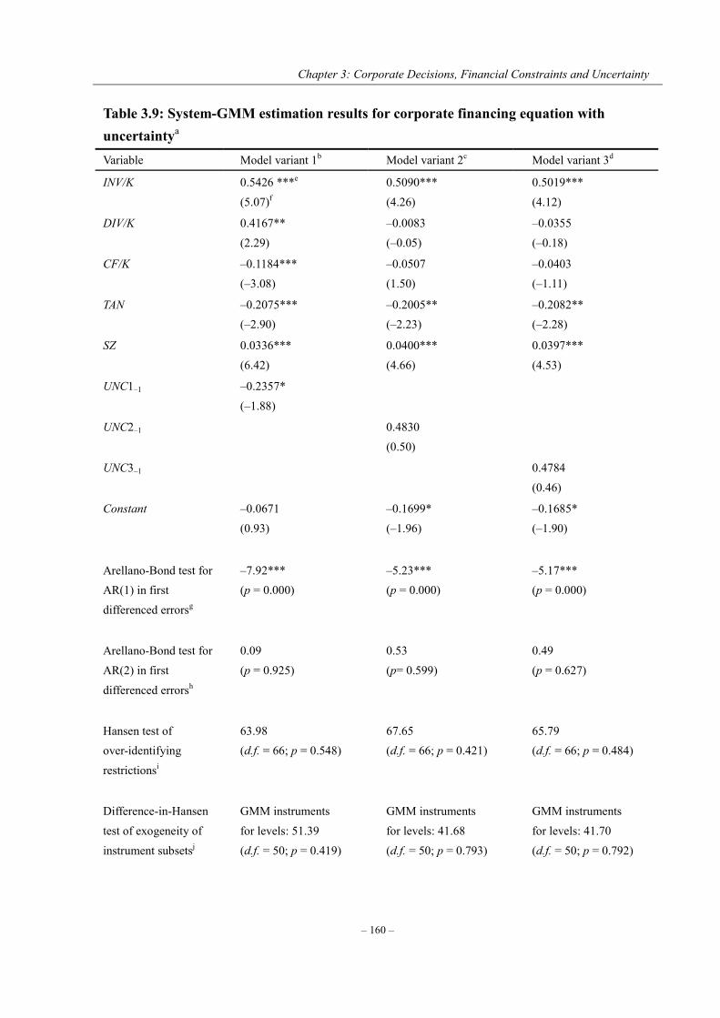
Chapter 3: Corporate Decisions, Financial Constraints and Uncertainty
– 160 –
Table 3.9: System-GMM estimation results for corporate financing equation with uncertaintya Variable Model variant 1b Model variant 2c Model variant 3d
INV/K 0.5426 ***e (5.07)f
0.5090*** (4.26)
0.5019*** (4.12)
DIV/K 0.4167** (2.29)
–0.0083 (–0.05)
–0.0355 (–0.18)
CF/K –0.1184*** (–3.08)
–0.0507 (1.50)
–0.0403 (–1.11)
TAN –0.2075*** (–2.90)
–0.2005** (–2.23)
–0.2082** (–2.28)
SZ 0.0336*** (6.42)
0.0400*** (4.66)
0.0397*** (4.53)
UNC1–1 –0.2357* (–1.88)
UNC2–1 0.4830 (0.50)
UNC3–1 0.4784 (0.46)
Constant –0.0671 (0.93)
–0.1699* (–1.96)
–0.1685* (–1.90)
Arellano-Bond test for AR(1) in first differenced errorsg
–7.92*** (p = 0.000)
–5.23*** (p = 0.000)
–5.17*** (p = 0.000)
Arellano-Bond test for AR(2) in first differenced errorsh
0.09 (p = 0.925)
0.53 (p= 0.599)
0.49 (p = 0.627)
Hansen test of over-identifying restrictionsi
63.98 (d.f. = 66; p = 0.548)
67.65 (d.f. = 66; p = 0.421)
65.79 (d.f. = 66; p = 0.484)
Difference-in-Hansen test of exogeneity of instrument subsetsj
GMM instruments for levels: 51.39 (d.f. = 50; p = 0.419)
GMM instruments for levels: 41.68 (d.f. = 50; p = 0.793)
GMM instruments for levels: 41.70 (d.f. = 50; p = 0.792)
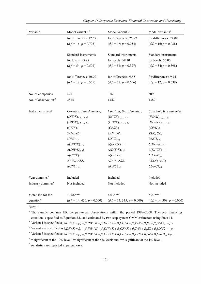
Chapter 3: Corporate Decisions, Financial Constraints and Uncertainty
– 161 –
Variable Model variant 1b Model variant 2c Model variant 3d
for differences: 12.59 (d.f. = 16; p = 0.703) Standard instruments for levels: 53.28 (d.f. = 54; p = 0.502) for differences: 10.70 (d.f. = 12; p = 0.555)
for differences: 25.97 (d.f. = 16; p = 0.054) Standard instruments for levels: 58.10 (d.f. = 54; p = 0.327) for differences: 9.55 (d.f. = 12; p = 0.656)
for differences: 24.09 (d.f. = 16; p = 0.088) Standard instruments for levels: 56.05 (d.f. = 54; p = 0.398) for differences: 9.74 (d.f. = 12; p = 0.639)
No. of companies 427 336 309
No. of observationsk
2814 1442 1382
Instruments used Constant; Year dummies; (INV/K)t–2,..., t–5; (DIV/K)t–2,..., t–5; (CF/K)t; TANt; SZt; UNC1t–1; ∆(INV/K)t–1; ∆(DIV/K)t–1; ∆(CF/K)t; ∆TANt; ∆SZt; ∆UNC1t–1
Constant; Year dummies; (INV/K)t–2,..., t–5; (DIV/K)t–2,..., t–5; (CF/K)t; TANt; SZt; UNC2t–1; ∆(INV/K)t–1; ∆(DIV/K)t–1; ∆(CF/K)t; ∆TANt; ∆SZt; ∆UNC2t–1
Constant; Year dummies; (INV/K)t–2,..., t–5; (DIV/K)t–2,..., t–5; (CF/K)t; TANt; SZt; UNC3t–1; ∆(INV/K)t–1; ∆(DIV/K)t–1; ∆(CF/K)t; ∆TANt; ∆SZt; ∆UNC3t–1
Year dummiesl Included Included Included
Industry dummiesm
Not included Not included Not included
F-statistic for the equationn
10.66*** (d.f. = 14, 426; p = 0.000)
6.03*** (d.f. = 14, 335; p = 0.000)
5.29*** (d.f. = 14, 308; p = 0.000)
Notes: a. The sample contains UK company-year observations within the period 1999–2008. The debt financing
equation is specified as Equation 3.8, and estimated by two-step system-GMM estimators using Stata 11. b. Variant 1 is specified as 16543210 1//// UNCSZTANKCFKDIVKINVKNDF . c. Variant 2 is specified as 16543210 2//// UNCSZTANKCFKDIVKINVKNDF . d. Variant 3 is specified as 16543210 3//// UNCSZTANKCFKDIVKINVKNDF . e. * significant at the 10% level; ** significant at the 5% level; and *** significant at the 1% level. f. t-statistics are reported in parentheses.
Chapter 3: Corporate Decisions, Financial Constraints and Uncertainty
– 162 –
g. The Arellona-Bond test tests for serial correlation in the first-differenced errors in order to purge the unobserved and perfectly autocorrelated individual effects. Autocorrelation at order 1 is expected in the first differences, because 1 ititit should correlate with 211 ititit , since they share the 1it term.
h. To check for AR(1) in levels, look for AR(2) in differences, in the idea that this will detect the relationship between the 1it in it and the 2it in 2 it . Autocorrelation indicates that lags of the dependent variable (and any other variables used as instruments that are not strictly exogenous), are in fact endogenous, thus bad instruments. Therefore, rejecting the null hypothesis of no serial correlation in the first-differenced errors at an order greater than one implies model misspecification.
i. The Hansen overidentifying restrictions test tests for whether the instruments, as a group, appear exogenous. Under two-step robust GMM estimation, the Sargan statistic is not robust to heteroscedasticity or autocorrelation, but the Hensen J-statistic, which is the minimised value of the two-step GMM criterion function, is robust. The joint null hypothesis is that the instruments are valid instruments, i.e. uncorrelated with the error term, and that the excluded instruments are correctly excluded from the estimated equation. A statistically significant test statistic always indicates that the instruments may not be valid. However, the J-test has its own problem: it can be greatly weakened by instrument proliferation.
j. The difference-in-Hansen test tests for whether subsets of instruments are valid. To be precise, it reports one test for each group of instruments.
k. 2,814 company-year observations are used to estimate model variant 1 in which all the relevant variables are computed using Worldscope data. The number of observation reduced to 1,442 for model variant 2, because UNC2 are derived from daily share returns which are collected from the DataStream database. The merge of the two datasets results in significant decrease in the number of observations. By excluding companies whose stock returns do not exhibit GARCH effect and thus UNC3 cannot be derived, the number of observations further reduces to 1,382 for model variant 3.
l. Year dummies are included in all of the equations to account for the time effect. m. In alternative estimates industry dummies are also included to account for the inter-industry variations. Since
they are jointly insignificant, we ignored them in the final set of estimates. n. F-statistic tests the null hypothesis that all of the coefficients except the intercept coefficient are jointly zero.
Finally, the effect of uncertainty on external debt financing is negative and significant
at the 10% level according to the primary results. This is in line with our hypothesis that
greater uncertainty may exacerbate the degree of information asymmetry which in turn
exaggerates the cost disadvantage of debt or even results in credit rationing, reducing the
availability of external financing.
The results for the other two model variants are also reported in Table 3.9. The results
Chapter 3: Corporate Decisions, Financial Constraints and Uncertainty
– 163 –
show that, among the set of potential determinants of companies’ borrowing decisions, only
the investment and company size variables are uniformly and highly significant across all
model variants. This indicates that investment demand and access to external finance are the
most reliably important factors in the external debt financing decisions of UK-listed
companies. The impacts of the dividend, cash flow and uncertainty variables turn into
insignificant in model variants 2 and 3. The diminished explanatory power of the dividend
variable may imply that companies are less likely to fund their desired dividend payouts by
resorting to external finance.
Besides, the results of diagnostic tests suggest that the specification of the debt
financing equation is reasonably well, and that the instruments used in the system-GMM
estimation are generally valid.
3.6.1.3 Dividend equation estimation results
Turing to the dividend equation, the estimation results are presented in Table 3.10. Among the
potential determinants, the cash flow variable (CF/K) has the greatest impact on dividend
decisions. The coefficient on CF/K is consistently positive and highly significant throughout
all model variants. Thus the signalling hypothesis of dividends under information asymmetry
is empirically supported by our sample, which means that managers in UK-listed companies
signal their private knowledge about the distributional support of the project cash flow to the
market through their choice of dividends.
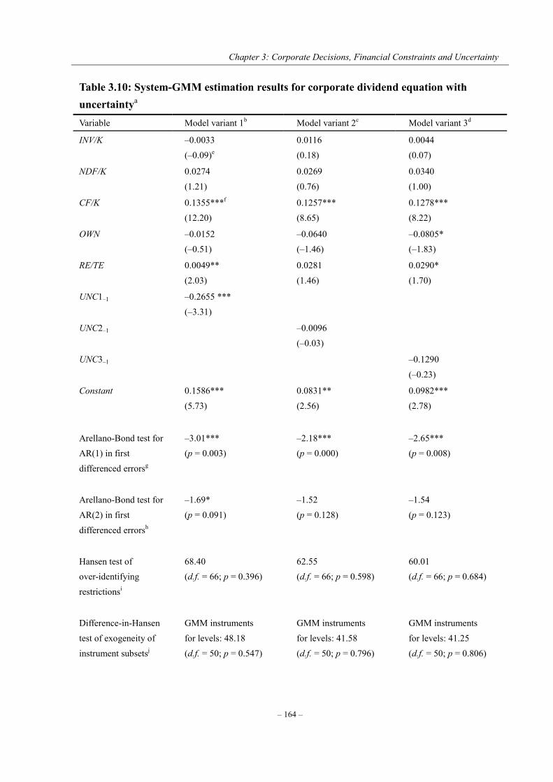
Chapter 3: Corporate Decisions, Financial Constraints and Uncertainty
– 164 –
Table 3.10: System-GMM estimation results for corporate dividend equation with uncertaintya Variable Model variant 1b Model variant 2c Model variant 3d
INV/K –0.0033 (–0.09)e
0.0116 (0.18)
0.0044 (0.07)
NDF/K 0.0274 (1.21)
0.0269 (0.76)
0.0340 (1.00)
CF/K 0.1355***f (12.20)
0.1257*** (8.65)
0.1278*** (8.22)
OWN –0.0152 (–0.51)
–0.0640 (–1.46)
–0.0805* (–1.83)
RE/TE 0.0049** (2.03)
0.0281 (1.46)
0.0290* (1.70)
UNC1–1 –0.2655 *** (–3.31)
UNC2–1 –0.0096 (–0.03)
UNC3–1 –0.1290 (–0.23)
Constant 0.1586*** (5.73)
0.0831** (2.56)
0.0982*** (2.78)
Arellano-Bond test for AR(1) in first differenced errorsg
–3.01*** (p = 0.003)
–2.18*** (p = 0.000)
–2.65*** (p = 0.008)
Arellano-Bond test for AR(2) in first differenced errorsh
–1.69* (p = 0.091)
–1.52 (p = 0.128)
–1.54 (p = 0.123)
Hansen test of over-identifying restrictionsi
68.40 (d.f. = 66; p = 0.396)
62.55 (d.f. = 66; p = 0.598)
60.01 (d.f. = 66; p = 0.684)
Difference-in-Hansen test of exogeneity of instrument subsetsj
GMM instruments for levels: 48.18 (d.f. = 50; p = 0.547)
GMM instruments for levels: 41.58 (d.f. = 50; p = 0.796)
GMM instruments for levels: 41.25 (d.f. = 50; p = 0.806)
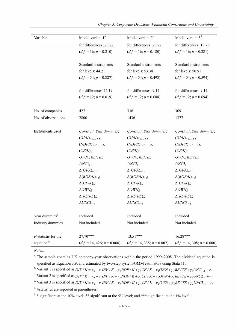
Chapter 3: Corporate Decisions, Financial Constraints and Uncertainty
– 165 –
Variable Model variant 1b Model variant 2c Model variant 3d
for differences: 20.22 (d.f. = 16; p = 0.210) Standard instruments for levels: 44.21 (d.f. = 54; p = 0.827) for differences:24.19 (d.f. = 12; p = 0.019)
for differences: 20.97 (d.f. = 16; p = 0.180) Standard instruments for levels: 53.38 (d.f. = 54; p = 0.498) for differences: 9.17 (d.f. = 12; p = 0.688)
for differences: 18.76 (d.f. = 16; p = 0.281) Standard instruments for levels: 50.91 (d.f. = 54; p = 0.594) for differences: 9.11 (d.f. = 12; p = 0.694)
No. of companies 427 336 309
No. of observations
2800 1436 1377
Instruments used Constant; Year dummies; (GI/K)t–2,..., t–5; (NDF/K)t–2,..., t–5; (CF/K)t; OWNt; RE/TEt; UNC1t–1;
∆(GI/K)t–1;
∆(BOR/K)t–1;
∆(CF/K)t; ∆OWNt; ∆(RE/BE)t; ∆UNC1t–1
Constant; Year dummies; (GI/K)t–2,..., t–5; (NDF/K)t–2,..., t–5; (CF/K)t; OWNt; RE/TEt; UNC2t–1;
∆(GI/K)t–1;
∆(BOR/K)t–1;
∆(CF/K)t; ∆OWNt; ∆(RE/BE)t; ∆UNC2t–1
Constant; Year dummies; (GI/K)t–2,..., t–5; (NDF/K)t–2,..., t–5; (CF/K)t; OWNt; RE/TEt; UNC3t–1;
∆(GI/K)t–1;
∆(BOR/K)t–1;
∆(CF/K)t; ∆OWNt; ∆(RE/BE)t; ∆UNC3t–1
Year dummiesk Included Included Included
Industry dummiesl
Not included Not included Not included
F-statistic for the equationm
27.70*** (d.f. = 14, 426; p = 0.000)
13.51*** (d.f. = 14, 335; p = 0.002)
16.28*** (d.f. = 14, 308; p = 0.000)
Notes: a. The sample contains UK company-year observations within the period 1999–2008. The dividend equation is
specified as Equation 3.9, and estimated by two-step system-GMM estimators using Stata 11. b. Variant 1 is specified as 16543210 1///// UNCTEREOWNKCFKNDFKINVKDIV . c. Variant 2 is specified as 16543210 2///// UNCTEREOWNKCFKNDFKINVKDIV . d. Variant 3 is specified as 16543210 3///// UNCTEREOWNKCFKNDFKINVKDIV . e. t-statistics are reported in parentheses. f. * significant at the 10% level; ** significant at the 5% level; and *** significant at the 1% level.
Chapter 3: Corporate Decisions, Financial Constraints and Uncertainty
– 166 –
g. The Arellona-Bond test tests for serial correlation in the first-differenced errors in order to purge the unobserved and perfectly autocorrelated individual effects. Autocorrelation at order 1 is expected in the first differences, because 1 ititit should correlate with 211 ititit , since they share the 1it term.
h. To check for AR(1) in levels, look for AR(2) in differences, in the idea that this will detect the relationship between the 1it in it and the 2it in 2 it . Autocorrelation indicates that lags of the dependent
variable (and any other variables used as instruments that are not strictly exogenous), are in fact endogenous, thus bad instruments. Therefore, rejecting the null hypothesis of no serial correlation in the first-differenced errors at an order greater than one implies model misspecification.
i. The Hansen overidentifying restrictions test tests for whether the instruments, as a group, appear exogenous. Under two-step robust GMM estimation, the Sargan statistic is not robust to heteroscedasticity or autocorrelation, but the Hensen J-statistic, which is the minimised value of the two-step GMM criterion function, is robust. The joint null hypothesis is that the instruments are valid instruments, i.e. uncorrelated with the error term, and that the excluded instruments are correctly excluded from the estimated equation. A statistically significant test statistic always indicates that the instruments may not be valid. However, the J-test has its own problem: it can be greatly weakened by instrument proliferation.
j. The difference-in-Hansen test tests for whether subsets of instruments are valid. To be precise, it reports one test for each group of instruments.
k. 2,800 company-year observations are used to estimate model variant 1 in which all the variables are computed using Worldscope data. The number of observation reduced to 1,436 for model variant 2, because UNC2 are derived from daily share returns which are collected from the DataStream database. The merge of the two datasets results in significant decrease in the number of observations. By excluding companies whose stock returns do not exhibit GARCH effect and thus UNC3 cannot be derived, the number of observations further reduces to 1,377 for model variant 3.
l. Year dummies are included in all of the equations to account for the time effect. m. In alternative estimates, industry dummies are also included to account for the inter-industry variations. Since
they are jointly insignificant, we ignored them in the final set of estimates. n. F-statistic tests the null hypothesis that all of the coefficients except the intercept coefficient are jointly zero.
The coefficients on the two endogenous explanatory variables (INV/K and NDF/K),
however, are not statistically significant in the dividend regression even though both of them
bear the expected signs, as the flow-of-funds framework predicted, in model variant 1 where
the primary measure of uncertainty is used. Given the significant impact of dividends on
investment decision and the insignificant impact of investment on dividend decisions, it
seems that, if the availability of funds is not sufficient to allow independence between
Chapter 3: Corporate Decisions, Financial Constraints and Uncertainty
– 167 –
investment and dividend policies, UK-listed companies give dividends priority over
investment. This leaves doubt as to whether dividend policy is independent of or
interdependent with investment and financing choices.
As for the exogenous variables in the payout regression, insider ownership (OWN)
does not seem to perform well as a determinant of dividend payouts, but the consistently
negative coefficients associated with it to some extent indicate that insider holding of the
common shares reduces the need for dividends as a monitoring mechanism and then reduces
the dividend payout. Compared with insider ownership, the companies’ financial life cycle
stage variable (RE/TE) has a more significant impact on dividend decisions. The coefficients
for RE/TE have the predicted positive sign everywhere, suggesting that companies in the
mature life cycle stage tend to pay high dividends.
Again, the results of diagnostic test reported in Table 3.10 suggest that both the model
and the instruments are generally well specified. However, the results of Arellona-Bond test
indicate that the first-differenced errors obtained by estimating model variant 1 are likely to
be autocorrelated at the 10% significance level.
3.6.2 Simultaneous equations analyses
The system-GMM analysis reported above indicates that corporate investment, financing and
payout decisions are likely to be endogenous and sensitive to uncertainty in reality. All of the
coefficients of the right-hand side endogenous variables bear the expected signs, and four out
of six of them are statistically significant. To provide further evidence and more insights into

Chapter 3: Corporate Decisions, Financial Constraints and Uncertainty
– 168 –
the joint determination of the set of corporate decisions under uncertainty, we carry out
simultaneous equations analyses.
Specifically, we estimate Equations 3.7 through 3.9 within a simultaneous equations
system using both the three-stage least squares (3SLS) method and two-stage least squares
(2SLS) method, which explicitly allow for the interdependence of the set of corporate
decisions, while controlling for effects that other factors may have on these decisions. The
structure of the three corporate behaviour equations, i.e. Equations 3.7, 3.8 and 3.9, suggests
that the necessary condition, i.e. the order condition, for identification are satisfied, and thus
the system can be identified.26
To apply the 2SLS to the system of structural equations, the reduced form equations
are estimated by the ordinary least squares method to obtain the fitted values for the
endogenous variables in the first stage. The structural equations, in which the fitted values are
used in place of the right-hand side endogenous variables, are then estimated in the second
stage. Additionally, the 3SLS method provides a third step in the estimation procedure that
allows for non-zero covariances between the error terms across equations. The essential
advantage of the 3SLS estimation technique, therefore, is that it allows not only for
simultaneity among the set of corporate decisions, but also for correlations among the error
components. Thus, it is believed that 3SLS estimators are asymptotically more efficient.
26 Brooks (2008) explains the condition that could be examined to determine whether a given equation from a system is identified. Let G denote the number of structural equations in a simultaneous system. If the number of all endogenous and exogenous variables that are not presented in an equation is G–1, then the equation is just identified. If more than G–1 variables are not presented, then the equation is over-identified. If less than G–1 variables are not presented, then the equation is not identified.
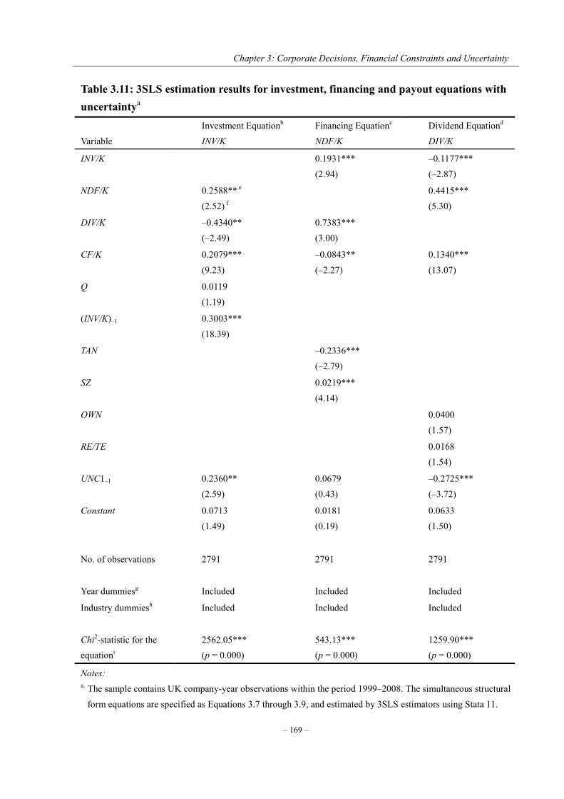
Chapter 3: Corporate Decisions, Financial Constraints and Uncertainty
– 169 –
Table 3.11: 3SLS estimation results for investment, financing and payout equations with uncertaintya
Variable Investment Equationb INV/K
Financing Equationc NDF/K
Dividend Equationd DIV/K
INV/K 0.1931*** (2.94)
–0.1177*** (–2.87)
NDF/K 0.2588** e (2.52) f
0.4415*** (5.30)
DIV/K –0.4340** (–2.49)
0.7383*** (3.00)
CF/K 0.2079*** (9.23)
–0.0843** (–2.27)
0.1340*** (13.07)
Q 0.0119 (1.19)
(INV/K)–1 0.3003*** (18.39)
TAN –0.2336*** (–2.79)
SZ 0.0219*** (4.14)
OWN 0.0400 (1.57)
RE/TE 0.0168 (1.54)
UNC1–1 0.2360** (2.59)
0.0679 (0.43)
–0.2725*** (–3.72)
Constant 0.0713 (1.49)
0.0181 (0.19)
0.0633 (1.50)
No. of observations
2791 2791 2791
Year dummiesg Included Included Included
Industry dummiesh
Included Included Included
Chi2-statistic for the equationi
2562.05*** (p = 0.000)
543.13*** (p = 0.000)
1259.90*** (p = 0.000)
Notes: a. The sample contains UK company-year observations within the period 1999–2008. The simultaneous structural
form equations are specified as Equations 3.7 through 3.9, and estimated by 3SLS estimators using Stata 11.

Chapter 3: Corporate Decisions, Financial Constraints and Uncertainty
– 170 –
b. Investment equation is specified as 161543210 1///// UNCKINVQKCFKDIVKNDFKINV .
c. Financing equation is specified as 16543210 1//// UNCSZTANKCFKDIVKINVKNDF .
d. Dividend equation is specified as 16543210 1///// UNCTEREOWNKCFKNDFKINVKDIV .
e. * significant at the 10% level; ** significant at the 5% level; and *** significant at the 1% level. f. z-statistics are reported in parentheses. g. Year dummies are included in all of the equations to account for the time effect. h. Industry dummies are included in all of the equations to account for the inter-industry variations. i. Chi2-statistic tests the null hypothesis that all of the coefficients except the intercept coefficient are jointly zero.
The panel of UK company-year observations are pooled to gain degrees of freedom.
Both year dummies and industry dummies are included in each equation to account for the
time effect and inter-industry variations that cannot be captured by the included regressors.
Besides, given the relatively disappointing explanatory powers of UNC2 and UNC3 in the
single equation analyses, our empirical findings with respect to the effects of uncertainty on
corporate decisions are drawn from the sign and significance of the coefficients on UNC1 in
the corresponding equations.27
The result from the 3SLS estimation to the system of equations is reported in Table
3.11. Looking first at the investment regression, it suggests that the coefficients of NDF/K and
CF/K are significantly positive as expected, indicating that investments made by UK-listed
companies are likely to be constrained by the availability of internal funds as well as access to
external finance. More importantly, the significant and positive relationship between the
27 3SLS estimation results for corporate investment, financing and payout equations in which UNC2 and UNC3 are used as the proxy for uncertainty are presented in Appendices 3.D and 3.E respectively.
Chapter 3: Corporate Decisions, Financial Constraints and Uncertainty
– 171 –
investment and dividend variables detected in the pair-wise correlation analysis is reversed to
be significant and negative when the full structural investment equation is estimated within
the simultaneous equations system. The negative coefficient of DIV/K is not only statistically
significant but also economically meaningful, suggesting that managers of UK-listed
companies have to trade-off between investment outlays and dividend payouts in order to
allocate scarce funds rationally. Our results lend strong empirical support to the predictions of
the flow-of-funds framework that companies have to consider their financing choices
alongside their investment decisions.
Another result of particular interest is the significant and positive effect of uncertainty
(UNC1) on investment, which is quite robust with respect to the methods of estimation.28 The
positive effect of uncertainty observed from the panel of UK-listed companies critically
challenges the assertion of the established real options theory of investment, but empirically
supports the argument of the recent theoretical innovation by Mason and Weeds (2010). In a
competitive business environment, greater uncertainty may lead companies to invest earlier to
take the advantage of pre-emption, thus the option value of delay investment under
uncertainty is offset by the threat of being pre-empted by their rivals.29 In fact, if the
advantage of pre-emption is sufficiently strong, greater uncertainty can lead to a higher level
of investment even if the projects are irreversible. Besides, the proxy for Tobin’s Q is
28 The system-GMM estimation results for the investment equation show that the coefficient on the proxy for uncertainty is positive and significant at a 1% significance level. 29 Mason and Weeds (2010) show the possibility of pre-emption can have significant qualitative and quantitative effects on the relationship between uncertainty and investment.
Chapter 3: Corporate Decisions, Financial Constraints and Uncertainty
– 172 –
insignificant, although with a positive sign.30 The dynamic structure of corporate investment
is statistically evident.
Turning to the financing regression, the coefficients on the endogenous variables, i.e.
INV/K and DIV/K, are highly significant and uniformly positive, as predicted by the
flow-of-funds framework. It appears that companies’ external debt financing is driven not
only by the demand from capital investment but also by that from dividend payouts. Moreover,
internally generated cash flow (CF/K), as an alternative source of funds, has a significant and
negative effect on the amount of new debt issued in the corresponding period, suggesting that
companies with high levels of cash flow tend to borrow less. These results are entirely
consistent with the predicted hierarchy of raising funds, suggesting that pecking-order
behaviour is rather robust among UK-listed companies. Besides, the effect of company size
(SZ) is highly significant, whilst the effect of asset tangibility (TAN) is also significant but
with a wrong sign. However, the impact of uncertainty on external debt financing is relatively
weak.
Moving to the payout regression, the highly significant coefficients on INV/K and
NDF/K reported in the 3SLS results suggest the importance of investment and financing
choices in the dividends decision-making process. Compared with the statistically
insignificant coefficients on INV/K and NDF/K estimated using system-GMM estimators (see
30 The low explanatory power of Tobin’s Q in investment regression has long been observed in the literature (see, for example, Lensink and Murinde, 2006; Bulan, 2005; and Erickson and Whited, 2000).
Chapter 3: Corporate Decisions, Financial Constraints and Uncertainty
– 173 –
Table 3.10), it seems that the importance of investment and financing choices in the payout
decision-making process is underestimated by the single equation estimation techniques.
Companies with more investment spending and/or less external debt financing tend to pay
less cash dividends. Thus, the simultaneous analysis clearly shows that the dividend decision
is neither totally residual nor totally independent but is taken with reference to investment and
financing decisions. However, the cash flow variable (CF/K) is still the most important
determinant of dividend policy, which implies that UK-listed companies may signal their
anticipated cash flow to the market through their choices of dividend payment. Besides, the
effect of uncertainty (UNC1) on dividend payouts turns out to be negative and highly
significant, lending strong support to our hypothesis that companies facing greater uncertainty
tend to pay less dividends. The results also show that the impact of uncertainty on UK-listed
companies’ payout decisions is statistically more significant and economically more
meaningful than that of other factors which, according to the existing literature, are believed
to be the primary determinants of dividend policy, such as insider ownership (OWN) and
financial life cycle stage (RE/TE). This result implies that investment models that ignore the
dividend payout-uncertainty relationship are likely to produce misleading estimates of the
effect of uncertainty.
To sum up, our results seem to substantiate the claim that corporate investment,
financing and payout decisions are indeed inextricably linked and jointly determined as
implied by the flow-of-funds framework with financial constraints. In addition, companies are

Chapter 3: Corporate Decisions, Financial Constraints and Uncertainty
– 174 –
likely to increase their investment spending in the face of greater uncertainty. To finance the
increased investment under uncertainty, they tend to resort to internal funds by cutting
dividends, rather than resorting to external funds by issuing new debts. These results clearly
support the argument that managers do take uncertainty into consideration when they make
real and financial decisions. Our key findings are summarised in Appendix 3.A.
3.6.3 Long-run solution to the simultaneous equations system
It is useful to note that the coefficient estimates for the simultaneous equations system
reported in Table 3.11 reflect conditional responses, and the conditioning includes the
simultaneously determined corporate decision variables, namely, INV/K, NDF/K and DIV/K.
Given some of the coefficient matrices for the endogenous variables seem to be non-positive,
it cannot be assumed that the solved-out coefficients have the same sign as the conditional
coefficients reported in Table 3.11. The objective of this section, therefore, is to obtain a
long-run solution to the dynamic simultaneous equations system. To this end, we define Y as a
3×1 vector of endogenous corporate decision variables; Z as a 1k vector of exogenous
variables ( 7k , according to the specification of Equations 3.7–3.9), including cash flow,
Tobin’s Q, company size, asset tangibility, insider ownership and financial life cycle stage; A
as a 3×1 vector of constants; B and C as 3×3 matrices of coefficients; and D as a k3
matrix of coefficients.31 The estimated simultaneous equations system, therefore, can be
31 Both the coefficient matrices B and C and the coefficient vector D include zeros depending on the model specification (see Equations 3.7–3.9).

Chapter 3: Corporate Decisions, Financial Constraints and Uncertainty
– 175 –
written using matrix algebra as follows,
tttt DZCYBYAY 1 (3.12)
We further define I as a 3×3 identity matrix. So that the solution for Yt can be written as
follows,
)()( 11
ttt DZCYABIY
(3.13)
Therefore, any long-run static equilibrium solution to the dynamic system can be obtained by
computing the coefficient matrices in the following equation,
DZABICBIIY 111 (3.14)
Time subscripts are removed from the variables because it is assumed that in the long run the
variables attain some steady state values and are no longer changing, i.e. are in equilibrium.
Table 3.12 presents the long-run solution to the simultaneous equations system, which
is computed based on the 3SLS estimates reported in Table 3.11. It is evident that the
solved-out coefficients presented in Table 3.12 are consistent generally with the conditional
coefficients reported in Table 3.12 in terms of their signs and sizes.
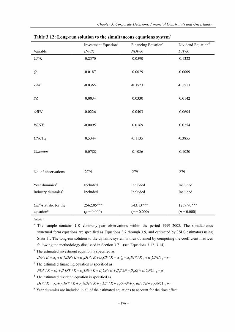
Chapter 3: Corporate Decisions, Financial Constraints and Uncertainty
– 176 –
Table 3.12: Long-run solution to the simultaneous equations systema Variable
Investment Equationb INV/K
Financing Equationc NDF/K
Dividend Equationd DIV/K
CF/K 0.2370
0.0590
0.1322
Q 0.0187
0.0029
-0.0009
TAN -0.0365
-0.3523
-0.1513
SZ 0.0034
0.0330
0.0142
OWN -0.0226
0.0403
0.0604
RE/TE -0.0095
0.0169
0.0254
UNC1–1 0.5344
-0.1135
-0.3855
Constant 0.0788
0.1086
0.1020
No. of observations
2791 2791 2791
Year dummiese Included Included Included
Industry dummiesf
Included Included Included
Chi2-statistic for the equationg
2562.05*** (p = 0.000)
543.13*** (p = 0.000)
1259.90*** (p = 0.000)
Notes: a. The sample contains UK company-year observations within the period 1999–2008. The simultaneous
structural form equations are specified as Equations 3.7 through 3.9, and estimated by 3SLS estimators using Stata 11. The long-run solution to the dynamic system is then obtained by computing the coefficient matrices following the methodology discussed in Section 3.7.1 (see Equations 3.12–3.14).
b. The estimated investment equation is specified as 161543210 1///// UNCKINVQKCFKDIVKNDFKINV .
c. The estimated financing equation is specified as 16543210 1//// UNCSZTANKCFKDIVKINVKNDF .
d. The estimated dividend equation is specified as 16543210 1///// UNCTEREOWNKCFKNDFKINVKDIV .
e. Year dummies are included in all of the estimated equations to account for the time effect.

Chapter 3: Corporate Decisions, Financial Constraints and Uncertainty
– 177 –
f. Industry dummies are included in all of the estimated equations to account for the inter-industry variations. g. Chi2-statistic tests the null hypothesis that all of the estimated coefficients except the intercept coefficient are
jointly zero.
However, the coefficient of the cash flow variables in the financing equation turns out
to be positive, which suggests that, in the long run, internally generated cash flow may
increase a company’s borrowing capacity, allowing the company to take on more debt. The
positive effect of cash flow on corporate debt finance lends support to the trade-off prediction
that profitable companies face lower expected costs of financial distress and find interest tax
shields more valuable, and thus tend to take on more debt. Moreover, the proxy for
uncertainty in the financing equation becomes negative. This finding is more consistent with
our prediction that greater uncertainty is likely to exacerbate the degree of information
asymmetry between insiders and external capital markets, resulting in a more significant cost
disadvantage of external debt financing. It also confirms that companies prefer to finance
increased investment under uncertainty by resorting to internal funds rather than external
funds.
In addition, the long-run solution to the simultaneous equations system presented in
Table 3.12 provides some further insights into the determination of corporate decisions. First,
it shows that Tobin’s Q has a positive effect not only on corporate investment but also on debt
financing, while its effect on dividend payouts is negative. These results are in line with the
previous findings that companies are likely to use more debt and retain more cash flow to
finance variable investment opportunities. Second, company size seems to have positive effect

Chapter 3: Corporate Decisions, Financial Constraints and Uncertainty
– 178 –
on all the three corporate decisions, indicating that larger companies are likely to have more
investments, use more debt and distribute more dividends to their shareholders. Third, the
coefficients on the proxy for financial life cycle stage show that, as a company matures, it
tends to have fewer attractive investment opportunities, better access to external funds and
thus a higher propensity to pay dividends. Besides, the coefficients on the assets tangibility
variables are uniformly negative across all the three corporate behaviour equations, and the
coefficients on the insider ownership variable are positive in both the financing and dividend
equations but negative in the investment equation.
Overall, the long-run solution to the dynamic simultaneous equations system suggests
that the solved-out coefficients have the same sign as the conditional coefficients reported in
Table 3.11, except those on the cash flow and uncertainty variables in the financing equation.
Nevertheless, since the coefficient estimates reported for the simultaneous equations system
throughout the thesis reflect conditional responses, the empirical results presented here should
be interpreted with cautions.
3.7 Robustness tests and further evidence
3.7.1 Robustness tests and results
In order to check the robustness of our main findings, we carry out further estimation and
testing procedures. First, instead of using 3SLS estimators, we re-estimate the simultaneous
equations system using 2SLS estimators. Even though the 3SLS method is asymptotically
Chapter 3: Corporate Decisions, Financial Constraints and Uncertainty
– 179 –
more efficient, it is also more vulnerable to specification errors as compared to limited
information methods, such as 2SLS. Therefore, we apply the 2SLS estimation to the
simultaneous equations system. As reported in Appendix 3.B, the 2SLS regression provides
qualitatively similar results to those from the 3SLS estimation.
Second, we re-specify the simultaneous equations system by excluding the uncertainty
variable. The 3SLS estimation results for the simultaneous equations system without
uncertainty variable are reported in Appendix 3.C. As can be seen, all the endogenous
explanatory variables are statistically significance with expected signs. Therefore, the
simultaneity among corporate investment, financing and payout decisions remain hold, in the
absence of the proxy for uncertainty associated with companies’ future prospects.
Third, to determine the sensitivity of our findings to the choice of uncertainty
measurement, we also estimate simultaneous equations systems in which the alternative
measures of uncertainty, i.e. UNC2 and UNC3, are utilised. The 3SLS estimation results are
presented in Appendices 3.D and 3.E, respectively. As expected, the alternative measures of
uncertainty derived from daily stock returns are insignificant in their respective system
variants. The disappointing explanatory power of the alternative measures of uncertainty is
largely attributable to the high-frequency noise contained in the daily stock returns.
Overall, the robustness test results suggest that the corporate behavioural equations
system performs reasonably well. The simultaneity among corporate decisions is robust with
respect to different estimation techniques and model specifications. However, the results

Chapter 3: Corporate Decisions, Financial Constraints and Uncertainty
– 180 –
regarding the effect of uncertainty on corporate decisions are, to some extent, sensitive to how
uncertainty is empirically captured.
3.7.2 Further evidence on the simultaneity of corporate decisions
Furthermore, in an attempt to explicitly explore the possible mechanism through which the set
of corporate decisions are jointly determined, we split the whole sample into two subsamples
based on the financial leverage index (FLI), which is defined as the ratio of return on average
assets to return on average equity and used as a proxy for company’s financial position.32 It is
believed that companies with a lower financial leverage index are highly indebted and hence
more financially constrained, while companies with a higher financial leverage index are less
indebted and hence less financially constrained. The median value of financial leverage index
is used to divide the sample into two subsamples. Those with a lower financial leverage index
are classified as financially more constrained companies, and those with a higher financial
leverage index are financially less constrained companies.33 Given the argument that the joint
determination of corporate decisions is justified by the financial constrains caused by
information asymmetry, the interactions among the set of corporate decisions are expected to
be more pronounced for companies that are financially more constrained than for those that
are financially less constrained. If this is the case, then the financial constraints may be
32 The financial leverage index is collected directly from the Worldscope database via Thomson One Banker Analytics. It is defined as the ratio of return on average assets to return on average equity, which is equivalent to the ratio of average equity to average assets. Therefore, companies with a lower financial leverage index have higher financial leverage, while companies with a higher financial leverage index have lower financial leverage. 33 Our sample split focuses on company-year observations rather than simply companies, and hence allows companies to transit between the two classes. See Guariglia (2008) for a similar approach.
Chapter 3: Corporate Decisions, Financial Constraints and Uncertainty
– 181 –
viewed as the possible channel through which corporate investment, financing and payout
decisions are jointly determined by management.
Panel A of Table 3.13 reports the 3SLS estimation results for the financially more
constrained companies. As expected, companies which are financially more constrained
exhibit much stronger simultaneity among the set of corporate decisions than the full sample
results presented earlier. More specifically, the magnitude of the coefficient on dividend
payout variable in investment equation increases considerably from –0.434 observed from the
full sample results to –1.266 observed from the results for the financially more constrained
group, suggesting that investment and dividends are extremely competitive in financially
more constrained companies. This is also evident from the coefficient on the investment
variable in the payout equation whose magnitude increases significantly from –0.118 to
–0.223. Moreover, the magnitudes of the coefficients on external debt financing and internal
cash flow variables in the investment regression increase from 0.259 and 0.208 to 0.533 and
0.405, respectively. These results are consistent with the well-documented phenomenon that
the sensitivities of investment expenditures to internal cash flows and external debt finance
are higher for financially more constrained companies. In addition, the effects of uncertainty
on investment and payout decisions turn out to be insignificant, whilst the effect of
uncertainty on debt financing becomes negative and marginally significant. It seems that
financially more constrained companies act more defensively under uncertain circumstances,
which may be due to the limited managerial flexibility caused by financial constraints.
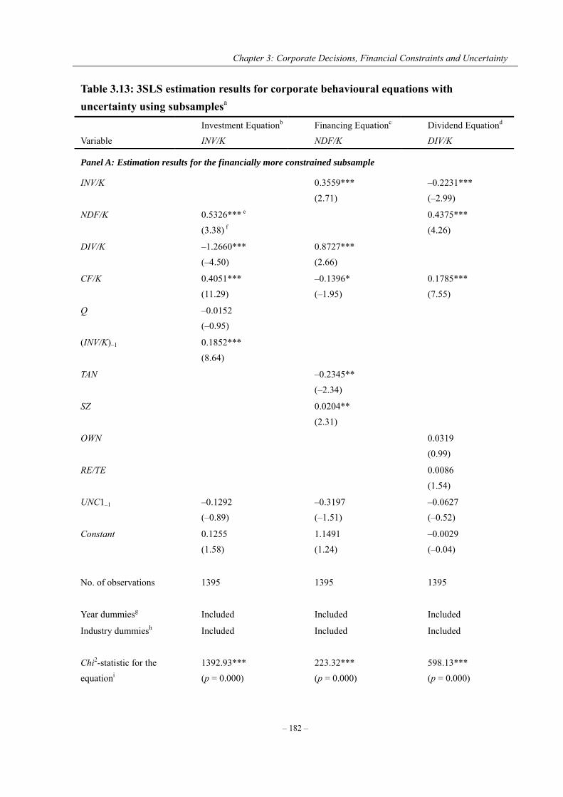
Chapter 3: Corporate Decisions, Financial Constraints and Uncertainty
– 182 –
Table 3.13: 3SLS estimation results for corporate behavioural equations with uncertainty using subsamplesa
Variable Investment Equationb INV/K
Financing Equationc NDF/K
Dividend Equationd DIV/K
Panel A: Estimation results for the financially more constrained subsample
INV/K 0.3559*** (2.71)
–0.2231*** (–2.99)
NDF/K 0.5326*** e (3.38) f
0.4375*** (4.26)
DIV/K –1.2660*** (–4.50)
0.8727*** (2.66)
CF/K 0.4051*** (11.29)
–0.1396* (–1.95)
0.1785*** (7.55)
Q –0.0152 (–0.95)
(INV/K)–1 0.1852*** (8.64)
TAN –0.2345** (–2.34)
SZ 0.0204** (2.31)
OWN 0.0319 (0.99)
RE/TE 0.0086 (1.54)
UNC1–1 –0.1292 (–0.89)
–0.3197 (–1.51)
–0.0627 (–0.52)
Constant 0.1255 (1.58)
1.1491 (1.24)
–0.0029 (–0.04)
No. of observations
1395 1395 1395
Year dummiesg Included Included Included
Industry dummiesh
Included Included Included
Chi2-statistic for the equationi
1392.93*** (p = 0.000)
223.32*** (p = 0.000)
598.13*** (p = 0.000)
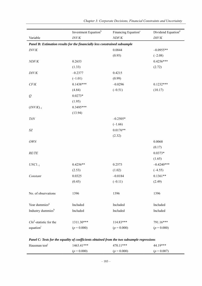
Chapter 3: Corporate Decisions, Financial Constraints and Uncertainty
– 183 –
Variable Investment Equationb INV/K
Financing Equationc NDF/K
Dividend Equationd DIV/K
Panel B: Estimation results for the financially less constrained subsample
INV/K 0.0844 (0.95)
–0.0955** (–2.08)
NDF/K 0.2653 (1.33)
0.4256*** (2.72)
DIV/K –0.2377 (–1.01)
0.4215 (0.99)
CF/K 0.1438*** (4.84)
–0.0296 (–0.51)
0.1232*** (10.17)
Q 0.0273* (1.95)
(INV/K)–1 0.3495*** (13.94)
TAN –0.2505* (–1.66)
SZ 0.0176** (2.32)
OWN 0.0068 (0.17)
RE/TE 0.0373* (1.65)
UNC1–1 0.4256** (2.53)
0.2573 (1.02)
–0.4240*** (–4.55)
Constant 0.0325 (0.45)
–0.0184 (–0.11)
0.1361** (2.49)
No. of observations
1396 1396 1396
Year dummiesg Included Included Included
Industry dummiesh
Included Included Included
Chi2-statistic for the equationi
1311.30*** (p = 0.000)
114.83*** (p = 0.000)
791.16*** (p = 0.000)
Panel C: Tests for the equality of coefficients obtained from the two subsample regressions
Hausman testj 1463.41*** (p = 0.000)
470.11*** (p = 0.000)
44.19*** (p = 0.007)
Chapter 3: Corporate Decisions, Financial Constraints and Uncertainty
– 184 –
Notes: a. Those with lower than median financial leverage index (0.43) are classified as financially more constrained,
and those with higher than median financial leverage index are classified as financially less constrained. The simultaneous structural form equations are specified as Equations 3.7 through 3.9, and estimated by 3SLS estimators using Stata 11.
b. Investment equation is specified as 161543210 1///// UNCKINVQKCFKDIVKNDFKINV .
c. Financing equation is specified as 16543210 1//// UNCSZTANKCFKDIVKINVKNDF .
d. Dividend equation is specified as 16543210 1///// UNCTEREOWNKCFKNDFKINVKDIV .
e. * significant at the 10% level; ** significant at the 5% level; and *** significant at the 1% level. f. z-statistics are reported in parentheses. g. Year dummies are included in all of the equations to account for the time effect. h. Industry dummies are included in all of the equations to account for the inter-industry variations. i. Chi2-statistic tests the null hypothesis that all of the coefficients except the intercept coefficient are jointly zero. j. The Hausman test tests for the equality of the coefficients obtained using different subsamples. The null
hypothesis is that difference in coefficients obtained from two subsample estimations is not systematic. The
test statistic follows a Chi-squared distribution. The associated p-value is reported in parenthesis.
Panel B of Table 3.13 reports the 3SLS estimation for the companies that are
financially less constrained. It shows that, although all the endogenous variables still bear the
expected signs, their explanatory powers decline considerably, with 4 out 6 being statistically
insignificant. Overall, the magnitude of the coefficients on the endogenous variables reduces
significantly, suggesting that the simultaneity among the set of corporate decisions is
relatively weak for financially less constrained companies. Corporate investment decisions of
financially less constrained companies are likely to be independent of their debt financing and
dividend payout decisions, and are less subject to internally generated cash flow as well. The
proxy for Tobin’s Q turns out to be positive and significant, which means that capital
expenditure of financially less constrained companies depends relatively more on the real

Chapter 3: Corporate Decisions, Financial Constraints and Uncertainty
– 185 –
considerations and less on the financial considerations, leading to more efficient investment
decisions. However, the effect of investment on payout decisions remains negative and
significant, which implies that if the available funds are not sufficient to allow independence
between investment and dividend decisions, financially less constrained companies give
investment expenditure priority over dividend payouts. Besides, it is worth noting that the
effects of uncertainty on investment and payout decisions turns out to be statistically
significant at the 5% and 1% levels, respectively. This shows that companies which are
financially less constrained tend to act more aggressively under greater uncertainty, i.e. invest
more and payout less. Presumably, they are more able and more willing to take the advantage
of pre-emption in a competitive business environment by investing earlier, even if the
prospects are not clear. Managers of financially less constrained companies have more
flexibility to raise funds either externally by issuing debt or internally by cutting dividends.
In an attempt to formally test the difference in the results for the two subsamples, we
carry out a Hausman test for each of the corporate behaviour equations. Under the null
hypothesis, the coefficients estimated using financially more constrained companies are not
systematically different from those estimated using financially less constrained companies.
The test results reported in Panel C of Table 3.13 suggest that the null hypothesis of no
substantial difference between the results reported in Panel A and those reported in Panel B
should be resoundingly rejected with respect to all of the corporate behaviour equations.
Therefore, financially more constrained companies indeed behave differently from those

Chapter 3: Corporate Decisions, Financial Constraints and Uncertainty
– 186 –
which are financially less constrained. The keys findings of this chapter are summarised in
Appendix 3.A, alongside the findings from prior research.
3.8 Concluding remarks
In this chapter, we investigate the interactions among corporate investment, financing and
payout decisions under financial constraints and uncertainty, using a large panel of UK-listed
companies. The three main aspects of corporate behaviour are modelled within a simultaneous
equations system where they are treated as endogenous.
On the whole, our results suggest that corporate investment, financing and payout
decisions made by UK-listed companies are indeed inextricably linked and jointly determined
as implied by the flow-of-funds framework, and the simultaneity among them is quite robust
with respect to different methods of estimation. UK-listed companies are likely to be
financially constrained by the availability of internal funds as well as by access to external
finance. Therefore, managers have to consider their financing and payout choices alongside
their investment decisions.
We also find that the effect of uncertainty on corporate investment is positive and
significant, while that on dividend payouts is negative and also significant, suggesting that
uncertainty stimulates investment in our sample not only on its own but also through its effect
on dividend payout policy. Accordingly, companies facing greater uncertainty appear to invest
more, and fund the increased investment spending by resorting to internal finance by cutting
dividends rather than resorting to external finance by issuing new debts.
Chapter 3: Corporate Decisions, Financial Constraints and Uncertainty
– 187 –
Furthermore, we divide the entire sample into financially more constrained and less
constrained subsamples, in order to provide further insights into the simultaneity of corporate
decisions. Comparing the magnitude and significance level of coefficients on the endogenous
variables between the two subsample results, we find that the simultaneity among the
corporate decisions is more pronounced for more constrained companies, whist that for less
constrained companies is relatively weak. Accordingly, we argue that the substantial
economic interactions among the set of corporate decisions observed from UK-listed
companies are likely to be caused by financial constraints.
The subsample regressions also show that the effect of uncertainty is more significant
for financially less constrained companies but insignificant for more constrained companies,
suggesting that less constrained companies respond to uncertainty more aggressively than
more constrained ones. Therefore, our results offer new insight that financial constraints
intensify the simultaneity among corporate investment, financing and payout decisions, and
reduce managerial flexibility in adjusting those corporate decisions in response to uncertainty.
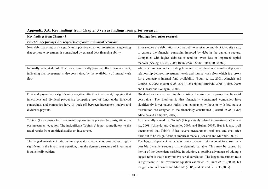
– 188 –
Appendix 3.A: Key findings from Chapter 3 versus findings from prior research Key findings from Chapter 3 Findings from prior research
Panel A: Key findings with respect to corporate investment behaviour
New debt financing has a significantly positive effect on investment, suggesting that corporate investment is constrained by external debt financing ability.
Prior studies use debt ratios, such as debt to asset ratio and debt to equity ratio, to capture the financial constraint imposed by debt in the capital structure. Companies with higher debt ratios tend to invest less in imperfect capital markets (Ascioglu et al., 2008; Baum et al., 2008; Bulan, 2005; etc.).
Internally generated cash flow has a significantly positive effect on investment, indicating that investment is also constrained by the availability of internal cash flow.
Abroad consensus in the existing literature is that there is a significant positive relationship between investment levels and internal cash flow which is a proxy for a company’s internal fund availability (Baum et al., 2008; Almeida and Campello, 2007; Bloom et al., 2007; Lensink and Murinde, 2006; Bulan, 2005; and Ghosal and Loungani, 2000).
Dividend payout has a significantly negative effect on investment, implying that investment and dividend payout are competing uses of funds under financial constraints, and companies have to trade-off between investment outlays and dividends payouts.
Dividend ratios are used in the existing literature as a proxy for financial constraints. The intuition is that financially constrained companies have significantly lower payout ratios, thus companies without or with low payout distribution are assigned to the financially constrained (Fazzari et al., 1988; Almeida and Campello, 2007).
Tobin’s Q as a proxy for investment opportunity is positive but insignificant in our investment equation. The insignificant Tobin’s Q is not contradictory to the usual results from empirical studies on investment.
It is generally agreed that Tobin’s Q is positively related to investment (Baum et al., 2008; Almeida and Campello, 2007; and Bulan, 2005). But it is also well documented that Tobin’s Q has severe measurement problems and thus often turns out to be insignificant in empirical models (Lensink and Murinde, 2006).
The lagged investment ratio as an explanatory variable is positive and highly significant in the investment equation, thus the dynamic structure of investment is statistically evident.
The lagged dependent variable is basically taken into account to allow for a possible dynamic structure in the dynamic variable. This may be caused by inertia of the dependent variable. In addition, a possible advantage of adding a lagged term is that it may remove serial correlation. The lagged investment ratio is significant in the investment equation estimated in Baum et al. (2008), but insignificant in Lensink and Murinde (2006) and Bo and Lensink (2005).
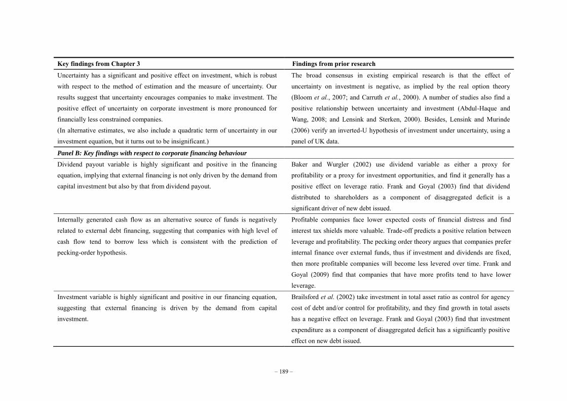
– 189 –
Key findings from Chapter 3 Findings from prior research
Uncertainty has a significant and positive effect on investment, which is robust with respect to the method of estimation and the measure of uncertainty. Our results suggest that uncertainty encourages companies to make investment. The positive effect of uncertainty on corporate investment is more pronounced for financially less constrained companies. (In alternative estimates, we also include a quadratic term of uncertainty in our investment equation, but it turns out to be insignificant.)
The broad consensus in existing empirical research is that the effect of uncertainty on investment is negative, as implied by the real option theory (Bloom et al., 2007; and Carruth et al., 2000). A number of studies also find a positive relationship between uncertainty and investment (Abdul-Haque and Wang, 2008; and Lensink and Sterken, 2000). Besides, Lensink and Murinde (2006) verify an inverted-U hypothesis of investment under uncertainty, using a panel of UK data.
Panel B: Key findings with respect to corporate financing behaviour
Dividend payout variable is highly significant and positive in the financing equation, implying that external financing is not only driven by the demand from capital investment but also by that from dividend payout.
Baker and Wurgler (2002) use dividend variable as either a proxy for profitability or a proxy for investment opportunities, and find it generally has a positive effect on leverage ratio. Frank and Goyal (2003) find that dividend distributed to shareholders as a component of disaggregated deficit is a significant driver of new debt issued.
Internally generated cash flow as an alternative source of funds is negatively related to external debt financing, suggesting that companies with high level of cash flow tend to borrow less which is consistent with the prediction of pecking-order hypothesis.
Profitable companies face lower expected costs of financial distress and find interest tax shields more valuable. Trade-off predicts a positive relation between leverage and profitability. The pecking order theory argues that companies prefer internal finance over external funds, thus if investment and dividends are fixed, then more profitable companies will become less levered over time. Frank and Goyal (2009) find that companies that have more profits tend to have lower leverage.
Investment variable is highly significant and positive in our financing equation, suggesting that external financing is driven by the demand from capital investment.
Brailsford et al. (2002) take investment in total asset ratio as control for agency cost of debt and/or control for profitability, and they find growth in total assets has a negative effect on leverage. Frank and Goyal (2003) find that investment expenditure as a component of disaggregated deficit has a significantly positive effect on new debt issued.
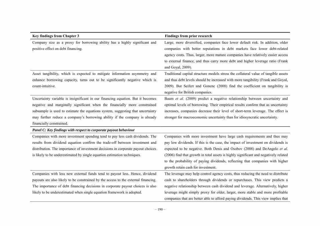
– 190 –
Key findings from Chapter 3 Findings from prior research
Company size as a proxy for borrowing ability has a highly significant and positive effect on debt financing.
Large, more diversified, companies face lower default risk. In addition, older companies with better reputations in debt markets face lower debt-related agency costs. Thus, larger, more mature companies have relatively easier access to external finance, and thus carry more debt and higher leverage ratio (Frank and Goyal, 2009).
Asset tangibility, which is expected to mitigate information asymmetry and enhance borrowing capacity, turns out to be significantly negative which is count-intuitive.
Traditional capital structure models stress the collateral value of tangible assets and thus debt levels should be increased with more tangibility (Frank and Goyal, 2009). But Seifert and Gonenc (2008) find the coefficient on tangibility is negative for British companies.
Uncertainty variable is insignificant in our financing equation. But it becomes negative and marginally significant when the financially more constrained subsample is used to estimate the equations system, suggesting that uncertainty may further reduce a company’s borrowing ability if the company is already financially constrained.
Baum et al. (2009) predict a negative relationship between uncertainty and optimal levels of borrowing. Their empirical results confirm that as uncertainty increases, companies decrease their level of short-term leverage. The effect is stronger for macroeconomic uncertainty than for idiosyncratic uncertainty.
Panel C: Key findings with respect to corporate payout behaviour
Companies with more investment spending tend to pay less cash dividends. The results from dividend equation confirm the trade-off between investment and distribution. The importance of investment decisions in corporate payout choices is likely to be underestimated by single equation estimation techniques.
Companies with more investment have large cash requirements and thus may pay low dividends. If this is the case, the impact of investment on dividends is expected to be negative. Both Denis and Osobov (2008) and DeAngelo et al. (2006) find that growth in total assets is highly significant and negatively related to the probability of paying dividends, reflecting that companies with higher growth retain cash for investment.
Companies with less new external funds tend to payout less. Hence, dividend payouts are also likely to be constrained by the access to the external financing. The importance of debt financing decisions in corporate payout choices is also likely to be underestimated when single equation framework is adopted.
The leverage may help control agency costs, thus reducing the need to distribute cash to shareholders through dividends or repurchases. This view predicts a negative relationship between cash dividend and leverage. Alternatively, higher leverage might simply proxy for older, larger, more stable and more profitable companies that are better able to afford paying dividends. This view implies that
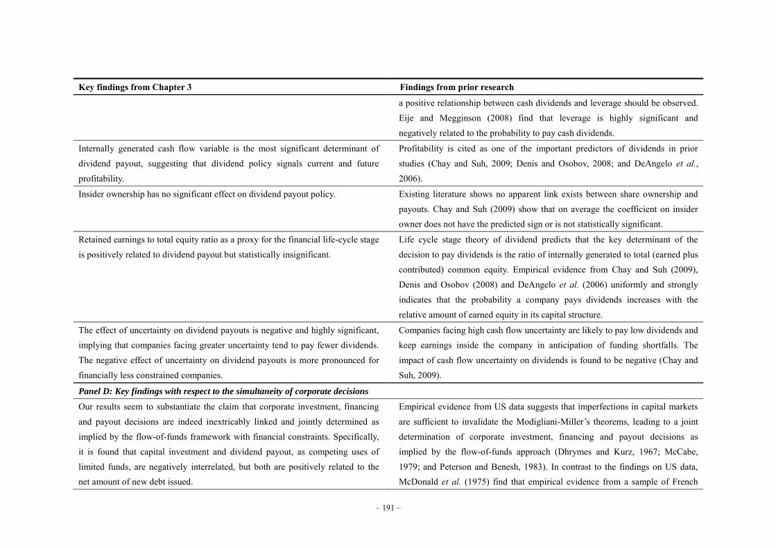
– 191 –
Key findings from Chapter 3 Findings from prior research
a positive relationship between cash dividends and leverage should be observed. Eije and Megginson (2008) find that leverage is highly significant and negatively related to the probability to pay cash dividends.
Internally generated cash flow variable is the most significant determinant of dividend payout, suggesting that dividend policy signals current and future profitability.
Profitability is cited as one of the important predictors of dividends in prior studies (Chay and Suh, 2009; Denis and Osobov, 2008; and DeAngelo et al., 2006).
Insider ownership has no significant effect on dividend payout policy. Existing literature shows no apparent link exists between share ownership and payouts. Chay and Suh (2009) show that on average the coefficient on insider owner does not have the predicted sign or is not statistically significant.
Retained earnings to total equity ratio as a proxy for the financial life-cycle stage is positively related to dividend payout but statistically insignificant.
Life cycle stage theory of dividend predicts that the key determinant of the decision to pay dividends is the ratio of internally generated to total (earned plus contributed) common equity. Empirical evidence from Chay and Suh (2009), Denis and Osobov (2008) and DeAngelo et al. (2006) uniformly and strongly indicates that the probability a company pays dividends increases with the relative amount of earned equity in its capital structure.
The effect of uncertainty on dividend payouts is negative and highly significant, implying that companies facing greater uncertainty tend to pay fewer dividends. The negative effect of uncertainty on dividend payouts is more pronounced for financially less constrained companies.
Companies facing high cash flow uncertainty are likely to pay low dividends and keep earnings inside the company in anticipation of funding shortfalls. The impact of cash flow uncertainty on dividends is found to be negative (Chay and Suh, 2009).
Panel D: Key findings with respect to the simultaneity of corporate decisions
Our results seem to substantiate the claim that corporate investment, financing and payout decisions are indeed inextricably linked and jointly determined as implied by the flow-of-funds framework with financial constraints. Specifically, it is found that capital investment and dividend payout, as competing uses of limited funds, are negatively interrelated, but both are positively related to the net amount of new debt issued.
Empirical evidence from US data suggests that imperfections in capital markets are sufficient to invalidate the Modigliani-Miller’s theorems, leading to a joint determination of corporate investment, financing and payout decisions as implied by the flow-of-funds approach (Dhrymes and Kurz, 1967; McCabe, 1979; and Peterson and Benesh, 1983). In contrast to the findings on US data, McDonald et al. (1975) find that empirical evidence from a sample of French
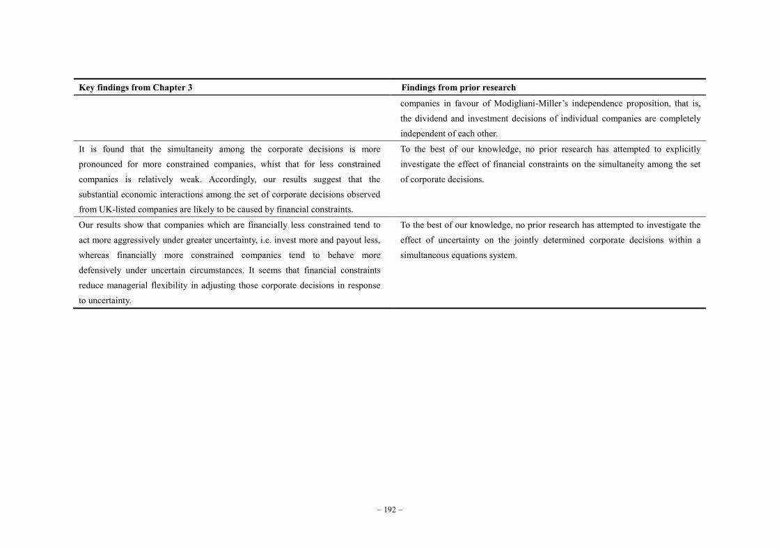
– 192 –
Key findings from Chapter 3 Findings from prior research
companies in favour of Modigliani-Miller’s independence proposition, that is, the dividend and investment decisions of individual companies are completely independent of each other.
It is found that the simultaneity among the corporate decisions is more pronounced for more constrained companies, whist that for less constrained companies is relatively weak. Accordingly, our results suggest that the substantial economic interactions among the set of corporate decisions observed from UK-listed companies are likely to be caused by financial constraints.
To the best of our knowledge, no prior research has attempted to explicitly investigate the effect of financial constraints on the simultaneity among the set of corporate decisions.
Our results show that companies which are financially less constrained tend to act more aggressively under greater uncertainty, i.e. invest more and payout less, whereas financially more constrained companies tend to behave more defensively under uncertain circumstances. It seems that financial constraints reduce managerial flexibility in adjusting those corporate decisions in response to uncertainty.
To the best of our knowledge, no prior research has attempted to investigate the effect of uncertainty on the jointly determined corporate decisions within a simultaneous equations system.
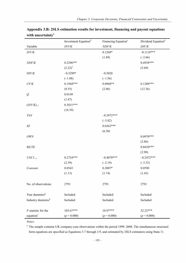
Chapter 3: Corporate Decisions, Financial Constraints and Uncertainty
– 193 –
Appendix 3.B: 2SLS estimation results for investment, financing and payout equations with uncertaintya Variable
Investment Equationb INV/K
Financing Equationc NDF/K
Dividend Equationd DIV/K
INV/K 0.1268* (1.89)
–0.1118*** (–2.66)
NDF/K 0.2296**e (2.22)f
0.4938*** (5.69)
DIV/K –0.3299* (–1.88)
–0.5028 (–1.56)
CF/K 0.1944*** (8.55)
0.0968** (2.06)
0.1288*** (12.36)
Q 0.0149 (1.47)
(INV/K)–1 0.3031*** (18.39)
TAN –0.3972*** (–3.82)
SZ 0.0363*** (6.30)
OWN 0.0970*** (2.86)
RE/TE 0.0410*** (2.90)
UNC1–1 0.2724*** (2.59)
–0.4070*** (–2.19)
–0.2472*** (–3.33)
Constant 0.0543 (1.13)
0.2007* (1.74)
0.0590 (1.43)
No. of observations
2791 2791 2791
Year dummiesg Included Included Included
Industry dummiesh
Included Included Included
F-statistic for the equationi
105.67*** (p = 0.000)
10.97*** (p = 0.000)
52.22*** (p = 0.000)
Notes: a. The sample contains UK company-year observations within the period 1999–2008. The simultaneous structural
form equations are specified as Equations 3.7 through 3.9, and estimated by 2SLS estimators using Stata 11.

Chapter 3: Corporate Decisions, Financial Constraints and Uncertainty
– 194 –
b. Investment equation is specified as 161543210 1///// UNCKINVQKCFKDIVKNDFKINV .
c. Financing equation is specified as 16543210 1//// UNCSZTANKCFKDIVKINVKNDF .
d. Dividend equation is specified as 16543210 1///// UNCTEREOWNKCFKNDFKINVKDIV .
e. * significant at the 10% level; ** significant at the 5% level; and *** significant at the 1% level. f. t-statistics are reported in parentheses. g. Year dummies are included in all of the equations to account for the time effect. h. Industry dummies are included in all of the equations to account for the inter-industry variations. i. F-statistic tests the null hypothesis that all of the coefficients except the intercept coefficient are jointly zero.
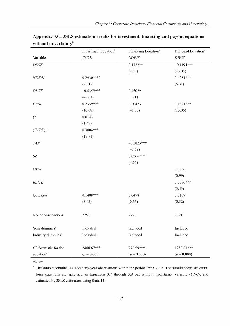
Chapter 3: Corporate Decisions, Financial Constraints and Uncertainty
– 195 –
Appendix 3.C: 3SLS estimation results for investment, financing and payout equations without uncertaintya Variable
Investment Equationb INV/K
Financing Equationc NDF/K
Dividend Equationd DIV/K
INV/K 0.1722** (2.53)
–0.1194*** (–3.05)
NDF/K 0.2930***e (2.81)f
0.4281*** (5.31)
DIV/K –0.6359*** (–3.61)
0.4502* (1.71)
CF/K 0.2359*** (10.68)
–0.0423 (–1.05)
0.1321*** (13.06)
Q 0.0143 (1.47)
(INV/K)–1 0.3004*** (17.81)
TAN –0.2823*** (–3.39)
SZ 0.0266*** (4.64)
OWN 0.0256 (0.99)
RE/TE 0.0376*** (3.43)
Constant 0.1488*** (3.45)
0.0478 (0.66)
0.0107 (0.32)
No. of observations
2791 2791 2791
Year dummiesg Included Included Included
Industry dummiesh
Included Included Included
Chi2-statistic for the equationi
2488.67*** (p = 0.000)
276.59*** (p = 0.000)
1259.81*** (p = 0.000)
Notes: a. The sample contains UK company-year observations within the period 1999–2008. The simultaneous structural
form equations are specified as Equations 3.7 through 3.9 but without uncertainty variable (UNC), and estimated by 3SLS estimators using Stata 11.

Chapter 3: Corporate Decisions, Financial Constraints and Uncertainty
– 196 –
b. Investment equation is specified as 1543210 ///// KINVQKCFKDIVKNDFKINV .
c. Financing equation is specified as SZTANKCFKDIVKINVKNDF 543210 //// .
d. Dividend equation is specified as TEREOWNKCFKNDFKINVKDIV ///// 543210 .
e. * significant at the 10% level; ** significant at the 5% level; and *** significant at the 1% level. f. z-statistics are reported in parentheses. g. Year dummies are included in all of the equations to account for the time effect. h. Industry dummies are included in all of the equations to account for the inter-industry variations. i. Chi2-statistic tests the null hypothesis that all of the coefficients except the intercept coefficient are jointly zero.
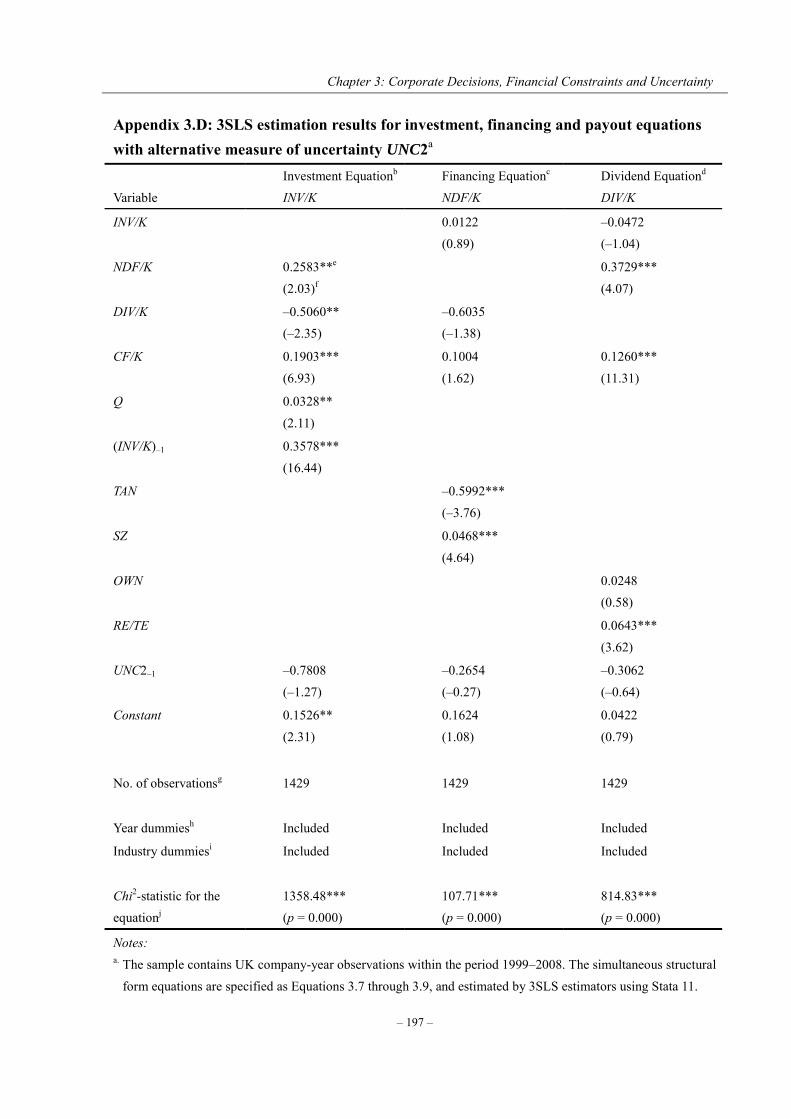
Chapter 3: Corporate Decisions, Financial Constraints and Uncertainty
– 197 –
Appendix 3.D: 3SLS estimation results for investment, financing and payout equations with alternative measure of uncertainty UNC2a Variable
Investment Equationb INV/K
Financing Equationc NDF/K
Dividend Equationd DIV/K
INV/K 0.0122 (0.89)
–0.0472 (–1.04)
NDF/K 0.2583**e (2.03)f
0.3729*** (4.07)
DIV/K –0.5060** (–2.35)
–0.6035 (–1.38)
CF/K 0.1903*** (6.93)
0.1004 (1.62)
0.1260*** (11.31)
Q 0.0328** (2.11)
(INV/K)–1 0.3578*** (16.44)
TAN –0.5992*** (–3.76)
SZ 0.0468*** (4.64)
OWN 0.0248 (0.58)
RE/TE 0.0643*** (3.62)
UNC2–1 –0.7808 (–1.27)
–0.2654 (–0.27)
–0.3062 (–0.64)
Constant 0.1526** (2.31)
0.1624 (1.08)
0.0422 (0.79)
No. of observationsg
1429 1429 1429
Year dummiesh Included Included Included
Industry dummiesi
Included Included Included
Chi2-statistic for the equationj
1358.48*** (p = 0.000)
107.71*** (p = 0.000)
814.83*** (p = 0.000)
Notes: a. The sample contains UK company-year observations within the period 1999–2008. The simultaneous structural
form equations are specified as Equations 3.7 through 3.9, and estimated by 3SLS estimators using Stata 11.

Chapter 3: Corporate Decisions, Financial Constraints and Uncertainty
– 198 –
b. Investment equation is specified as 161543210 2///// UNCKINVQKCFKDIVKNDFKINV .
c. Financing equation is specified as 16543210 2//// UNCSZTANKCFKDIVKINVKNDF .
d. Dividend equation is specified as 16543210 2///// UNCTEREOWNKCFKNDFKINVKDIV .
e. * significant at the 10% level; ** significant at the 5% level; and *** significant at the 1% level. f. z-statistics are reported in parentheses. g. The number of observation reduced to 1,429 because the accounting items used to compute corporate decision
variables and company characteristic variables are collected from the Worldscope database, whereas the daily stock returns used to derive UNC2 are collected from the DataStream database. The merge of datasets results in significant decrease in the number of observations.
h. Year dummies are included in all of the equations to account for the time effect. i. Industry dummies are included in all of the equations to account for the inter-industry variations. j. Chi2-statistic tests the null hypothesis that all of the coefficients except the intercept coefficient are jointly zero.
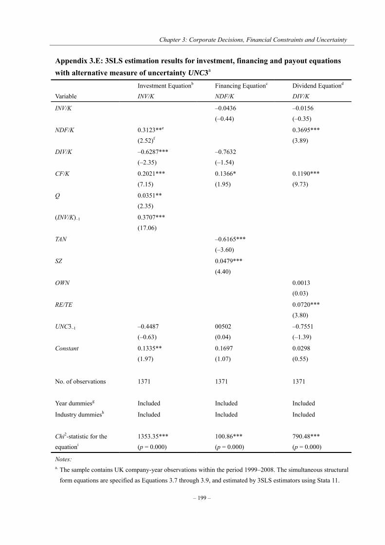
Chapter 3: Corporate Decisions, Financial Constraints and Uncertainty
– 199 –
Appendix 3.E: 3SLS estimation results for investment, financing and payout equations with alternative measure of uncertainty UNC3a Variable
Investment Equationb INV/K
Financing Equationc NDF/K
Dividend Equationd DIV/K
INV/K –0.0436 (–0.44)
–0.0156 (–0.35)
NDF/K 0.3123**e (2.52)f
0.3695*** (3.89)
DIV/K –0.6287*** (–2.35)
–0.7632 (–1.54)
CF/K 0.2021*** (7.15)
0.1366* (1.95)
0.1190*** (9.73)
Q 0.0351** (2.35)
(INV/K)–1 0.3707*** (17.06)
TAN –0.6165*** (–3.60)
SZ 0.0479*** (4.40)
OWN 0.0013 (0.03)
RE/TE 0.0720*** (3.80)
UNC3–1 –0.4487 (–0.63)
00502 (0.04)
–0.7551 (–1.39)
Constant 0.1335** (1.97)
0.1697 (1.07)
0.0298 (0.55)
No. of observations
1371 1371 1371
Year dummiesg Included Included Included
Industry dummiesh
Included Included Included
Chi2-statistic for the equationi
1353.35*** (p = 0.000)
100.86*** (p = 0.000)
790.48*** (p = 0.000)
Notes: a. The sample contains UK company-year observations within the period 1999–2008. The simultaneous structural
form equations are specified as Equations 3.7 through 3.9, and estimated by 3SLS estimators using Stata 11.

Chapter 3: Corporate Decisions, Financial Constraints and Uncertainty
– 200 –
b. Investment equation is specified as 161543210 3///// UNCKINVQKCFKDIVKNDFKINV .
c. Financing equation is specified as 16543210 3//// UNCSZTANKCFKDIVKINVKNDF .
d. Dividend equation is specified as 16543210 3///// UNCTEREOWNKCFKNDFKINVKDIV .
e. * significant at the 10% level; ** significant at the 5% level; and *** significant at the 1% level. f. z-statistics are reported in parentheses. g. The number of observation reduced to 1,371 because the accounting items used to compute corporate decision
variables and company characteristic variables are collected from the Worldscope database, whereas the daily stock returns used to derive UNC3 are collected from the DataStream database. The merge of datasets results in significant decrease in the number of observations. The number of observations further reduces by excluding companies whose stock returns do not exhibit GARCH effect and thus UNC3 cannot be derived,
h. Year dummies are included in all of the equations to account for the time effect. i. Industry dummies are included in all of the equations to account for the inter-industry variations. j. Chi2-statistic tests the null hypothesis that all of the coefficients except the intercept coefficient are jointly zero.
Chapter 4: Corporate Decisions, Managerial Confidence and Economic Sentiment
– 201 –
CHAPTER 4
CORPORATE DECISIONS, MANAGERIAL CONFIDENCE
AND ECONOMIC SENTIMENT
4.1 Introduction
Managerial confidence and economic sentiment are frequently cited and closely followed by
practitioners, government bodies, financial institutions, research institutes and news media for
both qualitative and quantitative analysis purposes. In his General Theory, Keynes (1936)
links the notion of “sentiment” to the “state of long-term expectation” and the “state of
confidence”. The level of confidence or sentiment reflects the prevailing attitude of economic
agents towards anticipated economic and business developments. It is believed that they play
key roles in the formation of companies’ expectations of future profit levels, and hence in the
determination of their key corporate decisions. A high level of managerial confidence or
economic sentiment creates favourable environment for a business to grow; conversely, a low
confidence or sentiment level indicates a negative outlook for future business spending and
capital investment. However, the concepts of managerial confidence and economic sentiment
have not been embraced entirely into mainstream financial economics, which relies heavily on
the rigid assumption of broad rationality in corporate decision-making processes. As
researchers add more and more company fundamental characteristics in explaining corporate
behaviour, these hard-to-define ideas such as managerial confidence and economic sentiment

Chapter 4: Corporate Decisions, Managerial Confidence and Economic Sentiment
– 202 –
are largely ignored and excluded from their empirical models. It is noted that the major
challenge for incorporating such ideas into economic models is to construct plausible proxies
for the state of confidence and sentiment (see Malmendier and Tate, 2005).
This chapter represents one of the first studies to explicitly and systematically
incorporate the state of managerial confidence and economic sentiment into the area of
corporate finance. We employ a number of direct measures of agents’ perceptions about
current and expected business and economic conditions to explore their potential effects on
corporate investment, financing and payout decisions. These direct measures of the state of
economic sentiment and managerial confidence are drawn up from a series of qualitative
economic surveys of managers in four main industry sectors as well as consumers across the
European Union (EU) member states and candidate countries. The surveys are carried out by
the Directorate-General for Economic and Financial Affairs (DG-ECFIN) of the European
Commission (described in detail in Section 4.2). These novel measures of the state of
confidence and sentiment are forward-looking in nature, and therefore are completely
different from the ex post variables typically used in the previous literature.34 The managerial
confidence and economic sentiment indicators employed in this chapter are expected to
represent managers’ collective attitude towards the future prospects of the companies, the
sectors and the economies at aggregate levels.
34 Previous studies typically assume rational expectations by using ex post variables such as GDP, industrial production or aggregate consumption as proxies for economic sentiment. The use of director measures of economic sentiment and managerial confidence obtained from the survey of agents’ expectations about economic and business conditions should, to a considerable degree, eliminate noise that may exist in ex post variables.
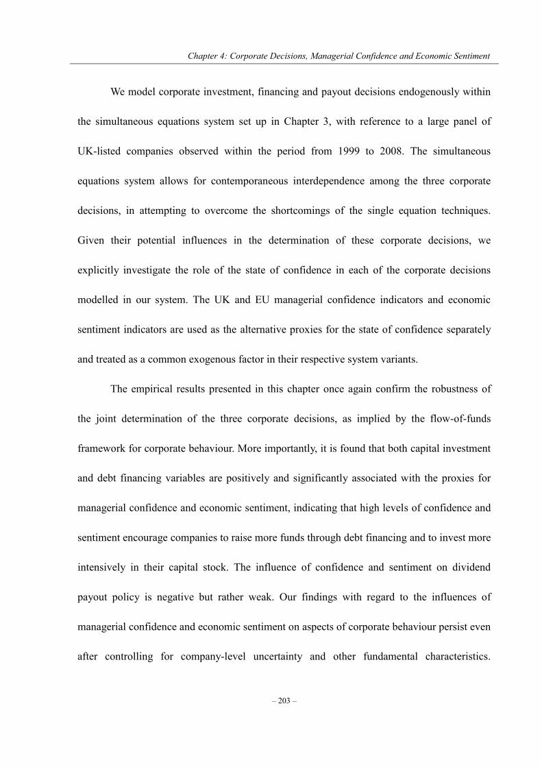
Chapter 4: Corporate Decisions, Managerial Confidence and Economic Sentiment
– 203 –
We model corporate investment, financing and payout decisions endogenously within
the simultaneous equations system set up in Chapter 3, with reference to a large panel of
UK-listed companies observed within the period from 1999 to 2008. The simultaneous
equations system allows for contemporaneous interdependence among the three corporate
decisions, in attempting to overcome the shortcomings of the single equation techniques.
Given their potential influences in the determination of these corporate decisions, we
explicitly investigate the role of the state of confidence in each of the corporate decisions
modelled in our system. The UK and EU managerial confidence indicators and economic
sentiment indicators are used as the alternative proxies for the state of confidence separately
and treated as a common exogenous factor in their respective system variants.
The empirical results presented in this chapter once again confirm the robustness of
the joint determination of the three corporate decisions, as implied by the flow-of-funds
framework for corporate behaviour. More importantly, it is found that both capital investment
and debt financing variables are positively and significantly associated with the proxies for
managerial confidence and economic sentiment, indicating that high levels of confidence and
sentiment encourage companies to raise more funds through debt financing and to invest more
intensively in their capital stock. The influence of confidence and sentiment on dividend
payout policy is negative but rather weak. Our findings with regard to the influences of
managerial confidence and economic sentiment on aspects of corporate behaviour persist even
after controlling for company-level uncertainty and other fundamental characteristics.
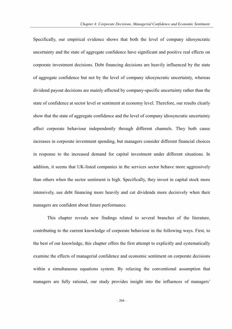
Chapter 4: Corporate Decisions, Managerial Confidence and Economic Sentiment
– 204 –
Specifically, our empirical evidence shows that both the level of company idiosyncratic
uncertainty and the state of aggregate confidence have significant and positive real effects on
corporate investment decisions. Debt financing decisions are heavily influenced by the state
of aggregate confidence but not by the level of company idiosyncratic uncertainty, whereas
dividend payout decisions are mainly affected by company-specific uncertainty rather than the
state of confidence at sector level or sentiment at economy level. Therefore, our results clearly
show that the state of aggregate confidence and the level of company idiosyncratic uncertainty
affect corporate behaviour independently through different channels. They both cause
increases in corporate investment spending, but managers consider different financial choices
in response to the increased demand for capital investment under different situations. In
addition, it seems that UK-listed companies in the services sector behave more aggressively
than others when the sector sentiment is high. Specifically, they invest in capital stock more
intensively, use debt financing more heavily and cut dividends more decisively when their
managers are confident about future performance.
This chapter reveals new findings related to several branches of the literature,
contributing to the current knowledge of corporate behaviour in the following ways. First, to
the best of our knowledge, this chapter offers the first attempt to explicitly and systematically
examine the effects of managerial confidence and economic sentiment on corporate decisions
within a simultaneous equations system. By relaxing the conventional assumption that
managers are fully rational, our study provides insight into the influences of managers’

Chapter 4: Corporate Decisions, Managerial Confidence and Economic Sentiment
– 205 –
psychological bias on aspects of corporate behaviour, adding to the small but growing
literature on behavioural corporate finance. Second, our study highlights and discriminates the
roles played by the degree of uncertainty and by the state of confidence, in the determination
of corporate decisions. Our findings contribute to the literature by providing empirical
evidence that they both influence corporate policies but independently through different
mechanisms. Besides, we carry out a comparison across four main industry sectors, revealing
additional insights into the influences of managerial confidence and economic sentiment on
the behaviour of companies with different characteristics.
The remainder of this chapter is organised as follows. Section 4.2 describes the novel
measures of sector-specific managerial confidence and economic sentiment used in this
chapter. Section 4.3 specifies the empirical models. Section 4.4 discusses the sample,
variables and preliminary analysis. Section 4.5 describes the estimation and testing procedures
as well as the main results for the empirical models. Section 4.6 offers further evidence to
check the robustness of our findings. Concluding remarks are drawn in Section 4.7.
4.2 Measures of managerial confidence and economic sentiment
The biggest challenge in incorporating the concepts of managerial confidence and economic
sentiment into corporate behavioural modelling is to construct plausible measures of these
hard-to-define ideas (see Malmendier and Tate, 2005). Previous studies under the assumption
of rational expectations typically employ ex post variables such as gross domestic product
(GDP), industrial production or aggregate consumption as proxies for economic sentiment.

Chapter 4: Corporate Decisions, Managerial Confidence and Economic Sentiment
– 206 –
Recent literature in behavioural corporate finance proposes more creative methods to proxy
for managerial confidence. For example, Malmendier et al. (2011) and Malmendier and Tate
(2005) exploit the overexposure of CEOs to the idiosyncratic risk of their companies, as
reflected by their personal portfolio of their companies’ options and stockholdings, to measure
managerial confidence in the US. Ben-David et al. (2007) measure overconfidence based on
CFOs’ confidence intervals of their stock market predictions. Lin et al. (2005) construct a
managerial confidence measure for Taiwanese companies based on CEOs’ forecast errors in
their companies’ future earnings. Unfortunately, such data used to construct measures of
managerial confidence at individual manager level are not publicly available in the UK.
Unlike prior studies, the confidence indicators employed in the present study are direct
measures of managerial confidence and economic sentiment drawn from the Joint
Harmonised EU Programme of Business and Consumer Surveys. The surveys are carried out
by the European Commission Directorate-General for Economic and Financial Affairs
(DG-ECFIN) across EU member states and candidate countries, aiming to obtain insights into
the beliefs of economic agents, providing essential information for economic surveillance,
short-term forecasting and economic research. Their results are often considered as early
indicators for future economic developments (European Commission, 2007). The results of all
surveys and the readings of all indicators are publicly available from the European
Commission website. 35 The sample sizes for the Joint Harmonised EU Business and
35 See the European Commission website via http://ec.europa.eu.

Chapter 4: Corporate Decisions, Managerial Confidence and Economic Sentiment
– 207 –
Consumer Surveys across countries can be found in Appendix 4.A. According to European
Commission (2007), approximately 124,000 companies and almost 40,000 consumers are
currently surveyed each month across the European Union, among which 3,800 companies
and 2,000 consumers are surveyed in the UK. This chapter, therefore, focuses on managerial
confidence and economic sentiment in the UK as well as their counterparts at EU level, using
monthly data for the period from January 1999 to December 2008.
4.2.1 Sector-specific managerial confidence indicators
The general business and consumer surveys dataset is composed of five sets of sector-specific
survey data, namely, industry (INDU), services (SERV), consumer (CONS), retail trade (RETA)
and construction (BUIL).36 For each sector, several questions are asked in each survey (see
Appendix 4.B for the complete questionnaires). Nearly all of the survey questions are of a
qualitative nature, trying to assess the recent trends in business situations and monitor the
current status of the economy. Typically, the survey questions have similar answer schemes
which are given according to a three- or five-option ordinal scale, from optimism to
pessimism. More specifically, the three-option questions have alternative answers of
“positive”, “neutral” and “negative”. The questionnaires are addressed to senior managers,
such as Chairmen, CEOs or functional directors, of the sample companies in each of the
sectors, as well as to consumers. Answers obtained from the surveys are aggregated and
36 To be precise, industry (INDU) refers to manufacturing industry in the Joint Harmonised EU Programme of Business and Consumer Surveys (European Commission, 2007).

Chapter 4: Corporate Decisions, Managerial Confidence and Economic Sentiment
– 208 –
expressed in the form of a “balance” for each equation which is defined as the difference
between the percentages of respondents giving positive and negative replies,
MPB (4.1)
where P denotes the percentage of positive replies, E denotes the percentage of neutral replies,
M denotes the percentage of negative replies, and therefore %100 MEP . B denotes
aggregate balance which is the percentage of net positive or optimistic responses. In the case
of questions with five options, i.e. “very positive” and “very negative” in addition to the three
options mentioned above, the balances are defined as the weighted average of the responses as
follows,
)21()
21( MMMPPPB (4.2)
where PP denotes the percentage of very positive replies, MM denotes the percentage of very
negative replies, and hence %100 MMMEPPP . According to above definitions,
the balance values have a possible range between -100% and 100%. The balance value equals
100% (-100%) if all respondents choose the positive (negative) option in the case of
three-option questions, or the most positive (negative) option in the case of five-option
questions.

Chapter 4: Corporate Decisions, Managerial Confidence and Economic Sentiment
– 209 –
Based on the responses to a selection of survey questions, which are closely related to
the reference variables they are supposed to track (e.g. industrial production), the
sector-specific confidence indicators (SCI) are constructed for each of the five sectors. The
questions selected to construct the confidence indicator for each sector mainly focus on the
development of the business situation over the past few months, the current situation of the
business, and the expectation of changes in business activities over the next few months. The
sector-specific confidence indicators are defined as the arithmetic average of the balances (in
percentage points) of the answers to the selected questions,37
n
BSCI
n
ii
1 (4.3)
where SCI stands for a sector-specific confidence indicator, Bi denotes the balance of the
answers to question i in the corresponding sector-specific survey, and n is the number of
questions selected to build the confidence indicator. It is worth noting that the balances of the
answers to some of the selected questions enter Equation 4.3 with inverted signs (see the
notes attached to Appendix 4.B). The sector-specific confidence indicators for the industry,
services, retail trade and construction sectors thus reflect the collective perceptions and
confidence of the managers towards future business development at sector level. For each of
37 The balance series from the selected questions are not standardised prior to their aggregation. The balance series used to calculate each confidence indicator are seasonally adjusted (European Commission, 2007).
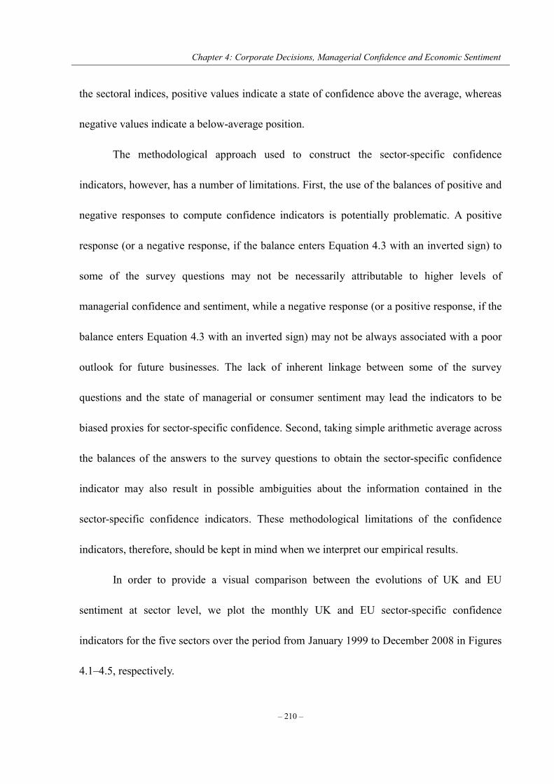
Chapter 4: Corporate Decisions, Managerial Confidence and Economic Sentiment
– 210 –
the sectoral indices, positive values indicate a state of confidence above the average, whereas
negative values indicate a below-average position.
The methodological approach used to construct the sector-specific confidence
indicators, however, has a number of limitations. First, the use of the balances of positive and
negative responses to compute confidence indicators is potentially problematic. A positive
response (or a negative response, if the balance enters Equation 4.3 with an inverted sign) to
some of the survey questions may not be necessarily attributable to higher levels of
managerial confidence and sentiment, while a negative response (or a positive response, if the
balance enters Equation 4.3 with an inverted sign) may not be always associated with a poor
outlook for future businesses. The lack of inherent linkage between some of the survey
questions and the state of managerial or consumer sentiment may lead the indicators to be
biased proxies for sector-specific confidence. Second, taking simple arithmetic average across
the balances of the answers to the survey questions to obtain the sector-specific confidence
indicator may also result in possible ambiguities about the information contained in the
sector-specific confidence indicators. These methodological limitations of the confidence
indicators, therefore, should be kept in mind when we interpret our empirical results.
In order to provide a visual comparison between the evolutions of UK and EU
sentiment at sector level, we plot the monthly UK and EU sector-specific confidence
indicators for the five sectors over the period from January 1999 to December 2008 in Figures
4.1–4.5, respectively.
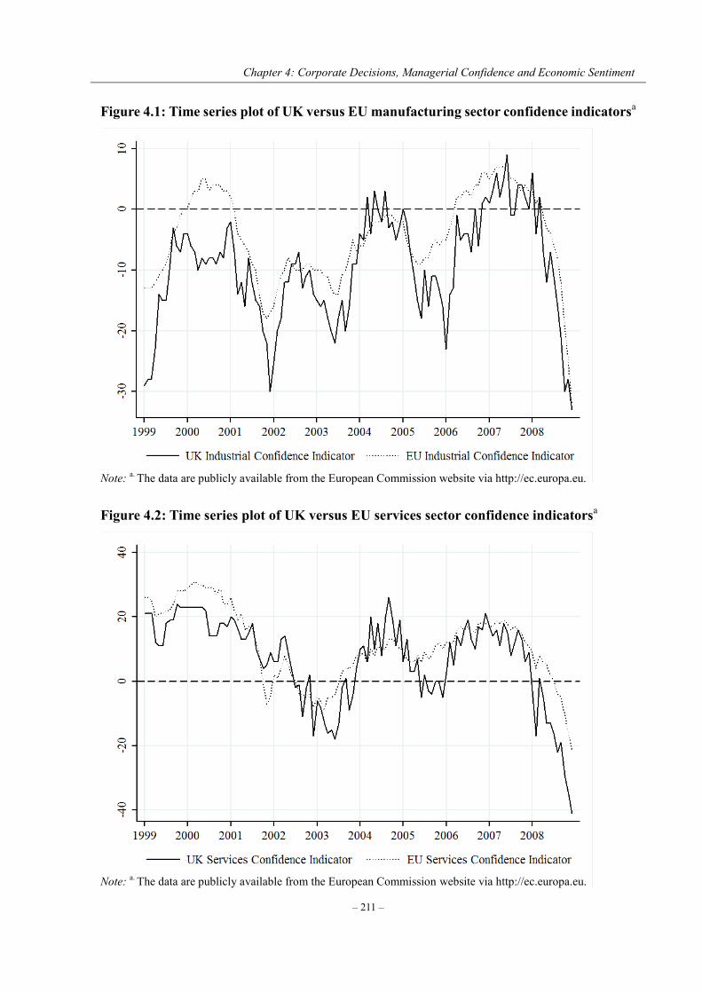
Chapter 4: Corporate Decisions, Managerial Confidence and Economic Sentiment
– 211 –
Figure 4.1: Time series plot of UK versus EU manufacturing sector confidence indicatorsa
Figure 4.2: Time series plot of UK versus EU services sector confidence indicatorsa
Note: a. The data are publicly available from the European Commission website via http://ec.europa.eu.
Note: a. The data are publicly available from the European Commission website via http://ec.europa.eu.
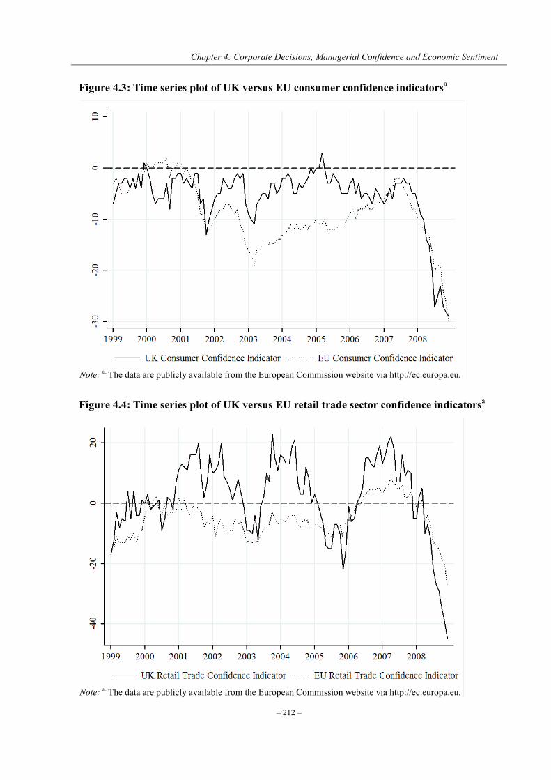
Chapter 4: Corporate Decisions, Managerial Confidence and Economic Sentiment
– 212 –
Figure 4.3: Time series plot of UK versus EU consumer confidence indicatorsa
Figure 4.4: Time series plot of UK versus EU retail trade sector confidence indicatorsa
Note: a. The data are publicly available from the European Commission website via http://ec.europa.eu.
Note: a. The data are publicly available from the European Commission website via http://ec.europa.eu.
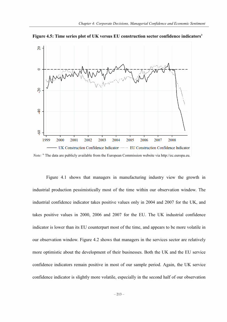
Chapter 4: Corporate Decisions, Managerial Confidence and Economic Sentiment
– 213 –
Figure 4.5: Time series plot of UK versus EU construction sector confidence indicatorsa
Figure 4.1 shows that managers in manufacturing industry view the growth in
industrial production pessimistically most of the time within our observation window. The
industrial confidence indicator takes positive values only in 2004 and 2007 for the UK, and
takes positive values in 2000, 2006 and 2007 for the EU. The UK industrial confidence
indicator is lower than its EU counterpart most of the time, and appears to be more volatile in
our observation window. Figure 4.2 shows that managers in the services sector are relatively
more optimistic about the development of their businesses. Both the UK and the EU service
confidence indicators remain positive in most of our sample period. Again, the UK service
confidence indicator is slightly more volatile, especially in the second half of our observation
Note: a. The data are publicly available from the European Commission website via http://ec.europa.eu.

Chapter 4: Corporate Decisions, Managerial Confidence and Economic Sentiment
– 214 –
window. Consumers seem to be rather pessimistic about the financial conditions of their
households as well as the economic situation in general, as shown in Figure 4.3. Compared
with consumers in the EU as a whole, UK consumers are less pessimistic most of the time
from 2002 to 2007. Figure 4.4 plots UK and EU retail trade sector confidence indicators over
time. Managerial confidence in the retail trade sector in the UK outperforms that in the EU.
However, the UK retail trade sector confidence indicator displays a rather large fluctuation,
while the EU indicator is relatively stable over time. Figure 4.5 shows that the construction
sector confidence indicators for the UK and the EU are less correlated with each other, other
than being rather stable before 2008. There is no systematic pattern of one being consistently
higher than the other. In all figures we can notice the magnitude of the downward shift in
managerial confidence that characterises the last two years of the time series. The causes of
the downwards shift may largely be attributed to the global financial crisis starts in late 2007.
4.2.2 Economic sentiment indicators
Based on the complete set of 15 balance series underlying the five sector-specific confidence
indicators, the economic sentiment indicator (ESI) is formulated to synthesise the information
contained in the individual surveys into a single variable, in an attempt to track the economy
as a whole. Thus, this composite indicator can be considered as an aggregate indicator which
summarises the information contained in the five sector-specific confidence indicators
(European Commission, 2007). The economic sentiment indicator is defined as the weighted
average of the standardised balance series, in which explicit weights are allocated to the five

Chapter 4: Corporate Decisions, Managerial Confidence and Economic Sentiment
– 215 –
surveyed sectors, i.e. industry 40%, services 30%, consumers 20%, retail trade 5% and
construction 5%.38
More specifically, the steps of the calculation of the economic sentiment indicator,
according to European Commission (2007), can be summarised as follows. First, the balance
series underlying the sector-specific confidence indicators are standardised,
j
jtjt S
BBY
(4.4)
where Bjt is the seasonally adjusted balance series j underlying the confidence indicators at
time t, jB is the arithmetic average of the balance series j, i.e. TBB T
t jtj /11
, and jS
is the sample standard deviation of the balance series j, i.e. )1/()(1
2 TBBS T
t jjtj .39
Hence, jtY is the standardised balance series j. The available standardised balance series are
then used to compute the weighted average Zt as follows,
tj
j
jjtj
t w
YwZ
)(
(4.5)
38 The given weights are determined according to two criteria, namely, “representativeness” of the sector in question and tracking performance in relation to the reference variable. Corresponding to the broad scope of the Economic Sentiment Indicator, the obvious reference variable is GDP growth, tracking the movements of the economy as a whole. It is important to note that the weights are not directly applied to the five confidence indicators themselves but to their standardised individual component series (European Commission, 2007). 39 The moments for standardisation are computed over a frozen sample to avoid monthly revisions of the index. Currently, the sample runs from January 1990 to December 2006, i.e. T = 204 (European Commission, 2007).

Chapter 4: Corporate Decisions, Managerial Confidence and Economic Sentiment
– 216 –
where wj is the weight of standardised balance series j used to construct the economic
sentiment indicator, which is computed as the sector weights mentioned above divided by the
number of balance series making up the related sector-specific confidence indicator.40
tj jw )( is the sum of the weights of the available series at time t. Thus, Zt can be viewed as
the weighted average of standardised balance series, if all 15 components are available;
otherwise, it is the weighted sum of the available balance series divided by the sum of the
allocated weights of the available components. Then, the weighted average Zt is standardised
and scaled as follows,
10010)(
Z
t
SZZESI (4.6)
where Z and ZS are the arithmetic average and the standard deviation of Z, which are
computed as TZZ T
t t /1
and )1/()(
12
TZZS T
t tZ . The standardised Zt is
scaled to have a long-term mean of 100% and a standard deviation of 10%.41 Finally, the
aggregate ESI for the EU is calculated as a weighted average of the ESI of each member state.
The weights utilised to calculate the ESI for the EU take into account the relative volume of
each economy within the European Union, and are revised periodically.
40 For example, there are three balance series related to the service confidence indicator, thus each of the standardised balances receive a weight of 10%, adding up to the total services sector weight of 30%. 41 According to European Commission (2007), the imposed standard deviation of 10 implies that in about 68% of the cases the economic sentiment indicator will be within the range of 90 to 110, assuming the indicator is normally distributed.
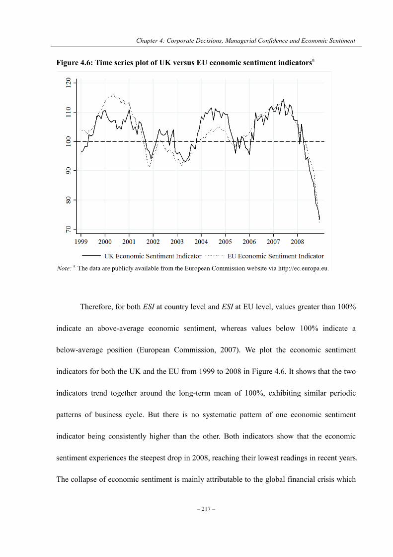
Chapter 4: Corporate Decisions, Managerial Confidence and Economic Sentiment
– 217 –
Figure 4.6: Time series plot of UK versus EU economic sentiment indicatorsa
Therefore, for both ESI at country level and ESI at EU level, values greater than 100%
indicate an above-average economic sentiment, whereas values below 100% indicate a
below-average position (European Commission, 2007). We plot the economic sentiment
indicators for both the UK and the EU from 1999 to 2008 in Figure 4.6. It shows that the two
indicators trend together around the long-term mean of 100%, exhibiting similar periodic
patterns of business cycle. But there is no systematic pattern of one economic sentiment
indicator being consistently higher than the other. Both indicators show that the economic
sentiment experiences the steepest drop in 2008, reaching their lowest readings in recent years.
The collapse of economic sentiment is mainly attributable to the global financial crisis which
Note: a. The data are publicly available from the European Commission website via http://ec.europa.eu.

Chapter 4: Corporate Decisions, Managerial Confidence and Economic Sentiment
– 218 –
starts in late 2007 and deteriorates in 2008.
Although the sector-specific managerial confidence indicators and the economic
sentiment indicators are published at a monthly frequency, corporate decision variables and
company characteristics variables are only available at an annual frequency. To empirically
investigate the influence of managerial confidence and economic sentiment on corporate
decisions, we have to convert the monthly-frequency indicators into their annual-frequency
analogues. We therefore calculate the arithmetic averages of the monthly values over each
calendar year as our proxies for managerial confidence and economic sentiment for the
corresponding period. Given the argument that the key corporate decisions are likely to be
made at the beginning of each fiscal year, the state of managerial confidence and economic
sentiment in December tends to play a more important role than that in the other months of a
year in making corporate decisions for the year ahead (Oliver and Mefteh, 2010). Therefore,
we also consider the December figures as the relevant measures of managerial confidence and
economic sentiment to check the robustness of our empirical results obtained using the
arithmetic averages.42
Table 4.1 presents the descriptive statistics of the UK and the EU indicators at both
monthly frequency and annual frequency observed over the period from January 1999 to
December 2008
42 Oliver and Mefteh (2010) take the December figure as the relevant measure of manager confidence to investigate the effect of confidence on the capital structure choices of a panel of French companies.
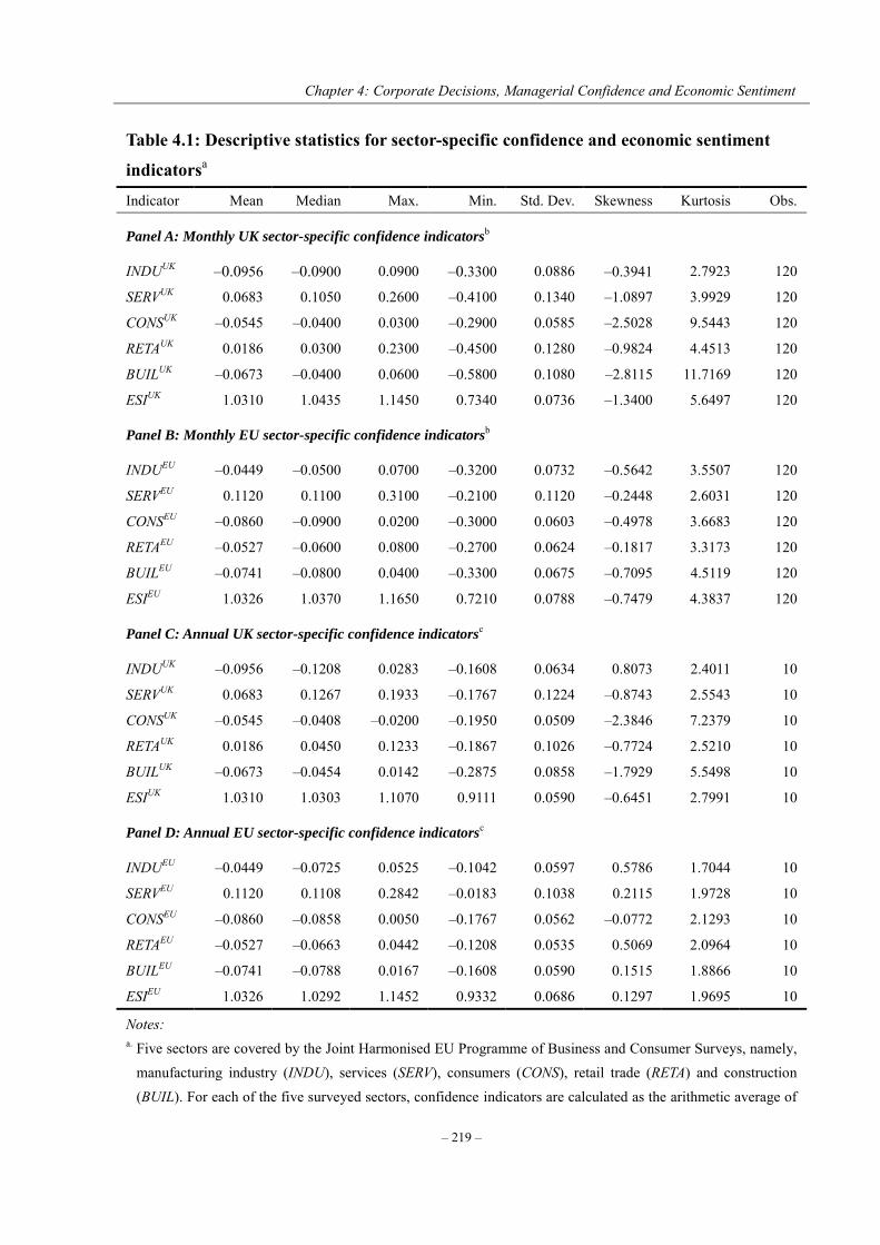
Chapter 4: Corporate Decisions, Managerial Confidence and Economic Sentiment
– 219 –
Table 4.1: Descriptive statistics for sector-specific confidence and economic sentiment
indicatorsa
Indicator Mean Median Max. Min. Std. Dev. Skewness Kurtosis Obs.
Panel A: Monthly UK sector-specific confidence indicatorsb
INDUUK –0.0956 –0.0900 0.0900 –0.3300 0.0886 –0.3941 2.7923 120
SERVUK 0.0683 0.1050 0.2600 –0.4100 0.1340 –1.0897 3.9929 120
CONSUK –0.0545 –0.0400 0.0300 –0.2900 0.0585 –2.5028 9.5443 120
RETAUK 0.0186 0.0300 0.2300 –0.4500 0.1280 –0.9824 4.4513 120
BUILUK –0.0673 –0.0400 0.0600 –0.5800 0.1080 –2.8115 11.7169 120
ESIUK 1.0310 1.0435 1.1450 0.7340 0.0736 –1.3400 5.6497 120
Panel B: Monthly EU sector-specific confidence indicatorsb
INDUEU –0.0449 –0.0500 0.0700 –0.3200 0.0732 –0.5642 3.5507 120
SERVEU 0.1120 0.1100 0.3100 –0.2100 0.1120 –0.2448 2.6031 120
CONSEU –0.0860 –0.0900 0.0200 –0.3000 0.0603 –0.4978 3.6683 120
RETAEU –0.0527 –0.0600 0.0800 –0.2700 0.0624 –0.1817 3.3173 120
BUILEU –0.0741 –0.0800 0.0400 –0.3300 0.0675 –0.7095 4.5119 120
ESIEU 1.0326 1.0370 1.1650 0.7210 0.0788 –0.7479 4.3837 120
Panel C: Annual UK sector-specific confidence indicatorsc
INDUUK –0.0956 –0.1208 0.0283 –0.1608 0.0634 0.8073 2.4011 10
SERVUK 0.0683 0.1267 0.1933 –0.1767 0.1224 –0.8743 2.5543 10
CONSUK –0.0545 –0.0408 –0.0200 –0.1950 0.0509 –2.3846 7.2379 10
RETAUK 0.0186 0.0450 0.1233 –0.1867 0.1026 –0.7724 2.5210 10
BUILUK –0.0673 –0.0454 0.0142 –0.2875 0.0858 –1.7929 5.5498 10
ESIUK 1.0310 1.0303 1.1070 0.9111 0.0590 –0.6451 2.7991 10
Panel D: Annual EU sector-specific confidence indicatorsc
INDUEU –0.0449 –0.0725 0.0525 –0.1042 0.0597 0.5786 1.7044 10
SERVEU 0.1120 0.1108 0.2842 –0.0183 0.1038 0.2115 1.9728 10
CONSEU –0.0860 –0.0858 0.0050 –0.1767 0.0562 –0.0772 2.1293 10
RETAEU –0.0527 –0.0663 0.0442 –0.1208 0.0535 0.5069 2.0964 10
BUILEU –0.0741 –0.0788 0.0167 –0.1608 0.0590 0.1515 1.8866 10
ESIEU 1.0326 1.0292 1.1452 0.9332 0.0686 0.1297 1.9695 10
Notes: a. Five sectors are covered by the Joint Harmonised EU Programme of Business and Consumer Surveys, namely,
manufacturing industry (INDU), services (SERV), consumers (CONS), retail trade (RETA) and construction (BUIL). For each of the five surveyed sectors, confidence indicators are calculated as the arithmetic average of
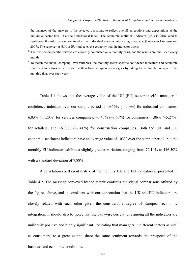
Chapter 4: Corporate Decisions, Managerial Confidence and Economic Sentiment
– 220 –
the balances of the answers to the selected questions, to reflect overall perceptions and expectations at the individual sector level in a one-dimensional index. The economic sentiment indicator (ESI) is formulated to synthesise the information contained in the individual surveys into a single variable (European Commission, 2007). The superscript (UK or EU) indicates the economy that the indicator tracks.
b. The five sector-specific surveys are currently conducted on a monthly basis, and the results are published every month.
c. To match the annual company-level variables, the monthly sector-specific confidence indicators and economic sentiment indicators are converted to their lower-frequency analogues by taking the arithmetic average of the monthly data over each year.
Table 4.1 shows that the average value of the UK (EU) sector-specific managerial
confidence indicator over our sample period is –9.56% (–4.49%) for industrial companies,
6.83% (11.20%) for services companies, –5.45% (–8.60%) for consumers, 1.86% (–5.27%)
for retailers, and –6.73% (–7.41%) for construction companies. Both the UK and EU
economic sentiment indicators have an average value of 103% over the sample period, but the
monthly EU indicator exhibits a slightly greater variation, ranging from 72.10% to 116.50%
with a standard deviation of 7.88%.
A correlation coefficient matrix of the monthly UK and EU indicators is presented in
Table 4.2. The message conveyed by the matrix confirms the visual comparisons offered by
the figures above, and is consistent with our expectation that the UK and EU indicators are
closely related with each other given the considerable degree of European economic
integration. It should also be noted that the pair-wise correlations among all the indicators are
uniformly positive and highly significant, indicating that managers in different sectors as well
as consumers, to a great extent, share the same sentiment towards the prospects of the
business and economic conditions.
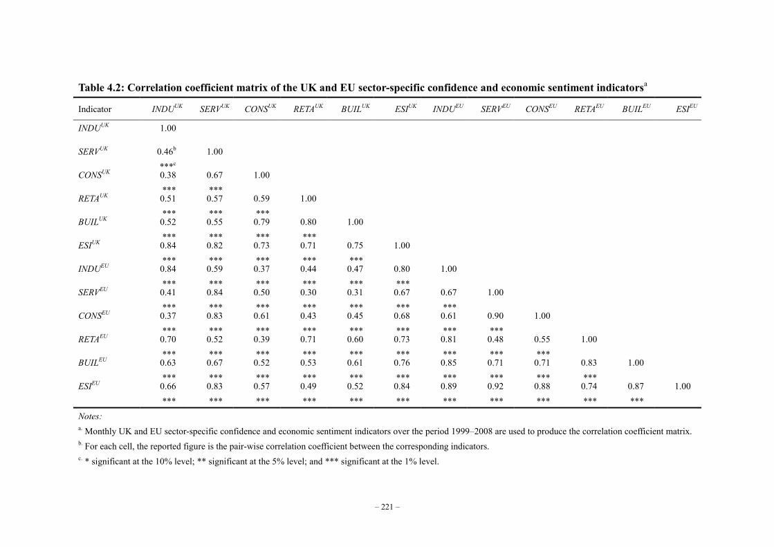
– 221 –
Table 4.2: Correlation coefficient matrix of the UK and EU sector-specific confidence and economic sentiment indicatorsa
Indicator INDUUK SERVUK CONSUK RETAUK BUILUK ESIUK INDUEU SERVEU CONSEU RETAEU BUILEU ESIEU
INDUUK 1.00
SERVUK 0.46b ***c
1.00
CONSUK 0.38 ***
0.67 ***
1.00
RETAUK 0.51 ***
0.57 ***
0.59 ***
1.00
BUILUK 0.52 ***
0.55 ***
0.79 ***
0.80 ***
1.00
ESIUK 0.84 ***
0.82 ***
0.73 ***
0.71 ***
0.75 ***
1.00
INDUEU 0.84 ***
0.59 ***
0.37 ***
0.44 ***
0.47 ***
0.80 ***
1.00
SERVEU 0.41 ***
0.84 ***
0.50 ***
0.30 ***
0.31 ***
0.67 ***
0.67 ***
1.00
CONSEU 0.37 ***
0.83 ***
0.61 ***
0.43 ***
0.45 ***
0.68 ***
0.61 ***
0.90 ***
1.00
RETAEU 0.70 ***
0.52 ***
0.39 ***
0.71 ***
0.60 ***
0.73 ***
0.81 ***
0.48 ***
0.55 ***
1.00
BUILEU 0.63 ***
0.67 ***
0.52 ***
0.53 ***
0.61 ***
0.76 ***
0.85 ***
0.71 ***
0.71 ***
0.83 ***
1.00
ESIEU 0.66 ***
0.83 ***
0.57 ***
0.49 ***
0.52 ***
0.84 ***
0.89 ***
0.92 ***
0.88 ***
0.74 ***
0.87 ***
1.00
Notes: a. Monthly UK and EU sector-specific confidence and economic sentiment indicators over the period 1999–2008 are used to produce the correlation coefficient matrix. b. For each cell, the reported figure is the pair-wise correlation coefficient between the corresponding indicators. c. * significant at the 10% level; ** significant at the 5% level; and *** significant at the 1% level.

Chapter 4: Corporate Decisions, Managerial Confidence and Economic Sentiment
– 222 –
Although the managerial confidence indicators and the economic sentiment indicators
drawn from the EU business and consumer surveys represent the combination of managerial
confidence at aggregate levels, we can still use the term managerial overconfidence or
optimism in this chapter, given the argument that the vast majority of managers provide
responses which could be considered as overconfident on any reasonable scales (Ben-David et
al., 2007).43 Oliver and Mefteh (2010) use the same set of indicators as proxies for
managerial overconfidence to investigate the influence of managers’ psychological bias on
capital structure choice with reference to a panel of French companies.
4.3 Modelling corporate behavioural equations
4.3.1 Corporate behavioural equations with proxy for the state of confidence
This chapter incorporates managerial confidence and economic sentiment into corporate
finance issues to investigate their impact on corporate investment, financing and payout
decisions. To explicitly allow for the contemporaneous interactions among the key set of
corporate decisions, we model companies’ capital investment, debt financing and dividend
payout behaviour endogenously within the simultaneous equations system set up in Chapter 3.
Given the potential influences of managers’ psychological bias on aspects of corporate
behaviour, we treat the state of confidence as a common factor involved in each of the
decisions modelled in our simultaneous system. Therefore, the simultaneous equations system
43 This is a crude approximation of managerial overconfidence, however given the data this is the best we would do.
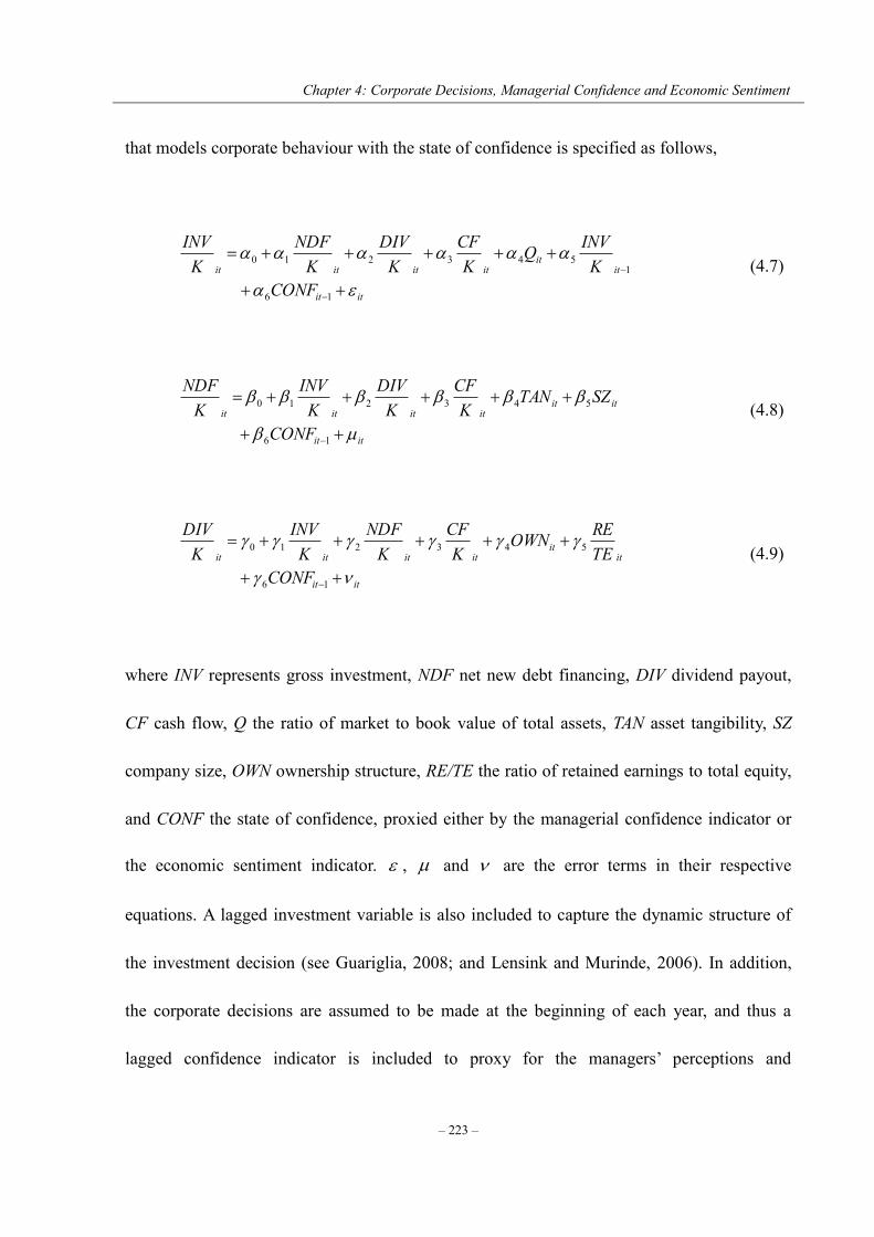
Chapter 4: Corporate Decisions, Managerial Confidence and Economic Sentiment
– 223 –
that models corporate behaviour with the state of confidence is specified as follows,
itit
itit
itititit
CONFK
INVQK
CFK
DIVK
NDFK
INV
16
1543210
(4.7)
itit
itititititit
CONF
SZTANK
CFK
DIVK
INVK
NDF
16
543210
(4.8)
itit
itit
itititit
CONFTEREOWN
KCF
KNDF
KINV
KDIV
16
543210
(4.9)
where INV represents gross investment, NDF net new debt financing, DIV dividend payout,
CF cash flow, Q the ratio of market to book value of total assets, TAN asset tangibility, SZ
company size, OWN ownership structure, RE/TE the ratio of retained earnings to total equity,
and CONF the state of confidence, proxied either by the managerial confidence indicator or
the economic sentiment indicator. , and are the error terms in their respective
equations. A lagged investment variable is also included to capture the dynamic structure of
the investment decision (see Guariglia, 2008; and Lensink and Murinde, 2006). In addition,
the corporate decisions are assumed to be made at the beginning of each year, and thus a
lagged confidence indicator is included to proxy for the managers’ perceptions and
Chapter 4: Corporate Decisions, Managerial Confidence and Economic Sentiment
– 224 –
expectations of future economic conditions when they make corporate decisions at the
beginning of each fiscal year for the year ahead, i.e. managers form their perceptions and
expectations at the beginning of the year t (or end of year t–1) according to the information set
available, and then decide how to finance and allocate their funds for year t. All the corporate
decision and cash flow variables are scaled by beginning-of-period capital stock (K), in order
to control for company size and to reduce heteroscedasticity problems that may otherwise
arise in the company-level data.
According to the behavioural corporate finance literature, managerial overconfidence
induces an underinvestment-overinvestment trade-off (see Heaton, 2002). If managers
systematically overestimate future returns to their investment projects and thus overinvest, we
expect the coefficient on the confidence variable in the investment equation to be positive. If
managers consistently perceive their companies are undervalued by the capital market and
thus are reluctant to access external finance, resulting in underinvestment, then we expect the
coefficient on the confidence variable in Equation 4.7 to be negative. The overall effect of
managerial confidence on corporate investment, therefore, is subject to empirical
examination.
The prediction with respect to managerial confidence on corporate debt financing
decision is also theoretically ambiguous. If managers have an upward bias towards future
profitability and a downward bias towards the riskiness of future earnings, we expect the
coefficient on the confidence variable in the debt financing equation to be positive. If
Chapter 4: Corporate Decisions, Managerial Confidence and Economic Sentiment
– 225 –
managers consistently perceive their company as undervalued by the capital market, and
external finance as unduly costly, we expect the coefficient on the confidence variable in
Equation 4.8 to be negative. Thus, managers’ psychological bias in relation to corporate debt
financing decisions also needs to be addressed empirically.
Again, the relationship between the state of confidence and dividend payout is also not
clear-cut. If managers are more confident about future cash flow and hence view dividend
payout as more sustainable, we expect the coefficient on the confidence variable in the
dividend payout equation to be positive. If managers overestimate both returns to investment
and costs of external finance, and therefore view internally generated cash flows as more
valuable, we expect managerial confidence in Equation 4.9 to have a negative effect on
dividend payouts.
Equations 4.7 through 4.9 form a simultaneous equations system, in which corporate
decisions are jointly determined by managers based on their confidence towards future
company performance. We employ two proxies for the state of confidence (CONF), i.e. a
sector-specific managerial confidence indicator (SCI) and economic sentiment indicator (ESI),
as described in Section 4.3. Both indicators are measured at two levels, i.e. the UK country
level (SCIUK and ESIUK) and the EU regional level (SCIEU and ESIEU). The candidate
indicators are used as the confidence variable separately in their respective simultaneous
equations system variants. Industry dummies are included in all of the equations to account
for inter-industry variations that cannot be captured by the included regressors. We do not

Chapter 4: Corporate Decisions, Managerial Confidence and Economic Sentiment
– 226 –
include year dummies in our equations because the variables employed to proxy for the state
of confidence and sentiment in this chapter are all at aggregate levels, and their effects on
corporate decisions may, to some extent, be captured by the year dummies.
4.3.2 Corporate behavioural equations with confidence and uncertainty variables
Recent literature in corporate finance has also recognised the importance of uncertainty
associated with companies’ prospects in the determination of corporate decisions (see the
literature reviewed in Section 2.4). Chapter 3 of this thesis also pays great attention to the
impacts of uncertainty at company level on jointly determined corporate investment,
financing and payout choices. We construct our proxies for uncertainty based on stock price
volatility, under the assumption that all the information about a company’s fundamentals and
prospects will be properly transmitted into its share price. Using a large panel of UK-listed
companies within the period 1999–2008, we find that companies are likely to increase their
investment outlays in the face of greater uncertainty. To finance the increased investment
under uncertainty, they tend to resort to internal funds by cutting dividends rather than
resorting to external funds by issuing new debts. Overall, the findings of Chapter 3 strongly
support the argument that managers do take uncertainty associated with their company’s
prospects into consideration when they make real and financial decisions.
An interesting related question is whether the state of managerial confidence and
economic sentiment towards future business performance can be adequately reflected in the
changes in share prices and empirically captured by our proxy for company-level uncertainty
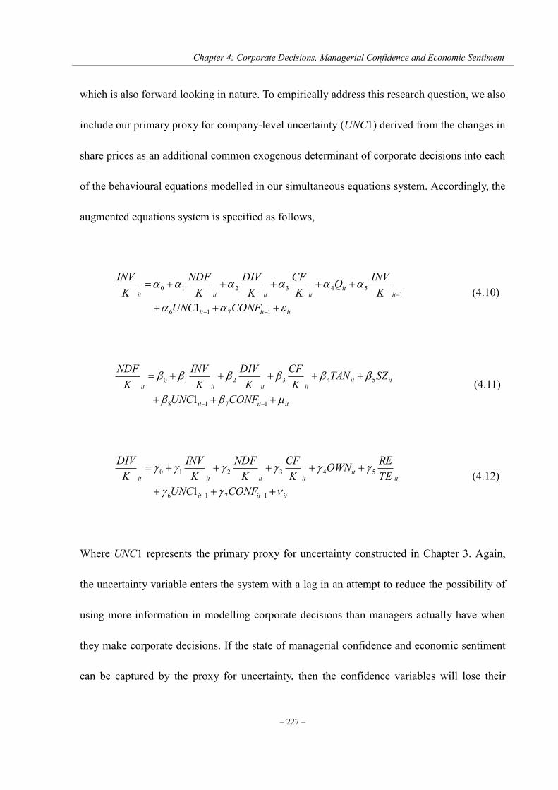
Chapter 4: Corporate Decisions, Managerial Confidence and Economic Sentiment
– 227 –
which is also forward looking in nature. To empirically address this research question, we also
include our primary proxy for company-level uncertainty (UNC1) derived from the changes in
share prices as an additional common exogenous determinant of corporate decisions into each
of the behavioural equations modelled in our simultaneous equations system. Accordingly, the
augmented equations system is specified as follows,
ititit
itit
itititit
CONFUNCK
INVQK
CFK
DIVK
NDFK
INV
1716
1543210
1 (4.10)
ititit
itititititit
CONFUNC
SZTANK
CFK
DIVK
INVK
NDF
1718
543210
1 (4.11)
ititit
itit
itititit
CONFUNCTEREOWN
KCF
KNDF
KINV
KDIV
1716
543210
1 (4.12)
Where UNC1 represents the primary proxy for uncertainty constructed in Chapter 3. Again,
the uncertainty variable enters the system with a lag in an attempt to reduce the possibility of
using more information in modelling corporate decisions than managers actually have when
they make corporate decisions. If the state of managerial confidence and economic sentiment
can be captured by the proxy for uncertainty, then the confidence variables will lose their
Chapter 4: Corporate Decisions, Managerial Confidence and Economic Sentiment
– 228 –
explanatory powers for corporate decisions once the company-level uncertainty is
incorporated in the system. On the other hand, if the confidence variables do indeed hold
additional information useful in explaining corporate behaviour, their explanatory powers are
expected to persist even after controlling for company-level uncertainty.
4.4 Data and preliminary analysis
Our data are collected from the Worldscope database via Thomson One Banker Analytics. The
initial sample includes all companies listed on the London Stock Exchange (LSE), including
both active and inactive companies, within the period 1999–2008. We then discard utilities
(SIC code 4900–4949), and financial companies (SIC code 6000–6999). Companies that do
not have complete records on all the relevant variables in determining corporate investment,
financing and payout decisions as well as those with less than five years of continuous
observations are dropped from our sample. We also exclude company-year observations with
negative cash flow from our sample. The number of company-year observations included in
the final sample for the simultaneous equations analyses therefore reduces to 2,791. The
indicators for managerial confidence and economic sentiment at UK level and EU level are
publicly available from the European Commission website. An unbalanced panel of
company-level data, therefore, is formed to avoid survivorship bias and to make full use of the
company-year observations. The measurement of each variable used in this chapter is
described in Table 4.3.
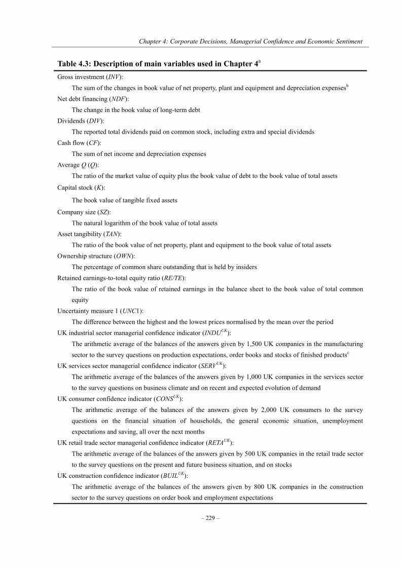
Chapter 4: Corporate Decisions, Managerial Confidence and Economic Sentiment
– 229 –
Table 4.3: Description of main variables used in Chapter 4a Gross investment (INV):
The sum of the changes in book value of net property, plant and equipment and depreciation expensesb Net debt financing (NDF):
The change in the book value of long-term debt Dividends (DIV):
The reported total dividends paid on common stock, including extra and special dividends Cash flow (CF):
The sum of net income and depreciation expenses Average Q (Q):
The ratio of the market value of equity plus the book value of debt to the book value of total assets
Capital stock (K):
The book value of tangible fixed assets
Company size (SZ): The natural logarithm of the book value of total assets
Asset tangibility (TAN): The ratio of the book value of net property, plant and equipment to the book value of total assets
Ownership structure (OWN): The percentage of common share outstanding that is held by insiders
Retained earnings-to-total equity ratio (RE/TE): The ratio of the book value of retained earnings in the balance sheet to the book value of total common equity
Uncertainty measure 1 (UNC1): The difference between the highest and the lowest prices normalised by the mean over the period
UK industrial sector managerial confidence indicator (INDUUK): The arithmetic average of the balances of the answers given by 1,500 UK companies in the manufacturing sector to the survey questions on production expectations, order books and stocks of finished productsc
UK services sector managerial confidence indicator (SERVUK): The arithmetic average of the balances of the answers given by 1,000 UK companies in the services sector to the survey questions on business climate and on recent and expected evolution of demand
UK consumer confidence indicator (CONSUK): The arithmetic average of the balances of the answers given by 2,000 UK consumers to the survey questions on the financial situation of households, the general economic situation, unemployment expectations and saving, all over the next months
UK retail trade sector managerial confidence indicator (RETAUK): The arithmetic average of the balances of the answers given by 500 UK companies in the retail trade sector to the survey questions on the present and future business situation, and on stocks
UK construction confidence indicator (BUILUK): The arithmetic average of the balances of the answers given by 800 UK companies in the construction sector to the survey questions on order book and employment expectations
Chapter 4: Corporate Decisions, Managerial Confidence and Economic Sentiment
– 230 –
UK sector-specific managerial confidence indicator (SCIUK): The value of the industry-wide managerial confidence in the UK for a company, which is equal to INDUUK for companies in the manufacturing sector, SERVUK for companies in the services sector, RETAUK for companies in the retail trade sector and BUILUK for companies in the construction sector
UK economic sentiment indicator (ESIUK): The indicator which is made up of 15 individual components of UK sector-specific confidence indicators to track cyclical movements in the UK economy as a whole
EU industrial sector managerial confidence indicator (INDUEU): The arithmetic average of the balances of the answers given by 38,250 EU companies in the manufacturing sector to the survey questions on production expectations, order books and stocks of finished products
EU services sector managerial confidence indicator (SERVEU): The arithmetic average of the balances of the answers given by 34,730 EU companies in the services sector to the survey questions on business climate and on recent and expected evolution of demand
EU consumer confidence indicator (CONSEU): The arithmetic average of the balances of the answers given by 39,900 EU consumers to the survey questions on the financial situation of households, the general economic situation, unemployment expectations and saving, all over the next months
EU retail trade sector managerial confidence indicator (RETAEU): The arithmetic average of the balances of the answers given by 31,780 EU companies in the retail trade sector to the survey questions on the present and future business situation, and on stocks
EU construction sector managerial confidence indicator (RETAEU): The arithmetic average of the balances of the answers given by 20,750 EU companies in the construction sector to the survey questions on order book and employment expectations
EU sector-specific managerial confidence indicator (SCIEU): The value of the industry-wide managerial confidence in the EU for a company, which is equal to INDUEU for companies in the manufacturing sector, SERVEU for companies in the services sector, RETAEU for companies in the retail trade sector and BUILEU for companies in the construction sector
EU economic sentiment indicator (ESIEU): The indicator which is made up of 15 individual components of EU sector-specific confidence indicators to track cyclical movements in the EU economy as a whole
Notes: a. The definition and measurement of the company characteristic variables are based on the existing literature. b. The data are collected from the Worldscope database via Thomson One Banker Analytics. c. The sector-specific confidence indicators and economic sentiment indicators are publicly available from the
European Commission website.
The descriptive statistics for the main variables used in this chapter, both before and
after winsorisation transformation, are presented in Table 4.4.
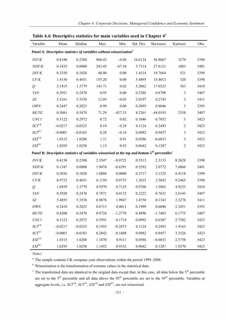
Chapter 4: Corporate Decisions, Managerial Confidence and Economic Sentiment
– 231 –
Table 4.4: Descriptive statistics for main variables used in Chapter 4a
Variable Mean Median Max. Min. Std. Dev. Skewness Kurtosis Obs.
Panel A: Descriptive statistics of variables without winsorisationb
INV/K 0.8180 0.2388 960.43 –0.96 16.6124 56.8067 3279 3398
NDF/K 0.3435 0.0000 243.45 –67.54 5.7114 27.8121 1083 3401
DIV/K 0.3250 0.1020 48.00 0.00 1.4514 19.7664 521 3399
CF/K 1.4156 0.4651 155.20 0.00 5.4895 15.4013 320 3398
Q 2.1415 1.3779 143.71 0.02 5.2062 17.0323 383 3410
TAN 0.2951 0.2470 0.95 0.00 0.2305 0.8798 3 3407
SZ 5.5161 5.3538 12.05 –0.03 2.0197 0.2745 3 3411
OWN 0.2447 0.2023 0.99 0.00 0.2093 0.8046 3 3393
RE/TE 0.3081 0.5478 71.29 –437.33 8.2261 –44.0193 2358 3407
UNC1 0.3122 0.2972 0.72 0.02 0.1046 0.7052 3 3423
SCIUK –0.0217 –0.0325 0.19 –0.29 0.1124 0.2493 2 3423
SCIEU –0.0001 –0.0183 0.28 –0.16 0.0982 0.9457 3 3423
ESIUK 1.0315 1.0288 1.11 0.91 0.0586 –0.6033 3 3423
ESIEU 1.0295 1.0258 1.15 0.93 0.0642 0.1287 2 3423
Panel B: Descriptive statistics of variables winsorised at the top and bottom 5th
percentilesc
INV/K 0.4130 0.2388 2.3547 –0.0723 0.5313 2.3133 8.2628 3398
NDF/K 0.1347 0.0000 1.9474 –0.6391 0.5292 2.0772 7.6866 3401
DIV/K 0.2036 0.1020 1.0888 0.0000 0.2717 2.1325 6.9118 3399
CF/K 0.9722 0.4651 6.1150 0.0733 1.3625 2.5842 9.2465 3398
Q 1.6939 1.3779 4.5970 0.7125 0.9760 1.5863 4.9233 3410
TAN 0.2920 0.2470 0.7871 0.0172 0.2222 0.7621 2.6143 3407
SZ 5.4855 5.3538 8.9878 1.9947 1.8750 0.1343 2.2278 3411
OWN 0.2410 0.2023 0.6713 0.0011 0.1999 0.6096 2.3451 3393
RE/TE 0.4208 0.5478 0.9724 –1.2778 0.4996 –1.7403 6.1775 3407
UNC1 0.3123 0.2972 0.5591 0.1714 0.0992 0.6307 2.7302 3423
SCIUK –0.0217 –0.0325 0.1933 –0.2875 0.1124 0.2493 1.9163 3423
SCIEU –0.0001 –0.0183 0.2842 –0.1608 0.0982 0.9457 3.3526 3423
ESIUK 1.0315 1.0288 1.1070 0.9111 0.0586 –0.6033 2.5758 3423
ESIEU 1.0295 1.0258 1.1452 0.9332 0.0642 0.1287 1.9270 3423
Notes: a. The sample contains UK company-year observations within the period 1999–2008. b. Winsorisation is the transformation of extreme values in the statistical data. c. The transformed data are identical to the original data except that, in this case, all data below the 5th percentile
are set to the 5th percentile and all data above the 95th percentile are set to the 95th percentile. Variables at
aggregate levels, i.e. SCIUK, SCIEU, ESIUK and ESIEU, are not winsorised.
Chapter 4: Corporate Decisions, Managerial Confidence and Economic Sentiment
– 232 –
Panel A in Table 4.4 presents the descriptive statistics for the main variables from our
raw data. As is evident, extreme values appear in almost all the variables, especially those that
are in the form of ratios. In order to cope with the potential impact of outliers upon our
empirical tests, we winsorise all the company-level variables used in our analysis at both the
top and bottom 5th percentiles of their respective distributions. Panel B in Table 4.4 reports the
descriptive statistics after such a transformation has been undertaken. Since the proxies for
managerial confidence and economic sentiment are at aggregated levels, we do not winsorise
them. Given the desired properties of the winsorisation estimators, our empirical results
presented this chapter are based on the variables winsorised at both the top and bottom 5th
percentiles.
A pair-wise correlation among the main variables is presented in Table 4.5. It shows
that the three endogenous variables, namely, INV/K, NDF/K and DIV/K, are significantly and
positively correlated with one another, and that the predetermined cash flow variable CF/K is
significantly correlated with all three endogenous variables. It is also evident that the
managerial confidence and economic sentiment variables, namely, SCIUK, SCIEU, ESIUK and
ESIEU, are significantly correlated with all three corporate decisions variables at the 1%
significance level. The correlations between the confidence variables and corporate decisions
variables are uniformly positive, indicating capital investment and debt financing as well as
dividend payouts of UK-listed companies are likely to increase with the level of managerial
confidence and economic sentiment.
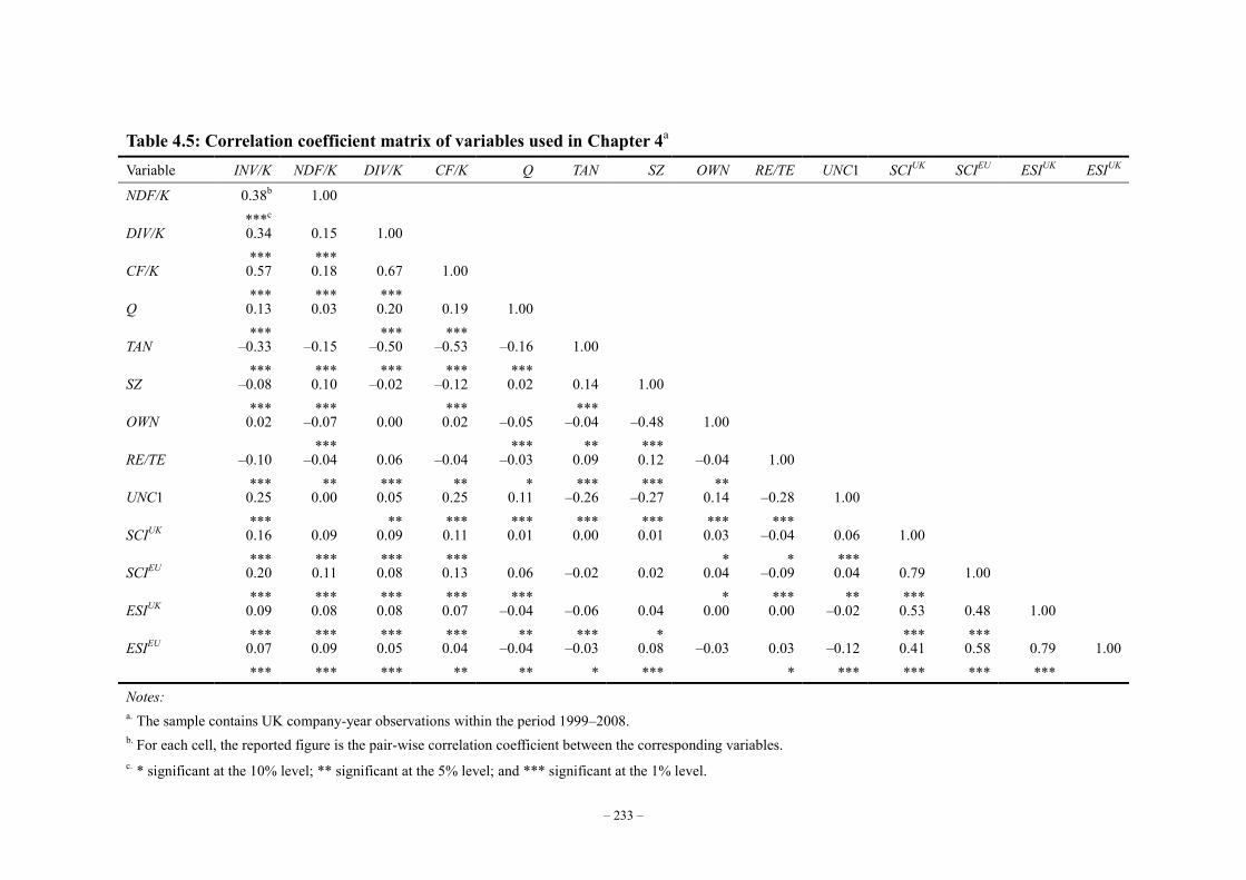
– 233 –
Table 4.5: Correlation coefficient matrix of variables used in Chapter 4a Variable INV/K NDF/K DIV/K CF/K Q TAN SZ OWN RE/TE UNC1 SCIUK SCIEU ESIUK ESIUK
NDF/K 0.38b ***c
1.00
DIV/K 0.34 ***
0.15 ***
1.00
CF/K 0.57 ***
0.18 ***
0.67 ***
1.00
Q 0.13 ***
0.03
0.20 ***
0.19 ***
1.00
TAN –0.33 ***
–0.15 ***
–0.50 ***
–0.53 ***
–0.16 ***
1.00
SZ –0.08 ***
0.10 ***
–0.02
–0.12 ***
0.02
0.14 ***
1.00
OWN 0.02
–0.07 ***
0.00
0.02
–0.05 ***
–0.04 **
–0.48 ***
1.00
RE/TE –0.10 ***
–0.04 **
0.06 ***
–0.04 **
–0.03 *
0.09 ***
0.12 ***
–0.04 **
1.00
UNC1 0.25 ***
0.00
0.05 **
0.25 ***
0.11 ***
–0.26 ***
–0.27 ***
0.14 ***
–0.28 ***
1.00
SCIUK 0.16 ***
0.09 ***
0.09 ***
0.11 ***
0.01
0.00
0.01
0.03 *
–0.04 *
0.06 ***
1.00
SCIEU 0.20 ***
0.11 ***
0.08 ***
0.13 ***
0.06 ***
–0.02
0.02
0.04 *
–0.09 ***
0.04 **
0.79 ***
1.00
ESIUK 0.09 ***
0.08 ***
0.08 ***
0.07 ***
–0.04 **
–0.06 ***
0.04 *
0.00
0.00
–0.02
0.53 ***
0.48 ***
1.00
ESIEU 0.07 ***
0.09 ***
0.05 ***
0.04 **
–0.04 **
–0.03 *
0.08 ***
–0.03
0.03 *
–0.12 ***
0.41 ***
0.58 ***
0.79 ***
1.00
Notes: a. The sample contains UK company-year observations within the period 1999–2008. b. For each cell, the reported figure is the pair-wise correlation coefficient between the corresponding variables. c. * significant at the 10% level; ** significant at the 5% level; and *** significant at the 1% level.
Chapter 4: Corporate Decisions, Managerial Confidence and Economic Sentiment
– 234 –
The correlations between the endogenous variables and other relevant exogenous
variables are also informative. According to Table 4.5, INV/K is significantly and positively
correlated with Q and UNC1; NDF/K is positively correlated with SZ but negatively
correlated with TAN; DIV/K is positively correlated with RE/TE and UNC1, but its correlation
with OWN is rather weak. Besides, the proxy for company-level uncertainty UNC1 is
positively correlated with the sector-specific managerial confidence indicators SCIUK and
SCIEU, negatively correlated with the overall economic sentiment indicators ESIUK and ESIEU.
In addition, there is no evidence of near multicollinearity presented in the correlation
coefficient matrix. Although the proxies for the state of managerial confidence and economic
sentiment are highly correlated with one another (both the correlation coefficient between
SCIUK and SCIEU and that between ESIUK and ESIEU are as high as 0.79), they do not cause the
problem of multicollinearity since they do not enter the corporate behavioural equations at the
same time. Instead, we include the alternative proxies for managerial confidence and
economic sentiment into their respective system variants separately.
4.5 Empirical results and implications for corporate behaviour
To obtain our main empirical results, we apply the 3SLS estimation to all the simultaneous
equations system variants that include one structural equation for each of the three policy
choices specified in Section 4.3. The essential advantage of the 3SLS estimation technique is
that it allows for not only simultaneity among the set of corporate decisions, but also for
correlations among the error components. Therefore, 3SLS estimation is asymptotically more

Chapter 4: Corporate Decisions, Managerial Confidence and Economic Sentiment
– 235 –
efficient than the limited information methods, such as 2SLS estimation.
We test the significance of the confidence variables within an individual equation as
well as across all equations in the system using the Wald test.44 The null hypothesis is that the
confidence variable or the set of confidence variables does not help in explaining the
variations in the corresponding corporate decision variable, and thus can be dropped from the
equation. If the null hypothesis is rejected, it means that the managerial confidence or
economic sentiment in fact plays a role in the determination of the corresponding corporate
decision.45
The same test is also carried out to test the joint significance of a confidence variable
in all corporate behavioural equations modelled in the system. The null hypothesis for the
cross-equation test is that the coefficients on the confidence variable in all equations in which
it appears are jointly equal to zero. In other words, under the null hypothesis, the confidence
variable being tested does not contain useful information which can help in explaining any
aspect of corporate behaviour, and hence should be excluded from the simultaneous equations
system. If the composite hypothesis is rejected, the presence of the confidence variable in the
system is justified, suggesting that modelling corporate behaviour without considering the
state of managerial confidence or economic sentiment is economically incomplete and
statistically inadequate.
44 These test statistics are asymptotically distributed as Chi-squared. 45 The Wald test result is identical to the corresponding z-statistic reported in the regression results, if there is only one coefficient under test.
Chapter 4: Corporate Decisions, Managerial Confidence and Economic Sentiment
– 236 –
4.5.1 Simultaneous analyses with proxy for the state of confidence
Table 4.6 reports the empirical results by applying the 3SLS estimation to Equations 4.7–4.9,
where the managerial confidence indicators SCIUK and SCIEU are used as the proxy for the
state of confidence in their respective system variants. The regression results for the
investment, financing and payout equations, in which the UK managerial confidence indicator
is used, are presented in columns 2, 4 and 6, respectively.
Looking first at the investment equation, it is evident that the coefficients on the two
endogenous explanatory variables, i.e. NDF/K and DIV/K, are both significant at the 5%
significance level. The significantly positive relationship between investment and dividend
variables evidenced in the simple pair-wise correlation analysis is reversed to be significantly
negative when the full structural investment equation is estimated within the simultaneous
equations system, suggesting that they represent competing uses of limited funds. The
coefficient on the cash flow variable CF/K is positive and highly significant as expected. The
significantly positive effect of internally generated cash flow further confirms that UK-listed
companies are financially constrained, and thus their investments display high sensitivity to
the availability of internal funds. More importantly, the proxy for the UK managerial
confidence SICUK in the investment equation turns out to be positive and highly significant at
the 1% significance level, after controlling for the set of company fundamental variables
which, according to the existing literature, are the primary determinants of corporate
investment. It appears that UK-listed companies tend to invest more intensively in their
Chapter 4: Corporate Decisions, Managerial Confidence and Economic Sentiment
– 237 –
capital stock when their managers are more confident, or possibly overconfident, about the
future company performance. This is consistent with the theoretical predictions made by
Heaton (2002) and empirical findings offered by Ben-David et al. (2007) that overconfident
managers systematically overestimate the returns to their investment projects, and
simultaneously underestimate the risks associated with those projects, resulting in unintended
overinvestment and risk-taking behaviour. Besides, the proxy for investment opportunity Q is
positively related to the investment variable, but not statistically significant at the
conventional levels. The dynamic structure of corporate investment is statistically evident.
Turing to the financing regression reported in column 4 of Table 4.6, the coefficients
on the endogenous variables INV/K and DIV/K are both positive and marginally significant,
while the coefficient on the cash flow variable CF/K is negative and highly significant, as
predicted by the flow-of-funds framework. These findings are in line with the hierarchy of
raising funds as implied by the pecking-order theory. The coefficient on the UK managerial
confidence indicator SICUK turns out to be positive and statistically significant at the 1% level.
It shows that managerial confidence or overconfidence is an important factor in explaining
corporate debt financing behaviour, even after controlling for the major conventional capital
structure determinants. Managerial confidence is clearly associated with aggressive borrowing
policies of the UK-listed companies, implying that managers tend to overestimate their
companies’ growth rate of earnings and underestimate the associated risks when they are more
confident, and thus use debt financing more aggressively. Our finding is consistent with the
Chapter 4: Corporate Decisions, Managerial Confidence and Economic Sentiment
– 238 –
prior studies on managerial overconfidence and corporate financial policies, for example
Hackbarth (2008), Ben-David et al. (2007) and Malmendier et al. (2011). We do not find
evidence that overconfident managers view external funds as unduly costly and are reluctant
to raise funds externally. The results for the control variables are similar to those reported in
Chapter 3 that the effect of company size SZ is highly significant as expected, whist the effect
of asset tangibility TAN is also significant but with an unexpected sign.
Column 6 of Table 4.6 reports the estimation results for the dividend payout regression.
The coefficients estimated for the endogenous variables INV/K and NDF/K as well as the
predetermined cash flow variable CF/K have their expected signs and are highly significant at
the 1% level, which further confirms the simultaneity among the key set of corporate
decisions. The payout decisions of the UK-listed companies are neither totally residual nor
entirely independent but are taken with reference to their investment and financing decisions.
However, the effect of managerial confidence on corporate payout decisions is relatively weak.
Although the coefficient on the managerial confidence variable SCIUK is not significant at the
usual significance levels, its negative sign implies that confident managers may have a
stronger preference for internal funds and are more likely to retain internally generated cash
flows in an attempt to finance their investment opportunities at a lower cost. Besides, the
ownership structure and the financial life cycle stage variables (OWN and RE/TE) are both
positively related to corporate payout decisions, and the highly significant coefficient on
RE/TE is consistent with the predictions of the life cycle theory of dividend payout.
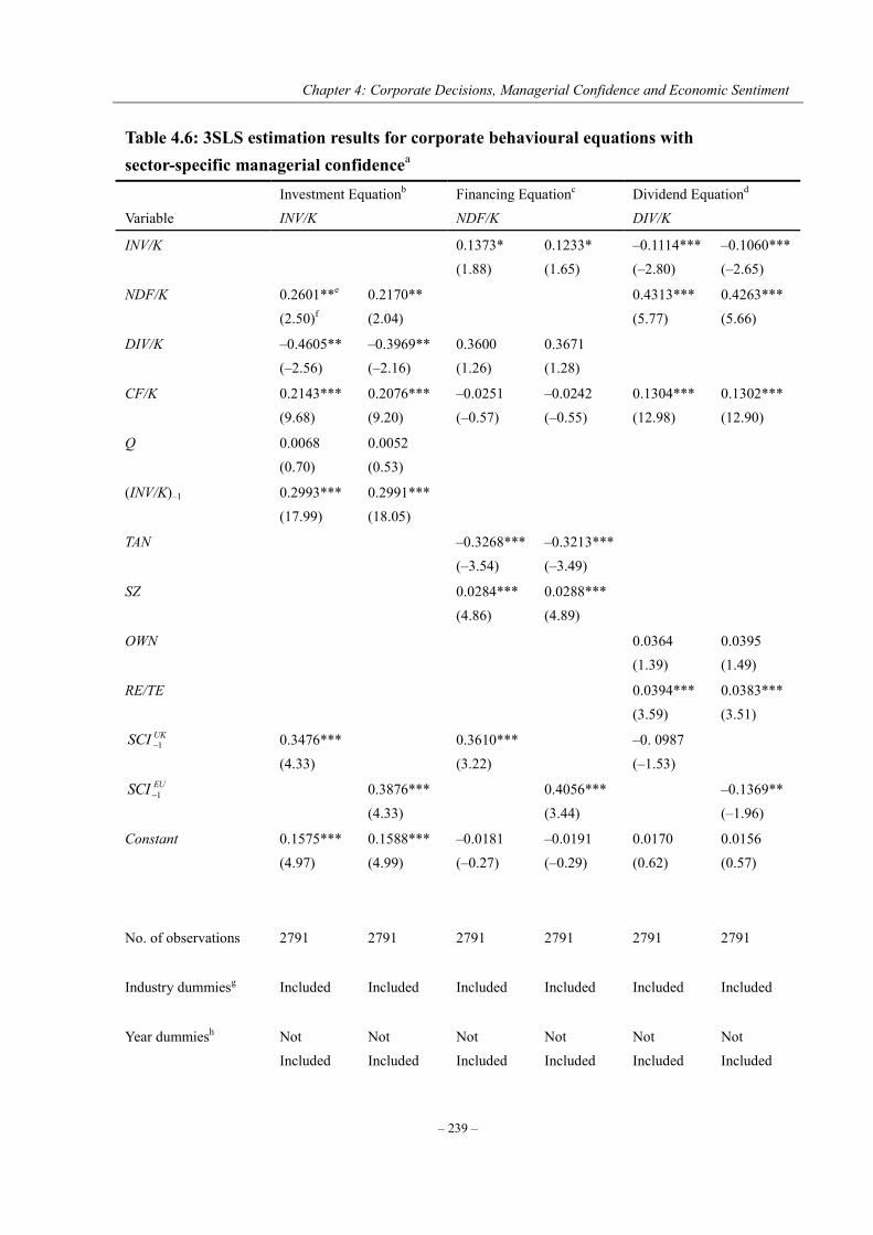
Chapter 4: Corporate Decisions, Managerial Confidence and Economic Sentiment
– 239 –
Table 4.6: 3SLS estimation results for corporate behavioural equations with sector-specific managerial confidencea
Variable Investment Equationb INV/K
Financing Equationc NDF/K
Dividend Equationd DIV/K
INV/K 0.1373* (1.88)
0.1233* (1.65)
–0.1114*** (–2.80)
–0.1060*** (–2.65)
NDF/K 0.2601**e (2.50)f
0.2170** (2.04)
0.4313*** (5.77)
0.4263*** (5.66)
DIV/K –0.4605** (–2.56)
–0.3969** (–2.16)
0.3600 (1.26)
0.3671 (1.28)
CF/K 0.2143*** (9.68)
0.2076*** (9.20)
–0.0251 (–0.57)
–0.0242 (–0.55)
0.1304*** (12.98)
0.1302*** (12.90)
Q 0.0068 (0.70)
0.0052 (0.53)
(INV/K)–1 0.2993*** (17.99)
0.2991*** (18.05)
TAN –0.3268*** (–3.54)
–0.3213*** (–3.49)
SZ 0.0284*** (4.86)
0.0288*** (4.89)
OWN 0.0364 (1.39)
0.0395 (1.49)
RE/TE 0.0394*** (3.59)
0.0383*** (3.51)
UKSCI 1 0.3476*** (4.33)
0.3610*** (3.22)
–0. 0987 (–1.53)
EUSCI 1 0.3876*** (4.33)
0.4056*** (3.44)
–0.1369** (–1.96)
Constant 0.1575*** (4.97)
0.1588*** (4.99)
–0.0181 (–0.27)
–0.0191 (–0.29)
0.0170 (0.62)
0.0156 (0.57)
No. of observations
2791 2791 2791 2791 2791 2791
Industry dummiesg
Included Included Included Included Included Included
Year dummiesh
Not Included
Not Included
Not Included
Not Included
Not Included
Not Included
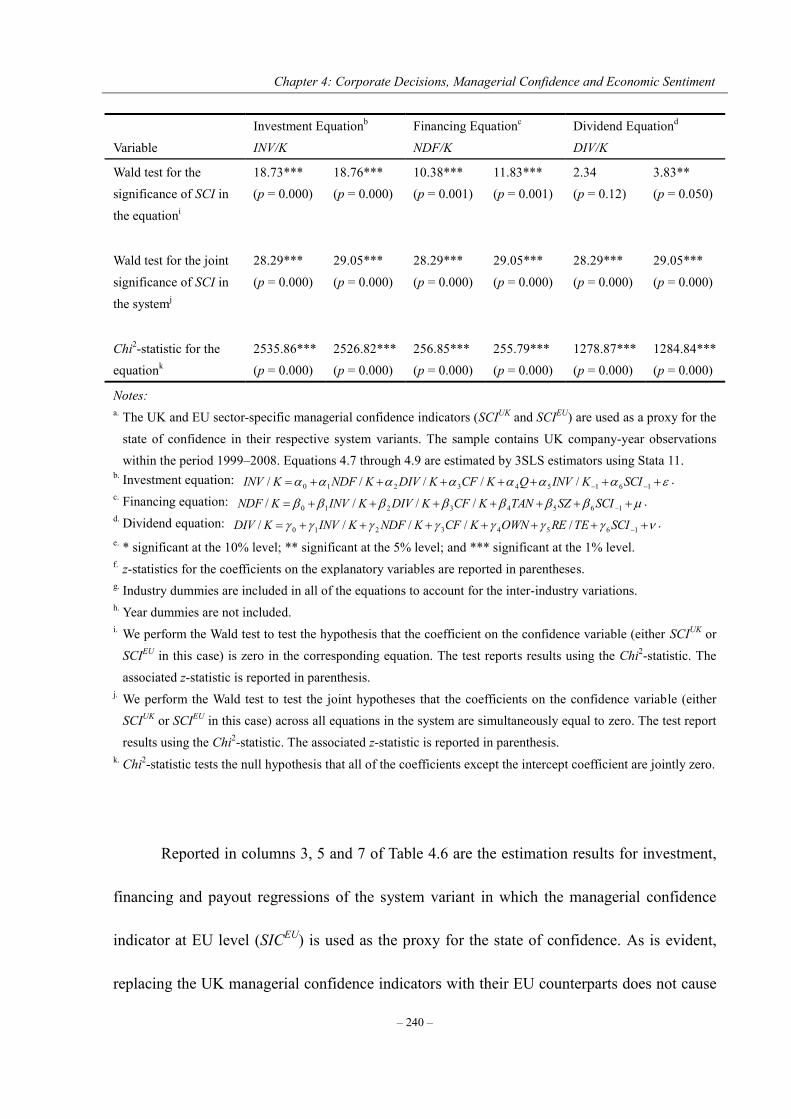
Chapter 4: Corporate Decisions, Managerial Confidence and Economic Sentiment
– 240 –
Variable Investment Equationb INV/K
Financing Equationc NDF/K
Dividend Equationd DIV/K
Wald test for the significance of SCI in the equationi
18.73*** (p = 0.000)
18.76*** (p = 0.000)
10.38*** (p = 0.001)
11.83*** (p = 0.001)
2.34 (p = 0.12)
3.83** (p = 0.050)
Wald test for the joint significance of SCI in the systemj
28.29*** (p = 0.000)
29.05*** (p = 0.000)
28.29*** (p = 0.000)
29.05*** (p = 0.000)
28.29*** (p = 0.000)
29.05*** (p = 0.000)
Chi2-statistic for the equationk
2535.86*** (p = 0.000)
2526.82*** (p = 0.000)
256.85*** (p = 0.000)
255.79*** (p = 0.000)
1278.87*** (p = 0.000)
1284.84*** (p = 0.000)
Notes: a. The UK and EU sector-specific managerial confidence indicators (SCIUK and SCIEU) are used as a proxy for the
state of confidence in their respective system variants. The sample contains UK company-year observations within the period 1999–2008. Equations 4.7 through 4.9 are estimated by 3SLS estimators using Stata 11.
b. Investment equation: 161543210 ///// SCIKINVQKCFKDIVKNDFKINV . c. Financing equation: 16543210 //// SCISZTANKCFKDIVKINVKNDF . d. Dividend equation: 16543210 ///// SCITEREOWNKCFKNDFKINVKDIV . e. * significant at the 10% level; ** significant at the 5% level; and *** significant at the 1% level. f. z-statistics for the coefficients on the explanatory variables are reported in parentheses. g. Industry dummies are included in all of the equations to account for the inter-industry variations. h. Year dummies are not included. i. We perform the Wald test to test the hypothesis that the coefficient on the confidence variable (either SCIUK or
SCIEU in this case) is zero in the corresponding equation. The test reports results using the Chi2-statistic. The associated z-statistic is reported in parenthesis.
j. We perform the Wald test to test the joint hypotheses that the coefficients on the confidence variable (either SCIUK or SCIEU in this case) across all equations in the system are simultaneously equal to zero. The test report results using the Chi2-statistic. The associated z-statistic is reported in parenthesis.
k. Chi2-statistic tests the null hypothesis that all of the coefficients except the intercept coefficient are jointly zero.
Reported in columns 3, 5 and 7 of Table 4.6 are the estimation results for investment,
financing and payout regressions of the system variant in which the managerial confidence
indicator at EU level (SICEU) is used as the proxy for the state of confidence. As is evident,
replacing the UK managerial confidence indicators with their EU counterparts does not cause
Chapter 4: Corporate Decisions, Managerial Confidence and Economic Sentiment
– 241 –
significant changes in our results. However, the coefficient on the managerial confidence
variable SICEU in the payout equation (see column 7) turns out to be negative and statistically
significant. It seems that the dividend payout policies of the UK-listed companies are more
likely to be influenced by the collective managerial confidence and sentiment at higher levels
of aggregation. In accordance with the prediction of managerial psychological bias,
overconfident managers misperceive the profitability of their investment opportunities as well
as the value of their companies. Consequently, they tend to overinvest in projects whose net
present values are possibly overestimated, resulting in higher financing needs. Meanwhile,
they also try to avoid external financing which is possibly misperceived as unduly costly.
Under such circumstances, overconfident managers view internal funds as more valuable and
have a stronger preference for internal financing. Therefore, managers are likely to retain
more internally generated cash flow when they are more confident, in order to prevent losses
from underinvestment, and to keep their overall cost of capital as low as possible. Besides, the
Wald test results reported at the bottom of Table 4.6 strongly suggest that our proxies for
managerial confidence do indeed play an important role in the determination of the corporate
decisions. Therefore, modelling corporate behaviour using company fundamental
characteristics without considering the state of managerial confidence is incomplete.
An alternative measure of the state of confidence used in this chapter is the economic
sentiment indicator (ESI). The UK economic sentiment indicator (ESIUK) and the EU
economic sentiment indicator (ESIEU) are employed in their respective system variants, and
Chapter 4: Corporate Decisions, Managerial Confidence and Economic Sentiment
– 242 –
the 3SLS estimation results are reported in Table 4.7. The regression results obtained by using
the economic sentiment indicator as the proxy for the state of confidence are similar to those
reported in Table 4.6 in the terms of the significance levels and the sizes of the coefficients for
the confidence variable as well as the control variables. First, the coefficients on the
endogenous explanatory variables are not only statistically significant but also economically
meaningful, which lends strong empirical support to the prediction of the flow-of-funds
framework that corporate investment, financing and payout decisions are simultaneously
determined by the UK-listed companies. The UK economic sentiment indicator (ESIUK) enters
both the investment equation and the financing equation with a positive sign, and is
statistically significant in both equations, indicating that UK-listed companies invest in capital
stock more intensively and use debt more aggressively when the economic sentiment in the
UK is high. The UK economic sentiment indicator enters the payout equation with a negative
sign but its influence on dividend payout decisions of UK companies is rather weak.
Compared with the UK economic sentiment indicator, its EU counterpart (ESIEU) seems to be
better able to explain the debt financing and dividend payout decisions of UK companies,
while it provides less explanatory power for corporate investment decisions. The Wald test
results exhibit high joint significance of the economic sentiment variables in their respective
system variants. In summary, our results for both managerial confidence and economic
sentiment are statistically significant, particularly in explaining the corporate investment and
debt financing decisions of UK-listed companies.
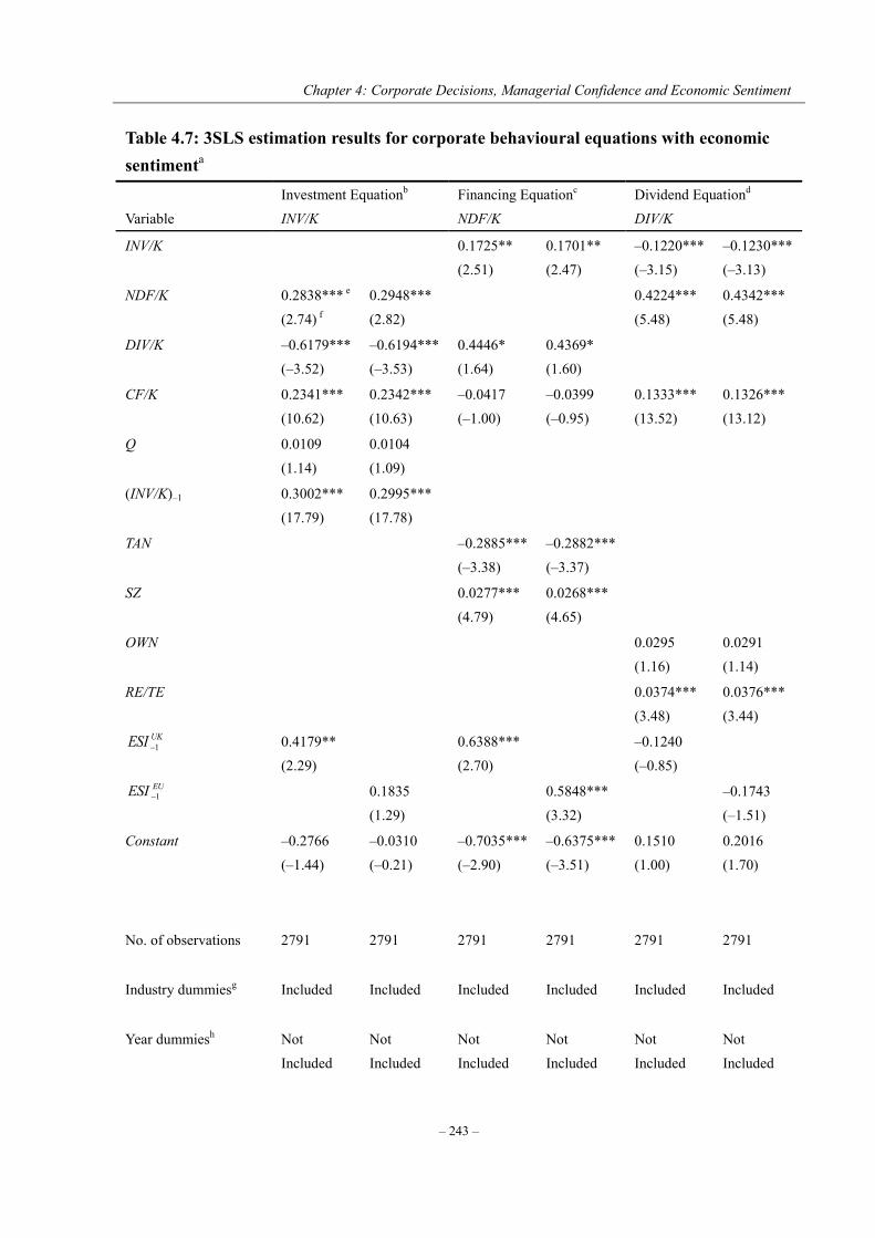
Chapter 4: Corporate Decisions, Managerial Confidence and Economic Sentiment
– 243 –
Table 4.7: 3SLS estimation results for corporate behavioural equations with economic sentimenta
Variable Investment Equationb INV/K
Financing Equationc NDF/K
Dividend Equationd DIV/K
INV/K 0.1725** (2.51)
0.1701** (2.47)
–0.1220*** (–3.15)
–0.1230*** (–3.13)
NDF/K 0.2838*** e (2.74) f
0.2948*** (2.82)
0.4224*** (5.48)
0.4342*** (5.48)
DIV/K –0.6179*** (–3.52)
–0.6194*** (–3.53)
0.4446* (1.64)
0.4369* (1.60)
CF/K 0.2341*** (10.62)
0.2342*** (10.63)
–0.0417 (–1.00)
–0.0399 (–0.95)
0.1333*** (13.52)
0.1326*** (13.12)
Q 0.0109 (1.14)
0.0104 (1.09)
(INV/K)–1 0.3002*** (17.79)
0.2995*** (17.78)
TAN –0.2885*** (–3.38)
–0.2882*** (–3.37)
SZ 0.0277*** (4.79)
0.0268*** (4.65)
OWN 0.0295 (1.16)
0.0291 (1.14)
RE/TE 0.0374*** (3.48)
0.0376*** (3.44)
UKESI 1 0.4179** (2.29)
0.6388*** (2.70)
–0.1240 (–0.85)
EUESI 1 0.1835 (1.29)
0.5848*** (3.32)
–0.1743 (–1.51)
Constant –0.2766 (–1.44)
–0.0310 (–0.21)
–0.7035*** (–2.90)
–0.6375*** (–3.51)
0.1510 (1.00)
0.2016 (1.70)
No. of observations
2791 2791 2791 2791 2791 2791
Industry dummiesg
Included Included Included Included Included Included
Year dummiesh
Not Included
Not Included
Not Included
Not Included
Not Included
Not Included
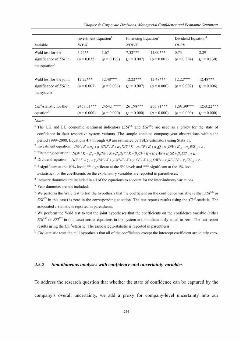
Chapter 4: Corporate Decisions, Managerial Confidence and Economic Sentiment
– 244 –
Variable Investment Equationb INV/K
Financing Equationc NDF/K
Dividend Equationd DIV/K
Wald test for the significance of ESI in the equationi
5.24** (p = 0.022)
1.67 (p = 0.197)
7.32*** (p = 0.007)
11.00*** (p = 0.001)
0.73 (p = 0.394)
2.29 (p = 0.130)
Wald test for the joint significance of ESI in the systemj
12.22*** (p = 0.007)
12.48*** (p = 0.006)
12.22*** (p = 0.007)
12.48*** (p = 0.006)
12.22*** (p = 0.007)
12.48*** (p = 0.006)
Chi2-statistic for the equationk
2458.31*** (p = 0.000)
2454.17*** (p = 0.000)
261.98*** (p = 0.000)
263.91*** (p = 0.000)
1291.99*** (p = 0.000)
1253.22*** (p = 0.000)
Notes: a. The UK and EU economic sentiment indicators (ESIUK and ESIEU) are used as a proxy for the state of
confidence in their respective system variants. The sample contains company-year observations within the period 1999–2008. Equations 4.7 through 4.9 are estimated by 3SLS estimators using Stata 11.
b. Investment equation: 161543210 ///// ESIKINVQKCFKDIVKNDFKINV . c. Financing equation: 16543210 //// ESISZTANKCFKDIVKINVKNDF . d. Dividend equation: 16543210 ///// ESITEREOWNKCFKNDFKINVKDIV . e. * significant at the 10% level; ** significant at the 5% level; and *** significant at the 1% level. f. z-statistics for the coefficients on the explanatory variables are reported in parentheses. g. Industry dummies are included in all of the equations to account for the inter-industry variations. h. Year dummies are not included. i. We perform the Wald test to test the hypothesis that the coefficient on the confidence variable (either ESIUK or
ESIEU in this case) is zero in the corresponding equation. The test reports results using the Chi2-statistic. The associated z-statistic is reported in parenthesis.
j. We perform the Wald test to test the joint hypotheses that the coefficients on the confidence variable (either ESIUK or ESIEU in this case) across equations in the system are simultaneously equal to zero. The test report results using the Chi2-statistic. The associated z-statistic is reported in parenthesis.
k. Chi2-statistic tests the null hypothesis that all of the coefficients except the intercept coefficient are jointly zero.
4.5.2 Simultaneous analyses with confidence and uncertainty variables
To address the research question that whether the state of confidence can be captured by the
company’s overall uncertainty, we add a proxy for company-level uncertainty into our
Chapter 4: Corporate Decisions, Managerial Confidence and Economic Sentiment
– 245 –
simultaneous equations system as another common exogenous determinant of corporate
decisions modelled in the system. Equations 4.10, 4.11 and 4.12 are estimated simultaneously
using the 3SLS estimators. The results are presented in Tables 4.8 and 4.9 where different
proxies for the state of confidence are used in their respective system variants. As is evident,
our findings with regard to the influences of managerial confidence and economic sentiment
on aspects of corporate behaviour persist even after controlling for company-level uncertainty
(UNC1). This clearly shows that managerial confidence and economic sentiment at aggregate
levels and the uncertainty at company level influence the corporate decisions of UK-listed
companies independently through different channels. More specifically, both the state of
aggregate confidence and the level of company idiosyncratic uncertainty have positive and
significant effects on corporate investment decisions. Debt financing decisions are heavily
influenced by the state of aggregate confidence but not by the level of company idiosyncratic
uncertainty, while dividend payout decisions are mainly affected by company idiosyncratic
uncertainty rather than the state of confidence at aggregate levels. The Wald test results report
in Tables 4.8 and 4.9 suggest that the state of confidence remain statistically significant even
in the presence of a proxy for overall uncertainty at company level.
According to our empirical results, corporate investment increases with both the state
of confidence at aggregate levels and the degree of uncertainty at company level. However,
managers of the UK-listed companies consider different financial choices in response to the
increased financing needs caused by different factors. If the increased investment spending is
Chapter 4: Corporate Decisions, Managerial Confidence and Economic Sentiment
– 246 –
due to high levels of managerial confidence or economic sentiment, companies tend to use
external debt financing more aggressively, but they are unlikely to cut dividends in response
to the increased financing needs. If the increased investment spending is caused by high levels
of company idiosyncratic uncertainty, companies tend to resort to internal funds by cutting
dividends rather than resorting to external funds by issuing new debts.
The different financial choices in response to the increased investment spending under
different situations might be interpreted as follows. When managerial confidence or economic
sentiment is high, managers are prone to attach higher probabilities to good outcomes, and
believe that their company is more profitable and less risky than it actually is. Therefore, they
are more confident of repaying debts in the future and maintaining dividend payout at desired
levels. Under this circumstance, managers are likely to resort to external debt financing to
finance the increased investment spending.
However, if the increased investment is due to high levels of uncertainty associated
with the company’s future prospects, managers are more cautious about possible future
financial distress if the outcomes turn out to be unfavourable. Accordingly, managers prefer to
retain the internally generated funds that otherwise would have been paid out to shareholders
as dividends to finance the increased investment spending under uncertainty. Debt financing is
used by managers with caution under uncertain circumstances, because higher levels of debt
are likely to exacerbate the degree of uncertainty and further increase the premium charged on
external funds.
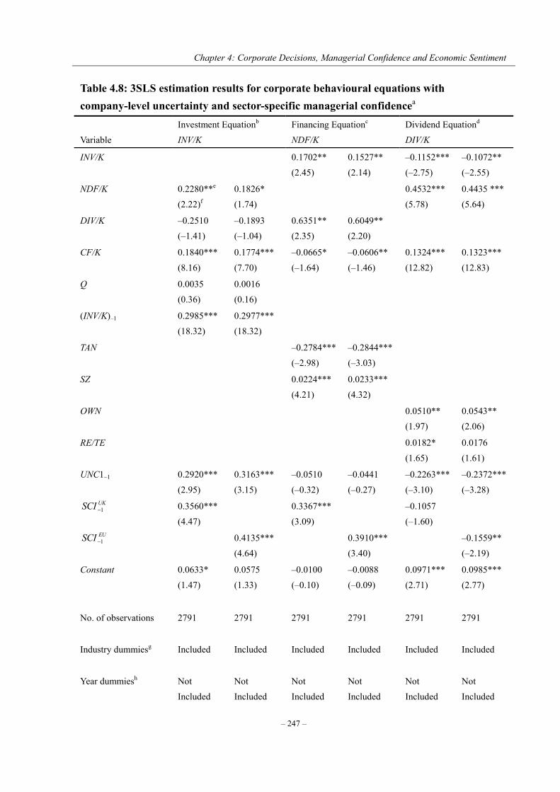
Chapter 4: Corporate Decisions, Managerial Confidence and Economic Sentiment
– 247 –
Table 4.8: 3SLS estimation results for corporate behavioural equations with company-level uncertainty and sector-specific managerial confidencea
Variable Investment Equationb INV/K
Financing Equationc NDF/K
Dividend Equationd DIV/K
INV/K 0.1702** (2.45)
0.1527** (2.14)
–0.1152*** (–2.75)
–0.1072** (–2.55)
NDF/K 0.2280**e (2.22)f
0.1826* (1.74)
0.4532*** (5.78)
0.4435 *** (5.64)
DIV/K –0.2510 (–1.41)
–0.1893 (–1.04)
0.6351** (2.35)
0.6049** (2.20)
CF/K 0.1840*** (8.16)
0.1774*** (7.70)
–0.0665* (–1.64)
–0.0606** (–1.46)
0.1324*** (12.82)
0.1323*** (12.83)
Q 0.0035 (0.36)
0.0016 (0.16)
(INV/K)–1 0.2985*** (18.32)
0.2977*** (18.32)
TAN –0.2784*** (–2.98)
–0.2844*** (–3.03)
SZ 0.0224*** (4.21)
0.0233*** (4.32)
OWN 0.0510** (1.97)
0.0543** (2.06)
RE/TE 0.0182* (1.65)
0.0176 (1.61)
UNC1–1 0.2920*** (2.95)
0.3163*** (3.15)
–0.0510 (–0.32)
–0.0441 (–0.27)
–0.2263*** (–3.10)
–0.2372*** (–3.28)
UKSCI 1 0.3560*** (4.47)
0.3367*** (3.09)
–0.1057 (–1.60)
EUSCI 1 0.4135*** (4.64)
0.3910*** (3.40)
–0.1559** (–2.19)
Constant 0.0633* (1.47)
0.0575 (1.33)
–0.0100 (–0.10)
–0.0088 (–0.09)
0.0971*** (2.71)
0.0985*** (2.77)
No. of observations
2791 2791 2791 2791 2791 2791
Industry dummiesg
Included Included Included Included Included Included
Year dummiesh Not Included
Not Included
Not Included
Not Included
Not Included
Not Included
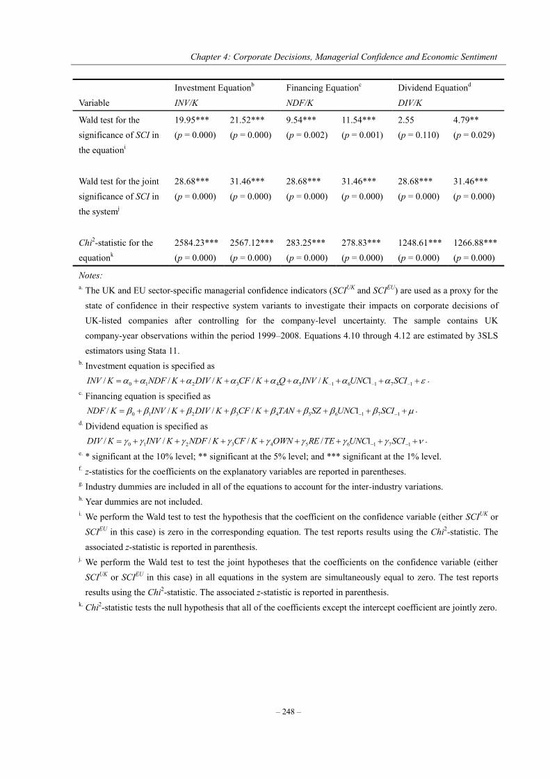
Chapter 4: Corporate Decisions, Managerial Confidence and Economic Sentiment
– 248 –
Variable Investment Equationb INV/K
Financing Equationc NDF/K
Dividend Equationd DIV/K
Wald test for the significance of SCI in the equationi
19.95*** (p = 0.000)
21.52*** (p = 0.000)
9.54*** (p = 0.002)
11.54*** (p = 0.001)
2.55 (p = 0.110)
4.79** (p = 0.029)
Wald test for the joint significance of SCI in the systemj
28.68*** (p = 0.000)
31.46*** (p = 0.000)
28.68*** (p = 0.000)
31.46*** (p = 0.000)
28.68*** (p = 0.000)
31.46*** (p = 0.000)
Chi2-statistic for the equationk
2584.23*** (p = 0.000)
2567.12*** (p = 0.000)
283.25*** (p = 0.000)
278.83*** (p = 0.000)
1248.61*** (p = 0.000)
1266.88*** (p = 0.000)
Notes: a. The UK and EU sector-specific managerial confidence indicators (SCIUK and SCIEU) are used as a proxy for the
state of confidence in their respective system variants to investigate their impacts on corporate decisions of UK-listed companies after controlling for the company-level uncertainty. The sample contains UK company-year observations within the period 1999–2008. Equations 4.10 through 4.12 are estimated by 3SLS estimators using Stata 11.
b. Investment equation is specified as 17161543210 1///// SCIUNCKINVQKCFKDIVKNDFKINV .
c. Financing equation is specified as 1716543210 1//// SCIUNCSZTANKCFKDIVKINVKNDF .
d. Dividend equation is specified as 1716543210 1///// SCIUNCTEREOWNKCFKNDFKINVKDIV .
e. * significant at the 10% level; ** significant at the 5% level; and *** significant at the 1% level. f. z-statistics for the coefficients on the explanatory variables are reported in parentheses. g. Industry dummies are included in all of the equations to account for the inter-industry variations. h. Year dummies are not included. i. We perform the Wald test to test the hypothesis that the coefficient on the confidence variable (either SCIUK or
SCIEU in this case) is zero in the corresponding equation. The test reports results using the Chi2-statistic. The associated z-statistic is reported in parenthesis.
j. We perform the Wald test to test the joint hypotheses that the coefficients on the confidence variable (either SCIUK or SCIEU in this case) in all equations in the system are simultaneously equal to zero. The test reports results using the Chi2-statistic. The associated z-statistic is reported in parenthesis.
k. Chi2-statistic tests the null hypothesis that all of the coefficients except the intercept coefficient are jointly zero.

Chapter 4: Corporate Decisions, Managerial Confidence and Economic Sentiment
– 249 –
Table 4.9: 3SLS estimation results for corporate behavioural equations with company-level uncertainty and economic sentimenta
Variable Investment Equationb INV/K
Financing Equationc NDF/K
Dividend Equationd DIV/K
INV/K 0.2010*** (3.05)
0.1946*** (2.94)
–0.1262*** (–3.09)
–0.1245*** (–3.02)
NDF/K 0.2674***e (2.62)f
0.2661*** (2.58)
0.4430*** (5.48)
0.4500 *** (5.48)
DIV/K –0.4438*** (–2.57)
–0.4328** (–2.51)
0.7219*** (2.83)
0.7142*** (2.78)
CF/K 0.2082*** (9.30)
0.2072*** (9.26)
–0.0832** (–2.16)
–0.0810** (–2.09)
0.1356*** (13.41)
0.1350*** (13.12)
Q 0.0086 (0.89)
0.0081 (0.84)
(INV/K)–1 0.2991*** (18.17)
0.2988*** (18.21)
TAN –0.0832*** (–2.16)
–0.2412*** (–2.78)
SZ 0.0222*** (4.19)
0.0218*** (4.12)
OWN 0.0431* (1.72)
0.0433* (1.72)
RE/TE 0.0172 (1.60)
0.0173 (1.59)
UNC1–1 0.2346** (2.36)
0.2516** (2.51)
–0.0057 (–0.04)
0.0307 (0.20)
–0.2276*** (–3.14)
–0.2441*** (–3.35)
UKESI 1 0.4192** (2.33)
0.5837** (2.55)
–0.1602 (–1.08)
EUESI 1 0.2369* (1.67)
0.5611*** (3.26)
–0.2338** (–2.01)
Constant –0.3543* (–1.44)
–0.1680 (–1.08)
–0.6537*** (–2.66)
–0.6336*** (–3.15)
0.2690* (1.76)
0.3478*** (2.86)
No. of observations
2791 2791 2791 2791 2791 2791
Industry dummiesg
Included Included Included Included Included Included
Year dummiesh Not Included
Not Included
Not Included
Not Included
Not Included
Not Included
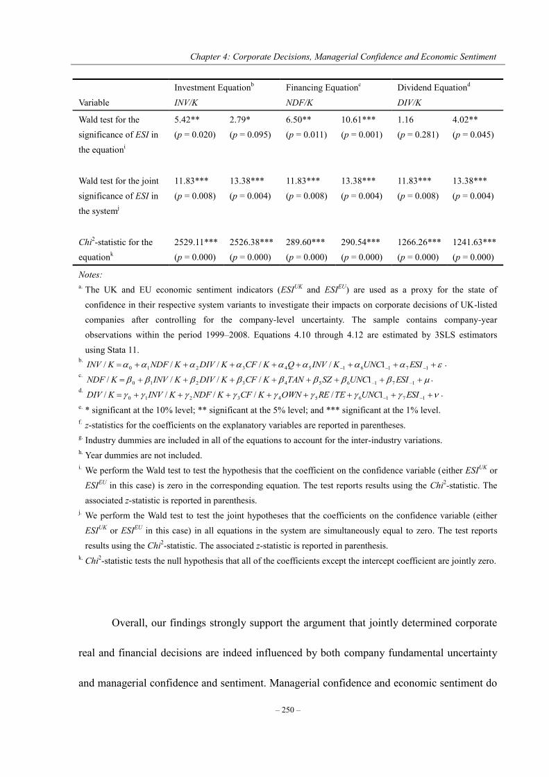
Chapter 4: Corporate Decisions, Managerial Confidence and Economic Sentiment
– 250 –
Variable Investment Equationb INV/K
Financing Equationc NDF/K
Dividend Equationd DIV/K
Wald test for the significance of ESI in the equationi
5.42** (p = 0.020)
2.79* (p = 0.095)
6.50** (p = 0.011)
10.61*** (p = 0.001)
1.16 (p = 0.281)
4.02** (p = 0.045)
Wald test for the joint significance of ESI in the systemj
11.83*** (p = 0.008)
13.38*** (p = 0.004)
11.83*** (p = 0.008)
13.38*** (p = 0.004)
11.83*** (p = 0.008)
13.38*** (p = 0.004)
Chi2-statistic for the equationk
2529.11*** (p = 0.000)
2526.38*** (p = 0.000)
289.60*** (p = 0.000)
290.54*** (p = 0.000)
1266.26*** (p = 0.000)
1241.63*** (p = 0.000)
Notes: a. The UK and EU economic sentiment indicators (ESIUK and ESIEU) are used as a proxy for the state of
confidence in their respective system variants to investigate their impacts on corporate decisions of UK-listed companies after controlling for the company-level uncertainty. The sample contains company-year observations within the period 1999–2008. Equations 4.10 through 4.12 are estimated by 3SLS estimators using Stata 11.
b. 17161543210 1///// ESIUNCKINVQKCFKDIVKNDFKINV . c. 1716543210 1//// ESIUNCSZTANKCFKDIVKINVKNDF . d. 1716543210 1///// ESIUNCTEREOWNKCFKNDFKINVKDIV . e. * significant at the 10% level; ** significant at the 5% level; and *** significant at the 1% level. f. z-statistics for the coefficients on the explanatory variables are reported in parentheses. g. Industry dummies are included in all of the equations to account for the inter-industry variations. h. Year dummies are not included. i. We perform the Wald test to test the hypothesis that the coefficient on the confidence variable (either ESIUK or
ESIEU in this case) is zero in the corresponding equation. The test reports results using the Chi2-statistic. The associated z-statistic is reported in parenthesis.
j. We perform the Wald test to test the joint hypotheses that the coefficients on the confidence variable (either ESIUK or ESIEU in this case) in all equations in the system are simultaneously equal to zero. The test reports results using the Chi2-statistic. The associated z-statistic is reported in parenthesis.
k. Chi2-statistic tests the null hypothesis that all of the coefficients except the intercept coefficient are jointly zero.
Overall, our findings strongly support the argument that jointly determined corporate
real and financial decisions are indeed influenced by both company fundamental uncertainty
and managerial confidence and sentiment. Managerial confidence and economic sentiment do

Chapter 4: Corporate Decisions, Managerial Confidence and Economic Sentiment
– 251 –
provide additional information in explaining aspects of corporate behaviour over the
fundamental factors, as indicated by the statistically significant Wald test results across all of
the simultaneous equations system variants.
4.6 Robustness tests and further evidence
4.6.1 Robustness tests and results
To gauge the sensitivity of using the arithmetic average of monthly values over each year as
proxies for managerial confidence and economic sentiment, we also follow Oliver and
Mefteh’s (2010) methodology by considering the December figures (SCIUKDEC, SCIEUDEC,
ESIUKDEC and ESIEUDEC) as the relevant measures of managerial confidence and economic
sentiment and re-estimating our simultaneous equations system. As can be seen from
Appendices 4.C and 4.D, the results replicated using the December figures are largely
consistent with those reported in Section 4.5 in terms of the signs and significance levels of
the estimated coefficients in all of the corporate behavioural equations, except that the state of
managerial confidence and economic sentiment in December is likely to have a more
significant negative influence on corporate payout decisions than the arithmetic average
values of managerial confidence and economic sentiment indicators over the year.
In addition, we also calculate series with the percentage changes in the economic
sentiment indicators as alternative proxies for the state of confidence to re-estimate our
systems. The 3SLS estimation results are reported in Appendices 4.E. Compared with the

Chapter 4: Corporate Decisions, Managerial Confidence and Economic Sentiment
– 252 –
economic sentiment indicators in levels (see Table 4.7), the percentage changes in the
economic sentiment indicators ( EUESI 1 ) have lower explanatory powers in both the debt
financing and dividend payout equations, suggesting that corporate financial decisions are
more likely to be influence by the level of economic sentiment rather than the changes in it.
We do not attempt to calculate series with the percentage changes in the managerial
confidence indicators. Unlike the economic sentiment indicators which are scaled to have a
long-run mean of 100%, the value of managerial confidence indicators are close to zero with
both positive and negative values. The percentage changes in such time series, thus, are likely
to be extremely noisy and carry little information about changes in managerial confidence.
Furthermore, given the fact that 3SLS estimators are more likely to be vulnerable to
specification errors as compared to the limited information methods, we also apply the 2SLS
estimation to the simultaneous equations system variants as robustness check. The 2SLS
estimation results are presented in Appendices 4.F and 4.G. The influences of the state of
managerial confidence and economic sentiment indicated in the 2SLS estimation results seem
to be more pronounced compared with those suggested by 3SLS estimation results reported in
Tables 4.6 and 4.7. However, the simultaneity among the corporate decisions seems to be
relatively weak when the 2SLS estimations are applied.
Overall, we conclude that our results for the relations between corporate decisions and
the state of managerial confidence and economic sentiment are robust to different model
specifications, variable measurements and estimation methods.
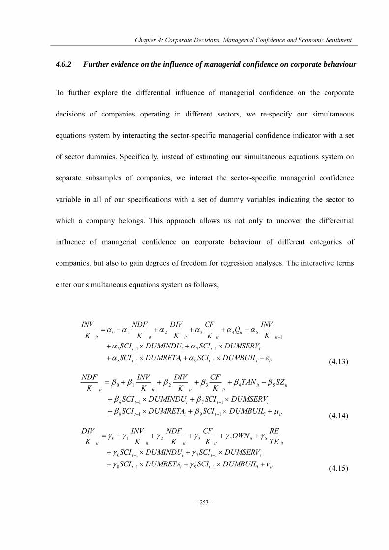
Chapter 4: Corporate Decisions, Managerial Confidence and Economic Sentiment
– 253 –
4.6.2 Further evidence on the influence of managerial confidence on corporate behaviour
To further explore the differential influence of managerial confidence on the corporate
decisions of companies operating in different sectors, we re-specify our simultaneous
equations system by interacting the sector-specific managerial confidence indicator with a set
of sector dummies. Specifically, instead of estimating our simultaneous equations system on
separate subsamples of companies, we interact the sector-specific managerial confidence
variable in all of our specifications with a set of dummy variables indicating the sector to
which a company belongs. This approach allows us not only to uncover the differential
influence of managerial confidence on corporate behaviour of different categories of
companies, but also to gain degrees of freedom for regression analyses. The interactive terms
enter our simultaneous equations system as follows,
ititit
itit
itit
itititit
DUMBUILSCIDUMRETASCIDUMSERVSCIDUMINDUSCI
KINVQ
KCF
KDIV
KNDF
KINV
1918
1716
1543210
(4.13)
ititit
itit
itititititit
DUMBUILSCIDUMRETASCIDUMSERVSCIDUMINDUSCI
SZTANK
CFK
DIVK
INVK
NDF
1918
1716
543210
(4.14)
ititit
itit
itit
itititit
DUMBUILSCIDUMRETASCIDUMSERVSCIDUMINDUSCI
TEREOWN
KCF
KNDF
KINV
KDIV
1918
1716
543210
(4.15)

Chapter 4: Corporate Decisions, Managerial Confidence and Economic Sentiment
– 254 –
where DUMINDU, DUMSERV, DUMRETA and DUMBUIL are the sector dummy variables
represent manufacturing, services, retail trade and construction sectors, respectively. A sector
dummy variable is set equal to 1 for companies operating in the sector; and 0, otherwise. The
estimated coefficients for the interactive terms are expected to show the differences in the
influence of managerial confidence on corporate decisions across the four sectors. In addition,
we also augment the simultaneities equation system with interactive terms by including the
proxy for company-level uncertainty (UNC1) as follows,
ititit
itit
itit
ititititit
DUMBUILSCIDUMRETASCIDUMSERVSCIDUMINDUSCI
UNCK
INVQK
CFK
DIVK
NDFK
INV
11019
1817
161
543210
1
(4.16)
ititit
itit
ititititititit
DUMBUILSCIDUMRETASCIDUMSERVSCIDUMINDUSCI
UNCSZTANK
CFK
DIVK
INVK
NDF
11019
1817
16543210
1
(4.17)
ititit
itit
itit
ititititit
DUMBUILSCIDUMRETASCIDUMSERVSCIDUMINDUSCI
UNCTEREOWN
KCF
KNDF
KINV
KDIV
11019
1817
16543210
1
(4.18)
Chapter 4: Corporate Decisions, Managerial Confidence and Economic Sentiment
– 255 –
Table 4.10 reports the estimation results for the system variants which are comprised
of Equations 4.13–4.15. The results for the endogenous variables and the other control
variables are similar to those reported in Section 4.5. Moreover, the results reported in Table
4.10 reveal more detailed evidence on how managerial confidence influences corporate
decisions of companies in different sectors.
Specifically, the corporate investment decisions in all sectors are positively correlated
with the shifts in sectoral managerial confidence. The positive effect of managerial confidence
on corporate investment spending is particularly profound for the construction sector, as
indicated by the large and highly significant coefficient estimated for the interactive terms for
the construction sector. However, the influence of managerial confidence on manufacturing
companies’ investment behaviour is rather weak and not significant at the usual significance
levels. As for debt financing decisions, services and manufacturing companies are likely to
borrow more aggressively when the sectoral sentiment is high, while retail trade and
construction companies’ financing decisions are not evidently influenced by the level of
managerial confidence and sentiment. Although the effect of managerial confidence on
dividend payout policies of UK-listed companies is insignificant as a whole, the coefficients
on the interactive terms reported in Table 4.10 indicate that companies in the services sector
tend to retain more internally generated cash flow by cutting dividend payouts to finance their
increased financing needs when their managers are confident about future company
performance.
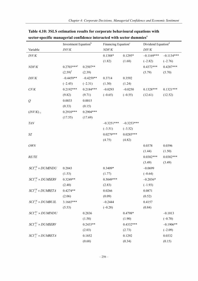
Chapter 4: Corporate Decisions, Managerial Confidence and Economic Sentiment
– 256 –
Table 4.10: 3SLS estimation results for corporate behavioural equations with sector-specific managerial confidence interacted with sector dummiesa
Variable Investment Equationb INV/K
Financing Equationc NDF/K
Dividend Equationd DIV/K
INV/K 0.1388* (1.82)
0.1295* (1.68)
–0.1169*** (–2.82)
–0.1134*** (–2.76)
NDF/K 0.2703***e (2.59)f
0.2507** (2.39)
0.4372*** (5.79)
0.4287*** (5.70)
DIV/K –0.4459** (–2.45)
–0.4259** (–2.31)
0.3714 (1.30)
0.3592 (1.24)
CF/K 0.2192*** (9.82)
0.2184*** (9.71)
–0.0293 (–0.65)
–0.0250 (–0.55)
0.1328*** (12.61)
0.1321*** (12.52)
Q 0.0033 (0.33)
0.0015 (0.15)
(INV/K)–1 0.2910*** (17.55)
0.2904*** (17.69)
TAN –0.3251*** (–3.51)
–0.3253*** (–3.52)
SZ 0.0279*** (4.75)
0.0285*** (4.82)
OWN 0.0378 (1.44)
0.0396 (1.50)
RE/TE 0.0382*** (3.49)
0.0382*** (3.49)
DUMINDUSCI UK 1 0.2043 (1.53)
0.3409* (1.77)
–0.0699 (–0.64)
DUMSERVSCI UK 1 0.3249** (2.40)
0.5049*** (2.83)
–0.2036* (–1.93)
DUMRETASCI UK 1 0.4274** (2.06)
0.0266 (0.09)
0.0871 (0.52)
DUMBUILSCI UK 1 3.1665*** (5.53)
–0.2444 (–0.28)
0.4157 (0.84)
DUMINDUSCI EU 1 0.2836 (1.58)
0.4798* (1.90)
–0.1013 (–0.70)
DUMSERVSCI EU 1 0.2433** (2.03)
0.4332*** (2.73)
–0.1906** (–2.09)
DUMRETASCI EU 1
0.1852 (0.68)
0.1292 (0.34)
0.0332 (0.15)
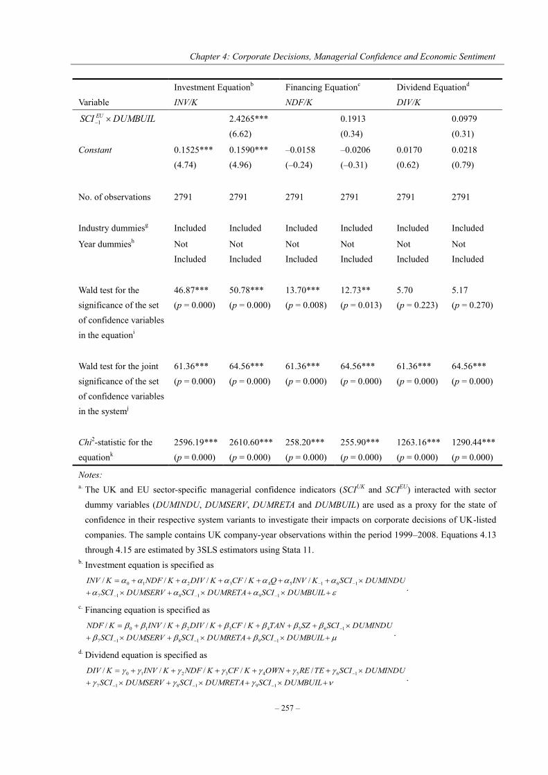
Chapter 4: Corporate Decisions, Managerial Confidence and Economic Sentiment
– 257 –
Variable Investment Equationb INV/K
Financing Equationc NDF/K
Dividend Equationd DIV/K
DUMBUILSCI EU 1 2.4265*** (6.62)
0.1913 (0.34)
0.0979 (0.31)
Constant 0.1525*** (4.74)
0.1590*** (4.96)
–0.0158 (–0.24)
–0.0206 (–0.31)
0.0170 (0.62)
0.0218 (0.79)
No. of observations
2791 2791 2791 2791 2791 2791
Industry dummiesg Included Included Included Included Included Included
Year dummiesh
Not Included
Not Included
Not Included
Not Included
Not Included
Not Included
Wald test for the significance of the set of confidence variables in the equationi
46.87*** (p = 0.000)
50.78*** (p = 0.000)
13.70*** (p = 0.008)
12.73** (p = 0.013)
5.70 (p = 0.223)
5.17 (p = 0.270)
Wald test for the joint significance of the set of confidence variables in the systemj
61.36*** (p = 0.000)
64.56*** (p = 0.000)
61.36*** (p = 0.000)
64.56*** (p = 0.000)
61.36*** (p = 0.000)
64.56*** (p = 0.000)
Chi2-statistic for the equationk
2596.19*** (p = 0.000)
2610.60*** (p = 0.000)
258.20*** (p = 0.000)
255.90*** (p = 0.000)
1263.16*** (p = 0.000)
1290.44*** (p = 0.000)
Notes: a. The UK and EU sector-specific managerial confidence indicators (SCIUK and SCIEU) interacted with sector
dummy variables (DUMINDU, DUMSERV, DUMRETA and DUMBUIL) are used as a proxy for the state of confidence in their respective system variants to investigate their impacts on corporate decisions of UK-listed companies. The sample contains UK company-year observations within the period 1999–2008. Equations 4.13 through 4.15 are estimated by 3SLS estimators using Stata 11.
b. Investment equation is specified as
DUMBUILSCIDUMRETASCIDUMSERVSCIDUMINDUSCIKINVQKCFKDIVKNDFKINV
191817
161543210 /////.
c. Financing equation is specified as
DUMBUILSCIDUMRETASCIDUMSERVSCIDUMINDUSCISZTANKCFKDIVKINVKNDF
191817
16543210 ////.
d. Dividend equation is specified as
DUMBUILSCIDUMRETASCIDUMSERVSCIDUMINDUSCITEREOWNKCFKNDFKINVKDIV
191817
16543210 /////.

Chapter 4: Corporate Decisions, Managerial Confidence and Economic Sentiment
– 258 –
e. * significant at the 10% level; ** significant at the 5% level; and *** significant at the 1% level. f. z-statistics are reported in parentheses. g. Industry dummies are included in all of the equations to account for the inter-industry variations. h. Year dummies are not included. i. We perform the Wald test to test the hypothesis that the coefficients on the set of interaction terms are zero in
the corresponding equation. The test reports results using the Chi2-statistic. The associated z-statistic is reported in parenthesis.
j. We perform the Wald test to test the joint hypotheses that the coefficients on the interaction terms in all equations in the system are simultaneously equal to zero. The test reports results using the Chi2-statistic. The associated z-statistic is reported in parenthesis.
k. Chi2-statistic tests the null hypothesis that all of the coefficients except the intercept coefficient are jointly zero.
Taken together, it seems that company in the services sector act more aggressively
when their managers are confident. Specifically, they tend to invest in capital stock more
intensively, use debt financing more heavily and cut dividends more decisively when the
sectoral sentiment is high. There are a number of possible explanations for these results found
for the services sector. One reason for these results might be the basic characteristic of the
companies in this sector. Unlike companies in the other sectors, companies in services sector
offer the production of services using their knowledge and time. They typically do not have a
large stock of capital goods and finished products, which leads naturally to a relatively low
level of asset tangibility. Given the lack of pledgeable assets, companies in service sector are
more likely to be externally financially constrained, and therefore they might be forced not
only to resort to external funds by issuing new debt but also to resort to internal funds by
cutting dividends, in an attempt to finance increased investments when the sectoral sentiment
is high.
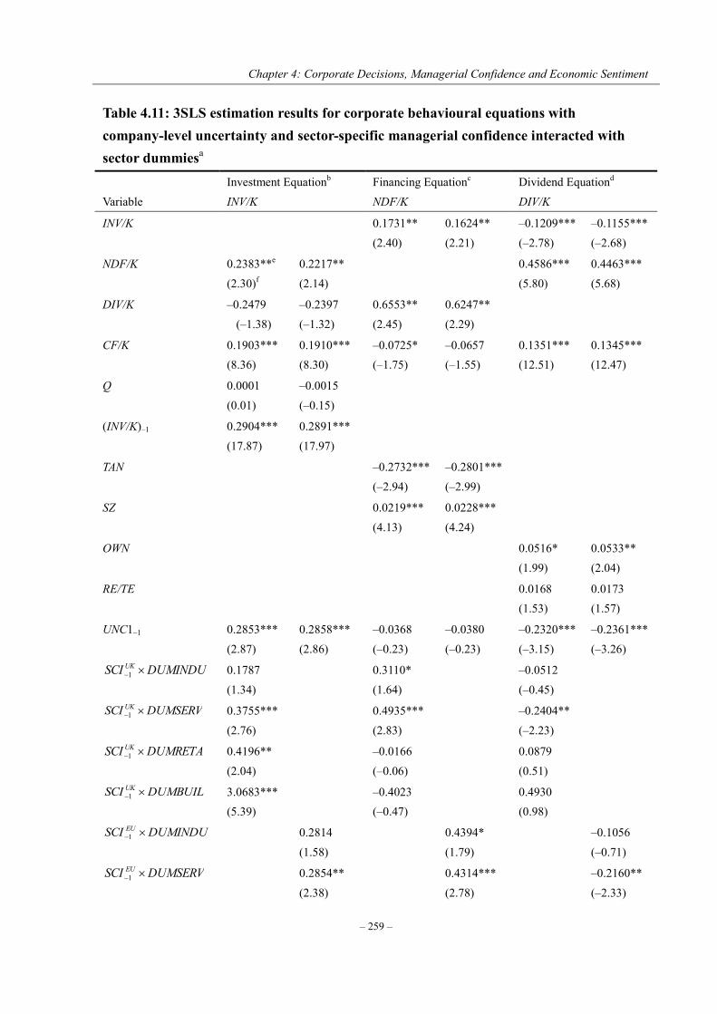
Chapter 4: Corporate Decisions, Managerial Confidence and Economic Sentiment
– 259 –
Table 4.11: 3SLS estimation results for corporate behavioural equations with company-level uncertainty and sector-specific managerial confidence interacted with sector dummiesa
Variable Investment Equationb INV/K
Financing Equationc NDF/K
Dividend Equationd DIV/K
INV/K 0.1731** (2.40)
0.1624** (2.21)
–0.1209*** (–2.78)
–0.1155*** (–2.68)
NDF/K 0.2383**e (2.30)f
0.2217** (2.14)
0.4586*** (5.80)
0.4463*** (5.68)
DIV/K –0.2479 (–1.38)
–0.2397 (–1.32)
0.6553** (2.45)
0.6247** (2.29)
CF/K 0.1903*** (8.36)
0.1910*** (8.30)
–0.0725* (–1.75)
–0.0657 (–1.55)
0.1351*** (12.51)
0.1345*** (12.47)
Q 0.0001 (0.01)
–0.0015 (–0.15)
(INV/K)–1 0.2904*** (17.87)
0.2891*** (17.97)
TAN –0.2732*** (–2.94)
–0.2801*** (–2.99)
SZ 0.0219*** (4.13)
0.0228*** (4.24)
OWN 0.0516* (1.99)
0.0533** (2.04)
RE/TE 0.0168 (1.53)
0.0173 (1.57)
UNC1–1 0.2853*** (2.87)
0.2858*** (2.86)
–0.0368 (–0.23)
–0.0380 (–0.23)
–0.2320*** (–3.15)
–0.2361*** (–3.26)
DUMINDUSCI UK 1 0.1787 (1.34)
0.3110* (1.64)
–0.0512 (–0.45)
DUMSERVSCI UK 1 0.3755*** (2.76)
0.4935*** (2.83)
–0.2404** (–2.23)
DUMRETASCI UK 1 0.4196** (2.04)
–0.0166 (–0.06)
0.0879 (0.51)
DUMBUILSCI UK 1 3.0683*** (5.39)
–0.4023 (–0.47)
0.4930 (0.98)
DUMINDUSCI EU 1 0.2814 (1.58)
0.4394* (1.79)
–0.1056 (–0.71)
DUMSERVSCI EU 1
0.2854** (2.38)
0.4314*** (2.78)
–0.2160** (–2.33)
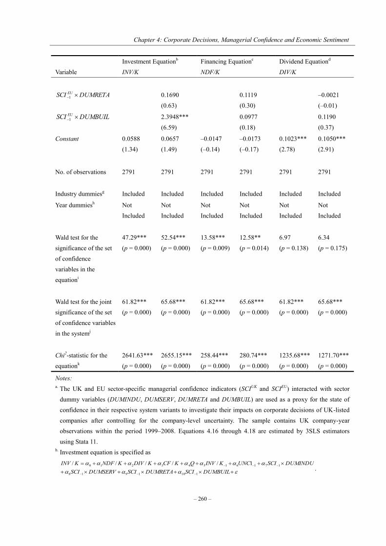
Chapter 4: Corporate Decisions, Managerial Confidence and Economic Sentiment
– 260 –
Variable Investment Equationb INV/K
Financing Equationc NDF/K
Dividend Equationd DIV/K
DUMRETASCI EU 1 0.1690 (0.63)
0.1119 (0.30)
–0.0021 (–0.01)
DUMBUILSCI EU 1 2.3948*** (6.59)
0.0977 (0.18)
0.1190 (0.37)
Constant 0.0588 (1.34)
0.0657 (1.49)
–0.0147 (–0.14)
–0.0173 (–0.17)
0.1023*** (2.78)
0.1050*** (2.91)
No. of observations
2791 2791 2791 2791 2791 2791
Industry dummiesg Included Included Included Included Included Included
Year dummiesh
Not Included
Not Included
Not Included
Not Included
Not Included
Not Included
Wald test for the significance of the set of confidence variables in the equationi
47.29*** (p = 0.000)
52.54*** (p = 0.000)
13.58*** (p = 0.009)
12.58** (p = 0.014)
6.97 (p = 0.138)
6.34 (p = 0.175)
Wald test for the joint significance of the set of confidence variables in the systemj
61.82*** (p = 0.000)
65.68*** (p = 0.000)
61.82*** (p = 0.000)
65.68*** (p = 0.000)
61.82*** (p = 0.000)
65.68*** (p = 0.000)
Chi2-statistic for the equationk
2641.63*** (p = 0.000)
2655.15*** (p = 0.000)
258.44*** (p = 0.000)
280.74*** (p = 0.000)
1235.68*** (p = 0.000)
1271.70*** (p = 0.000)
Notes: a. The UK and EU sector-specific managerial confidence indicators (SCIUK and SCIEU) interacted with sector
dummy variables (DUMINDU, DUMSERV, DUMRETA and DUMBUIL) are used as a proxy for the state of confidence in their respective system variants to investigate their impacts on corporate decisions of UK-listed companies after controlling for the company-level uncertainty. The sample contains UK company-year observations within the period 1999–2008. Equations 4.16 through 4.18 are estimated by 3SLS estimators using Stata 11.
b. Investment equation is specified as
DUMBUILSCIDUMRETASCIDUMSERVSCIDUMINDUSCIUNCKINVQKCFKDIVKNDFKINV
1101918
17161543210 1/////.
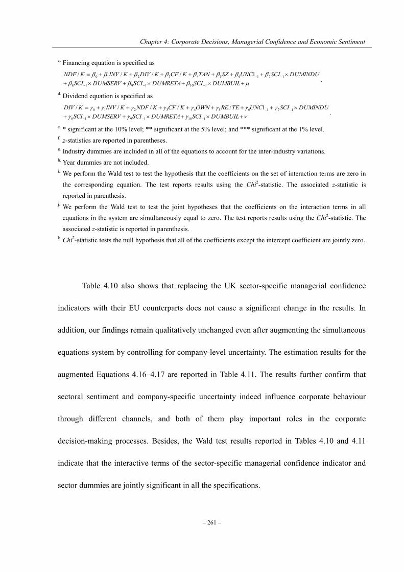
Chapter 4: Corporate Decisions, Managerial Confidence and Economic Sentiment
– 261 –
c. Financing equation is specified as
DUMBUILSCIDUMRETASCIDUMSERVSCIDUMINDUSCIUNCSZTANKCFKDIVKINVKNDF
1101918
1716543210 1////.
d. Dividend equation is specified as
DUMBUILSCIDUMRETASCIDUMSERVSCIDUMINDUSCIUNCTEREOWNKCFKNDFKINVKDIV
1101918
1716543210 1/////.
e. * significant at the 10% level; ** significant at the 5% level; and *** significant at the 1% level. f. z-statistics are reported in parentheses. g. Industry dummies are included in all of the equations to account for the inter-industry variations. h. Year dummies are not included. i. We perform the Wald test to test the hypothesis that the coefficients on the set of interaction terms are zero in
the corresponding equation. The test reports results using the Chi2-statistic. The associated z-statistic is reported in parenthesis.
j. We perform the Wald test to test the joint hypotheses that the coefficients on the interaction terms in all equations in the system are simultaneously equal to zero. The test reports results using the Chi2-statistic. The associated z-statistic is reported in parenthesis.
k. Chi2-statistic tests the null hypothesis that all of the coefficients except the intercept coefficient are jointly zero.
Table 4.10 also shows that replacing the UK sector-specific managerial confidence
indicators with their EU counterparts does not cause a significant change in the results. In
addition, our findings remain qualitatively unchanged even after augmenting the simultaneous
equations system by controlling for company-level uncertainty. The estimation results for the
augmented Equations 4.16–4.17 are reported in Table 4.11. The results further confirm that
sectoral sentiment and company-specific uncertainty indeed influence corporate behaviour
through different channels, and both of them play important roles in the corporate
decision-making processes. Besides, the Wald test results reported in Tables 4.10 and 4.11
indicate that the interactive terms of the sector-specific managerial confidence indicator and
sector dummies are jointly significant in all the specifications.
Chapter 4: Corporate Decisions, Managerial Confidence and Economic Sentiment
– 262 –
4.7 Concluding remarks
In this chapter, we offer the first systematic attempt to investigate the impacts of managerial
confidence and economic sentiment at aggregate levels on jointly determined corporate
investment, financing and payout decisions, using a large panel of UK-listed companies
observed within the period from 1999 to 2008. The relations between corporate decisions and
the state of sentiment and confidence are examined within a simultaneous equations system
which allows for contemporaneous interdependence among the corporate decisions. Our
empirical results confirm the joint determination of these corporate decisions, as implied by
the flow-of-funds framework. More importantly, we find that the state of confidence at
aggregate levels, as proxied by the UK or EU sector-specific managerial confidence indicators
or economic sentiment indicators, has significantly positive effects on companies’ real
investment and debt financing decisions. The positive effects remain statistically significant
even after controlling for company-specific uncertainty and other fundamental variables.
This chapter, therefore, provides empirical evidence shows that managerial
psychological bias does indeed play an important role in the determination of corporate
decisions, contributing to the small but growing literature on behavioural corporate finance. In
addition, our results also provide empirical evidence that managers’ psychological bias and
companies’ fundamental uncertainty influence corporate decisions independently through
different channels. Both managerial confidence and fundamental uncertainty have a positive
real effect on corporate investment decisions. However, managers consider different financial

Chapter 4: Corporate Decisions, Managerial Confidence and Economic Sentiment
– 263 –
choices in response to the increased financing needs caused by different factors. To finance
the increased investment spending caused by high managerial confidence and economic
sentiment, companies tend to use external debt financing rather than cutting dividends paid to
their shareholders. To finance the increased investment spending under high levels of
uncertainty, companies prefer to resort to internal finance by cutting dividends rather than
resorting to external finance by issuing new debts.
Besides, we find that companies in the services sector tend to behave more
aggressively when their managers are confident, which might be attributable to the lack of
pledgeable assets. Specifically, they invest in capital stock more intensively, use debt
financing more heavily, and cut dividends more decisively when the sectoral sentiment is
high.
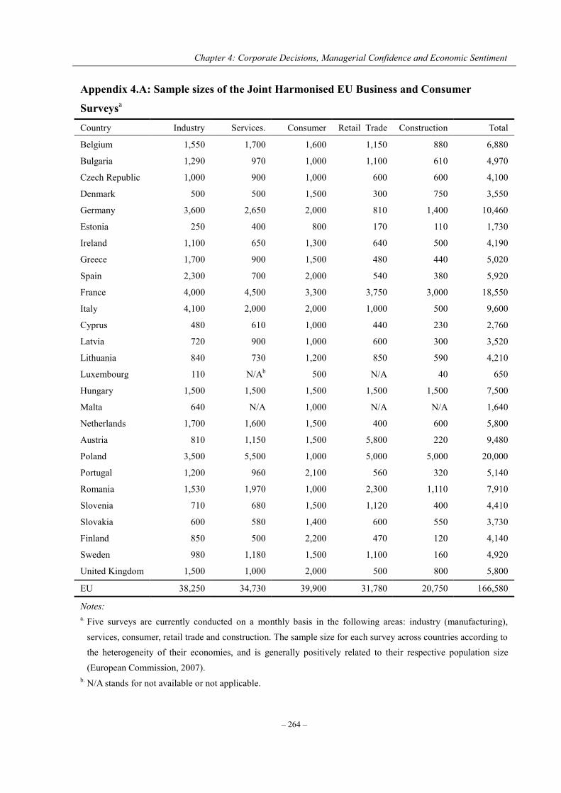
Chapter 4: Corporate Decisions, Managerial Confidence and Economic Sentiment
– 264 –
Appendix 4.A: Sample sizes of the Joint Harmonised EU Business and Consumer
Surveysa
Country Industry Services. Consumer Retail Trade Construction Total
Belgium 1,550 1,700 1,600 1,150 880 6,880
Bulgaria 1,290 970 1,000 1,100 610 4,970
Czech Republic 1,000 900 1,000 600 600 4,100
Denmark 500 500 1,500 300 750 3,550
Germany 3,600 2,650 2,000 810 1,400 10,460
Estonia 250 400 800 170 110 1,730
Ireland 1,100 650 1,300 640 500 4,190
Greece 1,700 900 1,500 480 440 5,020
Spain 2,300 700 2,000 540 380 5,920
France 4,000 4,500 3,300 3,750 3,000 18,550
Italy 4,100 2,000 2,000 1,000 500 9,600
Cyprus 480 610 1,000 440 230 2,760
Latvia 720 900 1,000 600 300 3,520
Lithuania 840 730 1,200 850 590 4,210
Luxembourg 110 N/Ab 500 N/A 40 650
Hungary 1,500 1,500 1,500 1,500 1,500 7,500
Malta 640 N/A 1,000 N/A N/A 1,640
Netherlands 1,700 1,600 1,500 400 600 5,800
Austria 810 1,150 1,500 5,800 220 9,480
Poland 3,500 5,500 1,000 5,000 5,000 20,000
Portugal 1,200 960 2,100 560 320 5,140
Romania 1,530 1,970 1,000 2,300 1,110 7,910
Slovenia 710 680 1,500 1,120 400 4,410
Slovakia 600 580 1,400 600 550 3,730
Finland 850 500 2,200 470 120 4,140
Sweden 980 1,180 1,500 1,100 160 4,920
United Kingdom 1,500 1,000 2,000 500 800 5,800
EU 38,250 34,730 39,900 31,780 20,750 166,580
Notes: a. Five surveys are currently conducted on a monthly basis in the following areas: industry (manufacturing),
services, consumer, retail trade and construction. The sample size for each survey across countries according to the heterogeneity of their economies, and is generally positively related to their respective population size (European Commission, 2007).
b. N/A stands for not available or not applicable.

Chapter 4: Corporate Decisions, Managerial Confidence and Economic Sentiment
– 265 –
Appendix 4.B: EU Programme of Business and Consumer Surveys
Panel A: The Joint Harmonised EU Industry Survey Questionnaire
Q1 How has your production developed over the past 3 months? It has…
+ increased = remained unchanged
– decreased Q2 Do you consider your current overall order books to be…?*a + more than sufficient (above normal) = sufficient (normal for the season)
– not sufficient (below normal) Q3 Do you consider your current export order books to be…? + more than sufficient (above normal) = sufficient (normal for the season)
– not sufficient (below normal) Q4 Do you consider your current stock of finished products to be…?*b + too large (above normal) = adequate (normal for the season)
– too small (below normal) Q5 How do you expect your production to develop over the next 3 months?
It will…* + increase = remain unchanged
– decrease Q6 How do you expect your selling prices to change over the next 3 months?
They will… + increase = remain unchanged
– decrease Q7 How do you expect your firm’s total employment to change over the next 3 months?
It will… + increase = remain unchanged
– decrease

Chapter 4: Corporate Decisions, Managerial Confidence and Economic Sentiment
– 266 –
Panel B: The Joint Harmonised EU Services Survey Questionnaire
Q1 How has your business situation developed over the past 3 months? It has…*
+ increased = remained unchanged
– decreased Q2 How has demand (turnover) for your company’s services changed over the past 3months?
It has…* + increased = remained unchanged
– decreased Q3 How do you expect the demand (turnover) for your company’s services to change over the next 3 months?
It will…* + increase = remain unchanged
– decrease Q4 How has your firm’s total employment changed over the past 3 months?
It has… + increased = remained unchanged
– decreased Q5 How do you expect your firm’s total employment to change over the next 3 months?
It will… + increase = remain unchanged
– decrease Q6 How do you expect the prices you charge to change over the next 3 months?
They will… + increase = remain unchanged
– decrease

Chapter 4: Corporate Decisions, Managerial Confidence and Economic Sentiment
– 267 –
Panel C: The Joint Harmonised EU Retail Trade Survey Questionnaire
Q1 How has (have) your business activity (sales) developed over the past 3 months? It has (They have)…*
+ improved (increased) = remained unchanged – deteriorated (decreased) Q2 Do you consider the volume of stock you currently hold to be…?*c + too large (above normal) = adequate (normal for the season) – too small (below normal) Q3 How do you expect your orders placed with suppliers to change over the next 3 months?
They will… + increase = remain unchanged – decrease Q4 How do you expect your business activity (sales) to change over the next 3 months?
It (They) will…* + improve (increase) = remain unchanged – deteriorate (decrease) Q5 How do you expect your firm’s total employment to change over the next 3 months?
It will… + increase = remain unchanged – decrease Q6 How do you expect the prices you charge to change over the next 3 months?
They will… + increase = remain unchanged – decrease

Chapter 4: Corporate Decisions, Managerial Confidence and Economic Sentiment
– 268 –
Panel D: The Joint Harmonised EU Construction Survey Questionnaire
Q1 How has your building activity developed over the past 3 months? It has…
+ increased = remained unchanged – decreased Q2 What main factors are currently limiting your building activity? · none · insufficient demand · weather conditions · shortage of labour force · shortage of material and/or equipment · financial constraints · other factors Q3 Do you consider your current overall order books to be…?* + more than sufficient (above normal) = sufficient (normal for the season) – not sufficient (below normal) Q4 How do you expect your firm’s total employment to change over the next 3 months?
It will…* + increase = remain unchanged – decrease Q5 How do you expect the prices you charge to change over the next 3 months?
They will… + increase = remain unchanged – decrease

Chapter 4: Corporate Decisions, Managerial Confidence and Economic Sentiment
– 269 –
Panel E: The Joint Harmonised EU Consumer Survey Questionnaire
Q1 How has the financial situation of your household changed over the last 12 months? It has…
+ + got a lot better + got a little better = stayed the same – got a little worse – – got a lot worse
N don’t know Q2 How do you expect the financial position of your household to change over the next 12 months?
It will…* + + get a lot better + get a little better = stay the same – get a little worse – – get a lot worse N don’t know Q3 How do you think the general economic situation in the country has changed over the past 12 months?
It has… + + got a lot better + got a little better = stayed the same – got a little worse – – got a lot worse N don’t know Q4 How do you expect the general economic situation in this country to develop over the next 12 months?
It will…* + + get a lot better + get a little better = stay the same – get a little worse – – get a lot worse N don’t know

Chapter 4: Corporate Decisions, Managerial Confidence and Economic Sentiment
– 270 –
Q5 How do you think that consumer prices have developed over the last 12 months? They have…
+ + risen a lot + risen moderately = risen slightly – stayed about the same – – fallen N don’t know Q7 How do you expect the number of people unemployed in this country to change over the next 12 months?
The number will…*d + + increase sharply + increase slightly = remain the same – fall slightly – – fall sharply N don’t know Q8 In view of the general economic situation, do you think that now it is the right moment for people to make
major purchases such as furniture, electrical/electronic devices, etc.? + + yes, it is the right moment now = it is neither the right moment nor the wrong moment – – no, it is not the right moment now N don’t know Q9 Compared to the past 12 months, do you expect to spend more or less money on major purchases (furniture,
electrical/electronic devices, etc.) over the next 12 months? I will spend…
+ + much more + a little more = about the same – a little less – – much less N don’t know Q10 In view of the general economic situation, do you think that now is…? + + a very good moment to save + a fairly good moment to save – not a good moment to save – – a very bad moment to save N don’t know

Chapter 4: Corporate Decisions, Managerial Confidence and Economic Sentiment
– 271 –
Q11 Over the next 12 months, how likely is it that you save any money?* + + very likely + fairly likely – not likely – – not at all likely N don’t know Q12 Which of these statement best describes the current financial situation of your household? + + we are saving a lot + we are saving a little = we are just managing to make ends meet on our income – we are having to draw on our savings – – we are running into debt N don’t know Notes: a. * indicates questions chosen from the full set of questions in each individual survey to construct the
corresponding sector-specific confidence indicator and the economic sentiment indicator. b. The balance value of Q4 in Panel A is used to construct the managerial confidence indicator for manufacturing
sector with an inverted sign. c. The balance value of Q2 in Panel C is used to construct the managerial confidence indicator for retail trade
sector with an inverted sign. d. The balance value of Q7 in Panel E is used to construct the consumer confidence indicator with an inverted
sign
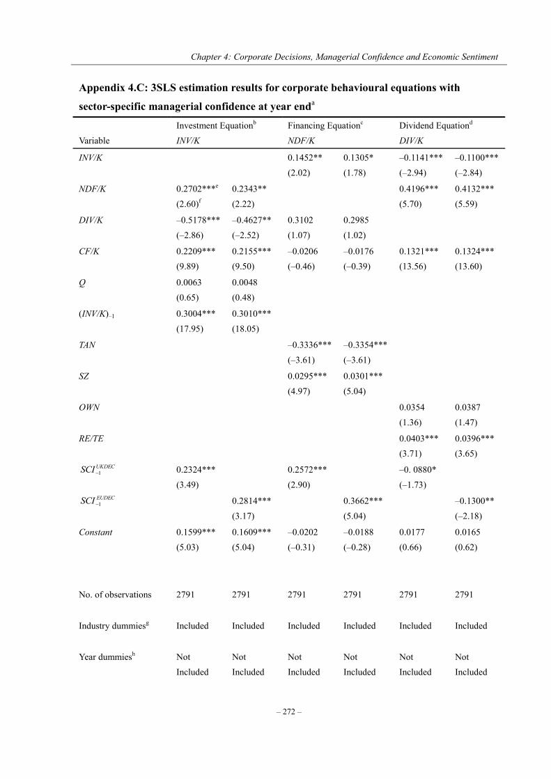
Chapter 4: Corporate Decisions, Managerial Confidence and Economic Sentiment
– 272 –
Appendix 4.C: 3SLS estimation results for corporate behavioural equations with
sector-specific managerial confidence at year enda
Variable Investment Equationb INV/K
Financing Equationc NDF/K
Dividend Equationd DIV/K
INV/K 0.1452** (2.02)
0.1305* (1.78)
–0.1141*** (–2.94)
–0.1100*** (–2.84)
NDF/K 0.2702***e (2.60)f
0.2343** (2.22)
0.4196*** (5.70)
0.4132*** (5.59)
DIV/K –0.5178*** (–2.86)
–0.4627** (–2.52)
0.3102 (1.07)
0.2985 (1.02)
CF/K 0.2209*** (9.89)
0.2155*** (9.50)
–0.0206 (–0.46)
–0.0176 (–0.39)
0.1321*** (13.56)
0.1324*** (13.60)
Q 0.0063 (0.65)
0.0048 (0.48)
(INV/K)–1 0.3004*** (17.95)
0.3010*** (18.05)
TAN –0.3336*** (–3.61)
–0.3354*** (–3.61)
SZ 0.0295*** (4.97)
0.0301*** (5.04)
OWN 0.0354 (1.36)
0.0387 (1.47)
RE/TE 0.0403*** (3.71)
0.0396*** (3.65)
UKDECSCI 1 0.2324*** (3.49)
0.2572*** (2.90)
–0. 0880* (–1.73)
EUDECSCI 1 0.2814*** (3.17)
0.3662*** (5.04)
–0.1300** (–2.18)
Constant 0.1599*** (5.03)
0.1609*** (5.04)
–0.0202 (–0.31)
–0.0188 (–0.28)
0.0177 (0.66)
0.0165 (0.62)
No. of observations
2791 2791 2791 2791 2791 2791
Industry dummiesg
Included Included Included Included Included Included
Year dummiesh
Not Included
Not Included
Not Included
Not Included
Not Included
Not Included
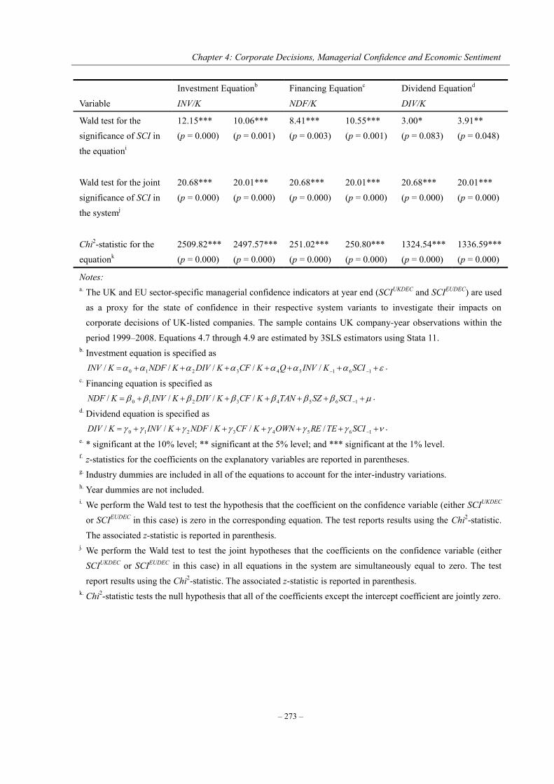
Chapter 4: Corporate Decisions, Managerial Confidence and Economic Sentiment
– 273 –
Variable Investment Equationb INV/K
Financing Equationc NDF/K
Dividend Equationd DIV/K
Wald test for the significance of SCI in the equationi
12.15*** (p = 0.000)
10.06*** (p = 0.001)
8.41*** (p = 0.003)
10.55*** (p = 0.001)
3.00* (p = 0.083)
3.91** (p = 0.048)
Wald test for the joint significance of SCI in the systemj
20.68*** (p = 0.000)
20.01*** (p = 0.000)
20.68*** (p = 0.000)
20.01*** (p = 0.000)
20.68*** (p = 0.000)
20.01*** (p = 0.000)
Chi2-statistic for the equationk
2509.82*** (p = 0.000)
2497.57*** (p = 0.000)
251.02*** (p = 0.000)
250.80*** (p = 0.000)
1324.54*** (p = 0.000)
1336.59*** (p = 0.000)
Notes: a. The UK and EU sector-specific managerial confidence indicators at year end (SCIUKDEC and SCIEUDEC) are used
as a proxy for the state of confidence in their respective system variants to investigate their impacts on corporate decisions of UK-listed companies. The sample contains UK company-year observations within the period 1999–2008. Equations 4.7 through 4.9 are estimated by 3SLS estimators using Stata 11.
b. Investment equation is specified as 161543210 ///// SCIKINVQKCFKDIVKNDFKINV .
c. Financing equation is specified as 16543210 //// SCISZTANKCFKDIVKINVKNDF .
d. Dividend equation is specified as 16543210 ///// SCITEREOWNKCFKNDFKINVKDIV .
e. * significant at the 10% level; ** significant at the 5% level; and *** significant at the 1% level. f. z-statistics for the coefficients on the explanatory variables are reported in parentheses. g. Industry dummies are included in all of the equations to account for the inter-industry variations. h. Year dummies are not included. i. We perform the Wald test to test the hypothesis that the coefficient on the confidence variable (either SCIUKDEC
or SCIEUDEC in this case) is zero in the corresponding equation. The test reports results using the Chi2-statistic. The associated z-statistic is reported in parenthesis.
j. We perform the Wald test to test the joint hypotheses that the coefficients on the confidence variable (either SCIUKDEC or SCIEUDEC in this case) in all equations in the system are simultaneously equal to zero. The test report results using the Chi2-statistic. The associated z-statistic is reported in parenthesis.
k. Chi2-statistic tests the null hypothesis that all of the coefficients except the intercept coefficient are jointly zero.
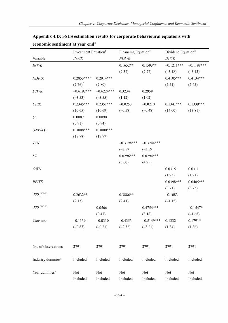
Chapter 4: Corporate Decisions, Managerial Confidence and Economic Sentiment
– 274 –
Appendix 4.D: 3SLS estimation results for corporate behavioural equations with
economic sentiment at year enda
Variable Investment Equationb INV/K
Financing Equationc NDF/K
Dividend Equationd DIV/K
INV/K 0.1652** (2.37)
0.1593** (2.27)
–0.1211*** (–3.18)
–0.1198*** (–3.13)
NDF/K 0.2853***e (2.76)f
0.2914*** (2.80)
0.4105*** (5.51)
0.4134*** (5.45)
DIV/K –0.6192*** (–3.53)
–0.6224*** (–3.55)
0.3234 (1.12)
0.2958 (1.02)
CF/K 0.2345*** (10.65)
0.2351*** (10.69)
–0.0253 (–0.58)
–0.0210 (–0.48)
0.1341*** (14.00)
0.1339*** (13.81)
Q 0.0087 (0.91)
0.0090 (0.94)
(INV/K)–1 0.3008*** (17.78)
0.3000*** (17.77)
TAN –0.3198*** (–3.57)
–0.3244*** (–3.59)
SZ 0.0296*** (5.00)
0.0294*** (4.95)
OWN 0.0315 (1.23)
0.0311 (1.21)
RE/TE 0.0398*** (3.71)
0.0405*** (3.73)
UKDECESI 1 0.2632** (2.13)
0.3886** (2.41)
–0.1083 (–1.15)
EUDECESI 1 0.0566 (0.47)
0.4754*** (3.18)
–0.1547* (–1.68)
Constant –0.1139 (–0.87)
–0.0310 (–0.21)
–0.4353 (–2.52)
–0.5149*** (–3.21)
0.1332 (1.34)
0.1791* (1.86)
No. of observations
2791 2791 2791 2791 2791 2791
Industry dummiesg
Included Included Included Included Included Included
Year dummiesh
Not Included
Not Included
Not Included
Not Included
Not Included
Not Included
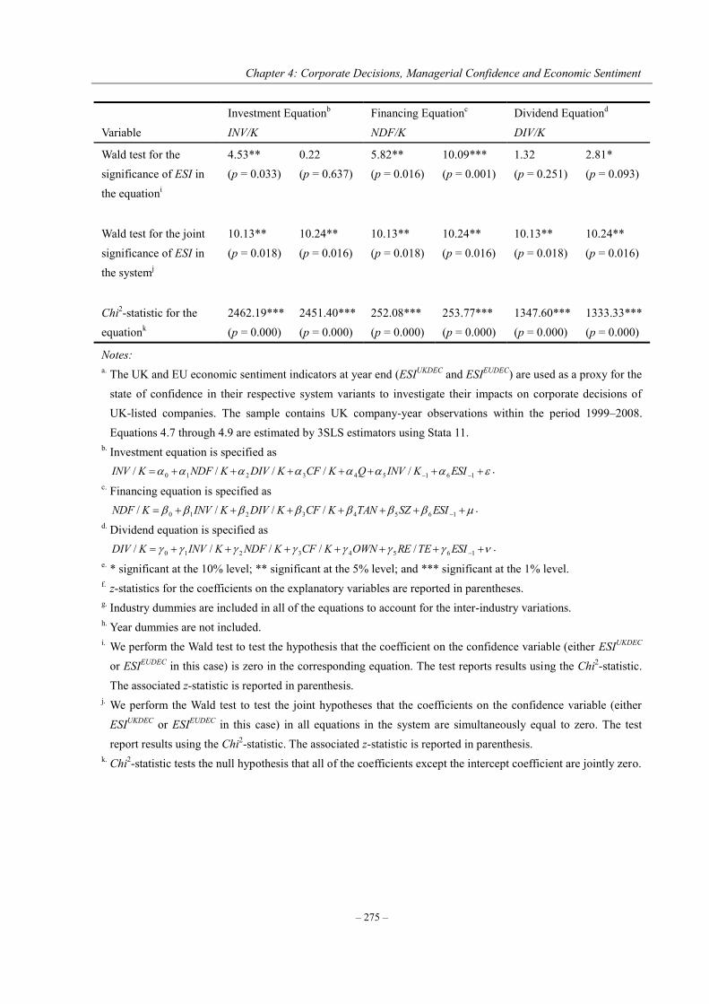
Chapter 4: Corporate Decisions, Managerial Confidence and Economic Sentiment
– 275 –
Variable Investment Equationb INV/K
Financing Equationc NDF/K
Dividend Equationd DIV/K
Wald test for the significance of ESI in the equationi
4.53** (p = 0.033)
0.22 (p = 0.637)
5.82** (p = 0.016)
10.09*** (p = 0.001)
1.32 (p = 0.251)
2.81* (p = 0.093)
Wald test for the joint significance of ESI in the systemj
10.13** (p = 0.018)
10.24** (p = 0.016)
10.13** (p = 0.018)
10.24** (p = 0.016)
10.13** (p = 0.018)
10.24** (p = 0.016)
Chi2-statistic for the equationk
2462.19*** (p = 0.000)
2451.40*** (p = 0.000)
252.08*** (p = 0.000)
253.77*** (p = 0.000)
1347.60*** (p = 0.000)
1333.33*** (p = 0.000)
Notes: a. The UK and EU economic sentiment indicators at year end (ESIUKDEC and ESIEUDEC) are used as a proxy for the
state of confidence in their respective system variants to investigate their impacts on corporate decisions of UK-listed companies. The sample contains UK company-year observations within the period 1999–2008. Equations 4.7 through 4.9 are estimated by 3SLS estimators using Stata 11.
b. Investment equation is specified as 161543210 ///// ESIKINVQKCFKDIVKNDFKINV .
c. Financing equation is specified as 16543210 //// ESISZTANKCFKDIVKINVKNDF .
d. Dividend equation is specified as 16543210 ///// ESITEREOWNKCFKNDFKINVKDIV .
e. * significant at the 10% level; ** significant at the 5% level; and *** significant at the 1% level. f. z-statistics for the coefficients on the explanatory variables are reported in parentheses. g. Industry dummies are included in all of the equations to account for the inter-industry variations. h. Year dummies are not included. i. We perform the Wald test to test the hypothesis that the coefficient on the confidence variable (either ESIUKDEC
or ESIEUDEC in this case) is zero in the corresponding equation. The test reports results using the Chi2-statistic. The associated z-statistic is reported in parenthesis.
j. We perform the Wald test to test the joint hypotheses that the coefficients on the confidence variable (either ESIUKDEC or ESIEUDEC in this case) in all equations in the system are simultaneously equal to zero. The test report results using the Chi2-statistic. The associated z-statistic is reported in parenthesis.
k. Chi2-statistic tests the null hypothesis that all of the coefficients except the intercept coefficient are jointly zero.
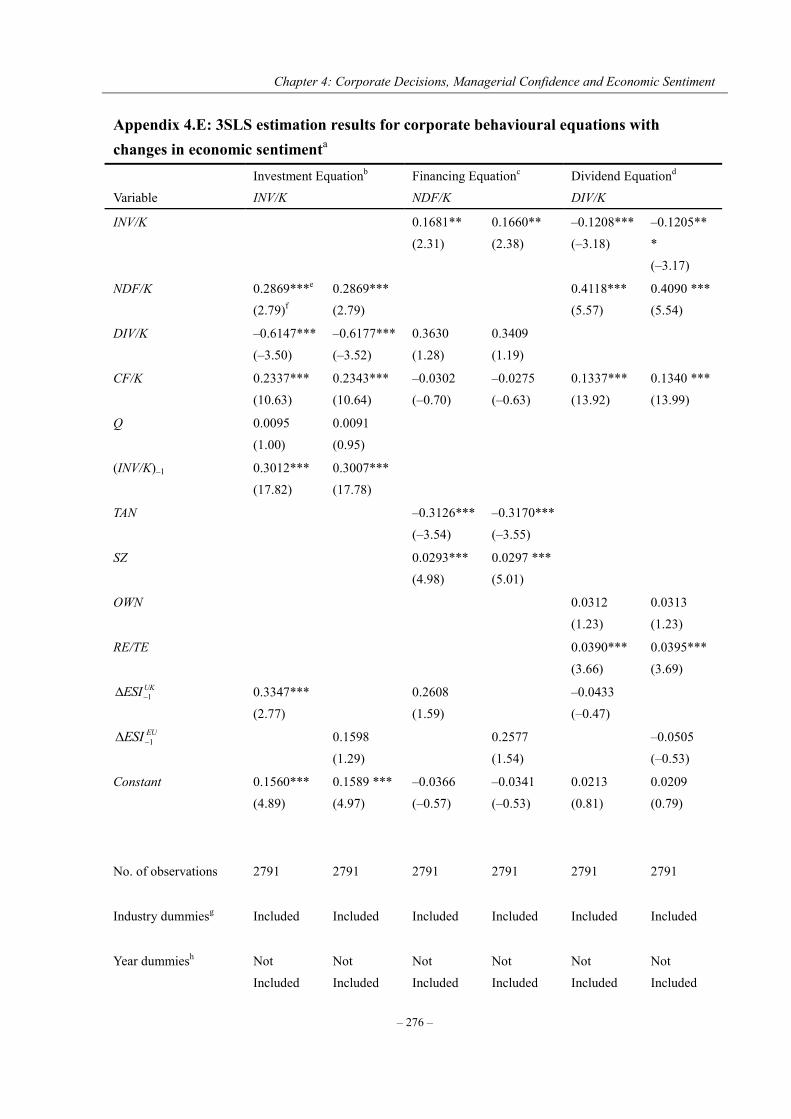
Chapter 4: Corporate Decisions, Managerial Confidence and Economic Sentiment
– 276 –
Appendix 4.E: 3SLS estimation results for corporate behavioural equations with changes in economic sentimenta
Variable Investment Equationb INV/K
Financing Equationc NDF/K
Dividend Equationd DIV/K
INV/K 0.1681** (2.31)
0.1660** (2.38)
–0.1208*** (–3.18)
–0.1205*** (–3.17)
NDF/K 0.2869***e (2.79)f
0.2869*** (2.79)
0.4118*** (5.57)
0.4090 *** (5.54)
DIV/K –0.6147*** (–3.50)
–0.6177*** (–3.52)
0.3630 (1.28)
0.3409 (1.19)
CF/K 0.2337*** (10.63)
0.2343*** (10.64)
–0.0302 (–0.70)
–0.0275 (–0.63)
0.1337*** (13.92)
0.1340 *** (13.99)
Q 0.0095 (1.00)
0.0091 (0.95)
(INV/K)–1 0.3012*** (17.82)
0.3007*** (17.78)
TAN –0.3126*** (–3.54)
–0.3170*** (–3.55)
SZ 0.0293*** (4.98)
0.0297 *** (5.01)
OWN 0.0312 (1.23)
0.0313 (1.23)
RE/TE 0.0390*** (3.66)
0.0395*** (3.69)
UKESI 1 0.3347*** (2.77)
0.2608 (1.59)
–0.0433 (–0.47)
EUESI 1 0.1598 (1.29)
0.2577 (1.54)
–0.0505 (–0.53)
Constant 0.1560*** (4.89)
0.1589 *** (4.97)
–0.0366 (–0.57)
–0.0341 (–0.53)
0.0213 (0.81)
0.0209 (0.79)
No. of observations
2791 2791 2791 2791 2791 2791
Industry dummiesg
Included Included Included Included Included Included
Year dummiesh
Not Included
Not Included
Not Included
Not Included
Not Included
Not Included
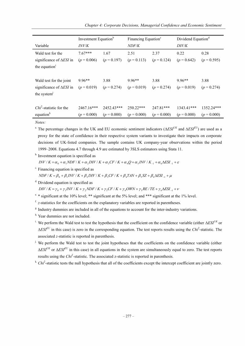
Chapter 4: Corporate Decisions, Managerial Confidence and Economic Sentiment
– 277 –
Variable Investment Equationb INV/K
Financing Equationc NDF/K
Dividend Equationd DIV/K
Wald test for the significance of ∆ESI in the equationi
7.67*** (p = 0.006)
1.67 (p = 0.197)
2.51 (p = 0.113)
2.37 (p = 0.124)
0.22 (p = 0.642)
0.28 (p = 0.595)
Wald test for the joint significance of ∆ESI in the systemj
9.96** (p = 0.019)
3.88 (p = 0.274)
9.96** (p = 0.019)
3.88 (p = 0.274)
9.96** (p = 0.019)
3.88 (p = 0.274)
Chi2-statistic for the equationk
2467.16*** (p = 0.000)
2452.43*** (p = 0.000)
250.22*** (p = 0.000)
247.81*** (p = 0.000)
1343.41*** (p = 0.000)
1352.24*** (p = 0.000)
Notes: a. The percentage changes in the UK and EU economic sentiment indicators (∆ESIUK and ∆ESIEU) are used as a
proxy for the state of confidence in their respective system variants to investigate their impacts on corporate decisions of UK-listed companies. The sample contains UK company-year observations within the period 1999–2008. Equations 4.7 through 4.9 are estimated by 3SLS estimators using Stata 11.
b. Investment equation is specified as 161543210 ///// ESIKINVQKCFKDIVKNDFKINV
c. Financing equation is specified as 16543210 //// ESISZTANKCFKDIVKINVKNDF
d. Dividend equation is specified as 16543210 ///// ESITEREOWNKCFKNDFKINVKDIV
e. * significant at the 10% level; ** significant at the 5% level; and *** significant at the 1% level. f. z-statistics for the coefficients on the explanatory variables are reported in parentheses. g. Industry dummies are included in all of the equations to account for the inter-industry variations. h. Year dummies are not included. i. We perform the Wald test to test the hypothesis that the coefficient on the confidence variable (either ∆ESIUK or
∆ESIEU in this case) is zero in the corresponding equation. The test reports results using the Chi2-statistic. The associated z-statistic is reported in parenthesis.
j. We perform the Wald test to test the joint hypotheses that the coefficients on the confidence variable (either ∆ESIUK or ∆ESIEU in this case) in all equations in the system are simultaneously equal to zero. The test reports results using the Chi2-statistic. The associated z-statistic is reported in parenthesis.
k. Chi2-statistic tests the null hypothesis that all of the coefficients except the intercept coefficient are jointly zero.

Chapter 4: Corporate Decisions, Managerial Confidence and Economic Sentiment
– 278 –
Appendix 4.F: 2SLS estimation results for corporate behavioural equations with
sector-specific managerial confidencea
Variable Investment Equationb INV/K
Financing Equationc NDF/K
Dividend Equationd DIV/K
INV/K 0.0503 (1.54)
0.0369 (1.48)
–0.1081*** (–2.80)
–0.1045*** (–2.56)
NDF/K 0.2413**e (2.31)f
0.2111** (1.98)
0.4743*** (6.14)
0.4718*** (6.06)
DIV/K –0.3812** (–2.10)
–0.3536* (–1.91)
0.1231 (1.26)
0.1225 (1.24)
CF/K 0.2036*** (9.12)
0.2011*** (8.85)
–0.0291 (–0.55)
–0.0313 (–0.58)
0.1265*** (12.43)
0.1266*** (12.39)
Q 0.0129 (1.32)
0.0109 (1.09)
(INV/K)–1 0.3010*** (18.02)
0.2997*** (18.00)
TAN –0.4628*** (–4.40)
–0.4573*** (–3.72)
SZ 0.0423*** (6.75)
0.0423*** (6.72)
OWN 0.0834** (2.55)
0.0857*** (2.61)
RE/TE 0.0505*** (3.88)
0.0487*** (3.77)
UKSCI 1 0.3531*** (4.38)
0.4323*** (3.77)
–0. 1181* (–1.82)
EUSCI 1 0.3890*** (4.33)
0.4056*** (3.44)
–0.1592** (–2.25)
Constant 0.1461*** (4.59)
0.1588*** (4.33)
0.0263 (0.36)
0.0271 (0.37)
–0.0035 (–0.13)
–0.0039 (–0.14)
No. of observations
2791 2791 2791 2791 2791 2791
Industry dummiesg
Included Included Included Included Included Included
Year dummiesh
Not Included
Not Included
Not Included
Not Included
Not Included
Not Included
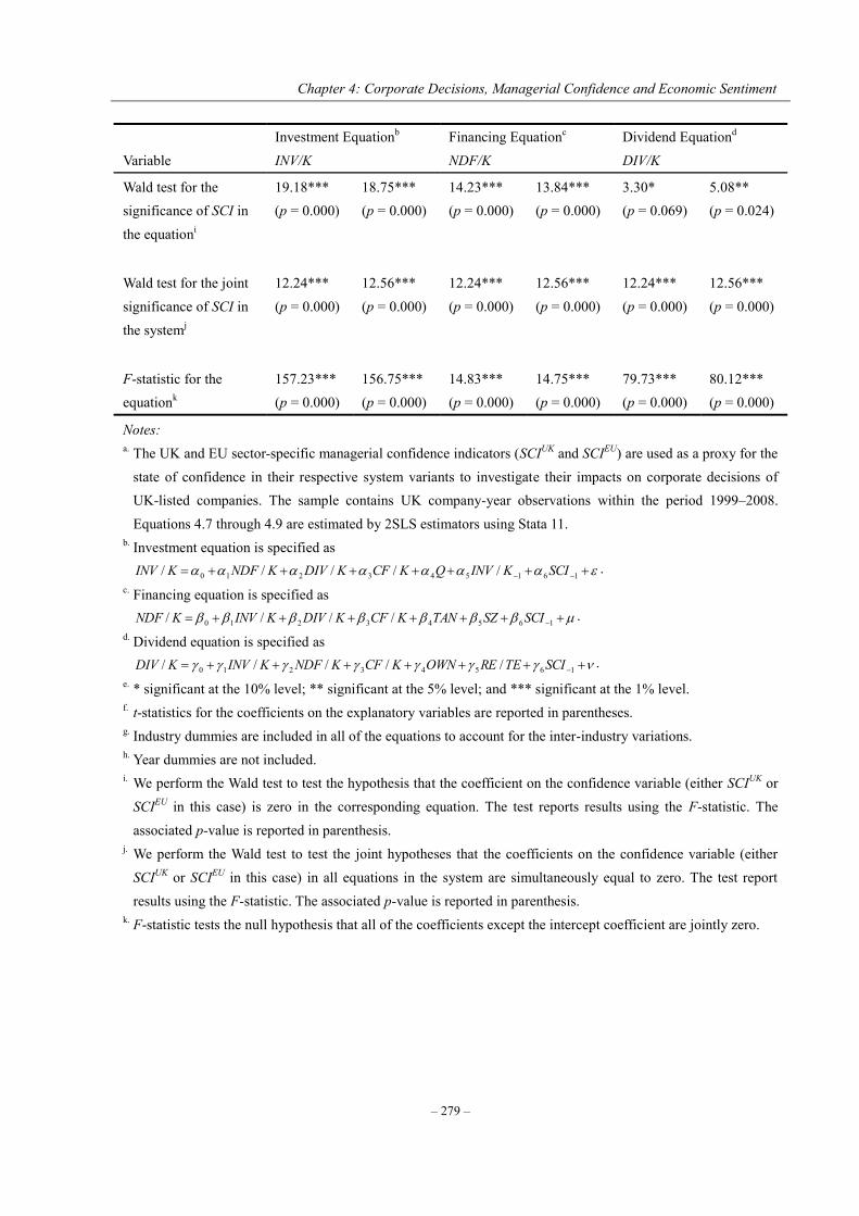
Chapter 4: Corporate Decisions, Managerial Confidence and Economic Sentiment
– 279 –
Variable Investment Equationb INV/K
Financing Equationc NDF/K
Dividend Equationd DIV/K
Wald test for the significance of SCI in the equationi
19.18*** (p = 0.000)
18.75*** (p = 0.000)
14.23*** (p = 0.000)
13.84*** (p = 0.000)
3.30* (p = 0.069)
5.08** (p = 0.024)
Wald test for the joint significance of SCI in the systemj
12.24*** (p = 0.000)
12.56*** (p = 0.000)
12.24*** (p = 0.000)
12.56*** (p = 0.000)
12.24*** (p = 0.000)
12.56*** (p = 0.000)
F-statistic for the equationk
157.23*** (p = 0.000)
156.75*** (p = 0.000)
14.83*** (p = 0.000)
14.75*** (p = 0.000)
79.73*** (p = 0.000)
80.12*** (p = 0.000)
Notes: a. The UK and EU sector-specific managerial confidence indicators (SCIUK and SCIEU) are used as a proxy for the
state of confidence in their respective system variants to investigate their impacts on corporate decisions of UK-listed companies. The sample contains UK company-year observations within the period 1999–2008. Equations 4.7 through 4.9 are estimated by 2SLS estimators using Stata 11.
b. Investment equation is specified as 161543210 ///// SCIKINVQKCFKDIVKNDFKINV .
c. Financing equation is specified as 16543210 //// SCISZTANKCFKDIVKINVKNDF .
d. Dividend equation is specified as 16543210 ///// SCITEREOWNKCFKNDFKINVKDIV .
e. * significant at the 10% level; ** significant at the 5% level; and *** significant at the 1% level. f. t-statistics for the coefficients on the explanatory variables are reported in parentheses. g. Industry dummies are included in all of the equations to account for the inter-industry variations. h. Year dummies are not included. i. We perform the Wald test to test the hypothesis that the coefficient on the confidence variable (either SCIUK or
SCIEU in this case) is zero in the corresponding equation. The test reports results using the F-statistic. The associated p-value is reported in parenthesis.
j. We perform the Wald test to test the joint hypotheses that the coefficients on the confidence variable (either SCIUK or SCIEU in this case) in all equations in the system are simultaneously equal to zero. The test report results using the F-statistic. The associated p-value is reported in parenthesis.
k. F-statistic tests the null hypothesis that all of the coefficients except the intercept coefficient are jointly zero.
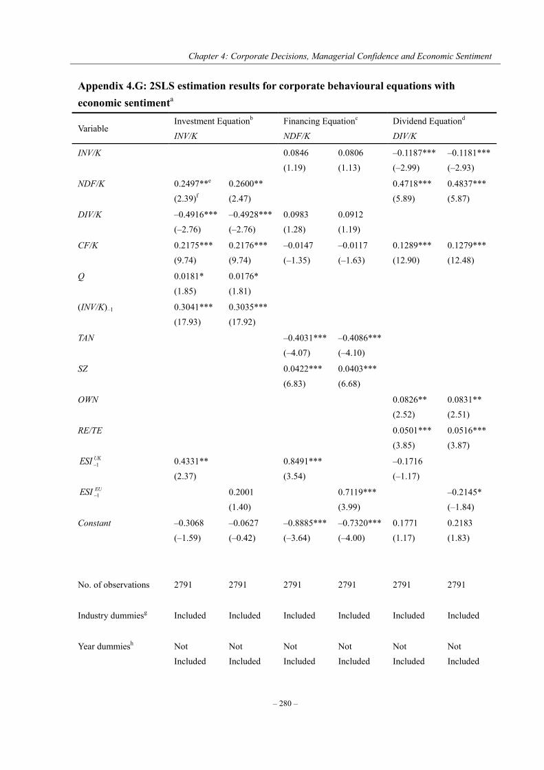
Chapter 4: Corporate Decisions, Managerial Confidence and Economic Sentiment
– 280 –
Appendix 4.G: 2SLS estimation results for corporate behavioural equations with economic sentimenta
Variable Investment Equationb INV/K
Financing Equationc NDF/K
Dividend Equationd DIV/K
INV/K 0.0846 (1.19)
0.0806 (1.13)
–0.1187*** (–2.99)
–0.1181*** (–2.93)
NDF/K 0.2497**e (2.39)f
0.2600** (2.47)
0.4718*** (5.89)
0.4837*** (5.87)
DIV/K –0.4916*** (–2.76)
–0.4928*** (–2.76)
0.0983 (1.28)
0.0912 (1.19)
CF/K 0.2175*** (9.74)
0.2176*** (9.74)
–0.0147 (–1.35)
–0.0117 (–1.63)
0.1289*** (12.90)
0.1279*** (12.48)
Q 0.0181* (1.85)
0.0176* (1.81)
(INV/K)–1 0.3041*** (17.93)
0.3035*** (17.92)
TAN –0.4031*** (–4.07)
–0.4086*** (–4.10)
SZ 0.0422*** (6.83)
0.0403*** (6.68)
OWN 0.0826** (2.52)
0.0831** (2.51)
RE/TE 0.0501*** (3.85)
0.0516*** (3.87)
UKESI 1 0.4331** (2.37)
0.8491*** (3.54)
–0.1716 (–1.17)
EUESI 1 0.2001 (1.40)
0.7119*** (3.99)
–0.2145* (–1.84)
Constant –0.3068 (–1.59)
–0.0627 (–0.42)
–0.8885*** (–3.64)
–0.7320*** (–4.00)
0.1771 (1.17)
0.2183 (1.83)
No. of observations
2791 2791 2791 2791 2791 2791
Industry dummiesg
Included Included Included Included Included Included
Year dummiesh
Not Included
Not Included
Not Included
Not Included
Not Included
Not Included
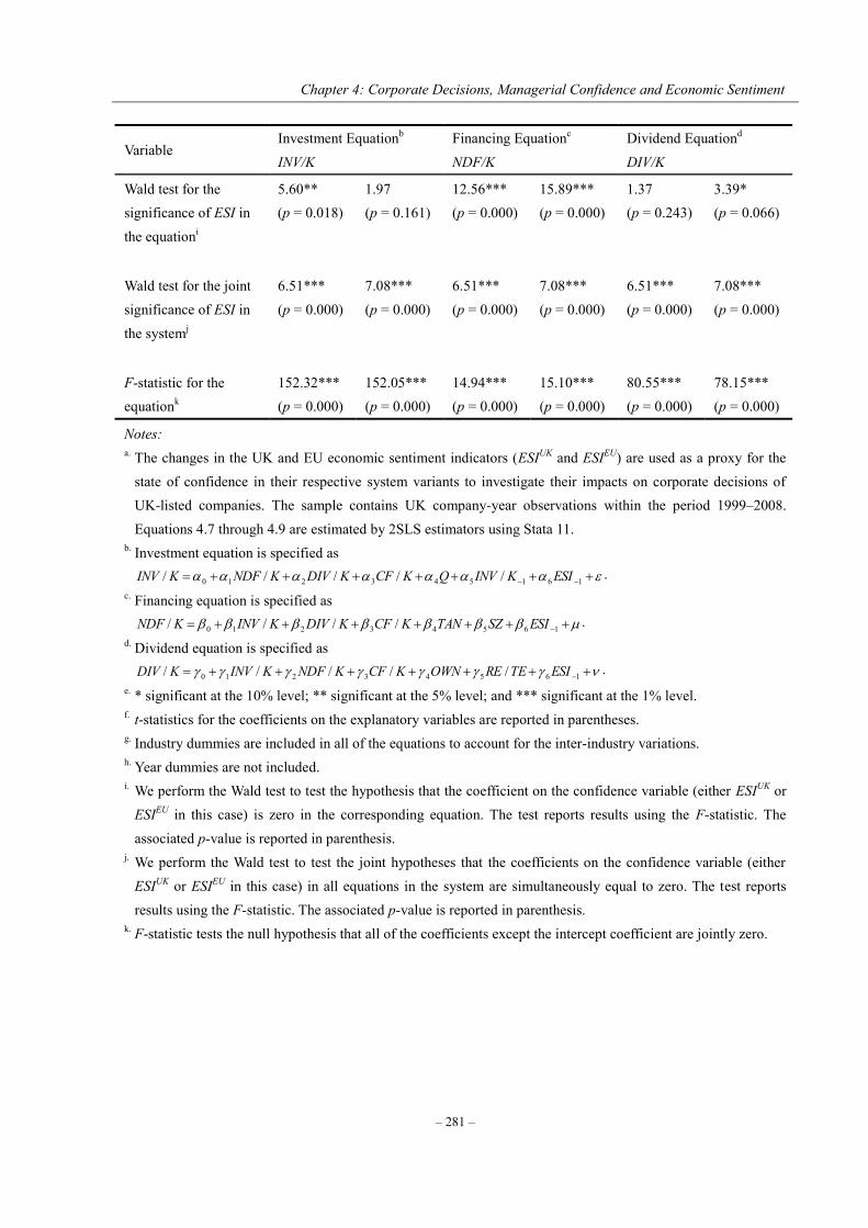
Chapter 4: Corporate Decisions, Managerial Confidence and Economic Sentiment
– 281 –
Variable Investment Equationb INV/K
Financing Equationc NDF/K
Dividend Equationd DIV/K
Wald test for the significance of ESI in the equationi
5.60** (p = 0.018)
1.97 (p = 0.161)
12.56*** (p = 0.000)
15.89*** (p = 0.000)
1.37 (p = 0.243)
3.39* (p = 0.066)
Wald test for the joint significance of ESI in the systemj
6.51*** (p = 0.000)
7.08*** (p = 0.000)
6.51*** (p = 0.000)
7.08*** (p = 0.000)
6.51*** (p = 0.000)
7.08*** (p = 0.000)
F-statistic for the equationk
152.32*** (p = 0.000)
152.05*** (p = 0.000)
14.94*** (p = 0.000)
15.10*** (p = 0.000)
80.55*** (p = 0.000)
78.15*** (p = 0.000)
Notes: a. The changes in the UK and EU economic sentiment indicators (ESIUK and ESIEU) are used as a proxy for the
state of confidence in their respective system variants to investigate their impacts on corporate decisions of UK-listed companies. The sample contains UK company-year observations within the period 1999–2008. Equations 4.7 through 4.9 are estimated by 2SLS estimators using Stata 11.
b. Investment equation is specified as 161543210 ///// ESIKINVQKCFKDIVKNDFKINV .
c. Financing equation is specified as 16543210 //// ESISZTANKCFKDIVKINVKNDF .
d. Dividend equation is specified as 16543210 ///// ESITEREOWNKCFKNDFKINVKDIV .
e. * significant at the 10% level; ** significant at the 5% level; and *** significant at the 1% level. f. t-statistics for the coefficients on the explanatory variables are reported in parentheses. g. Industry dummies are included in all of the equations to account for the inter-industry variations. h. Year dummies are not included. i. We perform the Wald test to test the hypothesis that the coefficient on the confidence variable (either ESIUK or
ESIEU in this case) is zero in the corresponding equation. The test reports results using the F-statistic. The associated p-value is reported in parenthesis.
j. We perform the Wald test to test the joint hypotheses that the coefficients on the confidence variable (either ESIUK or ESIEU in this case) in all equations in the system are simultaneously equal to zero. The test reports results using the F-statistic. The associated p-value is reported in parenthesis.
k. F-statistic tests the null hypothesis that all of the coefficients except the intercept coefficient are jointly zero.

Chapter 5: The Measurement of Corporate Investment Behaviour Matters
– 282 –
CHAPTER 5
THE MEASUREMENT OF CORPORATE INVESTMENT BEHAVIOUR
MATTERS
5.1 Introduction
Corporate investment behaviour is one of the most widely and intensively investigated areas
in corporate finance. As can be seen in Chapter 2, with theoretical developments relating to
corporate investment behaviour has come a large body of literature devoted to empirically
investigating the relations between capital investment decision and relevant company-level
characteristics, such as the investment opportunity set, financial constraints, uncertainty,
managerial confidence, etc. Although the empirical models used to examine corporate
investment behaviour differ in their objectives and approaches, the use of a ratio of corporate
investment to capital stock as the empirical measure of the conceptual variable of corporate
investment behaviour has become a common practice in the literature.
The ratios of corporate investment to capital stock used in the literature, which seem at
first sight to be very similarly specified, are in fact different both on the numerator and the
denominator. Specifically, corporate investment spending has been empirically measured
using a wide range of methods, either based on a cash flow statement or a balance sheet,
either on a gross or net basis, and either with or without considering disinvestment.
Meanwhile, capital stock has also been proxied in a number of different ways, either using
Chapter 5: The Measurement of Corporate Investment Behaviour Matters
– 283 –
tangible fixed assets or total assets, either based on book value or replacement value, either
with or without taking a time lag. The combinations of different measures of corporate
investment spending alongside various proxies for capital stock generate numerous ways in
which the ratio of corporate investment to capital stock can be specified, making the
measurement of corporate investment behaviour even more problematic.
At least twenty different versions of corporate investment to capital stock ratio
calculations have been identified in the existing literature. However, no attempt has been
made to provide a comparison among various corporate investment measures. One claim
which has been implicitly made is that different measures of corporate investment behaviour
will always yield the same, or at least qualitatively similar, results in empirical analyses. As a
consequence, we know little about how differently these corporate investment measures
perform in empirical analyses, and the extent to which the choice of corporate investment
measures may influence the conclusions drawn from the analyses. Therefore, the purpose of
this chapter is to fill the gap by conceptually discriminating and empirically evaluating twenty
alternative measures of corporate investment behaviour which are currently used in the
literature.
Using data from a balanced panel of 432 UK-listed companies over the period
1999–2008, this chapter discriminates conceptually and evaluates empirically twenty
alternative measures of corporate investment behaviour, contributing to the existing literature
in a number of ways. First, this chapter calls attention to the potential misuse of numerous
Chapter 5: The Measurement of Corporate Investment Behaviour Matters
– 284 –
corporate investment measures in applied corporate finance research. The question of whether
the measurement of corporate investment behaviour matters, which has never been raised, is
empirically addressed in this chapter. Second, this chapter highlights the distinctions between
accrual based and cash flow based corporate investment measures as well as between gross
and net corporate investment measures from an accounting perspective, providing insight into
the fundamental differences among the similarly specified alternatives. Third, using a large
panel of UK-listed companies, this chapter empirically evaluates the performance of the
alternative investment measures in terms of their volatility and information content. The
evaluation results are of great interest to corporate finance researchers as well as other users
of financial statements. Furthermore, based on the evaluation results, we suggest a set of best
performing measures of corporate investment behaviour, which are less noisy and more
informative, for researchers to utilise. Taking all the innovations together, this chapter may
shed some light and provide some guidance for measuring corporate investment behaviour in
empirical analyses.
The remainder of this chapter is organised as follows. Section 5.2 highlights and
explains the differences among various corporate investment measures utilised in the existing
empirical literature. Section 5.3 develops a number of testable hypotheses. Section 5.4
describes the sample selection, corporate investment measures, and preliminary analysis.
Section 5.5 offers an illustrative example to determine the extent to which the choice of
corporate investment measures influences the conclusions drawn from empirical analyses.
Chapter 5: The Measurement of Corporate Investment Behaviour Matters
– 285 –
Sections 5.6 and 5.7 assess the volatility around the trends and the information content of the
corporate investment measures, respectively. Concluding remarks are drawn in Section 5.8.
5.2 Empirical measures of corporate investment behaviour
Although the relevant literature has been reviewed in Chapter 2, it is useful to highlight the
key aspects of the literature that illustrate the numerous corporate investment measures that
are in vogue in empirical works. As can be seen in Chapter 2, corporate investment decisions
play an important role in maintaining and increasing the scope of a company’s operations, and
have been the focus of a large amount of academic research. Existing literature in corporate
finance mainly focuses on the effect of relevant company characteristics, such as investment
opportunity set (see Carpenter and Guariglia, 2008), internal financial constraints (see
Guariglia, 2008; Cummins et al., 2006; and Barran and Peeters, 1998), external financial
constraints (see Guariglia, 2008; and Aggarwal and Zong, 2006), information asymmetry (see
Ascioglu et al., 2008), managerial optimism (see Ben-David et al., 2007; and Malmendier and
Tate, 2005), and uncertainty (see Baum et al., 2008; and Lensink and Murinde, 2006), on
corporate investment behaviour. Conflicting empirical evidence obtained from the
tremendous amount of literature induces intense debates upon almost all aspects of corporate
investment behaviour. For example, Fazzari et al. (1988) and Ascioglu et al. (2008), among
many others, find a higher sensitivity of corporate investment to cash flow for companies that
are more likely to be financially constrained, whereas Kaplan and Zingales (1997), Cleary
(1999) and some others find the opposite. Abdul-Haque and Wang (2008) and Lensink and
Chapter 5: The Measurement of Corporate Investment Behaviour Matters
– 286 –
Sterken (2000) find a positive effect of company-specific uncertainty on corporate investment,
whereas Bloom et al. (2007), Xie (2009) and many others find the opposite. Some innovative
models, therefore, have been developed in an attempt to reconcile the conflicting findings
from theoretical points of view (see, for example, Cleary et al., 2007; and Sarkar, 2000).
However, to the best of our knowledge, no attention has been directed to the
measurement of corporate investment behaviour in the existing literature. The equation of
whether the measurement of corporate investment behaviour matters has never been raised.
One claim which has been implicitly made is that the different measures of corporate
investment behaviour are equivalent to one another, and can be used interchangeably. Thus we
know little about how differently the measures of corporate investment perform in applied
studies, and the extent to which the choice for measuring corporate investment influences the
results of empirical analyses. Although corporate investment is customarily measured by the
ratio of corporate investment to capital stock, the seemingly similarly specified investment
ratios actually vary both on the numerator and on the denominator. Therefore, it is reasonable
to posit that the conflicting conclusions drawn from the existing literature on corporate
investment may partly be attributable to the differences in measuring companies’ investment
behaviour.
Twenty different versions of corporate investment to capital stock ratio specifications,
ranging from simply constructed measures based on reported accounting items to relatively
complex measures which involve estimating the replacement value of capital stock, have been
Chapter 5: The Measurement of Corporate Investment Behaviour Matters
– 287 –
identified in the recent empirical works published in highly cited academic journals.46
Different measures of capital investment spending alongside various proxies for capital stock
are used in the specification of these investment ratios. As pointed out by Adam and Goyal
(2008), the lack of understanding of measurements is a crucial problem in empirical corporate
finance research. Likewise, the potential misuse of corporate investment measures in the
applied corporate finance literature may also be largely due to a lack of understanding of the
financial information provided by relevant accounting items. Therefore, the starting point for
conceptually discriminating various measures of corporate investment should be their
respective accounting definitions.
5.2.1 Cash based versus accrual based corporate investment measures
Corporate investment refers to the amount of investment made by a company to its capital
stock during certain period of time. The measurement of corporate investment relies heavily
on the relevant accounting information reported in a company’s financial statements. More
specifically, a measure of corporate investment can either be taken directly from a cash flow
statement or be derived indirectly from a balance sheet. Given the fact that different
accounting principles are involved in the preparation of cash flow statements and balance
sheets, corporate investment measures can be classified into two broad categories, namely,
cash based and accrual based measures.
46 The studies, from which different corporate investment to capital stock ratios are identified, are all published in journals listed in the Association of Business School’s (ABS) Academic Journal Quality Guide. Most of them are published in journals that are rated as 4*, 4, or 3 by ABS. A list of cited studies can be found in Table 5.1.

Chapter 5: The Measurement of Corporate Investment Behaviour Matters
– 288 –
5.2.1.1 Cash based corporate investment measures
The most commonly used measures of corporate investment in the existing literature are
based on capital expenditures (CAPX) which is a reported item on a company’s cash flow
statement under the investing subsection (see, for example, Grundy and Li, 2010; Bakke and
Whited, 2010; Denis and Sibilkov, 2010; Adam, 2009; Hovakimian and Titman, 2006; etc.).
Since cash flow statements are prepared using the cash basis accounting method, the measures
of corporate investment based on the cash flow statement item of capital expenditures can be
classified as cash based measures.
A cash flow statement is concerned with inflows and outflows of cash and cash
equivalent of a company, without considering transactions that do not directly affect cash
receipts and payments. The capital expenditures item reported on a cash flow statement
represents the funds used by a company to acquire fixed assets and those associated with the
acquisitions over the reporting period. Under cash basis accounting, capital expenditures are
recognised immediately at historical costs when cash is paid out either to buy fixed assets or
to add to the value of an existing fixed asset. Therefore, the capital expenditures item showing
up on a company’s cash flow statement can be adopted directly as a measure of the amount of
funds spent by a company on its capital stock over the reporting period. It is worth noting that,
according to International Accounting Standard (IAS) 7, the funds used to acquire fixed assets
associated with acquisitions are not included in capital expenditures.
The main advantage of using the reported capital expenditures to measure corporate
Chapter 5: The Measurement of Corporate Investment Behaviour Matters
– 289 –
investment is that the cash based figures are less subject to distortions from differing
accounting practices, and thus are able to more objectively reflect a company’s investing
activities (Dechow, 1994). However, a fundamental drawback of cash based investment
measures is that cash flows have timing and mismatching problems which may cause them to
be noisy (Dechow, 1994). Specifically, capital expenditures under cash basis accounting are
recognised when cash is paid out to purchase a fixed asset, regardless of whether the fixed
asset is in place. To mitigate the timing and mismatching problems of cash based figures, the
accrual basis accounting method has been implemented to alter the timing of cash flow
recognition, aiming to more closely reflect business activities.
5.2.1.2 Accrual based corporate investment measures
Instead of using cash based measures, a body of literature derives measures of corporate
investment from a company’s balance sheet, using the book value of tangible fixed assets (see,
for example, Engel and Middendorf, 2009; Guariglia, 2008; Gan, 2007; and Lensink and
Murinde, 2006).47 Tangible fixed assets are also referred to as property, plant and equipment
which can be found on a company’s balance sheet under the non-current assets section. The
difference in the carrying amount of tangible fixed assets (NPPE) between the end and
beginning of a period, therefore, reflects net additions to the availability of a company’s
capital assets. Since balance sheets are prepared under accrual basis accounting, corporate
47 In most cases, only tangible assets are referred to as fixed.

Chapter 5: The Measurement of Corporate Investment Behaviour Matters
– 290 –
investment measures derived from the balance sheet item of property, plant and equipment
can be classified as accrual based measures.
Accrual basis accounting is a method that measures the financial position and
performance of a company by recognising economic events regardless of when cash
transactions occur. Because it is supposed to provide a more accurate picture of a company’s
current financial conditions by reducing noise from timing mismatches between when cash is
paid out and when an asset is recognised, accrual basis accounting has been generally
accepted as the standard accounting practice for most businesses. Under accrual basis
accounting, a capital asset is recognised as a historical cost when it is incurred, and reflected
as an addition to tangible fixed assets on the balance sheet.48 Since accrual basis accounting
mitigates the timing and matching problems of cash flows, accrual based corporate investment
measures should be able to more closely reflect net additions to the availability of a
company’s capital assets.
However, the implementation of accrual basis accounting creates a new set of
problems. Previous studies question the reliability and relevance of accrual basis accounting
figures because of the accrual components (see, for example, Wilson, 1986). It is argued that
management typically have some discretion over the recognition of accruals, and this
discretion might be used by management to opportunistically manipulate the reported
accounting figures, including the carrying amount of tangible fixed assets. The managerial
48 The historical cost of a tangible fixed asset is subject to revaluations and writedowns.
Chapter 5: The Measurement of Corporate Investment Behaviour Matters
– 291 –
manipulation of accruals, therefore, may reduce the credibility and relevance of accrual based
investment measures. In addition, the accrual based investment measures are likely to be
distorted by asset revaluations and writedowns. Both revaluations and writedowns of fixed
assets are different from planned depreciation in the sense that they aim to bring the fair
market value of the capital goods into the books. However, it is found that, in practice, the
most important determinant of writedown decisions is changes in senior management (Strong
and Meyer, 1987). Thus, the accrual based measures of corporate investment derived from
balance sheet are more vulnerable to managers’ opportunistic manipulation. The question of
whether the net effect of accruals is to improve or reduce the ability of investment measures
to reflect business investment behaviour must be addressed empirically.
The use of accrual based measures of corporate investment is mainly driven by a
number of considerations. First, cash based measures of capital expenditures are not always
readily available. Some studies utilise the first difference of tangible fixed assets as a proxy
for corporate investment spending simply because no any independent estimate of corporate
investment, such as reported capital expenditures, is available to the public in the market
being investigated (see, for example, Garcia-Marco and Ocana, 1999). Second, some
theoretical considerations may lead naturally to the use of balance sheet-based measures of
corporate investment. For example, the accelerator model of corporate investment asserts that
a company’s capital stock should be proportional to its level of production, and companies
engage in capital investment in an attempt to close the gap between the desired level of capital

Chapter 5: The Measurement of Corporate Investment Behaviour Matters
– 292 –
stock and the existing level of capital stock left over from the previous period. Accordingly,
empirical investment equations formulated based on the accelerator model typically specify
the change in capital stock of a company as a function of the change in the company’s output
over the same period. The first difference transformation of tangible fixed assets, therefore,
can be utilised as an ideal approximation of the change in capital stock and employed in the
accelerator model of investment as the dependent variable (see, for example, Engel and
Middendorf, 2009; Bo and Lensink, 2005). In addition, a strand of literature based on the
flow-of-funds framework for corporate behaviour also tends to measure corporate investment
using balance sheet items (see, for example, Mougoué and Mukherjee, 1994; Fama, 1974; and
Dhrymes and Kurz, 1967). This is because the budget constraint that overrides the
flow-of-funds framework for corporate behaviour is essentially derived from the accounting
identity that change in assets must equal the sum of changes in liability and equity.
A few studies also consider using the changes in total assets as a proxy for capital
investment (see, for example, Adedeji, 1998). However, it is generally believed that the
changes in total assets that arise from changes in its elements of current assets, such as
accounts receivable and inventories, are likely to be triggered by economic conditions, and
thus cannot be interpreted as the results of corporate investment decisions made by
management (see, for example, Kadapakkam et al., 1998). By contrast the changes in tangible
fixed assets, which focus on investment in property, plant and equipment, should be better
able to reflect the conscious investment decisions taken by management.
Chapter 5: The Measurement of Corporate Investment Behaviour Matters
– 293 –
To sum up, cash basis accounting is fundamentally different from accrual basis
accounting (see Salmi et al., 1990). Since different accounting principles are involved in the
preparation of the accounting items used to empirically measure a company’s investment
spending, accrual based measures of corporate investment may contain information about a
company’s investing activities which is not present in their cash based counterparts, and vice
versa. Therefore, it is meaningful to investigate whether cash based and accrual based
measures of corporate investment behaviour perform similarly in empirical analyses.
5.2.2 Gross versus net corporate investment measures
In accounting, a capital expenditure is required to be capitalised and recorded as a tangible
fixed asset on a company’s balance sheet. According to the basic matching principle of
accounting, the tangible fixed asset is then required to be depreciated over its useful life,
allocating its cost as a depreciation expense to the periods in which the asset is expected to be
used. Therefore, both cash based and accrual based measures of corporate investment
behaviour can be adjusted to be either gross investment measures (see, for example, Grundy
and Li, 2010; Carpenter and Guariglia, 2008; Guariglia, 2008; and Lensink and Murinde,
2006) or net investment measures (see, for example, Denis and Sibilkov, 2010; Wang et al.,
2009; Firth et al., 2008; and Rousseau and Kim, 2008), by adding or netting depreciation,
depletion and amortisation expense (DDA) recognised in the corresponding period.
According to Standard Accounting Statement (SAS) 3 and IAS 16, the value of a

Chapter 5: The Measurement of Corporate Investment Behaviour Matters
– 294 –
tangible fixed asset is required to be carried at its net book value, which is essentially the
difference between the historical cost of the asset and its associated accumulated
depreciation.49 Thus, by definition, the carrying amount of tangible fixed assets reported on a
balance sheet has already taken depreciated capital goods into account. The accrual based
corporate investment measures, which are simply calculated as the first difference of the
carrying amount of tangible fixed assets, therefore represent net additions to the availability of
a company’s capital goods, and can be classified as net investment measures. Accrual based
gross investment measures can be obtained by adding depreciation expense charged over the
period back to the change in the carrying amount of tangible fixed assets. Gross investment
measures, thus, are concerned with the overall investment in capital stock made by a company
over a period. The use of the change in carrying amount of tangible fixed assets to measure
net corporate investment is observed in Chow et al. (2010), Wang et al. (2009), Rousseau and
Kim (2008), Mueller and Peev (2007), etc.; while the use of the sum of the change in the
carrying amount of tangible fixed assets and depreciation expenses to measure gross corporate
investment is adopted by Engel and Middendorf (2009), Guariglia (2008), Bo (2007), Lensink
and Murinde (2006), etc.
Turing to cash based corporate investment measures, the reported capital expenditures
item on the cash flow statement represents the funds spent by a company both to acquire new
49 The net book value of tangible fixed assets is considered the best way of consciously presenting the true and fair value of capital assets to the owner of the business and other users of the financial statements.

Chapter 5: The Measurement of Corporate Investment Behaviour Matters
– 295 –
fixed capital assets and to maintain or upgrade existing tangible fixed assets, without
considering the non-cash expenses such as depreciation. Thus, the reported capital
expenditures can be used directly to construct cash based gross investment measures. This
type of gross corporate investment measure is utilised by a large number of applied studies
(see, for example, Grundy and Li, 2010; Bakke and Whited, 2010; Brown and Petersen, 2009;
Carpenter and Guariglia, 2008; Ratti et al., 2008; Cummins et al., 2006; etc.). Cash based net
investment measures can be easily obtained by subtracting depreciation expense charged for
the reporting period from the amount of total spending on capital goods over the same period.
The use of cash based net investment measures can be found in Denis and Sibilkov (2010),
Firth et al. (2008), Cleary (1999), etc.
Besides, some studies, such as Kang et al.(2010), Bloom et al. (2007), Hennessy et
al.(2007) and Lin et al. (2005), define corporate investment as the net spending on fixed
assets (NSFA), in an attempt to construct a relatively more accurate measure which captures
both capital investment and disinvestment, using cash based accounting figures. Accordingly,
they compute the difference between capital expenditures (CAPX) and revenue from sales of
property, plant and equipment (SPPE), both of which can be found on the cash flow statement
under the investing activities subsection, as a measure of net spending on fixed assets. The net
spending on fixed assets takes proceeds from the sale of fixed assets into account, and thus
could take both positive and negative signs.

Chapter 5: The Measurement of Corporate Investment Behaviour Matters
– 296 –
5.2.3 Book versus replacement values of capital stock
To account for heteroscedasticity across companies, capital investment spending is typically
normalised by a proxy for capital stock to construct a ratio of corporate investment to capital
stock. The book value of net tangible fixed assets (K) and book value of total assets (TA) on
the balance sheet are often chosen as proxies for capital stock to normalise the investment
measures. The use of book value of net tangible fixed assets to scale capital investment is
adopted by the majority of applied studies, such as Chow et al. (2010), Grundy and Li (2010),
Engel and Middendorf (2009), Ratti et al. (2008), Hennessy et al. (2007), etc. Bond and
Meghir (1994) argue that book value of net tangible fixed assets is preferred because it is
relatively more stable over time and less likely to be distorted by economic conditions. The
use of book value of total assets can be observed in Bakke and Whited (2010), Denis and
Sibilkov (2010), Kang et al. (2010), Wang et al. (2009), etc. Brown and Petersen (2009)
argue that the book value of total assets is chosen because they wish to maintain a common
scale factor for all regressors, including research and development expenditures. Therefore,
the choice between book value of tangible fixed assets and that of total assets as a proxy for
capital stock is largely determined by the model specification.
Given the fact that the books record the historical costs of capital goods, which may
deviate from their fair market values, it is also common to derive a replacement value of
capital stock (Kr) from the book value of tangible fixed assets (see, for example, Guariglia,
2008; Baum et al., 2008; Bloom et al., 2007; Cummins et al., 2006; etc.). Replacement value
Chapter 5: The Measurement of Corporate Investment Behaviour Matters
– 297 –
of capital stock is preferred by some researchers because it represents the actual cost to
replace the current productive capacity of a company at the present time. Replacement value,
however, is difficult to estimate in the absence of active markets for used capital goods
(Perfect and Wiles, 1994). In practice, replacement value of capital stock is conventionally
estimated using a standard perpetual inventory method initially proposed by Salinger and
Summers (1983). Under the standard perpetual inventory method, the book value of tangible
fixed assets is treated as the historical value of the capital stock. The replacement value and
historical value are assumed to be the same in the first year of data, which is then adjusted for
each following period in accordance with the corresponding price deflator of non-residential
investment goods (see Appendix 5.A for a detailed explanation of the perpetual inventory
method). Because the price level for capital goods normally increases over time, the
replacement value of capital stock estimated using the perpetual inventory method is typically
greater than the corresponding book value. However, owing to the assumptions necessary to
implement the estimation, the standard perpetual inventory procedure may lead to negative
replacement value of capital stock in certain instances, which is intuitively undesirable.
5.2.4 Contemporaneous versus lagged proxies for capital stock
Researchers also face a choice between contemporaneous or lagged deflator when they
construct a ratio of corporate investment to capital stock. Some studies choose to use a
contemporaneous proxy for capital stock as the deflator of corporate investment in an attempt
to make full use of their company-year observations and maximise sample size for their
Chapter 5: The Measurement of Corporate Investment Behaviour Matters
– 298 –
analyses (see, for example, Bakke and Whited, 2010; Ratti et al., 2008; Firth et al., 2008; and
Lensink and Murinde, 2006); while others argue that all of the investment decisions are made
at the beginning of each fiscal year, and thus it is more appropriate to use the
beginning-of-period value of capital stock to deflate corporate investment, especially for
companies with substantial growth over the sample period. In addition, the use of lagged
proxy for capital stock can effectively reduce the possibility of using more information in
modelling corporate investment behaviour than managers actually have when they make their
decisions. However, if a lagged proxy for capital stock is chosen to construct corporate
investment measures, the first year observation for each company has to be sacrificed, leading
to relatively lower degrees of freedom for regression analyses. The use of corporate
investment to lagged capital stock ratios can be found in Grundy and Li (2010), Chow et al.
(2010), Denis and Sibilkov (2010), Kang et al. (2010), etc.
5.2.5 Conclusion
The review of relevant literature shows that, although the use of corporate investment to
capital stock ratio to measure companies’ investment behaviour has become common practice
in applied studies, there is no consensus about how the ratio should be empirically specified.
The combinations of different measures of capital investment spending alongside various
proxies for capital stock generate a large number of ways in which the ratio of corporate
investment to capital stock can be specified. More importantly, given the fact that different
accounting principles are involved in the preparation of relevant accounting items used to
Chapter 5: The Measurement of Corporate Investment Behaviour Matters
– 299 –
measure corporate investment behaviour, corporate investment to capital stock ratios with
different specifications are likely to carry different information about a company’s investing
activities. The implicit assumption that different corporate investment ratios will always yield
equivalent results in empirical analyses may not be valid. Therefore, it is necessary to
compare and contrast these alternative measures of corporate investment behaviour, which are
potentially misused in the existing empirical literature. However, to the best of our knowledge,
the question of whether the measurement of corporate investment behaviour matters has never
been raised, and thus we know little about how differently these alternative measures perform
in applied analyses, and the extent to which the choice of corporate investment measures
influence the conclusions drawn from empirical analyses. Therefore, we seek to fill this
important gap by discriminating and evaluating twenty different corporate investment
measures used in the existing literature, in an attempt to provide some guidance for measuring
companies’ investment behaviour.
The twenty corporate investment measures alongside their respective definitions and
representative recent studies are summarised in Table 5.1, where GINV and NINV represent
accrual based measures of gross and net additions to tangible fixed assets, respectively;
GCAPX and NCAPX represent cash based measures of gross and net capital expenditures,
respectively; NSFA represents cash based measure of net spending on fixed assets; K and TA
represent book values of net tangible fixed assets and total assets, respectively; and Kr
represents replacement value of tangible fixed assets.
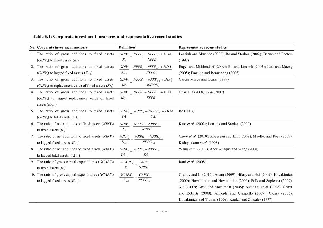
– 300 –
Table 5.1: Corporate investment measures and representative recent studies
No. Corporate investment measure Definitiona Representative recent studies
1. The ratio of gross additions to fixed assets (GINVt) to fixed assets (Kt) t
ttt
t
t
NPPEDDANPPENPPE
KGINV
1 Lensink and Murinde (2006); Bo and Sterken (2002); Barran and Peeters (1998)
2. The ratio of gross additions to fixed assets (GINVt) to lagged fixed assets (Kt–1) 1
1
1
t
ttt
t
t
NPPEDDANPPENPPE
KGINV Engel and Middendorf (2009); Bo and Lensink (2005); Koo and Maeng
(2005); Pawlina and Renneboog (2005)
3. The ratio of gross additions to fixed assets (GINVt) to replacement value of fixed assets (Krt) t
ttt
t
t
RNPPEDDANPPENPPE
KrGINV
1
Garcia-Marco and Ocana (1999)
4. The ratio of gross additions to fixed assets (GINVt) to lagged replacement value of fixed assets (Krt–1)
1
1
1
t
ttt
t
t
RPPEDDANPPENPPE
KrGINV Guariglia (2008); Gan (2007)
5. The ratio of gross additions to fixed assets (GINVt) to total assets (TAt) t
ttt
t
t
TADDANPPENPPE
TAGINV
1 Bo (2007)
6. The ratio of net additions to fixed assets (NINVt) to fixed assets (Kt) t
tt
t
t
NPPENPPENPPE
KNINV 1
Kato et al. (2002); Lensink and Sterken (2000)
7. The ratio of net additions to fixed assets (NINVt) to lagged fixed assets (Kt–1) 1
1
1
t
tt
t
t
NPPENPPENPPE
KNINV
Chow et al. (2010); Rousseau and Kim (2008); Mueller and Peev (2007); Kadapakkam et al. (1998)
8. The ratio of net additions to fixed assets (NINVt) to lagged total assets (TAt–1) 1
1
1
t
tt
t
t
TANPPENPPE
TANINV
Wang et al. (2009); Abdul-Haque and Wang (2008)
9. The ratio of gross capital expenditures (GCAPXt) to fixed assets (Kt) t
t
t
t
NPPECAPX
KGCAPX
Ratti et al. (2008)
10. The ratio of gross capital expenditures (GCAPXt) to lagged fixed assets (Kt–1) 11
t
t
t
t
NPPECAPX
KGCAPX Grundy and Li (2010); Adam (2009); Hilary and Hui (2009); Hovakimian
(2009); Hovakimian and Hovakimian (2009); Polk and Sapienza (2009); Xie (2009); Agca and Mozumdar (2008); Ascioglu et al. (2008); Chava and Roberts (2008); Almeida and Campello (2007); Cleary (2006); Hovakimian and Titman (2006); Kaplan and Zingales (1997)
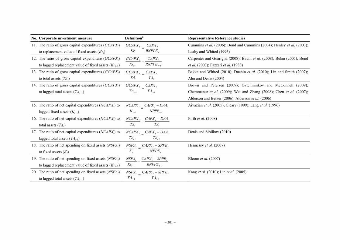
– 301 –
No. Corporate investment measure Definitiona Representative Reference studies
11. The ratio of gross capital expenditures (GCAPXt) to replacement value of fixed assets (Krt) t
t
t
t
RNPPECAPX
KrGCAPX
Cummins et al. (2006); Bond and Cummins (2004); Henley et al. (2003); Leahy and Whited (1996)
12. The ratio of gross capital expenditure (GCAPXt) to lagged replacement value of fixed assets (Krt–1) 11
t
t
t
t
RNPPECAPX
KrGCAPX
Carpenter and Guariglia (2008); Baum et al. (2008); Bulan (2005); Bond et al. (2003); Fazzari et al. (1988)
13. The ratio of gross capital expenditures (GCAPXt) to total assets (TAt) t
t
t
t
TACAPX
TAGCAPX
Bakke and Whited (2010); Duchin et al. (2010); Lin and Smith (2007); Ahn and Denis (2004)
14. The ratio of gross capital expenditures (GCAPXt) to lagged total assets (TAt–1) 11
t
t
t
t
TACAPX
TAGCAPX Brown and Petersen (2009); Ovtchinnikov and McConnell (2009);
Chemmanur et al. (2009); Wei and Zhang (2008); Chen et al. (2007); Alderson and Betker (2006); Alderson et al. (2006)
15. The ratio of net capital expenditures (NCAPXt) to lagged fixed assets (Kt–1) 11
t
tt
t
t
NPPEDAACAPX
KNCAPX
Aivazian et al. (2005); Cleary (1999); Lang et al. (1996)
16. The ratio of net capital expenditures (NCAPXt) to total assets (TAt) t
tt
t
t
TADAACAPX
TANCAPX
Firth et al. (2008)
17. The ratio of net capital expenditures (NCAPXt) to lagged total assets (TAt-1) 11
t
tt
t
t
TADAACAPX
TANCAPX
Denis and Sibilkov (2010)
18. The ratio of net spending on fixed assets (NSFAt) to fixed assets (Kt) t
tt
t
t
NPPESPPECAPX
KNSFA
Hennessy et al. (2007)
19. The ratio of net spending on fixed assets (NSFAt) to lagged replacement value of fixed assets (Krt–1) 11
t
tt
t
t
RNPPESPPECAPX
KrNSFA Bloom et al. (2007)
20. The ratio of net spending on fixed assets (NSFAt) to lagged total assets (TAt–1) 11
t
tt
t
t
TASPPECAPX
TANSFA
Kang et al. (2010); Lin et al. (2005)
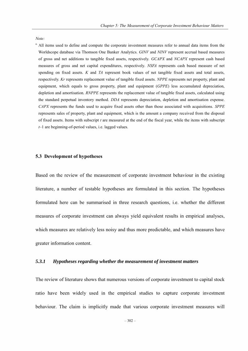
Chapter 5: The Measurement of Corporate Investment Behaviour Matters
– 302 –
Note: a. All items used to define and compute the corporate investment measures refer to annual data items from the
Worldscope database via Thomson One Banker Analytics. GINV and NINV represent accrual based measures of gross and net additions to tangible fixed assets, respectively. GCAPX and NCAPX represent cash based measures of gross and net capital expenditures, respectively. NSFA represents cash based measure of net spending on fixed assets. K and TA represent book values of net tangible fixed assets and total assets, respectively. Kr represents replacement value of tangible fixed assets. NPPE represents net property, plant and equipment, which equals to gross property, plant and equipment (GPPE) less accumulated depreciation, depletion and amortisation. RNPPE represents the replacement value of tangible fixed assets, calculated using the standard perpetual inventory method. DDA represents depreciation, depletion and amortisation expense. CAPX represents the funds used to acquire fixed assets other than those associated with acquisitions. SPPE represents sales of property, plant and equipment, which is the amount a company received from the disposal of fixed assets. Items with subscript t are measured at the end of the fiscal year, while the items with subscript t–1 are beginning-of-period values, i.e. lagged values.
5.3 Development of hypotheses
Based on the review of the measurement of corporate investment behaviour in the existing
literature, a number of testable hypotheses are formulated in this section. The hypotheses
formulated here can be summarised in three research questions, i.e. whether the different
measures of corporate investment can always yield equivalent results in empirical analyses,
which measures are relatively less noisy and thus more predictable, and which measures have
greater information content.
5.3.1 Hypotheses regarding whether the measurement of investment matters
The review of literature shows that numerous versions of corporate investment to capital stock
ratio have been widely used in the empirical studies to capture corporate investment
behaviour. The claim is implicitly made that various corporate investment measures will

Chapter 5: The Measurement of Corporate Investment Behaviour Matters
– 303 –
always yield equivalent empirical results. In other words, it is assumed that these corporate
investment measures can be used interchangeably without altering the conclusions drawn
from empirical analyses. However, we argue that, because different accounting principles are
involved in the calculation of relevant accounting figures, accrual based measures of
corporate investment may contain information about a company’s investment activities which
is not present in their cash based counterparts, and vice versa. Meanwhile, gross investment
measures and net investment measures are also likely to provide different information about
companies’ future productive capacity. Thus, the first hypothesis (Hypothesis 1) is formulated
as follows:
HN: Conclusions drawn from empirical analyses are not sensitive to the choice of
corporate investment measures;
HA: Conclusions drawn from empirical analyses are sensitive to the choice of
corporate investment measures.50
Hypothesis 1 can be tested by examining the pair-wise correlation coefficients among
the alternative corporate investment measures. The correlation coefficients can quantify the
amount of overlapping information contained in the alternatives. The correlation coefficient
analysis results are presented in Section 5.4. In addition, to better illustrate the extent to which
the choice of corporate investment measures may affect conclusions drawn from empirical
analyses, a conventional Tobin’s Q model is repeatedly estimated in Section 5.5 using
50 HN and HA represent the null hypothesis and alternative hypothesis, respectively.
Chapter 5: The Measurement of Corporate Investment Behaviour Matters
– 304 –
different measures of corporate investment as the dependent variable in their respective
regressions. The differences in the estimation results across regressions are expected to show
whether the measurement of corporate investment behaviour matters in empirical analyses.
5.3.2 Hypotheses regarding the volatility of investment measures
As discussed in Section 5.2, there is a potential timing difference in recognising capital
investment between accrual basis and cash basis accounting methods. Specifically, capital
investment is recognised when it is incurred under accrual basis accounting, whereas it is
recognised when cash is paid under cash basis accounting. Thus, cash based corporate
investment measures are subject to timing and mismatching problems which may cause them
to be noisy and unpredictable. By contrast, accrual based corporate investment to capital stock
ratios, which are supposed to mitigate the timing and mismatching problems of cash based
accounting figures, can be considered as smoothed measures of corporate investment
behaviour. Accordingly, the second hypothesis (Hypothesis 2) is formulated as follows:
HN: Cash based corporate investment measures are as noisy as their accrual based
counterparts;
HA: Cash based corporate investment measures are noisier than their accrual based
counterparts.
In addition, gross corporate investment measures are likely to behave differently from
net corporate investment measures, since the former focus on the overall investment in capital
Chapter 5: The Measurement of Corporate Investment Behaviour Matters
– 305 –
stock made by a company over certain period, whereas the latter further take depreciated
capital goods into consideration by subtracting depreciation expense charged for the same
period from the overall spending on capital stock. Because net corporate investment measures
are jointly determined by gross investment spending and depreciation expense, they are
expected to exhibit greater volatility than gross corporate investment measures. Therefore, it
is reasonable to expect that gross corporate investment measures are relatively less noisy and
more predictable than net corporate investment measures, especially when the managers have
an incentive to opportunistically manipulate depreciation figures. Accordingly, the third
hypothesis (Hypothesis 3) can be formulated as follows:
HN: Net corporate investment measures are as noisy as their corresponding gross
corporate investment measures;
HA: Net corporate investment measures are noisier than their corresponding gross
corporate investment measures.
Hypotheses 2 and 3 regarding the volatility (or predictability) of the corporate
investment measures are empirically tested in Section 5.6 using trend analysis.
5.3.3 Hypotheses regarding the information content of investment measures
Although the cash based measures are expected to contain more noise than their accrual based
counterparts, the proponents of cash flow basis accounting believe that cash flow measures
are less subject to distortions from differing accounting practices and managers opportunistic
manipulation, and thus impart such additional information that is not contained in the accrual

Chapter 5: The Measurement of Corporate Investment Behaviour Matters
– 306 –
based measures (see, for example, Salmi et al., 1990). Therefore, the fourth hypothesis
(Hypothesis 4) is developed as follows:
HN: Cash based corporate investment measures are as informative as their accrual
based counterparts;
HA: Cash based corporate investment measures are more informative than their accrual
based counterparts.
Meanwhile, it is also believed that net corporate investment measures contain more
information about a company’s future prospects than do gross corporate investment measures.
It is argued that gross investment includes both new investments and replacement investments.
New investments are undertaken to increase the scope of a company’s operations, while
replacement investments are made to maintain a company’s current operations. Since new
investments in additional operating capacity are expected to have a more significant effect on
the company’s future earnings, net corporate investment measures are likely to provide more
forward-looking information about company value and thus shareholders’ wealth.
Accordingly, the fifth hypothesis (Hypothesis 5) can be formulated as follows:
HN: Net corporate investment measures are as informative as their corresponding gross
corporate investment measures;
HA: Net corporate investment measures are more informative than their corresponding
gross corporate investment measures.
Hypotheses 4 and 5 regarding the information content of the corporate investment
Chapter 5: The Measurement of Corporate Investment Behaviour Matters
– 307 –
measures are tested in Section 5.7. Given the argument that changes in a company’s corporate
investment yield information about changes in the company’s future earnings that is not
captured by unexpected earnings (see, for example, Kerstein and Kim, 1995; and Park and
Pincus, 2003), we focus on the value relevant information content provided by the alternative
corporate investment measures.
5.4 Data and preliminary analysis
5.4.1 Data and measurement
The data are collected from the Worldscope database via Thomson One Banker Analytics. The
initial sample includes all companies listed on the London Stock Exchange (LSE), during the
period 1999–2008. We then discard utilities (SIC code 4900–4949), and financial companies
(SIC code 6000–6999), as these two industries are highly regulated. Companies that do not
have complete records of key data, such as net property, plant and equipment (NPPE), gross
property, plant and equipment (GPPE), total assets (TA), depreciation, depletion and
amortisation (DDA), capital expenditure (CAPX), and sales of property, plant and equipment
(SPPE), are dropped from our sample. A strongly balanced panel of company-level data over
the period from 1999 to 2008 is formed with 4,320 company-year observations. The balanced
panel dataset is preferred because it eliminates the potential effect of missing values on our
empirical results, allowing us to focus on our research question of whether the measurement
of corporate investment matters. The twenty alternative measures of corporate investment

Chapter 5: The Measurement of Corporate Investment Behaviour Matters
– 308 –
identified in the existing literature (see Table 5.1 for detailed definitions) are calculated using
the data from the panel of UK-listed companies over the period 1999–2008.
5.4.2 Summary statistics
The summary statistics of the alternative measures of corporate investment are presented in
Table 5.2. In addition to the conventional statistics, we also calculated the coefficient of
variation (CV) for each of the corporate investment measures. The coefficient of variation is
defined as the ratio of the standard deviation to the absolute mean of the underlying variable.
Thus, it is a dimensionless statistic which can be used to compare volatility among variables
with widely different means. As is evident in Panel A, extreme values appear in almost all the
corporate investment to capital stock ratios, indicating that the observed corporate investment
measures are severely distorted by outliers which may have a significant effect upon the
results of our empirical tests. In order to reduce the potential impact of outliers, the observed
corporate investment measures are winsorised at both the top and bottom 5th percentiles.
Specifically, for all of the investment ratios, the extreme values, which are defined as the top
and bottom 5 percent of the sample observations, are assigned to the cut-off values. This
approach not only reduces the potential impact of outliers but also allows the full use of
observations. Given the argument that winsorisation estimators are expected to be more
plausible and robust than those of the standard transformations such as trimming (Baum et al,
2008; and Chay and Suh, 2009), the empirical results presented in this chapter are obtained
based on the observations that are winsorised at both the top and bottom 5th percentiles.
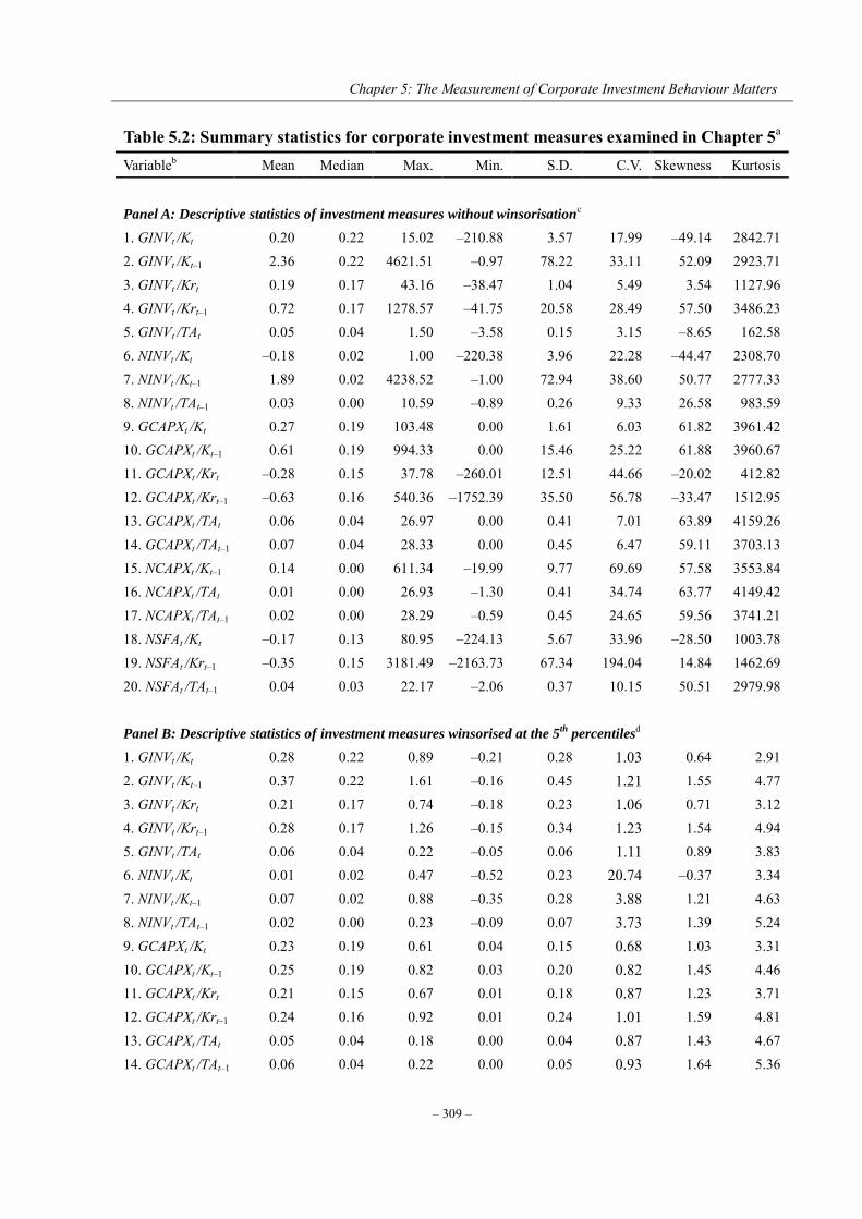
Chapter 5: The Measurement of Corporate Investment Behaviour Matters
– 309 –
Table 5.2: Summary statistics for corporate investment measures examined in Chapter 5a Variableb Mean Median Max. Min. S.D. C.V. Skewness Kurtosis
Panel A: Descriptive statistics of investment measures without winsorisation
c 1. GINVt /Kt 0.20 0.22 15.02 –210.88 3.57 17.99 –49.14 2842.71 2. GINVt /Kt–1 2.36 0.22 4621.51 –0.97 78.22 33.11 52.09 2923.71 3. GINVt /Krt 0.19 0.17 43.16 –38.47 1.04 5.49 3.54 1127.96 4. GINVt /Krt–1 0.72 0.17 1278.57 –41.75 20.58 28.49 57.50 3486.23 5. GINVt /TAt 0.05 0.04 1.50 –3.58 0.15 3.15 –8.65 162.58 6. NINVt /Kt –0.18 0.02 1.00 –220.38 3.96 22.28 –44.47 2308.70 7. NINVt /Kt–1 1.89 0.02 4238.52 –1.00 72.94 38.60 50.77 2777.33 8. NINVt /TAt–1 0.03 0.00 10.59 –0.89 0.26 9.33 26.58 983.59 9. GCAPXt /Kt 0.27 0.19 103.48 0.00 1.61 6.03 61.82 3961.42 10. GCAPXt /Kt–1 0.61 0.19 994.33 0.00 15.46 25.22 61.88 3960.67 11. GCAPXt /Krt –0.28 0.15 37.78 –260.01 12.51 44.66 –20.02 412.82 12. GCAPXt /Krt–1 –0.63 0.16 540.36 –1752.39 35.50 56.78 –33.47 1512.95 13. GCAPXt /TAt 0.06 0.04 26.97 0.00 0.41 7.01 63.89 4159.26 14. GCAPXt /TAt–1 0.07 0.04 28.33 0.00 0.45 6.47 59.11 3703.13 15. NCAPXt /Kt–1 0.14 0.00 611.34 –19.99 9.77 69.69 57.58 3553.84 16. NCAPXt /TAt 0.01 0.00 26.93 –1.30 0.41 34.74 63.77 4149.42 17. NCAPXt /TAt–1 0.02 0.00 28.29 –0.59 0.45 24.65 59.56 3741.21 18. NSFAt /Kt –0.17 0.13 80.95 –224.13 5.67 33.96 –28.50 1003.78 19. NSFAt /Krt–1 –0.35 0.15 3181.49 –2163.73 67.34 194.04 14.84 1462.69 20. NSFAt /TAt–1 0.04 0.03 22.17 –2.06 0.37 10.15 50.51 2979.98 Panel B: Descriptive statistics of investment measures winsorised at the 5
th percentiles
d 1. GINVt /Kt 0.28 0.22 0.89 –0.21 0.28 1.03 0.64 2.91 2. GINVt /Kt–1 0.37 0.22 1.61 –0.16 0.45 1.21 1.55 4.77 3. GINVt /Krt 0.21 0.17 0.74 –0.18 0.23 1.06 0.71 3.12 4. GINVt /Krt–1 0.28 0.17 1.26 –0.15 0.34 1.23 1.54 4.94 5. GINVt /TAt 0.06 0.04 0.22 –0.05 0.06 1.11 0.89 3.83 6. NINVt /Kt 0.01 0.02 0.47 –0.52 0.23 20.74 –0.37 3.34 7. NINVt /Kt–1 0.07 0.02 0.88 –0.35 0.28 3.88 1.21 4.63 8. NINVt /TAt–1 0.02 0.00 0.23 –0.09 0.07 3.73 1.39 5.24 9. GCAPXt /Kt 0.23 0.19 0.61 0.04 0.15 0.68 1.03 3.31 10. GCAPXt /Kt–1 0.25 0.19 0.82 0.03 0.20 0.82 1.45 4.46 11. GCAPXt /Krt 0.21 0.15 0.67 0.01 0.18 0.87 1.23 3.71 12. GCAPXt /Krt–1 0.24 0.16 0.92 0.01 0.24 1.01 1.59 4.81 13. GCAPXt /TAt 0.05 0.04 0.18 0.00 0.04 0.87 1.43 4.67 14. GCAPXt /TAt–1 0.06 0.04 0.22 0.00 0.05 0.93 1.64 5.36
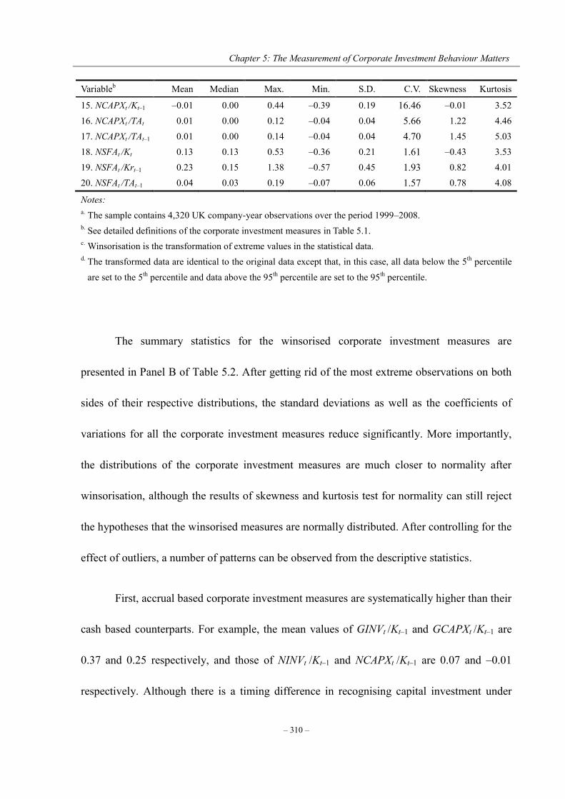
Chapter 5: The Measurement of Corporate Investment Behaviour Matters
– 310 –
Variableb Mean Median Max. Min. S.D. C.V. Skewness Kurtosis
15. NCAPXt /Kt–1 –0.01 0.00 0.44 –0.39 0.19 16.46 –0.01 3.52 16. NCAPXt /TAt 0.01 0.00 0.12 –0.04 0.04 5.66 1.22 4.46 17. NCAPXt /TAt–1 0.01 0.00 0.14 –0.04 0.04 4.70 1.45 5.03 18. NSFAt /Kt 0.13 0.13 0.53 –0.36 0.21 1.61 –0.43 3.53 19. NSFAt /Krt–1 0.23 0.15 1.38 –0.57 0.45 1.93 0.82 4.01 20. NSFAt /TAt–1 0.04 0.03 0.19 –0.07 0.06 1.57 0.78 4.08
Notes: a. The sample contains 4,320 UK company-year observations over the period 1999–2008. b. See detailed definitions of the corporate investment measures in Table 5.1. c. Winsorisation is the transformation of extreme values in the statistical data. d. The transformed data are identical to the original data except that, in this case, all data below the 5th percentile
are set to the 5th percentile and data above the 95th percentile are set to the 95th percentile.
The summary statistics for the winsorised corporate investment measures are
presented in Panel B of Table 5.2. After getting rid of the most extreme observations on both
sides of their respective distributions, the standard deviations as well as the coefficients of
variations for all the corporate investment measures reduce significantly. More importantly,
the distributions of the corporate investment measures are much closer to normality after
winsorisation, although the results of skewness and kurtosis test for normality can still reject
the hypotheses that the winsorised measures are normally distributed. After controlling for the
effect of outliers, a number of patterns can be observed from the descriptive statistics.
First, accrual based corporate investment measures are systematically higher than their
cash based counterparts. For example, the mean values of GINVt /Kt–1 and GCAPXt /Kt–1 are
0.37 and 0.25 respectively, and those of NINVt /Kt–1 and NCAPXt /Kt–1 are 0.07 and –0.01
respectively. Although there is a timing difference in recognising capital investment under
Chapter 5: The Measurement of Corporate Investment Behaviour Matters
– 311 –
different accounting methods, the timing difference cannot adequately justify the large gap
between the mean values of accrual based and cash based investment measures. The
differences between accrual based and cash based investment measures are largely due to
asset revaluations as well as assets associated with acquisitions, which are reflected in the
carrying amount of tangible fixed assets on balance sheet but cannot be captured by capital
expenditures on cash flow statement. In addition, the coefficients of variation suggest that, on
average, cash flow based investment measures are less volatile that their accrual based
counterparts. For example, the coefficients of variation of GINVt /Kt and GCAPXt /Kt are 1.03
and 0.68 respectively, and those of GINVt /Krt and GCAPXt /Krt are 1.06 and 0.87 respectively.
It is worth noting that the extremely high levels of volatility of NINVt /Kt, NCAPXt /Kt–1 and
NCAPXt /TAt, as suggested by their respective coefficients of variation, are likely to be caused
by their low mean values, which are close to zero. It is acknowledged that, when the mean
value is close to zero, the coefficient of variation is highly sensitive to small changes in the
mean, limiting its usefulness.
Second, it is evident that the mean values of gross corporate investment measures are
systematically higher than those of their corresponding net corporate investment measures.
For example, the mean value of GINVt /Kt is 0.28, while that of NINVt /Kt is 0.01; the mean
values of GCAPXt /Kt–1 and NCAPXt /Kt–1 are 0.25 and –0.01, respectively. The difference in
the mean values of gross and net investment measures is directly related to their respective
definitions. Deducting depreciation expense from overall investment creates a large wedge

Chapter 5: The Measurement of Corporate Investment Behaviour Matters
– 312 –
between the mean values of gross investment measures and those of net investment measures.
Meanwhile, as expected, gross investment measures are less volatile than net investment
measures, as indicated by the coefficients of variation. However, the higher values of the
coefficient of variation for the net investment measures may also be attributable to their lower
mean values.
Third, the use of lagged proxies of capital stock to scale investment spending inflates
the values of corporate investment measures significantly. After lagging the proxy for capital
stock by one period, the mean of gross investment to fixed assets ratio (GINV/K) increases
from 0.28 to 0.37 and the mean of gross investment to replacement value of fixed assets ratio
(GINV/Kr) increases from 0.21 to 0.28. Meanwhile, the volatilities of the corporate investment
measures are also likely to be inflated by lagging the proxy for capital stock. For example, the
coefficients of variation of GINVt /Kt and GINVt /Kt–1 are 1.03 and 1.21 respectively, and those
of GINVt /Kr and GINVt /Kr–1 are 1.06 and 1.23 respectively.
In addition, the choice of the proxies for capital stock influences the mean values of
the corporate investment measures substantially. In general, corporate investment measures
scaled by the replacement value of fixed assets are lower than those scaled by the book value
of fixed assets, implying that changes in price level have a substantial impact on the value of
capital goods, while the corporate investment measures scaled by book value of total assets
typically have the lowest means values among the alternatives.
Chapter 5: The Measurement of Corporate Investment Behaviour Matters
– 313 –
The observed differences in the mean values of the corporate investment measures are
formally tested using mean-comparison tests. The results of the pair-wise t tests on the
equality of means are reported in Appendix 5.B. The null hypothesis that the means of the
corresponding corporate investment measures are equal can be firmly rejected in almost all
instances. In addition, the annual mean value of each corporate investment measure is plotted
over time in Appendix 5.C, providing a visual comparison among the alternative measures of
corporate investment.
5.4.3 Correlation coefficient analysis
To gauge the extent of correlation among the twenty measures of corporate investment, we
compute correlation coefficients between each pair of them. A number of distinct patterns can
be observed from the Pearson correlation coefficients presented in Table 5.3.
First, the correlation coefficients reveal a considerable degree of association between
each pair of corporate investment measures with only five exceptions. Most of the correlation
coefficients are significantly positive at the 1% significance level, suggesting that, although
the corporate investment measures are specified differently, they do provide similar
information about a company’s investing activities. However, it is also found that the
correlation coefficients among the corporate investment measures are not uniformly positively.
Seven pairs of corporate investment measures are found to be negatively correlated with each
other, which appears surprising given that all the measures are supposed to depict the
Chapter 5: The Measurement of Corporate Investment Behaviour Matters
– 314 –
investment behaviour of the same batch of companies over the same period of time.
Specifically, the correlation coefficient matrix shows that GINVt /Kt is negatively correlated
with GCAPXt /TAt, NCAPXt /Kt–1, NCAPXt /TAt and NCAPXt /TAt–1, while NCAPXt /Kt–1 is
negatively correlated with GINVt /Kt–1, GINVt /Krt and GINVt /Krt–1. The negative correlation
coefficients vary between –0.03 and –0.31. Four of them are statistically significant at the 1%
significance level, and the others are also marginally significant. The strongest negative
correlation is observed between GINVt /Kt and NCAPXt /Kt–1. The correlation coefficient of
–0.31 suggests that the negative assocation between the two corporate investment measures is
not only statistically significant but also economically significant. If these two significantly
and negatively correlated corporate investment measures are used to investigate the same
research question, they are likely to yield qualitatively dissimilar results. Since the negative
correlations are only observed between accrual based and cash based corporate investment
measures, it is plausible to argue that the differences among alternative measures are
primarily attributable to the different accounting principles involved in the preparation of
relevant accounting figures.
Second, a significant definitional correlation effect can be observed from the
correlation coefficient matrix. In other words, corporate investment measures which are
similarly specified are likely to be highly correlated with each other. For example, the highest
correlation coefficients are observed between GINVt /Kt and GINVt /Kt–1, GINVt /Krt and
GINVt /Krt–1, NINVt /Kt and NINVt /Kt–1, GCAPXt /Kt and GCAPXt /Kt–1, GCAPXt /Krt and
Chapter 5: The Measurement of Corporate Investment Behaviour Matters
– 315 –
GCAPXt /Krt–1, GCAPXt /TAt and GCAPXt /TAt–1, and NCAPXt /TAt and NCAPXt /TAt–1,
ranging from 0.85 to 0.96. These significant associations also suggest that lagging the proxy
for capital stock by one period does not create many changes in the behaviour of corporate
investment measures. Therefore, the empirical results of corporate investment research are
unlikely to be affected by different assumptions regarding the specific time point at which the
investment decisions are made. Moreover, the correlation coefficients between GINVt /Kt and
GINVt /Krt, GINVt /Kt–1 and GINVt /Krt–1, GCAPXt /Kt and GCAPXt /Krt, and GCAPXt /Kt–1 and
GCAPXt /Krt–1 are 0.81, 0.81, 0.62 and 0.72, respectively, suggesting that the choice between
using book value or replacement value of capital stock to deflate corporate investment is also
unlikely to have significant influence upon the results of empirical analyses.
Third, the weakest pair-wise correlations are found between corporate investment
measures which are constructed in completely different ways. The correlation coefficient
between GINVt /Kt–1 and GCAPXt /TAt, for example, is as low as 0.005 and is not significantly
different from zero. The independence of the two corporate investment measures is likely to
be caused by the differences in measuring both investment spending and capital stock, which
leads to less overlapping information being conveyed by the two variables. Overall, the
correlation coefficients represented in Table 5.3 suggest that the conflicting results observed
in the existing literature may, at least partially, be attributable to the choice of corporate
investment measures.
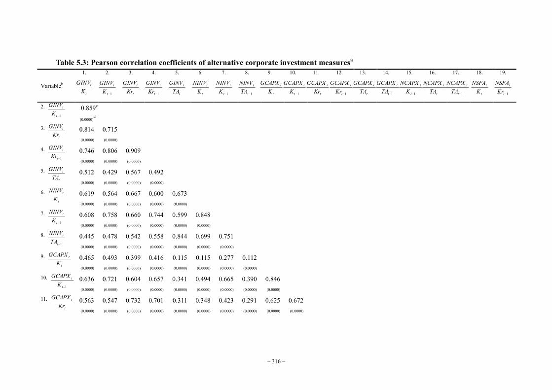
– 316 –
Table 5.3: Pearson correlation coefficients of alternative corporate investment measuresa
Variableb
1.
t
t
KGINV
2.
1t
t
KGINV
3.
t
t
KrGINV
4.
1t
t
KrGINV
5.
t
t
TAGINV
6.
t
t
KNINV
7.
1t
t
KNINV
8.
1t
t
TANINV
9.
t
t
KGCAPX
10.
1t
t
KGCAPX
11.
t
t
KrGCAPX
12.
1t
t
KrGCAPX
13.
t
t
TAGCAPX
14.
1t
t
TAGCAPX
15.
1t
t
KNCAPX
16.
t
t
TANCAPX
17.
1t
t
TANCAPX
18.
t
t
KNSFA
19.
1t
t
KrNSFA
2. 1t
t
KGINV
0.859c (0.0000)
d
3.
t
t
KrGINV
0.814 (0.0000)
0.715 (0.0000)
4. 1t
t
KrGINV
0.746 (0.0000)
0.806 (0.0000)
0.909 (0.0000)
5. t
t
TAGINV
0.512 (0.0000)
0.429 (0.0000)
0.567 (0.0000)
0.492 (0.0000)
6. t
t
KNINV
0.619 (0.0000)
0.564 (0.0000)
0.667 (0.0000)
0.600 (0.0000)
0.673 (0.0000)
7. 1t
t
KNINV
0.608 (0.0000)
0.758 (0.0000)
0.660 (0.0000)
0.744 (0.0000)
0.599 (0.0000)
0.848 (0.0000)
8. 1t
t
TANINV
0.445 (0.0000)
0.478 (0.0000)
0.542 (0.0000)
0.558 (0.0000)
0.844 (0.0000)
0.699 (0.0000)
0.751 (0.0000)
9. t
t
KGCAPX
0.465 (0.0000)
0.493 (0.0000)
0.399 (0.0000)
0.416 (0.0000)
0.115 (0.0000)
0.115 (0.0000)
0.277 (0.0000)
0.112 (0.0000)
10. 1t
t
KGCAPX
0.636 (0.0000)
0.721 (0.0000)
0.604 (0.0000)
0.657 (0.0000)
0.341 (0.0000)
0.494 (0.0000)
0.665 (0.0000)
0.390 (0.0000)
0.846 (0.0000)
11. t
t
KrGCAPX
0.563 (0.0000)
0.547 (0.0000)
0.732 (0.0000)
0.701 (0.0000)
0.311 (0.0000)
0.348 (0.0000)
0.423 (0.0000)
0.291 (0.0000)
0.625 (0.0000)
0.672 (0.0000)
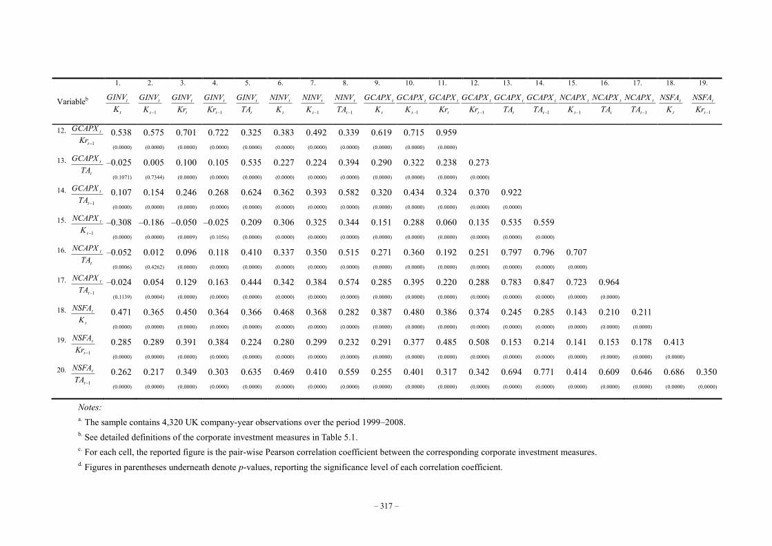
– 317 –
Variableb
1.
t
t
KGINV
2.
1t
t
KGINV
3.
t
t
KrGINV
4.
1t
t
KrGINV
5.
t
t
TAGINV
6.
t
t
KNINV
7.
1t
t
KNINV
8.
1t
t
TANINV
9.
t
t
KGCAPX
10.
1t
t
KGCAPX
11.
t
t
KrGCAPX
12.
1t
t
KrGCAPX
13.
t
t
TAGCAPX
14.
1t
t
TAGCAPX
15.
1t
t
KNCAPX
16.
t
t
TANCAPX
17.
1t
t
TANCAPX
18.
t
t
KNSFA
19.
1t
t
KrNSFA
12. 1t
t
KrGCAPX
0.538 (0.0000)
0.575 (0.0000)
0.701 (0.0000)
0.722 (0.0000)
0.325 (0.0000)
0.383 (0.0000)
0.492 (0.0000)
0.339 (0.0000)
0.619 (0.0000)
0.715 (0.0000)
0.959 (0.0000)
13. t
t
TAGCAPX
–0.025 (0.1071)
0.005 (0.7344)
0.100 (0.0000)
0.105 (0.0000)
0.535 (0.0000)
0.227 (0.0000)
0.224 (0.0000)
0.394 (0.0000)
0.290 (0.0000)
0.322 (0.0000)
0.238 (0.0000)
0.273 (0.0000)
14. 1t
t
TAGCAPX
0.107 (0.0000)
0.154 (0.0000)
0.246 (0.0000)
0.268 (0.0000)
0.624 (0.0000)
0.362 (0.0000)
0.393 (0.0000)
0.582 (0.0000)
0.320 (0.0000)
0.434 (0.0000)
0.324 (0.0000)
0.370 (0.0000)
0.922 (0.0000)
15. 1t
t
KNCAPX
–0.308 (0.0000)
–0.186 (0.0000)
–0.050 (0.0009)
–0.025 (0.1056)
0.209 (0.0000)
0.306 (0.0000)
0.325 (0.0000)
0.344 (0.0000)
0.151 (0.0000)
0.288 (0.0000)
0.060 (0.0000)
0.135 (0.0000)
0.535 (0.0000)
0.559 (0.0000)
16. t
t
TANCAPX
–0.052 (0.0006)
0.012 (0.4262)
0.096 (0.0000)
0.118 (0.0000)
0.410 (0.0000)
0.337 (0.0000)
0.350 (0.0000)
0.515 (0.0000)
0.271 (0.0000)
0.360 (0.0000)
0.192 (0.0000)
0.251 (0.0000)
0.797 (0.0000)
0.796 (0.0000)
0.707 (0.0000)
17. 1t
t
TANCAPX
–0.024 (0.1139)
0.054 (0.0004)
0.129 (0.0000)
0.163 (0.0000)
0.444 (0.0000)
0.342 (0.0000)
0.384 (0.0000)
0.574 (0.0000)
0.285 (0.0000)
0.395 (0.0000)
0.220 (0.0000)
0.288 (0.0000)
0.783 (0.0000)
0.847 (0.0000)
0.723 (0.0000)
0.964 (0.0000)
18. t
t
KNSFA
0.471 (0.0000)
0.365 (0.0000)
0.450 (0.0000)
0.364 (0.0000)
0.366 (0.0000)
0.468 (0.0000)
0.368 (0.0000)
0.282 (0.0000)
0.387 (0.0000)
0.480 (0.0000)
0.386 (0.0000)
0.374 (0.0000)
0.245 (0.0000)
0.285 (0.0000)
0.143 (0.0000)
0.210 (0.0000)
0.211 (0.0000)
19. 1t
t
KrNSFA
0.285 (0.0000)
0.289 (0.0000)
0.391 (0.0000)
0.384 (0.0000)
0.224 (0.0000)
0.280 (0.0000)
0.299 (0.0000)
0.232 (0.0000)
0.291 (0.0000)
0.377 (0.0000)
0.485 (0.0000)
0.508 (0.0000)
0.153 (0.0000)
0.214 (0.0000)
0.141 (0.0000)
0.153 (0.0000)
0.178 (0.0000)
0.413 (0.0000)
20. 1t
t
TANSFA
0.262 (0.0000)
0.217 (0.0000)
0.349 (0.0000)
0.303 (0.0000)
0.635 (0.0000)
0.469 (0.0000)
0.410 (0.0000)
0.559 (0.0000)
0.255 (0.0000)
0.401 (0.0000)
0.317 (0.0000)
0.342 (0.0000)
0.694 (0.0000)
0.771 (0.0000)
0.414 (0.0000)
0.609 (0.0000)
0.646 (0.0000)
0.686 (0.0000)
0.350 (0.0000)
Notes: a. The sample contains 4,320 UK company-year observations over the period 1999–2008. b. See detailed definitions of the corporate investment measures in Table 5.1. c. For each cell, the reported figure is the pair-wise Pearson correlation coefficient between the corresponding corporate investment measures. d. Figures in parentheses underneath denote p-values, reporting the significance level of each correlation coefficient.
Chapter 5: The Measurement of Corporate Investment Behaviour Matters
– 318 –
Given the fact that the winsorised corporate investment measures are still skewed and
leptokurtotic, a nonparametric method, i.e. Spearman’s rank correlation, is also employed to
check the robustness of the association between each pair of corporate investment measures.
Spearman’s rank correlation assesses how well the relationship between a pair of corporate
investment measures can be described as a monotonic function. More specifically, this
method converts the values of the corporate investment measures into ranks, and evaluate
whether the orders ranked by different corporate investment measures are monotonically
related. Increasing positive values imply increasing agreement between the rankings
according to different corporate investment measures. Spearman’s rank correlation
coefficients are presented in Appendix 5.D. The associations among the corporate investment
measures observed from Table 5.3 are confirmed by the results of the nonparametric method,
except that the negative pair-wise correlations reduce to four and become less significant
when the assumption of normality are relaxed.
5.5 A simple regression of Tobin’s Q model of investment
Although our preliminary analysis reveals that most of the corporate investment measures are
positively correlated with one another, this does not necessarily imply that they will behave
similarly in empirical analyses. More importantly, negative pair-wise associations are also
found between some corporate investment measures. These negatively associated corporate
investment measures are likely to yield qualitatively dissimilar results in empirical analyses.
Therefore, the principal purpose of this section is to illustrate the extent to which the choice of
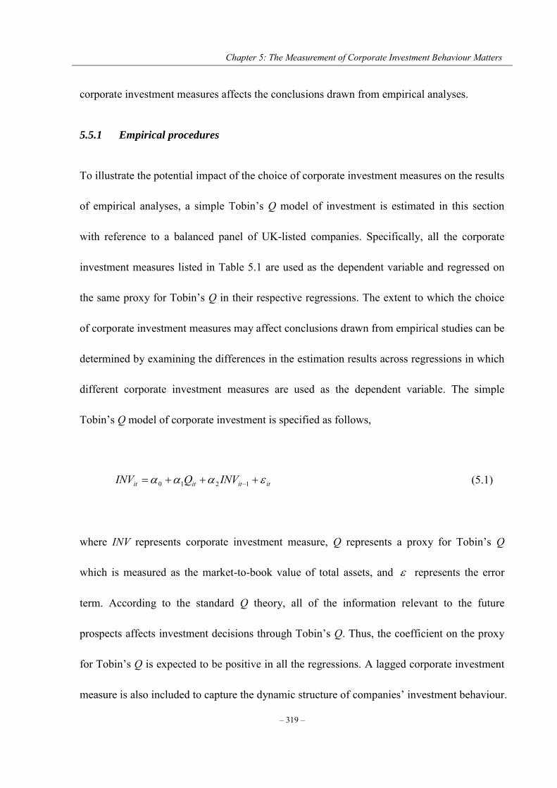
Chapter 5: The Measurement of Corporate Investment Behaviour Matters
– 319 –
corporate investment measures affects the conclusions drawn from empirical analyses.
5.5.1 Empirical procedures
To illustrate the potential impact of the choice of corporate investment measures on the results
of empirical analyses, a simple Tobin’s Q model of investment is estimated in this section
with reference to a balanced panel of UK-listed companies. Specifically, all the corporate
investment measures listed in Table 5.1 are used as the dependent variable and regressed on
the same proxy for Tobin’s Q in their respective regressions. The extent to which the choice
of corporate investment measures may affect conclusions drawn from empirical studies can be
determined by examining the differences in the estimation results across regressions in which
different corporate investment measures are used as the dependent variable. The simple
Tobin’s Q model of corporate investment is specified as follows,
itititit INVQINV 1210 (5.1)
where INV represents corporate investment measure, Q represents a proxy for Tobin’s Q
which is measured as the market-to-book value of total assets, and represents the error
term. According to the standard Q theory, all of the information relevant to the future
prospects affects investment decisions through Tobin’s Q. Thus, the coefficient on the proxy
for Tobin’s Q is expected to be positive in all the regressions. A lagged corporate investment
measure is also included to capture the dynamic structure of companies’ investment behaviour.

Chapter 5: The Measurement of Corporate Investment Behaviour Matters
– 320 –
Moreover, we control for time effects by adding year dummies. Equation 5.1 is estimated
repeatedly for different corporate investment measures, using system-GMM estimators.
5.5.2 Empirical results
The system-GMM estimation results for the simple Tobin’s Q model of corporate investment
are reported in Table 5.4. As expected, distinct conclusions with respect to the association
between Tobin’s Q and companies’ investment behaviour can be drawn when different
corporate investment measures are employed as the dependent variable.
More specifically, as shown in column 3 of Table 5.4, the coefficient on Tobin’s Q
turns out to be positive in 14 regressions, indicating that higher Q values encourage
companies to undertake more investment projects. However, the estimation results for the
remaining 6 regressions indicate the opposite that the Tobin’s Q affects corporate investment
adversely. When GINVt /Kt–1, GCAPXt /Kt, GCAPXt /Kt–1, GCAPXt /Krt–1, NSFAt /Kt and NSFAt
/Krt–1 are regressed on the proxy for Tobin’s Q, the estimation results suggest that the positive
association between corporate investment and Tobin’s Q is statistically significant, whereas,
when GINVt /TAt and NINVt /TAt–1 are regressed on the same proxy for Tobin’s Q, the
association between corporate investment and Tobin’s Q is also statistically significant but
negative. Therefore, it is shown that no consensus can be reached about either the sign or the
significance level of the relation between corporate investment behaviour and Tobin’s Q
across regressions where different measures of corporate investment are employed.
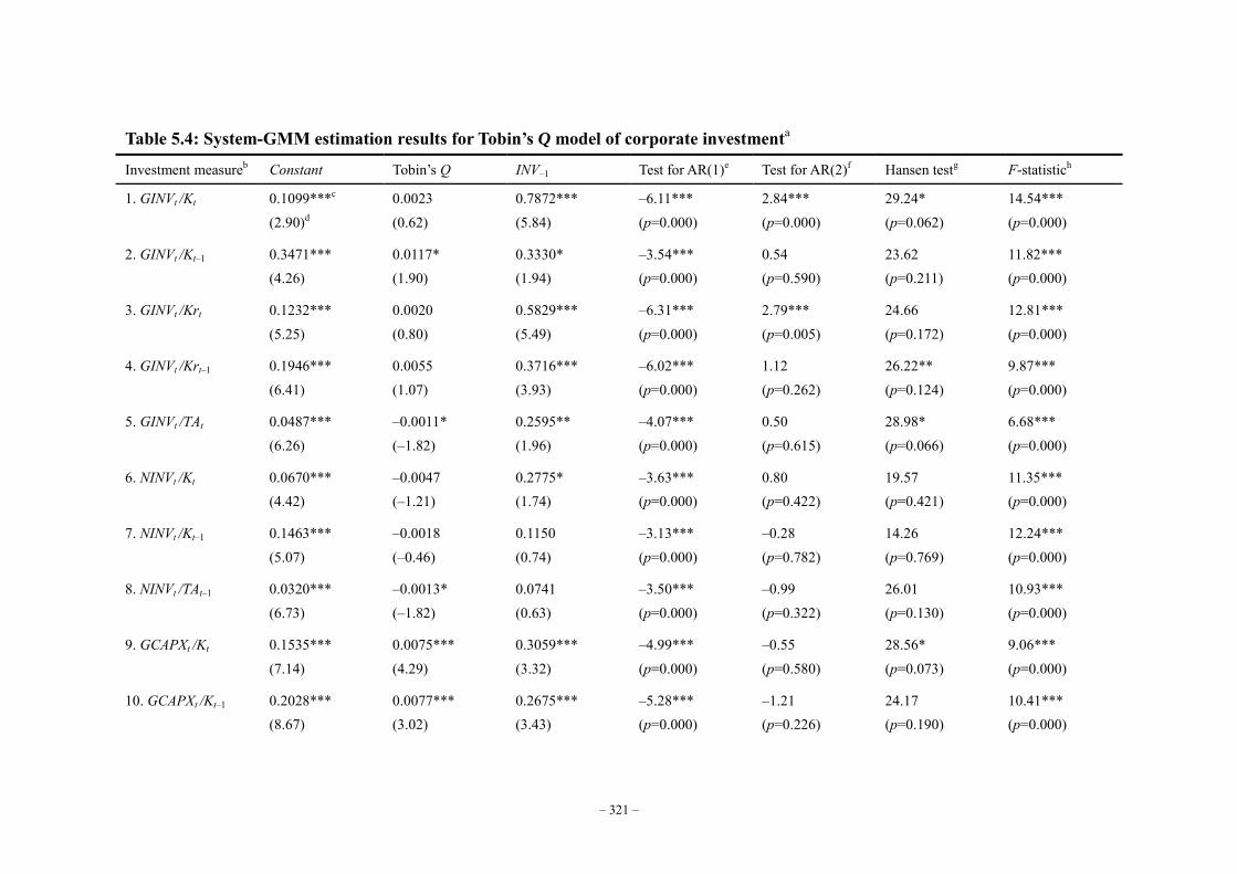
– 321 –
Table 5.4: System-GMM estimation results for Tobin’s Q model of corporate investmenta
Investment measureb Constant Tobin’s Q INV–1 Test for AR(1)e Test for AR(2)f Hansen testg F-statistich
1. GINVt /Kt 0.1099***c (2.90)d
0.0023 (0.62)
0.7872*** (5.84)
–6.11*** (p=0.000)
2.84*** (p=0.000)
29.24* (p=0.062)
14.54*** (p=0.000)
2. GINVt /Kt–1 0.3471*** (4.26)
0.0117* (1.90)
0.3330* (1.94)
–3.54*** (p=0.000)
0.54 (p=0.590)
23.62 (p=0.211)
11.82*** (p=0.000)
3. GINVt /Krt 0.1232*** (5.25)
0.0020 (0.80)
0.5829*** (5.49)
–6.31*** (p=0.000)
2.79*** (p=0.005)
24.66 (p=0.172)
12.81*** (p=0.000)
4. GINVt /Krt–1 0.1946*** (6.41)
0.0055 (1.07)
0.3716*** (3.93)
–6.02*** (p=0.000)
1.12 (p=0.262)
26.22** (p=0.124)
9.87*** (p=0.000)
5. GINVt /TAt 0.0487*** (6.26)
–0.0011* (–1.82)
0.2595** (1.96)
–4.07*** (p=0.000)
0.50 (p=0.615)
28.98* (p=0.066)
6.68*** (p=0.000)
6. NINVt /Kt 0.0670*** (4.42)
–0.0047 (–1.21)
0.2775* (1.74)
–3.63*** (p=0.000)
0.80 (p=0.422)
19.57 (p=0.421)
11.35*** (p=0.000)
7. NINVt /Kt–1 0.1463*** (5.07)
–0.0018 (–0.46)
0.1150 (0.74)
–3.13*** (p=0.000)
–0.28 (p=0.782)
14.26 (p=0.769)
12.24*** (p=0.000)
8. NINVt /TAt–1 0.0320*** (6.73)
–0.0013* (–1.82)
0.0741 (0.63)
–3.50*** (p=0.000)
–0.99 (p=0.322)
26.01 (p=0.130)
10.93*** (p=0.000)
9. GCAPXt /Kt 0.1535*** (7.14)
0.0075*** (4.29)
0.3059*** (3.32)
–4.99*** (p=0.000)
–0.55 (p=0.580)
28.56* (p=0.073)
9.06*** (p=0.000)
10. GCAPXt /Kt–1 0.2028*** (8.67)
0.0077*** (3.02)
0.2675*** (3.43)
–5.28*** (p=0.000)
–1.21 (p=0.226)
24.17 (p=0.190)
10.41*** (p=0.000)
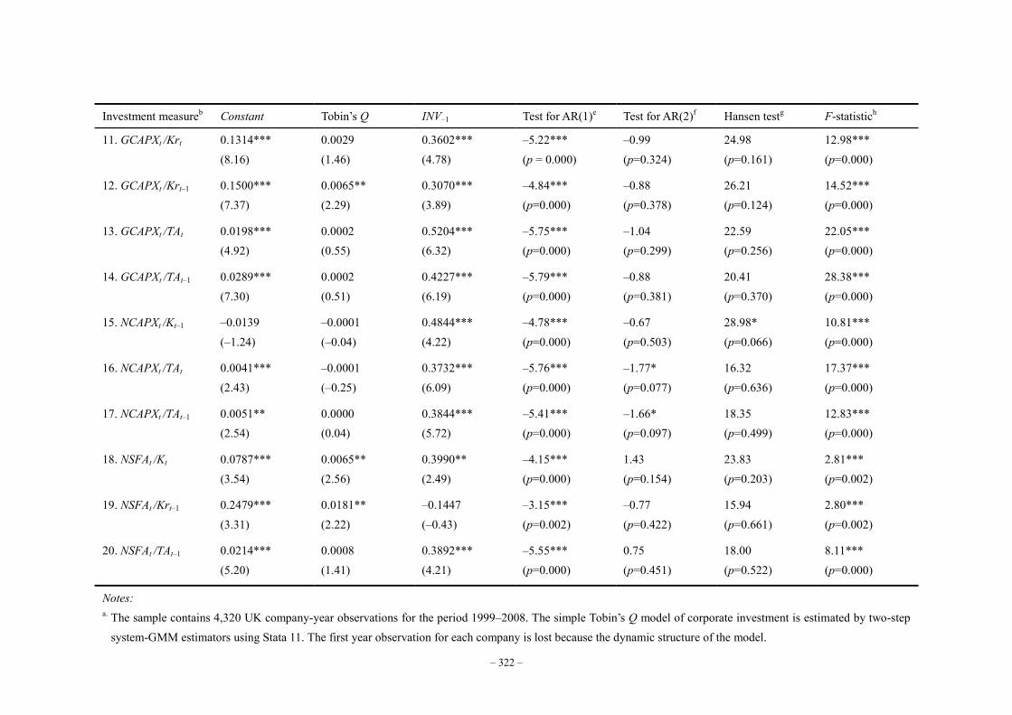
– 322 –
Investment measureb Constant Tobin’s Q INV–1 Test for AR(1)e Test for AR(2)f Hansen testg F-statistich
11. GCAPXt /Krt 0.1314*** (8.16)
0.0029 (1.46)
0.3602*** (4.78)
–5.22*** (p = 0.000)
–0.99 (p=0.324)
24.98 (p=0.161)
12.98*** (p=0.000)
12. GCAPXt /Krt–1 0.1500*** (7.37)
0.0065** (2.29)
0.3070*** (3.89)
–4.84*** (p=0.000)
–0.88 (p=0.378)
26.21 (p=0.124)
14.52*** (p=0.000)
13. GCAPXt /TAt 0.0198*** (4.92)
0.0002 (0.55)
0.5204*** (6.32)
–5.75*** (p=0.000)
–1.04 (p=0.299)
22.59 (p=0.256)
22.05*** (p=0.000)
14. GCAPXt /TAt–1 0.0289*** (7.30)
0.0002 (0.51)
0.4227*** (6.19)
–5.79*** (p=0.000)
–0.88 (p=0.381)
20.41 (p=0.370)
28.38*** (p=0.000)
15. NCAPXt /Kt–1 –0.0139 (–1.24)
–0.0001 (–0.04)
0.4844*** (4.22)
–4.78*** (p=0.000)
–0.67 (p=0.503)
28.98* (p=0.066)
10.81*** (p=0.000)
16. NCAPXt /TAt 0.0041*** (2.43)
–0.0001 (–0.25)
0.3732*** (6.09)
–5.76*** (p=0.000)
–1.77* (p=0.077)
16.32 (p=0.636)
17.37*** (p=0.000)
17. NCAPXt /TAt–1 0.0051** (2.54)
0.0000 (0.04)
0.3844*** (5.72)
–5.41*** (p=0.000)
–1.66* (p=0.097)
18.35 (p=0.499)
12.83*** (p=0.000)
18. NSFAt /Kt 0.0787*** (3.54)
0.0065** (2.56)
0.3990** (2.49)
–4.15*** (p=0.000)
1.43 (p=0.154)
23.83 (p=0.203)
2.81*** (p=0.002)
19. NSFAt /Krt–1 0.2479*** (3.31)
0.0181** (2.22)
–0.1447 (–0.43)
–3.15*** (p=0.002)
–0.77 (p=0.422)
15.94 (p=0.661)
2.80*** (p=0.002)
20. NSFAt /TAt–1 0.0214*** (5.20)
0.0008 (1.41)
0.3892*** (4.21)
–5.55*** (p=0.000)
0.75 (p=0.451)
18.00 (p=0.522)
8.11*** (p=0.000)
Notes: a. The sample contains 4,320 UK company-year observations for the period 1999–2008. The simple Tobin’s Q model of corporate investment is estimated by two-step
system-GMM estimators using Stata 11. The first year observation for each company is lost because the dynamic structure of the model.

– 323 –
b. Different corporate investment measures are used as the dependent variable (INV) in their respective regressions. The simple Tobin’s Q model is specified as
itititit INVQINV 1210.
We also control for time effects by adding a set of year dummy variables. The instruments used for the regression include Constant, Year dummies, Qt, INVt-3… t-5, ∆Year dummies, ∆Qt, and ∆INVt-2.
c. * significant at the 10% level; ** significant at the 5% level; and *** significant at the 1% level. d. t-statistics are reported in parentheses. e. The Arellona-Bond test tests for serial correlation in the first-differenced errors in order to purge the unobserved and perfectly autocorrelated individual effects.
Autocorrelation at order 1 is expected in first differences, because 1 ititit should correlate with 211 ititit , since they share the 1it term. f. To check for AR(1) in levels, look for AR(2) in differences, in the idea that this will detect the relationship between the 1it in it and the 2it in 2 it .
Autocorrelation indicates that lags of the dependent variable (and any other variables used as instruments that are not strictly exogenous), are in fact endogenous, thus bad instruments. Therefore, rejecting the null hypothesis of no serial correlation in the first-differenced errors at an order greater than one implies model misspecification.
g. The Hansen overidentifying restrictions test tests for whether the instruments, as a group, appear exogenous. Under two-step robust GMM estimation, the Sargan statistic is not robust to heteroscedasticity or autocorrelation, but the Hensen J-statistic, which is the minimised value of the two-step GMM criterion function, is robust. The joint null hypothesis is that the instruments are valid instruments, i.e. uncorrelated with the error term, and that the excluded instruments are correctly excluded from the estimated equation. A statistically significant test statistic always indicates that the instruments may not be valid. However, the J-test has its own problem: it can be greatly weakened by instrument proliferation.
h. F-statistic for the regression which tests the null hypothesis that all of the coefficients except the intercept coefficient are jointly zero.
Chapter 5: The Measurement of Corporate Investment Behaviour Matters
– 324 –
Although it is well known that Tobin’s Q has severe measurement problems (see, for
example, Erickson and Whited, 2000), the distinct empirical results obtained by regressing
different corporate investment measures on the same proxy Tobin’s Q clearly illustrate that
the choice of corporate investment measures, to a considerable extent, influences the
conclusions drawn from empirical analyses.
In spite of the inconsistent results obtained regarding the association between
corporate investment and Tobin’s Q, the estimation results reported in Table 5.4 exhibit a
number of features which are of particular interest. First, both accrual based and cash based
gross corporate investment measures, apart from GINVt /TAt, seem to be positively influenced
by the proxy of Tobin’s Q. Second, the association between Tobin’s Q and net corporate
investment appears to be negative, with only one exception, i.e. NCAPXt /TAt–1. However, the
association between Tobin’s Q and net corporate investment is rather weak and is not
significant at the usual significance levels. Moreover, the cash based measures of net spending
on fixed assets, namely, NSFAt /Kt, NSFAt /Krt–1 and NSFAt /TAt–1, are uniformly and
positively related to the proxy for Tobin’s Q. Accordingly, the differences in estimation
results across regression suggest that Tobin’s Q performs better in explaining variations in
gross corporate investment than those in net corporate investment. Besides, it is also shown
that corporate investment behaviour is likely to be a dynamic process as indicated by the
positive and significant coefficients found for the lagged corporate investment variables in
most of the regressions.

Chapter 5: The Measurement of Corporate Investment Behaviour Matters
– 325 –
After estimating the Tobin’s Q model using two-step system-GMM estimators, we
carry out a number of conventional diagnostic tests. We test both first-order and second-order
serial correlation of the first-differenced errors using Arellona-Bond tests. In addition, we test
the validity of the instruments used in both the levels and the differenced equations using the
Hansen overidentifying restrictions test. The diagnostic test results reported in Table 5.4
suggest that the Tobin’s Q model of corporate investment is well specified and the instruments
used to implement the system-GMM estimation are generally valid. Therefore, it is
satisfactory for us to estimate Equation 5.1 using system-GMM estimators.
5.5.3 Robustness tests and results
To check the robustness of the system-GMM estimation results, we first re-estimate Equation
5.1 using an alternative econometric method for dynamic panel data, i.e. the difference-GMM
estimators developed by Arellano and Bond (1991). The difference-GMM estimation results
presented in Appendix 5.E confirm that the conclusions drawn from the simple regression of
the Tobin’s Q model is indeed sensitive to the choice of corporate investment measures. The
sensitivity of empirical results to the choice of corporate investment measures is, therefore,
robust with respect to different estimation techniques.
Second, we re-specify the standard Tobin’s Q model by excluding the lagged corporate
investment measure from Equation 5.1. The system-GMM estimation results for the
re-specified Tobin’s Q model of corporate investment are presented in Appendix 5.F. Again,
Chapter 5: The Measurement of Corporate Investment Behaviour Matters
– 326 –
the results presented in Appendix 5.F are similar to those reported in Table 5.4 in terms of the
signs and the significance levels of the coefficients on the proxy for Tobin’s Q. However, the
results of Arellona-Bond test for second-order serial correlation of the first-differenced errors
reported in Appendix 5.F are statistically significant with only two exceptions, suggesting that
without considering the dynamic structure of corporate investment, the Tobin’s Q model is
potentially misspecified.
Furthermore, given the fact that the empirical measure of Tobin’s Q is also subject to
considerable measurement error, we also construct an alternative proxy for Tobin’s Q using
market-to-book value of common equity. Equation 5.1 is then re-estimated with the
alternative proxy for Tobin’s Q. The system-GMM estimation results are reported in
Appendix 5.G. The results show that our findings are also robust with respect to alternative
proxies for Tobin’s Q.
5.5.4 Conclusion
Overall, an important lesson to be learned from this illustrative example is that that various
corporate investment measures behave rather differently in empirical analyses. As a
consequence, the results of empirical analyses exhibit high sensitivity to the choice of
corporate investment measures. More precisely, distinct conclusions with respect to
companies’ investment behaviour are likely to be drawn when different measures of corporate
investment are used in analyses. Therefore, Hypothesis 1 that the choice of corporate
investment measures has no significant impact on the conclusions drawn from empirical
Chapter 5: The Measurement of Corporate Investment Behaviour Matters
– 327 –
analyses should be firmly rejected based on our evidence. In addition, it is also plausible to
argue that the inconsistent empirical findings from the existing literature on corporate
investment may, at least partially, be attributable to the differences in measuring corporate
investment behaviour. Therefore, the measurement of corporate investment behaviour does
indeed matter.
5.6 Trend analysis
The empirical evidence obtained from the preliminary analysis and the illustrative example
clearly shows that various corporate investment measures tend to behave differently and yield
qualitatively dissimilar results in empirical analyses. Therefore, it is desirable to evaluate the
relative performance of the corporate investment measures from different perspectives. This
section assesses the predictability of the alternative measures by examining their volatilities
around their respective underlying trends. Corporate investment measures that contain low
levels of noise are expected to be less volatile around their respective trends and thus are
relatively more predictable, whereas those containing higher levels of noise are expected to
exhibit high volatility, making them less predictable.
5.6.1 Empirical procedures
To carry out the trend analysis, we simply regress the various corporate investment measures
on an artificial time trend variable in separate regressions. To capture the possible nonlinear
trend of corporate investment behaviour, we also add a quadratic term of the time trend
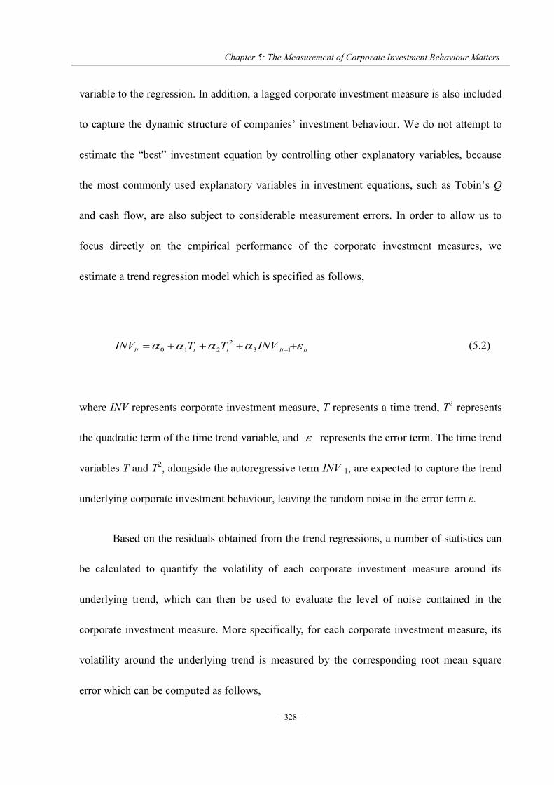
Chapter 5: The Measurement of Corporate Investment Behaviour Matters
– 328 –
variable to the regression. In addition, a lagged corporate investment measure is also included
to capture the dynamic structure of companies’ investment behaviour. We do not attempt to
estimate the “best” investment equation by controlling other explanatory variables, because
the most commonly used explanatory variables in investment equations, such as Tobin’s Q
and cash flow, are also subject to considerable measurement errors. In order to allow us to
focus directly on the empirical performance of the corporate investment measures, we
estimate a trend regression model which is specified as follows,
ititttit INVTTINV 132
210 (5.2)
where INV represents corporate investment measure, T represents a time trend, T2 represents
the quadratic term of the time trend variable, and represents the error term. The time trend
variables T and T2, alongside the autoregressive term INV–1, are expected to capture the trend
underlying corporate investment behaviour, leaving the random noise in the error term ε.
Based on the residuals obtained from the trend regressions, a number of statistics can
be calculated to quantify the volatility of each corporate investment measure around its
underlying trend, which can then be used to evaluate the level of noise contained in the
corporate investment measure. More specifically, for each corporate investment measure, its
volatility around the underlying trend is measured by the corresponding root mean square
error which can be computed as follows,

Chapter 5: The Measurement of Corporate Investment Behaviour Matters
– 329 –
NVNIINV itit
2)ˆ(RMSE (5.3)
where RMSE represents the root mean square error, INV and VNI ˆ represent the observed
and fitted value of corporate investment measures respectively and N represents the total
sample size. According to its definition, the RMSE aggregates the individual residuals into a
single measure of volatility around the underlying trend for each of the corporate investment
measures. For unbiased estimators, the RMSE can be considered as the standard error of the
residuals from the trend regression. Like the standard error, the RMSE is on the same scale as
the observed variable, and thus it cannot be used to compare the volatilities across various
corporate investment measures with different scales. Hyndman and Koehler (2006) point out
that the RMSE of a regression must be understood in the context of the mean of the observed
variable. Accordingly, we further calculate the coefficient of variation of the root mean square
error for each of the corporate investment measures by scaling the RMSE with the
corresponding absolute mean of the corporate investment measures. The coefficient of
variation of the root mean square error is a similar concept to the coefficient of variation, and
is defined as follows,
VNIRMSECV(RMSE)
(5.4)

Chapter 5: The Measurement of Corporate Investment Behaviour Matters
– 330 –
where CV(RMSE) represents the coefficient of variation of the root mean square error, and
VNI represents the mean of the observed corporate investment measure. Thus, the
CV(RMSE) is a dimensionless statistic which can be used to compare the volatilities of
various corporate investment measures around their respective trends. It is worth noting that,
like the coefficient of variation, the usefulness of the coefficient of variation of the root mean
squared error is limited when the mean value of the observed variable is close to zero.
5.6.2 Empirical results
Table 5.5 presents the system-GMM estimation results of the trend regression specified as
Equation 5.2 for each of the corporate investment measures. As is evident, the time trend
variables are highly significant in their linear as well as quadratic forms in almost all
regressions. Estimated coefficients for the linear time trend term are uniformly negative,
whereas those for the quadratic term are consistently positive, indicating that corporate
investment behaviour trends around a U-shaped curve over the period 1999–2008. In addition,
the autoregressive term turns out to be positive in all of the regressions, and statistically
significant in most cases, suggesting the existence of a dynamic structure in corporate
investment behaviour. Moreover, the results of the diagnostic tests for the trend regressions
also suggest that the model specification is reasonably well and the instruments used are
generally valid. Therefore, the residuals from the estimated trend regressions can be
satisfactorily used to assess the level of noise contained in the corporate investment measures.
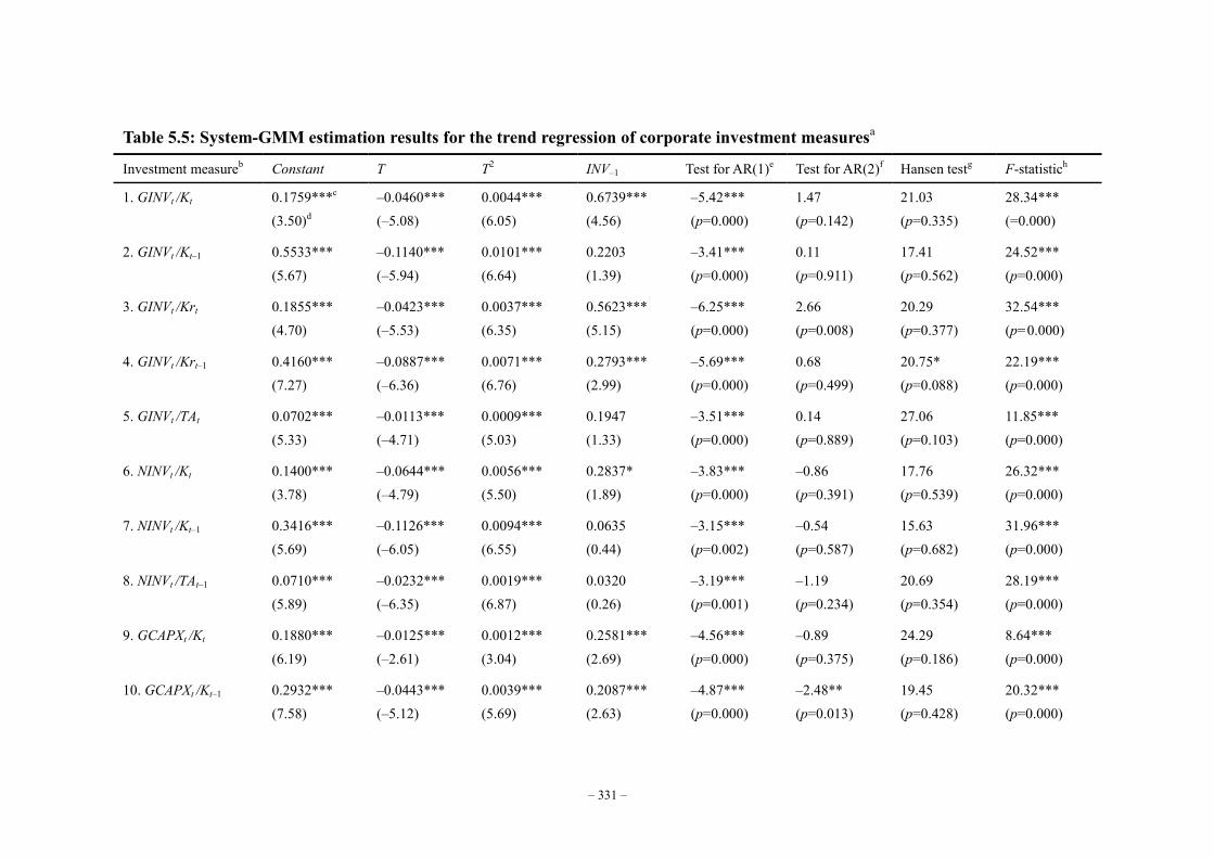
– 331 –
Table 5.5: System-GMM estimation results for the trend regression of corporate investment measuresa
Investment measureb Constant T T2 INV–1 Test for AR(1)e Test for AR(2)f Hansen testg F-statistich
1. GINVt /Kt 0.1759***c (3.50)d
–0.0460*** (–5.08)
0.0044*** (6.05)
0.6739*** (4.56)
–5.42*** (p=0.000)
1.47 (p=0.142)
21.03 (p=0.335)
28.34*** (=0.000)
2. GINVt /Kt–1 0.5533*** (5.67)
–0.1140*** (–5.94)
0.0101*** (6.64)
0.2203 (1.39)
–3.41*** (p=0.000)
0.11 (p=0.911)
17.41 (p=0.562)
24.52*** (p=0.000)
3. GINVt /Krt 0.1855*** (4.70)
–0.0423*** (–5.53)
0.0037*** (6.35)
0.5623*** (5.15)
–6.25*** (p=0.000)
2.66 (p=0.008)
20.29 (p=0.377)
32.54*** (p=0.000)
4. GINVt /Krt–1 0.4160*** (7.27)
–0.0887*** (–6.36)
0.0071*** (6.76)
0.2793*** (2.99)
–5.69*** (p=0.000)
0.68 (p=0.499)
20.75* (p=0.088)
22.19*** (p=0.000)
5. GINVt /TAt 0.0702*** (5.33)
–0.0113*** (–4.71)
0.0009*** (5.03)
0.1947 (1.33)
–3.51*** (p=0.000)
0.14 (p=0.889)
27.06 (p=0.103)
11.85*** (p=0.000)
6. NINVt /Kt 0.1400*** (3.78)
–0.0644*** (–4.79)
0.0056*** (5.50)
0.2837* (1.89)
–3.83*** (p=0.000)
–0.86 (p=0.391)
17.76 (p=0.539)
26.32*** (p=0.000)
7. NINVt /Kt–1 0.3416*** (5.69)
–0.1126*** (–6.05)
0.0094*** (6.55)
0.0635 (0.44)
–3.15*** (p=0.002)
–0.54 (p=0.587)
15.63 (p=0.682)
31.96*** (p=0.000)
8. NINVt /TAt–1 0.0710*** (5.89)
–0.0232*** (–6.35)
0.0019*** (6.87)
0.0320 (0.26)
–3.19*** (p=0.001)
–1.19 (p=0.234)
20.69 (p=0.354)
28.19*** (p=0.000)
9. GCAPXt /Kt 0.1880*** (6.19)
–0.0125*** (–2.61)
0.0012*** (3.04)
0.2581*** (2.69)
–4.56*** (p=0.000)
–0.89 (p=0.375)
24.29 (p=0.186)
8.64*** (p=0.000)
10. GCAPXt /Kt–1 0.2932*** (7.58)
–0.0443*** (–5.12)
0.0039*** (5.69)
0.2087*** (2.63)
–4.87*** (p=0.000)
–2.48** (p=0.013)
19.45 (p=0.428)
20.32*** (p=0.000)
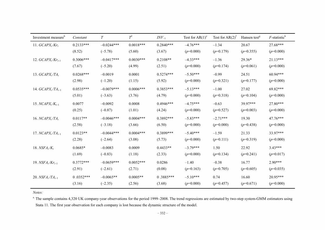
– 332 –
Investment measureb Constant T T2 INV–1 Test for AR(1)e Test for AR(2)f Hansen testg F-statistich
11. GCAPXt /Krt 0.2133*** (8.52)
–0.0244*** (–5.78)
0.0018*** (5.60)
0.2840*** (3.67)
–4.76*** (p=0.000)
–1.34 (p=0.179)
20.67 (p=0.355)
27.68*** (p=0.000)
12. GCAPXt /Krt–1 0.3006*** (7.67)
–0.0417*** (–5.20)
0.0030*** (4.99)
0.2108** (2.51)
–4.33*** (p=0.000)
–1.36 (p=0.174)
29.36* (p=0.061)
21.13*** (p=0.000)
13. GCAPXt /TAt 0.0268*** (2.98)
–0.0019 (–1.20)
0.0001 (1.15)
0.5274*** (5.92)
–5.50*** (p=0.000)
–0.99 (p=0.321)
24.51 (p=0.177)
60.94*** (p=0.000)
14. GCAPXt /TAt–1 0.0535*** (5.01)
–0.0079*** (–3.63)
0.0006*** (3.76)
0.3853*** (4.79)
–5.13*** (p=0.000)
–1.00 (p=0.318)
27.02 (p=0.104)
69.82*** (p=0.000)
15. NCAPXt /Kt–1 0.0077 (0.25)
–0.0092 (–0.87)
0.0008 (1.01)
0.4946*** (4.24)
–4.75*** (p=0.000)
–0.63 (p=0.527)
39.97*** (p=0.003)
27.80*** (p=0.000)
16. NCAPXt /TAt 0.0117** (2.58)
–0.0046*** (–3.18)
0.0004*** (3.66)
0.3892*** (6.50)
–5.83*** (p=0.000)
–2.71*** (p=0.000)
19.30 (p=0.438)
47.76*** (p=0.000)
17. NCAPXt /TAt–1 0.0123** (2.28)
–0.0044*** (–2.64)
0.0004*** (3.08)
0.3899*** (5.73)
–5.40*** (p=0.000)
–1.59 (p=0.111)
21.33 (p=0.319)
33.97*** (p=0.000)
18. NSFAt /Kt 0.0685* (1.69)
–0.0083 (–0.83)
0.0009 (1.18)
0.4433** (2.33)
–3.79*** (p=0.000)
1.50 (p=0.134)
22.92 (p=0.241)
3.43*** (p=0.017)
19. NSFAt /Krt–1 0.3772*** (2.91)
–0.0659*** (–2.61)
0.0052*** (2.71)
0.0286 (0.08)
–1.40 (p=0.163)
–0.38 (p=0.705)
16.77 (p=0.605)
2.90*** (p=0.035)
20. NSFAt /TAt–1 0 .0352*** (3.16)
–0.0065** (–2.35)
0.0005** (2.56)
0 .3885*** (3.68)
–5.10*** (p=0.000)
0.74 (p=0.457)
16.60 (p=0.671)
20.95*** (p=0.000)
Notes: a. The sample contains 4,320 UK company-year observations for the period 1999–2008. The trend regressions are estimated by two-step system-GMM estimators using
Stata 11. The first year observation for each company is lost because the dynamic structure of the model.

– 333 –
b. Different corporate investment measures are used as the dependent variable in their respective time trend regressions. The time trend regression is specified as
ititttit INVTTINV 132
210 . The instruments used for the regression include Constant, T, T2, INVt-3… t-5, ∆T, ∆T2, and ∆INVt-2.
c. * significant at the 10% level; ** significant at the 5% level; and *** significant at the 1% level. d. t-statistics are reported in parentheses. e. The Arellona-Bond test tests for serial correlation in the first-differenced errors in order to purge the unobserved and perfectly autocorrelated individual effects.
Autocorrelation at order 1 is expected in first differences, because 1 ititit should correlate with 211 ititit , since they share the 1it term. f. To check for AR(1) in levels, look for AR(2) in differences, in the idea that this will detect the relationship between the 1it in it and the 2it in 2 it .
Autocorrelation indicates that lags of the dependent variable (and any other variables used as instruments that are not strictly exogenous), are in fact endogenous, thus bad instruments. Therefore, rejecting the null hypothesis of no serial correlation in the first-differenced errors at an order greater than one implies model misspecification.
g. The Hansen overidentifying restrictions test tests for whether the instruments, as a group, appear exogenous. Under two-step robust GMM estimation, the Sargan statistic is not robust to heteroscedasticity or autocorrelation, but the Hensen J-statistic, which is the minimised value of the two-step GMM criterion function, is robust. The joint null hypothesis is that the instruments are valid instruments, i.e. uncorrelated with the error term, and that the excluded instruments are correctly excluded from the estimated equation. A statistically significant test statistic always indicates that the instruments may not be valid. However, the J-test has its own problem: it can be greatly weakened by instrument proliferation.
h. F-statistic for the regression which tests the null hypothesis that all of the coefficients except the intercept coefficient are jointly zero.
Chapter 5: The Measurement of Corporate Investment Behaviour Matters
– 334 –
Based on the residuals obtained by estimating the trend regression as specified in
Equation 5.2, the RMSE, absolute mean and CV(RMSE) for each of the corporate investment
measures are calculated and reported in Table 5.6. In addition, according to their respective
CV(RMSE)s, the corporate investment measures are ranked from lowest volatility to highest
volatility. Several features of these results are of particular interest.
First, corporate investment measures in the highest ranked (lowest volatility) group are
without exception gross investment measures, and those in the lowest ranked (highest
volatility) group are all net investment measures. This finding suggests that the gross
corporate investment measures are systematically less volatile around their respective trends
than the net corporate investment measures. Our results indicate that if depreciated capital
goods are taken into account, corporate investment behaviour becomes more volatile and thus
less predictable. The excess volatility of the net corporate investment measures over the gross
investment measures is directly attributable to the depreciation component which is
potentially subject to managers’ opportunistic manipulation. Our empirical evidence,
therefore, lends strong support to the prediction that net corporate investment measures,
which are jointly determined by gross investment and depreciation expense, are noisier than
gross corporate investment measures, and thus Hypothesis 3 should be firmly rejected.
However, the high CV(RMSE) values for the net corporate investment measures may also be
attributable to their low mean values, and therefore the results should be interpreted with
caution.
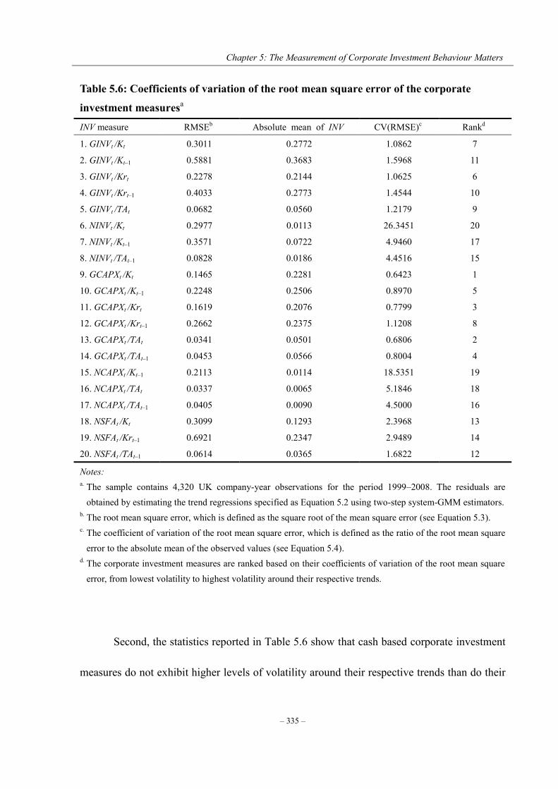
Chapter 5: The Measurement of Corporate Investment Behaviour Matters
– 335 –
Table 5.6: Coefficients of variation of the root mean square error of the corporate
investment measuresa
INV measure RMSEb Absolute mean of INV CV(RMSE)c Rankd
1. GINVt /Kt 0.3011 0.2772 1.0862 7
2. GINVt /Kt–1 0.5881 0.3683 1.5968 11
3. GINVt /Krt 0.2278 0.2144 1.0625 6
4. GINVt /Krt–1 0.4033 0.2773 1.4544 10
5. GINVt /TAt 0.0682 0.0560 1.2179 9
6. NINVt /Kt 0.2977 0.0113 26.3451 20
7. NINVt /Kt–1 0.3571 0.0722 4.9460 17
8. NINVt /TAt–1 0.0828 0.0186 4.4516 15
9. GCAPXt /Kt 0.1465 0.2281 0.6423 1
10. GCAPXt /Kt–1 0.2248 0.2506 0.8970 5
11. GCAPXt /Krt 0.1619 0.2076 0.7799 3
12. GCAPXt /Krt–1 0.2662 0.2375 1.1208 8
13. GCAPXt /TAt 0.0341 0.0501 0.6806 2
14. GCAPXt /TAt–1 0.0453 0.0566 0.8004 4
15. NCAPXt /Kt–1 0.2113 0.0114 18.5351 19
16. NCAPXt /TAt 0.0337 0.0065 5.1846 18
17. NCAPXt /TAt–1 0.0405 0.0090 4.5000 16
18. NSFAt /Kt 0.3099 0.1293 2.3968 13
19. NSFAt /Krt–1 0.6921 0.2347 2.9489 14
20. NSFAt /TAt–1 0.0614 0.0365 1.6822 12
Notes: a. The sample contains 4,320 UK company-year observations for the period 1999–2008. The residuals are
obtained by estimating the trend regressions specified as Equation 5.2 using two-step system-GMM estimators. b. The root mean square error, which is defined as the square root of the mean square error (see Equation 5.3). c. The coefficient of variation of the root mean square error, which is defined as the ratio of the root mean square
error to the absolute mean of the observed values (see Equation 5.4). d. The corporate investment measures are ranked based on their coefficients of variation of the root mean square
error, from lowest volatility to highest volatility around their respective trends.
Second, the statistics reported in Table 5.6 show that cash based corporate investment
measures do not exhibit higher levels of volatility around their respective trends than do their

Chapter 5: The Measurement of Corporate Investment Behaviour Matters
– 336 –
accrual based counterparts. Although accrual based accounting figures are typically
considered as smoothed measures of cash flow based accounting figures since they are
supposed to mitigate the timing and mismatching problems of cash flows, we do not find
empirical evidence that accrual based corporate investment measures are systematically less
noisy than cash based measures. Surprisingly, for gross corporate investment measures, cash
based measures appear to be systematically less volatile around their respective trends than
accrual based measures, as indicated by the CV(RMSE)s. This is largely due to the fact that
accrual based measures of corporate investment, according to accounting standards, take asset
revaluations and writedowns as well as disinvestments into account, which introduce
additional fluctuations into these measures. On the other hand, cash based measures focus on
the amount of funds spent by a company on its fixed assets and are not affected by the amount
of disinvestment, and therefore behave relatively stable over time. According to our results,
we do not find any empirical evidence that cash based corporate investment measures are
nosier than their accrual based counterparts, and thus Hypothesis 2 cannot be rejected.
Third, the results presented in Table 5.6 also show that the cash based measures of net
spending on fixed assets (i.e. NSFAt /Kt, NSFAt /Krt–1 and NSFAt /TAt–1), which take into
account the revenue from the sales of fixed assets, are more volatile than gross corporate
investment measures due to the additional volatilities brought in by disinvesting activities.
However, they are less volatile than the net corporate investment measures, indicating that
depreciation which may opportunistically manipulated by management is the most volatile

Chapter 5: The Measurement of Corporate Investment Behaviour Matters
– 337 –
and unpredictable component in measuring corporate investment behaviour, although it has
been conventionally considered as a process of smoothly allocating the cost of a tangible
fixed asset over its useful life.
5.6.3 Robustness tests and results
To assess the robustness of our trend analysis results, we also carry out further estimation and
testing procedures to gauge the sensitivity of our results with respect to the measurement of
volatility, estimation techniques and model specifications.
First, instead of using the RMSE, we calculate the mean absolute error (MAE) to
measure the volatilities of the corporate investment measures around their respective trends.
Hyndman and Koehler (2006) highlight an attractive additional property of the MAE that it is
less sensitive to outliers compared to the RMSE. As shown in Appendix 5.H, the results based
on the MAE are consistent with those based on the RMSE reported in Table 5.6. Although the
orders of corporate investment measures ranked by different statistics are slightly different,
our conclusions drawn from the trend analysis remain hold.
Second, we re-estimate the trend regression model specified as Equation 5.2 using
difference-GMM estimators. The difference-GMM estimation results reported in Appendix
5.I are similar to those obtained from system-GMM estimation in terms of the signs and
significant levels of the estimated coefficients. As can be seen from Appendix 5.J, the ranking
of the corporate investment measures based on the difference-GMM estimation residuals are
Chapter 5: The Measurement of Corporate Investment Behaviour Matters
– 338 –
also generally consistent with our earlier evidence presented in Table 5.6.
Third, we examine how robust the results of trend analysis are with respect to the
specification of the lag structure of the corporate investment measure in the regressions. In
addition to the lagged dependent variable (INV–1), we also include a corporate investment
measure which is lagged twice (INV–2) as an additional explanatory variable. The coefficients
estimated for the additional lagged dependent variable are statistically insignificant in most of
the regressions. Meanwhile, the inclusion of the additional lagged dependent variable also
suppresses the explanatory power of other explanatory variables. However, the ranking of the
corporate investment measures produced under this alternative specification of lag structure is
largely consistent with our main results reported in Table 5.6. It is also found that corporate
investment measures lagged beyond two periods have little explanatory power in all of the
regressions.
Besides, we also estimate a trend regression in which the time trend is included only
as a linear term rather than as linear and quadratic terms. We find that the linear time trend
term becomes statistically insignificant when the quadratic term is ignored, which suggests
that the underlying trend of corporate investment behaviour over the period under
investigation is indeed nonlinear.
5.6.4 Conclusion
In summary, the trend analysis of the corporate investment measures shows that the
investment behaviour of UK-listed companies follows a U-shaped trend over the period
Chapter 5: The Measurement of Corporate Investment Behaviour Matters
– 339 –
1999–2008. It is found that the gross investment measures are systematically less volatile
around their respective trends, and thus are less noisy than the net investment measures. The
excess volatility of net investment measures is largely due to the noise contained in
depreciation expense which is subject to opportunistic manipulation by management.
However, our empirical results do not show any evidence that cash based measures contain
higher levels of noise than do their accrual based counterparts. In fact, it is suggested that cash
based gross investment measures exhibit the lowest volatilities around their respective trends
among the alternatives. The trend analysis results presented in this section are robust with
respect to the measurement of volatility, model specification and estimation techniques.
5.7 Information content analysis
We turn now to the information content of the corporate investment measures. Information
content analysis has been used extensively in accounting studies to address different research
questions (see Biddle et al., 1995). However, few previous studies have applied information
content comparisons in the field of corporate investment. Two exceptions are Park and Pincus
(2003) and Kerstein and Kim (1995), who explicitly examine the incremental information
about a company’s future earnings provided by capital expenditures which is not captured by
current earnings. To the best of our knowledge, no attempt has been made to provide a
comparison of the information content of the alternative corporate investment measures. To
fill the gap, this section examines whether the alternative corporation investment measures

Chapter 5: The Measurement of Corporate Investment Behaviour Matters
– 340 –
yield value relevant information which is incremental to that of current earnings; and if they
do, which measures have the greatest value relevant incremental information content.
5.7.1 Incremental and relative information content
There are two types of information content analysis, namely, relative information content
analysis and incremental information content analysis. Adam and Goyal (2008) indicate that
incremental comparison is useful in determining whether one variable provides information
beyond that provided by another, while relative comparison is useful in determining which
variable has the greatest information content among the alternatives.51
The logical relations between the relative and incremental information content
comparisons of two variables (say X and Y, for example) can be illustrated by the Venn
diagrams presented in Figure 5.1, which adopted from Biddle et al. (1995). The areas covered
by the circles, as defined by Biddle et al. (1995), represent the proportion of variation in a
dependent variable explained by predictor variables X and Y, i.e. the relative information
content of the two predictor variables with respect to the dependent variable. The left hand
column of Figure 5.1 portrays three possible relationships between the relative information
contents of X and Y, while the right hand column portrays the corresponding possible
relationships between X and Y in terms of their incremental information content with respect
to each other.
51 Biddle et al. (1995) also point out that relative information content analysis applies when making mutually exclusive choices among alternatives, or when rankings by information content are desired.

Chapter 5: The Measurement of Corporate Investment Behaviour Matters
– 341 –
Figure 5.1: Logical relation between incremental and relative information content of two
variablesa Panel A: X and Y have equal relative information content
b
=
X and Y have equal relative information
content Neither X or Y is
incremental Both X and Y are
incremental
Panel B: X has larger relative information content than Y
>
X has larger relative information content than Y
Only X is incremental
Both X and Y are incremental
Panel C: X has smaller relative information content than Y
<
X has smaller relative information content than Y
Only Y is incremental
Both X and Y are incremental
Notes: a. Adopted from Biddle et al. (1995), Figure 1 on page 4. b. Areas covered by circles represent variation in a dependent variable explained by predictor variables X and Y.
Variables X and Y depicted in Panel A of Figure 5.1 have equal relative information
content as indicated by the equal size of the two circles (i.e. X = Y). If the information content
Y X, Y X Y
X X X
Y Y Y
Y
X
Y Y
X
X X

Chapter 5: The Measurement of Corporate Investment Behaviour Matters
– 342 –
provided by the two variables is exactly the same, then the two circles coincide and neither X
or Y is incremental with respect to each other (i.e. YXYX ). But if they provide
different sets of information related to the dependent variable, both of them are incremental.
This is because the information content of X and Y together is greater than that of one variable
alone (i.e. XYX and YYX ). The intersection of the two circles (i.e. YX )
represents the overlapping information contained in both X and Y, which can be quantified by
the correlation between X and Y. The area in Y but not in X represents the incremental
information content provided by Y beyond that provided by X, and vice versa.
In Panel B of Figure 5.1, the size of the circle for X is larger than that for Y, indicating
that variable X has greater relative information content than Y (i.e. X >Y). There are also two
possible incremental information content outcomes. If Y is a subset of X (i.e. XY ), then the
information content provided by Y is already included in X and therefore only X is incremental.
However, as long as Y is not entirely included in X, then both variables X and Y are
incremental. In this case, although Y has smaller relative information content, it also provides
additional information content beyond that provided by X, contributing to the information
content of the union of the two variables. Similarly, Panel C of Figure 5.1 portrays the
relationship between relative and incremental information content under the condition that X
has smaller relative information content than Y.
To sum up, the relationships between relative and incremental information are not a
one-to-one correspondence. Each relative information content condition can be matched to at
Chapter 5: The Measurement of Corporate Investment Behaviour Matters
– 343 –
least two incremental outcome conditions as shown in each of the panels of Figure 5.1. The
relative information content of a variable is determined by its explanatory power for the
variability of the dependent variable, which can be visualised by the size of a circle in Figure
5.1, while the variable’s incremental information content with respect to another variable is
determined by the additional explanatory power it provides, as reflected by the position of the
circle relative to another circle.
5.7.2 Empirical procedures
In the context of corporate finance, it is generally believed that changes in corporate
investment yield information about the changes in a company’s future prospects that is not
captured by the company’s unexpected current earnings (see Park and Pincus, 2003; and
Kerstein and Kim, 1995). It is argued that, if the capital market is strong form efficient,
corporate investment decisions would not be value relevant, because the information based on
which investment decisions are made should be fully available to the capital market and
appropriately reflected in the security prices. However, in the real world, where information
asymmetry exists, managers know more than outsiders about a company’s future prospects,
and they may use their private information to make corporate investment decisions. Under
such circumstances, unexpected changes in corporate investment would signal managers’
private information, such as the availability of valuable investment opportunities to the
company and the growth opportunities of the industry, to the capital market. Therefore,
Kerstein and Kim (1995) predict that, because managers may respond to the private
Chapter 5: The Measurement of Corporate Investment Behaviour Matters
– 344 –
information about their company’s future prospects through their investment decisions,
unexpected corporate investments are expected to be reflected in the company’s stock returns
in a forward-looking capital market, providing value relevant information beyond that
provided by the company’s current earnings.
To formally assess the information content of the alternative corporate investment
measures, we adopt the regression-based methodology developed by Biddle et al. (1995).
Specifically, we first examine whether corporate investment measures provide value relevant
information content beyond that of current earnings by regressing market adjusted return on
unexpected current earnings and unexpected corporate investment. More specifically, we
estimate the regression model specified as follows,
itititit eUINVUEPSMAR 210 (5.5)
where MARit denotes market adjusted return for company i over year t, which is calculated as
the sum of capital gains and dividend incomes per share deflated by the share price at the
beginning of the period, and then adjusted to the stock market return over the same period;
UEPSit denotes unexpected earnings per share of company i’s common stock in year t scaled
by the beginning of the period share price; and UINVit denotes unexpected change in the
measure of investment ratio for company i in year t. Following the previous studies of Park
Chapter 5: The Measurement of Corporate Investment Behaviour Matters
– 345 –
and Pincus (2003) and Kerstein and Kim (1995), we assume that both earnings per share and
corporate investment follow a random walk process, so that the entire change in these two
variables from one period to the next is considered as unexpected change.
The model specified in Equation 5.5 first tests whether changes in corporate
investment provide information about company’s future earnings growth opportunities in the
presence of current earnings surprises, by examining the sign and significance level of the
coefficient estimated for UINV (Kerstein and Kim, 1995). If the measures of corporate
investment do indeed provide incremental value relevant information after controlling for the
unexpected changes in earnings per share, the coefficient estimated for the changes
incorporate investment variable is expected to be positive and statistically significant.
If unexpected corporate investment is incremental with respect to unexpected current
earnings, our primary focus will be shifted to the comparison of the relative information
content of the alternative corporate investment measures. The corporate investment measures
that have greater relative information content are expected to be statistically more significant
in their respective regressions. The significance level of the unexpected corporate investment
variable in the regression model can be tested using the Wald test. Under the Wald test, the
null hypothesis that unexpected corporate investment is not informative should be rejected
more resoundingly if the corporate investment measure being tested has greater information
content on a relative scale. Therefore, the information content of the corporate investment
measures can be ranked based on their respective Wald test results.
Chapter 5: The Measurement of Corporate Investment Behaviour Matters
– 346 –
5.7.3 Empirical results
The system-GMM estimation results for the regression of market adjusted returns on
unexpected earnings and unexpected corporate investment, as specified in Equation 5.5, are
reported in Table 5.7. As expected, the coefficients estimated for UEPS are highly significant
in all regressions, indicating that unexpected current earnings have significant explanatory
power for the market adjusted returns. More importantly, it is found that changes in corporate
investment measures have the predicted positive sign everywhere and are statistically
significant in 19 out of 20 regressions. The significantly positive coefficients found for UINV
clearly show that unexpected corporate investment does indeed provide value relevant
information which is incremental to that provided by current earnings. We, therefore,
conclude that unexpected current earnings and unexpected corporate investment are
incremental with respect to each other, and market adjusted returns are sensitive to both of
them. The results presented in Table 5.7 are highly consistent with the theoretical argument as
well as the empirical evidence provided by previous studies (see, for example, Park and
Pincus, 2003; and Kerstein and Kim, 1995). Besides, results of the Arellona-Bond test for
serial correlations and the Hansen test for overidentifying restrictions reported in Table 5.7
suggest that the model used to assess the information content of corporate investment
measures is well specified, and the instruments used to implement the system-GMM
estimation are generally valid.
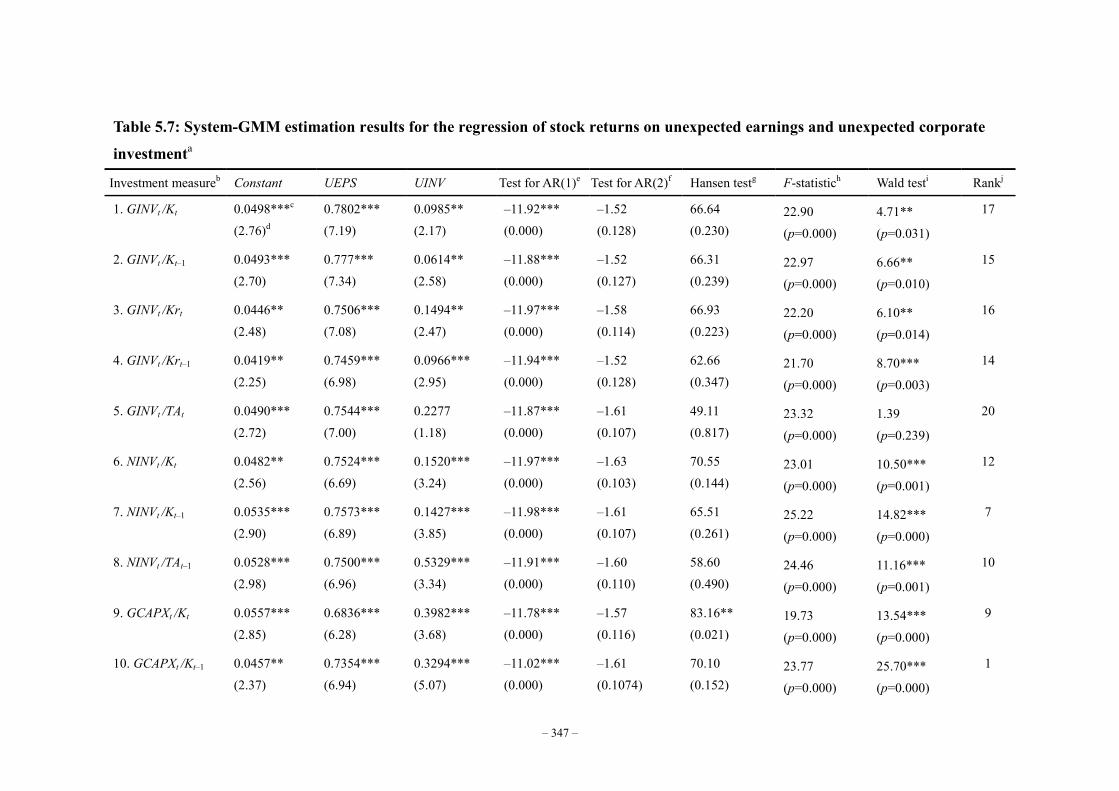
– 347 –
Table 5.7: System-GMM estimation results for the regression of stock returns on unexpected earnings and unexpected corporate
investmenta
Investment measureb Constant UEPS UINV Test for AR(1)e Test for AR(2)f Hansen testg F-statistich Wald testi Rankj
1. GINVt /Kt 0.0498***c (2.76)d
0.7802*** (7.19)
0.0985** (2.17)
–11.92*** (0.000)
–1.52 (0.128)
66.64 (0.230)
22.90 (p=0.000)
4.71** (p=0.031)
17
2. GINVt /Kt–1 0.0493*** (2.70)
0.777*** (7.34)
0.0614** (2.58)
–11.88*** (0.000)
–1.52 (0.127)
66.31 (0.239)
22.97 (p=0.000)
6.66** (p=0.010)
15
3. GINVt /Krt 0.0446** (2.48)
0.7506*** (7.08)
0.1494** (2.47)
–11.97*** (0.000)
–1.58 (0.114)
66.93 (0.223)
22.20 (p=0.000)
6.10** (p=0.014)
16
4. GINVt /Krt–1 0.0419** (2.25)
0.7459*** (6.98)
0.0966*** (2.95)
–11.94*** (0.000)
–1.52 (0.128)
62.66 (0.347)
21.70 (p=0.000)
8.70*** (p=0.003)
14
5. GINVt /TAt 0.0490*** (2.72)
0.7544*** (7.00)
0.2277 (1.18)
–11.87*** (0.000)
–1.61 (0.107)
49.11 (0.817)
23.32 (p=0.000)
1.39 (p=0.239)
20
6. NINVt /Kt 0.0482** (2.56)
0.7524*** (6.69)
0.1520*** (3.24)
–11.97*** (0.000)
–1.63 (0.103)
70.55 (0.144)
23.01 (p=0.000)
10.50*** (p=0.001)
12
7. NINVt /Kt–1 0.0535*** (2.90)
0.7573*** (6.89)
0.1427*** (3.85)
–11.98*** (0.000)
–1.61 (0.107)
65.51 (0.261)
25.22 (p=0.000)
14.82*** (p=0.000)
7
8. NINVt /TAt–1 0.0528*** (2.98)
0.7500*** (6.96)
0.5329*** (3.34)
–11.91*** (0.000)
–1.60 (0.110)
58.60 (0.490)
24.46 (p=0.000)
11.16*** (p=0.001)
10
9. GCAPXt /Kt 0.0557*** (2.85)
0.6836*** (6.28)
0.3982*** (3.68)
–11.78*** (0.000)
–1.57 (0.116)
83.16** (0.021)
19.73 (p=0.000)
13.54*** (p=0.000)
9
10. GCAPXt /Kt–1 0.0457** (2.37)
0.7354*** (6.94)
0.3294*** (5.07)
–11.02*** (0.000)
–1.61 (0.1074)
70.10 (0.152)
23.77 (p=0.000)
25.70*** (p=0.000)
1
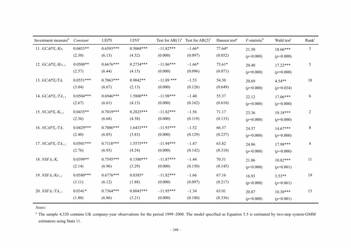
– 348 –
Investment measureb Constant UEPS UINV Test for AR(1)e Test for AR(2)f Hansen testg F-statistich Wald testi Rankj
11. GCAPXt /Krt 0.0453** (2.30)
0.6593*** (6.13)
0.5068*** (4.32)
–11.82*** (0.000)
–1.66* (0.097)
77.64* (0.052)
21.50 (p=0.000)
18.66*** (p=0.000)
3
12. GCAPXt /Krt–1 0.0508** (2.57)
0.6676*** (6.44)
0.2734*** (4.15)
–11.86*** (0.000)
–1.66* (0.096)
75.61* (0.071)
20.40 (p=0.000)
17.22*** (p=0.000)
5
13. GCAPXt/TAt 0.0551*** (3.04)
0.7063*** (6.67)
0.9042** (2.13)
–11.89 *** (0.000)
–1.53 (0.126)
54.30 (0.649)
20.69 (p=0.000)
4.54** (p=0.034)
18
14. GCAPXt /TAt–1 0.0504*** (2.67)
0.6946*** (6.61)
1.5800*** (4.13)
–11.98*** (0.000)
–1.40 (0.162)
55.37 (0.610)
22.12 (p=0.000)
17.06*** (p=0.000)
6
15. NCAPXt /Kt–1 0.0435** (2.36)
0.7019*** (6.68)
0.2825*** (4.38)
–11.82*** (0.000)
–1.56 (0.119)
71.17 (0.133)
23.36 (p=0.000)
19.18*** (p=0.000)
2
16. NCAPXt /TAt 0.0429*** (2.40)
0.7006*** (6.85)
1.6433*** (3.83)
–11.93*** (0.000)
–1.52 (0.129)
66.37 (0.237)
24.57 (p=0.000)
14.67*** (p=0.000)
8
17. NCAPXt /TAt–1 0.0501*** (2.76)
0.7118*** (6.93)
1.5575*** (4.24)
–11.94*** (0.000)
–1.47 (0.142)
63.82 (0.310)
24.86 (p=0.000)
17.98*** (p=0.000)
4
18. NSFAt /Kt 0.0399** (2.14)
0.7595*** (6.96)
0.1580*** (3.29)
–11.87*** (0.000)
–1.44 (0.150)
70.51 (0.145)
21.06 (p=0.000)
10.82*** (p=0.001)
11
19. NSFAt /Krt–1 0.0580*** (3.11)
0.6776*** (6.12)
0.0385* (1.88)
–11.82*** (0.000)
–1.66 (0.097)
67.16 (0.217)
16.93 (p=0.000)
3.53** (p=0.061)
19
20. NSFAt /TAt–1 0.0341* (1.80)
0.7364*** (6.86)
0.8043*** (3.21)
–11.95*** (0.000)
–1.34 (0.180)
63.01 (0.336)
20.87 (p=0.000)
10.30*** (p=0.001)
13
Notes: a. The sample 4,320 contains UK company-year observations for the period 1999–2008. The model specified as Equation 5.5 is estimated by two-step system-GMM
estimators using Stata 11.

– 349 –
b. Unexpected change in corporate investment measures are used as an explanatory variable in their respective regressions. The regression is specified as
itititit eUINVUEPSMAR 210 We also control for time effects by adding a set of year dummy variables. The instruments used for the regression include Constant, Year dummies, UEPSt-1…, t-3, UINVt-1…, t-3, ∆Year dummies, ∆UEPSt and ∆UINVt.
c. * significant at the 10% level; ** significant at the 5% level; and *** significant at the 1% level. d. t-statistics are reported in parentheses. e. The Arellona-Bond test tests for serial correlation in the first-differenced errors in order to purge the unobserved and perfectly autocorrelated individual effects.
Autocorrelation at order 1 is expected in first differences, because 1 ititit should correlate with 211 ititit , since they share the 1it term. f. To check for AR(1) in levels, look for AR(2) in differences, in the idea that this will detect the relationship between the 1it in it and the 2it in 2 it .
Autocorrelation indicates that lags of the dependent variable (and any other variables used as instruments that are not strictly exogenous), are in fact endogenous, thus bad instruments. Therefore, rejecting the null hypothesis of no serial correlation in the first-differenced errors at an order greater than one implies model misspecification.
g. The Hansen overidentifying restrictions test tests for whether the instruments, as a group, appear exogenous. Under two-step robust GMM estimation, the Sargan statistic is not robust to heteroscedasticity or autocorrelation, but the Hensen J-statistic, which is the minimised value of the two-step GMM criterion function, is robust. The joint null hypothesis is that the instruments are valid instruments, i.e. uncorrelated with the error term, and that the excluded instruments are correctly excluded from the estimated equation. A statistically significant test statistic always indicates that the instruments may not be valid. However, the J-test has its own problem: it can be greatly weakened by instrument proliferation.
h. F-statistic for the regression which tests the null hypothesis that all of the coefficients except the intercept coefficient are jointly zero. i. We perform Wald test to test the null hypothesis that the coefficient on UINV is equal to zero. The test reports results using the F-statistic. The associated p-value is
reported in parenthesis. j. The corporate investment measures are ranked based on their respective Wald test results from the highest informative to lowest informative.
Chapter 5: The Measurement of Corporate Investment Behaviour Matters
– 350 –
We now focus on the relative information content of the alternative corporate
investment measures. The Wald test is carried out to test the significance of the unexpected
corporate investment variable in each regression. The Wald test results are reported in Table
5.7. In addition, the alternative corporate investment measures are ranked from the most
informative to the least informative based on their respective Wald test results. It is found that
cash based corporate investment measures are systematically more informative compared to
their accrual based counterparts. This finding lends strong support to the prediction that
investors are more concerned with cash flow based measures, which are less subject to
distortions from differing accounting practices. The accrual based corporate investment
measures, which are more likely to be distorted by the choices of discretionary accounting
policies and by managers’ opportunistic manipulations, are thus less relevant to company
value. Therefore, our empirical evidence rejects Hypothesis 4 that cash based and accrual
based corporate investment measures are equally informative, in favour of the alternative
hypothesis that cash based measures are relatively more informative.
Besides, the results presented in Table 5.7 do not show any systematic difference
between the gross and net corporate investment measures in terms of their value relevant
information content. However, for the accrual based measures, net corporate investment
measures seem to be slightly more informative than gross corporate investment measures.
Overall, we do not find significant evidence that net corporate investment measures are more
informative than gross corporate investment measures. Therefore, Hypothesis 5 that net

Chapter 5: The Measurement of Corporate Investment Behaviour Matters
– 351 –
corporate investment measures are as informative as their corresponding gross corporate
investment measures cannot be rejected based on our empirical evidence.
5.7.4 Robustness tests and results
To ensure the robustness of the results regarding the information content of the corporate
investment measures presented in this section, we carry out further estimation and testing
procedures. First, we re-estimate Equation 5.5 using fixed effect estimators to determine the
robustness of the results of the regression analysis with respect to changes in estimation
techniques. The fixed effect estimation is implemented because the model specified in
Equation 5.5 does not have a dynamic structure, and thus the econometric techniques for
dynamic panel data are not required. However, we also confronted with the choice of using
fixed effect or random effect estimators. As reported in Appendix 5.K, the results of Hausman
test are highly significant everywhere, indicating that the fixed effect estimation should be
more appropriate. The fixed effect estimation results presented in Appendix 5.K are largely
consistent with our main results discussed earlier in terms of the sign and significance level of
the estimated coefficients as well as the order of the corporate investment measures ranked on
the basis of the Wald test results.
Second, instead of assuming a random walk process, we assume that corporate
investment behaviour follows an underlying trend as modelled by Equation 5.2. Accordingly,
we use the residuals obtained from estimating Equation 5.2 as an alternative measure of
Chapter 5: The Measurement of Corporate Investment Behaviour Matters
– 352 –
unexpected corporate investment. The results of information content analysis based on the
alternative measures of unexpected corporate investment are presented in Appendix 5.L.
Although there are some differences in the ranking of the corporate investment measures, they
do not alter the conclusions drawn from our main results.
In addition to the information content analysis, we also carry out a factor analysis in
an attempt to form a most informative single variable by extracting a common factor from the
twenty corporate investment measures. However, it is found that the common factor extracted
from the corporate investment measures does not outperform the individual measures in the
highest ranked group in terms of value relevant information content.
5.7.5 Conclusion
To sum up, the information content analysis shows that corporate investment indeed provides
value relevant information which is incremental to that provided by current earnings. More
importantly, it is found that cash based corporate investment measures are systematically
more informative than their accrual based counterparts, suggesting that investors are more
concerned with cash flow based measures which are less likely to be distorted by the choices
of discretionary accounting policies and by managers’ opportunistic manipulations in practice.
However, our results do not show a systematic difference between gross and net corporate
investment measures in terms of their value relevant information content. The conclusions
drawn from our information content analysis are robust with respect to various estimation
techniques and alternative construction of variables.
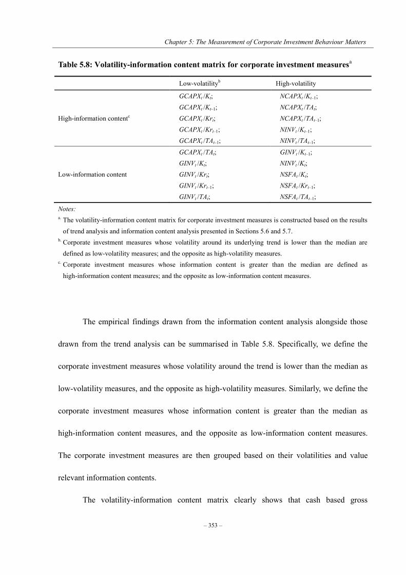
Chapter 5: The Measurement of Corporate Investment Behaviour Matters
– 353 –
Table 5.8: Volatility-information content matrix for corporate investment measuresa
Notes: a. The volatility-information content matrix for corporate investment measures is constructed based on the results
of trend analysis and information content analysis presented in Sections 5.6 and 5.7. b. Corporate investment measures whose volatility around its underlying trend is lower than the median are
defined as low-volatility measures; and the opposite as high-volatility measures. c. Corporate investment measures whose information content is greater than the median are defined as
high-information content measures; and the opposite as low-information content measures.
The empirical findings drawn from the information content analysis alongside those
drawn from the trend analysis can be summarised in Table 5.8. Specifically, we define the
corporate investment measures whose volatility around the trend is lower than the median as
low-volatility measures, and the opposite as high-volatility measures. Similarly, we define the
corporate investment measures whose information content is greater than the median as
high-information content measures, and the opposite as low-information content measures.
The corporate investment measures are then grouped based on their volatilities and value
relevant information contents.
The volatility-information content matrix clearly shows that cash based gross
Low-volatilityb High-volatility
High-information contentc
GCAPXt /Kt; GCAPXt /Kt–1; GCAPXt /Krt; GCAPXt /Krt–1; GCAPXt /TAt–1;
NCAPXt /Kt–1; NCAPXt /TAt; NCAPXt /TAt–1; NINVt /Kt–1; NINVt /TAt–1;
Low-information content
GCAPXt /TAt; GINVt /Kt; GINVt /Krt; GINVt /Krt–1; GINVt /TAt;
GINVt /Kt–1; NINVt /Kt; NSFAt /Kt; NSFAt /Krt–1; NSFAt /TAt–1;
Chapter 5: The Measurement of Corporate Investment Behaviour Matters
– 354 –
corporate investment measures, except GCAPXt /TAt, contain less noise and provide greater
value relevant information, and thus are the best performing measures among the alternatives.
Both cash based and accrual based net corporate investment measures, excluding NINVt /Kt,
are also rather informative, but they exhibit relatively high levels of volatility around their
respective underlying trends, which makes them noisy and less predictable. In contrast,
accrual based gross corporate investment measures, with the exception of GINVt /Kt–1, are
found to be less volatile and thus more predictable. However, they are relatively less relevant
to company value, and hence less useful in explaining variations in company value. Besides,
cash based net spending on fixed assets measures are without exception characterised by high
volatility and low information content, therefore are less attractive compared to the
alternatives.
5.8 Concluding remarks
The use of corporate investment to capital stock ratio as a measure of corporate investment
behaviour has been common practice in empirical analyses. Although the corporate
investment measures are similarly constructed, they in fact vary both in terms of the
numerator and the denominator. However, no attempt has been made to provide a comparison
among various corporate investment measures. One claim which has been implicitly made is
that different measures of corporate investment behaviour will always yield the same, or at
least qualitatively similar, results in empirical analyses. As a consequence, we know little
about how differently these corporate investment measures perform in empirical analyses, and
Chapter 5: The Measurement of Corporate Investment Behaviour Matters
– 355 –
the extent to which the choice of corporate investment measures may influence the
conclusions drawn from empirical analyses. This chapter, therefore, aims to fill these gaps by
offering the first attempt to discriminate conceptually and evaluate empirically twenty
different corporate investment measures which are currently used in the literature.
We first discriminate various corporate investment measures from an accounting
perspective. Given the fact that different accounting principles as well as different elements
are involved in the preparation of relevant accounting items used to construct the corporate
investment measures, corporate investment to capital stock ratios with different specifications
are likely to carry different sets of information about a company’s investing activities. Due to
a lack of understanding of the financial information provided by the relevant accounting items,
corporate investment measures are potentially misused in empirical analyses of corporate
investment behaviour. The conflicting conclusions drawn from the existing literature on
corporate investment, therefore, may also be attributable to the differences in measuring
companies’ investment behaviour.
Based on a balanced panel of UK-listed companies over the period 1999–2008, it is
found that the corporate investment measures with different specifications are not uniformly
positively correlated with one another. Significantly negative correlations are also observed
among the alternatives, which appear surprising since they are supposed to measure the
investment behaviour of the same batch of companies over the same period of time. Therefore,
we argue that the choice of corporate investment measures is likely to have a profound impact
Chapter 5: The Measurement of Corporate Investment Behaviour Matters
– 356 –
on the conclusions drawn from the empirical analyses of corporate investment behaviour. Our
argument is empirically supported by the results obtained from estimating a simple Tobin’s Q
model. As expected, distinct conclusions with respect to the association between Tobin’s Q
and companies’ investment behaviour can be drawn when different corporate investment
measures are employed as the dependent variable, indicating that the measurement of
corporate investment behaviour does indeed matter in empirical analyses.
To evaluate the empirical performance of the alternative corporate investment
measures, we carry out both trend analysis and information content analysis. The trend
analysis results suggest that the gross investment measures are systematically less volatile
around their respective trends, and thus are less noisy compared to the net investment
measures. The excess volatility of net investment measures is largely due to the noise
contained in the depreciation component which is potentially subject to managerial
manipulation. Meanwhile, the information content analysis results show that cash based
corporate investment measures are systematically more informative than their accrual based
counterparts, suggesting that investors are more concerned with cash flow based measures
which are less likely to be distorted by the choices of discretionary accounting policies and by
managers’ opportunistic manipulations as compared to the accrual based measures.
According to the results from both analyses, we conclude that cash based gross
corporate investment to capital stock ratios are the best performing measures of corporate
investments behaviour among the alternatives, as they contain relatively less noise and greater

Chapter 5: The Measurement of Corporate Investment Behaviour Matters
– 357 –
value relevant information. Researchers in the area of corporate finance, therefore, are
suggested to utilise cash based gross corporate investment measures for their future empirical
analyses if they have to make mutually exclusive choices among the alternatives without any
particular preference. Overall, this chapter may shed some light and provide some guidance
for measuring corporate investment behaviour.

Chapter 5: The Measurement of Corporate Investment Behaviour Matters
– 358 –
Appendix 5.A: Perpetual inventory method for estimating the replacement value of capital stock
Replacement value of capital stock (Kr) used in this chapter is calculated on the basis on the standard perpetual
inventory formula developed by Salinger and Summers (1983). Specifically, we treat book value of net property,
plant and equipment (NPPE) as historic value of capital stock, and assume that replacement value and historic
value are the same in the first year of data for each company. We then apply the perpetual inventory formula as
follows:
it
ititit DDA
INVGPPEL
1 (5A.1)
)/21()( 11
iitt
titit LKr
pp
INVKr
(5A.2)
where Lit represents the useful life of company i’s capital goods in year t; GPPEt–1 represents book value of gross
property, plant and equipment at the beginning of year t; INVt represents corporate investment in year t; DDAt
represents accounting depreciation, depletion and amortization in year t; Kr represents the replacement value of
capital stock; and pt represents the price of investment goods, which is proxied by the implicit deflator for gross
fixed capital formation obtained from UK Office for National Statistics (ONS). Since Lit fluctuates from year to
year, we use Li which is an average of Lit over time as a proxy for the useful life of company i’s capital goods.
The amount of the capital stock depreciated each year is calculated based on the assumption that economic
depreciation is double declining balance (this may result in negative replacement value of capital stock). See
Salinger and Summer (1983) for the other assumptions necessary to use this method of calculation.
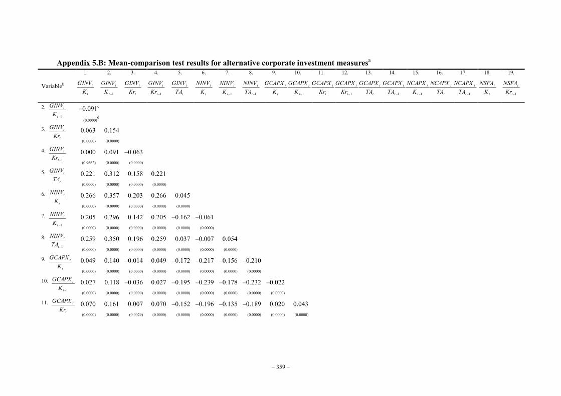
– 359 –
Appendix 5.B: Mean-comparison test results for alternative corporate investment measuresa
Variableb
1.
t
t
KGINV
2.
1t
t
KGINV
3.
t
t
KrGINV
4.
1t
t
KrGINV
5.
t
t
TAGINV
6.
t
t
KNINV
7.
1t
t
KNINV
8.
1t
t
TANINV
9.
t
t
KGCAPX
10.
1t
t
KGCAPX
11.
t
t
KrGCAPX
12.
1t
t
KrGCAPX
13.
t
t
TAGCAPX
14.
1t
t
TAGCAPX
15.
1t
t
KNCAPX
16.
t
t
TANCAPX
17.
1t
t
TANCAPX
18.
t
t
KNSFA
19.
1t
t
KrNSFA
2. 1t
t
KGINV
–0.091c (0.0000)
d
3. t
t
KrGINV
0.063 (0.0000)
0.154 (0.0000)
4. 1t
t
KrGINV
0.000 (0.9662)
0.091 (0.0000)
–0.063 (0.0000)
5. t
t
TAGINV
0.221 (0.0000)
0.312 (0.0000)
0.158 (0.0000)
0.221 (0.0000)
6. t
t
KNINV
0.266 (0.0000)
0.357 (0.0000)
0.203 (0.0000)
0.266 (0.0000)
0.045 (0.0000)
7. 1t
t
KNINV
0.205 (0.0000)
0.296 (0.0000)
0.142 (0.0000)
0.205 (0.0000)
–0.162 (0.0000)
–0.061 (0.0000)
8. 1t
t
TANINV
0.259 (0.0000)
0.350 (0.0000)
0.196 (0.0000)
0.259 (0.0000)
0.037 (0.0000)
–0.007 (0.0000)
0.054 (0.0000)
9. t
t
KGCAPX
0.049 (0.0000)
0.140 (0.0000)
–0.014 (0.0000)
0.049 (0.0000)
–0.172 (0.0000)
–0.217 (0.0000)
–0.156 (0.0000)
–0.210 (0.0000)
10. 1t
t
KGCAPX
0.027 (0.0000)
0.118 (0.0000)
–0.036 (0.0000)
0.027 (0.0000)
–0.195 (0.0000)
–0.239 (0.0000)
–0.178 (0.0000)
–0.232 (0.0000)
–0.022 (0.0000)
11. t
t
KrGCAPX
0.070 (0.0000)
0.161 (0.0000)
0.007 (0.0029)
0.070 (0.0000)
–0.152 (0.0000)
–0.196 (0.0000)
–0.135 (0.0000)
–0.189 (0.0000)
0.020 (0.0000)
0.043 (0.0000)
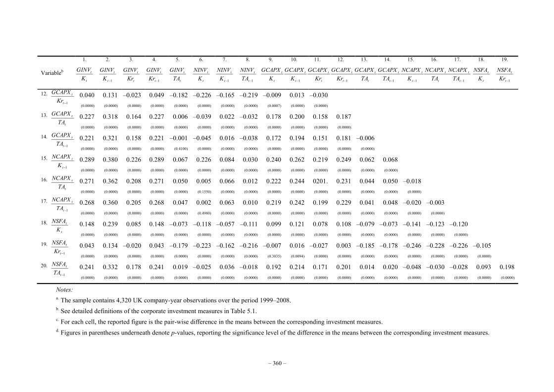
– 360 –
Variableb
1.
t
t
KGINV
2.
1t
t
KGINV
3.
t
t
KrGINV
4.
1t
t
KrGINV
5.
t
t
TAGINV
6.
t
t
KNINV
7.
1t
t
KNINV
8.
1t
t
TANINV
9.
t
t
KGCAPX
10.
1t
t
KGCAPX
11.
t
t
KrGCAPX
12.
1t
t
KrGCAPX
13.
t
t
TAGCAPX
14.
1t
t
TAGCAPX
15.
1t
t
KNCAPX
16.
t
t
TANCAPX
17.
1t
t
TANCAPX
18.
t
t
KNSFA
19.
1t
t
KrNSFA
12. 1t
t
KrGCAPX
0.040 (0.0000)
0.131 (0.0000)
–0.023 (0.0000)
0.049 (0.0000)
–0.182 (0.0000)
–0.226 (0.0000)
–0.165 (0.0000)
–0.219 (0.0000)
–0.009 (0.0007)
0.013 (0.0000)
–0.030 (0.0000)
13. t
t
TAGCAPX
0.227 (0.0000)
0.318 (0.0000)
0.164 (0.0000)
0.227 (0.0000)
0.006 (0.0000)
–0.039 (0.0000)
0.022 (0.0000)
–0.032 (0.0000)
0.178 (0.0000)
0.200 (0.0000)
0.158 (0.0000)
0.187 (0.0000)
14. 1t
t
TAGCAPX
0.221 (0.0000)
0.321 (0.0000)
0.158 (0.0000)
0.221 (0.0000)
–0.001 (0.4100)
–0.045 (0.0000)
0.016 (0.0000)
–0.038 (0.0000)
0.172 (0.0000)
0.194 (0.0000)
0.151 (0.0000)
0.181 (0.0000)
–0.006 (0.0000)
15. 1t
t
KNCAPX
0.289 (0.0000)
0.380 (0.0000)
0.226 (0.0000)
0.289 (0.0000)
0.067 (0.0000)
0.226 (0.0000)
0.084 (0.0000)
0.030 (0.0000)
0.240 (0.0000)
0.262 (0.0000)
0.219 (0.0000)
0.249 (0.0000)
0.062 (0.0000)
0.068 (0.0000)
16. t
t
TANCAPX
0.271 (0.0000)
0.362 (0.0000)
0.208 (0.0000)
0.271 (0.0000)
0.050 (0.0000)
0.005 (0.1550)
0.066 (0.0000)
0.012 (0.0000)
0.222 (0.0000)
0.244 (0.0000)
0201. (0.0000)
0.231 (0.0000)
0.044 (0.0000)
0.050 (0.0000)
–0.018 (0.0000)
17. 1t
t
TANCAPX
0.268 (0.0000)
0.360 (0.0000)
0.205 (0.0000)
0.268 (0.0000)
0.047 (0.0000)
0.002 (0.4980)
0.063 (0.0000)
0.010 (0.0000)
0.219 (0.0000)
0.242 (0.0000)
0.199 (0.0000)
0.229 (0.0000)
0.041 (0.0000)
0.048 (0.0000)
–0.020 (0.0000)
–0.003 (0.0000)
18. t
t
KNSFA
0.148 (0.0000)
0.239 (0.0000)
0.085 (0.0000)
0.148 (0.0000)
–0.073 (0.0000)
–0.118 (0.0000)
–0.057 (0.0000)
–0.111 (0.0000)
0.099 (0.0000)
0.121 (0.0000)
0.078 (0.0000)
0.108 (0.0000)
–0.079 (0.0000)
–0.073 (0.0000)
–0.141 (0.0000)
–0.123 (0.0000)
–0.120 (0.0000)
19. 1t
t
KrNSFA
0.043 (0.0000)
0.134 (0.0000)
–0.020 (0.0000)
0.043 (0.0000)
–0.179 (0.0000)
–0.223 (0.0000)
–0.162 (0.0000)
–0.216 (0.0000)
–0.007 (0.3035)
0.016 (0.0094)
–0.027 (0.0000)
0.003 (0.0000)
–0.185 (0.0000)
–0.178 (0.0000)
–0.246 (0.0000)
–0.228 (0.0000)
–0.226 (0.0000)
–0.105 (0.0000)
20. 1t
t
TANSFA
0.241 (0.0000)
0.332 (0.0000)
0.178 (0.0000)
0.241 (0.0000)
0.019 (0.0000)
–0.025 (0.0000)
0.036 (0.0000)
–0.018 (0.0000)
0.192 (0.0000)
0.214 (0.0000)
0.171 (0.0000)
0.201 (0.0000)
0.014 (0.0000)
0.020 (0.0000)
–0.048 (0.0000)
–0.030 (0.0000)
–0.028 (0.0000)
0.093 (0.0000)
0.198 (0.0000)
Notes: a. The sample contains 4,320 UK company-year observations over the period 1999–2008. b. See detailed definitions of the corporate investment measures in Table 5.1. c. For each cell, the reported figure is the pair-wise difference in the means between the corresponding investment measures. d. Figures in parentheses underneath denote p-values, reporting the significance level of the difference in the means between the corresponding investment measures.
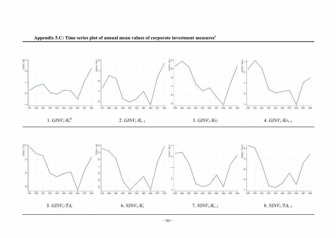
– 361 –
Appendix 5.C: Time series plot of annual mean values of corporate investment measuresa
1. GINVt /Ktb 2. GINVt /Kt–1 3. GINVt /Krt 4. GINVt /Krt–1
5. GINVt /TAt 6. NINVt /Kt 7. NINVt /Kt–1 8. NINVt /TAt–1
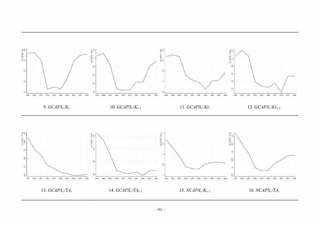
– 362 –
9. GCAPXt /Kt 10. GCAPXt /Kt–1 11. GCAPXt /Krt 12. GCAPXt /Krt–1
13. GCAPXt /TAt 14. GCAPXt /TAt–1 15. NCAPXt /Kt–1 16. NCAPXt /TAt
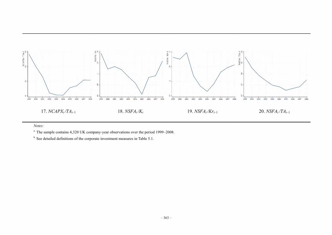
– 363 –
17. NCAPXt /TAt–1 18. NSFAt /Kt 19. NSFAt /Krt–1 20. NSFAt /TAt–1
Notes: a. The sample contains 4,320 UK company-year observations over the period 1999–2008. b. See detailed definitions of the corporate investment measures in Table 5.1.
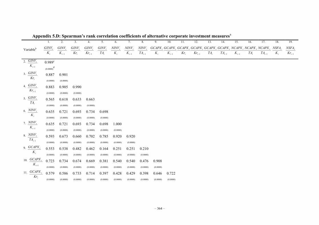
– 364 –
Appendix 5.D: Spearman’s rank correlation coefficients of alternative corporate investment measuresa
Variableb
1.
t
t
KGINV
2.
1t
t
KGINV
3.
t
t
KrGINV
4.
1t
t
KrGINV
5.
t
t
TAGINV
6.
t
t
KNINV
7.
1t
t
KNINV
8.
1t
t
TANINV
9.
t
t
KGCAPX
10.
1t
t
KGCAPX
11.
t
t
KrGCAPX
12.
1t
t
KrGCAPX
13.
t
t
TAGCAPX
14.
1t
t
TAGCAPX
15.
1t
t
KNCAPX
16.
t
t
TANCAPX
17.
1t
t
TANCAPX
18.
t
t
KNSFA
19.
1t
t
KrNSFA
2. 1t
t
KGINV
0.989c (0.0000)
d
3. t
t
KrGINV
0.887 (0.0000)
0.901 (0.0000)
4. 1t
t
KrGINV
0.883 (0.0000)
0.905 (0.0000)
0.990 (0.0000)
5. t
t
TAGINV
0.565 (0.0000)
0.618 (0.0000)
0.633 (0.0000)
0.663 (0.0000)
6. t
t
KNINV
0.635 (0.0000)
0.721 (0.0000)
0.693 (0.0000)
0.734 (0.0000)
0.698 (0.0000)
7. 1t
t
KNINV
0.635 (0.0000)
0.721 (0.0000)
0.693 (0.0000)
0.734 (0.0000)
0.698 (0.0000)
1.000 (0.0000)
8. 1t
t
TANINV
0.593 (0.0000)
0.673 (0.0000)
0.660 (0.0000)
0.702 (0.0000)
0.785 (0.0000)
0.920 (0.0000)
0.920 (0.0000)
9. t
t
KGCAPX
0.553 (0.0000)
0.538 (0.0000)
0.482 (0.0000)
0.462 (0.0000)
0.164 (0.0000)
0.251 (0.0000)
0.251 (0.0000)
0.210 (0.0000)
10. 1t
t
KGCAPX
0.723 (0.0000)
0.734 (0.0000)
0.674 (0.0000)
0.669 (0.0000)
0.381 (0.0000)
0.540 (0.0000)
0.540 (0.0000)
0.476 (0.0000)
0.908 (0.0000)
11. t
t
KrGCAPX
0.579 (0.0000)
0.586 (0.0000)
0.733 (0.0000)
0.714 (0.0000)
0.397 (0.0000)
0.428 (0.0000)
0.429 (0.0000)
0.398 (0.0000)
0.646 (0.0000)
0.722 (0.0000)
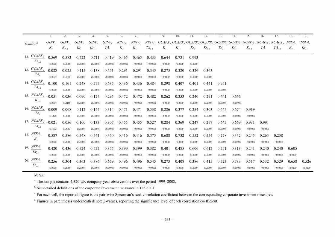
– 365 –
Variableb
1.
t
t
KGINV
2.
1t
t
KGINV
3.
t
t
KrGINV
4.
1t
t
KrGINV
5.
t
t
TAGINV
6.
t
t
KNINV
7.
1t
t
KNINV
8.
1t
t
TANINV
9.
t
t
KGCAPX
10.
1t
t
KGCAPX
11.
t
t
KrGCAPX
12.
1t
t
KrGCAPX
13.
t
t
TAGCAPX
14.
1t
t
TAGCAPX
15.
1t
t
KNCAPX
16.
t
t
TANCAPX
17.
1t
t
TANCAPX
18.
t
t
KNSFA
19.
1t
t
KrNSFA
12. 1t
t
KrGCAPX
0.569 (0.0000)
0.583 (0.0000)
0.722 (0.0000)
0.711 (0.0000)
0.419 (0.0000)
0.465 (0.0000)
0.465 (0.0000)
0.433 (0.0000)
0.644 (0.0000)
0.731 (0.0000)
0.993 (0.0000)
13. t
t
TAGCAPX
–0.028 (0.0677)
0.025 (0.1016)
0.115 (0.0000)
0.138 (0.0000)
0.561 (0.0000)
0.291 (0.0000)
0.291 (0.0000)
0.345 (0.0000)
0.275 (0.0000)
0.320 (0.0000)
0.326 (0.0000)
0.363 (0.0000)
14. 1t
t
TAGCAPX
0.100 (0.0000)
0.161 (0.0000)
0.248 (0.0000)
0.275 (0.0000)
0.635 (0.0000)
0.436 (0.0000)
0.436 (0.0000)
0.484 (0.0000)
0.298 (0.0000)
0.407 (0.0000)
0.401 (0.0000)
0.441 (0.0000)
0.951 (0.0000)
15. 1t
t
KNCAPX
–0.051 (0.0007)
0.036 (0.0188)
0.090 (0.0000)
0.124 (0.0000)
0.295 (0.0000)
0.472 (0.0000)
0.472 (0.0000)
0.482 (0.0000)
0.262 (0.0000)
0.353 (0.0000)
0.240 (0.0000)
0.291 (0.0000)
0.641 (0.0000)
0.666 (0.0000)
16. t
t
TANCAPX
–0.009 (0.5428)
0.068 (0.0000)
0.112 (0.0000)
0.144 (0.0000)
0.314 (0.0000)
0.471 (0.0000)
0.471 (0.0000)
0.538 (0.0000)
0.286 (0.0000)
0.377 (0.0000)
0.254 (0.0000)
0.303 (0.0000)
0.645 (0.0000)
0.674 (0.0000)
0.919 (0.0000)
17. 1t
t
TANCAPX
–0.021 (0.1692)
0.056 (0.0002)
0.100 (0.0000)
0.133 (0.0000)
0.307 (0.0000)
0.455 (0.0000)
0.455 (0.0000)
0.527 (0.0000)
0.284 (0.0000)
0.369 (0.0000)
0.247 (0.0000)
0.297 (0.0000)
0.645 (0.0000)
0.669 (0.0000)
0.931 (0.0000)
0.991 (0.0000)
18. t
t
KNSFA
0.587 (0.0000)
0.586 (0.0000)
0.548 (0.0000)
0.541 (0.0000)
0.360 (0.0000)
0.416 (0.0000)
0.416 (0.0000)
0.375 (0.0000)
0.688 (0.0000)
0.732 (0.0000)
0.552 (0.0000)
0.554 (0.0000)
0.278 (0.0000)
0.332 (0.0000)
0.245 (0.0000)
0.263 (0.0000)
0.258 (0.0000)
19. 1t
t
KrNSFA
0.420 (0.0000)
0.436 (0.0000)
0.524 (0.0000)
0.522 (0.0000)
0.355 (0.0000)
0.399 (0.0000)
0.399 (0.0000)
0.382 (0.0000)
0.401 (0.0000)
0.485 (0.0000)
0.606 (0.0000)
0.612 (0.0000)
0.251 (0.0000)
0.313 (0.0000)
0.241 (0.0000)
0.240 (0.0000)
0.240 (0.0000)
0.605 (0.0000)
20. 1t
t
TANSFA
0.256 (0.0000)
0.304 (0.0000)
0.363 (0.0000)
0.386 (0.0000)
0.659 (0.0000)
0.496 (0.0000)
0.496 (0.0000)
0.545 (0.0000)
0.273 (0.0000)
0.408 (0.0000)
0.386 (0.0000)
0.415 (0.0000)
0.723 (0.0000)
0.783 (0.0000)
0.517 (0.0000)
0.532 (0.0000)
0.529 (0.0000)
0.658 (0.0000)
0.526 (0.0000)
Notes: a. The sample contains 4,320 UK company-year observations over the period 1999–2008. b. See detailed definitions of the corporate investment measures in Table 5.1. c. For each cell, the reported figure is the pair-wise Spearman’s rank correlation coefficient between the corresponding corporate investment measures. d. Figures in parentheses underneath denote p-values, reporting the significance level of each correlation coefficient.
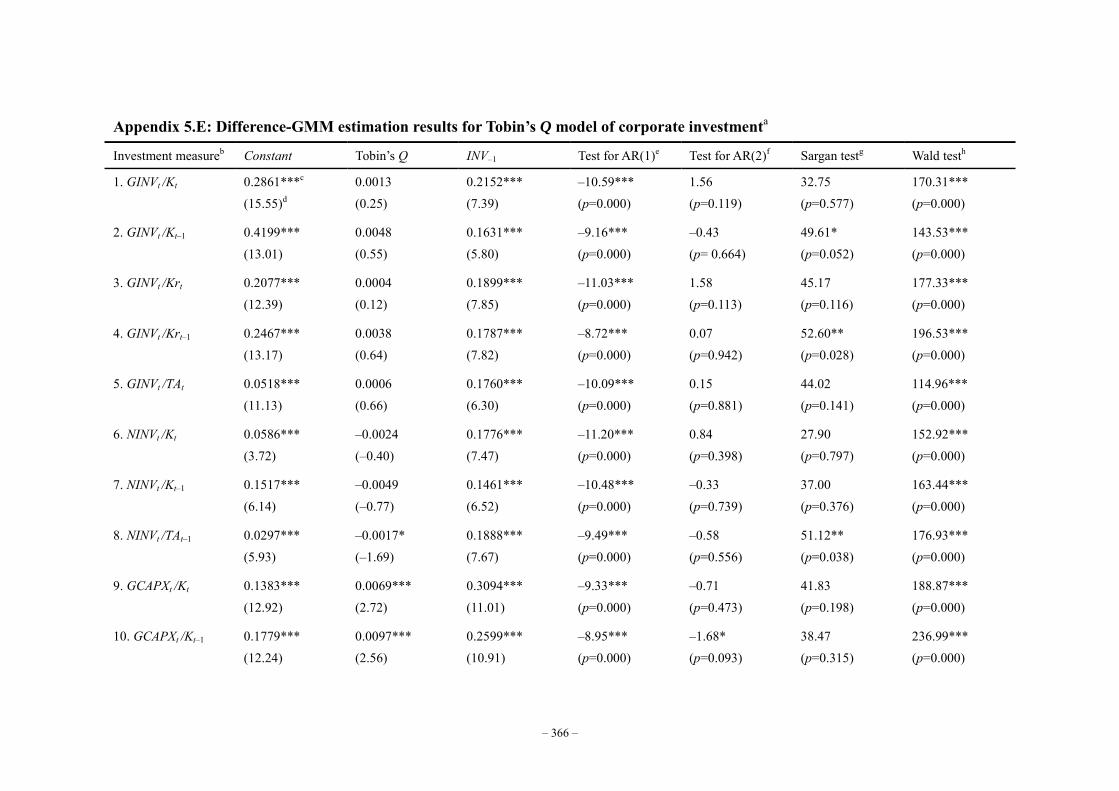
– 366 –
Appendix 5.E: Difference-GMM estimation results for Tobin’s Q model of corporate investmenta
Investment measureb Constant Tobin’s Q INV–1 Test for AR(1)e Test for AR(2)f Sargan testg Wald testh
1. GINVt /Kt 0.2861***c (15.55)d
0.0013 (0.25)
0.2152*** (7.39)
–10.59*** (p=0.000)
1.56 (p=0.119)
32.75 (p=0.577)
170.31*** (p=0.000)
2. GINVt /Kt–1 0.4199*** (13.01)
0.0048 (0.55)
0.1631*** (5.80)
–9.16*** (p=0.000)
–0.43 (p= 0.664)
49.61* (p=0.052)
143.53*** (p=0.000)
3. GINVt /Krt 0.2077*** (12.39)
0.0004 (0.12)
0.1899*** (7.85)
–11.03*** (p=0.000)
1.58 (p=0.113)
45.17 (p=0.116)
177.33*** (p=0.000)
4. GINVt /Krt–1 0.2467*** (13.17)
0.0038 (0.64)
0.1787*** (7.82)
–8.72*** (p=0.000)
0.07 (p=0.942)
52.60** (p=0.028)
196.53*** (p=0.000)
5. GINVt /TAt 0.0518*** (11.13)
0.0006 (0.66)
0.1760*** (6.30)
–10.09*** (p=0.000)
0.15 (p=0.881)
44.02 (p=0.141)
114.96*** (p=0.000)
6. NINVt /Kt 0.0586*** (3.72)
–0.0024 (–0.40)
0.1776*** (7.47)
–11.20*** (p=0.000)
0.84 (p=0.398)
27.90 (p=0.797)
152.92*** (p=0.000)
7. NINVt /Kt–1 0.1517*** (6.14)
–0.0049 (–0.77)
0.1461*** (6.52)
–10.48*** (p=0.000)
–0.33 (p=0.739)
37.00 (p=0.376)
163.44*** (p=0.000)
8. NINVt /TAt–1 0.0297*** (5.93)
–0.0017* (–1.69)
0.1888*** (7.67)
–9.49*** (p=0.000)
–0.58 (p=0.556)
51.12** (p=0.038)
176.93*** (p=0.000)
9. GCAPXt /Kt 0.1383*** (12.92)
0.0069*** (2.72)
0.3094*** (11.01)
–9.33*** (p=0.000)
–0.71 (p=0.473)
41.83 (p=0.198)
188.87*** (p=0.000)
10. GCAPXt /Kt–1 0.1779*** (12.24)
0.0097*** (2.56)
0.2599*** (10.91)
–8.95*** (p=0.000)
–1.68* (p=0.093)
38.47 (p=0.315)
236.99*** (p=0.000)
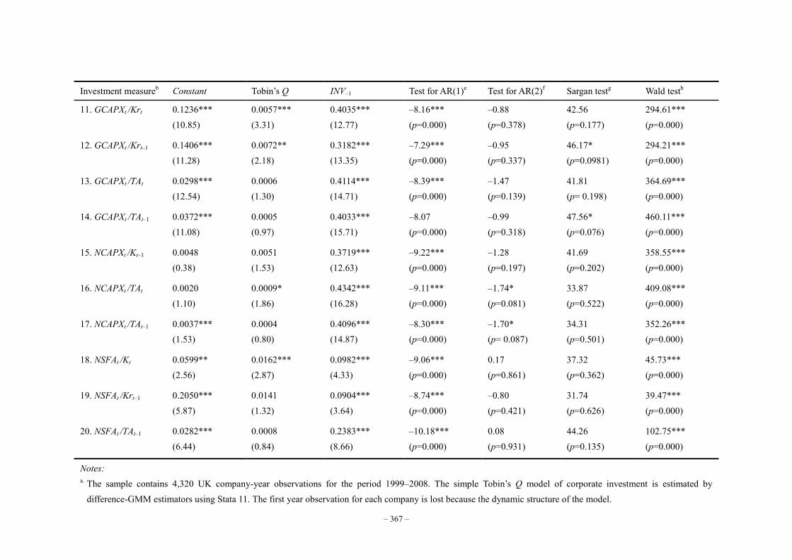
– 367 –
Investment measureb Constant Tobin’s Q INV–1 Test for AR(1)e Test for AR(2)f Sargan testg Wald testh
11. GCAPXt /Krt 0.1236*** (10.85)
0.0057*** (3.31)
0.4035*** (12.77)
–8.16*** (p=0.000)
–0.88 (p=0.378)
42.56 (p=0.177)
294.61*** (p=0.000)
12. GCAPXt /Krt–1 0.1406*** (11.28)
0.0072** (2.18)
0.3182*** (13.35)
–7.29*** (p=0.000)
–0.95 (p=0.337)
46.17* (p=0.0981)
294.21*** (p=0.000)
13. GCAPXt /TAt 0.0298*** (12.54)
0.0006 (1.30)
0.4114*** (14.71)
–8.39*** (p=0.000)
–1.47 (p=0.139)
41.81 (p= 0.198)
364.69*** (p=0.000)
14. GCAPXt /TAt–1 0.0372*** (11.08)
0.0005 (0.97)
0.4033*** (15.71)
–8.07 (p=0.000)
–0.99 (p=0.318)
47.56* (p=0.076)
460.11*** (p=0.000)
15. NCAPXt /Kt–1 0.0048 (0.38)
0.0051 (1.53)
0.3719*** (12.63)
–9.22*** (p=0.000)
–1.28 (p=0.197)
41.69 (p=0.202)
358.55*** (p=0.000)
16. NCAPXt /TAt 0.0020 (1.10)
0.0009* (1.86)
0.4342*** (16.28)
–9.11*** (p=0.000)
–1.74* (p=0.081)
33.87 (p=0.522)
409.08*** (p=0.000)
17. NCAPXt /TAt–1 0.0037*** (1.53)
0.0004 (0.80)
0.4096*** (14.87)
–8.30*** (p=0.000)
–1.70* (p= 0.087)
34.31 (p=0.501)
352.26*** (p=0.000)
18. NSFAt /Kt 0.0599** (2.56)
0.0162*** (2.87)
0.0982*** (4.33)
–9.06*** (p=0.000)
0.17 (p=0.861)
37.32 (p=0.362)
45.73*** (p=0.000)
19. NSFAt /Krt–1 0.2050*** (5.87)
0.0141 (1.32)
0.0904*** (3.64)
–8.74*** (p=0.000)
–0.80 (p=0.421)
31.74 (p=0.626)
39.47*** (p=0.000)
20. NSFAt /TAt–1 0.0282*** (6.44)
0.0008 (0.84)
0.2383*** (8.66)
–10.18*** (p=0.000)
0.08 (p=0.931)
44.26 (p=0.135)
102.75*** (p=0.000)
Notes: a. The sample contains 4,320 UK company-year observations for the period 1999–2008. The simple Tobin’s Q model of corporate investment is estimated by
difference-GMM estimators using Stata 11. The first year observation for each company is lost because the dynamic structure of the model.

– 368 –
b. Different corporate investment measures are used as the dependent variable (INV) in their respective regressions. The Tobin’s Q model is specified as
itititit INVQINV 1210
We also control for time effects by adding a set of year dummy variables. The instruments used for the regression include Constant, ∆Year dummies, ∆Qt, and INVt-2….
c. * significant at the 10% level; ** significant at the 5% level; and *** significant at the 1% level. d. t-statistics are reported in parentheses. e. The Arellona-Bond test tests for serial correlation in the first-differenced errors in order to purge the unobserved and perfectly autocorrelated individual effects.
Autocorrelation at order 1 is expected in first differences, because 1 ititit should correlate with 211 ititit , since they share the 1it term. f. To check for AR(1) in levels, look for AR(2) in differences, in the idea that this will detect the relationship between the 1it in it and the 2it in 2 it .
Autocorrelation indicates that lags of the dependent variable (and any other variables used as instruments that are not strictly exogenous), are in fact endogenous, thus bad instruments. Therefore, rejecting the null hypothesis of no serial correlation in the first-differenced errors at an order greater than one implies model misspecification.
g. The Sargan overidentifying restrictions test tests for whether the instruments, as a group, appear exogenous. The joint null hypothesis is that the instruments are valid instruments, i.e. uncorrelated with the error term, and that the excluded instruments are correctly excluded from the estimated equation. A statistically significant test statistic always indicates that the instruments may not be valid. Under the null hypothesis of instrument validity, the Sargan test has an asymptotic Chi-squared distribution.
h. The Wald test tests the null hypothesis that all of the coefficients except the intercept coefficient are jointly zero.
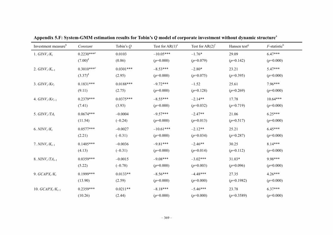
– 369 –
Appendix 5.F: System-GMM estimation results for Tobin’s Q model of corporate investment without dynamic structurea
Investment measureb Constant Tobin’s Q Test for AR(1)e Test for AR(2)f Hansen testg F-statistich
1. GINVt /Kt 0.2230***c (7.00)d
0.0103 (0.86)
–10.05*** (p=0.000)
–1.76* (p=0.079)
29.09 (p=0.142)
6.47*** (p=0.000)
2. GINVt /Kt–1 0.3010***c (3.37)d
0.0301*** (2.95)
–8.53*** (p=0.000)
–2.80* (p=0.075)
23.21 (p=0.395)
5.47*** (p=0.000)
3. GINVt /Krt 0.1831*** (9.11)
0.0188*** (2.75)
–9.72*** (p=0.000)
–1.52 (p=0.128)
25.61 (p=0.269)
7.96*** (p=0.000)
4. GINVt /Krt–1 0.2379*** (7.41)
0.0375*** (3.93)
–8.55*** (p=0.000)
–2.14** (p=0.032)
17.78 (p=0.719)
10.64*** (p=0.000)
5. GINVt /TAt 0.0674*** (11.54)
–0.0004 (–0.24)
–9.57*** (p=0.000)
–2.47** (p=0.013)
21.06 (p=0.517)
6.25*** (p=0.000)
6. NINVt /Kt 0.0577*** (2.21)
–0.0027 (–0.31)
–10.61*** (p=0.000)
–2.12** (p=0.034)
25.21 (p=0.287)
6.45*** (p=0.000)
7. NINVt /Kt–1 0.1405*** (4.13)
–0.0036 (–0.31)
–9.81*** (p=0.000)
–2.46** (p=0.014)
30.25 (p=0.112)
8.14*** (p=0.000)
8. NINVt /TAt–1 0.0359*** (5.22)
–0.0015 (–0.78)
–9.08*** (p=0.000)
–3.02*** (p=0.003)
31.03* (p=0.096)
9.98*** (p=0.000)
9. GCAPXt /Kt 0.1999*** (13.90)
0.0133** (2.59)
–8.56*** (p=0.000)
–4.48*** (p=0.000)
27.35 (p=0.1982)
4.26*** (p=0.000)
10. GCAPXt /Kt–1 0.2359*** (10.26)
0.0211** (2.44)
–8.18*** (p=0.000)
–5.46*** (p=0.000)
23.78 (p=0.3589)
6.37*** (p=0.000)
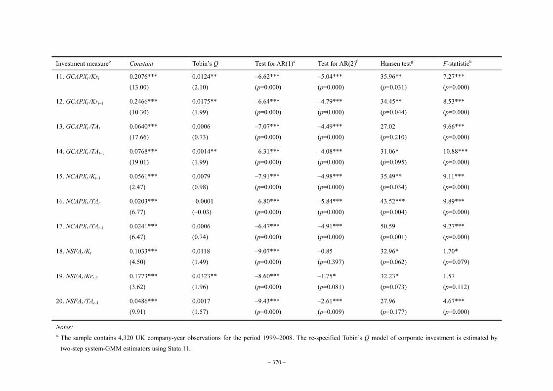
– 370 –
Investment measureb Constant Tobin’s Q Test for AR(1)e Test for AR(2)f Hansen testg F-statistich
11. GCAPXt /Krt 0.2076*** (13.00)
0.0124** (2.10)
–6.62*** (p=0.000)
–5.04*** (p=0.000)
35.96** (p=0.031)
7.27*** (p=0.000)
12. GCAPXt /Krt–1 0.2466*** (10.30)
0.0175** (1.99)
–6.64*** (p=0.000)
–4.79*** (p=0.000)
34.45** (p=0.044)
8.53*** (p=0.000)
13. GCAPXt /TAt 0.0640*** (17.66)
0.0006 (0.73)
–7.07*** (p=0.000)
–4.49*** (p=0.000)
27.02 (p=0.210)
9.66*** (p=0.000)
14. GCAPXt /TAt–1 0.0768*** (19.01)
0.0014** (1.99)
–6.31*** (p=0.000)
–4.08*** (p=0.000)
31.06* (p=0.095)
10.88*** (p=0.000)
15. NCAPXt /Kt–1 0.0561*** (2.47)
0.0079 (0.98)
–7.91*** (p=0.000)
–4.98*** (p=0.000)
35.49** (p=0.034)
9.11*** (p=0.000)
16. NCAPXt /TAt 0.0203*** (6.77)
–0.0001 (–0.03)
–6.80*** (p=0.000)
–5.84*** (p=0.000)
43.52*** (p=0.004)
9.89*** (p=0.000)
17. NCAPXt /TAt–1 0.0241*** (6.47)
0.0006 (0.74)
–6.47*** (p=0.000)
–4.91*** (p=0.000)
50.59 (p=0.001)
9.27*** (p=0.000)
18. NSFAt /Kt 0.1033*** (4.50)
0.0118 (1.49)
–9.07*** (p=0.000)
–0.85 (p=0.397)
32.96* (p=0.062)
1.70* (p=0.079)
19. NSFAt /Krt–1 0.1773*** (3.62)
0.0323** (1.96)
–8.60*** (p=0.000)
–1.75* (p=0.081)
32.23* (p=0.073)
1.57 (p=0.112)
20. NSFAt /TAt–1 0.0486*** (9.91)
0.0017 (1.57)
–9.43*** (p=0.000)
–2.61*** (p=0.009)
27.96 (p=0.177)
4.67*** (p=0.000)
Notes: a. The sample contains 4,320 UK company-year observations for the period 1999–2008. The re-specified Tobin’s Q model of corporate investment is estimated by
two-step system-GMM estimators using Stata 11.

– 371 –
b. Different corporate investment measures are used as the dependent variable (INV) in their respective regressions. The Tobin’s Q model is re-specified as
ititit QINV 10.
We also control for time effects by adding a set of year dummy variables. The instruments used for the regression include Constant, Year dummies, Qt-2, Qt-3, ∆Year dummies, and ∆Qt.
c. * significant at the 10% level; ** significant at the 5% level; and *** significant at the 1% level. d. t-statistics are reported in parentheses. e. The Arellona-Bond test tests for serial correlation in the first-differenced errors in order to purge the unobserved and perfectly autocorrelated individual effects.
Autocorrelation at order 1 is expected in first differences, because 1 ititit should correlate with 211 ititit , since they share the 1it term. f. To check for AR(1) in levels, look for AR(2) in differences, in the idea that this will detect the relationship between the 1it in it and the 2it in 2 it .
Autocorrelation indicates that lags of the dependent variable (and any other variables used as instruments that are not strictly exogenous), are in fact endogenous, thus bad instruments. Therefore, rejecting the null hypothesis of no serial correlation in the first-differenced errors at an order greater than one implies model misspecification.
g. The Hansen overidentifying restrictions test tests for whether the instruments, as a group, appear exogenous. Under two-step robust GMM estimation, the Sargan statistic is not robust to heteroscedasticity or autocorrelation, but the Hensen J-statistic, which is the minimised value of the two-step GMM criterion function, is robust. The joint null hypothesis is that the instruments are valid instruments, i.e. uncorrelated with the error term, and that the excluded instruments are correctly excluded from the estimated equation. A statistically significant test statistic always indicates that the instruments may not be valid. However, the J-test has its own problem: it can be greatly weakened by instrument proliferation.
h. F-statistic for the regression which tests the null hypothesis that all of the coefficients except the intercept coefficient are jointly zero.
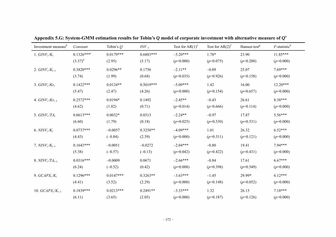
– 372 –
Appendix 5.G: System-GMM estimation results for Tobin’s Q model of corporate investment with alternative measure of Qa
Investment measureb Constant Tobin’s Q INV–1 Test for AR(1)e Test for AR(2)f Hansen testg F-statistich
1. GINVt /Kt 0.1326***c (3.37)d
0.0179*** (2.95)
0.6883*** (5.17)
–5.20*** (p=0.000)
1.78* (p=0.075)
23.90 (p=0.200)
11.85*** (p=0.000)
2. GINVt /Kt–1 0.3820*** (3.74)
0.0296** (1.99)
0.1756 (0.68)
–2.11** (p=0.035)
–0.09 (p=0.926)
25.07 (p=0.158)
7.69*** (p=0.000)
3. GINVt /Krt 0.1422*** (5.47)
0.0124** (2.47)
0.5019*** (4.26)
–5.09*** (p=0.000)
1.42 (p=0.154)
16.00 (p=0.657)
12.20*** (p=0.000)
4. GINVt /Krt–1 0.2572*** (4.62)
0.0194* (1.82)
0.1492 (0.71)
–2.45** (p=0.014)
–0.43 (p=0.666)
26.61 (p=0.114)
8.38*** (p=0.000)
5. GINVt /TAt 0.0613*** (6.60)
0.0032* (1.79)
0.0313 (0.18)
–2.24** (p=0.025)
–0.97 (p=0.330)
17.87 (p=0.531)
5.56*** (p=0.000)
6. NINVt /Kt 0.0737*** (4.43)
–0.0057 (–0.84)
0.3258** (2.39)
–4.09*** (p=0.000)
1.01 (p=0.311)
26.32 (p=0.121)
6.52*** (p=0.000)
7. NINVt /Kt–1 0.1643*** (5.38)
–0.0051 (–0.57)
–0.0272 (–0.13)
–2.04*** (p=0.042)
–0.80 (p=0.422)
19.41 (p=0.431)
7.94*** (p=0.000)
8. NINVt /TAt–1 0.0316*** (6.24)
–0.0009 (–0.52)
0.0671 (0.42)
–2.66*** (p=0.008)
–0.84 (p=0.398)
17.61 (p=0.549)
6.67*** (p=0.000)
9. GCAPXt /Kt 0.1296*** (4.41)
0.0147*** (3.52)
0.3263** (2.29)
–3.63*** (p=0.000)
–1.45 (p=0.148)
29.99* (p=0.052)
6.12*** (p=0.000)
10. GCAPXt /Kt–1 0.1839*** (6.11)
0.0213*** (3.65)
0.2491** (2.05)
–3.53*** (p=0.000)
1.32 (p=0.187)
26.15 (p=0.126)
7.18*** (p=0.000)
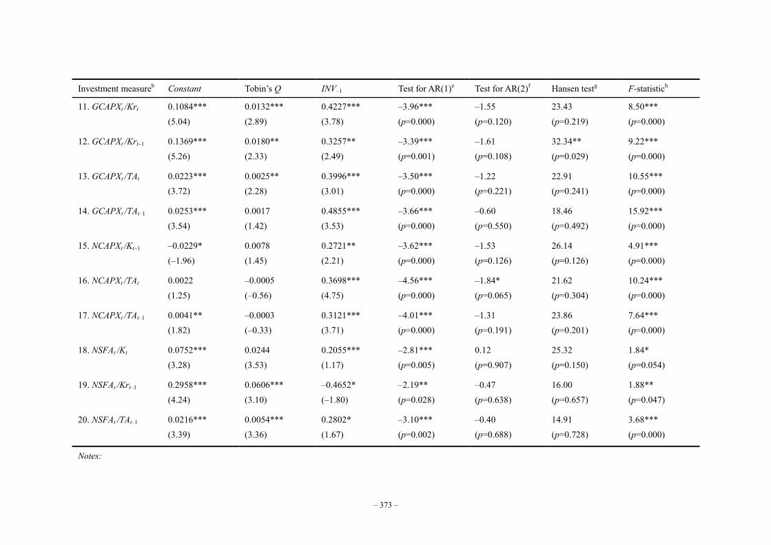
– 373 –
Investment measureb Constant Tobin’s Q INV–1 Test for AR(1)e Test for AR(2)f Hansen testg F-statistich
11. GCAPXt /Krt 0.1084*** (5.04)
0.0132*** (2.89)
0.4227*** (3.78)
–3.96*** (p=0.000)
–1.55 (p=0.120)
23.43 (p=0.219)
8.50*** (p=0.000)
12. GCAPXt /Krt–1 0.1369*** (5.26)
0.0180** (2.33)
0.3257** (2.49)
–3.39*** (p=0.001)
–1.61 (p=0.108)
32.34** (p=0.029)
9.22*** (p=0.000)
13. GCAPXt /TAt 0.0223*** (3.72)
0.0025** (2.28)
0.3996*** (3.01)
–3.50*** (p=0.000)
–1.22 (p=0.221)
22.91 (p=0.241)
10.55*** (p=0.000)
14. GCAPXt /TAt–1 0.0253*** (3.54)
0.0017 (1.42)
0.4855*** (3.53)
–3.66*** (p=0.000)
–0.60 (p=0.550)
18.46 (p=0.492)
15.92*** (p=0.000)
15. NCAPXt /Kt–1 –0.0229* (–1.96)
0.0078 (1.45)
0.2721** (2.21)
–3.62*** (p=0.000)
–1.53 (p=0.126)
26.14 (p=0.126)
4.91*** (p=0.000)
16. NCAPXt /TAt 0.0022 (1.25)
–0.0005 (–0.56)
0.3698*** (4.75)
–4.56*** (p=0.000)
–1.84* (p=0.065)
21.62 (p=0.304)
10.24*** (p=0.000)
17. NCAPXt /TAt–1 0.0041** (1.82)
–0.0003 (–0.33)
0.3121*** (3.71)
–4.01*** (p=0.000)
–1.31 (p=0.191)
23.86 (p=0.201)
7.64*** (p=0.000)
18. NSFAt /Kt 0.0752*** (3.28)
0.0244 (3.53)
0.2055*** (1.17)
–2.81*** (p=0.005)
0.12 (p=0.907)
25.32 (p=0.150)
1.84* (p=0.054)
19. NSFAt /Krt–1 0.2958*** (4.24)
0.0606*** (3.10)
–0.4652* (–1.80)
–2.19** (p=0.028)
–0.47 (p=0.638)
16.00 (p=0.657)
1.88** (p=0.047)
20. NSFAt /TAt–1 0.0216*** (3.39)
0.0054*** (3.36)
0.2802* (1.67)
–3.10*** (p=0.002)
–0.40 (p=0.688)
14.91 (p=0.728)
3.68*** (p=0.000)
Notes:

– 374 –
a. The sample contains 4,320 UK company-year observations for the period 1999–2008. The simple Tobin’s Q model of corporate investment is estimated by two-step system-GMM estimators using Stata 11. Tobin’s Q is measured as the market-to-book value of common equity. The first year observation for each company is lost because the dynamic structure of the model.
b. Different corporate investment measures are used as the dependent variable (INV) in their respective regressions. The Tobin’s Q model is specified as
itititit INVQINV 1210.
We also control for time effects by adding a set of year dummy variables. The instruments used for the regression include Constant, Year dummies, Qt, INVt-3… t-5, ∆Year dummies, ∆Qt and ∆INVt-2.
c. * significant at the 10% level; ** significant at the 5% level; and *** significant at the 1% level. d. t-statistics are reported in parentheses. e. The Arellona-Bond test tests for serial correlation in the first-differenced errors in order to purge the unobserved and perfectly autocorrelated individual effects.
Autocorrelation at order 1 is expected in first differences, because 1 ititit should correlate with 211 ititit , since they share the 1it term. f. To check for AR(1) in levels, look for AR(2) in differences, in the idea that this will detect the relationship between the 1it in it and the 2it in 2 it .
Autocorrelation indicates that lags of the dependent variable (and any other variables used as instruments that are not strictly exogenous), are in fact endogenous, thus bad instruments. Therefore, rejecting the null hypothesis of no serial correlation in the first-differenced errors at an order greater than one implies model misspecification.
g. The Hansen overidentifying restrictions test tests for whether the instruments, as a group, appear exogenous. Under two-step robust GMM estimation, the Sargan statistic is not robust to heteroscedasticity or autocorrelation, but the Hensen J-statistic, which is the minimised value of the two-step GMM criterion function, is robust. The joint null hypothesis is that the instruments are valid instruments, i.e. uncorrelated with the error term, and that the excluded instruments are correctly excluded from the estimated equation. A statistically significant test statistic always indicates that the instruments may not be valid. However, the J-test has its own problem: it can be greatly weakened by instrument proliferation.
h. F-statistic for the regression which tests the null hypothesis that all of the coefficients except the intercept coefficient are jointly zero.
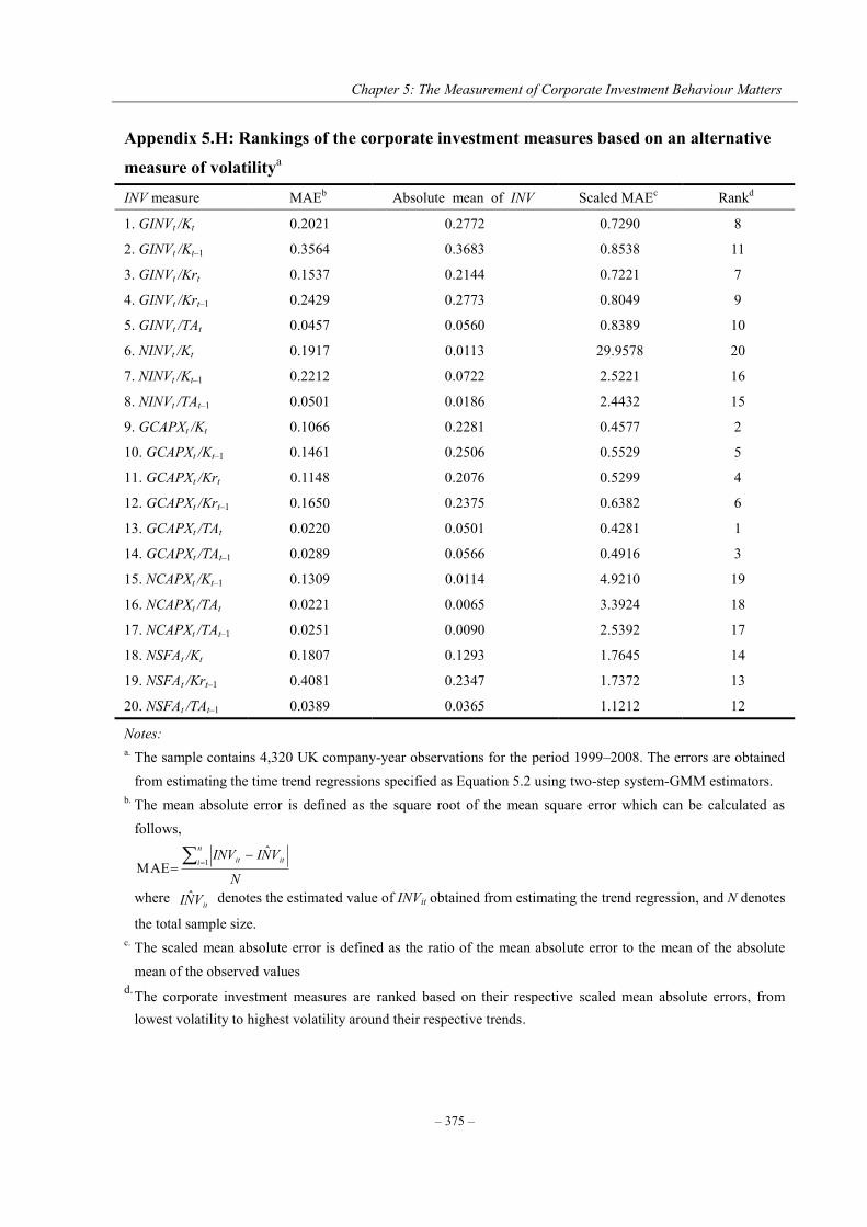
Chapter 5: The Measurement of Corporate Investment Behaviour Matters
– 375 –
Appendix 5.H: Rankings of the corporate investment measures based on an alternative
measure of volatilitya
INV measure MAEb Absolute mean of INV Scaled MAEc Rankd
1. GINVt /Kt 0.2021 0.2772 0.7290 8
2. GINVt /Kt–1 0.3564 0.3683 0.8538 11
3. GINVt /Krt 0.1537 0.2144 0.7221 7
4. GINVt /Krt–1 0.2429 0.2773 0.8049 9
5. GINVt /TAt 0.0457 0.0560 0.8389 10
6. NINVt /Kt 0.1917 0.0113 29.9578 20
7. NINVt /Kt–1 0.2212 0.0722 2.5221 16
8. NINVt /TAt–1 0.0501 0.0186 2.4432 15
9. GCAPXt /Kt 0.1066 0.2281 0.4577 2
10. GCAPXt /Kt–1 0.1461 0.2506 0.5529 5
11. GCAPXt /Krt 0.1148 0.2076 0.5299 4
12. GCAPXt /Krt–1 0.1650 0.2375 0.6382 6
13. GCAPXt /TAt 0.0220 0.0501 0.4281 1
14. GCAPXt /TAt–1 0.0289 0.0566 0.4916 3
15. NCAPXt /Kt–1 0.1309 0.0114 4.9210 19
16. NCAPXt /TAt 0.0221 0.0065 3.3924 18
17. NCAPXt /TAt–1 0.0251 0.0090 2.5392 17
18. NSFAt /Kt 0.1807 0.1293 1.7645 14
19. NSFAt /Krt–1 0.4081 0.2347 1.7372 13
20. NSFAt /TAt–1 0.0389 0.0365 1.1212 12
Notes: a. The sample contains 4,320 UK company-year observations for the period 1999–2008. The errors are obtained
from estimating the time trend regressions specified as Equation 5.2 using two-step system-GMM estimators. b. The mean absolute error is defined as the square root of the mean square error which can be calculated as
follows,
N
VNIINVn
i itit
1
ˆMAE
where itVNI ˆ denotes the estimated value of INVit obtained from estimating the trend regression, and N denotes
the total sample size. c. The scaled mean absolute error is defined as the ratio of the mean absolute error to the mean of the absolute
mean of the observed values d. The corporate investment measures are ranked based on their respective scaled mean absolute errors, from
lowest volatility to highest volatility around their respective trends.
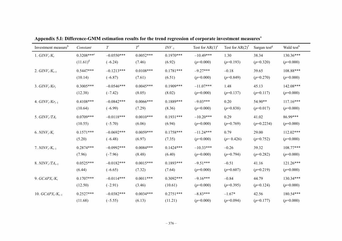
– 376 –
Appendix 5.I: Difference-GMM estimation results for the trend regression of corporate investment measuresa
Investment measureb Constant T T2 INV–1 Test for AR(1)e Test for AR(2)f Sargan testg Wald testh
1. GINVt /Kt 0.3208***c (11.61)d
–0.0550*** (–6.24)
0.0052*** (7.46)
0.1970*** (6.92)
–10.49*** (p=0.000)
1.30 (p=0.193)
38.34 (p=0.320)
130.36*** (p=0.000)
2. GINVt /Kt–1 0.5447*** (10.14)
–0.1213*** (–6.87)
0.0108*** (7.61)
0.1781*** (6.51)
–9.27*** (p=0.000)
–0.18 (p=0.849)
39.65 (p=0.270)
108.88*** (p=0.000)
3. GINVt /Krt 0.3005*** (12.38)
–0.0546*** (–7.42)
0.0045*** (8.05)
0.1909*** (8.02)
–11.07*** (p=0.000)
1.48 (p=0.137)
45.13 (p=0.117)
142.08*** (p=0.000)
4. GINVt /Krt–1 0.4108*** (10.64)
–0.0842*** (–6.99)
0.0066*** (7.29)
0.1889*** (8.36)
–9.03*** (p=0.000)
0.20 (p=0.838)
54.90** (p=0.017)
117.16*** (p=0.000)
5. GINVt /TAt 0.0709*** (10.55)
–0.0118*** (–5.70)
0.0010*** (6.06)
0.1931*** (6.94)
–10.20*** (p=0.000)
0.29 (p=0.769)
41.02 (p=0.2234)
86.99*** (p=0.000)
6. NINVt /Kt 0.1571*** (5.20)
–0.0692*** (–6.48)
0.0059*** (6.97)
0.1758*** (7.35)
–11.24*** (p=0.000)
0.79 (p= 0.426)
29.00 (p=0.752)
112.02*** (p=0.000)
7. NINVt /Kt–1 0.2874*** (7.96)
–0.0992*** (–7.96)
0.0084*** (8.48)
0.1424*** (6.40)
–10.33*** (p=0.000)
–0.26 (p=0.794)
39.32 (p=0.282)
108.77*** (p=0.000)
8. NINVt /TAt–1 0.0525*** (6.44)
–0.0182*** (–6.65)
0.0015*** (7.32)
0.1893*** (7.64)
–9.51*** (p=0.000)
–0.51 (p=0.607)
41.16 (p=0.219)
121.26*** (p=0.000)
9. GCAPXt /Kt 0.1707*** (12.50)
–0.0114*** (–2.91)
0.0011*** (3.46)
0.3092*** (10.61)
–9.16*** (p=0.000)
–0.84 (p=0.395)
44.79 (p=0.124)
130.34*** (p=0.000)
10. GCAPXt /Kt–1 0.2527*** (11.68)
–0.0382*** (–5.55)
0.0034*** (6.13)
0.2751*** (11.21)
–8.83*** (p=0.000)
–1.67* (p=0.094)
42.56 (p=0.177)
180.54*** (p=0.000)
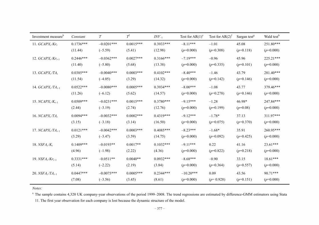
– 377 –
Investment measureb Constant T T2 INV–1 Test for AR(1)e Test for AR(2)f Sargan testg Wald testh
11. GCAPXt /Krt 0.1736*** (11.44)
–0.0201*** (–5.59)
0.0015*** (5.41)
0.3933*** (12.98)
–8.11*** (p=0.000)
–1.01 (p=0.308)
45.08 (p=0.118)
251.80*** (p=0.000)
12. GCAPXt /Krt–1 0.2446*** (11.40)
–0.0362*** (–5.80)
0.0027*** (5.68)
0.3166*** (13.38)
–7.19*** (p=0.000)
–0.96 (p=0.335)
45.96 (p=0.101)
225.21*** (p=0.000)
13. GCAPXt /TAt 0.0385*** (11.54)
–0.0040*** (–4.05)
0.0003*** (3.29)
0.4102*** (14.32)
–8.40*** (p=0.000)
–1.46 (p=0.142)
43.79 (p=0.146)
281.40*** (p=0.000)
14. GCAPXt /TAt–1 0.0522*** (11.26)
–0.0080*** (–6.12)
0.0005*** (5.62)
0.3934*** (14.57)
–8.00*** (p=0.000)
–1.08 (p=0.278)
43.77 (p=0.146)
379.46*** (p=0.000)
15. NCAPXt /Kt–1 0.0509*** (2.44)
–0.0231*** (–3.19)
0.0015*** (2.74)
0.3780*** (12.76)
–9.15*** (p=0.000)
–1.28 (p=0.199)
46.98* (p=0.08)
247.84*** (p=0.000)
16. NCAPXt /TAt 0.0094*** (3.15)
–0.0032*** (–3.18)
0.0002*** (3.14)
0.4319*** (16.50)
–9.12*** (p=0.000)
–1.78* (p=0.075)
37.13 (p=0.370)
311.97*** (p=0.000)
17. NCAPXt /TAt–1 0.0121*** (3.29)
–0.0042*** (–3.47)
0.0003*** (3.59)
0.4085*** (14.75)
–8.23*** (p=0.000)
–1.68* (p=0.092)
35.91 (p=0.425)
260.95*** (p=0.000)
18. NSFAt /Kt 0.1409*** (4.96)
–0.0193** (–1.98)
0.0017** (2.22)
0.1032*** (4.36)
–9.11*** (p=0.000)
0.22 (p=0.822)
41.16 (p=0.218)
23.61*** (p=0.000)
19. NSFAt /Krt–1 0.3331*** (5.14)
–0.0511** (–2.22)
0.0040** (2.19)
0.0932*** (3.84)
–8.68*** (p=0.000)
–0.90 (p=0.364)
33.15 (p=0.557)
18.61*** (p=0.000)
20. NSFAt /TAt–1 0.0447*** (7.08)
–0.0075*** (–3.56)
0.0005*** (3.45)
0.2344*** (8.61)
–10.20*** (p=0.000)
0.09 (p= 0.928)
43.56 (p=0.151)
90.71*** (p=0.000)
Notes: a. The sample contains 4,320 UK company-year observations of the period 1999–2008. The trend regressions are estimated by difference-GMM estimators using Stata
11. The first year observation for each company is lost because the dynamic structure of the model.

– 378 –
b. Different corporate investment measures are used as the dependent variable (INV) in their respective trend regressions. The trend regression is specified as
ititttit INVTTINV 132
210 The instruments used for the regression include Constant, ∆T, ∆T2
t and INVt-2…. c. * significant at the 10% level; ** significant at the 5% level; and *** significant at the 1% level. d. z-statistics are reported in parentheses. e. Arellona-Bond test tests for serial correlation in the first-differenced errors in order to purge the unobserved and perfectly autocorrelated individual effects.
Autocorrelation at order 1 is expected in first differences, because 1 ititit should correlate with 211 ititit , since they share the 1it term. f. To check for AR(1) in levels, look for AR(2) in differences, on the idea that this will detect the relationship between the 1it in it and the 2it in 2 it .
Autocorrelation indicates that lags of the dependent variable (and any other variables used as instruments that are not strictly exogenous), are in fact endogenous, thus bad instruments. Therefore, rejecting the null hypothesis of no serial correlation in the first-differenced errors at an order greater than one implies model misspecification.
g. The Sargan overidentifying restrictions test tests for whether the instruments, as a group, appear exogenous. The joint null hypothesis is that the instruments are valid instruments, i.e. uncorrelated with the error term, and that the excluded instruments are correctly excluded from the estimated equation. A statistically significant test statistic always indicates that the instruments may not be valid. Under the null hypothesis of instrument validity, the Sargan test has an asymptotic Chi-squared distribution.
h. The Wald test tests the null hypothesis that all of the coefficients except the intercept coefficient are jointly zero.
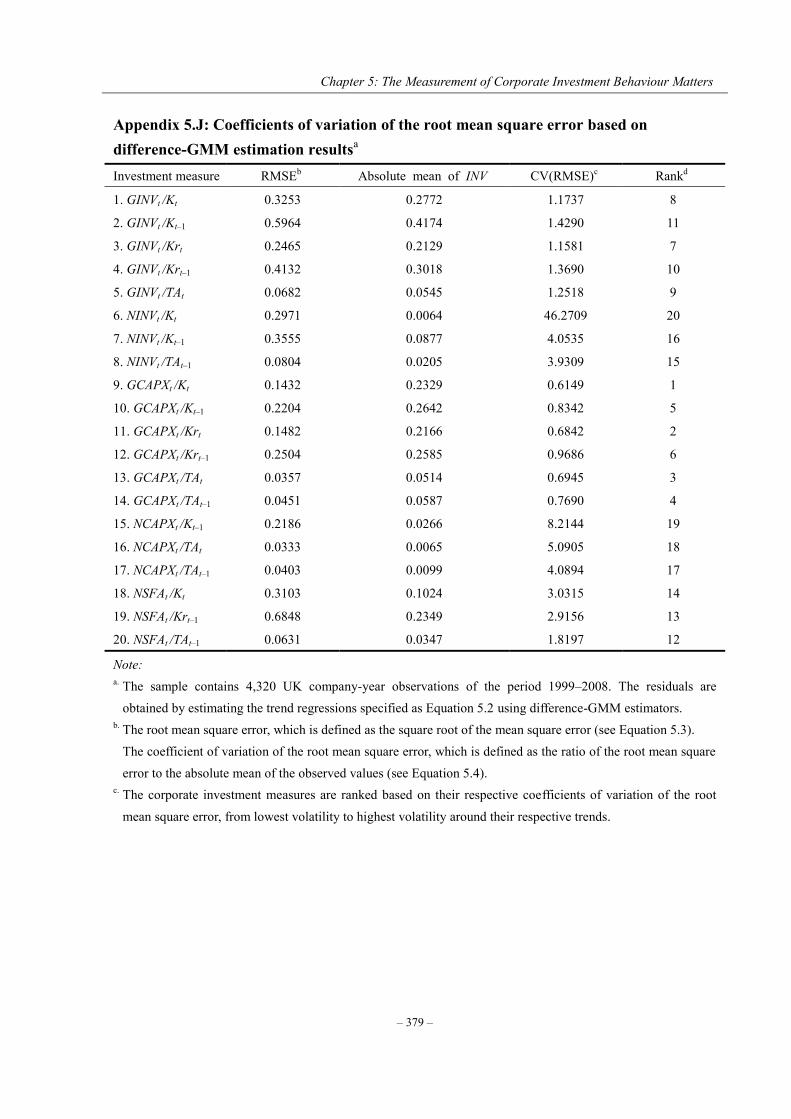
Chapter 5: The Measurement of Corporate Investment Behaviour Matters
– 379 –
Appendix 5.J: Coefficients of variation of the root mean square error based on difference-GMM estimation resultsa Investment measure RMSEb Absolute mean of INV CV(RMSE)c Rankd
1. GINVt /Kt 0.3253 0.2772 1.1737 8
2. GINVt /Kt–1 0.5964 0.4174 1.4290 11
3. GINVt /Krt 0.2465 0.2129 1.1581 7
4. GINVt /Krt–1 0.4132 0.3018 1.3690 10
5. GINVt /TAt 0.0682 0.0545 1.2518 9
6. NINVt /Kt 0.2971 0.0064 46.2709 20
7. NINVt /Kt–1 0.3555 0.0877 4.0535 16
8. NINVt /TAt–1 0.0804 0.0205 3.9309 15
9. GCAPXt /Kt 0.1432 0.2329 0.6149 1
10. GCAPXt /Kt–1 0.2204 0.2642 0.8342 5
11. GCAPXt /Krt 0.1482 0.2166 0.6842 2
12. GCAPXt /Krt–1 0.2504 0.2585 0.9686 6
13. GCAPXt /TAt 0.0357 0.0514 0.6945 3
14. GCAPXt /TAt–1 0.0451 0.0587 0.7690 4
15. NCAPXt /Kt–1 0.2186 0.0266 8.2144 19
16. NCAPXt /TAt 0.0333 0.0065 5.0905 18
17. NCAPXt /TAt–1 0.0403 0.0099 4.0894 17
18. NSFAt /Kt 0.3103 0.1024 3.0315 14
19. NSFAt /Krt–1 0.6848 0.2349 2.9156 13
20. NSFAt /TAt–1 0.0631 0.0347 1.8197 12
Note: a. The sample contains 4,320 UK company-year observations of the period 1999–2008. The residuals are
obtained by estimating the trend regressions specified as Equation 5.2 using difference-GMM estimators. b. The root mean square error, which is defined as the square root of the mean square error (see Equation 5.3).
The coefficient of variation of the root mean square error, which is defined as the ratio of the root mean square error to the absolute mean of the observed values (see Equation 5.4).
c. The corporate investment measures are ranked based on their respective coefficients of variation of the root
mean square error, from lowest volatility to highest volatility around their respective trends.
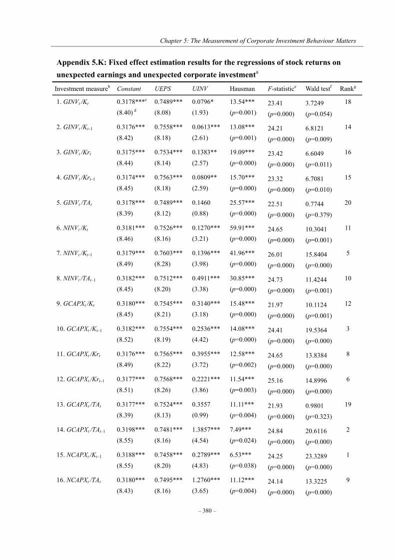
Chapter 5: The Measurement of Corporate Investment Behaviour Matters
– 380 –
Appendix 5.K: Fixed effect estimation results for the regressions of stock returns on unexpected earnings and unexpected corporate investmenta
Investment measureb Constant UEPS UINV Hausman F-statistice Wald testf Rankg
1. GINVt /Kt 0.3178***c (8.40) d
0.7489*** (8.08)
0.0796* (1.93)
13.54*** (p=0.001)
23.41 (p=0.000)
3.7249 (p=0.054)
18
2. GINVt /Kt–1 0.3176*** (8.42)
0.7558*** (8.18)
0.0613*** (2.61)
13.08*** (p=0.001)
24.21 (p=0.000)
6.8121 (p=0.009)
14
3. GINVt /Krt 0.3175*** (8.44)
0.7534*** (8.14)
0.1383** (2.57)
19.09*** (p=0.000)
23.42 (p=0.000)
6.6049 (p=0.011)
16
4. GINVt /Krt–1 0.3174*** (8.45)
0.7563*** (8.18)
0.0809** (2.59)
15.70*** (p=0.000)
23.32 (p=0.000)
6.7081 (p=0.010)
15
5. GINVt /TAt 0.3178*** (8.39)
0.7489*** (8.12)
0.1460 (0.88)
25.57*** (p=0.000)
22.51 (p=0.000)
0.7744 (p=0.379)
20
6. NINVt /Kt 0.3181*** (8.46)
0.7526*** (8.16)
0.1270*** (3.21)
59.91*** (p=0.000)
24.65 (p=0.000)
10.3041 (p=0.001)
11
7. NINVt /Kt–1 0.3179*** (8.49)
0.7603*** (8.28)
0.1396*** (3.98)
41.96*** (p=0.000)
26.01 (p=0.000)
15.8404 (p=0.000)
5
8. NINVt /TAt–1 0.3182*** (8.45)
0.7512*** (8.20)
0.4911*** (3.38)
30.85*** (p=0.000)
24.73 (p=0.000)
11.4244 (p=0.001)
10
9. GCAPXt /Kt 0.3180*** (8.45)
0.7545*** (8.21)
0.3140*** (3.18)
15.48*** (p=0.000)
21.97 (p=0.000)
10.1124 (p=0.001)
12
10. GCAPXt /Kt–1 0.3182*** (8.52)
0.7554*** (8.19)
0.2536*** (4.42)
14.08*** (p=0.000)
24.41 (p=0.000)
19.5364 (p=0.000)
3
11. GCAPXt /Krt 0.3176*** (8.49)
0.7565*** (8.22)
0.3955*** (3.72)
12.58*** (p=0.002)
24.65 (p=0.000)
13.8384 (p=0.000)
8
12. GCAPXt /Krt–1 0.3177*** (8.51)
0.7568*** (8.26)
0.2221*** (3.86)
11.54*** (p=0.003)
25.16 (p=0.000)
14.8996 (p=0.000)
6
13. GCAPXt /TAt 0.3177*** (8.39)
0.7524*** (8.13)
0.3557 (0.99)
11.11*** (p=0.004)
21.93 (p=0.000)
0.9801 (p=0.323)
19
14. GCAPXt /TAt–1 0.3198*** (8.55)
0.7481*** (8.16)
1.3857*** (4.54)
7.49*** (p=0.024)
24.84 (p=0.000)
20.6116 (p=0.000)
2
15. NCAPXt /Kt–1 0.3188*** (8.55)
0.7458*** (8.20)
0.2789*** (4.83)
6.53*** (p=0.038)
24.25 (p=0.000)
23.3289 (p=0.000)
1
16. NCAPXt /TAt 0.3180*** (8.43)
0.7495*** (8.16)
1.2760*** (3.65)
11.12*** (p=0.004)
24.14 (p=0.000)
13.3225 (p=0.000)
9

Chapter 5: The Measurement of Corporate Investment Behaviour Matters
– 381 –
Investment measureb Constant UEPS UINV Hausman F-statistice Wald testf Rankg
17. NCAPXt /TAt–1 0.3187*** (8.48)
0.7489*** (8.18)
1.2075*** (3.86)
10.71*** (p=0.005)
23.92 (p=0.000)
14.8996 (p=0.000)
7
18. NSFAt /Kt 0.3179*** (8.43)
0.7662*** (8.20)
0.0940*** (2.74)
19.95*** (p=0.000)
21.82 (p=0.000)
7.5076 (p=0.006)
13
19. NSFAt /Krt–1 0.3178*** (8.45)
0.7511*** (8.17)
0.0393** (2.39)
14.87*** (p=0.000)
22.11 (p=0.000)
5.7121 (p=0.017)
17
20. NSFAt /TAt–1 0.3187*** (8.49)
0.7710*** (8.33)
0.7384*** (4.11)
11.24*** (p=0.004)
23.03 (p=0.000)
16.8921 (p=0.000)
4
Note: a. The sample contains 4,320 UK company-year observations of the period 1999–2008. The model specified in
Equation 5.5 is estimated by fixed effect estimators using Stata 11. b. Unexpected change in corporate investment measures are used as an explanatory variable in their respective
regressions. The regression is specified as
itititit eUINVUEPSMAR 210 We also control for time effects by adding a set of year dummy variables.
c. * significant at the 10% level; ** significant at the 5% level; and *** significant at the 1% level. d. t-statistics are reported in parentheses. e. The Hausman test is implemented to test for whether the individual effect is correlated with regressors. The test
compares the coefficients obtained from both fixed effect and random effect estimators. Under the null hypothesis that individual effects are random, the fixed effect and random effect estimates should be similar because both are consistent. Under the alternative hypothesis, the fixed effect and random effect estimators diverge due to the inconsistence of random effects estimators, and thus the fixed effect estimator should be used. The test statistic asymptotically follows the Chi-squared distribution.
f. We perform Wald test to test the null hypothesis that the coefficient on UINV is equal to zero. The test reports results using the F-statistic. The associated p-value is reported in parenthesis.
g. The corporate investment measures are ranked based on their respective Wald test results, from the most
informative to the lowest informative.
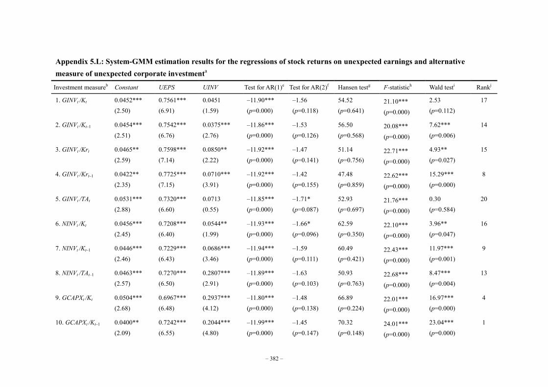
– 382 –
Appendix 5.L: System-GMM estimation results for the regressions of stock returns on unexpected earnings and alternative measure of unexpected corporate investmenta
Investment measureb Constant UEPS UINV Test for AR(1)e Test for AR(2)f Hansen testg F-statistich Wald testi Rankj
1. GINVt /Kt 0.0452*** (2.50)
0.7561*** (6.91)
0.0451 (1.59)
–11.90*** (p=0.000)
–1.56 (p=0.118)
54.52 (p=0.641)
21.10*** (p=0.000)
2.53 (p=0.112)
17
2. GINVt /Kt–1 0.0454*** (2.51)
0.7542*** (6.76)
0.0375*** (2.76)
–11.86*** (p=0.000)
–1.53 (p=0.126)
56.50 (p=0.568)
20.08*** (p=0.000)
7.62*** (p=0.006)
14
3. GINVt /Krt 0.0465** (2.59)
0.7598*** (7.14)
0.0850** (2.22)
–11.92*** (p=0.000)
–1.47 (p=0.141)
51.14 (p=0.756)
22.71*** (p=0.000)
4.93** (p=0.027)
15
4. GINVt /Krt–1 0.0422** (2.35)
0.7725*** (7.15)
0.0710*** (3.91)
–11.92*** (p=0.000)
–1.42 (p=0.155)
47.48 (p=0.859)
22.62*** (p=0.000)
15.29*** (p=0.000)
8
5. GINVt /TAt 0.0531*** (2.88)
0.7320*** (6.60)
0.0713 (0.55)
–11.85*** (p=0.000)
–1.71* (p=0.087)
52.93 (p=0.697)
21.76*** (p=0.000)
0.30 (p=0.584)
20
6. NINVt /Kt 0.0456*** (2.45)
0.7208*** (6.40)
0.0544** (1.99)
–11.93*** (p=0.000)
–1.66* (p=0.096)
62.59 (p=0.350)
22.10*** (p=0.000)
3.96** (p=0.047)
16
7. NINVt /Kt–1 0.0446*** (2.46)
0.7229*** (6.43)
0.0686*** (3.46)
–11.94*** (p=0.000)
–1.59 (p=0.111)
60.49 (p=0.421)
22.43*** (p=0.000)
11.97*** (p=0.001)
9
8. NINVt /TAt–1 0.0463*** (2.57)
0.7270*** (6.50)
0.2807*** (2.91)
–11.89*** (p=0.000)
–1.63 (p=0.103)
50.93 (p=0.763)
22.68*** (p=0.000)
8.47*** (p=0.004)
13
9. GCAPXt /Kt 0.0504*** (2.68)
0.6967*** (6.48)
0.2937*** (4.12)
–11.80*** (p=0.000)
–1.48 (p=0.138)
66.89 (p=0.224)
22.01*** (p=0.000)
16.97*** (p=0.000)
4
10. GCAPXt /Kt–1 0.0400** (2.09)
0.7242*** (6.55)
0.2044*** (4.80)
–11.99*** (p=0.000)
–1.45 (p=0.147)
70.32 (p=0.148)
24.01*** (p=0.000)
23.04*** (p=0.000)
1

– 383 –
Investment measureb Constant UEPS UINV Test for AR(1)e Test for AR(2)f Hansen testg F-statistich Wald testi Rankj
11. GCAPXt /Krt 0.0363* (1.85)
0.7002*** (6.59)
0.3186*** (4.14)
–11.83*** (p=0.000)
–1.56 (p=0.118)
72.22 (p=0.115)
23.78*** (p=0.000)
17.14*** (p=0.000)
3
12. GCAPXt /Krt–1 0.0481** (2.46)
0.7003*** (6.80)
0.1648*** (4.01)
–11.89*** (p=0.000)
–1.52 (p=0.128)
70.26 (p=0.149)
21.48*** (p=0.000)
16.08*** (p=0.000)
5
13. GCAPXt /TAt 0.0547*** (3.09)
0.7411*** (6.93)
0.8594*** (2.93)
–11.88*** (p=0.000)
–1.56 (p=0.118)
54.70 (p=0.634)
21.60*** (p=0.000)
8.58*** (p=0.004)
12
14. GCAPXt /TAt–1 0.0444** (2.41)
0.7162*** (6.82)
1.1106*** (4.57)
–11.97*** (p=0.000)
–1.31 (p=0.190)
64.51 (p=0.290)
22.82*** (p=0.000)
20.88*** (p=0.000)
2
15. NCAPXt /Kt–1 0.0327*** (1.75)
0.7098*** (6.64)
0.1604*** (4.01)
–11.80*** (p=0.000)
–1.60 (p=0.109)
66.32 (p=0.239)
23.35*** (p=0.000)
16.08*** (p=0.000)
6
16. NCAPXt /TAt 0.0365** (2.05)
0.7251*** (6.90)
0.9310*** (3.23)
–11.93*** (p=0.000)
–1.55 (p=0.121)
62.83 (p=0.342)
21.76*** (p=0.000)
10.43*** (p=0.001)
11
17. NCAPXt /TAt–1 0.0393*** (2.20)
0.7203*** (6.95)
0.9200*** (3.95)
–11.93*** (p=0.000)
–1.47 (p=0.141)
60.06 (p=0.437)
22.26*** (p=0.000)
15.60*** (p=0.000)
7
18. NSFAt /Kt 0.0336*** (1.87)
0.7375*** (7.12)
0.0331 (1.16)
–11.85*** (p=0.000)
–1.62 (p=0.105)
57.35 (p=0.536)
21.79*** (p=0.000)
1.35 (p=0.246)
19
19. NSFAt /Krt–1 0.0498*** (2.62)
0.6741*** (6.28)
0.0167 (1.53)
–11.83*** (p=0.000)
–1.74* (p=0.081)
59.45 (p=0.459)
18.35*** (p=0.000)
2.34 (p=0.127)
18
20. NSFAt /TAt–1 0.0288*** (1.53)
0.7216*** (6.67)
0.5006*** (3.44)
–11.90*** (p=0.000)
–1.43 (p=0.152)
68.60 (p=0.1839)
21.37*** (p=0.000)
11.83*** (p=0.001)
10
Note: a. The sample contains 4,320 UK company-year observations for the period 1999–2008. The model specified in Equation 5.5 is estimated by two-step system-GMM
estimators using Stata 11.

– 384 –
b. The alternative measures of unexpected change in corporate investment are used as an explanatory variable in their respective regressions. The model is specified as
itititit eUINVUEPSMAR 210 We also control for time effects by adding a set of year dummy variables. The instruments used for the regression include Constant, Year dummies, UEPSt-1…, t-3, UINVt-1…, t-3, ∆Year dummies, ∆UEPSt and ∆UINVt.
c. * significant at the 10% level; ** significant at the 5% level; and *** significant at the 1% level. d. t-statistics are reported in parentheses. e. The Arellona-Bond test tests for serial correlation in the first-differenced errors in order to purge the unobserved and perfectly autocorrelated individual effects.
Autocorrelation at order 1 is expected in first differences, because 1 ititit should correlate with 211 ititit , since they share the 1it term. f. To check for AR(1) in levels, look for AR(2) in differences, in the idea that this will detect the relationship between the 1it in it and the 2it in 2 it .
Autocorrelation indicates that lags of the dependent variable (and any other variables used as instruments that are not strictly exogenous), are in fact endogenous, thus bad instruments. Therefore, rejecting the null hypothesis of no serial correlation in the first-differenced errors at an order greater than one implies model misspecification.
g. The Hansen overidentifying restrictions test tests for whether the instruments, as a group, appear exogenous. Under two-step robust GMM estimation, the Sargan statistic is not robust to heteroscedasticity or autocorrelation, but the Hensen J-statistic, which is the minimised value of the two-step GMM criterion function, is robust. The joint null hypothesis is that the instruments are valid instruments, i.e. uncorrelated with the error term, and that the excluded instruments are correctly excluded from the estimated equation. A statistically significant test statistic always indicates that the instruments may not be valid. However, the J-test has its own problem: it can be greatly weakened by instrument proliferation.
h. F-statistic for the regression which tests the null hypothesis that all of the coefficients except the intercept coefficient are jointly zero. i. We perform Wald test to test the null hypothesis that the coefficient on UINV is equal to zero. The test reports results using the F-statistic. The associated p-value is
reported in parenthesis. j. The corporate investment measures are ranked based on their respective Wald test results from the highest informative to lowest informative.
Chapter 6: Conclusion
– 385 –
CHAPTER 6
CONCLUSION
6.1 Summary
This thesis empirically investigates the interdependence of corporate investment, financing
and payout decisions in the presence of financial constraints, with reference to a large panel of
UK-listed companies observed within the period from 1999 to 2008, in an attempt to improve
our current knowledge of the simultaneity of the execution of corporate decisions. It also
represents one of the first studies to explicitly and systematically examine the influence of
uncertainty and managerial confidence on the set of jointly determined corporate decisions
within a simultaneous equations system. The simultaneous equations framework explicitly
allows uncertainty and managerial confidence to not only affect each of the corporate
decisions directly on their own, but also indirectly through their effect on other decisions.
Such analyses reveal new insights into the role played by companies’ fundamental uncertainty
and by managers’ psychological bias in determining aspects of corporate behaviour. In
addition, this thesis offers, for the first time, a comparison and evaluation of the alternative
measures of corporate investment that are currently utilised in applied corporate finance
studies. It, therefore, sheds some light and provides some guidance for measuring corporate
investment behaviour.
This chapter concludes the thesis by briefly recapping the research questions,

Chapter 6: Conclusion
– 386 –
summarising the key findings, highlighting the main contributions, discussing the broad
implications, acknowledging the limitations, as well as offering some promising ideas for
further research.
6.2 Key empirical findings and conclusions
6.2.1 Simultaneous determination of corporate decisions
The comprehensive review of existing literature shows that, although much effort has been
devoted to investigating this key set of corporate decisions, corporate investment, financing
and payout decisions have typically been treated separately and examined in isolation rather
than altogether, and hence there has been little analysis of the simultaneity among them. Prior
research, however, has provided both reasons and evidence that corporate investment,
financing and payout decisions are likely to be interdependent upon one another and jointly
determined by management. Several mechanisms through which the set of corporate decisions
may be related to one another have been explored, such as the institutional approach,
flow-of-funds approach, tax approach, agency approach, information approach, etc. An
important implication is that corporate investment, financing and payout decisions are
potentially linked in several important ways, thus should be better analysed within a
simultaneous model framework. However, previous studies on the simultaneous
determination of corporate decisions are not sufficiently comprehensive, in the sense that they
neither provide enough insight into the theoretical mechanism through which the set of
Chapter 6: Conclusion
– 387 –
corporate decisions are likely to be simultaneously determined, nor offer solid empirical
evidence which can verify the potential interactions suggested by the theoretical arguments.
Nonetheless, previous studies provide us with guidance in modelling corporate behaviours to
avoid the danger of drawing spurious conclusions.
To fill this gap in the existing literature, Chapter 3 investigates the interactions among
corporate investment, financing and payout decisions in the presence of financial constraints,
with reference to the UK-listed companies. The three main aspects of corporate behaviour are
modelled within a simultaneous equations system where they are treated as endogenous. On
the whole, our results suggest that corporate investment, financing and payout decisions are
indeed inextricably linked and jointly determined by UK-listed companies, as implied by the
information asymmetry-based flow-of-funds framework for corporate behaviour. It is found
that capital investment and dividend payout, as competing uses of limited funds, are
negatively interrelated, and both are positively interrelated to internally generated cash flow
and the net amount of new debt issued. These results suggest that UK-listed companies are
likely to be financially constrained not only by the availability of internal funds but also by
the access to external finance, and therefore managers have to consider their financing and
payout choices alongside with their investment decisions.
Furthermore, we divide the entire sample into financially more constrained and less
constrained subsamples and analyse them separately, in an attempt to gain deeper insights into
the mechanisms through which the set of corporate decisions interrelated with one another. By
Chapter 6: Conclusion
– 388 –
comparing the magnitude and significance of coefficients on the endogenous variables across
the two subsamples results, we find that simultaneity among the three corporate decisions is
more pronounced for financially more constrained companies, whist that for less constrained
companies is relatively weak. Our empirical results indicate that the substantial economic
interactions among the set of corporate decisions observed from UK-listed companies are
likely to be attributable to financial constraints.
6.2.2 Corporate decisions under uncertainty
The review of literature also shows that uncertainty associated with a company’s future
prospects seems to be a critical factor in determining corporate investment behaviour, as
highlighted by the real options theory of investment. A broad consensus in existing empirical
research is that the effect of uncertainty on investment is negative, although a number of
studies also suggest that relationship between uncertainty and investment might be positive or
non-linear. However, prior research has largely ignored the importance of uncertainty in
financial decisions as well as the potential influence of uncertainty on investment through its
effects on financing and payout choices. Given the fact that all corporate decisions are
determined on the basis of uncertain information, the omission of relevant information in
examining the effect of uncertainty on corporate investment is likely to generate misleading
results and lead to inappropriate inferences. Therefore, it is more plausible to model corporate,
financing and payout decisions simultaneously, and to investigate the effect of uncertainty on
aspects of corporate behaviour within the simultaneous equations system.
Chapter 6: Conclusion
– 389 –
In order to comprehensively investigate corporate behaviour under uncertainty,
Chapter 3 offers the first systematic attempt to uncover the influences of uncertainty on
aspects of corporate behaviour. By examining the effects of uncertainty on corporate decisions
within the simultaneous equations system, this thesis offers new insight into the role
uncertainty plays, not only as one of the key determinants of real investment decisions, but
also as a key factor affecting corporate financial decisions which has been overlooked by the
existing literature. We find that the effect of uncertainty on corporate investment is positive
and significant, while that of uncertainty on dividend payouts is negative and also significant,
suggesting that uncertainty stimulates investment in capital stock, not only on its own but also
through its effect on dividend payout policy. Accordingly, companies facing greater
uncertainty appear to invest more, and fund the increased investment by resorting to internal
finance by cutting dividends rather than resorting to external finance by issuing new debts.
In addition, we find that the effect of uncertainty is more significant for financially
less constrained companies but insignificant for more constrained ones, suggesting that less
constrained companies respond to uncertainty more aggressively than more constrained ones.
Therefore, our results offer new insights that financial constraints not only intensify the
simultaneity among corporate investment, financing and payout decisions, but also reduce
managerial flexibility in adjusting those corporate decisions to respond to uncertainty.
6.2.3 Corporate decisions and the state of confidence
Recently, an emerging body of literature on behavioural corporate finance uncover that
Chapter 6: Conclusion
– 390 –
managers’ psychological bias may have substantial impact on corporate decisions. In
particular, managers’ upwards bias towards future company performance may generate
overinvestment, underinvestment and pecking order financing behaviours through different
channels. Prior research in this area mainly focuses either on the influences of investor
sentiment (e.g. Polk and Sapienza, 2009), or on the impacts of managers’ personality traits on
corporate behaviour (e.g. Malmendier et al., 2011; Hackbarth, 2008; and Malmendier and
Tate, 2005). However, little research has been undertaken on the influences of the state of
managerial confidence or economic sentiment at aggregate levels on aspects of corporate
behaviour, despite it often being argued that this has some bearing on corporate
decision-making processes. Although the theoretical framework in this emerging area has not
been firmly established and the empirical evidence is still relatively rare, it is plausible to
hypothesise that the less than fully rational manager approach to behavioural corporate
finance has the potential to explain a wide range of patterns in corporate investment, financing
and payout decisions.
By relaxing the conventional assumption that managers are fully rational, Chapter 4
offers the first attempt to investigate the impacts of managerial confidence and economic
sentiment at aggregate levels on the jointly determined corporate investment, financing and
payout decisions, using data from the panel of UK-listed companies observed within the
period from 1999 to 2008. The relations between corporate decisions and the state of
sentiment and confidence are examined within a simultaneous equations system which allows

Chapter 6: Conclusion
– 391 –
for contemporaneous interdependence among the corporate decisions. The empirical results
show that the state of confidence at aggregate levels, as proxied by the UK or EU managerial
confidence indicators or economic sentiment indicators, has significantly positive effects on
companies’ real investment and debt financing decisions. The positive effects remain
statistically significant even after controlling for company idiosyncratic uncertainty and other
fundamental variables. These findings show that managerial psychological bias plays an
important role in the determination of corporate decisions, adding new evidence to the small
but growing literature on behavioural corporate finance.
In addition, the results presented in Chapter 4 also provide empirical evidence that
managers’ psychological bias and companies’ fundamental uncertainty influence corporate
decisions independently through different channels. Both managerial confidence and
fundamental uncertainty have positive real effects on corporate investment decisions.
However, managers consider different financial choices in response to the increased financing
needs caused by different factors. To finance the increased investment spending caused by
high managerial confidence and economic sentiment, companies tend to use external debt
financing rather than cutting dividends paid to their shareholders. To financing the increased
investment spending under a high level of uncertainty, companies prefer to resort to internal
finance by cutting dividends rather than resorting to external finance by issuing new debts.
Moreover, we find that companies in the services sector behave more aggressively compared
to others when their managers are confident. Specifically, they invest in capital stock more
Chapter 6: Conclusion
– 392 –
intensively, use debt financing more heavily, and cut dividends more decisively when the
sentiment is high.
6.2.4 Measurement of corporate investment behaviour
The review of corporate finance literature also shows that the use of the corporate investment
to capital stock ratio as a measure of corporate investment behaviour has been common
practice in applied studies. Although the corporate investment ratios used in the existing
literature are similarly specified and interpreted in the same way, they in fact vary both on the
numerator and the denominator. At least twenty different constructions of corporate
investment to capital stock ratio have been identified in the existing literature. However, no
attempt has been made to provide a comparison among various corporate investment
measures. One claim which has been implicitly made is that different measures of corporate
investment behaviour will always yield the same, or at least qualitatively similar, results in
empirical analyses. As a consequence, we know little about how differently these corporate
investment measures perform in empirical analyses, and the extent to which the choice of
corporate investment measures may influence the conclusions drawn from empirical analyses.
Chapter 5, therefore, aims to fill this important gap in the literature by discriminating
conceptually and evaluating empirical twenty different measures of corporate investment that
are currently used in applied studies. The various corporate investment measures are first
discriminated from an accounting perspective. Given the fact that different accounting
Chapter 6: Conclusion
– 393 –
principles as well as different elements are involved in the construction of the alternative
corporate investment measures, they are likely to carry different sets of information about a
company’s investing activities. Information about a company’s future prospects contained in
one corporate investment measure may not necessarily present in others, and vice versa. Due
to a lack of understanding of the financial information provided by the relevant accounting
items, corporate investment measures are potentially misused in empirical analyses. The
conflicting conclusions drawn from the empirical literature on corporate investment, therefore,
may also be attributable to the differences in measuring companies’ investment behaviour.
With a balanced panel of UK-listed companies over the period 1999–2008, we
empirically demonstrate that the alternative corporate investment measures are not uniformly
positively correlated with one another. Significantly negative correlations are also observed
among the alternatives, which appear surprising, since they are supposed to measure the
investment behaviour of the same batch of companies over the same period of time. Therefore,
there is no reason to expect the different measures of corporate investment ratio to yield
equivalent results in empirical analyses. Accordingly, we posit that the conclusions drawn
from empirical analyses are likely to be sensitive to the choice of corporate investment
measures. This prediction is empirically verified by repeatedly estimating a simple Tobin’s Q
model of investment, which indicates that the measurement of corporate investment behaviour
does indeed matter in empirical analyses.
To assess the empirical performance of the alternative corporate investment measures,
Chapter 6: Conclusion
– 394 –
we carry out both trend analysis and information content analysis. The empirical results
suggest that gross investment measures are systematically less noisy compared to the net
investment measures, while cash based corporate investment measures are systematically
more informative than their accrual based counterparts. Accordingly, we conclude that cash
based gross corporate investment to capital stock ratios are the best performing measures of
corporate investments behaviour among the alternatives, as they contain relatively less noise
and greater value relevant information. Researchers in the area of corporate finance, therefore,
are suggested to utilise cash based gross corporate investment measures for their future
empirical analyses if they have to make mutually exclusive choices among the alternatives
without any particular preference.
6.3 Main contributions to the existing literature
This thesis aims to fill the critical lacunae identified in the existing corporate finance literature,
by investigating corporate investment, financing and payout decisions simultaneously, with
reference to a large panel of UK-listed companies. Based on an implicit flow-of-funds
framework for corporate behaviour, we develop a simultaneous equations system that
explicitly accounts for the interdependence among the three corporate decisions, with each of
the decisions being treated as endogenous. Furthermore, the simultaneous equations system is
also used as a platform for undertaking empirical investigations into the influences of
fundamental uncertainty and sentimental bias on the set of jointly determined corporate
decisions. Conducting such a study makes a number of important contributions to the existing
Chapter 6: Conclusion
– 395 –
literature, which we believe, would enhance our understanding of the complex corporate
decision-making process in the real world.
Specifically, the main contributions of this thesis are fivefold. First, unlike previous
studies that focus only on one aspect of corporate behaviour, we treat corporate investment,
financing and payout decisions endogenously, and model them simultaneously within a
system as implied by an implicit flow-of-funds framework for corporate behaviour. By
utilising recent econometric methods for simultaneity analysis, this research overcomes the
shortcomings of single equation techniques currently adopted in the existing literature, and
provides new insight into the interdependences among the corporate decisions in practice. The
interactions among the corporate decisions are empirically verified in Chapter 3 and further
confirmed in Chapter 4 based on the evidence obtained from UK-listed companies,
contributing to the current knowledge of the complex interdependence of corporate behaviour
under financial constraints.
Second, we explicitly explore the possible channel through which the set of corporate
decisions are interdependent upon one another, in order for us to fully facilitate the corporate
decision-making process. By splitting the entire sample into two subsamples with financially
more constrained and less constrained companies respectively, we find that the simultaneity
among the three corporate decisions is more pronounced for financially more constrained
companies, whist that for financially less constrained companies is relatively weak. This
indicates that the substantial economic interactions among the set of corporate decisions

Chapter 6: Conclusion
– 396 –
observed from UK-listed companies are likely to be caused by financial constraints. The
findings offered in Chapter 3 are helpful in explaining the joint determination of corporate
decisions in practice.
Third, this thesis offers the first systematic attempt to uncover the influences of
uncertainty on aspects of corporate behaviour. By examining the effects of uncertainty on
corporate decisions within the simultaneous equations system, this thesis offers new insight
into the role uncertainty plays, not only as one of the key determinants of real investment
decisions, but also as a key factor affecting corporate financial decisions which has been
overlooked by the existing literature. In addition, we find that financially less constrained
companies tend to behave differently under uncertainty from financially more constrained
ones. This thesis, therefore, extends the existing literature on corporate behaviour under
uncertain circumstances. This is again achieved in Chapter 3.
Fourth, this thesis represents one of the first studies to explicitly and systematically
investigate the influences of the state of confidence at aggregate levels on the set of jointly
determined corporate decisions. By relaxing the conventional assumption of broad rationality,
the study highlights the importance of managers’ psychological bias, as proxied by managerial
confidence and economic sentiment indicators, in the determination of the corporate decisions.
The findings with regard to the influence of the state of confidence on aspects of corporate
behaviour persist even after controlling for company-level uncertainty and other company
fundamental characteristics, indicating that the state of confidence and the level of
Chapter 6: Conclusion
– 397 –
fundamental uncertainty affect corporate behaviour independently through different channels.
The research work presented in Chapter 4 adds empirical evidence to the small but growing
strand of literature on behavioural corporate finance.
Finally, the comprehensive review of literature shows that the use of corporate
investment to capital stock ratio as a measure of corporate investment behaviour in empirical
analyses has become a common practice. However, to the best of our knowledge, there has
been no literature that provides a comparison among the various versions of corporate
investment ratio which seem at first sight very similarly constructed. An attempt is made in
this thesis to conceptually discriminate and statistically compare twenty alternative measures
of corporate investment which have been identified in the existing literature. The evaluation
results presented in Chapter 5 not only provide some guidance for measuring corporate
investment behaviour in future empirical analyses, but also to some extent explain the
inconsistent evidence and conflicting conclusions in the existing empirical literature on
corporate investment.
6.4 Practical implications of the findings
The findings and conclusions presented in this thesis not only contribute to the existing
academic literature, but also have broader practical implications, especially for corporate
managers, public policy makers and investors.
Chapter 6: Conclusion
– 398 –
6.4.1 Implications for corporate managers
Since our investigation focuses particularly on the simultaneity as well as determinants of
corporate investment, financing and payout decisions of UK-listed companies, we first
consider the practical implications for corporate managers.
First, the interactions among corporate investment, financing and payout decisions
evidenced in this study have distinct implications for companies and their managements. In
making key corporate decisions, managers must be aware of the inherent interactions which
exist among them, in order to avoid undesirable side effects which may stem from a given
decision. Thus, managers should consider the key corporate decisions simultaneously, or if the
decisions are taken piece meal due consideration must be paid to the influence of the other
factors. Particularly, in the presence of financial constraints, companies have to consider their
fund-raising choices alongside their fund-spending decisions, in an attempt to prevent losses
from underinvestment and at the same time to keep their overall cost of capital as low as
possible, such that shareholders’ wealth can be maximized.
Second, the empirical evidence on the relationship between investment and
uncertainty uncovered in this study also has profound implications for corporate decision
makers. Our results indicate that, in a competitive business environment, uncertainty
associated with future prospects tends to increase not only the value of real option but also the
advantage of pre-emption. In such a multi-player context, selectivity, value and timing of a
company’s investments are likely to be influenced by the similar investment decisions made

Chapter 6: Conclusion
– 399 –
by its peers. Managers therefore need to consider the strategic interactions among the peers in
making corporate investment decisions. If there a strong and persistent advantage to be the
first to invest, companies might be better off by investing earlier to pre-empt their rivals in
spite of the uncertain outcomes.
Third, it is found that managers are likely to be overconfident in making corporate
decisions, and their upward psychological bias towards their companies’ future performance
may result in distortions in corporate decisions. Although the less than fully rational
managerial behaviour is fundamentally different from the rational moral hazard behaviour in
the sense that managers believe that they are maximising their company’s value, managers’
upward psychological bias are likely to result in unintended overinvestment problems and
simultaneously make their companies over indebted, which may damage shareholders’ wealth.
These unintended distortions in corporate behaviour caused by managerial overconfidence
cannot even be mitigated by using conventional incentives such as stock- or option-based
compensation, as indicated in earlier work by Malmendier et al. (2011). Therefore, in order to
better serve shareholders’ interests, innovative contracting practices and organizational
designs are needed to constrain managers’ upward psychological bias.
6.4.2 Implications for public policy makers
Although this study focuses primarily on aspects of corporate behaviour, the empirical
findings and conclusions drawn from this thesis may also have some implications for public
policy makers.
Chapter 6: Conclusion
– 400 –
First, our empirical results suggest that the corporate investments of UK-listed
companies are likely to be financially constrained not only by the insufficient availability of
internal funds but also by the limited access to external funds. It is evident that financially less
constrained companies are able to invest more efficiently by putting more weight on their real
considerations in making corporate investment decisions, whereas the investments of
financially more constrained companies are highly sensitive to their financial choices.
Previous studies, such as Bond et al. (2003), indicate that, compared with the continental
European financial system, the market-oriented financial system in the UK perform less well
in channelling investment funds to companies with profitable investment opportunities
because of the information asymmetry results from the arm’s-length relation between
companies and suppliers of finance. Therefore, an important implication for public policy
makers is that, by mitigating the degree of information asymmetry, which seems to be severe
in the UK financial system, a more accommodative environment for business activities, in
terms of corporate investment and financing, can be created.
Second, it is found that managerial confidence and economic sentiment play a key role
in the formation of companies’ expectations of future returns and risks, and thus in the
determination of corporate decisions. High levels of confidence and sentiment encourage
companies to take on more debt, which in turn enables them to invest more in capital assets.
Therefore, the extent to which a policy stimulus contributes to an improvement in managerial
confidence and economic sentiment is likely to be highly important. This implication is
Chapter 6: Conclusion
– 401 –
particularly relevant for the public policy makers who are trying to stimulate corporate
investment spending amid the on-going global financial crisis. In addition, certain level of
uncertainty may also encourage companies to investment earlier in a competitive market
environment, because the threat of being pre-empted may offset the value of the real option.
Third, our simultaneous analyses show that corporate investment spending and
dividend payout are competing uses of limited funds, and the negative relationship between
the two variables may also have some implications for policy makers. It has long been argued
that, in comparison to the classical system, the imputation tax system in the UK encourages
companies to pay dividends rather than retain their profits (see, for example, Adedeje, 1998).
Such a tax system therefore may exert a negative influence on corporate investment spending
in the long run. Given this negative interaction between corporate investment and dividend
payout decisions, government might be able to encourage corporate sector’s investment
spending by adjusting its tax policy on dividends.
6.4.3 Implications for investors
In addition to the implications for corporate managers and public policy makers, the empirical
evidence presented in this thesis also has implications for investors in general.
The simultaneous analysis clearly shows that a company’s dividend decision is neither
totally residual nor completely independent, but is taken with reference to its investment and
financing decisions. In practice, investors seem to have strong preferences for high dividend
payout ratios as they consider it as a sign that directors are alive to their shareholders.

Chapter 6: Conclusion
– 402 –
However, investors may have not thought through the interactions that exist between dividend
payout and corporate investment, and between dividend payout and debt financing. If fact, the
size of dividend paid to shareholders directly affect both capital investment and debt financing
decisions made by a company. If investors constantly put a high premium on dividend payers,
companies might be forced either to forego relatively low net present value investment
projects or to raise more external funds through a catering channel, resulting in either
underinvestment losses or flotation costs. Therefore, an important implication for investors is
that high levels of dividend payouts are not always in the best interest of shareholders.
Shareholders should consider dividends paid by a company in the contest of the company’s
investment opportunities and financing abilities.
6.5 Limitations of the research
It is worth noting that there are several limitations of the research reported in this thesis. First,
the research relies mainly on the empirical research methodology, as illustrated by Figure 1.1,
to test theoretical predictions. The findings and conclusions of this thesis are largely drawn
from the accumulation of evidence collected from the dataset. Hence, the first main limitation
of this thesis is that the validity of the conclusions may, to some extent, be sensitive to the
selection of the sample, the measurement of variables, the specification of models, the choice
of estimation techniques and the interpretation of results. Given the fact that a large amount of
financial and accounting information is used to produce the empirical evidence, the results
presented in this thesis may also be subject to the managerial manipulation of the reported
Chapter 6: Conclusion
– 403 –
accounting data.
Second, this thesis does not attempt to develop theoretical models and proofs on
corporate finance issues. By using statistical hypothesis testing methods, we can only find
empirical evidence to support or reject the theoretical predictions implied by the existing
corporate finance theories, rather than prove them. Thus, theoretical issues in corporate
finance are not explicitly addressed in this thesis.
Third, although this thesis tries to systematically and simultaneously investigate the
key corporate decisions within a framework as a whole, some important issues relating to
corporate finance, such as corporate governance, initial public offering and seasoned equity
offering, are not addressed here, owning to the lack of availability of relevant data. In
particular, external equity financing is dropped from the flow-of-funds framework for
simplicity, and thus the importance of financing through stock issuance is overlooked.
Besides this, since the thesis is produced by combining four stand-alone research
papers, presented in Chapters 2, 3, 4 and 5, there is some limited amount of overlap among
the chapters, in particular the duplication of literature review material. However, it is also
necessary to review briefly the relevant previous studies in the empirical chapters to maintain
their stand-alone status. We, therefore, allow for a limited amount of overlap among chapters,
but the amount of overlap has been minimised where possible.
Despite the above shortcomings, this research reveals new insights into the complex
corporate decision-making processes. Some of the limitations of the research are expected to
Chapter 6: Conclusion
– 404 –
be addressed in the future research.
6.6 Promising ideas for further research
Finally, a number of promising ideas for future research can be drawn from the existing
literature reviewed and the empirical findings presented in this study. We conclude this thesis
by proposing a number of promising research ideas for the further extensions of this study.
This study investigates a key set of corporate decisions within a simultaneous
equations system, as implied by the flow-of-funds framework. However, we do not consider
external equity finance as a significant source of external finance, given the argument that it is
rarely used after initial public offerings (see, for example, Cleary et al., 2007; and
Shyam-Sunder and Myers, 1999). Following the “fairly standard assumption”, external equity
financing thus has been dropped from the system for simplicity in this study. However, some
other studies, such as Frank and Goyal (2003), claim that net equity issues on average exceed
net debt issues in the US, and that net equity issues may track financing deficit more closely
than do net debt issues. Therefore, further research may incorporate external equity financing
into the simultaneous equations system, in order to explore the interactions between the
external equity financing decision and other corporate decisions modelled in the system.
Apart from the flow-of-funds framework for corporate behaviour, a number other
approaches, such as tax approach and agency approach, may also be adopted to establish
linkages among corporate investment, financing and payout decisions. These hypothesised
mechanisms are not mutually exclusive, but they may have very different implications for the
Chapter 6: Conclusion
– 405 –
interactions among the set of corporate decisions. Further research may specify simultaneous
equations systems for the set of corporate decisions in accordance with the alternative
mechanisms, to further improve our understanding of the complex corporate decision-making
process in the real world.
Contrary to the broad consensus in the existing literature that uncertainty hampers
corporate investment because of the increased value of the real “call option” to invest under
uncertain circumstances (see, for example, Bloom et al., 2007 and Carruth et al., 2000), this
study finds a significant but positive effect of uncertainty on the corporate investment of the
UK-listed companies. This finding provides empirical support for the recent argument by
Mason and Weeds (2010) that greater uncertainty can lead companies to take the advantage of
pre-emption by investing earlier under a competitive business environment. However, the
mechanism through which uncertainty stimulates corporate investment is not explicitly
explored in this study, and thus needs to be addressed in future research. One possible solution
is to classify the sample companies into monopolies and competitive companies according to
their market structures (see, for example, Lensink and Murinde, 2006), and re-estimate the
simultaneous equations system using subsamples. If Mason and Weeds’ (2010) argument
holds, we expect the positive effect of uncertainty on investment to be more significant for a
competitive company than for a monopolistic company.
The construction of an appropriate proxy for uncertainty remains as the primary
challenge faced by studies considering the effects of uncertainty on corporate behaviour.
Chapter 6: Conclusion
– 406 –
Given the inability to underpin the specific source of uncertainty, this study derives general
measures of uncertainty from stock market-based information. It is believed that, if the market
is efficient, all of the information about a company’s asset fundamentals and growth
opportunities will be properly transmitted into its share price. Thus, our measures of
uncertainty are expected to capture the overall uncertainty associated with the changing
aspects of a company’s environment. However, Carruth et al. (2000) argue that a test of the
investment-uncertainty relationship should distinguish between the effects of industry-wide
and company-specific shocks. The main concern is that irreversibility and strategic
considerations act in opposite directions, thus the two effects may cancel each other out and
lead to an inconclusive result. Therefore, another promising research idea is to decompose a
company’s total uncertainty into its market, industry and company-specific components, and
explore the effect of uncertainty at different levels on aspects of the corporate behaviour of
UK-listed companies.
Similarly, the principal challenge of incorporating the concepts of confidence into
corporate behavioural modelling is to construct plausible measures of the hard-to-define idea
(see Malmendier and Tate, 2005). In this study, we employ managerial confidence and
economic sentiment indicators as proxies for the state of confidence at aggregate levels.
However, recent literature in behavioural corporate finance has proposed a number of creative
methods to proxy managerial confidence at company level. For example, Malmendier et al.
(2011) and Malmendier and Tate (2005) exploit the overexposure of CEOs to the idiosyncratic

Chapter 6: Conclusion
– 407 –
risk of their companies, as reflected by their personal portfolio of their companies’ options
and stockholdings, to measure managerial confidence in the US. Ben-David et al. (2007)
measure overconfidence based on CFOs’ confidence intervals of their stock market
predictions. Lin et al. (2005) construct managerial confidence measures for Taiwanese
companies based on CEOs’ forecast errors in their companies’ future earnings. Unfortunately,
such data that can be used to construct measures of managerial confidence at manager level is
not readily available in the UK market. However, it is possible for further study to construct
more direct measures of managerial confidence using survey instruments. Survey responses
from corporate decision makers are expected to be better able to capture managerial confidence or
overconfidence.
It is clear that future research into corporate investment, financing and payout
decisions is required, and much more remains to be done. With the development of theoretical
frameworks and the accumulation of empirical evidence, our knowledge about aspects of
corporate behaviour will be continually improved in the future.
References
– 408 –
REFERENCES
Abdul-Haque and Wang, S. (2008). Uncertainty and investment evidence from a panel of Chinese firms. Structural Change and Economic Dynamics, 19(3), 237–248.
Abel, A. B. (1983). Optimal investment under uncertainty. American Economic Review, 73(1),
228–233. Abel, A. B., Dixit, A. K., Eberly, J. C. and Pindyck, R. S. (1996). Options, the value of capital,
and investment. Quarterly Journal of Economics, 111(3), 753–777. Abel, A. B. and Eberly, J. C. (1999). The effects of irreversibility and uncertainty on capital
accumulation. Journal of Monetary Economics, 44(3), 339–377. Adam, T. (2009). Capital expenditures, financial constraints, and the use of options. Journal
of Financial Economics, 92(2), 238–251. Adam, T. and Goyal, V. K. (2008). The investment opportunity set and its proxy variables.
Journal of Financial Research, 31(1), 41–63. Adedeji, A. (1998). Does the pecking order hypothesis explain the dividend payout ratios of
firms in the UK? Journal of Business Finance and Accounting, 25(9–10), 1127–1155. Agca, S. and Mozumdar, A. (2008). The impact of capital imperfections on investment-cash
flow sensitivity. Journal of Banking and Finance, 32(2), 207–216. Aggarwal, R. and Zong, S. (2006). The cash flow-investment relationship: international
evidence of limited access to external finance. Journal of Multinational Financial Management, 16(1), 89–104.
Ahn, S. and Denis, D. J. (2004). Internal capital markets and investment policy: evidence
from corporate spinoffs. Journal of Financial Economics, 71(3), 489–516. Aivazian, V. A., Ge, Y. and Qui, J. (2005). The impact of leverage on firm investment:
Canadian evidence. Journal of Corporate Finance, 11(1–2), 277–291. Akerlof, G. A. (1970). The market for “lemons”: quality uncertainty and the market
mechanism. Quarterly Journal of Economics, 84(3), 488–500.

References
– 409 –
Alderson, M. J. and Betker, B. L. (2006). The specification and power of tests to detect abnormal changes in corporate investment. Journal of Corporate Finance, 12(4), 738–760.
Alderson, M. J., Betker, B. L. and Stock, D. R. (2006). Investment and financing activity
following calls of convertible bonds. Journal of Banking and Finance, 30(3), 895–914.
Alicke, M. D., Klotz, M. L., Breitenbecher, D. L., Yurak, T. J. and Vredenburg, D. S. (1995).
Personal contact, individuation, and the better-than-average effect. Journal of Personality and Social Psychology, 68(5), 804–825.
Almeida, H. and Campello, M. (2007). Financial constraints, asset tangibility, and corporate
investment. Review of Financial Studies, 20(5), 1429–1460. Alti, A. (2006). How persistent is the impact of market timing on capital structure? Journal of
Finance, 61(4), 1681–1710. Arellano, M. and Bond, S. (1991). Some test of specification for panel data: Monte Carlo
evidence and an application to employment equations. Review of Economic Studies, 58(2), 277–297.
Arellano, M. and Bover, O. (1995). Another look at the instrumental variable estimation of
error-component models. Journal of Econometrics, 68(1), 29–52. Arnold, G. C. and Hatzopoulos, P. D. (2000). The theory-practice gap in capital budgeting:
evidence from the United Kingdom. Journal of Business Finance and Accounting, 27(5–6), 603–626.
Ascioglu, A., Hegde, S. P. and McBermott, J. B. (2008). Information asymmetry and
investment-cash flow sensitivity. Journal of Banking and Finance, 32(6), 1036–1048. Baker, H. K., Powell, G. E. and Veit, E. T. (2002). Revisiting managerial perspectives on
dividend policy. Journal of Economics and Finance, 26(3), 267–283. Baker, M., Ruback, R. and Wurgler, J. (2006). Behavioral corporate finance: a survey. In
Eckbo, E. (ed.), Handbook of Corporate Finance: Empirical Corporate Finance (Amsterdam: North Holland).
Baker, M. and Wurgler, J. (2002). Market timing and capital structure. Journal of Finance,
57(1), 1–32.

References
– 410 –
Baker, M. and Wurgler, J. (2004). A catering theory of dividends. Journal of Finance, 59(3), 1125–1165.
Bakke, T. and Whited, T. M. (2010). Which firms follow the market? An analysis of corporate
investment decisions. Review of Financial Studies, 23(5), 1941–1980. Bali, R. (2003). An empirical analysis of stock returns around dividend changes. Applied
Economics, 35(1), 51–61. Baltagi, B. H. (2008). Econometric Analysis of Panel Data (New York; Chichester: Wiley). Barran, F. and Peeters, M. (1998). Internal finance and corporate investment: Belgian
evidence with panel data. Economic Modelling, 15(1), 67–89. Baum, C. F., Caglayan, M. and Talhadura, O. (2008). Uncertainty determinants of firm
investment. Economics Letters, 98(3), 282–287. Baum, C. F., Schaffer, M. E. and Stillman, S. (2007). Enhanced routines for instrumental
variables/generalized method of moments estimation and testing. Stata Journal, 7(4), 465–506.
Baum, C. F., Stephan, A. and Talavera, O. (2009). The effect of uncertainty on the leverage of
nonfinancial firms. Economic Inquiry, 47(2), 216–255. Ben-David, I., Graham, J. R. and Harvey, C. R. (2007). Managerial overconfidence and
corporate policies. NBER Working Paper No. 13711. Benartzi, S., Michaely, R. and Thaler, R. (1997). Do changes in dividends signal the future or
the past? Journal of Finance, 52(3), 1007–1034. Bharath, S. T., Pasquariello, P. and Wu, G. (2009). Does asymmetric information drive capital
structure decisions? Review of Financial Studies, 22(8), 3211–3243. Biddle, G. C., Seow, G. S. and Siegel, A. F. (1995). Relative versus incremental information
content. Contemporary Accounting Research, 12(1), 1–23. Blanchard, O. J. and Fischer, S. (1989). Lectures on Macroeconomics (Cambridge: The MIT
Press). Bloom, N., Bond, S. and Van Reenen, J. (2007). Uncertainty and investment dynamics.
Review of Economic Studies, 74(2), 391–415.
References
– 411 –
Blundell, R. and Bond, S. (1998). Initial conditions and moment restrictions in dynamic panel data models. Journal of Econometrics, 87(1), 115–143.
Bo, H. (2007). Nonlinear effects of debt on investment: evidence from Dutch listed firms.
European Journal of Finance, 13(7), 669–687. Bo, H. and Lensink, R. (2005). Is the investment-uncertainty relationship nonlinear? An
empirical analysis for the Netherlands. Economica, 72(286), 307–331. Bo, H., Lensink, R. and Sterken, E. (2003). Uncertainty and financing constraints. European
Finance Review, 7(2), 297–321. Bo, H. and Sterken, E. (2002). Volatility of interest rate, debt and firm investment: Dutch
evidence. Journal of Corporate Finance, 8(2), 179–193. Bond, S. R. and Cummins, J. G. (2004). Uncertainty and investment: an empirical
investigation using data on analysts’ profits forecasts. Finance and Economics Discussion Series Working Paper No. 20.
Bond, S. R., Elston, J. A., Mairesse, J. and Mulkay, B. (2003). Financial factors and
investment in Belgium, France, Germany, and the United Kingdom: a comparison using company panel data. Review of Economics and Statistics, 85(1), 153–165.
Bond, S. R. and Meghir, C. (1994). Dynamic investment models and the firm’s financial
policy. Review of Economic Studies, 61(2), 197–222. Brailsford, T. J., Oliver, B. R. and Pua, S. L. H. (2002). On the relation between ownership
structure and capital structure. Accounting and Finance, 42(1), 1–26. Brav, A., Graham, J. R., Harvey, C. R. and Michaely, R. (2005). Payout policy in the 21st
century. Journal of Financial Economics, 77(3), 483–527. Brockman, P. and Unlu, E. (2011). Earned/contributed capital, dividend policy, and disclosure
quality: an international study. Journal of Banking and Finance, 35(7), 1610–1625. Brooks, C. (2008). Introductory Econometrics for Finance (Cambridge: Cambridge
University Press). Brown, J. R. and Petersen, B. C. (2009). Why has the investment-cash flow sensitivity
declined so sharply? Rising R&D and equity market developments. Journal of Banking and Finance, 33(5), 971–984.

References
– 412 –
Bulan, L. T. (2005). Real options, irreversible investment and firm uncertainty: new evidence from U.S. firms, Review of Financial Economics, 14(3–4), 255–279.
Caballero, R. J. (1991). On the sign of the investment-uncertainty relationship. American
Economic Review, 81(1), 279–288. Calcagnini, G. and Saltari, E. (2001). Investment and uncertainty: is there a potential role for
a common European policy? Economics Letter, 72(1), 61–65. Carpenter, R. E. and Guariglia, A. (2008). Cash flow, investment, and investment
opportunities: new tests using UK panel data. Journal of Banking and Finance, 32(9), 1894–1906.
Carruth, A., Dickerson, A. and Henley, A. (2000). What do we know about investment under
uncertainty? Journal of Economic Surveys, 14(2), 119–153. Chava, S. and Roberts, M. R. (2008). How does financing impact investment? The role of
debt covenants. Journal of Finance, 63(5), 2085–2121. Chay, J. B. and Suh, J. (2009). Payout policy and cash-flow uncertainty. Journal of Financial
Economics, 93(1), 88–107. Chemmanur, T. J., Paeglis, I. and Simonyan, K. (2009). Management quality, financial and
investment policies, and asymmetric information. Journal of Financial and Qualitative Analysis, 44(5), 1045–1079.
Chen, Q., Goldstein, I. and Jiang, W. (2007). Price informativeness and investment sensitivity
to stock price. Review of Financial Studies, 20(3), 619–650. Chenery, H. B. (1952). Overcapacity and the acceleration principle. Econometrica, 20(1),
1–28. Chow, C. K. W., Song, F. M. and Wong, K. P. (2010). Investment and the soft budget
constraint in China. International Review of Economics and Finance, 19(2), 219–227. Cleary, S. (1999). The relationship between firm investment and financial status. Journal of
Finance, 54(2), 673–692. Cleary, S. (2006). International corporate investment and the relationship between financial
constraint measures. Journal of Banking and Finance, 30(5), 1559–1580.
References
– 413 –
Cleary, S., Povel, P. and Raith, M. (2007). The U-shaped investment curve: theory and evidence. Journal of Financial and Quantitative Analysis, 42(1), 1–39.
Cooper, I. and Franks, J. (1983). The interaction of financing and investment decisions when
the firm has unused tax credits. Journal of Finance, 38(2), 571–583. Cummins, J. G., Hassett, K. A. and Oliner, S. D. (2006). Investment behavior, observable
expectations, and internal funds. American Economic Review, 96(3), 796–810. DeAngelo, H. and DeAngelo, L. (2006). The irrelevance of the MM dividend irrelevance
theorem. Journal of Financial Economics, 79(2), 293–315. DeAngelo, H., DeAngelo, L. and Skinner, D. J. (1996). Reversal of fortune: dividend
signalling and the disappearance of sustained earnings growth. Journal of Financial Economics, 40(3), 341–371.
DeAngelo, H., DeAngelo, L. and Stulz, R. M. (2006). Dividend policy and the
earned/contributed capital mix: a test of the life-cycle theory. Journal of Financial Economics, 81(2), 227–254.
DeAngelo, H. and Masulis, R. (1980). Optimal capital structure under corporate and personal
taxation. Journal of Financial Economics, 8(1), 3–29. Dechow, P. M. (1994). Accounting earnings and cash flows as measures of firm performance:
the role of accounting accruals. Journal of Accounting and Economics, 18(1), 3–42. Denis, D. J. and Osobov, I. (2008). Why do firms pay dividends? International evidence on
the determinants of dividend policy. Journal of Financial Economics, 89(1), 62–82. Denis, D. J. and Sibilkov, V. (2010). Financial constraints, investment, and the value of cash
holdings. Review of Financial Studies, 23(1), 247–269. Dhrymes, P. J. and Kurz, M. (1967). Investment, dividend, and external finance behaviour of
firms. In Ferber, R. (ed.), Determinants of Investment Behaviour (New York: Columbia University Press).
Ding, X. and Murinde, V. (2010). Simultaneous financial decision-making: evidence from UK
firms. Strategic Change, 19(1–2), 45–56. Dixit, A. K. and Pindyck, R. S. (1994). Investment under Uncertainty (Princeton, N.J.:
Princeton University Press).

References
– 414 –
Duchin, R., Ozbas, O. and Sensoy, B. A. (2010). Costly external finance, corporate investment, and the subprime mortgage credit crisis. Journal of Financial Economics, 97(3), 418–435.
Easterbrook, F. H. (1984). Two agency-cost explanations of dividends. American Economic
Review, 74(4), 650–659. Eije, H. and Megginson, W. L. (2008). Dividends and share repurchases in the European
Union. Journal of Financial Economics, 89(2), 347–374. Engel, D. and Middendorf, T. (2009). Investment, internal funds and public banking in
Germany. Journal of Banking and Finance, 33(11), 2132–2139 Erickson, T. and Whited, T. M. (2000). Measurement error and the relationship between
investment and q. Journal of Political Economy, 108(5), 1027–1057. European Commission (2007). The Joint Harmonised EU Programme of Business and
Consumer Surveys User Guide (Brussels: Directorate-General for Economic and Financial Affairs).
Fama, E. F. (1974). The empirical relationships between the dividend and investment
decisions of firms. American Economic Review, 64(3), 304–318. Fama, E. F. and French, K. R. (2001), Disappearing dividends: changing firm characteristics
or lower propensity to pay? Journal of Financial Economics, 60(1), 3–43. Fama, E. F. and French, K. R. (2002). Testing trade-off and pecking order predictions about
dividends and debt. Review of Financial Studies, 15(1), 1–33. Fama, E. F. and French, K. R. (2005). Financing decisions: who issues stock? Journal of
Financial Economics, 76(3), 549–582. Fazzari, S. M., Hubbard, R. G. and Peterson, B. C. (1988). Financing constraints and
corporate investment. Brookings Papers on Economic Activity, 1988(1), 141–206. Ferderer, J. P. (1993). The impact of uncertainty on aggregate investment spending: an
empirical analysis. Journal of Money, Credit and Banking, 25(1), 30–48. Firth, M., Lin, C. and Wong, S. M. L. (2008). Leverage and investment under a state-owned
bank lending environment: evidence from China. Journal of Corporate Finance, 14(5), 642–653.
References
– 415 –
Flannery, M. J. and Rangan, K. P. (2006). Partial adjustment toward target capital structures. Journal of Financial Economics, 79(3), 469-506.
Frank, M. Z. and Goyal, V. K. (2003). Testing the pecking order theory of capital structure.
Journal of Financial Economics, 67(2), 217–248. Frank, M. Z. and Goyal, V. K. (2009). Capital structure decisions: which factors are reliably
important? Financial Management, 38(1), 1–37. Frankfurter, G. M. and Wood, B. G. (2002). Dividend policy theories and their empirical tests.
International Review of Financial Analysis, 11(2), 111–138. Gan, J. (2007). Collateral, debt capacity, and corporate investment: evidence from a natural
experiment. Journal of Financial Economics, 85(3), 709–734. Garcia-Marco, T. and Ocana, C. (1999). The effect of bank monitoring on the investment
behaviour of Spanish firms. Journal of Banking and Finance, 23(11), 1579–1603. Gatchev, V. A., Pulvino, T. and Tarhan, V. (2010). The interdependent and intertemporal
nature of financial decisions: an application to cash flow sensitivities. Journal of Finance, 65(2), 725–763.
Ghosal, V. and Loungani, P. (1996). Product market competition and the impact of price
uncertainty on investment: some evidence from US manufacturing industries. Journal of Industrial Economics, 44(2), 217–228.
Ghosal, V. and Loungani, P. (2000). The differential impact of uncertainty on investment in
small and large businesses. Review of Economic and Statistics, 82(2), 338–349. Gilovich, T., Griffin, D. and Kahneman, D. (2002). Heuristics and Biases: the Psychology of
Intuitive Judgement (New York: Cambridge University Press). Gordon, M. J. (1959). Dividend, earnings, and stock prices. Review of Economics and
Statistics, 41(2), 99–105. Graham, J. R. and Harvey, C. R. (2001). The theory and practice of corporate finance:
evidence from the field. Journal of Financial Economics, 60(2–3), 187–243. Graham, J. R. and Kumar, A. (2006). Do dividend clienteles exist? Evidence on dividend
preferences of retail investor. Journal of Finance, 61(3), 1305–1336.

References
– 416 –
Graham, J. R. and Tucker, A. L. (2006). Tax shelters and corporate debt policy. Journal of Financial Economics, 81(3), 563–594.
Green, C. J. and Murinde, V. (1998). Flow-of-funds and the macroeconomic policy
framework for financial restructuring in transition economics. In Doukas, J., Murinde, V. and Wihlborg, C. (eds.), Financial Sector Reform and Privatisation in Transition Economics (Amsterdam: North Holland).
Greenwald, B. C. and Stiglitz, J. E. (1990). Macroeconomic models with equity and credit
rationing. In Hubbard, G. (ed.), Asymmetric Information, Corporate Finance, and Investment (Chicago: University of Chicago Press).
Grenadier, S. R. (2002). Option exercise games: an application to the equilibrium investment
strategies of firms. Review of Financial Studies, 15(3), 691–721. Grundy, B. D. and Li, H. (2010). Investor sentiment, executive compensation, and corporate
investment. Journal of Banking and Finance, 34(10), 2439–2449. Guariglia, A. (2008). Internal financial constraints, external financial constraints, and
investment choices: evidence from a panel of UK firms. Journal of Banking and Finance, 32(9), 1795–1809.
Gugler, K. (2003). Corporate governance, dividend payout policy, and the interrelation
between dividends, R&D, and capital investment. Journal of Banking and Finance, 27(7), 1297–1321.
Guiso, L. and Parigi, G. (1999). Investment and demand uncertainty. Quarterly Journal of
Economics, 114(1), 185–227. Hackbarth, D. (2008). Managerial traits and capital structure. Journal of Financial and
Quantitative Analysis, 43(4), 843–882. Hartman, R. (1972). The effects of price and cost uncertainty on investment. Journal of
Economic Theory, 5(2), 258–266. Harvey, C. R., Lins, K. V. and Roper, A. H. (2004). The effect of capital structure when
expected agency costs are extreme. Journal of Financial Economics, 74(1), 3–30. Heaton, J. B. (2002). Managerial optimism and corporate finance. Financial Management,
31(2), 1079–1100.

References
– 417 –
Henley, A., Carruth, A. and Dickerson, A. (2003). Industry-wide versus firm-specific uncertainty and investment: British company panel data evidence. Economics Letters, 78(1), 87–92.
Hennessy, C. A., Levy, A. and Whited, T. M. (2007). Testing Q theory with financing
frictions. Journal of Financial Economics, 83(3), 691–717. Hilary, G and Hui, K. W. (2009). Does religion matter in corporate decision making in
America? Journal of Financial Economics, 93(3), 455–473. Hovakimian, A. and Hovakimian, G. (2009). Cash flow sensitivity of investment. European
Financial Management, 15(1), 47–65. Hovakimian, G. (2009). Determinants of investment cash flow sensitivity. Financial
Management, 38(1), 161–183. Hovakimian, G. and Titman, S. (2006). Corporate investment with financial constraints:
sensitivity of investment to funds from voluntary assets sales. Journal of Money, Credit, and Banking, 38(2), 357–374.
Huizinga, J. (1993). Inflation uncertainty, relative price uncertainty, and investment in U.S.
manufacturing. Journal of Money, Credit and Banking, 25(3), 521–549. Hyndman, R. J. and Koehler, A. B. (2006). Another look at measures of forecast accuracy.
International Journal of Forecasting, 22(4), 679–688. Jensen, G. R., Solberg, D. P. and Zorn, T. S. (1992). Simultaneous determination of insider
ownership, debt, and dividend policies. Journal of Financial and Quantitative Analysis, 27(2), 247–263.
Jensen, M. C. (1986). Agency costs of free cash flow, corporate finance, and takeovers.
American Economic Review, 76(2), 323–329. Jensen, M. C. and Meckling, W. H. (1976). Theory of the firm: Managerial behaviour, agency
costs and ownership structure. Journal of Financial Economics, 3(4), 305–360. Kadapakkam, P., Kumar, P. C. and Riddick, L. A. (1998). The impact of cash flows and firm
size on investment: the international evidence. Journal of Banking and Finance, 22(3), 293–320.
References
– 418 –
Kang, Q., Liu, Q. and Qi, R. (2010). The Sarbanes-Oxley act and corporate investment: a structural assessment. Journal of Financial Economics, 96(2), 291–305.
Kaplan, S. N. and Zingales, L. (1997). Do investment-cash flow sensitivities provide useful
measures of financing constraints? Quarterly Journal of Economics, 112(1), 169–215. Kato, H. K., Loewenstein, U. and Tsay, W. (2002). Dividend policy, cash flow, and
investment in Japan. Pacific-Basin Finance Journal, 10(4), 443–473. Kerstein, J. and Kim, S. (1995). The incremental information content of capital expenditures.
Accounting Review, 70(3), 513–526. Keynes, J. M. (1936). The General Theory of Employment, Interest and Money (London:
Macmillan). Khan, T (2006). Company dividends and ownership structure: evidence from UK panel data.
Economic Journal, 116(510), 172–189. Knight, F. H. (1921). Risk, Uncertainty, and Profit (Chicago: Houghton Mifflin Company). Koch, A. and Sun, A. X. (2004). Dividend changes and the persistence of past earnings
changes. Journal of Finance, 59(5), 2093–2116. Koo, J. and Maeng, K. (2005). The effect of financial liberalization on firms’ investment in
Korea. Journal of Asian Economics, 16(2), 281–297. La Porta, R., Lopez-De-Silanes, F., Shleifer, A. and Vishny, R. W. (2000). Agency problems
and dividend policies around the world. Journal of Finance, 55(1), 1–33. Lang, L., Ofek, E. and Stulz, R. M. (1996). Leverage, investment, and firm growth. Journal of
Financial Economics, 40(1), 3–29. Leahy, J. V. and Whited, T. M. (1996). The effect of uncertainty on investment: some stylized
facts. Journal of Money, Credit and Banking, 28(1), 64–83. Leary, M. T. and Roberts, M. R. (2010). The pecking order, debt capacity, and information
asymmetry. Journal of Financial Economics, 95(3), 332–355. Lee, Y. T., Liu, Y. J., Roll, R. and Subrahmanyam, A. (2006). Taxes and dividend clientele:
evidence from trading and ownership structure. Journal of Banking and Finance, 30(1), 229–246.
References
– 419 –
Lensink, R. (2002). Is the uncertainty-investment link non-linear? Empirical evidence for developed economies. Weltwirtschaftliches Archiv, 138(1), 131–147.
Lensink, R. and Murinde, V. (2006). The inverted-U hypothesis for the effect of uncertainty
on investment: evidence from UK firms. European Journal of Finance, 12(2), 95–105. Lensink, R. and Sterken, E. (2000). Capital market imperfections, uncertainty and corporate
investment in the Czech Republic. Economics of Planning, 33(1–2), 53–70. Lewellen, W. G., Stanley, K. L., Lease, R. C. and Schlarbaum, G. G. (1978). Some direct
evidence on the dividend clientele phenomenon. Journal of Finance, 33(5), 1385–1399.
Li, W. and Lie, E. (2006). Dividend changes and catering incentives. Journal of Financial
Economics, 80(2), 293–308. Lin, C. and Smith, S. D. (2007). Hedging, financing and investment decisions: a simultaneous
equations framework. Financial Review, 42(2), 191–209. Lin, Y., Hu, S. and Chen, M. (2005). Managerial optimism and corporate investment: some
empirical evidence from Taiwan. Pacific-Basin Finance Journal, 13(5), 523–546. Lintner, J. (1956). Distribution of incomes of corporations among dividends, retained earnings,
and taxes. American Economic Review, 46(2), 97–113. Lucas, R. E. (1967). Optimal investment policy and the flexible accelerator. International
Economic Review, 8(1), 78–85. Malmendier, U. and Tate, G. (2005). CEO overconfidence and corporate investment. Journal
of Finance, 60(6), 2661–2700. Malmendier, U., Tate, G. and Yan, J. (2011). Overconfidence and early-life experiences: the
effect of managerial traits on corporate financial policies. Journal of Finance, 66(5), 1687–1733.
March, J. G. and Shapira, Z. (1987). Managerial perspectives on risk and risk taking.
Management Science, 33(11), 1404–1418. Mason, R. and Weeds, H. (2010). Investment, uncertainty and pre-emption. International
Journal of Industrial Organization, 28(3), 278–287.
References
– 420 –
McCabe, G. M. (1979). The empirical relationship between investment and financing: a new look. Journal of Financial and Quantitative Analysis, 14(1), 119–135.
McDonald, J. G., Jacquillat, B. and Nussenbaum, M. (1975). Dividend, investment and
financing decisions: empirical evidence on French firms. Journal of Financial and Quantitative Analysis, 10(5), 741–755.
McDonald, R. and Siegel, D. (1986). The value of waiting to invest. Quarterly Journal of
Economics, 101(4), 707–728. Miller, H. M. and Modigliani, F. (1961). Dividend policy, growth, and the valuation of shares.
Journal of Business, 34(4), 411–433. Miller, H. M. and Rock, K. (1985). Dividend policy under asymmetric information. Journal of
Finance, 40(4), 1031–1051. Minton, B. A. and Schrand, C. (1999). The impact of cash flow volatility on discretionary
investment and the cost of debt and equity financing. Journal of Financial Economics, 54(3), 423–460.
Modigliani, F. and Miller, M. H. (1958). The cost of capital, corporate finance and the theory
of investment. American Economic Review, 48(3), 261–297. Modigliani, F. and Miller, M. H. (1963). Corporate income taxes and cost of capital: a
correction. American Economic Review, 53(3), 433–443. Mougoué, M. and Mukherjee, T. K. (1994). An investigation into the causality among firms’
dividend, investment, and financing decisions. Journal of Financial Research, 17(4), 517–530.
Mueller, D. C. (1967). The firm decision process: an econometric investigation. Quarterly
Journal of Economics, 81(1), 58–87. Mueller, D. C. and Peev, E. (2007). Corporate governance and investment in Central and
Eastern Europe. Journal of Comparative Economics, 35(2), 414–437. Myers, S. C. (1974). Interactions of corporate financing and investment decisions:
implications for capital budgeting. Journal of Finance, 29(1), 1–25. Myers, S. C. (1984). The capital structure puzzle. Journal of Finance, 39(3), 575–592.

References
– 421 –
Myers, S. C. and Majluf, N. S. (1984). Corporate financing and investment decisions when firms have information that investors do not have. Journal of Financial Economics, 13(2), 187–221.
Nissim, D. and Ziv, A. (2001). Dividend changes and future profitability. Journal of Finance,
56(6), 2111–2133. Noronha, G. M., Shome, D. K. and Morgan, G. E. (1996). The monitoring rationale for
dividends and the interaction of capital structure and dividend decisions. Journal of Banking and Finance, 20(3), 439–454.
Oliver, B. R. and Mefteh, S. (2010). Capital structure choice: the influence of sentiment in
France. International Journal of Behavioural Accounting and Finance, 1(4), 294–311. Ovtchinnikov, A. V. and McConnell, J. J. (2009). Capital market imperfections and the
sensitivity of investment to stock prices. Journal of Financial and Quantitative Analysis, 44(3), 551–578.
Ow-Yong, K. and Murinde, V. (2009). Perception of risk and uncertainty and non-usage of
discounted cash flow techniques by UK listed firms. Investment Management and Financial Innovations, 6(3), 94–105.
Park, C. W. and Pincus, M. (2003). A reexamination of the incremental information content
of capital expenditures. Journal of Accounting, Auditing and Finance, 18(2), 281–302.
Pawlina, G. and Renneboog, L. (2005). Is investment-cash flow sensitivity caused by agency costs or asymmetric information? Evidence from the UK. European Financial Management, 11(4), 483–513.
Perfect, S. B. and Wiles, K. W. (1994). Alternative constrictions of Tobin’s q: an empirical
comparison. Journal of Empirical Finance, 1 (3), 313–341. Peterson, P. P. and Benesh, G. A. (1983). A reexamination of the empirical relationship
between investment and financing decisions. Journal of Financial and Quantitative Analysis, 18(4), 439–453.
Pettit, R. R. (1977). Taxes, transactions costs and the clientele effect of dividend. Journal of
Financial Economics, 5(3), 419–436. Polk, C. and Sapienza, P. (2009). The stock market and corporate investment: a test of
catering theory. Review of Financial Studies, 22(1), 187–217.

References
– 422 –
Price, S. (1995). Aggregate uncertainty, capacity utilization and manufacturing investment. Applied Economics, 27(2), 147–154.
Ratti, R. A., Lee, S. and Seol, Y. (2008). Bank concentration and financial constraints on
firm-level investment in Europe. Journal of Banking and Finance, 32(12), 2684–2694. Ravid, S. A. (1988). On interactions of production and financial decisions. Financial
Management, 17(3), 87–99. Roodman, D. (2009). How to do xtabond2: an introduction to difference and system GMM in
Stata. Stata Journal, 9(1), 86–136. Rousseau, P. L. and Kim, J. H. (2008). A flight to Q? Firm investment and financing in Korea
before and after the 1997 financial crisis. Journal of Banking and Finance, 32(7), 1416–1429.
Rozeff, M. S. (1982). Growth, beta and agency costs as determinants of dividend payout
ratios. Journal of Financial Research, 5(3), 249–259. Salinger, M. A. and Summers, L. H. (1983). Tax reform and corporate investment: a
microeconomic simulation study. In Feldstein, M. (ed.), Behavioral Simulation Methods in Tax Policy Analysis (Chicago: University of Chicago Press).
Salmi, T., Virtanen, I. and Yli-Olli, P. (1990). On the classification of financial ratios: a factor
and transformation analysis of accrual, cash flow, and market based ratios. Acta Wasaensia No. 25.
Sant, R. and Cowan, A. R. (1994). Do dividends signal earnings? The case of omitted
dividends. Journal of Banking and Finance, 18(6), 1113–1133. Sarkar, S. (2000). On the investment-uncertainty relationship in a real options model. Journal
of Economic Dynamics and Control, 24(2), 219–225. Seifert, B. and Gonenc, H. (2008). The international evidence on the pecking order hypothesis.
Journal of Multinational Financial Management, 18(3), 244–260. Shyam-Sunder, L. and Myers, S. C. (1999). Testing static tradeoff against pecking order
models of capital structure. Journal of Financial Economics, 51(2), 219–244. Stiglitz, J. E. and Weiss, A. (1981). Credit rationing in markets with imperfect information.
American Economic Review, 71(3), 393–410.
References
– 423 –
Strong, J. S. and Meyer, J. R. (1987). Asset writedowns: managerial incentives and security returns. Journal of Finance, 42(3), 643–661.
Stulz, R. M. (1990). Managerial discretion and optimal financing policies. Journal of
Financial Economics, 26(1), 3–27. Tobin, J. (1969). A general equilibrium approach to monetary theory, Journal of Money,
Credit and Banking, 1(1), 15–29. Verbeeten, F. H. M. (2006). Do organizations adopt sophisticated capital budgeting practices
to deal with uncertainty in the investment decisions? A research note. Management Accounting Research, 17(1), 106–120.
Wang, D. H. M. (2010). Corporate investment, financing, and dividend policies in the
high-tech industry. Journal of Business Research, 63(5), 486–489. Wang, Y., Wu, L. and Yang, Y. (2009). Does the stock market affect firm investment in
China? A price informativeness perspective. Journal of Banking and Finance, 33(1), 53–62.
Wei, K. C. J. and Zhang, Y. (2008). Ownership structure, cash flow, and capital investment:
evidence from East Asian economies before the financial crisis. Journal of Corporate Finance, 14(2), 118–132.
Weinstein, N. D. (1980). Unrealistic optimism about future life events. Journal of Personality
and Social Psychology, 39(5), 806–820. Whited, T. M. and Wu, G. (2006). Financial constraints risk. Review of Financial Studies,
19(2), 531–559. Wilson, G. P. (1986). The relative information content of accruals and cash flows: combined
evidence at the earnings announcement and annual report release date. Journal of Accounting Research, 24(1986), 165–200.
Xie, F. (2009). Managerial flexibility, uncertainty, and corporate investment: the real options
effect. International Review of Economics and Finance, 18(4), 643–655.