Embed Size (px)
Citation preview

Copyright Warning & Restrictions
The copyright law of the United States (Title 17, United States Code) governs the making of photocopies or other
reproductions of copyrighted material.
Under certain conditions specified in the law, libraries and archives are authorized to furnish a photocopy or other
reproduction. One of these specified conditions is that the photocopy or reproduction is not to be “used for any
purpose other than private study, scholarship, or research.” If a, user makes a request for, or later uses, a photocopy or reproduction for purposes in excess of “fair use” that user
may be liable for copyright infringement,
This institution reserves the right to refuse to accept a copying order if, in its judgment, fulfillment of the order
would involve violation of copyright law.
Please Note: The author retains the copyright while the New Jersey Institute of Technology reserves the right to
distribute this thesis or dissertation
Printing note: If you do not wish to print this page, then select “Pages from: first page # to: last page #” on the print dialog screen

The Van Houten library has removed some of the personal information and all signatures from the approval page and biographical sketches of theses and dissertations in order to protect the identity of NJIT graduates and faculty.

ABSTRACT
OPTIMIZATION OF URBAN TRAFFIC CONTROL STRATEGIES BY ANETWORK DESIGN MODEL
byWu Sun
The efficiency of congested urban transportation networks can be improved by
implementing appropriate traffic control strategies, such as signal control timing, turning
movement control ; implementation of one-way traffic policies, lane distribution controls
etc.. In this dissertation, the following strategies are addressed: 1) Intersection left turn
addition/deletion, 2) Lane designation,. and 3) Signal optimization.
The analogy between the network design problem (NDP) and the optimization of
traffic control strategies motivated the formulation of an urban transportation network
design problem (UTNDP) to optimize traffic control strategies. An UTNDP is a typical
bi-level programming program, where the lower level problem is a User Equilibrium
(UE) traffic assignment problem, while the upper level problem is a 0-1 integer
programming problem. The upper level of an UTNDP model is used to represent the
choices of the transportation authority. The lower level problem captures the travelers'
behavior. The objective function of the UTNDP is to minimize the total UE travel time.
In this dissertation, a realistic travel time estimation procedure based on the 1997 HCM
which takes account the effects of the above factors is proposed.
The UTNDP is solved through a hybrid simulated annealing-TABU heuristic
search strategy that was developed specifically for this problem. TABU lists are used to
avoid cycling, and the Simulated Annealing step is used to select moves such that an
annealing equilibrium state is achieved so that a reasonably good solution is guaranteed.
The computational experiments are conducted on four test networks to demonstrate the
feasibility and effectiveness of the UTNDP search strategy. Sensitivity analyses are also
conducted on TABU list length, Markov chain increasing rate and control parameter
dropping rate, and the weight coefficients of the HEF, which is composed of the current
link v/c ratio, the historical contribution factor, and the random factor.
OPTIMIZATION OF URBAN TRAFFIC CONTROL STRATEGIESBY A NETWORK DESIGN MODEL
byWu Sun
A DissertationSubmitted to the Faculty of
New Jersey Institute of Technologyin Partial Fulfillment of the Requirements for the Degree of
Doctor of Philosophy
Interdisciplinary Program in Transportation
May 1999

Copyright © 1999 by Wu Sun
ALL RIGHTS RESERVED
APPROVAL PAGE
OPTIMIZATION OF URBAN TRAFFIC CONTROL STRATEGIES BY ANETWORK DESIGN MODEL
Wu Sun
Dr. Kyriacos C. Mouskos, Dissertation Advisor DateAssistant Professor of Civil and Environmental Engineering, NJIT
Dr. Athanassios K. Bladikas, Committee Member DateAssociate Professor of Industrial and Manufacturing Engineering, NJIT
Dr. Steven I-Jy Chien, Committee Member DateAssistant Professor of Civil and Environmental Engineering, NJIT
Dr. Louis J. Diignataro, /ommittee Member DateDistinguished Professor, Emeritus and Executive Director, Institute for Transportation,NJIT
Dr. L--aar N. Spasovic,`Committee Member DateAssociate Professor of Transportation and Management, NJIT
pr. John Tavantzis, CAinmittee Member ElateProfessor of Mathemgics, NJIT

BIOGRAPHICAL SKETCH
Author: Wu Sun
Degree: Doctor of Philosophy
Date: May, 1999
Undergraduate and Graduate Education:
• Doctor of Philosophy in Transportation Engineering,New Jersey Institute of Technology, Newark, NJ, 1999
• Master of Science in Transportation Management Engineering,Shanghai Maritime University, Shanghai, P. R. China, 1992
• Bachelor of Science in Transportation Management Engineering,Shanghai Maritime University, Shanghai, P. R. China, 1989
Major: Transportation Engineering
Presentations and Publications:
Wu Sun and Kyriacos C. Mouskos"Computational Performance of a Heuristic Signal Optimization Algorithm," Tobe presented at INFORMS National Meeting, Cincinnati, May, 1999.
K. C. Mouskos, and W. Sun"Impact of Access Driveways on Multilane Highway Traffic Operations in NewJersey" To be presented at AQTR/CITE 1999 Convention, Montreal, Canada,May, 1999.
K. C. Mouskos, W. Sun, S. Chien, A. Eisdorfer and T. Qu"Impact of Mid-Block Access Points on Traffic Accident on State Highways inNew Jersey" Accepted for Publication, Transportation Research Board,Washington D. C., 1999.
Wu Sun and Yi Cui"Group Decision-Making and Investment Control in Transportation Planning,"Proceedings, International AMSE Conference 'Modeling, Simulation & Control',Hefei, China, October, 1992. USTC Press, Vol. S, p. 3040-3043.
iv

To my parents

ACKNOWLEDGMENT
I would like to express my deepest appreciation to my dissertation supervisor, Dr.
Kyriacos C. Mouskos, for his guidance, encouragement and support throughout this
research.
Special thanks are given to Dr. Athanassios Bladikas, Dr. Steven I-Jy Chien, Dr.
Louis J. Pignataro, Dr. Lazar N. Spasovic and Dr. John Tavantzis for actively
participating in the committee.
And finally, I would like to thank my mother Jinfeng Wu, my father Xueming
Sun, my sister Hong Sun and her husband Yunfei Lu, and my lovely niece Fanfan, for
their love and encouragement through the years.
vi
TABLE OF CONTENTS
Chapter Page
1 INTRODUCTION 1
1.1 Problem Identification 1
1.2 Characteristics of the UTNDP (Urban Transportation Network Design Problem)Model 4
1.3 Research Objectives 9
1.4 Overview 10
2 LITERATURE REVIEW 11
2.1 The Formulation of Network Design Problem 11
2.1.1 An Introduction to NDP 12
2.1.2 A Bi-Level Programming Model by LeBlanc and Boyce 14
2.1.3 General Formulations of NDP (Network Design Problem) by LeBlancand Abdulaal 18
2.2 Link Performance Functions 20
2.2.1 The BPR Type Curves (55) 20
2.2.2 Link Travel Time Functions under Traffic Control 21
2.2.3 Signal Timing Optimization 24
2.3 The Lower Level Problem (Traffic Assignment Problem) 27
2.3.1 The Variational Inequality Based Formulation 27
2.3.2 The Mathematical Programming Formulation (The Symmetric TrafficAssignment Problem) 28
2.4 Solution Algorithms for the Lower Level Problem (The Traffic AssignmentProblem) 30
2.4.1 Solution Algorithms for the Symmetric Traffic Assignment Problems 30
2.4.2 Solution Algorithms for Asymmetric Traffic Assignment Problems 31
vii
TABLE OF CONTENTS(Continued)
Chapter Page
2.5 Search Procedures of the Upper Level Problems 33
2.5.1 TABU Search 34
2.5.2 Simulated Annealing Procedure 35
2.6 Network Representation 37
2.6.1 The Conventional Network Representation 38
2.6.2 The Expanded Intersection Representation 38
2.6.3 Extended Forward Star Structure (EFSS) 39
METHODOLOGY 40
3.1 Formulation 40
311 A Bi-Level UTNDP Model 41
3.1.2 The Link Performance Function Estimation Model 44
3.1.3 The Conversion of Lane Group Based Delays to Movement Based
Delays 48
3.1.4 The Signal Setting Model 49
3.2 Solution Algorithms 50
3.2.1 The Heuristic Search Strategy 51
3.7.7 Main Heuristic Steps 53
3.2.3 Update Saturation Flow Rates 57
3.2.4 Solve the Lower Level UE Traffic Assignment 60
3.2.5 Lane Group Designation Procedure 63
3.2.6 Discussion on the Proposed Solution Procedures 64
viii
TABLE OF CONTENTS(Continued)
Chapter Page
4 IMPLEMENTATION OF THE UTNDP SOLUTION HEURISTICS 67
4.1 Overview 67
4.2 The UTNDP Main Program 68
4.3 Initialization 70
4.4 Update Upper Level Decision Variable y 73
4.5 Update Saturation Flow Rates 75
4.6 Solve Signal Setting 77
4.7 Solve the Lower Level Asymmetric UE Traffic Assignment 79
4.8 Update Historical Contribution 81
5 NUMERICAL EXPERIMENTS 99
5.1 Test Networks 99
5.1.1 Test Network Characteristics 100
5A.2 O-D Trip Tables 105
5.2 Description of Tests Conducted 106
5.3 Traffic Assignment/Traffic Control Results 110
5.3.1 Impact of Cycle Length on Network Total Travel Time 110
5.3.2 Traffic Performance 112
5.3.3 Signal Performance Analysis 129
6 PERFORMANCE OF THE SA-TABU HEURISTIC 137
6.1 Summary of the Heuristic Search 137
6.2 Sensitivity Analysis on Major Algorithmic Parameters 140
ix

TABLE OF CONTENTS(Continued)
Chapter Page
6.2.1 Sensitivity Tests on TABU List Length 143
6.2.2 Sensitivity Tests on Markov Chain Length and Control Parameter 144
6.2.3 Sensitivity Tests on the Heuristic Evaluation Function (HEF)
Coefficients 149
7 CONCLUSIONS AND FUTURE RESEARCH 154
7.1 Summary of the UTNDP 154
7.2 Conclusions 157
7.3 Future Research 160
APPENDIX A SUMMARY OF UTNDP RESULTS OF TEST NETWORK 4 162
APPENDIX B SUMMARY OF UTNDP RESULTS OF TEST NETWORK 4UNDER THREE O-D PLANS 171
REFERENCES 180

LIST OF TABLES
Table Page
4.1 Link Configuration Values of a Sample Intersection 72
5.1 Network 1 O-D Trips (Veh. /hour) 105
5.2 Network 2 O-D Trips (Veh. /hour) 105
5.3 Network 3 O-D Trips (Veh. /hour) 106
5.4 Network 4 O-D Trips (Veh. /hour) 106
5.5 Average Delay by Turning Movement and O-D Conditions 116
5.6 Network-Wide Measures of Test Network 4 (Cycle Length 60 Seconds) 118
5.7 Network-Wide Measures of Test Network 4 (Cycle Length 60 Seconds)Under Three O-D plans .119
5.8 Link Space Mean Speeds of Test Network 4 (Cycle Length 60 Seconds)... 120
5.9 Link Space Mean Speeds of Test Network 4 (Cycle Length 60 Seconds)
Under Three O-D Plans 121
5.10 1997 HCM Level of Service Table 125
5.11 Summary of Intersection Performances of Test Network 4(Cycle Length 60 Seconds) 127
5.12 Summary of Intersection Performances of Test Network 4(Cycle Length 60 Seconds) Under Three O-D Plans 128
5.13 Green Splits at Intersections of Test Network 4(Cycle Length 60 Seconds) 131
5.14 Offsets Between Adjacent Intersections of Test Network 4
(Cycle Length 60 Seconds) 132
5.15 Bandwidth of 3 Major Arterials of Test Network 4 ..133
6.1 Summary of Numerical Experiments on Test Networks .. 139
6.2 Computational Time of Test Networks .139
6.3 Sensitivity Test Versions on TABU List Length . 142
xi
LIST OF TABLES(Continued)
Table Page
6.4 Sensitivity Test Versions on Heuristic Search Control Parameters 142
6.5 Sensitivity Test Versions on HEF Weight Coefficients 142
6.6 Summary of Sensitivity Analysis on TABU List Length 151
6.7 Summary of Sensitivity Analysis on Markov Chain Length and ControlParameter (Temperature) 152
6.8 Summary of Sensitivity Analysis on HEF Coefficients 153
A Summary of UTNDP Results 162
B Summary of UTNDP Results Under Three O-D Plans 171
xii

LIST OF FIGURES
Figure Page
1.1 Traffic Control Strategies 8
3.1 A General Solution Flow Chart of the UTNDP Model 53
3.2 Historical Contribution Estimation Flow Chart 56
3.3 Conflicting Intersection Movements 62
3.4 Lane Group Designation Flow Chart 64
4.1 UTNDP Program Subroutines 69
4.2 An Expanded Signalized Intersection 71
4.3 Signal Setting Variables 77
4.4 The UTNDP Main Program 86
4.5 Subroutine UPDATE-Y 89
4.6 Subroutine SATFL 92
4.7 Iterations of Signal Setting in UTNDP Main Program 94
4.8 Subroutine DELUPDATE 95
4.9 Subroutine DIAGDEL 97
4.10 Subroutine UPDATE-HISCON. 98
5.1 Test Network 1 (3 by 3 grid network) .. 101
5.2 Test Network 2 (3 by 4 grid network) 102
5.3 Test Network 3 (6-intersection arterial) 103
5.4 Test Network 4 (3 by 5 grid network) 104
5.5 A Two-Phase Signal Plan 108
5.6 UE Network Total Travel Time VS. Cycle Length (Test Network 4)......... 111

LIST OF FIGURES(Continued)
Figure Page
5.7 Spatial Distribution of Link Space Mean Speeds for Netowork 4(Cycle Length 60 Seconds) Under the Final Condition 122
5.8 Spatial Distribution of Link Space Mean Speeds for Netowork 4 (CycleLength 60 Seconds) Under the Original Condition 123
5.9 Signal Setting Results of Test Network 4 (Cycle Length 60 Seconds) 130
5.10 Time-Space Diagram of Arterial 1 of Test Network 4(Cycle Length 60 Seconds) Under the Final Condtion 134
5.11 Time-Space Diagram of Arterial 2 of Test Network 4(CycleLength 60 Seconds) Under the Final Condition 134
5.12 Time-Space Diagram of Arterial 3 of Test Network 4(CycleLength 60 Seconds) Under the Final Condtion . 135
6.1 Network UE Total Travel Time (Veh.-hours) VS. Iteration Number;(Network 1, Alternative Version 1, Trial Solution State) 145
6.2 Network UE Total Travel Time (Veh.-hours) VS. Iteration Number;(Network 1, Alternative Version 1, Trial Solution State) .145
6.3 Network UE Total Travel Time (Veh.-hours) VS. Iteration Number;(Network 2, Alternative Version 1, Trial Solution State) 146
6.4 Network UE Total Travel Time (Veh.-hours) VS. Iteration Number;(Network 2, Alternative Version 1, Trial Solution State) .146
6.5 Network UE Total Travel Time (Veh.-hours) VS. Iteration Number;(Network 3, Alternative Version 1, Trial Solution State) .147
6.6 Network UE Total Travel Time (Veh.-hours) VS. Iteration Number;(Network 3, Alternative Version 1, Trial Solution State) .147
xiv
CHAPTER 1
INTRODUCTION
1.1 Problem Identification
One of the main problems transportation engineers and planners are facing in most urban
areas is the rapid growth of congestion. Congestion is typically observed during the
morning and evening peak periods. However, in most metropolitan areas, congestion
extends to the "off-peak" periods as well. The main cause of congestion in urban areas is
the unavailability of adequate capacity to handle the demand. Congestion causes travelers
to spend more time per trip, which may result in lower productivity, increase in noise,
and air pollution. How to alleviate congestion and improve the efficiency of the
transportation system are among the top priorities of both transportation researchers and
practitioners.
The efficiency of congested urban transportation networks can be improved by
physical expansion of the network or by increasing the capacity of the existing
infrastructure through traffic control strategies and traffic demand management
techniques. Physical expansion of the network includes addition of new roads, capacity
enhancement of road segments and improvement of intersections. Unfortunately, in most
urban areas, expansion of the existing road system is reaching its physical limits, either
due to the lack of right of way or the acquisition of right of way is prohibitively
expensive. Network efficiency can also be improved by appropriate traffic demand
management techniques including flexible work schedules, reallocation of trip attraction
centers, real time traffic information telecommuting, etc.. Another option to alleviate
1
2
congestion is by implementing appropriate traffic control strategies, such as signal
control timing, turning movement control, implementation of one-way traffic policies,
lane distribution controls etc.
Transportation professionals have been providing solutions to traffic control
problems since the existence of vehicles. The grid system became the most popular
network configuration, especially for urban systems. Another popular configuration is
the arterial system. In each case, the system operator "forces" the users to select or avoid
certain paths by optimizing signal settings or re-configuring network links, in order to
minimize either network-wide delays, specific sections of the network, specific intervals,
or signal intersections. Often, safety concerns at a specific intersection, arterial or
network become the determining factor for the design of the specific facility, and
transportation efficiency then takes a secondary vote. The strategy followed by
transportation professionals is one that falls under a system optimal strategy. The re-
configuration of network links includes lane designation control, one-way/two-way
traffic control, and intersection movement control. Lane designations in a transportation
network are orientated to better accommodate the traffic flows on the paths followed by
the drivers during the peak periods of the day. Appropriate intersection movement
controls can reduce conflicts caused by turning movements at intersections. Similarly,
one-way streets are selected to eliminate the conflicts between left turn movements and
through movements at intersections. In one-way streets, left turns become similar to right
turns. The decision to favor certain paths by selecting appropriate signal timings to
minimize network-wide delays is one form of prioritizing the origin-destination (0-D)
matrix.

3
In arterial signal timing, some of the most popular software used in the U.S. are
PASSER 11-90, TRANSYT-7F and MAXBAND. PASSER 11-90 and MAXBAND try to
optimize the bandwidth of the progression, providing priority to the users of the arterial
rather than the cross streets. TRANSYT-7F optimizes its performance index (PI) which
minimizes the total travel time and the number of stops, thereby, providing a more
balanced distribution of the right-of-way to the arterial users and the cross street users.
TRANSYT-7F is also used to optimize the signal timing of urban networks using the
same PI. One critical deficiency of these softwares is that they do not consider the user
behavior in their signal optimization procedures. It is well demonstrated, however, that
users try to optimize their own path travel times that may differ from the way these
softwares attempt to impose on the travelers. There exists a gap in the transportation
planning process in traffic control strategies between the existing signal optimization and
the traffic assignment. This research provides a methodology to bridge the gap and
provides an integrated traffic control optimization strategy, taking into consideration the
user behavior that is represented by a user equilibrium traffic assignment procedure.
The analogy between the network design problem (NDP) and the optimization of
traffic control strategies motivated the formulation of an Urban Transportation Network
Design Problem (UTNDP) model to optimize traffic control strategies. In this
dissertation, a systematic approach of optimizing traffic control strategies is proposed to
improve the efficiency of an urban transportation system, without capital construction
expenditures. Specifically, the following strategies are included within the UTNDP: I)
left turn and right turn additions/deletions, 2) lane designation, and 3) signal optimization
4
which takes into account the users' behavior. These control strategies are better depicted,
for a typical 4-leg intersection with 2 lanes in each direction, in Figure 1.1.
The decision variables for the first two types of control strategies are discrete in
nature, either add/delete an abstract link (e.g. left turn) or increase/decrease number of
lanes on a physical link (e.g. 2 to 3 or I lanes). The decision variables for signal
optimization: cycle length, green split and offsets are continuous, as are the link traffic
flows of the UE traffic assignment. The combination of signal optimization and lane
designation primarily changes the capacity of the available movements in the
transportation network. The UE based link flows are the users' response to the new
transportation network configuration.
1.2 Characteristics of the UTNDP(Urban Transportation Network Design Problem) Model
Urban transportation systems fall under the category of large-scale systems. In an urban
area, the number of intersections, which are represented by nodes in a network
representation, often exceeds several hundreds or thousands. The number of road
segments (also known as links in network representation) connecting adjacent
intersections or interchanges is even larger than the number of nodes. The process of
defining a transportation system is subject to the decision of planners, the politicians, the
developers, the people and the physical characteristics of the area. Often, these groups
have conflicting objectives, such as minimize the total network travel time, improve
safety, improve air quality etc. The large size and the complexity caused by conflicting
objectives of different interest groups make it difficult to define transportation network
5
problems in a mathematical form. Often only one or a few objectives appear in the
formulation in an effort to simplify the problem.
An UTNDP can be formulated as a typical bi-level programming program, where
the lower level problem is a traffic assignment problem, while the upper level problem is
usually a 0-1 integer programming problem. At the lower level of an UTNDP, a traffic
assignment model is formulated that can capture travelers' choice of route, mode, origin-
destination etc. to produce the link flows based on the current network configuration.
Wardrop's (10) two traffic assignment conditions, also known as user equilibrium (UE)
condition and system optimal (SO) condition have been most commonly used. The UE
principle is best described as a variational inequality problem (VIP), although when the
link interactions are symmetric, it also can be formulated as a minimization mathematical
program. The upper level of an UTNDP model is used to represent the transportation
planner's choice. The discrepancy of the objective functions of the lower and the upper
level problems makes the solution procedure extremely computational demanding.
Given a transportation network, the addition of new facilities (e.g. new links) or extra
capacity on the existing links may increase the total network travel time as well as the
individual path travel time from an origin to a destination, a phenomenon most widely
known as Braess's "Paradox" (5).
Another complexity in transportation network analysis is the presence of link
interactions, which can be either symmetric or asymmetric. As stated before, the UE
principle can be best described as a VIP. The VIP formulation is a general form of
mathematical formulation, which applies to both symmetric and asymmetric link
interaction cases. Link interactions are of interest because the travel time of a link

6
usually depends on the flows of adjacent conflicting links, especially under congested
conditions. If the travel time on a given link depends only on the flow on that link and
not on the flows on any other links, then there are no link interactions among these links,
and the problem is symmetric. However, in urban transportation systems, due to heavy
two-way traffic, unsignalized intersections and left movements at signalized
intersections, link interactions can not be ignored. According to Sheffi (5), "when the
link interactions are symmetric, the marginal effect of one link flow, say x„ , on the travel
time on any other link, say t h is equal to the marginal effect of x„ on I„ ". In the
symmetric case, the equilibrium flow pattern can be found by solving an equivalent
minimization mathematical program. In the asymmetric case, which can not be
formulated as a minimization mathematical program, the problem is formulated as a
variational inequality problem (VIP). Only direct algorithms are known to solve the
asymmetric problem such as the diagonalization algorithm (5).
The most commonly used objective in transportation network design problems is
the total travel time of the network. Travel time not only varies with traffic volume, but
also varies with the network configuration that includes traffic control patterns, such as
signal timing, lane designations, intersection movement controls and geometric
characteristics. In general there are two types of travel time functions, the Bureau of
Public Roads (BPR) type curves (55) which are applicable for freeway type links and the
delay formulas for signalized intersections such as the one used in the 1997 Highway
Capacity Manual (46). The most commonly used travel time estimation function in
traffic assignment is the BPR curve. Although the BPR type curves do reflect the
influence of traffic volume on the travel time, it does not capture the effect of traffic
7
control strategies in a realistic manner. Berka et al. (13) proposed a more realistic travel
time estimation procedure. In their procedure, both traffic volume and control patterns
were taken into consideration. However, one important factor, the progression of traffic
flows is not included in Berka et al.'s procedure. In transportation networks, especially
in urban arterial systems, vehicles move from one intersection to the next in a platoon
format, and the platoon affects the delay at the next intersection. When the intersections
are treated separately, the progression effect is not taken into consideration by travel time
estimation procedure. It is more appropriate to consider intersection signal timings in a
coordinated way to account for the effect of progressions, which necessitates the
optimization of offsets between adjacent intersections. A good pattern of signal settings
with appropriate offsets for adjacent intersections could reduce congestion, and increase
network-wide performance. In this dissertation, a travel time estimation procedure that
takes progression effects into account is proposed.
There are three types of decision variables in the UTNDP. The decision variables
(addition/deletion of links) of lane designations and intersection movement controls of
the UTNDP model are discrete. The decision variables are considered and depicted in
Figure 1.1.
• adding/deleting left turn movement at an intersection,
• adding one lane in one direction of a two-way link (this implies that one lane from the
opposite direction will be deleted),
• deleting one lane from a link (this implies that one lane from the opposite direction
will be added)
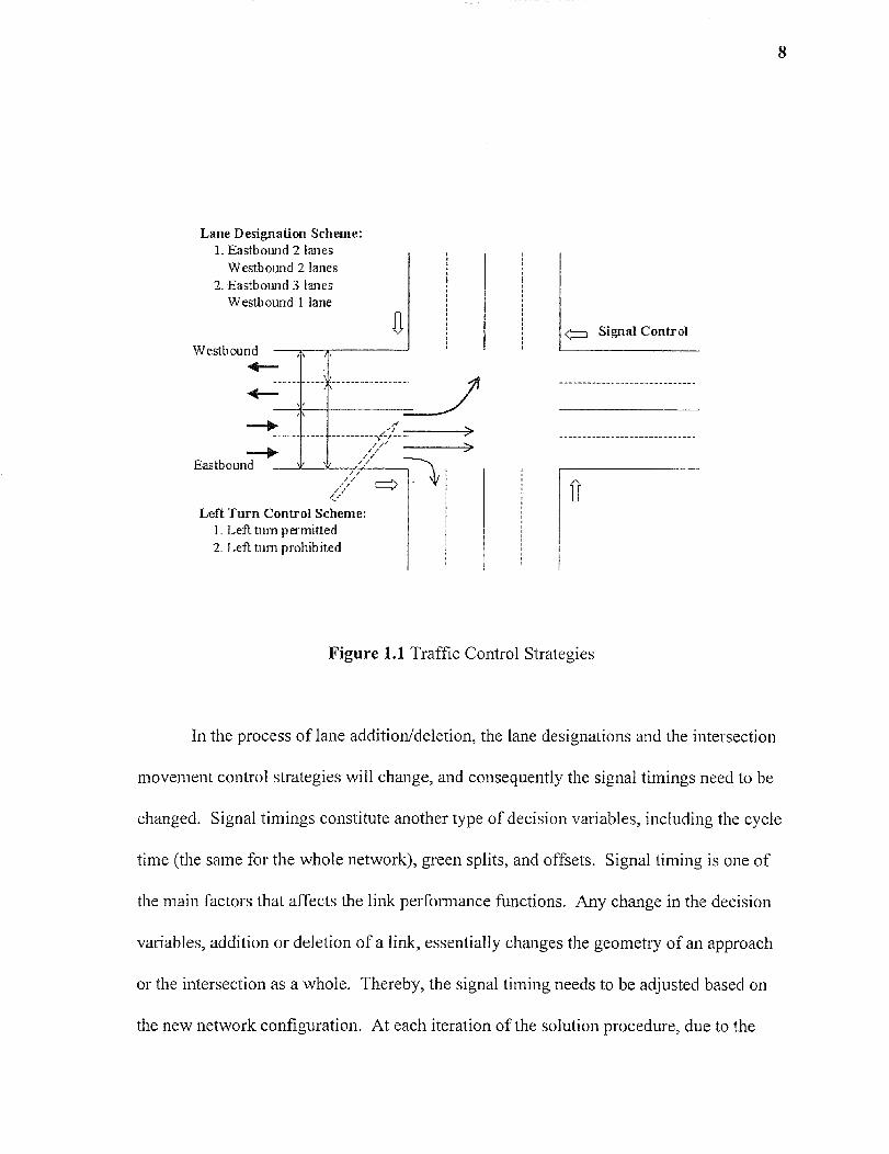
<-1 Signal Control
Lane Designation Scheme:1. Eastbound 2 lanes
Westbound 2 lanes2. Eastbound 3 lanes
Westbound 1 lane
Westbound
4—
Eastbound
Left Turn Control Scheme:1. Left turn permitted2. Left turn prohibited
ft
Figure 1.1 Traffic Control Strategies
In the process of lane addition/deletion, the lane designations and the intersection
movement control strategies will change, and consequently the signal timings need to be
changed. Signal timings constitute another type of decision variables, including the cycle
time (the same for the whole network), green splits, and offsets. Signal timing is one of
the main factors that affects the link performance functions. Any change in the decision
variables, addition or deletion of a link, essentially changes the geometry of an approach
or the intersection as a whole. Thereby, the signal timing needs to be adjusted based on
the new network configuration. At each iteration of the solution procedure, due to the
8
addition/deletion of links, the signal timing changes and consequently the link
performance functions need to be updated at each iteration. The last type of decision
variables is the link flow variable that is obtained by solving the lower level UE traffic
assignment problem in an UTNDP. Link flows are affected by lane designations,
intersection movement controls, and signal settings. The updates of lane designations
and intersection movement controls are based on the Simulated Annealing TABU Search
heuristic that is described in Chapter 3. Signal settings are obtained by solving a non-
linear programming model that includes capacity constraints that are dependent on the
link flows.
1.3 Research Objectives
The primary objectives of this dissertation are the formulation and development of a
heuristic search strategy to solve a transportation network design problem by optimizing
traffic control strategies in urban signalized networks. The specific objectives of the
problem are:
I) Formulate the traffic control optimizing strategy as an UTNDP model.
2) Develop a heuristic search strategy to solve the UTNDP
• Develop a traffic assignment procedure to find the flows on signalized network.
• Identify a signal optimization procedure.
• Perform computational experiments to demonstrate the feasibility and effectiveness
of the UTNDP search strategy on small size urban networks.
9
10
1.4 Overview
In Chapter 2, the literature review on both the formulation and solution algorithms of
NDP models is presented. The problem formulation is introduced first, followed by the
link performance functions that are used for estimating link travel times. Since the
UTNDP is a bi-level programming problem with the lower level problem as an UE traffic
assignment problem, literature on traffic assignment is also introduced, followed by the
algorithms for both the upper and lower level problems. The last section of Chapter 2
presents a review on network representation that is the basis of any network analysis. In
Chapter 3, the UTNDP methodology is outlined, which includes the bi-level model
formulation and the proposed solution strategy. In Chapter 4, the flowcharts and the
corresponding main subroutines of the heuristic search procedure are presented, including
the heuristic evaluation functions, and the updating criteria. In Chapter 5, numerical
experiments are presented on four test networks. Conclusions and recommendations on
future work are presented in Chapter 6.
CHAPTER 2
LITERATURE REVIEW
An UTNDP is a typical bi-level programming problem, where the upper level problem is
a 0-1 integer programming problem, and the lower level problem is a traffic assignment
problem. This literature review addresses both of these problems which are presented in
the following sections together with existing solution algorithms and heuristics.
Literature on performance functions (travel time functions) and network representations
that are critical to the formulation and solution of UTNDP models are also presented.
2.1 The Formulation of Network Design Problem
An NDP falls into the category of the Stackelberg game (17), which is a well-studied
field in operations research. Stackelberg games characterize a behavioral model of two
players. One player (the leader) wants to optimize a certain objective, and s/he knows
how the other player (the follower) will respond to any decisions s/he makes. If neither
player can improve his/her objective by unilaterally changing his/her decision, then an
equilibrium state is reached. Four important references on NDP are LeBlanc (1),
Magnati and Wong (14), Friesz (8) and LeBlanc and Boyce (4). Magnati and Wong (14)
provided an extensive review on both continuous and discrete NDP models. The
relationship between NDP and other transportation network analysis problems was also
discussed in their paper. Friesz (8) provided a comprehensive review on transportation
network design problems and discussed the research opportunities in this field. In the
next sections the formulation proposed by LeBlanc and Boyce (4) and LeBlanc (1) are
11
12
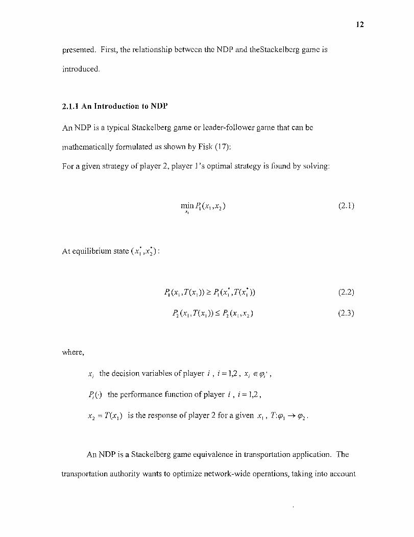
presented. First, the relationship between the NDP and theStackelberg game is
introduced.
2.1.1 An Introduction to NDP
An NDP is a typical Stackelberg game or leader-follower game that can be
mathematically formulated as shown by Fisk (17):
For a given strategy of player 2, player l's optimal strategy is found by solving:
min P1(x1,x2, )
(2.1)
At equilibrium state (.74,x;) :
(x,,T(x 1 )) >(P1x1* ,T(x1)) (2.2)
P2 (X i , T(x1 )) P2 (X i , ) (2.3)
where,
x, the decision variables of player i , i = 1,2 , x, E
P, 0 the performance function of player i , i = 1,2 ,
x_, = T(x 1 ) is the response of player 2 for a given x, , T:v 1 ç2.
An NDP is a Stackelberg game equivalence in transportation application. The
transportation authority wants to optimize network-wide operations, taking into account
13
the travelers' response to a specific network configuration. The transportation authority
plays the leader role, while the travelers play the follower role. In this UTNDP, the
transportation authority's (the leader) problem is to minimize the network-wide total
travel time by optimizing traffic control strategies such as left turn additions/deletions,
lane designation controls, and signal setting optimizations. In the UTNDP model, the
traffic control strategy variables (the upper level decision variables) are equivalent to the
x, variables in the Stackelberg game, and the link traffic flow variables (the lower level
decision variables), which are the responses of travelers to a given network configuration
and traffic control strategies, are equivalent to the x, variables in the Stackelberg game.
Similar to the UTNDP, optimal signal setting problems are also identified as
Stackelberg games (17,38). The decision variables in a signal setting problem include
cycle lengths, green splits, and offsets of adjacent intersections. Any changes of signal
setting parameters result in changes of link performance functions, and they cause
changes in traffic flow distribution patterns. Allsop (34) pointed out that the effect of the
signal setting on flow distribution patterns should be taken into account in the traffic
assignment process. In addition, Heydecker (18), Smith (33), Cantarella et al. (35) and
Yang et al. (40) gave similar suggestions. The combined signal setting and traffic
assignment problem is also referred to as equilibrium network traffic signal setting that
can be solved by two approaches, global optimization models and iterative procedures.
The global optimization models are continuous NDP models. Usually, among all signal
setting parameters (i.e. cycle lengths, green splits, and offsets), only green splits are
treated as decision variables, where all other parameters are assumed to be given. These
models minimize network-wide travel time in terms of green splits and traffic flows
14
under a UE traffic flow pattern. There are two main disadvantages associated with these
global optimization models. First, there are no existing efficient solution algorithms;
second, this formulation ignores signal coordination among adjacent intersections that
has significant influence on network performance. Cantarella et al. (35) proposed an
iterative procedure named ENETS (Equilibrium Network Traffic Signal Setting) which
has two consecutive signal setting steps, the single intersection signal setting step and the
network coordination step. The iterative procedure allows all signal setting parameters to
be treated as decision variables and has less computational requirements. However, the
convergence of this procedure can not be guaranteed (20,37).
Since traffic engineers often decide not only to change the signal settings but also
change the lane designations and the intersection movement controls, an UTNDP and an
equilibrium network traffic signal setting problem often intertwine with each other. In
this dissertation, the UTNDP is formulated in a way that it includes the equilibrium
network traffic signal setting problem as an essential step in the whole procedure to
optimize the signal settings and the network configuration simultaneously.
2.1.2 A Bi-Level Programming Model by LeBlanc and Boyce
There are two types of decision makers in a Stackelberg game, the facility authority,
which is also viewed as the upper level decision makers, and the facility users, who are
viewed as the lower level decision makers. The interaction between these two types of
decision-makers requires a formulation that can reflect the bi-level nature of a
Stackelberg game such as an UTNDP. In 1986, LeBlanc and Boyce (4) formulated the
UTP as a bi-level programming model as follows:
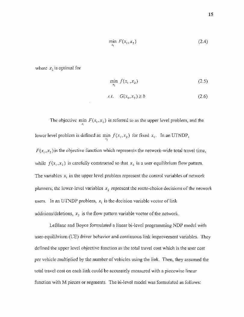
where x„ is optimal for
15
min F(x1, , x, )
(2.4)
min f(x1x2)
(2.5)
Si. G(x1 , x2 b (2.6)
The objective min F(x , is referred to as the upper level problem, and thex1
lower level problem is defined as min f(x1,x2 ) for fixed x1 . In an UTNDP,1 2
F(x1 ,x2 ) is the objective function which represents the network-wide total travel time,
while f(x1,x2) is carefully constructed so that x2 is a user equilibrium flow pattern.
The variables x1 in the upper level problem represent the control variables of network
planners; the lower-level variables x2 represent the route-choice decisions of the network
users. In an UTNDP problem, x, is the decision variable vector of link
additions/deletions, x, is the flow pattern variable vector of the network.
LeBlanc and Boyce formulated a linear bi-level programming NDP model with
user-equilibrium (UE) driver behavior and continuous link improvement variables. They
defined the upper level objective function as the total travel cost which is the user cost
per vehicle multiplied by the number of vehicles using the link. Then, they assumed the
total travel cost on each link could be accurately measured with a piecewise linear
function with M pieces or segments. The bi-level model was formulated as follows:
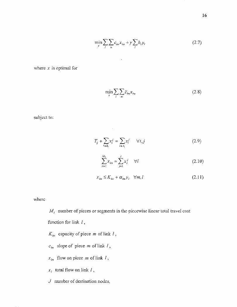
16
min ci„,x1„, + r 13,y, (2.7)m
where x is optimal for
min Z e-IntX Im (2.8)
m
subject to:
+> =t
Vi,j (2.9)
J
x 1,,, (2.10)m=1 j=1
x 11 K + a ImY V171, 1
(2.11)
where
M, number of pieces or segments in the piecewise linear total travel cost
function for link 1,
K,,,, capacity of piece m of link 1,
C1m slope of piece m of link 1,
x,,,, flow on piece m of link 1,
total flow on link 1,
J number of destination nodes,

17
..r" flow on link / with destination j,
T required number of trips between origin node i and destination node j ,
A, set of links pointing out of node i (after node i),
B, set of links pointing into node i (before node i),
alm,„ are exogenously specified parameters with I a1m =1
, the unit cost of improvements on link 1,
. 1„, the slopes of the piecewise linear integrals of the user-cost functions,
y, decision variable on link 1,
y constant.
Bard (21) has shown that any linear bi-level program can be solved by solving a single
linear program and then by iteratively modifying the objective function and resolving it.
When the network is within a reasonable size, the piecewise linear bi-level programming
model should yield an exact solution. However, for larger networks with thousands of
nodes or many linear pieces per link, the model can not be solved directly. In their paper,
LeBlanc and Boyce suggested an efficient solution procedure for larger networks. They
suggested using an equivalent optimization model in place of the linear program in
Bard's algorithm. This equivalent optimization model can be solved very efficiently
using the Frank-Wolfe algorithm. LeBlanc and Boyce's work was the first exact solution
for the continuous NDP at that time. However, their model can only be applied to small
size real world networks with continuous decision variables.
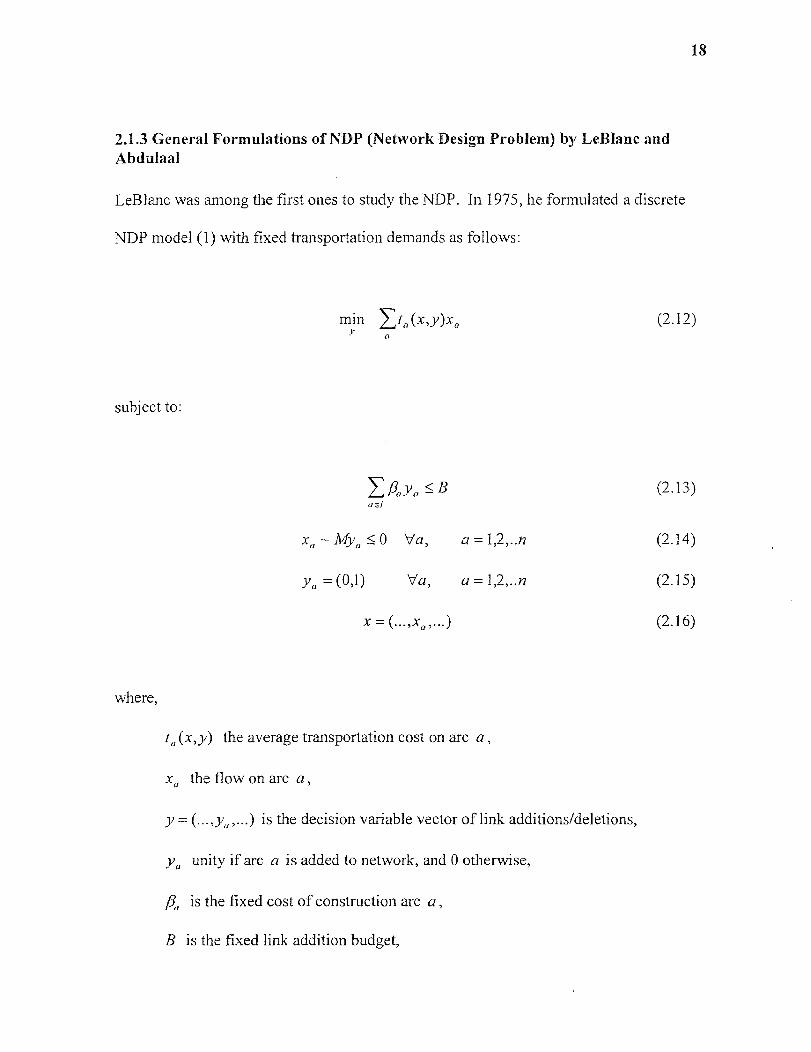
2.1.3 General Formulations of NDP (Network Design Problem) by LeBlanc andAbdulaal
LeBlanc was among the first ones to study the NDP. In 1975, he formulated a discrete
NDP model (1) with fixed transportation demands as follows:
min „(x,y)x, (2.12)fl
subject to:
EBaYa (2.13)ael
Xa — My, :5_0 Va, a =1,2,..n (2.14)
ya = (0,1) Va, a = 1,2,..n (2.15)
x=(...,x,,...) (2.16)
where,
ta(x,y) the average transportation cost on arc a,
x, the flow on arc a,
is the decision variable vector of link additions/deletions,
y„ unity if arc a is added to network, and 0 otherwise,
A, is the fixed cost of construction arc a,
B is the fixed link addition budget,
18
M is a large constant,
I is the set of arcs considered for addition to the network,
n is the number of links in the network.
This is also a bi-level program. The objective function a (x,y)xa is the total
19
travel time of the network. Constraint (2.13) is the budget constraint; (2. 14) prohibits
flow on links that are prohibited. The constraint (2.16) is the lower level of the bi-level
program, which can be obtained from an equivalent minimization problem or a VIP.
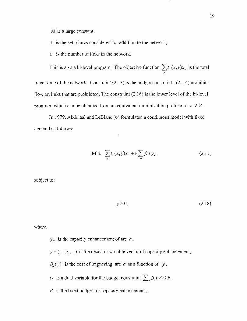
In 1979, Abdulaal and LeBlanc (6) formulated a continuous model with fixed
demand as follows:
Min. E t„ (x,y)xa+wEBa(y), (2.17)
subject to:
y 0, (2.18)
where,
ya is the capacity enhancement of arc a,
y is the decision variable vector of capacity enhancement,
(y) is the cost of improving arc a as a function of y,
w is a dual variable for the budget constraint Ea 13 a (y)_. B,
B is the fixed budget for capacity enhancement,
20
All other notations are the same as the discrete model.
In this model, the budget constraint was put into objective by introducing
Lagrangen dual variable w.
2.2 Link Performance Functions
Link performance functions, also known as link travel time functions, are mathematical
models used to estimate the link travel times, as a function of traffic flow, geometric
characteristics of the modeled facility and intersection signal settings and control
strategies (13,31). The shape of performance functions is important because they have
significant impact on both the computational tractability of the UTNDP and the existence
and uniqueness of the solutions of the UE problem at the lower level. In general, the link
travel time functions for controlled intersections consist of two components: the cruise
time on the link and intersection delay. Link cruise time is the time of a vehicle travels
from the beginning to the end of a link. Intersection delay considers the time a vehicle is
delayed due to the control for the specific movement that a vehicle is trying to perform.
2.2.1 The BPR Type Curves (55)
The most well known link travel time function is the Bureau of Public Roads (BPR)
curve. The BPR curve is more appropriate for freeway links rather than signalized
streets, because it doesn't reflect the impact of delays caused by signal settings and
turning movement controls at intersections. The BPR curve is presented below:
21
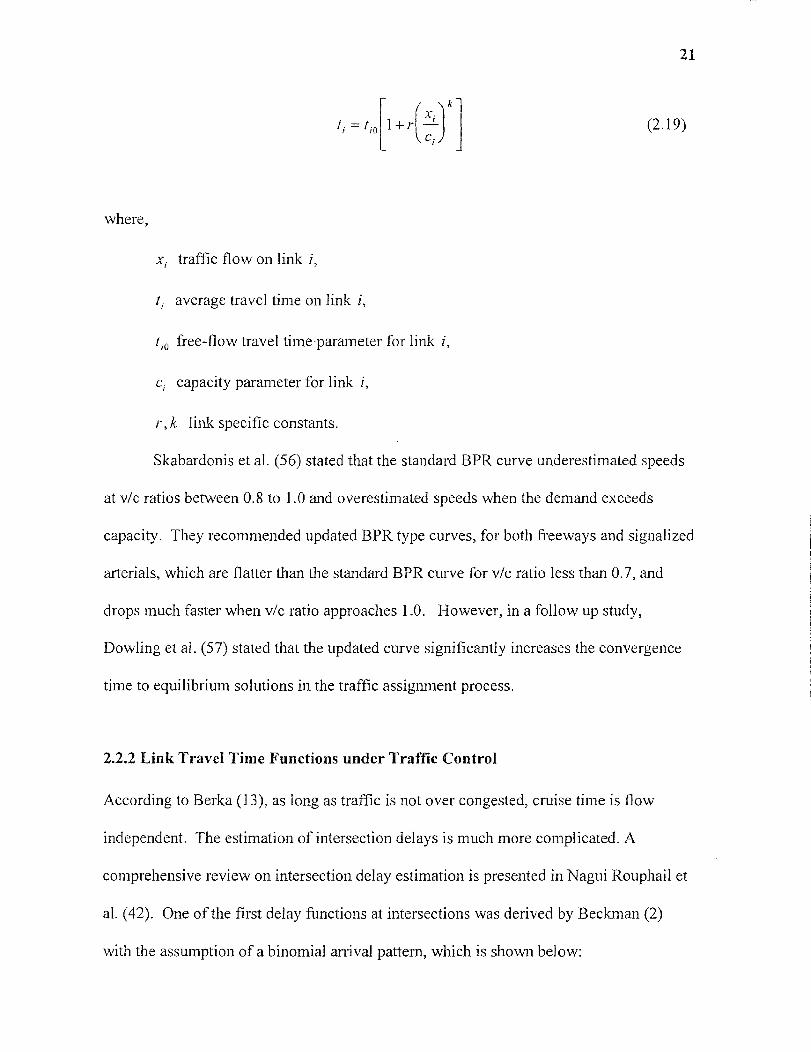
( xiti = 1 10 1 +r
ci(2.19)
where,
x, traffic flow on link i,
t, average travel time on link i,
t i© free-flow travel time parameter for link i,
c, capacity parameter for link 1,
r,k link specific constants.
Skabardonis et al. (56) stated that the standard BPR curve underestimated speeds
at v/c ratios between 0.8 to 1.0 and overestimated speeds when the demand exceeds
capacity. They recommended updated BPR type curves, for both freeways and signalized
arterials, which are flatter than the standard BPR curve for v/c ratio less than 0.7, and
drops much faster when v/c ratio approaches 1.0. However, in a follow up study,
Dowling et al. (57) stated that the updated curve significantly increases the convergence
time to equilibrium solutions in the traffic assignment process.
2.2.2 Link Travel Time Functions under Traffic Control
According to Berka (13), as long as traffic is not over congested, cruise time is flow
independent. The estimation of intersection delays is much more complicated. A
comprehensive review on intersection delay estimation is presented in Nagui Rouphail et
al. (42). One of the first delay functions at intersections was derived by Beckman (2)
with the assumption of a binomial arrival pattern, which is shown below:
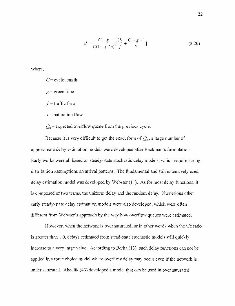
22
d C - a 00 C - g 1
C(1— f I s(2.20)
where,
C= cycle length
g = green time
f = traffic flow
s = saturation flow
Qo = expected overflow queue from the previous cycle.
Because it is very difficult to get the exact form of Q 0 , a large number of
approximate delay estimation models were developed after Beckman's formulation.
Early works were all based on steady-state stochastic delay models, which require strong
distribution assumptions on arrival patterns. The fundamental and still extensively used
delay estimation model was developed by Webster (11). As for most delay functions, it
is composed of two terms, the uniform delay and the random delay. Numerious other
early steady-state delay estimation models were also developed, which were often
different from Webster's approach by the way how overflow queues were estimated.
However, when the network is over saturated, or in other words when the vie ratio
is greater than 1.0, delays estimated from stead-state stochastic models will quickly
increase to a very large value. According to Berka (13), such delay functions can not be
applied in a route choice model where overflow delay may occur even if the network is
under saturated. Akcelik (43) developed a model that can be used in over saturated
23
situations. Based on extensive field studies, Reilly et al. (44), modified Akcelik's
formula, and Reilly's equation was further modified by Roess et al. (45), and the
improved model is applied by the 1997 HCM (46).
Another limitation of steady-state stochastic models is that they do not reflect the
coordination of adjacent intersections. None of the above mentioned studies incorporated
offsets in their models. In a transportation network, with coordinated signals, offsets are
critical decision variables. Network-wide signal setting problems are characterized by
the optimization of offsets. To optimize signal coordination, offsets must be incorporated
into the link travel time estimation function as independent variables. These types of
functions are also known as delay-offset functions. The only closed form delay-offset
function was provided by Gartner (38).
One of the most important contributions to the modeling of link travel time
estimations with turning movement delays was done by Berka et al. (13). For the
estimation of cruise time, Berka et al. obtained a formula by regression from the
measurement data of the 1985 HCM. For the estimation of intersection delays, the
models were classified by roadway and intersection types. The roadway types considered
are arterials, collectors, freeways and tollway facilities. They further divided the arterials
and collectors into signalized intersections, major/minor priority intersections and all-
way-stop intersections. The models for arterials and collectors are the most complicated
ones, because these types of roads are located in urban areas, and their control, geometric,
and flow characteristics are more complicated than other types. Arterial and collector
intersections were classified into 12 categories according to the intersection control, the
intersection layout and the intersection geometry. Their analysis was based on a lane
24
group basis, except for the left turn lane that was analyzed separately, which is consistent
with the 1997 HCM (46). The intersection delay analysis consists of four modules: lane
flow estimation, saturation flow analysis, signal timing procedure and delay function
estimation. These modules are mutually dependent, requiring an iterative procedure to
obtain consistent results. Compared with BPR curve based travel time estimation
method, Berka et al.'s procedure are more appropriate forcontrolled facilities. However,
one important traffic flow factor, the progression, was ignored in their procedure.
2.2.3 Signal Timing Optimization
One of the critical elements of the procedure proposed in this study is the signal timing
optimization. By its nature, this is a rather complicated problem. For isolated
intersections, the fundamental work has been done by Webster (3). Because of its simple
form, it is widely used in transportation network optimization models. However, the
discrepancy between the global optimal objectives of transportation network optimization
problems and the non-global nature of isolated intersection signal setting approach
requires a different signal optimization approach than Webster's. The network-oriented
signal setting model was first introduced by Little (47), using the bandwidth
maximization method. However, Little's method, and all other similar maximum-
bandwidth methods thereafter, did not take into account traffic flows, which are widely
accepted as one of the main factors affecting signal optimization in networks. In the mid.
60's, flow-dependent signal optimization packages were developed in the U.S., including
SICTRID (48) and STOOP (49). However, these packages failed to consider loop
constraints, which require offsets and greens on a loop to add up to cycle length
25
multiplied by an integer. In Britain, combination methods (51) were developed by the
Road Research Laboratory to calculate optimal offsets for series-parallel networks.
Later, the Road Research Laboratory developed another signal optimization method
TRANSYT. Both the combination methods and the TRANSYT used the critical
intersection approach to calculate the cycle length. These methods calculated the cycle
length of the most congested intersection in a network, and then made it the cycle length
of all the intersections in the network, which may not be optimal for a network situation.
Simultaneous optimization of all decision variables: green splits, cycle length and offsets
was first introduced by Gartner (50) in 1975. He used a mixed integer linear
programming model to optimize all variables. The objective function of Gartner's model
needs to be linearized, that increases both the number of variables and the number of
constraints, and makes it very difficult to be applied to real size transportation networks.
Some of the existing commercial signal optimization software is discussed next.
TRANSYT-7F is the most popular one for networks, while PASSERII-90 is popular for
signal optimization for arterials. TRANSYT-7F was developed as part of the national
signal timing optimization project (NSTOP). It is a macroscopic simulation software that
simulates traffic in small time increments (39). The quality of progression is reflected in
TRANSYT-7F by a platoon dispersion model that is capable of being used to simulate
traffic dispersion realistically. TRANSYT-7F uses Webster's method to estimate delays
which consists of three parts, uniform delay, random delay and an empirically adjustment
factor. The TRANSYT-7F input includes network configuration data, timing data,
saturation flow data, speed data and volume data. The output of TRANSYT-7F includes
cycle lengths, phase lengths, intersection delays, total travel time, average speeds, fuel
26
consumption etc. For a given cycle length, TRANSYT-7F can be used to optimize phase
lengths and offsets. The program can evaluate a range of cycle lengths and select the best
one. The objective function used in the optimization process is the performance index
(PI), which is defined by the users. The most commonly used PI is a weighted
combination of stops and delays, i.e.: PI = delay + "k" *stops, where k is the stop penalty.
Another well known software is PASSER 11-90, which was developed by Texas
Transportation Institute of the Texas A&M University System. PASSER 11-90 is a
computer program that can assist traffic engineers in analyzing both individual signalized
intersections and progression operations along an arterial street (36). PASSER 11-90 can
be used to optimize progression signal timing. It can optimize up to 20 intersections
along the arterial. PASSER 11-90 can examine a range of cycle lengths and select the one
that provides the best progression. It uses the Webster's method to calculate cycle
lengths and green splits. The input of PASSER 11-90 includes network configuration
data, speed data, volume data, timing data and control data. The output of PASSER 11-90
includes cycle lengths, efficiency (the average fraction of the cycle used for progression),
average speed through system, total travel delay, total fuel consumption, intersection v/c
ratios, phase time, intersection delays, and level of service. In the optimization process,
the efficiency is used as the objective function.
27
2.3 The Lower Level Problem (Traffic Assignment Problem)
2.3.1 The Variational Inequality Based Formulation
In 1980, Dafermos first pointed out that the equilibrium conditions are equivalent to a
variational inequality problem (VIP) formulation. Dafermos' formulation (23) is
described below:
Find (x,T) E Q , such that:
c(x * )(x — x . ) — 0(T * )(T — T) > 0 V (x ,T E Q) (2.21)
o = {(x,T): f = V (i , j); x a jar p ; 0;T 0) (2.22)P EP u
where:
x = (...,xa ,...) denotes link flows,
f =(...,f,,...) denotes path flows,
p if link a is on path p ,
= o otherwise,
c(x) = (...,c, (x),...)where ca (x) denotes average travel cost on link a ,
T= (. ..,T ,...) where 7; denotes O-D flow for 0-D pair (i,j),
0 = (. . . 4(T),...) where 0, (T) is the inverse travel demand function for O-D pair
(i,j).
28
Existence conditions for this VIP are that c(x) and — 0(T) must be continuous
and T(u) (u is the user equilibrium travel time) are bounded from above. Uniqueness
conditions are that c(x) and — 9(T) are strictly monotone increasing. The variational
inequality mathematical formulation is more general as it describes the UE conditions
directly, and it applies to both symmetric and asymmetric cases.
2.3.2 The Mathematical Programming Formulation (The Symmetric TrafficAssignment Problem)
If link interactions are symmetric, the traffic assignment problem can be formulated as a
mathematical programming problem (12). However, the mathematical programming
formulation is not intuitive to the UE conditions, and it can only be applied to symmetric
link interaction case only. For the user equilibrium conditions, Beckman et al.'s
formulations is as follows:
Min. z= a(t) dt (2.23)(1=1
subject to:
f rsk Vk,r,s (2.24)
fkrs > 0 Vk,r,s (2.25)
x. = E frsk ak (2.26)r s k
29
where,
x„ is the flow on link a,
x=(...,x„,...) is the link flow vector,
f1 is the flow on path k of O-D pair rs,
qr is the travel demand between O-D pair rs,
ta(x) is the travel time function (performance function) of link a,
(5:2 =1 if path k of O-D pair rs is on link a, and 0 otherwise.
The solution to the above mathematical problem produces an equilibrium traffic flow
pattern.
For the system optimal formulation, the objective function is to minimize the total
travel time that is presented below.
min z(x) = x,t,(x,) (2.27)
subject to (2.24)-(2.26).
Both the UE and the SO formulations can be solved by the Frank-Wolfe
algorithm, which was originally proposed by LeBanc et al. (2). According to Sheffi (5),
solving the SO formulation is equivalent to solving an UE program in which the cost
functions t, (x, ) are replaced by the corresponding marginal cost functions (x,).
Tj(xi) = ti(xi)+ xi (2.28)
30
2.4 Solution Algorithms for the Lower Level Problem(The Traffic Assignment Problem)
2.4.1 Solution Algorithms for the Symmetric Traffic Assignment Problems
In the following sections, two algorithms that are used to solve the symmetric traffic
assignment problem are presented. The first one is the Frank-Wolfe algorithm (7), and
the second one is a path based gradient projection (GP) algorithm.
Frank-Wolfe algorithm is the most commonly used algorithm in solving
symmetric traffic assignment problems. Frank and Wolfe (7) originally suggested the
algorithm, and it is also known as the convex combination method. The Frank-Wolfe
algorithm is a feasible descent method that is based on a linear approximation of the
objective function at each iteration. The descent direction is found by optimizing a linear
approximation of the objective function. The move size along the descent direction is
found by minimizing the approximated objective function. The Frank-Wolfe algorithm
has been widely used in traffic assignment problems because of the equivalence between
the descent direction finding step and the all-or-nothing assignment. The all-or-nothing
assignment requires repeated applications of one-node-to-all-nodes shortest path routine.
This shortest path routine is the main computational requirement of Frank-Wolfe
algorithm.
The Gradient Projection (GP) algorithm is a path-based algorithm. Path-based
algorithms have not drawn enough attention by transportation researchers because the
algorithms require very large computer memory. The basic idea behind the GP algorithm
is that for any feasible solution a better solution can be found by moving along the
negative gradient direction. The negative gradient direction is calculated with respect to
the flows on the non-shortest paths, and a move size is found by using the second

31
derivatives with respect to these path-flow variables. Jayakrishnan et al. (28) have
presented an application of the GP algorithm. Their research suggests that the memo y
problems of the GP algorithm can be addressed effectively by existing computer
hardware and software. They have also demonstrated that the computational
performance of the GP over the Frank-Wolfe is substantial.
2.4.2 Solution Algorithms for Asymmetric Traffic Assignment Problems
Given a link flow vector x = (x 1 ,...,x„) and the link travel time vector
t(x) (t, (x),...,t„(x)), the asymmetric traffic assignment problem can be formulated as a
variational inequality problem (VIP) as follows:
Find x . E X such that t(x . )(y — x . ). 0 , Vy e X
To solve asymmetric UE traffic assignment problems, a sequence of symmetric
problems must be defined to approximate the asymmetric problems. Friesz (8)
summarized the available solution algorithms and grouped them into three categories:
1. Linearization methods
In a linearization algorithm, at each iteration 4•) is approximated by a linear
approximation t(k)(x).
1(k) (x) t(x(k)) A(X (k) - x (k) ) (2.29)
32
Then the VIP is solved: t (k) ) • (y — 0 , Vy E X to get x (" ) until certain
termination criterion is satisfied. When A(x) is chosen as a symmetric positive
definite matrix, the algorithm is called the projection method (23).
2. Diagonalization methods (6,15)
In the diagonalization algorithm (also known as nonlinear Jacobi methods), at
each iteration a diagonalization of function t() is performed to obtain:
t (k) (x,x(k) =J J (2.30)
Then the VIP is solved: t(k))(x*)•(y— 0 Vy E X to get x (" ) until certain
termination criterion is satisfied.
Sheffi (5) proposed a streamlined version of the diagonalization algorithm by
performing only one iteration of the symmetric UE sub-problem. Mahmassani and
Mouskos (15) conformed that the sub-problem need only be solved approximately, by
performing only a few Frank-Wolfe iterations from one to four. They suggested that for
each problem trial tests should be conducted to determine the optimal number of
iterations.
3. Simplicial decomposition methods (22)
In the simplicial decomposition algorithm, the feasible set is represented by
extreme points that are updated at each iteration. These extreme points form a convex
simplified feasible set that makes the problem easier to solve.

33
2.5 Search Procedures of the Upper Level Problems
Maganati and Wong (14) summarized the solution methodologies for discrete NDP. The
search strategies can be grouped into two categories, exact search strategies and heuristic
search strategies. The most commonly used exact search method of solving the discrete
NDP is the well-known branch and bound technique of integer programming. One of the
first studies conducted in this area is the work by LeBlanc (1). He formulated the budget
constrained discrete equilibrium NDP as program (2.12)-(2.15), and proposed a branch
and bound solution algorithm with SO results as the lower bound. The branch and
bound search procedure was also adapted by Hoang (19) and Dionne and Florian (16).
Heuristic search strategies can be divided into two categories: informed and
uninformed. The informed search uses information gathered from previous states to
guide the search of the next state. The uninformed search proceeds in a way with a
predetermined strategy that is independent of the intermediate information from the
previous states. The informed strategy is more interesting, because the uninformed one is
rather inefficient for large-scale problems. Recent advances in heuristic search strategies
of solving large-scale combinatorial problems can be classified into three groups: the
TABU search, the simulated annealing and the neural network methods. The next two
sections present the principal characteristics of the TABU search and the simulated
annealing methods.

34
2.5.1 TABU Search
TABU search was developed by Glover (24-26). The first application of TABU search to
solve the UE single class discrete UTNDP was developed by Mouskos (3). The principle
elements of TABU search are the followings:
• TABU lists: TABU lists contain a set of moves that are not permitted to be
undertaken during a certain number of iterations during the search. The primary
purpose of these lists is to move the search away from the current search space and
reduce the risk of cycling.
• Heuristic evaluation functions: The heuristic evaluation function is used to evaluate
all available moves and the move where the best value is selected to move from one
solution state to another.
• Aspiration level: The aspiration level is used to override the TABU status of a move
if its evaluation function reaches a certain value (aspiration level).
• Strategic oscillation: Strategic oscillation is often used to search the space around the
boundaries of the constraints. It serves as a sensitivity analysis tool to the search.
• Intermediate memory function: Intermediate memory function rewards good moves
to intensify the search around good solutions.
• Long term memory function: Long term memory function is used to diversify the
search into another place of the solution space.
• Dominant and deficient moves: A move is called a dominant move if when a TABU
condition prevents this move, it also prevents a set of associated moves. A move is
called a deficient move if it provides no possibility for an improved solution.

35
TABU search has been applied in different types of problems, such as the job
scheduling problem, the computer channel balancing problem, and the travel salesmen
problem. Mouskos (3) successfully implemented TABU search in a single user class
discrete transportation equilibrium network design problem. He used five small
experimental networks to test the algorithm, where the optimal solutions were obtained in
less than 500 iterations. He also tested his method on three medium size networks, where
Good solutions were also obtained.
2.5.2 Simulated Annealing Procedure
The basic search strategy follows the Metropolis algorithm (32). The Metropolis
algorithm was motivated by an analogy to the physical annealing process of solids. In
condensed matter physics, annealing is known as a thermal process for obtaining a low
energy state of a solid in a heat bath. If the cooling process is conducted in such a way
that at every temperature a thermal equilibrium of the object can be reached, then the
material internal energy will be reduced greatly or even reduced to the minimal energy
state. A thermal equilibrium is reached at a temperature T if the probability of being in
state i with energy E, is governed by a Boltzman distribution:
exp(— k i3 T)
(2.31)EE exp
kBT)

36
where k B is the Boltzman constant. The basic idea of this algorithm is modeling the
transition from the current state to the next state so that the Boltzman distribution can be
achieved. The application of this algorithm in UTNDP requires the identification of three
elements: move generation, acceptance criteria and cooling schedule. The move
generation mechanism is presented in the previous paragraph. The acceptance criterion is
constructed as:
P {accept j} = f (i)— f WI f f(i)
c f (j)> f (i)(2.32)exp
where
Pe {accept j} is the acceptance probability of state j,
f (i), f (j) is the network-wide total travel time of state i and j, respectively,
c E R+ denotes the control parameter.
The cooling schedule defines the number of transitions generated under a control
parameter value and the changing plan of this control parameter. The cooling schedule
determines the speed of convergence of the algorithm.
For a combinatorial optimization problem, the objective function plays the same
role as energy does for the annealing of the physical system. The control parameter plays
the same role as temperature does. The solution process of a combinatorial optimization
problem can be viewed as a simulated annealing process, evaluated at decreasing values
of the control parameter. Simulated annealing algorithm was applied to combinatorial
optimization problems by Kirkpatrick et al. (29). The identification of three elements:
37
the generation mechanism, the acceptance criteria and the cooling schedule are critical to
the application of the simulated annealing in combinatorial problems.
The simulated annealing algorithm has been used in job shop scheduling
problems by Matsuo et al. (30). Friesz et al. (9) formulated a continuous NDP with
variational inequality constraints and proposed a simulated annealing algorithm to solve
it. Their conclusion was that the simulated annealing algorithm was superior to other
commonly used algorithms in accuracy, but it was very computationally demanding.
Only important problems, which require accurate solutions, justified the use of the
simulated annealing algorithm. Zeng (44) used a combined simulated annealing and
TABU search algorithm (SA-TABU) in solving a discrete UTNDP. He conducted
numerical tests on the same five networks (from 18 to 38 links) used by Mouskos (3).
Three sets of tests were performed, the first set used the traditional TABU search method,
the second set used simulated annealing method, and the last set used the combined
simulated annealing and the TABU search algorithm (SA-TABU). These three methods
were also tested on three larger networks (1206, 2022, and 3026 decision variables). The
SA-TABU search strategy was found to be an efficient and robust alogorithm in
providing "good" solutions to the problem. Compared with the conventional simulated
annealing procedure, the SA-TABU directed its search faster toward a set of "good"
solutions, and was more applicable in solving large scale problems.
2.6 Network Representation
Network representation is important both to the model formulation and the algorithm
design. A network needs to be constructed in an appropriate way so that it can represent
38
all the major features of an operational transportation network. Detailed representation
method leads to good quality results, however, it is often at the price of an over
complicated network representation which significantly increases the computational
burden. For example, to represent the turning movements, additional abstract links
should be added for each movement at the intersections. The forward star structure is the
most widely used data structure to represent a transportation network. In the following
sections, three network representation methods are introduced.
2.6.1 The Conventional Network Representation
In conventional route representation, each intersection is represented by a node, and each
road segment is represented as an approach link. For details, see Sheffi (5). Turning
movements can not be represented by this method. Travel time in this representation are
functions of road segment geometry and traffic flows, they are not defined in terms of
turning movement attributes.
2.6.2 The Expanded Intersection Representation
For some transportation network studies, turning movements are very important. For
example, in urban areas, the cruise time spent on an approach link is often much less than
the delays occurred at intersections. These delays are due to either signal settings or
conflicting traffic flows when turning movements are involved. The turning movements
in urban signalized networks can not be ignored, and should be represented appropriately.
Under the expanded intersection representation, each turning movement is
represented by an abstract link that is called an intersection link. The links connecting
adjacent intersections are called non-intersection links, or regular links. Because of the
network expansion, it requires increased computational time and computer memory.
2.6.3 Extended Forward Star Structure (EFSS)
In 1996, Ziliaskopoulos et al. (41) developed a method in a more economical, compact
and manageable way to represent networks. His study is an extension to the commonly
used forward star structure with a network representation method that can be used to
represent intersection movements, the associated delays and movement prohibitions.
39

CHAPTER 3
METHODOLOGY
In this chapter, the UTNDP is formulated as a bi-level mathematical program. Then the
link performance function estimation model is presented, followed by the signal setting
model. Next, the UE diagonaliztion algorithm is presented, which is adopted to solve the
asymmetric interactions between link flows in signalized networks. This chapter
concludes with a description of the heuristic used to solve the UTNDP bi-level program
that employs a combined Simulated Annealing and TABU Search (SA-TABU) strategy.
3.1 Formulation
The UTNDP is formulated as a typical bi-level programming problem where the upper
level problem represents the choices of transportation planners, and the lower level
problem represents the choices of the travelers in selecting their routes. The upper level
problem includes network configuration and signal setting optimization. Network
configuration optimization includes lane designation controls and intersection turning
movement controls, which are integrated into the UTNDP model as discrete decision
variables. Signal setting optimization includes the cycle time, offsets and greensplits, all
of which are continuous variables in the UTNDP. The UTNDP formulation is presented
next.
40
41
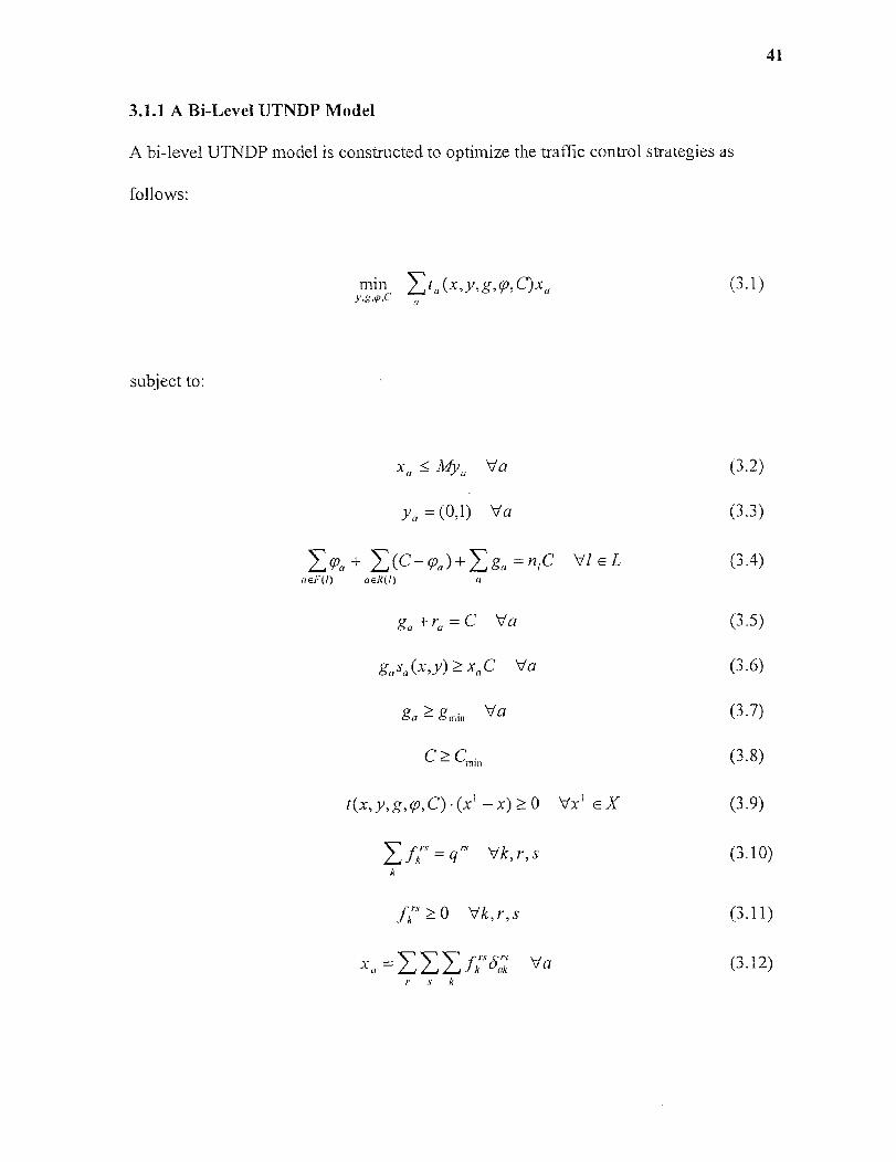
3.1.1 A Bi-Level UTNDP Model
A bi-level UTNDP model is constructed to optimize the traffic control strategies as
follows:
min (3.1)y,g,o,Ca
subject to:
Mya Va (3.2)
= (0,1) Va (3.3)
1g), +E (C- - ca,)+Ega = n I CV/ E L (3.4)aeF,(I) aeR(I) (I
g, +r„ = C Va (3.5)
gasa(x,y) xaC Va (3.6)
Va (3.7)
C Cmin (3.8)
t(x, y, g,q),C) • (x l — 0 eX 1 E X (3.9)
E fkrs = qrs V k,r, s (3.10)k
fk' 0 Vk,r,s (3.11)
=III fkrs. qakrs Va (3.12)
r s k

where
42
xa is the flow on link a,
x=(...,xa ,...) is the link flow vector,
ya is the network configuration decision variable, unity if link a is added to the
network, and 0 otherwise,
y = (..., y (1 ,...) is the network configuration decision variable vector,
ga is the green split on link a,
g = (...,g 2 ,...) is the green split vector,
g is the minimum green split,
yoa is the offset on link a, with respect to the upstream intersection,
q = is the offset vector,
C is the network-wide cycle length,
• is the minimum cycle length,
f, is the flow on path k of O-D pair rs,
q" is the travel demand between O-D pair rs,
t(x,y,g,q,C)=(...,ta(x,y,g,q,C),...) is the travel time function vector,
M is a large constant,
(Ks = 1 if path k of O-D pair rs is on link a, and 0 otherwise,
1 is the set of links that form a loop,
L = {1} is the set of all the loops,
F(1) is the set of forward links in 1,
R(1) is the set of backward links in 1,

43
nl is the integer loop constraint multiplier,
sa(x,y) is the saturation flow rate on link a.
Program (3.1)-(3.8) represents the upper level problem of an UTNDP. Function
(3.1) is the objective function which represents the network-wide total travel time (travel
time includes intersection delays hereafter). Constraint (3.2) prevents flows on turning
movements that are not allowed. Signal setting related constraints are represented in
(3.4)-(3.8) and are explained in detail in section 3.1.4.
Program (3.9)-(3.12) defines the traffic assignment, the lower level problem. The
VIP constraint (3.9) defines the user equilibrium (UE) traffic conditions. Constraint
(3.10) is the flow conservation constraint, constraint (3.11) is the non-negativity
constraint, and constraint (3.12) is the incidence relationship between link flows and path
flows. Also, note that link performance functions (link travel time functions)
(x, y,g,q,C) are functions of link flows x, network configuration variables y, and
signal setting variables g, q, and C. The travel time on a subject link depends not only
on the flow or the link itself, but also on the flows on other links and signal setting
variables.
The objective of this UTNDP model is to optimize traffic control strategies so that
the UE network-wide total travel time is minimized. At the upper level, transportation
planners decide lane designation controls, intersection movement controls and signal
setting controls. At the lower level, travelers choose their route individually, so that at
the equilibrium state the UE conditions are satisfied. There are three types of decision
variables. The upper level decision variables include network configuration variables y
and signal setting variables g, q, and C. The network configuration variables are used
44
to represent whether certain turning movements should be prohibited/permitted at some
intersections, or whether lane designations should be rearranged and how they should be
rearranged. The signal setting variables represent how signal splits and offsets are
allocated to each intersection and how long the network-wide cycle length should be.
The lower level traffic flow variables x represent the link flows at the UE state.
3.1.2 The Link Performance Function Estimation Model
In previous NDP studies, the BPR type curve was the most commonly used function form
of link performance functions. The BPR curve is appropriate for freeway type traffic
conditions where the link travel time depends on the flow on the link. However, for
over-saturation conditions (i.e. where volume exceeds capacity), even on freeways the
BPR type curve does not perform well.
In this UTNDP, because of the introduction of intersection turning movements, it
is necessary to distinguish between the delay occurred at intersections and the cruise time
on regular links. From hereon, link performance functions refer to both intersection
delay functions and cruise time functions. Compared with the cruise time estimation, the
intersection delay estimation is computationally more demanding because of the
involvement of signal setting variables in the estimation procedure.
As it will be explained in the algorithm section of this chapter (section 3.2), the
network configuration variables y and signal setting variables g, q , and C are updated
separately in two consecutive steps at the upper level of the UTNDP in an iterative
procedure. When updating y, variables x , g, q), and C are fixed with their values of the
previous iteration; y and x are fixed when updating g, q , and C. In this UTNDP

45
formulation, the intersection delay function used in the 1994 HCM is chosen as the link
performance function for updating y. The third term in the 1997 HCM delay formula is
not used in this study because this UTNDP is only applicable to undersaturated
conditions with no initial queues.
t „(x,y,g,C) = da1IDF +da 2 (3.13)
d„, = 0.38[1— g, I Cr I {1— (g„ I C)[Min(XaLO)]} (3.14)
da 2 = 173X, 2 {(X, —1) + [(X, —1) 2 + mX ca r '} (3.15)
where:
da uniform delay on lane group a (sec/vehicle),
da2 overflow delay on lane group a (sec/vehicle),
DF delay adjustment factor for quality of progression and control type,
X, x, / s„ ratio for lane group a,
s„ saturation flow rate of lane group a, vph,
m an overflow delay calibration term representing the effect of arrival type and
degree of platoon,
All other variables are the same as before.
To update signal setting variables, a link performance function that includes all
g, q , and C as its independent signal setting variables is needed. The only function that
includes offset as independent variables so far was proposed by Gartner (38).

= (Xalk,)1ka(1- xa 1k11 ) 2 1ka)2+[125
(1— x„ I k„ \+2.25(x, ka)2 kaC
1 — Xa•\ 2
ka C(3.18)
0.008(x 11 I k„) 3 ]
46
Gartner's formulation is used in updating g, ço, and C in this UTNDP model. It is
presented as follows:
ta(x,y,g,q,C)= Za(C,ga,qa)+Qa(C,ga,)) (3.16)
where,
4, :delay time incurred by a uniform platoon at the downstream signal of link a,
Za = (t o,— qa)2 I 2pC(1— x, I ps„) (3.17)
to,: travel time at zero volume on link a,
p: platoon length (in fraction of cycle time)
Qa : random delay of this platoon at the downstream signal of link a,
ka=gasaIC (3.19)
The estimation of the cruise time follows the method proposed by Greenshields
(52). The linear model Greenshields proposed to estimate the average running speed on a
link is:
47
(3.20)
where,
v, is the average running speed on link a (mph),
v,
is the free flow speed on link a (mph),
x„D„ is the density on link a (vpmpl), D„ = —
v„,
Daj is the jam density (vpmpl), the density at which all movements stop.
Assuming that the average length of a vehicle to be 15 feet and the gap between two
vehicles under jam conditions is 2 feet, the jam density is then 311 (vpmpl). The average
running speed can be calculated as:
(3.21)
The cruise time is then estimated as:
3600 x L„t a (x a ,v = (3.22)
v„
Here, La is the link length (miles).
The following sections address how lane group based intersection delays are
converted to movement based intersection delays.
48
3.1.3 The Conversion of Lane Group Based Delays to Movement Based Delays
The optimization of intersection movement controls requires a movement based
intersection delay estimation procedure. However, the 1994 HCM procedure (3.13)-
(3.15) is lane group based. To mitigate this discrepancy, 'through-vehicle-equivalent'
factors are used to convert the lane group based delays to movement-based delays.
According to 1994 HCM, the left turn 'through-vehicle-equivalent' factor
19001900 is EL = , the right turn 'through-vehicle-equivalent' factor is ER =
l400–x0 1700
Variable x„ represents the opposite link flow. If the left turn, through, and right turn
movements are all in one lane group, then:
+ Paldal +(1– Pal)d,„ =da (3.23)
where,
da is the average intersection delay of lane group a ,
da,drt,d1, are the average through, left turn and right turn intersection delays
respectively, daF = ELda, d„= ERda
parpal are the percentages of right turn and left turn traffic in lane group a.
From (3.23), the following equations can be derived:
d d„
a, = (3.24)x„ + 500 3
1+ Pal + — Par1400 – x, 17
49
1900dal =dal (3.25)1400 —
1900dr 1700
(3.26)
3.1.4 The Signal Setting Model
The objective of this UTNDP model is to minimize network-wide total travel time. This
network-wide optimization nature requires the signal setting optimization, a critical
component of the UTNDP, to be orientated in a way that network-wide signal settings are
optimized rather than the optimization of signals at isolated intersections.
In an signalized transportation network, the signal efficiency not only depends on
the cycle length and the green splits at individual intersections, but also depends on the
coordination of signals. This coordination is reflected as offsets between adjacent
intersections. Gartner (50) proposed a model to optimize cycle length, green splits, and
offsets simultaneously. His model, whose objective function and constraints are
presented in (3.1) and (3.4)-(3.8), is used in the UTNDP model to optimize signal
settings.
Equation (3.4) is the loop constraint, where the sum of the offsets, and the
corresponding green splits around any loop of the network are set to be equal to an
integer multiple of the cycle time. Equation (3.5) is the cycle constraint, where for any
link a, the green and red split on it should add up to one cycle length. Constraint (3.6) is
the capacity constraint for any approach of an intersection. Constraints (3.7) and (3.8)
are the minimum green and minimum cycle length constraints, respectively.
50
This model is a nonlinear mixed integer programming model, which is
computationally difficult to solve even for small to medium size networks. To reduce the
computational complexity, the model can be relaxed in two ways. One way, as proposed
by Cantarella (35), is to separate the optimization of offsets from other variables, so that
the size of the model can be reduced significantly. The other way is to relax the loop
constraint that causes the complexity of the model because of the existence of the integer
loop constraint multipliers. In an UTNDP, because the signal setting model needs to be
solved in each UTNDP iteration, and because both the signal decision variables and the
signal related constraints can easily increase to a size beyond any reasonable
computational capabilities, it is often unavoidable to relax the signal setting model to a
scale that is solvable. In this dissertation, only a few major loop constraint and the
related offsets are left in the model, and all the other offset variables are set, using the
loop constraint equations.
3.2 Solution Algorithms
The UTNDP is a large-scale bi-level nonlinear problem with both discrete and continuous
decision variables. Since it is very difficult to obtain an exact optimal solution for such a
problem, a heuristic search procedure is used to find near optimal solutions. The
heuristic search uses information gathered from previous solution states to guide the
search of the upper level discrete network configuration decision variables y.
The solution of the lower level asymmetric UE traffic assignment problem
requires the solution of a sequence of approximately defined symmetric problems. The
51
Frank-Wolfe algorithm is used to solve the symmetric UE traffic assignment problem.
The approximation is achieved by the diagonalization method (5).
3.2.1 The Heuristic Search Strategy
In this section, a solution procedure for the UTNDP model is presented as follows:
Step 0: Initialization
Initialize network configuration variables y, signal setting variables g, 'p and C,
and saturation flow rates s ;
Solve an all-or-nothing traffic assignment, find initial link flows x o .
Step 1: Update Upper Level Decision Variables y.
Use the SA-TABU search procedure to update discrete network configuration
variables y (represent lane designations and intersection movement controls).
Step 1.1 Update Heuristic Evaluation Function (HEF) Values
Update the HEF values for each link, using the current solution information,
historical contribution information, and a random factor.
Step 1.2 Sort the HEF values in descending order.
Step 1.3 Update y with the highest HEF value.
Step 2: Update Saturation Flow Rates
Step 3: Solve the Signal Setting Sub-Problem
Step 4: Solve the Lower level Asymmetric UE Traffic Assignment
Use a streamlined diagonalization method to solve the UE asymmetric traffic
assignment problem.
Step 4.1 Diagonalization

52
For any link a, fix all arguments of to 0 other than X 1 , i.e.:
Tan (xa ) = t„
This reduces the problem to a symmetric UE traffic assignment problem.
Step 4.2 Solve the symmetric UE traffic assignment problem
Use the Frank-Wolfe algorithm with modified link perfomance functions
to obtain link flows x. (For detail see section 3.2.4)
Step 4.3 Convergence test
If convergence criteria are met, proceed to the next step. Otherwise set n=n+1,
go to step 4.1.
Step 5: Update Historical Contribution Values (HISCON)
Calculate the difference between the current total travel time and the total travel
time of the previous state. Use this difference to update the historical contribution
values.
Step 6: Heuristic Search Termination Test
If the heuristic search reaches its preset maximum iteration number, stop.
Otherwise, set k=k+1, go to step 1.
The above procedure is depicted in the following flow chart (Figure 3.1):
Update Historical Contribution Values
Reach Max. Heuristic Iteration?
Solve the Lower Level UE Asymmetric Traffic Assignment
Update Saturation Flow Rates
Solve Signal Settings
Initialization
Update Upper Level Decision Variables Y
Figure 3.1 A General Solution Flow Chart of the UTNDP Model
The 'Solve Signal Settings' step is performed by using a nonlinear programming
package developed by Dow (53). The package is coded in FORTRAN and embedded
into the UTNDP program by modifying and connecting the input file with the output of
the UE traffic assignment step. The signal setting step has bee discussed in detail in
section 3.1.4; all other major steps, the 'Update Upper Level Decision Variables', the
'Update Historical Contribution Values', and the 'Heuristic Search Termination Test'
steps are discussed in the following sections.
3.2.2 Main Heuristic Steps
This section presents the main steps of the heuristic search procedure used to solve the
UTNDP. One of the most commonly used search strategies in combinatorial
optimization problems is the simulated annealing procedure. The original simulated
53
54
annealing is conservative because the decreasing rate of the move acceptance probability
is set to a very small value in order to reach an 'annealing' state. Such a procedure is not
suitable for a large-scale NDP because of the prohibitive computational demand. By
introducing heuristic information into the move generation step, the simulated annealing
procedure becomes much more effective. However, this efficiency is achieved at the
price of a higher risk of repeated moves toward the state of high HEF values. Zeng (54)
proposed a combined Simulated Annealing/TABU search strategy (SA-TABU) to solve
an NDP by introducing TABU lists into the move generation step. The use of TABU
lists prevents the search procedure from repeating favorite moves by putting the most
recent moves into TABU lists. The mechanism of a SA-TABU procedure consists of
three major elements: the HEF, the move generation, and the basic search strategy. This
research follows the SA-TABU procedure to update the upper level network
configuration variables (lane designation variables and intersection movement control
variables). The structure of the HEF and the generation of a move have been modified
from the original version of HEF suggested by Zeng (54) to better fit the requirements of
the UTNDP.
As proposed by Zeng (54), the HEF in this dissertation still has three components:
the link heuristic value, the historical contribution factor, and the random factor. The
form of the HEF is presented below in equation 3.27.
HEF, = ax(ViICi)+ b x HISCON + x RAND(0,1) (3.27)
where,
V, /Ci is the v/c ratio on link i
55
HISCON V,is the historical contribution of linkiat current state,
RAND(0,1) is a random value between 0 and 1,
a,b and c are problem specific constants.
The historical contribution factor is calculated from the difference between the
network-wide total travel times of the current solution state and the previous solution
state. The historical contribution of a state of an intersection/regular link is represented
by 2-dimension arrays HISCONI(i,j) and HISCONR(i,j), respectively. Here, j represents
the link number, and i represents the possible link state. For intersection links, i could be
1 or 2, representing the prohibition (y = 0) and the permission (y = 1) of a turning
movement. For regular links, i could be 1, 2 or 3, representing the number of lanes on
each direction. The historical contribution of link j is estimated as follows (see Figure
3.2).
A move is defined as a change from the current solution state to a new solution
state. Each solution state represents a set of fixed network configurations, which include
lane designations and intersection movement controls. The change of any of these
network configuration variables leads to a change to a new state. The possible states of
intersection movement control variables are either 0 or 1. For an intersection turning
movement, the change of y from 0 to 1 or vice versa represents the change of the state.
Since the network in an UTNDP is assumed to be a 4-lane network (two lanes in each
direction), the possible values for lane designation variables are 1, 2, and 3, representing
the number of lanes in each direction. The case of one-way streets (4 lanes in one
direction) is beyond the scope of this study because it introduces another complexity into

Link j is a left turnintersection link?
HISCONj =I HISCONI(I,j) - HISCONI(2,j)
HISCONj = I HISCONR(2,j) - HISCONR(3,j) I
HISCONj = I HISCONR(I,j) - HISCONR(2,j )
HISCONj = max (I HISCONR(1,j) - HISCONR(2,j)HISCONR(2,j) - HISCONR(3,j) I)
Figure 3.2 Historical Contribution Estimation Flow Chart
the problem. Similar to the intersection movement control, the change of y values of
lane designation variables also leads to a change of the state. The moves used in this
study are called guided moves. The variable with the worst (highest) HEF value is
selected in each UTNDP iteration to change from its current y value to a new y value.
For lane designation variables, when their values are 2, there are two possible change
directions, from 2 to 1 or from 2 to 3. For such a case, the change of the state is always
guided in a way that the value of the subject variable changes from 2 to a state with better
historical contribution values. The move is conducted only for variables not in the
TABU list. After each move is completed, the most recently updated moves are not
allowed to be updated again in the next several iterations.
56
57
3.2.3 Update Saturation Flow Rates
The saturation flow rate estimation is important because both the link performance
functions and the capacity constraint (3.6) are saturation flow rate dependent. In the
UTNDP, the saturation flow estimation procedure follows the procedure proposed in the
1997 HCM (46). The formula is presented as follows:
s= so xNxa w xaHV , xa g x a 1, xabbxa,xaRrtxaLT . (3.28)
where,
s saturation flow rate for the subject lane group,
s o is the ideal saturation flow rate per lane, 1900 pcphgpl is used in this study,
N is the number of lanes in the lane group,
aw,aHV,ag,ap,abb,aa„ are the adjustment factors for lane width, heavy vehicle,
approach grade, blocking effect of buses and area type respectively,
aRT is the adjustment factor for right turns in the lane group,
au is the adjustment factor for left turns in the lane group.
Right turn adjustment factor LT is estimated using:
aRT =1— pRT [0.15 + (PEDS 12100)] [1 — ]
(3.29)
where,
p ia is the percentage of right turns in the lane group,
PEDS is the pedestrian flow rate, in pedestrians/hour,

58
PR TA is the proportion of right turns using a protected right turn phase, for
permitted right turn phases, its value is set to 0.0 (no protected right-turn phases
are used in UTNDP).
The major computational demand in saturation flow rate estimation arises from
the estimation of left turn adjustment factor au . In the UTNDP, left turns are assumed
to be handled with permitted phasing. The procedure to estimate aLT is presented as a
series of equations ((3.30)-(3.35)) as follow (46):
a LT + 0.91(N – 1)
(3.30)
where,
where,
a LT is the left turn adjustment factor for the subject lane group,
fm is the left turn adjustment factor for left lane,
N is the number of lanes in the lane group.
gf g„.111 = —(1.0) + —F
g g(3.31)
gf is the average amount of green time before the arrival of the first left turn
vehicle on the subject approach,
59
g„ is the average amount of green time after the arrival of the first left turn
vehicle that is not blocked by the clearance of the opposing standing queue,
g is the green split,
g, is the average amount of green time required for the opposing standing queue
to clear the intersection,
where,
Pi, is the proportion of left turn vehicles in the left lane,
1900EL is the through car equivalent, EL =
1400 — v„
vo is the opposite through movement flow.
where PLT is the proportion of left turns in lane group.
where:
LTC is the left-turns per cycle, computed as [ VLT C/ 3600], vpc,
V1 is the left-turn flow rate in subject lane group, vph,
is the total lost time per phase, default 3 second.
vo/cqro (3.35)
0.5 — [v 01 , (1— qro) I go ]
60
where:
o/c is the opposite flow rate in vehs/lane/cycle, computed as [ voC/ 3600No ],
v 0 is the opposite flow rate, in vphg,
No is the number of opposite lanes,
qro is the queue ratio for opposite flow, computed as [1— Rpo (go / C) ],
Rpo is the platoon ratio for opposite flow, default 1.0,
C is the cycle length
go is the effective green for the opposite flow,
t, is the total time lost per phase, default 3 seconds.
3.2.4 Solve the Lower Level UE Traffic Assignment
The Frank-Wolfe algorithm is used to solve the symmetric UE traffic assignment
problem. This algorithm, when applied to the solution of the standard UE traffic
assignment problem (fixed travel demand, no link interactions), can be presented as
follows (5):
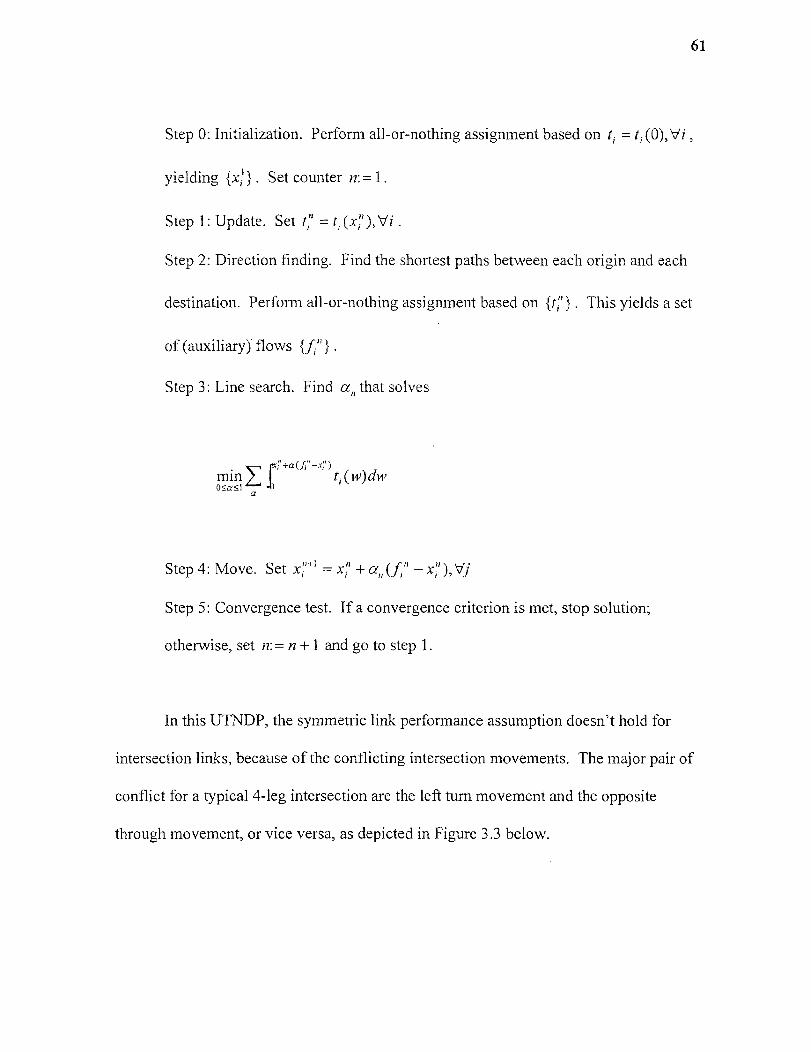
61
Step 0: Initialization. Perform all-or-nothing assignment based on t, = t,(0),Vi ,
yielding {4}. Set counter n:=1.
Step 1: Update. Set 1," =
Step 2: Direction finding. Find the shortest paths between each origin and each
destination. Perform all-or-nothing assignment based on {ti"} . This yields a set
of (auxiliary) flows {f,"}.
Step 3: Line search. Find a„ that solves
min in+a(fni-xni)ti (w)dwa
Step 4: Move. Set x:`+' = x , + a„(fi," — xni),Vj
Step 5: Convergence test. If a convergence criterion is met, stop solution;
otherwise, set n:= n + 1 and go to step 1.
In this UTNDP, the symmetric link performance assumption doesn't hold for
intersection links, because of the conflicting intersection movements. The major pair of
conflict for a typical 4-leg intersection are the left turn movement and the opposite
through movement, or vice versa, as depicted in Figure 3.3 below.
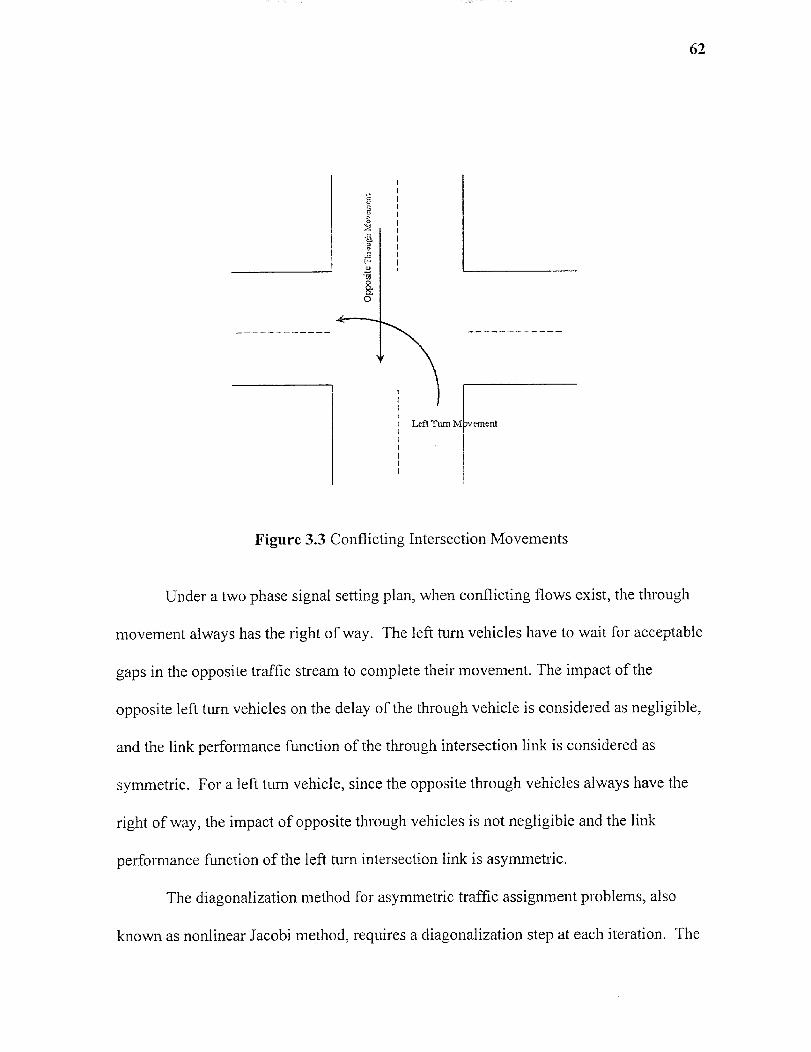
Left Turn M Movement
Figure 3.3 Conflicting Intersection Movements
Under a two phase signal setting plan, when conflicting flows exist, the through
movement always has the right of way. The left turn vehicles have to wait for acceptable
gaps in the opposite traffic stream to complete their movement. The impact of the
opposite left turn vehicles on the delay of the through vehicle is considered as negligible,
and the link performance function of the through intersection link is considered as
symmetric. For a left turn vehicle, since the opposite through vehicles always have the
right of way, the impact of opposite through vehicles is not negligible and the link
performance function of the left turn intersection link is asymmetric.
The diagonalization method for asymmetric traffic assignment problems, also
known as nonlinear Jacobi method, requires a diagonalization step at each iteration. The
62
63
diagonalizing step can be mathematically written as:
1"(x,) = Or in other words, 2'(X„) denotes the
performance function for links when all arguments of ta (-), other than x, , are fixed at
their values during the n th iteration. With all cross-link effects fixed, the performance
functions include only one argument, so at each iteration the problem is reduced to a
symmetric UE traffic assignment problem.
In the UTNDP, if link a is a left turn intersection link, then t a (x (.) =
where x„, is the opposite through flow. For all other types of links, the performance
functions are assumed symmetric and only include the subject link flows as independent
variables. The 1994 HCM intersection delay estimation procedure, which is used in this
UTNDP, does not consider cross-link effects. However, ta(ot,xa) can be estimated in
two steps. First, calculate t„ (x,), and then t„ (x,) is approximated to a value close to
ta(xa) = ta(xotxa) by dividing with a weight factor a1 that is also known as the left
turn adjustment factor. The left turn adjustment factor reflects the impact of the opposite
through movement on the subject left turn movement by dividing the green of the subject
lane group into several critical periods. At each symmetric iteration in the
diagonalization step, a estimated from the flows of the previous solution state, and
thus reflects the diagonalization nature of the procedure.
3.2.5 Lane Group Designation Procedure
The lane group designation procedure is important to the estimation of link performance
functions, because intersection delays are calculated by lane group. Therefore, before the
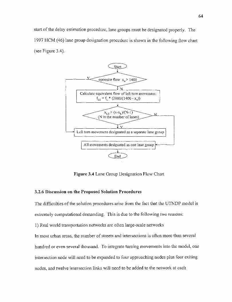
XLE (X-X L)/(N- )(N is the number of lanes
Calculate equivalent flow of left turn movement:
fLE =L * (2000/(1400 - x 0))
Left turn movement designated as a separate lane group
All movements designated as one lane group
start of the delay estimation procedure, lane groups must be designated properly. The
1997 HCM (46) lane group designation procedure is shown in the following flow chart
(see Figure 3.4).
Start
End
Figure 3.4 Lane Group Designation Flow Chart
3.2.6 Discussion on the Proposed Solution Procedures
The difficulties of the solution procedures arise from the fact that the UTNDP model is
extremely computational demanding. This is due to the following two reasons:
1) Real world transportation networks are often large-scale networks
In most urban areas, the number of streets and intersections is often more than several
hundred or even several thousand. To integrate turning movements into the model, one
intersection node will need to be expanded to four approaching nodes plus four exiting
nodes, and twelve intersection links will need to be added to the network at each
64
65
intersection. Therefore, the original network will be expanded to a size much larger than
the original network that is already very large.
2) The tri-level iterations involved in the model
There is a tri-level iteration involved in the solution algorithm of the model: (1) Solution
to the lower level problem. Given a network configuration and the O-D matrix, the
asymmetric traffic assignment is solved, (2) Solution to the upper level problem. Given
the new traffic flow pattern, a new network configuration is proposed by conducting a
heuristic search step, (3) Signal timing optimization. A new signal timing is found based
on the network configuration and the new traffic flow pattern.
At the lower level, the diagonalization step has to be performed at each
diagonalization iteration, and the shortest path subroutine has to be called repeatedly. At
the upper level iteration, given a large size network, the number of upper level decision
variables y is very large. The heuristic search procedure is computationally expensive
due to the large number of decision variables y. The third level of the iteration involved
here is the signal timing optimization procedure. Every time the network configuration
or flow pattern changes, the signal timing will need to be changed, so the signal timing
optimization procedure that is a large-scale nonlinear programming subroutine will be
called repeatedly.
The procedure can be expanded to include up to eight phases. In a real world
implementation of the UTNDP, this will be desirable, however this will further
exacerbate the computational performance of the procedure.
There is a need to develop a more comprehensive travel time function that
includes offsets as a variable. A consolidation between Gartner's delay formula and the
1994 HCM delay formula is necessary, in order to have more consistency between the
traffic assignment and the signal timing optimization steps.
The cycle length in most urban signalized networks has the same value at all
intersections. This approach is used also within the UTNDP. It is noted, however, that
this approach constraints the problem to a potential "sub-optimal" solution. A more
comprehensive approach would have been to use the cycle length as a variable for each
iteration.
66

CHAPTER 4
IMPLEMENTATION OF THE UTNDP SOLUTION HEURISTICS
This chapter presents the computer program implementation of the UTNDP solution
algorithm. Programs are coded in FORTRAN 77, and complied by Fortran PowerStation
4.0 on a PC with Pentium 11350 processor and 64MB memory.
4.1 Overview
The structure of the UTNDP programs is presented in Figure 4.1. There are 34
subroutines in the UTNDP programs, and the three major subroutines are `UPDATE_Y',
`SIGNALSET' and `DIAGONALIZATION'. Subroutine 'UPDATE_Y' is designed to
update the upper level network configuration variables; `SIGNALSET' is the upper level
signal setting optimization subroutine; `DIAGONALIZATION' is used to solve the lower
level asymmetric traffic assignment problem. Subroutines `UPDATE_Y' calls the
'UPDATE HEF' and the 'UPDATE HISCON' subroutines to implement the proposed
SA-TABU search strategy. Subroutine `SIGNALSET' calls a nonlinear programming
routine 'NONLINEAR' that is composed of a set of programs developed by Dow (53)
(these subroutines are not included in the 34 programs coded by the author of this
dissertation). These non-linear optimization programs were originally developed as an
independent package, however, several modifications were made to some of the
programs so that they could be embedded in the UTNDP program. Among these
modified programs, '1377', the input and nonlinear model construction file, has been
significantly changed to fit the requirements of other routines of the UTNDP program.
Subroutine `DIAGONALIZATION' calls 'LIE' repeatedly to solve a series of symmetric
67

68
traffic assignment problems. Two important routines that work together with UE are
`DELUPDATE' and 'DIAGDEL'. The first routine is used to update realistic link
performance functions, while the second one is used to calculate the impact of conflicting
opposite through movement on the delay of the subject left turning movement. Other
major UTNDP subroutines include link-locating routines ('OPPOLINK, 'ADJLINKR'
and ‘CONFLICTLINK'), and data format conversion routines ('FUETOSIG' and
`FSIGTOUE'), which are used to connect major UTNDP components by converting the
data format to a compatible form so that all programs can work together. Subroutine
'conmin' calls a set of programs developed by Dow (53); these programs are not included
in Figure 4.1.
4.2 The UTNDP Main Program
The main UTNDP program follows the steps presented in section 3.2.1. These steps are:
initialization, update upper level decision variable y, update saturation flow rates, solve
signal setting, solve the lower level asymmetric UE traffic assignment, update historical
contribution values, and heuristic search termination test. The UTNDP main program is
presented in Figure 4.4.
There are two types of solution states in the UTNDP SA-TABU heuristic, the
current state and the trial state. The current state is the accepted state with the accepted
link flows, signal settings, and network configuration parameters. Trial states are
generated based on the current state by perturbing network configuration variable y.
Any changes in y lead to changes in the signal settings and link flows. The acceptance
criteria in the heuristic search procedure of the UTNDP model are used to decide if a trial
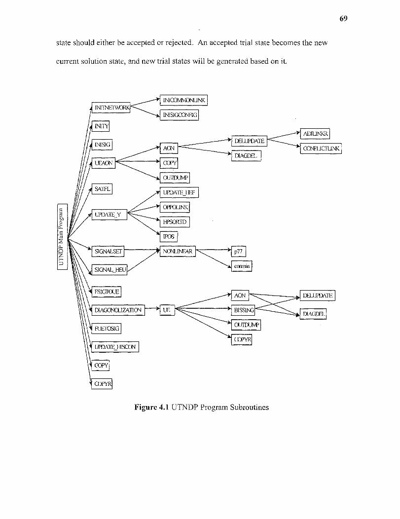
tat)0
state should either be accepted or rejected. An accepted trial state becomes the new
current solution state, and new trial states will be generated based on it.
69
Figure 4.1 UTNDP Program Subroutines
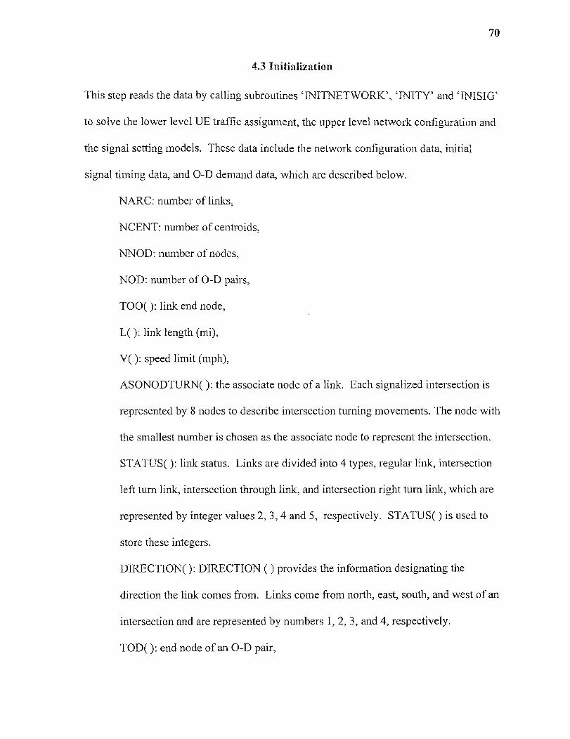
70
4.3 Initialization
This step reads the data by calling subroutines 'INITNETWORK, 'INITY' and INISIG'
to solve the lower level UE traffic assignment, the upper level network configuration and
the signal setting models. These data include the network configuration data, initial
signal timing data, and O-D demand data, which are described below.
NARC: number of links,
NCENT: number of centroids,
NNOD: number of nodes,
NOD: number of O-D pairs,
TOO( ): link end node,
L( ): link length (mi),
V( ): speed limit (mph),
ASONODTURN( ): the associate node of a link. Each signalized intersection is
represented by 8 nodes to describe intersection turning movements. The node with
the smallest number is chosen as the associate node to represent the intersection.
STATUS( ): link status. Links are divided into 4 types, regular link, intersection
left turn link, intersection through link, and intersection right turn link, which are
represented by integer values 2, 3, 4 and 5, respectively. STATUS( ) is used to
store these integers.
DIRECTION( ): DIRECTION ( ) provides the information designating the
direction the link comes from. Links come from north, east, south, and west of an
intersection and are represented by numbers 1, 2, 3, and 4, respectively.
TOD( ): end node of an O-D pair,
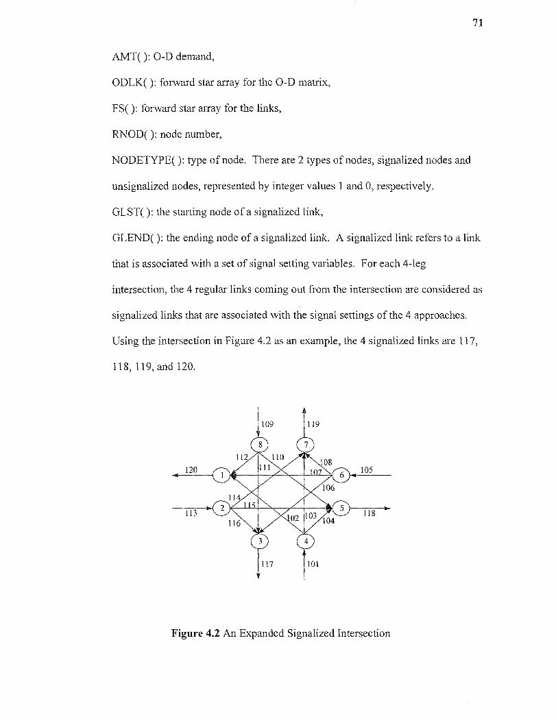
71
AMT( ): O-D demand,
ODLK( ): forward star array for the O-D matrix,
FS( ): forward star array for the links,
RNOD( ): node number,
NODETYPE( ): type of node. There are 2 types of nodes, signalized nodes and
unsignalized nodes, represented by integer values 1 and 0, respectively.
GLST( ): the starting node of a signalized link,
GLEND( ): the ending node of a signalized link. A signalized link refers to a link
that is associated with a set of signal setting variables. For each 4-leg
intersection, the 4 regular links coming out from the intersection are considered as
signalized links that are associated with the signal settings of the 4 approaches.
Using the intersection in Figure 4.2 as an example, the 4 signalized links are 117,
118, 119, and 120.
Figure 4.2 An Expanded Signalized Intersection
72
The ASONODTURN, STATUS, and DIRECTION arrays represent the
configuration of the network. Figure 4.2 presents a typical expanded signalized
intersection.
Nodes 1 to 8 represent an expanded signalized intersection. Links 101 to 120
represent all the links associated with the intersection. The ASONODTURN, STATUS,
and DIRECTION values of the links are described in Table 4.1.
Table 4.1 Link Configuration Values of a Sample Intersection
Link Number (1) ASONODTURN(I) STATUS(I) DIRECTION(I)101 1 2 3102 1 3 3103 1 4 3104 1 5 3105 1 2 2106 1 3 2107 1 4 2108 1 5 2109 1 2 1110 1 3 1111 1 4 1112 1 5 1113 1 2 4114 1 3 4115 1 4 4116 1 5 4117 1 2 3118 1 2 4119 1 2 2120 1 2
Saturation flow rates and link flows are also initialized in this step, using
subroutines SATFL' and ‘UEAON', respectively. Subroutine ‘SATFL' will be
presented in section 4.5. The heuristic search related parameters, the initial temperature,
initial Markov chain length, temperature dropping rate, Markov chain length increasing
rate, TABU list length, and the weights of the 3 components of the HEF, are also
initialized in this step.

73
4.4 Update Upper Level Decision Variable y
At each UTNDP iteration, the upper level decision variable y (lane designation and
intersection movement control variables) are updated based on the HEF values and the
TABU status of each link. The HEF has three components, the link v/c ratio, the
historical contribution, and the random factors. The link v/c ratio reflects the current
traffic performance on the subject link. Since the objective of the UTNDP is to minimize
network-wide link travel time, the larger the heuristic value is, the better the chance that
the subject link is chosen to be updated. This is because links with high v/c ratios often
experience much larger delays than links with low v/c ratios. For the two types of
updateable links, the calculation of v/c ratio for regular links is straightforward, while the
calculation of the v/c ratio for left turn intersection links requires lane group status
information. If the subject left turn, the corresponding through and right turn intersection
links are in one lane group, the v/c ratio of this whole lane group is calculated and
assigned to the left turn link. If the subject left turn intersection link is in a separate lane
group, its v/c ratio is calculated separately. The difference between the network UE total
travel time of the trial state and the current state is calculated, stored and accumulated as
the historical contribution of the trial state y value of the updated link. If the network-
wide UE total travel time of the trial state is less than that of the current state, then a
negative historical contribution of the trial y value is recorded. The smaller the
historical contribution value is, the less chance the subject link has to be chosen as the
candidate link to be updated. If the trial state solution is better than the current best
solution, the trial y value is rewarded by multiplying the historical contribution by a
credit factor larger than 1.
74
Subroutine 'UPDATE Y' is used to update the upper level decision variable y.
The input of subroutine 'UPDATE_Y' is YIN ( ), the output is YOUT( ), representing the
updated YIN ( ). The link with the highest HEF value among all the links not in the
TABU lists is selected to be updated, because high HEF values represent inappropriate
traffic performance on the link. Subroutine 'UPDATE_Y' starts with calling a
subroutine 'UPDATE HEF' to update HEF values. Then subroutine 'HPSORTD' is
called to sort the HEF values in descending order, where the sorted HEF values are stored
in array HEFORD( ). Another subroutine 'IPOS' is called to match elements in
HEFORD( ) with their original index in HEF( ), and the matched indexes are stored in
IPOS1( ). The current TABU status TABUSTATUS( I) stores the most recent iteration
number under which link I is updated. The difference between the current iteration
number ITE and TABUSTATUS(I) represents the number of iterations in which link I
hasn't been changed. If this difference is greater than a preset TABU length value, then
link I is updateable. Otherwise, the TABU status prevents link I from being updated. If
the selected link is a regular link, an additional lane is added to the link to alleviate the
condition of the link, and one lane has to be reduced from the opposite link. Update the
temporary TABU status TEMPSTATUS( for both the subject link and its opposite link
to ITE. If the selected link is a left turn link, and it is in a separate lane group, then
update YIN(IPOS1(I)) from 1 to 0, and set the TEMPSTATUS( ) of the selected left turn
link to ITE. If the selected link is a left turn link and it is in the same lane group with the
through and right turn links, then update YIN(IPOSI(I)) from its current state (0 or 1) to
a new state (1 or 0), set TEMPSTATUS( ) of the selected left turn link to ITE. When the
left turn link is in the same lane group with the through and the right turn links, its HEF
75
value is composed of the historical contribution factor, the random factor, and the v/c
ratio of the whole lane group rather than those of the left turn link itself. The flow chart
of subroutine 'UPDATE Y' is presented in Figure 4.6. Every time y is updated, a trial
state is created. Under the trial state, signal setting and traffic assignment subroutines are
performed, and the results are checked to decide if the trial state is accepted as the current
state. If the trial state is accepted, TEMPSTATUS( ) is copied to TABUSTATUS( ).
4.5 Update Saturation Flow Rates
Based on link flows, network confrguration, and lane group designations, the saturation
flow rates that will be used to construct both the objective function and the capacity
constraints in the signal setting model need to be updated prior to the signal setting and
the UE traffic assignment steps.
Subroutine `SATFL' starts with checking the status of the subject link. If link I is
a regular link, the saturation flow rate is calculated as:
STF(I)=Y(I) x1900 x a, x am, x ag x a, x a a„.
The number of lanes of this regular link is represented by Y(I) , while all the other
parameters are the same as described in equation (3.28). If link I is a through or a right
turn link, STF(I) is temporarily set to 9999, which is updated after the corresponding left
turn intersection link is checked. If link I is a left turn intersection link, it could be
designated as a separate left turn lane group, or the left turn, through, and the right turn
links are designated as one lane group. The lane group designation not only depends on
76
the flows of these links themselves, but also on the traffic flow of the opposite through
link, which is called the conflicting flow. Subroutines CONFLICTLINK' and
'ADJLINKR' are called to find the conflicting link and the approaching regular-in link.
If the regular-in link only has one lane, all movements are designated as one lane group,
otherwise, check opposite through link flow f0 to decide the appropriate lane group
designation. If fo is greater than 1400, link I is treated as a separate left turn lane group,
STF(I) 1900 x y, y is a constant which varies with fo . The saturation flow rate of the
other lane group (composed of through and right turn movements) is estimated as:
STF(I)= (Y(k)-1) x1900 x xaHV xagxapxabbxaaxaRT
k is the approaching regular-in link. In the UTNDP model, left, through and right turn
movements are ordered as I, I+1, and 1+2. Since through and right turns are always in
one lane group, STF(I+2) need not be estimated in this subroutine. If L is less than
1400, FLLE(I) (the left turn volume equivalent) and AVGFL (the average volume of the
through and the right turn lane group) are calculated. If FLLE(I) is less than or equal to
AVGFL, then the left turn link I is in a separate lane group, and STF(I) and STF(I+1) are
estimated the same way as described before. If FLLE(I) is greater than AFGFL, all
movements are designated as one lane group, and the saturation flow rate is calculated as:
STFI +1) = Y(k)x1900x aHV. RT xaLTg L f •

77
To estimate a LT , calculate gf (average amount of green time before the an .ival of
the first left turn vehicle), g„ (the average amount of green time after the arrival of the
first left turn), and Pi, (the proportion of left turn vehicle in the left lane), using the
methods proposed in section 3.2.3. The flow chart of subroutine `SATFL: is presented in
Figure 4.6.
4.6 Solve Signal Setting
In each UTNDP iteration, signal settings are set by calling subroutine 'SIGNALSET'. All
other offsets other than the ones directly optimized by the signal setting model can be
calculated by calling subroutine `OTHEROFFSET.
Subroutine `SIGNALSET' is used to obtain optimal green splits and offsets. The
green splits and offsets for a typical 4-leg intersection are presented in Figure 4.3:
Intersection I
Intersection 2
G 3
G14
OFFSET,,
Figure 4.3 Signal Setting Variables
78
G 1 2, G13 and G14 represent the effective green times allocated to the 4 approaches of
intersection 1. Variable Q12 represents the offset between intersection 1 and 2. The
following equations have to be satisfied:
= G 13
G 1 , = G 14
G 1G, 2 = cycle length (Or. G 13 + G 14 = cycle length)
Given any of the 4 green splits, the others can be derived from the above
equations. So, for each intersection, only one green split variable, namely G 11 , is used in
the signal setting model as a decision variable. All the other green splits are represented
as a function of G 11 , and their contributions to the objective function are also represented
by G11. By doing so, both the number of decision variables and the number of
constraints can be reduced significantly in the signal setting model. To obtain reasonably
good signal setting results, the UTNDP is solved 12 times using fixed cycle length
ranging from 60 to 120 seconds with 5 second increments, and then the result with the
smallest network wide total travel time is selected as the solution of the signal setting
model.
Given link flows and the network configuration variable y, subroutine
`SIGNALSET' must be solved before proceeding to the lower level UE traffic
assignment step. However, there is the possibility that subroutine `SIGNALSET' doesn't
have a solution. If this happens, the program goes back to subroutine 'UPDATE Y' to
choose another y to be updated. If after a number of trials, the 'SIGNALSET'
79
subroutine is still not solvable, then reinitialize the green splits, offsets, and the cycle
length, and proceed to the asymmetric traffic assignment subroutine
'DIAGONALIZATION'. The search is then directed to a new search area, starting with
initial signal settings and current link flows. The flowchart of this process is presented in
Figure 4.7.
The data format of the link flows and saturation flows, which are obtained from
the `DIAGONALIZATION' subroutine and used as input to subroutine `SIGNALSET',
is not compatible with the requirements of subroutine 'SIGNALSET'. Similarly, the
signal setting results, which are obtained from 'SIGNALSET' and used as input to
subroutine `DIAGONALIZATION' are not compatible with the requirements of
‘DIAGONALIZATION' either. Before calling `SIGNALSET', subroutine `FUETOSIG'
is called to convert link flows and saturation flows to a format compatible with
`SIGANLSET'. After `SIGNALSET', subroutine TSIGTOUE' is called to convert
signal setting results to a format compatible with `DIAGONALIZATION'.
4.7 Solve the Lower Level Asymmetric UE Traffic Assignment
The existence of the asymmetric impact of the opposite through vehicles on the left turn
vehicles requires a diagonalization procedure to solve the lower level UE traffic
assignment. The diagonalization is achieved by approximating the asymmetric problem
with a series of symmetric problems. Symmetric problems are solved using the Frank-
Wolfe algorithm.
One of the major differences between this study and previous traffic assignment
studies is that a more realistic link performance function is used rather than the BPR

80
curve. The performance function is described in section 3.1.2. The independent
variables of the performance function not only include link flows, but also signal timings
and saturation flow rates. Subroutine 'DELUPDATE' is used to update the link
performance function in this study.
The diagonalization of an asymmetric traffic assignment problem requires a link
performance function that includes both the subject link flow and the conflicting flows as
independent variables. So far, no such functions have been proposed. In this study, a left
turn adjustment factor is used to account for the impact of the conflicting opposite
through movement on the left turn movement delays. Subroutine `DIAGDEL' is
designed for this purpose. Subroutines `DELUPDATE' and `DIAGDEL' are discussed
in the next paragraph.
In subroutine ‘DELUPDATE', if the subject link I is a regular link, the delay on
the link DL(I) is estimated using equations (3.21) and (3.22). If link I is a left turn link
and it is in a separate lane group, calculate uniform delay DU(I) and random delay DA(I)
using equations (3.14) and (3.15), respectively. The link flows, saturation flows and
signal timings on link I are obtained and used as inputs to subroutine `DELUPDATE'.
The corresponding through and right turn delay DL(I+1) and DL(I+2) are calculated in
the same way. If link I is a left turn link and left, though and right turn movements are in
one lane group, the delay on the approaching regular-in link DL(J) is calculated. Then
the delay on the subject left turn link DL(I) and the delays on the through and right turn
links DL(I+1) and DL(I+2) are derived from DL(J) ) using equation (3.24). In subroutine
`DELUPDATE', 'ADJLINKR' and `CONFLICTLINK' are called to find the

81
approaching regular-in link J and the conflicting opposite through link K. Subroutine
‘DELUPDATE ) is presented in Figure 4.8.
In subroutine DIAGDEL', if link I is a left turn link, calculate the average
amount of green time before the arrival of the first left turn vehicle GF(I), and the
average amount of green time required for the opposing standing queue to clear GQ(I),
using equations (3.34) and (3.35), respectively. Call subroutine `CONFLICTLINK' to
find the conflicting opposite through link K. If FLDG(K), the flow on link K from the
last iteration, is greater than 1400, then no left turn vehicle could be cleared at the
intersection, and the through car equivalent factor EL is assigned a very large value.
Otherwise, calculate EL as proposed in section 3.2.3. If GQ(I) is greater than GF(I), then
GU, the average amount of green time after the arrival of the first left turn vehicle that is
not blocked by the clearance of the opposing standing queue, equals to green G(I) minus
GQ(I). Otherwise, GU equals to G(I) minus GF(I). The proportion of left turn vehicles
in the left lane PL is calculated using equation (3.33). The left turn adjustment factor
FLL is calculated using equations (3.30)-(3.32). Finally, the delay estimated using the
subject link flow is converted to the delay that reflects the impact of the opposing through
movement by multiplying FLL. The flow chart of subroutine "DIAGDEL' is presented
in Figure 4.9.
4.8 Update Historical Contribution
The inclusion of the historical contribution factor in the HEF provides an additional
element in the search that rewards upper level decision variables y that performed well
in the previous iterations. By introducing the historical contribution factor, the search

82
becomes more informed and more focused on high quality feasible regions. Although
this may increase the risk of not finding the global optimal solution, it can increase the
efficiency of the search strategy significantly. Considering the computational complexity
of an UTNDP, it is necessary to find near optimal solutions within a reasonable number
of iterations. The inclusion of the historical contribution as one component of the HEF
may greatly reduce the number of iterations of finding a near optimal solution.
In each UTNDP iteration, historical contribution factors are only updated for the
links whose decision variable values are changed. Therefore, only left turn links and
regular links are associated with historical contribution values. There are two states of y
variables for left turn links, y either equals to 0 or equals to 1 (representing permission
and prohibition of the left turn movement, respectively). For regular link y variables, the
possible values are 1, 2 and 3, representing the number of lanes, respectively. For each
state of a y variable, there is an associated historical contribution value. The historical
contribution values of left turn links are stored in a 2-dimentional array HISCONI(i,j),
while the historical contribution values of regular links are stored in HISCONR(i,j).
Here, i represents the state of the y variable, and j represents the link number. The
historical contribution of a y state of a link is an accumulation of the performance index
of the state. The performance index used in this study is the difference between the
network-wide total travel times of the current state and the trial state. Each time the link
is updated, the difference is calculated and accumulated to the historical contribution
value. To better explain the mechanism of the process of calculating historical
contribution, two examples are given in the subsequent paragraphs. The first example is
designed for a left turn link, and the second one is designed for a regular link.
83
Example 1:
Given,
i: number of a left turn link updated in the trial state,
HISCONI(i,1): current historical contribution of state y(i)=0,
HISCONI(i,2): current historical contribution of state y(i)=1,
Current State: y(i)=0
Trial State: y(i)=1
Current State Network Total Travel Time: TRTIME C
Trial State Network Total Travel Time: TRTIME T
Current Contribution: RIMP=TRTIME C - TRTIME T
The historical contribution after the solution of the trial state is:
HISCONI(i,1)=HISCONI(i,1)+RIMP
HISCONI(i,2)=HISCONI(i,2)-RIMP
The contribution of y(i) changing from state 0 to state 1 is represented by RIMP.
If RIMP is negative, the solution of current state is better than that of trial state.
Therefore, HISCONI(i,l) is credited by reducing its value by the amount of RIMP, and
HISCONR(i,2) is penalized by increasing its value by the amount of -RIMP. If RIMP is
positive, the solution of the current state is worse than that of trial state. Therefore,
HISCONI(i,l) is penalized by increasing its value by the amount of RIMP, and
HISCONI(i,2) is credited by reducing its value by the amount of -RIMP. The y states of
links with small historical contribution values are considered as good candidates of
entering the final solution set, and they are less likely to be chosen as the links to be
updated.
84
Example 2:
Given,
i: number of a regular link updated in the trial state,
HISCONR(i,1): current historical contribution of state y(i)=1,
HISCONR(i,2): current historical contribution of state y(i)=2,
HISCONR(i,3): current historical contribution of state y(i)=3,
Current State: y(i)=2
Trial State: y(i)=3
Current State Network Total Travel Time: TRTIME C
Trial State Network Total Travel Time: TRTIME T
Current Contribution: RIMP=TRTIMEC - TRTIME T
The historical contribution after the solution of the trial state is:
HI SCONR(i, 1)=HISCONR(i, 1)
HISCONR(i,2)=HISCONR(i,2)+RIMP
HISCONR(i,3)=HISCONR(i,3)-RIMP
In example 2, y(i) is updated to y(i)=3, therefore, HISCONR(i,1), which represents the
state of y(i)=0, remains unchanged.
Subroutine 'UPDATE HISCON' is designed for the purpose of updating
historical contributions. If link I is a left turn link and the current state is Y(I)=0,
credit/penalize HISCON(I,l) by adding RIMP to its current value, while at the same time
penalize/credit HISCON(I,2) by subtracting RIMP from its current value. If link I is a
regular link and the current state is Y(I)=1, Y(I) can only be updated to Y(I)=2, therefore,
credit/penalize HISCONR(I,1) by adding RIMP, penalize/credit HISCONR(I,2) by

85
subtracting RIMP from its current value. If link I is a regular link and the current state is
Y(I)=3, Y(I) can only be updated to Y(I)=2, therefore, credit/penalize HISCONR(I,3) by
adding RIMP, and penalize/credit HISCONR(I,2) by subtracting RIMP from its current
value. If link I is a regular link, current state is Y(I)=2 and trial state YOUT(1)=1, then
credit/penalize HISCONR(I,2) by adding RIMP, penalize/credit HISCONR(I,l) by
reducing RIMP from its current value. If link I is a regular link, the current state is
Y(I)=2, and the trial state is YOUT(I)=3, then credit/penalize HISCONR(2,I) by adding
RIMP, penalize/credit HISCONR(I,3) by reducing RIMP from its current value.
Subroutine 'UPDATE HISCON' is presented in Figure 4.10.
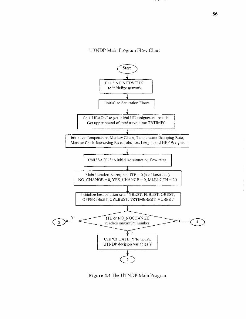
Initialize best solution sets: YBEST, FLBEST, GBEST,OFFSETBEST, CYLBEST, TRTIMEBEST, VCBEST
ITE or NO_NOCHANGEreaches maximum number
4,Call ‘UPDATE_Y'to updateUTNDP decision variables Y
4
Call `INITNETWORK'to initialize network
Initialize Temperature, Markov Chain, Temperature Dropping Rate,Markov Chain Increasing Rate, Tabu List Length, and HEF Weights
4,
Initialize Saturation Flows
Call `UEAON' to get initial UE assignment resutls;Get upper bound of total travel time TRTIMEO
4,
Call `SATFL' to initialize saturation flow rates
4,Main Iteration Starts; set: ITE = 0 (14 of iterations)
NO_CHANGE = 0, YES_CHANGE = 0, MLENGTH = 20
UTNDP Main Program Flow Chart
(tart)
4,
86
Figure 4.4 The UTNDP Main Program
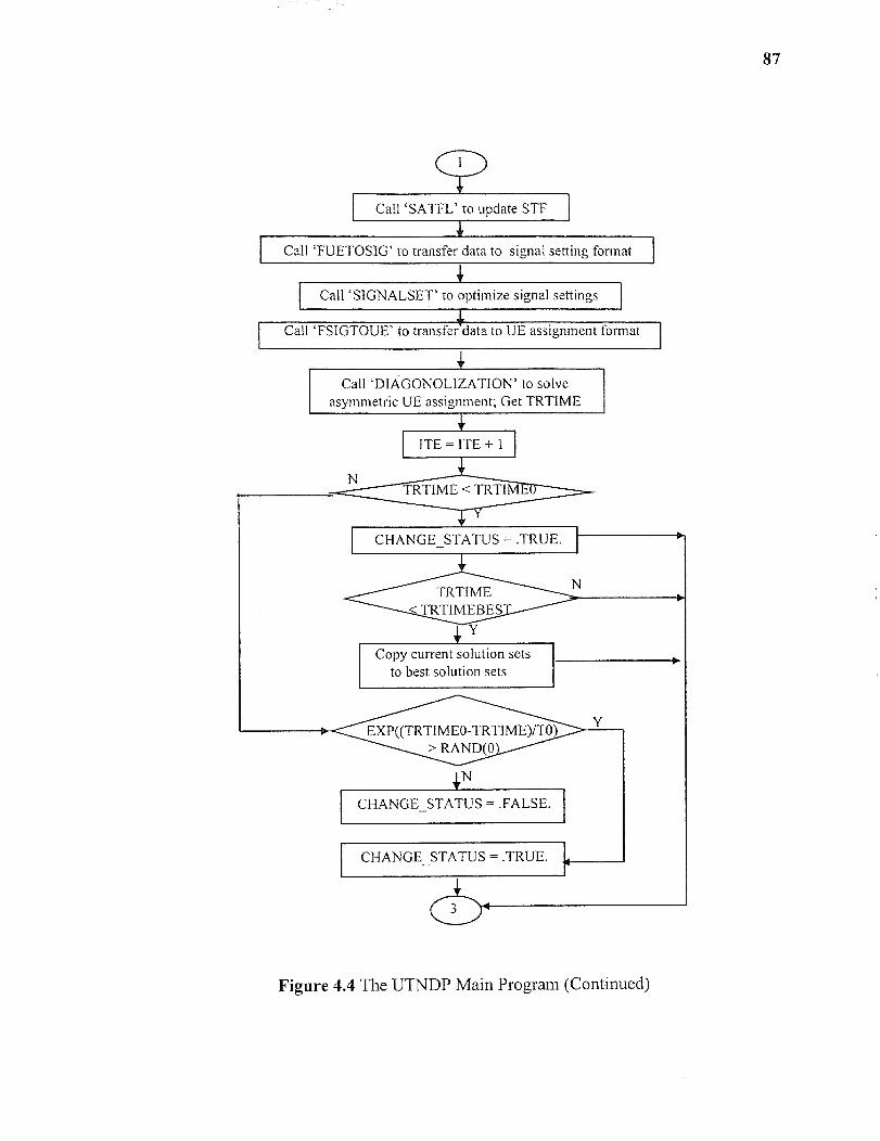
4ITE = ITE + I
Copy current solution setsto best solution sets
CHANGE STATUS = .TRUE.
EXP((TRTIMEO-TRTIME)/TO> RAND(0)
CHANGE_STATUS = .FALSE.
4Call `DIAGONOLIZATION' to solve
asymmetric UE assignment; Get TRTIME
Call TSIGTOUE' to transfer data to UE assignment format
4Call ‘SIGNALSET' to optimize signal settings
Call 'SATFL' to update STF
Call FUETOSIG' to transfer data to signal setting format
87
Figure 4.4 The UTNDP Main Program (Continued)
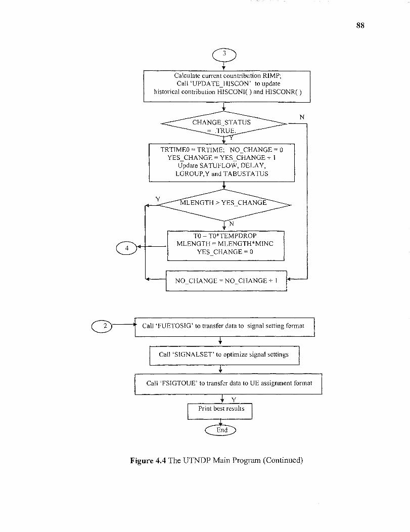
NCHANGE_STATUS
= .TRUE.
MLENGTH > YES_CHANGE
Calculate current countribution RIMP;Call `UPDATE_HISCON' to update
historical contribution HISCONI( ) and HISCONR( )
88
TRTIMEO = TRTIME„ NO_CHANGE = 0YES_CHANGE = YES_CHANGE + I
Update SATUFLOW, DELAY,LGROUP,Y and TABUSTATUS
4
TO = TO*TEMPDROPMLENGTH = MLENGTH*MINC
YES_CHANGE = 0
NO_CHANGE = NO_CHANGE + I
Call FUETOSIG' to transfer data to signal setting format
Call `SIGNALSET' to optimize signal settings
4Call FSIGTOUE' to transfer data to UE assignment format
YPrint best results
C—'L DEnd
Figure 4.4 The UTNDP Main Program (Continued)

I = NODEINDEX(J)
Calculate TABU length for each I:TABULENTGH( ) = ITE - TABUSTATUS( )
SUBROUTINE UPDATE_Y
(-Start
Call 'UPDATE_ HEF' to update HEF( )
Call HPSORTD to sort HEF( ) in descending order,output HEFORD( )
Call `IPOS' to match HEF( ) index with correspondingelements in HEFORD ( ), output IPOS I ( )
89
Figure 4.5 Subroutine UPDATE-Y
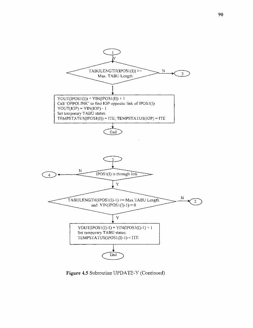
3
IPOS1(I) is through link
TABULENGTH(IPOS1(I)-1)>= Max.TABU Lengthand YIN(IPOS 1 (I)-I) = 0
N
YOUT(I POS I (I)-I) = YIN(IPOS1(I)-I) + ISet temporary TABU status:TEMPSTATUS(IPOS I (I)- 1 ) = ITE
C7)Y
TABULENGTH(IPOS I(I)) >=Max. TABU Length
< 2)
YOUT(IPOS 1 (I)) = Y 1N(IPOSI (I)) + ICall `OPPOLINK' to find I0P opposite link of IPOSI(I)YOUT(IOP) = YIN(I0P)- ISet temporary TABU status:TEMPSTATUS(IPOSI(I)) = ITE; TEMPSTATUS(IOP) = ITE
End
Figure 4.5 Subroutine UPDATE-Y (Continued)
90
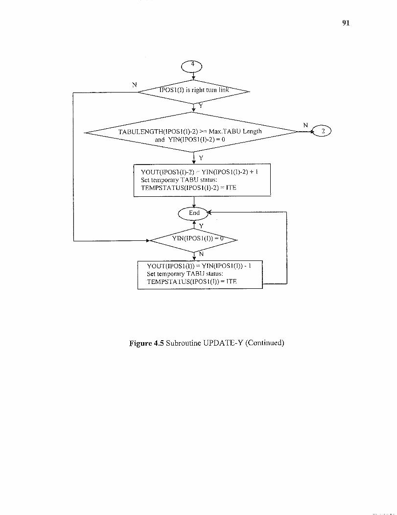
Y
N
( 4 )• POS I (I) is right turn lin
TABULENGTH(IPOS I (I)-2) >= Max.TABU Lengthand YIN(IPOS I (I)-2) = 0
YOUT(IPOSI(I)-2) = Y IN(IPOS 1 (I)-2) + ISet temporary TABU status:TEMPSTATUS(IPOS I (I)-2) = ITE
End
YOUT(IPOS I (I)) = Y IN(IPOS I (I)) - ISet temporary TABU status:TEMPSTATUS(IPOS I (I)) = 1TE
Figure 4.5 Subroutine UPDATE-Y (Continued)
91
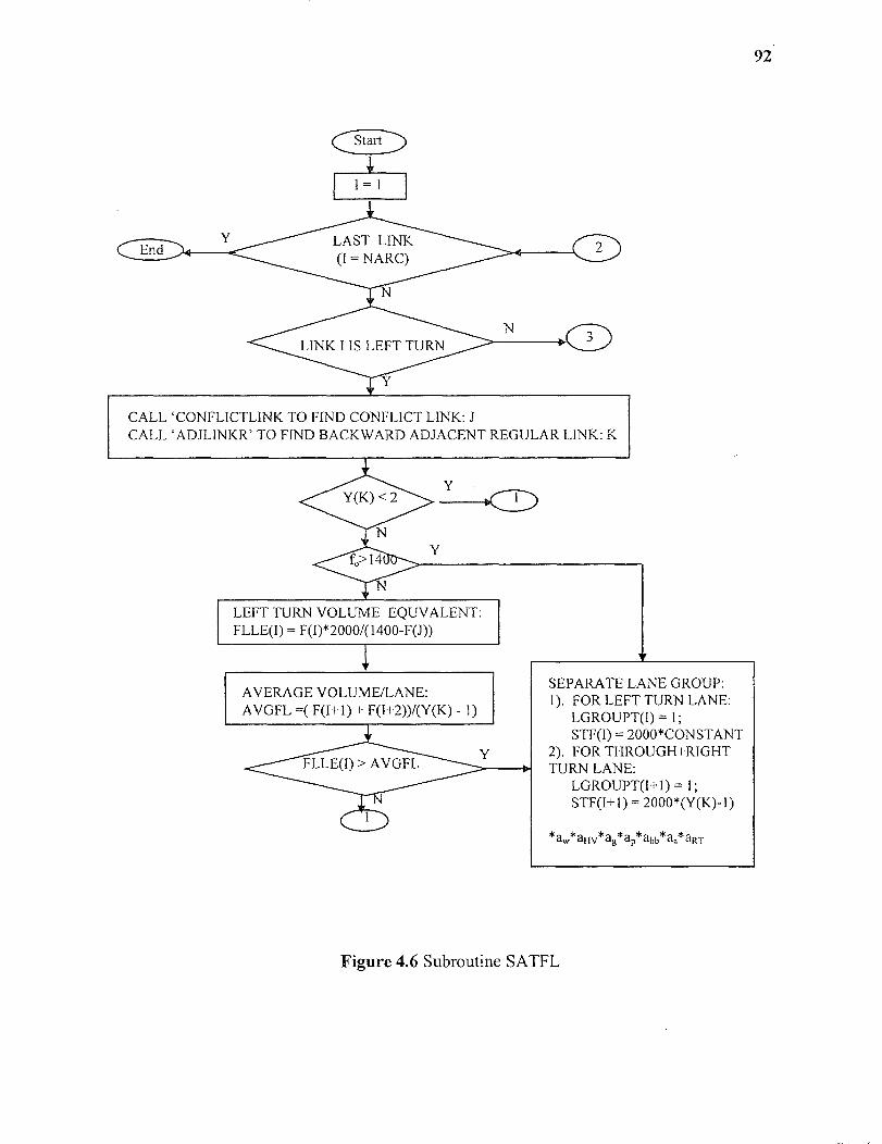
CALL `CONFLICTLINK TO FIND CONFLICT LINK: JCALL 'ADJLINKR' TO FIND BACKWARD ADJACENT REGULAR LINK: K
Start
92
LEFT TURN VOLUME EQUVALENT:FLLE(I) = F(I)*2000/(1400-F(J))
AVERAGE VOLUME/LANE:AVGFL =( F(I+1) + F(I+2))/(Y(K) - 1
SEPARATE LANE GROUP:1). FOR LEFT TURN LANE:
LGROUPT(I) = I;STEW = 2000*CONSTANT
2). FOR THROUGH+RIGHTTURN LANE:
LGROUPT(I+1) = I;STF(I+1) = 2000*(Y(K)-1)
*aw*aHV*ag*ap*abb*aa*A=artp a bb a a
Figure 4.6 Subroutine SATFL
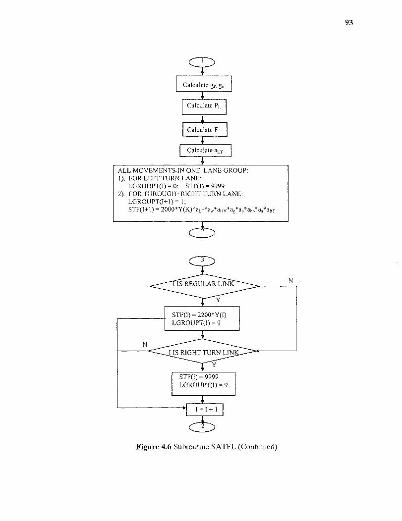
Calculate g f, gu
Calculate P L
ALL MOVEMENTS IN ONE LANE GROUP:I). FOR LEFT TURN LANE:
LGROUPT(I) = 0; STF(I) = 99992)LT FOR THROUGH+RIGHT TURN LANE:
LGROUPT(I+I)= I;STF(I+I) = 2000*Y(K)*aLT* HV*ag*ap*abb*aa*aRT
93
STF(I) = 2200*Y(I)LGROUPT(I) =9
STF(I) = 9999LGROUPT(I) =9
Figure 4.6 Subroutine SATFL (Continued)

Call 'UPDATE_Y' to get new network configurations
Put newly updated y to SIGSETTABU( )
Link Flows FromAsymmetric
Call 'SATFL' to update saturation flow rates
YITE = Max. iteration No.
Call `FUETOSIG'
Call `SIGNALSET' to solve signal setting
NOUNSUCC = NOUNSUCC +
Reinitialize signal
Call ‘FSIGTOUE'
Call `DIAGONAL ZATION' to solve asymmetric traffic assignment
TE = ITE +
94
End
Figure 4.7 Iterations of Signal Setting in UTNDP Main Program
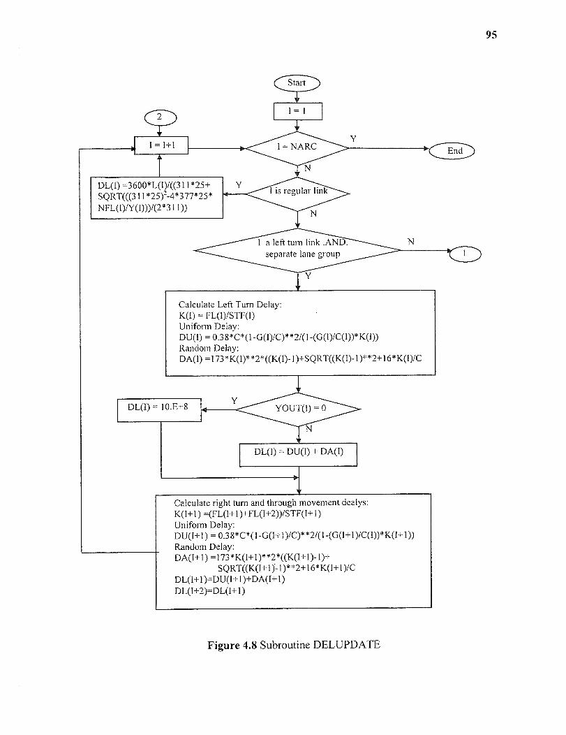
I = I+1
DL(I) =3600*L(I)/((311*25+SQRT(((311*25)2-4*377*25*
NFL(I)/Y(I)))/(2*311))
95
Start
4. 1=
I a left turn link .AND. Nseparate lane group
Calculate Left Turn Delay:K(I) = FL(I)/STF(I)Uniform Delay:DU(I) = 0.38*C*(1-G(I)/C)**2/(1-(G(I)/C(I))*K(I))Random Delay:DA(I) =173*K(I)**2*((K(I)-I)+SQRT((K(I)-I)**2+16*K(I)/C
DL(I) = 10.E+8
DL(I) = DU(I) + DA(I)
Calculate right turn and through movement dea ys:K(I+I) =(FL(I+I)+FL(I+2))/STF(I+1)Uniform Delay:
DU(I+1) = 0.38*C*(I-G(I+I)/C)**2/(I2(G(I+I)/C(I))*K(I+1))Random Delay:
DA(I+1) =173*K(I+1)**2*((K(I+1)-1)+SQRT((K(I+1)-1)**2+16*K(I+1)/C
DL(I+1)=DU(I+1)+DA(I+1)DL(I+2)=DL(I+1)
Figure 4.8 Subroutine DELUPDATE
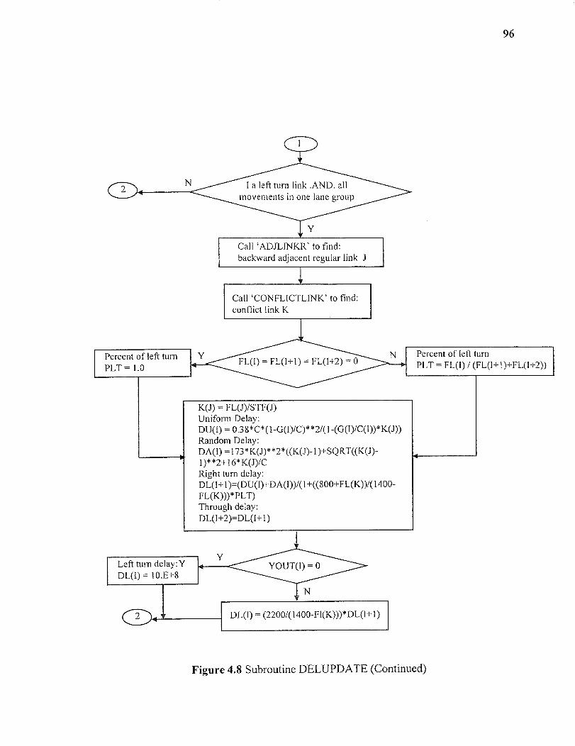
I a left turn link .ANDLT allmovements in one lane group
FL(I) = FL(I+l) = FL(I+2) = 0
Call `ADJLINKR' to find:backward adjacent regular link J
Call `CONFLICTLINK' to find:conflict link K
1
96
Percent of left turnPLT = FL(l) / (FL(l+1)+FL(l+2))
Percent of left turnPLT = 10
K(J) = FL(J)/STF(J)Uniform Delay:
DU(I) = 0.38*C*(I-G(I)/C)**2/ 1-(G(I)/C(I))*K(J))Random Delay:DAM =173*K(J)**2*((K(J)-I)+SQRTRK(J)-I)**2+16*K(J)/CRight turn delay:DL(I+I)=(DU(I)+DA(1))/(I+((800+FL(K))/(1400-FL(K)))* PLT)Through delay:
DL(I+2)=DL(I+1)
Left turn delay:YDL(I) = 10.E+8
DL(I) = (2200/(1400-Fl(K)))*DL(I+I)
Figure 4.8 Subroutine DELUPDATE (Continued)
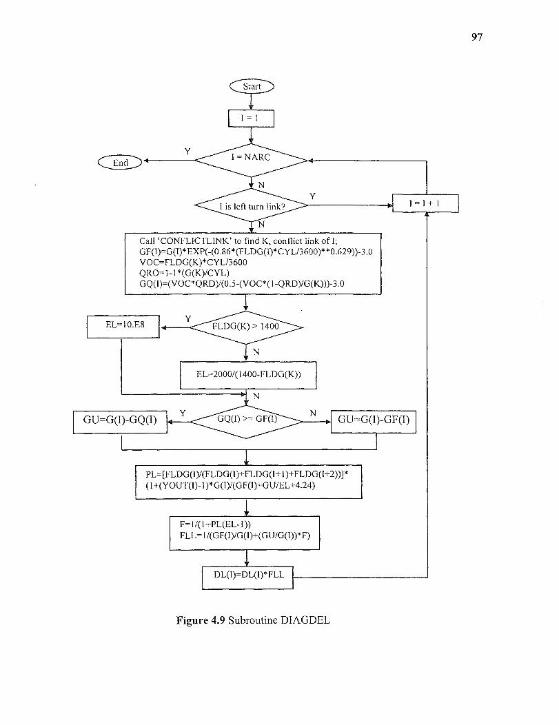
Call 'CONFLICTLINK' to find K, conflict link of 1;GF(I)=G(I)*EXP(-(0.86*(FLDG(I)*CYL/3600)**0.629))-3.0VOC=FLDG(K)*CYL/3600QRO=I-I*(G(K)/CYL)GQ(I)=(VOC*QRD)/(0.5-(VOC*(I-QRD)/G(K)))-3.0
GU=G(I)-GQ(I)
EL=10.E8
EL=2000/(14002FLDG(K))
GQ(I) >= GF(I) GU=G( )-GF(I)
FLDG(K) > 1400
F=I/(I+PL(EL- I ))FLL=I/(GF(I)/G(I)+(GU/G(I))*F)
Figure 4.9 Subroutine DIAGDEL
DL( =DL(I)*FLL
97
PLIFLDG(I)/(FLDG(I)+FLDG(I+1)+FLDG(I+2))]*(I+(YOUT(I)-1)*G(I)/(GF(I)+GU/EL+4.24)

Y N
I is a left turn link?
HISCONI(I,1) = H SCONI(I,1) + RIMPHISCONI(I,2) = HISCONI(I,2) - RIMP
HISCONI(I,2)= H SCONI(I,2) + RIMPHISCONI(I,1) = H SCONI(I,1) - RIMP
is a regular
HISCONR(I,1) = HISCONR(I,1)+ RIMPHISCONR(I,2) = HISCONR(I,2) - RIMP
N
HISCONR(3,I) = HISCONR(3,I) + RIMPHISCONR(2,I) = HISCONR(2,I)- RIMP
OUT(I) =
HISCONR(2,I) = HISCONR(2,I) + RIMPHISCONR(3,I) = HISCONR(3,I)- RIMP
H SCONR(2,I)= HISCONR(2,I) + JUMPHISCONR(I,I) = HISCONR(1,I) - RIMP
END
98
Figure 4.10 Subroutine UPDATE-HISCON
CHAPTER 5
NUMERICAL EXPERIMENTS
This chapter presents numerical experiments of the SA-TABU based methodology to
solve the UTNDP outlined in Chapter 3. The primary objectives of these experiments are
to examine the characteristics of the solutions generated by this procedure. The
computational performance and the sensitivity on major algorithmic parameters of the
SA-TABU heuristic are presented in Chapter 6.
The SA-TABU search strategy used in this study is a heuristic that combines the
characteristics of simulated annealing and TABU search methods. Although the SA-
TABU heuristic can not guarantee an optimal solution, it is an efficient method that can
be used to locate reasonably good solutions within an acceptable amount of
computational time. To test the efficiency of the SA-TABU search procedure, the
numerical experiments need to cover as many networks with different configurations and
characteristics as possible. In this study, 4 small to medium sized networks are used for
experimental purposes, which are described in section 5.1, followed by the analysis of the
results.
5.1 Test Networks
Among the 4 test networks, 3 of them are grid networks, Network 1 (3 by 3), Network 2
(3 by 4), Network 4 (3 by 5), and the other one, Network 3, is an arterial. Network 4
includes 15 signalized intersections and can be used to represent a real urban network.
Therefore, Network 4 is used as the base-network of the traffic signal engineering
analysis of the solutions generated by the SA-TABU heuristic. The competition of
99
100
network resources, namely signal resources, between adjacent streets makes it very
difficult to achieve good traffic performance on all streets in a network. Priority is often
given to a major street or arterial that has heavy traffic. To study the performance of the
UTNDP model on an isolated street, an arterial with 6 signalized intersections is
included. The two smaller grid networks, together with the arterial, are used to conduct
the sensitivity analysis for the parameters of the SA-TABU search due to their relatively
small sizes. Turning movement control is one of the major concerns of this study. In
order to represent turning movements in a network, signalized intersections of test
networks need to be expanded using abstract intersection links as demonstrated in Figure
4.2. The structural and traffic characteristics of the four test networks are presented in the
subsequent sections.
5.1.1 Test Network Characteristics
Network 1: A graphical representation of network 1 is presented in Figure 5.1. Network
1 is a 3 by 3 grid network with 5 signalized intersections. This network has 4 centroids,
13 nodes and 32 links in the original network, and 56 nodes and 96 links in the expanded
network.
Network 2: A graphical representation of network 2 is presented in Figure 5.2.
Network 2 is a 3 by 4 grid network with 8 signalized intersections. This network has 6
outside centroids and 1 internal centroid, 19 nodes and 62 links in the original network,
and 94 nodes and 180 links in the expanded network.
Network 3: A graphical representation of network 3 is presented in Figure 5.3.
Network 3 is an arterial with 6 signalized intersections. This network has 14 centroids,
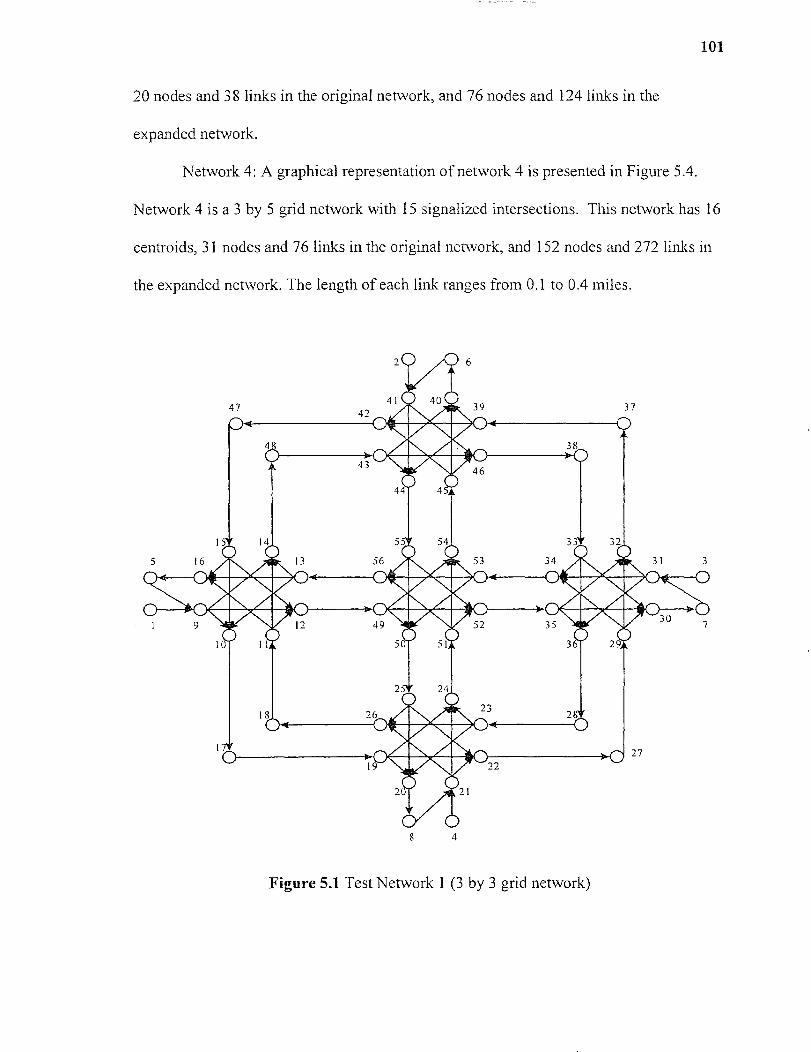
101
20 nodes and 38 links in the original network, and 76 nodes and 124 links in the
expanded network.
Network 4: A graphical representation of network 4 is presented in Figure 5.4.
Network 4 is a 3 by 5 grid network with 15 signalized intersections. This network has 16
centroids, 31 nodes and 76 links in the original network, and 152 nodes and 272 links in
the expanded network. The length of each link ranges from 0.1 to 0.4 miles.
4
Figure 5.1 Test Network 1 (3 by 3 grid network)
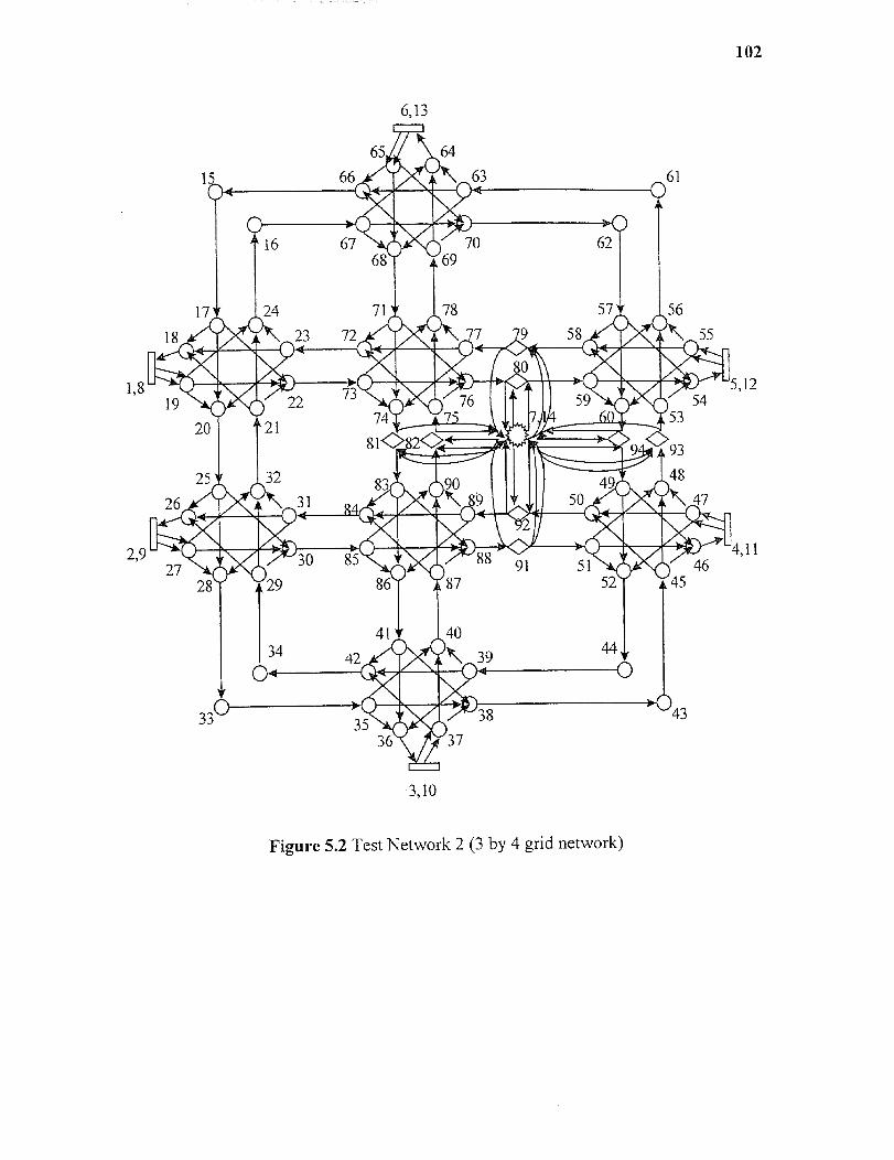
102
6,13
3,10
Figure 5.2 Test Network 2 (3 by 4 grid network)

I,15
103
2,16
3,17
4,18
14,28
13,27
12,26
53 • 060 5954• v.. •1*"AI Aftimi
'`V NIP 58
5655 • •
6 • 06862 4., .
6,20 114~21." Ai"
• 11
5,19
7,21 9,23
8,22
Figure 5.3 Test Network 3 (6-intersection arterial)
11,25
10,24

9,255,2
16,32 15,31 14,30
6,22 7,23 8,24
1, 17
2,18
3,19
4,20
3.29
12,28
11,27
0.26
1021011 12
111
Figure 5.4 Test Network 4 (3 by 5 grid network)
The Origin-Destination (O-D) matrices used in the analysis of the UTNDP for
each network are presented next.
104
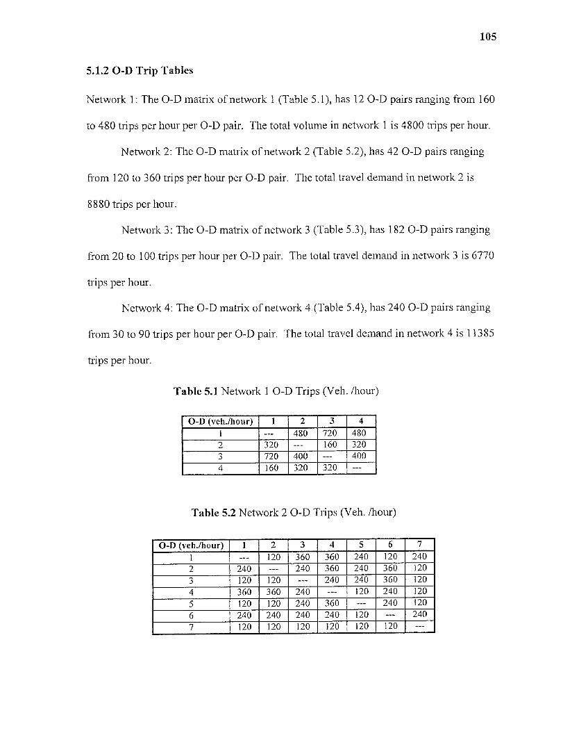
105
5.1.2 O-D Trip Tables
Network 1: The O-D matrix of network 1 (Table 5.1), has 12 O-D pairs ranging from 160
to 480 trips per hour per O-D pair. The total volume in network 1 is 4800 trips per hour.
Network 2: The O-D matrix of network 2 (Table 5.2), has 42 O-D pairs ranging
from 120 to 360 trips per hour per O-D pair. The total travel demand in network 2 is
8880 trips per hour.
Network 3: The O-D matrix of network 3 (Table 5.3), has 182 O-D pairs ranging
from 20 to 100 trips per hour per O-D pair. The total travel demand in network 3 is 6770
trips per hour.
Network 4: The O-D matrix of network 4 (Table 5.4), has 240 O-D pairs ranging
from 30 to 90 trips per hour per O-D pair. The total travel demand in network 4 is 11385
trips per hour.
Table 5.1 Network 1 O-D Trips (Veh. /hour)
O-D (veh./hour) 1 2 3 4
1 480 720 4802 320 --- 160 3203 720 400 4004 160 320 320 ---
Table 5.2 Network 2 O-D Trips (Veh. /hour)
0-D (veh./hour) 1 2 3 4 5 6 71 120 360 360 240 120 2402 240 240 360 240 360 1203 120 120 240 240 360 1204 360 360 240 --- 120 240 1205 120 120 240 360 --- 240 1206 240 240 240 240 120 2407 120 120 120 120 120 120 ---

106
Table 5.3 Network 3 O-D Trips (Veh. /hour)
O-D (veh./hour) 1 2 3 4 5 6 7 8 9 10 11 12 13 141 20 40 40 40 20 20 60 20 40 20 40 20 402 40 20 20 20 60 40 20 20 40 30 50 30 803 20 40 40 20 20 20 20 40 60 40 20 80 204 40 20 60 --- 40 40 40 20 60 40 60 60 40 205 40 20 40 60 --- 40 20 60 40 20 60 60 40 606 20 20 60 40 20 20 40 40 60 40 20 40 607 20 20 20 20 20 20 40 20 40 20 40 20 408 60 60 20 40 40 40 20 60 40 60 60 20 409 40 60 20 20 20 40 40 40 40 60 20 60 2010 40 60 40 60 20 20 40 20 40 60 40 40 2011 60 20 20 20 20 20 40 20 40 20 --- 40 20 4012 20 40 40 40 20 20 100 20 40 20 40 20 4013 60 40 40 60 20 60 60 40 40 60 40 60 4014 20 40 40 60 40 60 40 40 60 20 40 20 40
Table 5.4 Network 4 O-D Trips (Veh. /hour)
0-D(veh./hour)
1 2 3 4 5 6 7 8 9 10 11 12 13 14 15 16
1 --- 30 30 45 45 45 60 45 60 45 45 45 30 30 30 302 30 30 45 45 45 45 45 45 45 45 45 30 30 30 303 75 75 --- 75 75 75 90 90 90 90 75 75 75 75 60 754 45 30 30 30 30 45 45 45 45 45 45 45 45 45 455 45 45 30 30 --- 30 30 45 45 45 45 45 45 45 45 456 45 45 45 30 30 --- 30 30 45 30 30 45 45 45 45 307 90 75 90 90 90 75 --- 75 75 90 90 75 75 75 75 758 30 45 45 45 30 45 30 30 30 30 30 45 45 45 459 45 45 45 45 45 45 45 30 --- 30 45 45 45 45 45 4510 45 45 45 45 45 45 45 45 30 30 45 30 45 45 4511 90 90 75 90 75 90 75 90 90 75 --- 75 75 90 75 7512 45 45 45 45 - 45 45 45 45 30 30 30 45 30 30 3013 30 30 30 30 45 45 45 45 45 45 45 30 --- 30 45 4514 30 45 45 45 30 45 45 45 45 45 45 45 30 --- 30 3015 75 45 90 90 90 90 90 90 90 90 90 90 90 60 6016 30 30 45 45 45 45 45 45 45 45 45 45 45 30 30
5.2 Description of Tests Conducted
This section provides a description of the test runs of network 4, including the
assumptions of intersection geometric layouts, signal plans, and network traffic
characteristics.
107
The complexities of both the formulation and solution search procedure of a bi-
level mixed integer nonlinear programming UTNDP make it difficult to enable the model
to cover every aspect and detail of real world traffic engineering practice. This is
especially true when either the intersection geometric layout, or the signal setting plan, or
the traffic characteristic are atypical. Assumptions have to be made, and these
assumptions are described next.
Intersections of test network 4 are assumed to be typical 4-leg signalized
intersections with 2 lanes in each direction. For unsignalized intersections, the traffic
control devices, such as the STOP sign, and the drivers' behavior are significantly
different from signalized intersections. Therefore, the delays at unsignalized
intersections are different from signalized intersections, and the link performance
function used to estimate delay is different too. Berka et al. (13) addressed the estimation
of delays at unsignalized intersections. With similar modifications, the UTNDP model
can be extended to cover networks with unsignalized intersections using the methodology
proposed by Berka (13). For non-4-leg intersections, they could be T type 3-leg
intersections or intersections with more than four approaches. The network structure
would be different if these types of intersections are included in the UTNDP model. The
conflicting turning movements would be more complicated than the pair of conflicting
movement (the left turn movement and the opposite through movement) considered in the
UTNDP model, and therefore, the streamlined diagonalization step would have to be
modified to cover these types of intersections.
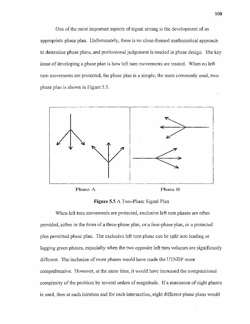
108
One of the most important aspects of signal setting is the development of an
appropriate phase plan. Unfortunately, there is no close-formed mathematical approach
to determine phase plans, and professional judgement is needed in phase design. The key
issue of developing a phase plan is how left turn movements are treated. When no left
turn movements are protected, the phase plan is a simple, the most commonly used, two-
phase plan is shown in Figure 5.5.
Phase A
Phase B
Figure 5.5 A Two-Phase Signal Plan
When left turn movements are protected, exclusive left turn phases are often
provided, either in the form of a three-phase plan, or a four-phase plan, or a protected
plus permitted phase plan. The exclusive left turn phase can be split into leading or
lagging green phases, especially when the two opposite left turn volumes are significantly
different. The inclusion of more phases would have made the UTNDP more
comprehensive. However, at the same time, it would have increased the computational
complexity of the problem by several orders of magnitude. If a maximum of eight phases
is used, then at each iteration and for each intersection, eight different phase plans would
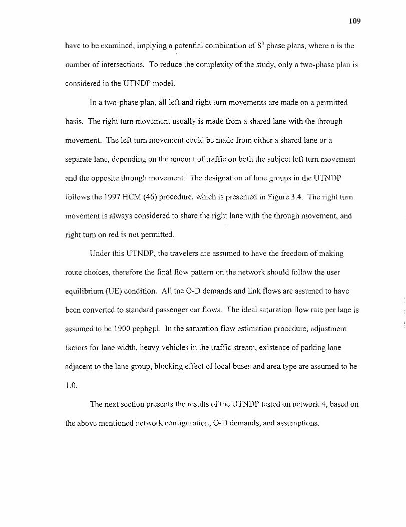
109
have to be examined, implying a potential combination of 8' phase plans, where n is the
number of intersections. To reduce the complexity of the study, only a two-phase plan is
considered in the UTNDP model.
In a two-phase plan, all left and right turn movements are made on a permitted
basis. The right turn movement usually is made from a shared lane with the through
movement. The left turn movement could be made from either a shared lane or a
separate lane, depending on the amount of traffic on both the subject left turn movement
and the opposite through movement. The designation of lane groups in the UTNDP
follows the 1997 HCM (46) procedure, which is presented in Figure 3.4. The right turn
movement is always considered to share the right lane with the through movement, and
right turn on red is not permitted.
Under this UTNDP, the travelers are assumed to have the freedom of making
route choices, therefore the final flow pattern on the network should follow the user
equilibrium (UE) condition. All the O-D demands and link flows are assumed to have
been converted to standard passenger car flows. The ideal saturation flow rate per lane is
assumed to be 1900 pcphgpl. In the saturation flow estimation procedure, adjustment
factors for lane width, heavy vehicles in the traffic stream, existence of parking lane
adjacent to the lane group, blocking effect of local buses and area type are assumed to be
1.0.
The next section presents the results of the UTNDP tested on network 4, based on
the above mentioned network configuration, O-D demands, and assumptions.

110
5.3 Traffic Assignment/Traffic Control Results
The first part of this section presents the impact of cycle length on traffic performance,
where the best cycle length is chosen and used in the subsequent tests conducted. The
second part studies the results in terms of traffic performance, including a summary of
the UTNDP results, network-wide performance analysis and intersection-based
performance analysis. The last part of this section presents the signal performance
analysis, including a summary of signal setting results and a bandwidth analysis for 3
major arterials of network 4. Network 4 is used in this section as the base for the traffic
engineering analysis due to its relatively larger size in comparison to the other three
networks.
5.3.1 Impact of Cycle Length on Network Total Travel Time
In most urban signalized networks, the same cycle length is usually assigned to all
intersections of the same network to achieve better synchronization of the traffic signals
and the traffic movements. The most commonly used cycle length in urban signalized
networks ranges from 60 to 120 seconds. In this study, network 4 is solved repeatedly
with cycle lengths from 60 to 120 seconds at 5-second increments to locate the best cycle
length. Figure 5.6 presents the user equilibrium (UE) network total travel time for a
fixed level of demand at different cycle lengths.
111
60 70 80 93 103
110
120
tilde Length (son.)
Figure 5.6 UE Network Total Travel Time VS. Cycle Length (Test Network 4)
As seen from the above figure, the UE network total travel time increases steadily
with increases in the cycle length. The network total travel time increases from 687 to
906 Veh.-hours when cycle length increases from 60 seconds to 120 seconds, a 32%
increase. For most of the links in this 3 by 5 grid network, the v/c ratios are less than 1.0,
and the whole network can be considered as under-congested. For under-congested
networks, the longer the cycle length is, the less portion of green is used by traffic flow,
and therefore the total network travel time increases. For network 4, the optimal cycle
length is 60 seconds, which is applicable to all intersections in the network. It is noted
that shorter cycle lengths could produce better results. However, since some of the lane
groups started producing v/c ratios greater than 1.2, then the total UE network total travel
time would have been incorrect, since the 1994 HCM delay formula was calibrated for
v/c ratios up to 1.2.
112
5.3.2 Traffic Performance
The study of traffic performance is divided into four major sections. The first section
summarizes the traffic assignment results arid the optimal traffic control strategies,
including optimal left turn controls and lane designation controls. The second section
presents the network-wide traffic performance measures that describe the average
performance of an O-D pair of the network. The third section studies the travel speed on
each link, which is the intuitive measurement of traffic performance of individual links.
The last section studies the performance of each intersection based on the LOS and v/c
ratio criteria. Intersection performance is important not only because a significant
portion of travel time in an urban network is spent on waiting for green signals, but also
because it reflects the efficiency of traffic control strategies, such as signal settings and
left turn controls, which are the major concerns of this study. To demonstrate the
effectiveness of traffic control strategy optimizations, the results under the original
traffic, signal and network configuration condition (the original condition) before
optimization are also presented parallel to the results under the optimized traffic, signal
and network configuration condition (the final condition) in Table A.
To study the effectiveness of the UTNDP model under different O-D demand
levels, the program was also run at 10% and 50% of the original O-D matrix. The 10%
original O-D demand condition represents a near free flow condition because the O-D
demands are very light, ranging from 3 to 9 vehs./hour. The 50% original O-D demand
condition represents a less congested condition compared with the original O-D demand
condition. The results under these three O-D plans are presented in Table B in Appendix
B.
113
5.3.2.1 Summary of Traffic Assignment Results and Optimal Traffic Control
Strategies: Based on the given O-D matrix and the network 4 configuration, the UTNDP
was solved using the SA-TABU search procedure. The results include the optimal
intersection turning movement control that governs where left turn movements should be
prohibited, the optimal lane designation scheme which dictates in which direction of a
link an additional lane is needed to accommodate peak traffic flows, and the optimal link
flows which are assigned to the network based on the optimal network configuration. The
results are summarized in in Table A Appendix A. Column two of Table A shows the
average link flows that represent the UE link flow pattern, and column three presents
corresponding average link delay for each link of the network. Left turns could either be
permitted or prohibited to eliminate conflicting flows, and potentially reduce the network
UE total travel time. The number of lanes in the original network is always 2, while in
the final network, the number of lanes on some links could increase from 2 to 3 or
decrease from 2 to 1. The link v/c ratios are also shown in Appendix A, as an index of
link congestion.
As seen in Table A in Appendix A, under the final condition, the average
movement based delays occurred at intersections range from 3.9 sec./veh. to 168.1
sec./veh. Most of the large delays are experienced by left turn movements, such as left
turn movement (133-130), (141-138), (53-50), (145-150) and (121-126), which are larger
than 60 seconds per vehicle. These large left turn delays 'force' the travelers to choose
another path to go to their destinations. For example, for a traveler who needs to make a
left turn via link (133-130), s/he would rather go through via (133-136) whose delay of
114
18.6 sec. /veh., is much less than the delay on left turn link (133-130), which is 168.1
sec./veh. The traveler will then make a left turn at the next intersection and then loop
around to his/her destination, if necessary. The large delays at the left turn links are
primarily due to the heavy conflicting traffic on opposite through links. Heavy
conflicting flows make it difficult for left turn vehicles to find acceptable gaps to
complete the turn, and therefore increases their delays. For example, links (133-130) and
(141-138), which have the highest average delays, conflict with heavy opposite through
flows, 1156 and 1214 vph on links (129-132) and (137-140), respectively.
Left turn movements from node 65 to 70, 97 to 102, 105 to 110 are prohibited.
The number of lanes of link (100-105) is reduced from 2 lanes to 1 lane, while the
opposite link (112-101) increases from 2 lanes to 3 lanes. Since link (100-105) only has 1
lane, left turn vehicles will block the through and right turn vehicles behind them if the
left turn movement is permitted on the link, and the delay of both the left turn vehicles
and the through and right turn vehicles Will increase significantly. In the UTNDP model,
the permission/prohibition of left turn movement at an intersection is based primarily on
the delay and v/c ratio of the subject link and its relevant links. If a left turn movement is
allowed on link (100-105), the delay and v/c ratio on link (100-105) increase
significantly, and thus link (100-105) becomes an appropriate candidate for left turn
prohibition. This observation reflects an important feature of the UTNDP that every
single link in a network is not an isolated individual link but a member of a number of
paths. The number of lanes on link (112-101) is increased from 2 lanes to 3 lane because
the HEF value of link (112-101) is large. The large HEF value of link (112-101) is
caused by the heavy traffic flow on the link (1401 vph), as opposed to the much lighter
115
traffic flow on the opposite link (100-105) (825 vph). Re-designation of the number of
lanes on this link can better accommodate traffic in the peak direction, and thus reduce
the network-wide travel time.
Volume to capacity ratio of a link is another important index of traffic. In the test
network, v/c ratios are calculated for all regular links, and the results are summarized in
Appendix A in Table A. Links (52-57), (100-105) and (132-137) exhibit v/c ratios
greater than 1.0. Consistently, large average travel times are found on links (52-57) and
(132-137). Among all the regular links, links (132-137) and (52-57) have the largest
average travel times, 64.3 and 63.1 sec./veh., respectively. Although link (100-105) has
high v/c ratio, the corresponding travel time on it is not as large, because the traffic flow
is only 825 vph. The higher v/c ratio is caused by the reduction of 1 lane from link (100-
105).
The total network travel time of network 4 has been reduced from 708.7 veh.-
hours under the original condition to 686.8 veh.-hours under the final condition, a 3.1%
decrease (see Table 5.6). The v/c ratios have been reduced on 23 of the regular links,
increased on 20 links, and unchanged on 1 link. The number of over congested regular
links with v/c ratios greater than 1.0 has been reduced from 4 under the original condition
to 3 under the final condition.
The traffic assignment and traffic control optimization results under the three O-D
plans are presented in Table B in Appendix B.
The v/c ratios have been reduced significantly with the decrease in the O-D
demand. The O-D ratios ranges from 0.01 to 0.18, and from 0.19 to 0.66 for the case of
10% and 50% of the original O-D demands, respectively, as opposed to from 0.38 to 1.13
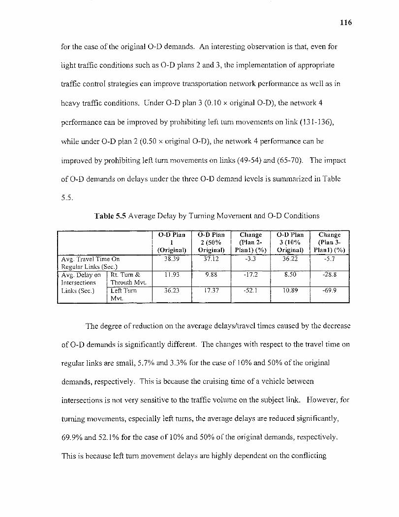
116
for the case of the original O-D demands. An interesting observation is that, even for
light traffic conditions such as O-D plans 2 and 3, the implementation of appropriate
traffic control strategies can improve transportation network performance as well as in
heavy traffic conditions. Under O-D plan 3 (0.10 x original O-D), the network 4
performance can be improved by prohibiting left turn movements on link (131-136),
while under O-D plan 2 (0.50 x original O-D), the network 4 performance can be
improved by prohibiting left turn movements on links (49-54) and (65-70). The impact
of O-D demands on delays under the three O-D demand levels is summarized in Table
5.5.
Table 5.5 Average Delay by Turning Movement and O-D Conditions
O-D Plan1
(Original)
O-D Plan2 (50%
Original)
Change(Plan 2-
Plan!) (%)
O-D Plan3 (10%
Original)
Change(Plan 3-
Plan!) (%)
Avg. Travel Time OnRegular Links (Sec.)
38.39 37.12 -3.3 36.97 -5.7
Avg. Delay onIntersectionsLinks (Sec.)
Rt. Turn &Throuth Mvt.
11.93 9.88 -17LT2 8.50 -28.8
Left TurnMvt.
36.23 17LT37 -52.1 10LT89 -69.9
The degree of reduction on the average delays/travel times caused by the decrease
of O-D demands is significantly different. The changes with respect to the travel time on
regular links are small, 5.7% and 3.3% for the case of 10% and 50% of the original
demands, respectively. This is because the cruising time of a vehicle between
intersections is not very sensitive to the traffic volume on the subject link. However, for
turning movements, especially left turns, the average delays are reduced significantly,
69.9% and 52.1% for the case of 10% and 50% of the original demands, respectively.
This is because left turn movement delays are highly dependent on the conflicting
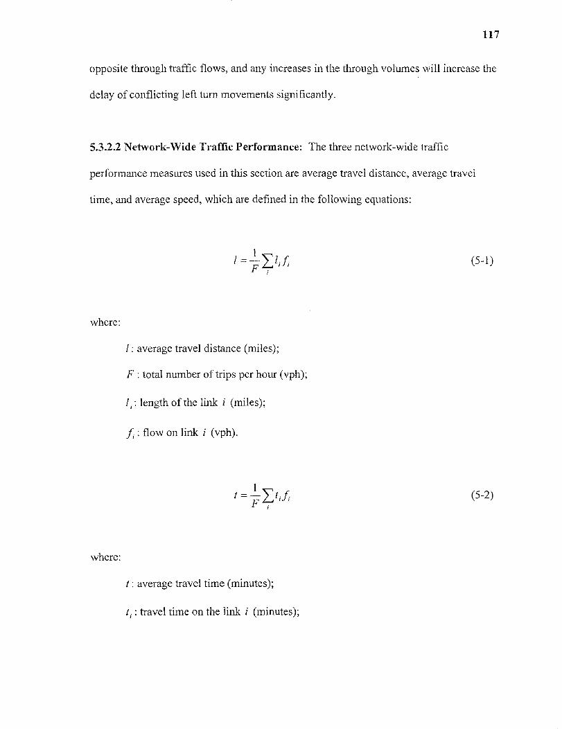
117
opposite through traffrc flows, and any increases in the through volumes will increase the
delay of conflicting left turn movements significantly.
5.3.2.2 Network-Wide Traffic Performance: The three network-wide traffic
performance measures used in this section are average travel distance, average travel
time, and average speed, which are defined in the following equations:
(5-1)
where:
1: average travel distance (miles);
F: total number of trips per hour (vph);
1.: length of the link i (miles);
f : flow on link i (vph).
1t = —
F(5-2)
where:
I : average travel time (minutes);
t, : travel time on the link i (minutes);
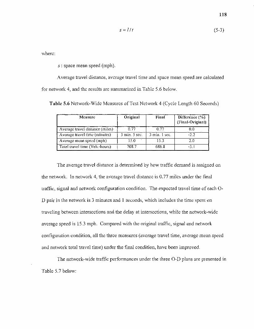
118
s = //t (5-3)
where:
s : space mean speed (mph).
Average travel distance, average travel time and space mean speed are calculated
for network 4, and the results are summarized in Table 5.6 below.
Table 5.6 Network-Wide Measures of Test Network 4 (Cycle Length 60 Seconds)
Measure Original Final Difference (%)(Final-Original)
Average travel distance (miles) 0.77 0.77 0.0Average travel time (minutes) 3 min. 5 sec. 3 min. 1 sec. -2.2
Average mean speed (mph) 15.0 15.3 2.0
Total travel time (VehLT-hours) 708.7 686.8 -3.I
The average travel distance is determined by how traffic demand is assigned on
the network. In network 4, the average travel distance is 0.77 miles under the final
traffic, signal and network configuration condition. The expected travel time of each O-
D pair in the network is 3 minutes and 1 seconds, which includes the time spent on
traveling between intersections and the delay at intersections, while the network-wide
average speed is 15.3 mph. Compared with the original traffic, signal and network
configuration condition, all the three measures (average travel time, average mean speed
and network total travel time) under the final condition, have been improved.
The network-wide traffic performances under the three O-D plans are presented in
Table 5.7 below:

119
Table 5.7 Network-Wide Measures of Test Network 4 (Cycle Length 60 Seconds)Under Three O-D plans
Measure 0-D Plan 1(Original)
0-D Plan 2 (50%) O-D Plan 3 (10%)
Average travel distance (miles) 0.77 0.77 0.77Average travel time (minutes) 3 min. 1 sec. 2 min. 37 sec. 2 min. 25 sec.
Average mean speed (mph) 15.3 17.6 19.I
Total travel time (Veh.-hours) 686.8 305.9 56.9
The average travel distance remains the same for all the three O-D plans, while
the other three measures vary signifrcantly. As the O-D demands decrease from the
original demand to 10% and then to 50% of the original demands, the average travel time
decreases as well, from 3 minutes 1 second to 2 minutes 37 seconds and then to 2 minutes
25 seconds. In the mean time, the average mean speed increases from 15.3 mph to 17.6
(0.5 x O-D) mph and then to 19.1 (0.1 x O-D) mph. The total network travel time has
been changed even more significantly, from 686.8 veh.-hours to 305.9 veh.-hours and
then to 56.9 veh.-hours. This is caused by the reduction in O-D demand, which
consequently reduces the average travel time of an individual vehicle.
5.3.2.3 Link Travel Speeds: As a major network-wide performance indicator, travel
speed can be studied in depth by investigating the spatial distributions of link travel
speeds. For regular links, travel time is computed as the cruise time plus the
corresponding through movement delay, and travel speed is then computed using the link
length and the calculated travel time. The results for the link travel speeds are
summarized in Table 5.8. The link space mean speeds under the three O-D plans are
presented in Table 5.9.

Table 5.8 Link Space Mean Speeds of Test Network 4 (Cycle Length 60 Seconds)
Node 1 Link Length Link Space Mean Speed (mph)Starting Ending (mi) Original Final
36 41 0.3 18.9 20.138 75 0.1 16.8 16.744 49 0.2 15.5 17.446 83 0.1 12.8 13.248 37 0.3 19.3 17.752 57 0.4 16.9 20.154 91 0.1 16.2 14.656 45 0.2 11.9 16.260 65 0.2 15.3 16.662 99 0LTI 13.3 13.264 53 0.4 18.1 20LT170 107 0.1 15.3 15.172 61 0.2 14.4 20.974 39 0.I 9.0 12.576 81 0.3 19.0 19.178 115 0.3 19.I 18.582 47 0.1 14.6 17.484 89 0.2 18LTI 18.386 123 0.3 19.I 18.788 77 0.3 18.9 20.290 55 0.1 13.3 13.892 97 0.4 18.3 18.894 131 0.3 20.6 20.396 85 0.2 17.5 17LT798 63 0.I 16.5 14.1100 105 0.2 18.0 14.I102 139 0.3 19.9 19.0104 93 0.4 17.2 19.7106 71 0.I 11.1 10.7110 147 0.3 18.2 19.2112 101 0.2 17.I 18.4114 79 0.3 17.5 17.8116 121 0LT3 18.5 18.3122 87 0LT3 20.2 20.2124 129 0.2 18.5 17.6128 117 0.3 19.7 19.7130 95 0LT3 19.6 18.4132 137 0.4 14.9 13.3136 125 0LT2 16.3 17.3138 103 0.3 20.5 20.9140 145 0LT7 16LT9 15.7144 133 0.4 17.9 18.2146 111 0.3 19.5 18.7
152 141 0.2 17.6 17.6
120
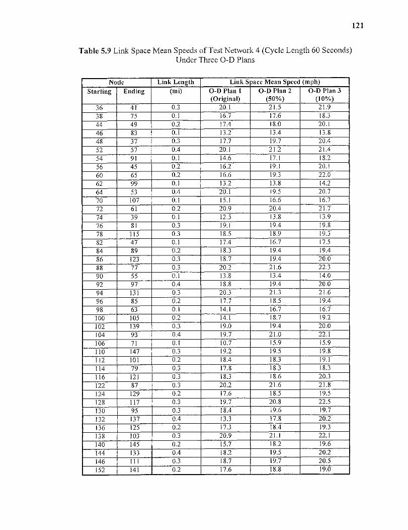
Table 5.9 Link Space Mean Speeds of Test Network 4 (Cycle Length 60 Seconds)Under Three O-D Plans
Node Link Length Link Space Mean Speed (mph)
Starting Ending (ml) O-D Plan 1(Original)
O-D Plan 2(50%)
0-D Plan 3(10%)
36 41 0.3 20.1 21.5 21.938 75 0.I 16.7 17.6 18.344 49 0.2 17.4 18.0 20.I46 83 0.1 13.9 13.4 13.848 37 0.3 17.7 19.7 20.452 57 0.4 20.1 21LT2 21.4
54 91 0.1 14.6 17.I 18.256 45 0.9 16.2 19.1 20.1
60 65 0.9 16.6 19LT3 22.062 99 0.I 13.2 13LT8 14.264 53 0.4 20.1 19.5 20.770 107 0.1 15.1 16.6 16.772 61 0.2 20.9 20.4 21.774 39 0.1 12.5 13.8 13.976 81 0.3 19.1 19.4 19.878 115 0.3 18.5 18.9 19.382 47 0.I 17.4 16LT7 17LT584 89 0.2 18.3 19.4 19LT486 123 0.3 18.7 19LT4 20LT0
88 77 0LT3 20.2 21LT6 22.390 55 0.1 13.8 13.4 14.092 97 0.4 18.8 19.4 20.094 131 0.3 20.3 21.3 21LT696 85 0.2 17.7 18.5 19.4
98 63 0.I 14.I 16.7 16.7100 105 0LT2 14.I 18.7 19.2102 139 0.3 19.0 19.4 20.0104 93 0.4 19.7 21LT0 22.I106 71 0.I 10.7 15.9 15.9110 147 0.3 19.2 19.5 19.8112 101 0.2 18.4 18.3 19.I114 79 0.3 17.8 18.3 18.3116 121 0.3 18.3 18LT6 20.3122 87. 0.3 20.2 21.6 21.8124 129 0LT2 17.6 18.5 19.5
128 117 0.3 19.7 20.8 22.5130 95 0.3 18.4 19.6 19.7132 137 0.4 13.3 17.8 20.2136 125 0.2 17.3 18.4 19.3138 103 0.3 20.9 21.I 22.1140 145 0.2 15.7 18.2 19.6144 133 0.4 18.2 19.5 20.2146 111 0.3 18.7 19.7 20.5152 141 0LT2 17.6 18.8 19.0
121

0-15 mph15--20 mph20--25 mph
0.1m 0.3m
122
Compared with the original O-D demand matrix, link space mean speeds
increased on 22 of the regular links, decreased on 19 links, and remained the same on 3
links, in the final condition. The network-wide space mean speed improved from 15.0
mph to 15.3 mph.
Link travel speeds are divided into 3 groups, below 15 mph, between 15 and 20
mph, and between 20 and 25 mph. Figures 5.7 and 5.8 depict the spatial distribution of
link travel speeds of network 4 for the final and original conditions, respectively.
Figure 5.7 Spatial Distribution of Link Space Mean Speeds for Network 4 (Cycle Length60 Seconds) Under the Final Condition

0.1m 0.3m
0-15 mph15--20 mph20--25 mph
0.4
Figure 5.8 Spatial Distribution of Link Space Mean Speeds for Network 4 (Cycle Length60 Seconds) Under the Original Condition
Under the final condition, out of the 44 regular links in the network, eight links
have space mean speeds less than 15 mph; eight links have speeds greater than 20 mph,
and the remaining 18 links have speeds ranging between 15 and 20 mph. Almost all of
the low speed links are located on the left side of the network. This is because these links
are relatively shorter and turning delays on these short links occupy a larger portion of
travel times on these links. One exception is the slow speed from intersection 13 to 14,
or on link (132-137) on the expanded network. The slow speed from intersection 13 to
14 is primarily due to the heavy traffic flow on it (1770vph).
123
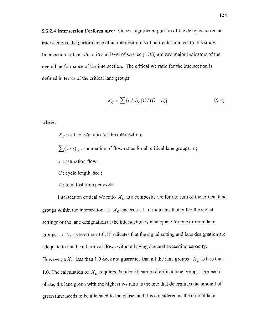
124
5.3.2.4 Intersection Performance: Since a significant portion of the delay occurred at
intersections, the performance of an intersection is of particular interest to this study.
Intersection critical v/c ratio and level of service (LOS) are two major indicators of the
overall performance of the intersection. The critical v/c ratio for the intersection is
defined in terms of the critical lane groups:
E(v/s),[C/ (c - (5-4)
where:
Cc : critical v/c ratio for the intersection;
E (,/ s) : summation of flow ratios for all critical lane groups, i ;
s : saturation flow;
C: cycle length, sec.;
L : total lost time per cycle.
Intersection critical vic ratio X (. is a composite v/c for the sum of the critical lane
groups within the intersection. If Xc exceeds 1.0, it indicates that either the signal
settings or the lane designation at the intersection is inadequate for one or more lane
groups. If Xc is less than 1.0, it indicates that the signal setting and lane designation are
adequate to handle all critical flows without having demand exceeding capacity.
However, a Cc less than 1.0 does not guarantee that all the lane groups' Cc is less than
1.0. The calculation of Xc requires the identification of critical lane groups. For each
phase, the lane group with the highest v/s ratio is the one that determines the amount of
green time needs to be allocated to the phase, and it is considered as the critical lane
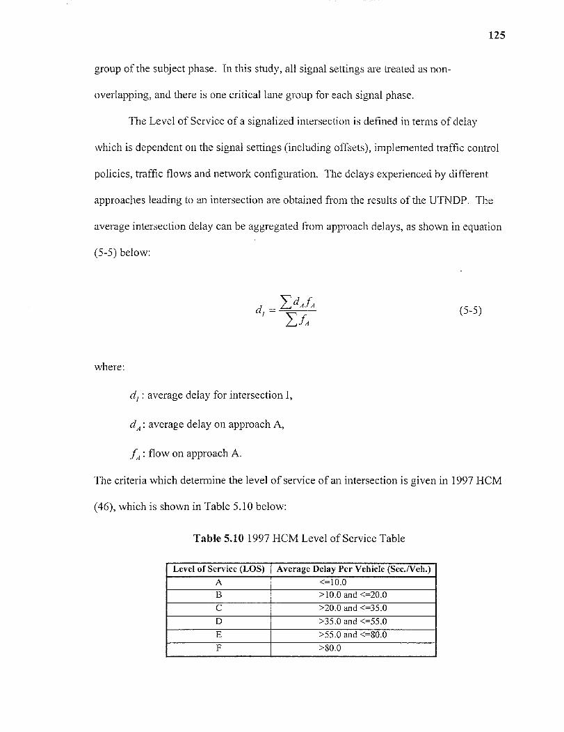
125
group of the subject phase. In this study, all signal settings are treated as non-
overlapping, and there is one critical lane group for each signal phase.
The Level of Service of a signalized intersection is defined in terms of delay
which is dependent on the signal settings (including offsets), implemented traffic control
policies, traffic flows and network configuration. The delays experienced by different
approaches leading to an intersection are obtained from the results of the UTNDP. The
average intersection delay can be aggregated from approach delays, as shown in equation
(5-5) below:
d fd = A A
Efa(5-5)
where:
average delay for intersection I,
dA : average delay on approach A,
fA flow on approach A.
The criteria which determine the level of service of an intersection is given in 1997 HCM
(46), which is shown in Table 5.10 below:
Table 5.10 1997 HCM Level of Service Table
Level of Service (LOS) Average Delay Per Vehicle (Sec./Veh.)
A <=10.0B >10.0 and <=20.0
C >20.0 and <=35.0
D >35.0 and <=55.0
E >55LT0 and <=80.0
F >80.0
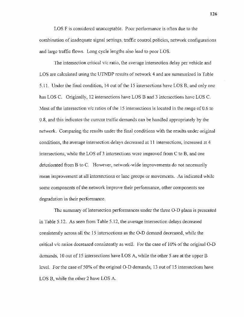
126
LOS F is considered unacceptable. Poor performance is often due to the
combination of inadequate signal settings, traffrc control policies, network configurations
and large traffic flows. Long cycle lengths also lead to poor LOS.
The intersection critical vie ratio, the average intersection delay per vehicle and
LOS are calculated using the UTNDP results of network 4 and are summarized in Table
5.11. Under the final condition, 14 out of the 15 intersections have LOS B, and only one
has LOS C. Originally, 12 intersections have LOS B and 3 intersections have LOS C.
Most of the intersection v/c ratios of the 15 intersections is located in the range of 0.6 to
0.8, and this indicates the current traffic demands can be handled appropriately by the
network. Comparing the results under the final conditions with the results under original
conditions, the average intersection delays decreased at 11 intersections, increased at 4
intersections, while the LOS of 3 intersections were improved from C to B, and one
deteriorated from B to C. However, network-wide improvements do not necessarily
mean improvement at all intersections or lane groups or movements. As indicated while
some components of the network improve their performance, other components see
degradation in their performance.
The summary of intersection performances under the three 0-D plans is presented
in Table 5.12. As seen from Table 5.12, the average intersection delays decreased
consistently across all the 15 intersections as the O-D demand decreased, while the
critical v/c ratios decreased consistently as well. For the case of 10% of the original 0-D
demands, 10 out of 15 intersections have LOS A, while the other 5 are at the upper B
level. For the case of 50% of the original O-D demands, 13 out of 15 intersections have
LOS B, while the other 2 have LOS A.
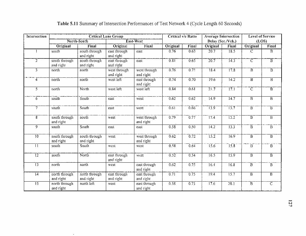
Table 5.11 Summary of Intersection Performances of. Test Network 4 (Cycle Length 60 Seconds)
Intersection Critical Lane Group Critical v/c Ratio Average IntersectionDelay (Sec./Veh.)
Level of Service(LOS)North-South East-West
Original Final Original Final Original Final Original Final Original Final1 south south through
and righteast throughand right
east 0.76 0.63 20.7 18.5
MIB
C BB
B
south throughand right
south throughand right
east throughand right
east 0.81 0.65 20.7 14.3
3 north north west throughand right
west throughand right
0.76 0LT71 18.4 17.8
4 north north west left east throughand right
0.74 0.70 19.6 14.2 B B
north North west left west left 0.84 0.61 21.7 17.1 C B
6 south South east west 0.62 0.62 14.9 14.7 B B
7 south South east west 0LT61 0.66 13LT9 13.7 B B
8 south throughand right
south west west throughand right
0.79 0.77 17.4 13.2 B B
9 south South east east 0.58 0.50 14.2 13.3 B B
10 south throughand right
south throughand right
west west throughand right
0.62 0.72 El= B B
south South west 0.58 0.64 15LT6 15.8 B111111
B12 south North east throughand right
west 0.52 0.54 16.5 15LT9 B
13 north north east throughand right
0.62 0.75 16.4 16.8 B B
14 north throughand right
north throughand right
east throughand right
east throughand right
0.71 0.75 19.4 B B
15 north throughand right
north left west east throughand right
0.58 0.73 17.6 28.1 B
Table 5.12 Summary of Intersection Performances of Test Network 4 (Cycle Length 60 Seconds) Under Three O-D Plans
IntersectIon 0-D Plan I (Original) O-D Plan 2 (50%) O-D Plan 3 (10%)
Crit. Ln. Grp. Crit. Avg, LOS Crit. Ln. Grp. Crit. Avg. LOS Crit. Ln. Grp. Crit. Avg. LOS
North-South
East-West
V/C Int.Del.
North-South
East-West
V/C Int.Del. '
North-South
East-West
V/C Int.Del.
s. thr.& rt.
east 0.63 18LT5 B south east 0.28 13.0 B south west 0.06 11.3 B
2 s. thr.& rt.
east 0.65 14.3 B south eLT thr.& rt.
0.62 10.0 B north eastleft
0.07 7.7
3 north w. thr.& rt.
0.71 17.8 B south w. thr.& rt.
0.46 13.3 B north w. thr.& rt.
0.10 10.3 B
4 north eLT thr.& rt.
0.70 14.2 B north e. thrLT& rt.
0.49 9LT9 A north eastleft
0.07 8.1 A
5 North westleft
0.61 17.1 B north w. thr.& rt.
0.31 10.I B north westleft
0.09 8.0 A
6 South west 0.62 14.7 B nLT thr.& rt.
west 0.41 10.4 B south west 0.06 8.5 A
7 South west 0.66 13.7 B south east 0.31 10.2 B south east 0LT07 8.7 A
8 south w. thr.& rt.
0.77 13.2 B south west 0.39 9.4 A south west 0.09 7.4 A
9 South east 0.50 13.3 B south east 0.30 10.5 B south east 0.07 7.0
10 s. thrLT& rt.
w. thr.& rtLT
0.72 16.9 B sLT thr.& rt.
east 0.37 11.7 B s. thr.& rtLT
west 0.05 9.7 A
11 South west 0.64 15LT8 B north e. thr.& rtLT
0.28 12.0 B north eastleft
0.06 10.9 B
12 North west 0.54 15.9 B north eLT thr.& rt.
0.43 12.7 B north eastleft
0.06 10LT4 B
13 north e. thr.& rt.
0.75 16.8 B north e. thr.& rt.
0.45 12.3 B south west 0.08 9.4 A
14 n. thr.& rtLT
e. thr.& rt.
0.75 15.7 B north e. thr.& rtLT
0LT46 11LT6 B north e. thr.& rt.
0.07 9.5 A
15 northleft
e. thr.& rt.
0.73 28.1 C northleft
west 0.40 13.1 B northleft
eLT thrLT& rt.
0.06 10.2 B
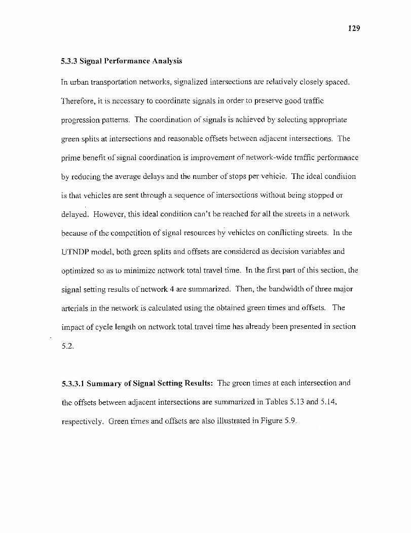
129
5.3.3 Signal Performance Analysis
In urban transportation networks, signalized intersections are relatively closely spaced.
Therefore, it is necessary to coordinate signals in order to preserve good traffic
progression patterns. The coordination of signals is achieved by selecting appropriate
green splits at intersections and reasonable offsets between adjacent intersections. The
prime benefit of signal coordination is improvement of network-wide traffic performance
by reducing the average delays and the number of stops per vehicle. The ideal condition
is that vehicles are sent through a sequence of intersections without being stopped or
delayed. However, this ideal condition can't be reached for all the streets in a network
because of the competition of signal resources by vehicles on conflicting streets. In the
UTNDP model, both green splits and offsets are considered as decision variables and
optimized so as to minimize network total travel time. In the first part of this section, the
signal setting results of network 4 are summarized. Then, the bandwidth of three major
arterials in the network is calculated using the obtained green times and offsets. The
impact of cycle length on network total travel time has already been presented in section
5.2.
5.3.3.1 Summary of Signal Setting Results: The green times at each intersection and
the offsets between adjacent intersections are summarized in Tables 5.13 and 5.14,
respectively. Green times and offsets are also illustrated in Figure 5.9.
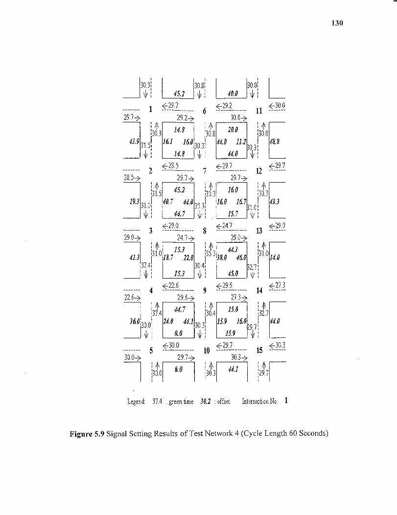
40.
-------
'30.0
30 3
12
;
7 29729LT7->
A ; t160130.3 :30.3160 167 I 43,3
310:15.7 v
30.8 20.0
44.0 11.2
44.0
-29.230.0->
14
HI'32.744.7
24.0 44.1
0.0
130.430LT31 4.0
130
30LT8
t'30LT3
45.2 V
29LT7->-29LT7
29LT2->14,8
43.9 31LT5 161 160 30.3V ; 14.8
28 52
28LT5-> 29.7->A
31LT5 45.219.3 31.01 40,7 44.0 35.3 V I 44,7
30 .3
29LT0->-29LT0 ÷24LT7 -29.0
324.7-> 29.0->
44.338.0 460
138
1 131.0
32 7;41.3
15.331.018.7 2Z0 135.3
37LT41 30LT4115.3 \b v45.0
4.0
<-22.622LT6-> 29.6->
A37LT4
360 300 1
30.0
30LT0-> 29.7->t 0 030LT0
15.0
15,9 160
15.9297v:
153() 3
27.39 -29LT6
27.3->
0 29LT7
30.3->
30.3 44.1
A
29LT7
Legend: 37LT4 : green time 30.2 : offset Intersection NoLT 1
Figure 5.9 Signal Setting Results of Test Network 4 (Cycle Length 60 Seconds)

131
There are two major constraints that dictate the green splits and offset setting.
First, green splits on each approach of an intersection should be long enough to
accommodate the traffic in that direction. In other words, the traffic demand on an
approach should not exceed the capacity allocated to the subject approach. The capacity
of the approach is determined by green splits, and geometric and traffic characteristics.
Second, the allocated green splits and offsets should satisfy the loop constraints. For
example, on loop 3-8-9-4-3, the summation of green splits and offsets should be equal to
the cycle length multiplied by an integer. In this case, the summation of green splits and
offsets of loop 3-8-9-4-3 is 180 seconds (15.3+24.7+22.0+30.4+15.3+22.6+18.7+31.0) or
3 cycle lengths.
Table 5.13 Green Splits at Intersections of Test Network 4 (Cycle Length 60 Seconds)
Intersection Effective Green (North-South)(Sec.)
Effective Green (East-West)(Sec.)
Original Final Original Final1 30.0 30.3 30.0 29.72 30LT0 31.5 30.0 28.53 30.0 31.0 30.0 29.04 30.0 37LT4 30LT0 22.65 30.0 30.0 30LT0 30.06 30.0 30.8 30LT0 29.27 30.0 29.7 30.0 30.38 30LT0 24LT7 30.0 35.39 30.0 30.4 30.0 29.610 30.0 30LT3 30.0 29.711 30.0 30LT0 30.0 30.012 30.0 30.3 30.0 29.713 30.0 29.0 30.0 31.014 30.0 32.7 30.0 27.315 30.0 29LT7 30.0 30.3
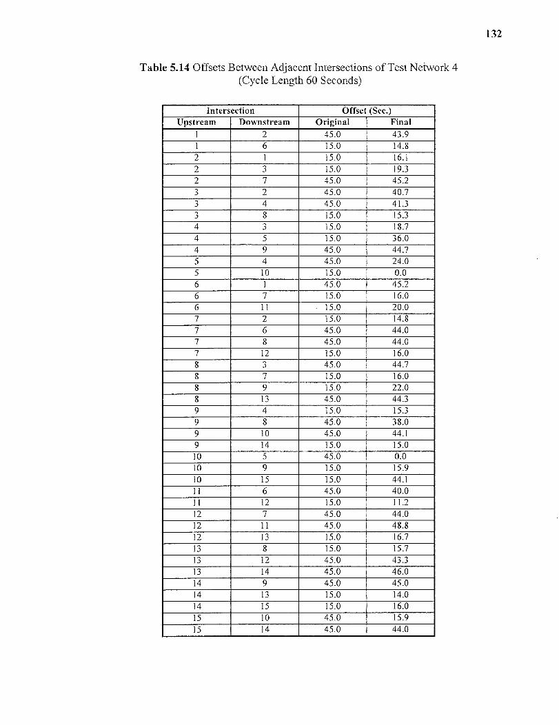
Table 5.14 Offsets Between Adjacent Intersections of Test Network 4(Cycle Length 60 Seconds)
Intersection Offset (Sec.)Upstream Downstream Original Final
1 2 45.0 43.91 6 15.0 14.82 1 15.0 16.12 3 15.0 19.32 7 45.0 45.23 2 45.0 40.73 4 45.0 41.33 8 15.0 15.34 3 15.0 18.74 5 15.0 36.04 9 45.0 44.75 4 45.0 24.05 10 15.0 0.06 1 45.0 45.26 7 15.0 16.06 11 15.0 20.07 2 15.0 14.87 6 45.0 44.07 8 45.0 44.07 12 15.0 16.08 3 45.0 44.78 7 15.0 16.08 9 15.0 22.08 13 45.0 44.39 4 15.0 15.39 8 45.0 38.09 10 45.0 44.I9 14 15.0 15.010 5 45.0 0.010 9 15.0 15.910 15 15.0 44.111 6 45.0 40.011 12 15.0 11.212 7 45.0 44.012 11 45.0 48.812 13 15.0 16.713 8 15.0 15.713 12 45.0 43.313 14 45.0 46.014 9 45.0 45.014 13 15.0 14.014 15 15.0 16.015 10 45.0 15.915 14 45.0 44.0
132

133
5.3.3.2 Bandwidths of Three Major Arterials: Bandwidth, which is often referred to as
the window of green through which platoons of vehicles can move, is an important
measure of signal efficiency of an arterial. Large bandwidth along an arterial reflects
good traffic progression. However, for a coordinated transportation network, a large
bandwidth in one direction of an arterial in the network is often selected by sacrificing
the signal efficiency in the opposite direction or on the adjacent arterials and streets. For
example, if the cross streets of the subject arterial have heavy traffic, the priority given to
the arterial through the signal settings may actually increase the network-wide total travel
time. Since the primary objective of this UTNDP model is the minimization of the
network-wide total travel time rather than the maximization of bandwidth on a particular
arterial, the bandwidth on some arterials in the network may not be optimal. The
bandwidths for the 3 vertical (north-south) arterials of network 4 under the final condition
are presented in Figures 5.10, 5.11, and 5.12, respectively. The bandwidth results under
both the original and the final conditions are summarized in Table 5.15.
Table 5.15 Bandwidth of 3 Major Arterials of Test Network 4
Arterial Direction Bandwidth(sec.)
Average Flow(veh./hour)
Original Final Original Final
1 I-2-3-4-5 (North-South) 0.0 11.6 1691 13315-4-3-2-1 (South-North) 0.0 I.8 1063 979
2 6-7-8-9-10 (North-South) 0.0 0.0 815 84310-9-8-7-6 (South-North) 3.6 6.7 1202 1338
3 11-12-13-14-15 (North-South) 0.0 0.0 1114 144315-14-13-12-11 (South-North) 0LT0 12.4 1016 964
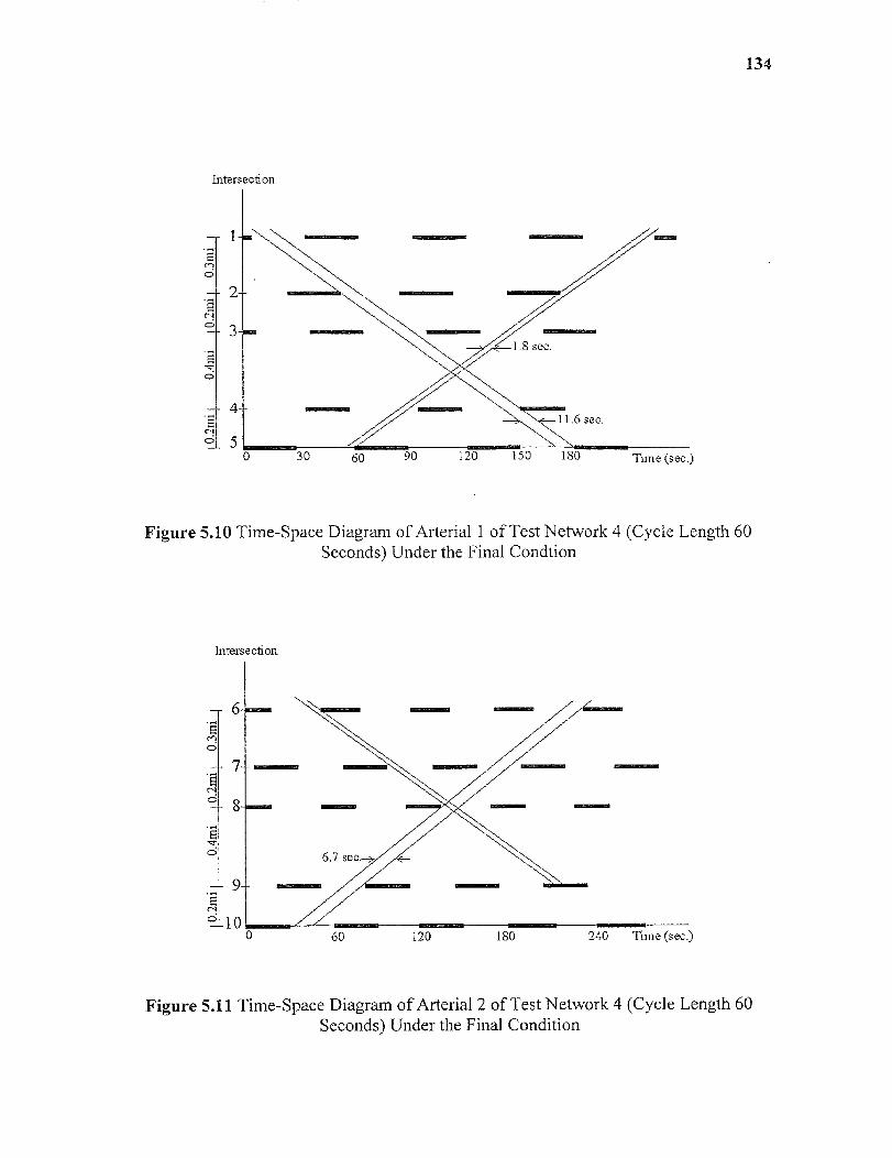
Intersection
Figure 5.10 Time-Space Diagram of Arterial 1 of Test Network 4 (Cycle Length 60Seconds) Under the Final Condtion
Intersection
134
.2
0 60
120
180
240
Time sec.)
Figure 5.11 Time-Space Diagram of Arterial 2 of Test Network 4 (Cycle Length 60Seconds) Under the Final Condition

0 60 120 180 240 Time (secLT)
Intersection
11
12
Figure 5.12 Time-Space Diagram of Arterial 3 of Test Network 4 (Cycle Length 60Seconds) Under the Final Condtion
Engineers usually wish to maximize bandwidth in the direction with heavy traffic,
while the other direction is largely ignored. More commonly, the bandwidths in the two
directions are designed to be in the same ratio as the flows in the two directions. Under
the final condition, the average flows in the north-south direction of arterial 1 and south-
north direction of arterial 2 are much heavier than the average flows in their opposite
directions, thus signal setting priorities should be given to these two heavy traffic
directions. Under the final condition, the bandwidths in the north-south direction of
arterial I and south-north direction of arterial 2 are 11.6 and 6.7 seconds, respectively, as
opposed to 1.8 and 0.0 seconds in the opposite directions. This is consistent with real
world engineering practices. However, this observation doesn't hold for arterial 3. This
might be due to the signal coordination constraints in a transportation network, such as
135
136
the loop constraints. The good signal progression on arterial 2 may lead to deteriorating
signal progression on an adjacent arterial such as arterial 3. Comparing the bandwidths
of the final and the original conditions, the bandwidths of the final condition are
consistently better than those of the original condition.

CHAPTER 6
PERFORMANCE OF THE SA-TABU HEURISTIC
The four test networks were subjected to the application of the heuristic search strategy in
solving the UTNDP. One of the most important elements of the SA-TABU search
procedure is the HEF (see equation 3.27), which is also presented below.
Heuristic Evaluation Function (HEF):
HEF, = ax(Vi / Ci)+bx HISCON, + c x RAND(0,1)
The HEF has three components, the link v/c ratio, the historical contribution
factor, and the random factor. The link v/c ratio reflects the performance of traffic on the
subject link under current solution set, the historical contribution factor reflects the
accumulated contribution of the current move since the start of the heuristic search
procedure, and the random factor is designed to enhance the stochastic nature of the
search procedure.
6.1 Summary of the Heuristic Search
Since the UTNDP solution procedure is a heuristic search procedure, the major
parameters of this procedure are discussed in this section, as they have significant impact
on the results. The three major types of parameters are: TABU list length, control
parameter (temperature) decreasing rate and Markov chain length, and the weight
coefficients of the three components of the HEF, namely the current link v/c ratio, the
historical contribution factor, and the random factor. A standard version of the heuristic
137
search strategy has been defined for comparison with other alternative versions. The
major parameters of the standard version include:
• TABU list length: 7,
• Markov Chain Length Increasing Rate: 20%,
• Initial Length of Markov Chain: 20,
• Control Parameter Decreasing Rate: 20%,
• Weight of Link V/C ratio: 1000.0
• Weight of Historical Contribution Factor: 1.0e-4,
Weight of Random Factor: 10.0
Other assumptions include:
• Maximum number of iterations of the SA-TABU search: 500,
• Maximum number of iterations of the Frank-Wolfe algorithm: 500,
• Maximum number of No-Change before program terminates: 50,
• Conversion criteria in the Frank-Wolfe algorithm: 0.0001,
• Number of major iterations in the non-linear programming procedure: 50,
• Number of minor iterations in the non-linear programming procedure: 2000,
• Accuracy of constraints in the signal setting procedure: 0.0001
A summary of the results subjected to the standard heuristic search for the four
test networks is presented in Table 6.1.
138
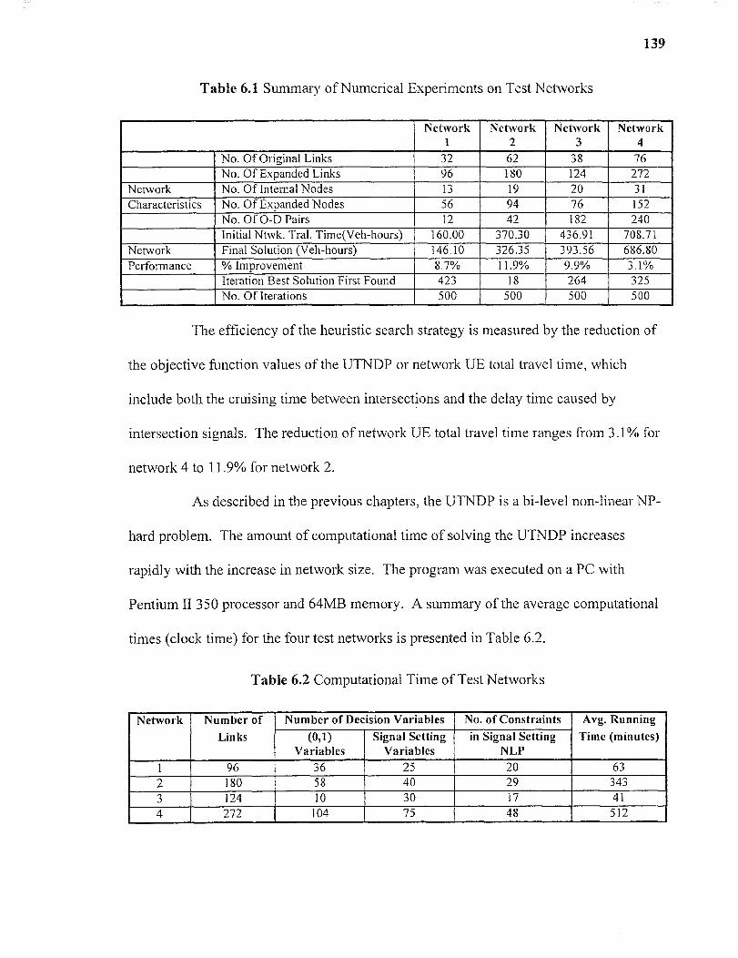
139
Table 6.1 Summary of Numerical Experiments on Test Networks
Network1
Network2
Network3
Network4
No. Of Original Links 32 62 38 76No. Of Expanded Links 96 180 124 272
Network No. Of Internal Nodes 13 19 20 31Characteristics No. Of Expanded Nodes 56 94 76 152
No. Of O-D Pairs 12 42 182 240Initial Ntwk. Tral. Time(Veh-hours) 160.00 370.30 436.91 708.71
Network Final Solution (Veh-hours) 146.10 326.35 393.56 686.80Performance % Improvement 8.7% 11.9% 9.9% 3.1%
Iteration Best Solution First Found 423 18 264 325NoLT Of Iterations 500 500 500 500
The efficiency of the heuristic search strategy is measured by the reduction of
the objective function values of the UTNDP or network UE total travel time, which
include both the cruising time between intersections and the delay time caused by
intersection signals. The reduction of network UE total travel time ranges from 3.1% for
network 4 to 11.9% for network 2.
As described in the previous chapters, the UTNDP is a bi-level non-linear NP-
hard problem. The amount of computational time of solving the UTNDP increases
rapidly with the increase in network size. The program was executed on a PC with
Pentium II 350 processor and 64MB memory. A summary of the average computational
times (clock time) for the four test networks is presented in Table 6.2.
Table 6.2 Computational Time of Test Networks
Network Number of
Links
Number of Decision Variables No. of Constraints Avg. RunningTime (minutes)(0,1)
VariablesSignal Setting
Variablesin Signal Setting
NLP
1 96 36 25 20 632 180 58 40 29 3433 124 10 30 17 414 272 104 75 48 512
140
The computational time increases 7.11 times from network 1 to network 4, while
the number of links of the networks only increases 1.83 times. The computational time
of these test networks is dictated by the number of decision variables in the
corresponding UTNDP, which include the (0,1) integer variables and continuous signal
setting variables. The (0,1) integer variables are the network configuration decision
variables, including the left turn control and land designation variables. The continuous
signal setting variables include green splits of the intersections in the network and the
offsets between each pair of adjacent intersections in the network. Although network 3
has more links than network 1, the computational time of network 3 is less than that of
network 1 because the number of (0,1) variables in network 3 is less than one third of
network 1.
6.2 Sensitivity Analysis on Major Algorithmic Parameters
The primary objective of sensitivity analysis is to investigate the impact of some key
parameters on the performance of the SA-TABU search procedure. For the simulated
annealing process, sensitivity is tested on the control parameter (temperature) decreasing
rate and the Markov chain length. A smaller control parameter decreasing rate and a
longer Markov chain length can lead to a more smoothing annealing process that yields a
good quality solution. However, it also requires a longer processing time. In order to
find a desirable solution within a reasonable amount of computational time, a
compromise needs to be made between the quality of the solution generated and the
processing time. The results of the sensitivity analysis on the control parameters, the
141
dropping rate and the Markov chain length can be used as guidance in making such a
compromise.
The TABU search procedure is used in the heuristic search to reduce the
occurrence of cycling and to avoid local optimal. The most recently made moves are
prevented from being updated again for certain number of iterations by placing them into
a TABU list. The length of the TABU list reflects the number of iterations a recently
updated variable needs to stay in the TABU list. The shorter the TABU list is, the larger
the possibility that the search will focus on a historically 'good' search region, with an
increased risk of the occurrence of cycles. The longer the TABU is, the larger the
possibility that the search is directed to a new search region, and therefore the less
opportunity the search is restrained to a local optimal, decreasing the risk of cycling.
The HEF places a value for each variable y, either abstract or real link of the
network, which identifies the move to be made at every iteration from one solution state
(network configuration) to the next. The HEF is composed of the current link v/c ratio,
historical link contribution factor, and a random factor generated by a random number
generator. The three elements are combined together linearly using weight coefficients
for each element. The current link v/c ratio reflects the current traffic performance on the
subject link, and the historical link contribution factor accumulates the impact of each
update of the subject lrnk on network-wide total travel time. The weight coefficients of
these three elements dictate which links are selected for updating at each iteration, and
thus have significant impact on the search procedure and the search results. The
sensitivity analysis on these weights provides a better understanding on how the three
HEF components affect the outcomes of the SA-TABU search procedure.
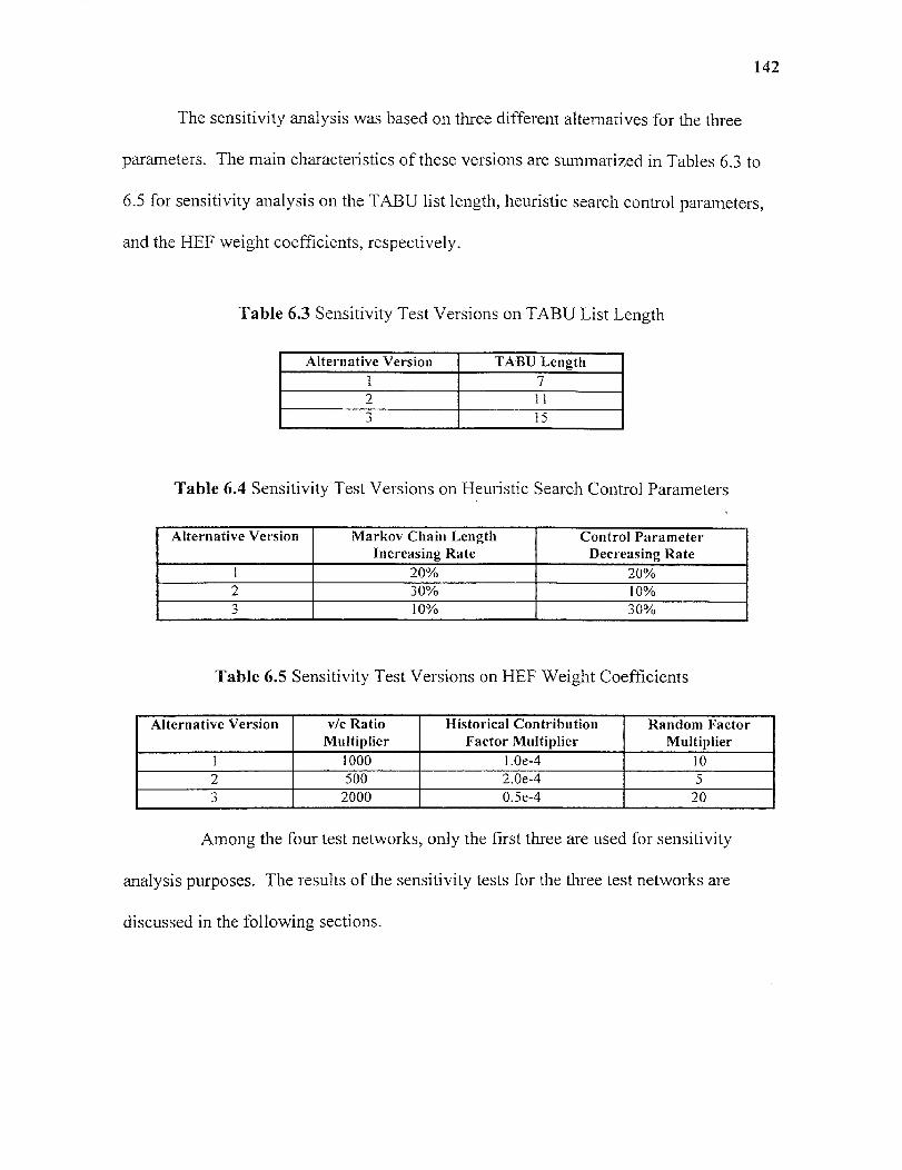
142
The sensitivity analysis was based on three different alternatives for the three
parameters. The main characteristics of these versions are summarized in Tables 6.3 to
6.5 for sensitivity analysis on the TABU list length, heuristic search control parameters,
and the HEF weight coefficients, respectively.
Table 6.3 Sensitivity Test Versions on TABU List Length
Alternative Version TABU Length1 72 H3 15
Table 6.4 Sensitivity Test Versions on Heuristic Search Control Parameters
Alternative Version Markov Chain LengthIncreasing Rate
Control ParameterDecreasing Rate
20% 20%2 30% 10%3 10% 30%
Table 6.5 Sensitivity Test Versions on HEF Weight Coefficients
Alternative Version v/c RatioMultiplier
Historical ContributionFactor Multiplier
Random FactorMultiplier
1 1000 I.0e-4 102 500 2.0e-4 53 2000 0.5e-4 20
Among the four test networks, only the first three are used for sensitivity
analysis purposes. The results of the sensitivity tests for the three test networks are
discussed in the following sections.
143
6.2.1 Sensitivity Tests on TABU List Length
The appropriate TABU list length depends primarily on the size and structure of the test
network. Glover (27) recommended using a length of 7, and this length is set as the
standard version in this study. Since the number of links in the three test networks are
fairly large after network expansion, the TABU list length needs to be set in a way that
most feasible solution regions are explored, while at the same time the search is detailed
enough in the local solution regions so that the search won't easily jump out of the local
region before a good local optimal is located, If the TABU list length is short, the 'good'
solution regions will appear repetitively during the search procedure, and other regions
are less likely to be explored. If the TABU list length is long, the explored trial region is
larger, however the 'good' solution regions are not as well explored as in the case of
short TABU list length. Because of the relatively large number of links on the expanded
networks, two alternative versions were explored with longer TABU list lengths, 11 and
15 respectively. The summaries of the sensitivity tests on the TABU list length are
presented in Table 6.6. The trial state and the current state performances of the TABU
list length of alternative version 1 of each test networks are presented in Figures 6.1 to
6.6. The following observations are made from Table 6.6.
• The mean of the trial solution states is always larger than that of the current solution
state, which reflects the selective nature of the SA-TABU search procedure. Only
trial solution states that meet the stochastic selection criteria in the simulated
annealing step in the SA-TABU procedure are accepted as current solution states.
144
• For all the three test networks, the means of total network travel time of both the
current solution state and the trial solution state decrease as the TABU list length
increases from 7 to 11, and then to 15. This may be because of the inappropriateness
of applying long TABU list length when the number of updateable variables is not
large enough, as it forces the search to a worse quality region when a significant
number of updateable links is put into the TABU list.
• Alternative version 1 produces the best results for all the three test networks. A
TABU list length of 7 is suggested for networks with limited updateable links, as
'good' solution regions need to be explored as much as possible before the search is
directed to another region. However, it is noted that more research should be
conducted on larger networks to find the most 'opt al' TABU list lengths.
6.2.2 Sensitivity Tests on Markov Chain Length and Control Parameter
The Markov chain length and the control parameter dictate the pattern of the simulated
annealing process. Besides the current solution state and the new solution state objective
functions, the temperature is the only factor in the acceptance criteria (see equation 3.29).
The temperature dictates the pace of the simulated annealing procedure. The larger the
temperature is, the easier the acceptance criteria are met. At the beginning of the search,
the temperature is usually set to a large value, and therefore most of the moves are
accepted. As the temperature is decreased at a fixed rate as the number of iterations
increases, only a few good solution states will be accepted. The larger the temperature
decreasing rate is, the more restrictive the SA-TABU search procedure is.

145
350 400 450 5000 50 100 150 200 250 300
Iteration
210.00
0 200.00
Z. 190.00
E180LT00
ra170.00
T1.1 j 160.00
150.00
140.00
Figure 6.1 Network UE Total Travel Time (Veh.-hours) VS. Iteration Number; (Network1, Alternative Version 1, Trial Solution State)
210
-0' 200
190
180
170
160
150
1400 50 100 150 200 250 300 350 400 450 500
Iteration
Figure 6.2 Network UE Total Travel Time (Veh.-hours) VS. Iteration Number; (Network1, Alternative Version 1, Current Solution State)
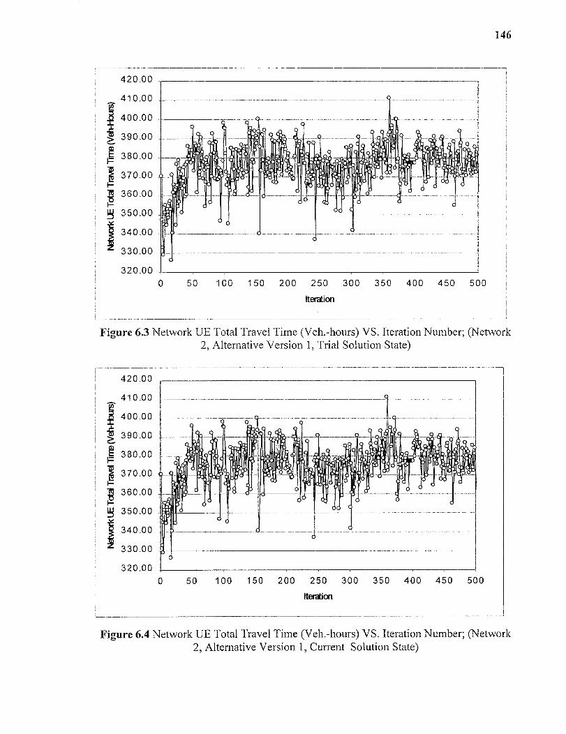
420.00
410LT00
400LT00
390LT00
380.00
370LT00
360.00
350.00
340.00
330.00
50 100 150 200 250 300 350 400 450 500 lteration
146
420.00
410LT00
400.00
390.00
380.00
370.00
360.00
350.00
340.00
330.00
320.00 0 50 100 150 200 250 300 350 400 450 500
Iteration
Figure 6.3 Network UE Total Travel Time (Veh.-hours) VS. Iteration Number; (Network2, Alternative Version 1, Trial Solution State)
Figure 6.4 Network UE Total Travel Time (Veh.-hours) VS. Iteration Number; (Network2, Alternative Version 1, Current Solution State)

480LT00E4.)
V. 7I— 15 440.00
E al °
50 100 150 200 250 300 350 400 450 500
Iteration
Figure 6.5 Network UE Total Travel Time (Veh.-hours) VS. Iteration Number; (Network3, Alternative Version 1, Trial Solution State)
147
500.00.L
480LT00
460.00a
E 440LT00°
48420.00E
400LT00
380.000 50 100 150 200 250 300 350 400 450 500
Iteration
Figure 6.6 Network UE Total Travel Time (Veh.-hours) VS. Iteration Number; (Network3, Alternative Version 1, Current Solution State)

148
The transformation from the current solution state to the subsequent solution state is
called a transition in the simulated annealing procedure. A transition consists of both the
application of acceptance criteria and the application of the generation mechanism, which
is used to generate a new solution state. Usually a number of transitions is generated
under a fixed temperature, and the number of transitions is determined by Markov chain
length. A large Markov chain length increasing rate and/or small temperature dropping
rate lead to a less restrictive search procedure that trial states are more easily to be
accepted. Consequently, the search region is widened and the search quality is improved.
However, this also leads to a slower progressing speed, and it creates a significant
disadvantage on the efficiency of the algorithm. On the other hand, a small Markov
chain length increasing rate and/or large temperature dropping rate lead to a faster search
procedure, but it also narrows down the search region and increases the risk of ending the
search procedure at an undesirable local optimal. Compared with the alternative version
1, alternative version 2 represents a less restrictive and slower search procedure, while
alternative version 3 represents a more restrictive and faster search procedure. The results
of the sensitivity tests on Markov chain length and temperature are summarized in Table
6.7. The following observations are noted from Table 6.7.
• The mean of the network total travel time of the trial solution states is always larger
than that of the current solution state, which reflects the selective nature of the SA-
TABU search procedure.
• For all the three test networks, the mean of both the current state and the trial state
decreases from alternative version 2 to alternative version 1 and to alternative version

149
3, which reflects the fact that a large Markov increasing rate and for small
temperature dropping rate are less restrictive in moving from one iteration to the next.
• Alternative version 3 produces the best results of all the three test networks. For all
the three networks, the feasible solution spaces are relatively large after network
expansion, and a faster and less restrictive global search such as alternative version 3
help to locate a better solution state rather than a slower narrow local search such as
alternative version 2.
6.2.3 Sensitivity Tests on the Heuristic Evaluation Function (HEF) Coefficients
The HEF has three components, the current v/c ratio, the historical contribution factor,
and the random factor. The selection of move to be made and link(s) to enter/exit the
current solution state, is significantly dependent on the weight of these three components.
If a larger weight is given to current link v/c ratios, the links with large v/c ratios are
more likely to be selected for updating so that the traffic performance can be improved.
If a larger weight is given to the historical contribution factor, then more emphasis is
given to the historical factor, and links that historically performed well are more likely to
be included in the final solutions. The random factor is included in the HEF so that the
search process is more stochastic, and the search explores a wider region, aiding to the
diversification of the search and jumping out of local optima. Compared with the
alternative version 1, alternative version 2 put more emphasis on the historical factor,
increasing the risk that some 'good' regions are expected to appear repetitively in the
search procedure. Alternative version 3 put more emphasis on the current link v/c ratio,
and the exploration of the solution regions is less restrictive. The results of sensitivity
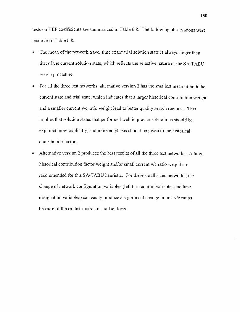
150
tests on HEF coefficients are summarized in Table 6.8. The following observations were
made from Table 6.8.
• The mean of the network travel time of the trial solution state is always larger than
that of the current solution state, which reflects the selective nature of the SA-TABU
search procedure.
• For all the three test networks, alternative version 2 has the smallest mean of both the
current state and trial state, which indicates that a larger historical contribution weight
and a smaller current v/c ratio weight lead to better quality search regions. This
implies that solution states that performed well in previous iterations should be
explored more explicitly, and more emphasis should be given to the historical
contribution factor.
• Alternative version 2 produces the best results of all the three test networks. A large
historical contribution factor weight and/or small current v/c ratio weight are
recommended for this SA-TABU heuristic. For these small sized networks, the
change of network configuration variables (left turn control variables and lane
designation variables) can easily produce a significant change in link v/c ratios
because of the re-distribution of traffic flows.

Table 6.6 Summary of Sensitivity Analysis on TABU List Length
Network AlternativeVersion
TABU ListLength
Best Solution Iterations Mean of Curt .Sol. State
Std. Dev. ofCurt. Sol. State
Mean of Tril.Sol. State
Std. Dev. ofTril. Sol. State
1
1 7 525965.1 423 645442 42533.95 657211.6 41997.99
2 11 542595.6 321 644451.6 40432.6 648595.3 39056.95
3 15 551552LT5 32 628411LT2 35019LT48 642426.6 38611.45
2
1 7 1174892 18 1351610 42323.42 1352800 42134.04
2 11 1184891 5 1381236 61496 1384620 61363.12
3 15 1184891 5 1362571 50893.86 1366642 5096 .63
3
1 5 1416825 264 1569203 56541.28 1579979 59609.26
2 7 1432352 393 1570481 63772.4 1576196 62552.47
3 9 1422733 432 1561972 57868.85 1570067 60186.52

Table 6.7 Summary of Sensitivity Analysis on Markov Chain Length and Control Parameter (Temperature)
Network AlternativeVersion
MarkovChain Incr.
Rate
Ctrl. Parm.Deer. Rate
Best Solution Iterations Mean of Curt. Sol. State
Std. Dev. ofCurt. Sol.
State
Mean of Tril.Sol. State
Std. Dev, ofTril. Sol.
State
1
1 20% 20% 525965.1 423 645442 42533.95 657211.6 41997.99
2 30% 10% 552796 4 664088.1 34174.47 668825.6 32637.84
3 10% 30% 505253.1 273 598240.1 42868.58 621770.4 41214.16
2
1 20% 20% 1174892 18 1351610 42323.42 1352800 42134.04
2 30% 10% 1174892 18 1355377 43165.33 1357732 43463.6
3 10% 30% 1145235 443 1340444 50563.87 1347850 49121.65
3
1 20% 20% 1416825 264 1569203 56541.28 1579979 59609.26
2 30% 10% 1416825 398 1583844 58838.67 1588553 59958.21
3 10% 30% 1405365 325 1555450 58930.76 1567207 55757.38
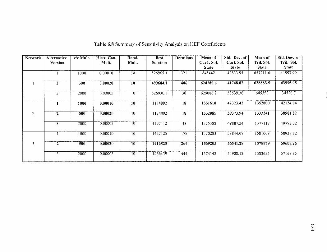
Table 6.8 Summary of Sensitivity Analysis on HEF Coeffrcients
Network AlternativeVersion
v/c Mult. Histr. Con.MuIt.
Rand.Mult.
BestSolution
Iterations Mean ofCurt . Sol.
State
Std. Dev. ofCurt. Sol.
State
Mean ofTril. Sol.
State
Std. Dev. ofTril. Sol.
State
1
1 1000 0.00010 10 525965.I 321 645442 42533.95 657211.6 41997.99
2 500 0.00020 10 499684.1 406 624180.6 41748.82 638883.5 43995.95
3 2000 0.00005 10 526930.8 30 629086.2 33539.36 645350 34520.7
2
1000 0.00010 10 1174892 18 1351610 42323.42 1352800 42134.04
2 500 0.00020 10 1174892 18 1332085 39373.94 1333341 38981.82
3 2000 0.00005 10 1197412 48 1375388 49887.34 1377 17 49798.02
3
1000 0.00010 10 1427125 178 1570283 58844.07 1581008 58937.82
2 500 0.00020 10 1416825 264 1569203 56541.28 1579979 59609.26
3 2000 0.00005 10 1466439 444 1574142 54908.13 1583655 57 68.85
CHAPTER 7
CONCLUSIONS AND FUTURE RESEARCH
7.1 Summary of the UTNDP
The motivation for this study stems from the need of alleviating traffic congestion in
urban transportation networks by implementing appropriate traffic control strategies.
These control strategies addressed in this UTNDP include signal setting control,
intersection left turn movement control and lane designation control. Appropriate
intersection left turn movement control can reduce conflicts caused by turning vehicles.
Re-designation of lanes can better accommodate peak direction traffic. An integrated
signal setting subroutine in the UTNDP can allocate signal resources more reasonably in
response to link flows and network configurations. The analogy between the network
design problem and the optimization of traffic control strategies motivates the
formulation of the UTNDP model to optimize traffic control strategies. The UTNDP
model is a bi-level nonlinear mixed integer programming model with the minimization of
network wide total travel time as its objective. On the upper level, the traffic control
strategies, intersection left turn control, lane designation and signal setting control are
optimized with fixed flows, while on the lower level, an asymmetric assignment is
conducted based on the current network configurations. Intersection left turn control and
lane designatron variables are discrete variables, while signal setting and link flows are
continuous variables. A realistic link delay estimation procedure, which follows the 1997
HCM (46) procedure, is used in the UTNDP model. Link delays not only depend on link
flows, but also depend on signal settings, network configurations, and traffic control
154
155
policies. The presence of link interactions leads to the asymmetric nature of the traffic
assignment step in the lower level of the UTNDP model, and it requires a diagonalization
procedure that takes into account the rmpact of conflicting link flows on the delay on the
subject link. A streamlined diagonalization procedure is used in solving the asymmetric
traffic assignment. The UTNDP is a NP-Hard problem, and the complexity of the
UTNDP makes it impossible to find the optimal solution. An iterative heuristic search
procedure is developed to solve the UTNDP model. The heuristic search procedure
developed in this study is SA-TABU procedure that combines the main characteristics of
the simulated annealing and TABU search procedures. The heuristic search is guided by
a heuristic evaluation function (HEF), which has three components, the current link v/c
ratio, the historical contribution factor and the random factor. To test the efficiency of
the solution procedure, four test networks are designed and used as the basis for the
numerical tests.
The major contributions of this dissertation includes:
• The formulation of a comprehensive Urban Transportation Network Design Problem
(UTNDP), which requires optimizations at the network structural level, signal setting
level and the traffic assignment level, is first of its kind. The UTNDP is formulated as
a bi-level nonlinear mixed integer programming problem, which can be used to select
the appropriate signal and traffic control strategies systematically. The interactive
nature between the signal and network configuration optimization and the traffic
assignment requires a model to integrate these two aspects together rather than solve
them separately. The design of the UTNDP model reflects the integration of these
two aspects.
156
• Development of an asymmetric traffrc assignment procedure to find link flows. The
existence of large amounts of intersection turnings in a urban transportation network
requires an asymmetrrc traffic assignment procedure to reflect the interaction of the
conflicting link flows. The diagonalization used in the traffic assignment procedure
is designed to account for the impact of conflicting opposite through traffic flows on
the delay of the subject left turn movement. This contribution is an extension of
Berka et al.'s (13) work, which first addressed this problem.
• Development of a realistic link delay estimation procedure which takes into account
link flows, signal settings, and network configurations. The complex nature of the
factors affecting link delays in an urban transportation network makes it inappropriate
to use BPR type curves as the link performance functions. A realistic link
performance function is designed to include signal settings and link flows as
dependant variables.
• Development of a heuristic search strategy to solve the UTNDP. The SA-TABU
search procedure is used to solve the UTNDP, which combines the major
characteristics of theTABU search and the Simulated Annealing search procedures.
The UTNDP results were obtained in reasonable amounts of time for all the 4 test
networks. To test the efficiency of the model and the solution procedure, numerical
tests need to be conducted on various sizes of test networks.
• Development of a signal setting optimization procedure that is integrated as part of
the UTNDP. As an essential part of the UTNDP, signal setting is critical to both the
optimizations of other traffic control strategies and the traffic assignments in the
157
network. Signal setting not only included green splits and cycle length as its decision
variables, but also included offsets as decision variables as well.
7.2 Conclusions
The following conclusions are made from this research:
The efficiency of urban transportation networks can be improved by implementing
appropriate traffic control strategies, such as intersection left turn control, lane
designation control, and signal timing control, without physical expansion of urban
streets. The network UE total travel time of the four test networks in this study were
reduced by 8.7%, 11.9%, 9.9% and 3.1% for networks 1, 2, 3 and 4, respectively. By
implementing intersection left turn control, conflicting flows are eliminated and thus
reduce network-wide total travel time. Redesignation of number of lanes can better
accommodate traffic in peak directions and thus alleviate peak direction congestion.
The introduction of a signal setting step in the UTNDP makes the model more
realistic, because the link flow and control strategy dependent signal setting scheme
can better reflect the signal requirement of traffic flows. The inclusion of offsets as
the signal setting variables can better reflect the coordinated nature of the signalized
urban transportation networks, although it also increases the complexity of the model
and the solution search procedure. On three major arterials in network 4, the
bandwidths, which are widely used by engineers as indices of signal coordination,
were improved after the signal and traffic control strategies were optimized.
• The realistic link delay functions used in this study, rather than the BPR type curves,
take into account the impact of signal setting and traffic control strategies on link
158
delays. This is consistent with the fact that large portion of delays occurred at
intersections rather than on traveling between intersections on urban networks.
Numerical test results have shown that, as the 0-D demand increases, the turning
movement delays, especially the left turn movement delays, increase significantly.
This demonstrated that the use of realistic delay functions in transportation modeling
is extremely important when the traffic flow is heavy in the subject transportation
network, such as an urban transportation network.
The asymmetric traffic assignment, which is solved by using the streamlined
diagonalization algorithm, can better represent the impact of conflicting flows on the
delay of the subject link. The conflicting pair of links on an urban network includes
the through movement and the left movement on the opposite direction, or vrce versa.
Because of the unprotected left turn phases at most intersections in an urban network,
the impact of conflicting flow on delay of the subject link can not be omitted.
Numerical tests have shown that delays occurring on intersection left turn links
occupy a large portion of the total delays on the network, which is especially true
when the traffic flow on the subject network is heavy.
• The cruise times between two adjacent intersections are not as sensitive to link
volumes as intersection turning movement delays to link volumes. The numerical test
on network 4 has shown that with a 50% decrease in 0-D demands, the average link
cruise time decreased only 3.3%, while the average left turn movement delays
decreased 52.1%.
• The implementation of appropriate signal, intersection turning, and lane designation
controls can improve traffic performances. For test network 4, the network-wide

159
average speed was improved from 15.0 mph to 15.3 mph, while the average travel
time of an O-D pair was reduced from 3 minutes 5 seconds to 3 minutes 1 seconds.
The number of over congested links with v/c ratios greater than 1.0 was reduced from
4 to 3.
The SA-TABU heuristic search procedure is an efficient search procedure in finding
near optimal solutions for the UTNDP. It combines the aggressive TABU search
characteristic with the conservative simulated annealing characteristic so that a
reasonable compromise is made between directing the search to a new solution region
and concentrating on the current search region. For the four test networks, acceptable
results were obtained in a reasonable period of time.
0 The three major components of the SA-TABU strategy are simulated annealing,
TABU search and the heuristic evaluation function (HEF). For the simulated
annealing process, a smaller control parameter decreasing rate and a longer Markov
chain length can lead to a more smoothing annealing process that yields a good
quality solution. However, it also requires a longer processing time. For the TABU
search procedure, the shorter the TABU list is, the larger the possibility that the
search will focus on a historically 'good' search region, with an increased risk of
cycling. The longer the TABU is, the larger the possibility that the search is directed
to a new search region, and therefore the less opportunity the search is restrained to a
local optimal, decreasing the risk of cycling. The weight coefficients of these three
elements dictate which links are selected for updating at each iteration, and thus have
significant impact on the search procedure and the search results.
160
e The amount of computational time of solving the UTNDP increases rapidly with the
increase in network size. The computational time increases 7.11 times from network
1 to network 4, while the number of links of the networks only increases 1.83 times.
7.3 Future Research
The two major traffic control strategies studied in this research are the intersection
left turn movement control and the lane designation. However, another important
control strategy needs to be addressed in future research is the selection of roads
which should implement one-way traffic control policies as opposed to two-way
traffic policies. The availability of paths between any 0-D pairs needs to be
carefully addressed if a one-way traffic policy is also considered.
• At the traffic assignment level, the 1994 HCM delay estimation model is used as the
link performance function, which include link flows and green splits, and cycle length
as its independent variables. The HCM model can not replace Gartner's model in the
signal setting level because offsets are not considered as independent variable in the
HCM formulation. On the other hand, Gartner's model can not replace the HCM
formulation because it can not be converted to movement based delay estimations,
which is essential in our application. This discrepancy needs to be resolved in the
future, and a consistent movement based delay estimation model needs to be
developed to include link flows, green splits, cycle length and offsets as the
independent variables.
• Because of the link capacity constraints in the signal setting step, only under-
congested conditions are addressed in this study. The formulation of the UTNDP

161
model under congested conditions needs to be studied in the future which requires a
modified signal setting model that can take into account congested traffic conditions.
• Eventually, the static UE traffic assignment used in this study should be replaced by a
more accurate dynamic traffic assignment that would better capture the user travel
behavior under dynamic changing conditions.
• The inclusion of offsets in the signal setting model introduces integer variables in the
loop constraints of a nonlinear programming model, and it increases the complexity
of the model significantly. In this study, only a limited number of major loop
constraints is included in the signal setting step for each test network. A more
accurate procedure needs to be developed to address the loop constraint issue.
• Other heuristic search procedures are recommended to explore the performance of the
search procedure, in particular, the techniques of neural network and genetic
algorithms. Extensive tests need to be conducted on larger networks to test the
efficiency of the search procedure.
• In future research, objectives other than network-wide total travel time could be
included in the objective function, such as fuel consumption, environmental impacts,
and multiple classes of users such as autos, trucks, buses etc.
• Since the computational demand of the UTNDP model is extensive, parallel-
computing techniques may need to be explored to increase the computatronal speed
APPENDIX A
SUMMARY OF UTNDP RESULTS OF TEST NETWORK 4
162

Table A Summary of UTNDP ResultsNode Average Flow
(veh./hour)Average Delay
(sec./veh.)No. of Lanes V/C ratio
Starting Ending Original Final Original Final Original Original Final Original33 38 148 287 26.6 33.6 Permitted Permitted 1 i n/a n/a33 36 572 433 14.3 n/a n/a n/a n/a n/a n/a33 34 60 60 15 14.3 n/a n/a n/a n/a n/a n/a35 40 45 45 15.4 26,5 Permitted Permitted n/a 1.111= n/a n/a
1111E1.1135 3836
354 315 15.9 11.5 n/a n/a n/a n/a n/a381 420 15.9 11.5 n/a n/a MEM n/a n/a n/a
36 41 1419 1154 47.I 46.2 n/a UM= 2 2 1LT09 0.8537 34 315 38 28LT5 Permitted Permitted ME= n/a n/a n/a
37 40 510 510 10.4 15.6 n/a n/a n/a n/aMal n/a
n/an/a
n/an/a111111111 38 198 45 10.4 15.6 n/a n/a
38 111111111111 701 647 15 14.9 n/a 2 2 0LT72 0.5139 36 466 301 33.6 33.9 Permitted Permitted n/a
EMIn/a n/a
n/an/an/a39 34 488 450 24.7 13.4 n/a n/a n/a
39 40 270 270 24.7 13LT4 n/a n/a n/a n/a n/a 1111=n/a41 46 105 40.I 27 Permitted Permitted n/a n/a n/a
41 44 1209 916 10 7LT4 n/a n/a n/a 11111121111=111111 n/a41 42 105 105 10 7.4 n/a n/a n/a n/a n/a n/a43 48 133 90 28.4 Permitted Permitted n/a n/a n/a n/a43 46 308 360 15.3 16.6 n/a n/a NEM n/a n/a n/a43 44 309 300 15.3 16LT6 n/a n/a n/a Ilia REM
n/a
n/a0-84n/a
44 49 1630 1335 31LT8 31.2 n/a n/aMEN111111111.1111.1111111111110111
n/a45 42 224 225 72.4 38LT4 Permitted Permitted45 48 807 690 29.6 14.1 n/a n/a n/a n/a n/a M12.
n/a45 46 99 45 29.6 14,1 n/a n/a n/a n/a Mal46 83 513 538 14LT8 14.8 n/a 2 2 0.38 0LT3847 44 111 120 23.9 Permitted Permitted n/a
n/an/a n/an/a
n/an/a47 42 510 9.7 n/a n/a
Table A (Continued)
47 48 46 90 9.7 5.7 n/a n/a n/a n/a n/a n/a48 37 985 870 45.7 45.4 n/a n/a 2 2 0.57 0.5549 54 59 150 61.9 37.5 Permitted Permitted n/a n/a n/a n/a49 52 1380 1035 14.8 10.I n/a n/a n/a n/a n/a n/a49 50 190 150 14.8 10.1 n/a n/a n/a n/a n/a n/a51 56 195 195 31.9 30.3 Permitted Permitted n/a n/a n/a n/a51 54 650 688 17.3 17.4 n/a n/a n/a n/a n/a n/a51 52 325 287 17LT3 17.4 n/a n/a n/a n/a n/a n/a52 57 1857 1502 64.8 63.I n/a n/a 2 2 I.15 1.1053 50 11 150 195 92.1 Permitted Permitted n/a n/a n/a n/a53 56 876 705 18 10 n/a nla n/a n/a n/a n/a53 54 270 263 18 10 n/a n/a n/a n/a n/a n/a54 91 978 1101 15.2 15.4 n/a n/a 2 2 0.74 0.7355 52 151 180 45.5 44.3 Permitted Permitted n/a n/a n/a n/a55 50 609 510 12 10.2 n/a n/a n/a n/a n/a nla55 56 59 60 12 10.2 n/a n/a n/a n/a n/a n/a56 45 1130 960 30.8 30.4 n/a n/a 2 2 0.66 0.6557 62 59 212 76.9 38LT6 Permitted Permitted n/a n/a n/a n/a57 60 1544 1095 20LT6 8LT4 n/a n/a n/a n/a n/a n/a57 58 254 196 20.6 8.4 n/a n/a n/a n/a n/a n/a59 64 280 254 34.1 40.9 Permitted Permitted n/a n/a n/a nla59 62 424 451 14.6 18LT8 n/a n/a n/a n/a n/a n/a59 60 121 120 14LT6 18.8 n/a n/a n/a n/a n/a n/a60 65 1859 1336 32.4 31.2 n/a n/a 2 2 1.10 0.6461 58 112 105 33LT4 38LT2 Permitted Permitted n/a n/a n/a n/a61 64 810 804 19.4 3.9 n/a n/a n/a n/a n/a n/a61 62 60 60 19.4 3.9 n/a n/a n/a n/a nla n/a62 99 544 723 14.8 15 n/a n/a 2 2 0.42 0LT5963 60 195 121 17.2 28.3 Permitted Permitted n/a n/a n/a n/a63 58 504 569 6.3 10.5 n/a n/a n/a n/a n/a n/a
Table A (Continued)
63 64 66 60 6.3 10.5 n/a n/a n/a n/a n/a n/a64 53 1156 1118 61.6 61.5 n/a n/a 2 2 0.86 0LT7465 70 420 0 49.2 n/a Permitted Prohibited n/a n/a n/a n/a65 68 750 750 14.8 12,3 n/a n/a n/a n/a n/a n/a65 66 690 586 14.8 12.3 n/a n/a n/a a/a n/a n/a67 72 374 310 29.9 28.1 Permitted Permitted n/a n/a n/a n/a67 n/a n/a n/a67 n/a n/a n/a69 19.9 n/a n/a n/a69 15.7 n/a n/a n/a69 n/a n/a n/a70 2 0.77 0.4371 n/a n/a n/a7 n/a n/a n/a71 n/a n/a n/a72 2 0.69 0.6573 n/a n/a n/a73 n/a n/a n/a73 n/a n/a n/a74 2 0.85 0.7275 n/a n/a n/a75 n/a n/a n/a75 n/a n/a n/a76 2 0,63 0.6477 n/a n/a n/a77 n/a n/a n/a77 n/a n/a n/a78 2 0LT59 0.7879 76 117 207 24.6 26.8 Permitted Pe 0:ed n/a n/a n/a n/a79 74 582 506 10.1 9.3 n/a n/a nia n/a n/a n/a

Table A (Continued)
79 80 135 li 5 10.I 9.3 n/a n/a n/a n/a n/a n/a81 86 45 45 50.5 59.9 Permitted Permitted n/a n/a n/a n/a81 84 559 643 11.7 11.4 n/a n/a n/a n/a n/a n/a81 82 121 120 11.7 I.I.4 n/a n/a n/a n/a n/a n/a82 47 669 720 15 15 n/a n/a 2 2 0.44 0.4783 88 48 90 26.8 26 Permitted Permitted n/a n/a n/a n/a83 86 370 388 13.4 12.5 n/a n/a n/a n/a n/a n/a83 84 96 60 13.4 12.5 n/a n/a n/a n/a n/a n/a84 89 905 931 30.3 30.4 n/a n/a 2 2 0LT66 0.6185 82 250 255 34LT3 35.5 Permitted Permitted n/a n/a n/a n/a85 88 872 980 10 9.4 n/a n/a n/a n/a n/a n/a85 86 147 167 10 9.4 n/a n/a n/a n/a n/a n/a86 123 562 600 44,6 44LT7 n/a n/a 2 2 0.50 0.4387 84 250 228 14.9 15.6 Permitted Permitted n/a n/a n/a n/a87 82 297 345 8.6 8.8 n/a n/a n/a n/a n/a n/a87 88 90 45 8.6 8.8 n/a n/a n/a n/a n/a n/a88 77 1009 1115 45.8 46.1 n/a n/a 2 2 0.65 0.7089 94 129 45 53.9 52.2 Permitted Permitted n/a n/a n/a n/a89 92 652 718 9.5 9 n/a n/a n/a n/a n/a n/a89 90 124 168 9LT5 9 n/a n/a n/a n/a n/a n/a90 55 819 750 15.1 15 n/a n/a 2 2 0.64 0.5891 96 260 196 17.4 22.9 Permitted Permitted n/a n/a n/a n/a91 94 629 815 7 9.2 n/a n/a n/a n/a n/a n/a91 92 90 90 7 9.2 n/a n/a n/a n/a n/a n/a92 97 858 808 60.5 60.3 n/a n/a 2 2 0.69 j 0.5393 90 362 225 35 43.3 Permitted Permitted n/a n/a n/a n/a93 96 801 1022 21.8 10.2 n/a n/a n/a n/a n/a n/a93 94 86 186 21.8 10.2 n/a n/a n/a n/a n/a n/a94 131 843 1046 45.3 45.9 n/a n/a 2 2 0.55 0.8 195 92 116 0 37LT7 53.8 Permitted Permitted n/a n/a n/a n/a
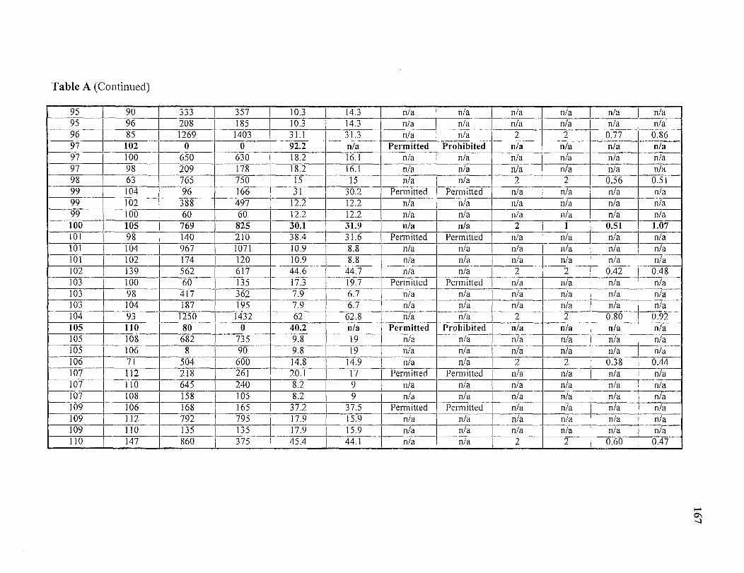
Table A (Continued)
95 90 333 357 10.3 14.3 n/a n/a n/a n/ n/a n/a95 96 208 10LT3 14.3 n/a n/a n/a n/a n/a n/a96 1403 31.I 31.3 n/a n/a 2 2 0.77 0.8697 0 92.2 n/a Permitted Prohibited n/a n/a n/a n/a97 100 650 630 18.2 16.1 n/a n/a n/a n/a n/a n/a97 98 209 178 18LT2 16,1 n/a n/a n/a n/a n/a n/a98 63 765 750 15 15 n/a n/a 2 2 0.56 0LT5199 104 96 166 31 30.2 Permitted Permitted n/a n/a n/a n/a99 102 388 497 12.2 12LT2 n/a n/a n/a n/a n/a n/a99 00 60 60 12.2 122 n/a n/a n/a n/a n/a n/a100 105 769 825 30.1 31.9 n/a n/a 2 1 0.51 1.07101 98 140 210 38LT4 31.6 Permitted n/a n/a n/a n/a101 104 967 1071 10,9 8.8 n/a n/a n/a n/a n/a10 102 174 120 10.9 8.8 n/a n/a n/a nia n/a102 139 562 617 44.6 44,7 n/a 2 2 0.42 0.48103 100 60 135 17.3 19LT7 Permitted n/a n/a n/a n/a103 98 417 362 7.9 6.7 n/a n/a n/a n/a n/a n/a103 lO4 187 195 7.9 6LT7 n/a n/a n/a n/a n/a n/a104 93 1250 1432 62 62.8 n/a n/a 2 2 0,80 0.92105 110 80 0 40.2 n/a Permitted Prohibited n/a n/a n/a n/a105 108 682 735 9.8 19 n/a n/a n/a n/a n/a n/a105 106 8 90 9.8 9 n/a n/a n/a n/a n/a n/a106 71 504 600 14.8 4.9 n/a n/a 2 2 0.38 0.44107 112 218 261 20.I 17 Permitted Permitted n/a n/a n/a n/a107 110 645 240 8LT2 9 n/a n/a n/a n/a n/a n/a107 108 158 105 8.2 9 n/a n/a n/a n/a n/a n/a109 106 168 165 37.2 37.5 Permitted Permitted n/a n/a n/a n/a109 112 792 795 17LT9 15.9 n/a n/a n/a n/a n/a n/a109 110 135 135 17.9 15.9 n/a n/a n/a n/a n/a n/a110 147 860 375 45.4 44LT1 n/a n/a 2 2 0.60 0.47
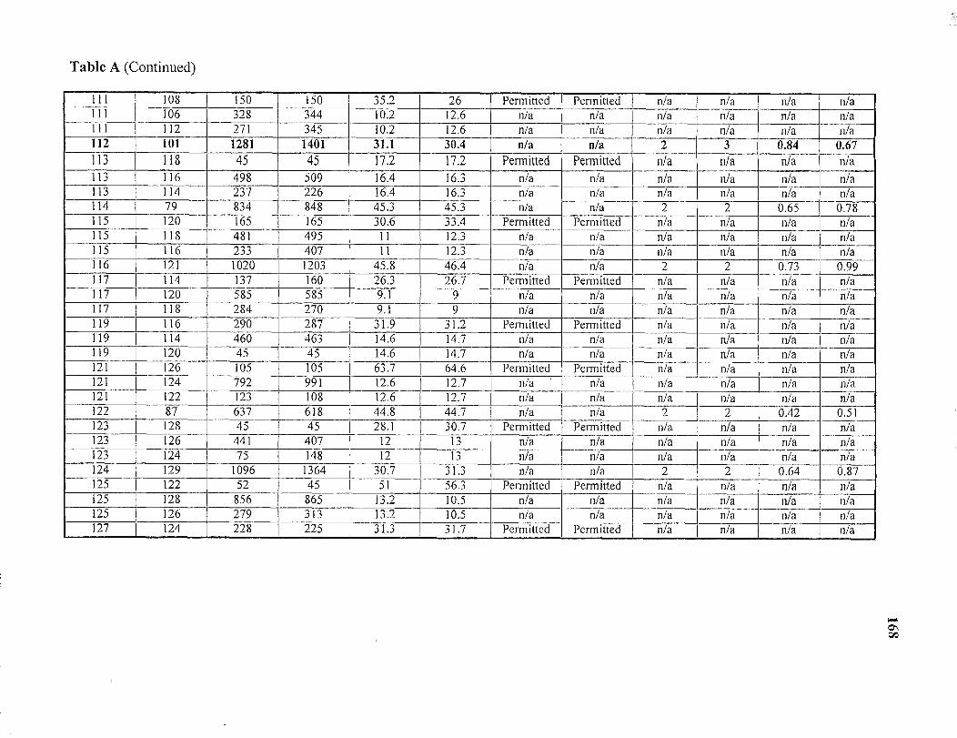
Table A (Continued)
111 108 150 150 35.2 26 Permitted Permitted n/a n/a n/a n/a11 1 106 328 344 10.2 12LT6 n/a n/a n/a n/a n/a n/a111 112 271 345 10.2 12.6 n/a n/a n/a n/a n/a n/a112 101 1281 1401 31.1 30.4 n/a n/a 2 3 0.84 0.671 13 118 45 45 17.2 17.2 Perm itteditted Perm itted n/a n/a n/a n/a113 116 498 509 16.4 16.3 n/a n/a n/a n/a n/a n/a113 114 237 226 16.4 16.3 n/a n/a n/a n/a n/a n/a1 14 79 834 848 45.3 45.3 n/a n/a 2 2 0.65 0.78115 120 165 165 30.6 33.4 Permitted Permitted n/a n/a n/a n/a115 118 481 495 11 12.3 n/a n/a n/a n/a n/a n/a115 116 233 407 11 12.3 n/a n/a n/a n/a n/a n/a116 121 1020 1203 45.8 46.4 n/a n/a 2 2 0.73 0.9911 7 114 137 160 26.3 26,7 Permitted Perm itted n/a n/a n/a n/a117 120 585 585 9.I 9 n/a n/a n/a n/a n/a n/a117 118 284 270 9LT1 9 n/a n/a n/a n/a n/a n/a119 116 290 287 31.9 31.2 Permitted Permitted n/a n/a n/a n/a119 114 460 463 14.6 14.7 n/a n/a n/a n/a n/a n/a119 120 45 45 14.6 14LT7 n/a n/a n/a n/a n/a n/a121 126 105 105 63.7 64.6 Permitted Permitted n/a n/a n/a n/a121 124 792 991 12.6 12.7 n/a n/a n/a n/a n/a n/a121 122 123 108 12LT6 12.7 n/a n/a i /a n/a n/a n/a122 87 637 618 44.8 44.7 n/a n/a 2 2 0.42 0.51123 128 45 45 28.1 30LT7 Permitted Permitted n/a n/a n/a n/a
n/a123 126 441 407 12 13 n/a n/a /a n/a n/a123 124 75 148 12 13 n/a n/a n/a n/a n/a n/a124 129 1096 1364 30.7 31.3 n/a n/a 2 2 0.64 0.87125 122 52 45 51 56.3 Permitted Permitted n/a n/a n/a n/a125 128 856 865 13.2 10.5 n/a n/a n/a n/a n/a n/a125 126 279 313 13.2 10.5 n/a n/a n/a n/a n/a
,n/a
127 124 228 225 31.3 31.7 Permitted Permitted n/a n/a Ilia n/a
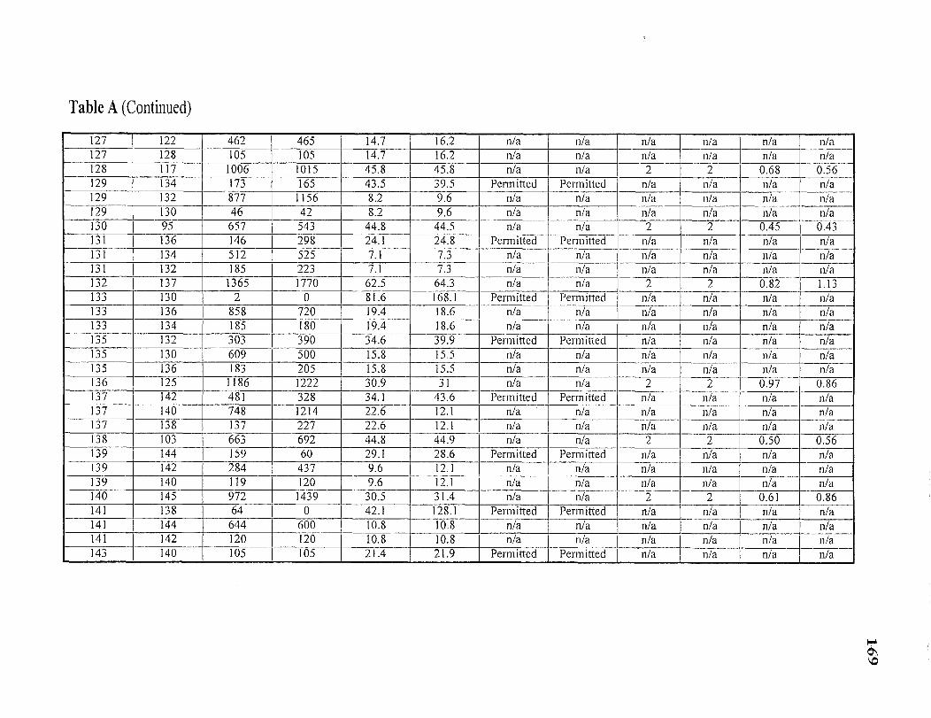
Table A (Continued)
1 27 122 462 465 14.7 16.2 n/a n/a n/a n/a n/a n/a127 128 105 105 14LT7 16.2 n/a n/a n/a n/a n/a n/a128 117 1006 1015 45LT8 45.8 n/a n/a 2 2 0.68 0LT56129 134 173 165 43.5 39.5 Permitted Permitted n/a n/a n/a n/a129 132 877 1156 8.2 9.6 n/a n/a n/a n/a n/a n/a129 130 46 42 8.2 9.6 n/a n/a n/a n/a n/a n/a130 95 657 543 44.8 44.5 n/a n/a 2 2 0.45 0.43131 136 146 298 24.1 24.8 Permitted Permitted n/a n/a n/a n/a1 31 134 512 525 7.I 7.3 n/a n/a n/a n/a n/a n/a131 132 185 223 7.I 7.3 n/a n/a n/a n/a n/a n/a132 137 1365 1770 62.5 64.3 n/a n/a 2 2 0.82 1LT13133 130 2 0 81.6 168.1 Permitted Permitted n/a n/a n/a n/a133 136 858 720 19LT4 18.6 n/a n/a n/a n/a n/a n/a133 134 185 180 19.4 18.6 n/a n/a n/a n/a n/a n/a135 132 303 390 34.6 39.9 Permitted Permitted n/a n/a n/a n/a135 130 609 500 15.8 15.5 n/a n/a n/a n/a n/a i /a135 136 183 205 15.8 15.5 n/a n/a n/a n/a n/a n/a136 125 1186 1222 30.9 31 n/a n/a 2 2 0,97 0.86137 142 481 328 34.I 43.6 Permitted Permitted n/a n/a n/a n/a137 140 748 1214 22LT6 12.I n/a n/a n/a n/a n/a n/a137 138 137 227 22.6 12.1 n/a n/a n/a n/a n/a n/a138 103 663 692 44.8 44.9 n/a n/a 2 2 0.50 0.56139 144 159 60 29LTI 28LT6 Permitted Permitted n/a n/a n/a n/a1 39 142 284 437 9.6 12.I n/a n/a n/a n/a n/a n/a139 140 119 120 9.6 12.I n/a n/a n/a n/a n/a n/a140 145 972 1439 30,5 31.4 n/a n/a 2 2 0.61 0.86141 138 64 0 42.1 128LT1 Permitted Permitted n/a n/a n/a n/a141 144 644 600 10LT8 10.8 n/a n/a n/a n/a n/a n/a141 142 120 120 10.8 10.8 n/a n/a n/a n/a n/a n/a143 140 105 105 21.4 21.9 Permitted Permitted n/a n/a n/a n/a

Table A (Continued)
143 138 463 465 15.7 15.8 n/a n/a n/a n/a n/a n/a143 144 242 240 15.7 15.8 n/a n/a n/a n/a n/a n/a144 133 1044 900 61.2 60.6 n/a n/a 2 2 0.87 0.60145 150 375 705 24.9 65.3 Permitted Permitted n/a n/a n/a n/a145 148 589 705 12.1 14.4 n/a n/a n/a n/a n/a n/a145 146 8 29 12.I 14LT4 n/a n/a n/a n/a n/a n/a146 111 749 839 45.I 45.3 n/a n/a 2 2 0.42 0.53147 152 39 0 33.3 29LT4 Permitted Permitted n/a n/a n/a n/a147 150 510 180 13.8 12.I n/a n/a n/a n/a n/a n/a147 148 311 195 13.8 12.I n/a n/a n/a n/a n/a n/a149 146 253 315 41.8 52,3 Permitted Permitted n/a n/a n/a n/a149 152 512 450 14LT7 15.1 n/a n/a n/a n/a n/a n/a149 150 60 60 14.7 15LT1 n/a n/a n/a n/a n/a n/a151 148 75 75 18.2 14.2 Permitted Permitted n/a n/a n/a n/a151 146 488 495 15.9 14LT8 n/a n/a n/a n/a n/a n/a151 152 277 270 15.9 14LT8 n/a n/a n/a n/a n/a n/a152 141 827 720 30.2 30 n/a n/a 2 2 0.58 0.71
APPENDIX B
SUMMARY OF UTNDP RESULTS OF TEST NETWORK 4UNDER THREE O-D PLANS
171

Table B Summary of UTNDP Results Under Three O-D Plans
Node 0-D Plan 1 (Original) 0-D Plan 2 (50% of Original) O-D Plan 3 (10% of Original)Starting Ending Avg.
FlowAvg.Delay
LeftTurn
No. ofLn.
V/CRatio
Avg.Flow
Avg.Delay
LeftTurn
No. ofLn.
V/CRatio
Avg.Flow
Avg.Delay
LeftTurn
No. ofLn.
V/CRatio
33 38 287 33.6 Prmtd. N/a n/a 125 19.2 Prmtd. N/a n/a 14 11.7 Prmtd. N/a n/a33 36 433 14.3 n/a n/a n/a 235 12.3 n/a n/a n/a 59 11.9 n/a n/a n/a33 34 60 14.3 n/a n/a n/a 30 12.3 n/a n/a n/a 6 11.9 n/a n/a n/a35 40 45 26.5 Prmtd. N/a n/a 23 20.7 Prmtd. N/a n/a 5 17.5 PrmtdLT N/a n/a35 38 315 11.5 n/a n/a n/a 188 10.8 n/a n/a n/a 14 10.8 n/a n/a n/a35 36 420 11.5 n/a n/a n/a 180 10.8 n/a n/a n/a 60 10.8 n/a n/a n/a36 41 1154 46.2 n/a 2 0.85 507 44LT4 n/a 2 0.47 119 43.5 n/a 2 0.1237 34 315 28.5 Prmtd. N/a n/a 135 20.7 Prmtd. N/a n/a 27 15.6 PrmtdLT N/a n/a37 40 510 15.6 n/a n/a n/a 298 10.4 n/a n/a n/a 58 9.5 n/a n/a n/a37 38 45 15LT6 n/a n/a n/a 89 10.4 n/a n/a n/a 28 9LT5 n/a n/a n/a38 75 647 14LT9 n/a 2 0.51 401 14LT7 n/a 2 0,33 55 14.4 n/a 2 0.0539 36 301 33.9 Prmtd. N/a n/a 92 20LTI Prmtd. N/a n/a 0 18.2 Prmtd. N/a n/a39 34 450 13.4 n/a n/a n/a 248 11.1 n/a n/a n/a 50 11.4 n/a n/a n/a39 40 270 13.4 n/a n/a n/a 92 11.1 n/a n/a n/a 20 11.4 n/a n/a n/a41 46 133 27 Prmtd. N/a n/a 91 12.5 Prmtd. N/a n/a 11 9.7 Prmtd. N/a n/a41 44 916 7.4 n/a n/a n/a 364 5.8 n/a n/a n/a 98 5.8 n/a n/a n/a41 42 105 7.4 n/a n/a n/a 53 5.8 n/a n/a n/a 11 5.8 n/a n/a n/a43 48 90 28.4 Prmtd. N/a n/a 112 19LT3 Prmtd. N/a n/a 23 11.7 Prmtd. N/a n/a43 46 360 16.6 n/a n/a n/a 135 12.5 n/a n/a n/a 5 11.8 n/a n/a n/a43 44 300 16.6 n/a n/a n/a 128 12LT5 n/a n/a n/a 48 11.8 n/a n/a n/a44 49 1335 31.2 n/a 2 0.84 673 29.9 n/a 2 0.53 213 29LT1 n/a 2 0,1645 42 225 38.4 Prmtd. N/a n/a 125 17.9 Prmtd. N/a n/a 23 11.7 PrmtdLT N/a n/a45 48 690 14.1 n/a n/a n/a 387 8 n/a n/a n/a 80 6.9 n/a n/a n/a45 46 45 14.1 n/a n/a n/a 0 8 n/a n/a n/a 0 6.9 n/a n/a n/a46 83 538 14.8 n/a 2 0.38 226 14.6 n/a 2 0.23 15 14.4 n/a 2 0.0547 44 120 35.3 PrmtdLT N/a n/a 182 12.3 PrmtdLT N/a n/a 68 6.7 Prmtd. N/a nia47 42 510 5.7 n/a n/a n/a 243 6.8 n/a n/a n/a 50 6.1 n/a n/a n/a

Table B (Continued)
47 48 90 5.7 n/a n/a n/a 23 6.8 n/a n/a n/a 11 6.1 n/a n/a n/a
48 37 870 45.4 n/a 2 0.55 522 44.5 n/a 2 0.31 113 43LT5 n/a 2 0.11
49 54 150 37.5 Prmtd. N/a n/a 0 n/a Prhted. N/a 68 11.1 Prmtd. N/a n/a
49 52 1035 10,1 n/a n/a 531 10.1 n/a n/a 110 6.7 n/a n/a n/a
49 50 150 10.1 n/a n/a 143 10.I n/a n/a 36 6LT7 n/a n/a n/a
51 56 195 30.3 Prmtd. N/a n/a 98 15.5 Prmtd. N/a 28 11.3 Prmtd. N/a n/a
51 54 n/a n/a 368 13.2 n/a n/a 56 11.5 n/a n/a n/a
51 52 287 17.4 n/a n/a 120 13.2 n/a n/a 33 11.5 n/a n/a n/a
52 57 2 I.10 651 59.7 n/a 2 0.48 143 58 n/a 2 0.11
53 50 150 92.I Prmtd. N/a n/a 75 35LT7 Prmtd. N/a 15 19.7 Prmtd. N/a n/a53 56 705 10 n/a n/a 384 14.1 n/a n/a 74 11,5 n/a n/a n/a
53 54 263 10 n/a n/a 183 14.1 n/a n/a 73 11.5 n/a n/a n/a54 91 1101 2 0.73 550 14.8 n/a 2 0.42 196 14.6 n/a 2 0.15
55 52 180 44.3 Pnntd. N/a n/a 0 26 Prmtd. N/a n/a 0 18.6 Prmtd. N/a n/a55 50 510 n/a n/a 188 12.2 n/a n/a n/a 30 11.4 n/a n/a n/a55 56 n/a n/a 30 12.2 n/a n/a n/a 0 11LT4 n/a n/a n/a56 45 960 30.4 n/a 2 0.65 512 29.6 n/a 2 0.37 103 29 n/a 2 0.0657 62 212 38LT6 PrmtdLT N/a n/a 99 18.5 Prmtd. N/a n/a 0 16 Prmtd. N/a n/a57 60 1095 8.4 n/a n/a n/a 434 8.2 n/a n/a n/a 110 9.4 n/a n/a n/a57 58 196 8.4 n/a n/a n/a 117 8.2 n/a n/a n/a 33 9.4 n/a n/a n/a59 64 254 40.9 PrmtdLT N/a n/a 189 20.4 Prmtd. N/a n/a 48 12.8 Prmtd, N/a n/a59 62 451 18LT8 n/a n/a n/a 164 12.3 n/a n/a n/a 5 12.6 n/a n/a n/a59 60 120 18.8 n/a n/a n/a 60 12.3 n/a n/a 1 /a 30 12.6 n/a n/a n/a60 65 1336 31.2 n/a 2 0.64 703 30 n/a 2 0LT50 191 29.1 n/a 2 0.12
61 58 105 38.2 Prmtd. N/a n/a 107 12.8 PrmtdLT N/a n/a 20 7.2 Prmtd. N/a n/a61 64 804 3.9 n/a n/a n/a 424 5.6 n/a n/a n/a 105 4.2 n/a n/a n/a61 62 60 3.9 n/a n/a n/a 39 5LT6 n/a n/a n/a 12 4LT2 n/a n/a n/a62 99 723 15 n/a 2 0.59 302 14.6 n/a 2 0.31 17 14LT4 n/a 2 0LT0563 60 121 28.3 Prmtd. N/a n/a 208 10.2 Prmtd. N/a n/a 51 7 Prmtd. N/a n/a63 58 569 10.5 n/a n/a n/a 211 6.7 n/a n/a n/a 34 7 n/a n/a n/a

Table B (Continued)
• 10.5 9 7 n/a n/a n/a61.5 162 58LTI n/a 2 0LT11
65 70 0 n/a n/a 6 Prmtd N/a n/a65 68 750 12.3 3.6 n/a n/a n/a65 66 586 12.3 328 3.6 n/a n/a n/a67 72 310 28.I • N/a n/a 153 13.8 Prmtd. N/a n/a67 70 440 14.3 n/a n/a 222 13.4 n/a n/a n/a67 68 60 14LT3 n/a 30 12.2 n/a n/a n/a 6 13.4 n/a 1 /a n/aG9 66 45 19.9 n/a 15.2 Prmtd. N/a n/a69 72 613 15.7 n/a 9LTI n/a n/a n/a69 70 167 15.7 n/a 9.1 n/a n/a n/a70 107 G06 14.9 0.43 328 14.5 n/a 2 0.0871 68 225 n/a 113 23 13.3 Prmtd. N/a n/a71 66 330 18.6 n/a 130 21 8.3 n/a n/a n/a71 72 45 18.6 n/a 133 7.4 18 8.3 n/a n/a n/a72 61 969 30.5 n/a 2 0.47 137 29 n/a 2 0.0973 78 345 39.9 Prmtd. n/a 19 11LT2 Prmtd, N/a n/a73 76 481 i n/a 342 n/a 72 11.4 n/a n/a n/a73 74 224 15.3 n/a 68 n/a 14 11.4 n/a n/a n/a74 39 1021 15.3 n/a 1 14.7 0.32 69 14,5 n/a 2 0.0675 80 90 16.2 Prmtd. n/a 14 8.5 PrmtdLT N/a n/a75 78 437 6.6 n/a n/a 41 5.3 n/a n/a n/a75 76 120 6.6 n/a n/a n/a 0 5.3 n/a n/a n/a76 81 808 45LT2 n/a 0LT64 432 44.2 2 0LT40 72 43.4 n/a 2 0LT0677 74 290 22.9 Prmtd. n/a 182 13.5 PrmtdLT n/a 38 8LT3 Pm d N/a n/a77 80 540 7.3 n/a n/a 270 5.3 n/a n/a 54 5 n/a n/a n/a77 78 285 7.3 n/a n/a 121 5.3 n/a n/a 43 5 n/a n/a n/a78 115 1067 46 n/a 2 0.78 480 44LT4 n/a 2 0.34 103 43.4 n/a 0.0979 76 207 26LT8 Prmtd. N/a n/a 0 28.1 Prmtd. n/a 0 25.2 Prmtd n/a79 74 506 9.3 n/a n/a n/a 182 14LT8 n/a n/a n/a 8 15.6 n/a n/a n/a
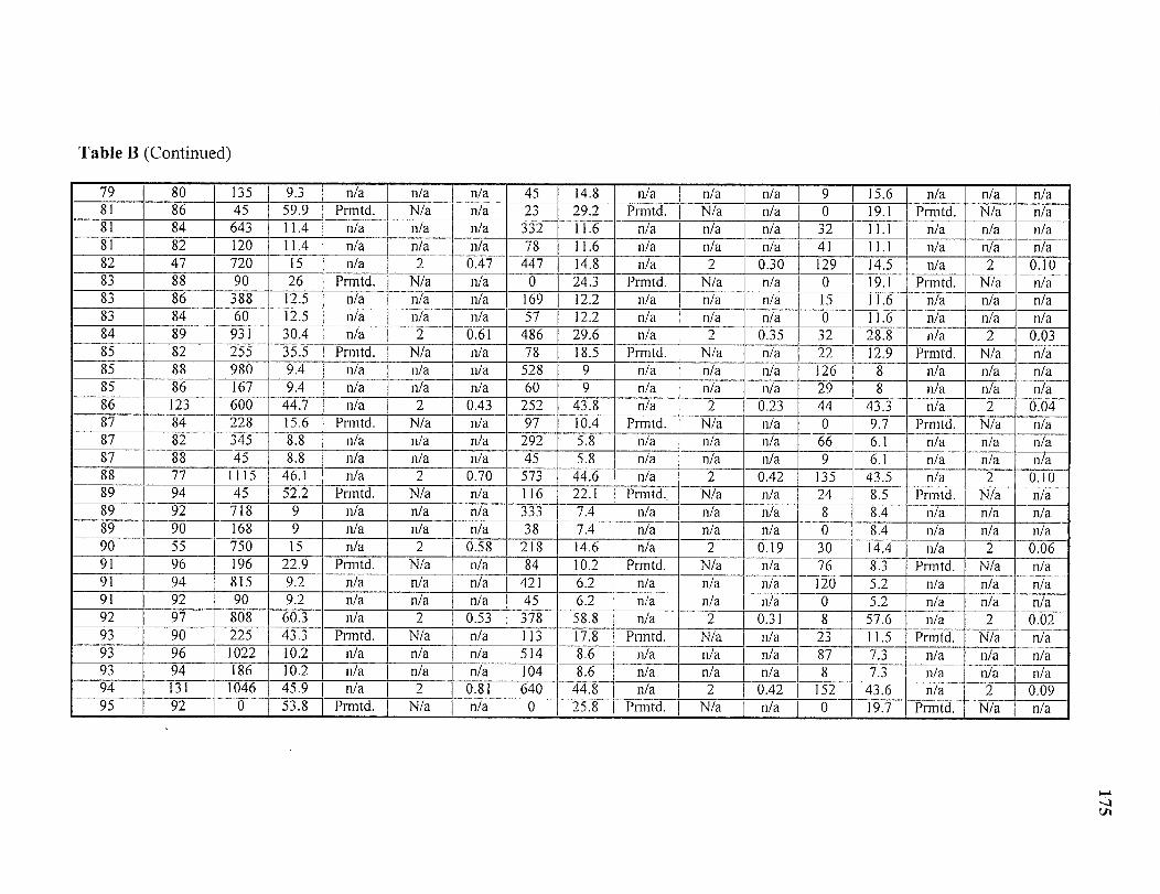
Table B (Continued)
79 80 135 9LT3 n/a n/a n/a 45 14.8 n/a n/a n/a 9 15.6 n/a n/a n/a81 86 45 59.9 Prmtd. N/a 23 29.2 Prmtd. N/a n/a 0 19.I Prmtd. N/a n/a81 84 643 11.4 n/a n/a 332 11.6 n/a n/a n/a 32 11.1 n/a n/a n/a81 82 120 11LT4 n/a n/a n/a 78 11.6 n/a n/a n/a 41 11.1 n/a n/a n/a82 47 720 15 n/a 2 0.47 447 14.8 n/a 2 0.30 129 14.5 n/a 2 0.1083 88 90 26 Prmtd. N/a 0 24.3 Prmtd. N/a n/a 0 19.1 Prmtd. N/a n/a83 86 388 12.5 n/a n/a n/a 169 12.2 n/a n/a n/a 15 11.6 n/a n/a n/a83 84 60 12.5 n/a n/a n/a 57 12.2 n/a n/a n/a 0 11.6 n/a n/a n/a84 89 931 30.4 n/a 2 0.61 486 29.6 n/a 2 0.35 32 28.8 n/a 2 0.0385 82 255 35.5 Prmtd. N/a n/a 78 18.5 Prmtd. N/a n/a 22 12LT9 Prmtd. N/a n/a85 88 980 9.4 n/a n/a n/a 528 9 n/a n/a n/a 126 8 n/a n/a n/a85 86 167 9.4 n/a n/a n/a 60 9 n/a n/a n/a 29 8 n/a n/a n/a86 123 600 44.7 n/a 2 0.43 252 43.8 n/a 2 0.23 44 43.3 n/a 2 0LT0487 84 228 15.6 Prmtd N/a n/a 97 10.4 Prmtd. N/a n/a 0 9.7 Prmtd. N/a n/a87 82 345 8.8 n/a n/a n/a 292 5.8 n/a n/a n/a 66 6.1 n/a n/a n/a87 88 45 8.8 n/a n/a n/a 45 5LT8 n/a 9 6.1 n/a n/a n/a88 77 1115 46.I n/a 2 0.70 573 44.6 n/a 2 0.42 135 43LT5 n/a 2 0LTI089 94 45 52.2 Pnntd. N/a n/a 116 22.1 Prmtd. n/a 24 8.5 Prmtd. N/a n/a89 92 718 9 n/a n/a n/a 333 7.4 n/a n/a 8 8LT4 n/a n/a n/a89 90 168 9 n/a n/a n/a 38 7.4 n/a 0 8LT4 n/a n/a n/a90 55 750 15 n/a 2 0LT58 218 14.6 n/a 2 0.19 30 14.4 n/a 2 0.0691 96 196 22.9 PrmtdLT N/a n/a 84 10.2 Prmtd. 76 8.3 Prmtd. N/a n/a91 94 815 9.2 n/a n/a n/a 421 6.2 n/a 120 5.2 n/a n/a n/a91 92 90 9.2 n/a n/a n/a 45 6.2 n/a 0 5.2 n/a n/a n/a92 97 808 60LT3 n/a 2 0.53 378 58.8 n/a 2 0.31 8 57.6 n/a 2 0.0293 90 225 43LT3 Prmtd. N/a n/a 113 17.8 Prmtd. N/a 23 11.5 Prmtd. N/a n/a93 96 1022 10.2 n/a n/a n/a 514 8.6 n/a 87 7.3 n/a n/a n/a93 94 186 10.2 n/a n/a n/a 104 8.6 n/a 8 7.3 n/a n/a n/a94 131 1046 45.9 n/a 2 0.81 640 44.8 n/a 2 0.42 152 43.6 n/a 2 0.0995 92 0 53.8 Prmtd. N/a n/a 0 25.8 Prmtd. N/a n/a 0 19.7 Prmtd. N/a n/a

Table B (Continued)
95 90 357 14.3 n/a n/a n/a 68 11.5 n/a n/a n/a 8 11.5 n/a n/a n/a95 96 185 14.3 n/a n/a n/a 68 11.5 n/a n/a n/a 14 11.5 n/a n/a n/a96 85 1403 31.3 n/a 2 0.86 666 29.9 n/a 2 0.42 176 29.I n/a 2 0.1097 102 0 Prhted. 38 Prmtd. N/a n/a 0 23.7 PrmtdLT N/a n/a97 100 630 16.I n/a 15.3 n/a n/a n/a 8 14LT5 n/a n/a n/a97 98 178 16.I n/a 15.3 n/a n/a n/a 0 14.5 n/a n/a n/a98 63 750 15 n/a 2 0.51 449 14.8 n/a 2 0LT32 94 14.5 n/a 2 0.0599 104 166 30.2 Prmtd. 51 22.3 Prmtd. N/a n/a 0 18.6 PrmtdLT N/a n/a99 102 497 12.2 n/a 205 10.5 n/a n/a n/a 17 11 n/a n/a n/a99 100 60 12LT2 n/a 47 10.5 n/a n/a n/a 0 11 n/a n/a n/a100 105 825 31.9 n/a 1 1.07 430 29.5 n/a 2 0.28 41 28.9 n/a 2 0.02101 98 210 31.6 Prmtd. n/a 20 19.3 Prmtd. N/a n/a 0 13.7 Prmtd. N/a n/a101 104 1071 8.8 n/a 9.5 n/a n/a n/a 56 8.7 n/a n/a n/a101 102 120 8.8 n/a 9LT5 n/a n/a n/a 6 8LT7 n/a n/a n/a1 02 139 617 44,7 n/a 2 0.48 255 43.8 n/a 2 0.21 23 43.3 n/a 2 0.03103 100 135 19.7 Prmtd. 68 12.I Prmtd. N/a n/a 33 8.3 Prmtd. N/a n/a103 98 362 6.7 n/a 6.6 n/a n/a n/a 94 5.2 n/a n/a n/a103 104 195 6LT7 n/a 165 6LT6 n/a n/a n/a 60 5.2 n/a n/a n/a104 93 1432 62.8 n/a 2 0.92 730 60 n/a 2 0.53 117 58 n/a 2 0.11105 110 0 n/a Prhted. n/a 38 19 Prmtd. N/a n/a 0 14.I Prmtd. N/a n/a105 108 735 19 n/a 368 9 n/a n/a n/a 41 8.6 n/a n/a n/a105 106 90 19 n/a 9 n/a n/a n/a 0 8LT6 n/a n/a n/a106 71 600 14.9 n/a 2 0.44 376 14.7 n/a 2 0.32 62 14.4 n/a 2 0.04107 112 261 17 Prmtd. 10.9 Prmtd. N/a n/a 0 11.4 Prmtd. N/a n/a107 110 240 9 n/a 7 n/a n/a n/a 36 7.I n/a n/a n/a107 108 105 9 n/a n/a 53 7 n/a n/a n/a 44 7.I n/a n/a n/a109 106 165 37.5 Prmtd. n/a 128 19 Prmtd. N/a n/a 34 11LT4 Prmtd. N/a n/a109 112 795 15.9 n/a n/a 352 13 n/a n/a n/a 62 11.4 n/a n/a n/a109 110 135 15.9 n/a n/a 68 13 n/a n/a n/a 14 11.4 n/a n/a n/a110 147 375 44.I n/a 2 0.47 225 43.7 n/a 2 0.21 50 43.3 n/a 2 0LT05
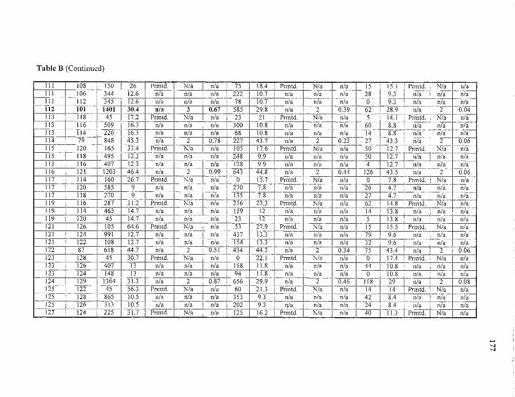
Table B (Continued)
111 108 150 26 PrmtdLT N/a n/a 75 18.4 Prmtd. N/a n/a 15 15.1 Prmtd. N/a n/a111 106 344 12.6 n/a n/a n/a 222 10LT7 n/a n/a 28 9.3 n/a n/a n/a111 112 345 12LT6 n/a n/a n/a 78 10.7 n/a n/a 0 9.3 n/a n/a n/a112 101 1401 30.4 n/a 3 0.67 585 29.8 n/a 2 0.39 62 28,9 n/a 2 0.04113 118 45 17.2 Prmtd. N/a n/a 23 21 Prmtd. N/a n/a 5 14.1 Prmtd. N/a n/a113 116 509 16.3 n/a n/a n/a 300 10.8 n/a n/a n/a 60 8.8 n/a n/a n/a113 114 226 16,3 n/a n/a n/a 68 10.8 n/a n/a n/a 14 8.8 n/a n/a n/a114 79 848 45.3 n/a 2 0.78 227 43LT7 n/a 2 0.23 27 43.3 n/a 2 0.061 15 120 165 33.4 PrmtdLT N/a n/a 105 17.6 Prmtd. N/a 1 /a 50 12.7 Prmtd. N/a n/a115 118 495 12.3 n/a n/a n/a 248 9.9 n/a n/a n/a 50 12.7 n/a n/a n/a115 116 407 12.3 n/a n/a n/a 128 9.9 n/a n/a n/a 4 12.7 n/a n/a n/a116 121 1203 46.4 n/a 2 0.99 643 44.8 n/a 2 0.44 126 43.5 n/a 2 0.06117 114 160 26.7 PrmtdLT N/a n/a 0 15.7 Prmtd. N/a n/a 0 7.8 Prmtd. N/a n/a117 120 585 9 n/a n/a n/a 270 7.8 n/a n/a n/a 26 4.7 n/a n/a n/a117 118 270 9 n/a n/a n/a 135 7.8 n/a 27 4.7 n/a n/a n/a119 116 287 31.2 Prmtd. N/a n/a 216
15923
22.3 Prmtd.12 n/a
12 n/a n/a
n/an/an/a
6214
14.8 PrmtdLT N/a n/a119119
114120
46345
14.714.7
n/an/a
n/an/a
n/an/a
13.8 n/a n/a n/a5 13.8 n/a n/a n/a
1 21 126 105 64.6 Prmtd. N/a n/a 53 27.9 Prmtd. N/a n/a 15 15.5 Prmtd. N/a n/a121 124 991 2.7 n/a n/a n/a 437 13,3 n/a n/a 79 9.6 n/a n/a n/a121 122 108 12,7 n/a n/a 154 13.3 n/a n/a n/a 32 9.6 n/a n/a n/a1 22 87 618 44.7 n/a 2 0.51 434 44.2 n/a 2 0.34 75 43.4 n/a 2 0.06123 128 45 30.7 Prmtd. N/a n/a 0 22.I Prmtd. N/a n/a 0 17.4 Prmtd. N/a n/a123 126 407 13 n/a n/a n/a 158 11.8 n/a n/a n/a 44 10.8 n/a n/a n/a123 124 148 13 n/a n/a n/a 94 11.8 n/a n/a 0 10.8 n/a n/a n/a124 129 1364 31LT3 n/a 2 0.87 656 29.9 n/a 2 0.46 118 29 n/a 2 0.08125 122 45 56.3 Prmtd. N/a n/a 60 21.3 PrmtdLT N/a n/a 14 14 Prmtd. N/a 11/a125 128 865 10.5 n/a n/a n/a 353 9.3 n/a n/a n/a 42 8.4 n/a n/a n/a125 126 313 10.5 n/a n/a n/a 202 9.3 n/a n/a n/a 24 8.4 n/a n/a n/a127 124 225 31.7 Prmtd. N/a n/a 125 16LT2 PrmtdLT N/a n/a 40 11.3 Prmtd. N/a n/a
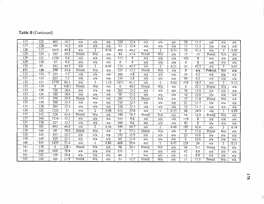
Table B (Continued)
127 122 465 16.2 n/a n/a n/a 220 12LT4 n/a n/a n/a 29 11LT2 n/a n/a n/a127 128 105 16.2 n/a n/a 12LT4 n/a n/a n/a 11 11.2 n/a n/a n/a128 117 1015 45.8 n/a 2 0.56 405 44.2 n/a 2 0.31 53 43,3 n/a 2 0.05129 134 165 39.5 Prmtd. N/a 17.4 Prmtd. N/a n/a 17 13 PrmtdLT N/a n/a129 132 1156 9.6 n/a n/a n/a 572 9 n/a n/a n/a 102 8 n/a n/a n/a129 130 42 9.6 n/a n/a n/a 0 9 n/a n/a n/a 0 8 n/a n/a n/a130 95 543 44.5 n/a 2 0LT43 135 43LT5 n/a 2 0.21 21 43.2 n/a 2 0LT01131 136 298 24.8 Prmtd. N/a 225 12.2 PrmtdLT N/a n/a 0 n/a Prh ed. N/a n/a131 134 525 7.3 n/a n/a 5.8 n/a n/a n/a 53 6.3 n/a n/a n/a131 132 223 7.3 n/a n/a 5.8 n/a n/a n/a 99 6LT3 n/a n/a n/a132 137 1770 64.3 n/a 2 I.13 1011 61.I n/a 2 0.66 258 58.4 n/a 2 0LT13133 130 0 168.I PrmtdLT N/a n/a 0 40.4 Prmtd. N/a n/a 0 23.I Prmtd. N/a n/a133 136 720 18.6 n/a n/a 15.2 n/a n/a n/a 48 13.6 n/a n/a n/a133 134 180 18.6 n/a n/a 90 15.2 n/a n/a n/a 18 13.6 n/a n/a n/a135 132 390 39.9 Prmtd. N/a 285 23LT6 Prmtd. N/a n/a 57 11.8 Prmtd_ N/a n/a135 130 500 15.5 n/a n/a 12.3 n/a n/a n/a 21 11.7 n/a n/a n/a135 136 205 15.5 n/a n/a 12.3 n/a n/a n/a 32 11.7 n/a n/a n/a136 125 1222 31 n/a 2 0.86 615 29.8 n/a 2 0.53 80 28.9 n/a 2 0.09137 142 328 43.6 Prmtd. N/a 188 19.7 Prmtd. N/a n/a 54 12.9 Prmtd. N/a n/a137 140 1214 12.1 n/a n/a 555 9LT6 n/a n/a n/a 119 8 n/a n/a n/a137 138 227 12.I n/a n/a 9.6 n/a n/a n/a 85 8 n/a n/a n/a138 103 692 44.9 n/a 2 0LT56 599 44.7 n/a 2 0LT49 187 43LT6 n/a 2 0.16139 144 60 28.6 Prmtd. N/a 22.3 PrmtdLT N/a 0 17.6 Prmtd. N/a n/a139 142 437 12.1 n/a n/a n/a 195 11.9 n/a n/a 23 10.8 n/a n/a n/a139 140 120 12.1 n/a n/a n/a 60 11.9 n/a n/a 0 10LT8 n/a n/a n/a140 145 1439 31LT4 n/a 2 0.86 668 29.9 n/a 2 0LT47 129 29 n/a 2 0.11141 138 0 128.I Prmtd. N/a 20.3 PrmtdLT N/a n/a 56 9.I Prmtd, N/a n/a141 144 600 10.8 n/a n/a nia 233 7 n/a n/a n/a 42 8.9 n/a n/a n/a141 142 120 10LT8 n/a n/a n/a 60 7 n/a n/a n/a 12 8.9 n/a n/a n/a143 140 105 21LT9 Prmtd, N/a n/a 53 12LT2 Prmtd. N/a n/a 11 11LT5 PrmtdLT N/a n/a

Table B (Continued)
143 138 465 15LT8 n/a n/a n/a 233 13 n/a n/a n/a 47 11.6 n/a n/a n/a143 144 240 15.8 n/a n/a n/a 120 13 n/a n/a n/a 24 11.6 n/a n/a n/a144 133 900 60.6 n/a 2 0.60 353 58.7 n/a 2 0.45 66 57.8 n/a 2 0.18145 150 705 65.3 PrmtdLT n/a n/a 315 16.8 Prmtd. n/a n/a 65 8,1 Prmtd n/a n/a145 148 705 14.4 n/a n/a n/a 353 9.6 n/a n/a n/a 65 7LT8 n/a n/a n/a145 146 29 14.4 n/a n/a n/a 0 9.6 n/a n/a n/a 0 7.8 n/a n/a n/a146 111 839 45.3 n/a 2 0.53 375 44.I n/a 2 0.21 43 43LT3 n/a 2 0.02147 152 0 29.4 Prmtd. n/a n/a 0 22.4 Prmtd n/a n/a 0 18.I PrmtdLT n/a n/a147 150 180 12.I n/a n/a n/a 128 11.8 n/a n/a n/a 24 11.3 n/a n/a n/a147 148 195 12.I n/a n/a n/a 98 11.8 n/a n/a n/a 26 11LT3 n/a n/a n/a149 146 315 52LT3 Prmtd. n/a n/a 128 19.4 Prmtd. n/a n/a 22 11LT5 PrmtdLT n/a n/a149 152 450 15.1 n/a n/a n/a 255 12.3 n/a n/a n/a 54 11.6 n/a n/a n/a149 150 60 15.1 n/a n/a n/a 30 12.3 n/a n/a n/a 6 11.6 n/a n/a n/a151 148 75 14.2 PrmtdLT n/a n/a 38 11.6 Prmtd. n/a n/a 8 11LT5 Prmtd. n/a n/a151 146 495 14.8 n/a n/a n/a 248 12.8 n/a n/a n/a 21 11.7 n/a n/a n/a151 152 270 14.8 n/a n/a n/a 135 1.2.8 n/a n/a n/a 56 11.7 n/a n/a n/a152 141 720 30 n/a 2 0.71 390 29.4 n/a 2 0.30 110 29 n/a 2 0.09
REFERENCES
1. LeBlanc, L.J. "An Algorithm for the Discrete Network Design Problem."Transportation Science 9(3) (1975q): 183-199.
2. LeBlanc, L. J., Morlok, E. K., and Pierskalla, W. P. "An Efficient Approach toSolving the Road Network Equilibrium Traffic Assignment Problem." Trans.
Res. 9 (1975b): 309-318.
3. Mouskos, K. C. A Tabu-Based Heuristic Search Strategy to Solve a DiscreteTransportation Equilibrium Network Design Problem. 1991. Ph.D Thesis TheUniversity of Texas at Austin.
4. LeBlanc, L. J. and Boyce, D. E. "A Bilevel Programming Algorithm for ExactSolution of the Network Design Problem with User-Optima Flows."Transportation Research B, vol. 20B, No.3 (1986): 259-265.
5. Sheffi, Y. Urban Transportation Networks. 1985. Prentice-Hall, Englewood Cliffs,New Jersey.
6. Abdulaal M., and LeBlanc, L. J. "Continuous Equilibrium Network Design Models."Transportation Research B, Vol. 13B (1979): 19-32.
7. Frank, M., and Wolfe, P. "An Algorithm for Quadratic Programming." NavalResearch Logistics Quarterly 3(1-2) (1956): 95-110.
8. Friesz, T. L. "Transportation Network Equilibrium, Design and Aggregation: KeyDevelopments and Research Opportunities." Transportation Research A, vol.
19A, NoLT5/6 (1985): 413-427.
9. Friesz, T. L., Cho, H. J., Mehta, N. J., Tobin R. L. and Anandalingam, G. "Asimulated annealing approach to the Network Design Problem with VariationalInequality Constraints." Transportation Science, Vol. 26, No. 1(1992).
10. Wardrop, J. G. "Some Theoretical Aspects of Road Traffic Research." Proc. Inst.Civ. Eng., 1, part 11 (1952): 325-378.
11. Webster, F. V. "Traffic Signal Settings." Road Research Technical Paper 39 (1958).Road Research Laboratory, Her Majesty's Stationary Office, London.
12. Beckerman, M. J., McGure, C. B., and Winston, C. B. Studies in the Economics ofTransportation. 1956. Yale University Press, New Haven, Conn.
180
181
13. Berka, S., Boyce, D. E., Raj, J., Ran, B., Tarko, A., and Zhang, Y. "A large-scaleroute choice model with realistic link delay functions for generating highwaytravel times." A technical report in support of the ADVANCE project to IllinoisDepartment of Transportation. 1994.
14. Magnanti, T. L. and Wong, R. T. "Network design and transportation planning:Models and Algorithms." Transportation Science 18 (4) (1984): 362-384.
15. Mahmassani, H. S. and Mouskos, K. C. "Some Numerical Results on theDiagonalization Algorithm for Network Assignment with AsymmetricInteractions Between Cars and Trucks." Transportation Research 22B (1988),275-290.
16. Dionne, R. And Florian, M. "Exact and approximate algorithms for optimal networkdesign." Networks 9 (1979): 37-60.
17. Fisk C. S. "Game Theory and Transportation Systems Modeling." TransportationResearch, 18B (1984), 301-313.
18. Heydecker B. G. And Khoo T. K. "The Equilibrium Network Design Problem."Proceedings of AIRO '90 Conference on Models and Methods for DecisionSupport, Sorrento (1990), 587-602.
19. Hoang, H. H. "A Computational Approach to the Selection of an Optimal Network."Management Science 19 (1973): 488-498.
20. Marcotte P. "Network Optimization with Continuous Control Parameters."Transportation Scicence 17 (1983), 181-197.
21. Bard J. "An Efficient Point Algorithm for a Linear Two-stage OptimizationProblem." Operations Research,31 (1983): 670-684.
22. Bertsekas D. P. and Gafni E. M. "Projection Methods for Variational Inequalitieswith Application to the Traffic Assignment Problem." MathematicalProgramming Studies 17(1982): 139-159.
23. Dafermos S. C. "Traffic Equilibria and Variational Inequality." TransportationScience, 14(1) (1980): 42-54.
24. Glover, F. "Future Paths for Integer Programming and Links to ArtificialIntelligence." Computers and Operations Research, Vol. 13, No. 5 (1986):533-549.
25. Glover, F. "Tabu Search-Part I." ORSA J. Comput. 1(1989): 190-206.
26. Glover, F. "Tabu Search-Part II." ORSA Comput 2 (1990): 4-32.

27. Glover, F. and McMillan, C. "The general employee scheduling problem: Anintegration of MS and Al." Comput. and Opns. Res., Vol. 13. No. 5 (1990).533-549.
28. Jayakrishnan, R., Wei K. T., Prashker, J. N., and Rajadhyaksha, S. "Faster Path-Based Algorithm for Traffic Assignment." Transportation Research Record 1443(1992).
29. Kirkpatrick, S., Gelatt, C. D. and Vecchi, M. P. "Optimization by SimulatedAnnealing." Science 220 (1983): 671-680.
30. Matsuo, H., Suh, C. J., and Sullivan, R. S. "A Controlled Search Simulated AnnealingMethod for the Single Machine Weighted Tardiness Problem." Working Paper87-12-2. 1987. Department of Management, University of Texas at Austin.
31. Meneguzzer, C., Boyce, D. E., Rouphail, N., and Sen, A. Implementation andEvaluation of an Asymmetric Equilibrium Route Choice Model IncorporatingIntersection-Related Travel Times, Report to Illinois Department ofTransportation, Urban Transportation Center, University of Illinois,Chicago,Illinois, 1990.
32. Metropolis, N., Rosenbluth, A., Rosenbluth, M., Teller, A. and Teller, E. "Equationof state calculation by fast computing machines." Journal of Chemical Physics21 (1953): 1087-1092.
33. Smith M. J. "Traffic Signals in Assignment." Transportation Research, 19B (1985),155-160.
34. Allsop R. E. "Some Possibilities for Using Traffic Control to Influence TripDestinations and Route Choice." Proceedings of the Sixth International
Symposium on transportation and Traffic Theory, Sydney, Australia (1974),345-374.
35. Cantarella G. E., Improta G. And Sforza A. "Iterative Procedure for EquilibriumNetwork Traffic Signal Setting." Transportation Research, 25A (1991), 241-249.
36. Chang, E. C. P., and Messer C. J. PASSER 11-90 Program User's Guide. 1991. TexasTransportation Institute, Texas A&M University System, College Station, Texas77843.
37. Dickson T. J. "A Note on Traffic Assignment and Signal Timings in A SignalControlled Road Network." Transportation Research, 15B (1981), 267-271.
38. Garter N. H., Gershwin S. W., Little J. D. C. and Ross P. "Pilot Study of Computer-Based Urban Traffic Management." Transportation Research, 14 B (1980),
182
183
203-217.
39. TRANSYT-7F User's Manual. 1988. Transportation Research Center, University ofFlorida.
40. Yang, H. and Yagar S. "Traffic Assignment and Signal Control in Saturated RoadNetworks." Transportation Research 29A (1995), 125-139.
41. Ziliaskopoulos , A. K. And Mahmassani, H.S. 1996. "On Finding the Least TimePaths Considering Delays for Intersection Movements." TransportationResearch 30B (1996), 359-367.
42. Rouphail, N.M., A. Tarko and C. Li "Signalized Intersections," Draft Chapter 9 ofTraffic Flow Theory Monograph, January 1996.
43. Akcelik, R., "Traffic Signals: Capacity and Timing Analysis", ARRB ResearchReport 123,Australian Road Research Board, Victoria, Australia, March 1981.
44. Reilly, W., et al., "Capacity of Signalized Intersections," Final Report, NCHRPProject 3-28(2), JHK&Associates, Tucson, AZ, 1983.
45. Roess, R., and McShane, W., "Final Report on the New Highway Capacity Manual,"Final Report, NCHRP Project 3-28(B), Transportation Training and ResearchCenter, Polytechnic University, Brooklyn, NY, October 1986.
46. Highway Capacity Manual, Special Report 209, 31' edition, Transportation ResearchBoard, National Research Council, Washington, DC, 1997.
47. Little, J.D.C. "The Synchronization of Traffic Signals by Mixed-Integer LinearProgramming", Operation Research 14 (1966).
48. Marrus,B.S., and Main M.F. "New Method Improves Traffic Signal Timing", TrafficEngineering, 23-26 (1964).
49. "SIGOP: Traffic Signal Optimization Program-A Computer Program to CalculateOptimum Coordination in a Grid Network of Synchronized Traffic Signals,"Traffic Research Corporation, New York, 1966.
50. Gartner, N.H., Little J.D.C., and Gabbay H., "Optimization of Traffic Signal Settingsby Mixed-Integer Linear Programming. Part I: The Network CoordinationProblem; Part II: The Network Synchronization Problem.", TransportationScience 9 (1975).
51. Hillier, J.A., "Glasgow's Experiment in Area Traffic Control", Traffic EngineeringControl (1965).
184
52. Greenshields, B., "A Study of Traffic Capacity," Proceedings of the HighwayResearch Board, Vol.14, Transportation Research Board, National ResearchCouncil, Washington, DC, 1934.
53. Dow, M., CONMIN, Australian National University, October, 1997.
54. Zeng, Q. A Combined Simulated Annealing and TABU Search Strategy to SolveNetwork Design Problem with Two Classes of Users, 1998. Ph.D Dissertation,Interdisplinary Program in Transportation, New Jersey Institute of Technology,Newark, NJ.
55. Traffic Assignment Manual. Bureau of Public Roads, U. S. Department ofCommerce, June 1964.
56. Skabardonis, A., and Dowling R. G., "Imporved Speed-Flow Relationships forPlanning Applications," In Transportation Research Record 1572, TRB, NationalResearch Council, Washington, D.C., 1997.
57. Dowling R.G., Singh R., and Cheng W., "Accuracy and Performance of ImprovedSpeed-Flow Curves," In Transportation Research Record 1646, TRB, NationalResearch Council, Washington, D.C., 1998.