Embed Size (px)
Citation preview

Copyright Warning & Restrictions
The copyright law of the United States (Title 17, United States Code) governs the making of photocopies or other
reproductions of copyrighted material.
Under certain conditions specified in the law, libraries and archives are authorized to furnish a photocopy or other
reproduction. One of these specified conditions is that the photocopy or reproduction is not to be “used for any
purpose other than private study, scholarship, or research.” If a, user makes a request for, or later uses, a photocopy or reproduction for purposes in excess of “fair use” that user
may be liable for copyright infringement,
This institution reserves the right to refuse to accept a copying order if, in its judgment, fulfillment of the order
would involve violation of copyright law.
Please Note: The author retains the copyright while the New Jersey Institute of Technology reserves the right to
distribute this thesis or dissertation
Printing note: If you do not wish to print this page, then select “Pages from: first page # to: last page #” on the print dialog screen

The Van Houten library has removed some ofthe personal information and all signatures fromthe approval page and biographical sketches oftheses and dissertations in order to protect theidentity of NJIT graduates and faculty.
ABSTRACT
A GIBBS SAMPLING APPROACH TO MAXIMUM A POSTERIORITIME DELAY AND AMPLITUDE ESTIMATION
byMichele Picarelli
Research concerned with underwater propagation in a shallow ocean environment
is a growing area of study. In particular, the development of fast and accurate
computational methods to estimate environmental parameters and source location
is desired. In this work, only select features of the acoustic field are investigated,
namely, the time delays and amplitudes of individual paths, the signal-to-noise ratio,
and the number of multi-path arrivals. The amplitudes and delays contain pertinent
information about the geometry associated with the environment of interest. Estimat-
ing the time delays and amplitudes of select paths in a manner that is both accurate
and time efficient, however, is not a trivial task. A Gibbs Sampling Monte Carlo
technique is proposed to recover these arrivals and their features. The method is
tested on synthetic data as well as data from the Haro Straight experiment for the
estimation of the number of arrivals, the amplitude and time delay associated with
each arrival, and the variance of noise. Signals involved in shallow water propagation
closely resemble signals obtained in other areas such as radar and communication
problems. Therefore, the estimation techniques presented here may be useful in these,
among several other, applications.
A GIBBS SAMPLING APPROACH TO MAXIMUM A POSTERIORITIME DELAY AND AMPLITUDE ESTIMATION
byMichele Picarelli
A DissertationSubmitted to the Faculty of
New Jersey Institute of Technology andRutgers, The State University of New Jersey — Newark
in Partial Fulfillment of the Requirements for the Degree ofDoctor of Philosophy in Mathematical Sciences
Department of Mathematical Sciences, NJITDepartment of Mathematics and Computer Science, Rutgers-Newark
May 2004

Copyright © 2004 by Michele Picarelli
ALL RIGHTS RESERVED
APPROVAL PAGE
A GIBBS SAMPLING APPROACH TO MAXIMUM A POSTERIORITIME DELAY AND AMPLITUDE ESTIMATION
Michele Picarelli
Dr. Zoi-Heleni Michalopoulou, Dissertation Advisor DateAssociate Professor of Mathematical Sciences and of Electrical and ComputerEngineering, NJIT
Dr. Daljit S. Ahluwalia, Committee Member DateProfessor of Mathematical Sciences, NJIT
Dr John K. Bechtold, Committee Member Datessociate Professor of Mathematical Sciences, NJIT
Dr. Manish C. Bhattacharjee, Committee Member DateProfessor of Mathematical Sciences, NJIT
Dr. Alexander M. Haimovich, Committee Member DateProfessor of Electrical and Computer Engineering, NJIT
BIOGRAPHICAL SKETCH
Author: Michele Picarelli
Degree: Doctor of Philosophy
Date: May 2004
Undergraduate and Graduate Education:
• Doctor of Philosophy in Mathematical Sciences,New Jersey Institute of Technology, Newark, NJ, 2004
• Master of Science in Applied Mathematics,New Jersey Institute of Technology, Newark, NJ, 1998
• Bachelor of Science in Mathematics,St. Peter's College, Jersey City, NJ, 1996
Major: Mathematical Sciences
Presentations and Publications:
Z. Michalopoulou and M. Picarelli"A Gibbs Sampling Approach To Maximum A Posteriori Time Delay AndAmplitude Estimation,"2002 IEEE International Conference on Acoustics, Speech and Signal Processing,vol. 3, pp. 3001-3004, 2002.
Z. Michalopoulou, X. Ma, M. Picarelli and U. Ghosh-Dastidar,"Fast Matching Methods for Inversion with Underwater Sound,"OCEANS 2000 MTS/IEEE Conference and Exhibition, vol. 1, pp. 647-651, 2000.
Z. Michalopoulou and M. Picarelli,"A Gibbs Sampling Approach To Maximum A Posteriori Time Delay AndAmplitude Estimation,"Invited Lecture, Nashville, Tennessee, 2003.
Z. Michalopoulou and M. Picarelli,"Gibbs Sampling For Time Delay And Amplitude Estimation In An UncertainEnvironment,"Poster Presentation, Orlando, Florida, 2002.
iv

To my mother, without whom this would not have been possible. Thank you for alwayssupporting me, believing in me and loving me unconditionally. Everything I am is
because of you, "the wind beneath my wings".
v

ACKNOWLEDGMENT
I would like to thank Dr. Zoi-Heleni Michalopoulou for being the best graduate advisor
a student could ask for. I have said many times, "I did not pick a research topic,
I picked a research advisor." and now it is my privilege and honor to thank her in
writing. Often brilliant people are consumed with their research and impatient with
those whom are not at their level. Dr. Michalopoulou is the exception. In addition,
I would like to thank the members of my committee, Dr. Daljit S. Ahiuwalia, Dr.
Manish C. Bhattacharjee, Dr. John K. Bechtold, and Dr. Alexander M. Haimovich
for their time and most valuable input on this research project. I would also like to
thank the ONR Ocean Acoustics for the grants that helped fund most of this research
project. Finally, I would like to thank the mathematics department at NJIT for both
their financial support and for the opportunity to grow professionally.
vi
TABLE OF CONTENTS
Chapter Page
1 INTRODUCTION 1
1.1 Motivation 1
1.2 Environment 2
1.3 Replica Field Generation 4
2 APPROACHES TO PARAMETER ESTIMATION PROBLEMS 8
3 GIBBS SAMPLING FOR PARAMETER ESTIMATION 12
3.1 Derivation of the Gibbs Sampler 13
3.2 Gibbs Sampling Implementation 15
4 PERFORMANCE EVALUATION OF ESTIMATION APPROACHES 17
4.1 Signal Generation 17
4.2 Error Analysis 22
4.2.1 EM Algorithm and Initial Conditions 40
4.3 Gibbs Distributions 45
5 MODELLING VARIANCE AS AN UNKNOWN PARAMETER 50
5.1 Results for Unknown Variance 51
5.2 Importance of Accurate Variance Estimation 56
6 UNKNOWN NUMBER OF ARRIVALS 59
6.1 Empirical Approach 59
6.2 Analytic Approach 65
6.3 Analytical Results for Unknown Number of Arrivals 66
7 CONVERGENCE 69
7.1 Convergence of Parallel Sequences 69
7.2 Convergence to a Distribution 70
7.3 Divergence Issues 76
8 APPLICATION TO REAL DATA 82
vi

TABLE OF CONTENTS(Continued)
Chapter
9 CONCLUSIONS
BIBLIOGRAPHY
Page
88
90
viii
LIST OF TABLES
Table Page
1.1 Sound Speeds for Ocean Bottoms Used in Figure 1.3 5
4.1 True Time Delays and Amplitudes for Two Arrivals 23
4.2 Mean Li and L2 Errors for Two Arrivals With Noise Variance 0.01 . . 23
4.3 Mean Time Delay Errors Using Pi for Two Arrivals With Noise Variance
0.01 24
4.4 Mean Amplitude Errors Using Pi for Two Arrivals With Noise Variance
0.01 24
4.5 Mean Lib and L2 Errors for Two Arrivals With Noise Variance 0.05 . . 25
4.6 Mean Time Delay Errors Using Pi for Two Arrivals With Noise Variance
0.05 25
4.7 Mean Amplitude Errors Using Pi for Two Arrivals With Noise Variance
0.05 26
4.8 Mean Lib and L2 Errors for Two Arrivals With Noise Variance 0.1 . . 26
4.9 Mean Time Delay Errors Using Pi for Two Arrivals With Noise Variance
0.1 27
4.10 Mean Amplitude Errors, Pi , for Two Arrivals With Noise Variance 0.1 27
4.11 Mean L2 Errors for Delays Only With Noise Variance 0.01 30
4.12 Mean L2 Errors for Delays Only With Noise Variance 0.05 31
4.13 Mean L2 Errors for Delays Only With Noise Variance 0.1 31
4.14 True Time Delays and Amplitudes Spaced Signals 32
4.15 Mean Lib and L2 Errors for Signal Described in Table 4.14 32
4.16 Mean Time Delay Errors Using Pi for Signal Described in Table 4.14 . 33
4.17 Mean Amplitude Errors Using Pi for Signal Described in Table 4.14 . . 33
4.18 True Time Delays and Amplitudes 34
4.19 Mean Lib and L2 Errors for Signal Described in Table 4.18 34
4.20 Mean Time Delay Errors Using Pi for Signal Described in Table 4.18 . 35
4.21 Mean Amplitude Errors Using Pi for Signal Described in Table 4.18 . . 35
ix
LIST OF TABLES(Continued)
Table Page
4.22 True Time Delays and Amplitudes 36
4.23 Mean L i and L2 Errors for Signal in Described Table 4.22 36
4.24 Mean Time Delay Errors Using Pi for Signal Described in Table 4.22 . 37
4.25 Mean Amplitude Errors Using Pi for Signal Described in Table 4.18. . 37
4.26 Mean L i and L2 Errors for Arrivals Described in Table 4.14 38
4.27 Mean Time Delay Errors Using Pi for Arrivals Described in Table 4.14 38
4.28 Mean Amplitude Errors Using Pi for Arrivals Described in Table 4.14. . 39
4.29 Mean L i and L2 Errors for Arrivals Described in Table 4.18 39
4.30 Mean Time Delay Errors Using Pi for Arrivals Described in Table 4.18 40
4.31 Mean Amplitude Errors Using Pi for Arrivals Described in Table 4.18. 40
4.32 Mean L i and L2 Errors for Arrivals Described in Table 4.22 41
4.33 Mean Time Delay Errors Using Pi for Arrivals Described in Table 4.22 41
4.34 Mean Amplitude Errors Using Pi for Arrivals Described in Table 4.22. 42
4.35 Mean L i and L2 Errors for Arrivals Described in Table 4.18 42
4.36 Mean Time Delay Errors Using Pi for Arrivals Described in Table 4.18 43
4.37 Mean Amplitude Errors Using Pi for Arrivals Described in Table 4.18. 43
4.38 Mean L i and L2 Errors for Arrivals Described in Table 4.22 45
4.39 Mean Time Delay Errors Using Pi for Arrivals Described in Table 4.22 45
4.40 Mean Amplitude Errors Using Pi for Arrivals Described in Table 4.22. 46
4.41 L i Error Using the Given Initial Conditions for EM With Noise Variance
0.01 46
4.42 L i Error Using the Given Initial Conditions for EM With Noise Variance
0.01 47
4.43 L i Error Using the Given Initial Conditions for EM With Noise Variance
0.05 47
4.44 L i Error Using the Given Initial Conditions for EM With Noise Variance0.05 48
LIST OF TABLES(Continued)
Table Page
4.45 L i Error Using the Given Initial Conditions for EM With Noise Variance0.1 48
4.46 L i Error Using the Given Initial Conditions for EM With Noise Variance0.1 48
5.1 True Values for the Wide Arrival Case 51
5.2 True Values for the Close Arrival Case 52
6.1 True Values for the Wide Arrival Case 60
6.2 Probability of Number of Arrivals for the Wide Arrival Case With GivenVariance 67
6.3 Probability of Number of Arrivals for the Close Arrival Case With GivenVariance 67
7.1 The Modes of the Amplitudes for Run 1 74
7.2 The Modes of the Amplitudes for Run 2 74
7.3 The Modes of the Amplitudes for Five Different Runs 75
7.4 Monitoring the Modes of the Distribution 81
8.1 Estimates (Time Delay, Amplitude) Obtained for the Arrivals in the RealData in Figure 8.1 Using Gibbs Sampling 84
8.2 Probability the Signal in Figure 8.1 Contains a Given Number of Arrivals 85
xi
LIST OF FIGURES
Figure Page
1.1 Typical ray paths 2
1.2 Signal obtained at the receiver 3
1.3 Signal obtained at the receiver with various bottom properties 5
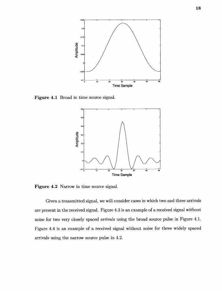
4.1 Broad in time source signal 18
4.2 Narrow in time source signal 18
4.3 Signal consisting of two arrivals closely spaced without noise for the broadtransmitted signal 19
4.4 Signal consisting of three arrivals widely spaced without noise for thenarrow transmitted signal 19
4.5 Signal obtained at the receiver for three arrivals with noise variance 0.01 20
4.6 Signal obtained at the receiver for three arrivals with noise variance 0.05 21
4.7 Signal obtained at the receiver for three arrivals with noise variance 0.1 . 21
4.8 Mean L i errors for delays only with noise variance 0.01 28
4.9 Mean L i errors for delays only with noise variance 0.05 29
4.10 Mean L i errors for delays only with noise variance 0.1 29
4.11 Samples obtained by EM for amplitude of the first arrival 44
4.12 Samples obtained by EM for amplitude of the second arrival 44
4.13 Distributions obtained by Gibbs sampling 49
5.1 Source signal 52
5.2 Signal obtained at the receiver for three arrivals widely spaced with noisevariance 0.01 53
5.3 Signal obtained at the receiver for three arrivals widely spaced with noisevariance 0.05 53
5.4 Signal obtained at the receiver for three arrivals widely spaced with noisevariance 0.1 54
5.5 Distributions for the variance obtained from 10 runs of the Gibbs samplingalgorithm for the wide arrival signal. The true variance is 0.01 . . . . 54
xii
LIST OF FIGURES(Continued)
Figure Page
5.6 Distributions for the variance obtained from 10 runs of the Gibbs samplingalgorithm for the wide arrival signal. The true variance is 0.05 . . . . 55
5.7 Distributions for the variance obtained from 10 runs of the Gibbs samplingalgorithm for the wide arrival signal. The true variance is 0.1 55
5.8 Distributions for the variance obtained from 10 runs of the Gibbs samplingalgorithm for the close arrival signal. The true variance is 0.01 . . . . 56
5.9 Distributions for the variance obtained from 10 runs of the Gibbs samplingalgorithm for the close arrival signal. The true variance is 0.05 . . . . 57
5.10 Distributions for the variance obtained from 10 runs of the Gibbs samplingalgorithm for the close arrival signal. The true variance is 0.1 57
5.11 Time delay and amplitude distributions obtained by Gibbs sampling withtrue variance 58
5.12 Time delay and amplitude distributions obtained by Gibbs sampling withwrong variance of 0.1 (true variance is 0.05) 58
6.1 Source signal 60
6.2 Distributions obtained by Gibbs sampling assuming two arrivals for thewide arrival signal with variance 0.01 61
6.3 Distributions obtained by Gibbs sampling assuming three arrivals arepresent for the wide arrival signal with variance 0.01 61
6.4 Distributions obtained by Gibbs sampling assuming four arrivals for thewide arrival signal with variance 0.01 61
6.5 Distributions obtained by Gibbs sampling assuming two arrivals for thewide arrival signal with variance 0.05 62
6.6 Distributions obtained by Gibbs sampling assuming three arrivals arepresent for the wide arrival signal with variance 0.05 63
6.7 Distributions obtained by Gibbs sampling assuming four arrivals for thewide arrival signal with variance 0.05 63
6.8 Distributions obtained by Gibbs sampling assuming two arrivals for thewide arrival signal with variance 0.1 64
6.9 Distributions obtained by Gibbs sampling assuming three arrivals arepresent for the wide arrival signal with variance 0.1 64
LIST OF FIGURES(Continued)
Figure Page
6.10 Distributions obtained by Gibbs sampling assuming four arrivals for thewide arrival signal with variance 0.1 65
6.11 Mean probability for the given number of arrivals 68
7.1 Samples for the time delay for the first arrival at each iteration 70
7.2 Samples for the time delay for the second arrival at each iteration . . 71
7.3 Samples for the time delay for the third arrival at each iteration 71
7.4 Samples for the amplitude for the first arrival at each iteration 72
7.5 Samples for the amplitude for the second arrival at each iteration . . 72
7.6 Samples for the amplitude for the third arrival at each iteration 73
7.7 Samples obtained by Gibbs sampling for the time delay for first arrival 76
7.8 Samples obtained by Gibbs sampling for the amplitude for the first arrivalat each iteration. The correct amplitude is 100 77
7.9 Samples obtained by Gibbs sampling for the amplitude for the secondarrival at each iteration. The correct amplitude is -80 78
7.10 Samples obtained by Gibbs sampling for the amplitude for the first arrivalat each iteration. The correct amplitude is 100 78
7.11 Samples obtained by Gibbs sampling for the amplitude for the secondarrival at each iteration. The correct amplitude is -80 79
7.12 Samples obtained by Gibbs sampling for the amplitude of the first arrivalvs. iteration. The correct amplitude is 100 79
7.13 Samples obtained by Gibbs sampling for the amplitude of the secondarrival vs. iteration. The correct amplitude is -80. 80
8.1 Real data from the Haro Straight experiment 82
8.2 Transmitted signal for real data from the Haro Straight experiment . . 83
8.3 Probability the signal in Figure 8.1 contains a given number of arrivals . 85
8.4 Samples for the first time delay from three runs of the Gibbs sampler . . 86
8.5 Samples for the variance from three different runs of the Gibbs sampler . 87
xiv
CHAPTER 1
INTRODUCTION
1.1 Motivation
In the last few decades, there has been explosive growth in the development of
numerical models used as tools in research involving underwater acoustics. One
particular area of interest in underwater acoustics is the propagation of sound in
a shallow ocean environment. The reason, in part, for such interest is the way
submarines are constructed today. First, some submarines, such as those which
transport navy seals, are much smaller than they were years ago. Their compact
size now allows the submarines to maneuver into more shallow water. Second, the
submarines are designed to be much quieter than they were in the past. This makes
them more difficult to detect. The harder these sounds are to detect, the easier it
is for these vessels to approach land, and hence, travel into shallow water. These
sounds, if detected, can be linked to a sound propagation model for the estimation of
source location.
Difficulties arise when one attempts to predict propagation of sound in a shallow
water ocean environment. The difficulty stems from the fact that a signal travelling in
shallow water will interact multiple times with both the ocean's surface and bottom.
In addition to knowing the source location and receiver location, as well as the
properties of the water, such as sound speed and depth of the water column, we also
need information about the parameters associated with the ocean bottom. We need
to identify the layers of the ocean bottom that the transmitted signal has interacted
with and how this interaction affects the received signal. Then, for each layer in the
bottom, we need to know the sound speed, density, attenuation and thickness of the
sediment. Thus, there has been strong motivation for the development of fast and
1
2
accurate inversion models for the concurrent estimation of location and environmental
parameters. In [1, 2, 3, 4, 5] it was shown that linking arrival times and amplitudes
of received time series to acoustic models, we can extract valuable information on
the environment and the location of the sound emitting source. However, accurate
identification of arrival times and amplitudes is not always simple. This identification
is the focus of this work.
1.2 Environment
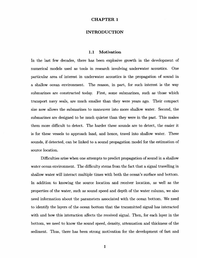
We are interested in modelling sound phenomena generated by a source and received
by a hydrophone in a range-independent shallow water ocean environment. In shallow
water, signals transmitted from an acoustic source usually arrive at the receiver
through multi-path propagation. Figure 1.1 shows three typical paths the rays will
take in travelling from the source to the receiver; there is a ray that goes directly
from the source to the receiver, a ray that is reflected off the ocean surface, and a ray
that is reflected off the ocean bottom before they reach the receiver.
Figure 1.1 Typical ray paths.
Thus the received signal in a shallow water environment, as well as in many
other problems in signal processing, can be modelled as a superposition of a finite
number of signals embedded in noise. These signals consist of delayed and attenuated
replicas of the transmitted signal due to various interactions with the boundaries. The
3
received signal can be generally written as:
r(n) = E as(n — ni) w(n).
M is the number of arrivals, ail and ni are the amplitude and time delay of the ith
arrival, and w(n) is additive noise.
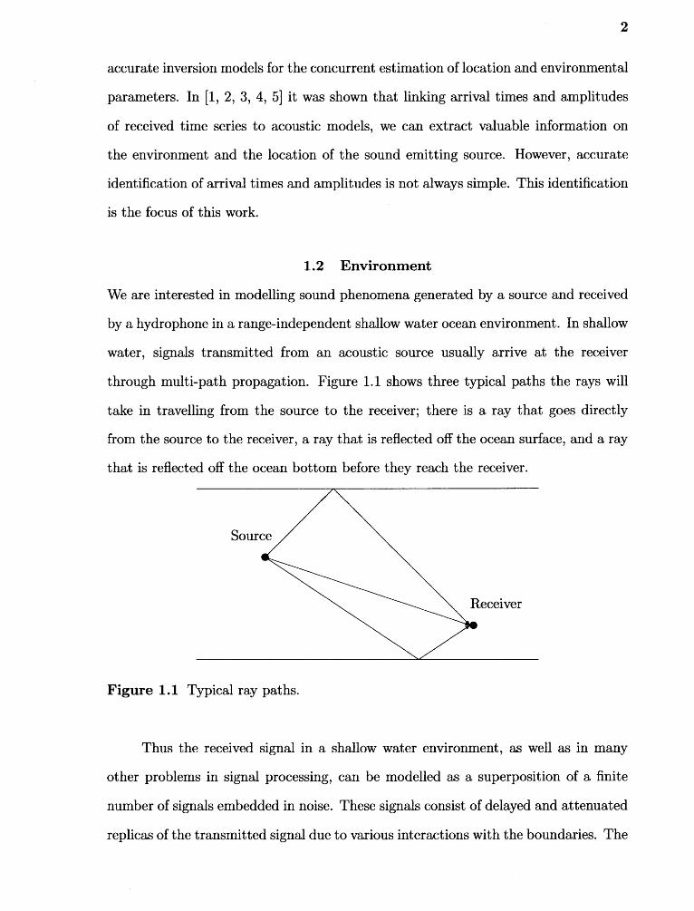
Figure 1.2 captures some of the features associated with arrivals corresponding
to distinct paths. This figure, however, is an over-simplification of an actual signal
obtained at a receiver because it does not include noise and it reflects the case of
undistorted high frequency signals.
0.05
0.04
0.03
0.020.05
E
- 0.05
- 0.02
- 0.03
- 0.04
-0.055.28
i i i i i i i i
5.3 5.32 5.34 5.36 5.38 5.4 5.42 5.44 5.46
5.48Time Delay
Figure 1.2 Signal obtained at the receiver.
The "spikes" in Figure 1.2 are the arrivals that we want to identify. Each arrival
has a time delay, due to the varying arrival times of the multi-paths, and amplitude
associated with it. The distinct arrivals correspond to rays which have travelled
along different paths from the source to the receiver. The first arrival is typically the
ray which travelled directly from the source to the receiver. The second arrival has
often gone through one surface reflection before reaching the receiver. The surface
reflected path is recognized by the change in polarity. The third arrival is the first
4
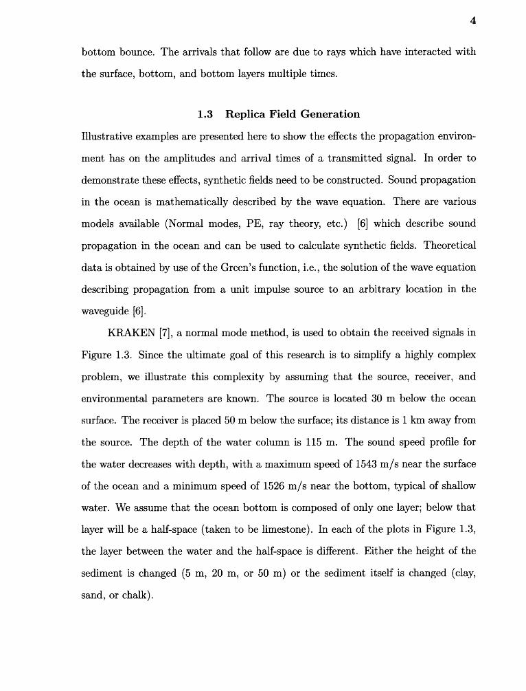
bottom bounce. The arrivals that follow are due to rays which have interacted with
the surface, bottom, and bottom layers multiple times.
1.3 Replica Field Generation
Illustrative examples are presented here to show the effects the propagation environ-
ment has on the amplitudes and arrival times of a transmitted signal. In order to
demonstrate these effects, synthetic fields need to be constructed. Sound propagation
in the ocean is mathematically described by the wave equation. There are various
models available (Normal modes, PE, ray theory, etc.) [6] which describe sound
propagation in the ocean and can be used to calculate synthetic fields. Theoretical
data is obtained by use of the Green's function, i.e., the solution of the wave equation
describing propagation from a unit impulse source to an arbitrary location in the
waveguide [6].
KRAKEN [7], a normal mode method, is used to obtain the received signals in
Figure 1.3. Since the ultimate goal of this research is to simplify a highly complex
problem, we illustrate this complexity by assuming that the source, receiver, and
environmental parameters are known. The source is located 30 m below the ocean
surface. The receiver is placed 50 m below the surface; its distance is 1 km away from
the source. The depth of the water column is 115 m. The sound speed profile for
the water decreases with depth, with a maximum speed of 1543 m/s near the surface
of the ocean and a minimum speed of 1526 m/s near the bottom, typical of shallow
water. We assume that the ocean bottom is composed of only one layer; below that
layer will be a half-space (taken to be limestone). In each of the plots in Figure 1.3,
the layer between the water and the half-space is different. Either the height of the
sediment is changed (5 m, 20 m, or 50 m) or the sediment itself is changed (clay,
sand, or chalk).
5
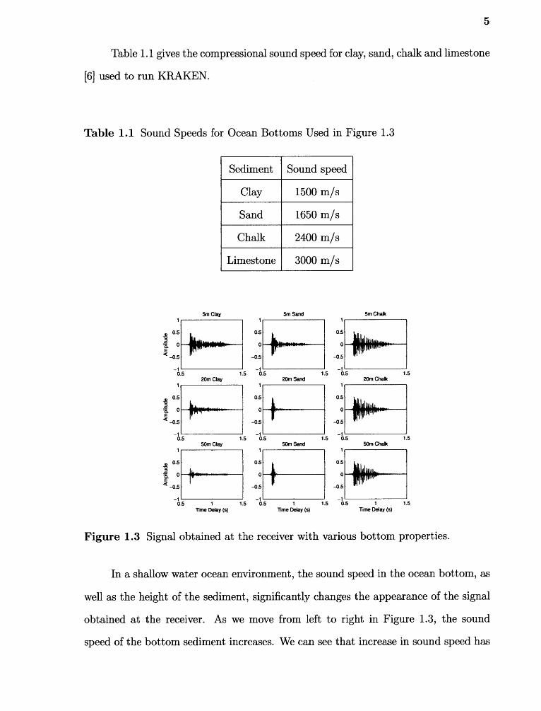
Table 1.1 gives the compressional sound speed for clay, sand, chalk and limestone
[6] used to run KRAKEN.
Table 1.1 Sound Speeds for Ocean Bottoms Used in Figure 1.3
Sediment Sound speed
Clay 1500 m/s
Sand 1650 m/s
Chalk 2400 m/s
Limestone 3000 m/s
0.5
0
- 0.5
-105
5m Clay 5m Sand 5m Chalk
0.5
- 0.5
-1 15 05 15
--111114000•••••.----
20m Clay1
20m Sand 20m Chalk
a 0.5 0.5 0.5
Tx 0 0
a _0.5 -0.5 -0.5
-1 -1 -1 05
15 05
15
0.5 1 550m Clay 50m Sand
50m Chalk
1
a 0.5-0= 0
a -0.5
-105
0.5
0
- OS
-11 15 05
Time Delay (s)
-1 1 15
05 1 15Time Delay (s) Time Delay (s)
0.5
0
- 0.5
Figure 1.3 Signal obtained at the receiver with various bottom properties.
In a shallow water ocean environment, the sound speed in the ocean bottom, as
well as the height of the sediment, significantly changes the appearance of the signal
obtained at the receiver. As we move from left to right in Figure 1.3, the sound
speed of the bottom sediment increases. We can see that increase in sound speed has
6
affected the amplitude of the signal, particularly at later times. As we move from
top to bottom in Figure 1.3, the height of the bottom layer is increased while the
sediment remains unchanged. Once again, we can see that a change in the height
of the sediment has an impact on the signal. We have acquired simulated data for
several test ocean bottom (basalt, limestone, chalk, moraine, gravel, sand, silt and
clay for example) and various sediment heights. Studying the received signals, it is
evident that the appearance of the signal is a direct consequence of the environment
the signal propagated through.
A typical approach for extracting information from received acoustic fields is
to use an inverse method which is generally cast as an optimization problem. In
this framework, we will concentrate on the appearance of the received signal. The
features associated with the signal we are interested in are the time delays and
amplitudes of each arrival as well as the Signal to Noise Ratio (SNR). (Time delay
and amplitude estimation is important in applications where a transmitted signal
arrives at a receiving sensor through different propagation paths.) These features
will form a basis for future estimation, reducing the computational time needed for
the implementation of full-field inverse method. As shown in Figure 1.3, the various
bottom sediments affect the amplitudes and the changes in sediment thickness affect
the time delays. Therefore, the focus of this work is to develop an efficient method
to easily recover these amplitudes and time delays, since they can provide significant
information on the propagation environment and geometry.
This dissertation is structured as follows: In Chapter 2 a brief overview of
methods typically applied to the problem at hand is provided. The Gibbs sampling
algorithm is derived and results for amplitude and time delay estimation are presented
and compared to other methods in Chapters 3 and 4. Noise is added in the estimation
process in Chapter 5 and results are presented. In Chapter 6 the number of arrivals
in the received signal is treated as an unknown. Chapter 7 deals with the issue of
7
convergence of the Gibbs sampling process. The number of arrivals, time delays,
amplitudes, and noise level are estimated for the real data from the Haro Straight
experiment in Chapter 8. Conclusions are given in Chapter 9.
CHAPTER 2
APPROACHES TO PARAMETER ESTIMATION PROBLEMS
Matched field processing (MFP) has been a popular approach for source localization
and parameter estimation in the ocean [8, 9]. MFP is a full-field matching approach.
It requires the replica field, which corresponds to theoretical array data, to be construc-
ted for each test ocean environment. Maximization of similarity between the replicas,
derived from the wave equation, and the data, measured at an array of sensors, is
then employed using correlation techniques to determine parameter estimates. This
process can become extremely computationally intensive due to the large number
of parameters involved. For example, one may only be interested in locating the
source, yet many other parameters associated with the environment such as sound
speed profile, water depth, bottom properties, etc. need to be taken into account.
Therefore, several approaches for reducing the computational requirements of MFP
have been proposed [10, 11, 12, 5].
An alternative approach to MFP is to perform the estimation in two steps. The
first step in the process is to obtain estimates for the parameters associated with
the received signal, for example, the amplitudes and time delays, noise variance, the
number of arrivals, etc. These estimates can then be used to quickly find estimates for
the parameters associated with the problem of interest, such as source and receiver
location, sound speed profile, bottom properties, etc. This work will focus on the
first step; we will concentrate only on select features of the synthetic field, extending
work presented in [12, 13, 14, 5, 15].
Previous work has been done on amplitude and arrival time estimation. Analyti-
cal Estimation [16J], Matched Filter (MF) [16, 171], Expectation Maximization (EM)
[12, 18], and Simulated Annealing (SA) algorithms [13] have been implemented to
8
9
identify these features. In this work, we develop a Gibbs sampling approach for
amplitude and arrival time estimation. We will compare our results using Gibbs
sampling to those obtained using the analytical estimation method, MF, EM, and
SA. Therefore, for the sake of completeness, we will provide a brief outline of the
major components involved in analytical estimation [16], MF [16, 17], EM [12], and
SA [10, 11, 13, 19].
In this paper, the method referred to as the analytical method is a maximum-
likelihood procedure for estimating the amplitudes and arrival times of individual
pulses in the multi-path signal [16]. Estimates of the N sets of amplitude and arrival
times can be obtained by formulating a 2N parameter estimation problem. First, the
maximum-likelihood estimates of arrival times for N pulses are obtained by finding
the maximum over ni of 13TA(I where (I) is the vector of matched filter outputs for
a particular set of arrival times n i and A is the cross-correlation matrix for the N
signals with delays n i , n2, ..., no. In general, there is no simple technique for finding
this maximum. The only recourse is to calculate (13 TA(I over a N-dimensional volume
in time space. The resulting set of arrival time estimates is then used in A = A -i (I)
to obtain the amplitude estimates. The computational demands required by this
estimation method quickly becomes overwhelming when the signal at hand has four
arrivals or more.
A Matched Filter (MF) can be used to recover the amplitudes and time delays of
a received signal. MF is favorable due to the ease in which it is implemented, simply
correlating each arrival in the received signal with the transmitted waveform [16, 17].
The time at which the filter output peaks gives the arrival time and the height of
the peak gives the amplitude. Difficulty will arise with the MF technique when the
arrival times of the received signal are close. Resolving individual waveforms in the
case of overlapping arrivals using MF could be erroneous [2, 13]. However, it can be
shown that, if the arrivals are separated in time by more than the duration of the
10
signal autocorrelation function, MF is equivalent to maximum likelihood estimation
(MLE) [16].
The EM algorithm is an iterative technique for solving MLE problems [11, 10].
The algorithm starts with an initial guess. EM is a two step process involving the
log-likelihood of the observed data. The first step is to compute the conditional
expected value of the unknown parameters given a signal. The second step in the
EM algorithm is to maximize the expected value found in the first step over all the
unknown parameters. EM is fast and works well with the proper initial conditions.
However, its performance is highly dependent on the initial conditions; the method
is quick to converge to a local maximum. As in all "hill climbing" techniques there
is no guarantee of convergence to a global maximum. Therefore, a "randomized hill
climbing" technique, referred to as SA, is more promising from this aspect, although
for this scheme global convergence in practice is not guaranteed [12, 11, 11] either.
SA is a Monte Carlo optimization approach [13]; it arose from the technique used
to slowly cool liquid metal to a crystal of minimum energy. Each parameter is given
an initial value. This initial value is perturbed through an addition of a random
component. The algorithm begins at a "high" temperature T. This temperature,
when high, increases the probability that we will accept the new values for the
parameters regardless of whether they are good or not. As the temperature decreases,
so does the probability of accepting a "bad" value. Starting at a "high" temperature
allows the algorithm to jump out of local minima. The core of SA is choosing the
appropriate cost function, annealing schedule, and suitable parameter perturbations.
The cost function is the quantity we wish to minimize (like the energy of the crystal).
The annealing schedule determines how T will be decreased. Choosing the appropriate
cost function and a good cooling schedule is critical to the success of an SA algorithm.
In this work, we present a novel method for estimation of time delays, amplitudes,
and number of multi-paths, as well as noise variance with a maximum a posteriori
11
estimation approach. Maximum a posteriori estimation is optimal if the appropriate
statistical models are selected for the received data. We propose a method of maximum
a posteriori estimation in which optimization is performed using Gibbs sampling
[24, 25, 26, 27, 28].
CHAPTER 3
GIBBS SAMPLING FOR PARAMETER ESTIMATION
To efficiently estimate the arrival times and amplitudes of a multi-path signal, we
propose a scheme that maximizes the posterior probability density function of those
unknowns. Noise variance and number of arrivals of arrivals are presently considered
as known parameters; this assumption will be removed in future chapters. To obtain
the posterior distribution of the arrival times and amplitudes, a standard Bayesian
approach is followed. That is, given received data, r, and a set of unknown parameters,
a, the joint probability distribution, p(r, a), is
p(r, a) = p(rla)p(a) = p(alr)p(r), (3.1)
and the a posteriori probability of a is given by:
p(alr) = p(rla)p(a) p(r) •
(3.2)
Selecting the values of a that maximize p(air) is known as maximum a posteriori
(MAP) estimation [29, 16]. Since p(r) is independent of the parameter a, maximizing
the a posteriori density is equivalent to maximizing the product p(ria)p(a) [19]. The
method is very powerful. The results, however, are dependent on the accuracy of the
statistical model p(ra) and the nature of prior beliefs encapsulated in p(a).
In [19] it is shown that if the prior distribution of a is broad and void of peaks,
there is a lack of any real knowledge on parameter a, except potentially for the limits
on the range of a. In this event, maximizing p(alr) is equivalent to maximizing
p(r la), which is known as maximum-likelihood estimation. As shown in [16], this is
the optimal approach to estimating time delays between distinct signals and their
corresponding amplitudes in a white Gaussian noise environment (a simple matched
12
13
filter is not optimal for overlapping arrivals). This maximization given observed data
leads to an analytical expression for the amplitudes, whereas time delays can be
obtained by identifying where the maximum of an M dimensional function occurs,
where M is the known number of paths [16]. When M is large, time delay estimation
becomes a computationally cumbersome task.
To alleviate some of the computational demands, we will use a Gibbs sampling
technique to efficiently estimate the posterior distribution of all unknown parameters
[14, 15]. The Gibbs sampler is a Monte Carlo Markov Chain approach for the
calculation of a numerical estimate of posterior probability distributions. In [26,
17, 15, 18] it is shown that the posterior distribution to be estimated is uniquely
determined through the conditional distributions of individual parameters.
3.1 Derivation of the Gibbs Sampler
In order to implement the Gibbs sampler for the purpose of estimating the unknown
parameters in our problem, the conditional distributions of time delays and amplitudes
need to be obtained. Equation 1.1 is used as a model for the received signal, where
w(n) is white Gaussian noise with zero mean and noise variance o -2 .
In our case, the amplitudes are real numbers and the sign indicates their polarity.
Since this is the only prior information available on the amplitudes, uniform, non-
informative prior distributions for these parameters are assumed. That is,
p(ai) = 1, —co < a i < d-oo, i = 1, ..., M. (3.3)
For the time delays, we will assume uniform priors for arrival times that vary between
1 and A, i.e.,
1p(ai ) =
' 1 < ni < A' i — 1 M •
(3.4)
14
The joint posterior probability distribution function of all unknown parameters
ailand ni, i = 1, ...,Mgiven observed data r(n) can be written as follows [30, 31, 31]:
p(ni, ..., Om , al, ...,am lr(n)) =
1 1 1 N M
K N" (1117)
ouoexp( 1o-2
E (r(A) — E ais(n — n2 )) 2 ), (3.5)
where 1/K is the N-dimensional joint probability density function of r(A), n =
1, ..., N, which is a constant. Equation 3.5 can be simplified by consolidating all
constants:
P(ni, ...,Om, al, ..., amlr(n)) =1
N MCeXP(
1 2E (r(n) — E as(n — n))2).
From this joint posterior probability distribution function, an expression for the
conditional distribution of a ilcan be obtained assuming allail, j= 1, ...,M, ji and
all Lk , k =1,...,M are known. From Equation 3.6, the marginal posterior distribution
for a ilcan be obtained:
1Dexp(— 1,72 (cti —
P(ailn17o
(E r(n)s(nn=i
...,Am, a l , ..., ai+i , ai+i , ..., am , r(n)) =M N
— n i) — E ail > s(n — n i)s(n— n3)))2), (3.7)i=i(joi) n=i
where D is the normalization constant of the distribution. The distribution of
Equation 3.7 can be identified to be Gaussian with mean
o M oE r(L)s(L— L ib )— E aj E s(n — Li )s(L — nj ) (3.8)n=i j=1(j0i) n=i
n=i i=i
(3.6)n=i i=i
and variance o-2 .
15
The conditional posterior distributions for time delays n n , i = 1, M are
obtained on a grid. Assuming ail, j = 1, M and Lk , k = M, k i are
known, the conditional distribution of n n is written:
p(nilni , ...,Lm, al , ..., am , r(n)) =
1Gexp( — (On) — E as(n — n))2)
a2 n=1 n=1(3.9)
where G is the normalization constant of the distribution.
3.2 Gibbs Sampling Implementation
Gibbs sampling is a Monte Carlo Markov Chain approach that can be used to
obtain estimates for the arrival times and amplitudes of the distinct arrivals. It
is a technique for generating random samples from a joint posterior distribution
indirectly by drawing samples from conditional distributions [14, 28]. The Gibbs
sampling Markovian updating scheme proceeds as follows.
Given a received signal with M distinct arrivals, the algorithm begins by assign-
ing initial values to the 1M unknown parameters (each arrival has a time delay and
an amplitude associated with it). The Gaussian distribution of Equation 3.7 is used
to generate a sample for a l , which is conditional on all 2M — 1 other parameters
involved in the estimation. Using this new value for a l , a sample is generated for a 2 .
The updating process continues until a sample is generated for all a il , i = 1, ..., M.
The conditional distribution, Equation 3.9, is then used to obtain samples for each
N. However, since the posterior distributions of the time delays are not analytically
tractable, the distribution in Equation 3.9 will be calculated on a grid. Once a sample
has been generated for all 2M parameters one iteration is complete and the process
is continued repeatedly until many samples have been drawn for all parameters.
Reference [16] shows that under mild conditions, after many iterations, the samples
generated can be regarded as simulated observations from the true joint distribution.
16
And so, Gibbs sampling is based only on elementary properties of Markov chains
and avoids difficult calculations, replacing them instead with a sequence of easier
calculations [28].
Investigations have shown that iterative sampling achieved through Gibbs sam-
plers is efficient, converging quickly for a wide range of problems. Advocacy of the
approach rests on its simplicity and universality but not on any claim that it is the
most efficient procedure for any given problem [27]. This work will show that, for
the purpose of estimating time delays and amplitudes, the algorithm is not only
accurate and efficient but is also more informative than other estimation methods. It
provides estimates of the posterior probability distribution functions in addition to
point estimates typically provided by other approaches.
CHAPTER 4
PERFORMANCE EVALUATION OF ESTIMATION APPROACHES
In this chapter the proposed Gibbs sampling algorithm is tested on synthetic data and
compared to the optimal analytical method [16], MF, EM, and SA. Numerous received
signals are numerically simulated. These five methods are then used to calculate
estimates for the time delays and amplitudes for each arrival. Error measures are then
calculated in order to compare the performance of each algorithm. Also presented
in this chapter is an example in which one run of the Gibbs sampler appears to
fail to locate all the arrivals present in the received signal when only looking at the
point estimates obtained. However, it is shown that the distribution of all samples
generated provides information on the missed arrival.
4.1 Signal Generation
Received signals are numerically generated for two source signals. The first source
sequence is the broad in time, truncated sinc pulse shown in Figure 4.1. The second
source used to generate replicas of transmitted signals is the more narrow sinc pulse
shown in Figure 4.2. Arranging these signals at different places in time with various
amplitudes creates signals similar to those generated when a pulse travels to a receiver
by way of many paths.
17
18
Figure 4.1 Broad in time source signal.
20 30 40 50
Time Sample
Figure 4.2 Narrow in time source signal.
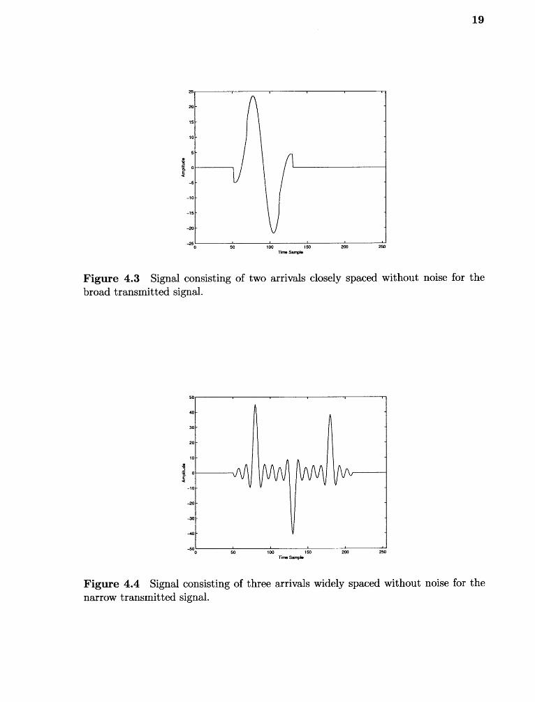
Given a transmitted signal, we will consider cases in which two and three arrivals
are present in the received signal. Figure 4.3 is an example of a received signal without
noise for two very closely spaced arrivals using the broad source pulse in Figure 4.1.
Figure 4.4 is an example of a received signal without noise for three widely spaced
arrivals using the narrow source pulse in 4.2.
50
30 -
20 -
10-
-10
-20
fa
50 100 150 200 250-50
0
15-
10
5
-10 -
-15 -
-20-
-250
50 100 150 200 250Time Sample
Figure 4.3 Signal consisting of two arrivals closely spaced without noise for thebroad transmitted signal.
Time Sample
19
=E
Figure 4.4 Signal consisting of three arrivals widely spaced without noise for thenarrow transmitted signal.
30 -
-5 0
50 500 550 200
1■
250
20
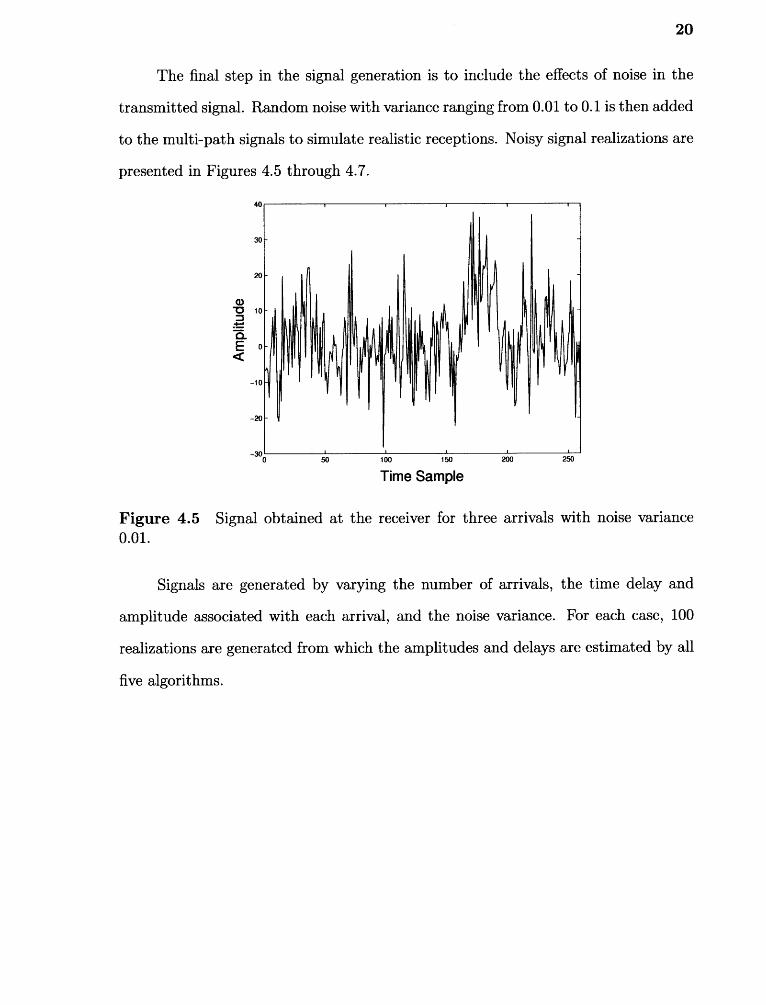
The final step in the signal generation is to include the effects of noise in the
transmitted signal. Random noise with variance ranging from 0.01 to 0.1 is then added
to the multi-path signals to simulate realistic receptions. Noisy signal realizations are
presented in Figures 4.5 through 4.7.
Time Sample
Figure 4.5 Signal obtained at the receiver for three arrivals with noise variance0.01.
Signals are generated by varying the number of arrivals, the time delay and
amplitude associated with each arrival, and the noise variance. For each case, 100
realizations are generated from which the amplitudes and delays are estimated by all
five algorithms.
500
21
a)V, P. .aE< ill
50 500 550
200
250
Time Sample
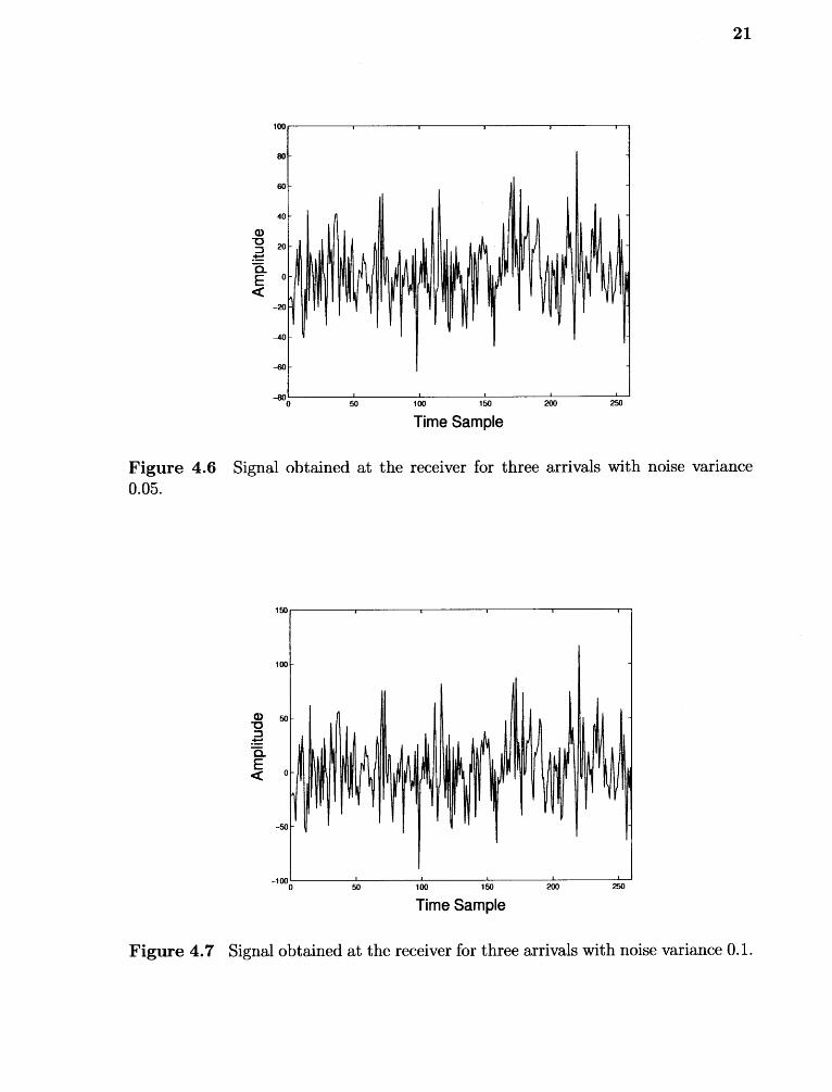
Figure 4.6 Signal obtained at the receiver for three arrivals with noise variance0.05.
50 500 550
200
250
Time Sample
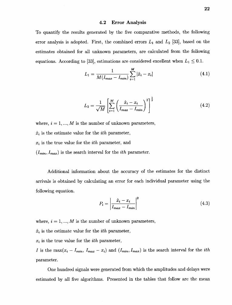
Figure 4.7 Signal obtained at the receiver for three arrivals with noise variance 0.1.
22
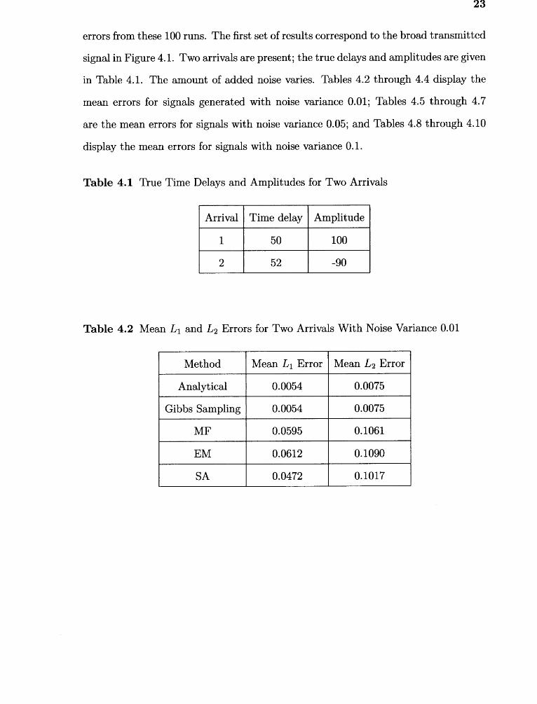
4.2 Error Analysis
To quantify the results generated by the five comparative methods, the following
error analysis is adopted. First, the combined errors L ib and L2 [33], based on the
estimates obtained for all unknown parameters, are calculated from the following
equations. According to [33], estimations are considered excellent when L ib < 0.1.
- mil= LibA ,A T
1V1 vintage 'min/ ti=i
1 M — Xi[L2 =
\FM— ti=i 'max
where, i = 1, M is the number of unknown parameters,
Xi is the estimate value for the ith parameter,
xi is the true value for the ith parameter, and
Image) is the search interval for the ith parameter.
Additional information about the accuracy of the estimates for the distinct
arrivals is obtained by calculating an error for each individual parameter using the
following equation.2
2
) 22
(4.1)
(4.2)
Pi =Image
(4.3)xi — xi
where, i = 1, M is the number of unknown parameters,
Xi is the estimate value for the ith parameter,
xi is the true value for the ith parameter,
I is the max(xi — min, Image — Xi) and (Imin , Image) is the search interval for the ith
parameter.
One hundred signals were generated from which the amplitudes and delays were
estimated by all five algorithms. Presented in the tables that follow are the mean
23
errors from these 100 runs. The first set of results correspond to the broad transmitted
signal in Figure 4.1. Two arrivals are present; the true delays and amplitudes are given
in Table 4.1. The amount of added noise varies. Tables 4.2 through 4.4 display the
mean errors for signals generated with noise variance 0.01; Tables 4.5 through 4.7
are the mean errors for signals with noise variance 0.05; and Tables 4.8 through 4.10
display the mean errors for signals with noise variance 0.1.
Table 4.1 True Time Delays and Amplitudes for Two Arrivals
Arrival Time delay Amplitude
1 50 100
2 52 -90
Table 4.2 Mean Li and L2 Errors for Two Arrivals With Noise Variance 0.01
Method Mean Lib Error Mean L2 Error
Analytical 0.0054 0.0075
Gibbs Sampling 0.0054 0.0075
MF 0.0595 0.1061
EM 0.0612 0.1090
SA 0.0472 0.1017
24
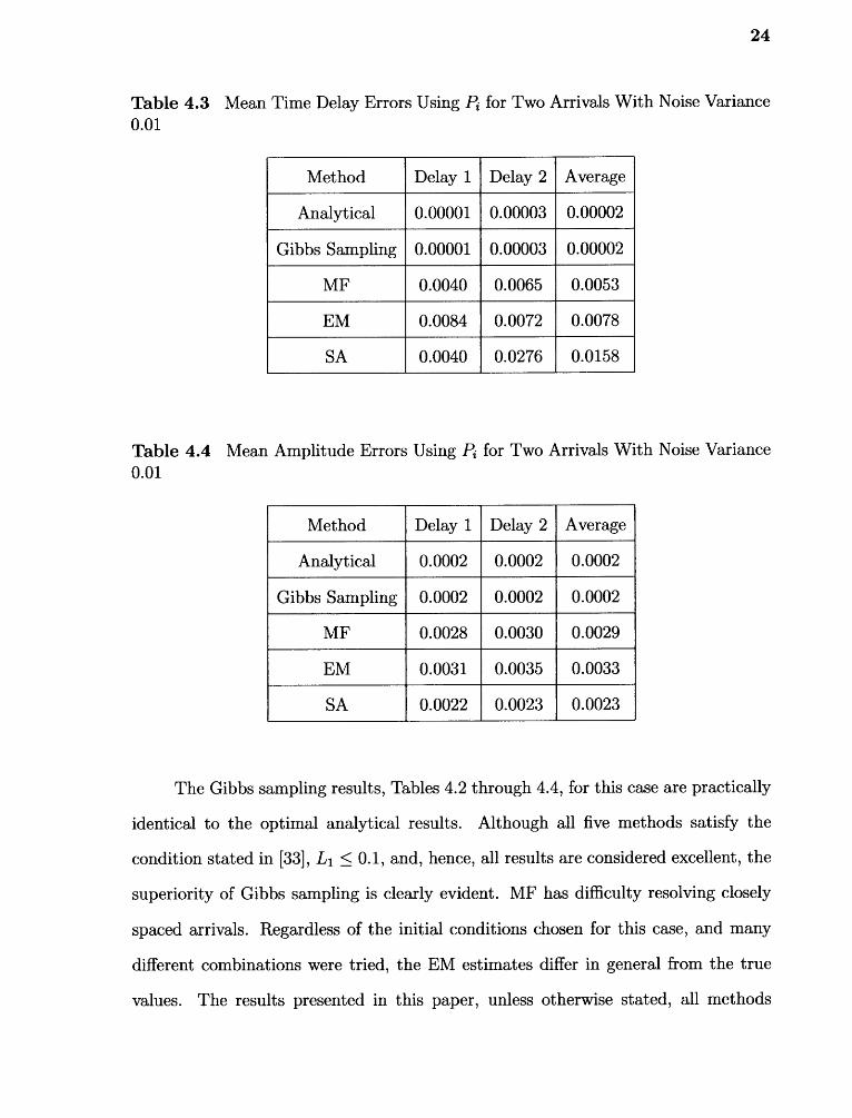
Table 4.3 Mean Time Delay Errors Using Pn for Two Arrivals With Noise Variance0.01
Method Delay 1 Delay 2 Average
Analytical 0.00001 0.00003 0.00002
Gibbs Sampling 0.00001 0.00003 0.00002
MF 0.0040 0.0065 0.0053
EM 0.0084 0.0072 0.0078
SA 0.0040 0.0276 0.0158
Table 4.4 Mean Amplitude Errors Using Pi for Two Arrivals With Noise Variance0.01
Method Delay 1 Delay 2 Average
Analytical 0.0002 0.0002 0.0002
Gibbs Sampling 0.0002 0.0002 0.0002
MF 0.0028 0.0030 0.0029
EM 0.0031 0.0035 0.0033
SA 0.0022 0.0023 0.0023
The Gibbs sampling results, Tables 4.2 through 4.4, for this case are practically
identical to the optimal analytical results. Although all five methods satisfy the
condition stated in [33], L i < 0.1, and, hence, all results are considered excellent, the
superiority of Gibbs sampling is clearly evident. MF has difficulty resolving closely
spaced arrivals. Regardless of the initial conditions chosen for this case, and many
different combinations were tried, the EM estimates differ in general from the true
values. The results presented in this paper, unless otherwise stated, all methods
25
requiring initial conditions, Gibbs sampling, EM, and SA, are started with the same
initial conditions for fair comparison. SA was generally unable to recover the second
arrival.
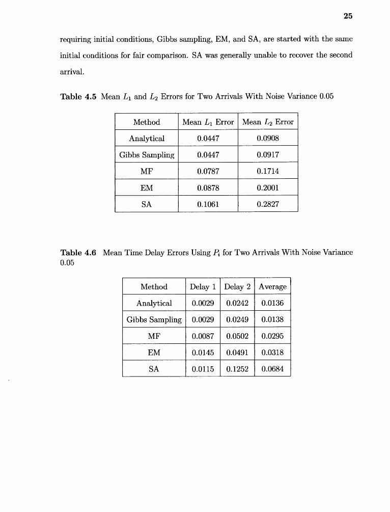
Table 4.5 Mean Lib and L2 Errors for Two Arrivals With Noise Variance 0.05
Method Mean L1 Error Mean L2 Error
Analytical 0.0447 0.0908
Gibbs Sampling 0.0447 0.0917
MF 0.0787 0.1714
EM 0.0878 0.2001
SA 0.1061 0.2827
Table 4.6 Mean Time Delay Errors Using Pn for Two Arrivals With Noise Variance0.05
Method Delay 1 Delay 2 Average
Analytical 0.0029 0.0242 0.0136
Gibbs Sampling 0.0029 0.0249 0.0138
MF 0.0087 0.0502 0.0295
EM 0.0145 0.0491 0.0318
SA 0.0115 0.1252 0.0684
26
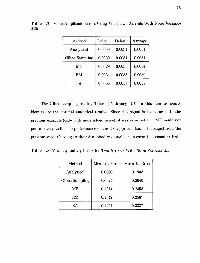
Table 4.7 Mean Amplitude Errors Using Pi for Two Arrivals With Noise Variance0.05
Method Delay 1 Delay 2 Average
Analytical 0.0030 0.0031 0.0031
Gibbs Sampling 0.0030 0.0031 0.0031
MF 0.0029 0.0038 0.0034
EM 0.0034 0.0038 0.0036
SA 0.0036 0.0037 0.0037
The Gibbs sampling results, Tables 4.5 through 4.7, for this case are nearly
identical to the optimal analytical results. Since this signal is the same as in the
previous example (only with more added noise), it was expected that MF would not
perform very well. The performance of the EM approach has not changed from the
previous case. Once again the SA method was unable to recover the second arrival.
Table 4.8 Mean Li and L2 Errors for Two Arrivals With Noise Variance 0.1
Method Mean L1 Error Mean L2 Error
Analytical 0.0880 0.1903
Gibbs Sampling 0.0925 0.2040
MF 0.1014 0.2358
EM 0.1042 0.2567
SA 0.1254 0.3337
27
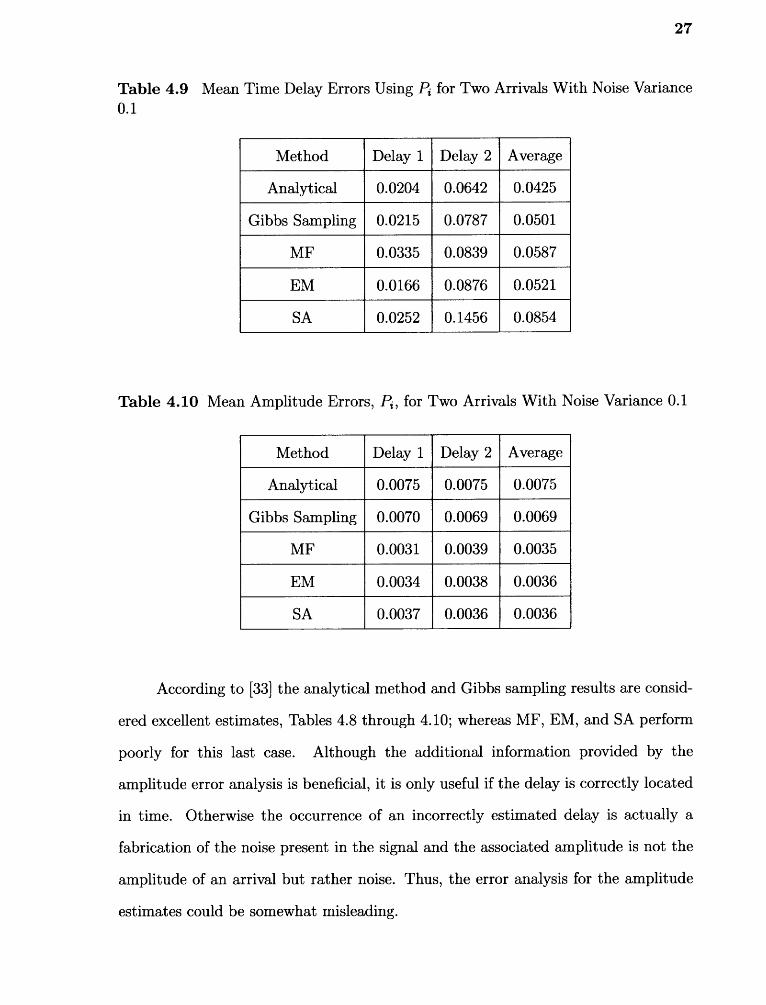
Table 4.9 Mean Time Delay Errors Using Pi for Two Arrivals With Noise Variance0.1
Method Delay 1 Delay 2 Average
Analytical 0.0204 0.0642 0.0425
Gibbs Sampling 0.0215 0.0787 0.0501
MF 0.0335 0.0839 0.0587
EM 0.0166 0.0876 0.0521
SA 0.0252 0.1456 0.0854
Table 4.10 Mean Amplitude Errors, Pi , for Two Arrivals With Noise Variance 0.1
Method Delay 1 Delay 2 Average
Analytical 0.0075 0.0075 0.0075
Gibbs Sampling 0.0070 0.0069 0.0069
MF 0.0031 0.0039 0.0035
EM 0.0034 0.0038 0.0036
SA 0.0037 0.0036 0.0036
According to [33] the analytical method and Gibbs sampling results are consid-
ered excellent estimates, Tables 4.8 through 4.10; whereas MF, EM, and SA perform
poorly for this last case. Although the additional information provided by the
amplitude error analysis is beneficial, it is only useful if the delay is correctly located
in time. Otherwise the occurrence of an incorrectly estimated delay is actually a
fabrication of the noise present in the signal and the associated amplitude is not the
amplitude of an arrival but rather noise. Thus, the error analysis for the amplitude
estimates could be somewhat misleading.
0 2 2015505
0.07
0.06
0.05
0.04
- Analytical- Gibbs sampling
MF- EM
SA
0.02
0.05
0
w0.03
28
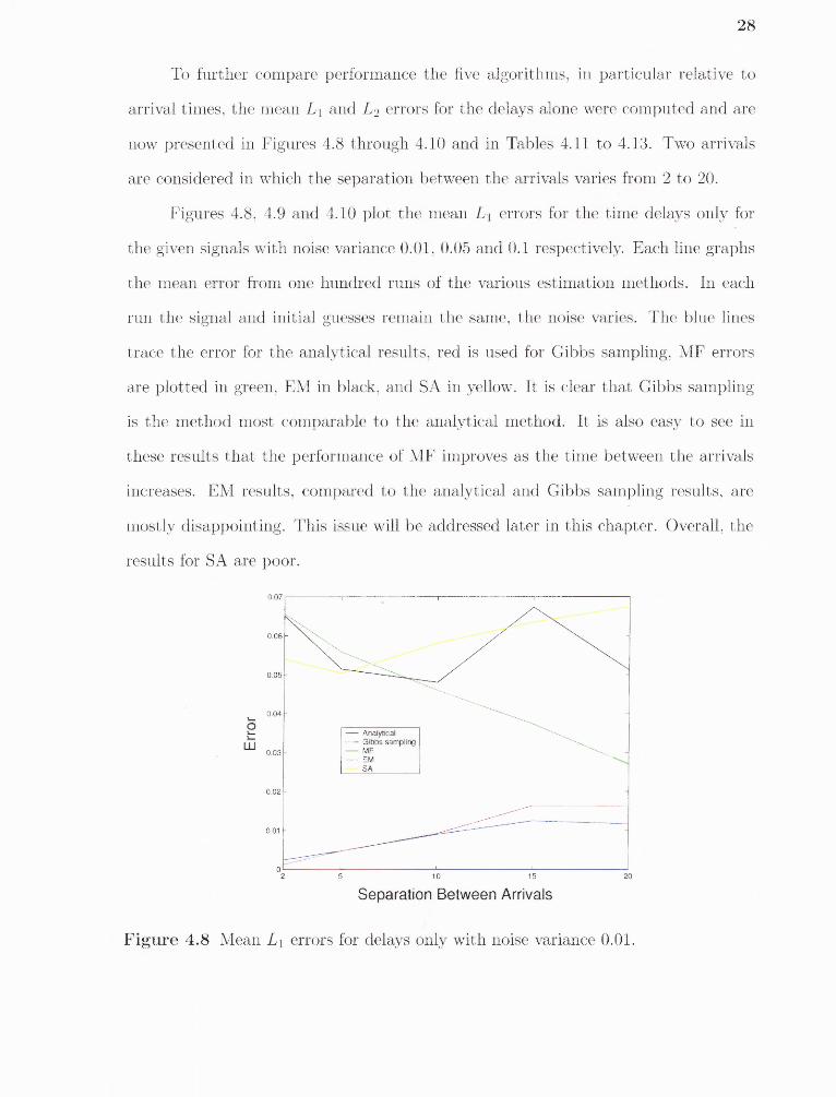
To further compare performance the five algorithms, in particular relative to
arrival times, the mean Li and L2 errors for the delays alone were computed and are
now presented in Figures 4.8 through 4.10 and in Tables 4.11 to 4.13. Two arrivals
are considered in which the separation between the arrivals varies from 2 to 20.
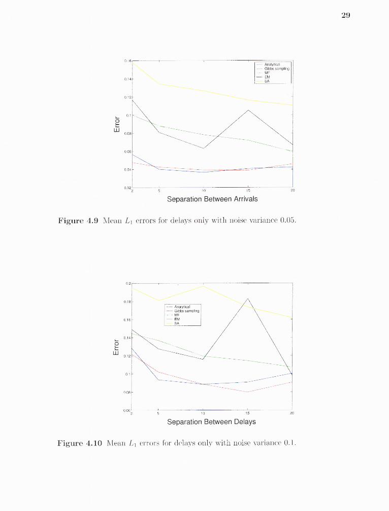
Figures 4.8, 4.9 and 4.10 plot the mean L1 errors for the time delays only for
the given signals with noise variance 0.01, 0.05 and 0.1 respectively. Each line graphs
the mean error from one hundred runs of the various estimation methods. In each
run the signal and initial guesses remain the same, the noise varies. The blue lines
trace the error for the analytical results, red is used for Gibbs sampling, MF errors
are plotted in green, EM in black, and SA in yellow. It is clear that Gibbs sampling
is the method most comparable to the analytical method. It is also easy to see in
these results that the performance of MF improves as the time between the arrivals
increases. EM results, compared to the analytical and Gibbs sampling results, are
mostly disappointing. This issue will be addressed later in this chapter. Overall, the
results for SA are poor.
Separation Between Arrivals
Figure 4.8 Mean Li errors for delays only with noise variance 0.01.
0.18- Analytical
Gibbs samplingMF
- EMSA
0.16
2w
0.14
0.12
0.5
0.08
5 10 1150.06
202
0.16
0.14
29
- Analytical- Gibbs sampling
MF- EM
SA
0.12
2w
0. 5
0.08
0.06
0.04
0.02 5
10
15
20
Separation Between Arrivals
Figure 4.9 Mean L 1 errors for delays only with noise variance 0.05.
Separation Between Delays
Figure 4.10 Mean L 1 errors for delays only with noise variance 0.1.
30
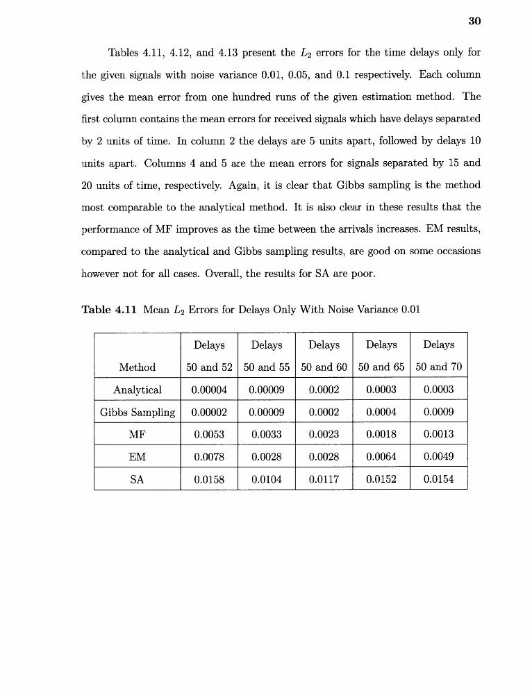
Tables 4.11, 4.12, and 4.13 present the L2 errors for the time delays only for
the given signals with noise variance 0.01, 0.05, and 0.1 respectively. Each column
gives the mean error from one hundred runs of the given estimation method. The
first column contains the mean errors for received signals which have delays separated
by 2 units of time. In column 2 the delays are 5 units apart, followed by delays 10
units apart. Columns 4 and 5 are the mean errors for signals separated by 15 and
10 units of time, respectively. Again, it is clear that Gibbs sampling is the method
most comparable to the analytical method. It is also clear in these results that the
performance of MF improves as the time between the arrivals increases. EM results,
compared to the analytical and Gibbs sampling results, are good on some occasions
however not for all cases. Overall, the results for SA are poor.
Table 4.11 Mean L2 Errors for Delays Only With Noise Variance 0.01
Method
Delays
50 and 52
Delays
50 and 55
Delays
50 and 60
Delays
50 and 65
Delays
50 and 70
Analytical 0.00004 0.00009 0.0002 0.0003 0.0003
Gibbs Sampling 0.00002 0.00009 0.0002 0.0004 0.0009
MF 0.0053 0.0033 0.0023 0.0018 0.0013
EM 0.0078 0.0028 0.0028 0.0064 0.0049
SA 0.0158 0.0104 0.0117 0.0152 0.0154
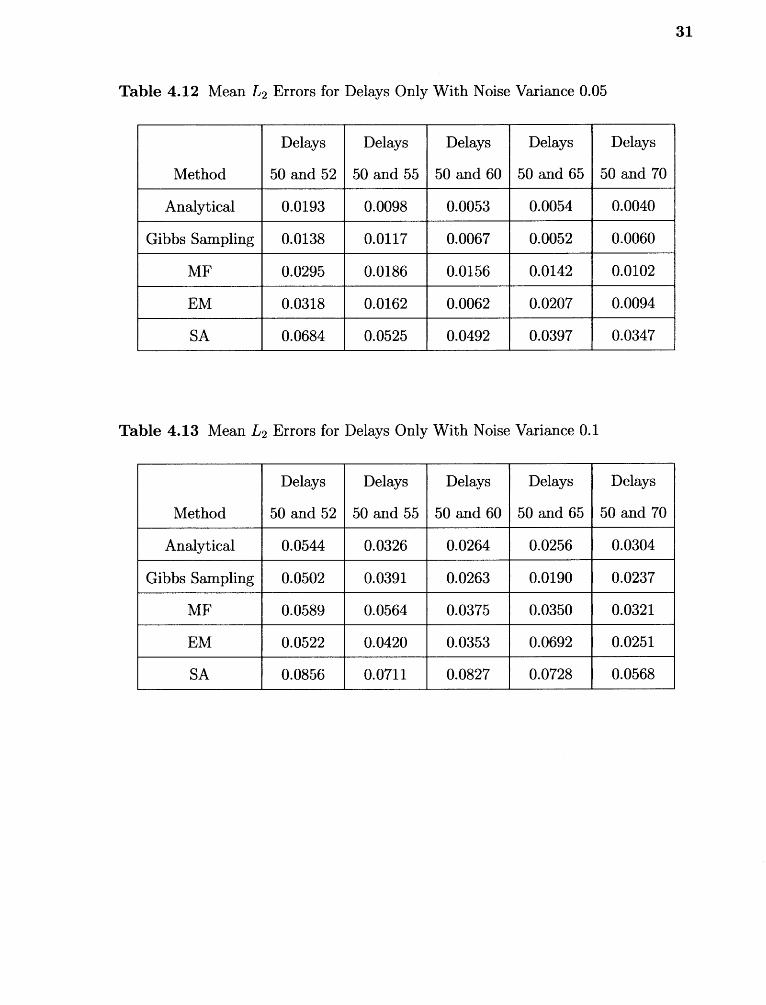
Table 4.12 Mean L2 Errors for Delays Only With Noise Variance 0.05
Method
Delays
50 and 52
Delays
50 and 55
Delays
50 and 60
Delays
50 and 65
Delays
50 and 70
Analytical 0.0193 0.0098 0.0053 0.0054 0.0040
Gibbs Sampling 0.0138 0.0117 0.0067 0.0052 0.0060
MF 0.0295 0.0186 0.0156 0.0142 0.0102
EM 0.0318 0.0162 0.0062 0.0207 0.0094
SA 0.0684 0.0525 0.0492 0.0397 0.0347
Table 4.13 Mean L2 Errors for Delays Only With Noise Variance 0.1
Method
Delays
50 and 52
Delays
50 and 55
Delays
50 and 60
Delays
50 and 65
Delays
50 and 70
Analytical 0.0544 0.0326 0.0264 0.0256 0.0304
Gibbs Sampling 0.0502 0.0391 0.0263 0.0190 0.0237
MF 0.0589 0.0564 0.0375 0.0350 0.0321
EM 0.0522 0.0420 0.0353 0.0692 0.0251
SA 0.0856 0.0711 0.0827 0.0728 0.0568
31
32
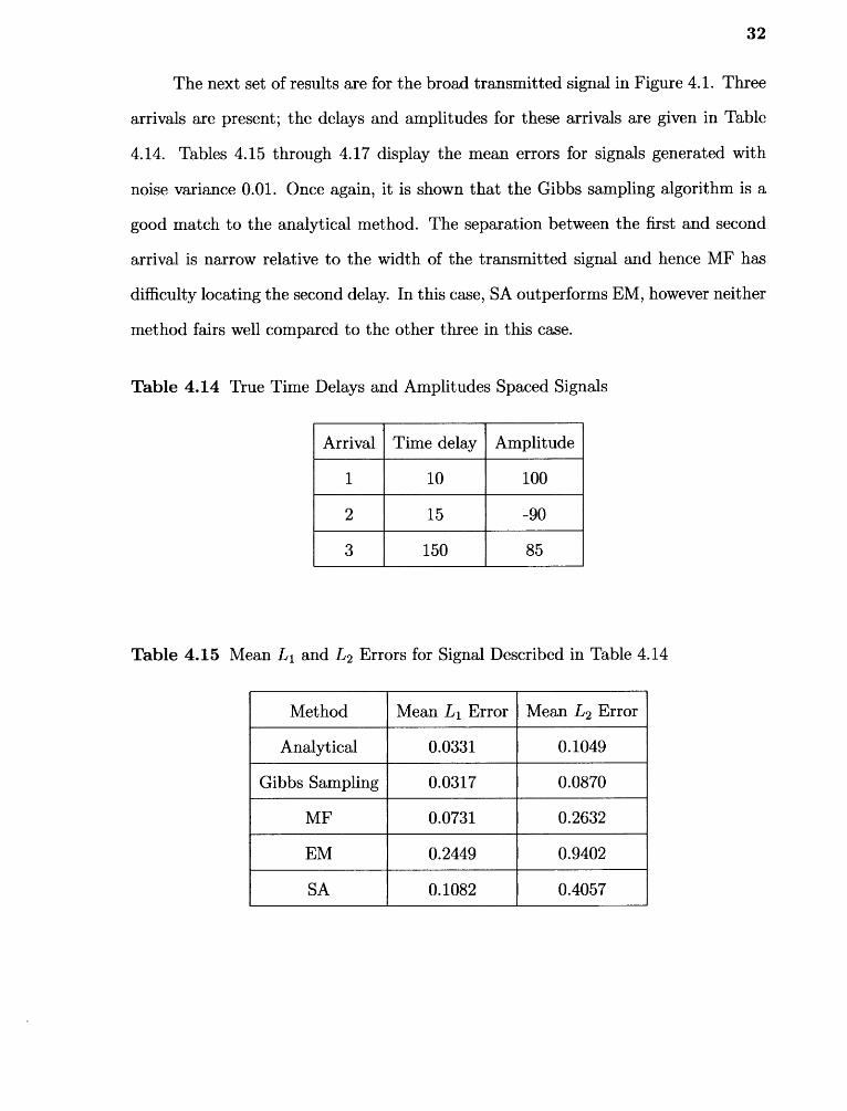
The next set of results are for the broad transmitted signal in Figure 4.1. Three
arrivals are present; the delays and amplitudes for these arrivals are given in Table
4.14. Tables 4.15 through 4.17 display the mean errors for signals generated with
noise variance 0.01. Once again, it is shown that the Gibbs sampling algorithm is a
good match to the analytical method. The separation between the first and second
arrival is narrow relative to the width of the transmitted signal and hence MF has
difficulty locating the second delay. In this case, SA outperforms EM, however neither
method fairs well compared to the other three in this case.
Table 4.14 True Time Delays and Amplitudes Spaced Signals
Arrival Time delay Amplitude
1 10 100
2 15 -90
3 150 85
Table 4.15 Mean Li and L2 Errors for Signal Described in Table 4.14
Method Mean Lib Error Mean L2 Error
Analytical 0.0331 0.1049
Gibbs Sampling 0.0317 0.0870
MF 0.0731 0.2632
EM 0.2449 0.9402
SA 0.1082 0.4057
33
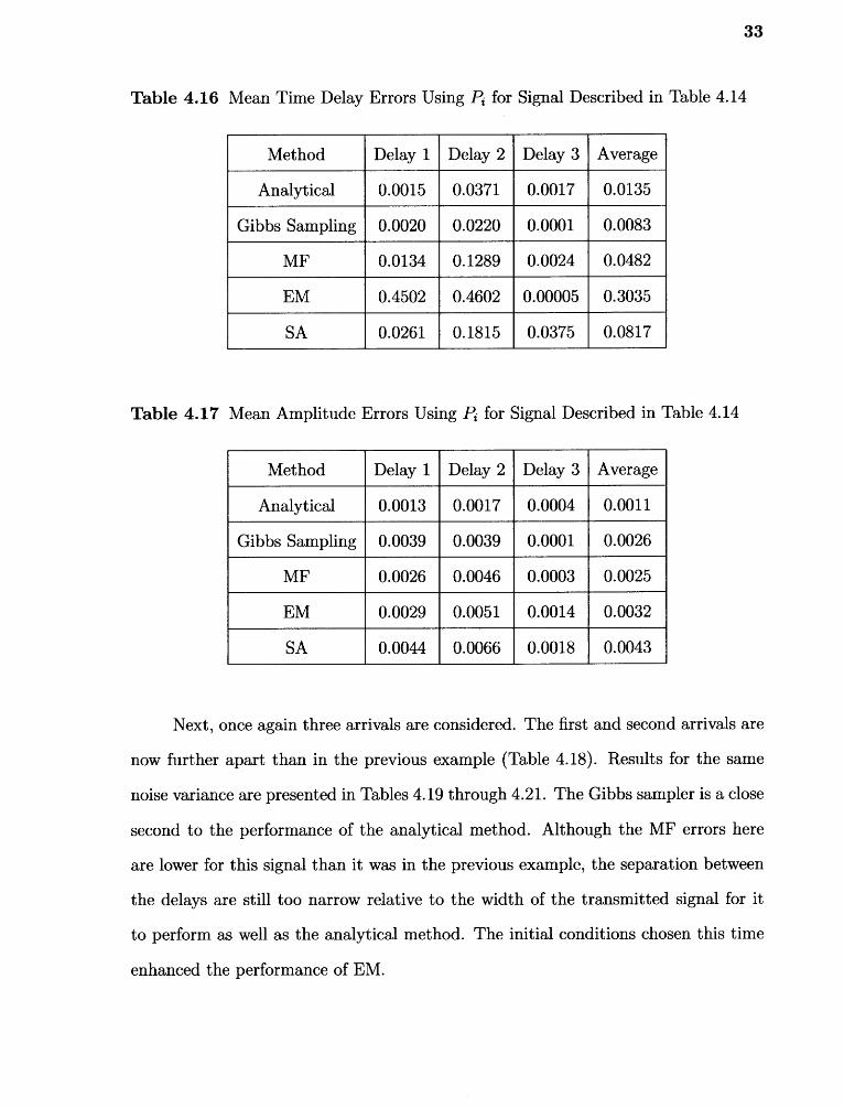
Table 4.16 Mean Time Delay Errors Using Pi for Signal Described in Table 4.14
Method Delay 1 Delay 2 Delay 3 Average
Analytical 0.0015 0.0371 0.0017 0.0135
Gibbs Sampling 0.0020 0.0220 0.0001 0.0083
MF 0.0134 0.1289 0.0024 0.0482
EM 0.4502 0.4602 0.00005 0.3035
SA 0.0261 0.1815 0.0375 0.0817
Table 4.17 Mean Amplitude Errors Using Pi for Signal Described in Table 4.14
Method Delay 1 Delay 2 Delay 3 Average
Analytical 0.0013 0.0017 0.0004 0.0011
Gibbs Sampling 0.0039 0.0039 0.0001 0.0026
MF 0.0026 0.0046 0.0003 0.0025
EM 0.0029 0.0051 0.0014 0.0032
SA 0.0044 0.0066 0.0018 0.0043
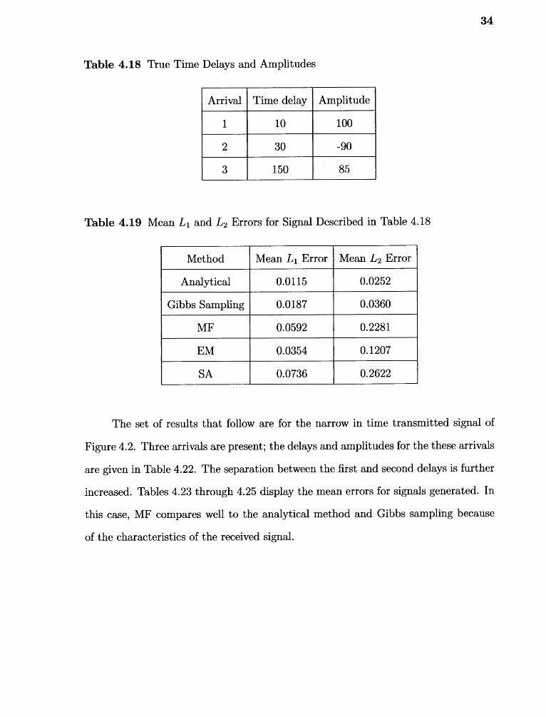
Next, once again three arrivals are considered. The first and second arrivals are
now further apart than in the previous example (Table 4.18). Results for the same
noise variance are presented in Tables 4.19 through 4.21. The Gibbs sampler is a close
second to the performance of the analytical method. Although the MF errors here
are lower for this signal than it was in the previous example, the separation between
the delays are still too narrow relative to the width of the transmitted signal for it
to perform as well as the analytical method. The initial conditions chosen this time
enhanced the performance of EM.
34
Table 4.18 True Time Delays and Amplitudes
Arrival Time delay Amplitude
1 10 100
2 30 -90
3 150 85
Table 4.19 Mean Lib and L2 Errors for Signal Described in Table 4.18
Method Mean Lib Error Mean L2 Error
Analytical 0.0115 0.0252
Gibbs Sampling 0.0187 0.0360
MF 0.0592 0.2281
EM 0.0354 0.1207
SA 0.0736 0.2622
The set of results that follow are for the narrow in time transmitted signal of
Figure 4.2. Three arrivals are present; the delays and amplitudes for the these arrivals
are given in Table 4.22. The separation between the first and second delays is further
increased. Tables 4.23 through 4.25 display the mean errors for signals generated. In
this case, MF compares well to the analytical method and Gibbs sampling because
of the characteristics of the received signal.
35
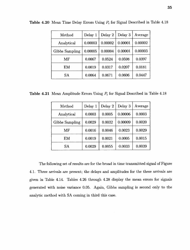
Table 4.20 Mean Time Delay Errors Using Pi for Signal Described in Table 4.18
Method Delay 1 Delay 2 Delay 3 Average
Analytical 0.00003 0.00002 0.00001 0.00002
Gibbs Sampling 0.00005 0.00004 0.00001 0.00003
MF 0.0067 0.0524 0.0598 0.0397
EM 0.0019 0.0317 0.0207 0.0181
SA 0.0064 0.0671 0.0606 0.0447
Table 4.21 Mean Amplitude Errors Using Pi for Signal Described in Table 4.18
Method Delay 1 Delay 2 Delay 3 Average
Analytical 0.0003 0.0005 0.00006 0.0003
Gibbs Sampling 0.0029 0.0032 0.00009 0.0020
MF 0.0016 0.0046 0.0023 0.0029
EM 0.0019 0.0021 0.0005 0.0015
SA 0.0029 0.0055 0.0033 0.0039
The following set of results are for the broad in time transmitted signal of Figure
4.1. Three arrivals are present; the delays and amplitudes for the these arrivals are
given in Table 4.14. Tables 4.26 through 4.28 display the mean errors for signals
generated with noise variance 0.05. Again, Gibbs sampling is second only to the
analytic method with SA coming in third this case.
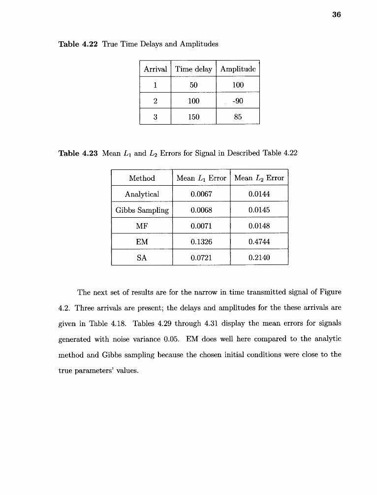
36
Table 4.22 True Time Delays and Amplitudes
Arrival Time delay Amplitude
1 50 100
2 100 -90
3 150 85
Table 4.23 Mean Lib and L2 Errors for Signal in Described Table 4.22
Method Mean Lib Error Mean L2 Error
Analytical 0.0067 0.0144
Gibbs Sampling 0.0068 0.0145
MF 0.0071 0.0148
EM 0.1326 0.4744
SA 0.0721 0.2140
The next set of results are for the narrow in time transmitted signal of Figure
4.2. Three arrivals are present; the delays and amplitudes for the these arrivals are
given in Table 4.18. Tables 4.29 through 4.31 display the mean errors for signals
generated with noise variance 0.05. EM does well here compared to the analytic
method and Gibbs sampling because the chosen initial conditions were close to the
true parameters' values.
37
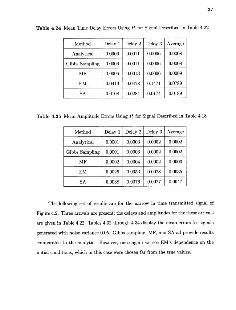
Table 4.24 Mean Time Delay Errors Using Pi for Signal Described in Table 4.22
Method Delay 1 Delay 2 Delay 3 Average
Analytical 0.0006 0.0011 0.0006 0.0008
Gibbs Sampling 0.0006 0.0011 0.0006 0.0008
MF 0.0006 0.0013 0.0006 0.0009
EM 0.0419 0.0478 0.1471 0.0789
SA 0.0108 0.0284 0.0174 0.0189
Table 4.25 Mean Amplitude Errors Using Pi for Signal Described in Table 4.18
Method Delay 1 Delay 2 Delay 3 Average
Analytical 0.0001 0.0003 0.0002 0.0002
Gibbs Sampling 0.0001 0.0003 0.0002 0.0002
MF 0.0002 0.0004 0.0002 0.0003
EM 0.0026 0.0053 0.0028 0.0035
SA 0.0038 0.0076 0.0027 0.0047
The following set of results are for the narrow in time transmitted signal of
Figure 4.2. Three arrivals are present; the delays and amplitudes for the these arrivals
are given in Table 4.22. Tables 4.32 through 4.34 display the mean errors for signals
generated with noise variance 0.05. Gibbs sampling, MF, and SA all provide results
comparable to the analytic. However, once again we see EM's dependence on the
initial conditions, which in this case were chosen far from the true values.
38
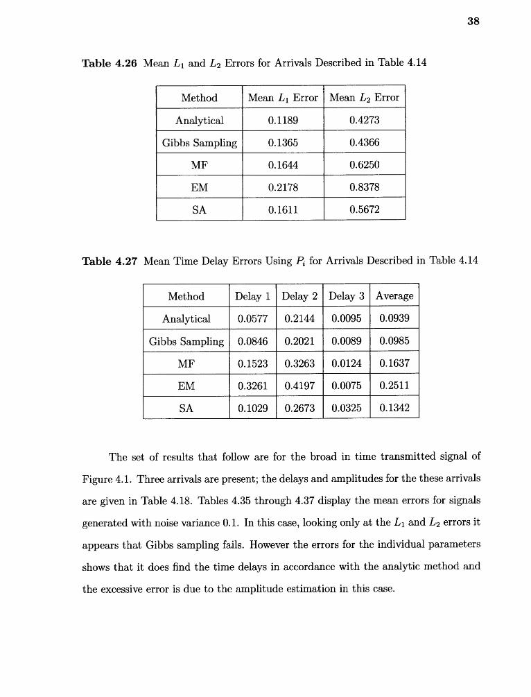
Table 4.26 Mean Lib and L2 Errors for Arrivals Described in Table 4.14
Method Mean Lib Error Mean L2 Error
Analytical 0.1189 0.4273
Gibbs Sampling 0.1365 0.4366
MF 0.1644 0.6250
EM 0.2178 0.8378
SA 0.1611 0.5672
Table 4.27 Mean Time Delay Errors Using Pn for Arrivals Described in Table 4.14
Method Delay 1 Delay 2 Delay 3 Average
Analytical 0.0577 0.2144 0.0095 0.0939
Gibbs Sampling 0.0846 0.2021 0.0089 0.0985
MF 0.1523 0.3263 0.0124 0.1637
EM 0.3261 0.4197 0.0075 0.2511
SA 0.1029 0.2673 0.0325 0.1342
The set of results that follow are for the broad in time transmitted signal of
Figure 4.1. Three arrivals are present; the delays and amplitudes for the these arrivals
are given in Table 4.18. Tables 4.35 through 4.37 display the mean errors for signals
generated with noise variance 0.1. In this case, looking only at the L ib and L2 errors it
appears that Gibbs sampling fails. However the errors for the individual parameters
shows that it does find the time delays in accordance with the analytic method and
the excessive error is due to the amplitude estimation in this case.
39
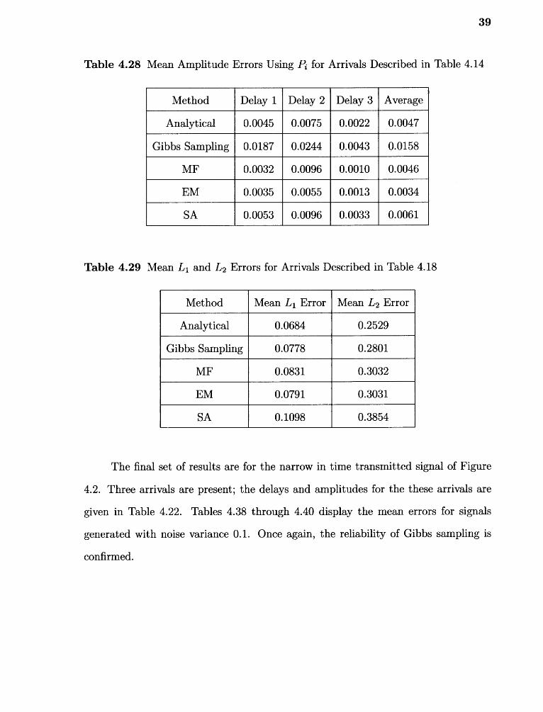
Table 4.28 Mean Amplitude Errors Using Pi for Arrivals Described in Table 4.14
Method Delay 1 Delay 2 Delay 3 Average
Analytical 0.0045 0.0075 0.0022 0.0047
Gibbs Sampling 0.0187 0.0244 0.0043 0.0158
MF 0.0032 0.0096 0.0010 0.0046
EM 0.0035 0.0055 0.0013 0.0034
SA 0.0053 0.0096 0.0033 0.0061
Table 4.29 Mean Lib and L2 Errors for Arrivals Described in Table 4.18
Method Mean Lib Error Mean L2 Error
Analytical 0.0684 0.2529
Gibbs Sampling 0.0778 0.2801
MF 0.0831 0.3032
EM 0.0791 0.3031
SA 0.1098 0.3854
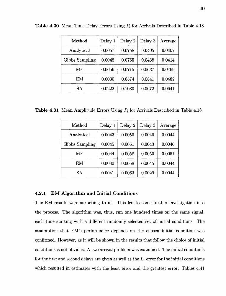
The final set of results are for the narrow in time transmitted signal of Figure
4.2. Three arrivals are present; the delays and amplitudes for the these arrivals are
given in Table 4.22. Tables 4.38 through 4.40 display the mean errors for signals
generated with noise variance 0.1. Once again, the reliability of Gibbs sampling is
confirmed.
40
Table 4.30 Mean Time Delay Errors Using Pi for Arrivals Described in Table 4.18
Method Delay 1 Delay 2 Delay 3 Average
Analytical 0.0057 0.0758 0.0405 0.0407
Gibbs Sampling 0.0048 0.0755 0.0438 0.0414
MF 0.0056 0.0715 0.0637 0.0469
EM 0.0030 0.0574 0.0841 0.0482
SA 0.0222 0.1030 0.0672 0.0641
Table 4.31 Mean Amplitude Errors Using Pi for Arrivals Described in Table 4.18
Method Delay 1 Delay 2 Delay 3 Average
Analytical 0.0043 0.0050 0.0040 0.0044
Gibbs Sampling 0.0045 0.0051 0.0043 0.0046
MF 0.0044 0.0058 0.0050 0.0051
EM 0.0030 0.0058 0.0045 0.0044
SA 0.0041 0.0063 0.0029 0.0044
4.2.1 EM Algorithm and Initial Conditions
The EM results were surprising to us. This led to some further investigation into
the process. The algorithm was, thus, run one hundred times on the same signal,
each time starting with a different randomly selected set of initial conditions. The
assumption that EM's performance depends on the chosen initial condition was
confirmed. However, as it will be shown in the results that follow the choice of initial
conditions is not obvious. A two arrival problem was examined. The initial conditions
for the first and second delays are given as well as the L i error for the initial conditions
which resulted in estimates with the least error and the greatest error. Tables 4.41
41
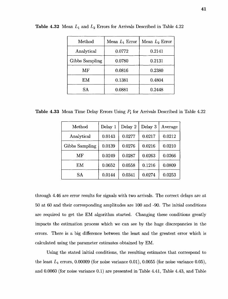
Table 4.32 Mean L i and L2 Errors for Arrivals Described in Table 4.22
Method Mean L i Error Mean L2 Error
Analytical 0.0772 0.2141
Gibbs Sampling 0.0780 0.2131
MF 0.0816 0.2380
EM 0.1381 0.4804
SA 0.0881 0.2448
Table 4.33 Mean Time Delay Errors Using Pn for Arrivals Described in Table 4.22
Method Delay 1 Delay 2 Delay 3 Average
Analytical 0.0143 0.0277 0.0217 0.0212
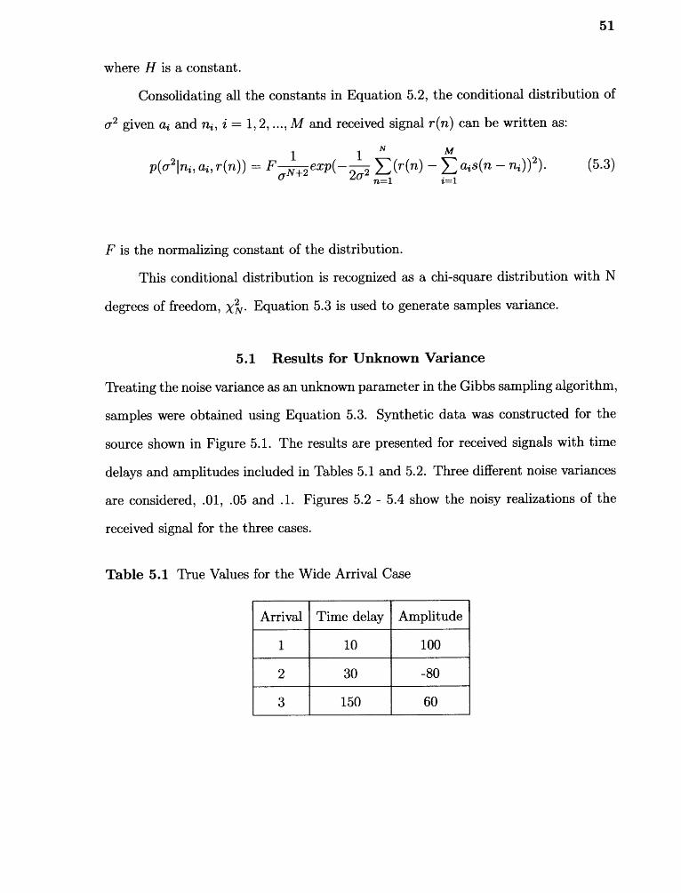
Gibbs Sampling 0.0139 0.0276 0.0216 0.0210
MF 0.0249 0.0287 0.0263 0.0266
EM 0.0652 0.0558 0.1216 0.0809
SA 0.0144 0.0341 0.0274 0.0253
through 4.46 are error results for signals with two arrivals. The correct delays are at
50 at 60 and their corresponding amplitudes are 100 and -90. The initial conditions
are required to get the EM algorithm started. Changing these conditions greatly
impacts the estimation process which we can see by the huge discrepancies in the
errors. There is a big difference between the least and the greatest error which is
calculated using the parameter estimates obtained by EM.
Using the stated initial conditions, the resulting estimates that correspond to
the least L i errors, 0.00009 (for noise variance 0.01), 0.0055 (for noise variance 0.05),
and 0.0060 (for noise variance 0.1) are presented in Table 4.41, Table 4.43, and Table
42
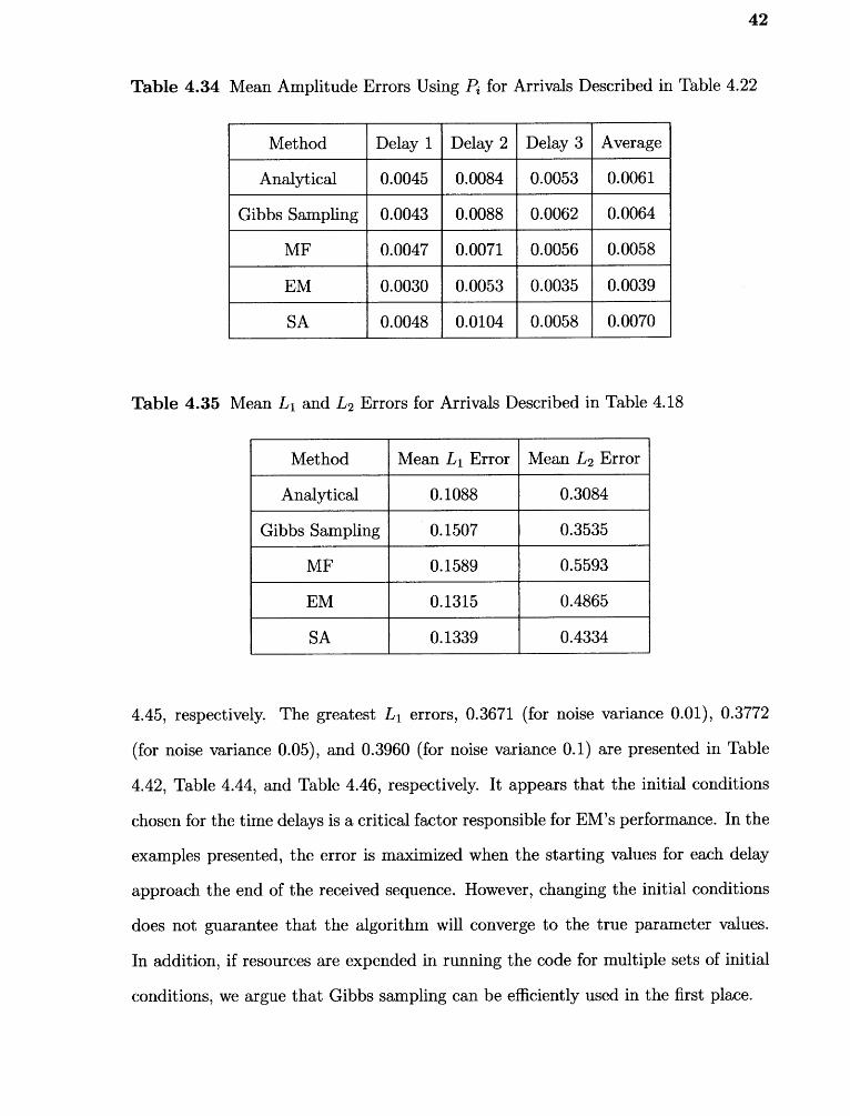
Table 4.34 Mean Amplitude Errors Using Pi for Arrivals Described in Table 4.22
Method Delay 1 Delay 2 Delay 3 Average
Analytical 0.0045 0.0084 0.0053 0.0061
Gibbs Sampling 0.0043 0.0088 0.0062 0.0064
MF 0.0047 0.0071 0.0056 0.0058
EM 0.0030 0.0053 0.0035 0.0039
SA 0.0048 0.0104 0.0058 0.0070
Table 4.35 Mean Lib and L2 Errors for Arrivals Described in Table 4.18
Method Mean Lib Error Mean L2 Error
Analytical 0.1088 0.3084
Gibbs Sampling 0.1507 0.3535
MF 0.1589 0.5593
EM 0.1315 0.4865
SA 0.1339 0.4334
4.45, respectively. The greatest L ib errors, 0.3671 (for noise variance 0.01), 0.3772
(for noise variance 0.05), and 0.3960 (for noise variance 0.1) are presented in Table
4.42, Table 4.44, and Table 4.46, respectively. It appears that the initial conditions
chosen for the time delays is a critical factor responsible for EM's performance. In the
examples presented, the error is maximized when the starting values for each delay
approach the end of the received sequence. However, changing the initial conditions
does not guarantee that the algorithm will converge to the true parameter values.
In addition, if resources are expended in running the code for multiple sets of initial
conditions, we argue that Gibbs sampling can be efficiently used in the first place.
43
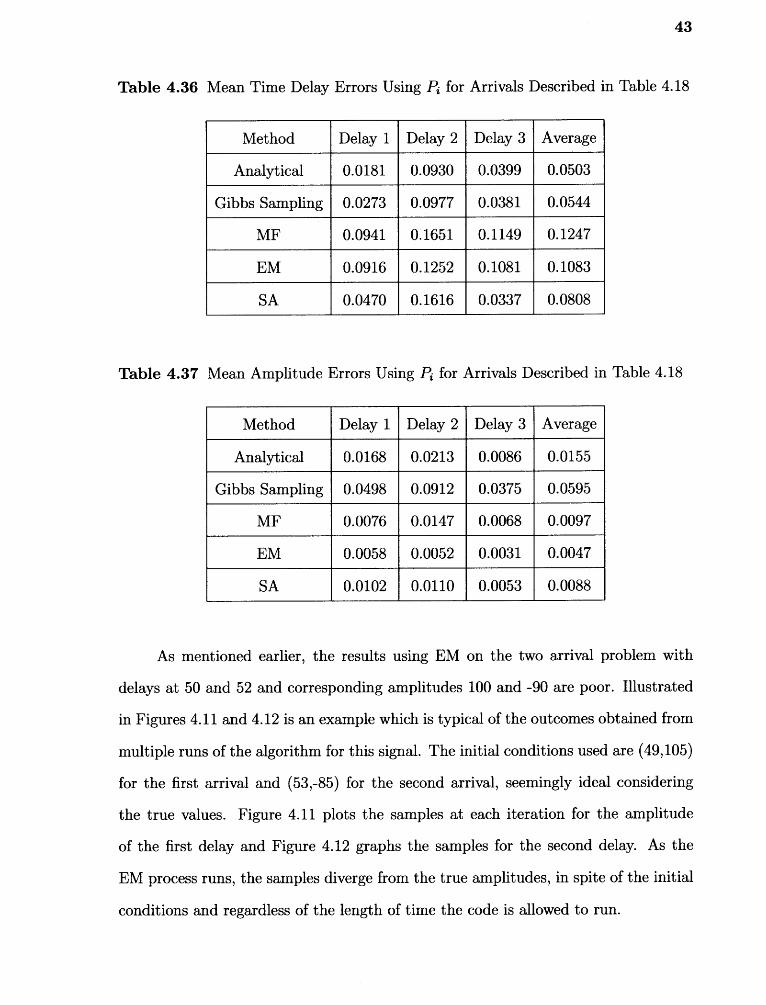
Table 4.36 Mean Time Delay Errors Using Pn for Arrivals Described in Table 4.18
Method Delay 1 Delay 2 Delay 3 Average
Analytical 0.0181 0.0930 0.0399 0.0503
Gibbs Sampling 0.0273 0.0977 0.0381 0.0544
MF 0.0941 0.1651 0.1149 0.1247
EM 0.0916 0.1252 0.1081 0.1083
SA 0.0470 0.1616 0.0337 0.0808
Table 4.37 Mean Amplitude Errors Using Pn for Arrivals Described in Table 4.18
Method Delay 1 Delay 2 Delay 3 Average
Analytical 0.0168 0.0213 0.0086 0.0155
Gibbs Sampling 0.0498 0.0912 0.0375 0.0595
MF 0.0076 0.0147 0.0068 0.0097
EM 0.0058 0.0052 0.0031 0.0047
SA 0.0102 0.0110 0.0053 0.0088
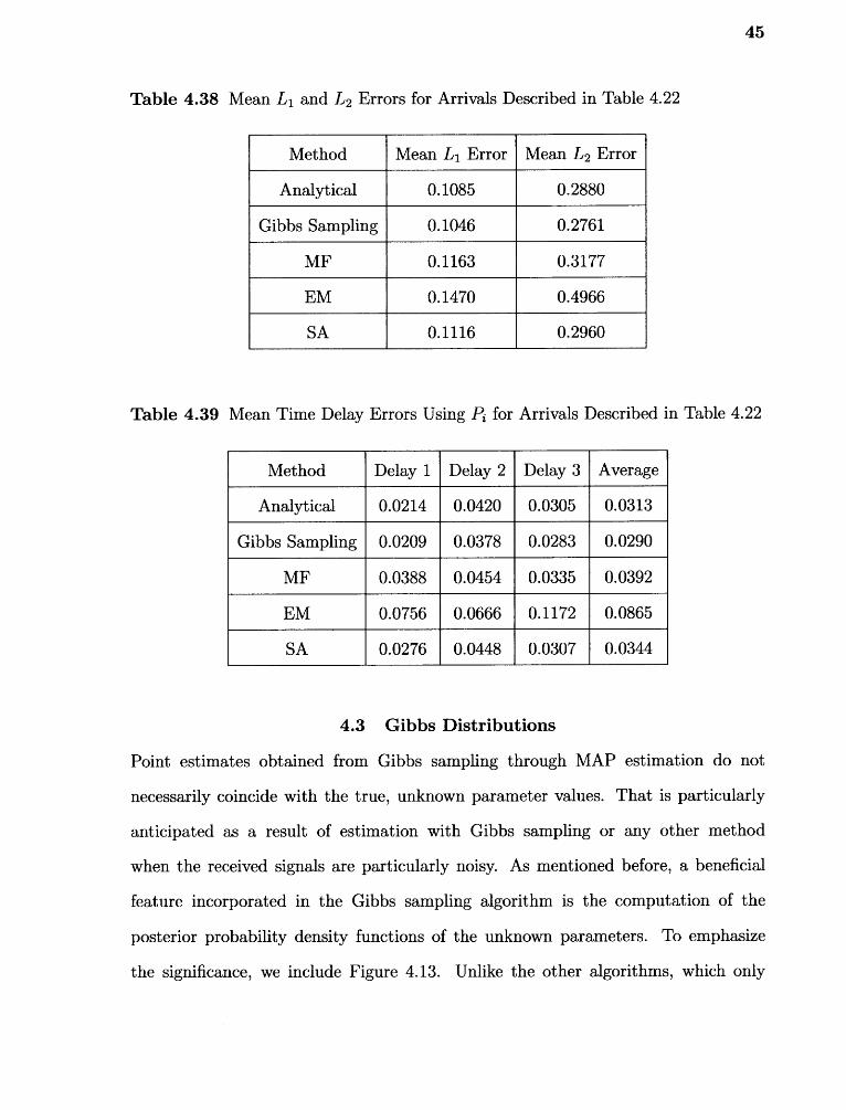
As mentioned earlier, the results using EM on the two arrival problem with
delays at 50 and 52 and corresponding amplitudes 100 and -90 are poor. Illustrated
in Figures 4.11 and 4.12 is an example which is typical of the outcomes obtained from
multiple runs of the algorithm for this signal. The initial conditions used are (49,105)
for the first arrival and (53,-85) for the second arrival, seemingly ideal considering
the true values. Figure 4.11 plots the samples at each iteration for the amplitude
of the first delay and Figure 4.12 graphs the samples for the second delay. As the
EM process runs, the samples diverge from the true amplitudes, in spite of the initial
conditions and regardless of the length of time the code is allowed to run.
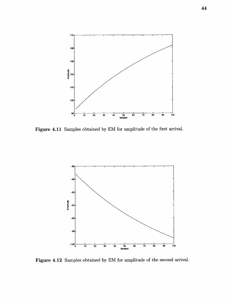
Figure 4.11 Samples obtained by EM for amplitude of the first arrival.
Figure 4.12 Samples obtained by EM for amplitude of the second arrival.
44
45
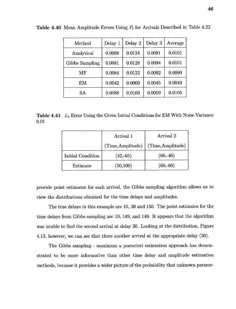
Table 4.38 Mean L1 and L2 Errors for Arrivals Described in Table 4.22
Method Mean Li Error Mean L2 Error
Analytical 0.1085 0.2880
Gibbs Sampling 0.1046 0.2761
MF 0.1163 0.3177
EM 0.1470 0.4966
SA 0.1116 0.2960
Table 4.39 Mean Time Delay Errors Using Pi for Arrivals Described in Table 4.22
Method Delay 1 Delay 2 Delay 3 Average
Analytical 0.0214 0.0420 0.0305 0.0313
Gibbs Sampling 0.0209 0.0378 0.0283 0.0290
MF 0.0388 0.0454 0.0335 0.0392
EM 0.0756 0.0666 0.1172 0.0865
SA 0.0276 0.0448 0.0307 0.0344
4.3 Gibbs Distributions
Point estimates obtained from Gibbs sampling through MAP estimation do not
necessarily coincide with the true, unknown parameter values. That is particularly
anticipated as a result of estimation with Gibbs sampling or any other method
when the received signals are particularly noisy. As mentioned before, a beneficial
feature incorporated in the Gibbs sampling algorithm is the computation of the
posterior probability density functions of the unknown parameters. To emphasize
the significance, we include Figure 4.13. Unlike the other algorithms, which only
46
Table 4.40 Mean Amplitude Errors Using Pn for Arrivals Described in Table 4.22
Method Delay 1 Delay 2 Delay 3 Average
Analytical 0.0088 0.0124 0.0091 0.0101
Gibbs Sampling 0.0081 0.0128 0.0094 0.0101
MF 0.0084 0.0122 0.0092 0.0099
EM 0.0042 0.0060 0.0045 0.0049
SA 0.0088 0.0169 0.0059 0.0105
Table 4.41 L i Error Using the Given Initial Conditions for EM With Noise Variance0.01
Arrival 1
(Time,Amplitude)
Arrival 2
(Time,Amplitude)
Initial Condition (42,-65) (66,-46)
Estimate (50,100) (60,-80)
provide point estimates for each arrival, the Gibbs sampling algorithm allows us to
view the distributions obtained for the time delays and amplitudes.
The true delays in this example are 10, 30 and 150. The point estimates for the
time delays from Gibbs sampling are 10, 149, and 149. It appears that the algorithm
was unable to find the second arrival at delay 30. Looking at the distribution, Figure
4.13, however, we can see that there another arrival at the appropriate delay (30).
The Gibbs sampling - maximum a posteriori estimation approach has demon-
strated to be more informative than other time delay and amplitude estimation
methods, because it provides a wider picture of the probability that unknown parame-
47
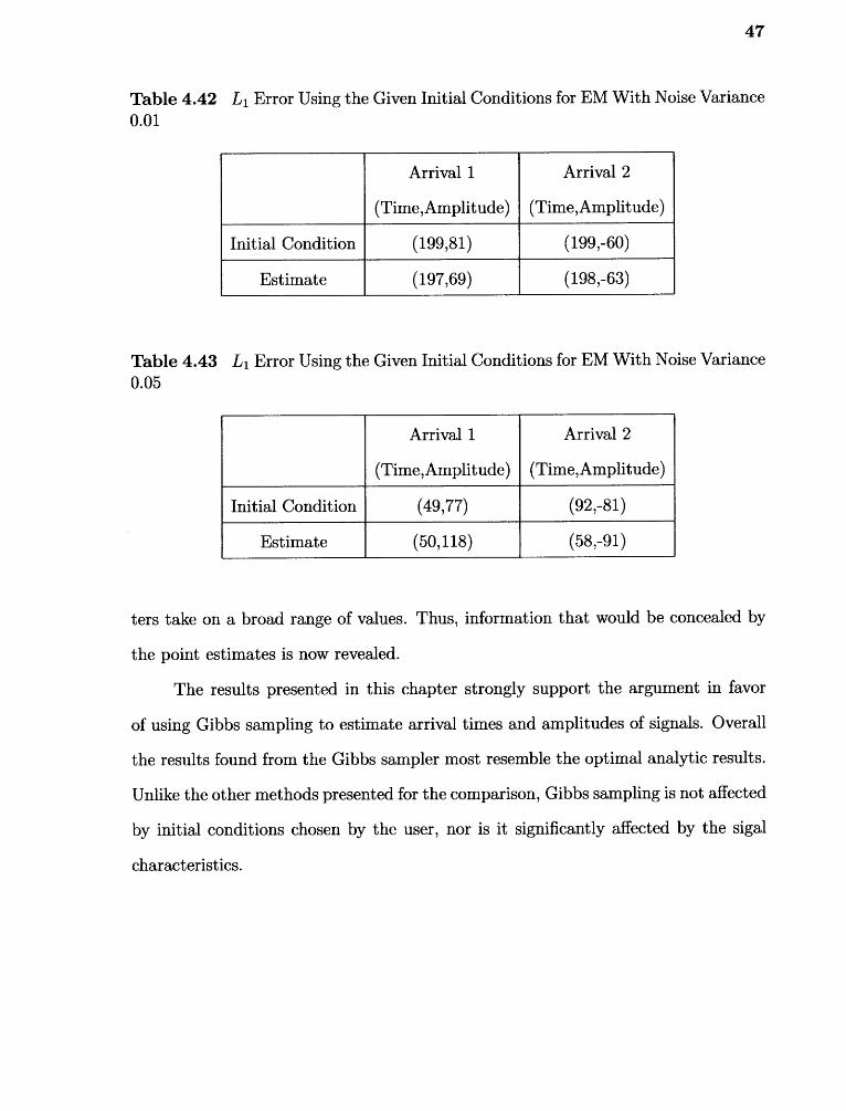
Table 4.42 L i Error Using the Given Initial Conditions for EM With Noise Variance0.01
Arrival 1
(Time,Amplitude)
Arrival 2
(Time,Amplitude)
Initial Condition (199,81) (199,-60)
Estimate (197,69) (198,-63)
Table 4.43 L i Error Using the Given Initial Conditions for EM With Noise Variance0.05
Arrival 1
(Time,Amplitude)
Arrival 2
(Time,Amplitude)
Initial Condition (49,77) (92,-81)
Estimate (50,118) (58,-91)
ters take on a broad range of values. Thus, information that would be concealed by
the point estimates is now revealed.
The results presented in this chapter strongly support the argument in favor
of using Gibbs sampling to estimate arrival times and amplitudes of signals. Overall
the results found from the Gibbs sampler most resemble the optimal analytic results.
Unlike the other methods presented for the comparison, Gibbs sampling is not affected
by initial conditions chosen by the user, nor is it significantly affected by the sigal
characteristics.
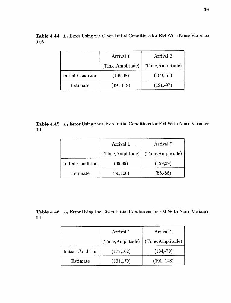
48
Table 4.44 Lib Error Using the Given Initial Conditions for EM With Noise Variance0.05
Arrival 1
(Time,Amplitude)
Arrival 2
(Time,Amplitude)
Initial Condition (199,98) (199,-51)
Estimate (191,119) (191,-97)
Table 4.45 Lib Error Using the Given Initial Conditions for EM With Noise Variance0.1
Arrival 1
(Time,Amplitude)
Arrival 2
(Time,Amplitude)
Initial Condition (39,89) (129,39)
Estimate (50,120) (58,-88)
Table 4.46 Lib Error Using the Given Initial Conditions for EM With Noise Variance0.1
Arrival 1
(Time,Amplitude)
Arrival 2
(Time,Amplitude)
Initial Condition (177,102) (184,-79)
Estimate (191,179) (191,-148)
500
-o2 0E
-500
5500
5000
500
0
-500
-5000
-550050 500 550 200
Time Delay
5500
1000
500
0
-500
-5000
550050 500 550 200
Time Delay
50 500 550 200
Time Delay
1500
5000
-5000
-5500
49
Figure 4.13 Distributions obtained by Gibbs sampling.
CHAPTER 5
MODELLING VARIANCE AS AN UNKNOWN PARAMETER
Recall that the received signal follows Equation (1.1). We have shown that the Gibbs
sampler successfully identified the amplitudes and time delays assuming the noise
variance was known. This variance is now treated as an unknown parameter, added
to the attenuated and delayed replicas of the transmitted signal. To do this, we make
use of the following theorem:
Thm.: Let the sample quantity N s2be distributed as (o-2/N)A. If the prior
distribution of logo is locally uniform, then, given Ns2, K2 is distributed a posteriori as
(As2 )xA. ,-2 [34].
In the context of the work presented here, x2N is the sum of the squares of A
random numbers. A is the length of the received signal and Nsy = ET,=i (r(n) —
E im=i ais(n — ni))2
We will use the following noninformative prior for the variance [30, 34].
/ 2\ = 1 y' CI
2 > 0 (5.1)
This choice represents the fact that no information is available on the variance.
Including this in the joint distribution Equation 3.5, we can now write the posterior
probability distribution function of all unknown parameters (in this case, n i , ail for
i = 1, , M, and cry) as follows:
p(ni, ...,nm,ai, am, 0-y Ir(n)) =1 1
H m y
1
(Or)o
Koexp(
1 > (ran) — ais(n — ni))2 ), (5.2)A A- 2A-y n=1 i=1
50
51
where H is a constant.
Consolidating all the constants in Equation 5.2, the conditional distribution of
A-2 given ail and ni, i = 1, 2, ..., M and received signal r(n) can be written as:
p(K y In i , ail, r(n)) = FK
lo+y exP( — -2,2 E ( ( ) - E ajs(n — n n )) y )•
F is the normalizing constant of the distribution.
This conditional distribution is recognized as a chi-square distribution with N
degrees of freedom, x2N. Equation 5.3 is used to generate samples variance.
5.1 Results for Unknown Variance
Treating the noise variance as an unknown parameter in the Gibbs sampling algorithm,
samples were obtained using Equation 5.3. Synthetic data was constructed for the
source shown in Figure 5.1. The results are presented for received signals with time
delays and amplitudes included in Tables 5.1 and 5.2. Three different noise variances
are considered, .01, .05 and .1. Figures 5.2 - 5.4 show the noisy realizations of the
received signal for the three cases.
Table 5.1 True Values for the Wide Arrival Case
Arrival Time delay Amplitude
1 10 100
2 30 -80
3 150 60
1 N m
(5.3)n=1 i=1
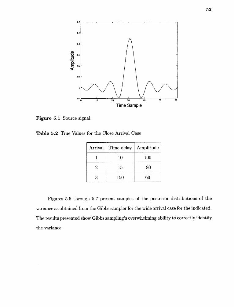
52
150 2o 30 40 50 60
Time Sample
Figure 5.1 Source signal.
Table 5.2 True Values for the Close Arrival Case
Arrival Time delay Amplitude
1 10 100
2 15 -80
3 150 60
Figures 5.5 through 5.7 present samples of the posterior distributions of the
variance as obtained from the Gibbs sampler for the wide arrival case for the indicated.
The results presented show Gibbs sampling's overwhelming ability to correctly identify
the variance.
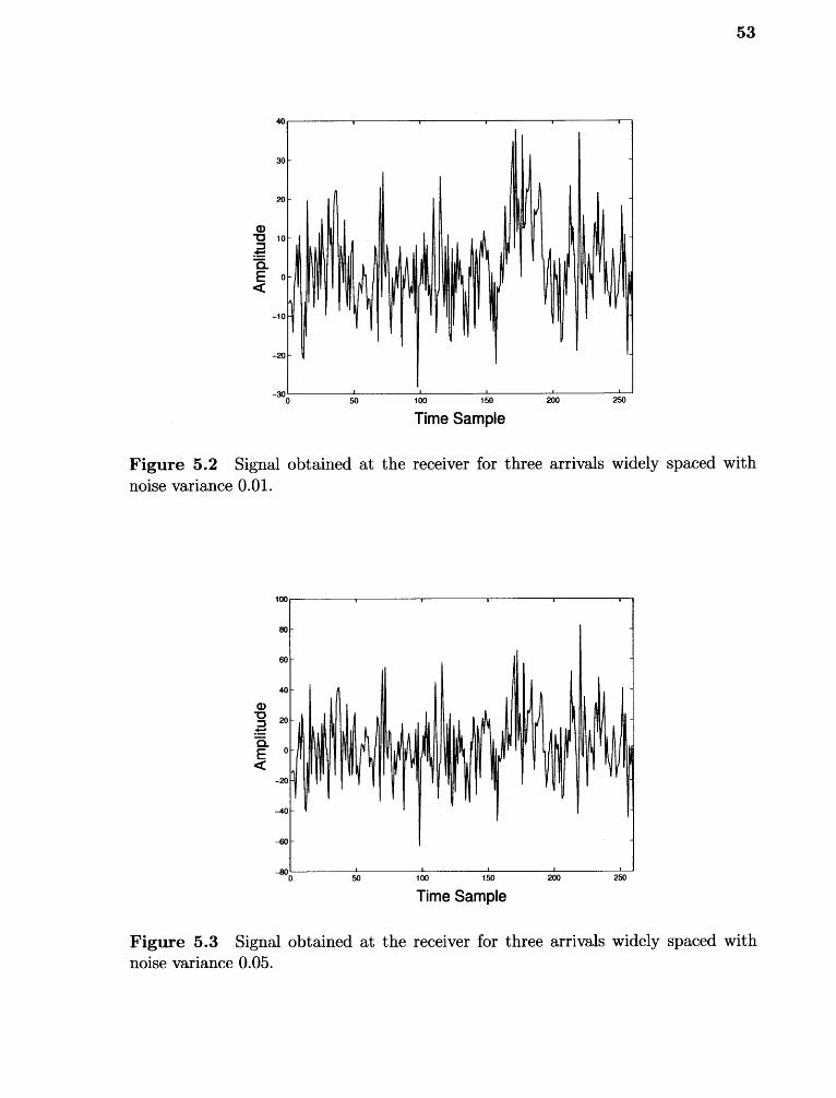
a)0
a..
_ 0
53
50 ii;i3 50Time Sample
200 250
Figure 5.2 Signal obtained at the receiver for three arrivals widely spaced withnoise variance 0.01.
a)
a_E
Time Sample
Figure 5.3 Signal obtained at the receiver for three arrivals widely spaced withnoise variance 0.05.
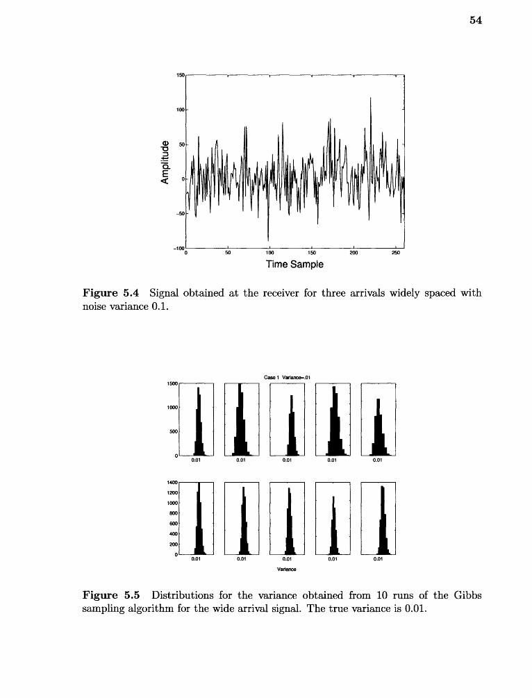
54
150
100 -
ap
E
pi
-100 0 50 100 150 200 250
Time Sample
Figure 5.4 Signal obtained at the receiver for three arrivals widely spaced withnoise variance 0.1.
Case 1 Variance= 051500
1000
500
0 0.05
0.05
0.05
0.05
0.05
1400
1290
1000
800
600
400
290
0 0.05
0.05
0.05
0.05
0.05
Variance
Figure 5.5 Distributions for the variance obtained from 10 runs of the Gibbssampling algorithm for the wide arrival signal. The true variance is 0.01.
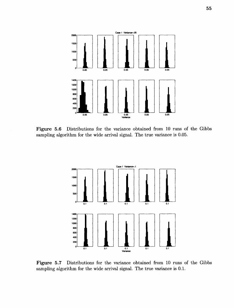
2000
5500
5000
500
00.05 0.050.050.050.05
0.050.05 0.050.05
5400
1200
5000
800
600
400
200
00.05
Variance
2000
5500
5000
500
00. 1 0. 1 0.1 0. 1 0. 1
Case 5 Variance
55
Figure 5.6 Distributions for the variance obtained from 10 runs of the Gibbssampling algorithm for the wide arrival signal. The true variance is 0.05.
Case 5 Veriance..1
54001200
5000
800
600
400
200
00.1
0.1
0.1
0. 1
0. 1Variance
Figure 5.7 Distributions for the variance obtained from 10 runs of the Gibbssampling algorithm for the wide arrival signal. The true variance is 0.1.
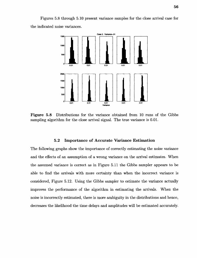
0.050.05 0.050.05
1500
1000
500
0
2000
1500
1000
500
0
10.05
56
Figures 5.8 through 5.10 present variance samples for the close arrival case for
the indicated noise variances.
Case 2. Variance..01
0.05
0.05
0.05
0.05
0.05Variance
Figure 5.8 Distributions for the variance obtained from 10 runs of the Gibbssampling algorithm for the close arrival signal. The true variance is 0.01.
5.2 Importance of Accurate Variance Estimation
The following graphs show the importance of correctly estimating the noise variance
and the effects of an assumption of a wrong variance on the arrival estimates. When
the assumed variance is correct as in Figure 5.11 the Gibbs sampler appears to be
able to find the arrivals with more certainty than when the incorrect variance is
considered, Figure 5.12. Using the Gibbs sampler to estimate the variance actually
improves the performance of the algorithm in estimating the arrivals. When the
noise is incorrectly estimated, there is more ambiguity in the distributions and hence,
decreases the likelihood the time delays and amplitudes will be estimated accurately.
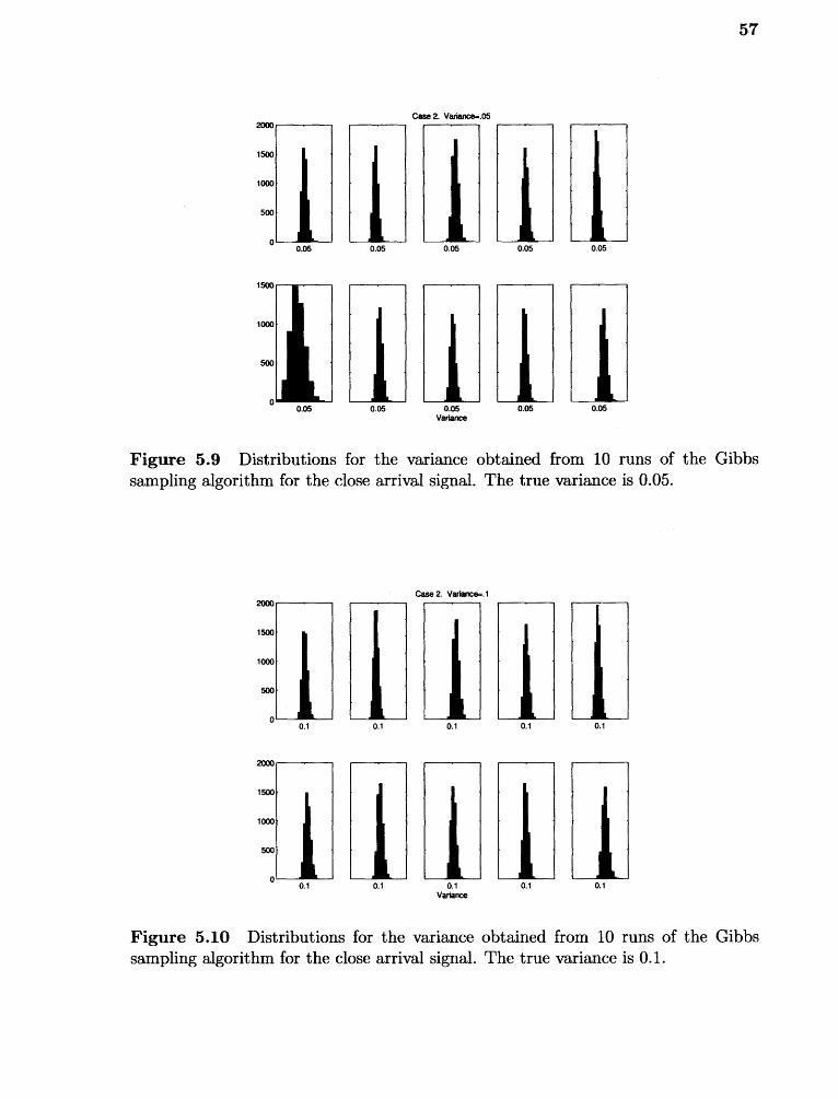
0.1
0.1Variance
2900
1500
1000
500
0
1500
1000
500
0
0.05
0.1
0.05
0.1
0.05
0.05
0.1
0.1
2900
1500
1000
500
00.10.10.1 0.10.1
Case 2. Variance=.1
57
Figure 5.9 Distributions for the variance obtained from 10 runs of the Gibbssampling algorithm for the close arrival signal. The true variance is 0.05.
Case 2. Variance
2900
1500
1000
500
0 0.1
0.1
0.1
0.1
0.1Variance
Figure 5.10 Distributions for the variance obtained from 10 runs of the Gibbssampling algorithm for the close arrival signal. The true variance is 0.1.
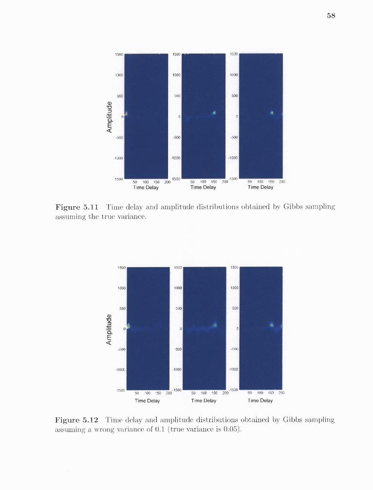
50 100 150
Time Delay
1500
1000
500
0
-500
-1000
-1500200 50 100 150 200
Time Delay
1500
1000
500
-500
-1000
1- 50050 100 150 200Time Delay
-1500
1500
1000
500
-500
-1000
1500
1000
500
-500
-1000
-1500
1500
1- 50050 100 150 200
Time Delay
-500
-1000
1- 50050 100 150 200
Time Delay
1500
1000
500
0
1000
500
0
-500
-1000
50 100 150 200
Time Delay
Figure 5.11 Time delay and amplitude distributions obtained by Gibbs samplingassuming the true variance.
58
Figure 5.12 Time delay and amplitude distributions obtained by Gibbs samplingassuming a wrong variance of 0.1 (true variance is 0.05).
CHAPTER 6
UNKNOWN NUMBER OF ARRIVALS
We have assumed until now that the number of arrivals in the received signal is
known. This assumption is quite common [17, 351]. It is argued that this is not as
restrictive as it appears since, in many cases the number of paths (arrivals) can be
determined from the geometry of the channel. However, since we do not assume any
prior knowledge about the environment, it is not valid to assume prior knowledge
about the number of arrivals. Therefore, the next task at hand is to use the Gibbs
sampling algorithm to determine the number of arrivals present in the received signal.
6.1 Empirical Approach
First, we run the Gibbs sampling algorithm assuming present in the received signal
are two arrivals, three arrivals, four arrivals, etc. One interesting feature of the Gibbs
sampler is that, when generating samples for the time delays, the program can be
forced to find an arrival different from those already found. When running the Gibbs
sampler assuming the number of arrivals is greater than the true number of arrivals,
the process often gets "stuck" in a loop. This is the first indication that the original
guess exceeds the true number of arrivals and provides a limit on the maximum
number of arrivals that should be assumed when running the algorithm. Exploiting
this phenomenon, we can implement a flag waving technique suggesting that it may
be necessary to reduce the assumed number of arrivals.
Furthermore, we can study the distributions obtained for each considered case.
In the next example, the true number of arrivals is three. The received time-series
is generated employing the source signal of Figure 6.1 with various amplitudes, time
delays, and added noise.
59
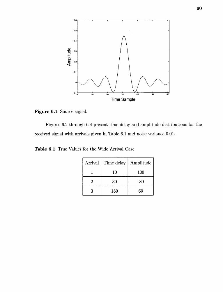
60
Time Sample
Figure 6.1 Source signal.
Figures 6.2 through 6.4 present time delay and amplitude distributions for the
received signal with arrivals given in Table 6.1 and noise variance 0.01.
Table 6.1 True Values for the Wide Arrival Case
Arrival Time delay Amplitude
1 10 100
2 30 -80
3 150 60
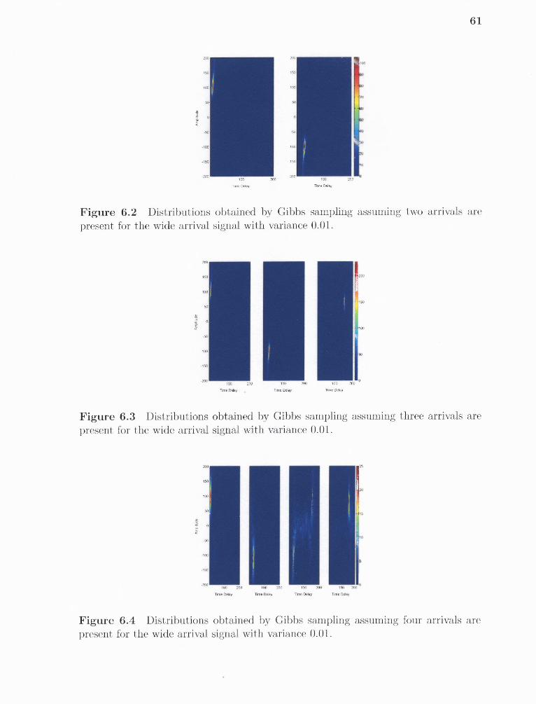
61
200
050
000
50
100
050
000
50
0
-150
-000
-050
-100
-150
0
-000
-050
-200000Time Delay
200
-000
-050
-100
200
050100
50
0
_200
200200100
Time Delay Time Delay
000
Time Delay
-050
-000
-050
-200100 200
Time Delay Time Delay
200
050
100
050
Figure 6.2 Distributions obtained by Gibbs sampling assuming two arrivals arepresent for the wide arrival signal with variance 0.01.
Figure 6.3 Distributions obtained by Gibbs sampling assuming three arrivals arepresent for the wide arrival signal with variance 0.01.
Figure 6.4 Distributions obtained by Gibbs sampling assuming four arrivals arepresent for the wide arrival signal with variance 0.01.
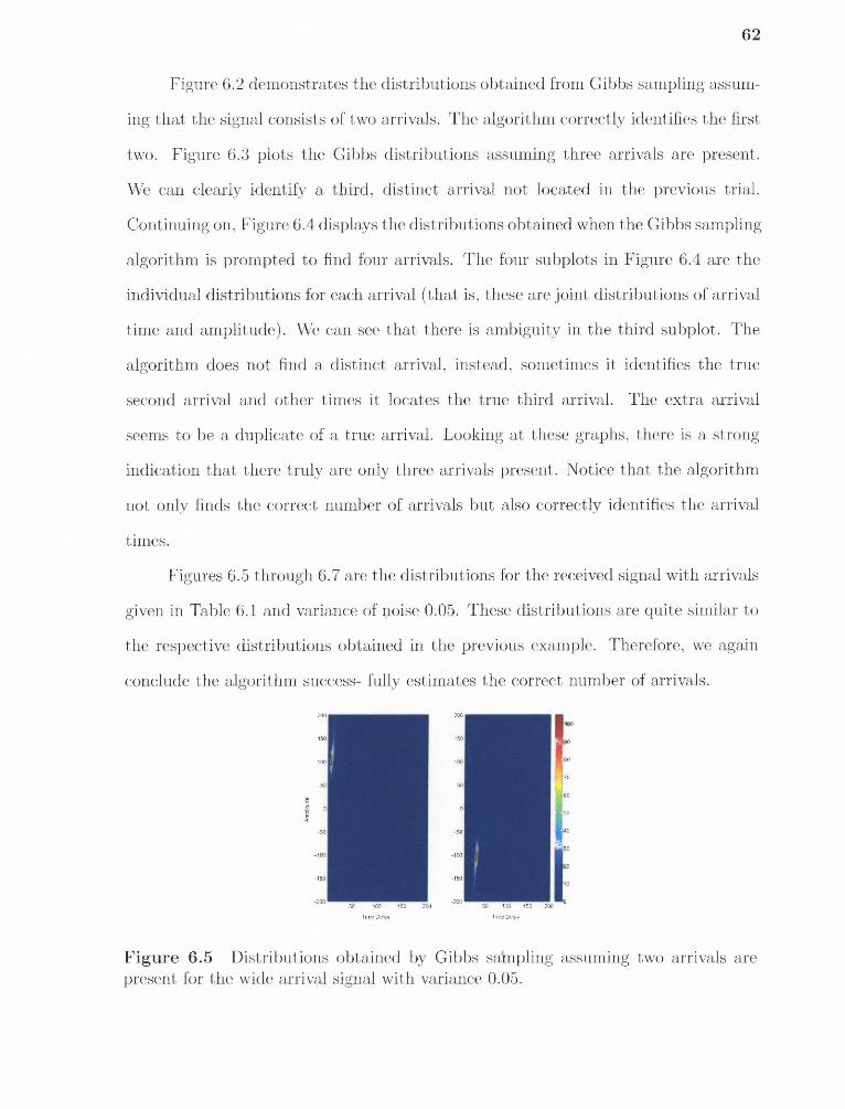
Time Delay
62
Figure 6.2 demonstrates the distributions obtained from Gibbs sampling assum-
ing that the signal consists of two arrivals. The algorithm correctly identifies the first
two. Figure 6.3 plots the Gibbs distributions assuming three arrivals are present.
We can clearly identify a third, distinct arrival not located in the previous trial.
Continuing on, Figure 6.4 displays the distributions obtained when the Gibbs sampling
algorithm is prompted to find four arrivals. The four subplots in Figure 6.4 are the
individual distributions for each arrival (that is, these are joint distributions of arrival
time and amplitude). We can see that there is ambiguity in the third subplot. The
algorithm does not find a distinct arrival, instead, sometimes it identifies the true
second arrival and other times it locates the true third arrival. The extra arrival
seems to be a duplicate of a true arrival. Looking at these graphs, there is a strong
indication that there truly are only three arrivals present. Notice that the algorithm
not only finds the correct number of arrivals but also correctly identifies the arrival
times.
Figures 6.5 through 6.7 are the distributions for the received signal with arrivals
given in Table 6.1 and variance of noise 0.05. These distributions are quite similar to
the respective distributions obtained in the previous example. Therefore, we again
conclude the algorithm success- fully estimates the correct number of arrivals.
Figure 6.5 Distributions obtained by Gibbs sampling assuming two arrivals arepresent for the wide arrival signal with variance 0.05.
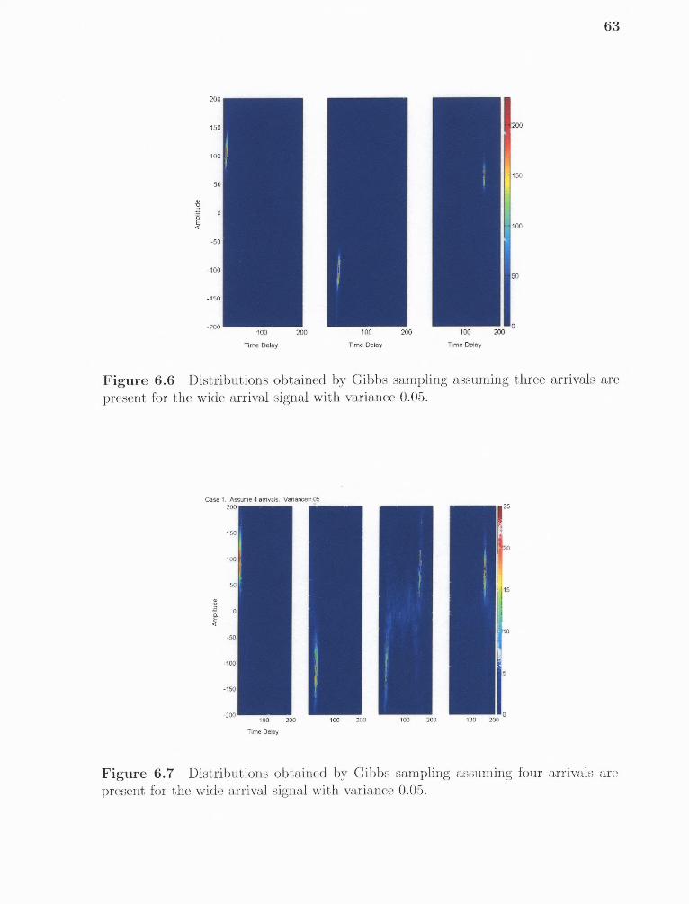
200
150
100
50
200
150
-A
0o.E 100
-50
-100
-150
-200
50
100 200100 200
Time Delay
0100 200
Time DelayTime Delay
63
Case 1. Assume 4 arrivals. Variance=0520
-200100 200 100 200 100 200
15C(
10C
15C
-150
-10C
-150
Figure 6.6 Distributions obtained by Gibbs sampling assuming three arrivals arepresent for the wide arrival signal with variance 0.05.
Time Delay
Figure 6.7 Distributions obtained by Gibbs sampling assuming four arrivals arepresent for the wide arrival signal with variance 0.05.
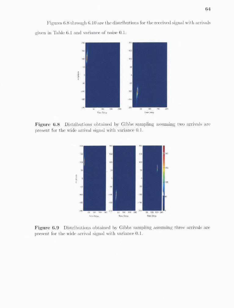
50 100 150
Time Delay
-100
-150
-20
100
150
-50
50
)0
200
-200 -100 -200 050 100 150 200 50 100 150 100 50 100 150 100
100
150
100
50
200
150
100
50
-50
-100
-150
10f
150(
10(
100
150150
50 150
0
-5(
-10(
- 15(
0
-50
-100
-150
64
Figures 6.8 through 6.10 are the distributions for the received signal with arrivals
given in Table 6.1 and variance of noise 0.1.
100
150
100
50
-50
-100
-150
-10050 100 150
100
Time Delay
Figure 6.8 Distributions obtained by Gibbs sampling assuming two arrivals arepresent for the wide arrival signal with variance 0.1.
Time Delay Time Delay Time Delay
Figure 6.9 Distributions obtained by Gibbs sampling assuming three arrivals arepresent for the wide arrival signal with variance 0.1.
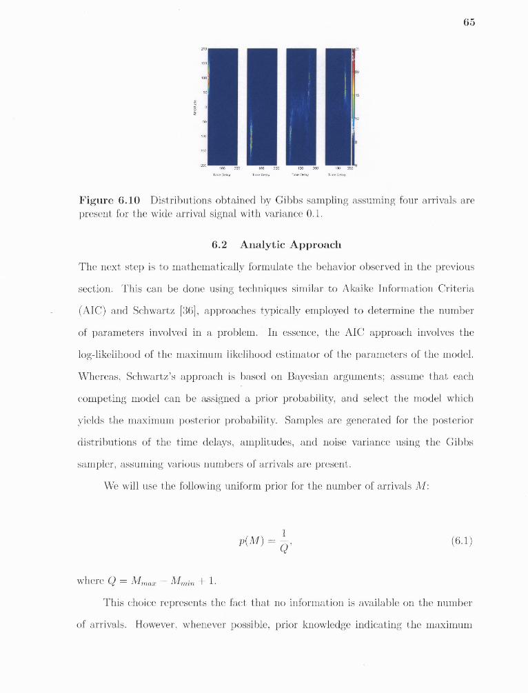
200
050
100
65
50
5
-50
-100
-150
-200 000 200
100 100
000 200
100 200
Time Delay
Time Del,
Time Delay
Time Delay
Figure 6.10 Distributions obtained by Gibbs sampling assuming four arrivals arepresent for the wide arrival signal with variance 0.1.
6.2 Analytic Approach
The next step is to mathematically formulate the behavior observed in the previous
section. This can be done using techniques similar to Akaike Information Criteria
(AIC) and Schwartz [36], approaches typically employed to determine the number
of parameters involved in a problem. In essence, the AIC approach involves the
log-likelihood of the maximum likelihood estimator of the parameters of the model.
Whereas, Schwartz's approach is based on Bayesian arguments; assume that each
competing model can be assigned a prior probability, and select the model which
yields the maximum posterior probability. Samples are generated for the posterior
distributions of the time delays, amplitudes, and noise variance using the Gibbs
sampler, assuming various numbers of arrivals are present.
We will use the following uniform prior for the number of arrivals M:
(6.1)
where Q = 114-— max — Mmnn + 1 .
This choice represents the fact that no information is available on the number
of arrivals. However, whenever possible, prior knowledge indicating the maximum
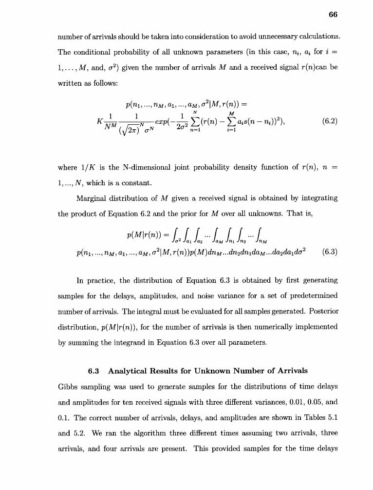
66
number of arrivals should be taken into consideration to avoid unnecessary calculations.
The conditional probability of all unknown parameters (in this case, n i , ai for i =
, M, and, Ay ) given the number of arrivals M and a received signal r(n)can be
written as follows:
p(n1 , ...,Om , al , ..., am , cry lM,r(n)) =1 1 1
N M
K o exp(— ,.Cy E (r(n) — E ais(n — ni))2),Amp (V27)
or o L u i=1 i=1
(6.2)
where 1/K is the N-dimensional joint probability density function of r(n), n =
1, A, which is a constant.
Marginal distribution of M given a received signal is obtained by integrating
the product of Equation 6.2 and the prior for M over all unknowns. That is,
P(mIr (n)) = L2 al fa2 Jam Li L2 iM
P(ni, nm,ai, ..., aMI, Ky1M, r (n))p(M)dnm...dnydnidam ...daydaidA-2 (6.3)
In practice, the distribution of Equation 6.3 is obtained by first generating
samples for the delays, amplitudes, and noise variance for a set of predetermined
number of arrivals. The integral must be evaluated for all samples generated. Posterior
distribution, p(Mir (n)), for the number of arrivals is then numerically implemented
by summing the integrand in Equation 6.3 over all parameters.
6.3 Analytical Results for Unknown Number of Arrivals
Gibbs sampling was used to generate samples for the distributions of time delays
and amplitudes for ten received signals with three different variances, 0.01, 0.05, and
0.1. The correct number of arrivals, delays, and amplitudes are shown in Tables 5.1
and 5.2. We ran the algorithm three different times assuming two arrivals, three
arrivals, and four arrivals are present. This provided samples for the time delays
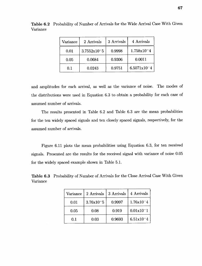
67
Table 6.2 Probability of Number of Arrivals for the Wide Arrival Case With GivenVariance
Variance 2 Arrivals 3 Arrivals 4 Arrivals
0.01 3.7552x10- 5 0.9998 1.758x10⁻⁴
0.05 0.0684 0.9306 0.0011
0.1 0.0243 0.9751 6.5071x10⁻⁴
and amplitudes for each arrival, as well as the variance of noise. The modes of
the distributions were used in Equation 6.3 to obtain a probability for each case of
assumed number of arrivals.
The results presented in Table 6.2 and Table 6.3 are the mean probabilities
for the ten widely spaced signals and ten closely spaced signals, respectively, for the
assumed number of arrivals.
Figure 6.11 plots the mean probabilities using Equation 6.3, for ten received
signals. Presented are the results for the received signal with variance of noise 0.05
for the widely spaced example shown in Table 5.1.
Table 6.3 Probability of Number of Arrivals for the Close Arrival Case With GivenVariance
Variance 2 Arrivals 3 Arrivals 4 Arrivals
0.01 3.76x10⁻⁵ 0.9997 1.76x10⁻⁴
0.05 0.08 0.919 0.01x10- 1
0.1 0.03 0.9693 6.51x10⁻⁴
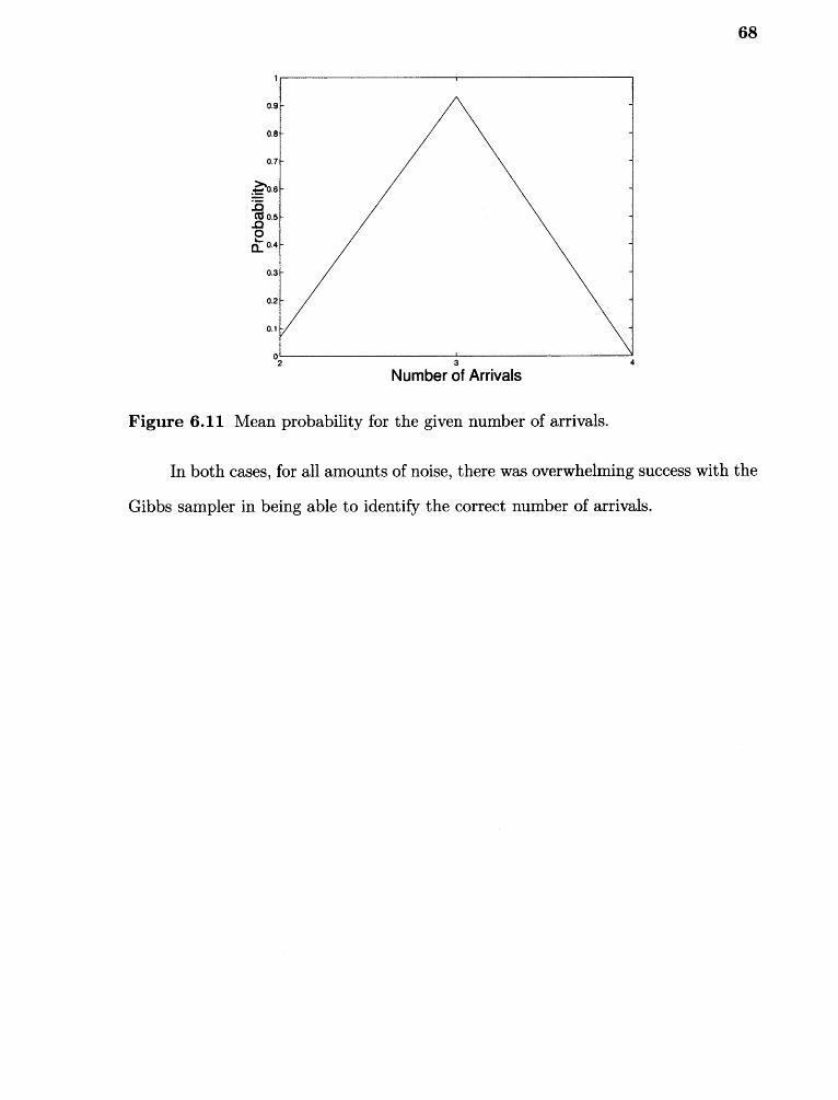
0.9
0.8
0.7
>•■0.6
23CC 0.5
0Ft 0.4
68
3
4
Number of Arrivals
Figure 6.11 Mean probability for the given number of arrivals.
In both cases, for all amounts of noise, there was overwhelming success with the
Gibbs sampler in being able to identify the correct number of arrivals.
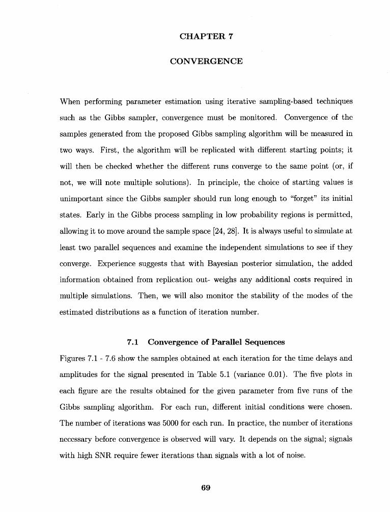
CHAPTER 7
CONVERGENCE
When performing parameter estimation using iterative sampling-based techniques
such as the Gibbs sampler, convergence must be monitored. Convergence of the
samples generated from the proposed Gibbs sampling algorithm will be measured in
two ways. First, the algorithm will be replicated with different starting points; it
will then be checked whether the different runs converge to the same point (or, if
not, we will note multiple solutions). In principle, the choice of starting values is
unimportant since the Gibbs sampler should run long enough to "forget" its initial
states. Early in the Gibbs process sampling in low probability regions is permitted,
allowing it to move around the sample space [24, 28]. It is always useful to simulate at
least two parallel sequences and examine the independent simulations to see if they
converge. Experience suggests that with Bayesian posterior simulation, the added
information obtained from replication out- weighs any additional costs required in
multiple simulations. Then, we will also monitor the stability of the modes of the
estimated distributions as a function of iteration number.
7.1 Convergence of Parallel Sequences
Figures 7.1 - 7.6 show the samples obtained at each iteration for the time delays and
amplitudes for the signal presented in Table 5.1 (variance 0.01). The five plots in
each figure are the results obtained for the given parameter from five runs of the
Gibbs sampling algorithm. For each run, different initial conditions were chosen.
The number of iterations was 5000 for each run. In practice, the number of iterations
necessary before convergence is observed will vary. It depends on the signal; signals
with high SNR require fewer iterations than signals with a lot of noise.
69
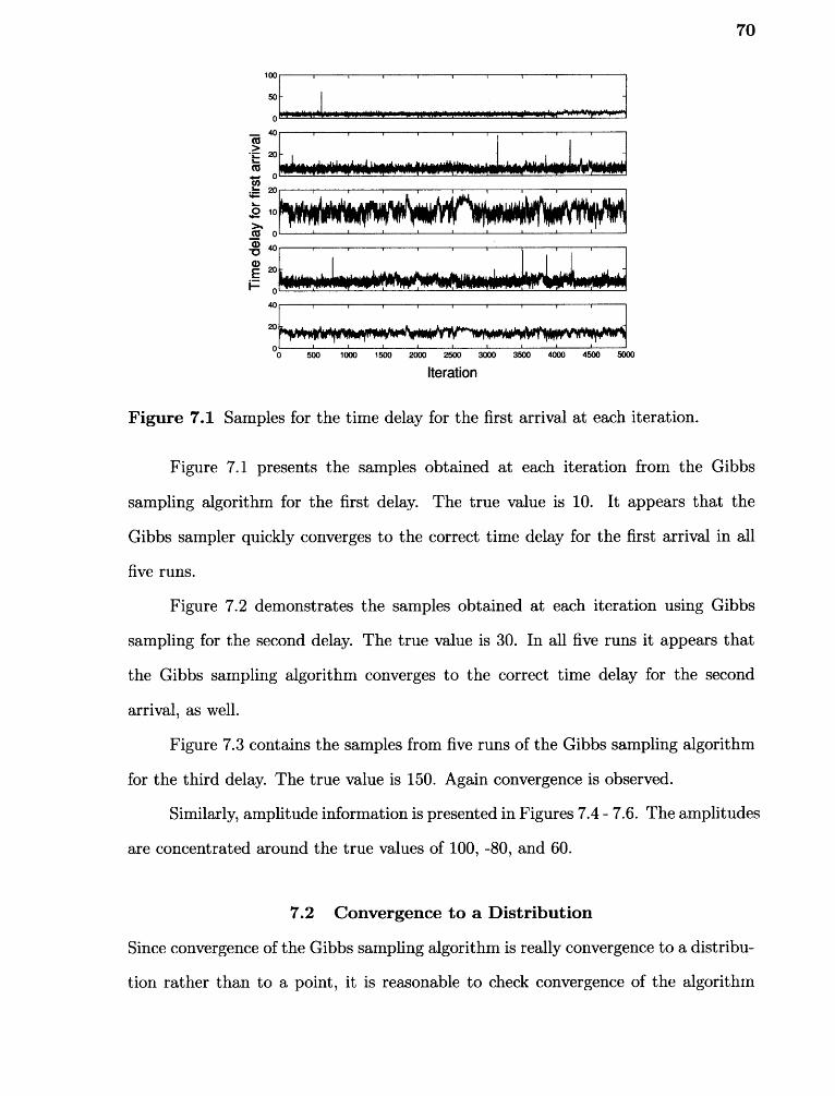
ooh500 1000 1500 3500 4000 7500 50002900 2500 3000
70
20o
-
1 i t
40
20
i 20o
F.3 020
O;410
co
•
0▪70
a)
I-
70
I I I I I I I I
Iteration
Figure 7.1 Samples for the time delay for the first arrival at each iteration.
Figure 7.1 presents the samples obtained at each iteration from the Gibbs
sampling algorithm for the first delay. The true value is 10. It appears that the
Gibbs sampler quickly converges to the correct time delay for the first arrival in all
five runs.
Figure 7.2 demonstrates the samples obtained at each iteration using Gibbs
sampling for the second delay. The true value is 30. In all five runs it appears that
the Gibbs sampling algorithm converges to the correct time delay for the second
arrival, as well.
Figure 7.3 contains the samples from five runs of the Gibbs sampling algorithm
for the third delay. The true value is 150. Again convergence is observed.
Similarly, amplitude information is presented in Figures 7.4 - 7.6. The amplitudes
are concentrated around the true values of 100, -80, and 60.
7.2 Convergence to a Distribution
Since convergence of the Gibbs sampling algorithm is really convergence to a distribu-
tion rather than to a point, it is reasonable to check convergence of the algorithm
100
500
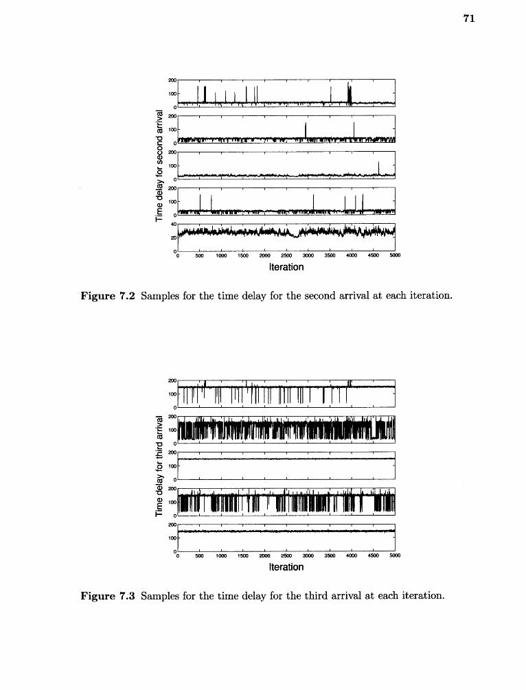
-6 290
as 100
C00 200a)cif)
1000
>• 0fats290
O00
Bo
20
2900 2500 3000
Iteration
ooh500 1000 1500 3500 4000 4500 5000
Figure 7.2 Samples for the time delay for the second arrival at each iteration.
100
290
*E 100cribp 0
290
O 100
c 0
290
100
71
2000 2500 3000
Iteration
290
100
00
500
1000
1500 3500
4000
4500
5000
Figure 7.3 Samples for the time delay for the third arrival at each iteration.
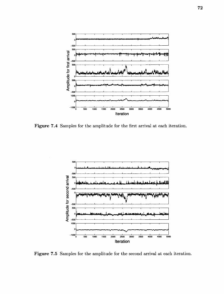
Iteration
Figure 7.4 Samples for the amplitude for the first arrival at each iteration.
500
0
-500
TC 500>
id"Ac -500
O 0C.)a)co
8-500
a)-A 500Z
-aE
< -500
2900 2500 3000
3500
7000
4500
5000
Iteration
Figure 7.5 Samples for the amplitude for the second arrival at each iteration.
72
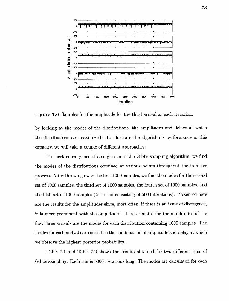
73
- 290
500
0
-500
• 290
a) -290
500
-EL 0
-500
290
0
- 2900
500
1000
1500 2000 2500 3000
3500
7000
4500
5000
Iteration
Figure 7.6 Samples for the amplitude for the third arrival at each iteration.
by looking at the modes of the distributions, the amplitudes and delays at which
the distributions are maximized. To illustrate the algorithm's performance in this
capacity, we will take a couple of different approaches.
To check convergence of a single run of the Gibbs sampling algorithm, we find
the modes of the distributions obtained at various points throughout the iterative
process. After throwing away the first 1000 samples, we find the modes for the second
set of 1000 samples, the third set of 1000 samples, the fourth set of 1000 samples, and
the fifth set of 1000 samples (for a run consisting of 5000 iterations). Presented here
are the results for the amplitudes since, most often, if there is an issue of divergence,
it is more prominent with the amplitudes. The estimates for the amplitudes of the
first three arrivals are the modes for each distribution containing 1000 samples. The
modes for each arrival correspond to the combination of amplitude and delay at which
we observe the highest posterior probability.
Table 7.1 and Table 7.2 shows the results obtained for two different runs of
Gibbs sampling. Each run is 5000 iterations long. The modes are calculated for each
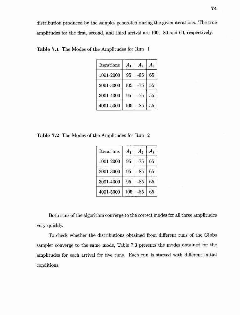
74
distribution produced by the samples generated during the given iterations. The true
amplitudes for the first, second, and third arrival are 100, -80 and 60, respectively.
Table 7.1 The Modes of the Amplitudes for Run 1
Iterations A l A2 A3
1001-2000 95 -85 65
1001-3000 105 -75 55
3001-4000 95 -75 55
4001-5000 105 -85 55
Table 7.2 The Modes of the Amplitudes for Run 2
Iterations A l Ay A3
1001-2000 95 -75 65
1001-3000 95 -85 65
3001-4000 95 -85 65
4001-5000 105 -85 65
Both runs of the algorithm converge to the correct modes for all three amplitudes
very quickly.
To check whether the distributions obtained from different runs of the Gibbs
sampler converge to the same mode, Table 7.3 presents the modes obtained for the
amplitudes for each arrival for five runs. Each run is started with different initial
conditions.
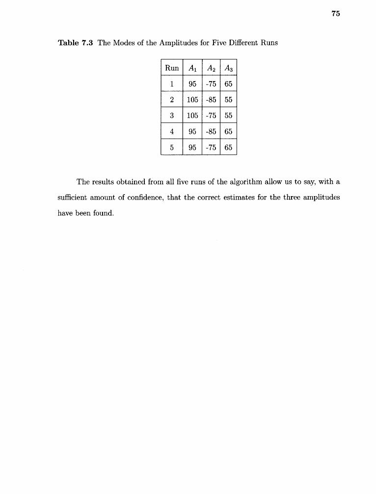
75
Table 7.3 The Modes of the Amplitudes for Five Different Runs
Run A l Ay A3
1 95 -75 65
2 105 -85 55
3 105 -75 55
4 95 -85 65
5 95 -75 65
The results obtained from all five runs of the algorithm allow us to say, with a
sufficient amount of confidence, that the correct estimates for the three amplitudes
have been found.
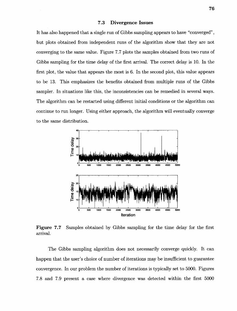
76
7.3 Divergence Issues
It has also happened that a single run of Gibbs sampling appears to have "converged" ,
but plots obtained from independent runs of the algorithm show that they are not
converging to the same value. Figure 7.7 plots the samples obtained from two runs of
Gibbs sampling for the time delay of the first arrival. The correct delay is 10. In the
first plot, the value that appears the most is 6. In the second plot, this value appears
to be 13. This emphasizes the benefits obtained from multiple runs of the Gibbs
sampler. In situations like this, the inconsistencies can be remedied in several ways.
The algorithm can be restarted using different initial conditions or the algorithm can
continue to run longer. Using either approach, the algorithm will eventually converge
to the same distribution.
Iteration
Figure 7.7 Samples obtained by Gibbs sampling for the time delay for the firstarrival.
The Gibbs sampling algorithm does not necessarily converge quickly. It can
happen that the user's choice of number of iterations may be insufficient to guarantee
convergence. In our problem the number of iterations is typically set to 5000. Figures
7.8 and 7.9 present a case where divergence was detected within the first 5000
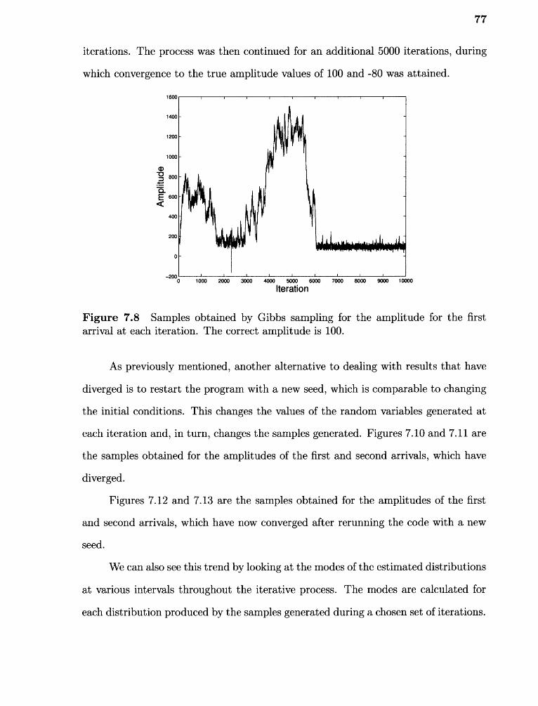
■1 000
-20003000
12000
77
iterations. The process was then continued for an additional 5000 iterations, during
which convergence to the true amplitude values of 100 and -80 was attained.
1600
1400 -
1200 -
1000
a)= 800:toa.E 600<
700
200
7000 5000 6000
Iteration. , ■
7000 8000 9000 1 0000
Figure 7.8 Samples obtained by Gibbs sampling for the amplitude for the firstarrival at each iteration. The correct amplitude is 100.
As previously mentioned, another alternative to dealing with results that have
diverged is to restart the program with a new seed, which is comparable to changing
the initial conditions. This changes the values of the random variables generated at
each iteration and, in turn, changes the samples generated. Figures 7.10 and 7.11 are
the samples obtained for the amplitudes of the first and second arrivals, which have
diverged.
Figures 7.12 and 7.13 are the samples obtained for the amplitudes of the first
and second arrivals, which have now converged after rerunning the code with a new
seed.
We can also see this trend by looking at the modes of the estimated distributions
at various intervals throughout the iterative process. The modes are calculated for
each distribution produced by the samples generated during a chosen set of iterations.
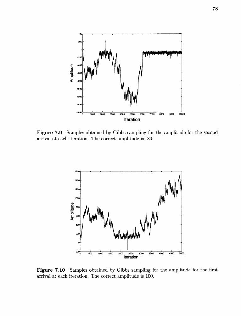
290
—200
Q)
=—600 —.Q
E< —800 -
—1000 -
—1200 —
—1400 —
—16000
1 a 1 a 1 t 1 1 1
1 000 2900 3000 7000 5000 6000 7000 8000 9000 10000
50001000
1500
1600
1400
1290
1000
a)73= 800
CIE 600< to
2900 2500 3000
Iterationt 1 t
3500 7000 4500
700
78
Iteration
Figure 7.9 Samples obtained by Gibbs sampling for the amplitude for the secondarrival at each iteration. The correct amplitude is -80.
Figure 7.10 Samples obtained by Gibbs sampling for the amplitude for the firstarrival at each iteration. The correct amplitude is 100.
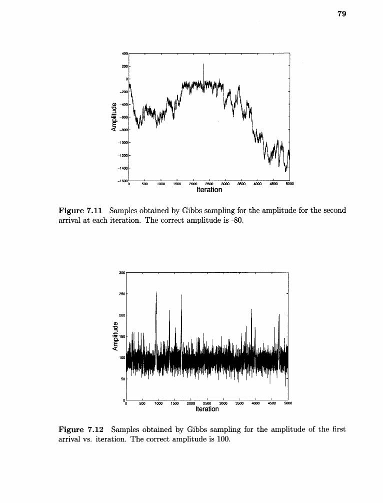
79
Iteration
Figure 7.11 Samples obtained by Gibbs sampling for the amplitude for the secondarrival at each iteration. The correct amplitude is -80.
300
250
200
a)13=:11150
E<100
50
300 500 1000 1500 2000 2500 3000
Iteration3500 7000 4500 5000
Figure 7.12 Samples obtained by Gibbs sampling for the amplitude of the firstarrival vs. iteration. The correct amplitude is 100.
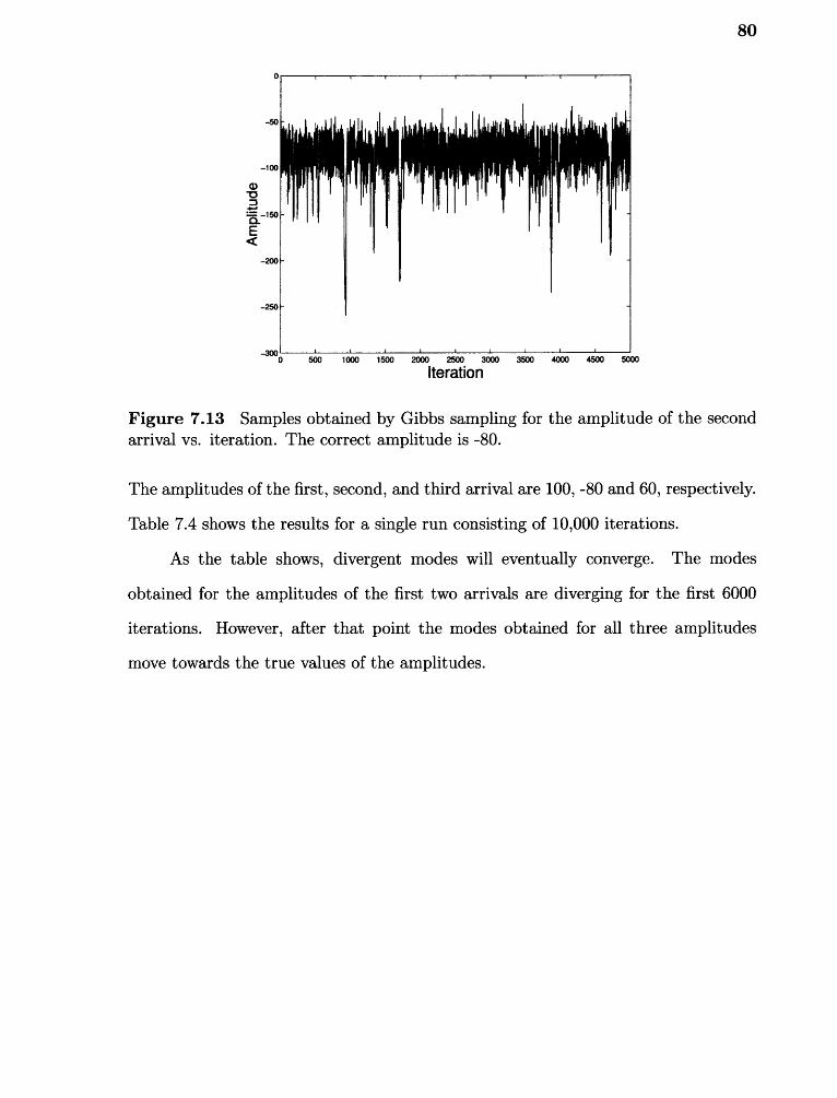
80
0
-50
-100
-azLa.-150
E
-
2000
-250
- 3000 7000 4500 500035001000500 1500 2000 2500 3000
Iteration
Figure 7.13 Samples obtained by Gibbs sampling for the amplitude of the secondarrival vs. iteration. The correct amplitude is -80.
The amplitudes of the first, second, and third arrival are 100, -80 and 60, respectively.
Table 7.4 shows the results for a single run consisting of 10,000 iterations.
As the table shows, divergent modes will eventually converge. The modes
obtained for the amplitudes of the first two arrivals are diverging for the first 6000
iterations. However, after that point the modes obtained for all three amplitudes
move towards the true values of the amplitudes.
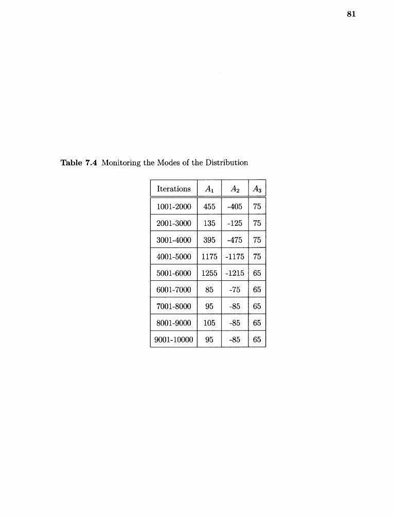
Table 7.4 Monitoring the Modes of the Distribution
Iterations A l A2 A3
1001-2000 455 -405 75
1001-3000 135 -125 75
3001-4000 395 -475 75
4001-5000 1175 -1175 75
5001-6000 1255 -1215 65
6001-7000 85 -75 65
7001-8000 95 -85 65
8001-9000 105 -85 65
9001-10000 95 -85 65
81
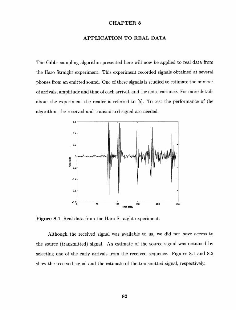
CHAPTER 8
APPLICATION TO REAL DATA
The Gibbs sampling algorithm presented here will now be applied to real data from
the Haro Straight experiment. This experiment recorded signals obtained at several
phones from an emitted sound. One of these signals is studied to estimate the number
of arrivals, amplitude and time of each arrival, and the noise variance. For more details
about the experiment the reader is referred to [5]. To test the performance of the
algorithm, the received and transmitted signal are needed.
50 100 150
200Time delay
Figure 8.1 Real data from the Haro Straight experiment.
Although the received signal was available to us, we did not have access to
the source (transmitted) signal. An estimate of the source signal was obtained by
selecting one of the early arrivals from the received sequence. Figures 8.1 and 8.2
show the received signal and the estimate of the transmitted signal, respectively.
82
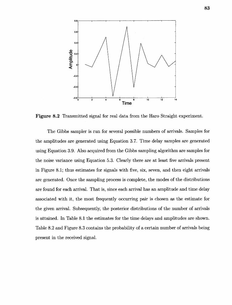
83
Figure 8.2 Transmitted signal for real data from the Haro Straight experiment.
The Gibbs sampler is run for several possible numbers of arrivals. Samples for
the amplitudes are generated using Equation 3.7. Time delay samples are generated
using Equation 3.9. Also acquired from the Gibbs sampling algorithm are samples for
the noise variance using Equation 5.3. Clearly there are at least five arrivals present
in Figure 8.1; thus estimates for signals with five, six, seven, and then eight arrivals
are generated. Once the sampling process is complete, the modes of the distributions
are found for each arrival. That is, since each arrival has an amplitude and time delay
associated with it, the most frequently occurring pair is chosen as the estimate for
the given arrival. Subsequently, the posterior distributions of the number of arrivals
is attained. In Table 8.1 the estimates for the time delays and amplitudes are shown.
Table 8.2 and Figure 8.3 contains the probability of a certain number of arrivals being
present in the received signal.
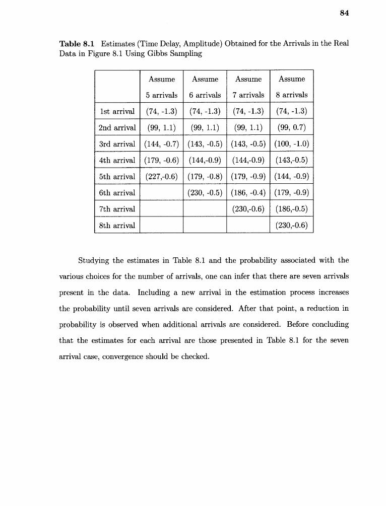
84
Table 8.1 Estimates (Time Delay, Amplitude) Obtained for the Arrivals in the RealData in Figure 8.1 Using Gibbs Sampling
Assume
5 arrivals
Assume
6 arrivals
Assume
7 arrivals
Assume
8 arrivals
1st arrival (74, -1.3) (74, -1.3) (74, -1.3) (74, -1.3)
2nd arrival (99, 1.1) (99, 1.1) (99, 1.1) (99,0.7)
3rd arrival (144, -0.7) (143, -0.5) (143, -0.5) (100,-1.0)
4th arrival (179, -0.6) (144,-0.9) (144,-0.9) (143,-0.5)
5th arrival (227,-0.6) (179, -0.8) (179, -0.9) (144, -0.9)
6th arrival (230, -0.5) (186, -0.4) (179, -0.9)
7th arrival (230,-0.6) (186,-0.5)
8th arrival (230,-0.6)
Studying the estimates in Table 8.1 and the probability associated with the
various choices for the number of arrivals, one can infer that there are seven arrivals
present in the data. Including a new arrival in the estimation process increases
the probability until seven arrivals are considered. After that point, a reduction in
probability is observed when additional arrivals are considered. Before concluding
that the estimates for each arrival are those presented in Table 8.1 for the seven
arrival case, convergence should be checked.
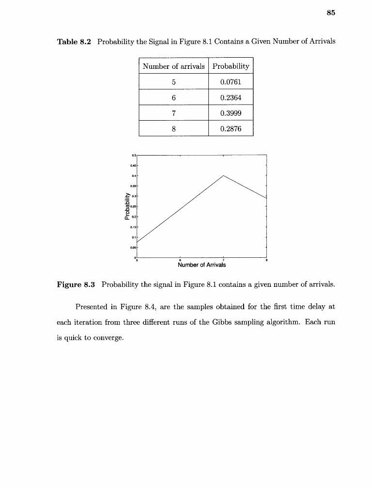
85
Table 8.2 Probability the Signal in Figure 8.1 Contains a Given Number of Arrivals
Number of arrivals Probability
5 0.0761
6 0.2364
7 0.3999
8 0.2876
6 7
Number of Arrivals
Figure 8.3 Probability the signal in Figure 8.1 contains a given number of arrivals.
Presented in Figure 8.4, are the samples obtained for the first time delay at
each iteration from three different runs of the Gibbs sampling algorithm. Each run
is quick to converge.
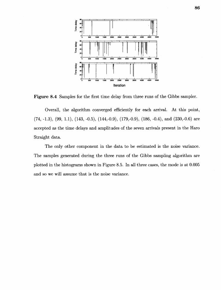
86
-AE
566 1666 1566 2666 2566 3066 3506 2606 2566
1 I
■566 1666 1566 2566 3066 566 2666 4566
506 1666 1566 2666 2566 3066 3506 2066 4566
Iteration
Figure 8.4 Samples for the first time delay from three runs of the Gibbs sampler.
Overall, the algorithm converged efficiently for each arrival. At this point,
(74, -1.3), (99, 1.1), (143, -0.5), (144,-0.9), (179,-0.9), (186, -0.4), and (230,-0.6) are
accepted as the time delays and amplitudes of the seven arrivals present in the Haro
Straight data.
The only other component in the data to be estimated is the noise variance.
The samples generated during the three runs of the Gibbs sampling algorithm are
plotted in the histograms shown in Figure 8.5. In all three cases, the mode is at 0.005
and so we will assume that is the noise variance.
so
so20
20
5005666
5666
40
86
566
20
I 1 A-,5666
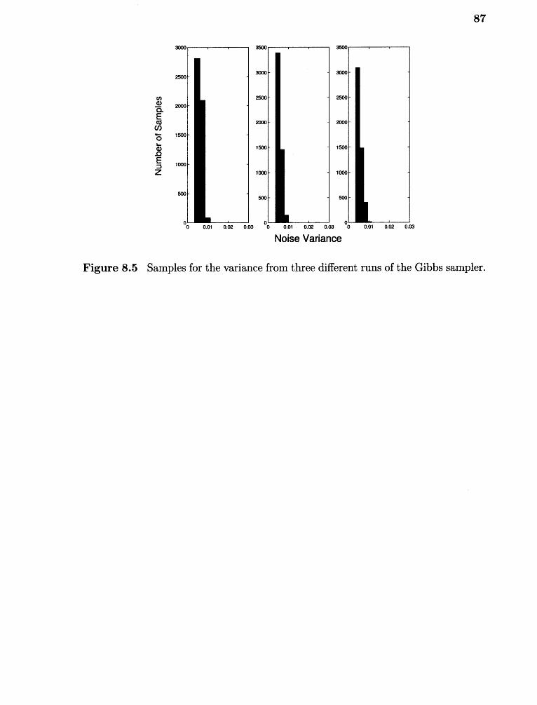
3500
3000
2500
2000
1500
1000
500
ace0.05 0.03
3500
3000
2500
2000
1500
1000
500
o 0 0 0.05 0.02 0.03 0
Noise Variance
87
Figure 8.5 Samples for the variance from three different runs of the Gibbs sampler.
CHAPTER 9
CONCLUSIONS
In this work, an approach for the calculation of maximum a posteriori estimates
for time delays, amplitudes, noise, and number of arrivals using a Gibbs sampling
optimization method is developed. It has been shown that the approach is efficient
to implement and can compute maximum a posteriori estimates rapidly in cases of
several multi-paths, when the analytical maximum a posteriori approach is computa-
tionally not feasible.
The proposed Gibbs sampler was initially applied to synthetic data. Several
cases were examined, testing the performance relative to the signal-to-noise ratio,
number of multi-path arrivals, and time between the distinct arrivals. The results
presented here have exhibited superiority to other optimization methods. The pro-
posed method is faster than simulating annealing. It does not dependent on initial
conditions like EM, and does not present any difficulties with closely spaced arrivals
encountered with MF. In addition to efficiency and accuracy in the estimates, the
Gibbs sampling method has the additional advantage of computing an estimate of
the entire joint probability distribution of the unknown parameters, in contrast to
most other methods that result only on point estimates, giving a more informative
picture of the problem at hand.
The algorithm was also tested for convergence. This issue was approached in two
different ways: First by checking parallel runs of the algorithm and then by examining
the modes of the distribution. Convergence was typically attained within a relatively
small number of iterations. On a few occasions, additional runs or iterations were
necessary for the posterior distributions to stabilize.
88
89
The method was also applied to the Haro Straight data. Given a time series,
the number of arrivals was recovered. Once this number was decided and the samples
were checked for convergence, estimates were obtained for the time delays, amplitudes,
and noise variance.
The work presented here can be further extended, treating the Gibbs sampler
as the first step in a two step process. First, generate samples to determine values
for the time delays, amplitudes, noise variance, and number of multi-paths. Once
estimates are obtained for the parameters associated with the received signal, they
can then be used to quickly find estimates for the parameters associated with the
problem of interest, such as source and receiver location, sound speed profile, bottom
properties, etc, in shallow water propagation.
BIBLIOGRAPHY
[1] A. Nehorai and S. Li, "An asymptotic maximum likelihood estimator for sourceparameters in a multipath environment," IEEE, pp. 2630-2633, 1988.
[2] J. lanniello, "High-resolution multipath time delay estimation for broad-band randomsignals," IEEE Transactions on Acoustics, Speech, and Signal Processing, vol. 36,pp. 320-327, 1988.
[3] W. Hahn and S. Tretter, "Optimum processing for delay-vector estimation in passivesignal arrays," IEEE Transactions on Information Theory, vol. 19, pp. 608-614,1973
[4] S. Dosso, M. Fallat, B. Sotirin, and J. Newton, "Array element localizationfor horizontal arrays via occam's inversion," J. Acoust. Soc. Am., vol. 104,pp. 846-859, 1998.
[5] X. Ma, Efficient Inversion Methods In Underwater Acoustics. PhD thesis, New JerseyInstitute of Technology, 1001.
[6] F. Jensen, W. Kuperman, M. Porter, and H. Schmidt, Computational OceanAcoustics. New York: American Institute of Physics, 1994.
[7] M. B. Porter, "The KRAKEN normal mode program," SACLANT Undersea ResearchCentre Memorandum (SM-245) and Naval Research Laboratory Mem. Rep. 6920,1991
[8] A. Baggeroer, W. Kuperman, and P. N. Michalevsky, "An overview of matched fieldprocessing in ocean acoustics," IEEE Journal of Oceanic Engineering, vol. 18,pp. 401-424, 1993.
[9] A. Tolstoy, Matched Field Processing for Underwater Acoustics. Singapore: WorldScientific, 1993.
[10] M. D. Collins and W. Kuperman, "Focalization: Environmental focusing and sourcelocalization," J. Acoust. Soc. Am., pp. 1410-1422, 1991.
[11] J. F. Smith and S. Finette, "Simulated annealing as a method of deconvolution foracoustic transients measured on a vertical array," J. Acoust. Soc. Am., pp. 2315-2325, 1993.
[12] M. Feder and E. Weinstein, "Parameter estimation of superimposed signals using theEM algorithm," IEEE Transactions on Acoustics, Speech, and Signal Processing,vol. 36, pp. 477-489, 1988.
90
91
[13] A. Blackowiak and S. Rajan, "Multi-path arrival estimates using simulated annealing;application to crosshole tomography experiment," IEEE Journal of OceanicEngineering, pp. 157-165,1995.
[14] L. Jaschke and N. Chapman, "Matched field inversion of broadband data using thefreeze bath method." Submitted to J. Acoust. Soc. Am., 1998.
[15] P. Pignot and R. Chapman, "Tomographic inversion for geoacoustic properties in arange dependent shallow water evvironment." Submitted to J. Acoust. Soc. Am.,1998.
[16] J. Ehrenberg, T. Ewart, and R. Morris, "Signal-processing techniques for resolvingindividual pulses in a multipath signal," J. Acoust. Soc. Am., pp. 1861-1865,1978.
[17] R. J. Vaccaro and R. L. Field, "Transient signal extraction in a multipathenvironment," IEEE, pp. 115-120,1990.
[18] T. G. Manickam, R. J. Vaccaro, and D. W. Tufts, "A least-squares algorithmfor multipath time-delay estimation," IEEE Transactions on Signal Processing,vol. 42, pp. 3229-3233,1994.
[191] L. Jaschke, "Geophysical inversion by the freeze bath method with an applicationto geoacoustic ocean bottom parameter estimation," Master's thesis, School ofEarth and Ocean Science, 1997.
[20] G. J. McLachlan and T. Krishnan,The EM Algorithm and Extensions.New York,NY: John Wiley Sons, Inc., 1997.
[21] I. Ziskind and M. Wax, "Maximum likelihood localization of multiple sources byalternating projection," IEEE Transactions on Acoustics, Speech, and SignalProcessing, vol. 36, pp. 1553-1560,1988.
[22] M. Feder and E. Weinstein, "An EM algorithm for multisensor tdoa/dd estimationin a multipath propagation environment," IEEE, pp. 3117-3120,1996.
[23] M. Sen, P. L. Stoffa, and H. Schmidt, Global Optimization Methods in GeophysicalInversion. Elsevier, 1995.
[24] W. R. Gilks, S. Richardson, and D. J. Spiegelhalter, Markov Chain Monte Carlo inPractice. Chapman and Hall/CRC, 1996.
[25] A. E. Gelfand, A. F. M. Smith, and T.-M. Lee, "Bayesian analysis of constrainedparameter and truncated data problems using gibbs sampling," Journal of theAmerical Statistical Association, vol. 87, pp. 523-532,1992.
[26] S. Geman and D. Geman, "Stochastic relaxation, gibbs distributions, and the bayesianrestoration of images," IEEE Transactions on Pattern Analysis and MachineIntelligence, pp. 721-741,1984.
92
[27] A. Gelfand, S. Hills, A. Racine-Poon, and A. Smith, "Illustration of bayesian inferencein normal data models using gibbs sampling," Journal of the American StatisticalAssociation, vol. 85, pp. 972-985, 1990.
[28] G. Casella and E. I. George, "Explaining the gibbs sampler," The AmericanStatistician, vol. 46, pp. 167-174, 1992.
[29] A. Whalen, Detection of Signals in Noise. California: Academic Press, Inc., 1971.
[30] S. M. Ross, Introduction To Probability Models. Academy Press, 1997.
[31] R. Hogg and E. Tanis, Probability and Statistical Inference. Macmillan, 1993.
[32] Z.-H. Michalopoulou, X. Ma, M. Picarelli, and U. Ghosh-Dastidar, "Fast matchingmethods for inversion with underwater sound," in Proceedings of Ocean 2000,(Rhode Island), 1000.
[33] A. Tolstoy, N. R. Chapman, and G. Brooke, "Workshop '97: Benchmarking forgeoacoustic inversion in shallow water," Journal of Computational Acoustics,vol. 6, pp. 1-28, 1998.
[34] G. Box and G. Tiao, Bayesian Inference in Statistical Analysis. Philippines: Addison-Wesley Publishing Company, Inc., 1973.
[35] R. Vaccaro, C. Ramalingam, and D. Tufts, "Least-squares time-delay estimation fortransient signals in a multipath environment," J. Acoust. Soc. Am., vol. 92,pp. 210-218, 1992.
[36] M. Wax and T. Kailath, "Detection of signals by information theoretic criteria," IEEETransactions on Acoustics, Speech, and Signal Processing, vol. 33, pp. 387-392,1985.