COMP5348

Lecture 6:

Predicting Performance

Adapted with permission from presentations by Alan Fekete

Outline

Approaches to Performance Prediction Operational Laws Performance bounds for closed systems M/M/1 systems

Extrapolation

Measure the performance for some values of vital parameters Eg measure response time with 10, 20, 30 clients

Fit a curve through the measured data Use the curve to predict performance for other

values of parameters

Big problem: performance can change radically when system reaches capacity Interpolation works well, but not extrapolation

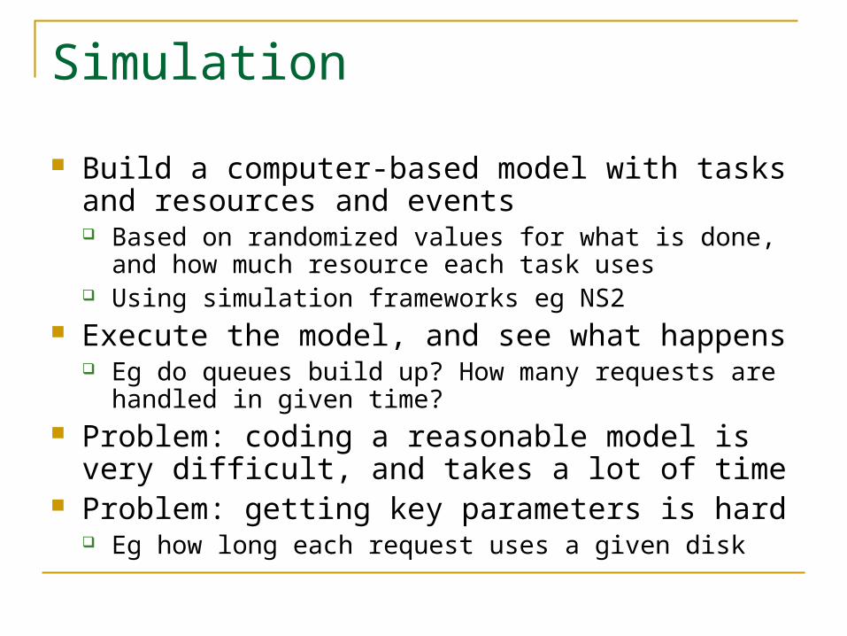
Simulation

Build a computer-based model with tasks and resources and events Based on randomized values for what is done, and how

much resource each task uses Using simulation frameworks eg NS2

Execute the model, and see what happens Eg do queues build up? How many requests are handled in

given time? Problem: coding a reasonable model is very difficult,

and takes a lot of time Problem: getting key parameters is hard

Eg how long each request uses a given disk

Analytical (Queuing) Models Build a mathematical model, with resources and

queues and probabilities for state transitions Solve for the steady state behaviour

Either exact solution (as a function) Or approximate solution of the relevant equations by

iteration Not as precise as simulation, but usually far easier Some simple results can be done back-of-an-

envelope, without depending on precise knowledge of the distribution of random values

Basic probability (discrete cases) P(A): the fraction of occurrences of event A among all possible

cases Eg cases are all possible ways to toss 20 coins One case is HTHHTHTHTTHTTTTHHHTH A case is a simple event P(HTHHTHTHTTHTTTTHHHTH)=1/220

One event is “A1: fourth toss is heads”; P(A1)=0.5 Another event is “A2: First head is at toss 4”; P(A2)=0.0625

P(A) must be between 0 and 1 (inclusive) What does P(A)=0 mean?

P(not A) = 1 - P(A) P(A and B) = P(A)*P(B)

If A independent of B (they are not correlated) P(A or B) = P(A)+P(B)-P(A and B)

Approximately P(A)+P(B) if A independent of B, and both are rare

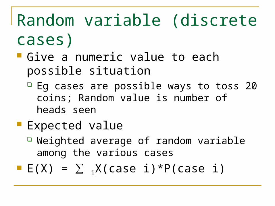
Random variable (discrete cases) Give a numeric value to each possible

situation Eg cases are possible ways to toss 20 coins;

Random value is number of heads seen Expected value

Weighted average of random variable among the various cases

E(X) = ∑ iX(case i)*P(case i)

Uniform distribution (discrete cases) Integer valued random variable All values are equally likely, within the range

allowed

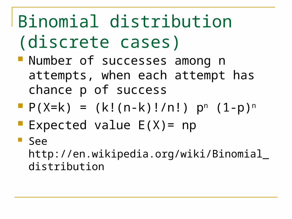
Binomial distribution (discrete cases) Number of successes among n attempts,

when each attempt has chance p of success P(X=k) = (k!(n-k)!/n!) pn (1-p)n

Expected value E(X)= np See http://en.wikipedia.org/wiki/Binomial_distribution

Continuous cases

Where there are infintely many possible situations Eg each situation is one execution of a system

Assign probabilities to events An event is a subset of situations Eg event is”no processor crashed during the execution” Or “the 5th request was processed at node 17” Events can overlap with one another

Random variable is a value associated with each situation Eg “the number of requests processed during the

execution” Probability density function

Uniform distribution

Discrete cases: All values are equally likely, with a finite set of allowed values Continuous cases: Any range has probability

proportional to the length of the range (as long as range is within the set of allowed values)

Eg “all file lengths are equally likely, from 0 bytes to 1 Mbyte”

Easy to work with mathematically, but may not be an accurate approximation to reality!

Normal distribution

Two parameters and Pdf(x) = ( √( 2 ))-1 exp( -(x- )2/2 ) Distribution is symmetric around X=

Expected value is is a measure of the spread

Many real situations are closely approximated as normal distributions Combined impact of many independent variations

See http://en.wikipedia.org/wiki/Normal_distribution

Exponential distribution

One parameter Pdf(x) = exp(- x)

Expected value = 1/ Memoryless distribution

Time between events, if the past has no impact on the future

See http://en.wikipedia.org/wiki/Exponential_distribution

Poisson distribution

Number of occurrences of an event with exponential distribution on inter-event gaps A good approximation to binomial distribution

when np= , and n is big and p is small The probability of having value k is

Prob(k) = (k exp(-))/k! Expected value =

See http://en.wikipedia.org/wiki/Poisson_distribution

Outline

Approaches to Performance Prediction Operational Laws Performance bounds for closed systems M/M/1 systems

The main independent parameter For a closed system

N: the number of clients that submit jobs Also, the number of jobs

that are either in the system, or “thinking” at the client

Z: think time, between when a job is completed and when the same client submits another job

For an open system : the arrival rate of jobs

per second

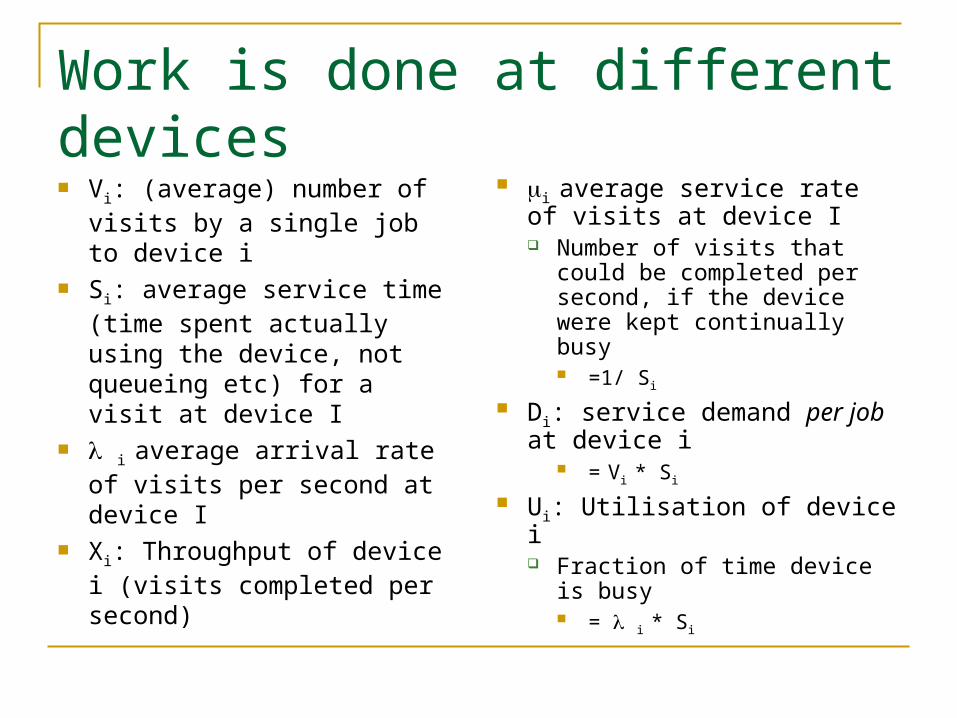
Work is done at different devices Vi: (average) number of

visits by a single job to device i

Si: average service time (time spent actually using the device, not queueing etc) for a visit at device I

i average arrival rate of visits per second at device I

Xi: Throughput of device i (visits completed per second)

i average service rate of visits at device I Number of visits that could

be completed per second, if the device were kept continually busy =1/ Si

Di: service demand per job at device i

= Vi * Si

Ui: Utilisation of device i Fraction of time device is

busy = i * Si

The main performance measures Throughput X: the (average)

number of jobs completed per second

Response time R: the (average) time

from submitting a job till it is completed

Little’s Law

N = T Applies to any system in steady state

N is number of jobs in the “system” T is the average time spent in the “system” is the average rate of arrival (or departure) from the system

This law can be applied to any part of the system It doesn’t depend on knowing the shape of the distribution

of parameters It can be applied to a larger whole with a closed

computer-system plus the clients N = X*(R+Z), that is, R = N/X - Z

This is called “interactive response time law”

Relating a device to the whole system Forced Flow Law

Xi = Vi * X

Service Demand Law (“Bottleneck Law”) Ui = Di * X

Outline

Approaches to Performance Prediction Operational Laws Performance bounds for closed systems M/M/1 systems

Performance bounds

Let Dmax be the largest among the Di

The device i where the max occurs is called the “bottleneck” for the system

X <= 1/ Dmax

Because Ui must be at most 1.

So R >= N* Dmax - Z X and R are close to the bounds, when load

is high

Performance bounds

Let D be the sum of all the Di

R >= D Because the total time to deal with a job includes

the time at each device, plus also queuing time So X <= N/ (D + Z) X and R are close to the bounds, when load

is low

Effect of the bounds

N

X

N

R

1/Dmax

Queues start to build upbadly, as bottleneck is saturated

Low load bound

Low load bound

High load bound

High load bound

System design

The bottleneck is the device i with largest Di

The only way to get better throughput than 1/ Dmax is to change the system design to change Dmax Move some tasks away from the bottleneck device

Add some new devices to take some of the load Or re-arrange processing so some visits go to other existing

devices instead Or, change the nature of the device so each request needs

less service time Eg change for a faster disk

After the system is redesigned, there will still be a bottleneck! Perhaps on a different device

Outline

Approaches to Performance Prediction Operational Laws Performance bounds for closed systems M/M/1 systems

M/M/1

Assume jobs arrive by Poisson process Inter-arrival time gap has exponential distribution Average number of arrivals per second is

Assume the service demand is also exponential distribution Average number of services possible per second

is The essential parameter is load , defined by

/

M/M/1 Queuing Theory

Average number of jobs in (queue or being served) is N = /(1- )

Average number of jobs in queue is Nwait Nwait = 2/(1- )

Average time in system (waiting or being served) is T = 1/ (1- )

Average waiting time in queue is Twait= / (1- )

Impact of queues

If is close to , then the queue builds up to be long And each job is delayed a long time Note contrast with situation of exactly periodic arrival of

jobs, and exactly equal service times, where there is never a queue as long as is below

We aim to keep load at the bottleneck resource to be below 0.8, say Thus we do not let any resource get saturated

Heavy tailed distributions In general, distributions which are spread

more from the average have longer queues and worse response times

This is especially serious for distributions like power-laws, where the few extremely big jobs can clog the system giving bad response time for every job

Further reading

D. Menasce, V. Almeida, L. Dowdy “Performance by Design”, pub by Prentice-Hall, 2004