Copyright © Cengage Learning. All rights reserved.

4 Applications of Differentiation

Copyright © Cengage Learning. All rights reserved.

4.2 The Mean Value Theorem

3

The Mean Value Theorem

We will see that many of the results depend on one central fact, which is called the Mean Value Theorem. But to arrive at the Mean Value Theorem we first need the following result.

Before giving the proof let’s take a look at the graphs of some typical functions that satisfy the three hypotheses.

4

The Mean Value Theorem

Figure 1 shows the graphs of four such functions.

Figure 1

(c)

(b)

(d)

(a)

5

The Mean Value Theorem

In each case it appears that there is at least one point (c, f (c)) on the graph where the tangent is horizontal and therefore f (c) = 0.

Thus Rolle’s Theorem is plausible.

6

Example 2

Prove that the equation x3 + x – 1 = 0 has exactly one real root.

Solution:First we use the Intermediate Value Theorem to show that a root exists. Let f (x) = x3 + x – 1. Then f (0) = –1 < 0 and f (1) = 1 > 0.

Since f is a polynomial, it is continuous, so the Intermediate Value Theorem states that there is a number c between 0 and 1 such that f (c) = 0.

Thus the given equation has a root.

7

Example 2 – Solution

To show that the equation has no other real root, we use Rolle’s Theorem and argue by contradiction.

Suppose that it had two roots a and b. Then f (a) = 0 = f (b) and, since f is a polynomial, it is differentiable on (a, b) and continuous on [a, b].

Thus, by Rolle’s Theorem, there is a number c between a and b such that f (c) = 0.

cont’d

8

Example 2 – Solution

But

f (x) = 3x2 + 1 1 for all x

(since x2 0) so f (x) can never be 0. This gives a contradiction.

Therefore the equation can’t have two real roots.

cont’d

9

The Mean Value Theorem

Our main use of Rolle’s Theorem is in proving the following important theorem, which was first stated by another French mathematician, Joseph-Louis Lagrange.

10

The Mean Value Theorem

Before proving this theorem, we can see that it is reasonable by interpreting it geometrically. Figures 3 and 4 show the points A (a, f (a)) and B (b, f (b)) on the graphs oftwo differentiable functions.

Figure 3 Figure 4

11

The Mean Value Theorem

The slope of the secant line AB is

which is the same expression as on the right side of Equation 1.

12

The Mean Value Theorem

Since f (c) is the slope of the tangent line at the point (c, f (c)), the Mean Value Theorem, in the form given by Equation 1, says that there is at least one point P (c, f (c)) on the graph where the slope of the tangent line is the same as the slope of the secant line AB.

In other words, there is a point P where the tangent line is parallel to the secant line AB.

13

Example 3

To illustrate the Mean Value Theorem with a specific function, let’s consider

f (x) = x3 – x, a = 0, b = 2.

Since f is a polynomial, it is continuous and differentiable for all x, so it is certainly continuous on [0, 2] and differentiable on (0, 2).

Therefore, by the Mean Value Theorem, there is a number c in (0, 2) such that

f (2) – f (0) = f (c)(2 – 0)

14

Example 3

Now f (2) = 6,

f (0) = 0, and

f (x) = 3x2 – 1, so this equation becomes

6 = (3c2 – 1)2

= 6c2 – 2

which gives that is, c = But c must lie in (0, 2), so

cont’d

15

Example 3

Figure 6 illustrates this calculation:

The tangent line at this value of c is parallel to the secant line OB.

Figure 6

cont’d

16

Example 5

Suppose that f (0) = –3 and f (x) 5 for all values of x. How large can f (2) possibly be?

Solution:

We are given that f is differentiable (and therefore continuous) everywhere.

In particular, we can apply the Mean Value Theorem on the interval [0, 2]. There exists a number c such that

f (2) – f (0) = f (c)(2 – 0)

17

Example 5 – Solution

so f (2) = f (0) + 2f (c) = –3 + 2f (c)

We are given that f (x) 5 for all x, so in particular we know that f (c) 5.

Multiplying both sides of this inequality by 2, we have 2f (c) 10, so

f (2) = –3 + 2f (c) –3 + 10 = 7

The largest possible value for f (2) is 7.

cont’d

18

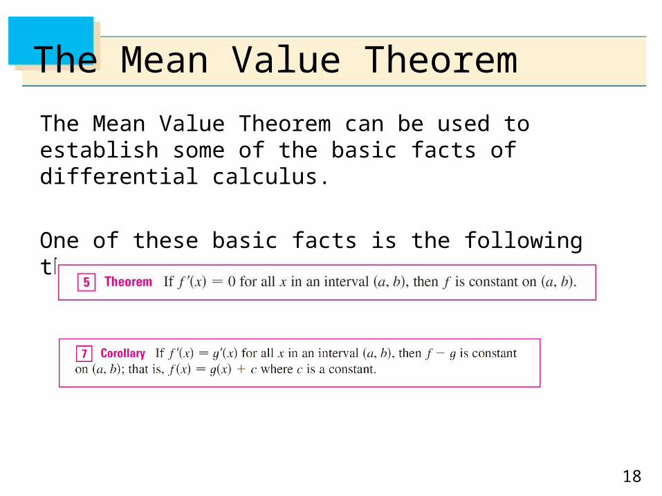
The Mean Value Theorem

The Mean Value Theorem can be used to establish some of the basic facts of differential calculus.

One of these basic facts is the following theorem.

19

The Mean Value Theorem

Note:

Care must be taken in applying Theorem 5. Let

The domain of f is D = {x | x ≠ 0} and f (x) = 0 for all x in D. But f is obviously not a constant function.

This does not contradict Theorem 5 because D is not an interval. Notice that f is constant on the interval (0, ) and also on the interval ( , 0).