Copyright © Cengage Learning. All rights reserved.

3 Differentiation Rules

Copyright © Cengage Learning. All rights reserved.

3.1Derivatives of Polynomials and

Exponential Functions

33

Derivatives of Polynomials and Exponential Functions

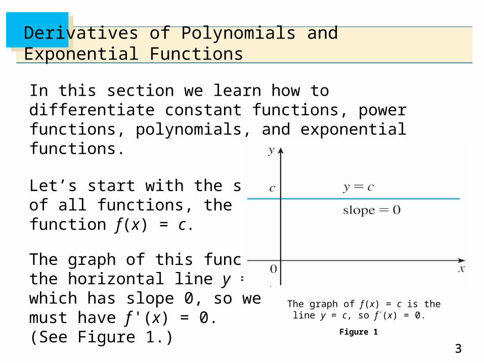
In this section we learn how to differentiate constant functions, power functions, polynomials, and exponential functions.

Let’s start with the simplestof all functions, the constant function f (x) = c.

The graph of this function isthe horizontal line y = c, which has slope 0, so we must have f '(x) = 0. (See Figure 1.)

Figure 1

The graph of f (x) = c is the line y = c, so f (x) = 0.

44

Derivatives of Polynomials and Exponential Functions

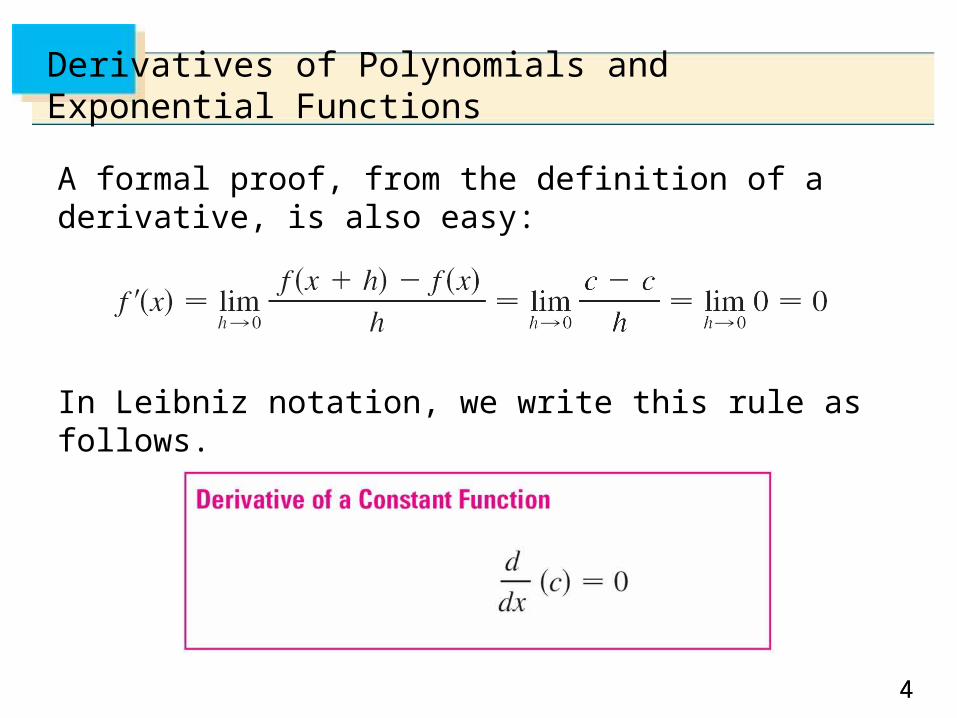
A formal proof, from the definition of a derivative, is also easy:

In Leibniz notation, we write this rule as follows.

55

Power Functions

66

Power Functions

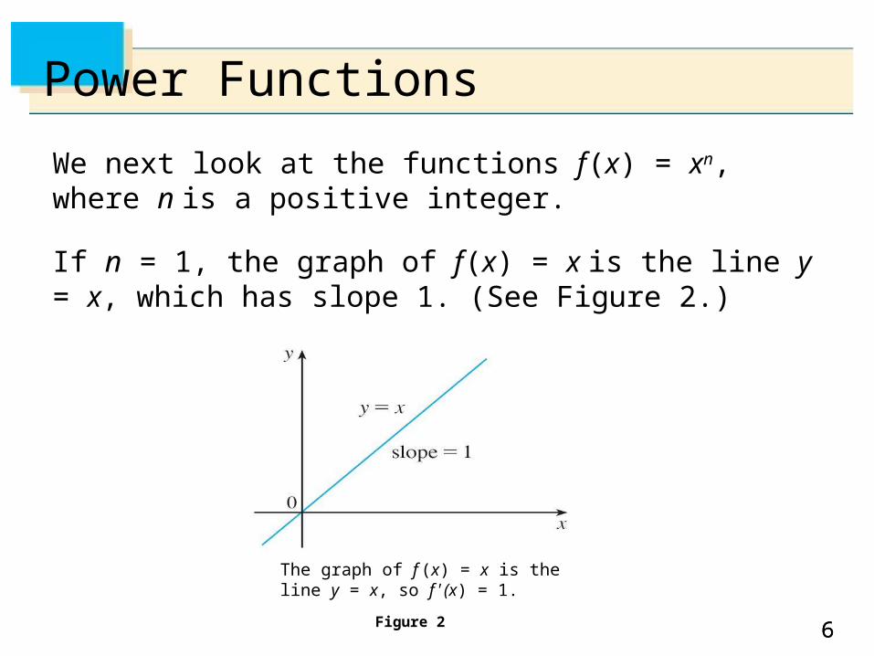
We next look at the functions f (x) = xn, where n is a positive integer.

If n = 1, the graph of f (x) = x is the line y = x, which has slope 1. (See Figure 2.)

Figure 2

The graph of f (x) = x is the line y = x, so f ' (x) = 1.

77

Power Functions

So

(You can also verify Equation 1 from the definition of a derivative.)

We have already investigated the cases n = 2 and n = 3. We found that

88

Power Functions

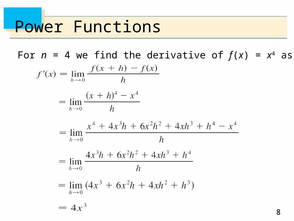
For n = 4 we find the derivative of f (x) = x4 as follows:

99

Power Functions

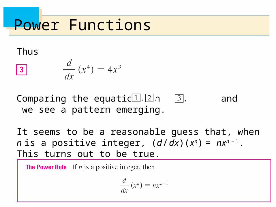
Thus

Comparing the equations in and we see a pattern emerging.

It seems to be a reasonable guess that, when n is a positive integer, (d / dx)(xn) = nxn

–

1. This turns out to be true.

1010

Example 1

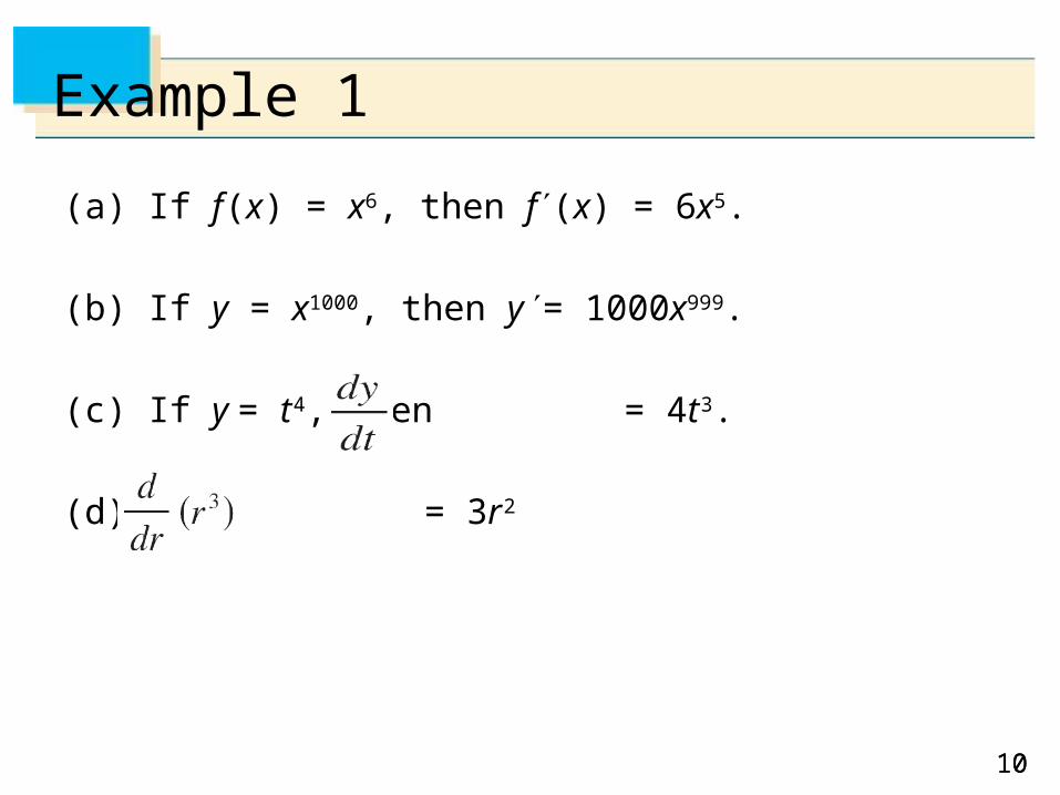
(a) If f (x) = x6, then f (x) = 6x5.

(b) If y = x1000, then y = 1000x999.

(c) If y = t

4, then = 4t

3.

(d) = 3r

2

1111

Power Functions

The Power Rule enables us to find tangent lines without having to resort to the definition of a derivative. It also enables us to find normal lines.

The normal line to a curve C at a point P is the line through P that is perpendicular to the tangent line at P.

1212

New Derivatives from Old

1313

New Derivatives from Old

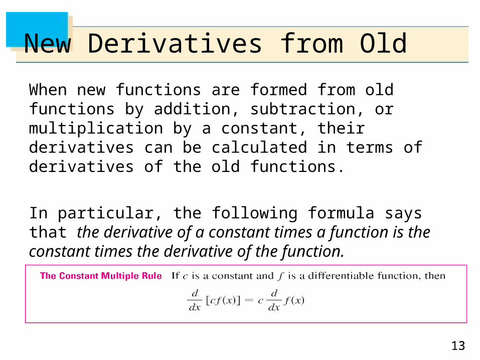
When new functions are formed from old functions by addition, subtraction, or multiplication by a constant, their derivatives can be calculated in terms of derivatives of the old functions.

In particular, the following formula says that the derivative of a constant times a function is the constant times the derivative of the function.

1414

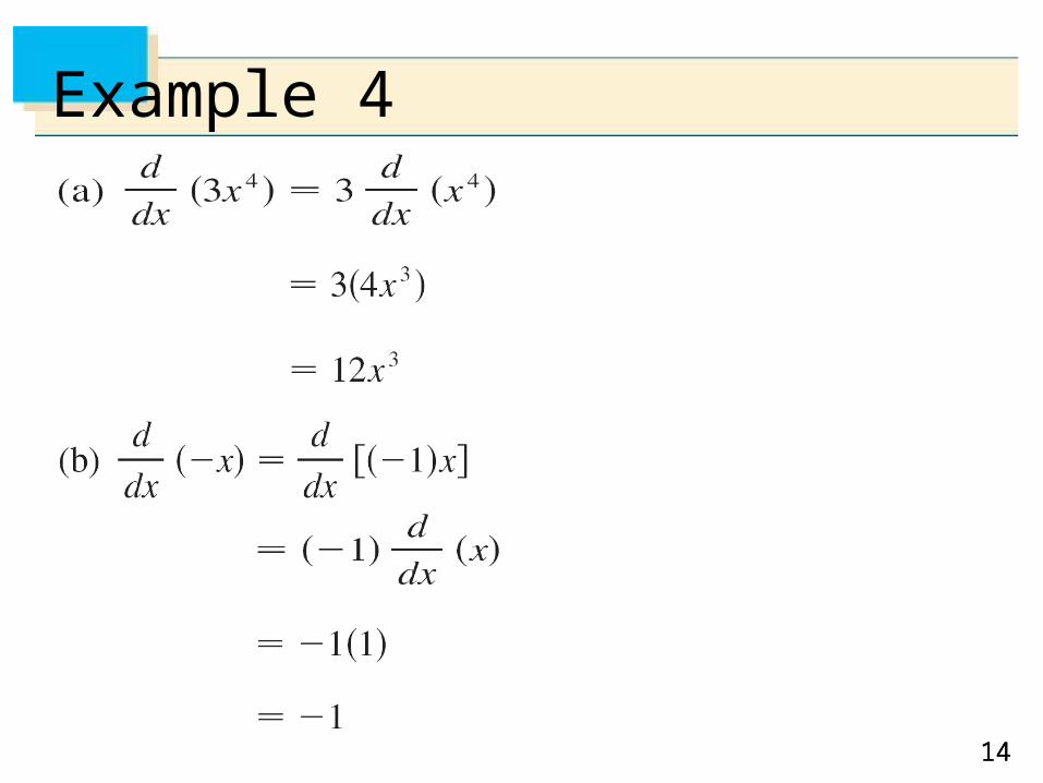
Example 4

1515

New Derivatives from Old

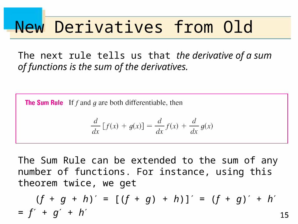
The next rule tells us that the derivative of a sum of functions is the sum of the derivatives.

The Sum Rule can be extended to the sum of any number of functions. For instance, using this theorem twice, we get

(f + g + h) = [(f + g) + h)] = (f + g) + h = f + g + h

1616

New Derivatives from Old

By writing f – g as f + (–1)g and applying the Sum Rule and the Constant Multiple Rule, we get the following formula.

The Constant Multiple Rule, the Sum Rule, and the Difference Rule can be combined with the Power Rule to differentiate any polynomial, as the following examples demonstrate.

1717

Exponential Functions

1818

Exponential Functions

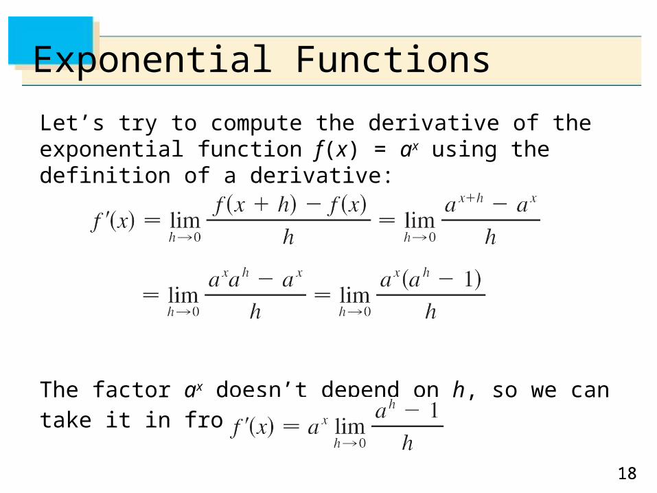
Let’s try to compute the derivative of the exponential function f (x) = ax using the definition of a derivative:

The factor ax doesn’t depend on h, so we can take it in front of the limit:

1919

Exponential Functions

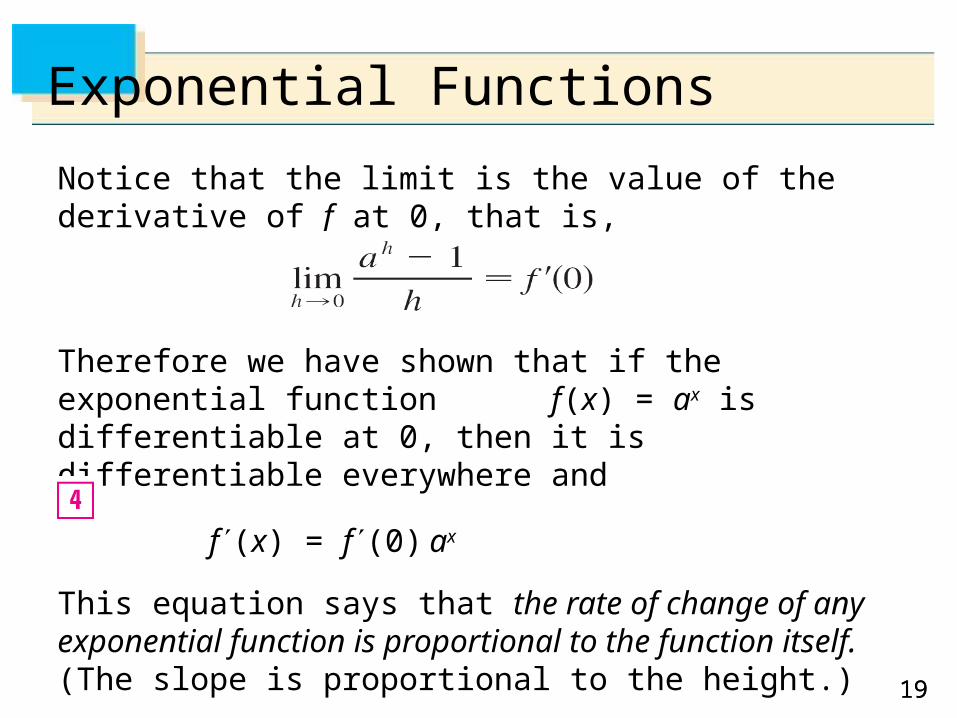
Notice that the limit is the value of the derivative of f at 0, that is,

Therefore we have shown that if the exponential function f (x) = ax is differentiable at 0, then it is differentiable everywhere and

f (x) = f (0) ax

This equation says that the rate of change of any exponential function is proportional to the function itself.(The slope is proportional to the height.)

2020

Exponential Functions

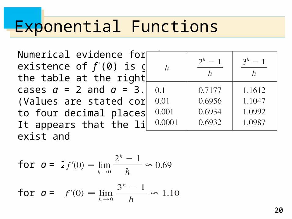
Numerical evidence for the existence of f (0) is given in the table at the right for the cases a = 2 and a = 3. (Values are stated correct to four decimal places.) It appears that the limits exist and

for a = 2,

for a = 3,

2121

Exponential Functions

In fact, it can be proved that these limits exist and, correct to six decimal places, the values are

Thus, from Equation 4, we have

Of all possible choices for the base a in Equation 4, the simplest differentiation formula occurs when f (0) = 1.

2222

Exponential Functions

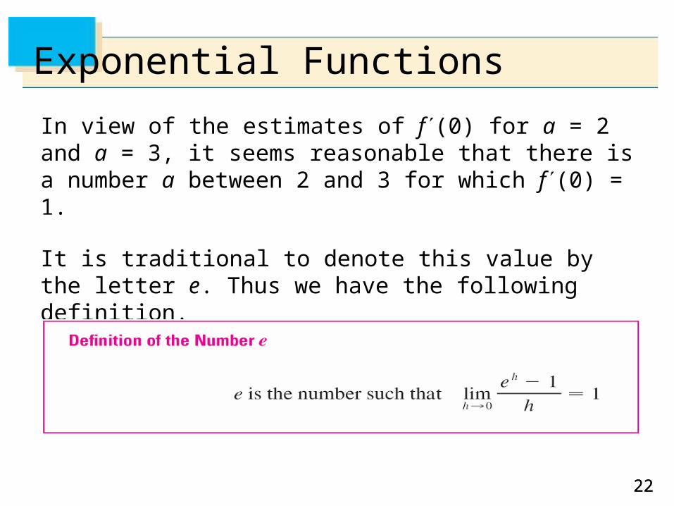
In view of the estimates of f (0) for a = 2 and a = 3, it seems reasonable that there is a number a between 2 and 3 for which f (0) = 1.

It is traditional to denote this value by the letter e. Thus we have the following definition.

2323

Exponential Functions

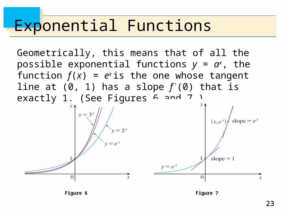
Geometrically, this means that of all the possible exponential functions y = ax, the function f (x) = ex is the one whose tangent line at (0, 1) has a slope f (0) that is exactly 1. (See Figures 6 and 7.)

Figure 6 Figure 7

2424

Exponential Functions

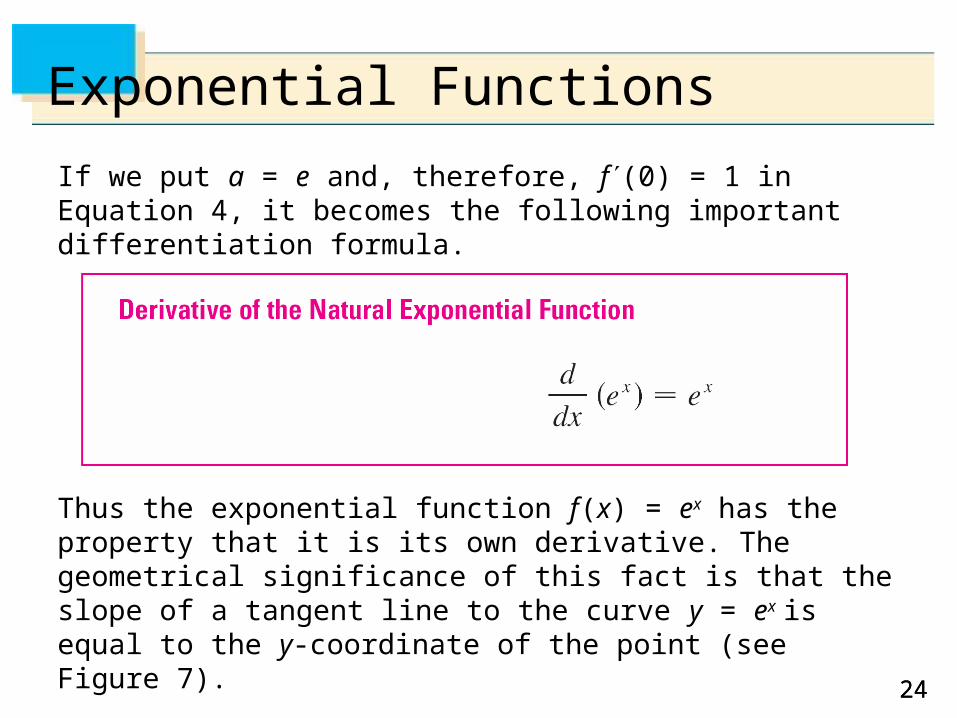
If we put a = e and, therefore, f (0) = 1 in Equation 4, it becomes the following important differentiation formula.

Thus the exponential function f (x) = ex has the property that it is its own derivative. The geometrical significance of this fact is that the slope of a tangent line to the curve y = ex is equal to the y-coordinate of the point (see Figure 7).

2525

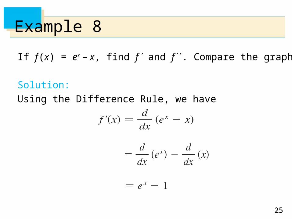
Example 8

If f (x) = ex – x, find f and f . Compare the graphs of f and f .

Solution:

Using the Difference Rule, we have

2626

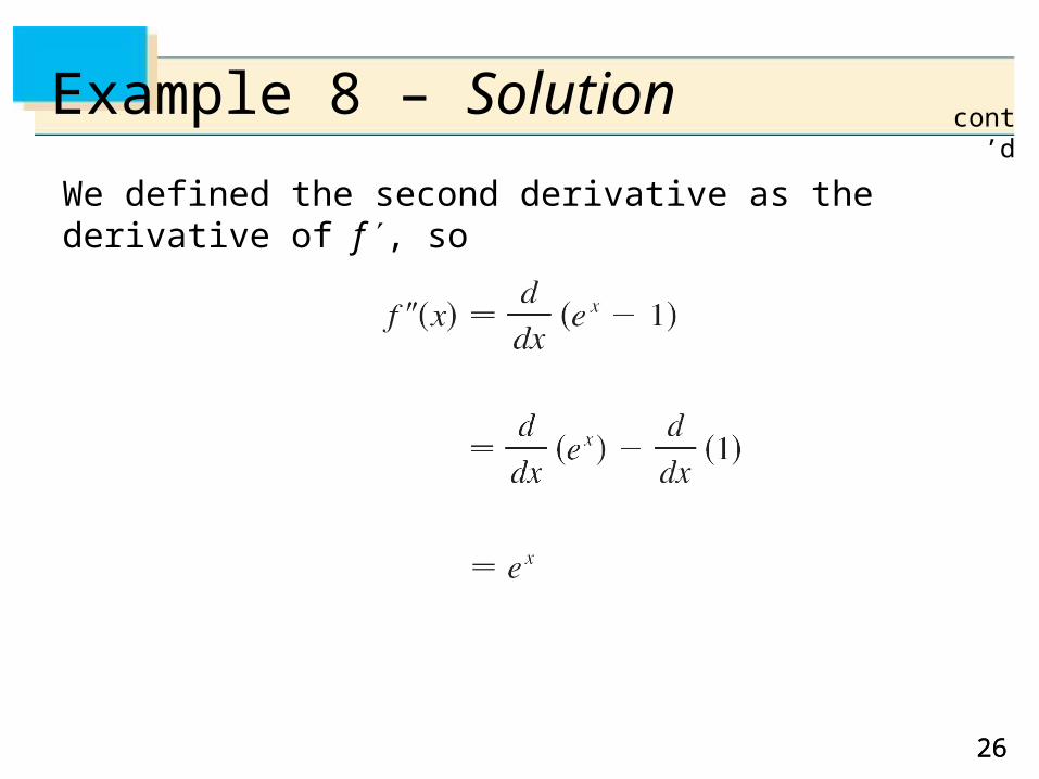
Example 8 – Solution

We defined the second derivative as the derivative of f , so

cont’d

2727

Example 8 – Solution

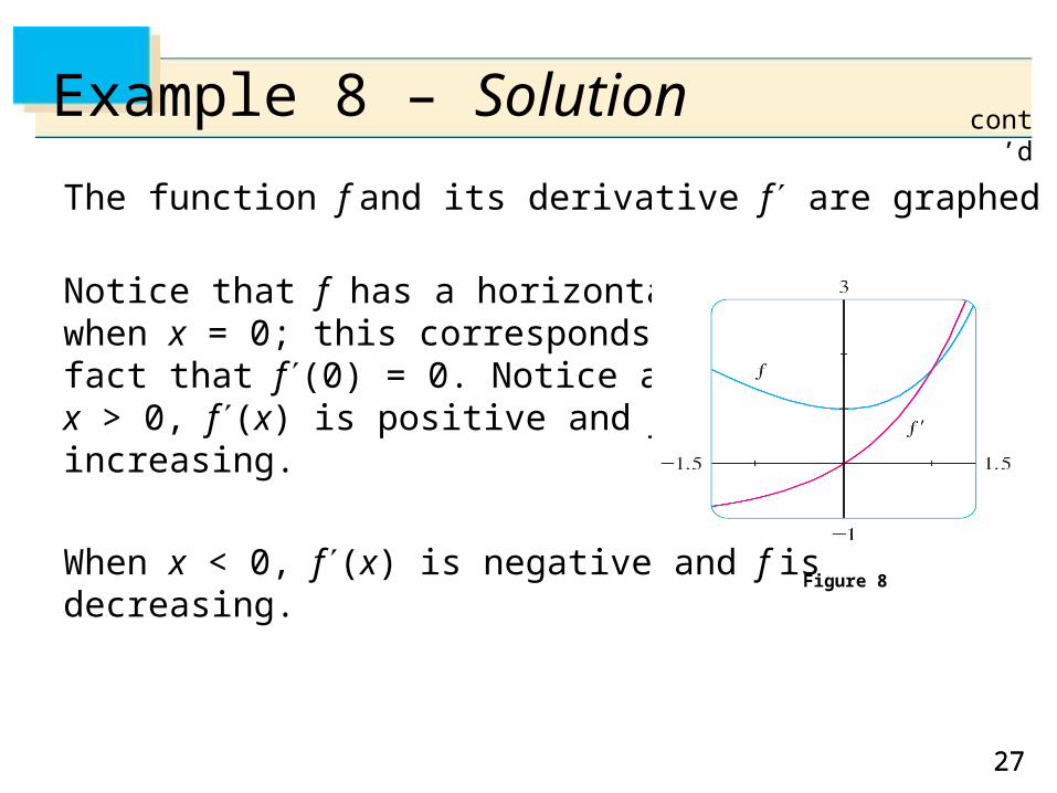
The function f and its derivative f are graphed in Figure 8.

Notice that f has a horizontal tangent when x = 0; this corresponds to the fact that f (0) = 0. Notice also that, for x > 0, f (x) is positive and f is increasing.

When x < 0, f (x) is negative and f is decreasing.

Figure 8

cont’d