Copyright

by

Martin Daniel Schatz

2015

The Dissertation Committee for Martin Daniel Schatz

certifies that this is the approved version of the following dissertation:

Distributed Tensor Computations:

Formalizing Distributions, Redistributions,

and Algorithm Derivation

Committee:

Robert A. van de Geijn, Supervisor

Tamara G. Kolda, Co-Supervisor

John F. Stanton

Keshav Pingali

Jeff R. Hammond

Don S. Batory

Distributed Tensor Computations:

Formalizing Distributions, Redistributions,

and Algorithm Derivation

by

Martin Daniel Schatz, B.S.C.S.; B.S.Ch.

Dissertation

Presented to the Faculty of the Graduate School of

The University of Texas at Austin

in Partial Fulfillment

of the Requirements

for the Degree of

Doctor of Philosophy

The University of Texas at Austin

December 2015

Dedicated to my mother.

Acknowledgments

Upon entering graduate school I knew that I wanted to conduct research related

to both chemistry and computer science. Ultimately, I focused my efforts in the

domain of tensor computations. It was due to Prof. Robert van de Geijn’s previous

experience, insights, and formal approach to the domain of high-performance dense

linear algebra that I was able to gain intuition to extend key ideas to the domain

of tensor computations. An initial theory was developed to express the intuition for

distributed tensor computations thanks to the countless hours spent at the white-

board discussing with Dr. Tze Meng Low. Once the initial theory was developed,

Dr. Devin Matthews provided the practical application to make the theory meaning-

ful. At this point, we could justify the madness and, thanks to Devin’s unflappable

demeanor, we understood the intricacies of the applications. It was then recognized

that DxTer would be an invaluable tool to use for optimizing such applications. As

DxTer is the product of Dr. Bryan Marker, we could start a true collaboration to

test the developed theory. After having explained the theory, Bryan encoded the

knowledge into DxTer, thereby giving us a way to test the theory. Without Bryan’s

tireless efforts, I would not have been able to finish this work as soon as I have.

Unfortunately, only the handful of people mentioned understood the theory and

notation. It is thanks to Dr.Tamara G. Kolda’s meticulous eye for detail that the

notation and theory has been refined into what it is today. Because of these efforts,

v

I would like to extend my deepest thanks to Robert, Tze Meng, Devin, Bryan, and

Tammy.

In addition to the efforts associated with this dissertation, I am fortunate to have had

both Robert and Tammy as my mentors. Not only have they guided me throughout

my career as a graduate student, including preparing for the future and exposing me

to different aspects of being a researcher, but they have also helped me how to better

convey my ideas through writing, which is no simple task (as anyone who knows me

can attest to). It is only through their constant encouragement and pressure to do

better that I have been able to achieve all that I have. Once again, thank you.

Finally, I cannot go without acknowledging everyone I consider family (you know

who you are). In particular, I would like to thank my brother Philip Schatz and

my wife Erin Ballou. Philip always managed to do something zany, providing me

needed reprieve from the stresses of this work, while at the same time (okay different

time) showing me how fortunate I am to have him as a brother. And Erin, she is my

rock. Whenever things looked impossible, Erin was there to make sure I knew that

the impossible could be overcome. I have asked more from her than I could ever ask

anyone, and I hope to be able to at least come close to making good on those loans.

I am glad that I can finally begin repaying her for everything she has done for me

during this long process. From the bottom of my heart, thank you all.

Martin Daniel Schatz

The University of Texas at Austin

December 2015

vi

Distributed Tensor Computations:

Formalizing Distributions, Redistributions,

and Algorithm Derivation

Publication No.

Martin Daniel Schatz, Ph.D.

The University of Texas at Austin, 2015

Supervisor: Robert A. van de Geijn

Co-Supervisor: Tamara G. Kolda

A goal of computer science is to develop practical methods to automate tasks that are

otherwise too complex or tedious to perform manually. Complex tasks can include

determining a practical algorithm and creating the associated implementation for a

given problem specification. Goal-oriented programming can make this systematic.

Therefore, we can rely on automated tools to create implementations by expressing

vii

the task of creating implementations in terms of goal-oriented programming. To do

so, pertinent knowledge must be encoded which requires a notation and language

to define relevant abstractions.

This dissertation focuses on distributed-memory parallel tensor computations arising

from computational chemistry. Specifically, we focus on applications based on the

tensor contraction operation of dense, non-symmetric tensors. Creating an efficient

algorithm for a given problem specification in this domain is complex; creating an

optimized implementation of a developed algorithm is even more complex, tedious,

and error-prone. To this end, we encode pertinent knowledge for distributed-memory

parallel algorithms for tensor contractions of dense non-symmetric tensors. We do

this by developing a notation for data distribution and redistribution that exposes a

systematic procedure for deriving a family of algorithms for this operation for which

efficient implementations exist.

We validate the developed ideas by implementing them in the Redistribution Op-

erations and Tensor Expressions application programming interface (ROTE API)

and encoding them into an automated system, DxTer, for systematically generat-

ing efficient implementations from problem specifications. Experiments performed

on the IBM Blue Gene/Q and Cray XC30 architectures testing generated imple-

mentations for the spin-adapted coupled cluster singles and doubles method from

computational chemistry demonstrate impact both in terms of performance and

storage requirements.

viii

Contents

Acknowledgments v

Abstract vii

Glossary of Notation xiv

Chapter 1 Introduction 1

1.1 Motivation and Goals . . . . . . . . . . . . . . . . . . . . . . . . . . 2

1.2 Solution . . . . . . . . . . . . . . . . . . . . . . . . . . . . . . . . . . 5

1.3 Background . . . . . . . . . . . . . . . . . . . . . . . . . . . . . . . . 6

1.3.1 Parallel Matrix-Matrix Multiplication . . . . . . . . . . . . . 6

1.3.2 Design-by-Transformation for Matrix Computations . . . . . 7

1.4 Contributions . . . . . . . . . . . . . . . . . . . . . . . . . . . . . . . 8

1.5 Outline of the Dissertation . . . . . . . . . . . . . . . . . . . . . . . . 9

Chapter 2 Notation 11

2.1 Preliminaries . . . . . . . . . . . . . . . . . . . . . . . . . . . . . . . 11

2.1.1 Tensors . . . . . . . . . . . . . . . . . . . . . . . . . . . . . . 11

2.1.2 Processing Mesh . . . . . . . . . . . . . . . . . . . . . . . . . 12

ix

2.1.3 Ordered Sets . . . . . . . . . . . . . . . . . . . . . . . . . . . 13

2.1.4 Index Conversion . . . . . . . . . . . . . . . . . . . . . . . . . 15

2.2 The Tensor Contraction Operation . . . . . . . . . . . . . . . . . . . 19

2.2.1 Binary Tensor Contraction . . . . . . . . . . . . . . . . . . . 19

2.2.2 Unary Tensor Contractions . . . . . . . . . . . . . . . . . . . 21

2.3 Data Distributions . . . . . . . . . . . . . . . . . . . . . . . . . . . . 21

2.3.1 Elemental-cyclic Distributions for 1-D Data . . . . . . . . . . 22

2.3.2 Tensor Mode and Tensor Distributions . . . . . . . . . . . . . 27

2.3.3 Advanced Tensor Distributions . . . . . . . . . . . . . . . . . 30

2.3.4 Tensor Distribution Constraints . . . . . . . . . . . . . . . . . 33

2.4 Collective Communications . . . . . . . . . . . . . . . . . . . . . . . 33

2.5 Data Redistributions . . . . . . . . . . . . . . . . . . . . . . . . . . . 38

2.5.1 Example: Stationary C Parallel Matrix Multiplication . . . . 39

2.5.2 Example: Stationary A Parallel Matrix Multiplication . . . . 45

2.5.3 Example: Allreduce and Gather-to-one . . . . . . . . . . . . . 51

2.5.4 Collective Redistribution Rules . . . . . . . . . . . . . . . . . 53

2.6 Summary . . . . . . . . . . . . . . . . . . . . . . . . . . . . . . . . . 58

Chapter 3 Algorithm Derivation 59

3.1 Preliminaries . . . . . . . . . . . . . . . . . . . . . . . . . . . . . . . 60

3.1.1 Approach . . . . . . . . . . . . . . . . . . . . . . . . . . . . . 60

3.1.2 Distributed Template . . . . . . . . . . . . . . . . . . . . . . 62

3.2 Example: Stationary C Algorithms . . . . . . . . . . . . . . . . . . . 64

3.2.1 Derivation . . . . . . . . . . . . . . . . . . . . . . . . . . . . . 65

3.2.2 Blocking . . . . . . . . . . . . . . . . . . . . . . . . . . . . . . 69

3.2.3 Observations . . . . . . . . . . . . . . . . . . . . . . . . . . . 70

x

3.3 Example: Stationary A Algorithms . . . . . . . . . . . . . . . . . . . 71

3.3.1 Derivation . . . . . . . . . . . . . . . . . . . . . . . . . . . . . 71

3.3.2 Observations . . . . . . . . . . . . . . . . . . . . . . . . . . . 76

3.4 A Systematic Procedure for Deriving Stationary Algorithms . . . . . 76

3.5 Summary . . . . . . . . . . . . . . . . . . . . . . . . . . . . . . . . . 78

Chapter 4 Optimizing Data Movement 79

4.1 Global Data Movement . . . . . . . . . . . . . . . . . . . . . . . . . 80

4.1.1 Motivating Example . . . . . . . . . . . . . . . . . . . . . . . 81

4.1.2 Preliminaries . . . . . . . . . . . . . . . . . . . . . . . . . . . 84

4.1.3 Balancing Redistributions . . . . . . . . . . . . . . . . . . . . 86

4.1.4 Exploiting Processing Mesh Structure . . . . . . . . . . . . . 90

4.2 Local Data Movement . . . . . . . . . . . . . . . . . . . . . . . . . . 95

4.2.1 Motivating Example . . . . . . . . . . . . . . . . . . . . . . . 95

4.2.2 Generalization . . . . . . . . . . . . . . . . . . . . . . . . . . 98

4.3 Summary . . . . . . . . . . . . . . . . . . . . . . . . . . . . . . . . . 99

Chapter 5 Implementation and Experimental Results 100

5.1 Coupled Cluster Singles and Doubles Method (CCSD) . . . . . . . . 101

5.1.1 Computational Chemistry Background . . . . . . . . . . . . . 102

5.1.2 The Specific Formulation Studied . . . . . . . . . . . . . . . . 103

5.2 The Redistribution Operations and Tensor Expressions (ROTE) API 105

5.3 Design-by-Transformation (DxT) and DxTer . . . . . . . . . . . . . 108

5.3.1 Background . . . . . . . . . . . . . . . . . . . . . . . . . . . . 108

5.3.2 DxT and This Dissertation . . . . . . . . . . . . . . . . . . . 111

5.4 Experimental Results . . . . . . . . . . . . . . . . . . . . . . . . . . . 112

xi

5.4.1 Target Architectures . . . . . . . . . . . . . . . . . . . . . . . 112

5.4.2 IBM Blue Gene/Q Experiments . . . . . . . . . . . . . . . . . 113

5.4.3 Cray XC30 Experiments . . . . . . . . . . . . . . . . . . . . . 116

5.4.4 The Importance of Blocking . . . . . . . . . . . . . . . . . . . 120

5.4.5 Weak Scalability Experiments . . . . . . . . . . . . . . . . . . 123

5.5 Summary . . . . . . . . . . . . . . . . . . . . . . . . . . . . . . . . . 126

Chapter 6 Related Work 127

6.1 Tensor Contraction Engine (TCE) . . . . . . . . . . . . . . . . . . . 127

6.2 Advanced Concepts in Electronic Structure III (ACES III) . . . . . . 129

6.3 Cyclops Tensor Framework (CTF) . . . . . . . . . . . . . . . . . . . 130

6.4 RRR and The Contraction Algorithm for Symmetric Tensors (CAST) 132

6.5 Elemental . . . . . . . . . . . . . . . . . . . . . . . . . . . . . . . . . 133

6.6 Summary . . . . . . . . . . . . . . . . . . . . . . . . . . . . . . . . . 134

Chapter 7 Conclusion 135

7.1 Contributions . . . . . . . . . . . . . . . . . . . . . . . . . . . . . . . 135

7.1.1 A Notation for Data Distributions of Tensors . . . . . . . . . 136

7.1.2 A Notation for Data Redistributions of Tensors . . . . . . . . 136

7.1.3 A Generalization of Transformations for Improving Performance137

7.1.4 A Systematic Method for Algorithm Derivation . . . . . . . . 137

7.1.5 An API for Distributed Tensor Library Development . . . . . 137

7.1.6 An Advancement in State-of-the-Art Tensor Computations . 138

7.1.7 A New Case Study for DxTer . . . . . . . . . . . . . . . . . . 138

7.2 Future Work . . . . . . . . . . . . . . . . . . . . . . . . . . . . . . . 138

7.2.1 Symmetry . . . . . . . . . . . . . . . . . . . . . . . . . . . . . 139

xii

7.2.2 Sparsity . . . . . . . . . . . . . . . . . . . . . . . . . . . . . . 139

7.2.3 Additional Families of Algorithms . . . . . . . . . . . . . . . 139

7.2.4 Additional Data Distributions . . . . . . . . . . . . . . . . . . 140

7.2.5 Generalizations of the Derivation Process . . . . . . . . . . . 140

7.2.6 Additional Optimizing Transformations . . . . . . . . . . . . 140

7.2.7 Additional Tensor Operations . . . . . . . . . . . . . . . . . . 141

7.2.8 Heuristics for Reducing the Space of Implementations . . . . 141

7.2.9 Aiding Automated Tools . . . . . . . . . . . . . . . . . . . . . 141

Appendices 142

Appendix A Proofs of Redistribution Rules 143

A.1 Proofs of Correctness Strategy . . . . . . . . . . . . . . . . . . . . . 143

A.2 Lemmas . . . . . . . . . . . . . . . . . . . . . . . . . . . . . . . . . . 146

A.3 Proofs of Correctness . . . . . . . . . . . . . . . . . . . . . . . . . . . 148

A.3.1 All-to-all . . . . . . . . . . . . . . . . . . . . . . . . . . . . . 148

A.3.2 Scatter . . . . . . . . . . . . . . . . . . . . . . . . . . . . . . 152

A.3.3 Gather-to-one . . . . . . . . . . . . . . . . . . . . . . . . . . . 154

A.3.4 Permutation . . . . . . . . . . . . . . . . . . . . . . . . . . . 155

A.3.5 Others . . . . . . . . . . . . . . . . . . . . . . . . . . . . . . . 158

A.4 Proofs of Balance . . . . . . . . . . . . . . . . . . . . . . . . . . . . . 160

A.4.1 All-to-all . . . . . . . . . . . . . . . . . . . . . . . . . . . . . 160

Bibliography 163

xiii

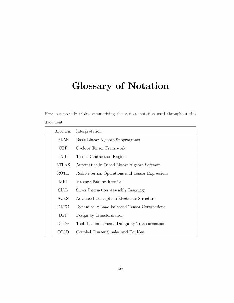
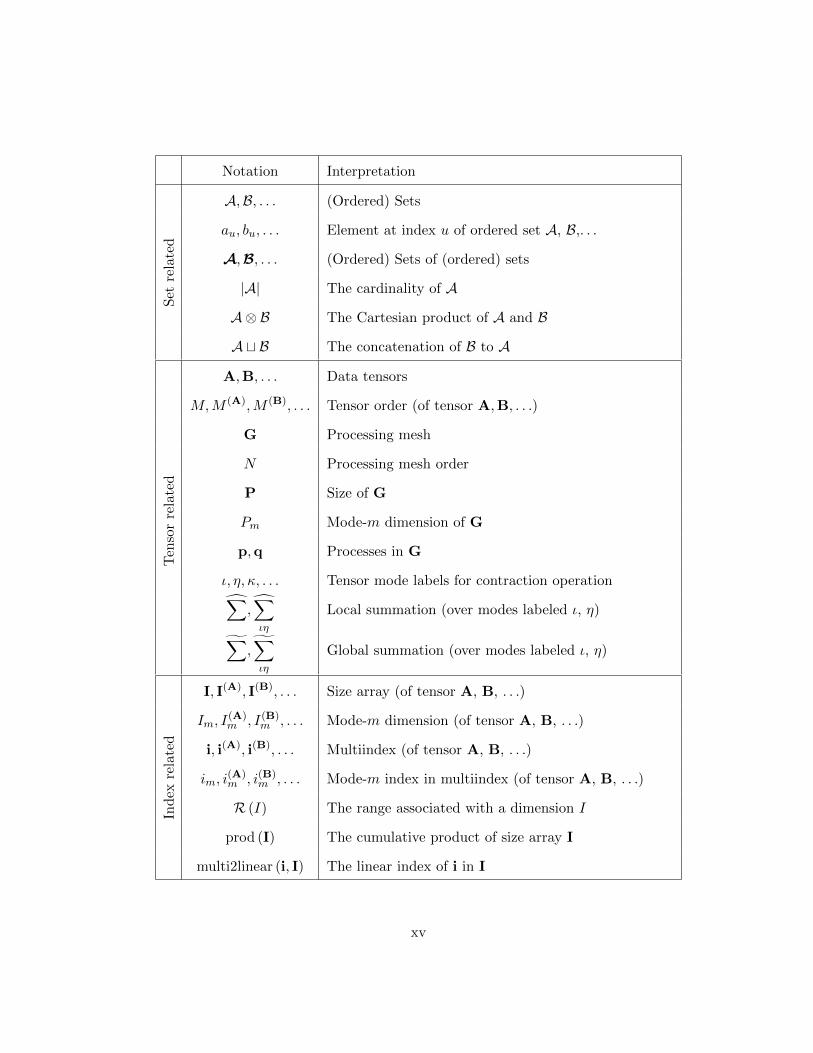
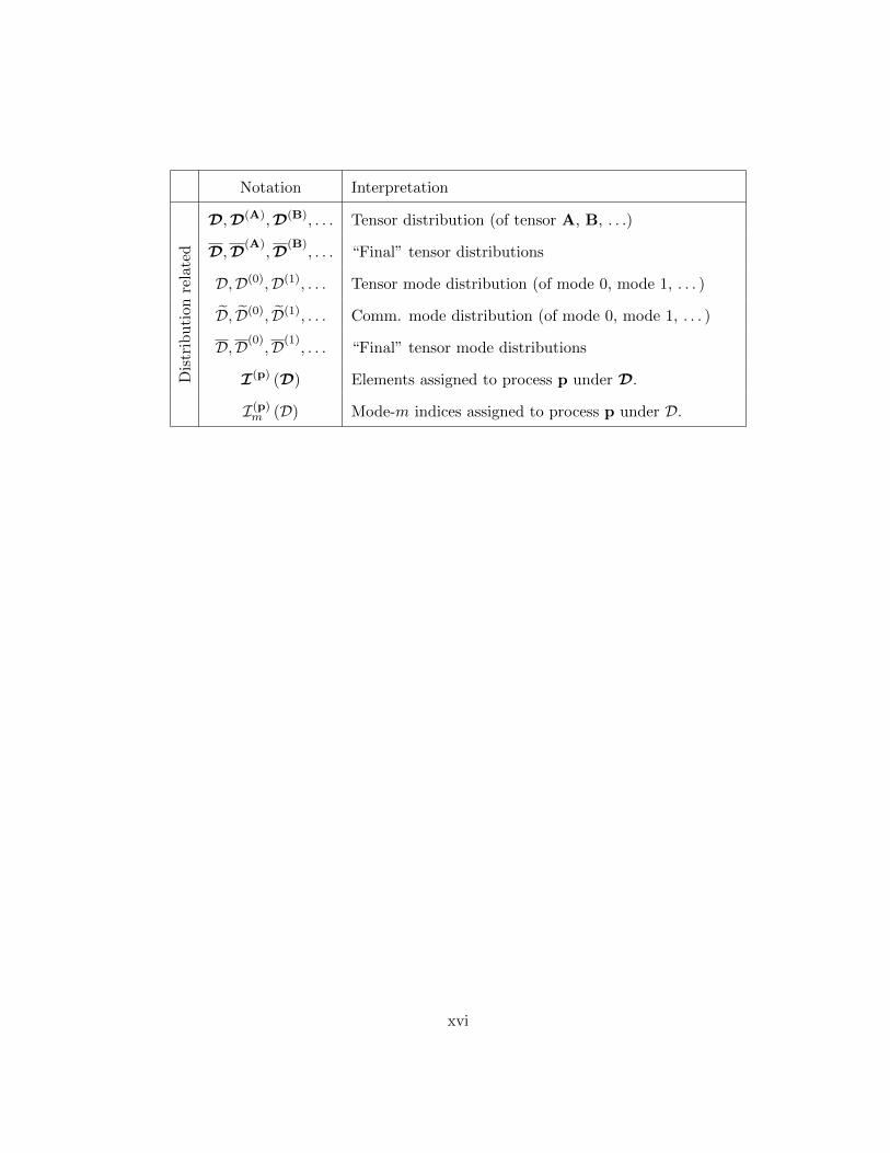
Glossary of Notation

Here, we provide tables summarizing the various notation used throughout this

document.

Acronym Interpretation

BLAS Basic Linear Algebra Subprograms

CTF Cyclops Tensor Framework

TCE Tensor Contraction Engine

ATLAS Automatically Tuned Linear Algebra Software

ROTE Redistribution Operations and Tensor Expressions

MPI Message-Passing Interface

SIAL Super Instruction Assembly Language

ACES Advanced Concepts in Electronic Structure

DLTC Dynamically Load-balanced Tensor Contractions

DxT Design by Transformation

DxTer Tool that implements Design by Transformation

CCSD Coupled Cluster Singles and Doubles

xiv

Notation InterpretationS

etre

late

d

A,B, . . . (Ordered) Sets

au, bu, . . . Element at index u of ordered set A, B,. . .

A,B, . . . (Ordered) Sets of (ordered) sets

|A| The cardinality of A

A⊗ B The Cartesian product of A and B

A t B The concatenation of B to A

Ten

sor

rela

ted

A,B, . . . Data tensors

M,M (A),M (B), . . . Tensor order (of tensor A,B, . . .)

G Processing mesh

N Processing mesh order

P Size of G

Pm Mode-m dimension of G

p,q Processes in G

ι, η, κ, . . . Tensor mode labels for contraction operation∑,∑ιη

Local summation (over modes labeled ι, η)∑,∑ιη

Global summation (over modes labeled ι, η)

Ind

exre

late

d

I, I(A), I(B), . . . Size array (of tensor A, B, . . .)

Im, I(A)m , I(B)

m , . . . Mode-m dimension (of tensor A, B, . . .)

i, i(A), i(B), . . . Multiindex (of tensor A, B, . . .)

im, i(A)m , i(B)

m , . . . Mode-m index in multiindex (of tensor A, B, . . .)

R (I) The range associated with a dimension I

prod (I) The cumulative product of size array I

multi2linear (i, I) The linear index of i in I

xv

Notation InterpretationD

istr

ibu

tion

rela

ted

D,D(A),D(B), . . . Tensor distribution (of tensor A, B, . . .)

D,D(A),D(B)

, . . . “Final” tensor distributions

D,D(0),D(1), . . . Tensor mode distribution (of mode 0, mode 1, . . . )

D, D(0), D(1), . . . Comm. mode distribution (of mode 0, mode 1, . . . )

D,D(0),D(1)

, . . . “Final” tensor mode distributions

I(p) (D) Elements assigned to process p under D.

I(p)m (D) Mode-m indices assigned to process p under D.

xvi

Chapter 1

Introduction

For dense linear algebra, it has already been shown that carefully structured abstrac-

tions support the development of implementations that achieve high performance on

distributed-memory architectures [18, 65, 86]. Tensor contractions, the generaliza-

tion of matrix-matrix multiplication to higher-dimensional objects, are inherently

more difficult operations to optimize due to the number of algorithmic variants that

can, and as we demonstrate, need to be considered, making a full optimization

daunting, even to an expert.

The thesis of this work is that a notation can be defined for data distributions and

redistributions that exposes a systematic procedure for deriving parallel algorithms

with high-performance implementations for the tensor contraction operation of dense

non-symmetric tensors. In doing so, pertinent domain knowledge is consolidated

into a formal language that facilitates the automatic generation of algorithms with

high-performance implementations for individual and, more importantly, a series

of tensor contractions. These techniques advance the state of the art in computer

1

science by providing the foundation for encoding pertinent knowledge in the domain

of distributed-memory parallel tensor computations. Additionally, these techniques

advance the state of the art in computational chemistry as implementations for the

spin-adapted coupled cluster singles and doubles method (CCSD) are developed that

require at most half the available memory for workspace and attain performance that

improves upon state of the art.

1.1 Motivation and Goals

The goal of any computational method designed for a distributed-memory archi-

tecture is to effectively utilize the available processing elements (processes) to col-

lectively perform a computation. For the domain of dense linear algebra, both

theoretical and practical approaches have been developed that achieve high per-

formance on distributed-memory architectures while simultaneously reducing the

storage needed for workspace [2, 18, 34, 49, 65, 79, 86, 87]. For each of these, the

relationship between the data distribution and the developed algorithm must be

considered in conjunction. This is necessary not only to ensure that data is effi-

ciently distributed and redistributed among processes, but also to ensure that local

computations performed by each process are efficient [73].

Tensors are multidimensional arrays and can be considered generalizations of ma-

trices. The order of a tensor is the number of ways or dimensions that it represents.

We say a tensor is higher-order if its order is greater than two. Tensor contrac-

tions are a generalization of matrix-matrix multiplication and are, for example, at

the heart of methods in computational chemistry [7, 62, 66]. As we discuss in the

next section, the challenge in developing efficient implementations for tensor con-

2

tractions stems from the increased number of data distributions and algorithmic

variants available.

The simplest approach to computing a tensor contraction is to rearrange the data,

express the computation in terms of a matrix-matrix multiplication, and leverage

previous work on parallelizing that simpler operation. Unfortunately, in doing so,

the multiway structure of the operation is inherently lost, thereby reducing the

opportunities for improving performance and/or limiting workspace requirements.

Instead, in this work, we exploit the similarities between tensor contractions and

matrix-matrix multiplication, allowing us to extend ideas used for matrix-matrix

multiplication [70, 72, 80, 81].

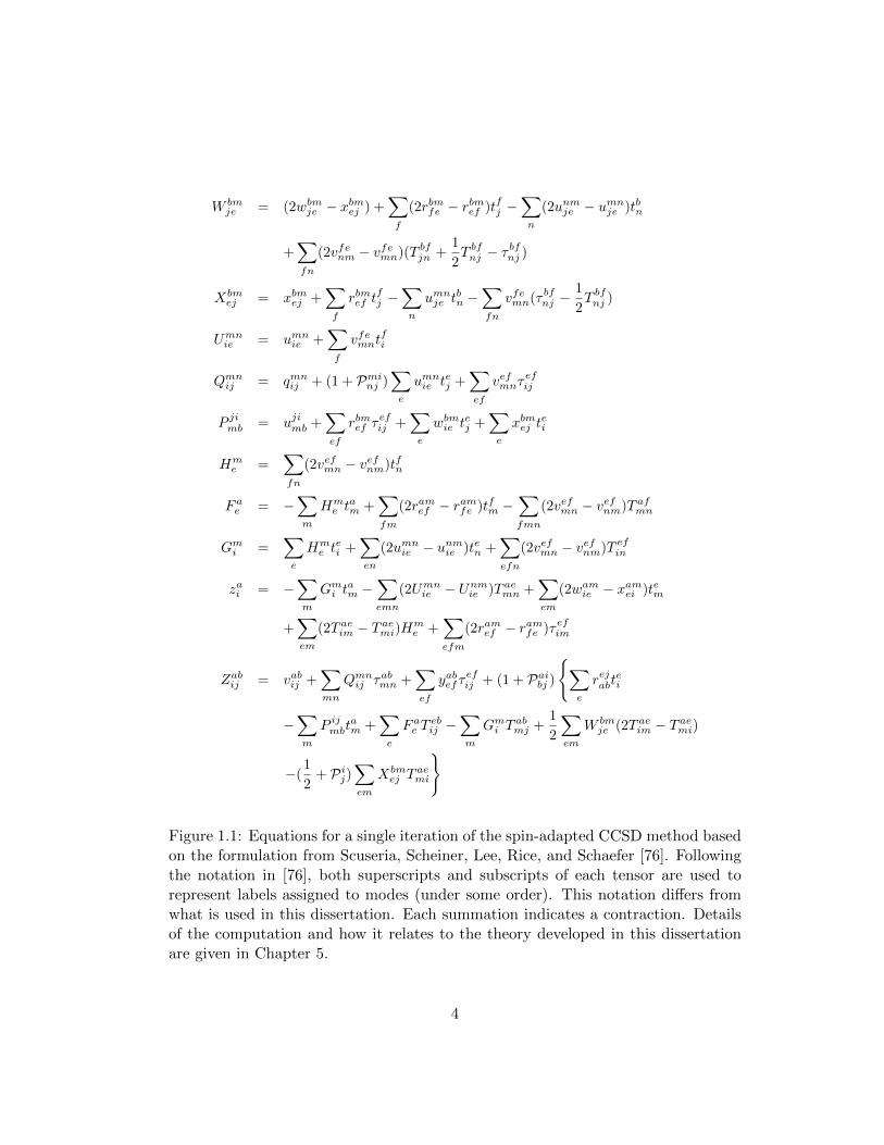
Many important computations in quantum chemistry can be expressed as a long se-

ries of contractions [47, 62, 66]. For example, Figure 1.1 depicts the set of equations

that define the CCSD application used as a motivating example in this work. We

discuss how to interpret the depicted equations in Section 2.2 and Section 5.1. For

now it is only necessary to understand that every instance of a summation in Fig-

ure 1.1 corresponds to a separate tensor contraction involving dense non-symmetric

tensors. As the goal is to optimize the entire computation, an expert has to con-

sider how to optimize all contractions in conjunction with one another in terms

of both communication and computation. This quickly becomes daunting. The

ideal solution is to automate this process; however, for automation to be possible, a

well-defined language that expresses pertinent information must be designed.

With a well-defined language that expresses the relationship between data distri-

bution, data redistribution, and the structure of the parallel algorithms used for

computation, we can reason about optimizing an entire series of contractions as all

steps involved are some combination of data redistribution or local computation.

3

W bmje = (2wbm

je − xbmej ) +∑f

(2rbmfe − rbmef )tfj −∑n

(2unmje − umnje )tbn

+∑fn

(2vfenm − vfemn)(T bfjn +

1

2T bfnj − τ

bfnj )

Xbmej = xbmej +

∑f

rbmef tfj −

∑n

umnje t

bn −

∑fn

vfemn(τ bfnj −1

2T bfnj )

Umnie = umn

ie +∑f

vfemntfi

Qmnij = qmn

ij + (1 + Pminj )

∑e

umnie tej +

∑ef

vefmnτefij

P jimb = ujimb +

∑ef

rbmef τefij +

∑e

wbmie t

ej +

∑e

xbmej tei

Hme =

∑fn

(2vefmn − vefnm)tfn

F ae = −

∑m

Hme t

am +

∑fm

(2ramef − ramfe )tfm −∑fmn

(2vefmn − vefnm)T afmn

Gmi =

∑e

Hme t

ei +

∑en

(2umnie − unmie )ten +

∑efn

(2vefmn − vefnm)T efin

zai = −∑m

Gmi t

am −

∑emn

(2Umnie − Unm

ie )T aemn +

∑em

(2wamie − xamei )tem

+∑em

(2T aeim − T ae

mi)Hme +

∑efm

(2ramef − ramfe )τefim

Zabij = vabij +

∑mn

Qmnij τabmn +

∑ef

yabefτefij + (1 + Pai

bj )

{∑e

rejabtei

−∑m

P ijmbt

am +

∑e

F ae T

ebij −

∑m

Gmi T

abmj +

1

2

∑em

W bmje (2T ae

im − T aemi)

−(1

2+ Pi

j)∑em

Xbmej T

aemi

}

Figure 1.1: Equations for a single iteration of the spin-adapted CCSD method basedon the formulation from Scuseria, Scheiner, Lee, Rice, and Schaefer [76]. Followingthe notation in [76], both superscripts and subscripts of each tensor are used torepresent labels assigned to modes (under some order). This notation differs fromwhat is used in this dissertation. Each summation indicates a contraction. Detailsof the computation and how it relates to the theory developed in this dissertationare given in Chapter 5.

4

By associating costs with each operation defined in the developed language, an au-

tomated system can make intelligent decisions about how applications should be

implemented. In this dissertation, we advance the state of the art towards achieving

this goal of automation.

As we discuss in related works (Chapter 6), recent advances that provide efficient

implementations for applications based on tensor computations are typically limited

to considering a single contraction at a time. However, many of these works support

tensor contractions involving sparse tensors or dense tensors with internal structure

such as symmetry. When restricted to applications based on contractions of dense,

non-symmetric tensors, this work differs in that it can optimize across a series of

contractions when designing the algorithms and associated implementations. This is

perhaps the most important difference of our work to that of other approaches.

1.2 Solution

We develop a notation that encodes a class of distributions of tensor data on a

multidimensional processing mesh as well as a set of redistributions that are directly

associated with various collective communications. With this notation, we expose

a systematic approach for deriving families of high-performance algorithms for an

arbitrary series of tensor contraction operations, thereby significantly reducing the

number of choices needed to be made by an expert (human or mechanical).

By encoding the structure of the algorithms and the necessary communications using

the same notation, decisions that normally would be made by an error-prone human

can be automated. With automated tools creating the implementations, one can

trust the correct optimizations to be applied wherever appropriate.

5

1.3 Background

Here we briefly discuss relevant history of parallel matrix-matrix multiplication as

well as the Design-by-Transformation approach to software engineering (DxT). This

provides the necessary background for the ideas developed in this document.

1.3.1 Parallel Matrix-Matrix Multiplication

Distributed-memory parallel algorithms for matrix-matrix multiplication, C = AB,

have a long and rich history. Cannon’s algorithm [15], the earliest such algorithm, is

based on a block distribution of elements and point-to-point communications that it-

eratively cycle blocks of both input matrices, A and B, among processes, computing

contributions to the result, C, at every iteration. Cannon’s algorithm is sometimes

referred to as the “roll-roll multiply” algorithm as blocks of both inputs A and B

are cycled during the computation. Later, Fox et al. [27] developed an algorithm,

sometimes called Fox’s algorithm, that relies on the broadcast collective to commu-

nicate one of the two input matrices and a point-to-point communication for the

other. For this reason, Fox’s algorithm is sometimes referred to as the “broadcast-

roll multiply” algorithm. Both algorithms target square processing meshes and are

difficult to generalize to non-square configurations [19, 38, 39].

In the 1990s, algorithms were developed that improved upon both Cannon’s and

Fox’s algorithms. Agarwal et al. [3], an algorithm is developed based on the all-

gather collective communication1 using a cyclic distribution of data. The scalable

universal matrix multiplication algorithm (SUMMA) [87], developed in 1997, casts

redistributions of both input operands in terms of broadcast collectives. One impor-

1communication involving groups of processes

6

tant contribution of [87] is the development of related algorithms for the different

transpose variants of matrix-matrix multiplication, developing a step towards a fam-

ily of algorithms. Gunnels et al. [30], a family of algorithms based on the idea of

holding one operand “stationary” is developed based on broadcast, allgather, scatter,

reduce-to-one, and gather-to-one collectives for communication. Creating families

of algorithms allows selection of an algorithm that is most suitable for the problem

of interest.

Following these previous works based on two-dimensional processing meshes, it was

discovered that better theoretical and practical results could be achieved for matrix-

matrix multiplication on a three-dimensional processing mesh [2, 41, 79]. The sys-

tematic derivation of such algorithms is encoded into a notation [73] and imple-

mented into the high-performance library Elemental [65], based on an elementwise

cyclic distribution.

1.3.2 Design-by-Transformation for Matrix Computations

Design-by-Transformation (DxT) is an approach to software engineering that creates

implementations from a problem specification within a domain by systematically

applying a series of transformations, gradually transforming the abstract represen-

tation of the computation into a concrete implementation [53, 55, 57]. As typically

many transformations can be applied at any given step, a large space of possible

implementations is created by this process.

DxTer is a prototype system that implements the ideas of DxT for an encoded

domain. It can intelligently search the created space of implementations for the

optimal, based on costs associated with each implementation. The details of how

7

DxTer performs this search for a given domain are out of the scope of this disserta-

tion, but are detailed in [53, 58].

DxTer was applied to the Elemental library [65] for distributed-memory dense lin-

ear algebra [55, 57]. After encoding the notation and knowledge developed for

Elemental, DxTer was able to recreate the optimizations hand-implemented by an

expert. DxTer is related to, but differs greatly in approach, other automated code-

generation projects such as SPIRAL [67], Built-To-Order BLAS [10], LGEN [82],

AUGEM [89], and ATLAS [90]. A key difference is that the theory underlying DxT

and DxTer does not rely on empirical testing or heuristics to determine the optimal

(with respect to the encoded knowledge) implementation among the space of imple-

mentations2. Further, DxT and DxTer are domain agnostic, whereas many of the

mentioned projects are domain specific. In Section 5.3, we discuss DxT and DxTer

greater detail.

1.4 Contributions

In this dissertation, our goal is to generalize many of the insights from the domain

of distributed-memory matrix computations to the domain of distributed-memory

tensor computations. We provide the following contributions to state-of-the-art

tensor-contraction methods:

• A concise notation for data distributions of arbitrary-order tensors on arbitrary-

order processing meshes that formalizes data movement in terms of redistri-

butions that can be cast in terms of collective communications.

2We mention here that DxTer does employ a heuristic for search, but this heuristic is not afundamental feature of the search algorithm employed [56].

8

• A systematic approach to deriving algorithms for a single or a series of tensor

contraction operations.

• A formalization of select transformations that enable high performance imple-

mentations.

• Development of the Redistribution Operations and Tensor Expressions (ROTE)

C++ library that encodes the methods introduced in this document.

• A demonstration that our notation combined with the methods in DxTer [54,

55] leads to efficient implementations that improve upon the state of the art

in tensor contractions, in some cases improving performance by fifty percent

or more, while requiring significantly less storage to perform the same compu-

tations.

1.5 Outline of the Dissertation

Chapter 2 develops the notation for representing tensor data distribution and redis-

tribution. The developed notation describes data of an arbitrary-order tensor dis-

tributed on an arbitrary-order processing mesh via an elemental-cyclic distribution.

As observed from work in the domain of distributed-memory dense linear algebra,

many algorithms with high-performance implementations for matrix computations

share the structure of performing redistributions, followed by local computations,

followed by a global reduction (if necessary). As the redistributions are implemented

with collective communications, we develop our notation to capture this structure

and extend it to tensor computations.

In Chapter 3, we show how to derive algorithms for the tensor contraction operation.

9

The method shows how families of algorithms can be systematically derived from

the same problem specification.

In Chapter 4, we identify and formalize specialized transformations that improve

performance, demonstrating the notation’s extensibility and expressiveness. We

begin with two transformations that exploit inherent structure within a class of

redistributions to reduce the overall cost. We then shift focus to a more practical

extension of the defined notation that can be used to reduce the time spent in local

computation by eliminating unnecessary data movement.

In Chapter 5, we present performance results of implementations based on the ideas

in this document and generated by DxTer for the spin-adapted CCSD method from

computational chemistry. We show that upwards of a fifty percent improvement in

performance can be achieved while achieving a factor three reduction in storage over

other state-of-the-art methods.

In Chapter 6, we discuss related work. A key difference of this work include that

it enables the optimization of a series of tensor contractions together across the

required communications and local computations.

In Chapter 7, we end with concluding remarks and ideas for future research.

10

Chapter 2

Notation

In this chapter we introduce a notation for formalizing the distribution of arbitrary-

order tensors on arbitrary-order processing meshes. We then relate redistributions

of data in the defined notation to efficient collective communications. For reference,

a glossary of all notation used in this document is given in the beginning of this

document.

2.1 Preliminaries

2.1.1 Tensors

A tensor is an M -dimensional, or M -mode, array. The order of a tensor refers to

the number of dimensions (also called ways or modes) represented by the tensor.

The term dimension refers the length, or size, of a specific mode. We use boldface

capital letters to refer to tensors (A, B, C). The order of a data tensor is denoted

M . If necessary, a parenthesized superscript is used to differentiate between the

11

tensors being considered; e.g., M (A) refers to the order of the tensor A.

We use I = (I0, . . . , IM−1) to refer to the size of an order-M tensor. When refer-

encing an element of the order-M tensor A, we specify its location in A with an

M -tuple, or multiindex, i = (i0, . . . , iM−1) with entries corresponding to the ele-

ment’s index in each mode of the tensor. Again, sizes and multiindices of a specific

tensor are distinguished by a parenthesized superscript if necessary.

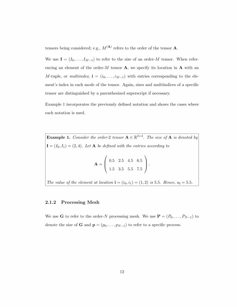
Example 1 incorporates the previously defined notation and shows the cases where

each notation is used.

Example 1. Consider the order-2 tensor A ∈ R2×4. The size of A is denoted by

I = (I0, I1) = (2, 4). Let A be defined with the entries according to

A =

0.5 2.5 4.5 6.5

1.5 3.5 5.5 7.5

.

The value of the element at location i = (i0, i1) = (1, 2) is 5.5. Hence, ai = 5.5.

2.1.2 Processing Mesh

We use G to refer to the order-N processing mesh. We use P = (P0, . . . , PN−1) to

denote the size of G and p = (p0, . . . , pN−1) to refer to a specific process.

12

2.1.3 Ordered Sets

We use capital script letters (A,B, . . .) to refer to sets, and boldface capital script

letters (A,B, . . .) to refer to sets of sets. Ordered sets, or tuples, are sets with an

explicit order of elements. The cardinality of the set A is denoted |A|. We denote

the Cartesian product of the sets A and B as A⊗B. We use braces to denote a set

without order, and parentheses to indicate a set with order. See Example 2.

Example 2. To define the unordered set S containing the elements 4,5, and 7, we

say

S = {4, 5, 7} .

We could equivalently say S = {4, 7, 5}, etc. The cardinality of S is |S| = 3.

To define the ordered set S containing the same elements in, for example, decreas-

ing order, we say

S = (7, 5, 4) .

The ordered set of all valid multiindices is called the range and is denoted by R, as

defined in Definition 1.

13

Definition 1. The set of indices associated with a dimension I ∈ N is denoted

R (I) where

R (I) =

∅ if I = 0

(0, 1, . . . , I − 1) otherwise.

It is convenient to treat this as an ordered set. The set of all multiindices associated

with a size array I = (I0, . . . , IM−1) is denoted R (I) where

R (I) = R (I0)⊗ · · · ⊗ R (IM−1)

and A⊗ B represents the Cartesian product of the sets A and B.

When discussing redistributions and how to derive algorithms, it is useful to view

ordered sets in terms of a prefix and suffix of elements. Definition 2 defines the

concatenation operation on ordered sets; see also Example 3.

Definition 2. The concatenation of two ordered sets is denoted with t; i.e.,

A t B =(a0, . . . , a|A|−1, b0, . . . , b|B|−1

).

Example 3. Consider the ordered sets A = (3, 6, 2) and B = (4, 8). The elements

of C = A t B are

C = (c0, c1, c2, c3, c4) = (a0, a1, a2, b0, b1) = (3, 6, 2, 4, 8) .

14

In order to select or filter entries from an ordered set, we introduce subset selection

in Definition 3.

Definition 3. Given an ordered set S =(s0, . . . , s|S|−1

)and an ordered set

F =(f0, . . . , f|F|−1

)⊆ R (|S|) specifying the entries of S to select, we denote the

tuple with entries of S in the order specified by F as

S (F) =(sf0 , sf1 , . . . , sf|F|−1

).

Example 4. Given an ordered set S = (1, 5, 3, 6,−1) and an ordered set

F = (2, 0, 4) specifying the entries of S to select, then

S (F) = (sf0 , sf1 , sf2) = (s2, s0, s4) = (3, 1,−1) .

2.1.4 Index Conversion

Describing and analyzing tensor distributions requires the mapping from a mul-

tiindex to the corresponding linear index. To give an idea of what this function

represents, consider a matrix whose elements are stored somewhere in memory (lin-

ear array of addresses). In this case, mapping from a multiindex to a linear index

corresponds to taking an element’s location in the matrix and determining its offset

in memory. This function depends on whether the matrix is stored via column- or

row-major order. In this section, we generalize this notion to support the arbitrary

15

mode ordering for storing a higher-order tensor.

Notation for the cumulative product is given in Definition 4.

Definition 4. Given a size array I of an order-M tensor, the function prod (I)

computes the cumulative product, i.e.,

prod (I) =

1 if M = 0∏

`∈R(M)

I` otherwise.

To specify the cumulative product considering only the entries of I at locations

specified by the set S, we say

prod (I,S) = prod (I (S)) .

Definition 5 gives the function to convert multiindices to linear indices.

16

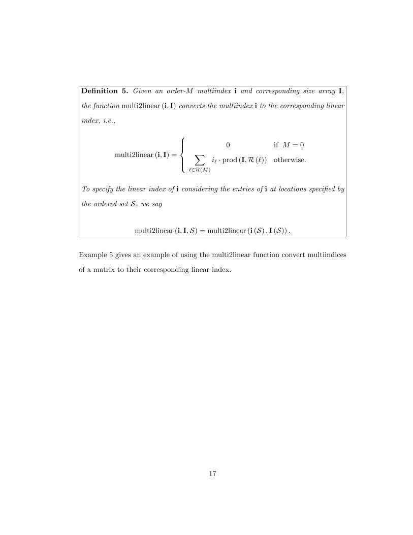
Definition 5. Given an order-M multiindex i and corresponding size array I,

the function multi2linear (i, I) converts the multiindex i to the corresponding linear

index, i.e.,

multi2linear (i, I) =

0 if M = 0∑

`∈R(M)

i` · prod (I,R (`)) otherwise.

To specify the linear index of i considering the entries of i at locations specified by

the ordered set S, we say

multi2linear (i, I,S) = multi2linear (i (S) , I (S)) .

Example 5 gives an example of using the multi2linear function convert multiindices

of a matrix to their corresponding linear index.

17

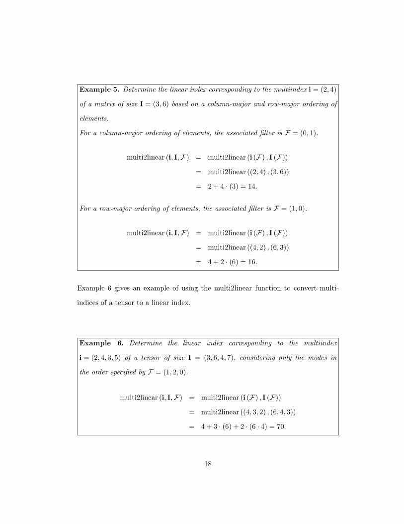
Example 5. Determine the linear index corresponding to the multiindex i = (2, 4)

of a matrix of size I = (3, 6) based on a column-major and row-major ordering of

elements.

For a column-major ordering of elements, the associated filter is F = (0, 1).

multi2linear (i, I,F) = multi2linear (i (F) , I (F))

= multi2linear ((2, 4) , (3, 6))

= 2 + 4 · (3) = 14.

For a row-major ordering of elements, the associated filter is F = (1, 0).

multi2linear (i, I,F) = multi2linear (i (F) , I (F))

= multi2linear ((4, 2) , (6, 3))

= 4 + 2 · (6) = 16.

Example 6 gives an example of using the multi2linear function to convert multi-

indices of a tensor to a linear index.

Example 6. Determine the linear index corresponding to the multiindex

i = (2, 4, 3, 5) of a tensor of size I = (3, 6, 4, 7), considering only the modes in

the order specified by F = (1, 2, 0).

multi2linear (i, I,F) = multi2linear (i (F) , I (F))

= multi2linear ((4, 3, 2) , (6, 4, 3))

= 4 + 3 · (6) + 2 · (6 · 4) = 70.

18

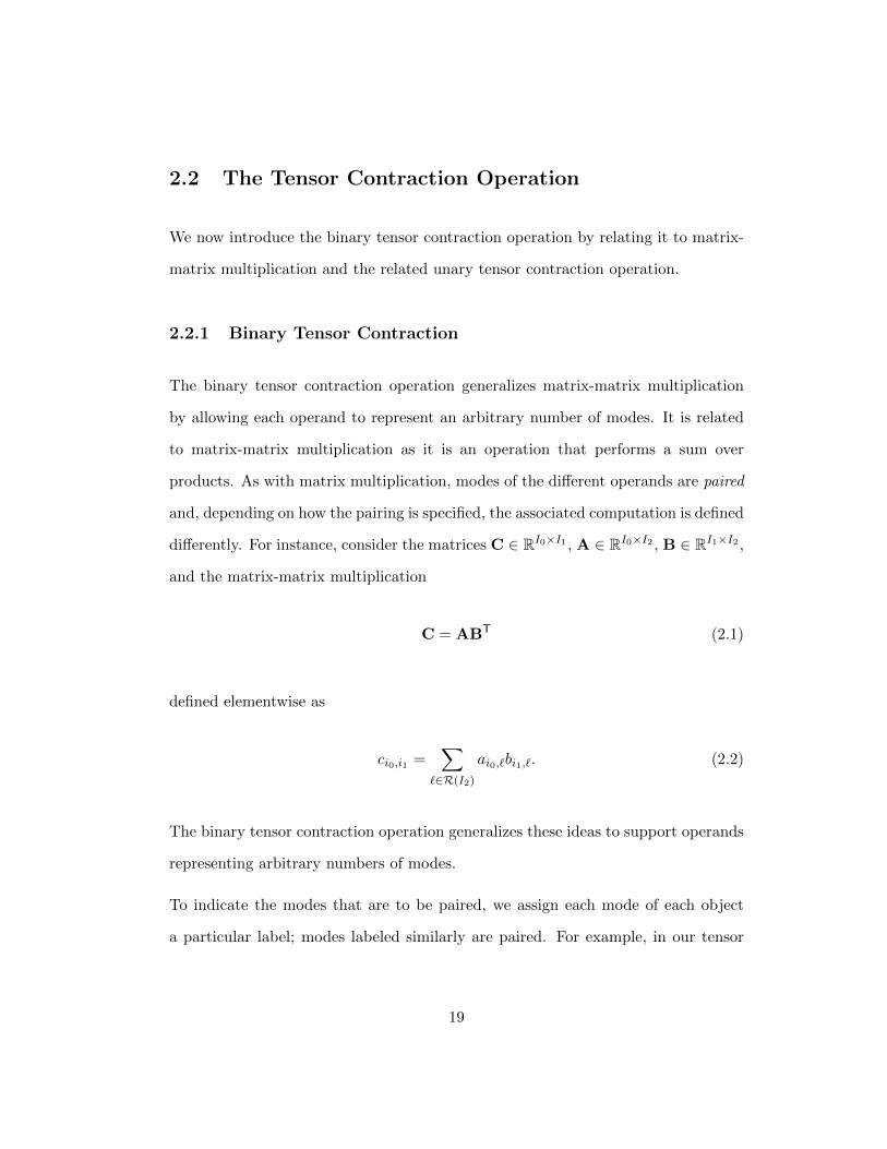
2.2 The Tensor Contraction Operation

We now introduce the binary tensor contraction operation by relating it to matrix-

matrix multiplication and the related unary tensor contraction operation.

2.2.1 Binary Tensor Contraction

The binary tensor contraction operation generalizes matrix-matrix multiplication

by allowing each operand to represent an arbitrary number of modes. It is related

to matrix-matrix multiplication as it is an operation that performs a sum over

products. As with matrix multiplication, modes of the different operands are paired

and, depending on how the pairing is specified, the associated computation is defined

differently. For instance, consider the matrices C ∈ RI0×I1 , A ∈ RI0×I2 , B ∈ RI1×I2 ,

and the matrix-matrix multiplication

C = ABT (2.1)

defined elementwise as

ci0,i1 =∑

`∈R(I2)

ai0,`bi1,`. (2.2)

The binary tensor contraction operation generalizes these ideas to support operands

representing arbitrary numbers of modes.

To indicate the modes that are to be paired, we assign each mode of each object

a particular label; modes labeled similarly are paired. For example, in our tensor

19

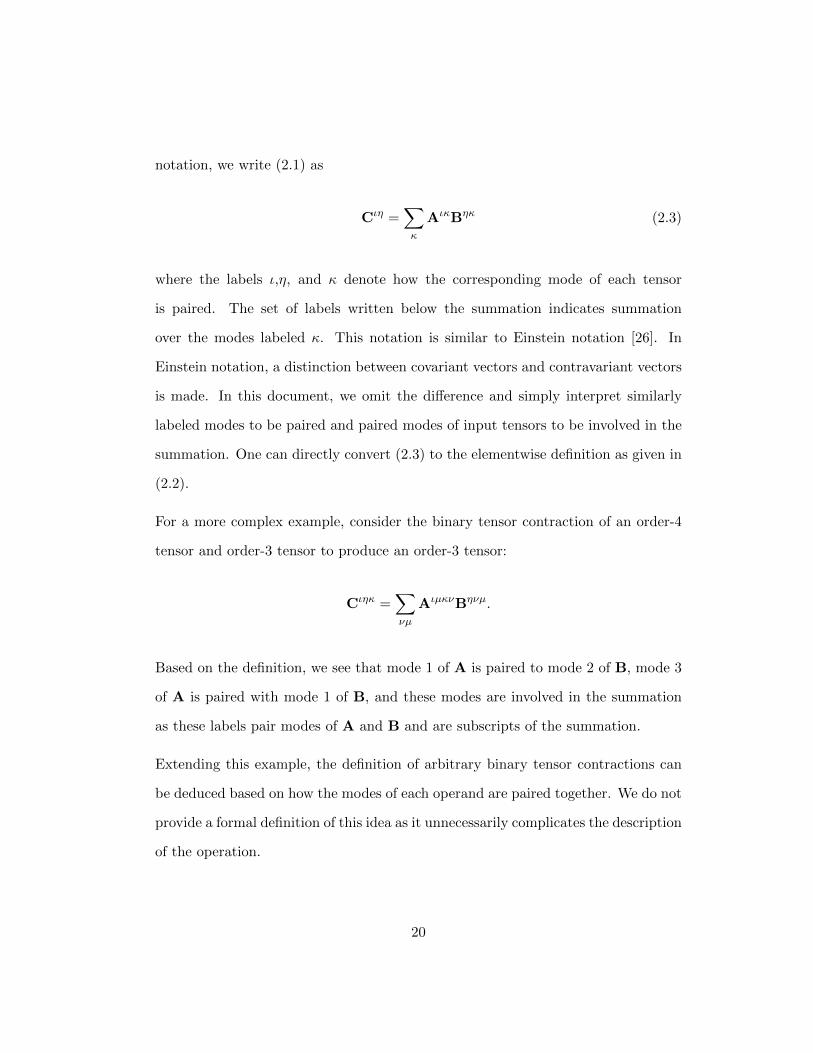
notation, we write (2.1) as

Cιη =∑κ

AικBηκ (2.3)

where the labels ι,η, and κ denote how the corresponding mode of each tensor

is paired. The set of labels written below the summation indicates summation

over the modes labeled κ. This notation is similar to Einstein notation [26]. In

Einstein notation, a distinction between covariant vectors and contravariant vectors

is made. In this document, we omit the difference and simply interpret similarly

labeled modes to be paired and paired modes of input tensors to be involved in the

summation. One can directly convert (2.3) to the elementwise definition as given in

(2.2).

For a more complex example, consider the binary tensor contraction of an order-4

tensor and order-3 tensor to produce an order-3 tensor:

Cιηκ =∑νµ

AιµκνBηνµ.

Based on the definition, we see that mode 1 of A is paired to mode 2 of B, mode 3

of A is paired with mode 1 of B, and these modes are involved in the summation

as these labels pair modes of A and B and are subscripts of the summation.

Extending this example, the definition of arbitrary binary tensor contractions can

be deduced based on how the modes of each operand are paired together. We do not

provide a formal definition of this idea as it unnecessarily complicates the description

of the operation.

20

2.2.2 Unary Tensor Contractions

As the unary tensor contraction only has one input operand, no multiplication

between operands can occur; however, the interpretation of how to accumulate con-

tributions remains the same as in the binary tensor contraction. This operation is

related to the matrix operation which accumulates columns (or rows) of the matrix

together. For instance, consider the unary tensor contraction defined as

Cι =∑η

Aιη.

Based on the definition, we see that we are accumulating entries within mode 1 of

A together. This creates a vector (one-mode) tensor C such that the element ci0 is

the sum of the corresponding row of A.

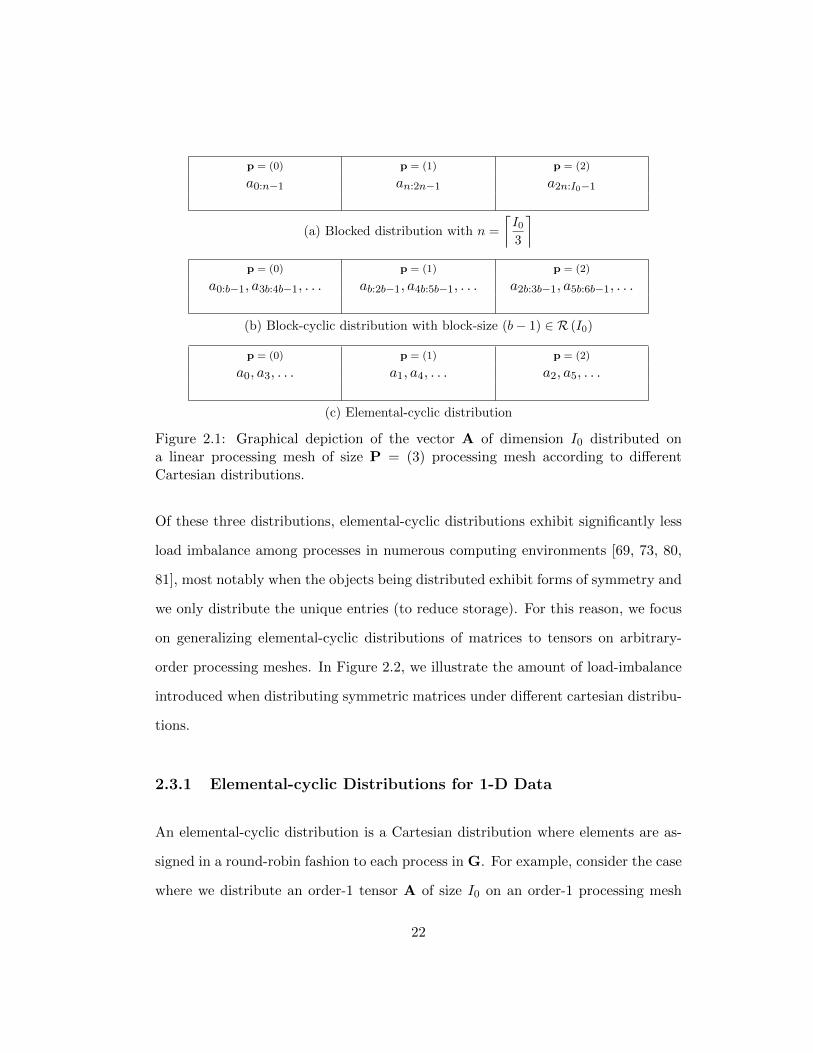
2.3 Data Distributions

In the context of high-performance distributed-memory dense linear algebra, Carte-

sian distributions have commonly been used in high-performance libraries [18, 65,

65, 70, 81, 86]. Examples of Cartesian distributions include blocked, where each

process is assigned a contiguous block of indices; block-cyclic, where each process

is assigned blocks of indices in a round-robin fashion; and elemental-cyclic, where

each process is assigned indices in a round-robin fashion. Illustrations of blocked,

block-cyclic, and elemental-cyclic distributions are given in Figure 2.1. Notice that

an elemental-cyclic distribution (Figure 2.2c) is equivalent to a block-cyclic distri-

bution (Figure 2.2b) with block-size b = 1.

21

p = (0) p = (1) p = (2)

a0:n−1 an:2n−1 a2n:I0−1

(a) Blocked distribution with n =

⌈I03

⌉p = (0) p = (1) p = (2)

a0:b−1, a3b:4b−1, . . . ab:2b−1, a4b:5b−1, . . . a2b:3b−1, a5b:6b−1, . . .

(b) Block-cyclic distribution with block-size (b− 1) ∈ R (I0)

p = (0) p = (1) p = (2)

a0, a3, . . . a1, a4, . . . a2, a5, . . .

(c) Elemental-cyclic distribution

Figure 2.1: Graphical depiction of the vector A of dimension I0 distributed ona linear processing mesh of size P = (3) processing mesh according to differentCartesian distributions.

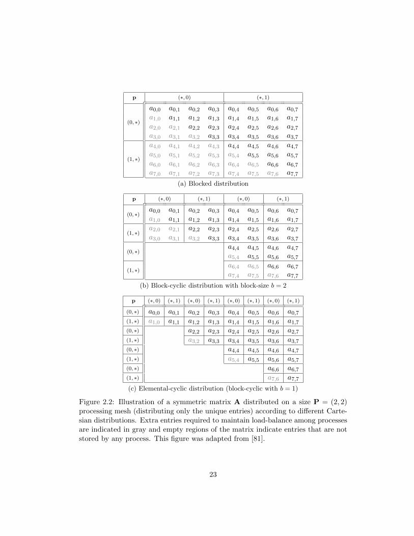
Of these three distributions, elemental-cyclic distributions exhibit significantly less

load imbalance among processes in numerous computing environments [69, 73, 80,

81], most notably when the objects being distributed exhibit forms of symmetry and

we only distribute the unique entries (to reduce storage). For this reason, we focus

on generalizing elemental-cyclic distributions of matrices to tensors on arbitrary-

order processing meshes. In Figure 2.2, we illustrate the amount of load-imbalance

introduced when distributing symmetric matrices under different cartesian distribu-

tions.

2.3.1 Elemental-cyclic Distributions for 1-D Data

An elemental-cyclic distribution is a Cartesian distribution where elements are as-

signed in a round-robin fashion to each process in G. For example, consider the case

where we distribute an order-1 tensor A of size I0 on an order-1 processing mesh

22

p (∗, 0) (∗, 1)

(0, ∗)

a0,0 a0,1 a0,2 a0,3 a0,4 a0,5 a0,6 a0,7a1,0 a1,1 a1,2 a1,3 a1,4 a1,5 a1,6 a1,7a2,0 a2,1 a2,2 a2,3 a2,4 a2,5 a2,6 a2,7a3,0 a3,1 a3,2 a3,3 a3,4 a3,5 a3,6 a3,7

(1, ∗)

a4,0 a4,1 a4,2 a4,3 a4,4 a4,5 a4,6 a4,7a5,0 a5,1 a5,2 a5,3 a5,4 a5,5 a5,6 a5,7a6,0 a6,1 a6,2 a6,3 a6,4 a6,5 a6,6 a6,7a7,0 a7,1 a7,2 a7,3 a7,4 a7,5 a7,6 a7,7

(a) Blocked distribution

p (∗, 0) (∗, 1) (∗, 0) (∗, 1)

(0, ∗)a0,0 a0,1 a0,2 a0,3 a0,4 a0,5 a0,6 a0,7a1,0 a1,1 a1,2 a1,3 a1,4 a1,5 a1,6 a1,7

(1, ∗)a2,0 a2,1 a2,2 a2,3 a2,4 a2,5 a2,6 a2,7a3,0 a3,1 a3,2 a3,3 a3,4 a3,5 a3,6 a3,7

(0, ∗)a4,4 a4,5 a4,6 a4,7a5,4 a5,5 a5,6 a5,7

(1, ∗)a6,4 a6,5 a6,6 a6,7a7,4 a7,5 a7,6 a7,7

(b) Block-cyclic distribution with block-size b = 2

p (∗, 0) (∗, 1) (∗, 0) (∗, 1) (∗, 0) (∗, 1) (∗, 0) (∗, 1)

(0, ∗) a0,0 a0,1 a0,2 a0,3 a0,4 a0,5 a0,6 a0,7(1, ∗) a1,0 a1,1 a1,2 a1,3 a1,4 a1,5 a1,6 a1,7(0, ∗) a2,2 a2,3 a2,4 a2,5 a2,6 a2,7(1, ∗) a3,2 a3,3 a3,4 a3,5 a3,6 a3,7(0, ∗) a4,4 a4,5 a4,6 a4,7(1, ∗) a5,4 a5,5 a5,6 a5,7(0, ∗) a6,6 a6,7(1, ∗) a7,6 a7,7

(c) Elemental-cyclic distribution (block-cyclic with b = 1)

Figure 2.2: Illustration of a symmetric matrix A distributed on a size P = (2, 2)processing mesh (distributing only the unique entries) according to different Carte-sian distributions. Extra entries required to maintain load-balance among processesare indicated in gray and empty regions of the matrix indicate entries that are notstored by any process. This figure was adapted from [81].

23

Assigned rank Assigned indices

0 {0, P0, 2P0, . . .}1 {1, 1 + P0, 1 + 2P0, . . .}...

...

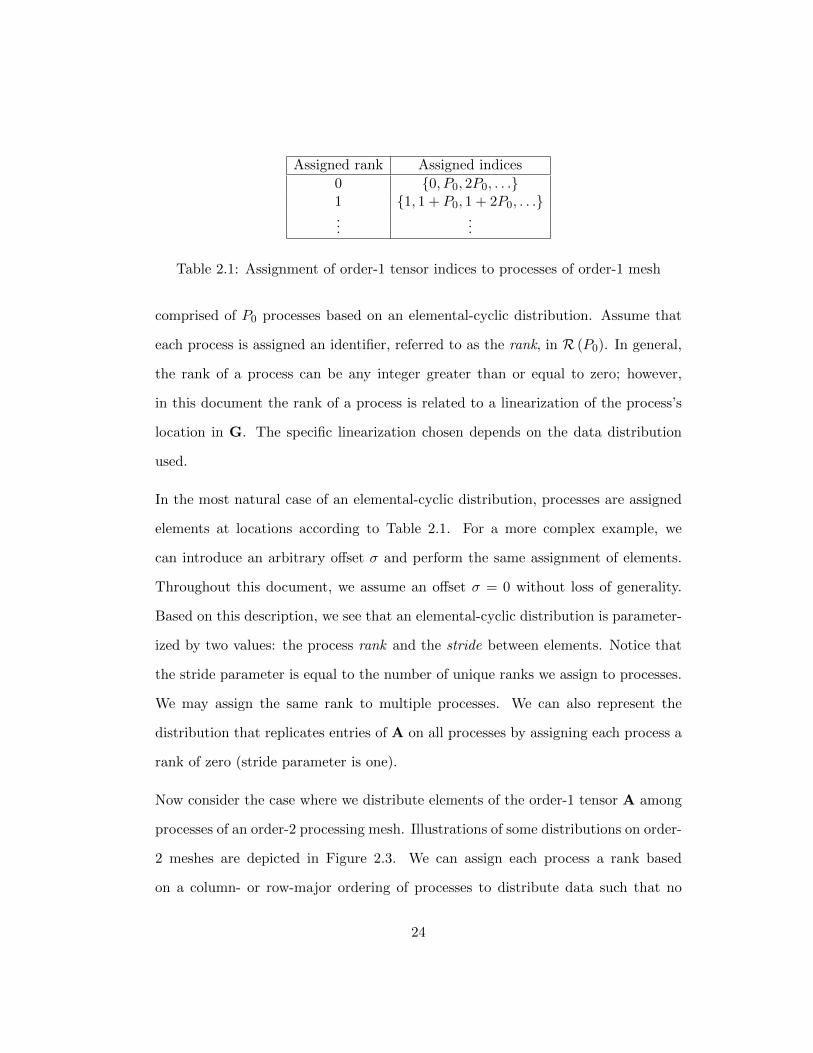
Table 2.1: Assignment of order-1 tensor indices to processes of order-1 mesh

comprised of P0 processes based on an elemental-cyclic distribution. Assume that

each process is assigned an identifier, referred to as the rank, in R (P0). In general,

the rank of a process can be any integer greater than or equal to zero; however,

in this document the rank of a process is related to a linearization of the process’s

location in G. The specific linearization chosen depends on the data distribution

used.

In the most natural case of an elemental-cyclic distribution, processes are assigned

elements at locations according to Table 2.1. For a more complex example, we

can introduce an arbitrary offset σ and perform the same assignment of elements.

Throughout this document, we assume an offset σ = 0 without loss of generality.

Based on this description, we see that an elemental-cyclic distribution is parameter-

ized by two values: the process rank and the stride between elements. Notice that

the stride parameter is equal to the number of unique ranks we assign to processes.

We may assign the same rank to multiple processes. We can also represent the

distribution that replicates entries of A on all processes by assigning each process a

rank of zero (stride parameter is one).

Now consider the case where we distribute elements of the order-1 tensor A among

processes of an order-2 processing mesh. Illustrations of some distributions on order-

2 meshes are depicted in Figure 2.3. We can assign each process a rank based

on a column- or row-major ordering of processes to distribute data such that no

24

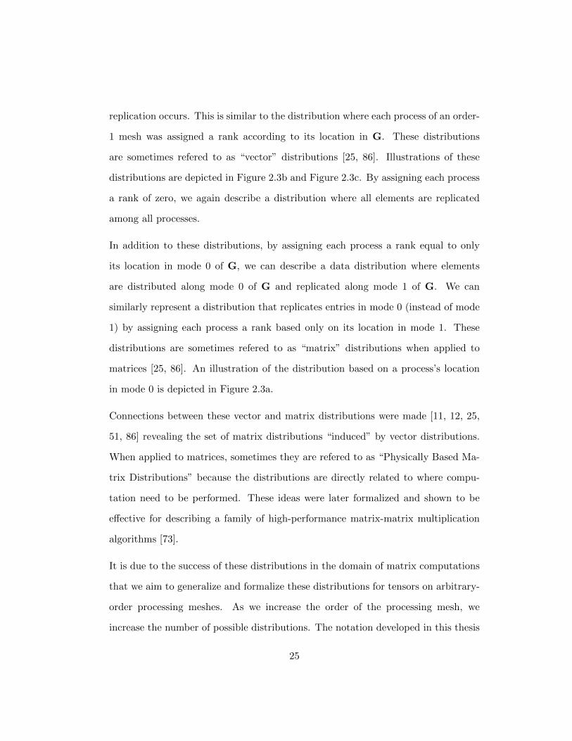
replication occurs. This is similar to the distribution where each process of an order-

1 mesh was assigned a rank according to its location in G. These distributions

are sometimes refered to as “vector” distributions [25, 86]. Illustrations of these

distributions are depicted in Figure 2.3b and Figure 2.3c. By assigning each process

a rank of zero, we again describe a distribution where all elements are replicated

among all processes.

In addition to these distributions, by assigning each process a rank equal to only

its location in mode 0 of G, we can describe a data distribution where elements

are distributed along mode 0 of G and replicated along mode 1 of G. We can

similarly represent a distribution that replicates entries in mode 0 (instead of mode

1) by assigning each process a rank based only on its location in mode 1. These

distributions are sometimes refered to as “matrix” distributions when applied to

matrices [25, 86]. An illustration of the distribution based on a process’s location

in mode 0 is depicted in Figure 2.3a.

Connections between these vector and matrix distributions were made [11, 12, 25,

51, 86] revealing the set of matrix distributions “induced” by vector distributions.

When applied to matrices, sometimes they are refered to as “Physically Based Ma-

trix Distributions” because the distributions are directly related to where compu-

tation need to be performed. These ideas were later formalized and shown to be

effective for describing a family of high-performance matrix-matrix multiplication

algorithms [73].

It is due to the success of these distributions in the domain of matrix computations

that we aim to generalize and formalize these distributions for tensors on arbitrary-

order processing meshes. As we increase the order of the processing mesh, we

increase the number of possible distributions. The notation developed in this thesis

25

p = (0, 0) r = 0 p = (0, 1) r = 0 p = (0, 2) r = 0

a0, a2, . . . a0, a2, . . . a0, a2, . . .

p = (1, 0) r = 1 p = (1, 1) r = 1 p = (1, 2) r = 1

a1, a3, . . . a1, a3, . . . a1, a3, . . .

(a) Mode-0 ordering (stride of two)

p = (0, 0) r = 0 p = (0, 1) r = 2 p = (0, 2) r = 4

a0, a6, . . . a2, a8, . . . a4, a10, . . .

p = (1, 0) r = 1 p = (1, 1) r = 3 p = (1, 2) r = 5

a1, a7, . . . a3, a9, . . . a5, a11, . . .

(b) Mode-(0,1) (column-major) ordering (stride of six)

p = (0, 0) r = 0 p = (0, 1) r = 1 p = (0, 2) r = 2

a0, a6, . . . a1, a7, . . . a2, a8, . . .

p = (1, 0) r = 3 p = (1, 1) r = 4 p = (1, 2) r = 5

a3, a9, . . . a4, a10, . . . a5, a11, . . .

(c) Mode-(1,0) (row-major) ordering (stride of six)

Figure 2.3: Illustration of the vector A distributed in an elemental-cyclic fashion ona processing mesh of size P = (2, 3). The rank of each process is denoted by r.

26

is based on this idea of representing distributions in terms of the ordered set of

modes used to assign ranks to processes. We formalize these ideas in the following

subsections.

2.3.2 Tensor Mode and Tensor Distributions

To define elemental-cyclic distributions for data of an order-M tensor A, we need

to specify the set of multiindices assigned to each process. We do this by assigning

an elemental-cyclic distribution to each mode of the tensor; in other words, we

separately distribute the indices of each tensor mode. We refer to the distribution

of indices of a single mode as a tensor mode distribution and recognize that it is

nothing more than a reinterpretation of elemental-cyclic distributions on order-1

processing meshes.

The combination of the indices in each mode specifies the multiindices of elements

assigned to each process. We refer to the multiindices assigned to each process

as a tensor distribution. We define both tensor mode and tensor distributions in

Definition 6 and provide an example of a tensor distribution in Example 7.

27

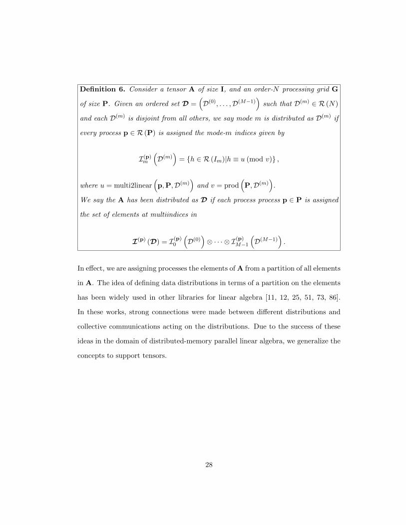
Definition 6. Consider a tensor A of size I, and an order-N processing grid G

of size P. Given an ordered set D =(D(0), . . . ,D(M−1)

)such that D(m) ∈ R (N)

and each D(m) is disjoint from all others, we say mode m is distributed as D(m) if

every process p ∈ R (P) is assigned the mode-m indices given by

I(p)m

(D(m)

)= {h ∈ R (Im)|h ≡ u (mod v)} ,

where u = multi2linear(p,P,D(m)

)and v = prod

(P,D(m)

).

We say the A has been distributed as D if each process process p ∈ P is assigned

the set of elements at multiindices in

I(p) (D) = I(p)0

(D(0)

)⊗ · · · ⊗ I(p)M−1

(D(M−1)

).

In effect, we are assigning processes the elements of A from a partition of all elements

in A. The idea of defining data distributions in terms of a partition on the elements

has been widely used in other libraries for linear algebra [11, 12, 25, 51, 73, 86].

In these works, strong connections were made between different distributions and

collective communications acting on the distributions. Due to the success of these

ideas in the domain of distributed-memory parallel linear algebra, we generalize the

concepts to support tensors.

28

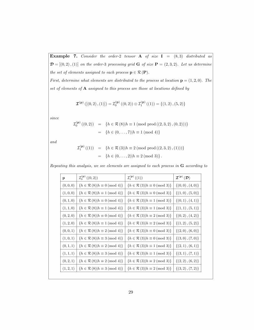
Example 7. Consider the order-2 tensor A of size I = (8, 3) distributed as

D = [(0, 2) , (1)] on the order-3 processing grid G of size P = (2, 3, 2). Let us determine

the set of elements assigned to each process p ∈ R (P).

First, determine what elements are distributed to the process at location p = (1, 2, 0). The

set of elements of A assigned to this process are those at locations defined by

I(p) ([(0, 2) , (1)]) = I(p)0 ((0, 2))⊗ I(p)1 ((1)) = {(1, 2) , (5, 2)}

since

I(p)0 ((0, 2)) = {h ∈ R (8)|h ≡ 1 (mod prod ((2, 3, 2) , (0, 2)))}

= {h ∈ (0, . . . , 7)|h ≡ 1 (mod 4)}

and

I(p)1 ((1)) = {h ∈ R (3)|h ≡ 2 (mod prod ((2, 3, 2) , (1)))}

= {h ∈ (0, . . . , 2)|h ≡ 2 (mod 3)} .

Repeating this analysis, we see elements are assigned to each process in G according to

p I(p)0 ((0, 2)) I(p)

1 ((1)) I(p) (D)

(0, 0, 0) {h ∈ R (8)|h ≡ 0 (mod 4)} {h ∈ R (3)|h ≡ 0 (mod 3)} {(0, 0) , (4, 0)}

(1, 0, 0) {h ∈ R (8)|h ≡ 1 (mod 4)} {h ∈ R (3)|h ≡ 0 (mod 3)} {(1, 0) , (5, 0)}

(0, 1, 0) {h ∈ R (8)|h ≡ 0 (mod 4)} {h ∈ R (3)|h ≡ 1 (mod 3)} {(0, 1) , (4, 1)}

(1, 1, 0) {h ∈ R (8)|h ≡ 1 (mod 4)} {h ∈ R (3)|h ≡ 1 (mod 3)} {(1, 1) , (5, 1)}

(0, 2, 0) {h ∈ R (8)|h ≡ 0 (mod 4)} {h ∈ R (3)|h ≡ 2 (mod 3)} {(0, 2) , (4, 2)}

(1, 2, 0) {h ∈ R (8)|h ≡ 1 (mod 4)} {h ∈ R (3)|h ≡ 2 (mod 3)} {(1, 2) , (5, 2)}

(0, 0, 1) {h ∈ R (8)|h ≡ 2 (mod 4)} {h ∈ R (3)|h ≡ 0 (mod 3)} {(2, 0) , (6, 0)}

(1, 0, 1) {h ∈ R (8)|h ≡ 3 (mod 4)} {h ∈ R (3)|h ≡ 0 (mod 3)} {(3, 0) , (7, 0)}

(0, 1, 1) {h ∈ R (8)|h ≡ 2 (mod 4)} {h ∈ R (3)|h ≡ 1 (mod 3)} {(2, 1) , (6, 1)}

(1, 1, 1) {h ∈ R (8)|h ≡ 3 (mod 4)} {h ∈ R (3)|h ≡ 1 (mod 3)} {(3, 1) , (7, 1)}

(0, 2, 1) {h ∈ R (8)|h ≡ 2 (mod 4)} {h ∈ R (3)|h ≡ 2 (mod 3)} {(2, 2) , (6, 2)}

(1, 2, 1) {h ∈ R (8)|h ≡ 3 (mod 4)} {h ∈ R (3)|h ≡ 2 (mod 3)} {(3, 2) , (7, 2)}

29

Throughout this document we denote the tensor distribution with boldface cap-

ital script D. As a shorthand, to represent the tensor A distributed as D =(D(0), . . . ,D(M−1)

), we write A [D] or A

[D(0), . . . ,D(M−1)

](square brackets used

only for clarity).

Observe that if a tensor mode distribution is empty, then each process is assigned

the full range of tensor mode indices (by definition of multi2linear and prod). Also

notice that data is replicated over all processing mesh modes that are not used in

the tensor distribution. In other words, data is replicated over mode n of G if

n 6∈⋃

m∈R(M)

D(m).

2.3.3 Advanced Tensor Distributions

At this point we have defined a set of tensor distributions that assign elements of

A to each process in G. Under the current interpretation of tensor distributions, if

a processing mesh mode is excluded from the tensor distribution, the elements of A

are replicated among processes within this excluded mode of G. However, as we see

later on, in certain situations it is useful to be able to represent cases where the data

of A is assigned to only one process in this excluded mode of G (all other processes

assigned no data). These distributions arise as the result of “-to-one” collectives

such as gather-to-one and reduce-to-one.

For example, consider the case where G is of size P = (3, 4, 2) and we desire to

distribute A according to A [(0) , (1)] but only assign elements to those processes

whose location in mode 2 is zero.

To support these kinds of distributions, we augment our notation with the set of

30

modes over which we should not implicitly replicate1. The notation used for these

distributions is defined in Definition 7.

Definition 7. Consider the order-M tensor A of size I to be distributed over

processes of the order-N processing mesh G of size P according to the tensor dis-

tribution D =(D(0), . . . ,D(M−1)

). Let E be the set of modes over which replication

should not implicitly occur and let w ∈ R (prod (P, E)).

We say A has been distributed as A [D; E , w] if all processes in p ∈ R (P) are

assigned elements of A according to

I(p) (D; E , w) =

I(p) (D) if multi2linear (p,P, E) = w

∅ otherwise.

We interprete the omission of E and w from I(p) (D; E , w) to indicate E = ∅ and

w = 0.

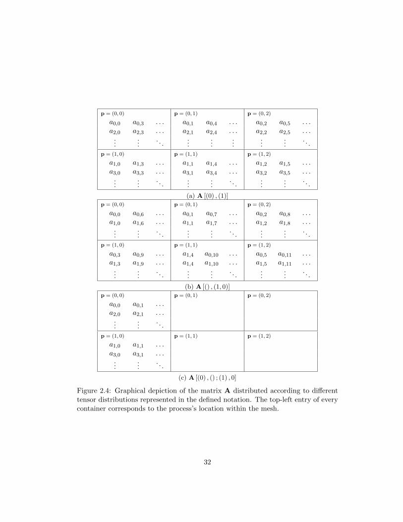
For conciseness, replication over modes omitted from tensor distribution is assumed

unless explicitly stated with the notation introduced in this subsection. In Fig-

ure 2.4, we show examples of different tensor distributions for matrices distributed

on a rectangular processing mesh.

1It may seem more natural to explicitly state the modes over which replication occurs, howeverfor historical reasons we choose to indicate the modes over which replication does not occur.

31

p = (0, 0) p = (0, 1) p = (0, 2)

a0,0 a0,3 . . . a0,1 a0,4 . . . a0,2 a0,5 . . .a2,0 a2,3 . . . a2,1 a2,4 . . . a2,2 a2,5 . . ....

.... . .

......

......

.... . .

p = (1, 0) p = (1, 1) p = (1, 2)

a1,0 a1,3 . . . a1,1 a1,4 . . . a1,2 a1,5 . . .a3,0 a3,3 . . . a3,1 a3,4 . . . a3,2 a3,5 . . ....

.... . .

......

. . ....

.... . .

(a) A [(0) , (1)]

p = (0, 0) p = (0, 1) p = (0, 2)

a0,0 a0,6 . . . a0,1 a0,7 . . . a0,2 a0,8 . . .a1,0 a1,6 . . . a1,1 a1,7 . . . a1,2 a1,8 . . ....

.... . .

......

. . ....

.... . .

p = (1, 0) p = (1, 1) p = (1, 2)

a0,3 a0,9 . . . a1,4 a0,10 . . . a0,5 a0,11 . . .a1,3 a1,9 . . . a1,4 a1,10 . . . a1,5 a1,11 . . ....

.... . .

......

. . ....

.... . .

(b) A [() , (1, 0)]

p = (0, 0) p = (0, 1) p = (0, 2)

a0,0 a0,1 . . .a2,0 a2,1 . . ....

.... . .

p = (1, 0) p = (1, 1) p = (1, 2)

a1,0 a1,1 . . .a3,0 a3,1 . . ....

.... . .

(c) A [(0) , () ; (1) , 0]

Figure 2.4: Graphical depiction of the matrix A distributed according to differenttensor distributions represented in the defined notation. The top-left entry of everycontainer corresponds to the process’s location within the mesh.

32

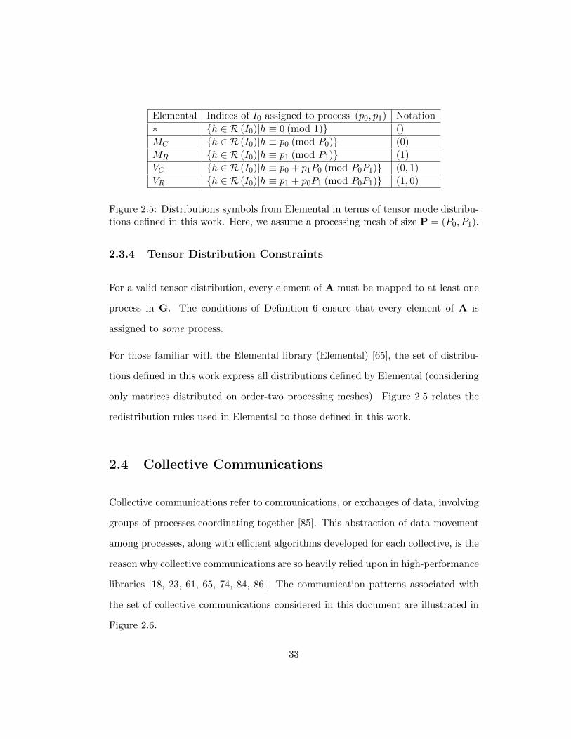
Elemental Indices of I0 assigned to process (p0, p1) Notation

∗ {h ∈ R (I0)|h ≡ 0 (mod 1)} ()

MC {h ∈ R (I0)|h ≡ p0 (mod P0)} (0)

MR {h ∈ R (I0)|h ≡ p1 (mod P1)} (1)

VC {h ∈ R (I0)|h ≡ p0 + p1P0 (mod P0P1)} (0, 1)

VR {h ∈ R (I0)|h ≡ p1 + p0P1 (mod P0P1)} (1, 0)

Figure 2.5: Distributions symbols from Elemental in terms of tensor mode distribu-tions defined in this work. Here, we assume a processing mesh of size P = (P0, P1).

2.3.4 Tensor Distribution Constraints

For a valid tensor distribution, every element of A must be mapped to at least one

process in G. The conditions of Definition 6 ensure that every element of A is

assigned to some process.

For those familiar with the Elemental library (Elemental) [65], the set of distribu-

tions defined in this work express all distributions defined by Elemental (considering

only matrices distributed on order-two processing meshes). Figure 2.5 relates the

redistribution rules used in Elemental to those defined in this work.

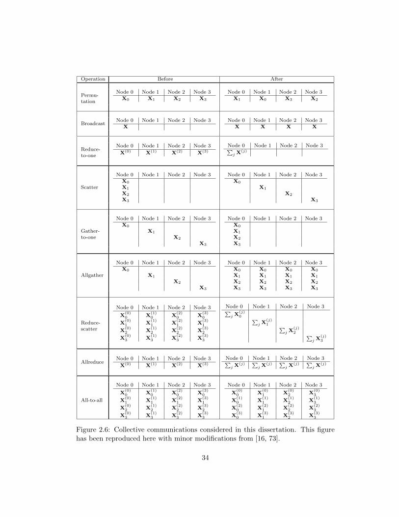
2.4 Collective Communications

Collective communications refer to communications, or exchanges of data, involving

groups of processes coordinating together [85]. This abstraction of data movement

among processes, along with efficient algorithms developed for each collective, is the

reason why collective communications are so heavily relied upon in high-performance

libraries [18, 23, 61, 65, 74, 84, 86]. The communication patterns associated with

the set of collective communications considered in this document are illustrated in

Figure 2.6.

33

Operation Before After

Permu-tation

Node 0 Node 1 Node 2 Node 3X0 X1 X2 X3

Node 0 Node 1 Node 2 Node 3X1 X0 X3 X2

BroadcastNode 0 Node 1 Node 2 Node 3

XNode 0 Node 1 Node 2 Node 3

X X X X

Reduce-to-one

Node 0 Node 1 Node 2 Node 3

X(0) X(1) X(2) X(3)

Node 0 Node 1 Node 2 Node 3∑j X

(j)

Scatter

Node 0 Node 1 Node 2 Node 3X0

X1

X2

X3

Node 0 Node 1 Node 2 Node 3X0

X1

X2

X3

Gather-to-one

Node 0 Node 1 Node 2 Node 3X0

X1

X2

X3

Node 0 Node 1 Node 2 Node 3X0

X1

X2

X3

Allgather

Node 0 Node 1 Node 2 Node 3X0

X1

X2

X3

Node 0 Node 1 Node 2 Node 3X0 X0 X0 X0

X1 X1 X1 X1

X2 X2 X2 X2

X3 X3 X3 X3

Reduce-scatter

Node 0 Node 1 Node 2 Node 3

X(0)0 X

(1)0 X

(2)0 X

(3)0

X(0)1 X

(1)1 X

(2)1 X

(3)1

X(0)2 X

(1)2 X

(2)2 X

(3)2

X(0)3 X

(1)3 X

(2)3 X

(3)3

Node 0 Node 1 Node 2 Node 3∑j X

(j)0 ∑

j X(j)1 ∑

j X(j)2 ∑

j X(j)3

AllreduceNode 0 Node 1 Node 2 Node 3

X(0) X(1) X(2) X(3)

Node 0 Node 1 Node 2 Node 3∑j X

(j) ∑j X

(j) ∑j X

(j) ∑j X

(j)

All-to-all

Node 0 Node 1 Node 2 Node 3

X(0)0 X

(1)0 X

(2)0 X

(3)0

X(0)1 X

(1)1 X

(2)1 X

(3)1

X(0)2 X

(1)2 X

(2)2 X

(3)2

X(0)3 X

(1)3 X

(2)3 X

(3)3

Node 0 Node 1 Node 2 Node 3

X(0)0 X

(0)1 X

(0)2 X

(0)3

X(1)0 X

(1)1 X

(1)2 X

(1)3

X(2)0 X

(2)1 X

(2)2 X

(2)3

X(3)0 X

(3)1 X

(3)2 X

(3)3

Figure 2.6: Collective communications considered in this dissertation. This figurehas been reproduced here with minor modifications from [16, 73].

34

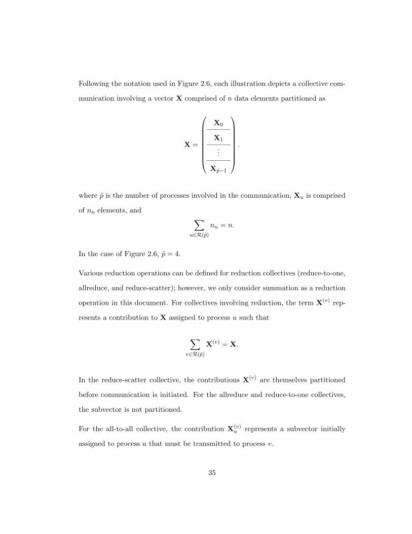
Following the notation used in Figure 2.6, each illustration depicts a collective com-

munication involving a vector X comprised of n data elements partitioned as

X =

X0

X1

...

Xp−1

.

where p is the number of processes involved in the communication, Xu is comprised

of nu elements, and ∑u∈R(p)

nu = n.

In the case of Figure 2.6, p = 4.

Various reduction operations can be defined for reduction collectives (reduce-to-one,

allreduce, and reduce-scatter); however, we only consider summation as a reduction

operation in this document. For collectives involving reduction, the term X(v) rep-

resents a contribution to X assigned to process u such that

∑v∈R(p)

X(v) = X.

In the reduce-scatter collective, the contributions X(v) are themselves partitioned

before communication is initiated. For the allreduce and reduce-to-one collectives,

the subvector is not partitioned.

For the all-to-all collective, the contribution X(v)u represents a subvector initially

assigned to process u that must be transmitted to process v.

35

Each collective then exchanges some combination of the objects associated with

X, the subvectors, Xu, and the contributions, X(v) and X(v)u . For example, if we

look at the pattern for the broadcast collective, we see that initially one process

is assigned the entire vector X. Upon completion, each process involved in the

collective receives the vector X. In the case of the reduce-to-one collective, each

process is assigned a contribution to X and, upon completion, a single process

receives data that represents the summation of all contributions. Finally, if we look

at the scatter collective, initially one process is assigned X and, upon completion,

each process its associated subvector. All other collectives can be interpreted based

on a combination of these examples.

If the size of all subvectors communicated (nu) are approximately equal2, then we

say the associated communication is “balanced”; otherwise, the communication is

“unbalanced”. For an example of an unbalanced communication, consider that a

broadcast collective can be implemented with an all-to-all collective. In this case, one

process is assigned the entire vector X. For this process, the size of the subvector

assigned is n. Consequently, all other processes must be assigned a subvector of

size zero. As the size of each subvector assigned to every process involved in the

collective are not approximately equal, the all-to-all communication (when used in

this context) is unbalanced.

We consider the cost of each collective listed in Figure 2.6 in terms of three pa-

rameters: the time to initiate communication (latency), represented by α; the time

required to transmit data (inverse of bandwidth), represented by β; and the time

to perform an arithmetic computation, represented by γ. For each collective in

2Each process is assigned either

⌊n

p

⌋or

⌊n

p

⌋+ 1 data elements.

36

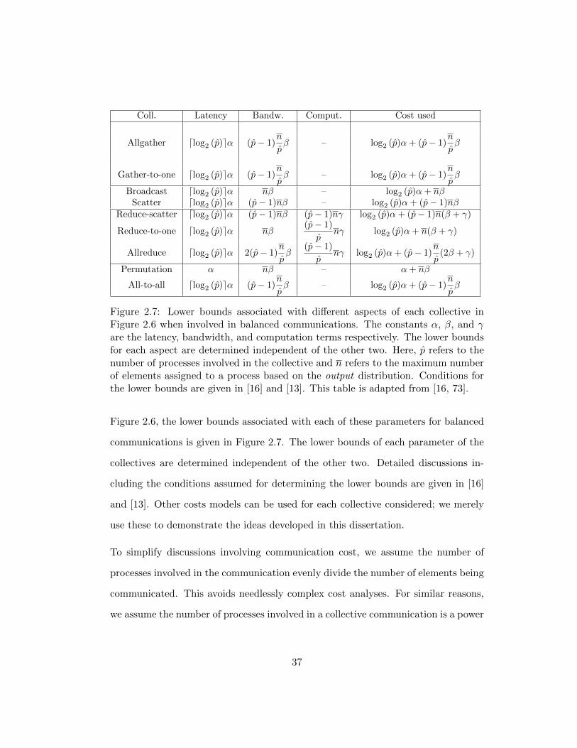
Coll. Latency Bandw. Comput. Cost used

Allgather dlog2 (p)eα (p− 1)n

pβ – log2 (p)α+ (p− 1)

n

pβ

Gather-to-one dlog2 (p)eα (p− 1)n

pβ – log2 (p)α+ (p− 1)

n

pβ

Broadcast dlog2 (p)eα nβ – log2 (p)α+ nβScatter dlog2 (p)eα (p− 1)nβ – log2 (p)α+ (p− 1)nβ

Reduce-scatter dlog2 (p)eα (p− 1)nβ (p− 1)nγ log2 (p)α+ (p− 1)n(β + γ)

Reduce-to-one dlog2 (p)eα nβ(p− 1)

pnγ log2 (p)α+ n(β + γ)

Allreduce dlog2 (p)eα 2(p− 1)n

pβ

(p− 1)

pnγ log2 (p)α+ (p− 1)

n

p(2β + γ)

Permutation α nβ – α+ nβ

All-to-all dlog2 (p)eα (p− 1)n

pβ – log2 (p)α+ (p− 1)

n

pβ

Figure 2.7: Lower bounds associated with different aspects of each collective inFigure 2.6 when involved in balanced communications. The constants α, β, and γare the latency, bandwidth, and computation terms respectively. The lower boundsfor each aspect are determined independent of the other two. Here, p refers to thenumber of processes involved in the collective and n refers to the maximum numberof elements assigned to a process based on the output distribution. Conditions forthe lower bounds are given in [16] and [13]. This table is adapted from [16, 73].

Figure 2.6, the lower bounds associated with each of these parameters for balanced

communications is given in Figure 2.7. The lower bounds of each parameter of the

collectives are determined independent of the other two. Detailed discussions in-

cluding the conditions assumed for determining the lower bounds are given in [16]

and [13]. Other costs models can be used for each collective considered; we merely

use these to demonstrate the ideas developed in this dissertation.

To simplify discussions involving communication cost, we assume the number of

processes involved in the communication evenly divide the number of elements being

communicated. This avoids needlessly complex cost analyses. For similar reasons,

we assume the number of processes involved in a collective communication is a power

37

of two.

We encode only the “balanced” forms of the collectives given in Figure 2.6. How-

ever, some redistributions defined in the notation are inherently unbalanced. In

Chapter 4, we discuss transformations that can be applied to these redistributions,

under certain conditions to perform the equivalent redistribution with balanced

communications. The goal of this process is to reduce the cost associated with

communication.

2.5 Data Redistributions

Our goal in this section is to formalize collective communications in terms of redis-

tributions described by the notation developed in Section 2.3.

We begin with examples from parallel matrix-matrix multiplication that highlight

situations where different collective communications are utilized to create algorithms

with efficient implementations. These examples come from a family, or class, of

algorithms for matrix-matrix multiplication that assume one operand is significantly

larger (in terms of number of elements) than the other two. To reduce the volume

of data communicated, algorithms in this family communicate only data of the

“smaller” operands and data of the “large” operand is not communicated at all.

Algorithms based on this principle are referred to as stationary.

A detailed discussion of each stationary algorithm for matrix-matrix multiplication,

along with the derivation process used to arrive at each algorithm, is given in Morrow

et al. [30] and Schatz et al. [73]. Here, we merely restate the results using our

notation.

38

For each algorithm discussed, an illustration is provided for visual reference (Fig-

ures 2.9, 2.10, 2.11, and 2.12). In each of these figures, we show how each matrix

is distributed during each step of the algorithm and provide the series of collectives

required to perform the associated redistribution. To conserve space, we depict the

distributions of the output object along with any introduced temporaries in the

same location of the illustration.

For the example algorithms discussed, we assume computation is begin performed

on a processing mesh of size P = (P0, P1) and the cost associated with each collective

communication as given in Figure 2.7. Additionally, we assume that integral ratios

exist between dimensions of the distributed object and those of the processing mesh.

This is done only to simplify the discussion of cost analyses.

We use MATLAB-style notation to refer to a column or row of a matrix; i.e., A:,`

refers to the `-th column of the matrix A, and A`,: refers to the `-th row of the matrix

A. We interpret columns and rows of matrices as order-1 objects for consistency in

the developed notation for data distribution.

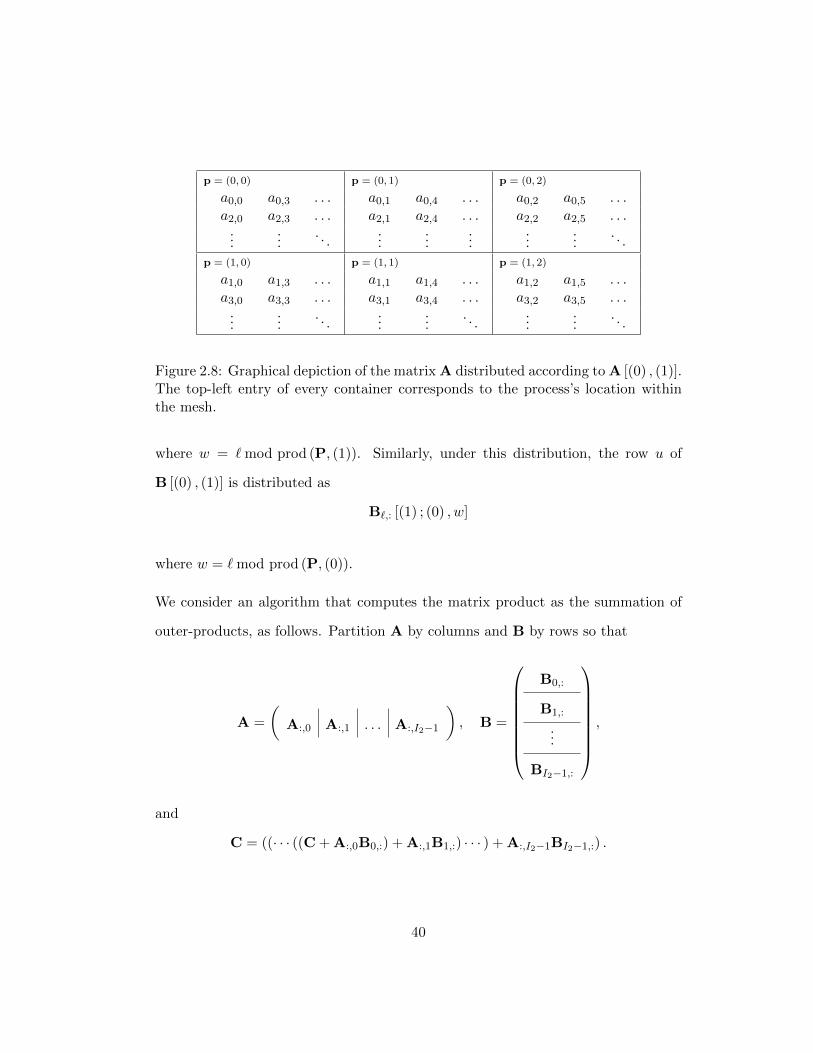
2.5.1 Example: Stationary C Parallel Matrix Multiplication

Consider the operation C = AB + C where C is an I0 × I1 matrix, A is an I0 × I2

matrix, and I2 is small relative to I0 and I1. For purposes of this example, we assume

an initial distribution of A [(0) , (1)], B [(0) , (1)], and C [(0) , (1)]. An illustration of

this initial distribution on a processing mesh of size P = (2, 3) is given in Figure 2.8.

Observe that column u of the matrix A [(0) , (1)] is distributed as

A:,` [(0) ; (1) , w] ,

39

p = (0, 0) p = (0, 1) p = (0, 2)

a0,0 a0,3 . . . a0,1 a0,4 . . . a0,2 a0,5 . . .a2,0 a2,3 . . . a2,1 a2,4 . . . a2,2 a2,5 . . ....

.... . .

......

......

.... . .

p = (1, 0) p = (1, 1) p = (1, 2)

a1,0 a1,3 . . . a1,1 a1,4 . . . a1,2 a1,5 . . .a3,0 a3,3 . . . a3,1 a3,4 . . . a3,2 a3,5 . . ....

.... . .

......

. . ....

.... . .

Figure 2.8: Graphical depiction of the matrix A distributed according to A [(0) , (1)].The top-left entry of every container corresponds to the process’s location withinthe mesh.

where w = `mod prod (P, (1)). Similarly, under this distribution, the row u of

B [(0) , (1)] is distributed as

B`,: [(1) ; (0) , w]

where w = `mod prod (P, (0)).

We consider an algorithm that computes the matrix product as the summation of

outer-products, as follows. Partition A by columns and B by rows so that

A =

(A:,0 A:,1 . . . A:,I2−1

), B =

B0,:

B1,:

...

BI2−1,:

,

and

C = ((· · · ((C + A:,0B0,:) + A:,1B1,:) · · · ) + A:,I2−1BI2−1,:) .

40

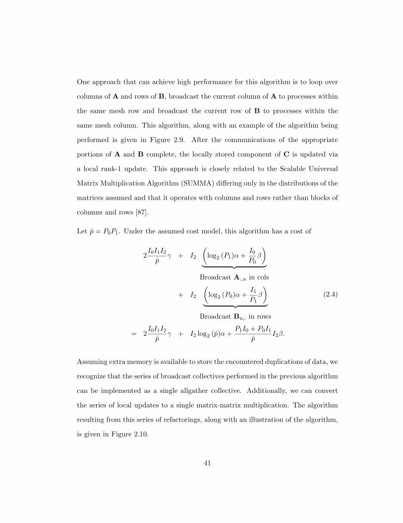
One approach that can achieve high performance for this algorithm is to loop over

columns of A and rows of B, broadcast the current column of A to processes within

the same mesh row and broadcast the current row of B to processes within the

same mesh column. This algorithm, along with an example of the algorithm being

performed is given in Figure 2.9. After the communications of the appropriate

portions of A and B complete, the locally stored component of C is updated via

a local rank-1 update. This approach is closely related to the Scalable Universal

Matrix Multiplication Algorithm (SUMMA) differing only in the distributions of the

matrices assumed and that it operates with columns and rows rather than blocks of

columns and rows [87].

Let p = P0P1. Under the assumed cost model, this algorithm has a cost of

2I0I1I2p

γ + I2

(log2 (P1)α+

I0P0β

)︸ ︷︷ ︸

Broadcast A:,u in cols

+ I2

(log2 (P0)α+

I1P1β

)︸ ︷︷ ︸

Broadcast Bu,: in rows

= 2I0I1I2p

γ + I2 log2 (p)α+P1I0 + P0I1

pI2β.

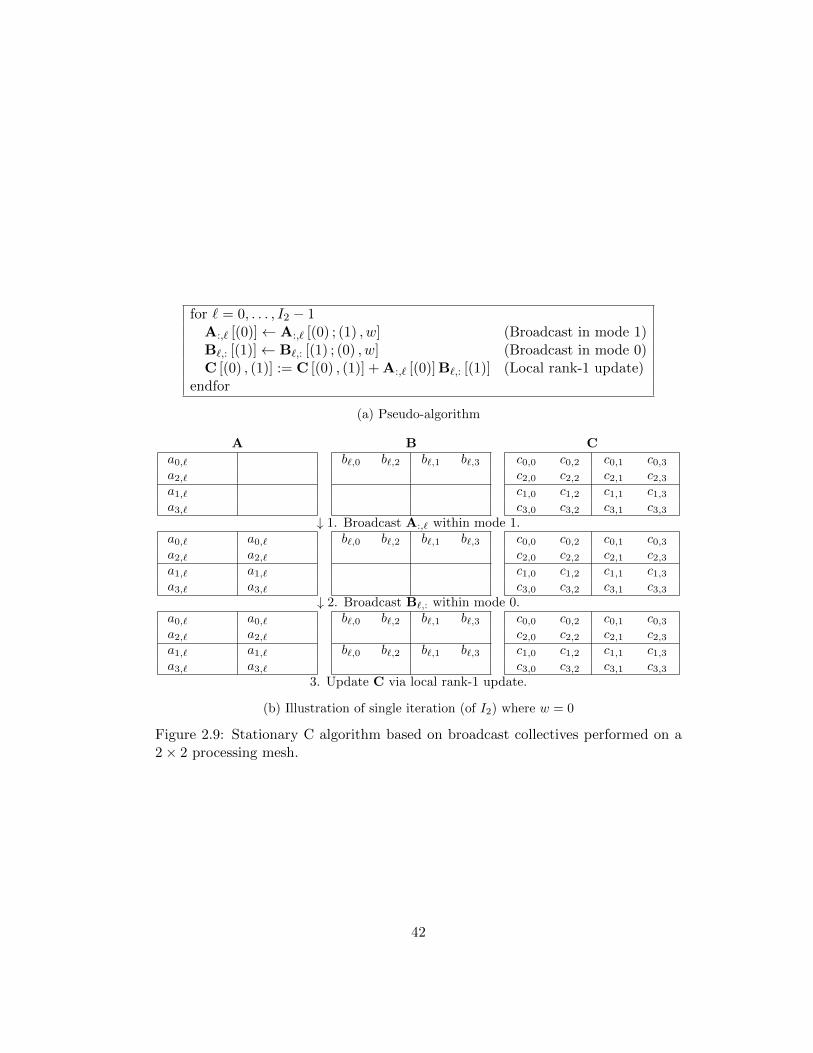
(2.4)

Assuming extra memory is available to store the encountered duplications of data, we

recognize that the series of broadcast collectives performed in the previous algorithm

can be implemented as a single allgather collective. Additionally, we can convert

the series of local updates to a single matrix-matrix multiplication. The algorithm

resulting from this series of refactorings, along with an illustration of the algorithm,

is given in Figure 2.10.

41

for ` = 0, . . . , I2 − 1A:,` [(0)]← A:,` [(0) ; (1) , w] (Broadcast in mode 1)B`,: [(1)]← B`,: [(1) ; (0) , w] (Broadcast in mode 0)C [(0) , (1)] := C [(0) , (1)] + A:,` [(0)] B`,: [(1)] (Local rank-1 update)

endfor

(a) Pseudo-algorithm

A B Ca0,` b`,0 b`,2 b`,1 b`,3 c0,0 c0,2 c0,1 c0,3a2,` c2,0 c2,2 c2,1 c2,3a1,` c1,0 c1,2 c1,1 c1,3a3,` c3,0 c3,2 c3,1 c3,3

↓ 1. Broadcast A:,` within mode 1.a0,` a0,` b`,0 b`,2 b`,1 b`,3 c0,0 c0,2 c0,1 c0,3a2,` a2,` c2,0 c2,2 c2,1 c2,3a1,` a1,` c1,0 c1,2 c1,1 c1,3a3,` a3,` c3,0 c3,2 c3,1 c3,3

↓ 2. Broadcast B`,: within mode 0.a0,` a0,` b`,0 b`,2 b`,1 b`,3 c0,0 c0,2 c0,1 c0,3a2,` a2,` c2,0 c2,2 c2,1 c2,3a1,` a1,` b`,0 b`,2 b`,1 b`,3 c1,0 c1,2 c1,1 c1,3a3,` a3,` c3,0 c3,2 c3,1 c3,3

3. Update C via local rank-1 update.

(b) Illustration of single iteration (of I2) where w = 0

Figure 2.9: Stationary C algorithm based on broadcast collectives performed on a2× 2 processing mesh.

42

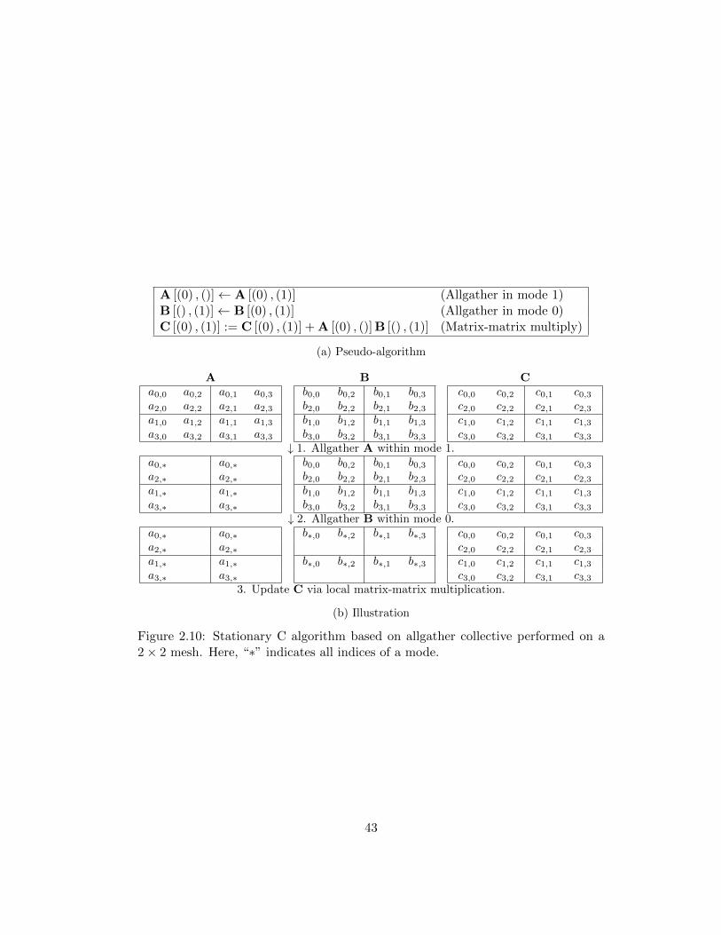
A [(0) , ()]← A [(0) , (1)] (Allgather in mode 1)B [() , (1)]← B [(0) , (1)] (Allgather in mode 0)C [(0) , (1)] := C [(0) , (1)] + A [(0) , ()] B [() , (1)] (Matrix-matrix multiply)

(a) Pseudo-algorithm

A B Ca0,0 a0,2 a0,1 a0,3 b0,0 b0,2 b0,1 b0,3 c0,0 c0,2 c0,1 c0,3a2,0 a2,2 a2,1 a2,3 b2,0 b2,2 b2,1 b2,3 c2,0 c2,2 c2,1 c2,3a1,0 a1,2 a1,1 a1,3 b1,0 b1,2 b1,1 b1,3 c1,0 c1,2 c1,1 c1,3a3,0 a3,2 a3,1 a3,3 b3,0 b3,2 b3,1 b3,3 c3,0 c3,2 c3,1 c3,3

↓ 1. Allgather A within mode 1.a0,∗ a0,∗ b0,0 b0,2 b0,1 b0,3 c0,0 c0,2 c0,1 c0,3a2,∗ a2,∗ b2,0 b2,2 b2,1 b2,3 c2,0 c2,2 c2,1 c2,3a1,∗ a1,∗ b1,0 b1,2 b1,1 b1,3 c1,0 c1,2 c1,1 c1,3a3,∗ a3,∗ b3,0 b3,2 b3,1 b3,3 c3,0 c3,2 c3,1 c3,3

↓ 2. Allgather B within mode 0.a0,∗ a0,∗ b∗,0 b∗,2 b∗,1 b∗,3 c0,0 c0,2 c0,1 c0,3a2,∗ a2,∗ c2,0 c2,2 c2,1 c2,3a1,∗ a1,∗ b∗,0 b∗,2 b∗,1 b∗,3 c1,0 c1,2 c1,1 c1,3a3,∗ a3,∗ c3,0 c3,2 c3,1 c3,3

3. Update C via local matrix-matrix multiplication.

(b) Illustration

Figure 2.10: Stationary C algorithm based on allgather collective performed on a2× 2 mesh. Here, “∗” indicates all indices of a mode.

43

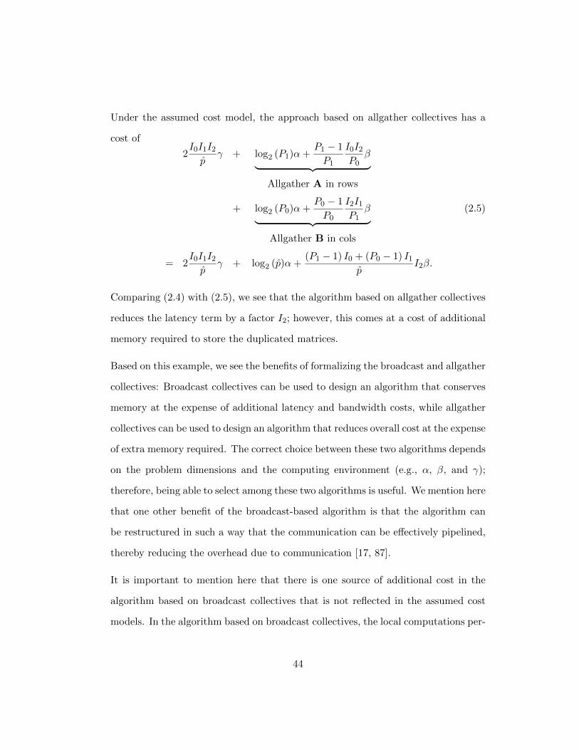
Under the assumed cost model, the approach based on allgather collectives has a

cost of

2I0I1I2p

γ + log2 (P1)α+P1 − 1

P1

I0I2P0

β︸ ︷︷ ︸Allgather A in rows

+ log2 (P0)α+P0 − 1

P0

I2I1P1

β︸ ︷︷ ︸Allgather B in cols

= 2I0I1I2p

γ + log2 (p)α+(P1 − 1) I0 + (P0 − 1) I1

pI2β.

(2.5)

Comparing (2.4) with (2.5), we see that the algorithm based on allgather collectives

reduces the latency term by a factor I2; however, this comes at a cost of additional

memory required to store the duplicated matrices.

Based on this example, we see the benefits of formalizing the broadcast and allgather

collectives: Broadcast collectives can be used to design an algorithm that conserves

memory at the expense of additional latency and bandwidth costs, while allgather

collectives can be used to design an algorithm that reduces overall cost at the expense

of extra memory required. The correct choice between these two algorithms depends

on the problem dimensions and the computing environment (e.g., α, β, and γ);

therefore, being able to select among these two algorithms is useful. We mention here

that one other benefit of the broadcast-based algorithm is that the algorithm can

be restructured in such a way that the communication can be effectively pipelined,

thereby reducing the overhead due to communication [17, 87].

It is important to mention here that there is one source of additional cost in the

algorithm based on broadcast collectives that is not reflected in the assumed cost

models. In the algorithm based on broadcast collectives, the local computations per-

44

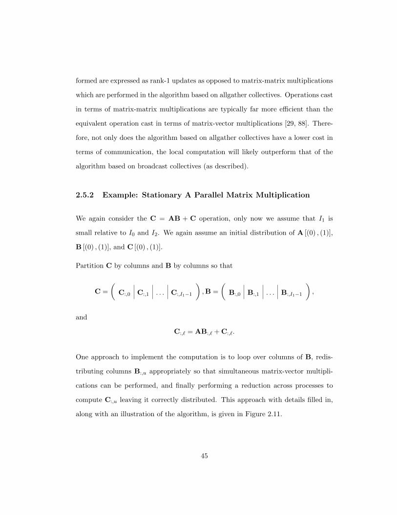
formed are expressed as rank-1 updates as opposed to matrix-matrix multiplications

which are performed in the algorithm based on allgather collectives. Operations cast

in terms of matrix-matrix multiplications are typically far more efficient than the

equivalent operation cast in terms of matrix-vector multiplications [29, 88]. There-

fore, not only does the algorithm based on allgather collectives have a lower cost in

terms of communication, the local computation will likely outperform that of the

algorithm based on broadcast collectives (as described).

2.5.2 Example: Stationary A Parallel Matrix Multiplication

We again consider the C = AB + C operation, only now we assume that I1 is

small relative to I0 and I2. We again assume an initial distribution of A [(0) , (1)],

B [(0) , (1)], and C [(0) , (1)].

Partition C by columns and B by columns so that

C =

(C:,0 C:,1 . . . C:,I1−1

),B =

(B:,0 B:,1 . . . B:,I1−1

),

and

C:,` = AB:,` + C:,`.

One approach to implement the computation is to loop over columns of B, redis-

tributing columns B:,u appropriately so that simultaneous matrix-vector multipli-

cations can be performed, and finally performing a reduction across processes to

compute C:,u leaving it correctly distributed. This approach with details filled in,

along with an illustration of the algorithm, is given in Figure 2.11.

45

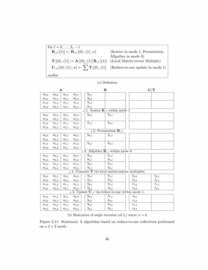
for ` = 0, . . . , I1 − 1B:,` [(1)]← B:,` [(0) ; (1) , w] (Scatter in mode 1, Permutation,

Allgather in mode 0)T [(0) , (1)] := A [(0) , (1)] B:,` [(1)] (Local Matrix-vector Multiply)

C:,` [(0) ; (1) , w]←∑

T [(0) , (1)] (Reduce-to-one update in mode 1)

endfor

(a) Definition

A B C/Ta0,0 a0,2 a0,1 a0,3 b0,`a2,0 a2,2 a2,1 a2,3 b2,`a1,0 a1,2 a1,1 a1,3 b1,`a3,0 a3,2 a3,1 a3,3 b3,`

↓ 1. Scatter B:,` within mode 1.a0,0 a0,2 a0,1 a0,3 b0,` b2,`a2,0 a2,2 a2,1 a2,3a1,0 a1,2 a1,1 a1,3 b1,` b3,`a3,0 a3,2 a3,1 a3,3

↓ 2. Permutation B:,`.a0,0 a0,2 a0,1 a0,3 b0,` b1,`a2,0 a2,2 a2,1 a2,3a1,0 a1,2 a1,1 a1,3 b2,` b3,`a3,0 a3,2 a3,1 a3,3

↓ 3. Allgather B:,` within mode 0.a0,0 a0,2 a0,1 a0,3 b0,` b1,`a2,0 a2,2 a2,1 a2,3 b2,` b3,`a1,0 a1,2 a1,1 a1,3 b0,` b1,`a3,0 a3,2 a3,1 a3,3 b2,` b3,`

↓ 4. Compute T via local matrix-matrix multiplies.a0,0 a0,2 a0,1 a0,3 b0,` b1,` t0,0 t0,1a2,0 a2,2 a2,1 a2,3 b2,` b3,` t2,0 t2,1a1,0 a1,2 a1,1 a1,3 b0,` b1,` t1,0 t1,1a3,0 a3,2 a3,1 a3,3 b2,` b3,` t3,0 t3,1

↓ 5. Update C:,` via reduce-to-one within mode 1.a0,0 a0,2 a0,1 a0,3 b0,` b1,` c0,`a2,0 a2,2 a2,1 a2,3 b2,` b3,` c2,`a1,0 a1,2 a1,1 a1,3 b0,` b1,` c1,`a3,0 a3,2 a3,1 a3,3 b2,` b3,` c3,`

(b) Illustration of single iteration (of I1) where w = 0

Figure 2.11: Stationary A algorithm based on reduce-to-one collectives performedon a 2× 2 mesh.

46

We use the notation∑ιη

to indicate a contraction that is to be performed via a

collective that communicates over modes of the processing mesh used to distribute

the tensor modes labeled ι and η. Similarly, we use the location∑ιη

to indicate

a contraction that is to be performed locally by each process. We omit the spe-

cific labels to perform a contraction over when it is clear from the computation

which modes are being contracted (for instance when computing a matrix-matrix

multiplication).

Note that the reason for the final global reduction stems from the fact that, during

the parallel matrix-vector multiplication, no process is assigned all indices of the

mode involved in the summation. This means that no process can fully compute the

locally stored portion of C:,u and therefore a reduction of elements across processes

is required to accumulate the local contributions. This is the same reason for the

introduction of the (temporary) matrix T.

47

Under the assumed cost model, this algorithm has a cost of

2I0I1I2p

+ I1

(log2 (P1)α+

P1 − 1

P1

I2P0β

)︸ ︷︷ ︸

Scatter B:,u in mode 1

+ I1

(α+

I2P0P1

β

)︸ ︷︷ ︸

Permutation B:,u

+ I1

(log2 (P0)α+ (P0 − 1)

I2P0P1

β

)︸ ︷︷ ︸

Allgather B:,u in mode 0

+ I1

(log2 (P1)α+

I0P0β

)︸ ︷︷ ︸

Reduce-to-one T in mode 1

= 2I0I1I2p

+ I1 (log2 (p) + P1 + 1)α

+(P0 + P1 − 1) I2 + P1I0

pI1β.

(2.6)

Once again, if additional memory is available to perform the computation, we rec-

ognize that the series of scatter collectives (with different root processes) can be im-

plemented as an all-to-all, the series of permutation collectives can be implemented

as a single permutation, the series of allgather collectives can be implemented as a

single allgather (on more data), and the series of reduce-to-one collectives (with dif-

ferent root processes) can be implemented as a reduce-scatter. Further, the series of

matrix-vector multiplications can be implemented as a single matrix-matrix multipli-

cation that, instead of forming a matrix T, forms an order-3 tensor T. In Chapter 3

we discuss the origin of T. The algorithm resulting from this series of refactorings,

along with an illustration of the algorithm, is given in Figure 2.12.

48

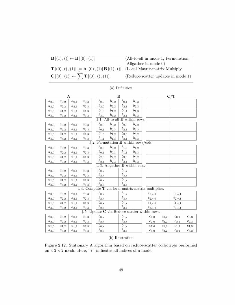
B [(1) , ()]← B [(0) , (1)] (All-to-all in mode 1, Permutation,Allgather in mode 0)

T [(0) , () , (1)] := A [(0) , (1)] B [(1) , ()] (Local Matrix-matrix Multiply

C [(0) , (1)]←∑

T [(0) , () , (1)] (Reduce-scatter updates in mode 1)

(a) Definition

A B C/Ta0,0 a0,2 a0,1 a0,3 b0,0 b0,2 b0,1 b0,3a2,0 a2,2 a2,1 a2,3 b2,0 b2,2 b2,1 b2,3a1,0 a1,2 a1,1 a1,3 b1,0 b1,2 b1,1 b1,3a3,0 a3,2 a3,1 a3,3 b3,0 b3,2 b3,1 b3,3

↓ 1. All-to-all B within rows.a0,0 a0,2 a0,1 a0,3 b0,0 b0,2 b2,0 b2,2a2,0 a2,2 a2,1 a2,3 b0,1 b0,3 b2,1 b2,3a1,0 a1,2 a1,1 a1,3 b1,0 b1,2 b3,0 b3,2a3,0 a3,2 a3,1 a3,3 b1,1 b1,3 b3,1 b3,3

↓ 2. Permutation B within rows/cols.a0,0 a0,2 a0,1 a0,3 b0,0 b0,2 b1,0 b1,2a2,0 a2,2 a2,1 a2,3 b0,1 b0,3 b1,1 b1,3a1,0 a1,2 a1,1 a1,3 b2,0 b2,2 b3,0 b3,2a3,0 a3,2 a3,1 a3,3 b2,1 b2,3 b3,1 b3,3

↓ 3. Allgather B within cols.a0,0 a0,2 a0,1 a0,3 b0,∗ b1,∗a2,0 a2,2 a2,1 a2,3 b2,∗ b3,∗a1,0 a1,2 a1,1 a1,3 b0,∗ b1,∗a3,0 a3,2 a3,1 a3,3 b2,∗ b3,∗

↓ 4. Compute T via local matrix-matrix multiplies.a0,0 a0,2 a0,1 a0,3 b0,∗ b1,∗ t0,∗,0 t0,∗,1a2,0 a2,2 a2,1 a2,3 b2,∗ b3,∗ t2,∗,0 t2,∗,1a1,0 a1,2 a1,1 a1,3 b0,∗ b1,∗ t1,∗,0 t1,∗,1a3,0 a3,2 a3,1 a3,3 b2,∗ b3,∗ t3,∗,0 t3,∗,1

↓ 5. Update C via Reduce-scatter within rows.a0,0 a0,2 a0,1 a0,3 b0,∗ b1,∗ c0,0 c0,2 c0,1 c0,3a2,0 a2,2 a2,1 a2,3 b2,∗ b3,∗ c2,0 c2,2 c2,1 c2,3a1,0 a1,2 a1,1 a1,3 b0,∗ b1,∗ c1,0 c1,2 c1,1 c1,3a3,0 a3,2 a3,1 a3,3 b2,∗ b3,∗ c3,0 c3,2 c3,1 c3,3

(b) Illustration

Figure 2.12: Stationary A algorithm based on reduce-scatter collectives performedon a 2× 2 mesh. Here, “∗” indicates all indices of a mode.

49

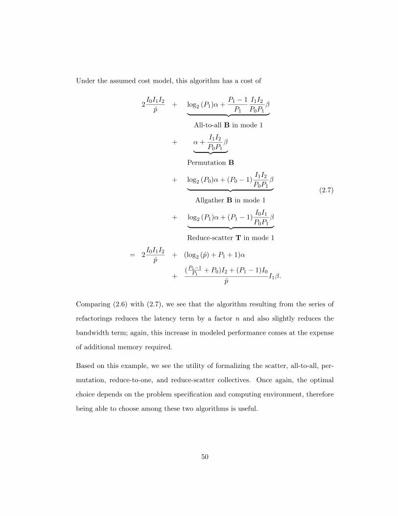
Under the assumed cost model, this algorithm has a cost of

2I0I1I2p

+ log2 (P1)α+P1 − 1

P1

I1I2P0P1

β︸ ︷︷ ︸All-to-all B in mode 1

+ α+I1I2P0P1

β︸ ︷︷ ︸Permutation B

+ log2 (P0)α+ (P0 − 1)I1I2P0P1

β︸ ︷︷ ︸Allgather B in mode 1

+ log2 (P1)α+ (P1 − 1)I0I1P0P1

β︸ ︷︷ ︸Reduce-scatter T in mode 1

= 2I0I1I2p

+ (log2 (p) + P1 + 1)α

+(P1−1P1

+ P0)I2 + (P1 − 1)I0

pI1β.

(2.7)

Comparing (2.6) with (2.7), we see that the algorithm resulting from the series of

refactorings reduces the latency term by a factor n and also slightly reduces the

bandwidth term; again, this increase in modeled performance comes at the expense

of additional memory required.

Based on this example, we see the utility of formalizing the scatter, all-to-all, per-

mutation, reduce-to-one, and reduce-scatter collectives. Once again, the optimal

choice depends on the problem specification and computing environment, therefore

being able to choose among these two algorithms is useful.

50

2.5.3 Example: Allreduce and Gather-to-one

Up to now, we have provided evidence for the utility of all collectives considered

except for the allreduce, and gather-to-one collectives. The benefits of the allreduce

and gather-to-one collectives do not easily manifest when only considering a sin-

gle matrix-matrix operation. However, when considering a series of matrix-matrix

multiplications, such as

C = AB (2.8)

followed by

E = (AB)︸ ︷︷ ︸C

D + E (2.9)

where E is an I0 × I1 matrix, C is an I0 × I2 matrix, A is an I0 × I3 matrix,

and both matrices B and D are of conformal size, the utility of both allreduce and

gather-to-one collectives becomes more readily apparent. The relative sizes of the

matrices involved to demonstrate the utility of both the allreduce and gather-to-one

collectives are given in Figure 2.13.

To see the utility of the allreduce collective, consider the case where I2 is small rela-

tive to all other dimensions (Figure 2.13a). Applying what we discussed in previous

subsections concerning stationary algorithmic variants, we recognize that a station-

ary A algorithm is appropriate for computing (2.8), while a stationary C algorithm

is appropriate for computing (2.9) as these algorithms do not communicate the

“large” operand in the associated matrix-matrix multiplication. An examination of

51

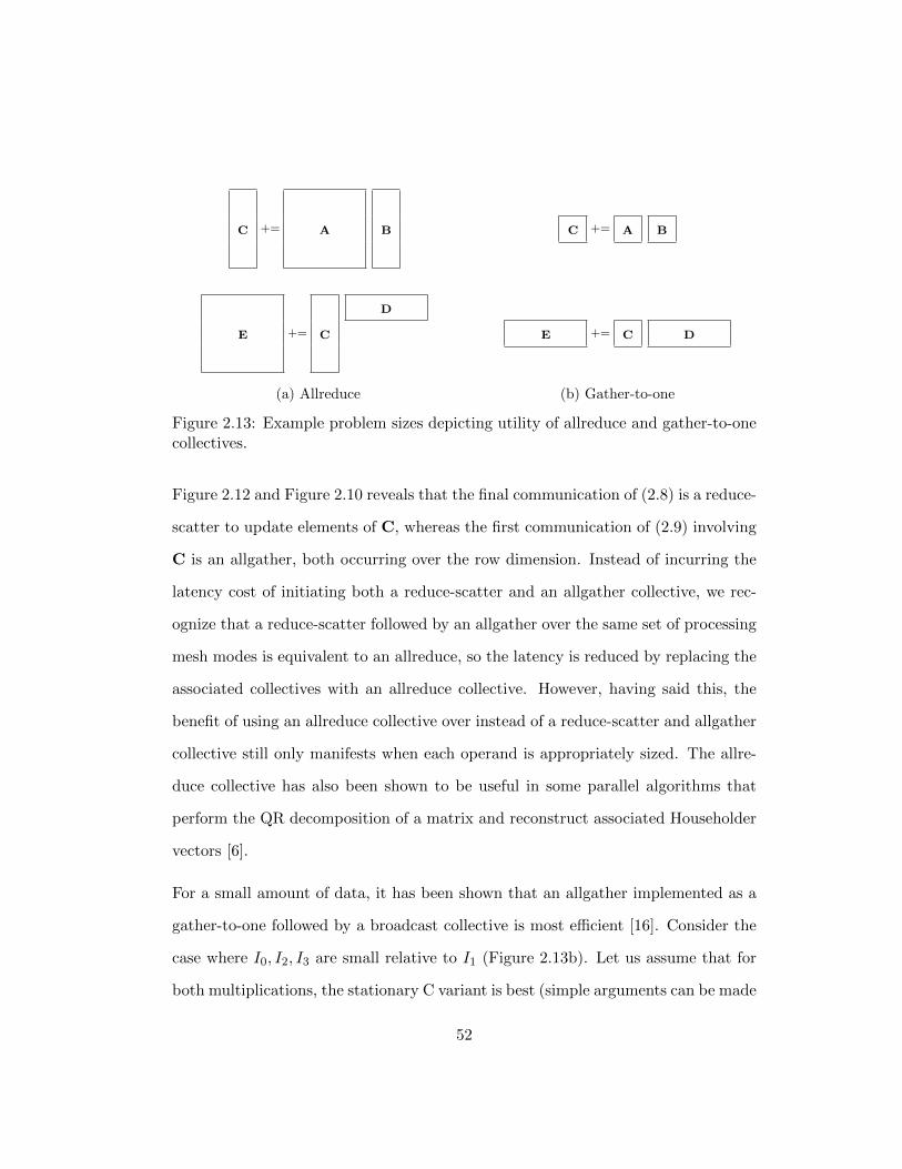
C += A B

E += C

D

(a) Allreduce

C += A B

E += C D

(b) Gather-to-one

Figure 2.13: Example problem sizes depicting utility of allreduce and gather-to-onecollectives.

Figure 2.12 and Figure 2.10 reveals that the final communication of (2.8) is a reduce-

scatter to update elements of C, whereas the first communication of (2.9) involving

C is an allgather, both occurring over the row dimension. Instead of incurring the

latency cost of initiating both a reduce-scatter and an allgather collective, we rec-

ognize that a reduce-scatter followed by an allgather over the same set of processing

mesh modes is equivalent to an allreduce, so the latency is reduced by replacing the

associated collectives with an allreduce collective. However, having said this, the

benefit of using an allreduce collective over instead of a reduce-scatter and allgather

collective still only manifests when each operand is appropriately sized. The allre-

duce collective has also been shown to be useful in some parallel algorithms that

perform the QR decomposition of a matrix and reconstruct associated Householder

vectors [6].

For a small amount of data, it has been shown that an allgather implemented as a

gather-to-one followed by a broadcast collective is most efficient [16]. Consider the

case where I0, I2, I3 are small relative to I1 (Figure 2.13b). Let us assume that for

both multiplications, the stationary C variant is best (simple arguments can be made

52

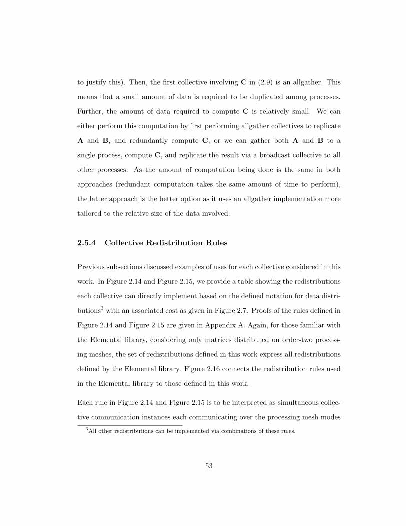
to justify this). Then, the first collective involving C in (2.9) is an allgather. This

means that a small amount of data is required to be duplicated among processes.

Further, the amount of data required to compute C is relatively small. We can

either perform this computation by first performing allgather collectives to replicate

A and B, and redundantly compute C, or we can gather both A and B to a

single process, compute C, and replicate the result via a broadcast collective to all

other processes. As the amount of computation being done is the same in both

approaches (redundant computation takes the same amount of time to perform),

the latter approach is the better option as it uses an allgather implementation more

tailored to the relative size of the data involved.

2.5.4 Collective Redistribution Rules

Previous subsections discussed examples of uses for each collective considered in this

work. In Figure 2.14 and Figure 2.15, we provide a table showing the redistributions

each collective can directly implement based on the defined notation for data distri-

butions3 with an associated cost as given in Figure 2.7. Proofs of the rules defined in

Figure 2.14 and Figure 2.15 are given in Appendix A. Again, for those familiar with

the Elemental library, considering only matrices distributed on order-two process-

ing meshes, the set of redistributions defined in this work express all redistributions

defined by the Elemental library. Figure 2.16 connects the redistribution rules used

in the Elemental library to those defined in this work.

Each rule in Figure 2.14 and Figure 2.15 is to be interpreted as simultaneous collec-

tive communication instances each communicating over the processing mesh modes

3All other redistributions can be implemented via combinations of these rules.

53

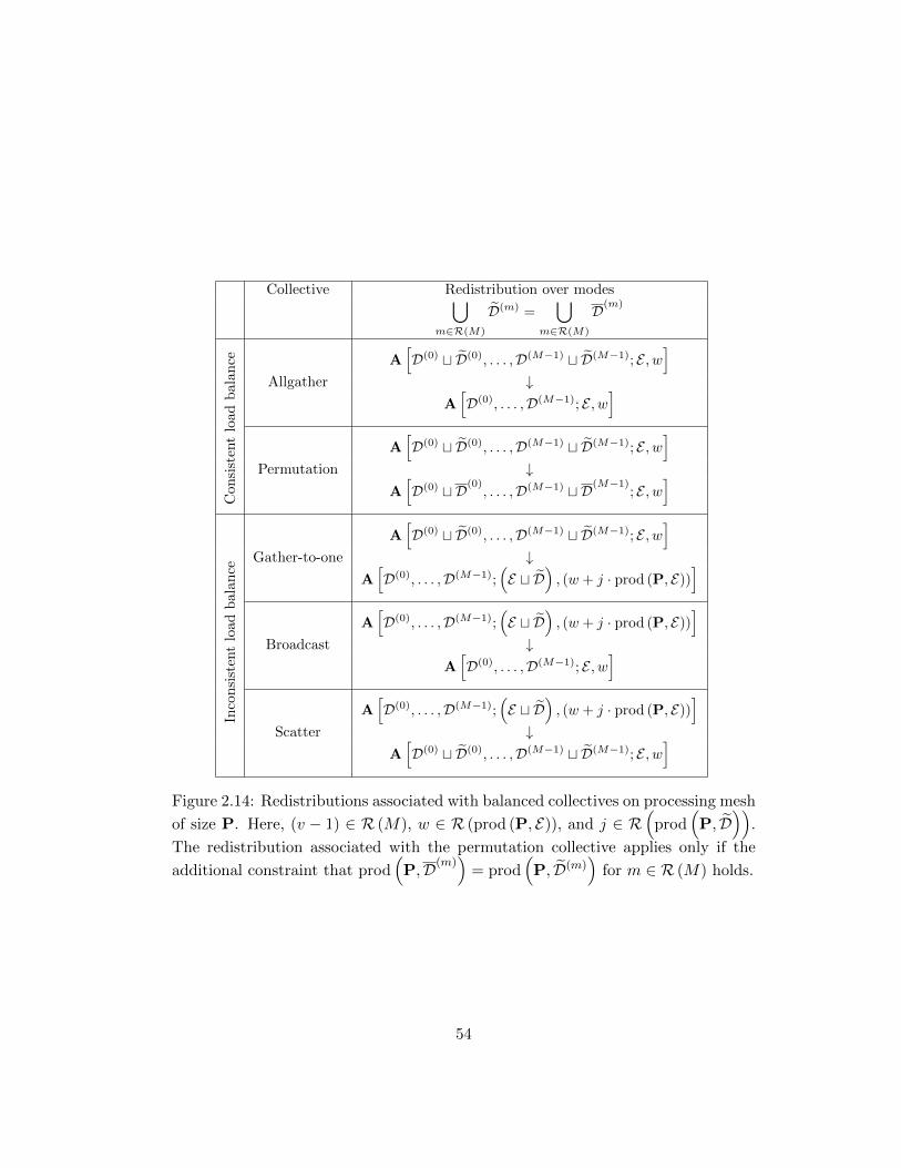
Collective Redistribution over modes⋃m∈R(M)

D(m) =⋃

m∈R(M)

D(m)

Con

sist

ent

load

bal

ance A

[D(0) t D(0), . . . ,D(M−1) t D(M−1); E , w

]Allgather ↓

A[D(0), . . . ,D(M−1); E , w

]A[D(0) t D(0), . . . ,D(M−1) t D(M−1); E , w

]Permutation ↓

A[D(0) t D(0)

, . . . ,D(M−1) t D(M−1); E , w

]

Inco

nsi

sten

tlo

adb

ala

nce

A[D(0) t D(0), . . . ,D(M−1) t D(M−1); E , w

]Gather-to-one ↓

A[D(0), . . . ,D(M−1);

(E t D

), (w + j · prod (P, E))

]A[D(0), . . . ,D(M−1);

(E t D

), (w + j · prod (P, E))

]Broadcast ↓

A[D(0), . . . ,D(M−1); E , w

]A[D(0), . . . ,D(M−1);

(E t D

), (w + j · prod (P, E))

]Scatter ↓

A[D(0) t D(0), . . . ,D(M−1) t D(M−1); E , w

]Figure 2.14: Redistributions associated with balanced collectives on processing mesh

of size P. Here, (v − 1) ∈ R (M), w ∈ R (prod (P, E)), and j ∈ R(

prod(P, D

)).

The redistribution associated with the permutation collective applies only if the

additional constraint that prod(P,D(m)

)= prod

(P, D(m)

)for m ∈ R (M) holds.

54

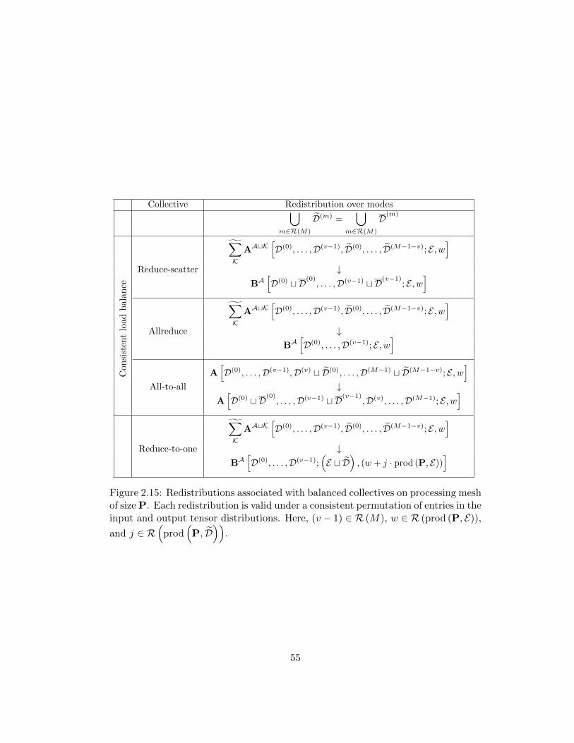
Collective Redistribution over modes⋃m∈R(M)

D(m) =⋃

m∈R(M)

D(m)

Con

sist

ent

load

bal

ance

∑K

AAtK[D(0), . . . ,D(v−1), D(0), . . . , D(M−1−v); E , w

]Reduce-scatter ↓

BA[D(0) t D(0)

, . . . ,D(v−1) t D(v−1); E , w

]∑K

AAtK[D(0), . . . ,D(v−1), D(0), . . . , D(M−1−v); E , w

]Allreduce ↓

BA[D(0), . . . ,D(v−1); E , w

]A[D(0), . . . ,D(v−1),D(v) t D(0), . . . ,D(M−1) t D(M−1−v); E , w

]All-to-all ↓

A[D(0) t D(0)

, . . . ,D(v−1) t D(v−1),D(v), . . . ,D(M−1); E , w

]∑K

AAtK[D(0), . . . ,D(v−1), D(0), . . . , D(M−1−v); E , w

]Reduce-to-one ↓

BA[D(0), . . . ,D(v−1);

(E t D

), (w + j · prod (P, E))

]Figure 2.15: Redistributions associated with balanced collectives on processing meshof size P. Each redistribution is valid under a consistent permutation of entries in theinput and output tensor distributions. Here, (v − 1) ∈ R (M), w ∈ R (prod (P, E)),

and j ∈ R(

prod(P, D

)).

55

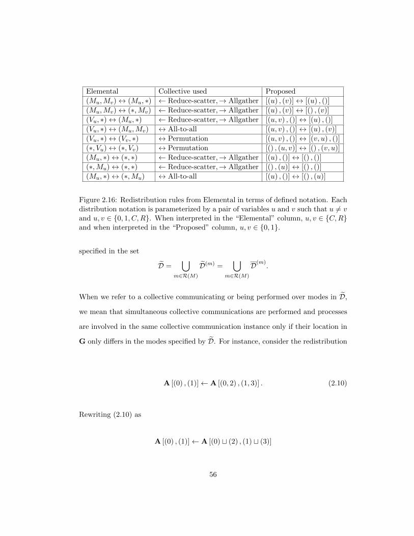
Elemental Collective used Proposed

(Mu,Mv)↔ (Mu, ∗) ← Reduce-scatter,→ Allgather [(u) , (v)]↔ [(u) , ()]

(Mu,Mv)↔ (∗,Mv) ← Reduce-scatter,→ Allgather [(u) , (v)]↔ [() , (v)]

(Vu, ∗)↔ (Mu, ∗) ← Reduce-scatter,→ Allgather [(u, v) , ()]↔ [(u) , ()]

(Vu, ∗)↔ (Mu,Mv) ↔ All-to-all [(u, v) , ()]↔ [(u) , (v)]

(Vu, ∗)↔ (Vv, ∗) ↔ Permutation [(u, v) , ()]↔ [(v, u) , ()]

(∗, Vu)↔ (∗, Vv) ↔ Permutation [() , (u, v)]↔ [() , (v, u)]

(Mu, ∗)↔ (∗, ∗) ← Reduce-scatter,→ Allgather [(u) , ()]↔ [() , ()]

(∗,Mu)↔ (∗, ∗) ← Reduce-scatter,→ Allgather [() , (u)]↔ [() , ()]

(Mu, ∗)↔ (∗,Mu) ↔ All-to-all [(u) , ()]↔ [() , (u)]

Figure 2.16: Redistribution rules from Elemental in terms of defined notation. Eachdistribution notation is parameterized by a pair of variables u and v such that u 6= vand u, v ∈ {0, 1, C,R}. When interpreted in the “Elemental” column, u, v ∈ {C,R}and when interpreted in the “Proposed” column, u, v ∈ {0, 1}.

specified in the set

D =⋃

m∈R(M)

D(m) =⋃

m∈R(M)

D(m).

When we refer to a collective communicating or being performed over modes in D,

we mean that simultaneous collective communications are performed and processes

are involved in the same collective communication instance only if their location in

G only differs in the modes specified by D. For instance, consider the redistribution

A [(0) , (1)]← A [(0, 2) , (1, 3)] . (2.10)

Rewriting (2.10) as

A [(0) , (1)]← A [(0) t (2) , (1) t (3)]

56

and consulting Figure 2.14 and Figure 2.15 reveals that the redistribution corre-

sponds to an allgather collective communicating over modes D = (2, 3) (as D(0) = (2)

and D(1) = (3)).

Interestingly, and importantly, all redistributions affect the ends, or suffixes of tensor

mode distributions. The reason for this becomes apparent when one considers the

definition of how elements are distributed among processes in conjunction with the

set of processing mesh modes over which communication occurs.

Other collectives have more flexible rules. In the case of the permutation collective,

the final tensor mode distributions “shuffle” entries of the initial mode distributions.

For example, the redistribution

A [(2, 0) , (1)]← A [(0, 2) , (1)] (2.11)

can be performed via a permutation collective communicating over the group of

processing mesh modes in (0, 2).

The absolute limit of flexibility in collectives comes with the all-to-all collective.

This flexibility allows an all-to-all collective to implement all other collectives that

do not perform a reduction of data being communicated (permutation, allgather,

gather-to-one, scatter, and broadcast). For example, both (2.10) and (2.11) can be

implemented as an all-to-all. Intuitively, this makes sense as an all-to-all collec-

tive can send some data to all processes involved in the communication; different

output distributions are created depending on how the data is ordered when redis-

tributed.

In practice it is typically better to use the more specialized collectives to perform

57

these redistributions as the all-to-all collective required is typically “unbalanced”,

and would result in a significantly higher cost in terms of bandwidth to implement

the same redistribution. For instance, consider the case where we implement a

permutation collective in terms of an all-to-all collective. Each process needs only

to send data to one other process in the mesh and otherwise does not need to

communicate any data with other processes. This pattern is highly unbalanced

in terms of amount of actual data a single process needs to send to every other

process. To implement this in terms of an all-to-all, one would need to send an

set of “empty” data packets to every other process that would be ignored upon

reception. The problem lies in the fact that each of these “empty” data packets are

the same size as the actual data required to be exchanged.

2.6 Summary

Understanding how data is distributed on a processing mesh is the first step in de-

signing efficient implementations for computations of interest. However, one must

also understand how collective communications can be utilized to efficiently redis-

tribute data among processes. When these interactions are well understood, one

can design families of algorithms that achieve high-performance for computations.

In our case, we see how one can design such algorithms for tensor contractions, as

we will see next.

In this chapter, we introduced a notation for describing how data of an order-M

tensor is distributed among processes of an order-N mesh based on an elemental-

cyclic distribution. Additionally, we argued the utility of each collective depicted in

Figure 2.6 and formalized each collective as redistributions in the notation.

58

Chapter 3

Algorithm Derivation

Now that we have an understanding of the relationship between data distributions

and redistributions that can be cast in terms of collective communications, we can

discuss how the ideas in the previous chapter can be leveraged to design algorithms

for tensor computations with associated high-performance implementations. This

work focuses on generalizing the family of algorithms for matrix-matrix multiplica-

tion, introduced earlier in Chapter 2, to tensor contractions of dense non-symmetric

tensors.

We begin this chapter by first introducing the general structure of our derivation

procedure followed by discussing several examples based on this approach to build

an intuition. Subsequently, we formalize the procedure. We restrict the discus-

sion in this chapter to binary contractions, although the ideas generalize to n-ary

contractions.

59

3.1 Preliminaries

3.1.1 Approach

Consider the general form of a binary tensor contraction given by

CC =∑K

AABB + CC (3.1)

where K = A ∩ B and the tensors A, B, and C are appropriately sized based on

how modes of each tensor are paired. Let I(K) =(I(K)0 , . . . , I

(K)|K|−1

)represent the

dimensions of the modes labeled K. Then, each element of C is defined as

ci(C) +=∑

k∈R(I(K))

ai(A) · bi(B) (3.2)

where i(A) and i(B) are consistently defined and therefore incorporate k in their

definition.

We can refactor the computation of (3.2) into two steps, where we first form a set

of temporaries each representing the result of a disjoint set of accumulations and

then sum the results into the output object. The observation allows each process in

our processing mesh to locally compute a portion of (3.2) and then collaborate with

other processes to form results together via a global communication (if necessary).

For consistency, the order of the introduced temporary, T, must be the same as the

output C plus the number of labels involved in the summation (|K|). This stems

from the fact that each process is computing independent portions of T that can be

60

accumulated into the output C. Considering this, we reformulate (3.1) as

TCtK′

=∑K

AABB (3.3)

CC =∑K′

TCtK′+ CC (3.4)

As mentioned, (3.3) does not represent a complete computation, only a partial

computation. We introduce K′ merely to indicate that the corresponding modes

have only been partially contracted and therefore must be eliminated in (3.4) (the

entries and corresponding order of K′ are the same as in K). The correct elementwise

definition of (3.3) and (3.4) is given by

ti(C)tp =∑k∈Pp

ai(A) · bi(B) (3.5)

ci(C) +=∑

k∈R(P)

ti(C)tk, (3.6)

where P forms a partition of R(I(K)

)into prod (P) sets (indexed by p) and both

i(A) and i(B) are appropriately defined. Using (3.5) and (3.6), the interpretations

of (3.3) and (3.4) are clear: we form the partial contributions in (3.3) and then

accumulate over the results in (3.4). Introducing T as a variable allows us to separate

computations to be performed locally by each process from the summation that must

be performed globally.

It should be noted that the refactoring chosen based on processes in a processing

mesh represents only one choice of many; nothing prevents us from computing (3.1)

in multiple steps instead of two as done here. Although there may be benefits to

further decomposing the computation to expose additional parallelism, such as that

61

exposed by so-called 3D algorithms for matrix-matrix multiplication [2, 41, 73, 79], in

this work we focus on decomposing into two steps as we develop a general framework.

Projects such as the Cyclops Tensor Framework (CTF) [81] and the RRR [70] already

leverage versions of these algorithms. Extending our framework to also incorporate

these insights is left as future work and is out of the scope of this document.

3.1.2 Distributed Template

To create an algorithm template for computing a binary tensor contraction based

on the ideas introduced in the previous subsection, we must introduce the notion of

data distributions into the discussion, transforming (3.3) and (3.4) into

TCtK′[D(T)

]=∑K

AA[D(A)

]BB[D(B)

](3.7)

CC[D(C)

]=∑K′

TCtK′[D(T)

]+ CC

[D(C)

]. (3.8)

where D(A), D(B)

, D(C), and D(T) represent the distributions of the associated

tensor at the time local computation is performed. Recall that the elementwise

definition of T in (3.5) and (3.6) is based on a partition of the computation to be

performed. The most natural partition to use is the one that assigns each process

all computations that can be performed locally at this point in the algorithm. In-

corporating this in (3.7) and (3.8) leads to the elementwise definition given by

ti(C)tp =∑

k∈I(p)(D(K))

ai(A) · bi(B) (3.9)

ci(C) +=∑

k∈R(P(D(K)))

ti(C)tk, (3.10)

62

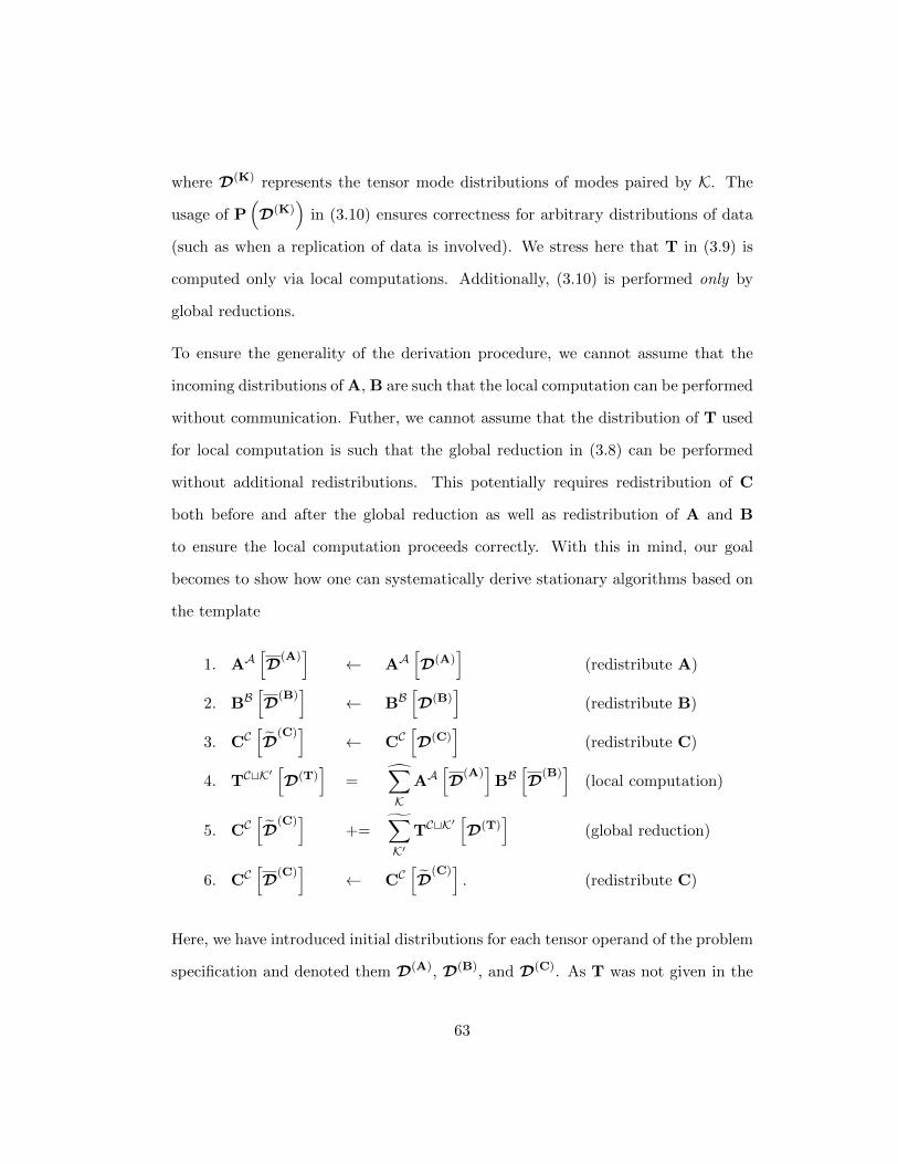
where D(K) represents the tensor mode distributions of modes paired by K. The

usage of P(D(K)

)in (3.10) ensures correctness for arbitrary distributions of data

(such as when a replication of data is involved). We stress here that T in (3.9) is

computed only via local computations. Additionally, (3.10) is performed only by

global reductions.

To ensure the generality of the derivation procedure, we cannot assume that the

incoming distributions of A, B are such that the local computation can be performed

without communication. Futher, we cannot assume that the distribution of T used

for local computation is such that the global reduction in (3.8) can be performed

without additional redistributions. This potentially requires redistribution of C

both before and after the global reduction as well as redistribution of A and B

to ensure the local computation proceeds correctly. With this in mind, our goal

becomes to show how one can systematically derive stationary algorithms based on

the template

1. AA[D(A)

]← AA

[D(A)

](redistribute A)

2. BB[D(B)

]← BB

[D(B)

](redistribute B)

3. CC[D

(C)]

← CC[D(C)

](redistribute C)

4. TCtK′[D(T)

]=

∑K

AA[D(A)

]BB[D(B)

](local computation)

5. CC[D

(C)]

+=∑K′

TCtK′[D(T)

](global reduction)

6. CC[D(C)

]← CC

[D

(C)]. (redistribute C)

Here, we have introduced initial distributions for each tensor operand of the problem

specification and denoted them D(A), D(B), and D(C). As T was not given in the

63

original problem specification, we are free to choose its distribution D(T). We

require the introduction of D(C)

to ensure the global reduction succeeds and the

introduction of D(C)to ensure the postcondition of our to be developed algorithm

is achieved.

With this template set, our goal now becomes to systematically determine the val-

ues for D(A), D(B), D(C), D(T) (initial tensor distributions), D(A), D(B)

, D(C)

(final tensor distributions), and D(C)

(intermediate distribution). We will see that

depending on the algorithmic variant being derived, some of these steps become

greatly simplified and some of these unknowns become predetermined. We now pro-

vide examples of how the derivation procedure proceeds for both the stationary C

and stationary A algorithmic variants before we formalize the procedure.

3.2 Example: Stationary C Algorithms

Consider the tensor contraction

Cαβηι = AαγικBβγηκ + Cαβηι

where C, A and B are conformally sized. For this example, our goal is to derive an

algorithm that computes the above expression without communicating C, yielding a

stationary C algorithm. Assume we are performing this computation on an order-4

processing mesh G of size P = (P0, P1, P2, P3).

64

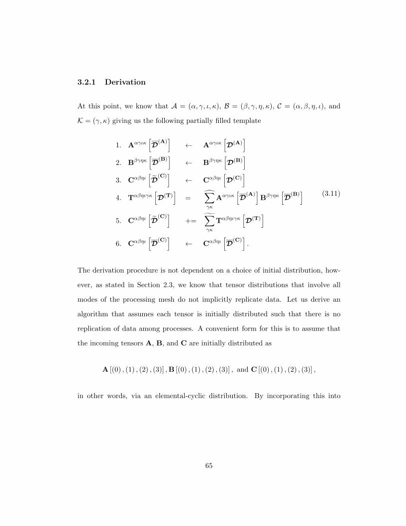
3.2.1 Derivation

At this point, we know that A = (α, γ, ι, κ), B = (β, γ, η, κ), C = (α, β, η, ι), and

K = (γ, κ) giving us the following partially filled template

1. Aαγικ[D(A)

]← Aαγικ

[D(A)

]2. Bβγηκ

[D(B)

]← Bβγηκ

[D(B)

]3. Cαβηι

[D

(C)]

← Cαβηι[D(C)

]4. Tαβηιγκ

[D(T)

]=

∑γκ

Aαγικ[D(A)

]Bβγηκ

[D(B)

]5. Cαβηι

[D

(C)]

+=∑γκ

Tαβηιγκ[D(T)

]6. Cαβηι

[D(C)

]← Cαβηι

[D(C)

].

(3.11)

The derivation procedure is not dependent on a choice of initial distribution, how-

ever, as stated in Section 2.3, we know that tensor distributions that involve all

modes of the processing mesh do not implicitly replicate data. Let us derive an

algorithm that assumes each tensor is initially distributed such that there is no

replication of data among processes. A convenient form for this is to assume that

the incoming tensors A, B, and C are initially distributed as

A [(0) , (1) , (2) , (3)] ,B [(0) , (1) , (2) , (3)] , and C [(0) , (1) , (2) , (3)] ,

in other words, via an elemental-cyclic distribution. By incorporating this into

65

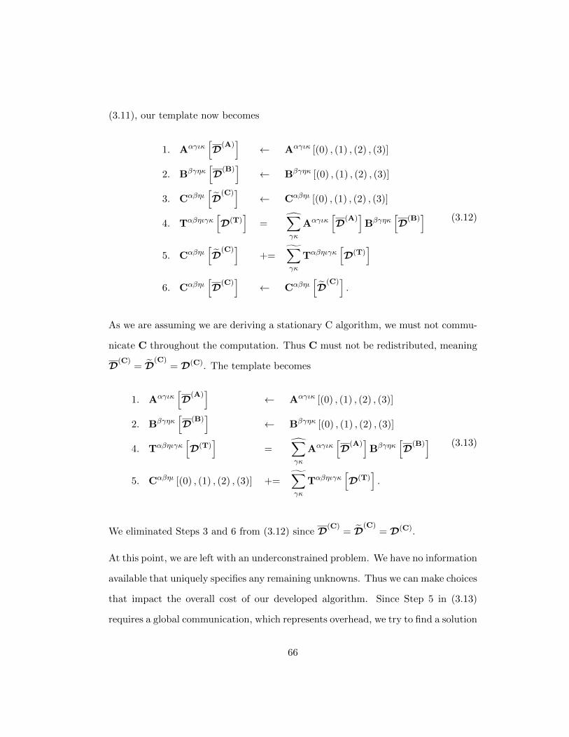
(3.11), our template now becomes

1. Aαγικ[D(A)

]← Aαγικ [(0) , (1) , (2) , (3)]

2. Bβγηκ[D(B)

]← Bβγηκ [(0) , (1) , (2) , (3)]

3. Cαβηι[D

(C)]

← Cαβηι [(0) , (1) , (2) , (3)]

4. Tαβηιγκ[D(T)

]=

∑γκ

Aαγικ[D(A)

]Bβγηκ

[D(B)

]5. Cαβηι

[D

(C)]

+=∑γκ

Tαβηιγκ[D(T)

]6. Cαβηι

[D(C)

]← Cαβηι

[D

(C)].

(3.12)

As we are assuming we are deriving a stationary C algorithm, we must not commu-

nicate C throughout the computation. Thus C must not be redistributed, meaning

D(C)= D

(C)= D(C). The template becomes

1. Aαγικ[D(A)

]← Aαγικ [(0) , (1) , (2) , (3)]

2. Bβγηκ[D(B)

]← Bβγηκ [(0) , (1) , (2) , (3)]

4. Tαβηιγκ[D(T)

]=

∑γκ

Aαγικ[D(A)

]Bβγηκ

[D(B)

]5. Cαβηι [(0) , (1) , (2) , (3)] +=

∑γκ

Tαβηιγκ[D(T)

].

(3.13)

We eliminated Steps 3 and 6 from (3.12) since D(C)= D

(C)= D(C).

At this point, we are left with an underconstrained problem. We have no information

available that uniquely specifies any remaining unknowns. Thus we can make choices

that impact the overall cost of our developed algorithm. Since Step 5 in (3.13)

requires a global communication, which represents overhead, we try to find a solution

66

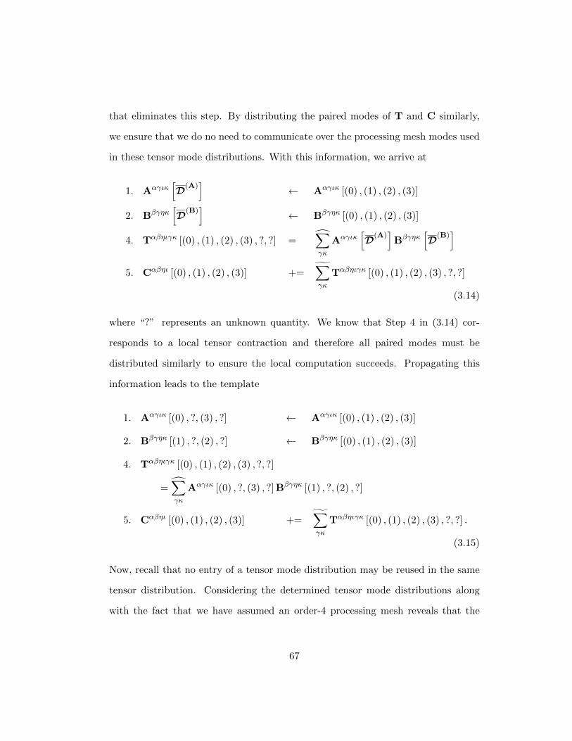
that eliminates this step. By distributing the paired modes of T and C similarly,

we ensure that we do no need to communicate over the processing mesh modes used

in these tensor mode distributions. With this information, we arrive at

1. Aαγικ[D(A)

]← Aαγικ [(0) , (1) , (2) , (3)]

2. Bβγηκ[D(B)

]← Bβγηκ [(0) , (1) , (2) , (3)]

4. Tαβηιγκ [(0) , (1) , (2) , (3) , ?, ?] =∑γκ

Aαγικ[D(A)

]Bβγηκ

[D(B)

]5. Cαβηι [(0) , (1) , (2) , (3)] +=

∑γκ

Tαβηιγκ [(0) , (1) , (2) , (3) , ?, ?]

(3.14)

where “?” represents an unknown quantity. We know that Step 4 in (3.14) cor-

responds to a local tensor contraction and therefore all paired modes must be

distributed similarly to ensure the local computation succeeds. Propagating this

information leads to the template

1. Aαγικ [(0) , ?, (3) , ?] ← Aαγικ [(0) , (1) , (2) , (3)]

2. Bβγηκ [(1) , ?, (2) , ?] ← Bβγηκ [(0) , (1) , (2) , (3)]

4. Tαβηιγκ [(0) , (1) , (2) , (3) , ?, ?]

=∑γκ

Aαγικ [(0) , ?, (3) , ?] Bβγηκ [(1) , ?, (2) , ?]

5. Cαβηι [(0) , (1) , (2) , (3)] +=∑γκ

Tαβηιγκ [(0) , (1) , (2) , (3) , ?, ?] .

(3.15)

Now, recall that no entry of a tensor mode distribution may be reused in the same

tensor distribution. Considering the determined tensor mode distributions along

with the fact that we have assumed an order-4 processing mesh reveals that the

67

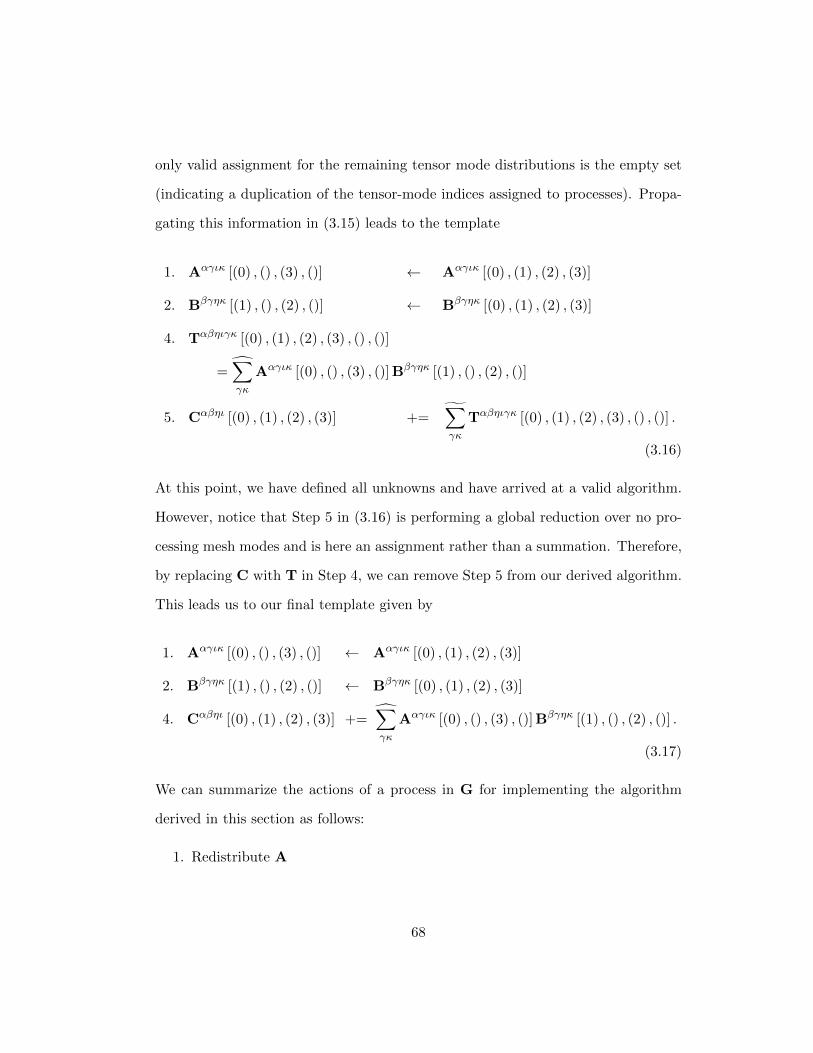
only valid assignment for the remaining tensor mode distributions is the empty set

(indicating a duplication of the tensor-mode indices assigned to processes). Propa-

gating this information in (3.15) leads to the template

1. Aαγικ [(0) , () , (3) , ()] ← Aαγικ [(0) , (1) , (2) , (3)]

2. Bβγηκ [(1) , () , (2) , ()] ← Bβγηκ [(0) , (1) , (2) , (3)]

4. Tαβηιγκ [(0) , (1) , (2) , (3) , () , ()]

=∑γκ

Aαγικ [(0) , () , (3) , ()] Bβγηκ [(1) , () , (2) , ()]

5. Cαβηι [(0) , (1) , (2) , (3)] +=∑γκ

Tαβηιγκ [(0) , (1) , (2) , (3) , () , ()] .

(3.16)

At this point, we have defined all unknowns and have arrived at a valid algorithm.

However, notice that Step 5 in (3.16) is performing a global reduction over no pro-

cessing mesh modes and is here an assignment rather than a summation. Therefore,

by replacing C with T in Step 4, we can remove Step 5 from our derived algorithm.

This leads us to our final template given by

1. Aαγικ [(0) , () , (3) , ()] ← Aαγικ [(0) , (1) , (2) , (3)]

2. Bβγηκ [(1) , () , (2) , ()] ← Bβγηκ [(0) , (1) , (2) , (3)]

4. Cαβηι [(0) , (1) , (2) , (3)] +=∑γκ

Aαγικ [(0) , () , (3) , ()] Bβγηκ [(1) , () , (2) , ()] .

(3.17)

We can summarize the actions of a process in G for implementing the algorithm

derived in this section as follows:

1. Redistribute A

68

2. Redistribute B

3. Locally compute ci(C) +=∑γκ

ai(A) · bi(B)

where i(A) and i(B) are appropriately defined. An examination of (3.17) reveals that

none of the required redistributions are directly implemented by the rules given in

Figure 2.14 and Figure 2.15. This is where expert knowledge is still required to

determine the optimal path of redistributions (minimal cost or storage). However,

the derivation procedure has significantly reduced the number of possibilities that

need to be considered.

3.2.2 Blocking

In Step 4 of (3.17), the distributions of A and B indicate a replication of data among

processes as some modes of G are not used in the associated tensor distribution. As

we increase the number of processes involved, so does the amount of data replication,

with associated memory requirements for the duplicated data. One straightforward

approach to curb this effect is to block the overall tensor contraction into a series

of smaller block tensor contractions to which we can apply the same derivation

process.

Depending on how we choose the size of each block, different characteristics of the

execution will be observed. If a large block size is chosen, a large amount of data is

required to perform the computation. If a small block size is chosen, reducing the

amount of storage required, a higher communication cost is predicted due to the

increased number of communications being performed (one round for each block).

It is this trade-off associated with the block size parameter that we must recognize

and appropriately analyze to ensure an efficient implementation is created.

69

Since we are dealing with higher-order tensors, determining the correct modes to

block may seem daunting at first. Observe that the source of replicated data in

(3.17) are the distributed tensors A [(0) , () , (3) , ()] and B [(1) , () , (2) , ()]. Com-

paring the distributions of these tensors to the initial distributions, we see that the

replication of data originates from the redistribution of the tensor modes involved in

the summation. If we increase the number of processes in our processing mesh, then

replication will occur due to the redistribution of these tensor modes. By blocking

along these modes, we can mitigate this effect.

Generalizing this observation, notice that the tensor modes we should block along

in (3.17) correspond to the modes that are unpaired with our stationary tensor C.

In fact, for all stationary variants, the observation that replication occurs due to the

redistribution of tensor modes not paired with the stationary operand and should be

blocked holds. This reasoning provides an expert with a simple way of determining

along which tensor modes to introduce blocking, thereby mitigating the increased

storage effect as the size of the processing mesh increases.

3.2.3 Observations

It may seem convenient that the remaining tensor mode distributions of A and B

were “forced” into a particular definition by assuming we were computing on an

order-4 grid. As discussed previously, if we arrive at a state where the subsequent

step is ambiguous, a choice must be made that leads to different algorithms with

different performance characteristics. This concern is equivalent to that of having

assumed an initial distribution. This was a heuristic, but is not necessarily the best

for every problem specification, especially when more than a binary contraction is

encountered.

70

Our goal in this work is to be able to formalize the derivation procedure to such a

degree that making these choices requires less effort by the (human or mechanical)

expert. By having such a systematic procedure for arriving at a valid algorithm

along with a well-defined notation, an expert can instantly detect along which modes

communication must occur. If the expert decides that a different set of assumptions

should be used, the same rote procedure can be applied to arrive at an algorithm

that is better suited under new sets of assumptions.

We now perform the same derivation for stationary A variants before generalizing

the procedure.

3.3 Example: Stationary A Algorithms

We again consider the tensor contraction

Cαβηι = AαγικBβγηκ + Cαβηι

only now we assume that we are deriving an algorithm that does not communicate

A.

3.3.1 Derivation

Assuming the same information regarding processing mesh configuration, initial

distributions, and the new information that we are deriving the stationary A variant,

71

we arrive at the following partially filled algorithm template

2. Bβγηκ [() , (1) , () , (3)] ← Bβγηκ [(0) , (1) , (2) , (3)]

3. Cαβηι[D

(C)]

← Cαβηι [(0) , (1) , (2) , (3)]

4. Tαβηιγκ [(0) , () , () , (2) , (1) , (3)]

=∑γκ

Aαγικ [(0) , (1) , (2) , (3)] Bβγηκ [() , (1) , () , (3)]

5. Cαβηι[D

(C)]

+=∑γκ

Tαβηιγκ [(0) , () , () , (2) , (1) , (3)]

6. Cαβηι[D(C)

]← Cαβηι

[D

(C)].

(3.18)

At this point, there are no further constraints we can apply to determine the def-

inition of D(C)or D

(C). For D

(C), we cannot assume that paired modes must be

distributed similarly as this distribution is used in a global reduction (not a local ten-

sor contraction). Further, we have no information available to constrain D(C). This

is a case where additional information or heuristics are required and performance

characteristics may vary depending on the choice made.

A common choice of D(C)is based on the assumption that the algorithm being

derived will be implemented in a loop structure; i.e., this is part of a blocked com-

putation. In this case, it is useful to have D(C)= D(C) as this eliminates one

source of redistribution between loop iterations. We adopt this heuristic for this

example. Once again, this is a choice made for example purposes only. Propagating

72

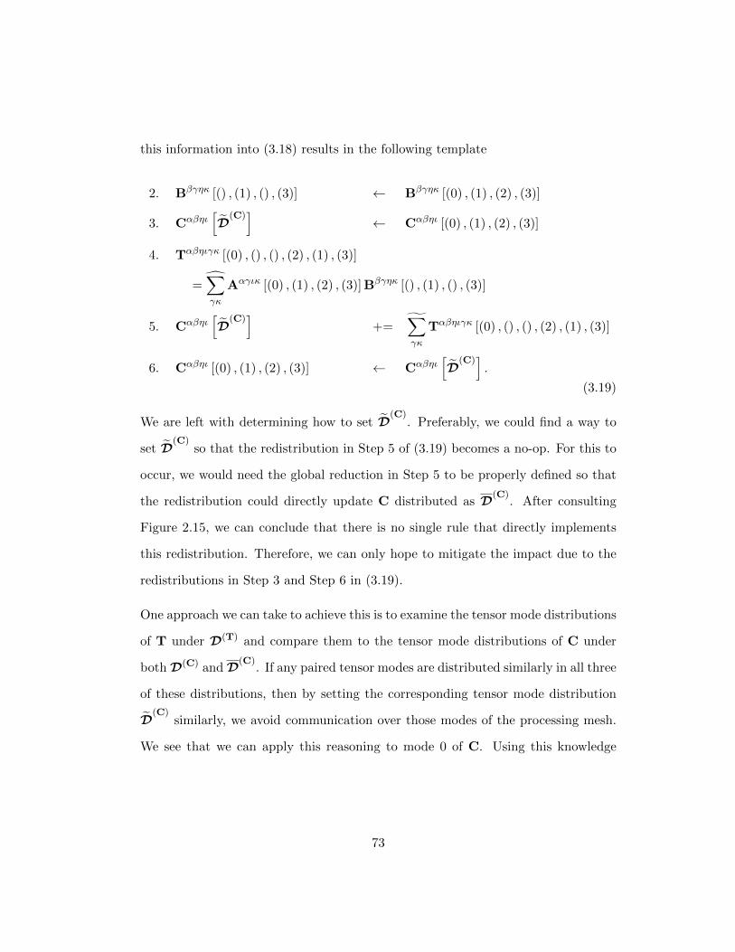
this information into (3.18) results in the following template

2. Bβγηκ [() , (1) , () , (3)] ← Bβγηκ [(0) , (1) , (2) , (3)]

3. Cαβηι[D

(C)]

← Cαβηι [(0) , (1) , (2) , (3)]

4. Tαβηιγκ [(0) , () , () , (2) , (1) , (3)]

=∑γκ

Aαγικ [(0) , (1) , (2) , (3)] Bβγηκ [() , (1) , () , (3)]

5. Cαβηι[D

(C)]

+=∑γκ

Tαβηιγκ [(0) , () , () , (2) , (1) , (3)]

6. Cαβηι [(0) , (1) , (2) , (3)] ← Cαβηι[D

(C)].

(3.19)

We are left with determining how to set D(C)

. Preferably, we could find a way to

set D(C)

so that the redistribution in Step 5 of (3.19) becomes a no-op. For this to

occur, we would need the global reduction in Step 5 to be properly defined so that

the redistribution could directly update C distributed as D(C). After consulting

Figure 2.15, we can conclude that there is no single rule that directly implements

this redistribution. Therefore, we can only hope to mitigate the impact due to the

redistributions in Step 3 and Step 6 in (3.19).

One approach we can take to achieve this is to examine the tensor mode distributions

of T under D(T) and compare them to the tensor mode distributions of C under

both D(C) and D(C). If any paired tensor modes are distributed similarly in all three

of these distributions, then by setting the corresponding tensor mode distribution

D(C)

similarly, we avoid communication over those modes of the processing mesh.

We see that we can apply this reasoning to mode 0 of C. Using this knowledge

73

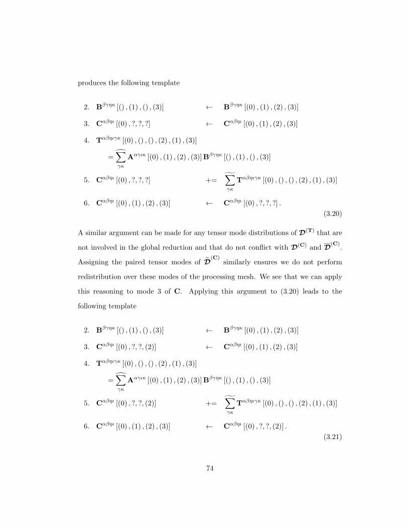
produces the following template

2. Bβγηκ [() , (1) , () , (3)] ← Bβγηκ [(0) , (1) , (2) , (3)]

3. Cαβηι [(0) , ?, ?, ?] ← Cαβηι [(0) , (1) , (2) , (3)]

4. Tαβηιγκ [(0) , () , () , (2) , (1) , (3)]

=∑γκ

Aαγικ [(0) , (1) , (2) , (3)] Bβγηκ [() , (1) , () , (3)]

5. Cαβηι [(0) , ?, ?, ?] +=∑γκ

Tαβηιγκ [(0) , () , () , (2) , (1) , (3)]

6. Cαβηι [(0) , (1) , (2) , (3)] ← Cαβηι [(0) , ?, ?, ?] .

(3.20)

A similar argument can be made for any tensor mode distributions of D(T) that are

not involved in the global reduction and that do not conflict with D(C) and D(C).

Assigning the paired tensor modes of D(C)

similarly ensures we do not perform

redistribution over these modes of the processing mesh. We see that we can apply

this reasoning to mode 3 of C. Applying this argument to (3.20) leads to the

following template

2. Bβγηκ [() , (1) , () , (3)] ← Bβγηκ [(0) , (1) , (2) , (3)]

3. Cαβηι [(0) , ?, ?, (2)] ← Cαβηι [(0) , (1) , (2) , (3)]

4. Tαβηιγκ [(0) , () , () , (2) , (1) , (3)]

=∑γκ

Aαγικ [(0) , (1) , (2) , (3)] Bβγηκ [() , (1) , () , (3)]

5. Cαβηι [(0) , ?, ?, (2)] +=∑γκ

Tαβηιγκ [(0) , () , () , (2) , (1) , (3)]

6. Cαβηι [(0) , (1) , (2) , (3)] ← Cαβηι [(0) , ?, ?, (2)] .

(3.21)

74

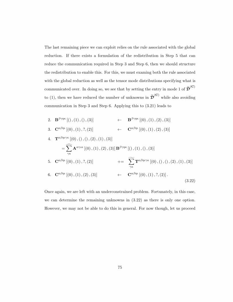
The last remaining piece we can exploit relies on the rule associated with the global

reduction. If there exists a formulation of the redistribution in Step 5 that can

reduce the communication required in Step 3 and Step 6, then we should structure

the redistribution to enable this. For this, we must examing both the rule associated

with the global reduction as well as the tensor mode distributions specifying what is

communicated over. In doing so, we see that by setting the entry in mode 1 of D(C)

to (1), then we have reduced the number of unknowns in D(C)

while also avoiding

communication in Step 3 and Step 6. Applying this to (3.21) leads to

2. Bβγηκ [() , (1) , () , (3)] ← Bβγηκ [(0) , (1) , (2) , (3)]

3. Cαβηι [(0) , (1) , ?, (2)] ← Cαβηι [(0) , (1) , (2) , (3)]

4. Tαβηιγκ [(0) , () , () , (2) , (1) , (3)]

=∑γκ

Aαγικ [(0) , (1) , (2) , (3)] Bβγηκ [() , (1) , () , (3)]

5. Cαβηι [(0) , (1) , ?, (2)] +=∑γκ

Tαβηιγκ [(0) , () , () , (2) , (1) , (3)]

6. Cαβηι [(0) , (1) , (2) , (3)] ← Cαβηι [(0) , (1) , ?, (2)] .

(3.22)

Once again, we are left with an underconstrained problem. Fortunately, in this case,

we can determine the remaining unknowns in (3.22) as there is only one option.

However, we may not be able to do this in general. For now though, let us proceed

75

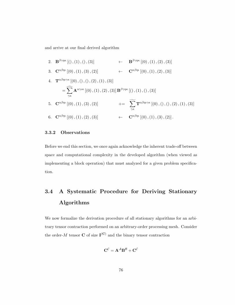
and arrive at our final derived algorithm

2. Bβγηκ [() , (1) , () , (3)] ← Bβγηκ [(0) , (1) , (2) , (3)]

3. Cαβηι [(0) , (1) , (3) , (2)] ← Cαβηι [(0) , (1) , (2) , (3)]

4. Tαβηιγκ [(0) , () , () , (2) , (1) , (3)]

=∑γκ

Aαγικ [(0) , (1) , (2) , (3)] Bβγηκ [() , (1) , () , (3)]

5. Cαβηι [(0) , (1) , (3) , (2)] +=∑γκ

Tαβηιγκ [(0) , () , () , (2) , (1) , (3)]

6. Cαβηι [(0) , (1) , (2) , (3)] ← Cαβηι [(0) , (1) , (3) , (2)] .

3.3.2 Observations

Before we end this section, we once again acknowledge the inherent trade-off between

space and computational complexity in the developed algorithm (when viewed as

implementing a block operation) that must analyzed for a given problem specifica-

tion.

3.4 A Systematic Procedure for Deriving Stationary

Algorithms

We now formalize the derivation procedure of all stationary algorithms for an arbi-

trary tensor contraction performed on an arbitrary-order processing mesh. Consider

the order-M tensor C of size I(C) and the binary tensor contraction

CC = AABB + CC

76

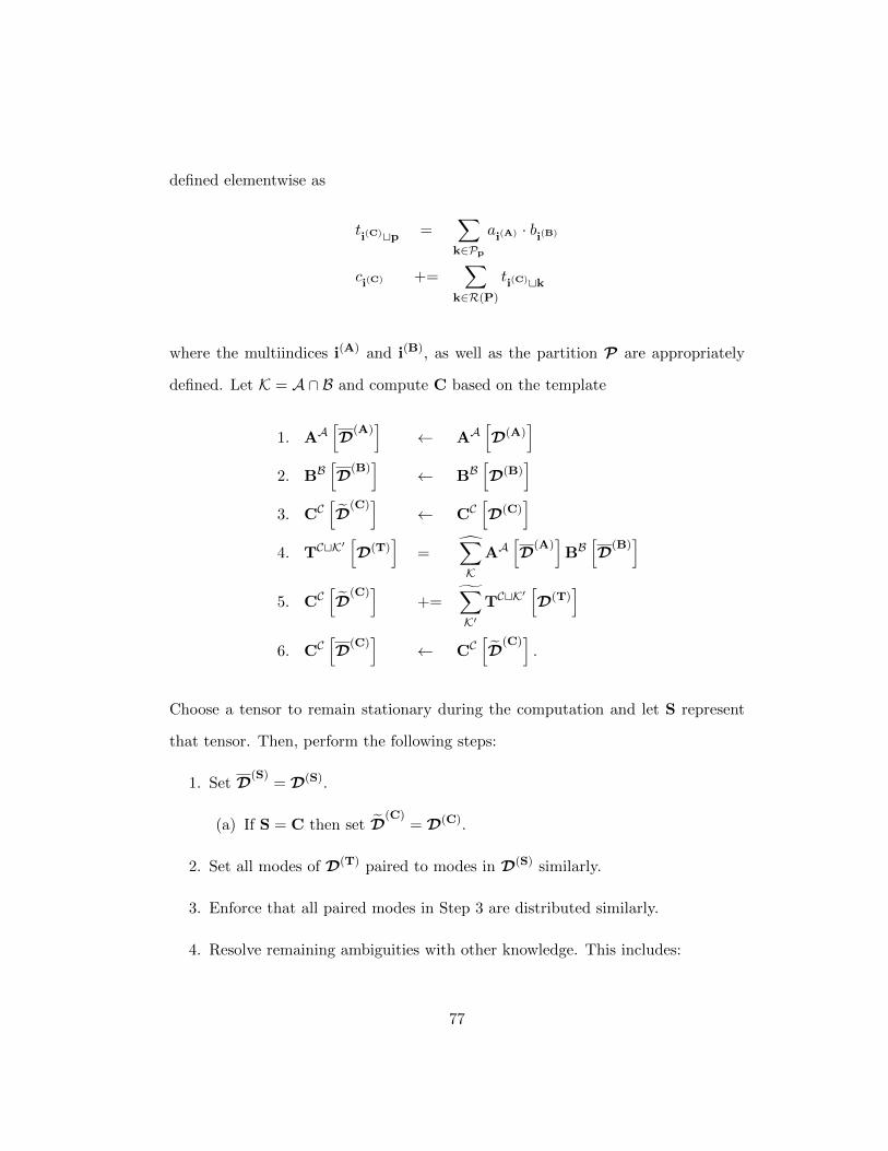
defined elementwise as

ti(C)tp =∑k∈Pp

ai(A) · bi(B)

ci(C) +=∑

k∈R(P)

ti(C)tk

where the multiindices i(A) and i(B), as well as the partition P are appropriately

defined. Let K = A ∩ B and compute C based on the template

1. AA[D(A)

]← AA

[D(A)

]2. BB

[D(B)

]← BB

[D(B)

]3. CC

[D

(C)]

← CC[D(C)

]4. TCtK

′[D(T)

]=

∑K

AA[D(A)

]BB[D(B)

]5. CC

[D

(C)]

+=∑K′

TCtK′[D(T)

]6. CC

[D(C)

]← CC

[D

(C)].

Choose a tensor to remain stationary during the computation and let S represent

that tensor. Then, perform the following steps:

1. Set D(S)= D(S).

(a) If S = C then set D(C)

= D(C).

2. Set all modes of D(T) paired to modes in D(S) similarly.

3. Enforce that all paired modes in Step 3 are distributed similarly.

4. Resolve remaining ambiguities with other knowledge. This includes:

77

(a) If S 6= C then set all nonconflicting entries of D(C)

based on D(C), D(C),

and D(T).

5. Remove any unnecessary steps.

The result of this procedure is an algorithm that performs the desired computation.

A post-processing step that blocks the derived algorithm can then be applied to

reduce the storage requirement of the resulting computations (at the expense of

additional latency in the computation). In Section 3.2.2, we discuss how to select

the correct modes to block.

3.5 Summary

In this chapter, we have shown how the notation proposed in Chapter 2 facilitates

goal-oriented programming [24] for developing parallel algorithms of the tensor con-

traction operation. The direct benefit is that (human or mechanical) experts, tasked

with implementing applications, can significantly reduce the time devoted to opti-

mizing the developed implementations.

One additional benefit of the developed systematic derivation procedure is that

optimizing a series of tensor contractions becomes a (relatively) straightforward ex-

tension of the ideas discussed in this chapter. In particular, recall that we do not

require the initial or final distributions of any object to be specifically set; we only

chose convenient distributions for discussion purposes. As such, optimizing a series

of tensor contractions can be performed by optimizing each contraction separately

and then optimizing the communications that occur between contractions. Perform-

ing this kind of optimization is facilitated by a well-defined notation.

78

Chapter 4

Optimizing Data Movement

In the previous chapter, we discussed how to derive parallel algorithms for the

tensor contraction operation involving dense non-symmetric tensors. One result of

this procedure is that the required data distributions for each step are specified.

In effect, this specifies where data should be moved at each step, but does not

specify how the data should be moved to efficiently redistribute the data. We

would like a method that systematically decomposes an arbitrary specification of a

redistribution into a series of redistributions that rely on balanced communications

as balanced communications can more easily utilize the underlying communication

network effectively.

In addition to this data movement that occurs globally among processes, there are

data movements that occur within processes. Specifically, because we are imple-

menting local tensor contractions in terms of matrix-matrix multiplication, there is

data movement that occurs not only from the beginning or ending of a redistribution

(“packing” and “unpacking”), but that also must be performed in order to correctly

79

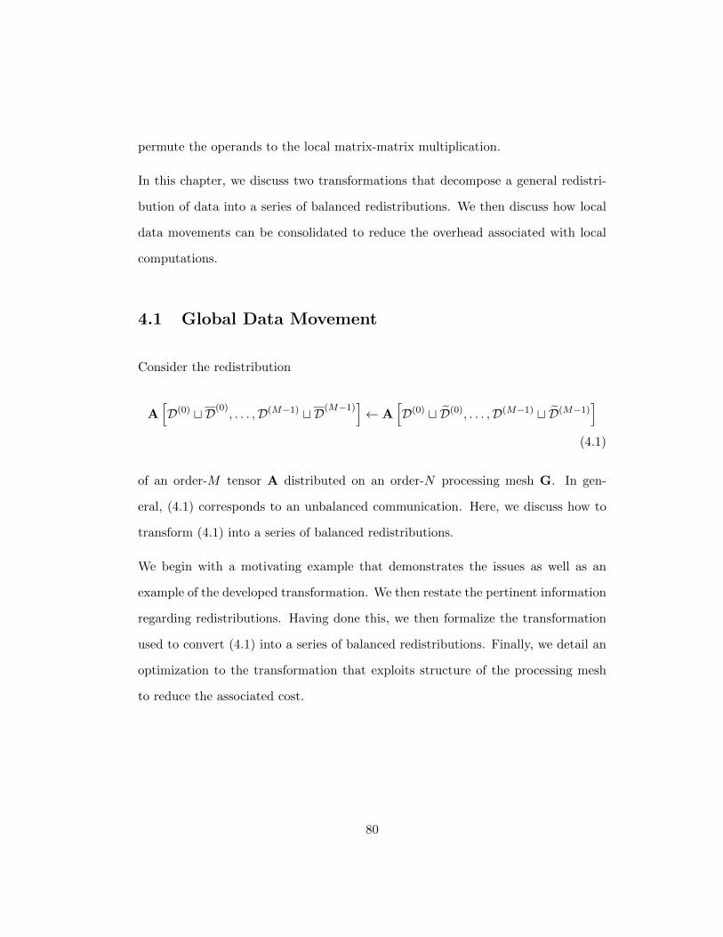
permute the operands to the local matrix-matrix multiplication.

In this chapter, we discuss two transformations that decompose a general redistri-

bution of data into a series of balanced redistributions. We then discuss how local

data movements can be consolidated to reduce the overhead associated with local

computations.

4.1 Global Data Movement

Consider the redistribution

A[D(0) t D(0)

, . . . ,D(M−1) t D(M−1)]← A

[D(0) t D(0), . . . ,D(M−1) t D(M−1)

](4.1)

of an order-M tensor A distributed on an order-N processing mesh G. In gen-

eral, (4.1) corresponds to an unbalanced communication. Here, we discuss how to

transform (4.1) into a series of balanced redistributions.

We begin with a motivating example that demonstrates the issues as well as an

example of the developed transformation. We then restate the pertinent information

regarding redistributions. Having done this, we then formalize the transformation

used to convert (4.1) into a series of balanced redistributions. Finally, we detail an

optimization to the transformation that exploits structure of the processing mesh

to reduce the associated cost.

80

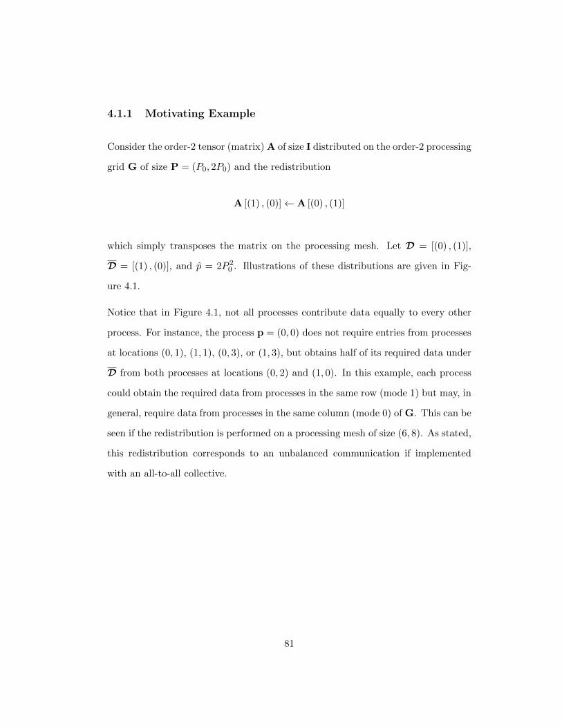
4.1.1 Motivating Example

Consider the order-2 tensor (matrix) A of size I distributed on the order-2 processing

grid G of size P = (P0, 2P0) and the redistribution

A [(1) , (0)]← A [(0) , (1)]

which simply transposes the matrix on the processing mesh. Let D = [(0) , (1)],

D = [(1) , (0)], and p = 2P 20 . Illustrations of these distributions are given in Fig-

ure 4.1.

Notice that in Figure 4.1, not all processes contribute data equally to every other

process. For instance, the process p = (0, 0) does not require entries from processes

at locations (0, 1), (1, 1), (0, 3), or (1, 3), but obtains half of its required data under

D from both processes at locations (0, 2) and (1, 0). In this example, each process

could obtain the required data from processes in the same row (mode 1) but may, in

general, require data from processes in the same column (mode 0) of G. This can be

seen if the redistribution is performed on a processing mesh of size (6, 8). As stated,

this redistribution corresponds to an unbalanced communication if implemented

with an all-to-all collective.

81

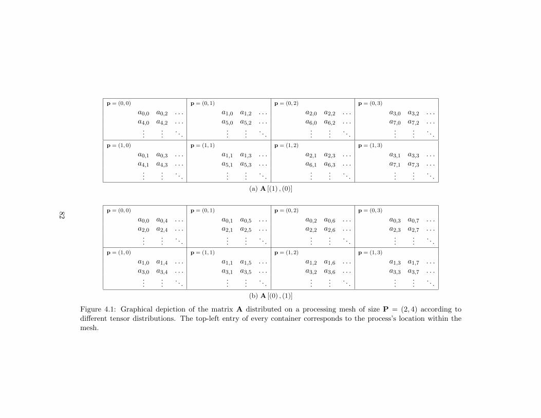
p = (0, 0) p = (0, 1) p = (0, 2) p = (0, 3)

a0,0 a0,2 . . . a1,0 a1,2 . . . a2,0 a2,2 . . . a3,0 a3,2 . . .a4,0 a4,2 . . . a5,0 a5,2 . . . a6,0 a6,2 . . . a7,0 a7,2 . . ....

.... . .

......

. . ....

.... . .

......

. . .

p = (1, 0) p = (1, 1) p = (1, 2) p = (1, 3)

a0,1 a0,3 . . . a1,1 a1,3 . . . a2,1 a2,3 . . . a3,1 a3,3 . . .a4,1 a4,3 . . . a5,1 a5,3 . . . a6,1 a6,3 . . . a7,1 a7,3 . . ....

.... . .

......

. . ....

.... . .

......

. . .

(a) A [(1) , (0)]

p = (0, 0) p = (0, 1) p = (0, 2) p = (0, 3)

a0,0 a0,4 . . . a0,1 a0,5 . . . a0,2 a0,6 . . . a0,3 a0,7 . . .a2,0 a2,4 . . . a2,1 a2,5 . . . a2,2 a2,6 . . . a2,3 a2,7 . . ....

.... . .

......

. . ....

.... . .

......

. . .

p = (1, 0) p = (1, 1) p = (1, 2) p = (1, 3)

a1,0 a1,4 . . . a1,1 a1,5 . . . a1,2 a1,6 . . . a1,3 a1,7 . . .a3,0 a3,4 . . . a3,1 a3,5 . . . a3,2 a3,6 . . . a3,3 a3,7 . . ....

.... . .

......

. . ....

.... . .

......

. . .

(b) A [(0) , (1)]

Figure 4.1: Graphical depiction of the matrix A distributed on a processing mesh of size P = (2, 4) according todifferent tensor distributions. The top-left entry of every container corresponds to the process’s location within themesh.

82

Instead of directly implementing the redistribution based on unbalanced all-to-all

collectives, let us analyze the following series of redistributions that implement the

same overall redistribution:

A [(0) , (1)]

↓ 1. All-to-all over mode 1

A [(0, 1) , ()]

↓ 2. Permutation over modes 0 and 1

A [(1, 0) , ()]

↓ 3. All-to-all over mode 0

A [(1) , (0)] .

Using the costs given in Figure 2.7 and recognizing that now the individual col-

lectives are balanced, the above series of redistributions have an associated cost

of

log2 (2P0)α+ (2P0 − 1)n

2P0β

+ α+ nβ

+ log2 (P0)α+ (P0 − 1)n

P0β

= (1 + log2(2P 2

0

))α+

((2P0 − 1)

2P0+

(P0 − 1)

P0+ 1

)nβ

≈ log2 (p)α+ 3nβ,

which is within a factor 3 of the cost associated with a balanced all-to-all redistri-

bution over p processes.

In the following subsections, we generalize the technique used for the above example

and formalize the transformation to apply to the more general redistribution in

(4.1).

83

4.1.2 Preliminaries

A redistribution is a transformation on a tensor distributions that can perform the

following transformations: reorder entries of tensor mode distributions and trans-

fer entries of a tensor mode distributions to other tensor mode distributions. For

instance, consider the redistribution

A [(2, 0) , (1, 3)]← A [(3, 1, 2) , (0)] .

This redistribution transfers the entries, or processing mesh modes, “1” and “3”

from the mode-0 distribution to the mode-1 distribution and exchanges their order.

Additionally, this redistribution transfers the entry “0” to the mode-0 distribution

and changes the relative ordering of the entries “1”, “2”, and “3”.

In the following two subsections, we discuss how to implement redistributions of the

form

A[D(0) t D(0)

, . . . ,D(M−1) t D(M−1)]← A

[D(0) t D(0), . . . ,D(M−1) t D(M−1)

]

as a series of balanced all-to-all and permutation redistributions. We relate the

effect on data distribution of each balanced redistribution using this interpretation

of redistributions.

For reference, from Figure 2.14, the rule associated with a balanced permutation

redistributions communicating over modes D =⋃

u∈R(M)

D(u) =⋃

u∈R(M)

D(u)is of the

84

form

A[D(0) t D(0), . . . ,D(M−1) t D(M−1)

]↓

A[D(0) t D(0)

, . . . ,D(M−1) t D(M−1)]

where we require that prod(D(u),P

)= prod

(D(u)

,P)

. In other words, we require

that the number of processes used to distribute along modes D(u) is the same as

those used to distribute along modes D(u). The constraint that

⋃u∈R(M)

D(u) =⋃u∈R(M)

D(u)ensures that all entries that exist before the redistribution also exist

after the redistribution. Using Figure 2.7, the associated cost with this redistribution

is

α+ nβ,

where n corresponds to the total number of elements assigned to a process under

the output distribution.

From Figure 2.15, the rule associated with balanced all-to-all redistributions is of

the form

A[D(0), . . . ,D(v−1),D(v) t D(0), . . . ,D(M−1) t D(M−1−v)

]↓

A[D(0) t D(0)

, . . . ,D(v−1) t D(v−1),D(v), . . . ,D(M−1)

],

(4.2)

where (v−1) ∈ R (M) and we assume the entries in both the initial and final tensor

distributions have been consistently permuted.

Let us discuss the interpretation of (4.2). First, we see that we have divided the

tensor modes u ∈ R (M) into two sets: the first v modes, and the last M − v

85

modes. The redistribution in (4.2) proceeds by transferring all modes in D from

their respective tensor mode distributions to the end of the first v tensor mode

distributions via some ordering. As an example redistributions of the form

A [(0, 2, 3) , () , ()] ← A [(0) , (2) , (3)] (v = 1)

A [(0, 3) , (1, 2) , ()] ← A [(0) , (1) , (3, 2)] (v = 2)

A [(0, 2) , (1, 3) , (4)] ← A [(0) , (1) , (4, 3, 2)] (v = 2)

that each transfer entries corresponding to mode 2 and mode 3 are all valid redis-

tributions according to (4.2).

Using Figure 2.7, the associated cost with this redistribution is

log2 (p)α+ (p− 1)n

pβ,

where p corresponds to the total number of processes involved in the communica-

tion.

4.1.3 Balancing Redistributions

We now formalize the technique utilized in Section 4.1.1 to apply to more general

redistribution

A[D(0) t D(0)

, . . . ,D(M−1) t D(M−1)]← A

[D(0) t D(0), . . . ,D(M−1) t D(M−1)

](4.3)

where D =⋃

u∈R(M)

D(u) =⋃

u∈R(M)

D(u).

86

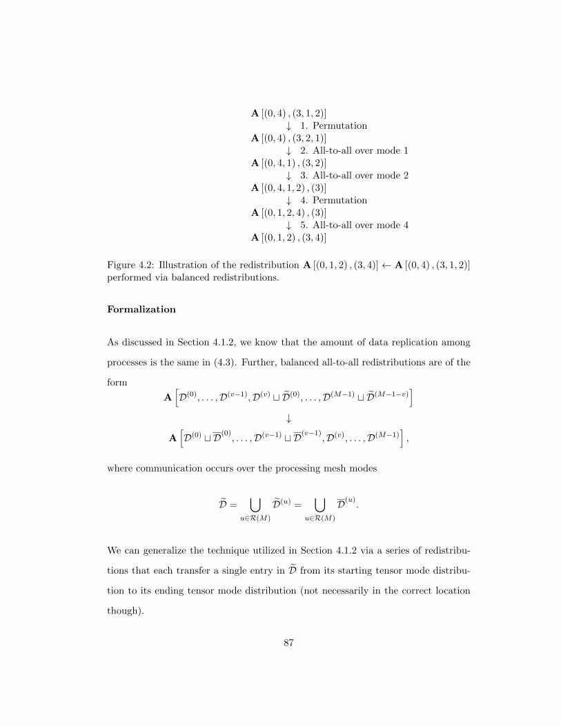
A [(0, 4) , (3, 1, 2)]↓ 1. Permutation

A [(0, 4) , (3, 2, 1)]↓ 2. All-to-all over mode 1

A [(0, 4, 1) , (3, 2)]↓ 3. All-to-all over mode 2

A [(0, 4, 1, 2) , (3)]↓ 4. Permutation

A [(0, 1, 2, 4) , (3)]↓ 5. All-to-all over mode 4

A [(0, 1, 2) , (3, 4)]

Figure 4.2: Illustration of the redistribution A [(0, 1, 2) , (3, 4)]← A [(0, 4) , (3, 1, 2)]performed via balanced redistributions.

Formalization

As discussed in Section 4.1.2, we know that the amount of data replication among

processes is the same in (4.3). Further, balanced all-to-all redistributions are of the

form

A[D(0), . . . ,D(v−1),D(v) t D(0), . . . ,D(M−1) t D(M−1−v)

]↓

A[D(0) t D(0)

, . . . ,D(v−1) t D(v−1),D(v), . . . ,D(M−1)

],

where communication occurs over the processing mesh modes

D =⋃

u∈R(M)

D(u) =⋃

u∈R(M)

D(u).

We can generalize the technique utilized in Section 4.1.2 via a series of redistribu-

tions that each transfer a single entry in D from its starting tensor mode distribu-

tion to its ending tensor mode distribution (not necessarily in the correct location

though).

87

For example, consider the redistribution

A [(0, 1, 2) , (3, 4)]← A [(0, 4) , (3, 1, 2)] .

To transform this redistribution, we can first perform redistributions to move the

entry “1” from the mode-1 distribution to the mode-0 distribution. This requires

a permutation redistribution, followed by an all-to-all redistribution over mode 1.

We can do the same process for the entry “2”, and finally for the entry “4”. A final

permutation redistribution may be required to ensure the entries of each tensor

mode distribution (processing mesh modes) are in the correct order. This results

in the series of redistributions depicted in Figure 4.2. Notice that we perform a

permutation redistribution followed by an all-to-all redistribution over the mode we

are moving.

Thus, (4.3) can be implemented as |D| + 1 permutation redistributions (one last

permutation redistributions to reorder all entries within tensor mode distributions)

and |D| all-to-all redistributions each communicating over a unique entry in D.

To avoid unnecessary complexity in our analyses, we assume that each process is

assigned the same number of elements under the output distribution, denoted n.

If we assume that every mode in R (N) requires this transformation (set R (N) =

88

⋃u∈R(M)

D(u) in (4.3)), then the associated cost is given by

(N + 1) (α+ nβ) +∑

u∈R(N)

(log2 (Pu)α+ (Pu − 1)

n

Puβ

)= (N + 1) (α+ nβ) + log2 (p)α+

∑u∈R(N)

((Pu − 1)

n

Puβ

)≈ (N + 1) (α+ nβ) + log2 (p)α+Nnβ

= (log2 (p) +N + 1)α+ (2N + 1)nβ.

where p = prod(P, D

)is the number of processes involved in an all-to-all collective

instance.

Since we assume that the order of the processing mesh remains constant, the cost of

our transformed redistribution is within a factor 2N + 1 of the cost associated with

a balanced all-to-all collective over the same set of processing mesh modes.

Observations

It is important to mention here that the transformation analyzed represents the

worst case scenario as all processing mesh modes were involved in the communication

and no attempts were made to further optimize redistributions (e.g., merging pairs

of permutation and all-to-all redistributions when possible). This was done for

example purposes only to motivate the idea behind the transformation. Further,

for simplicity we ignored the modes each permutation redistribution communicates

over as this is not reflected in the current cost model used; however, this information

can be tracked if better cost estimates are available.

We now discuss how to reduce the cost associated with the procedure developed in

89

this section by utilizing permutation redistributions to perform some, but preferably

all, of the required transformations on data distribution.

4.1.4 Exploiting Processing Mesh Structure

Once again, we consider the order-M tensor A distributed on the order-N processing

mesh G and the redistribution

A[D(0) t D(0)

, . . . ,D(M−1) t D(M−1)]← A

[D(0) t D(0), . . . ,D(M−1) t D(M−1)

](4.4)

where communication occurs over modes D =⋃

u∈R(M)

D(u) =⋃

u∈R(M)

D(u).

In the previous subsection, we developed a systematic procedure that decomposes

this redistribution into a series of permutation and all-to-all redistributions that has

an associated cost of

(log2 (p) + |D|+ 1

)α+

(2|D|+ 1

)nβ

where p = prod(P, D

)is the number of processes involved in an all-to-all collective

instance and n is the maximum number of elements assigned to a process under the

final distribution.

Notice that if we assume that D(u) = D(u)for all u ∈ R (M), then this redistribu-

tion can be implemented with a single permutation redistribution which results in

a significantly lower associated cost. In general, it is not possible to convert all re-

distributions matching the pattern in (4.4) into a single permutation redistribution,

but we should still attempt to use permutation redistributions whenever possible as

90

the cost associated with the latency term is significantly lower than that associated

with an all-to-all redistribution while having approximately the same cost associated

with the bandwidth term. We now detail a systematic procedure to reduce the cost

associated with the redistribution in (4.4) by utilizing permutation redistributions

whenever possible.

Formalization

Recall that a permutation redistribution has the pattern

A[D(0) t D(0)

, . . . ,D(M−1) t D(M−1)]← A

[D(0) t D(0)

, . . . ,D(M−1) t D(M−1)]

where communication occurs over modes D =⋃

u∈R(M)

D(u) =⋃

u∈R(M)

D(u)and

prod(P, D(u)

)= prod

(P,D(u)

). In other words, the number of processes involved

in a communication over modes D(u) must be the same number as would be involved

if communicating over modes D(u).

Our goal is to determine the entries of D whose transformation can be implemented

via permutation redistributions. In doing so, we identify all entries whose trans-

formation can be directly implemented via permutation redistributions. The trans-

formation associated with the remaining entries then need to be decomposed to be

implemented in terms of balanced redistributions; however, this procedure reduces

the number of entries for which this must be done.

91

To do this, we consider alternative redistributions of the form

A[D(0) tH(0), . . . ,D(M−1) tH(M−1)

]↓

A[D(0) tH(0)

, . . . ,D(M−1) tH(M−1)].

(4.5)

where H(u) ⊆ D(u), H(u) ⊆ D(u), and prod

(P,H(u)

)= prod

(P,H(u)

). Notice

that, as defined, (4.5) corresponds to a balanced permutation redistribution. There-

fore, any definition of H(u) is comprised of entries (processing mesh modes) whose

transformation can be implemented via permutation redistributions. We define J (u)

be the union of all definitions of H(u) and J (u)be the union of all definitions of H(u)

.

We define N (u) = D(u) \ J (u) and N (u)= D(u) \ J (u)

to be the remaining entries.

Finally, we define J =⋃

u∈R(M)

J (u) and N =⋃

u∈R(M)

N (u). We recognize that, in

conjunction with the size of the processing mesh, an analysis of the notation for

the initial and final tensor distributions can determine the definitions of J (u) and

J (u).

We can now decompose the original redistribution in (4.4) into the five steps depicted

in Figure 4.3. Step 1 performs a permutation redistribution that prepares the entries

in J (u) for their transfer from initial tensor mode distribution to final tensor mode

distribution. Step 2 performs a permutation redistribution that transfers the entries

in J (u) to their final tensor mode distributions. Step 3 performs a permutation

redistribution to prepare the entries of N (u) for transferring into their final tensor

mode distribution. Step 4 performs the (potentially unbalanced) redistribution to

transfer the entries of N (u) to their final tensor mode distributions. Finally, Step 5

performs a permutation redistribution to correctly reorder the entries of each tensor

92

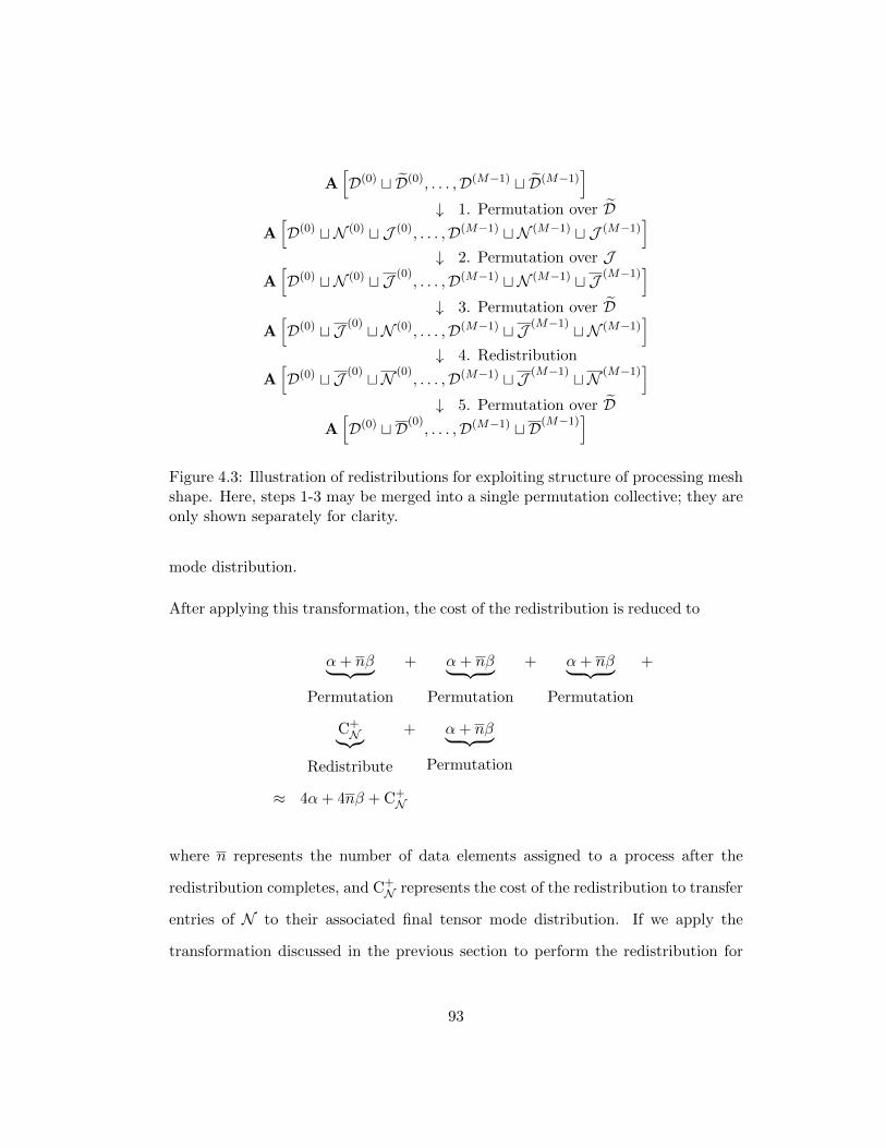
A[D(0) t D(0), . . . ,D(M−1) t D(M−1)

]↓ 1. Permutation over D

A[D(0) tN (0) t J (0), . . . ,D(M−1) tN (M−1) t J (M−1)

]↓ 2. Permutation over J

A[D(0) tN (0) t J (0)

, . . . ,D(M−1) tN (M−1) t J (M−1)]

↓ 3. Permutation over DA[D(0) t J (0) tN (0), . . . ,D(M−1) t J (M−1) tN (M−1)

]↓ 4. Redistribution

A[D(0) t J (0) tN (0)

, . . . ,D(M−1) t J (M−1) tN (M−1)]

↓ 5. Permutation over DA[D(0) t D(0)

, . . . ,D(M−1) t D(M−1)]

Figure 4.3: Illustration of redistributions for exploiting structure of processing meshshape. Here, steps 1-3 may be merged into a single permutation collective; they areonly shown separately for clarity.

mode distribution.

After applying this transformation, the cost of the redistribution is reduced to

α+ nβ︸ ︷︷ ︸Permutation

+ α+ nβ︸ ︷︷ ︸Permutation

+ α+ nβ︸ ︷︷ ︸Permutation

+

C+N︸︷︷︸

Redistribute

+ α+ nβ︸ ︷︷ ︸Permutation

≈ 4α+ 4nβ + C+N

where n represents the number of data elements assigned to a process after the

redistribution completes, and C+N represents the cost of the redistribution to transfer

entries of N to their associated final tensor mode distribution. If we apply the

transformation discussed in the previous section to perform the redistribution for

93

modes N , then we can reduce the estimated cost of

(log2 (p) + |D|+ 1

)α+

(2|D|+ 1

)nβ

where p = prod(P, D

)to

4α+ 4nβ + C+N

≈ 4α+ 4nβ + (log2 (prod (N ,P)) + |N |+ 1)α+ (2|N |+ 1)nβ

= (log2 (prod (N ,P)) + |N |+ 5)α+ (2|N |+ 5)nβ.

We see that the transformation discussed in this section can significantly reduce the

cost associated with the latency term of the redistribution while keeping the cost

associated with the bandwidth term approximately the same.

Observations

A general optimization that can significantly reduce the associated cost of a com-

munication by exploiting the structure of the processing mesh can be described

and reasoned about with the developed notation. Being able to describe how to

systematically decompose these general redistributions into a series of balanced re-

distributions is another example of the utility provided by the developed notation.

Stated another way, the developed notation is powerful enough to capture the per-

tinent knowledge to perform important optimizations while exposing a mechanical

procedure to perform such optimizations.

94

4.2 Local Data Movement

In this section, we discuss how local data movements arising from redistributions and

local computations can be consolidated together, thereby reducing the associated

cost. We focus on the computation of local tensor contractions.

4.2.1 Motivating Example

In Chapter 3, we showed how we derive algorithms for distributed tensor contrac-

tions. An examination of the algorithms derived reveals a common pattern. Each

algorithm follows the steps

1. Globally redistribute tensor operands.

2. Perform local tensor contraction.

3. Globally reduce and/or redistribute tensor operands (if necessary).

A common method of performing the local tensor contraction is to express the

tensor contraction as a matrix-matrix multiplication for which high-performance

implementations exist as part of the BLAS interface [1, 28, 29, 40, 88]. To use

this approach, one must, in the general case, rearrange the data of each tensor.

Assuming we are accumulating into the output operand, this results in potentially

performing four memory rearrangements: three to prepare each of the three tensor

contraction operands for the matrix-matrix multiplication, and one to arrange the

result of the matrix multiplication as specified by the tensor contraction [45]. For

instance, consider the tensor contraction

Cαβηι = AαγικBβγηκ,

95

where we assume a generalized column-major storage for each tensor; that is, indices

of mode 0 are stored contiguously in memory, followed by mode 1, etc. Of course,

there are many possible generalizations of this storage format as we could select

any order of indices to store contiguously. This is similar to how row-major storage

of a matrix column-major storage with the modes interchanged. To express this

computation in terms of matrix-matrix multiplication, we first rearrange the tensors

as

1. Aαιγκ ← Aαγικ.

2. Bγκβη ← Bγκβη.

3. Cαιβη ← Cαβηι.

Then, we recognize that since the indices of the mode pairs (α, ι), (γ, κ), and (β, η)

are stored contiguously in memory, one can view these objects as matrices stored

in column-major order allowing a general matrix-matrix multiplication to perform

the computation. More precisely, the indices of the mode pair (α, ι) correspond

to the “m” dimension, the indices of the mode pair (γ, κ) correspond to the “k”

dimension, and the indices of the mode pair (β, η) correspond to the “n” dimension

of a matrix-matrix multiplication. However, as the output data may not be stored

in the expected order for C, we require one last rearrangement of data to place

elements of C in the correct order.

Expanding our pattern for distributed computations using the knowledge of how lo-

cal tensor contractions are implemented results in the following series of steps

1. Globally redistribute tensor operands.

2. Rearrange local tensor data.

96

3. Perform tensor contraction as matrix-matrix multiplication.

4. Rearrange local tensor data (if necessary).

5. Globally reduce and/or redistribute tensor operands (if necessary).

Now, we also know that performing a redistribution via a collective communication

proceeds according to the following series of steps

(a) Copy data to a send buffer.

(b) Perform communication of data over network storing receiving data in a receive

buffer.

(c) Unpack receive buffer into local storage.

Expanding our distribute algorithm pattern with this knowledge, we arrive at the

following flow for our overall computation

1. (a) Copy data to a send buffer.

(b) Communicate data over the network.

(c) Unpack receive buffer.

2. Rearrange tensor data.

3. Perform matrix-matrix multiplication.

4. Rearrange tensor data (if necessary).

5. (a) Copy data to a send buffer (if necessary).

(b) Communicate data over the network (if necessary).

(c) Unpack receive buffer (if necessary).

97

Notice that the packing/unpacking of communication buffers and the rearrangement

of tensor data both correspond to memory rearrangements. By merging these into

a single rearrangement of data, the overhead associated with these steps is reduced.

As we discussed previously, the only information needed is the order of tensor mode

indices. In doing so, we arrive at our final algorithm template

1. (a) Copy data to a send buffer.

(b) Communicate data over the network.

2. Unpack receive buffer and rearrange tensor data in one step.

3. Perform matrix-matrix multiplication.

4. Rearrange and pack tensor data in one step (if necessary).

5. (a) Communicate data over the network (if necessary).

(b) Unpack receive buffer (if necessary).

Notice that we have roughly halved the number of memory copies required to prepare

a single tensor for local computation. Because this happens at least once for each

tensor, this change removes a large number of unnecessary memory copies.

4.2.2 Generalization

By extending the notation slightly, we can describe how data of each process is

locally stored. With this additional knowledge, an expert can optimize unnecessary

local data movements, thereby increasing the local performance. We do not detail

the extension of the defined notation to incorporate this information as it is not

interesting from a theoretical standpoint.

98

4.3 Summary

In this chapter, we discussed ways to consolidate data movements, both global

movements among processes and local movements within processes, associated with

parallel tensor contraction algorithms and implementations to improve performance.

We discussed two transformations that implement a general redistribution as a series

of balanced redistributions, the second of which reduces the cost of the first trans-

formation by exploiting the structure of the processing mesh. Then, we discussed a

transformation that consolidated memory movements associated with redistribution

and local computation by noticing that the results of both memory movements are

permutations on the data.

We stress here the utility obtained from having developed a notation to describe data

distribution and redistribution. Not only does the developed notation enable exist-

ing transformations to be concisely described, but the notation also facilitates the

generalization of such transformations. For instance, a special case of the optimiza-

tion discussed in Section 4.1.4 is utilized in the distributed-memory tensor library

CTF and the distributed-memory linear algebra libraries Elemental and ScaLA-

PACK. When restricted to matrices, a special case of the same optimization is used

for computing certain linear algebra operations, such as the tridiagonalization of a

symmetric matrix via Householder transformations [33].

In particular, both optimizations discussed in Section 4.1.4 convert the encountered

redistribution into a single permutation redistribution. Section 4.1.4 detailed a pro-

cedure that generalizes this idea to arbitrary redistributions, detecting and applying

the optimization through intermediate redistributions. In doing so, an optimization

whose application choice was binary, now becomes a spectrum of possibilities.

99

Chapter 5

Implementation and

Experimental Results

Previous chapters of this document focused on formalizing different aspects of the

development of high-performance distributed-memory implementations for tensor

contractions. As we saw in Chapter 3 and Chapter 4, there still may exist places

where choices must be made; i.e., the derivation procedure is not entirely systematic.

The space of implementations created by these choices can rapidly become too large

to be reasonably explored even by an expert. In this chapter, we demonstrate how

the ideas presented previously can be translated into a domain-specific language

that can be used by prior work in software engineering for efficiently generating

the optimal implementation among a space of implementations1 for applications of

considerable importance to the domain of computational chemistry.

We begin this chapter by first briefly discussing the application used to test the

1When we refer to optimal, we mean optimal according to the underlying model of computation

100

ideas developed in this document: the spin-adapted CCSD method from compu-

tational chemistry. We then discuss the ROTE library that implements the ideas

associated with data distribution and redistribution as an application programming

interface (API). Next, we discuss some of the ideas behind the software engineering

approach, referred to as Design-by-Transformation (DxT), used to create the space

of implementations for CCSD. As we describe DxT, we relate it to aspects of the

CCSD application and ROTE library for example purposes. Once this is done, we

briefly discuss how the prototype system that implements the ideas of DxT, Dx-

Ter, is used in conjunction with ROTE to generate efficient implementations for the

CCSD application.

We finally move on to discuss experiments used to test the thesis of this dissertation

and provide an analysis of the results. In doing so, we show how the ideas presented

here benefit the state of the art in areas of computer science with potential to

benefit areas of computational chemistry, and provide an argument for approaches

to software development that are based on this clear separation of concerns between

implementation and theoretical aspects of the application domain.

5.1 Coupled Cluster Singles and Doubles

Method (CCSD)

We provide a brief overview of the application used to motivate the ideas in this

dissertation. This section is by no means comprehensive; for a thorough discussion

of CCSD as well as other methods from coupled cluster theory, we recommend [20,

21].

101

5.1.1 Computational Chemistry Background

Quantum mechanical models have proven to be highly accurate for physical sys-

tems. These systems are described by an associated function, called the system’s

wave function. Unfortunately, the exact wave function of a system is typically too

complex to define explicitly. Instead, an approximation to the wave function is used

that maintains useful mathematical properties. The approximated wave function is

typically defined by incorporating models for different physical phenomena into a

reference wave function.

Different methods, referred to as theories, of approximating the true wave function

exist, each having a different associated cost and achieving different levels of accu-

racy [20, 32, 77, 78]. One such theory, known as coupled cluster theory, has been

shown to accurately model chemical systems while retaining desired properties of

the model. In coupled cluster theory, a set of so-called cluster operators are defined

that, when applied to a reference wave function (via the exponential of each cluster

operator), provide an exact representation of the wave function associated with the

system of interest. Each of these operators describe a different instance within a

class of phenomena referred to as excitation. Unfortunately, applying all cluster

operators to construct the true wave function is prohibitively expensive; instead

approximations are made that only apply a subset of the operators defined. A dif-

ferent computational method is then defined by the maximum number of excitations

considered when applying cluster operators.

For instance, the method that accounts for both single and double excitations is

referred to as the “coupled cluster singles and doubles (CCSD)” method [66], while

the method that incorporates single, double, and triple excitations is referred to

102

as the “coupled cluster singles, doubles, and triples (CCSDT)” method [62]. A set

of equations is then derived that defines how to compute associated coefficients for

representing the approximate wave function for the system of interest. Depending

on how the equations are derived, the resulting set of equations can have different

computational characteristics. Further, the derived set of equations may require

exploiting structure such as symmetry within the tensor data. Incorporating sym-

metry is a topic of future research and is not discussed in this thesis.

Beyond limiting the set of cluster operators, further approximations can be made

or techniques can be used to reduce the complexity of the resulting equations or

factorization process. For instance, methods based on perturbation theory can be

applied to approximate certain cluster operators (such as the triples operator) [68].

Spin-adaptation refers to a technique that produces sets of equations that can be

efficiently computed while enforcing certain constraints to accurately model the

system of interest [50, 59, 75].

5.1.2 The Specific Formulation Studied

For the purposes of this dissertation, it suffices to understand that these methods

boil down to a computation involving many tensor contractions where the output

of one tensor contraction may be the input for another and/or the results must

be summed. The specific formulation of the spin-adapted CCSD method studied

in this document is given in Figure 5.1. There, we use the notation familiar to

computational chemists. Focusing on the computation of Gmi in Figure 5.1,

∑e

Hme t

ei

103

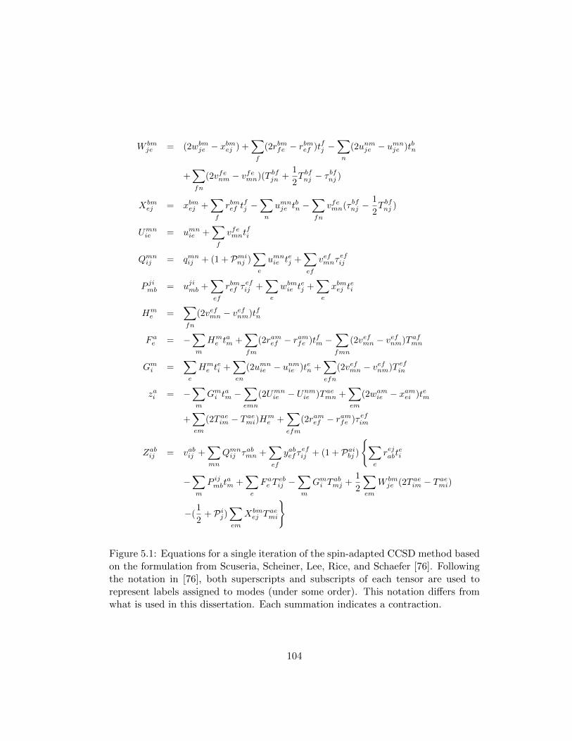
W bmje = (2wbm

je − xbmej ) +∑f

(2rbmfe − rbmef )tfj −∑n

(2unmje − umnje )tbn

+∑fn

(2vfenm − vfemn)(T bfjn +

1

2T bfnj − τ

bfnj )

Xbmej = xbmej +

∑f

rbmef tfj −

∑n

umnje t

bn −

∑fn

vfemn(τ bfnj −1

2T bfnj )

Umnie = umn

ie +∑f

vfemntfi

Qmnij = qmn

ij + (1 + Pminj )

∑e

umnie tej +

∑ef

vefmnτefij

P jimb = ujimb +

∑ef

rbmef τefij +

∑e

wbmie t

ej +

∑e

xbmej tei

Hme =

∑fn

(2vefmn − vefnm)tfn

F ae = −

∑m

Hme t

am +

∑fm

(2ramef − ramfe )tfm −∑fmn

(2vefmn − vefnm)T afmn

Gmi =

∑e

Hme t

ei +

∑en

(2umnie − unmie )ten +

∑efn

(2vefmn − vefnm)T efin

zai = −∑m

Gmi t

am −

∑emn

(2Umnie − Unm

ie )T aemn +

∑em

(2wamie − xamei )tem

+∑em

(2T aeim − T ae

mi)Hme +

∑efm

(2ramef − ramfe )τefim

Zabij = vabij +

∑mn

Qmnij τabmn +

∑ef

yabefτefij + (1 + Pai

bj )

{∑e

rejabtei

−∑m

P ijmbt

am +

∑e

F ae T

ebij −

∑m

Gmi T

abmj +

1

2

∑em

W bmje (2T ae

im − T aemi)

−(1

2+ Pi

j)∑em

Xbmej T

aemi

}

Figure 5.1: Equations for a single iteration of the spin-adapted CCSD method basedon the formulation from Scuseria, Scheiner, Lee, Rice, and Schaefer [76]. Followingthe notation in [76], both superscripts and subscripts of each tensor are used torepresent labels assigned to modes (under some order). This notation differs fromwhat is used in this dissertation. Each summation indicates a contraction.

104

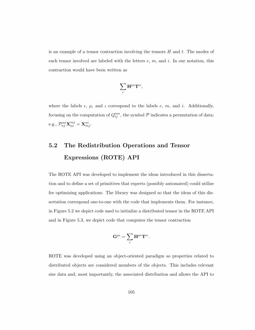
is an example of a tensor contraction involving the tensors H and t. The modes of

each tensor involved are labeled with the letters e, m, and i. In our notation, this

contraction would have been written as

∑ε

HµεTει,

where the labels ε, µ, and ι correspond to the labels e, m, and i. Additionally,

focusing on the computation of Qmnij , the symbol P indicates a permutation of data;

e.g., Pminj Xmjni = Xni

mj .

5.2 The Redistribution Operations and Tensor

Expressions (ROTE) API

The ROTE API was developed to implement the ideas introduced in this disserta-

tion and to define a set of primitives that experts (possibly automated) could utilize

for optimizing applications. The library was designed so that the ideas of this dis-

sertation correspond one-to-one with the code that implements them. For instance,

in Figure 5.2 we depict code used to initialize a distributed tensor in the ROTE API

and in Figure 5.3, we depict code that computes the tensor contraction

Gµι =∑ε

HµεTει.

ROTE was developed using an object-oriented paradigm so properties related to

distributed objects are considered members of the objects. This includes relevant

size data and, most importantly, the associated distribution and allows the API to

105

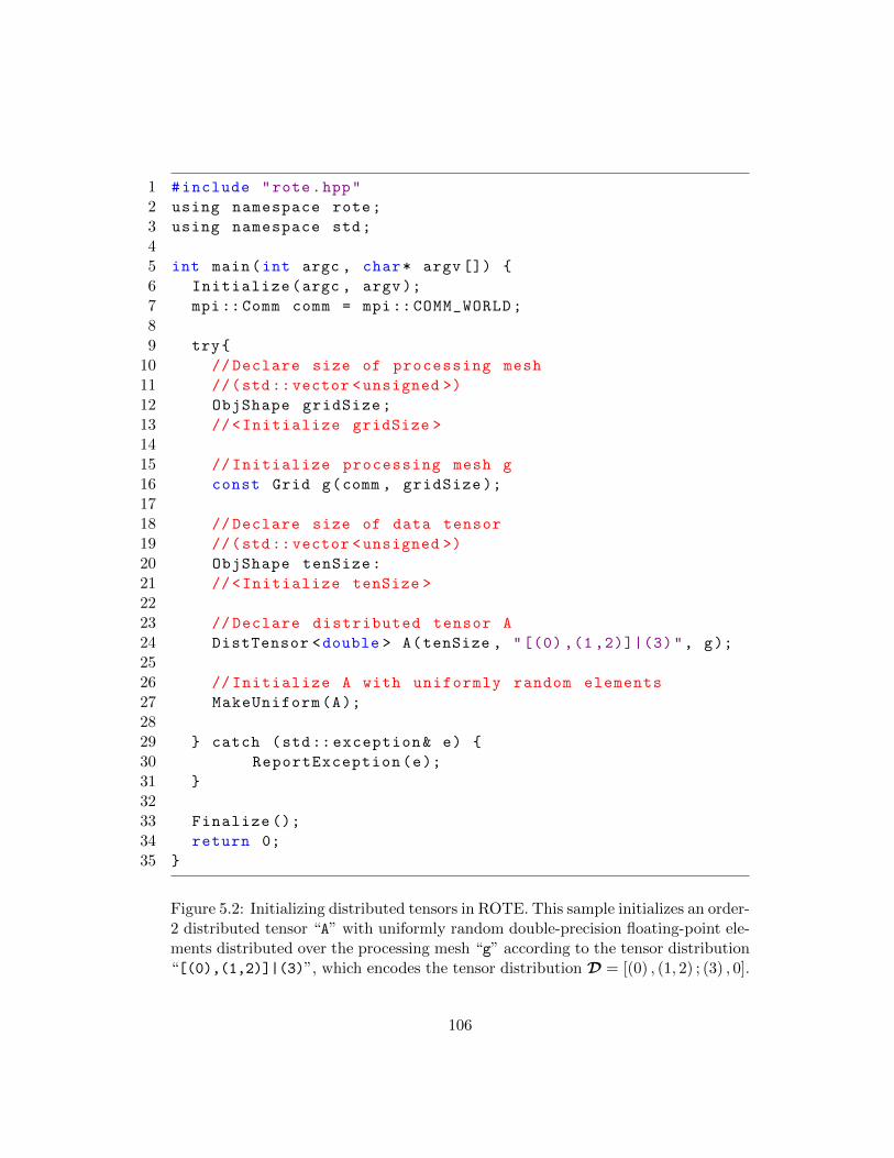
1 #include "rote.hpp"

2 using namespace rote;

3 using namespace std;

45 int main(int argc , char* argv []) {

6 Initialize(argc , argv);

7 mpi::Comm comm = mpi:: COMM_WORLD;

89 try{

10 // Declare size of processing mesh

11 //(std::vector <unsigned >)

12 ObjShape gridSize;

13 //<Initialize gridSize >

1415 // Initialize processing mesh g

16 const Grid g(comm , gridSize );

1718 // Declare size of data tensor

19 //(std::vector <unsigned >)

20 ObjShape tenSize:

21 //<Initialize tenSize >

2223 // Declare distributed tensor A

24 DistTensor <double > A(tenSize , "[(0) ,(1 ,2)]|(3)", g);

2526 // Initialize A with uniformly random elements

27 MakeUniform(A);

2829 } catch (std:: exception& e) {

30 ReportException(e);

31 }

3233 Finalize ();

34 return 0;

35 }

Figure 5.2: Initializing distributed tensors in ROTE. This sample initializes an order-2 distributed tensor “A” with uniformly random double-precision floating-point ele-ments distributed over the processing mesh “g” according to the tensor distribution“[(0),(1,2)]|(3)”, which encodes the tensor distribution D = [(0) , (1, 2) ; (3) , 0].

106

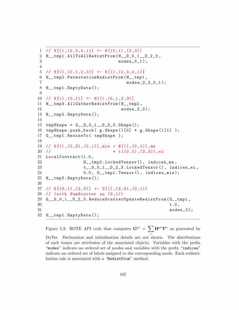
1 // H[(),(2,3,0,1)] <- H[(0 ,1) ,(2 ,3)]

2 H__tmp1.AllToAllRedistFrom(H__D_0_1__D_2_3 ,

3 modes_0_1 );

45 // H[(),(0,1,2,3)] <- H[(),(2,3,0,1)]

6 H__tmp2.PermutationRedistFrom(H__tmp1 ,

7 modes_2_3_0_1 );

8 H__tmp1.EmptyData ();

910 // H[() ,(0 ,1)] <- H[(),(0,1,2,3)]

11 H__tmp3.AllGatherRedistFrom(H__tmp2 ,

12 modes_2_3 );

13 H__tmp2.EmptyData ();

1415 tmpShape = G__D_0_1__D_2_3.Shape ();

16 tmpShape.push_back( g.Shape ()[0] * g.Shape ()[1] );

17 G__tmp1.ResizeTo( tmpShape );

1819 // G[() ,(2 ,3) ,(0 ,1)] _mie = H[() ,(0 ,1)] _me

20 // * t[(0 ,1) ,(2 ,3)] _ei

21 LocalContract (1.0,

22 H__tmp3.LockedTensor (), indices_me ,

23 t__D_0_1__D_2_3.LockedTensor (), indices_ei ,

24 0.0, G__tmp1.Tensor(), indices_mie );

25 H__tmp3.EmptyData ();

2627 // G[(0 ,1) ,(2 ,3)] <- G[() ,(2 ,3) ,(0 ,1)]

28 // (with SumScatter on (0,1))

29 G__D_0_1__D_2_3.ReduceScatterUpdateRedistFrom(G__tmp1 ,

30 1.0,

31 modes_2 );

32 G__tmp1.EmptyData ();

Figure 5.3: ROTE API code that computes Gµι =∑ε

HµεTει as generated by

DxTer. Declaration and initialization details are not shown. The distributionsof each tensor are attributes of the associated objects. Variables with the prefix“modes” indicate an ordered set of modes and variables with the prefix “indices”indicate an ordered set of labels assigned to the corresponding mode. Each redistri-bution rule is associated with a “RedistFrom” method.

107

capture the notation in this dissertation while hiding low level details. As a result,

ROTE becomes a domain-specific language for tensor contractions on distributed

memory architectures.

Redistributions, in terms of the general rules defined in Figure 2.14 and Figure 2.15,

are implemented in the API as sophisticated wrapper routines to underlying MPI

collective communications and local tensor contractions are presently implemented

as a wrapper to a high-performance matrix-matrix multiplication kernel.

5.3 Design-by-Transformation (DxT) and DxTer

Here, we provide a general overview of the DxT approach to software develop-

ment [53, 57] and the prototype system DxTer. We then discuss how DxT and

DxTer is used in the context of this dissertation work. For a detailed discussion of

DxT and DxTer, we encourage the reader to read [58].

5.3.1 Background

The DxT approach to software development is to create application implementa-

tions by converting abstract representations of the application to efficient, concrete

implementations via a series of correct transformations [57]. This process facilitates

the automatic generation of efficient implementations that is ordinarily performed

by a human expert.

We now discuss how this approach is applied to the design of implementations for

CCSD using the functionality defined in the ROTE API as building blocks, or prim-

itives as defined in the DxT terminology. Let us focus on how an implementation

108

for the expression

Gmi =∑e

Hme t

ei +

∑en

(2umnie − unmie )ten +∑efn

(2vefmn − vefnm)T efin

in Figure 5.1 would be created with the DxT approach. We see that G is formed by

the accumulation of three contractions involving five inputs in total (Hme , tei , u

mnie ,

T efin , and vefmn).

First, the computation is encoded as a dataflow graph. Each node in this graph

represents some computation and edges between nodes represent data dependencies

between computations. For example, each term (contraction) would be represented

as a node in the graph, and the data dependencies of each input to the computation

of Gmi (Hme , T efin , vefmn, umnie ) would be represented as edges between different nodes

in the graph. We mention that no details of how each computation should proceed

are defined at this point, only the abstract representations of the computations along

with data dependencies are encoded.

Our end goal is to transform our abstract representation of the computation into a

representation that only relies on concretely defined operations whose implementa-

tions are provided, referred to as primitives. We do this by continually applying a set

of transformation rules, called refinements, to our dataflow graph until all details of

the computation are concrete. Once this is done, we have an implementation for the

original problem statement. For instance, a refinement corresponds to a transfor-

mation that converts a node in our dataflow graph representing a tensor contraction

into one representing a stationary variant of the algorithm; we have not yet arrived

at a implementation as not all details have been filled in (such as how the necessary

109

redistributions are performed)2. Examples of primitives are the implementations

provided by the ROTE API of each redistribution rule given in Figures 2.14 and

2.15.

Having defined computations (as dataflow graphs), refinements, and an associated

set of primitives, we are able to transform our abstract representation into a concrete

implementation. Depending on the order that we apply our refinements, we can

arrive at different implementations. Therefore, our set of refinements and primitives

define a space of implementations for our algorithm. Of course, we would like

to ensure that some of the produced implementations are efficient. For this, we

associate a cost with each primitive considered and define transformations on the

dataflow graph that, upon application, result in a dataflow graph with better overall

cost. These transformations are referred to as optimizations. For example, the

transformations described in Chapter 4 to convert general redistributions into a

series that rely on balanced communications are optimizations as they reduce the

cost associated with the bandwidth term of the communications.

At this point, we have a way to create a space of implementations for an application

that is based on a systematic process and a way to rank order each implementation.

The task of creating an efficient implementation for a specific computation has been

reduced to one of searching within a space of implementations. The prototype

system DxTer, created by Bryan Marker as part of his dissertation work, was used

to implement the ideas of DxT discussed in this section and efficiently search the

space of implementations for the optimal [55, 58].

2Strictly speaking, refinements are not required to provide more concrete details, but this detaildoes not add to the discussion.

110

5.3.2 DxT and This Dissertation

In the context of this dissertation, DxTer used the methods defined in ROTE as

primitives to generate efficient implementations for the CCSD application. Due

to the generality of the ideas developed in this document, the encoded rules allow

DxTer to consider implementations for a particular arrangement of processes, a

contribution that is of great importance since, for certain architectures such as

the tested Blue Gene/Q architecture, the exact arrangement of processes (called a

partition on that architecture) is made available to the user and can be exploited in

the optimization.

At this point we cannot guarantee that the generated implementations are optimal

for the experimental setup. We simply rely on DxTer to generate implementations

that are reasonable in terms of the choices made for algorithmic variants and compo-

sition of redistribution rules. In encoding the rules for implementation, the expert

should refine the rules so that DxTer can find an efficient solution using the en-

coded knowledge (this corresponds either to cost adjustments or additions to the

encoded knowledge). Note that this process requires significant work by an expert

to encode and refine the rules; however, once done, DxTer can be used to generate

implementations for all applications relying on the encoded knowledge. Addition-

ally, the implementations developed using DxTer and ROTE were post-processed to

add blocking so that the problems being computed could mitigate the effect of extra

storage required for data replication. This enabled larger problems to be solved and

potentially achieve better overall performance, as discussed in Section 5.4.4.

111

5.4 Experimental Results

We now turn to results of computing the spin-adapted CCSD method on massively-

parallel distributed-memory architectures. The ideas of this dissertation directly

apply to this application as the computations involved are a series of dense, non-

symmetric, tensor contractions. Implementations were generated assuming a spec-

ified order-4 processing mesh and sizes for tensors that represent real-world appli-

cations of CCSD. For those familiar with the method, this corresponds to problem

specifications where the number of virtual orbitals is an order of magnitude greater

than the number of occupied orbitals.

5.4.1 Target Architectures

Experiments were conducted on the IBM Blue Gene/Q [83] and Cray XC30 [22]

computing architectures, comparing against two other widely used packages for

performing distributed-memory parallel tensor computations: the Cyclops Tensor

Framework (CTF)3 and the CCSD module in the NorthWest computational Chem-

istry (NWChem) software package [14]. Details of CTF and the related module in

NWChem are given in Chapter 6. Implementations were created in CTF that rep-

resent the same set of equations computed by implementations generated by DxTer

with ROTE. As NWChem is not properly tuned for the IBM Blue Gene/Q archi-

tecture, we only compare against NWChem on the Cray XC30 architecture.

For the IBM Blue Gene/Q architecture, compute nodes consist of sixteen 1600MHz

PowerPC A2 cores for a combined theoretical peak performance of 204.8 GFlops per

node using double-precision arithmetic. Nodes are connected via a five-dimensional

3The version of CTF used was dated Feb. 5, 2015.

112

torus topology that supports a chip-to-chip bandwidth of 2GB/s.

For the Cray XC30 architecture, compute nodes consist of twelve 2400MHz Intel

“Sandybridge” cores for a combined theoretical peak of 460.8 GFlops per node

using double-precision arithmetic. In this case, nodes are connected via a Cray

Aries interconnect with DragonFly topology [43] supporting a global bandwidth of

23.7 TB/s.

When possible, experiments were performed using the same parameters for compiler

optimization, underlying BLAS library, and MPI implementation (multithreaded

ESSL on Blue Gene/Q and multithreaded MKL on Cray XC30). For a fair compar-

ison, tuning parameters for each set of implementations were adjusted and values

associated with the best performance results were reported. For CTF, ROTE, and

NWChem, these include a form of on-node configuration; however, in the case of

ROTE, the additional parameter of the processing mesh used to generate implemen-

tations was tested.

We mention here one important aspect of the results for the ROTE-based imple-

mentations. For computational chemists, a sought-after property of any distributed-

memory tensor library is that high performance is achieved when fifty percent of

the available memory is reserved for inputs. As we see in the following sections, our

implementations achieve this.

5.4.2 IBM Blue Gene/Q Experiments

Comparison with CTF. In Figure 5.4, we show experimental results comparing

ROTE-based implementations against implementations created in CTF using 32

nodes (512 cores) and 512 nodes (8192 cores). In each of these experiments, we

113

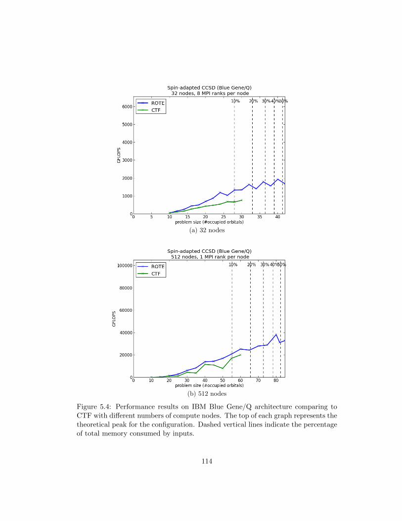
(a) 32 nodes

(b) 512 nodes

Figure 5.4: Performance results on IBM Blue Gene/Q architecture comparing toCTF with different numbers of compute nodes. The top of each graph represents thetheoretical peak for the configuration. Dashed vertical lines indicate the percentageof total memory consumed by inputs.

114

plot raw performance achieved by each implementation as the associated problem

size is increased (in terms of the number of occupied orbitals represented in the

computation). The top of each graph indicates the maximum performance, or peak,

achievable by the configuration. Each set of implementations were tested until

memory exhaustion; therefore, the final data point shown represents the largest

problem able to be computed with the available resources. Dashed vertical lines are

overlaid on the figures to depict the percentage of total memory required to store

the inputs for the computation with associated problem size.

It can be seen that the ROTE-based implementations outperform CTF. Addi-

tionally, the ROTE-based implementations can perform computations that require

approximately three times the amount of memory for input using the same re-

sources.

In the case of the 32-node experiment, a configuration of eight MPI ranks per

node and eight OpenMP threads per MPI rank achieved the best results for each

library; for the 512-node experiment, a configuration of one MPI rank and sixty four

OpenMP threads per rank achieved the best performance for both libraries. These

configurations correspond to using a processing mesh of size (4, 4, 4, 4) for the 32-

node experiment and a processing mesh of size (2, 4, 8, 8) for the 512-node experiment

for the ROTE library. As mentioned in the previous subsection, we cannot comment

on the processing mesh configuration chosen by CTF as this is handled internally by

the library. However, notice that in the 32-node experiment, all grid modes have the

same dimension meaning that many all-to-all redistributions can be implemented in

terms of permutation redistributions as discussed in Chapter 4.

Interestingly, for the 512-node experiment, a processing mesh of size (2, 4, 8, 8)

achieved the best performance even though a processing mesh configuration of

115

(8, 8, 8, 8) can be created by assigning eight MPI ranks per node and eight OpenMP

threads per rank instead of one MPI rank and sixty four OpenMP threads. The

reason for this is likely due to a trade-off between allgather redistributions and all-to-

all redistributions that occurs in each configuration. In the (8, 8, 8, 8) configuration,

many all-to-all redistributions can be implemented with permutation redistributions,

but the allgather redistributions may involve a greater number of processes than in

the (2, 4, 8, 8) configuration.

Notice that, based on the problem specification, many allgather redistributions oc-

cur on mode 0 and mode 1 of the processing mesh. In the case of the (8, 8, 8, 8)

configuration, this means that up to sixty four processes are involved in the redis-

tributions, whereas in the (2, 4, 8, 8) configuration, only at most eight are. This is

an example of where the trade-off between performance of different transformations

and collective communications must be considered to achieve a higher performing

implementation; in the (2, 4, 8, 8) case, we limit the opportunities to implement

an all-to-all collective as a permutation collective, but reduce the cost of allgather

collectives, whereas the (8, 8, 8, 8) case has the opposite property.

5.4.3 Cray XC30 Experiments

Comparison with CTF. In Figure 5.5, we show performance results comparing

the ROTE-based implementation to the CTF implementation using 32 nodes (768

cores) and 512 nodes (12288 cores) of the Cray XC30 architecture. As with the

experiments performed on the IBM Blue Gene/Q, in each of these experiments, we

plot raw performance achieved by each implementation as the associated problem

size is increased (in terms of the number of occupied orbitals represented in the

computation). The top of each graph indicates the maximum performance, or peak,

116

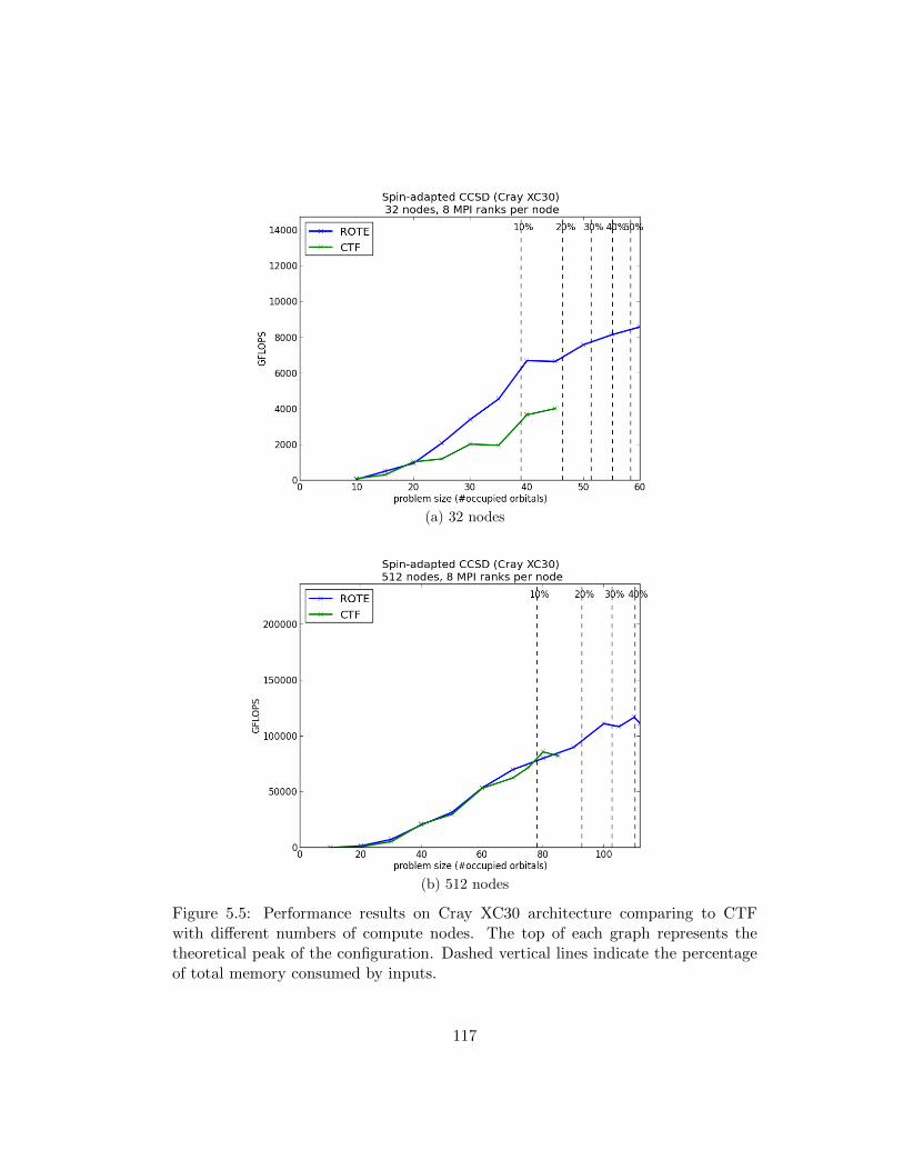
(a) 32 nodes

(b) 512 nodes

Figure 5.5: Performance results on Cray XC30 architecture comparing to CTFwith different numbers of compute nodes. The top of each graph represents thetheoretical peak of the configuration. Dashed vertical lines indicate the percentageof total memory consumed by inputs.

117

achievable by the configuration. Each set of implementations were tested until

memory exhaustion; therefore, the final data point shown represents the largest

problem able to be computed with the available resources. Dashed vertical lines are

overlaid on the figures to depict the percentage of total memory required to store

the inputs for the computation with associated problem size.

A node configuration of eight MPI ranks per node and three OpenMP threads

per MPI rank achieved the best results for both the ROTE-based implementation

and CTF in both the 32-node and 512-node experiments. These configurations

correspond to using a processing mesh of size (4, 4, 4, 4) for the 32-node case and a

processing mesh of size (8, 8, 8, 8) for the 512-node case. We see that the ROTE-

based implementation is able to achieve performance that is at least comparable to

the CTF implementation, but in some cases outperforms CTF.

It is interesting that in this case, the performance of the ROTE-based implemen-

tation does not outperform CTF code as much as on the BG/Q architecture. We

suspect that this is due in part to the relatively faster communication network of the

Cray XC30 architecture that allows differences between communication performance

to be hidden [60, 64].

Comparison with NWChem. In Figure 5.6, we show performance results com-

paring the ROTE-based implementation to the hand-coded implementation pro-

vided in the NWChem package [84] (version 6.3) using 32 nodes (768 cores) and

512 nodes (12288 cores) of the Cray XC30 architecture. When performing these

experiments, an implementation a bug was discovered in more recent NWChem

implementations that potentially hindered the achievable performance. Instead, a

recent stable version of NWChem was used for performance experiments.

118

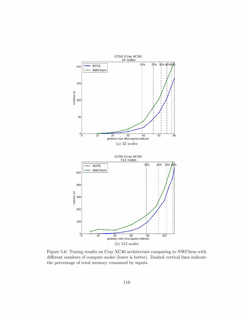
(a) 32 nodes

(b) 512 nodes

Figure 5.6: Timing results on Cray XC30 architecture comparing to NWChem withdifferent numbers of compute nodes (lower is better). Dashed vertical lines indicatethe percentage of total memory consumed by inputs.

119

Although the set of equations implemented in NWChem are chemically equivalent

to those in the ROTE-based implementations, they have different computational

and communication characteristics. Of particular note is the fact that the NWChem

implementation relies on an approach to computing the dominant term of CCSD that

significantly reduces the overall storage requirement. This enables the NWChem

implementation to perform computations that require significantly more storage

for inputs as the ROTE-based implementations cannot exploit the structure of the

computation to obtain this benefit. Therefore, we plot the relative runtimes of each

implementation instead of the raw performance achieved and only show results up to

the largest computation able to be performed by ROTE-based implementations with

the given resources (to conserve computing resources). Here, we also use dashed

vertical lines to indicate the percentage of memory required to store the inputs

associated with different computations.

In the 32-node case, implementations based on a processing mesh of size (4, 4, 4, 4)

achieved the best performance for the ROTE-based implementation, and imple-

mentations based on a processing mesh of size (8, 8, 8, 8) achieved the best in the

512-node case. Considering the assumptions about these experiments, we see that

although the ROTE-based implementations can only solve smaller problems with

the same resources, they are able to outperform the hand-coded implementations

provided by NWChem.

5.4.4 The Importance of Blocking

As mentioned in Section 2.5, blocking the overall computation into a series of sub-

problems can mitigate the effect on storage at the expense of additional communi-

cation overhead; a larger block size requires a larger amount of storage to perform

120

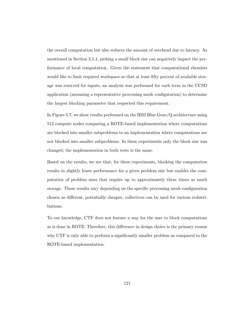
the overall computation but also reduces the amount of overhead due to latency. As

mentioned in Section 2.5.1, picking a small block size can negatively impact the per-

formance of local computation. Given the statement that computational chemists

would like to limit required workspace so that at least fifty percent of available stor-

age was reserved for inputs, an analysis was performed for each term in the CCSD

application (assuming a representative processing mesh configuration) to determine

the largest blocking parameter that respected this requirement.

In Figure 5.7, we show results performed on the IBM Blue Gene/Q architecture using

512 compute nodes comparing a ROTE-based implementation where computations

are blocked into smaller subproblems to an implementation where computations are

not blocked into smaller subproblems. In these experiments only the block size was

changed; the implementation in both tests is the same.

Based on the results, we see that, for these experiments, blocking the computation

results in slightly lower performance for a given problem size but enables the com-

putation of problem sizes that require up to approximately three times as much

storage. These results vary depending on the specific processing mesh configuration

chosen as different, potentially cheaper, collectives can be used for various redistri-

butions.

To our knowledge, CTF does not feature a way for the user to block computations

as is done in ROTE. Therefore, this difference in design choice is the primary reason

why CTF is only able to perform a significantly smaller problem as compared to the

ROTE-based implementation.

121

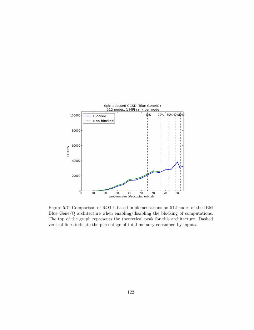
Figure 5.7: Comparison of ROTE-based implementations on 512 nodes of the IBMBlue Gene/Q architecture when enabling/disabling the blocking of computations.The top of the graph represents the theoretical peak for this architecture. Dashedvertical lines indicate the percentage of total memory consumed by inputs.

122

5.4.5 Weak Scalability Experiments

Metrics referred to as scalability are commonly used measure the quality of a par-

allel implementation. The scalability of a parallel implementation refers to how

the implementation performs when additional processing elements are added to the

system.

Strong scalability refers to how the implementation performs when additional pro-

cessing elements are added to the system with the goal of reducing the time re-

quired to perform a computation of fixed size. For this metric, a perfectly scalable

implementation would halve the time required to perform a computation when the

number of processing elements is doubled. Perfect strong scalability is not achiev-

able for problems in this domain. Because the total amount of computation remains

constant while the overhead associated with communication inherently scales with

the number of processes in the system, the efficiency of each processing element

cannot be maintained.

Weak scalability refers to how the implementation performs when additional pro-

cessing elements are added to the system with the goal of maintaining the computing

efficiency. For this metric, a perfectly scalable implementation would maintain the

computing efficiency when the problem size (in terms of memory usage) is scaled in

proportion to the number of processes involved. For example, a perfectly scalable

implementation would maintain the computing efficiency when twice as many pro-

cesses are used to solve a problem requiring twice as much storage for inputs. For

applications in this domain, we are typically concerned with weak scalability.

In Figure 5.8, we show the results of weak scalability experiments of the ROTE-

based implementations up to 512 nodes on both the IBM Blue Gene/Q and Cray

123

XC30 architectures (8192 and 12288 cores respectively). For each configuration

tested, approximately fifty percent of the available storage was reserved for inputs

of the CCSD application thus making memory use per process roughly constant. An

examination of these results reveals that the computing efficiency of each process is

held nearly constant as the number of nodes is increased in the Blue Gene/Q case,

and drops slightly as the number of nodes increases in the Cray XC30 case. This

provides some evidence of relatively good weak scalability in the implementation

used. To prove weak scalability, a cost analysis would have to be performed for the

generated implementation, which is beyond the scope of this dissertation.

We mention here that the implementations chosen for each configuration in this

case are not necessarily the same. We expect that if the same implementation was

chosen for the 32 node case as for the 512 node case, the weak scalability would

worsen as the relationship between processing mesh configuration and collectives

utilized may be less advantageous. Different implementations were chosen for each

configuration to mitigate this effect. This is still a valid measure of scalability,

as our implementation for this domain is to incorporate the configuration of the

processing mesh when developing an implementation for the application (therefore

the implementation being measured is not dependent on any specific implementation

chosen).

124

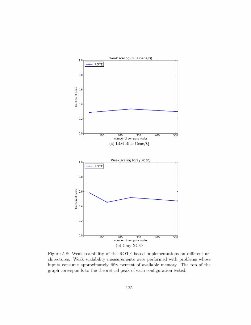
(a) IBM Blue Gene/Q

(b) Cray XC30

Figure 5.8: Weak scalability of the ROTE-based implementations on different ar-chitectures. Weak scalability measurements were performed with problems whoseinputs consume approximately fifty percent of available memory. The top of thegraph corresponds to the theoretical peak of each configuration tested.

125

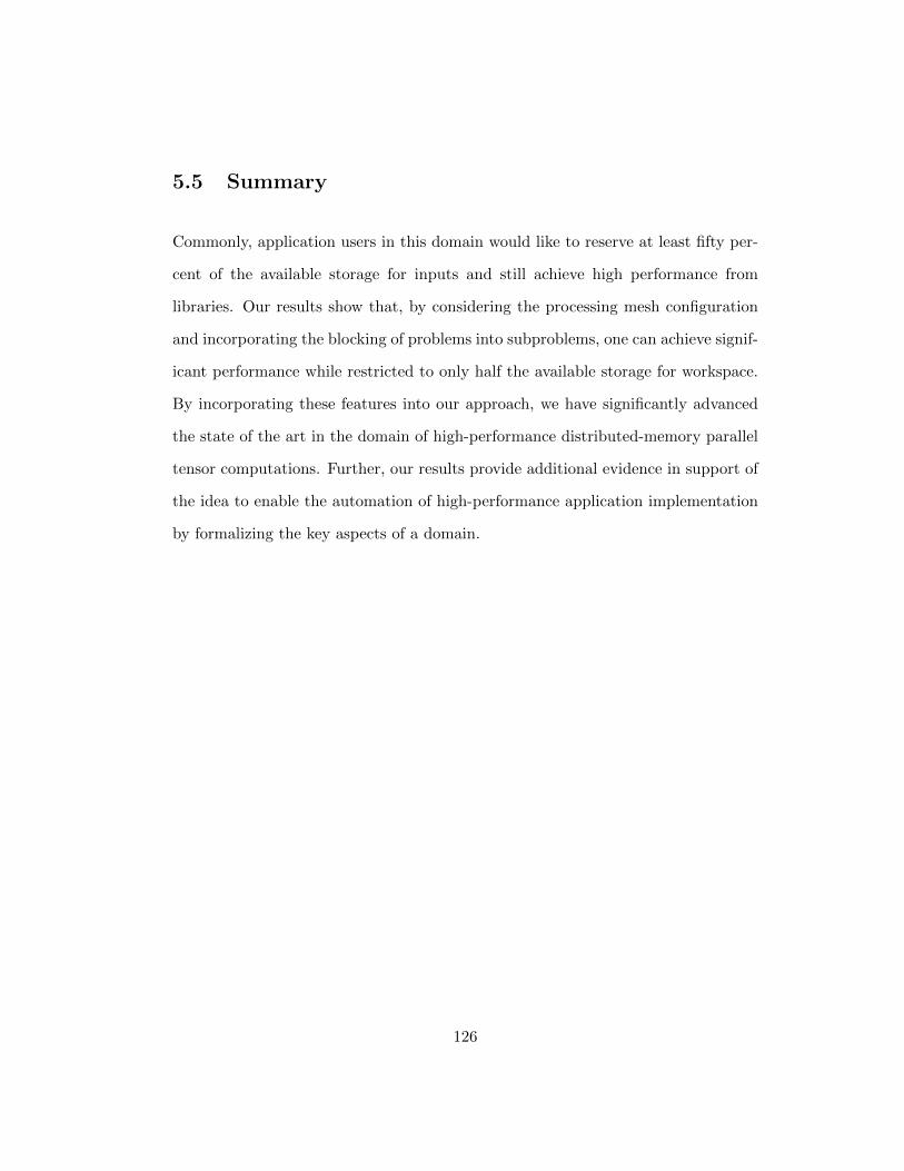
5.5 Summary

Commonly, application users in this domain would like to reserve at least fifty per-

cent of the available storage for inputs and still achieve high performance from

libraries. Our results show that, by considering the processing mesh configuration

and incorporating the blocking of problems into subproblems, one can achieve signif-

icant performance while restricted to only half the available storage for workspace.

By incorporating these features into our approach, we have significantly advanced

the state of the art in the domain of high-performance distributed-memory parallel

tensor computations. Further, our results provide additional evidence in support of

the idea to enable the automation of high-performance application implementation

by formalizing the key aspects of a domain.

126

Chapter 6

Related Work

In this chapter, we compare approaches and ideas in other projects related to those

in this thesis.

6.1 Tensor Contraction Engine (TCE)

The Tensor Contraction Engine project (circa 2005) [8, 35, 36, 37], a part of the

NWChem package for computational chemistry [14, 84], is perhaps the first project

of its kind with the goal of automating the task of creating high-performance

distributed-memory implementations for applications based on tensor contractions.

In fact, many important aspects of designing high-performance implementations in

this domain originated in TCE. As such, it can be considered the precursor to many

of the other projects discussed in this chapter.

The overarching goal of TCE is to create a distributed-memory implementation for a

problem specification that performs the fewest number of operations in the available

127

space. To do this, TCE searches a space of algorithms created by iteratively apply-

ing a series of transformations and analyses until it either finds a valid algorithm

or halts having found no viable algorithm. The applied transformations include

algebraic transformations that manipulate the number of required operations to im-

plement the problem specification. One side effect of manipulating the number of

required operations is that the storage requirements of the devised method can also

be affected (either increase or decrease). For this, transformations and analyses re-

lated to compiler techniques consider how to manipulate the storage requirements;

these include transformations related to loop fusion and those that consider the

addition/removal of temporary variables.

If an algorithm is selected for implementation, TCE synthesizes implementations

that rely on dynamic scheduling to maintain load-balance among processes [35,

46, 63]. This is done because the arithmetic complexity associated with different

tensor contractions in a typical application can vary greatly, making approaches that

utilize all processes for a single task wasteful. When assigned a task of work, each

process asynchronously retrieves the required data from other processes, performs

the computation, and updates the relevant portions of the output.

Other works relying on dynamic task scheduling for parallelizing tensor applications

include the Dynamically Load-balanced Tensor Contraction (DLTC) library [48].

In this work, a hierarchical view of the tasks is created, allowing for groups of

computations to be assigned to a single process. In doing so, a better balance of

load among processes can be achieved.

Most relevant to this dissertation is the approach TCE takes to perform and optimize

the distributed computations. Contrary to the approach developed here, tensors

are interpreted as matrices when distributed (they are “flattened”). Because the

128

distributed computation proceeds based on Cannon’s algorithm, redistributions are

implemented via permutation collectives. Optimizations to reduce communication

are then applied when it is determined that specific tensor operands need not be

redistributed for the computation to proceed. As such, only the redistributions

required to prepare each operand for subsequent computations are optimized; TCE

does not examine the redistributions required by the distributed tensor contraction

algorithm in conjunction with those required for subsequent contractions.

In this work, we develop a notation and language that describes how distributed

computations must proceed and how redistributions can efficiently be implemented

(even optimized). With this knowledge encoded, we can optimize a series of compu-

tations together. Most relevant to the comparison with TCE is that an automated

system, having encoded the ideas developed in this document, can perform commu-

nication optimizations similar to what TCE does as well as optimizations that TCE

cannot currently perform.

We mention here that transformations utilized by TCE, such as the algebraic trans-

formations, are not considered in this work. As such, one key difference between

these two works is that here we assume the given problem specification is optimized

already, whereas TCE can perform that optimization itself.

6.2 Advanced Concepts in Electronic Structure III

(ACES III)

The Advanced Concepts in Electronic Structure (circa 2011) [23] is a package that

provides parallel implementations for various methods from computational chem-

129

istry that are written in the Super Instruction Assembly Language (SIAL) and are

computed using the Super Instruction Processor (SIP) [71]. The SIP has both static

and runtime system components that are used in conjunction to implement tensor

contractions written in SIAL. We mention here that the level of abstraction exposed

by SIAL is vastly different from that exposed by the current work. In this work,

we consider entire distributed objects and derive algorithms for entire computations

(applying blocking when necessary); whereas, in ACES and SIAL, the user must

reason about each block of data.

Perhaps the most distinct aspect of ACES compared to this work is that ACES relies

on a master-slave paradigm for data redistribution. The master initially determines

how data should be distributed among processes and then handles all redistribution

requests. Because of this design decision, redistributions cannot effectively utilize

the underlying communication network as a single process is responsible for orches-

trating the required redistributions. The burden on the master process increases

as processes are added to the system, thereby decreasing the ability to effectively

utilize the communication network. It is for this reason that we do not compare

against ACES III.

6.3 Cyclops Tensor Framework (CTF)

The Cyclops Tensor Framework (circa 2014) [81] is a high-performance distributed-

memory library developed for both dense and sparse tensor contraction compu-

tations that supports forms of tensor symmetry. As the ideas developed in this

dissertation do not presently support sparse data structures or forms of symmetry,

we focus on the aspects of CTF that pertain to dense, non-symmetric tensors.

130

Given a problem specified as a series of tensor contractions, CTF computes a single

contraction at a time, handling data distribution, redistribution, and algorithm

choice internally. As with this work, CTF relies on elemental-cyclic distributions

of data. In contrast to this work that encodes several collective communications,

redistributions of data between contraction operations in CTF are implemented

via all-to-all collectives and redistributions performed within a distributed tensor

contraction only rely on those specified by the chosen algorithm (typically broadcast,

permutation, and reduction collectives).

The specific algorithm chosen by CTF for computing the current tensor contraction

is based on a cost model analysis of different combinations of generalized SUMMA

algorithms and 3D-like parallel algorithms for matrix-matrix multiplication. More

specifically, CTF considers a nested form of SUMMA algorithms (one algorithm for

each stationary variant) in conjunction with replication-based 3D-like algorithms

that replicate the smallest tensor operand in order to reduce the amount of commu-

nication overhead.

As CTF separates the communications between distributed tensor contractions from

communications as part of the tensor contraction algorithm, redistributions cannot

be optimized across a series of tensor contractions at once. This is another difference

between CTF and the work of this dissertation.

131

6.4 RRR and The Contraction Algorithm for

Symmetric Tensors (CAST)

The RRR framework1 (circa 2014) [70] is a high-performance distributed-memory

library designed for dense tensor contractions. Computations involving tensors with

forms of symmetry are supported through the Contraction Algorithm for Symmetric

Tensors (CAST) [69], which is built on the RRR framework. Here, we discuss ideas

underlying the RRR as they apply to CAST as well.

The underlying idea behind RRR is similar in spirit to those discussed in this doc-

ument. RRR relies on elemental-cyclic data distributions and for redistribution

relies on three communication primitives that are implemented via pipelined ver-

sions (when applicable) of reduction, broadcast, and all-to-all collectives; the three

primitives are: reduction, recursive broadcast, and rotation. Additionally, RRR

derives algorithms for individual tensor contraction operations that follow the pat-

tern of redistributing data, performing local computations, and finally performing

any final redistributions. RRR considers a space of algorithms created by applying

the derivation process to all possible distributions of operands and selects the best

according to a cost model.

The derivation process utilized by RRR is more like recursion, in comparison to the

derivation method developed in this document that is akin to constraint propaga-

tion [44]. As part of the underlying theory, RRR defines a set of valid tensor mode

distributions of paired tensor modes that can be involved in a distributed computa-

tion and defines the necessary redistributions that enable valid local computations.

1The RRR framework is named after the communication primitives utilized: reduction, recursivebroadcast, and rotation.

132

The combination of redistributions and local computations to be performed de-

pends on the relationship between the pair of tensor modes being considered. The

distributed contraction algorithm then becomes a recursive application of this pro-

cess to each set of paired tensor modes. As a result of this approach, RRR can

consider generalizations of SUMMA algorithms, 3D-like algorithms, and Cannon’s

algorithm for computation. Contrast this approach to that taken in this work where

we consider the entire tensor distribution of each object together and propagate in-

formation until we arrive at a valid algorithm.

As with CTF, RRR only considers how to optimize communications in individual

tensor contractions and between pairs of contractions; optimizing a series tensor

contractions at once is not supported yet.

6.5 Elemental

The Elemental project (circa 2012) [65] is a high-performance distributed-memory

library for dense linear algebra. Elemental relies on elemental-cyclic and block-cyclic

distributions of data and formalizes both data distributions and redistributions in

terms of collective communications.

As we have mentioned throughout this document, the ideas in this work are heavily

influenced by those underlying Elemental, except that the ideas for distribution and

redistribution are generalized to support arbitrary-order tensors on arbitrary-order

processing meshes. Additionally, the ideas underlying how algorithms for matrix-

matrix multiplication in Elemental have been made systematic.

We mention here that it is due to the rigor behind the ideas in Elemental that made

133

key insights in this dissertation possible.

6.6 Summary

In this chapter we summarized works related to the ideas developed in this disserta-

tion. As we have discussed in the relevant sections, a significant difference between

our work and these projects is that our work facilitates the optimization of a series of

tensor contractions at once, instead only optimizing tensor contractions individually.

This is facilitated by the fact that the process of algorithm derivation is described

in the same notation as that used for distribution and redistribution.

134

Chapter 7

Conclusion

In this chapter, we summarize our results and mention opportunities for future

research.

7.1 Contributions

In this dissertation, we presented a notation that formalizes three major aspects

of distributed-memory parallel algorithm design for tensor contractions of dense,

non-symmetric tensors: data distribution, redistribution, and algorithm derivation.

This facilitated the automatic generation of high-performance implementations for

a series of tensor contractions. The defined notation was implemented in an API

(ROTE). The knowledge from this dissertation was encoded into the prototype sys-

tem DxTer to create high-performance implementations for the spin-adapted CCSD

method from computational chemistry. A post-processing step was applied to block

the computations to reduce the required workspace.

135

We now, in more detail, present the major achievements and contributions of this

dissertation.

7.1.1 A Notation for Data Distributions of Tensors

Data distribution is required when computing on distributed-memory systems. As

discussed in Section 2.3, this dissertation focused on elemental-cyclic distributions

of elements as they have been shown to be useful in many areas of high-performance

computing. As done in Elemental for matrices, this work related the idea of a data

distribution to that of a set partition [73]. Using this underlying idea, a general

notation was developed to express arbitrary-order tensors distributed on arbitrary-

order processing meshes that concisely expresses the pertinent information.

7.1.2 A Notation for Data Redistributions of Tensors

Effective use of collective communications for data redistribution is at the heart of

bulk synchronous parallel algorithms like those encountered in this domain. This

work links a broad set of collective communications to the redistributions expressed

with the defined notation. In doing so, we provided a useful abstraction for experts

when considering how data moves among processes. Care was taken to only choose

collective communications that are balanced. As such, an expert can more easily

determine how to efficiently implement an arbitrary redistribution.

136

7.1.3 A Generalization of Transformations

for Improving Performance

When tasked with optimizing an application for performance, experts wish to utilize

every technique known to them to improve performance. In Chapter 4, we demon-

strated the utility and expressiveness of the defined notation by generalizing and

formalizing a series of transformations that, in certain situations, can significantly

improve the predicted cost of the application. This provides a general set of tech-

niques to use, enabling the expert to quickly transform implementations into what

is predicted to be more efficient implementations.

7.1.4 A Systematic Method for Algorithm Derivation

Recognizing that different algorithmic variants are more appropriate than others in

certain situations, we developed a systematic approach to deriving members of a

family of algorithms. With this, the number of considerations required by a (human

or mechanical) expert when designing algorithms with efficient implementations can

be significantly reduced.

7.1.5 An API for Distributed Tensor Library Development

The ideas presented in this document were implemented in the ROTE API for

distributed-memory parallel tensor computations. The ROTE API is designed to

be a one-to-one mapping from the ideas presented here, allowing a simple transition

from developed algorithms in the notation to corresponding implementation.

137

7.1.6 An Advancement in State-of-the-Art

Tensor Computations

The ideas presented in this document were tested by applying them to the spin-

adapted CCSD method from computational chemistry using the DxTer prototype

system for code generation. Results from these experiments show that the ideas

in this document can significantly improve upon the state of the art in terms of

both performance and memory usage (in some cases a fifty percent improvement

in performance in conjunction with a factor three improvement in memory). In

addition, this demonstrates that the ideas and ROTE API can be incorporated into

existing tools for automatic code generation.

7.1.7 A New Case Study for DxTer

The utility and flexibility of automated tools and software-engineering methodolo-

gies must be demonstrated for them to gain acceptance from a broader audience. As

leveraged in this work, both the utility and flexibility of DxTer were demonstrated

for the domain of distributed-memory applications based on tensor contractions,

thereby providing a new case study for DxTer. The ideas developed in this docu-

ment provide the required knowledge for DxTer to be applied.

7.2 Future Work

Here we discuss topics for future research related to this dissertation.

138

7.2.1 Symmetry

The most important feature lacking in this work is the consideration of symmet-

ric objects for distribution. Certain applications in computational chemistry that

require tensor contractions, such as CCSDT(Q) [47, 62], exploit this feature. We

will investigate how to incorporate symmetry into the notation and theory in future

research.

7.2.2 Sparsity

In addition to symmetry, some methods rely on sparsity in the tensors to reduce the

overall computational cost and storage requirements [31, 42, 52]. A key benefits of

only considering dense tensors is that each process can be assigned a predictable and

structured set of elements while maintaining balance (in computation and storage)

among processes. We plan to investigate what forms of sparsity can be incorporated

in the developed notation, thereby supporting a broader set of applications.

7.2.3 Additional Families of Algorithms

As argued in this dissertation, incorporating families of algorithms is crucial to

tailoring implementations. In this work, we focused on the stationary family of al-

gorithms; however, so-called 3D families of algorithms [2, 73, 79] for matrix-matrix

multiplication have benefits in certain settings and generalizations have been incor-

porated into other related projects. We will investigate how to incorporate that

family, and other potential families, of algorithms in the developed notation as part

of future research.

139

7.2.4 Additional Data Distributions

We chose to focus on formalizing elemental-cyclic distributions. Other projects

rely on different forms of Cartesian distributions [8, 23] and other applications as

well. For instance, some chemistry methods rely on distributions that are more like

blocked distributions than elemental-cyclic [9]. We plan to investigate how different

Cartesian distributions can be incorporated in the defined notation as well as the

potential benefits of doing so in future research.

7.2.5 Generalizations of the Derivation Process

In Chapter 3, we presented a procedure for algorithm derivation that expresses

the elementwise definition of a tensor contraction as a two-step approach: first,

specifying the local computations to be performed; second, specifying the global

accumulations needed. It is unclear if there are benefits to converting the original

elementwise definition to a different two-step, or a multi-step, approach. We will

investigate this in future research.

7.2.6 Additional Optimizing Transformations

We discussed how the notation can describe two optimizing transformations to im-

prove performance of redistributions in Chapter 4. We plan to investigate if other

transformations can be expressed. Additionally, we plan to investigate if there are

other communication patterns that should be described by the current notation.

Doing so would create additional knowledge that automated systems can utilize for

reasoning or provide knowledge that can reduce the space of choices to consider

when optimizing an application.

140

7.2.7 Additional Tensor Operations

The application focused on in this dissertation arises from computational chemistry

and the operation investigated was the tensor contraction. Tensor operations, such

as factorizations, have also been shown to arise in the area of data analysis [4, 5, 45].

As part of future research, we plan to investigate how to incorporate these operations

into the defined notation and formalism.

7.2.8 Heuristics for Reducing the Space of Implementations

There is opportunity to generalize the insights discussed in Chapter 4 so that

arbitrary redistributions (including reduction, duplication, and intentional load-

imbalance) can be efficiently implemented. Systematically determining an efficient

composition of redistribution rules to implement an arbitrary redistribution can sig-

nificantly limit the search space needed to be considered by the (human or mechan-

ical) expert. We will investigate the feasibility of this idea as well as the potential

impact on implementation generation.

7.2.9 Aiding Automated Tools

As demonstrated in Section 5.4.4, blocking computations into subproblems can

significantly reduce the amount of workspace required for computation. In Sec-

tion 3.2.2, we gave guidance for selecting the correct tensor modes to block along.

Presently, the process of blocking computations was performed as a post-processing

step after an efficient implementation was generated. Incorporating this knowledge

of blocking into automated systems provides additional expert knowledge with which

to make decisions.

141

Appendices

142

Appendix A

Proofs of Redistribution Rules

In this appendix, we prove that each of the redistribution rules given in Figure 2.14

and Figure 2.15 can be implemented via balanced forms of simultaneous invocations

of the associated collective communication communicating over the specified set

of processing mesh modes. We assume an offset parameter of σ = 0 as minor

modifications can be made to the proofs to enable arbitrary assignments of σ.

A.1 Proofs of Correctness Strategy

Recall that when we say that a redistribution is performed or communicated “over

modes D of G”, we mean that multiple instances of the associated collective are

invoked simultaneously with each instance involving all processes whose locations

in G only differ in the modes specified by D.

For example, performing a redistribution associated with the allgather collective

over modes D = (2, 0) of the order-4 processing mesh G means that simultaneous

143

allgather instances are invoked, each involving all processes whose locations in G

differ only in mode 0 and mode 2. As a result, a redistribution performed over modes

D of a N -order processing mesh of size P involves prod(P,R (N) \ D

)simultaneous

invocations, each involving p = prod(P, D

)processes.

We can capture the interaction of processes involved in the same collective invocation

with four sets of processes

1. the set of processes involved in the same communication1, “peers”, denoted

Q,

2. the set of processes that send portions of the required data to be communi-

cated, “sources”, denoted S,

3. the set of processes that receive portions of the required data that is commu-

nicated, “targets”, denoted T , and

4. the subset of S from which each target q ∈ T obtains all required data,

“contributors”, denoted S(q).

.

By definition, any set of contributors must be a subset of the senders as only senders

can send data. Similarly, the set of senders and targets must be subsets of the peers.

For instance, in the case of the all-to-all collective, every process involved is a sender,

target, and the set of contributors for a given target is the entire set of senders. In

contrast, in the case of the permutation collective, every process is both a sender

and target, but each target must be assigned a single unique contributor. Observe

that Table A.1 summarizes the relationship between Q, S, T , and S(q) for each

1Group in MPI.

144

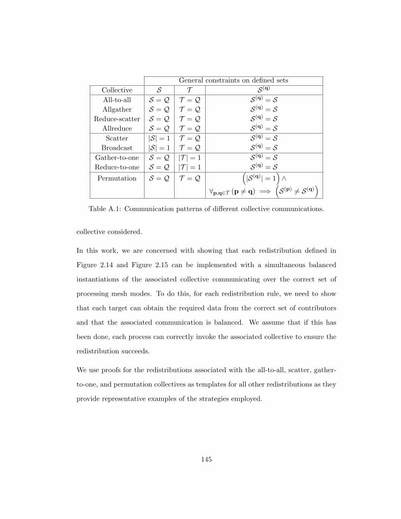
General constraints on defined sets

Collective S T S(q)

All-to-all S = Q T = Q S(q) = SAllgather S = Q T = Q S(q) = S

Reduce-scatter S = Q T = Q S(q) = SAllreduce S = Q T = Q S(q) = SScatter |S| = 1 T = Q S(q) = S

Broadcast |S| = 1 T = Q S(q) = SGather-to-one S = Q |T | = 1 S(q) = SReduce-to-one S = Q |T | = 1 S(q) = SPermutation S = Q T = Q

(|S(q)| = 1

)∧

∀p,q∈T (p 6= q) =⇒(S(p) 6= S(q)

)Table A.1: Communication patterns of different collective communications.

collective considered.

In this work, we are concerned with showing that each redistribution defined in

Figure 2.14 and Figure 2.15 can be implemented with a simultaneous balanced

instantiations of the associated collective communicating over the correct set of

processing mesh modes. To do this, for each redistribution rule, we need to show

that each target can obtain the required data from the correct set of contributors

and that the associated communication is balanced. We assume that if this has

been done, each process can correctly invoke the associated collective to ensure the

redistribution succeeds.

We use proofs for the redistributions associated with the all-to-all, scatter, gather-

to-one, and permutation collectives as templates for all other redistributions as they

provide representative examples of the strategies employed.

145

A.2 Lemmas

Consider a multiindex i, a size I, and the ordered sets A, B, and C such that

C = A t B. To help us more easily reason about where data resides under different

distributions, we must understand the relationship between the result prod (I, C) and

both the results prod (I,A) and prod (I,B) as well as the analogous relationship for

the multi2linear function involving i. Understanding these relationships is crucial to

the proofs of correctness for our defined redistributions. We define this relationship

for the prod function in Lemma 1.

Lemma 1. Given an order-M size array I, and an ordered set D t D, then

prod(I,D t D

)= prod (I,D) · prod

(I, D

).

Proof: IfM = 0, the claim trivially holds. Otherwise, let u(0) = I (D), u(1) = I(D)

,

and u = u(0) t u(1) = I(D t D

). By the definition of prod,

prod(I,D t D

)= prod

(I(D t D

))= prod (u)

=∏

`∈R(M)

u`

=∏

`∈R(|u(0)|)

u(0)` ·

∏`∈R(|u(1)|)

u(1)`

= prod(u(0)

)· prod

(u(1)

)= prod (I (D)) · prod

(I(D))

= prod (I,D) · prod(I, D

).

endofproof

146

We define the analogous relationship for the multi2linear function in Lemma 2.

Lemma 2. Given an order-M multiindex i, corresponding size array I, and an

ordered set D t D, then

multi2linear(i, I,D t D

)= multi2linear (i, I,D) +

multi2linear(i, I, D

)prod (I,D) .

Proof: IfM = 0, the claim trivially holds. Otherwise, let u(0) = i (D), u(1) = i(D)

,

and u = u(0) t u(1) = i(D t D

). Similarly define v(0), v(1), and v so that

v = I(D t D

). By definition of multi2linear and Lemma 1,

multi2linear(i, I,D t D

)= multi2linear

(i(D t D

), I(D t D

))= multi2linear (u,v)

=∑

`∈R(|u|)

u` · prod (v,R (`))

=∑

`∈R(|u(0)|)

u(0)` · prod

(v(0),R (`)

)+

∑`∈R(|u(1)|)

u(1)` · prod

(v(1),R (`)

)· prod

(v(0)

)= multi2linear

(u(0),v(0)

)+ multi2linear

(u(1),v(1)

)prod

(v(0)

)= multi2linear (i (D) , I (D))

+multi2linear(i(D), I(D))

prod (I (D))

= multi2linear (i, I,D)

+multi2linear(i, I, D

)prod (I,D) .

endofproof

147

A.3 Proofs of Correctness

One now establish the correspondance between each collective communication in

Figure 2.6 and its associated redistribution in Figure 2.14 and Figure 2.15.

A.3.1 All-to-all

Theorem 1. Consider an order-M tensor A of size I distributed on an order-N

processing grid G of size P. The redistribution

A[D(0), . . . ,D(v−1),D(v) t D(0), . . . ,D(M−1) t D(M−1−v); E , w

]↓

A[D(0) t D(0)

, . . . ,D(v−1) t D(v−1),D(v), . . . ,D(M−1); E , w

]where (v − 1) ∈ R (M) and π represents a permutation of entries, can

be performed via simultaneous all-to-all collectives communicating over modes⋃m∈R(M)

D(m) =⋃

m∈R(M)

D(m)in G.

Proof: We prove this for the simple case entries have not been permuted and

that E = ∅ and w = 0. Identical arguments can be made for other consistent

permutations, and assignment of E and w.

Let

D =(D(0), . . . ,D(v−1),D(v) t D(0), . . . ,D(M−1) t D(M−1−v)

),

D =(D(0) t D(0)

, . . . ,D(v−1) t D(v−1),D(v), . . . ,D(M−1)

),

148

D =⋃

m∈R(M−v)

D(m),

and

D =⋃

m∈R(M)

D(m).

Consider how an arbitrary all-to-all collective would proceed. We know how to

define the sets Q, S, and T .

Our first goal is to show that the required set of elements for each target q ∈ T

can be obtained from the associated set of contributors S(q) = Q. Our strategy is

to consider an arbitrary element required by q under D and construct a process p

such that p ∈ S and is assigned the same element under D.

Consider the target q ∈ T and the element at location i assigned to q under D.

Assign the entries of p in the modes specified by R (N) \ D to be the same as q.

This ensures that if q is assigned elements under D, then p is as well

Now, consider the mode m ∈ R (M) such that m < v. Notice that in this case

I(p)m

(D(m)

)⊇ I(q)m

(D(m) t D(m)

)

meaning that p is assigned the index im of mode m under D.

This argument can be applied for all other modes m < v. We ensure the same

location in p is not assigned more than once as, by definition, no two tensor mode

distributions can share the same entries meaning we only ever assign each entry of

p once.

149

Now consider the case where m ≥ v. Based on D, im is defined as

im = multi2linear(q,P,D(m)

)+ j(0)prod

(P,D(m)

)

for some non-negative integer j(0).

Recall that each mode-m index assigned to p under D can be defined as

multi2linear(p,P,D(m) t D(m−v)

)+ j(1)prod

(P,D(m) t D(m−v)

)

for some non-negative integer j(1).

By Lemma 2

multi2linear(p,P,D(m) t D(m−v)

)=

multi2linear(p,P,D(m)

)+ multi2linear

(p,P, D(m−v)

)prod

(P,D(m)

),

so each mode-m index assigned to p under D can also be defined as

multi2linear(p,P,D(m)

)+ multi2linear

(p,P, D(m−v)

)prod

(P,D(m)

)+ j(1)prod

(P,D(m) t D(m−v)

)

By Lemma 1 and Lemma 2, each mode-m index assigned to p under D can also be

defined as

multi2linear(p,P,D(m)

)+(

multi2linear(p,P, D(m−v)

)+ j(1)prod

(P, D(m−v)

))prod

(P,D(m)

)

150

Assign the entries of p in the modes specified by D(m−v) such that

multi2linear(p,P, D(m−v)

)≡ j(0)

(mod prod

(P, D(m−v)

)).

Notice that im ∈ I(p)m

(D(m) t D(m−v)

)as, based on our construction of p, we can

always choose a j(1) such that

j(0) = multi2linear(p,P, D(m−v)

)+ j(1)prod

(P, D(m−v)

)

and all other relevant entries of p are defined similarly to q. Therefore, p is assigned

the mode-m index im under D.

Applying this argument to all modes m ∈ R (M) defines the remaining entries for

p as D =⋃

m∈R(M−1−v)

D(m). Therefore, we have constructed a process p that is

assigned the element at location i under D. As p ∈ S, by Table A.1, we know that

p ∈ S(q).

endofproof

151

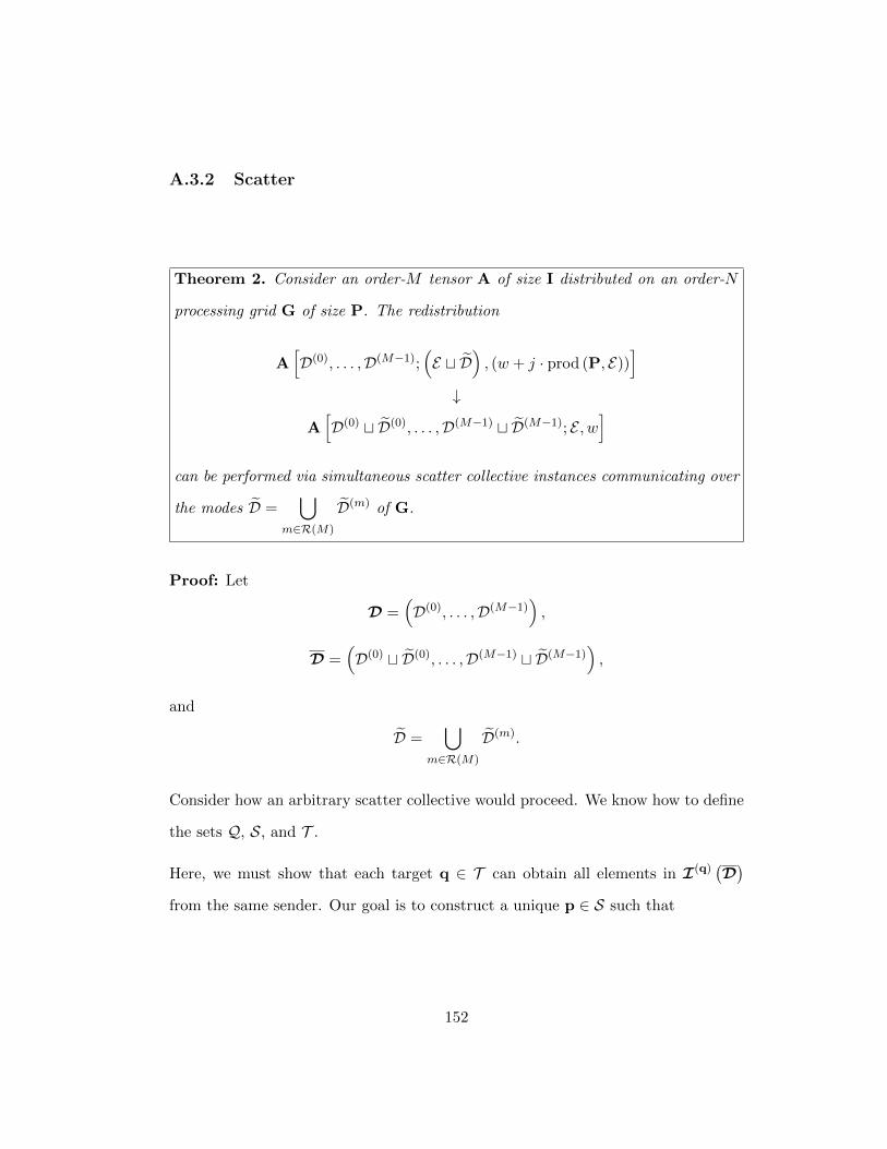
A.3.2 Scatter

Theorem 2. Consider an order-M tensor A of size I distributed on an order-N

processing grid G of size P. The redistribution

A[D(0), . . . ,D(M−1);

(E t D

), (w + j · prod (P, E))

]↓

A[D(0) t D(0), . . . ,D(M−1) t D(M−1); E , w

]can be performed via simultaneous scatter collective instances communicating over

the modes D =⋃

m∈R(M)

D(m) of G.

Proof: Let

D =(D(0), . . . ,D(M−1)

),

D =(D(0) t D(0), . . . ,D(M−1) t D(M−1)

),

and

D =⋃

m∈R(M)

D(m).

Consider how an arbitrary scatter collective would proceed. We know how to define

the sets Q, S, and T .

Here, we must show that each target q ∈ T can obtain all elements in I(q)(D)

from the same sender. Our goal is to construct a unique p ∈ S such that

152

I(q)(D; E , w

)⊆ I(p)

(D;(E t D

), w + j · prod (P, E)

).

for each q ∈ T .

By assigning the entries of p in the modes specified by R (N) \ D to the same as

those in q, we ensure that p ∈ Q.

By assigning the entries of p in the modes specified by D such that

j = multi2linear(p,P, D

)

then we know that p is assigned data under D if q is under D.

Notice that

I(q)(D; E , w

)⊆ I(p)

(D;(E t D

), w + j · prod (P, E)

)

meaning that under D, p is assigned all elements required by q under D. Therefore,

p ∈ S(q). Finally, notice that this is the case for any q ∈ T . Thus, p ∈ S and

|S| = 1. endofproof

153

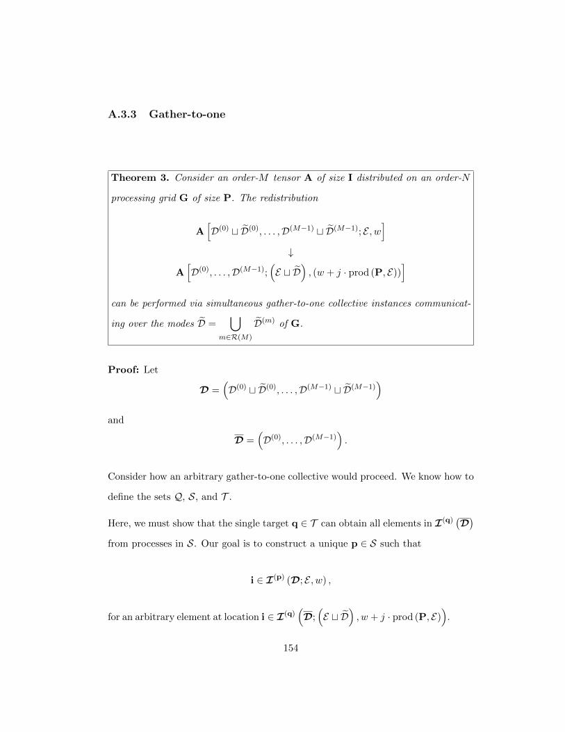
A.3.3 Gather-to-one

Theorem 3. Consider an order-M tensor A of size I distributed on an order-N

processing grid G of size P. The redistribution

A[D(0) t D(0), . . . ,D(M−1) t D(M−1); E , w

]↓

A[D(0), . . . ,D(M−1);

(E t D

), (w + j · prod (P, E))

]can be performed via simultaneous gather-to-one collective instances communicat-

ing over the modes D =⋃

m∈R(M)

D(m) of G.

Proof: Let

D =(D(0) t D(0), . . . ,D(M−1) t D(M−1)

)and

D =(D(0), . . . ,D(M−1)

).

Consider how an arbitrary gather-to-one collective would proceed. We know how to

define the sets Q, S, and T .

Here, we must show that the single target q ∈ T can obtain all elements in I(q)(D)

from processes in S. Our goal is to construct a unique p ∈ S such that

i ∈ I(p) (D; E , w) ,

for an arbitrary element at location i ∈ I(q)(D;(E t D

), w + j · prod (P, E)

).

154

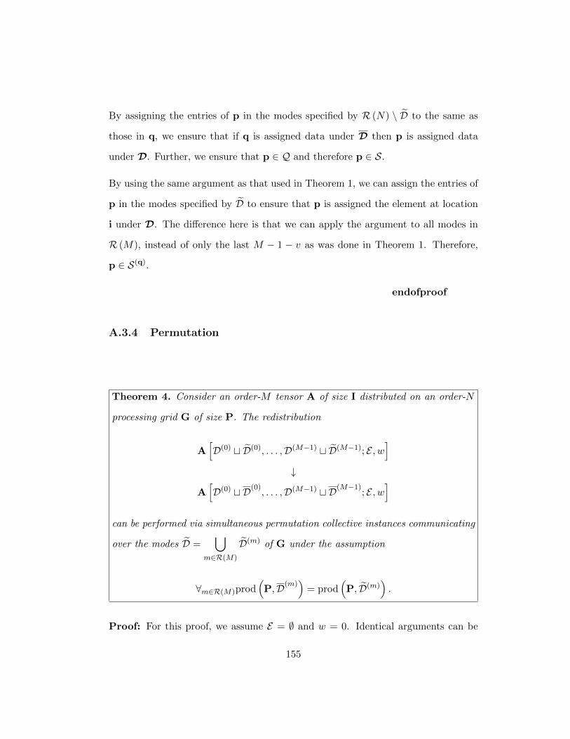
By assigning the entries of p in the modes specified by R (N) \ D to the same as

those in q, we ensure that if q is assigned data under D then p is assigned data

under D. Further, we ensure that p ∈ Q and therefore p ∈ S.

By using the same argument as that used in Theorem 1, we can assign the entries of

p in the modes specified by D to ensure that p is assigned the element at location

i under D. The difference here is that we can apply the argument to all modes in

R (M), instead of only the last M − 1 − v as was done in Theorem 1. Therefore,

p ∈ S(q).

endofproof

A.3.4 Permutation

Theorem 4. Consider an order-M tensor A of size I distributed on an order-N

processing grid G of size P. The redistribution

A[D(0) t D(0), . . . ,D(M−1) t D(M−1); E , w

]↓

A[D(0) t D(0)

, . . . ,D(M−1) t D(M−1); E , w

]can be performed via simultaneous permutation collective instances communicating

over the modes D =⋃

m∈R(M)

D(m) of G under the assumption

∀m∈R(M)prod(P,D(m)

)= prod

(P, D(m)

).

Proof: For this proof, we assume E = ∅ and w = 0. Identical arguments can be

155

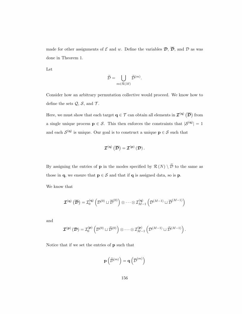
made for other assignments of E and w. Define the variables D, D, and D as was

done in Theorem 1.

Let

D =⋃

m∈R(M)

D(m).

Consider how an arbitrary permutation collective would proceed. We know how to

define the sets Q, S, and T .

Here, we must show that each target q ∈ T can obtain all elements in I(q)(D)

from

a single unique process p ∈ S. This then enforces the constraints that |S(q)| = 1

and each S(q) is unique. Our goal is to construct a unique p ∈ S such that

I(q)(D)

= I(p) (D) .

By assigning the entries of p in the modes specified by R (N) \ D to the same as

those in q, we ensure that p ∈ S and that if q is assigned data, so is p.

We know that

I(q)(D)

= I(q)0

(D(0) t D(0)

)⊗ · · · ⊗ I(q)M−1

(D(M−1) t D(M−1)

)

and

I(p) (D) = I(p)0

(D(0) t D(0)

)⊗ · · · ⊗ I(p)M−1

(D(M−1) t D(M−1)

).

Notice that if we set the entries of p such that

p(D(m)

)= q

(D(m)

)

156

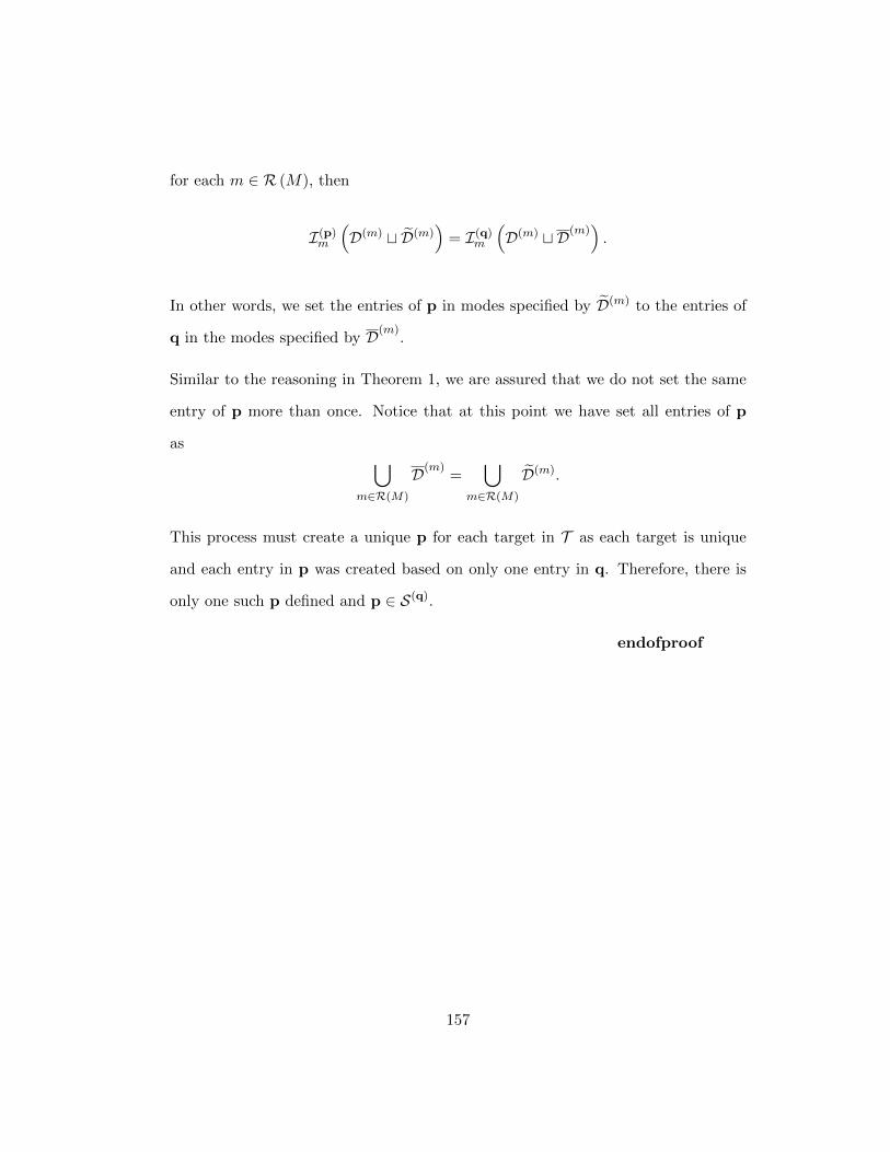
for each m ∈ R (M), then

I(p)m

(D(m) t D(m)

)= I(q)m

(D(m) t D(m)

).

In other words, we set the entries of p in modes specified by D(m) to the entries of

q in the modes specified by D(m).

Similar to the reasoning in Theorem 1, we are assured that we do not set the same

entry of p more than once. Notice that at this point we have set all entries of p

as ⋃m∈R(M)

D(m)=

⋃m∈R(M)

D(m).

This process must create a unique p for each target in T as each target is unique

and each entry in p was created based on only one entry in q. Therefore, there is

only one such p defined and p ∈ S(q).

endofproof

157

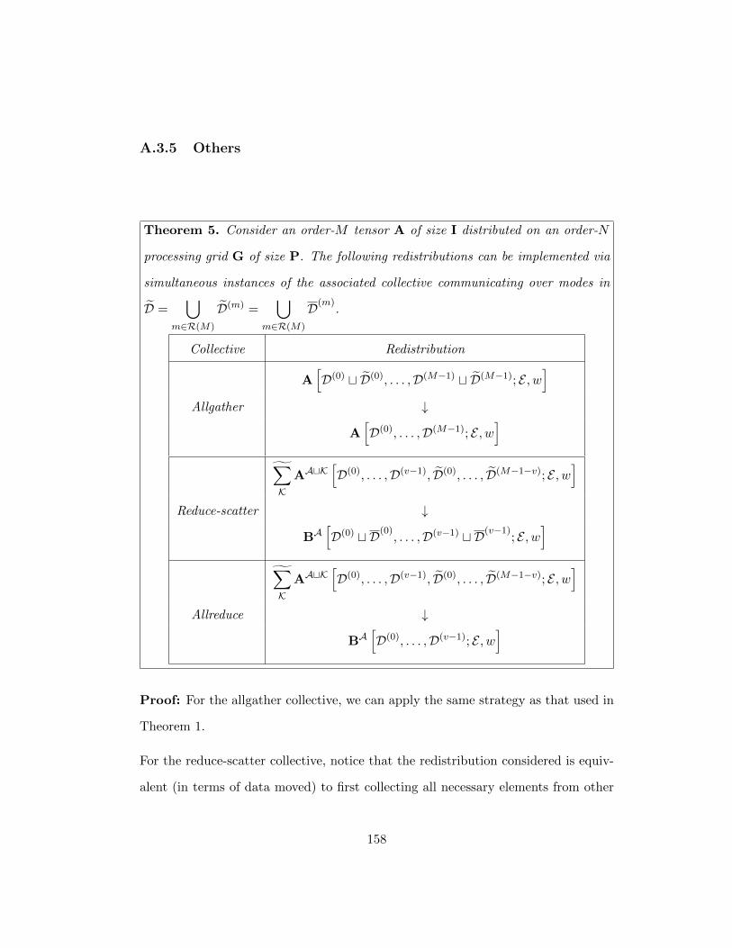
A.3.5 Others

Theorem 5. Consider an order-M tensor A of size I distributed on an order-N

processing grid G of size P. The following redistributions can be implemented via

simultaneous instances of the associated collective communicating over modes in

D =⋃

m∈R(M)

D(m) =⋃

m∈R(M)

D(m).

Collective Redistribution

A[D(0) t D(0), . . . ,D(M−1) t D(M−1); E , w

]Allgather ↓

A[D(0), . . . ,D(M−1); E , w

]∑K

AAtK[D(0), . . . ,D(v−1), D(0), . . . , D(M−1−v); E , w

]Reduce-scatter ↓

BA[D(0) t D(0)

, . . . ,D(v−1) t D(v−1); E , w

]∑K

AAtK[D(0), . . . ,D(v−1), D(0), . . . , D(M−1−v); E , w

]Allreduce ↓

BA[D(0), . . . ,D(v−1); E , w

]

Proof: For the allgather collective, we can apply the same strategy as that used in

Theorem 1.

For the reduce-scatter collective, notice that the redistribution considered is equiv-

alent (in terms of data moved) to first collecting all necessary elements from other

158

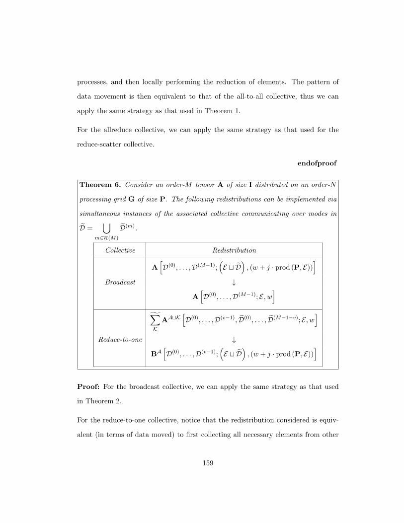
processes, and then locally performing the reduction of elements. The pattern of

data movement is then equivalent to that of the all-to-all collective, thus we can

apply the same strategy as that used in Theorem 1.

For the allreduce collective, we can apply the same strategy as that used for the

reduce-scatter collective.

endofproof

Theorem 6. Consider an order-M tensor A of size I distributed on an order-N

processing grid G of size P. The following redistributions can be implemented via

simultaneous instances of the associated collective communicating over modes in

D =⋃

m∈R(M)

D(m).

Collective Redistribution

A[D(0), . . . ,D(M−1);

(E t D

), (w + j · prod (P, E))

]Broadcast ↓

A[D(0), . . . ,D(M−1); E , w

]∑K

AAtK[D(0), . . . ,D(v−1), D(0), . . . , D(M−1−v); E , w

]Reduce-to-one ↓

BA[D(0), . . . ,D(v−1);

(E t D

), (w + j · prod (P, E))

]

Proof: For the broadcast collective, we can apply the same strategy as that used

in Theorem 2.

For the reduce-to-one collective, notice that the redistribution considered is equiv-

alent (in terms of data moved) to first collecting all necessary elements from other

159

processes, and then locally performing the reduction of elements. The pattern of

data movement is then equivalent to that of the gather-to-one collective, thus we

can apply the same strategy as that used in Theorem 3.

endofproof

A.4 Proofs of Balance

Here we prove that each of the rules defined in Figure 2.14 and Figure 2.15 corre-

spond to balanced communications. We focus only on the all-to-all redistribution

as all others rely on very similar arguments.

For these proofs, we must be assured that the distributions defined in the notation

balance the data among processes; that is, each process is assigned approximately

the same amount of data and all data entries are assigned to some process. An

argument based on the fact that the function multi2linear is bijective can be made

to show this.

A.4.1 All-to-all

160

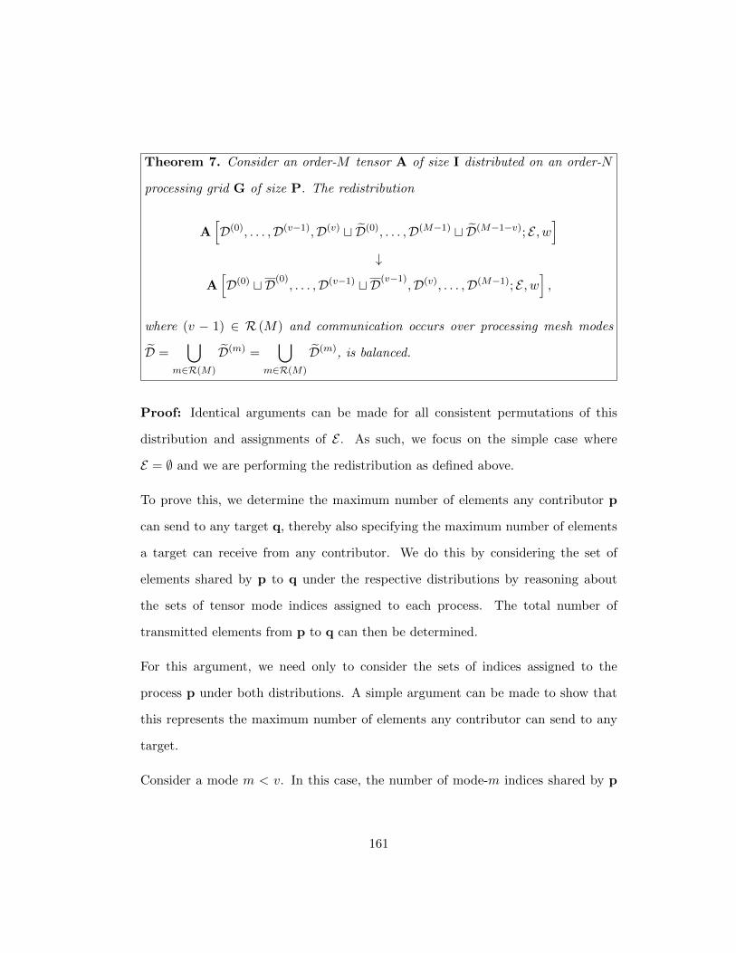
Theorem 7. Consider an order-M tensor A of size I distributed on an order-N

processing grid G of size P. The redistribution

A[D(0), . . . ,D(v−1),D(v) t D(0), . . . ,D(M−1) t D(M−1−v); E , w

]↓

A[D(0) t D(0)

, . . . ,D(v−1) t D(v−1),D(v), . . . ,D(M−1); E , w

],

where (v − 1) ∈ R (M) and communication occurs over processing mesh modes

D =⋃

m∈R(M)

D(m) =⋃

m∈R(M)

D(m), is balanced.

Proof: Identical arguments can be made for all consistent permutations of this

distribution and assignments of E . As such, we focus on the simple case where

E = ∅ and we are performing the redistribution as defined above.

To prove this, we determine the maximum number of elements any contributor p

can send to any target q, thereby also specifying the maximum number of elements

a target can receive from any contributor. We do this by considering the set of

elements shared by p to q under the respective distributions by reasoning about

the sets of tensor mode indices assigned to each process. The total number of

transmitted elements from p to q can then be determined.

For this argument, we need only to consider the sets of indices assigned to the

process p under both distributions. A simple argument can be made to show that

this represents the maximum number of elements any contributor can send to any

target.

Consider a mode m < v. In this case, the number of mode-m indices shared by p

161

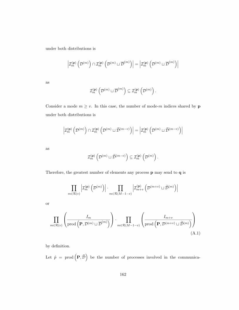
under both distributions is

∣∣∣I(p)m

(D(m)

)∩ I(p)m

(D(m) t D(m)

)∣∣∣ =∣∣∣I(p)m

(D(m) t D(m)

)∣∣∣as

I(p)m

(D(m) t D(m)

)⊆ I(p)m

(D(m)

).

Consider a mode m ≥ v. In this case, the number of mode-m indices shared by p

under both distributions is

∣∣∣I(p)m

(D(m)

)∩ I(p)m

(D(m) t D(m−v)

)∣∣∣ =∣∣∣I(p)m

(D(m) t D(m−v)

)∣∣∣as

I(p)m

(D(m) t D(m−v)

)⊆ I(p)m

(D(m)

).

Therefore, the greatest number of elements any process p may send to q is

∏m∈R(v)

∣∣∣I(p)m

(D(m)

)∣∣∣ · ∏m∈R(M−1−v)

∣∣∣I(p)m+v

(D(m+v) t D(m)

)∣∣∣or

∏m∈R(v)

Im

prod(P,D(m) t D(m)

) · ∏

m∈R(M−1−v)

Im+v

prod(P,D(m+v) t D(m)

)

(A.1)

by definition.

Let p = prod(P, D

)be the number of processes involved in the communica-

162

tion.

The maximum number of elements assigned to any one process under D is

n =∏

m∈R(v)

Im

prod(P,D(m) t D(m)

) · ∏

m∈R(M−1−v)

(Im+v

prod(P,D(m+v)

)) . (A.2)

Notice that the ratio between (A.1) and (A.2) is a factor

p =∏

m∈R(M−1−v)

prod(P, D(m)

).

Using the interpretation of Figure 2.7, if all p processes can contribute approxi-

mately the same amount of data to all other processes, then the associated sub-

vectors assigned to each process are approximately the same size. Therefore, the

communication is balanced. endofproof

163

Bibliography

[1] OpenBLAS. http://xianyi.github.com/OpenBLAS/, 2012.

[2] R. C. Agarwal, S. M. Balle, F. G. Gustavson, M. Joshi, and P. Palkar. A

three-dimensional approach to parallel matrix multiplication. IBM Journal of

Research and Development, 39(5):575–582, 1995.

[3] R. C. Agarwal, F. Gustavson, and M. Zubair. A high-performance matrix multi-

plication algorithm on a distributed memory parallel computer using overlapped

communication. IBM Journal of Research and Development, 38(6):673–681,

1994.

[4] C. M. Andersen and R. Bro. Practical aspects of PARAFAC modeling of flu-

orescence excitation-emission data. Journal of Chemometrics, 17(4):200–215,

2003.

[5] B. W. Bader, M. W. Berry, and M. Browne. Discussion tracking in Enron email

using PARAFAC. In Michael W. Berry and Malu Castellanos, editors, Survey

of Text Mining II, pages 147–163. Springer London, 2008.

[6] G. Ballard, J. Demmel, L. Grigori, M. Jacquelin, H. D. Nguyen, and

E. Solomonik. Reconstructing Householder vectors from Tall-Skinny QR. In

164

Proceedings of the IEEE 28th International Parallel and Distributed Processing

Symposium, IPDPS ’14, pages 1159–1170. IEEE Computer Society, 2014.

[7] R. J. Bartlett. Many-body perturbation theory and coupled cluster theory

for electron correlation in molecules. Annual Review of Physical Chemistry,

32(1):359–401, 1981.

[8] G. Baumgartner, A. Auer, D. E. Bernholdt, A. Bibireata, V. Choppella, D. Co-

ciorva, X. Gao, R. J. Harrison, S. Hirata, S. Krishnamoorthy, S. Krishnan,

C. Lam, Q. Lu, M. Nooijen, R. M. Pitzer, J. Ramanujam, P. Sadayappan, and

A. Sibiryakov. Synthesis of high-performance parallel programs for a class of

ab initio quantum chemistry models. Proceedings of the IEEE, 93(2):276–292,

2005.

[9] N. H. F. Beebe and J. Linderberg. Simplifications in the generation and trans-

formation of two-electron integrals in molecular calculations. International

Journal of Quantum Chemistry, 12(4):683–705, 1977.

[10] G. Belter, E. R. Jessup, I. Karlin, and J. G. Siek. Automating the generation

of composed linear algebra kernels. In Proceedings of the Conference on High

Performance Computing Networking, Storage and Analysis, SC ’09, pages 59:1–

59:12. ACM, 2009.

[11] R. H. Bisseling. Parallel iterative solution of sparse linear systems on a trans-

puter network. In A. E. Fincham and B. Ford, editors, Parallel Computation,

volume 46 of The Institute of Mathematics and its Applications Conference,

pages 253–271. Oxford University Press, Oxford, UK, 1993.

[12] R. H. Bisseling and W. F. McColl. Scientific computing on bulk synchronous

parallel architectures. In B. Pehrson and I. Simon, editors, Proceedings of the

165

28th Annual Hawaii International Conference on System Sciences, volume 51 of

IFIP Transactions A, pages 509–514. Elsevier Science Publishers, Amsterdam,

1994.

[13] J. Bruck, C.-T. Ho, S. Kipnis, E. Upfal, and D. Weathersby. Efficient algorithms

for all-to-all communications in multi-port systems. In IEEE Transactions on

Parallel and Distributed Systems, pages 298–309, 1997.

[14] E. J. Bylaska, W. A. de Jong, N. Govind, K. Kowalski, T. P. Straatsma, and

M. Valiev. NWChem, a computational chemistry package for parallel comput-

ers, version 6.3.

[15] L. E. Cannon. A Cellular Computer to Implement the Kalman Filter Algorithm.

PhD thesis, Montana State University, Bozeman, MT, USA, 1969.

[16] E. Chan, M. Heimlich, A. Purkayastha, and R. van de Geijn. Collective com-

munication: theory, practice, and experience. Concurrency and Computation:

Practice and Experience, 19(13):1749–1783, 2007.

[17] J. Choi. A fast scalable universal matrix multiplication algorithm on

distributed-memory concurrent computers. In Proceedings of the 11th Inter-

national Symposium on Parallel Processing, IPPS ’97, pages 310–314. IEEE

Computer Society, 1997.

[18] J. Choi, J. J. Dongarra, R. Pozo, and D. W. Walker. ScaLAPACK: A scal-

able linear algebra library for distributed memory concurrent computers. In

Proceedings of the Fourth Symposium on the Frontiers of Massively Parallel

Computation, pages 120–127. IEEE Computer Society Press, 1992.

[19] J. Choi, D. W. Walker, and J. Dongarra. PUMMA: Parallel Universal Ma-

166

trix Multiplication Algorithms on distributed memory concurrent computers.

Concurrency: Practice and Experience, 6:543–570, 1994.

[20] J. Cızek. On the correlation problem in atomic and molecular systems. calcula-

tion of wavefunction components in Ursell-type expansion using quantum-field

theoretical methods. The Journal of Chemical Physics, 45(11):4256–4266, 1966.

[21] T. D. Crawford and H. F. Schaefer. An Introduction to Coupled Cluster Theory

for Computational Chemists. John Wiley & Sons, Inc., 2007.

[22] Cray. CrayXC30. http://www.cray.com/Assets/PDF/products/xc/

CrayXC30PDCProductBrief.pdf, 2013.

[23] E. Deumens, V. F. Lotrich, A. Perera, M. J. Ponton, B. A. Sanders, and R. J.

Bartlett. Software design of ACES III with the super instruction architecture.

Wiley Interdisciplinary Reviews: Computational Molecular Science, 1(6):895–

901, 2011.

[24] E. W. Dijkstra. A Discipline of Programming. Prentice Hall PTR, Upper

Saddle River, NJ, USA, 1st edition, 1997.

[25] C. Edwards, P. Geng, A. Patra, and R. van de Geijn. Parallel matrix dis-

tributions: Have we been doing it all wrong? Technical Report TR-95-40,

Department of Computer Sciences, The University of Texas at Austin, 1995.

[26] A. Einstein. Die Grundlage der allgemeinen Relativitatstheorie. Annalen der

Physik, 354:769–822, 1916.

[27] G. Fox, M. Johnson, G. Lyzenga, S. Otto, J. Salmon, and D. Walker. Solving

Problems on Concurrent Processors, volume I. Prentice Hall, 1988.

167

[28] K. Goto and R. van de Geijn. High-performance implementation of the level-3

BLAS. ACM Transactions on Mathematical Software, 35(1):4:1–4:14, 2008.

[29] K. Goto and R. A. van de Geijn. Anatomy of high-performance matrix mul-

tiplication. ACM Transactions on Mathematical Software, 34(3):12:1–12:25,

2008.

[30] J. Gunnels, C. Lin, G. Morrow, and R. van de Geijn. A flexible class of par-

allel matrix multiplication algorithms. In Proceedings of First Merged Inter-

national Parallel Processing Symposium and Symposium on Parallel and Dis-

tributed Processing (1998 IPPS/SPDP ’98), pages 110–116, 1998.

[31] T. Hazan, S. Polak, and A. Shashua. Sparse image coding using a 3D non-

negative tensor factorization. In Proceedings of the 10th IEEE International

Conference on Computer Vision, volume 1, pages 50–57, 2005.

[32] T. Helgaker, P. Jørgensen, and J. Olsen. Molecular Electronic Structure Theory.

John Wiley & Sons, Ltd., Chichester, 2000.

[33] B. Hendrickson, E. Jessup, and C. Smith. Toward an efficient parallel eigen-

solver for dense symmetric matrices. SIAM Journal on Scientific Computing,

20(3):1132–1154, 1998.

[34] B. Hendrickson, R. Leland, and S. Plimpton. An efficient parallel algorithm for

matrix-vector multiplication. International Journal of High Speed Computing,

7:73–88, 1995.

[35] S. Hirata. Tensor contraction engine: abstraction and automated parallel im-

plementation of configuration-interaction, coupled-cluster, and many-body per-

168

turbation theories. The Journal of Physical Chemistry A, 107(46):9887–9897,

2003.

[36] S. Hirata. Higher-order equation-of-motion coupled-cluster methods. The Jour-

nal of Chemical Physics, 121(1):51–59, 2004.

[37] S. Hirata. Symbolic algebra in quantum chemistry. Theoretical Chemistry

Accounts, 116(1-3):2–17, 2006.

[38] S. Huss-Lederman, E. Jacobson, and A. Tsao. Comparison of scalable parallel

matrix multiplication libraries. In Proceedings of the Scalable Parallel Libraries

Conference, pages 142–149, 1993.

[39] S. Huss-Lederman, E. Jacobson, A. Tsao, and G. Zhang. Matrix multiplica-

tion on the Intel Touchstone DELTA. Concurrency: Practice and Experience,

6(7):571–594, 1994.

[40] Intel. Reference manual for Intel Math Kernel Library; update 2, 2015.

[41] D. Irony, S. Toledo, and A. Tiskin. Communication lower bounds for

distributed-memory matrix multiplication. Journal of Parallel and Distributed

Computing, 64(9):1017–1026, 2004.

[42] H. A. L. Kiers, J. M. F. ten Berge, and R. Rocci. Uniqueness of three-mode

factor models with sparse cores: The 3x3x3 case. Psychometrika, 62(3):349–

374, 1997.

[43] J. Kim, W.J. Dally, S. Scott, and D. Abts. Technology-driven, highly-scalable

dragonfly topology. In Proceedings of the 35th International Symposium on

Computer Architecture, pages 77–88. IEEE Computer Society, 2008.

169

[44] D. E. Knuth. Semantics of context-free languages. Mathematical Systems The-

ory, 2(2):127–145, 1968.

[45] T. G. Kolda and B. W. Bader. Tensor decompositions and applications. SIAM

Review, 51(3):455–500, 2009.

[46] K. Kowalski, S. Krishnamoorthy, R. M. Olson, V. Tipparaju, and E. Apra. Scal-

able implementations of accurate excited-state coupled cluster theories: Appli-

cation of high-level methods to porphyrin-based systems. In Proceedings of the

2011 International Conference for High Performance Computing, Networking,

Storage and Analysis, pages 1–10, 2011.

[47] S.A. Kucharski and R. J. Bartlett. Recursive intermediate factorization and

complete computational linearization of the coupled-cluster single, double,

triple, and quadruple excitation equations. Theoretica Chimica Acta, 80(4-

5):387–405, 1991.

[48] P.-W. Lai. A Framework for Performance Optimization of Tensor Contraction

Expressions. PhD thesis, The Ohio State University, 2014.

[49] H.-J. Lee, J. P. Robertson, and J. A. B. Fortes. Generalized Cannon’s algorithm

for parallel matrix multiplication. In Proceedings of the 11th International

Conference on Supercomputing, ICS ’97, pages 44–51. ACM, 1997.

[50] T. J. Lee and J. E. Rice. An efficient closed-shell singles and doubles coupled-

cluster method. Chemical Physics Letters, 150(6):406 – 415, 1988.

[51] J. G. Lewis and R. A. van de Geijn. Implementing matrix-vector multiplication

and conjugate gradient algorithms on distributed memory multicomputers. In

Proceedings of Supercomputing, 1993.

170

[52] C.-Y. Lin, Y.-C. Chung, and J.-S. Liu. Efficient data compression methods for

multidimensional sparse array operations based on the EKMR scheme. IEEE

Transactions on Computers, 52(12):1640–1646, 2003.

[53] B. Marker. From Domain Knowledge to Optimized Program Generation. PhD

thesis, The University of Texas at Austin, 2014.

[54] B. Marker, D. Batory, and R. van de Geijn. A case study in mechanically

deriving dense linear algebra code. International Journal of High Performance

Computing Applications, 27(4):439–452, 2013.

[55] B. Marker, D. Batory, and R. van de Geijn. Code generation and optimization

of distributed-memory dense linear algebra kernels. Procedia Computer Science,

18(0):1282 – 1291, 2013.

[56] B. Marker, D. Batory, and R. van de Geijn. Understanding performance

stairs: Elucidating heuristics. In Proceedings of the 29th ACM/IEEE Interna-

tional Conference on Automated Software Engineering, ASE ’14, pages 301–312.

ACM, 2014.

[57] B. Marker, J. Poulson, D. S. Batory, and R. A. van de Geijn. Designing linear

algebra algorithms by transformation: Mechanizing the expert developer. In

M. Dayde, O. Marques, and K. Nakajima, editors, High Performance Comput-

ing for Computational Science - VECPAR 2012, volume 7851, pages 362–378.

Springer Berlin Heidelberg, 2013.

[58] B. Marker, M. D. Schatz, D. A. Matthews, I. Dillig, R. van de Geijn, and

D. Batory. DxTer: An extensible tool for optimal dataflow program generation.

Technical Report TR-15-03, The University of Texas at Austin, 2015.

171

[59] D. A. Matthews. Non-orthogonal Spin-adaptation and Applications to Coupled

Cluster up to Quadruple Excitations. PhD thesis, The University of Texas at

Austin, 2014.

[60] NERSC. NERSC Edison configuration. https://www.nersc.gov/users/

computational-systems/edison/configuration/.

[61] J. Nieplocha, B. Palmer, V. Tipparaju, M. Krishnan, H. Trease, and E. Apra.

Advances, applications and performance of the global arrays shared memory

programming toolkit. International Journal of High Performance Computing

Applications, 20(2):203–231, 2006.

[62] J Noga and R. J. Bartlett. The full CCSDT model for molecular electronic

structure. The Journal of Chemical Physics, 86(12):7041–7050, 1987.

[63] D. Ozog, J. R. Hammond, J. Dinan, P. Balaji, S. Shende, and A. Malony.

Inspector-executor load balancing algorithms for block-sparse tensor contrac-

tions. In Proceedings of the 42nd International Conference on Parallel Process-

ing, pages 30–39. ACM, 2013.

[64] S. Parker. BG/Q architecture. https://www.alcf.anl.gov/files/

bgq-arch_0.pdf, 2013.

[65] J. Poulson, B. Marker, R. A. van de Geijn, J. R. Hammond, and N. A. Romero.

Elemental: A new framework for distributed memory dense matrix computa-

tions. ACM Transactions on Mathematical Software, 39(2):13:1–13:24, 2013.

[66] G. D. Purvis and R. J. Bartlett. A full coupled-cluster singles and doubles

model: The inclusion of disconnected triples. The Journal of Chemical Physics,

76(4):1910–1918, 1982.

172

[67] M. Puschel, Jose M. F. Moura, Jeremy Johnson, David Padua, Manuela Veloso,

Bryan Singer, Jianxin Xiong, Franz Franchetti, Aca Gacic, Yevgen Voronenko,

Kang Chen, Robert W. Johnson, and Nicholas Rizzolo. SPIRAL: Code gener-

ation for DSP transforms. Proceedings of the IEEE, 93(2):232– 275, 2005.

[68] K. Raghavachari, G. W. Trucks, J. A. Pople, and M. Head-Gordon. A fifth-order

perturbation comparison of electron correlation theories. Chemical Physics

Letters, 157(6):479 – 483, 1989.

[69] S. Rajbhandari, A. Nikam, P.-W. Lai, K. Stock, S. Krishnamoorthy, and P. Sa-

dayappan. CAST: Contraction Algorithm for Symmetric Tensors. In Proceed-

ings of the 43rd International Conference on Parallel Processing, pages 261–272.

IEEE, 2014.

[70] S. Rajbhandari, A. Nikam, P.-W. Lai, K. Stock, S. Krishnamoorthy, and P. Sa-

dayappan. A communication-optimal framework for contracting distributed

tensors. In Proceedings of the 2014 International Conference for High Per-

formance Computing, Networking, Storage and Analysis, pages 375–386. IEEE

Press, 2014.

[71] B. A. Sanders, R. Bartlett, E. Deumens, V. Lotrich, and M. Ponton. A block-

oriented language and runtime system for tensor algebra with very large ar-

rays. In Proceedings of the 2010 International Conference for High Performance

Computing, Networking, Storage and Analysis, pages 1–11. IEEE Computer So-

ciety, 2010.

[72] M. D. Schatz, T. M. Low, R. A. van de Geijn, and T. G. Kolda. Exploiting sym-

metry in tensors for high performance: Multiplication with symmetric tensors.

SIAM Journal on Scientific Computing, 36(5):C453–C479, 2014.

173

[73] M. D. Schatz, J. Poulson, and R. van de Geijn. Parallel matrix multiplciation:

2D and 3D. Technical Report TR-12-13, The University of Texas at Austin,

Department of Computer Sciences, 2012.

[74] M. W. Schmidt, K. K. Baldridge, J. A. Boatz, S. T. Elbert, M. S. Gordon,

J. H. Jensen, S. Koseki, N. Matsunaga, K. A. Nguyen, S. Su, T. L. Win-

dus, M. Dupuis, and J. A. Montgomery. General atomic and molecular elec-

tronic structure system. Journal of Computational Chemistry, 14(11):1347–

1363, 1993.

[75] G. E. Scuseria, C. L. Janssen, and H. F. Schaefer. An efficient reformulation of

the closed-shell coupled cluster single and double excitation (CCSD) equations.

The Journal of Chemical Physics, 89(12):7382–7387, 1988.

[76] G. E. Scuseria, A. C. Scheiner, T. J. Lee, J. E. Rice, and H. F Schaefer. The

closed-shell coupled cluster single and double excitation (CCSD) model for the

description of electron correlation. a comparison with configuration interaction

(CISD) results. The Journal of Chemical Physics, 86(5):2881–2890, 1987.

[77] I. Shavitt. The method of configuration interaction. In H. F. III Schaefer,

editor, Methods of Electronic Structure Theory, volume 3 of Modern Theoretical

Chemistry, pages 189–275. Springer US, 1977.

[78] I. Shavitt and R. J. Bartlett. Many-Body Methods in Chemistry and Physics.

Cambridge University Press, 2009.

[79] E. Solomonik and J. Demmel. Communication-optimal parallel 2.5D matrix

multiplication and LU factorization algorithms. In Emmanuel Jeannot, Ray-

mond Namyst, and Jean Roman, editors, Euro-Par 2011 Parallel Processing,

174

volume 6853 of Lecture Notes in Computer Science, pages 90–109. Springer

Berlin Heidelberg, 2011.

[80] E. Solomonik, D. Matthews, J. R. Hammond, and J. Demmel. Cyclops Ten-

sor Framework: Reducing communication and eliminating load imbalance in

massively parallel contractions. In Proceedings of the IEEE 27th International

Symposium on Parallel Distributed Processing, pages 813–824. IEEE Computer

Society, 2013.

[81] E. Solomonik, D. Matthews, J. R. Hammond, J. F. Stanton, and J. Demmel. A

massively parallel tensor contraction framework for coupled-cluster computa-

tions. Journal of Parallel and Distributed Computing, 74(12):3176–3190, 2014.

[82] D. G. Spampinato and M. Puschel. A basic linear algebra compiler. In Interna-

tional Symposium on Code Generation and Optimization (CGO), pages 23–32.

ACM, 2014.

[83] IBM Blue Gene team. Design of the IBM Blue Gene/Q compute chip. IBM

Journal of Research and Development, 57(1/2):1:1–1:13, 2013.

[84] M. Valiev, E. J. Bylaska, N. Govind, K. Kowalski, T. P. Straatsma, H. J. J.

Van Dam, D. Wang, J. Nieplocha, E. Apra, T. L. Windus, and W. A. de Jong.

NWChem: A comprehensive and scalable open-source solution for large scale

molecular simulations. Computer Physics Communications, 181(9):1477 – 1489,

2010.

[85] R. van de Geijn and J. L. Traff. Encyclopedia of Parallel Computing, pages

318–327. Springer, 2011.

[86] R. A. van de Geijn. Using PLAPACK: Parallel Linear Algebra Package. The

175

MIT Press, 1997.

[87] R. A. van de Geijn and J. Watts. SUMMA: Scalable Universal Matrix Mul-

tiplication Algorithm. Concurrency: Practice and Experience, 9(4):255–274,

1997.

[88] F. G. van Zee, T. Smith, B. Marker, T. M. Low, R. A. van de Geijn, F. D. Igual,

M. Smelyanskiy, X. Zhang, M. Kistler, V. Austel, J. A. Gunnels, and L. Kil-

lough. The BLIS framework: Experiments in portability. ACM Transactions

on Mathematical Software, (2015) (accepted).

[89] Q. Wang, X. Zhang, Y. Zhang, and Q. Yi. AUGEM: Automatically generate

high performance dense linear algebra kernels on x86 CPUs. In Proceedings

of the International Conference on High Performance Computing, Networking,

Storage and Analysis, pages 25:1–25:12. ACM, 2013.

[90] R. C. Whaley and J. J. Dongarra. Automatically tuned linear algebra software.

In Proceedings of the 1998 ACM/IEEE Conference on Supercomputing, SC ’98,

pages 1–27. IEEE Computer Society, 1998.

176