Embed Size (px)
Citation preview

Copyright
by
Harish K Subramanian
2004
Evolutionary Algorithms in Optimization of Technical Rules for
Automated Stock Trading
by
Harish K Subramanian
Thesis
Presented to the Faculty of the Graduate School of
The University of Texas at Austin
in Partial Fulfillment
of the Requirements
for the Degree of
Master of Science in Engineering
The University of Texas at Austin
December 2004

Evolutionary Algorithms in Optimization of Technical Rules for
Automated Stock Trading
Approved by Supervising Committee:
Peter Stone
Benjamin Kuipers
Joydeep Ghosh

Dedicated to
Jacks of All Trades

v
Acknowledgements
I would like to express my deep gratitude to Dr. Peter Stone for his guidance,
advice, and encouragement. It has been great fun and a privilege to conduct research
under his supervision. I am grateful to him for the confidence he had in me.
I would also like to thank Dr. Benjamin Kuipers and Dr. Joydeep Ghosh for their
support.
I would like to thank Subramanian Ramamoorthy for providing support and
interesting discussion. I would also like to express my gratitude to family and friends for
their encouragement and support.
vi
Abstract
Evolutionary Algorithms in Optimization of Technical Rules for
Automated Stock Trading
Harish K Subramanian, MSE
The University of Texas at Austin, 2004
Supervisors: Peter Stone, Benjamin Kuipers
The effectiveness of technical analysis indicators as a means of predicting future price
levels and enhancing trading profitability in stock markets is an issue constantly under
review. It is an area that has been researched and its profitability examined in foreign
exchange trade [1], portfolio management [2] and day trading [3]. Their use has been
advocated by many traders [4], [5] and the uses of these charting and analysis techniques
are being scrutinized [6], [7]. However, despite their popularity among human traders, a
number of popular technical trading rules can be loss-making when applied individually,
typically because human technical traders use combinations [8], [9] of a broad range of
these technical indicators. Moreover, successful traders tend to adapt to market
conditions by varying the weight they give to certain trading rules and dropping some of
them as they are deemed to be loss-making. In this thesis, we try to emulate such a
strategy by developing trading systems consisting of rules based on combinations of
different indicators, and evaluating their profitability in a simulated economy. We
propose and empirically examine two schemes, using evolutionary algorithms (genetic
algorithm and genetic programming), of optimizing the combination of technical rules. A
multiple model approach [10a] is used to control agent behavior and encourage
unwinding of share position to ensure a zero final share position (as is essential within the
framework that our experiments are run in). Evaluation of the evolutionary composite

vii
technical trading strategies leads us to believe that there is substantial merit in such
evolutionary designs (particularly the weighted majority model), provided the right
learning parameters are used. To explore this possibility, we evaluated a fitness function
measure limiting only downside volatility, and compared its behavior and benefits with
the classical Sharpe ratio, which uses a measure of standard deviation. The improved
performance of the new fitness function strengthens our claim that a weighted majority
approach could indeed be useful, albeit with a more sophisticated fitness function.
viii
Table of Contents
Acknowledgements……………………………………………………………......v
Abstract………….……………………………………………………………......vi
List of Tables……………………………………………………………………...x
List of Figures…………………………………………………………………….xi
Chapter 1. Introduction 1 1.1. Motivation................................................................................................1
1.2. Outline......................................................................................................3
Chapter 2. Background and Related Work 4 2.1. Background ..............................................................................................4
2.1.1. Literature Survey………………………………………………..4
2.1.2. Relevant Trading Terminology..………………………………..8
2.1.3. Stock Market Simulators………………………………………10
2.1.4. PLAT Domain…………………………………………………10
2.2. Early Agent Design and the need for a Composite Strategy .................14
2.2.1. Static Order Book Imbalance (SOBI) Strategy…..……………15
2.2.2. Market Maker…… …………………………………………..16
2.2.3. Volume Based Strategy ………………………………………17
2.2.4. Multiple Model Strategy………………………………………18
2.2.5. Other Strategies……….……………………………………….20
2.3. Genetic Algorithms and Genetic Programming.....................................20
2.4. Performance Criteria .....................................................................…….22
2.4.1. Sharpe Ratio…………………………………………………...22
2.4.2. Modified Sortino Ratio…………………………..…..………..23
2.5. The Data……………………………………………………..………...24
Chapter 3. Agent Design 25 3.1 Genetic Algorithm Agent (GAA)………………………...………….....25
3.1.1. Genetic Algorithm Implementation Issues.…………………....31
ix
3.1.2. Component Strategies or Indicators……..…………………….36
3.1.3. Training……………………………………….………….…....40
3.2. Genetic Programming Agent (GPA).……………………………….....41
Chapter 4. Results and Analysis 46 4.1. Design of Experiments…………………………………………….......46
4.2. Evaluation of Individual Agents……………………………………....47
4.3. Joint Simulation…………………………………………………….....56
4.4. Competitive Tests with Other Agents………………………………....60
Chapter 5. Conclusions and Future Work 65
Appendix 1 MSFT Trading Prices and Price Dynamics……………………......68
Appendix 2 Training and Test Data…………………………………………….71
Appendix 3 Live Competition Results - April 2004………………………....…72
References……………………………………………………………………….73
Vita ……………………………………………………………………………...77
x
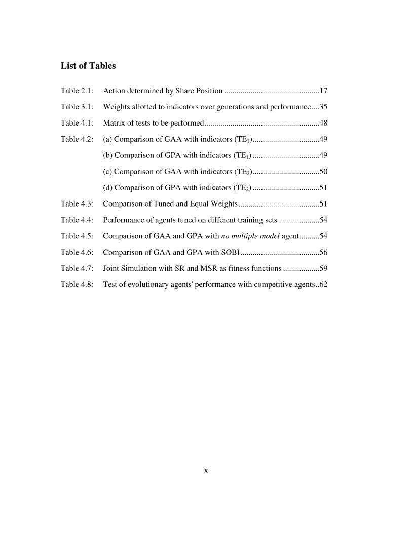
List of Tables
Table 2.1: Action determined by Share Position ...............................................17
Table 3.1: Weights allotted to indicators over generations and performance....35
Table 4.1: Matrix of tests to be performed.........................................................48
Table 4.2: (a) Comparison of GAA with indicators (TE1).................................49
(b) Comparison of GPA with indicators (TE1) .................................49
(c) Comparison of GAA with indicators (TE2).................................50
(d) Comparison of GPA with indicators (TE2) .................................51
Table 4.3: Comparison of Tuned and Equal Weights ........................................51
Table 4.4: Performance of agents tuned on different training sets ....................54
Table 4.5: Comparison of GAA and GPA with no multiple model agent..........54
Table 4.6: Comparison of GAA and GPA with SOBI.......................................56
Table 4.7: Joint Simulation with SR and MSR as fitness functions ..................59
Table 4.8: Test of evolutionary agents' performance with competitive agents..62
xi
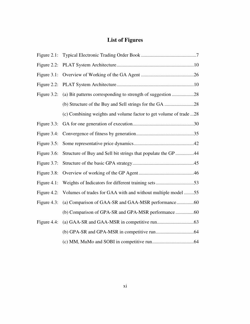
List of Figures
Figure 2.1: Typical Electronic Trading Order Book .............................................7
Figure 2.2: PLAT System Architecture...............................................................10
Figure 3.1: Overview of Working of the GA Agent ...........................................26
Figure 2.2: PLAT System Architecture...............................................................10
Figure 3.2: (a) Bit patterns corresponding to strength of suggestion ..................28
(b) Structure of the Buy and Sell strings for the GA ........................28
(c) Combining weights and volume factor to get volume of trade ...28
Figure 3.3: GA for one generation of execution..................................................30
Figure 3.4: Convergence of fitness by generation...............................................35
Figure 3.5: Some representative price dynamics.................................................42
Figure 3.6: Structure of Buy and Sell bit strings that populate the GP ...............44
Figure 3.7: Structure of the basic GPA strategy..................................................45
Figure 3.8: Overview of working of the GP Agent .............................................46
Figure 4.1: Weights of Indicators for different training sets ...............................53
Figure 4.2: Volumes of trades for GAA with and without multiple model ........55
Figure 4.3: (a) Comparison of GAA-SR and GAA-MSR performance..............60
(b) Comparison of GPA-SR and GPA-MSR performance ...............60
Figure 4.4: (a) GAA-SR and GAA-MSR in competitive run..............................63
(b) GPA-SR and GPA-MSR in competitive run...............................64
(c) MM, MuMo and SOBI in competitive run..................................64
1
Chapter 1. Introduction
The stock market represents an interesting dynamical system that intrigues
researchers from a number of disciplines including the machine learning community
which aims to build autonomous agents as part of a larger body of research into
autonomous agent systems [11]. Autonomous trading in stock markets is an area of
growing interest in the academic as well as commercial circles. Various attempts at
forecasting and prediction of time series data including neural network prediction
schemes have been moderately successful in the prediction of prices based on complex
mathematical models [12], [13]. While these are rigorous and expansive schemes to base
trading on, and despite their capability of producing good results when modeled right, the
fact remains that developing a sufficiently expansive model is a very difficult challenge.
As long as profitability is our primary concern, the goal remains to try and produce
productive and profitable strategies, even if they are specific to a market. We aim to
utilize existing intuition and combine ‘conventional wisdom’ with computational
techniques to try and improve profitability.
1.1 MOTIVATION
The stock market is a time varying, highly volatile process with so many factors
affecting its variation that it is very difficult to model its behavior with any precision.
Numerous investigations have been largely unsuccessful in predicting its behavior,
failing to produce substantial returns over basic, intuitive “reactionary” rules [14], [15].
In fact, a controversial but oft cited investment theory known as the Efficient Market
Hypothesis [16] implies that it is impossible to beat the market. In other words, it
suggests that the behavior of share price variation in the stock market does not contain
much predictable behavior that can be taken advantage of to ensure profitability. Other
studies also conclude that the autocorrelation for day to day changes is very low [17] and
that the process behaves very much like a random walk [18]. However, in the technical
trading community, the popular belief is that such an assumption would mean that
someone with no knowledge of the market making a random trade is about as likely to
2
succeed as an experienced trader. Deferring to intuition, they argue that this is not the
cases, and claim that there are some non-random aspects of the market that can be
exploited to trade profitably [6].
There is now substantial interest and possible incentive in developing automated
programs that would trade in this market much like a technical trader would, and have it
be relatively autonomous. Unless the market does not move at all during a trading day,
there is always some strategy that would work on a given day to make a lot of money.
These strategies would then lose money on other days, when a degenerate do nothing
strategy would have been a better way to go. We may think of a ‘successful strategy’ to
be one that maximizes the number of profitable days, as well as has positive average
profits over a substantial period of time, coupled with reasonably consistent behavior.
What does it mean to be ‘consistent’? And what is a substantial period of time? In the
context of our experiments in this thesis, we examine these questions in later sections.
Further discussion of evaluation criteria for our strategies can be found in Chapter 2. In
this thesis, we aim to study the effect of combining multiple ‘intuitive’ trading rules
within the framework of the Penn Lehman Automated Trading (PLAT) project [19].
There have been numerous studies on the use of technical trading strategies in intraday
stock trading. Even with exhaustive optimization of parameters, most of these strategies
have often proved too simplistic and coarse to utilize the variation of high frequency
stock price variation [20], [21].
A possible solution is to combine these individual strategies much like a human
trader would do on the floor of the stock exchange. Where the trader would rely on
combining intuition and experience to make a final decision, the strategy we wish to test
here is to emulate this behavior by using a genetic algorithm to tune the relative merits of
the individual rules. In this thesis, we aim to verify the validity of a scheme of operation
wherein the automated agent trades based on a combination of signals it receives from the
various ‘simplistic’ rules. We explore two schemes of combining rules – adding weights
to the various trading suggestions and adding or deleting certain rules altogether.
3
The two main contributions of this thesis are as follows. First, we propose that
technical indicators, although useful, are not as profitable when used alone, as they are
when used in conjunction with other technical trading rules. We explore two schemes of
combination of technical trading rules, using evolutionary algorithms (Genetic Algorithm
and Genetic Program) to optimize the combination of these rules, and conjecture that it
would work better than an ad-hoc combination. We develop agents with a weighted
majority design as well as one with provision for adding/deleting rules and the use of
Boolean operators as combining elements. Second, we look at improvements in fitness
functions for the evolutionary algorithms, so the model evolved by them are suited to
days of different price dynamics and increase profitability over days of all kinds of
behavior. To this end, we compare and contrast two different (but related) fitness
functions, and the performance of the resulting agents. Finally, we aim to present an
empirical study of performance of certain agent designs in controlled but fairly realistic
market simulations in an effort to explore possible vistas in profitable automated agent
development.
1.2 OUTLINE
The thesis aims to study the design, development and performance of an
automated trading strategy utilizing a composite technical trading strategy optimized by a
genetic algorithm. We also use a multiple model approach to control trading order
placement based on share position of the agent. Trading simulations and controlled
experiments are conducted to study the performance of this agent as well as its
components.
The rest of the thesis is organized as follows. Chapter 2 delves into some details
about the domain in which simulations are performed, background work and requisite
terminology. We also briefly touch upon the design of other agents we use in our tests.
Chapter 3 discusses the component technical trading strategies, as well as how they are
composed. A brief introduction to aspects of genetic algorithm and genetic programming

4
optimization used in our strategy, along with some implementation issues, are also
included. Chapter 4 contains a summary of experiment design, tests and simulations that
were performed as well as the results and includes an analysis of the results. Finally
Chapter 5 summarizes key results and a limitation of the work described in the thesis, and
discusses some ideas for future work in the area.
5
Chapter 2. Background and Related Work
2.1 BACKGROUND
In this section, we review some of the earlier work done by researchers in the
area. We also introduce basic trading concepts and discuss simulated trading
environments including the one used for experiments throughout this thesis.
2.1.1 Literature Survey
Stock markets have been around for centuries and the classic ‘scream’ across the
floor has been the medium of choice. Of late, however, markets have gone electronic.
NASDAQ is a distributed trading system completely run over networks of computers. It
allows customers' offers to be displayed on NASDAQ by their brokers or through ECNs
(Electronic Crossing Networks). ECNs such as Island [22] allow customers to display
their orders as well as trade orders with each other. Of course, trading in these markets on
an experimental basis is a costly exercise not only due to the transaction fees, but the
potential for steep penalties in the event of mistakes when a large amount of money is
risked. Additionally, experimentation to verify effects such as that of volume of trade on
profitability may involve high risks, as the downside to high volume trades is potentially
very high.
The factors described above warrant the use of trading simulators. These range
from in-class simulators, aimed at students to teach them the nuances of financial markets
[23], and financial simulators for exam preparation [24] to advanced market models like
the Santa Fe Artificial Stock Market [25]. However, various shortcomings of these and
other such simulators (like the failure to simulate a realistic market scenario and failure to
accommodate trading frequencies suitable to intra-day trading) have been addressed by
the PLAT domain. It uses real-world, real-time stock market data available over modern
ECNs and incorporates complete order book information; simulating the effects of
6
matching orders on the market. It also provides numerous APIs that allow the participants
to program their own strategies and trade with other agents as well as the external market.
Technical Analysis has a long history among investment professionals. However,
it has been approached with a great deal of skepticism in academia, over the past few
decades, largely due to the belief in the efficient market hypothesis. Though this field has
remained marginalized in literature, the accumulating evidence against the efficiency of
the market [21] has caused a resurgence of interest in the claims of technical analysis as
the belief that the distribution of price dynamics is totally random is now being
questioned. These techniques assume that, notwithstanding the efficient market
hypothesis, there exist patterns in stock returns and that they can be exploited by analysis
of the history of stock prices, returns and other key indicators. [6] provides details on
technical analysis for stock trading. Contained in [26] is a very good description of their
utility for our problem.
Initial attempts at isolating factors that affect trading yielded mixed results, but
when exploring a relatively new domain, negative or inconclusive results may still
contain valuable information. A multitude of day trading strategies from ‘resistance and
support’ [27] to the ‘market making with volume control’ [10(b)] strategy discuss volume
of trades (or the size of the buy or sell trading order in number of shares) as a parameter,
in the former case, to aid the decision process and in the latter, as a control mechanism.
Most studies however, have considered this a secondary factor and hence, literature on
studies of its exclusive effect on intraday trading is scarce. Order imbalance in volume
[10(c)] emerged as a useful volume parameter. Initial tests and an attempt at designing a
useful day trading strategy yielded useful information, despite some inconclusive results,
regarding the merits of order volume as a consideration when designing a trading
strategy.
There exists an immense body of work on the mathematical analysis of the
behavior of stock prices, stock markets and successful strategies for trading in these
7
environments. In recent years, the application of artificial intelligence (AI) techniques to
technical trading and finance has experienced significant growth. Neural networks [28]
have received the most attention in this regard and have shown various degrees of
success. The purpose of using neural networks is the ability to forecast data patterns that
are too complex for traditional statistical models. However, it is the lack of
interpretability of rules generated by a neural network that has caused a shift of interest in
favor of more transparent methods, and the genetic algorithm has risen in prominence as
an optimization tool in financial applications.
Many traders aim to practice technical analysis as systematically as possible
without automation while others use technical analysis as the basis for constructing
systems that automatically recommend trade positions. A good example of research
where attention is paid to system construction as opposed to rule construction is [29].
Other work in this area includes [28] who proposed using the method of genetic-based
global learning in a trading system. Here, genetic algorithms are used to attempt to find
the best combination indicators for prediction and trading. Results are shown to be
profitable but are reported in too little detail for objective scrutiny.
In [14], a financial currency exchange system that uses genetic algorithms to
optimize parameters for a simple technical trading indicator is described. This work has
considerable merit since intraday data are used. It is noted that the ultimate aim of such a
project would be to create a system based on an ensemble of indicators as we attempt. A
framework for systematic trading system construction and adaptation, based on genetic
programs was suggested in [30]. In [1], the use of genetic programming to discover
profitable trading rules was explored. A good introduction to genetic algorithms can be
found at [31]. Additionally, their use in investment strategies is described in [32].
Work in using a multiple model approach for development of an effective
intraday trading strategy [10a] and attempts at designing a strategy in the PLAT domain
using reinforcement learning and hill climbing as well as a market maker to be used in
8
competition in the PLAT domain have been explored to some extent [10b], but not in
conjunction with technical trading rules.
2.1.2 Relevant Trading Terminology
Before we discuss the environment and design involved in our work, we will
discuss the underlying mechanics of financial markets and exchanges, or the market
microstructure. In electronic markets such as NASDAQ, all orders are sent to the
exchange via an electronic interface and order-routing system. Since orders are cleared
electronically, the use of Electronic Crossing Networks (ECNs) has become prevalent.
One of the larger ECNs is Island [4].
Electronic Trading uses orders to buy or sell shares. These orders may be placed
at any price and any number of shares may be traded. Most commonly, we use market
and limit orders. A market order is an order to buy or sell shares at the current market
price. A limit order is an order to buy or sell a security at a specific price. In other words,
this kind of order is used to buy shares at a lower price than the current price or sell
shares at a higher price than the current. This kind of order does not guarantee a trade,
and such an order will be executed only if the current price happens to reach the quoted
price.
Most of the strategies described in this thesis use the limit order – and the terms
‘order’ and ‘limit order’ are used interchangeably in the following sections.
An order book is essentially a sorted list of orders placed by traders. The orders to sell
and buy are stored in the sell and buy order books respectively. Incoming (new) orders
are compared with corresponding orders in the opposite book – to check if it can be
executed immediately. If it can be executed, the corresponding order in the opposite book
is deleted to the extent to which it satisfies the order. If the incoming order is large, then
more than one order in the opposite book may be executed to satisfy the need. Incoming
orders that are not immediately executed (partly or fully) are entered into the appropriate
9
order book in an appropriate position ranked by price and time of order placement (in
case of a tie).
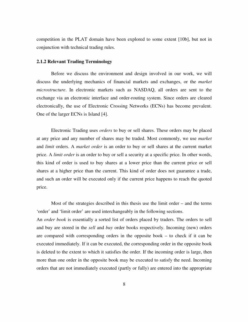
Figure 2.1: A typical electronic trading order book
Order book imbalance is the difference in price or volume of trades between the sell and
buy order books. Volume of trades is usually expressed as number of shares associated
with orders. Programs written by stock traders/organizations with the specific intent of
placing trading orders, according to an algorithm is defined as an agent in the following
sections. These agents monitor price variation, and based on the programmed algorithm,
place orders. Of course, various levels of autonomy can be assigned to the process.
Human intervention can be enforced to a high level – wherein the human trader uses the
algorithm purely as an indicator or recommendation, and on the other hand, the agent
may have more autonomy and is allowed to automatically place bids on behalf of the
trader. In this thesis, and all the following sections, we program strategies (that monitor
current market statistics, and based on the algorithm, decide the action to be taken) that
the agent uses to perform certain trading actions.
10
2.1.3 Stock Market Simulators
Automatic trading has been an active area of research over the last decade, and a
primary requirement to this cause is a realistic simulation of the market – owing to the
high expenses associated with experimenting on the actual market. This has led to the
development of numerous simulators (virtual markets). These simulators have been
designed from various perspectives – from the study of market mechanism to classroom
teaching of finance fundamentals. The Santa Fe Artificial Stock market project is an
example of the former and [20], the latter. The Stock Market Game [33] is a simulator
where participants can study the tradeoffs in risks and rewards in making decisions
according to certain strategies. Another simulator that can be used by traders to
experiment on managing different portfolios is the Virtual Stock Exchange [34].
However most of these simulators create whole new stock exchanges, independent of the
real world trades.
The bids placed by the agent needs to affect the economy of the market it trades
in. So, in any scenario where virtual bids are placed at current prices over a period of
time and evaluated in a real world economy, the economy is not affected by any action of
the agent. All the above shortcomings in various stock market simulators motivated the
research of the Penn-Lehman Automated Trading (PLAT) group. The PLAT simulator
seamlessly combines the virtual orders from participating virtual trading agents with
orders in a real world ECN, to create an environment very close to the real world. The
Penn Exchange Server (PXS), a component of the PLAT project , is a platform for
developing novel, principled automated trading strategies. The real-data, real-time nature
of PXS lets us examine computationally intensive, high frequency, possibly high-volume
trading strategies.
2.1.4 PLAT Domain
The Penn Lehman Automated Trading (PLAT) domain uses the Penn Exchange
Server (PXS) to which the trading agents can plug in. PXS uses real-world, real-time
11
stock market data for simulated automated trading. It frequently queries the Island
electronic crossing network’s (ECN) web-site to get the most recent stock prices and buy
and sell order books. A detailed discussion of the working of PXS can be found in [19].
PXS works in a manner very similar to a regular ECN. The order books maintained by
the PXS server are a combination of real orders and virtual orders (placed by the agents
that are plugged into it). Real orders correspond to those on the Island ECN. At every
processing cycle, an attempt is made to match virtual orders. All possible transactions are
processed, following which, an attempt is made to match the virtual orders with real
orders. After this is over, all remaining unmatched orders (virtual and real) are combined
to form a single pair of buy and sell order books. The simulator also computes the profit
and losses of each connected trading agent in real time, and displays it in an output file.
PXS is equipped for testing strategies on historical data and also for running in the
live mode, starting and ending at the same time with normal trading sessions of the
NASDAQ. The simulator supports limit orders only. The trading strategies connected to
the server, which we have until now referred to as an agent will now be used
interchangeably with client for the rest of this work. In the simulation, the best ask price
is the lowest price any seller (either trading agents or outside market customers) has
declared that they are willing to accept; the best bid price is the highest price any buyer
has declared that they are willing to pay. If a new buy order has bid price greater than or
equal to the best ask price or a new sell order has ask price less than or equal to the best
bid price, the order will be matched in the amount of the maximum available shares and
the trade is executed. If a bid price is higher than the ask price, the trading price is the
average of these two (bid and ask) prices. If orders cannot be matched immediately, they
are kept in the queue to wait for possible future matches.
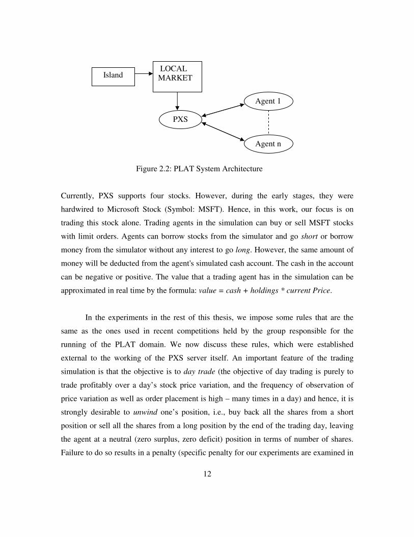
12
Figure 2.2: PLAT System Architecture
Currently, PXS supports four stocks. However, during the early stages, they were
hardwired to Microsoft Stock (Symbol: MSFT). Hence, in this work, our focus is on
trading this stock alone. Trading agents in the simulation can buy or sell MSFT stocks
with limit orders. Agents can borrow stocks from the simulator and go short or borrow
money from the simulator without any interest to go long. However, the same amount of
money will be deducted from the agent's simulated cash account. The cash in the account
can be negative or positive. The value that a trading agent has in the simulation can be
approximated in real time by the formula: value = cash + holdings * current Price.
In the experiments in the rest of this thesis, we impose some rules that are the
same as the ones used in recent competitions held by the group responsible for the
running of the PLAT domain. We now discuss these rules, which were established
external to the working of the PXS server itself. An important feature of the trading
simulation is that the objective is to day trade (the objective of day trading is purely to
trade profitably over a day’s stock price variation, and the frequency of observation of
price variation as well as order placement is high – many times in a day) and hence, it is
strongly desirable to unwind one’s position, i.e., buy back all the shares from a short
position or sell all the shares from a long position by the end of the trading day, leaving
the agent at a neutral (zero surplus, zero deficit) position in terms of number of shares.
Failure to do so results in a penalty (specific penalty for our experiments are examined in
LOCAL MARKET
PXS
Agent 1
Agent n
Island
13
later sections). Any excess shares held at the end of the day are valued at zero. Shares
that are short need to be bought back by the agent at twice the closing price.
Other factors to be accounted for are the fact that trading happens continuously
and in real time. The agent strategy cannot be externally changed in the middle of a
trading day. Also, PXS has provisions to accommodate transaction costs, much like the
real market. Each time a trade is executed by PXS, one side of the order exists in one of
the order books already, and the other side of the order is the incoming order. In order to
reward an agent for providing liquidity (providing the books with unfulfilled orders to
match potential orders from the other side of the book), the agent that has its order in the
book already – is rewarded with a rebate. The agent with the incoming order
correspondingly is charged a fee – as it eliminates liquidity from the order books. The
daily return is thus defined as:
Daily Return = Cash – Unwinding Penalty – Transaction fees + Trading Rebates
The transaction fees charged for trade, in the experiments in this thesis, follows exactly
the pricing mechanism of the Island ECN. For each trade executed by PXS, the agent
whose order was already in the books receives a REBATE of $0.002, and the agent who
placed the incoming order (that was executed immediately) pays a transaction FEE of
$0.003. This way, agents are rewarded for maintaining liquidity on the server and
penalized for depleting the liquidity. Within the framework defined so far, the objective
of the agent strategy is to maximize profits. Specifically, the expected return, measured
by the Sharpe ratio, is to be maximized (section 2.4). There are competing objectives at
play here. The need to maximize profits implies that an extreme position be taken by
trading as much as possible when an opportunity for profit is seen. On the other hand, the
need to unwind one’s position at the end of the day as well as the strict statistical measure
of performance suggests a more cautious approach. There are no limits to how many
shares an agent may buy or sell in a day, or how many shares an agent may hold (or have
a deficit of) at any given point of the day. So there is room for exploration of strategies.
Unreasonable positions are avoided by most agents due to the focus on liquidity, but
14
counter-intuitive, extreme strategies are accommodated within this framework.
A key point to note is that it is desirable to make consistent small profits over
many days, as opposed to adopting strategies that provide high returns but result in high
variance, thereby neutralizing the profits and resulting in a small Sharpe ratio. The need
for a controlled trading strategy is evident.
2.2 EARLY AGENT DESIGN AND THE NEED FOR A COMPOSITE STRATEGY
Some financial and commodity market traders study market price history with a
view to predicting future price changes in order to enhance trading profitability. This
study is called technical analysis. Technical trading rules involve the use of technical
analysis to design indicators that help a trader determine if current behavior is indicative
of a particular trend, as well as the timing of a potential future trade. Owing to the
difficulty of managing complex models of the market and using rigorous, adaptive
decision techniques, day traders tend to use simpler and more intuitive decision rules.
This ‘common sense’ approach has often proven quite effective [10a] and has been
considered a good candidate for automation [35].
The hypothesis is that a robust strategy can be designed by composing multiple
‘intuitive’ strategies. Robustness and relatively complex behaviors can be achieved by
synthesizing multiple, intuitive strategies. Basic stock trading is commonly perceived to
be governed by the dictum ‘buy low, sell high’. If an agent were to buy a share at a low
price and sell it at a higher price, then a profit of high price – low price has been made.
Numerous such trades over the day would accumulate profit for the trader. A problem in
stock markets is that the future is unknown and it is therefore unclear if a decision to buy
or sell in anticipation of a favorable movement in the future would yield profit. This
decision is further complicated by the strict need to unwind, as is the case in intraday
(high frequency) trading. The aim is to leverage the small price changes to one’s
advantage. A process of unwinding, i.e. the process of selling excessive shares if in
excess and buying the number of shares required to make up the deficit, when short, is

15
implemented in the experiments in the following sections. (The case of possible retention
of a short or long position overnight, is a different body of research, and includes factors
such as overnight information, adjusted prices, etc).
Synthesis of multiple rules to come up with a composite trading strategy has been
tried before in various forms – with the component rules being everything from complete
rules [36] to very basic predicates and operators that are combined to generate complex
rules [37]. In this work, we aim to synthesize a strategy where the component rules are
independent strategies in themselves, so they would appeal to a human trader. It would be
hard to intuitively see the utility of a rule that was a long series of conjunctions and
disjunctions of basic predicates. So, we aim to see if existing, simple, intuitive strategies
can be composed in some way to make a robust, profitable strategy. In the following
subsections, we will briefly discuss some of the strategies that have been implemented
and tested in the PLAT domain, with emphasis on the ones we will use as competitive
agents in experiments in later sections.
2.2.1 Static Order Book Imbalance (SOBI) Strategy
The SOBI [10d] strategy bases its decision on the differences in the distribution of
volume at different prices in the BUY and SELLS order books.
Let bi (i = 1, 2, 3, 4) represent the volume-weighted average price (VWAP) of the top
i*25% of the volume in the buy order book. For instance, b1 is computed by taking the
top 25% of the buy order volume, and computing the average price offered per share.
Similarly, let si (i=1,2,3,4) be the volume-weighted average price of the top i*25% of the
volume in the sell order book. Also, let lastPrice be the most recently updated market
price.
Si: si – lastPrice
Bi: lastPrice - bi
Note that Si and Bi will always be positive numbers.
16
They can be interpreted as a measure of the "distance" from the last price of the top
i*25% of the respective order book. The strategy computes the VWAP of the PXS BUY
and SELL order books, and compares them to the PXS last price.
The basic idea is that the the difference between the respective VWAPs and the
last price is an indicator of the level of support that the buyers and sellers show. For
example, if the VWAP of the buy book is much further from the last price than the
VWAP of the sell book, it is a sign that buyers are less supportive of this price than are
sellers, as indicated by their limit orders (statistically) standing further off. In this case,
SOBI will place an order to sell shares, on the theory that the weaker buy-side support
will cause the price to fall.
To summarize, the SOBI strategy, at every tick, computes Si and Bi and places
buy or sell orders according to the following rules:
If (Si - Bi > theta), place an order to buy volume(v) shares at (price);
If (Bi - Si > theta), place an order to sell volume(v) shares at (price);
theta being a controlled parameter.
2.2.2 Market Maker
A market maker buys stock when the price is increasing at an increasing rate and
sells stock when the price is decreasing at an increasing rate. However, rather than wait
for a trend reversal to unwind the accumulated share position, the agent always places
buy and sell orders in pairs. When the price is increasing at an increasing rate, the agent
places a buy order at price p (based on the order book) and immediately places a sell
order at price p + �, with the confidence that the latter will be matched shortly when the
price has gone up enough. The situation is assumed to be symmetric when the price is
decreasing at an increasing rate. For further discussion, the reader is pointed to [38]. In
our tests, this (having been a successful agent in past competitive tests) is used as a
competing agent.
17
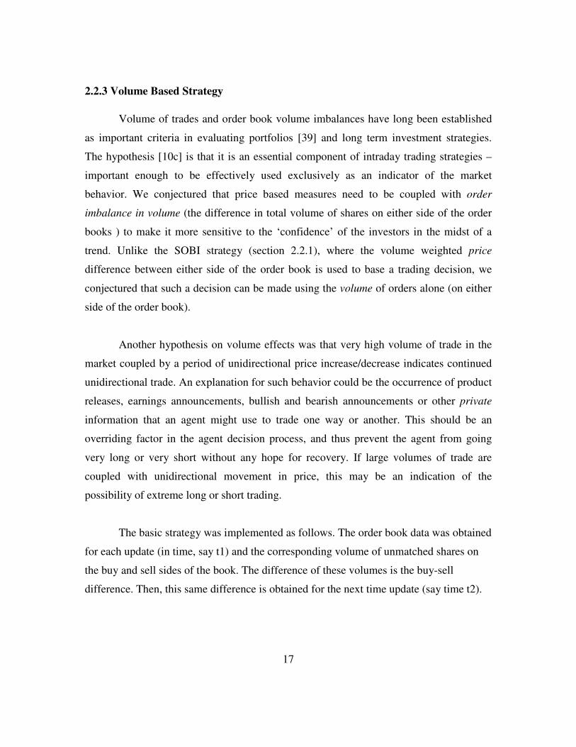
2.2.3 Volume Based Strategy
Volume of trades and order book volume imbalances have long been established
as important criteria in evaluating portfolios [39] and long term investment strategies.
The hypothesis [10c] is that it is an essential component of intraday trading strategies –
important enough to be effectively used exclusively as an indicator of the market
behavior. We conjectured that price based measures need to be coupled with order
imbalance in volume (the difference in total volume of shares on either side of the order
books ) to make it more sensitive to the ‘confidence’ of the investors in the midst of a
trend. Unlike the SOBI strategy (section 2.2.1), where the volume weighted price
difference between either side of the order book is used to base a trading decision, we
conjectured that such a decision can be made using the volume of orders alone (on either
side of the order book).
Another hypothesis on volume effects was that very high volume of trade in the
market coupled by a period of unidirectional price increase/decrease indicates continued
unidirectional trade. An explanation for such behavior could be the occurrence of product
releases, earnings announcements, bullish and bearish announcements or other private
information that an agent might use to trade one way or another. This should be an
overriding factor in the agent decision process, and thus prevent the agent from going
very long or very short without any hope for recovery. If large volumes of trade are
coupled with unidirectional movement in price, this may be an indication of the
possibility of extreme long or short trading.
The basic strategy was implemented as follows. The order book data was obtained
for each update (in time, say t1) and the corresponding volume of unmatched shares on
the buy and sell sides of the book. The difference of these volumes is the buy-sell
difference. Then, this same difference is obtained for the next time update (say time t2).
18
The decision rule is stated as:
If (buy – sell)t2 > (buy – sell)t1
buyOrder(buyprice, ordervolume);
Else If (buy – sell)t1 > (buy – sell)t2
sellOrder(sellprice, ordervolume);
Else do nothing
The volume of orders was tuned with an optimization algorithm that maximized the
function:
]21**2[)])}(*()*[{( volvolpriceteordervolumbuypriceeordervolumsellprice �−�−−�
where vol1 and vol2 are the buy and sell volumes respectively.
As discussed earlier, in the event that high trading volumes accompanied unidirectional
price movement, a cautionary approach was taken and implemented as:
check totalvolume
if (totalvolume is very high)
for (3 time steps)
if (price increases for three time steps)
buyvolume = sellvolume = 0 ;
else if (price decreases for three time steps)
buyvolume = sellvolume = 0 ;
Else do basic strategy
Although crude, this guard mechanism proved quite useful.All of these early attempts at
designing strategies seemed to indicate the need for combining many simple intuitive
strategies, as well as using a more efficient control mechanism to take care of cash and
share position.
2.2.4 Multiple Model Strategy
This approach was developed and implemented by Ramamoorthy [10(a)] as part
of a project for a class and was a successful agent in competitive simulations in April
2004 (Appendix 3). The intuition behind this strategy is that there are periods of time
when the behavior of the stock return is, in fact, mean reverting and a simple strategy

19
with this assumption would, in a statistical sense, produce profits. When the markets
deviate from this favorable model, the resulting effect would be observed from
instantaneous cash and stock holdings. This could be used to trigger a mode switch to a
different strategy that does not assume the mean-reverting nature of stock prices. In the
case of the agents we aim to implement in our thesis, we incorporate this strategy (as is,
with a few very minor modifications) in conjunction with our algorithms, as a control
measure. Intuitively, we can think of this as a faucet that we turn to control various rated
of flow. If we think of the trading suggestion and suggested trading volume as the
suggested trading parameters, then it is regulated by the action mode (safe or regular)
suggested by the multiple model mechanism, which we describe [from 10(a)] below.
The problem of detecting the agent and the market’s mode can be approached by
thinking in terms of two key variables – cash held by the agent and net shares held by the
agent. This representation can be visualized as a two dimensional state space, the axes
being cash axis and share axis respectively. The idea is to move in the positive direction
on the Cash axis while trying to stay close to zero on the Share axis. The effect of the
market is to move the agent’s current position along the Cash axis towards the negative
side. The agent, on its part, can issue commands to move along the Share axis.
Occasionally, the agent’s state is far from the Share axis.
So, the idea is to explicitly control risk and rewards by tuning the one variable
available to the agent, the share holdings, in response to observed variables, the last price.
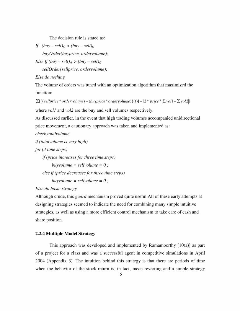
The allowed modes of trading the agent can follow are:
Regular: Perform trading as usual.
Safe: Try to divest holdings when profitable, otherwise, do nothing. This would never
increase holdings in the unfavorable direction (in the state space).
Risk Seeking: Trade with lower margins and larger volumes in expectation of higher
returns.
20
These behaviors can be composed as shown in the table below:
Cash
Share
Very
Negative
Negative Zero Positive Very Positive
Very Short Safe Safe Safe Safe Safe
Short Safe Safe Regular Regular Safe
Zero Safe Regular Regular Regular Risk Seeking
Long Safe Regular Regular Risk Seeking Risk Seeking
Very Long Safe Safe Safe Safe Safe
Table 2.1: Mapping position in cash-share space to a mode of action
2.2.5 Other Strategies
Numerous other strategies have been implemented in the PLAT domain and
implemented in competitive runs, with varying degrees of success. Among the more
successful of these agent strategies, is the Reverse Strategy [48]. This strategy runs
counter to the traditional dictum of “sell when the price is falling and buy when it is
rising”. It buys when the price is dropping and sells when the price is rising. Other
techniques explored use trader message boards and gleaning information from the news
online [51]. In the following sections in this chapter, we briefly discuss evolutionary
algorithms and trading evaluation criteria with relevance to the central strategy discussed
in this thesis.
2.3 GENETIC ALGORITHMS AND GENETIC PROGRAMMING
The areas of artificial intelligence and its application to technical trading and
finance have seen a significant growth in interest over the past few years. Specifically,
the use of evolutionary methods such as genetic algorithms (GA) and genetic
programming (GP) in this domain has been examined. These approaches have found
financial applications in options pricing [40] and as an optimization tool in technical
trading applications [30].
21
Evolutionary learning algorithms derive inspiration from Darwinian evolution. GAs are
population-based optimization algorithms and the first proposal of this idea has been
credited to Holland [41]. They have since found applications in a wide range of problems.
GPs are an extension of this idea proposed by Koza [42] with a view to evolving
computer programs.
GAs are iterative systems and aim to find near optimal solutions. They differ from
standard search algorithms in that they use a population of possible solutions rather than
tuning a single one. Although convergence to the global optimum is not guaranteed, they
are quite robust in producing near optimal solutions to a wide range of problems and, in
particular, those that are not easily reducible to a precise mathematical formulation. In
pseudo code below, a basic genetic algorithm (a formulation we stick to reasonably
accurately) is described.
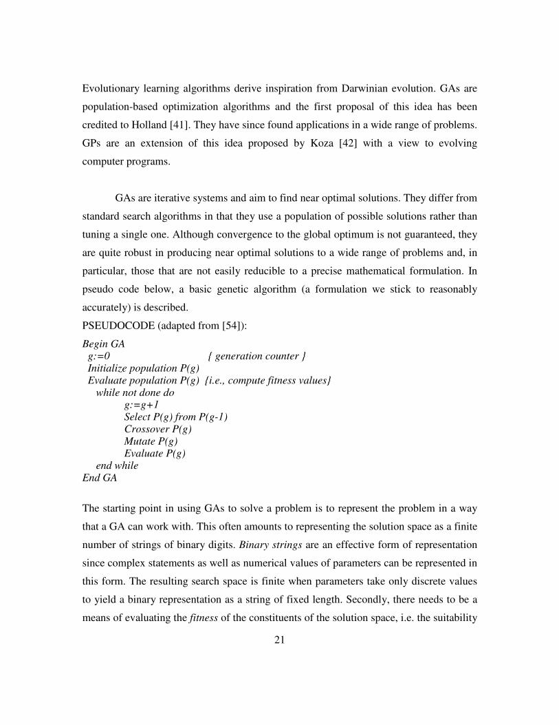
PSEUDOCODE (adapted from [54]):
Begin GA g:=0 { generation counter } Initialize population P(g) Evaluate population P(g) {i.e., compute fitness values} while not done do g:=g+1 Select P(g) from P(g-1) Crossover P(g) Mutate P(g) Evaluate P(g) end while End GA
The starting point in using GAs to solve a problem is to represent the problem in a way
that a GA can work with. This often amounts to representing the solution space as a finite
number of strings of binary digits. Binary strings are an effective form of representation
since complex statements as well as numerical values of parameters can be represented in
this form. The resulting search space is finite when parameters take only discrete values
to yield a binary representation as a string of fixed length. Secondly, there needs to be a
means of evaluating the fitness of the constituents of the solution space, i.e. the suitability
22
of each potential solution, for how well they perform. For example, in the case of
selecting trading rules the fitness could be viewed as the profitability of the rule tested
over a time series of historical price data, or a function of this variable.
Genetic Programs are a variation of the standard genetic algorithm, wherein string
lengths may vary within the solution space. Unlike in GAs, solutions in GP can be seen
as non-recombining decision trees [43] with non-terminal nodes as functions and the root
as the function output. These are usually the optimization algorithm of choice in cases of
evolving strategies based on Boolean operators – when the solution may be evolved with
varying depth in the tree [44]. It is inherently more flexible than the GA, but care needs
to be taken in representation to avoid over-fitting (the phenomenon where a classifier is
trained too minutely to fit the training data – causing diminished performance on data
outside of the training sample, also called out-of-sample data).
2.4 PERFORMANCE CRITERIA
A class of performance criteria commonly used in the financial community are
measures of risk-adjusted investment returns. Risk-adjusted returns are a measure of the
returns of an asset adjusted for risk or volatility. In other words, consistency is rewarded
and volatile trading patterns are not. Common measures within this class are the Sharpe
and Modified Sortino ratios.
2.4.1 Sharpe Ratio
Probably the most popular measure of performance of asset trading in finance is
the Sharpe ratio, introduced by William Sharpe [45], and originally introduced to
measure the performance of mutual funds. Essentially, it is excess return divided by risk
as measured by the standard deviation of return. For the rest of the thesis, we will assume
that ‘return’ is ‘daily return’. We recall from section 2.1.4 that daily return, for our
experiments, is defined as:
Daily Return = Cash – Unwinding Penalty – Transaction fees + Trading Rebates

23
If the average daily return (defined as the amount of money made after money spent and
sale of remaining stocks are adjusted for, at the end of the trading day) is supposed to be
Ri then the average daily return is:
�=
=N
iiR
NR
1
1
The standard deviation of returns is,
)(2/1
1
2
11
��
���
� −−
= �=
N
ii RR
Nσ
Thus, the Sharpe ratio is,
Sharpe ratio = σR
2.4.2 Modified Sortino Ratio
Despite the common use of Sharpe ratio in the field of financial performance
evaluation, quite often, traders are often not perturbed by the possibility of volatile return
structure provided the strategy is mostly profitable. Sortino ratio, introduced in the early
1980’s, is a modification of the Sharpe ratio that differentiates ‘harmful volatility’ from
volatility in general, using a value for downside deviation only. While it has limited basis
in theoretical study in the area [46], we hypothesize that it warrants a closer look,
especially in the domain of intraday trading agent performance evaluation.
The Sortino ratio, as defined in [46], is a more complex model - suitable for
rigorous statistical evaluation of asset returns – than we aim to use in the experiments of
our thesis. A usable form of this ratio, which we will use in following sections, is:
Modified Sortino Ratio = neg
Rσ
where negσ is the standard deviation of negative returns only (over the given period of
time). R represents the returns (as described in section 2.4.1).
24
2.5 THE DATA
The PLAT domain is an experimental test bed that is configured to run with the
historical as well as live mode data. The data comes from a mirror of the Island ECN
which trades NASDAQ stock. The only stock used here is the Microsoft (Symbol:
MSFT) stock. The stock data consists of a bid and an ask price table, that lists in order of
preference, the respective orders placed by agents/traders. The difference between the
topmost entries of this table is called the spread. A number of past trading days’ books
are stored in the PLAT project. The process of selection of data (trading days) used for
training and testing is as follows. There were days from early December 2003 to mid July
(archived in the PLAT project for MSFT) that we used as a baseline set of data for
consideration for our thesis. Over half of these days were eliminated due to incomplete
data over the day or corruption of data. Of the remaining days, attempts were made to
make sure the data included data representative of a number of different stock behaviors
over a training day. Specifically, we made a list of all the days in the archives, which we
deemed as tradable after weeding out incomplete data, and this list was checked with a
list of trading data we obtained from Yahoo! Finance pages [52]. The data, based on
details such as opening price, closing price, high and low prices of the day, was divided
into various categories such as increasing, decreasing, mean reverting, etc. Further
discussion on the classification of days based on price dynamics is included in
Appendices 1 and 2. Our final list included 60 days. Of these, 15 days were set aside for
our competitive tests with previously successful agents. The remaining days were split up
into training and test days, and we made sure that no experiment had any overlap between
its training and test set of days.
25
Chapter 3. Agent Design
In this chapter, we will discuss design issues, and the techniques used in
development of agents for trading in PLAT domain. Our primary aim is to design trading
strategies that resemble a technical trader who would systematically, and based on a set
of pre-specified evaluation criteria; choose a subset of trading strategies from a larger set
of trading rules, and evaluate the performance of these strategies in various competitive
scenarios. The basic idea is to combine popular, ‘intuitive’ technical analysis indicators
and rules to profitably trade in the PLAT domain. Trading strategies and rules are
allowed to combine in two different mechanisms – with the use of genetic algorithms and
genetic programs – to evolve strategies that are aimed to be profitable, and perform well,
under the different evaluation criteria involved.
3.1 GENETIC ALGORITHM AGENT (GAA)
In an attempt to make a profitable, robust strategy using simple intuitive laws that
appeal to the human trader, we use multiple technical trading rules in a weighted
combination to produce a unified strategy. In addition to designing an automated strategy
that is intuitively appealing, the generation of effective strategies using complete,
comprehensible indicator strategies may help in the understanding of these component
strategies, their effects and limitations.
In this formulation, we use a number of basic (indicator) strategies in a weighted
combination to produce a cumulative trading action at every tick (a tick in the following
sections is the point in a trading day when the books are updated and fresh data is
available). The algorithm uses principles from the weighted majority algorithm [47] in
the use of suggestions from the component strategies and combining them using a
weighted majority. We propose the use of a similar suggestion or voting mechanism
wherein each indicator would signal a buy, sell or do nothing action. We recall that the
steps involved in trading in this environment include getting the raw order book data,
evaluation of a recommended action by each of the indicator strategies and combining
these indicators using the respective weights giving us a cumulative suggestion (a
26
weighted majority). This is followed by a multiple model control mechanism that
determines the mode it should trade in (A discussion of modes of trading is in section
2.2.4). Earlier, we compared the control mechanism to a faucet, acting as the final
regulator on the trading decision and volume suggested by the composite strategy so far.
It has the power to veto a trading decision suggested by the composite algorithms, when
in the safe mode or allow the trade to continue unaltered in the regular mode.
The multiple model control mechanism determines the trading mode based on
current holdings of the agent (also called the share position). The share position is the
number of shares that the agent has accumulated (long position), or the number of shares
that is deficient (short position), over the trading day up to that point. It is not difficult to
imagine that a human trader would behave differently when in an extremely long or short
position (risk averse) as opposed to when he is in a relatively neutral share position (risk
neutral or risk seeking). A similar behavior is desired from an autonomous automated
agent in determining the trading action to be taken. The agent evaluates its current share
position and this helps keep the agent from following a possibly unidirectional market
trend to the end of the day, and reaching a very long or short position. In essence, this
mechanism is a control measure to ensure the agent achieves a share position as close to
neutral (zero accumulation or deficit) as possible. In section 2.1.4, we discussed that
unwinding is an important constraint and enforced external to the mechanism of PXS.
With the use of Sharpe and Sortino ratios, the imposition of this rule makes sense in that
it provides for a uniform set of statistics to evaluate trading agents on. We achieve the
objective of unwinding with the use of a multiple model mechanism. One of the changes
in our implementation, when compared to that in section 2.2.4, is that we have eliminated
the use of the ‘risk-seeking’ mode of operation. The reasoning behind this decision is that
such a behavior is proposed only for extremely high cash as well as share positions. This
is not only a highly unlikely occurrence, but also a situation where we hypothesize a
regular behavior should suffice in recovering a reasonable share position – keeping in
mind the relatively robust design of the market evaluation phase of the strategy. This
multiple model scheme examines the agent’s share position and provides a mode of
27
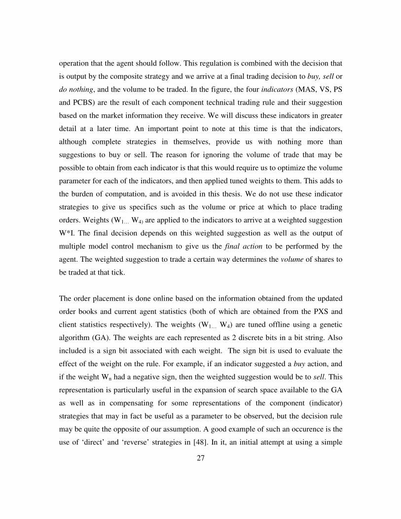
operation that the agent should follow. This regulation is combined with the decision that
is output by the composite strategy and we arrive at a final trading decision to buy, sell or
do nothing, and the volume to be traded. In the figure, the four indicators (MAS, VS, PS
and PCBS) are the result of each component technical trading rule and their suggestion
based on the market information they receive. We will discuss these indicators in greater
detail at a later time. An important point to note at this time is that the indicators,
although complete strategies in themselves, provide us with nothing more than
suggestions to buy or sell. The reason for ignoring the volume of trade that may be
possible to obtain from each indicator is that this would require us to optimize the volume
parameter for each of the indicators, and then applied tuned weights to them. This adds to
the burden of computation, and is avoided in this thesis. We do not use these indicator
strategies to give us specifics such as the volume or price at which to place trading
orders. Weights (W1… W4) are applied to the indicators to arrive at a weighted suggestion
W*I. The final decision depends on this weighted suggestion as well as the output of
multiple model control mechanism to give us the final action to be performed by the
agent. The weighted suggestion to trade a certain way determines the volume of shares to
be traded at that tick.
The order placement is done online based on the information obtained from the updated
order books and current agent statistics (both of which are obtained from the PXS and
client statistics respectively). The weights (W1… W4) are tuned offline using a genetic
algorithm (GA). The weights are each represented as 2 discrete bits in a bit string. Also
included is a sign bit associated with each weight. The sign bit is used to evaluate the
effect of the weight on the rule. For example, if an indicator suggested a buy action, and
if the weight Wn had a negative sign, then the weighted suggestion would be to sell. This
representation is particularly useful in the expansion of search space available to the GA
as well as in compensating for some representations of the component (indicator)
strategies that may in fact be useful as a parameter to be observed, but the decision rule
may be quite the opposite of our assumption. A good example of such an occurence is the
use of ‘direct’ and ‘reverse’ strategies in [48]. In it, an initial attempt at using a simple
28
decision rule based on current and previous price used a buy action when the price
increased and sell action when the price deceased. However, when they switched the
actions to use a sell action for increasing price and a buy action for an increasing price, it
yielded superior performance. Such occurrences would be compensated for with the use
of the sign bit in our bit string as the GA is expected to tune itself for better performance.
Figure 3.1: Overview of working of the GA agent
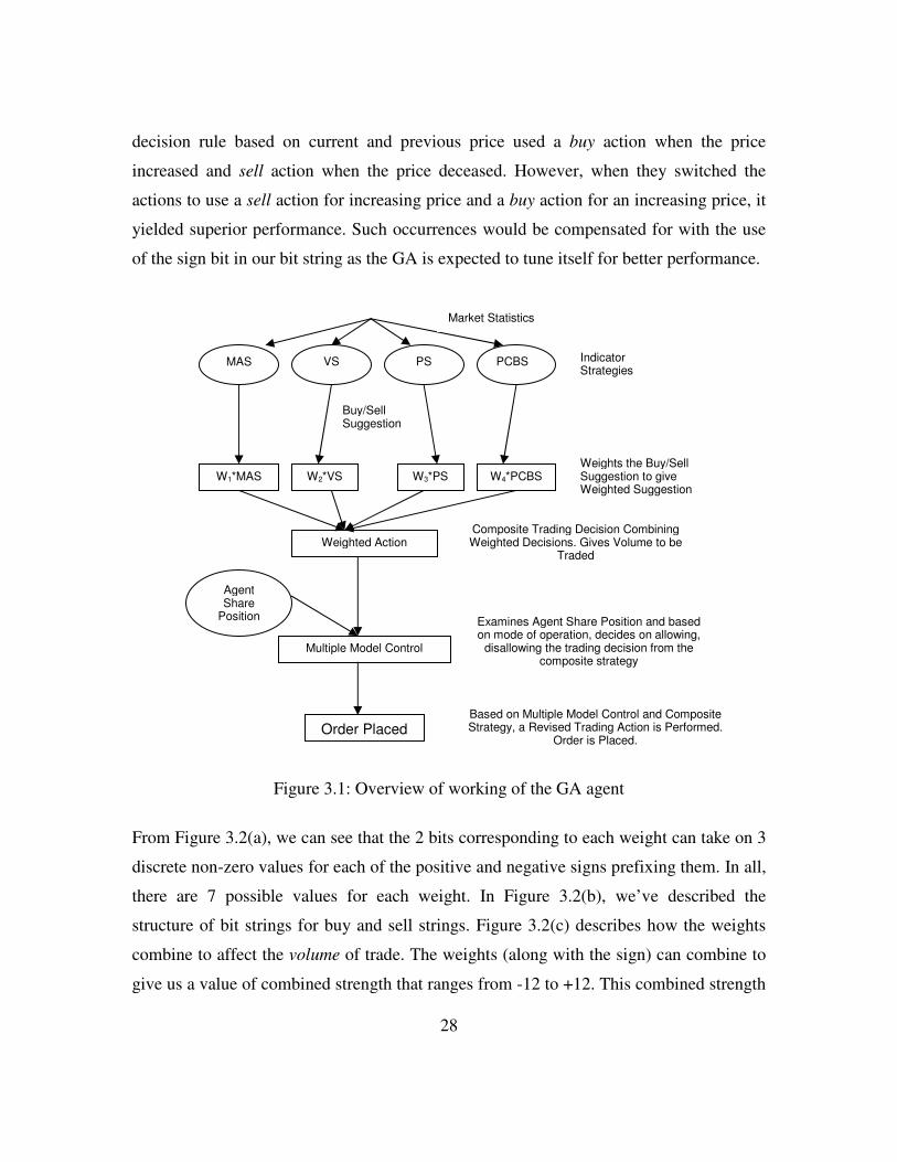
From Figure 3.2(a), we can see that the 2 bits corresponding to each weight can take on 3
discrete non-zero values for each of the positive and negative signs prefixing them. In all,
there are 7 possible values for each weight. In Figure 3.2(b), we’ve described the
structure of bit strings for buy and sell strings. Figure 3.2(c) describes how the weights
combine to affect the volume of trade. The weights (along with the sign) can combine to
give us a value of combined strength that ranges from -12 to +12. This combined strength
MAS VS
PS
PCBS
W1*MAS W2*VS W3*PS W4*PCBS
Buy/Sell Suggestion
Market Statistics
Indicator Strategies
Weights the Buy/Sell Suggestion to give Weighted Suggestion
Weighted Action
Composite Trading Decision Combining Weighted Decisions. Gives Volume to be
Traded
Multiple Model Control
Agent Share
Position Examines Agent Share Position and based on mode of operation, decides on allowing,
disallowing the trading decision from the composite strategy
Order Placed Based on Multiple Model Control and Composite Strategy, a Revised Trading Action is Performed.
Order is Placed.

29
value is then multiplied with a constant volume factor (the value of this was fixed
empirically at 25 throughout this thesis) to give us the volume of shares to be traded at
that particular tick.
Figure 3.2 (a) Correspondence of bit patterns of weights to strength of suggestion
SIGN W1 SIGN W2 SIGN W3 SIGN W4 BUY 0 01 1 11 0 00 0 10
SIGN W1 SIGN W2 SIGN W3 SIGN W4 SELL 0 00 1 10 0 01 0 01
Figure 3.2 (b) Structure of the buy and sell bit strings that populate the GA
Figure 3.2 (c) Combining weights and volume factor to get volume of trade
Bit Pattern Strength of Suggestion
00 0 (No trade)
01 1 (Weak)
10 2 (Strong)
11 3 (Very Strong)
Combining Weights
W1 W2 W3 W4
-11 + -11 + -11 + -11
00 + 00 + 00 + 00
11 + 11 + 11 + 11
-12
0
12
Volume Factor
The combination of weights is multiplied to
the volume factor to give final volume to be traded
Volume of Trade

30
The length of the bit strings are limited to 12 bits (2 bits and a sign bit for each indicator),
due to the burden of computation time. The reasoning was that longer strings would make
the search space of possible solutions much larger (owing to the increased number of
unique combination of bits. The computation time of the GA, in its current format,
already runs into more than a day, as each generation is essentially a simulation over a
trading set (15 days run in historical mode) with multiple agents (in this case 20 per
generation). The time taken to run the simulation also increases with the number of
agents plugged in simultaneously. It is evident that an increase in the number of
individual bit strings per generation would be required to search a reasonable portion of
the search space, in case the number of bits per string was increased. This would
consequently lead to increase in computation time, and training would become a very
computationally intensive task. To avoid this predicament, we limited the bit strings to 12
bits, at the cost of increased granularity in weight values.
In preliminary work done in a class, we hypothesized that technical trading
indicators are sometimes not symmetrical. The market, as an aggregate, swings upward
or downward from an opposite trend – and these effects, when viewed on a chart, are
called shoulders. These shoulders may be wider when a downward trend ends and
narrower when an upward trend ends, or vice versa, depending on the setup of the
decision rule [49]. To incorporate this hypothesis in our design, the trading rules and
weights are split into buy and sell components. Each indicator strategy consists of a buy
and sell recommendation (suggestion) that is triggered by the ME phase. However, buy
rules are not necessarily the complementary to the sell rules in manner or strength.
Hence, to allow for these variations, we use separate buy and sell rules (Figure 3.2). This
reasoning for this modification is as follows. For example, order imbalance in volume on
the buy side may indicate strongly that buying stock is the right thing to do, but when the
imbalance is on the sell side, the sell signal may not be quite as strong. In many cases,
due to numerous factors, symmetrical trends on the buy and sell sides do not imply
complementary actions at all times, especially if the volume of trade is considered.
31
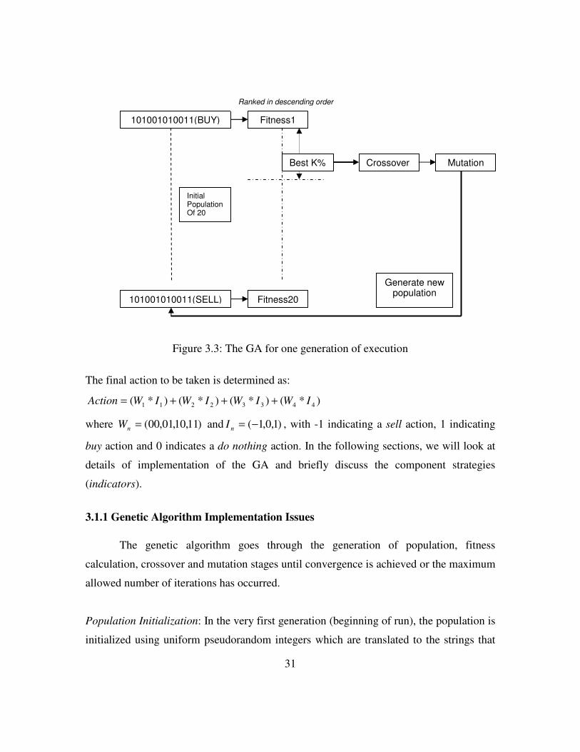
Figure 3.3: The GA for one generation of execution
The final action to be taken is determined as:
)*()*()*()*( 44332211 IWIWIWIWAction +++=
where )11,10,01,00(=nW and )1,0,1(−=nI , with -1 indicating a sell action, 1 indicating
buy action and 0 indicates a do nothing action. In the following sections, we will look at
details of implementation of the GA and briefly discuss the component strategies
(indicators).
3.1.1 Genetic Algorithm Implementation Issues
The genetic algorithm goes through the generation of population, fitness
calculation, crossover and mutation stages until convergence is achieved or the maximum
allowed number of iterations has occurred.
Population Initialization: In the very first generation (beginning of run), the population is
initialized using uniform pseudorandom integers which are translated to the strings that
101001010011(BUY)
101001010011(SELL)
Fitness1
Fitness20
Best K% Crossover Mutation
Initial Population Of 20
Generate new population
Ranked in descending order

32
constitute the initial population. We use a population of ten strings for each of the buy
and sell rules as the population for each generation. As can be seen in figure above, we
have 20 strings that populate every generation. Many factors go into choosing the size of
the population in a GA. Sufficient exploration of the search space necessitates a
reasonable size for the population. However, here, a mitigating factor was computation
time. Our training method included running the population over entire training periods
(15 days per training set), and a generation involved running 20 individuals
simultaneously on PXS over this entire period. This process took many hours (with 15
training days). For this reason, we found it necessary to keep the number of members in
the population down to a manageable number. However, we did introduce a few steps
like elitism (the selection of only the top ranking strings in terms of fitness) to encourage
convergence. Each subsequent generation is populated as a result of crossover and
mutation operations.
Fitness Calculation: The Sharpe and Sortino ratios (section 2.4) are used as the fitness
function to evaluate the performance of each member of a population in every generation.
The fitness was calculated as the Sharpe or Sortino ratio of the string over a period of
time (15 days if training sets in Appendix 2 are used). The training set of trading days
remained the same for each subsequent generation. Hence, the goal of the evolution
process is to maximize the fitness functions (and find the combination of weights that
does this) for a given set of training days. However, it is possible to find the right set of
weights to maximize the fitness over any given set of trading days (given sufficient time
and exploration), and we must keep in mind that the ultimate aim is to find the right
weights that will maximize profit over out-of-sample data (test data different from
training data). The strings of weights, after evaluation, are ranked in decreasing order of
fitness.
Crossover: Crossover is the process of cutting strategy string pairs at appropriate points
and exchanging tails between heads to make a new pair. Only the best k% of strategies is

33
used for crossover, and bit strings are crossed over tail to head. The probability of being
selected for crossover is higher for strategies with higher fitness.
The selection of a string ranked i is calculated by the formula:
pi =
��
��
�
���
��
� ≥−
�otherwise
Nkii
iNkNk
;0
.;.
.
1
where k is the percentage of population to be considered. N is the population size and i is
the rank of the string in the population. Based on this probability, pairs of strings are
independently selected (with replacement) from the population and crossed over [in a
manner as described in 21]. Once a pair has been selected, a cut point for both strings is
uniformly pseudo-randomly selected, so that both strings are cut into two pieces with the
‘head’ and ‘tail’ parts of both strings being the same length. Then these tails are crossed
over. The resulting strings are next analyzed to check uniqueness relative to the current
population by comparing each string bit by bit.
Mutation: Mutation is the process of randomly changing appropriate bits in a strategy
string and is executed in a bitwise manner. We maintain an elitist model since the top 2
strings (from each of the buy and sell sides) are spared mutation. This is done in order to
preserve strings with high fitness since in this kind of optimization we are searching for
maxima locally as well as globally, i.e. we attempt to generate an array of good solutions
rather than just the best. The generation of such a set of solutions rather than a single
good solution is done in an attempt to maintain a set of good solutions to search from
(and increase exploration). After each attempted mutation, the string is checked bit by bit
with the other solutions for uniqueness. In the event that duplicate strings are found, only
one of them is retained, and we dip into the remaining (unique) solutions and select the
one with the highest of the remaining fitness functions. Also, a brute force
implementation ensured that each generation had at least two sell and two buy rules
34
generated, to ensure that there was never a case when all rules were of sell or buy type
exclusively.
We use a relatively high mutation rate, to compensate for the small population
size, and to ensure more exploration of the search space. If the population of strings
contains B bits, numbered 1 to B, then we would wish to mutate M = 0.1B of them. In this
case, M uniform pseudo-random integers are generated between 1 and B without
replacement. The M integers are ordered by magnitude and for each the correspondingly
numbered bit is mutated (0 goes to 1, 1 goes to 0). After each string has been passed by
the mutation process, a bit-by-bit check is performed to test for uniqueness, and duplicate
strings are eliminated in favor of unique ones. Elitism also ensures that an arbitrary
stopping of the algorithm after a few generations produces a good result.
A lower bound on number of generations is used so even if it converges to a
maximum before that, it goes on until a set number of generations are done. Also, an
upper limit of generations was used to ensure that it doesn’t go on to the point where it
takes too much time (as we stressed earlier, the process already takes over a whole day of
runtime). Convergence is said to occur when mean fitness of a user defined percentage of
the most fit strategies and maximum fitness both change by no more than 1% between the
previous and current generation.
Figure 3.4(a) shows the convergence of the fitness over generations, for a training
run (with training set T1), and the respective weight values allotted in each generation. In
our thesis, we used a minimum number of generations as 8 (to ensure that local minima
are avoided) and a maximum number of 10 generations. This proved to be a very small
range, and owing to the fact that the GA almost always converged in 8 generations (in the
case of our tests), we might as well have done away with the range and stuck to a fixed
number of (eight) generations. Figure 3.4(b) shows the corresponding weights at each
generation for the one test run that we documented. It may be argued that the
convergence seems to have occurred in a fairly low number of generations only because
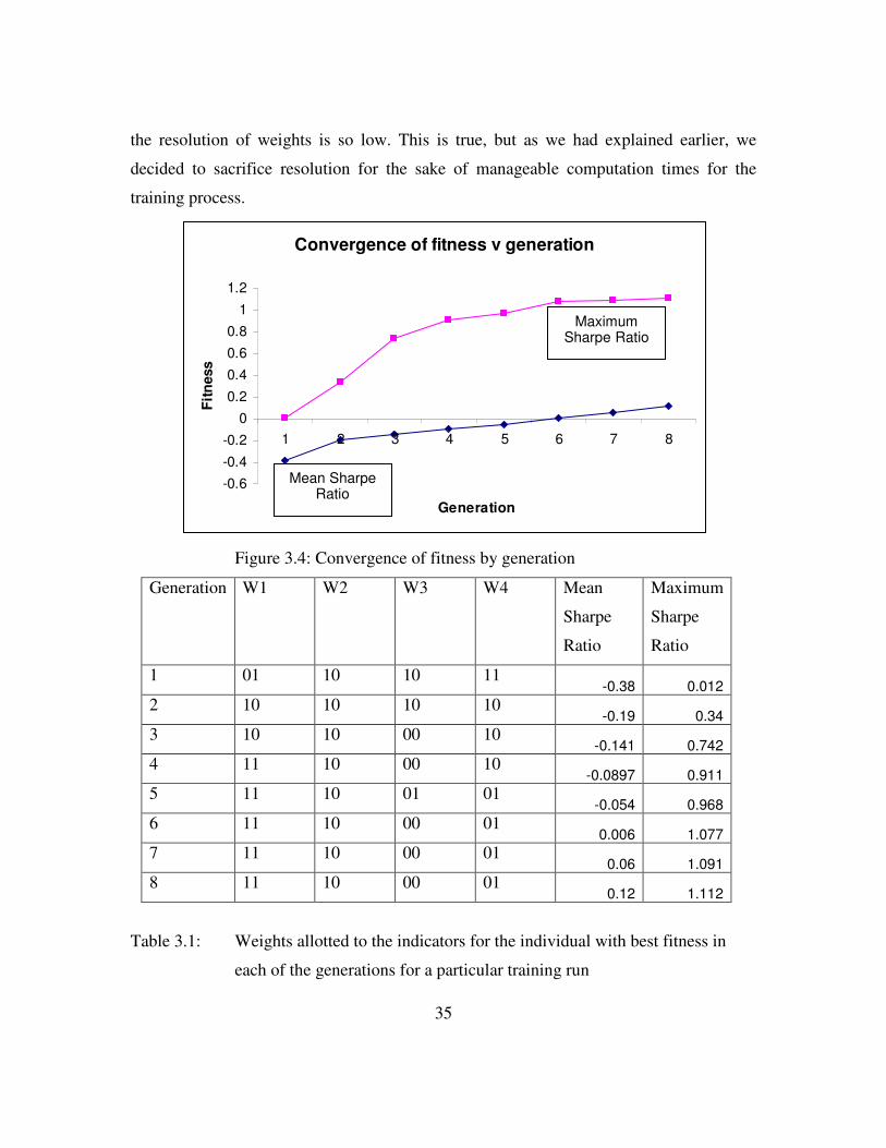
35
the resolution of weights is so low. This is true, but as we had explained earlier, we
decided to sacrifice resolution for the sake of manageable computation times for the
training process.
Convergence of fitness v generation
-0.6-0.4-0.2
00.20.40.60.8
11.2
1 2 3 4 5 6 7 8
Generation
Fitn
ess
Figure 3.4: Convergence of fitness by generation
Generation W1 W2 W3 W4 Mean
Sharpe
Ratio
Maximum
Sharpe
Ratio
1 01 10 10 11 -0.38 0.012
2 10 10 10 10 -0.19 0.34
3 10 10 00 10 -0.141 0.742
4 11 10 00 10 -0.0897 0.911
5 11 10 01 01 -0.054 0.968
6 11 10 00 01 0.006 1.077
7 11 10 00 01 0.06 1.091
8 11 10 00 01 0.12 1.112
Table 3.1: Weights allotted to the indicators for the individual with best fitness in
each of the generations for a particular training run
Maximum Sharpe Ratio
Mean Sharpe Ratio
36
3.1.2 Component Strategies or Indicators
So far, we have discussed how indicators are combined to produce a weighted
suggestion, and how this is used to arrive at a suitable trading action. We now look at the
component strategies that are used as indicators in the formulation discussed in earlier
sections. Although the strategies below are complete and give, as output, desired trading
action as well as the price and volume of the trading order to be placed, we implement
them as indicators alone. Thus, we only utilize the trading order suggestion from the
component technical trading strategies, and combine them using our weighted majority
algorithm to obtain trading volume.
At this point, we aim to clarify some implementation details, helping simplify
possible reconstruction of the experiments. Previously, we had assumed that once the
action was determined, it would be performed instantaneously. However, this is not
always the case. When a buy or sell order is placed, it is not necessary it will be filled. In
the event, a decision on the action to be performed was determined using the last price.
However, the actual execution involved looking at the order books and the existing
entries, and placing an order that is incrementally better than the best offer. The orders
placed were $0.0001 worse than the existing value. This value is small enough not to
make a substantial difference in price, yet helping the agent avoid much of the penalty for
removing liquidity in the order books by placing itself just behind the top order. In
pseudo code, this would be reflected as:
SellPrice = price of top sell order + 0.0001
BuyPrice = price of top buy order – 0.0001
We decided not to optimize the individual parameters (as suggested in section 3.1.1) in an
effort to avoid over-fitting the agent to the training data. So, the parameter choices, if
any, were determined empirically, over 15 sample days in the training set of days. In each
of our component strategies, we defined the order price to be the same and as described
above. We used a constant volume factor of 25 throughout the thesis. This volume factor
is the constant number of shares to be multiplied to the strength of the composite
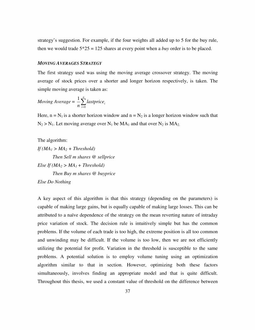
37
strategy’s suggestion. For example, if the four weights all added up to 5 for the buy rule,
then we would trade 5*25 = 125 shares at every point when a buy order is to be placed.
MOVING AVERAGES STRATEGY
The first strategy used was using the moving average crossover strategy. The moving
average of stock prices over a shorter and longer horizon respectively, is taken. The
simple moving average is taken as:
Moving Average = �=
n
iilastprice
n 0
1
Here, n = N1 is a shorter horizon window and n = N2 is a longer horizon window such that
N2 > N1. Let moving average over N1 be MA1 and that over N2 is MA2.
The algorithm:
If (MA1 > MA2 + Threshold)
Then Sell m shares @ sellprice
Else If (MA2 > MA1 + Threshold)
Then Buy m shares @ buyprice
Else Do Nothing
A key aspect of this algorithm is that this strategy (depending on the parameters) is
capable of making large gains, but is equally capable of making large losses. This can be
attributed to a naïve dependence of the strategy on the mean reverting nature of intraday
price variation of stock. The decision rule is intuitively simple but has the common
problems. If the volume of each trade is too high, the extreme position is all too common
and unwinding may be difficult. If the volume is too low, then we are not efficiently
utilizing the potential for profit. Variation in the threshold is susceptible to the same
problems. A potential solution is to employ volume tuning using an optimization
algorithm similar to that in section. However, optimizing both these factors
simultaneously, involves finding an appropriate model and that is quite difficult.
Throughout this thesis, we used a constant value of threshold on the difference between

38
two moving averages. The threshold was determined empirically. Setting it too low
would make the strategy too sensitive, and the true trend would probably not be captured.
Setting it too high would make it sluggish and unresponsive to anything but major
swings. We found that a value close to 0.01 proved to give good results. Also, window
sizes of 5 and 50 proved to yield good results.
VOLUME BASED STRATEGY
The strategy here remains the same as described in section 2.2.3. The basic strategy
involves obtaining the order book data for each update (in time, say t1) and getting the
corresponding volume of unmatched shares on the buy and sell sides of the book. The
difference of these volumes is the buy-sell difference. Then, this same difference is
obtained for the next time update (say time t2). The decision rule is stated as:
If (buy – sell)t2 > (buy – sell)t1 + Threshold
buyOrder(buyprice, ordervolume);
Else If (buy – sell)t1 > (buy – sell)t2 + Threshold
sellOrder(sellprice, ordervolume);
Else do nothing
In the volume based indicator strategy, a � factor of 0.1 proved to give us good
performance, where � was the multiplication factor in the volume threshold, Threshold =
�*(average of volumes in two order books).
SIMPLE PRICE BASED STRATEGY
This strategy is intuitively the simplest to understand. At any time during the simulation,
if the stock price goes up, it places a buy order; and if the stock price goes down, it places
a sell order. The motivation is that a price rise indicates likely further price rises. It is
written as:
If currentprice > lastprice
Buy @ buyprice (ordervolume)
Else if lastprice > currentprice
39
Sell @ sellprice (ordervolume)
Else Do Nothing
The strategy described here is the same as the one described in [5], where its performance
is compared to the ‘reverse’ strategy. The reason for choosing the direct strategy in the
face of results that prove otherwise is to allow for the GA to tune the weights and sign to
choose the (presumably superior) ‘reverse’ strategy if necessary. Essentially, the model
we propose includes a sign for the buy or sell order signaled by the component strategies,
allowing for use of the strategy in either form.
PRICE CHANNEL BREAKOUT STRATEGY
This strategy involves defining Bollinger bands [53], which enclose a price range within
the maximum and minimum price of the last few time steps. The trading range is defined
by the upper and lower bounds obtained by finding the maximum and minimum prices
over the last few time steps.
UpperPriceBandLimit = max(price over last n steps)
LowerPriceBandLimit = min(price over last n steps)
If CurrentPrice > UpperPriceBandLimit
Buy @ buyprice (ordervolume)
If CurrentPrice < LowerPriceBandLimit
Sell @ sellprice (ordervolume)
Else Do Nothing
When the price crosses the upper limit from below, it indicates a breakthrough and
signals a buy action. When the price crosses the lower limit from above, it signals a sell
action. This is a simple strategy to grasp intuitively. It is easy to imagine that this strategy
is useful more as support scheme to bolster a trading signal or to promote cautiousness in
trade. The above four indicators are abbreviated as MAS, VS, PS and PCBS respectively,
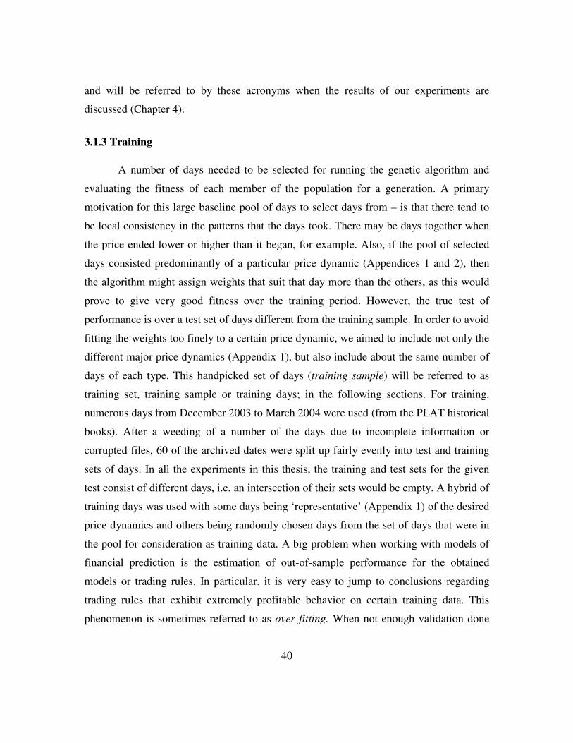
40
and will be referred to by these acronyms when the results of our experiments are
discussed (Chapter 4).
3.1.3 Training
A number of days needed to be selected for running the genetic algorithm and
evaluating the fitness of each member of the population for a generation. A primary
motivation for this large baseline pool of days to select days from – is that there tend to
be local consistency in the patterns that the days took. There may be days together when
the price ended lower or higher than it began, for example. Also, if the pool of selected
days consisted predominantly of a particular price dynamic (Appendices 1 and 2), then
the algorithm might assign weights that suit that day more than the others, as this would
prove to give very good fitness over the training period. However, the true test of
performance is over a test set of days different from the training sample. In order to avoid
fitting the weights too finely to a certain price dynamic, we aimed to include not only the
different major price dynamics (Appendix 1), but also include about the same number of
days of each type. This handpicked set of days (training sample) will be referred to as
training set, training sample or training days; in the following sections. For training,
numerous days from December 2003 to March 2004 were used (from the PLAT historical
books). After a weeding of a number of the days due to incomplete information or
corrupted files, 60 of the archived dates were split up fairly evenly into test and training
sets of days. In all the experiments in this thesis, the training and test sets for the given
test consist of different days, i.e. an intersection of their sets would be empty. A hybrid of
training days was used with some days being ‘representative’ (Appendix 1) of the desired
price dynamics and others being randomly chosen days from the set of days that were in
the pool for consideration as training data. A big problem when working with models of
financial prediction is the estimation of out-of-sample performance for the obtained
models or trading rules. In particular, it is very easy to jump to conclusions regarding
trading rules that exhibit extremely profitable behavior on certain training data. This
phenomenon is sometimes referred to as over fitting. When not enough validation done
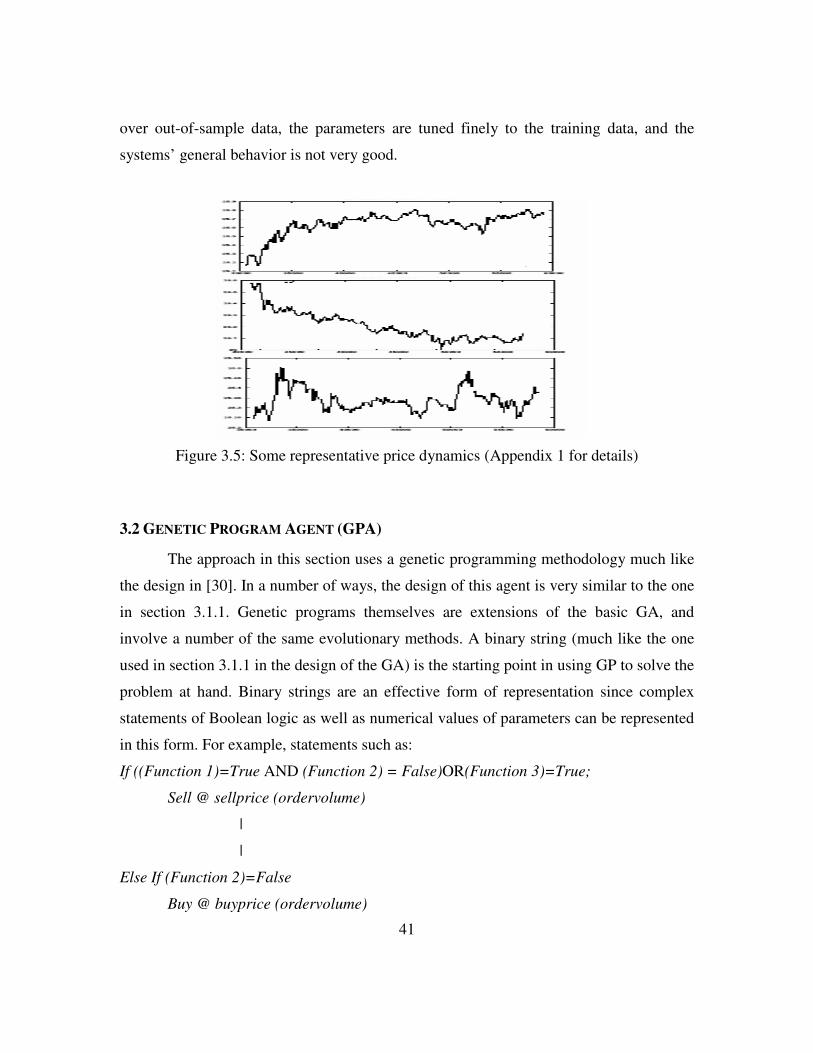
41
over out-of-sample data, the parameters are tuned finely to the training data, and the
systems’ general behavior is not very good.
Figure 3.5: Some representative price dynamics (Appendix 1 for details)
3.2 GENETIC PROGRAM AGENT (GPA)
The approach in this section uses a genetic programming methodology much like
the design in [30]. In a number of ways, the design of this agent is very similar to the one
in section 3.1.1. Genetic programs themselves are extensions of the basic GA, and
involve a number of the same evolutionary methods. A binary string (much like the one
used in section 3.1.1 in the design of the GA) is the starting point in using GP to solve the
problem at hand. Binary strings are an effective form of representation since complex
statements of Boolean logic as well as numerical values of parameters can be represented
in this form. For example, statements such as:
If ((Function 1)=True AND (Function 2) = False)OR(Function 3)=True;
Sell @ sellprice (ordervolume)
|
|
Else If (Function 2)=False
Buy @ buyprice (ordervolume)
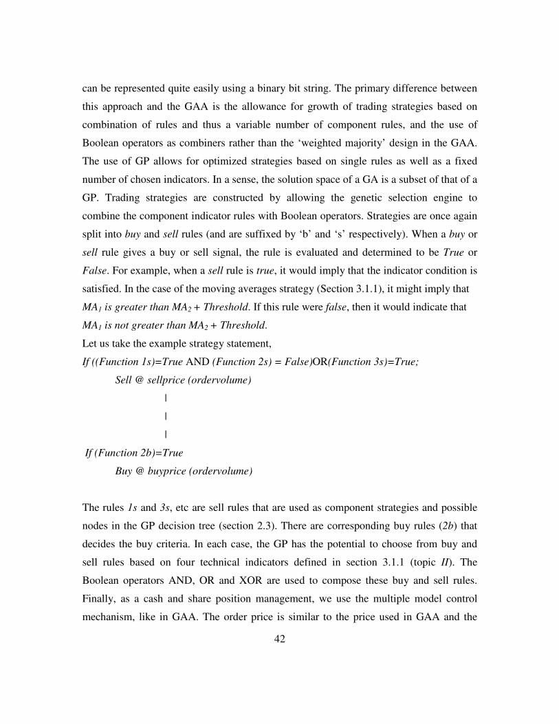
42
can be represented quite easily using a binary bit string. The primary difference between
this approach and the GAA is the allowance for growth of trading strategies based on
combination of rules and thus a variable number of component rules, and the use of
Boolean operators as combiners rather than the ‘weighted majority’ design in the GAA.
The use of GP allows for optimized strategies based on single rules as well as a fixed
number of chosen indicators. In a sense, the solution space of a GA is a subset of that of a
GP. Trading strategies are constructed by allowing the genetic selection engine to
combine the component indicator rules with Boolean operators. Strategies are once again
split into buy and sell rules (and are suffixed by ‘b’ and ‘s’ respectively). When a buy or
sell rule gives a buy or sell signal, the rule is evaluated and determined to be True or
False. For example, when a sell rule is true, it would imply that the indicator condition is
satisfied. In the case of the moving averages strategy (Section 3.1.1), it might imply that
MA1 is greater than MA2 + Threshold. If this rule were false, then it would indicate that
MA1 is not greater than MA2 + Threshold.
Let us take the example strategy statement,
If ((Function 1s)=True AND (Function 2s) = False)OR(Function 3s)=True;
Sell @ sellprice (ordervolume)
|
|
|
If (Function 2b)=True
Buy @ buyprice (ordervolume)
The rules 1s and 3s, etc are sell rules that are used as component strategies and possible
nodes in the GP decision tree (section 2.3). There are corresponding buy rules (2b) that
decides the buy criteria. In each case, the GP has the potential to choose from buy and
sell rules based on four technical indicators defined in section 3.1.1 (topic II). The
Boolean operators AND, OR and XOR are used to compose these buy and sell rules.
Finally, as a cash and share position management, we use the multiple model control
mechanism, like in GAA. The order price is similar to the price used in GAA and the

43
order volume in GPA was throughout this thesis is 125 – this value determined
empirically over 10 sample days. We abandoned attempts to include volume as a tuning
factor in this experiment, in order to simplify the design. The structure of the strategy as
well as the binary string has certain changes from the representation in GAA (Figure 3.6).
We have Boolean connectors and the use of rule in use bits that tell us whether a certain
rule is selected for use or not.
In Figure 3.7, we show how such a rule structure like the one in Figure 3.6
translates to a binary string. Each indicator has a particular bit that reflects that it is either
true or false by indicating 1 or 0, respectively. Also, each indicator pair has a Boolean
connector - AND, OR, XOR - represented by 00, 01 and 10, respectively. The last part of
the string indicates which indicators are to be ignored. This allows strategies containing
variable numbers of indicators to be represented without substantial change in design
from the GAA. Note that although the buy and sell rules are dependent on two and three
indicators, respectively, they are of the same length.
Rule 1 Rule 2
Rule 3 Rule 4
Rule1 Used?
Rule2 Used?
Rule3 Used?
Rule4 Used?
BUY
1 True
00 AND
1 True
01 OR
0 False
00 AND
1 True
1 Yes
0 No
1 Yes
0 No
Rule 1 Rule 2
Rule 3
Rule 4
Rule1 Used?
Rule2 Used?
Rule3 Used?
Rule4 Used?
SELL
1 True
00 AND
1 True
01 OR
0 False
10 XOR
1 True
1 Yes
1 Yes
1 Yes
0 No
Figure 3.6: Structure of buy and sell bit strings that populate the GP
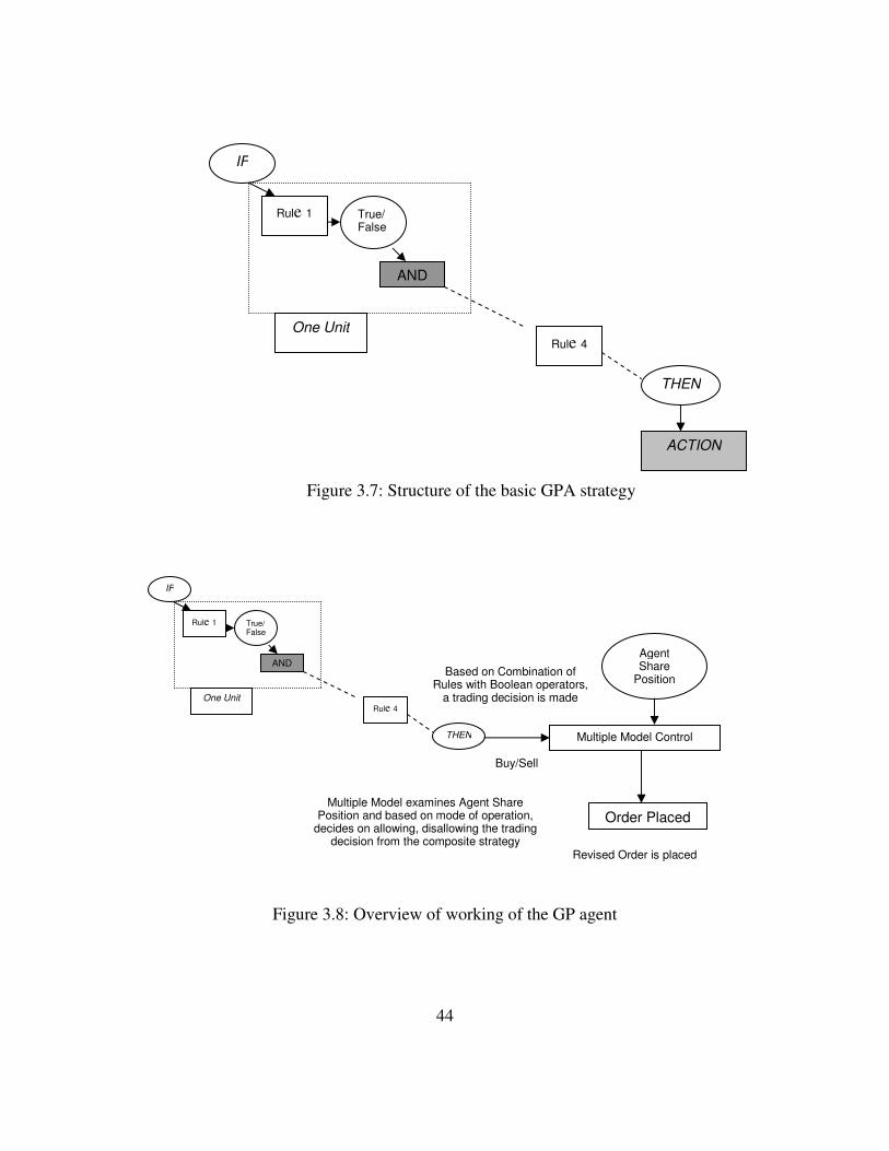
44
Figure 3.7: Structure of the basic GPA strategy
Figure 3.8: Overview of working of the GP agent
IF
Rule 1
Rule 4
True/ False
AND
THEN
One Unit
Based on Combination of Rules with Boolean operators,
a trading decision is made
Buy/Sell
Multiple Model Control
Agent Share
Position
Multiple Model examines Agent Share Position and based on mode of operation,
decides on allowing, disallowing the trading decision from the composite strategy
Order Placed
Revised Order is placed
IF
Rule 1
Rule 4
True/ False
AND
THEN
ACTION
One Unit

45
Each generation of evolving strategies in the GP follows the same steps (population
initialization, fitness calculation, crossover and mutation) as that of the GA (section
3.1.1) and the mechanics of these steps remain the same. Additionally, the training
process remains the same. Figure 3.8 shows how the change in this strategy is only in the
ME phase of the overall design, and the APE phase remains as it was in the GAA.

46
Chapter 4. Results and Analysis
This chapter is divided into two segments. The first segment contains
experiments, results and analysis with the primary focus being on developmental results,
and exploration of various schemes of optimization of our basic algorithm. The second
segment contains results and analysis of our composite strategy in competition scenarios
with other agents.
4.1 DESIGN OF EXPERIMENTS
Controlled experiments were performed to evaluate the evolutionary agents
individually. This selection process was followed by competitive experiments to validate
the performance of these evolutionary agents in joint simulations. The training days were
chosen to fairly represent different price dynamics (Figure 3.5). With a view to testing the
strategies in various environments, an effort was made to include different price
dynamics in the test set of days as well. The experimental test dates were chosen from
two distinct periods of time, one around December 2003 and the other around April 2004.
In addition to tests performed at various stages of development of the agents (in order to
evaluate certain hypotheses that we made earlier), we performed controlled, structured
experiments in a competitive environment with other agents whose underlying strategies
differed from our evolutionary agents as well as between themselves.
Evolutionary algorithms involve a fitness function (which is optimized) to arrive
at a solution or set of solutions that are ‘superior’ to the explored potential solutions in
the search space. However, a change in the fitness function could cause a change in the
‘fitness’ of the solution, and it may no longer be superior. Earlier, we looked at the
Sharpe and Modified Sortino ratios as validation criteria. We hypothesized that using
these measures as fitness functions in comparison tests could shed some light on the issue
and provide interesting results. A matrix of tests (Table 4.1) was performed in an effort to
perform this study.
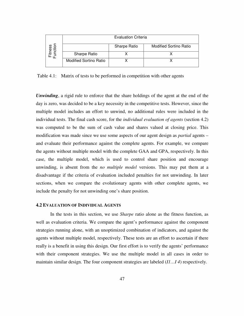
47
Table 4.1: Matrix of tests to be performed in competition with other agents
Unwinding, a rigid rule to enforce that the share holdings of the agent at the end of the
day is zero, was decided to be a key necessity in the competitive tests. However, since the
multiple model includes an effort to unwind, no additional rules were included in the
individual tests. The final cash score, for the individual evaluation of agents (section 4.2)
was computed to be the sum of cash value and shares valued at closing price. This
modification was made since we use some aspects of our agent design as partial agents –
and evaluate their performance against the complete agents. For example, we compare
the agents without multiple model with the complete GAA and GPA, respectively. In this
case, the multiple model, which is used to control share position and encourage
unwinding, is absent from the no multiple model versions. This may put them at a
disadvantage if the criteria of evaluation included penalties for not unwinding. In later
sections, when we compare the evolutionary agents with other complete agents, we
include the penalty for not unwinding one’s share position.
4.2 EVALUATION OF INDIVIDUAL AGENTS
In the tests in this section, we use Sharpe ratio alone as the fitness function, as
well as evaluation criteria. We compare the agent’s performance against the component
strategies running alone, with an unoptimized combination of indicators, and against the
agents without multiple model, respectively. These tests are an effort to ascertain if there
really is a benefit in using this design. Our first effort is to verify the agents’ performance
with their component strategies. We use the multiple model in all cases in order to
maintain similar design. The four component strategies are labeled (I1…I 4) respectively.
Evaluation Criteria
Sharpe Ratio Modified Sortino Ratio
Sharpe Ratio X X Fitn
ess
Func
tion
Modified Sortino Ratio X X
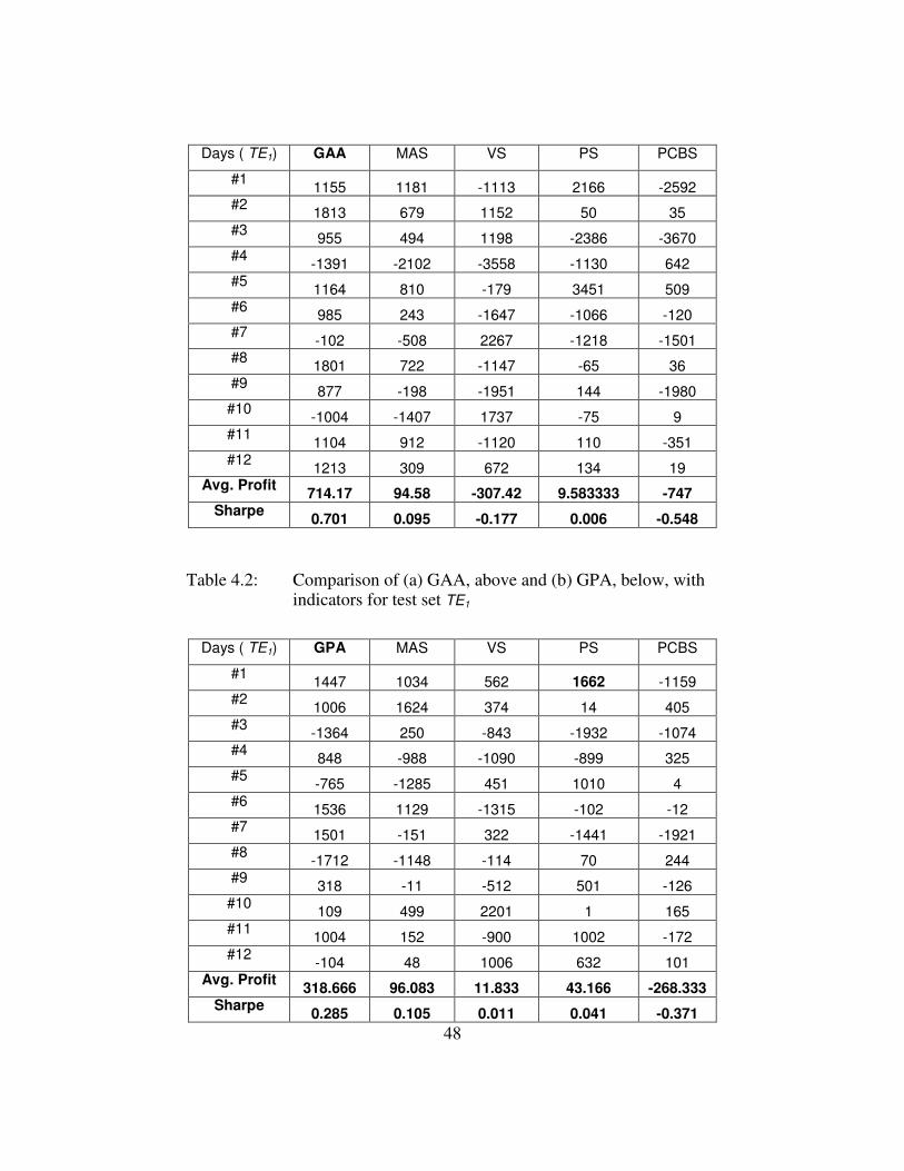
48
Table 4.2: Comparison of (a) GAA, above and (b) GPA, below, with indicators for test set TE1
Days ( TE1) GAA MAS VS PS PCBS
#1 1155 1181 -1113 2166 -2592 #2 1813 679 1152 50 35 #3 955 494 1198 -2386 -3670 #4 -1391 -2102 -3558 -1130 642 #5 1164 810 -179 3451 509 #6 985 243 -1647 -1066 -120 #7 -102 -508 2267 -1218 -1501 #8 1801 722 -1147 -65 36 #9 877 -198 -1951 144 -1980 #10 -1004 -1407 1737 -75 9 #11 1104 912 -1120 110 -351 #12 1213 309 672 134 19
Avg. Profit 714.17 94.58 -307.42 9.583333 -747 Sharpe 0.701 0.095 -0.177 0.006 -0.548
Days ( TE1) GPA MAS VS PS PCBS
#1 1447 1034 562 1662 -1159 #2 1006 1624 374 14 405 #3 -1364 250 -843 -1932 -1074 #4 848 -988 -1090 -899 325 #5 -765 -1285 451 1010 4 #6 1536 1129 -1315 -102 -12 #7 1501 -151 322 -1441 -1921 #8 -1712 -1148 -114 70 244 #9 318 -11 -512 501 -126 #10 109 499 2201 1 165 #11 1004 152 -900 1002 -172 #12 -104 48 1006 632 101
Avg. Profit 318.666 96.083 11.833 43.166 -268.333 Sharpe 0.285 0.105 0.011 0.041 -0.371
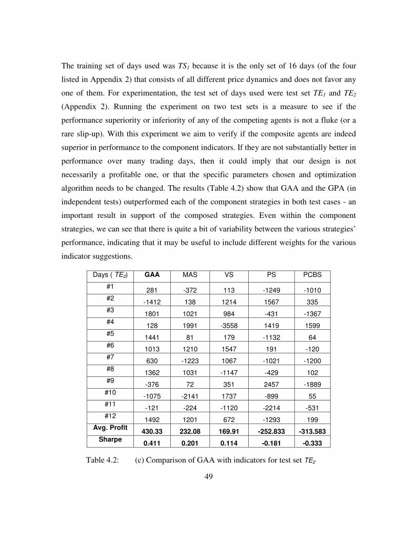
49
The training set of days used was TS1 because it is the only set of 16 days (of the four
listed in Appendix 2) that consists of all different price dynamics and does not favor any
one of them. For experimentation, the test set of days used were test set TE1 and TE2
(Appendix 2). Running the experiment on two test sets is a measure to see if the
performance superiority or inferiority of any of the competing agents is not a fluke (or a
rare slip-up). With this experiment we aim to verify if the composite agents are indeed
superior in performance to the component indicators. If they are not substantially better in
performance over many trading days, then it could imply that our design is not
necessarily a profitable one, or that the specific parameters chosen and optimization
algorithm needs to be changed. The results (Table 4.2) show that GAA and the GPA (in
independent tests) outperformed each of the component strategies in both test cases - an
important result in support of the composed strategies. Even within the component
strategies, we can see that there is quite a bit of variability between the various strategies’
performance, indicating that it may be useful to include different weights for the various
indicator suggestions.
Table 4.2: (c) Comparison of GAA with indicators for test set TE2
Days ( TE2) GAA MAS VS PS PCBS
#1 281 -372 113 -1249 -1010 #2 -1412 138 1214 1567 335 #3 1801 1021 984 -431 -1367 #4 128 1991 -3558 1419 1599 #5 1441 81 179 -1132 64 #6 1013 1210 1547 191 -120 #7 630 -1223 1067 -1021 -1200 #8 1362 1031 -1147 -429 102 #9 -376 72 351 2457 -1889 #10 -1075 -2141 1737 -899 55 #11 -121 -224 -1120 -2214 -531 #12 1492 1201 672 -1293 199
Avg. Profit 430.33 232.08 169.91 -252.833 -313.583 Sharpe 0.411 0.201 0.114 -0.181 -0.333
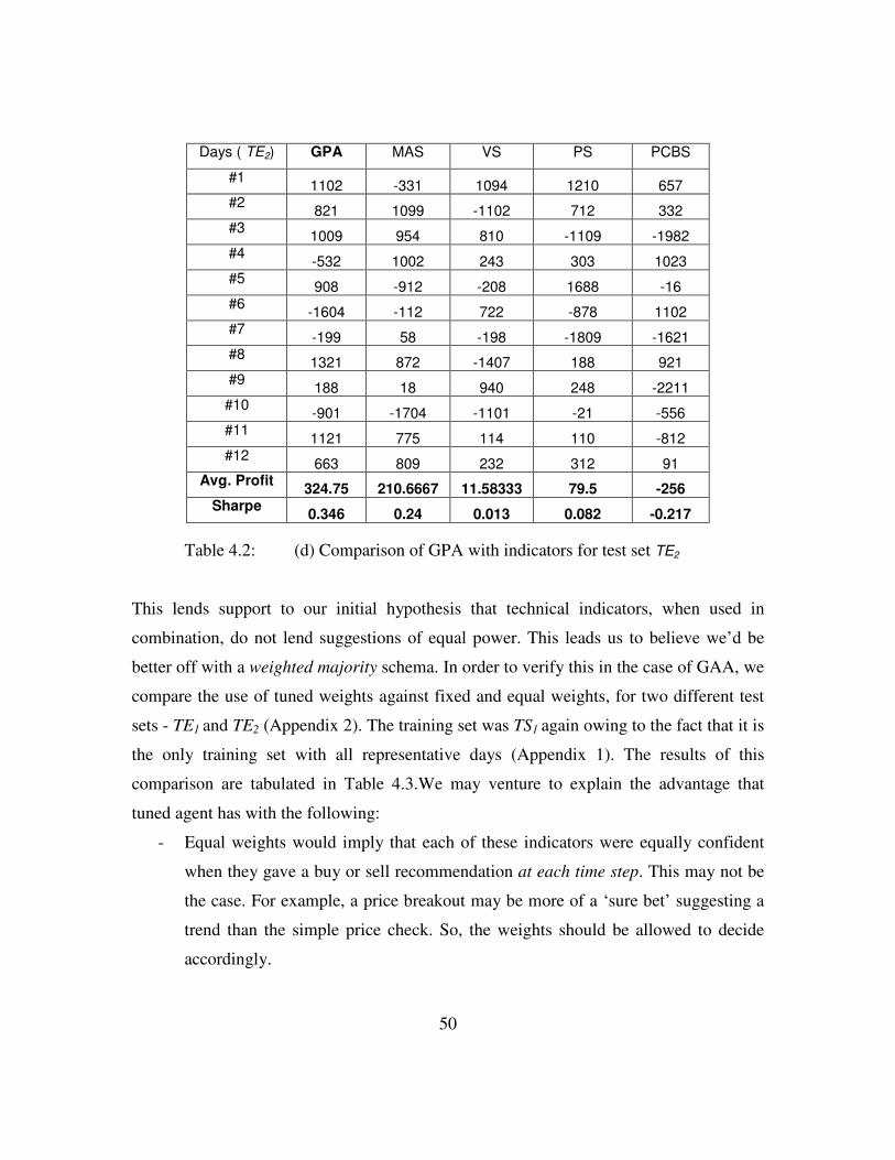
50
Table 4.2: (d) Comparison of GPA with indicators for test set TE2
This lends support to our initial hypothesis that technical indicators, when used in
combination, do not lend suggestions of equal power. This leads us to believe we’d be
better off with a weighted majority schema. In order to verify this in the case of GAA, we
compare the use of tuned weights against fixed and equal weights, for two different test
sets - TE1 and TE2 (Appendix 2). The training set was TS1 again owing to the fact that it is
the only training set with all representative days (Appendix 1). The results of this
comparison are tabulated in Table 4.3.We may venture to explain the advantage that
tuned agent has with the following:
- Equal weights would imply that each of these indicators were equally confident
when they gave a buy or sell recommendation at each time step. This may not be
the case. For example, a price breakout may be more of a ‘sure bet’ suggesting a
trend than the simple price check. So, the weights should be allowed to decide
accordingly.
Days ( TE2) GPA MAS VS PS PCBS
#1 1102 -331 1094 1210 657 #2 821 1099 -1102 712 332 #3 1009 954 810 -1109 -1982 #4 -532 1002 243 303 1023 #5 908 -912 -208 1688 -16 #6 -1604 -112 722 -878 1102 #7 -199 58 -198 -1809 -1621 #8 1321 872 -1407 188 921 #9 188 18 940 248 -2211 #10 -901 -1704 -1101 -21 -556 #11 1121 775 114 110 -812 #12 663 809 232 312 91
Avg. Profit 324.75 210.6667 11.58333 79.5 -256 Sharpe 0.346 0.24 0.013 0.082 -0.217
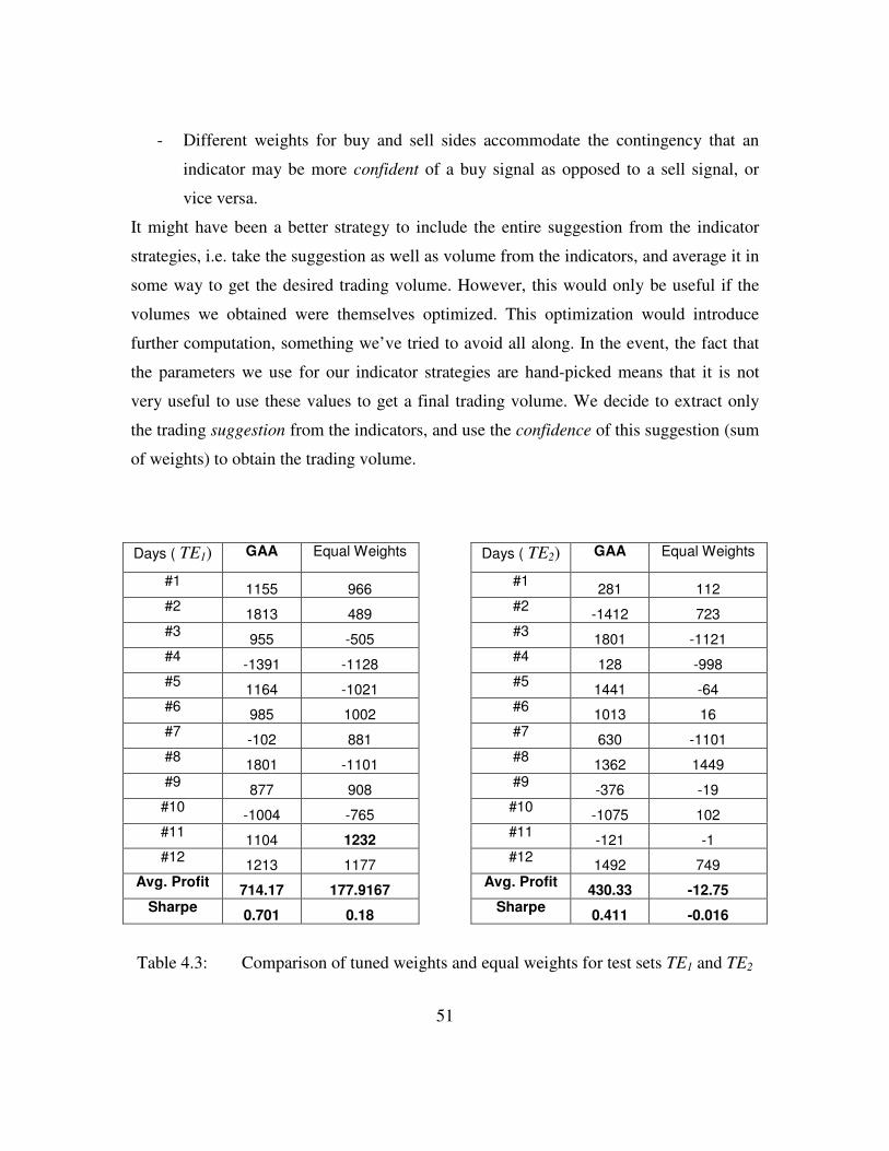
51
- Different weights for buy and sell sides accommodate the contingency that an
indicator may be more confident of a buy signal as opposed to a sell signal, or
vice versa.
It might have been a better strategy to include the entire suggestion from the indicator
strategies, i.e. take the suggestion as well as volume from the indicators, and average it in
some way to get the desired trading volume. However, this would only be useful if the
volumes we obtained were themselves optimized. This optimization would introduce
further computation, something we’ve tried to avoid all along. In the event, the fact that
the parameters we use for our indicator strategies are hand-picked means that it is not
very useful to use these values to get a final trading volume. We decide to extract only
the trading suggestion from the indicators, and use the confidence of this suggestion (sum
of weights) to obtain the trading volume.
Table 4.3: Comparison of tuned weights and equal weights for test sets TE1 and TE2
Days ( TE1) GAA Equal Weights
#1 1155 966 #2 1813 489 #3 955 -505 #4 -1391 -1128 #5 1164 -1021 #6 985 1002 #7 -102 881 #8 1801 -1101 #9 877 908 #10 -1004 -765 #11 1104 1232 #12 1213 1177
Avg. Profit 714.17 177.9167 Sharpe 0.701 0.18
Days ( TE2) GAA Equal Weights
#1 281 112 #2 -1412 723 #3 1801 -1121 #4 128 -998 #5 1441 -64 #6 1013 16 #7 630 -1101 #8 1362 1449 #9 -376 -19 #10 -1075 102 #11 -121 -1 #12 1492 749
Avg. Profit 430.33 -12.75 Sharpe 0.411 -0.016
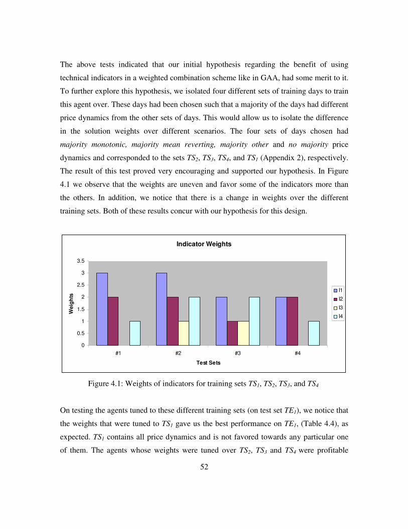
52
The above tests indicated that our initial hypothesis regarding the benefit of using
technical indicators in a weighted combination scheme like in GAA, had some merit to it.
To further explore this hypothesis, we isolated four different sets of training days to train
this agent over. These days had been chosen such that a majority of the days had different
price dynamics from the other sets of days. This would allow us to isolate the difference
in the solution weights over different scenarios. The four sets of days chosen had
majority monotonic, majority mean reverting, majority other and no majority price
dynamics and corresponded to the sets TS2, TS3, TS4, and TS1 (Appendix 2), respectively.
The result of this test proved very encouraging and supported our hypothesis. In Figure
4.1 we observe that the weights are uneven and favor some of the indicators more than
the others. In addition, we notice that there is a change in weights over the different
training sets. Both of these results concur with our hypothesis for this design.
Indicator Weights
0
0.5
1
1.5
2
2.5
3
3.5
#1 #2 #3 #4
Test Sets
Wei
ghts
I1
I2
I3
I4
Figure 4.1: Weights of indicators for training sets TS1, TS2, TS3, and TS4
On testing the agents tuned to these different training sets (on test set TE1), we notice that
the weights that were tuned to TS1 gave us the best performance on TE1, (Table 4.4), as
expected. TS1 contains all price dynamics and is not favored towards any particular one
of them. The agents whose weights were tuned over TS2, TS3 and TS4 were profitable
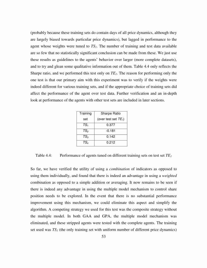
53
(probably because these training sets do contain days of all price dynamics, although they
are largely biased towards particular price dynamics), but lagged in performance to the
agent whose weights were tuned to TS1. The number of training and test data available
are so few that no statistically significant conclusion can be made from these. We just use
these results as guidelines to the agents’ behavior over larger (more complete datasets),
and to try and glean some qualitative information out of them. Table 4.4 only reflects the
Sharpe ratio, and we performed this test only on TE1. The reason for performing only the
one test is that our primary aim with this experiment was to verify if the weights were
indeed different for various training sets, and if the appropriate choice of training sets did
affect the performance of the agent over test data. Further verification and an in-depth
look at performance of the agents with other test sets are included in later sections.
Training
set
Sharpe Ratio
(over test set TE1)
TS1 0.377
TS2 -0.181
TS3 0.142
TS4 0.212
Table 4.4: Performance of agents tuned on different training sets on test set TE1
So far, we have verified the utility of using a combination of indicators as opposed to
using them individually, and found that there is indeed an advantage in using a weighted
combination as opposed to a simple addition or averaging. It now remains to be seen if
there is indeed any advantage in using the multiple model mechanism to control share
position needs to be explored. In the event that there is no substantial performance
improvement using this mechanism, we could eliminate this aspect and simplify the
algorithm. A competing strategy we used for this test was the composite strategy without
the multiple model. In both GAA and GPA, the multiple model mechanism was
eliminated, and these stripped agents were tested with the complete agents. The training
set used was TS1 (the only training set with uniform number of different price dynamics)
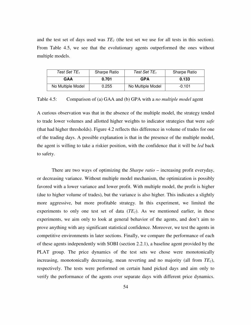
54
and the test set of days used was TE1 (the test set we use for all tests in this section).
From Table 4.5, we see that the evolutionary agents outperformed the ones without
multiple models.
Test Set TE1 Sharpe Ratio Test Set TE1 Sharpe Ratio
GAA 0.701 GPA 0.133
No Multiple Model 0.255 No Multiple Model -0.101
Table 4.5: Comparison of (a) GAA and (b) GPA with a no multiple model agent
A curious observation was that in the absence of the multiple model, the strategy tended
to trade lower volumes and allotted higher weights to indicator strategies that were safe
(that had higher thresholds). Figure 4.2 reflects this difference in volume of trades for one
of the trading days. A possible explanation is that in the presence of the multiple model,
the agent is willing to take a riskier position, with the confidence that it will be led back
to safety.
There are two ways of optimizing the Sharpe ratio – increasing profit everyday,
or decreasing variance. Without multiple model mechanism, the optimization is possibly
favored with a lower variance and lower profit. With multiple model, the profit is higher
(due to higher volume of trades), but the variance is also higher. This indicates a slightly
more aggressive, but more profitable strategy. In this experiment, we limited the
experiments to only one test set of data (TE1). As we mentioned earlier, in these
experiments, we aim only to look at general behavior of the agents, and don’t aim to
prove anything with any significant statistical confidence. Moreover, we test the agents in
competitive environments in later sections. Finally, we compare the performance of each
of these agents independently with SOBI (section 2.2.1), a baseline agent provided by the
PLAT group. The price dynamics of the test sets we chose were monotonically
increasing, monotonically decreasing, mean reverting and no majority (all from TE1),
respectively. The tests were performed on certain hand picked days and aim only to
verify the performance of the agents over separate days with different price dynamics.
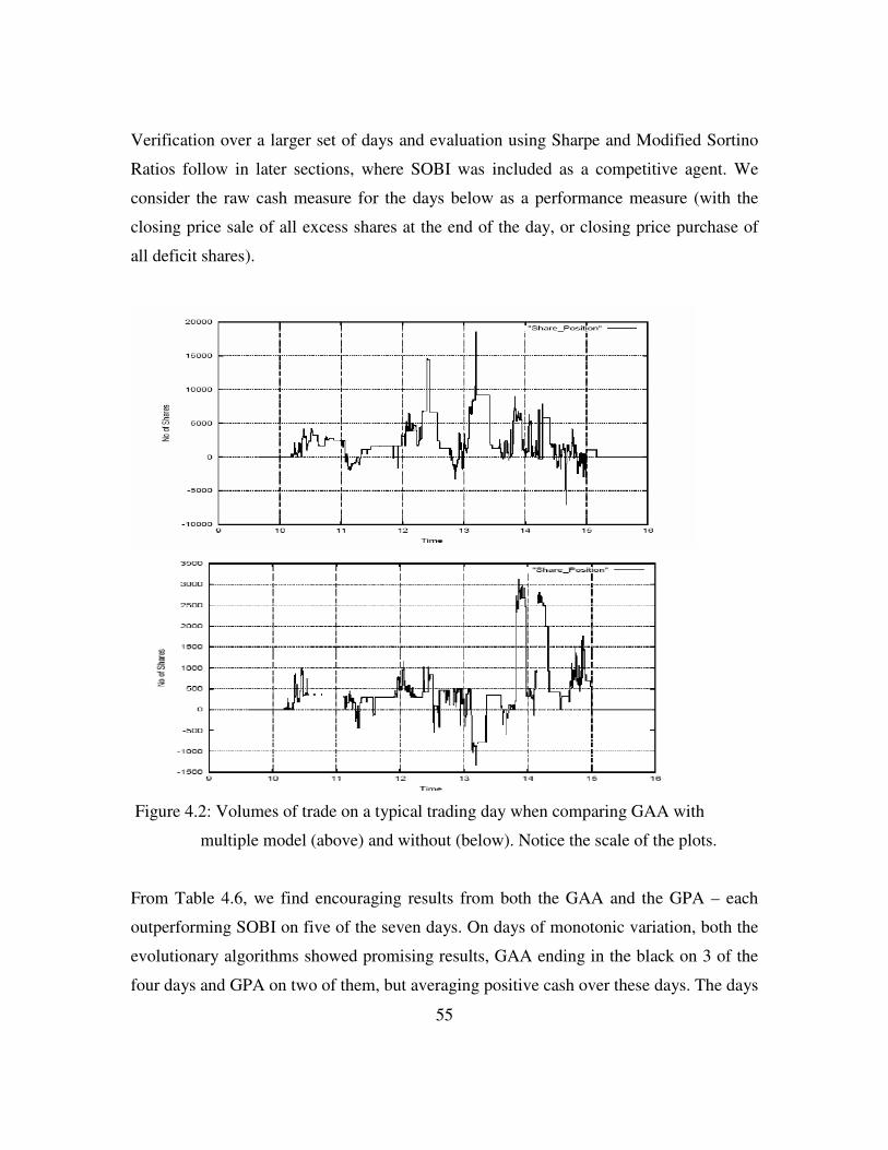
55
Verification over a larger set of days and evaluation using Sharpe and Modified Sortino
Ratios follow in later sections, where SOBI was included as a competitive agent. We
consider the raw cash measure for the days below as a performance measure (with the
closing price sale of all excess shares at the end of the day, or closing price purchase of
all deficit shares).
Figure 4.2: Volumes of trade on a typical trading day when comparing GAA with
multiple model (above) and without (below). Notice the scale of the plots.
From Table 4.6, we find encouraging results from both the GAA and the GPA – each
outperforming SOBI on five of the seven days. On days of monotonic variation, both the
evolutionary algorithms showed promising results, GAA ending in the black on 3 of the
four days and GPA on two of them, but averaging positive cash over these days. The days
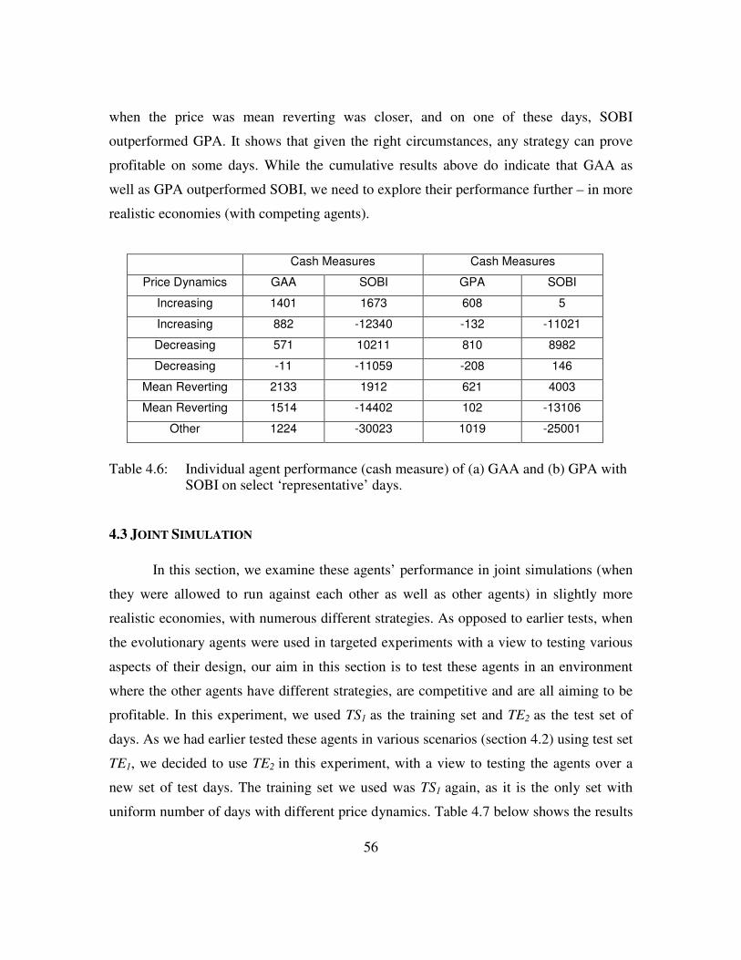
56
when the price was mean reverting was closer, and on one of these days, SOBI
outperformed GPA. It shows that given the right circumstances, any strategy can prove
profitable on some days. While the cumulative results above do indicate that GAA as
well as GPA outperformed SOBI, we need to explore their performance further – in more
realistic economies (with competing agents).
Cash Measures Cash Measures
Price Dynamics GAA SOBI GPA SOBI
Increasing 1401 1673 608 5
Increasing 882 -12340 -132 -11021
Decreasing 571 10211 810 8982
Decreasing -11 -11059 -208 146
Mean Reverting 2133 1912 621 4003
Mean Reverting 1514 -14402 102 -13106
Other 1224 -30023 1019 -25001
Table 4.6: Individual agent performance (cash measure) of (a) GAA and (b) GPA with SOBI on select ‘representative’ days.
4.3 JOINT SIMULATION
In this section, we examine these agents’ performance in joint simulations (when
they were allowed to run against each other as well as other agents) in slightly more
realistic economies, with numerous different strategies. As opposed to earlier tests, when
the evolutionary agents were used in targeted experiments with a view to testing various
aspects of their design, our aim in this section is to test these agents in an environment
where the other agents have different strategies, are competitive and are all aiming to be
profitable. In this experiment, we used TS1 as the training set and TE2 as the test set of
days. As we had earlier tested these agents in various scenarios (section 4.2) using test set
TE1, we decided to use TE2 in this experiment, with a view to testing the agents over a
new set of test days. The training set we used was TS1 again, as it is the only set with
uniform number of days with different price dynamics. Table 4.7 below shows the results
57
of the first joint simulation we performed. In addition to GAA and GPA, we use
competing agents SOBI, Market Maker (MM) and Volume-based agent (VBA). We
discussed these competing agents in Section 2.2. However, our aim in this section is only
to compare the performance of the GAA and GPA agents and evaluate the usefulness of
the Modified Sortino Ratio (MSR) as a fitness function in our design. We evaluate these
agents in a competitive test in later sections. Columns 1 and 2 of Table 4.7 display the
result of tests performed on GAA and GPA when they were tuned with Sharpe ratio as
the fitness function in training phase. Columns 3 and 4 of the table show the results of
similar tests performed on the evolutionary agents with Modified Sortino Ratio as the
fitness function. We also evaluate the agents below using the Sharpe and Modified
Sortino ratios, and additionally the raw profit (cash) score, as performance criteria; in
order to verify our hypothesis that the agents tuned to maximize profits and avoid only
negative volatility would do better than those which aimed to reduce all volatility. We
used the standard PLAT scoring policy and rules (discussed in Section 2.1.4), and enforce
unwinding penalties (in accordance with the rules imposed by the PLAT group in earlier
competitions).
At this point, as a means of evaluating the improvement in performance of agent,
we introduce a measure called the MSR to Sharpe ratio. This is the ratio of the values of
MSR and Sharpe ratios for a given column in our table. We see that GAA and GPA
(tuned with Sharpe ratio) showed values of 2.34 and 2.23 respectively, for this measure.
This value for GAA and GPA tuned with MSR was 5.12 and 2.49 respectively. We
observed that the agents tuned with MSR not only showed higher MSR values, but also
Sharpe ratios not too far below the SR-tuned agents. The difference between MSR and
Sharpe ratios was most stark in the case of GAA. This, coupled with the fact that the
Sharpe ratio was not too far off for GAA-MSR as compared to GAA-SR, is a good
indicator of the usefulness of the new fitness function in GAA. Also, from Figure 4.3 and
Table 4.7, we notice that the average profit as well as maximum profit was also higher for
GAA tuned with MSR. In the case of GPA, the MSR version did perform better than the
SR version in the MSR evaluation (and was very close in Sharpe ratio too), but the
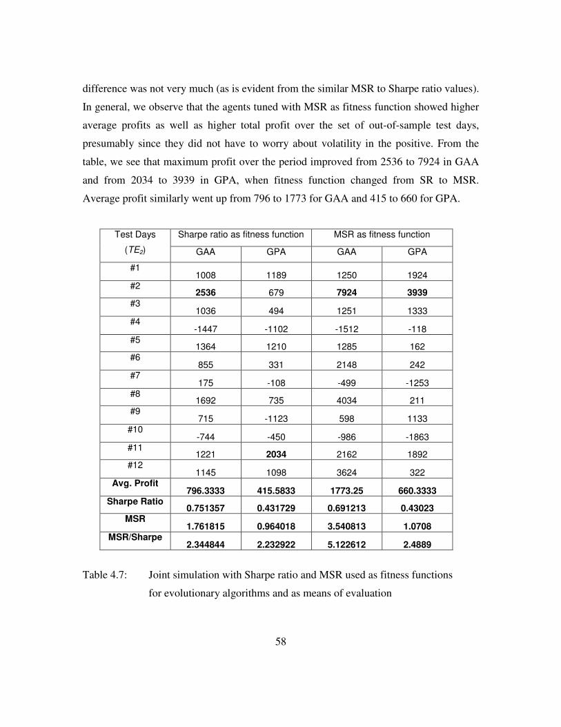
58
difference was not very much (as is evident from the similar MSR to Sharpe ratio values).
In general, we observe that the agents tuned with MSR as fitness function showed higher
average profits as well as higher total profit over the set of out-of-sample test days,
presumably since they did not have to worry about volatility in the positive. From the
table, we see that maximum profit over the period improved from 2536 to 7924 in GAA
and from 2034 to 3939 in GPA, when fitness function changed from SR to MSR.
Average profit similarly went up from 796 to 1773 for GAA and 415 to 660 for GPA.
Sharpe ratio as fitness function MSR as fitness function Test Days
(TE2) GAA GPA GAA GPA
#1 1008 1189 1250 1924
#2 2536 679 7924 3939
#3 1036 494 1251 1333
#4 -1447 -1102 -1512 -118
#5 1364 1210 1285 162
#6 855 331 2148 242
#7 175 -108 -499 -1253
#8 1692 735 4034 211
#9 715 -1123 598 1133
#10 -744 -450 -986 -1863
#11 1221 2034 2162 1892
#12 1145 1098 3624 322
Avg. Profit 796.3333 415.5833 1773.25 660.3333
Sharpe Ratio 0.751357 0.431729 0.691213 0.43023
MSR 1.761815 0.964018 3.540813 1.0708
MSR/Sharpe 2.344844 2.232922 5.122612 2.4889
Table 4.7: Joint simulation with Sharpe ratio and MSR used as fitness functions
for evolutionary algorithms and as means of evaluation
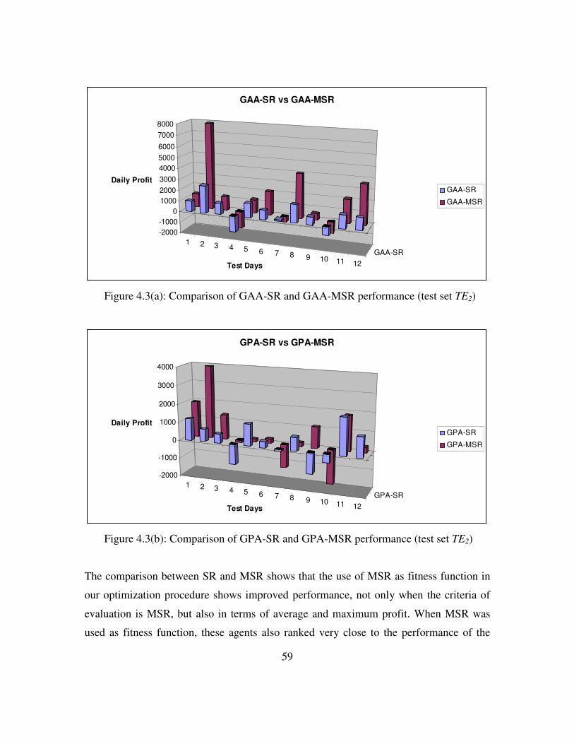
59
1 2 3 4 5 6 7 8 9 10 11 12GAA-SR
-2000-1000
010002000300040005000600070008000
Daily Profit
Test Days
GAA-SR vs GAA-MSR
GAA-SR
GAA-MSR
Figure 4.3(a): Comparison of GAA-SR and GAA-MSR performance (test set TE2)
1 2 3 4 5 6 7 8 9 10 11 12GPA-SR
-2000
-1000
0
1000
2000
3000
4000
Daily Profit
Test Days
GPA-SR vs GPA-MSR
GPA-SR
GPA-MSR
Figure 4.3(b): Comparison of GPA-SR and GPA-MSR performance (test set TE2)
The comparison between SR and MSR shows that the use of MSR as fitness function in
our optimization procedure shows improved performance, not only when the criteria of
evaluation is MSR, but also in terms of average and maximum profit. When MSR was
used as fitness function, these agents also ranked very close to the performance of the

60
SR-tuned agents, even when SR was used to evaluate these agents. Earlier, we had
hypothesized that the elimination of penalty for positive volatility would help improve
profitability, as we were penalizing agents for making large amounts of profits on a
trading day as much as we were penalizing them for losing large amounts on a day
(through the use of standard deviation). The results in this section validate our
hypothesis, and indicate that the use of better fitness functions, like MSR (which
penalizes only money losing behavior) may be a key factor in designing evolutionary
agents such as the ones in this thesis.
4.4 COMPETITIVE TESTS WITH OTHER AGENTS
In competitive tests, we use all four agents (GAA and GPA, each tuned with
Sharpe ratio and MSR) from the previous section, in addition to which we use SOBI,
MM and Multiple Model Agent (MuMo)[10a] – the last two were winners in two
previous competitions held in December 2003 and April 2004 (Appendix 3) respectively,
and were used to benchmark the performance of our evolutionary algorithms against
competitive agents. For the sake of readability, the GAA with Sharpe ratio as fitness
function was labeled GAA-SR and that with MSR as fitness function was labeled GAA-
MSR. The GPA counterparts were labeled GPA-SR and GPA-MSR respectively. The
training set for this run was TS1 again owing to the unbiased distribution of price
dynamics among the days in this set. To test the agents in a competitive test with
successful agents from past competitions, and to do so on days that were not used in
training or tests before, we use TE3 (Appendix 2) as the test set. In this test, we did not
use other agents such as the individual indicator strategies (section 3.1) since we had
already tested them over two datasets in previous tests (section 4.2). Also, we aimed to
limit the number of agents used in the test so computation as well as documentation
would be easier. Apart from the changes discussed above, the rules remained the same as
in the case of joint simulation (section 4.3). Table 4.8 below lays out the results of this
experiment.
The results of this experiment show that the performance of the evolutionary agents was
fairly competitive with the best agents from previous competitions (MM and MuMo) and
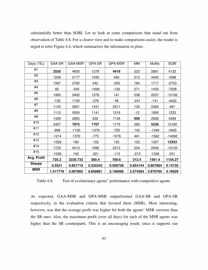
61
substantially better than SOBI. Let us look at some comparisons that stand out from
observation of Table 4.8. For a clearer view and to make comparisons easier, the reader is
urged to refer Figure 4.4, which summarizes the information in plots.
Table 4.8: Test of evolutionary agents’ performance with competitive agents
As expected, GAA-MSR and GPA-MSR outperformed GAA-SR and GPA-SR
respectively, in the evaluation criteria that favored them (MSR). Most interesting,
however, was that the average profit was higher for both the agents’ MSR versions than
the SR ones. Also, the maximum profit (over all days) for each of the MSR agents was
higher than the SR counterparts. This is an encouraging result, since it supports our
Days (TE3) GAA-SR GAA-MSR GPA-SR GPA-MSR MM MuMo SOBI
#1 2526 4655 1278 4416 223 2891 4133 #2 1249 2177 1045 492 312 3445 1698 #3 1567 2765 242 -253 184 1717 -2753 #4 82 -545 -1694 -130 271 1433 -7028 #5 1900 2402 1376 141 538 2037 -12182 #6 -132 1100 -376 49 -241 -141 -4422 #7 1145 2601 1441 2011 135 2465 481 #8 1112 5500 1141 1216 -12 1850 1233 #9 1429 2802 630 1134 656 2928 4399 #10 2457 7975 1707 1175 385 5229 12180 #11 -899 -1100 -1376 -755 142 -1349 -3405 #12 -1214 -1370 -775 -1076 461 -1562 -14092 #13 -1029 184 -102 125 122 1307 12333 #14 1723 4213 1090 2212 224 2509 -10120 #15 -1038 102 -221 -113 -213 -1338 231
Avg. Profit 725.2 2230.733 360.4 709.6 212.4 1561.4 1154.27 Sharpe 0.5521 0.851719 0.335342 0.509728 0.854144 0.807884 0.14735
MSR 1.517778 5.007865 0.658961 2.196996 2.574284 2.670785 0.18029
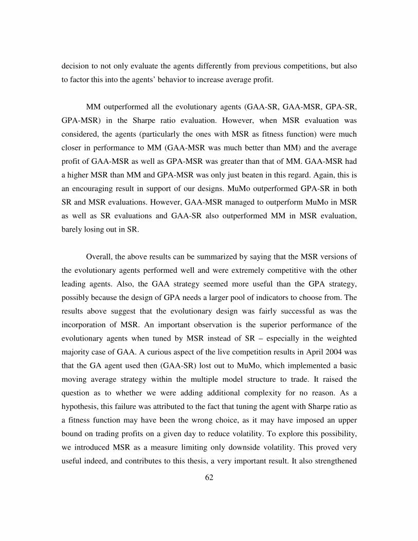
62
decision to not only evaluate the agents differently from previous competitions, but also
to factor this into the agents’ behavior to increase average profit.
MM outperformed all the evolutionary agents (GAA-SR, GAA-MSR, GPA-SR,
GPA-MSR) in the Sharpe ratio evaluation. However, when MSR evaluation was
considered, the agents (particularly the ones with MSR as fitness function) were much
closer in performance to MM (GAA-MSR was much better than MM) and the average
profit of GAA-MSR as well as GPA-MSR was greater than that of MM. GAA-MSR had
a higher MSR than MM and GPA-MSR was only just beaten in this regard. Again, this is
an encouraging result in support of our designs. MuMo outperformed GPA-SR in both
SR and MSR evaluations. However, GAA-MSR managed to outperform MuMo in MSR
as well as SR evaluations and GAA-SR also outperformed MM in MSR evaluation,
barely losing out in SR.
Overall, the above results can be summarized by saying that the MSR versions of
the evolutionary agents performed well and were extremely competitive with the other
leading agents. Also, the GAA strategy seemed more useful than the GPA strategy,
possibly because the design of GPA needs a larger pool of indicators to choose from. The
results above suggest that the evolutionary design was fairly successful as was the
incorporation of MSR. An important observation is the superior performance of the
evolutionary agents when tuned by MSR instead of SR – especially in the weighted
majority case of GAA. A curious aspect of the live competition results in April 2004 was
that the GA agent used then (GAA-SR) lost out to MuMo, which implemented a basic
moving average strategy within the multiple model structure to trade. It raised the
question as to whether we were adding additional complexity for no reason. As a
hypothesis, this failure was attributed to the fact that tuning the agent with Sharpe ratio as
a fitness function may have been the wrong choice, as it may have imposed an upper
bound on trading profits on a given day to reduce volatility. To explore this possibility,
we introduced MSR as a measure limiting only downside volatility. This proved very
useful indeed, and contributes to this thesis, a very important result. It also strengthened
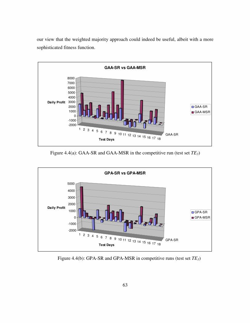
63
our view that the weighted majority approach could indeed be useful, albeit with a more
sophisticated fitness function.
1 2 3 4 5 6 7 8 9 10 11 12 13 14 15 16 17 18GAA-SR
-2000-1000
010002000300040005000600070008000
Daily Profit
Test Days
GAA-SR vs GAA-MSR
GAA-SR
GAA-MSR
Figure 4.4(a): GAA-SR and GAA-MSR in the competitive run (test set TE3)
1 2 3 4 5 6 7 8 9 10 11 12 13 14 15 16 17 18GPA-SR
-2000
-1000
0
1000
2000
3000
4000
5000
Daily Profit
Test Days
GPA-SR vs GPA-MSR
GPA-SR
GPA-MSR
Figure 4.4(b): GPA-SR and GPA-MSR in competitive runs (test set TE3)

64
1 2 3 4 5 6 7 8 9 10 11 12 13 14 15 16 17 18MM
-15000
-10000
-5000
0
5000
10000
15000
Daily Profit
Test Days
MM, MuMo and SOBI
MM
MuMo
SOBI
Figure 4.4(c): MM, MuMo and SOBI in competitive runs (test set TE3)
65
Chapter 5. Conclusions and Future Work
In this thesis, we have explored applications of evolutionary algorithms (GA and
GP) to technical trading rules in an effort to develop profitable agents for trade in the
PLAT domain, as well as to provide insight into the utility of such design to automated
trading scenarios. An important factor to consider is that this research was performed
purely as a study of certain agent schemes and as an exploration into the use of
evolutionary algorithms in the PLAT domain. Various limitations were imposed during
the course of this work, and although PXS is more realistic than most of the simulators
used in previous such studies, it is far from being realistic. The results in this thesis are
strictly within the confines of the test economy and no reasonable guarantees can be
made regarding its utility (as is) in actual trade markets. Our aim was to study the
implications of certain design aspects in a simulation and the study aims to be a launch
pad to more advanced and sophisticated agent designs of a similar nature.
Various studies have shown the benefits of technical trading as an effective day
trading strategy. However, their utility as effective strategies when used individually or in
combination but without the benefit of human ‘intuition’ has proven quite low. We have
found in this thesis that it is possible to profit from trading technical rules when the trade
entry signal is taken from combinations of indicators since this is the manner in which a
technical trader would use such indicators. The above work is just a sample of what can
be produced using such a system. Further adaptation techniques could include periodic
re-optimization with longer and shorter periods. As was previously stated, this first test of
our system aims to show that such a structure merits further work by analyzing results in
a general and unoptimized framework.
In this thesis, we proposed two frameworks for combining technical trading rules
in an effort to trade profitably in the PLAT domain. While the GPA design proved to be
only moderately successful in tests, it might have greater utility if parameter optimization
was done, especially the trading order volume. In this design, we used a fixed number
66
(arrived at empirically). Including volume in the bit string for a GPA-like design may be
a possible solution. We did not explore this idea further, but suggest it as a possible fix.
The GAA design proved much more successful and not only outperformed GPA and the
baseline SOBI agent, but also beat or proved very competitive when pitted with
successful agents from previous competitions in our battery of tests. We found that GAA
performs better than its component indicator strategies. To test if any combination of
technical rules would do, we compared our weighted majority algorithm with an agent
where the component indicators were combined with each of them weighted equally.
Superior performance of our weighted agents vindicated our decision to use evolutionary
algorithms to optimize weights for GAA. Further, the use of multiple model share
position control mechanism seemed to provide for unwinding while performing better
than the basic agents without the multiple model. In further tests of the agent against
competitive agents over different test sets of trading days, GAA proved to be profitable
and better or as good as the most successful of existing agents in the PLAT domain.
The evolutionary agents (particularly GAA) were fairly successful, but not quite
competitive with the successful PLAT agents until we used a new fitness function
(MSR), that penalized only loss making volatility and not all volatility (as Sharpe ratio
does). When the agents used MSR as fitness function, they proved to have improved
performance including greater profitability. This leads us to believe that there is useful
information in technical indicators that can be exploited, and further development and the
use of carefully chosen fitness functions might mean that such a design may prove to be
even more successful. This is consistent with the claims of technical analysis. The use of
multiple model mechanism also proved quite effective as a control element to the
strategy, allowing our agents to ‘boldly’ hold positions with the confidence of being
shepherded back to a desirable state by this mechanism. The qualitative nature of this
mechanism also appeals to intuition, and this was in keeping with our theme of using an
intuitive combination of technical rules. By implementing a simple set of weights,
various human trader-like behaviors could be replicated. These include deciding how

67
important a certain indicator is, and dropping certain indicators if they showed
consistently poor performance (by turning the weight down to zero).
What is evident is that more work has to be done in areas such as bit string
representation, fitness function choice and online optimization. Possible improvements
include finer resolution of weights using longer bit strings, the use of more indicators,
and development of more sophisticated fitness functions to include details finer than just
measures of profit and deviation over many days. Other feature additions could include a
method to run this optimization algorithm online (as a background process) and include
training days on the fly. This would make the agent more adaptive to immediate changes
and eliminate the need for time-intensive and periodic offline training.
This thesis is a small part of growing research in which computer-simulated
market interactions of autonomous agents are studied and an attempt is made not only to
develop a profitable trading strategy, but through these efforts, understand the working of
the market itself. The thesis provides us with a few solution concepts to certain aspects of
the automated trading problem, but has not been tested with any statistical significance
and the results we have obtained are by no means an indication that it is ready to be
deployed in the real world. It does point us (and walk us part of the way) towards
possible solution ideas that may be incorporated with further work to increase
profitability among automated trading agents. In a lot of ways, this thesis confirms the
difficulty of automated stock trading and suggests that further exploration of heuristic
solutions that may aid profitable trading is merited.
68
Appendix 1
MSFT Trading Prices and Price Dynamics
In this section, we aim to explain what we mean by price dynamics and briefly look at
some of the prominent price dynamics that we isolate for studying agent behavior under
different conditions.
High-frequency data, as we use the term, are observations taken many times a day. Price
dynamics, in the context we use it in, refers to a broad characterization of this intraday
data over the entire trading day. In other words, we try and fit (an approximate fit)
patterns to the daily data. Of course, we do not use any modeling or curve-fitting
technique, but use very broad, intuitive labeling.
Details such as opening price, closing price, high and low prices of the day – for a few
sample days of each type of price dynamic we use, are listed in tables below; followed by
a plot of the day’s price variation. All data is of Microsoft Stock (Symbol: MSFT).
For monotonically increasing data, we choose days that not only ended higher than
opening price, but spent most of the day increasing in price.
Days Opening High Low Closing
12/26/03 27.05 27.25 27.00 27.21
12/29/03 27.21 27.53 27.16 27.46
01/06/04 28.19 28.28 28.07 28.24
69
12/26/03 12/29/03 01/06/04
Similarly, for monotonically decreasing data, we choose days that end lower than the
opening price, and spend most of the day decreasing in price.
Days Opening High Low Closing
01/08/04 28.39 28.48 28.00 28.16
01/13/04 27.55 27.62 27.24 27.43
04/28/04 27.01 27.05 26.47 26.56
01/08/04 01/13/04 04/28/04
Mean reverting days imply days that ended within a small margin of the starting price
(we use 05.0± of a dollar as the margin). Additionally, these days spend substantial
amount of time on either side of the mean daily price.

70
Days Opening High Low Closing
04/26/04 27.45 27.55 27.10 27.44
05/05/04 26.32 26.60 26.25 26.30
05/06/04 26.16 26.34 26.03 26.12
04/28/04 05/05/04 05/06/04
All other patterns (or sub-patterns within the day) were more generally clubbed together
and labeled as other.
A more keen method of classifying the days might help increase the accuracy of our
experiments. However, owing to the effort that would need to go into it, and the fact that
we are primarily interested in the broad, qualitative behavior of the agents, we chose to
take the easy way out.
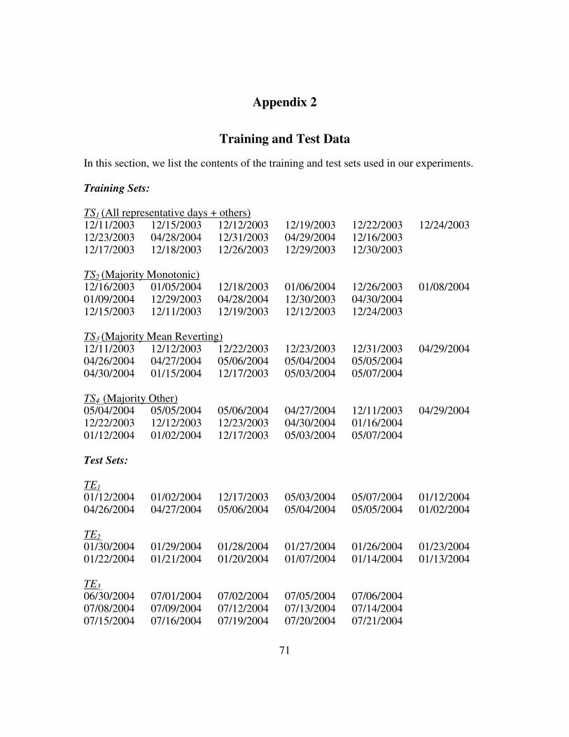
71
Appendix 2
Training and Test Data
In this section, we list the contents of the training and test sets used in our experiments. Training Sets: TS1 (All representative days + others) 12/11/2003 12/15/2003 12/12/2003 12/19/2003 12/22/2003 12/24/2003 12/23/2003 04/28/2004 12/31/2003 04/29/2004 12/16/2003 12/17/2003 12/18/2003 12/26/2003 12/29/2003 12/30/2003 TS2 (Majority Monotonic) 12/16/2003 01/05/2004 12/18/2003 01/06/2004 12/26/2003 01/08/2004 01/09/2004 12/29/2003 04/28/2004 12/30/2003 04/30/2004 12/15/2003 12/11/2003 12/19/2003 12/12/2003 12/24/2003 TS3 (Majority Mean Reverting) 12/11/2003 12/12/2003 12/22/2003 12/23/2003 12/31/2003 04/29/2004 04/26/2004 04/27/2004 05/06/2004 05/04/2004 05/05/2004 04/30/2004 01/15/2004 12/17/2003 05/03/2004 05/07/2004 TS4 (Majority Other) 05/04/2004 05/05/2004 05/06/2004 04/27/2004 12/11/2003 04/29/2004 12/22/2003 12/12/2003 12/23/2003 04/30/2004 01/16/2004 01/12/2004 01/02/2004 12/17/2003 05/03/2004 05/07/2004 Test Sets: TE1 01/12/2004 01/02/2004 12/17/2003 05/03/2004 05/07/2004 01/12/2004 04/26/2004 04/27/2004 05/06/2004 05/04/2004 05/05/2004 01/02/2004 TE2 01/30/2004 01/29/2004 01/28/2004 01/27/2004 01/26/2004 01/23/2004 01/22/2004 01/21/2004 01/20/2004 01/07/2004 01/14/2004 01/13/2004 TE3 06/30/2004 07/01/2004 07/02/2004 07/05/2004 07/06/2004 07/08/2004 07/09/2004 07/12/2004 07/13/2004 07/14/2004 07/15/2004 07/16/2004 07/19/2004 07/20/2004 07/21/2004

72
Appendix 3
Live Competition Results – April 2004 (http://www.cis.upenn.edu/~mkearns/projects/0507corrected.htm)
Days of test: 04/26/2004 05/03/2004 04/27/2004 05/04/2004 04/28/2004 05/05/2004 04/29/2004 05/06/2004 04/30/2004 05/07/2004 Trading agents were split into two groups: Red Pool and Blue Pool. Below are the final results over the two trading weeks.
RED POOL Agent Name Sharpe Ratio
ggc14 0.8334 hariharan -0.1619 kenyon 1.1221
lkt -0.4232 henis* -12.6200
* This agent was a VWAP agent and evaluated differently
BLUE POOL Agent Name Sharpe Ratio
lo 0.7213 ramamoorthy 2.4963
sherstov 0.7559 subramanian 0.5778
wu 0.0432 henis* -12.5931
* This agent was a VWAP agent and evaluated differently
The agent subramanian in the Blue Pool above is the GAA agent in the thesis.
73
References
[1] Neely C, Weller P and Dittmar R, Is technical analysis in the foreign exchange
market profitable? A genetic programming approach, Journal of Financial
Quantitative Analysis, Vol. 32, pp 405–26, 1997.
[2] Cohen J, Zinbarg E, Zeikel A, Investment Analysis and Portfolio Management,
McGraw-Hill, 1986.
[3] Lewis C, The Day Trader’s Guide to Technical Analysis, McGraw Hill, 2000.
[4] Murphy J J, Technical Analysis of the Financial Markets: A Comprehensive
Guide to Trading Methods & Applications, PHI, 1999.
[5] Tradetrek Homepage: http://www.tradetrek.com
[6] Schwager J, Technical Analysis, Wiley 1996.
[7] Bauer R J, Dahlquist J R, Technical Market Indicators: Analysis & Performance,
Wiley, 1998.
[8] Fang Y, Xu D, The Predictability of Asset Returns: an approach combining
technical analysis and time series forecasting, International Journal of
Forecasting, 2002.
[9] Kauffman P, Trading Systems and Methods, Wiley, 1998.
[10] Class Projects from CS395T: Agent Based E-Commerce at UT Austin
(http://www.cs.utexas.edu/users/pstone/Courses/395Tfall03/resources/index.html)
(a) Ramamoorthy S, A Strategy for Stock Trading based on Multiple Models and
trading rules.
(b) Sherstov A, Automated Stock Trading in PLAT.
(c) Subramanian H, Automated PLAT Trading Agent using Order Imbalance in
Volume.
[11] Greenwald A, Jennings N R, Stone P, Agents and Markets, Guest Editor’s
Introduction, 18(6), Nov/Dec 2003
[12] Tino P, Schittenkopf C, Dorffner G, Financial Volatility Trading using Recurrent
Neural Networks, IEEE Transactions on Neural Networks, 12(4), 2001.
74
[13] Wah B W, Qian M, Constrained Formulations and Algorithms for Stock
Predictions using Recurrent FIR Neural Networks, AAAI/IAAI, 2002.
[14] Dunis C and Zhou B, Nonlinear Modeling of High Frequency Financial Time
Series, Wiley 1998.
[15] Deboeck G (ed), Trading on the Edge: Neural, Genetic and Fuzzy Systems for
Chaotic Financial Markets, Wiley, 1994.
[16] E. F. Fama, Random Walks in Stock Market Prices, Financial Analysts Journal,
September/October 1965 (reprinted January-February 1995).
[17] Patrick S, Trading Volume and Autocorrelation: Empirical Evidence from the
Stockholm Stock Exchange, Stockholm School of Economics, 1997.
[18] Malkiel B, A Random Walk Down Wall Street, WW.Norton, 1996.
[19] Kearns M, Ortiz L, The Penn-Lehman Automated Trading project, IEEE
Intelligent Systems, 18(6), pp 22 – 31, Nov/Dec 2003.
[20] Hellstrom T, Holmstrom K, Parameter Tuning in Trading Algorithms using
ASTA, Computational Finance, pages 343-357, Cambridge, MA, MIT Press, 1999.
[21] Dunis C et al., Optimizing Intraday Trading Models with Genetic Algorithms,
Working Paper, Liverpool Business School, 1999.
[22] Island ECN: http://www.island.com
[23] Hennessey S, Using an In-Class Simulation to teach Financial Markets, Working
Paper, University of Prince Edward Island, 1998.
[24] Fincoach.com Website: http://fincoach.com
[25] LeBaron B, Building the Santa Fe Artificial Stock Market, Working Paper,
Brandeis University, 2002.
[26] Brock W, Lakonishok J, LeBaron B, Simple technical trading rules and the
stochastic properties of stock returns, Journal of Finance, 47(5), pp, Dec 1992.
[27] Resistance & Support Reference:
http://www.stockcharts.com/education/ChartAnalysis/supportResistance.html
[28] Refenes A P(ed.), Neural Networks in Capital Markets, Wiley 1995.
[29] Pictet O et al., Real-time trading models for foreign exchange rates, Neural
Network World Volume 6, 713–44, 1992.
75
[30] Dempster M A H and Jones C M, A real-time adaptive trading system using
genetic programming, Quantitative Finance Vol. 1, Institute of Physics
Publishing, pp 397- 413, 2001.
[31] Mitchell M, An Introduction to Genetic Algorithms, MIT Press, 1996.
[32] Bauer R J, Genetic Algorithms and Investment Strategies, Wiley 1994.
[33] Stock Market Game website: http://www.smgww.org
[34] Virtual Stock Exchange website: http://www.virtualstockexchange.com
[35] Dempster M A H, Jones C M, Can Technical Pattern Trading be Profitably
Automated, Working Paper, Judge Institutes of Management Studies, 1999.
[36] Li J, Tsang E P K, Improving Technical Analysis Predictions: An Application of
Genetic Programming, Proceedings of Florida Artificial Intelligence Research
Symposium, 1999.
[37] Oussaidene M, Chopard B, Pictet O V, Tomassini M, Parallel Genetic
Programming and its application to Trading Model Induction, Parallel
Computing, Vol 23, 1997.
[38] Sherstov A, Stone P, Three Automated Stock Trading Agents: A Comparative
Study, AAMAS Workshop on Agent Mediated Electronic Commerce – VI, 2004.
[39] Gomes F, Portfolio Choice and Trading Volume with Loss-Averse Investors,
London Business School, 2003.
[40] Allen F, Karjalainen R, Using genetic algorithms to find technical trading rules,
J. Financial Economics, Vol.51, pp 245 – 271, 1999.
[41] Holland J H, Adaptation in Natural and Artificial Systems, University of
Michigan Press, Ann Arbor, 1975.
[42] Koza J R, Genetic Programming: On the Programming of Computers by means of
Natural Selection, MIT Press, 1992.
[43] Papagelis A, Kalles D, GA Tree: Genetically Evolved Decision Trees, ICTAI,
2000.
[44] Dempster M A H, Payne T W, Romahi Y, Thompson G W P, Computational
Learning Techniques for Intraday FX Trading Using Popular Technical
Indicators, IEEE Transactions on Neural Networks, 12(4), 2001.
76
[45] Sharpe W F, Mutual Fund Performance, Journal of Business, January 1966.
[46] Pendersen C S, Derivatives and Downside Risk. Derivatives Use, Trading and
Regulation, 2001.
[47] Littlestone N, Warmuth M K, The Weighted Majority Algorithm, University of
California, Santa Cruz, 1992.
[48] Feng Y, Yu R, Stone P, Two Stock Trading Agents: Market Making and Technical
Analysis, Dept. of Computer Sciences, UT Austin.
[49] Chordia T, Subrahmanyam A, Order Imbalance and Individual Stock Returns,
Emory University, University of California, Los Angeles, 2002.
[50] PLAT website: http://www.cis.upenn.edu/~mkearns/projects/pat.html.
[51] Hariharan G, News Mining Agent for Automated Stock Trading, Thesis,
University of Texas, Austin, 2004.
[52] Yahoo! Finance Website: http://finance.yahoo.com/ [53] Bollinger Bands Website: http://www.bollingerbands.com/ [54] Genetic Algorithm Pseudo code: http://www.cs.bgu.ac.il/~sipper/ga.html

77
Vita
Harish K Subramanian was born on April 3, 1981, the son of Lakshmi
Subramanian and Ramamoorthy Subramanian. After completing his work at Choithram
School, Indore, India, in 1998, he entered R.V. College of Engineering, Bangalore, India.
He received the degree of Bachelor of Engineering in Instrumentation Technology from
Visveswaraiah Technological University in July 2002. He entered The Graduate School
at The University of Texas at Austin in August 2002.
Permanent address: A3/23 Gagan Apts, 2 Cross, Atmananda Colony,
Sultanpalya, Bangalore 560 032, India.
This thesis was typed by the author.