Copyright ©2014 Pearson Education Chap 4-1 Chapter 4 Basic Probability Statistics for Managers Using Microsoft Excel 7 th Edition, Global Edition

Copyright ©2014 Pearson Education Chap 4-1

Chapter 4

Basic Probability

Statistics for Managers Using Microsoft Excel

7th Edition, Global Edition


Learning Objectives

In this chapter, you learn:

Basic probability concepts Conditional probability To use Bayes’ Theorem to revise probabilities


Basic Probability Concepts

Probability – the chance that an uncertain event will occur (always between 0 and 1)

Impossible Event – an event that has no chance of occurring (probability = 0)

Certain Event – an event that is sure to occur (probability = 1)


Assessing Probability

There are three approaches to assessing the probability of an uncertain event:

1. a priori -- based on prior knowledge of the process

2. empirical probability

3. subjective probability

outcomeselementaryofnumbertotal

occurcaneventthewaysofnumber

T

X

based on a combination of an individual’s past experience, personal opinion, and analysis of a particular situation


occurcaneventthewaysofnumber

Assuming all outcomes are equally likely

probability of occurrence

probability of occurrence


Example of a priori probability

When randomly selecting a day from the year 2013 what is the probability the day is in January?

2013 in days ofnumber total

January in days ofnumber January In Day of yProbabilit

T

X

365

31

2013 in days 365

January in days 31

T

X


Example of empirical probability

Taking Stats Not Taking Stats

Total

Male 84 145 229

Female 76 134 210

Total 160 279 439

Find the probability of selecting a male taking statistics from the population described in the following table:

191.0439

84

people ofnumber total

stats takingmales ofnumber Probability of male taking stats

Copyright ©2014 Pearson Education

Subjective probability

Subjective probability may differ from person to person A media development team assigns a 60%

probability of success to its new ad campaign. The chief media officer of the company is less

optimistic and assigns a 40% of success to the same campaign

The assignment of a subjective probability is based on a person’s experiences, opinions, and analysis of a particular situation

Subjective probability is useful in situations when an empirical or a priori probability cannot be computed

Chap 4-7


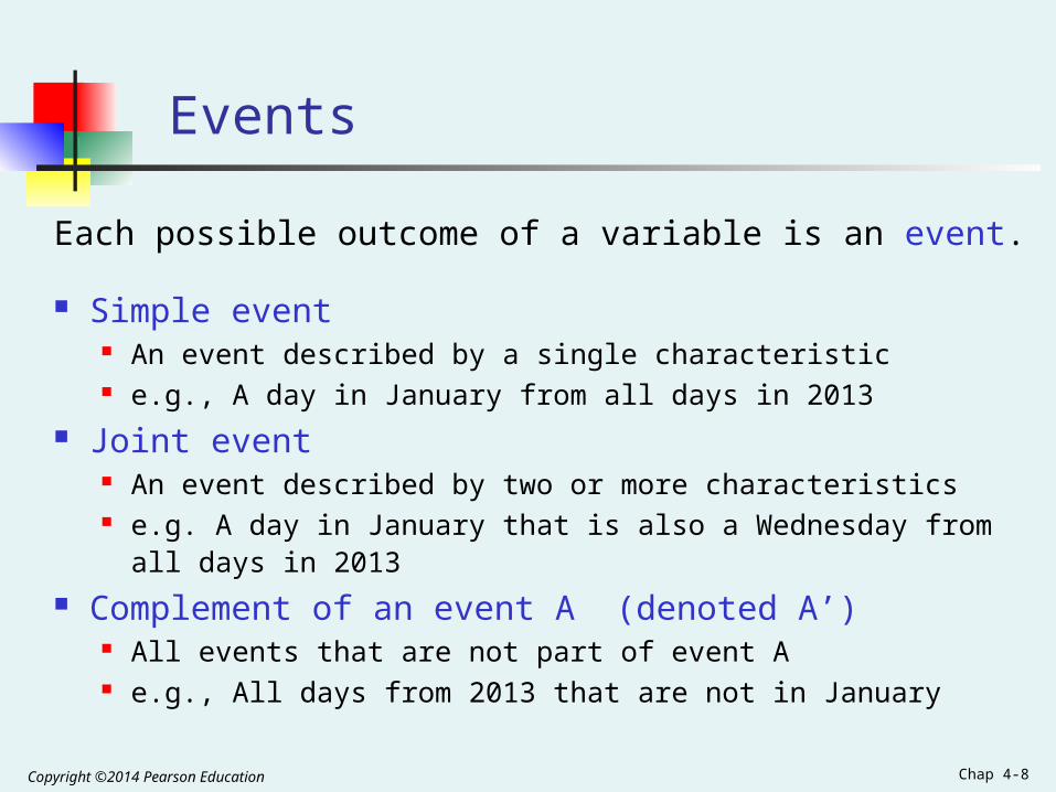
Events

Each possible outcome of a variable is an event.

Simple event An event described by a single characteristic e.g., A day in January from all days in 2013

Joint event An event described by two or more characteristics e.g. A day in January that is also a Wednesday from all days in 2013

Complement of an event A (denoted A’) All events that are not part of event A e.g., All days from 2013 that are not in January


Sample Space

The Sample Space is the collection of all possible events

e.g. All 6 faces of a die:

e.g. All 52 cards of a bridge deck:


Organizing & Visualizing Events

Contingency Tables -- For All Days in 2013

Decision Trees

All Days

In 2013 Not Jan.

Jan.

Not Wed.

Wed.

Wed.

Not Wed.

Sample Space

TotalNumberOfSampleSpaceOutcomes

Not Wed. 27 286 313

Wed. 5 47 52

Total 32 333 365

Jan. Not Jan. Total

5

27

47

286


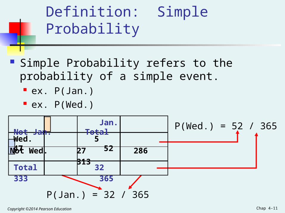
Definition: Simple Probability

Simple Probability refers to the probability of a simple event. ex. P(Jan.) ex. P(Wed.)

P(Jan.) = 32 / 365

P(Wed.) = 52 / 365

Not Wed. 27 286 313

Wed. 5 47 52

Total 32 333 365

Jan. Not Jan. Total


Definition: Joint Probability

Joint Probability refers to the probability of an occurrence of two or more events (joint event). ex. P(Jan. and Wed.) ex. P(Not Jan. and Not Wed.)

P(Jan. and Wed.) = 5 / 365

P(Not Jan. and Not Wed.)= 286 / 365

Not Wed. 27 286 313

Wed. 5 47 52

Total 32 333 365

Jan. Not Jan. Total


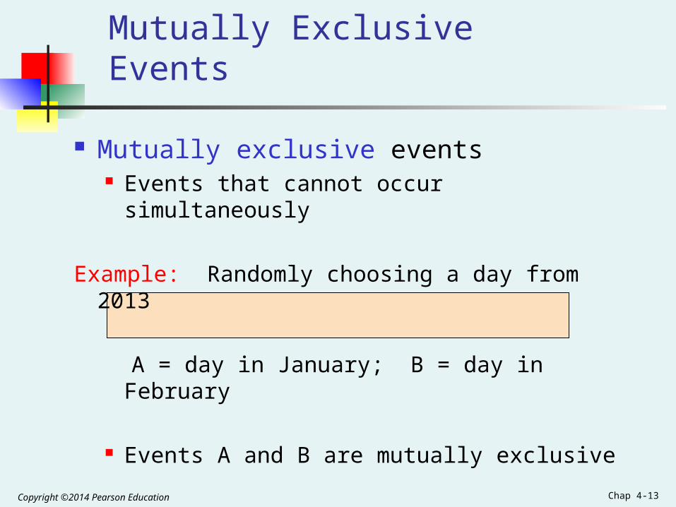
Mutually Exclusive Events

Mutually exclusive events Events that cannot occur simultaneously

Example: Randomly choosing a day from 2013

A = day in January; B = day in February

Events A and B are mutually exclusive


Collectively Exhaustive Events

Collectively exhaustive events One of the events must occur The set of events covers the entire sample space

Example: Randomly choose a day from 2013

A = Weekday; B = Weekend; C = January; D = Spring;

Events A, B, C and D are collectively exhaustive (but not mutually exclusive – a weekday can be in January or in Spring)

Events A and B are collectively exhaustive and also mutually exclusive


Computing Joint and Marginal Probabilities

The probability of a joint event, A and B:

Computing a marginal (or simple) probability:

Where B1, B2, …, Bk are k mutually exclusive and collectively exhaustive events


BandAsatisfyingoutcomesofnumber)BandA(P

)BdanP(A)BandP(A)BandP(AP(A) k21


Joint Probability Example

P(Jan. and Wed.)

365

5

2013in days ofnumber total

Wed.are and Jan.in are that days ofnumber

Not Wed. 27 286 313

Wed. 5 47 52

Total 32 333 365

Jan. Not Jan. Total


Marginal Probability Example

P(Wed.)

365

52

365

48

365

4)Wed.andJan.P(Not Wed.)andJan.( P

Not Wed. 27 286 313

Wed. 4 48 52

Total 31 334 365

Jan. Not Jan. Total


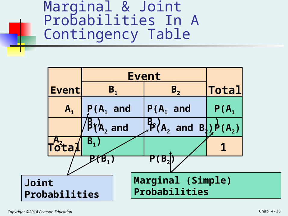
P(A1 and B2) P(A1)

TotalEvent

Marginal & Joint Probabilities In A Contingency Table

P(A2 and B1)

P(A1 and B1)

Event

Total 1

Joint Probabilities Marginal (Simple) Probabilities

A1

A2

B1 B2

P(B1) P(B2)

P(A2 and B2) P(A2)


Probability Summary So Far

Probability is the numerical measure of the likelihood that an event will occur

The probability of any event must be between 0 and 1, inclusively

The sum of the probabilities of all mutually exclusive and collectively exhaustive events is 1

Certain

Impossible

0.5

1

0

0 ≤ P(A) ≤ 1 For any event A

1P(C)P(B)P(A) If A, B, and C are mutually exclusive and collectively exhaustive


General Addition Rule

P(A or B) = P(A) + P(B) - P(A and B)

General Addition Rule:

If A and B are mutually exclusive, then

P(A and B) = 0, so the rule can be simplified:

P(A or B) = P(A) + P(B)

For mutually exclusive events A and B


General Addition Rule Example

P(Jan. or Wed.) = P(Jan.) + P(Wed.) - P(Jan. and Wed.)

= 32/365 + 52/365 - 5/365 = 79/365Don’t count the five Wednesdays in January twice!

Not Wed. 27 286 313

Wed. 5 47 52

Total 32 333 365

Jan. Not Jan. Total


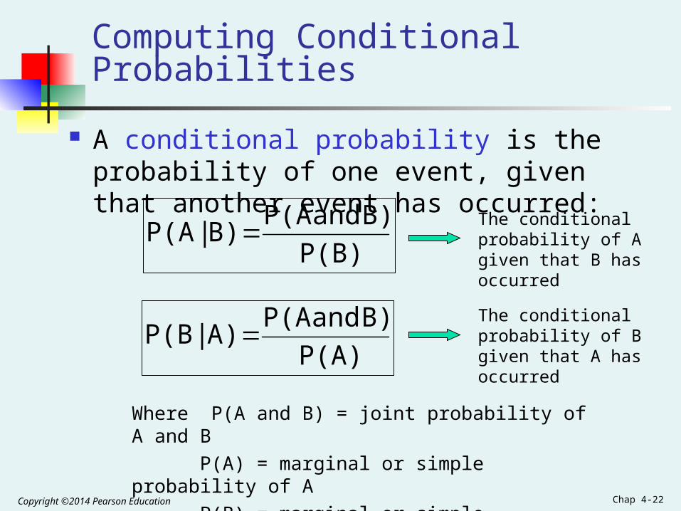
Computing Conditional Probabilities

A conditional probability is the probability of one event, given that another event has occurred:

P(B)

B)andP(AB)|P(A

P(A)

B)andP(AA)|P(B

Where P(A and B) = joint probability of A and B

P(A) = marginal or simple probability of A

P(B) = marginal or simple probability of B

The conditional probability of A given that B has occurred

The conditional probability of B given that A has occurred


What is the probability that a car has a GPS, given that it has AC ?

i.e., we want to find P(GPS | AC)

Conditional Probability Example

Of the cars on a used car lot, 70% have air conditioning (AC) and 40% have a GPS. 20% of the cars have both.


No GPSGPS Total

AC 0.2 0.5 0.7

No AC 0.2 0.1 0.3

Total 0.4 0.6 1.0

Of the cars on a used car lot, 70% have air conditioning (AC) and 40% have a GPS and 20% of the cars have both.

0.28570.7

0.2

P(AC)

AC)andP(GPSAC)|P(GPS

(continued)



No GPSGPS Total

AC 0.2 0.5 0.7

No AC 0.2 0.1 0.3

Total 0.4 0.6 1.0

Given AC, we only consider the top row (70% of the cars). Of these, 20% have a GPS. 20% of 70% is about 28.57%.

0.28570.7

0.2

P(AC)

AC)andP(GPSAC)|P(GPS

(continued)



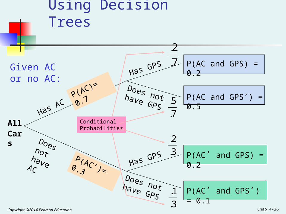
Using Decision Trees

Has AC

Does not have AC

Has GPS

Does not have GPS

Has GPS

Does not have GPS

P(AC)= 0.7

P(AC’)= 0.3

P(AC and GPS) = 0.2

P(AC and GPS’) = 0.5

P(AC’ and GPS’) = 0.1

P(AC’ and GPS) = 0.2

7.

5.

3.

2.

3.

1.

AllCars

7.

2.

Given AC or no AC:

ConditionalProbabilities


Has GPS

Does not have GPS

Has AC

Does not have AC

Has AC

Does not have AC

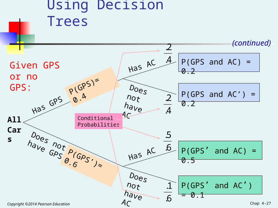
P(GPS)= 0.4

P(GPS’)= 0.6

P(GPS and AC) = 0.2

P(GPS and AC’) = 0.2

P(GPS’ and AC’) = 0.1

P(GPS’ and AC) = 0.5

4.

2.

6.

5.

6.

1.

AllCars

4.

2.

Given GPS or no GPS:

(continued)

ConditionalProbabilities

Using Decision Trees


Independence

Two events are independent if and only if:

Events A and B are independent when the probability of one event is not affected by the fact that the other event has occurred

P(A)B)|P(A


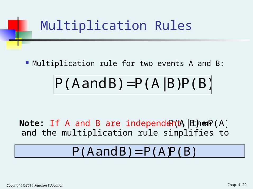
Multiplication Rules

Multiplication rule for two events A and B:

P(B)B)|P(AB)andP(A

P(A)B)|P(A Note: If A and B are independent, thenand the multiplication rule simplifies to

P(B)P(A)B)andP(A


Marginal Probability

Marginal probability for event A:

Where B1, B2, …, Bk are k mutually exclusive and collectively exhaustive events

)P(B)B|P(A)P(B)B|P(A)P(B)B|P(A P(A) kk2211


Bayes’ Theorem

Bayes’ Theorem is used to revise previously calculated probabilities based on new information.

Developed by Thomas Bayes in the 18th Century.

It is an extension of conditional probability.


where:

Bi = ith event of k mutually exclusive and collectively

exhaustive events

A = new event that might impact P(Bi)

))P(BB|P(A))P(BB|P(A))P(BB|P(A

))P(BB|P(AA)|P(B

k k 2 2 1 1

i i i

Bayes’ Theorem


Bayes’ Theorem Example

A drilling company has estimated a 40% chance of striking oil for their new well.

A detailed test has been scheduled for more information. Historically, 60% of successful wells have had detailed tests, and 20% of unsuccessful wells have had detailed tests.

Given that this well has been scheduled for a detailed test, what is the probability

that the well will be successful?


Let S = successful well

U = unsuccessful well P(S) = 0.4 , P(U) = 0.6 (prior probabilities)

Define the detailed test event as D

Conditional probabilities:

P(D|S) = 0.6 P(D|U) = 0.2

Goal is to find P(S|D)

(continued)



0.6670.120.24

0.24

(0.2)(0.6)(0.6)(0.4)

(0.6)(0.4)

U)P(U)|P(DS)P(S)|P(D

S)P(S)|P(DD)|P(S

(continued)

Apply Bayes’ Theorem:

So the revised probability of success, given that this well has been scheduled for a detailed test, is 0.667



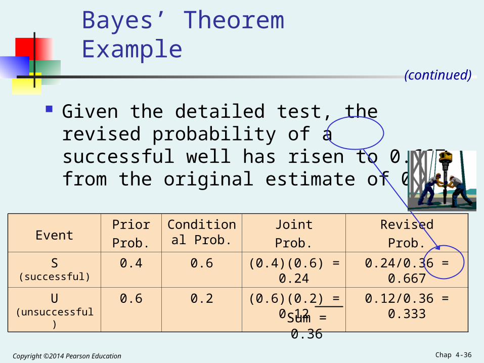
Given the detailed test, the revised probability of a successful well has risen to 0.667 from the original estimate of 0.4

EventPrior

Prob.

Conditional Prob.

Joint

Prob.

Revised

Prob.

S (successful) 0.4 0.6 (0.4)(0.6) = 0.24 0.24/0.36 = 0.667

U (unsuccessful) 0.6 0.2 (0.6)(0.2) = 0.12 0.12/0.36 = 0.333

Sum = 0.36

(continued)



Counting Rules Are Often Useful In Computing Probabilities

Counting rules are covered as an on-line topic

Chap 4-37


Chapter Summary

In this chapter we discussed:

Basic probability concepts Sample spaces and events, contingency tables, simple

probability, and joint probability

Basic probability rules General addition rule, addition rule for mutually exclusive events,

rule for collectively exhaustive events

Conditional probability Statistical independence, marginal probability, decision trees,

and the multiplication rule

Bayes’ theorem

Copyright ©2014 Pearson Education Counting Rules - 1

Online Topic

Counting Rules

Statistics for Managers using Microsoft Excel

7th Edition

Copyright ©2014 Pearson Education Counting Rules -2

Learning Objective

In many cases, there are a large number of possible outcomes.

In this topic, you learn various counting rules for such situations.

Copyright ©2014 Pearson Education Counting Rules -3

Counting Rules

Rules for counting the number of possible outcomes

Counting Rule 1: If any one of k different mutually exclusive and

collectively exhaustive events can occur on each of n trials, the number of possible outcomes is equal to

Example If you roll a fair die 3 times then there are 63 = 216 possible

outcomes

kn


Counting Rule 2: If there are k1 events on the first trial, k2 events on

the second trial, … and kn events on the nth trial, the number of possible outcomes is

Example: You want to go to a park, eat at a restaurant, and see a

movie. There are 3 parks, 4 restaurants, and 6 movie choices. How many different possible combinations are there?

Answer: (3)(4)(6) = 72 different possibilities

(k1)(k2)…(kn)

(continued)

Counting Rules


Counting Rule 3: The number of ways that n items can be arranged in

order is

Example: You have five books to put on a bookshelf. How many

different ways can these books be placed on the shelf?

Answer: 5! = (5)(4)(3)(2)(1) = 120 different possibilities

n! = (n)(n – 1)…(1)

(continued)

Counting Rules


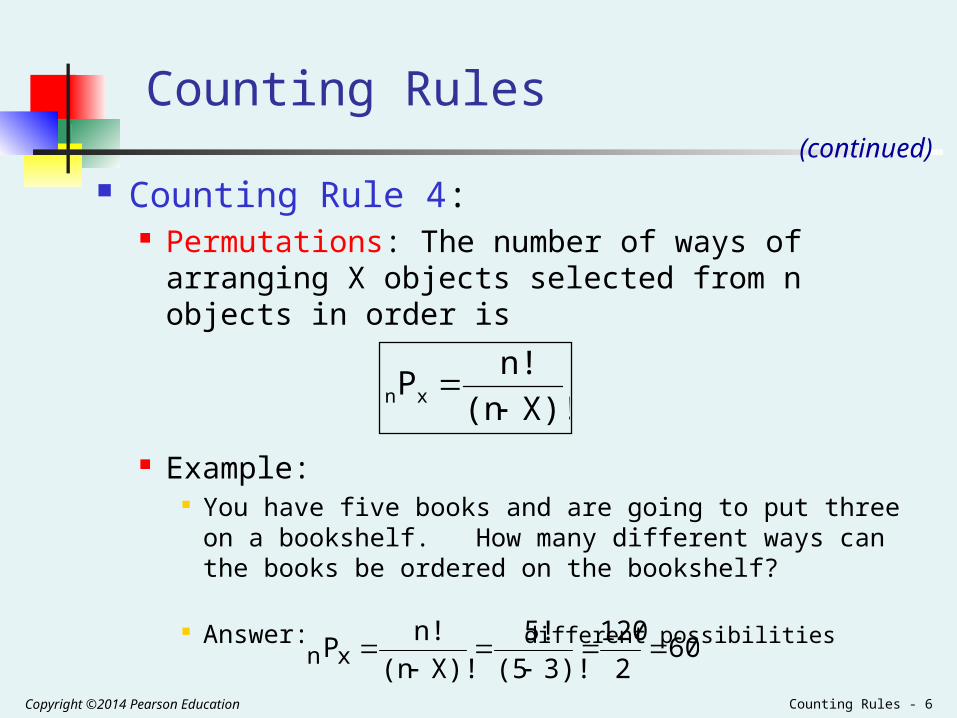
Counting Rule 4: Permutations: The number of ways of arranging X

objects selected from n objects in order is

Example: You have five books and are going to put three on a

bookshelf. How many different ways can the books be ordered on the bookshelf?

Answer: different

possibilities

(continued)

X)!(n

n!Pxn

602

120

3)!(5

5!

X)!(n

n!Pxn

Counting Rules


Counting Rule 5: Combinations: The number of ways of selecting X

objects from n objects, irrespective of order, is

Example: You have five books and are going to select three are to

read. How many different combinations are there, ignoring the order in which they are selected?

Answer: different possibilities

(continued)

X)!(nX!

n!Cxn

10(6)(2)

120

3)!(53!

5!

X)!(nX!

n!Cxn

Counting Rules


Topic Summary

In this topic we examined

Five useful counting rules


All rights reserved. No part of this publication may be reproduced, stored in a retrieval system, or transmitted, in any form or by any means, electronic, mechanical, photocopying, recording, or

otherwise, without the prior written permission of the publisher. Printed in the United States of America.

Documents

Copyright ©2014 Pearson Education Chap 4-1 Chapter 4 Basic Probability Statistics for Managers Using Microsoft Excel 7 th Edition, Global Edition