Embed Size (px)
Citation preview
Chap 4-1
Statistics
Please Stand By….
Chap 4-2
Chapter 4: Probability and Distributions
Randomness General Probability Probability Models Random Variables Moments of Random Variables
Chap 4-3
Randomness
The language of probability
Thinking about randomness
The uses of probability
Chap 4-4
Randomness

Chap 4-5
Randomness
Chap 4-6
Randomness
Chap 4-7
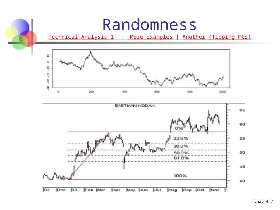
RandomnessTechnical Analysis 1 | More Examples | Another (Tipping Pts)
Chap 4-8
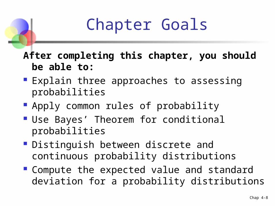
Chapter Goals
After completing this chapter, you should be able to:
Explain three approaches to assessing probabilities
Apply common rules of probability Use Bayes’ Theorem for conditional probabilities Distinguish between discrete and continuous
probability distributions Compute the expected value and standard
deviation for a probability distributions
Chap 4-9
Important Terms
Probability – the chance that an uncertain event will occur (always between 0 and 1)
Experiment – a process of obtaining outcomes for uncertain events
Elementary Event – the most basic outcome possible from a simple experiment
Randomness – Does not mean haphazard Description of the kind of order that emerges only in
the long run
Chap 4-10
Important Terms (CONT’D)
Sample Space – the collection of all possible elementary outcomes
Probability Distribution Function Maps events to intervals on the real line Discrete probability mass Continuous probability density
Chap 4-11
Sample Space
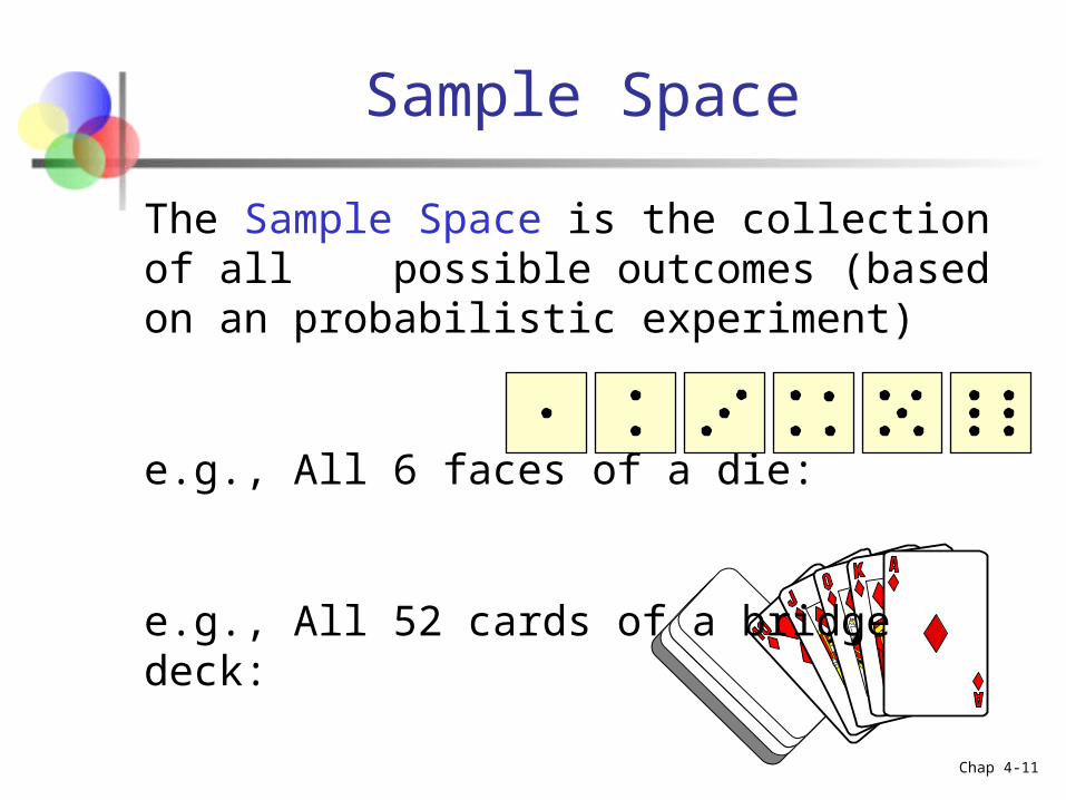
The Sample Space is the collection of all possible outcomes (based on an probabilistic experiment)
e.g., All 6 faces of a die:
e.g., All 52 cards of a bridge deck:
Chap 4-12
Events
Elementary event – An outcome from a sample space with one characteristic Example: A red card from a deck of cards
Event – May involve two or more outcomes simultaneously Example: An ace that is also red from a deck
of cards
Chap 4-13
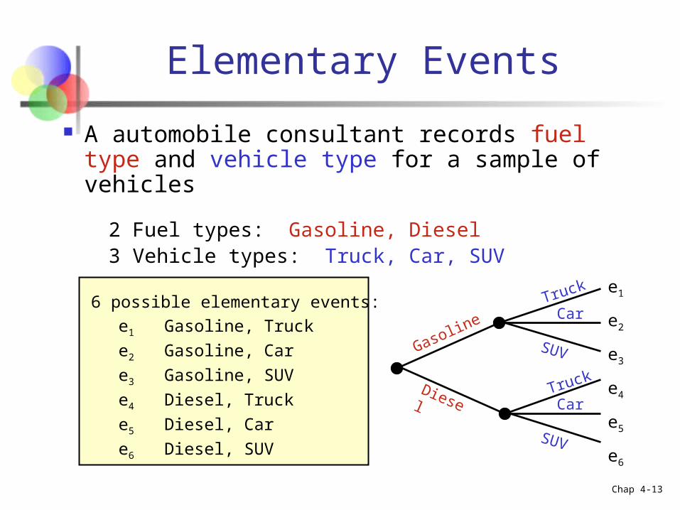
Elementary Events
A automobile consultant records fuel type and vehicle type for a sample of vehicles
2 Fuel types: Gasoline, Diesel3 Vehicle types: Truck, Car, SUV
6 possible elementary events:
e1 Gasoline, Truck
e2 Gasoline, Car
e3 Gasoline, SUV
e4 Diesel, Truck
e5 Diesel, Car
e6 Diesel, SUV
Gasoline
Diesel
CarTruck
Truck
Car
SUV
SUV
e1
e2
e3
e4
e5
e6
Chap 4-14
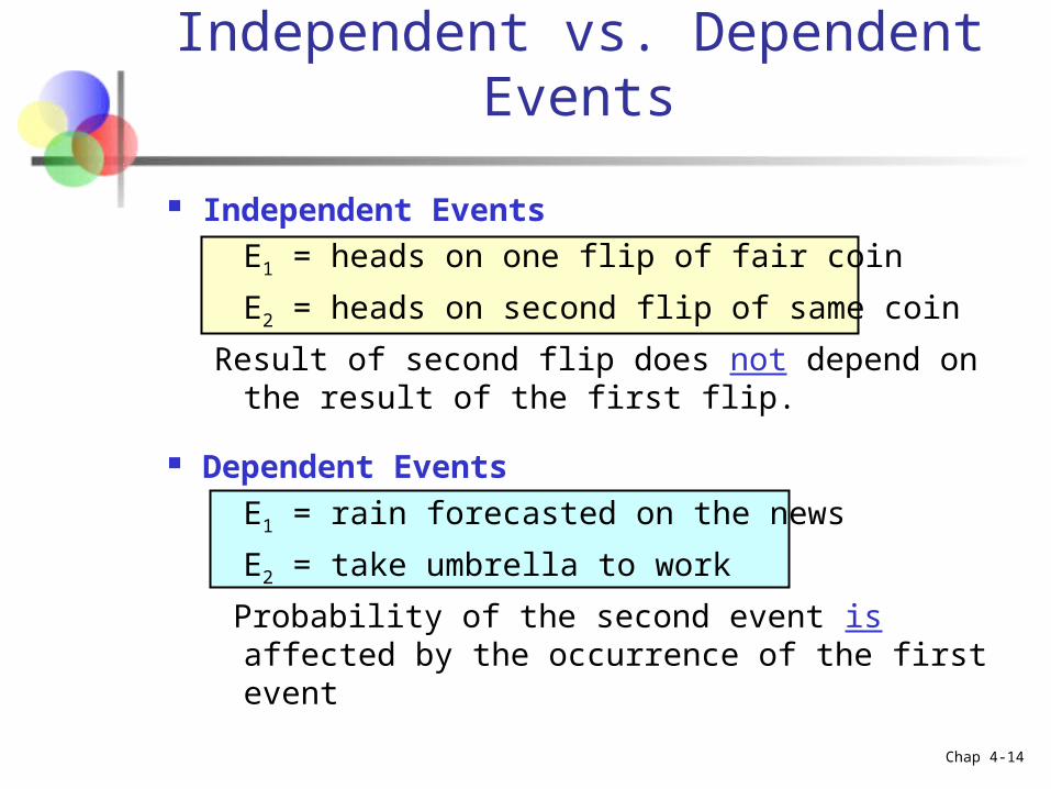
Independent Events
E1 = heads on one flip of fair coin
E2 = heads on second flip of same coin
Result of second flip does not depend on the result of the first flip.
Dependent Events
E1 = rain forecasted on the news
E2 = take umbrella to work
Probability of the second event is affected by the occurrence of the first event
Independent vs. Dependent Events
Chap 4-15
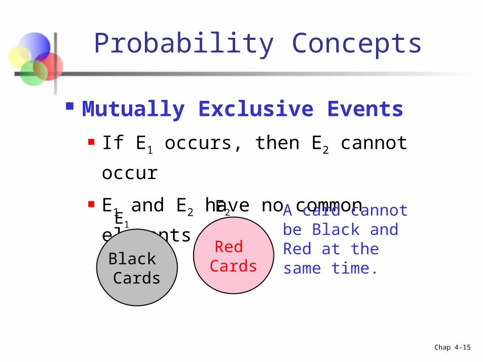
Probability Concepts
Mutually Exclusive Events If E1 occurs, then E2 cannot occur
E1 and E2 have no common elements
Black Cards
Red Cards
A card cannot be Black and Red at the same time.
E1
E2
Chap 4-16
Coming up with Probability
Empirically From the data! Based on observation, not theory
Probability describes what happens in very many trials.
We must actually observe many trials to pin down a probability
Based on belief (Bayesian Technique)
Chap 4-17
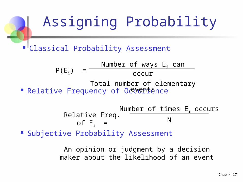
Assigning Probability
Classical Probability Assessment
Relative Frequency of Occurrence
Subjective Probability Assessment
P(Ei) =Number of ways Ei can occur
Total number of elementary events
Relative Freq. of Ei =Number of times Ei occurs
N
An opinion or judgment by a decision maker about the likelihood of an event
Chap 4-18
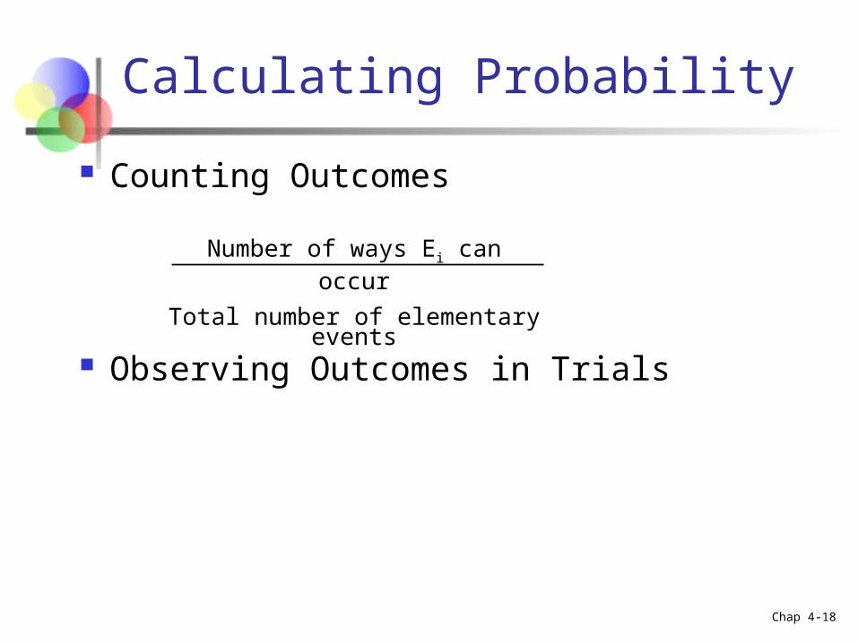
Calculating Probability
Counting Outcomes
Observing Outcomes in Trials
Number of ways Ei can occur
Total number of elementary events
Chap 4-19
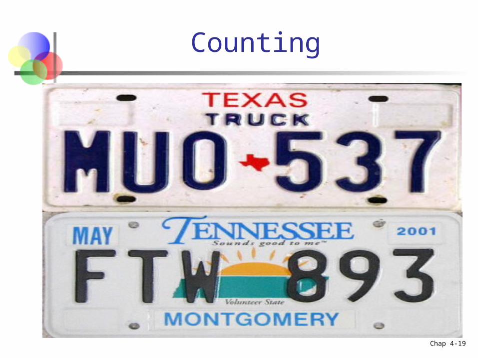
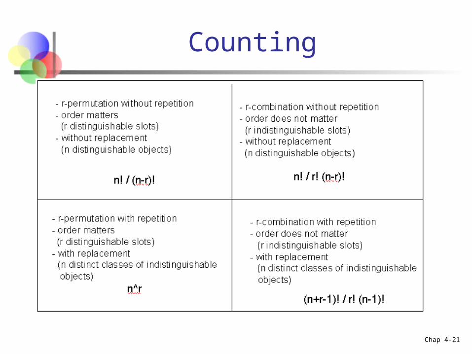
Counting
Chap 4-20
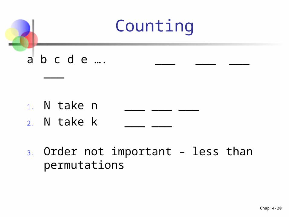
Counting
a b c d e …. ___ ___ ___ ___
1. N take n ___ ___ ___
2. N take k ___ ___
3. Order not important – less than permutations
Chap 4-21
Counting
Chap 4-22
Rules of Probability
S is sample space Pr(S) = 1 Events measured in numbers result in a
Probability Distribution
Chap 4-23
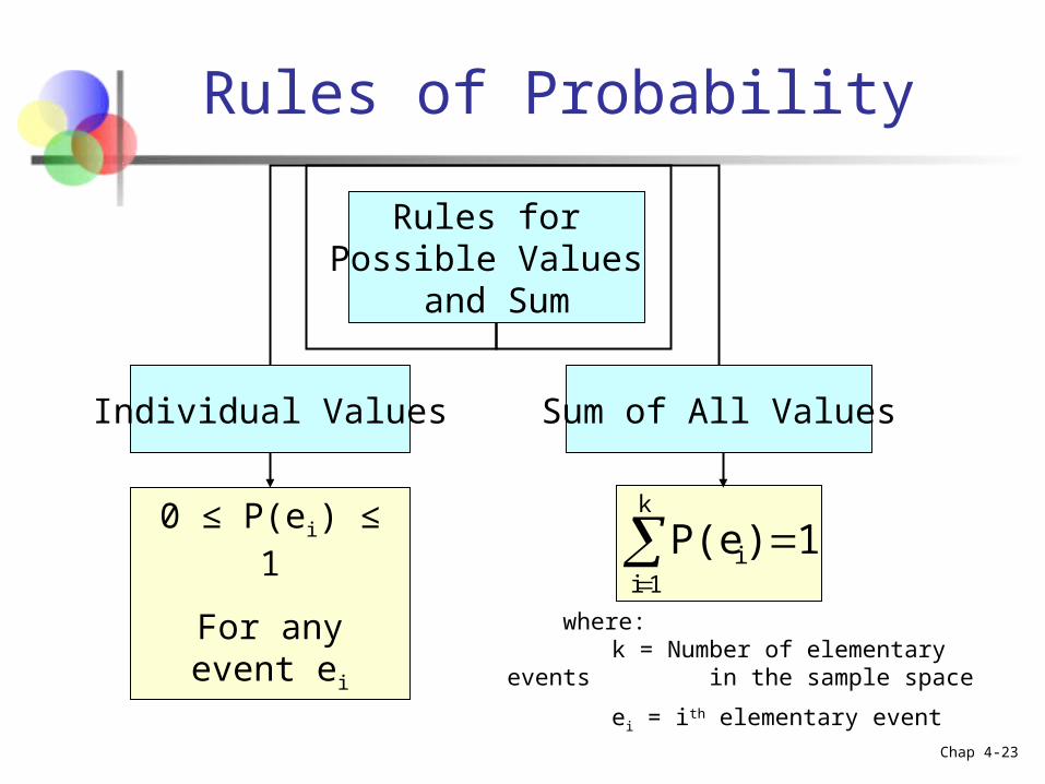
Rules of Probability
Rules for Possible Values
and Sum
Individual Values Sum of All Values
0 ≤ P(ei) ≤ 1
For any event ei
1)P(ek
1ii
where:k = Number of elementary events in the sample space
ei = ith elementary event
Chap 4-24
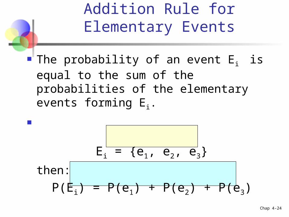
Addition Rule for Elementary Events
The probability of an event Ei is equal to the sum of the probabilities of the elementary events forming Ei.
That is, if:
Ei = {e1, e2, e3}
then:
P(Ei) = P(e1) + P(e2) + P(e3)
Chap 4-25
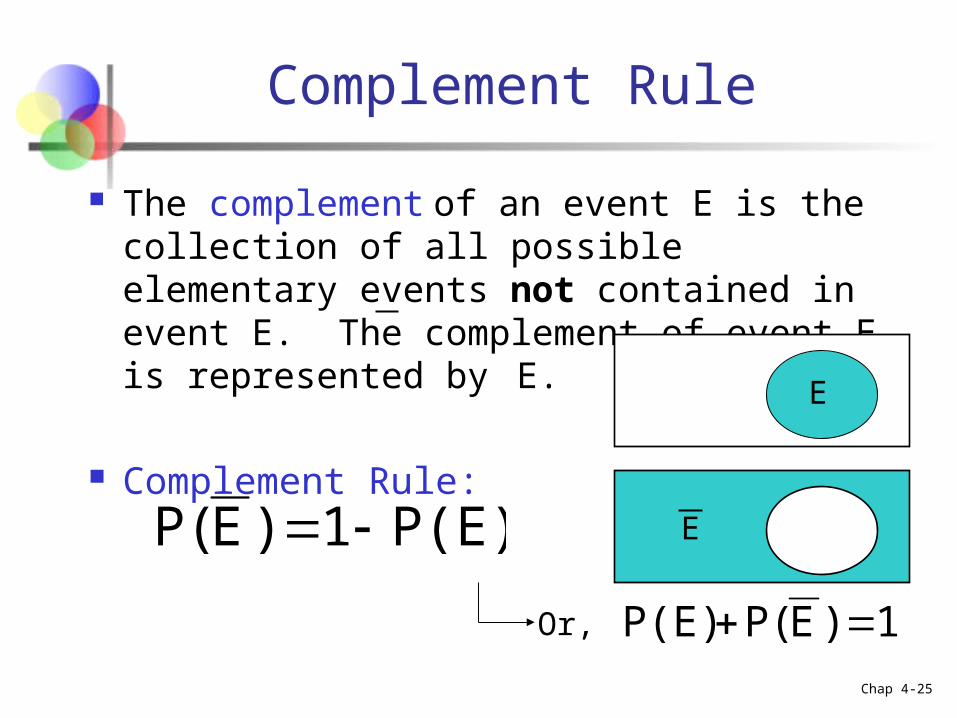
Complement Rule
The complement of an event E is the collection of all possible elementary events not contained in event E. The complement of event E is represented by E.
Complement Rule:
P(E)1)EP( E
E
1)EP(P(E) Or,
Chap 4-26
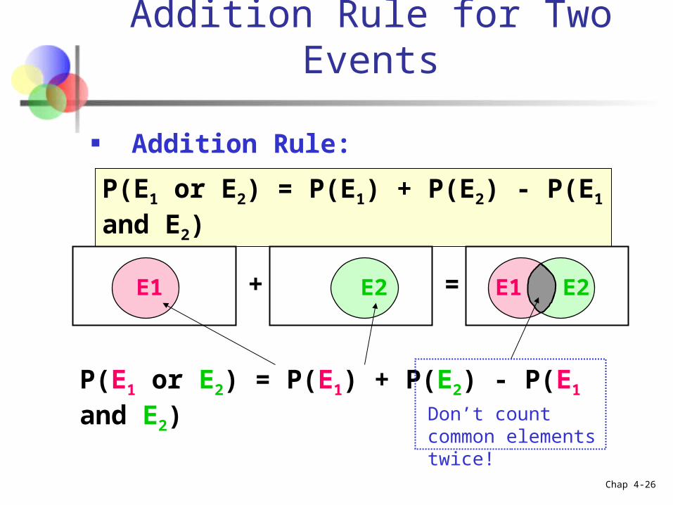
Addition Rule for Two Events
P(E1 or E2) = P(E1) + P(E2) - P(E1 and E2)
E1 E2
P(E1 or E2) = P(E1) + P(E2) - P(E1 and E2)Don’t count common elements twice!
■ Addition Rule:
E1 E2+ =
Chap 4-27
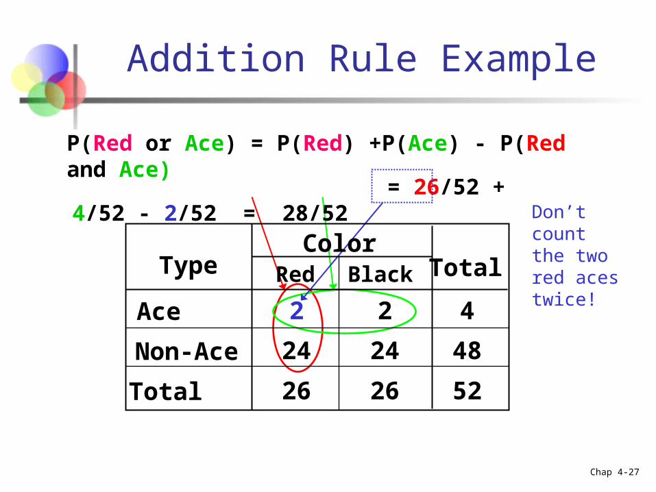
Addition Rule Example
P(Red or Ace) = P(Red) +P(Ace) - P(Red and Ace)
= 26/52 + 4/52 - 2/52 = 28/52Don’t count the two red aces twice!
BlackColor
Type Red Total
Ace 2 2 4
Non-Ace 24 24 48
Total 26 26 52
Chap 4-28
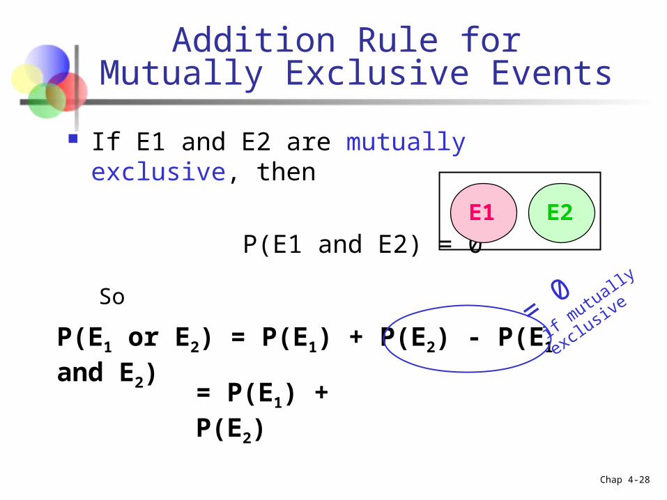
Addition Rule for Mutually Exclusive Events
If E1 and E2 are mutually exclusive, then
P(E1 and E2) = 0
So
P(E1 or E2) = P(E1) + P(E2) - P(E1 and E2)
= P(E1) + P(E2)
= 0
E1 E2
if mutually
exclusiv
e
Chap 4-29
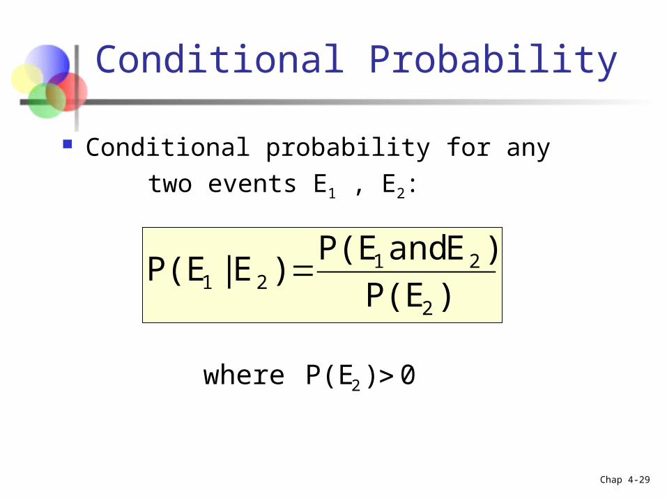
Conditional Probability
Conditional probability for any
two events E1 , E2:
)P(E
)EandP(E)E|P(E
2
2121
0)P(Ewhere 2
Chap 4-30
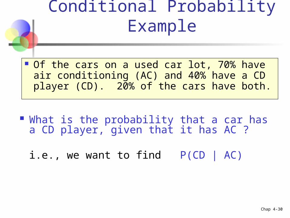
What is the probability that a car has a CD player, given that it has AC ?
i.e., we want to find P(CD | AC)
Conditional Probability Example
Of the cars on a used car lot, 70% have air conditioning (AC) and 40% have a CD player (CD). 20% of the cars have both.
Chap 4-31
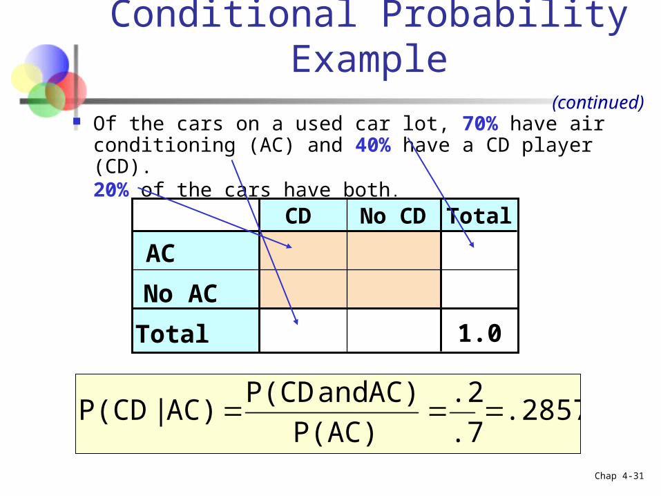
Conditional Probability Example
No CDCD Total
AC
No AC
Total 1.0
Of the cars on a used car lot, 70% have air conditioning (AC) and 40% have a CD player (CD). 20% of the cars have both.
.2857.7
.2
P(AC)
AC)andP(CDAC)|P(CD
(continued)
Chap 4-32
Conditional Probability Example
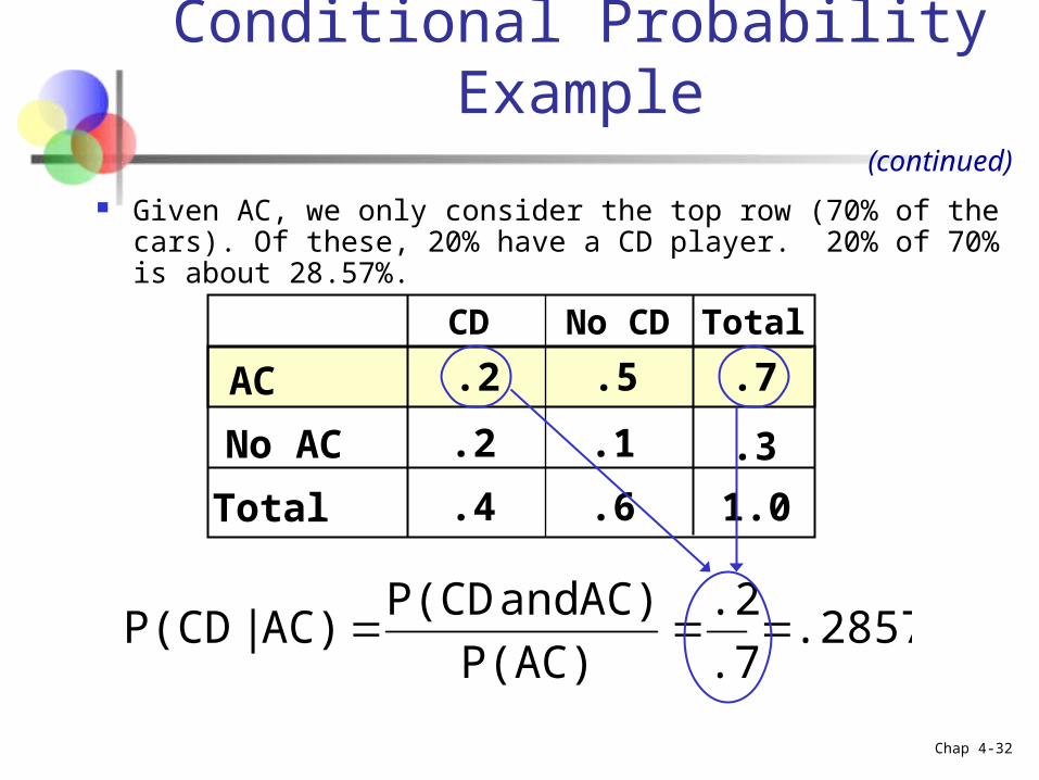
No CDCD Total
AC .2 .5 .7
No AC .2 .1 .3
Total .4 .6 1.0
Given AC, we only consider the top row (70% of the cars). Of these, 20% have a CD player. 20% of 70% is about 28.57%.
.2857.7
.2
P(AC)
AC)andP(CDAC)|P(CD
(continued)
Chap 4-33
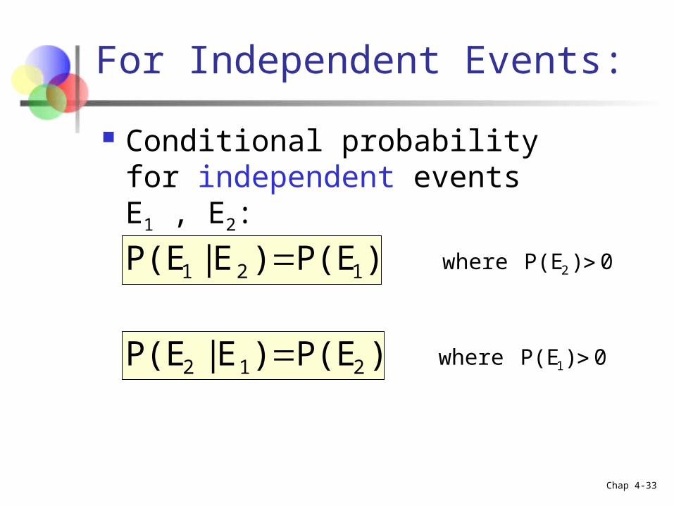
For Independent Events:
Conditional probability for independent events E1 , E2:
)P(E)E|P(E 121 0)P(Ewhere 2
)P(E)E|P(E 212 0)P(Ewhere 1
Chap 4-34
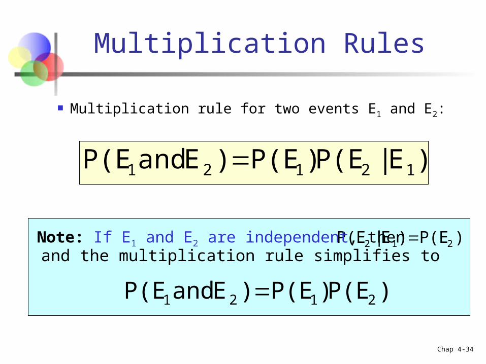
Multiplication Rules
Multiplication rule for two events E1 and E2:
)E|P(E)P(E)EandP(E 12121
)P(E)E|P(E 212 Note: If E1 and E2 are independent, thenand the multiplication rule simplifies to
)P(E)P(E)EandP(E 2121
Chap 4-35
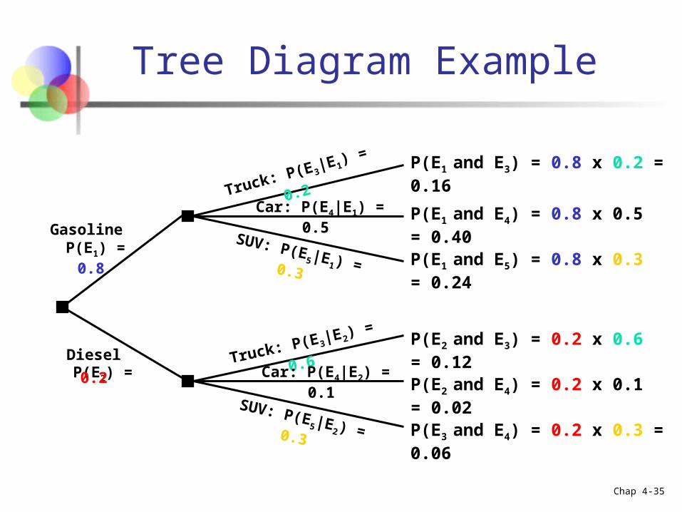
Tree Diagram Example
Diesel P(E2) = 0.2
Gasoline P(E1) = 0.8
Truck: P(E3|E1
) = 0.2
Car: P(E4|E1) = 0.5
SUV: P(E5|E1) = 0.3
P(E1 and E3) = 0.8 x 0.2 = 0.16
P(E1 and E4) = 0.8 x 0.5 = 0.40
P(E1 and E5) = 0.8 x 0.3 = 0.24
P(E2 and E3) = 0.2 x 0.6 = 0.12
P(E2 and E4) = 0.2 x 0.1 = 0.02
P(E3 and E4) = 0.2 x 0.3 = 0.06
Truck: P(E3|E2) = 0.6
Car: P(E4|E2) = 0.1
SUV: P(E5|E2) = 0.3
Chap 4-36
Get Ready….
More Probability Examples
Random Variables
Probability Distributions
Chap 4-37
Introduction to Probability Distributions
Random Variable – “X” Is a function from the sample space to
another space, usually Real line Represents a possible numerical value from
a random event Each r.v. has a Distribution Function – FX(x),
fX(x) based on that in the sample space Assigns probability to the (numerical)
outcomes (discrete values or intervals)
Chap 4-38
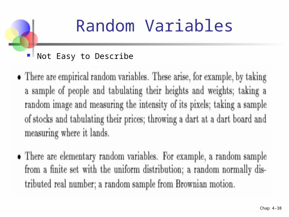
Random Variables
Not Easy to Describe
Chap 4-39
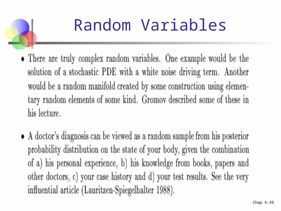
Random Variables
Chap 4-40
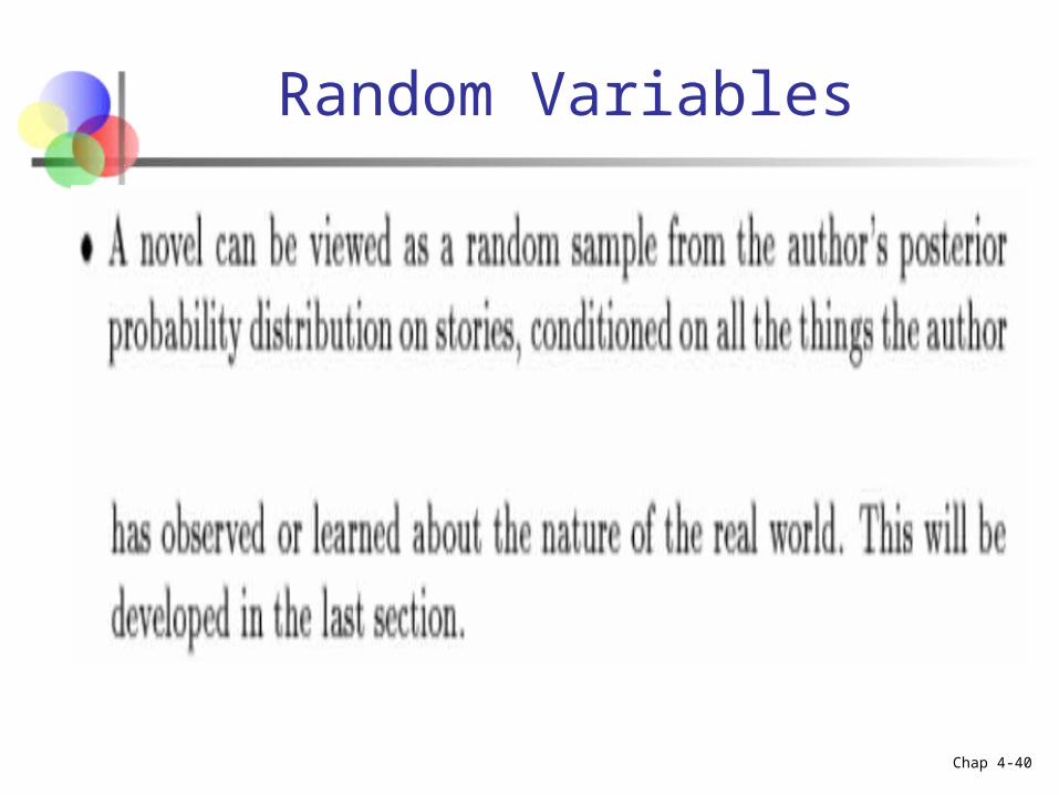
Random Variables
Not Easy to Describe
Chap 4-41
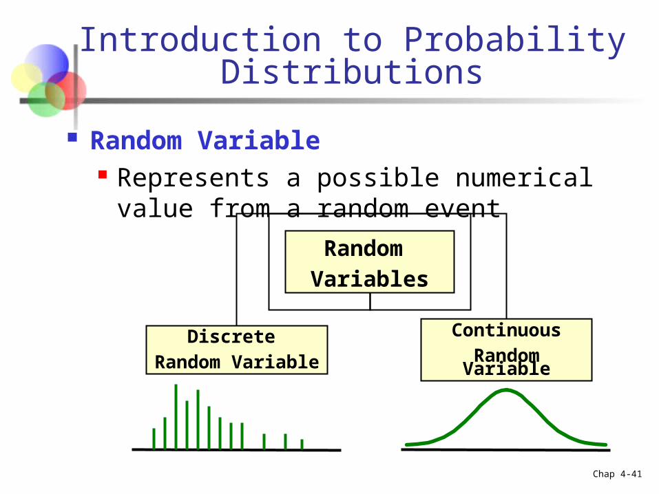
Introduction to Probability Distributions
Random Variable Represents a possible numerical value from
a random event
Random
Variables
Discrete Random Variable
ContinuousRandom Variable
Chap 4-42
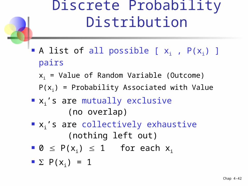
A list of all possible [ xi , P(xi) ] pairs
xi = Value of Random Variable (Outcome)
P(xi) = Probability Associated with Value
xi’s are mutually exclusive (no overlap)
xi’s are collectively exhaustive (nothing left out)
0 P(xi) 1 for each xi
P(xi) = 1
Discrete Probability Distribution
Chap 4-43
Discrete Random Variables
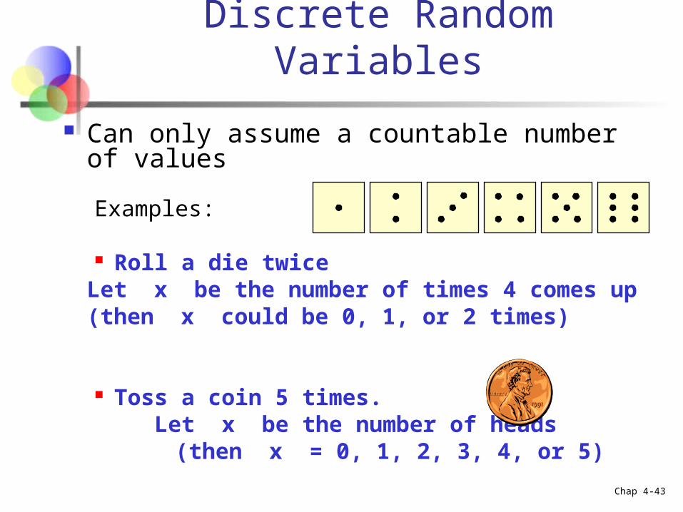
Can only assume a countable number of values
Examples:
Roll a die twiceLet x be the number of times 4 comes up (then x could be 0, 1, or 2 times)
Toss a coin 5 times. Let x be the number of heads
(then x = 0, 1, 2, 3, 4, or 5)
Chap 4-44
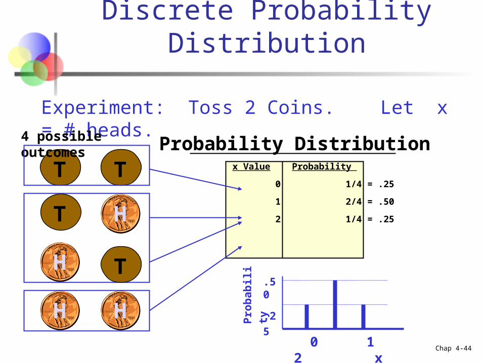
Experiment: Toss 2 Coins. Let x = # heads.
T
T
Discrete Probability Distribution
4 possible outcomes
T
T
H
H
H H
Probability Distribution
0 1 2 x
x Value Probability
0 1/4 = .25
1 2/4 = .50
2 1/4 = .25
.50
.25
Pro
bab
ility
Chap 4-45
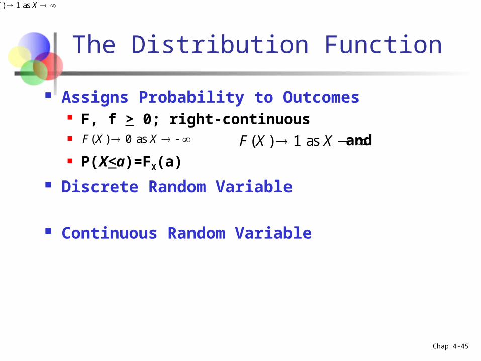
The Distribution Function
Assigns Probability to Outcomes F, f > 0; right-continuous and P(X<a)=FX(a)
Discrete Random Variable
Continuous Random Variable
( ) 0 asF X X
( ) 0 as
( ) 1 as
F X X
F X X
( ) 1 asF X X
Chap 4-46
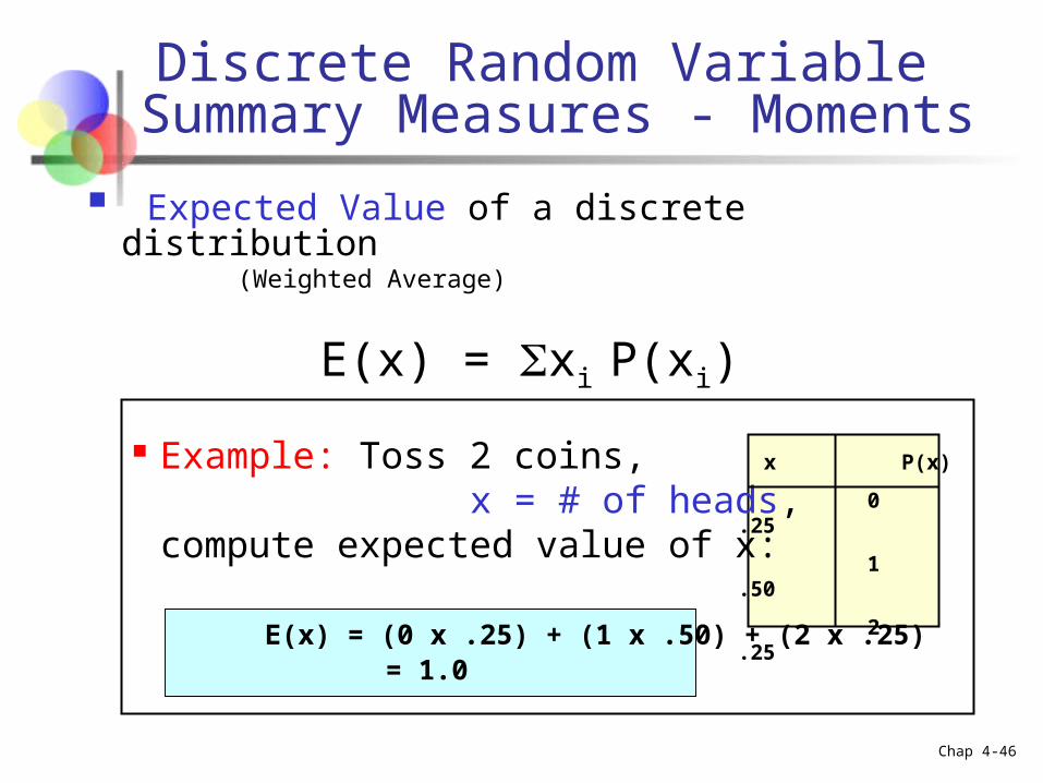
Discrete Random Variable Summary Measures - Moments
Expected Value of a discrete distribution (Weighted Average)
E(x) = xi P(xi)
Example: Toss 2 coins, x = # of heads, compute expected value of x:
E(x) = (0 x .25) + (1 x .50) + (2 x .25) = 1.0
x P(x)
0 .25
1 .50
2 .25
Chap 4-47
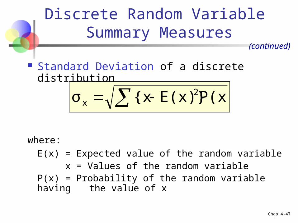
Standard Deviation of a discrete distribution
where:
E(x) = Expected value of the random variable x = Values of the random variableP(x) = Probability of the random variable having
the value of x
Discrete Random Variable Summary Measures
P(x)E(x)}{xσ 2x
(continued)
Chap 4-48
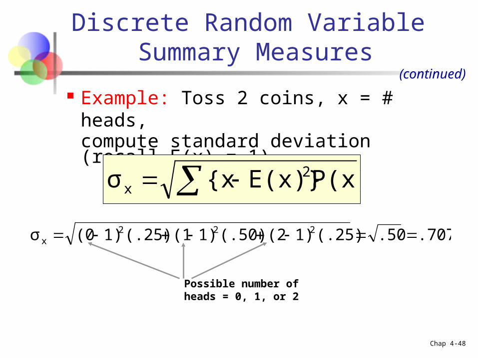
Example: Toss 2 coins, x = # heads, compute standard deviation (recall E(x) = 1)
Discrete Random Variable Summary Measures
P(x)E(x)}{xσ 2x
.707.50(.25)1)(2(.50)1)(1(.25)1)(0σ 222x
(continued)
Possible number of heads = 0, 1, or 2
Chap 4-49
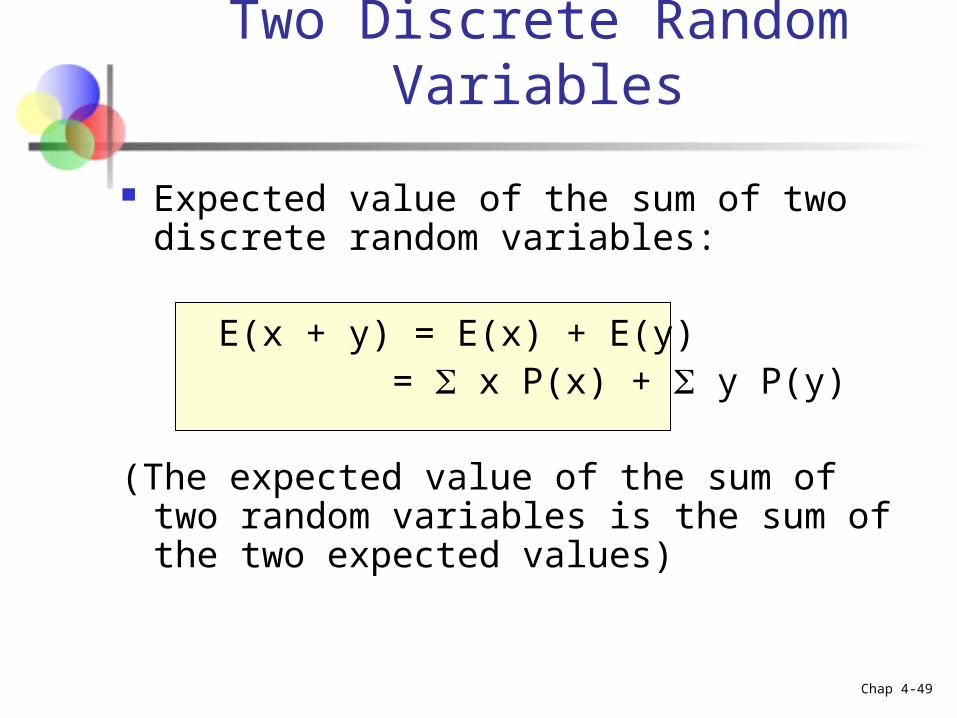
Two Discrete Random Variables
Expected value of the sum of two discrete random variables:
E(x + y) = E(x) + E(y) = x P(x) + y P(y)
(The expected value of the sum of two random variables is the sum of the two expected values)
Chap 4-50
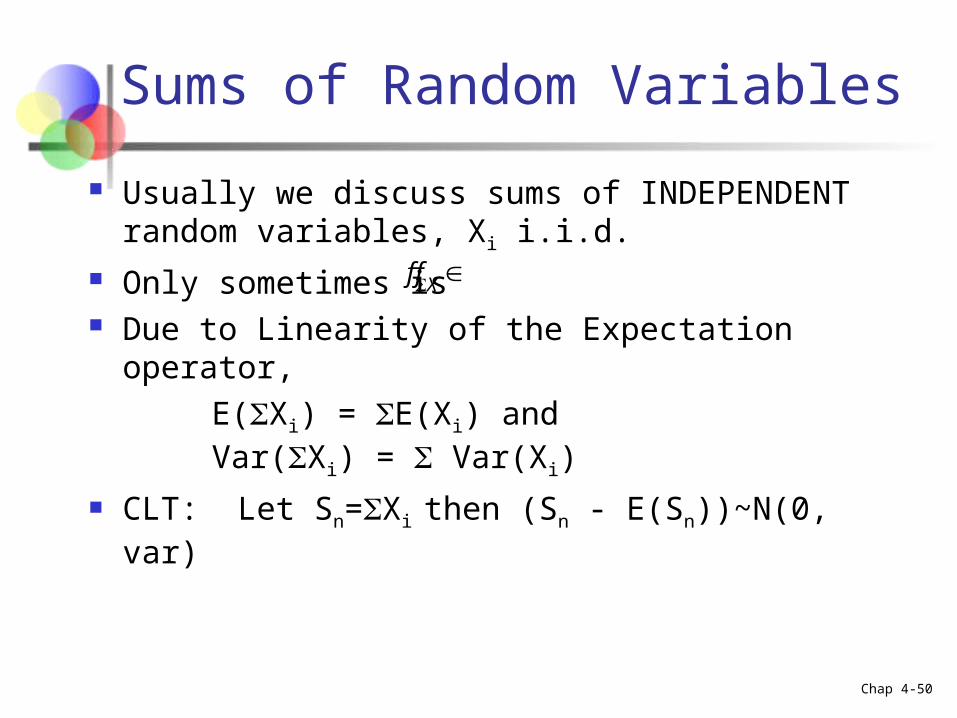
Sums of Random Variables
Usually we discuss sums of INDEPENDENT random variables, Xi i.i.d.
Only sometimes is Due to Linearity of the Expectation operator,
E(Xi) = E(Xi) and Var(Xi) = Var(Xi)
CLT: Let Sn=Xi then (Sn - E(Sn))~N(0, var)
Xf f
Chap 4-51
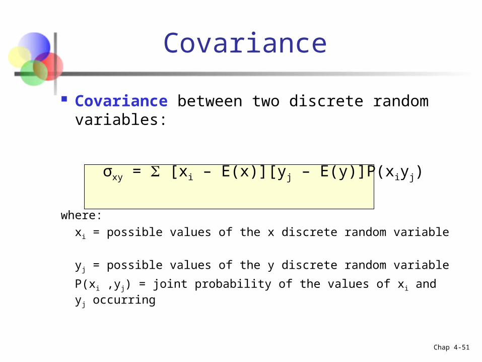
Covariance
Covariance between two discrete random variables:
σxy = [xi – E(x)][yj – E(y)]P(xiyj)
where:
xi = possible values of the x discrete random variable
yj = possible values of the y discrete random variable
P(xi ,yj) = joint probability of the values of xi and yj occurring
Chap 4-52
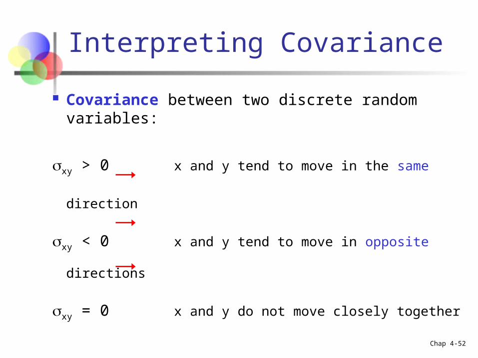
Covariance between two discrete random variables:
xy > 0 x and y tend to move in the same direction
xy < 0 x and y tend to move in opposite directions
xy = 0 x and y do not move closely together
Interpreting Covariance
Chap 4-53
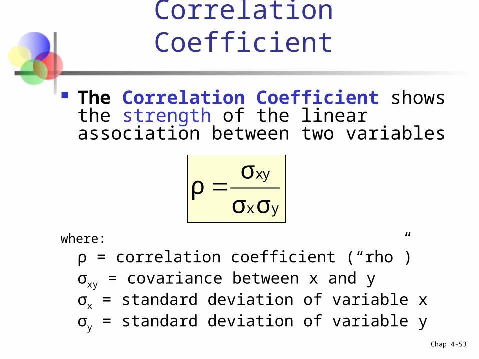
Correlation Coefficient
The Correlation Coefficient shows the strength of the linear association between two variables
where:
ρ = correlation coefficient (“rho”)σxy = covariance between x and yσx = standard deviation of variable xσy = standard deviation of variable y
yx
yx
σσ
σρ
Chap 4-54
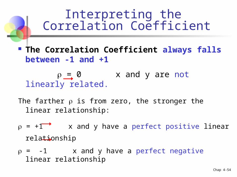
The Correlation Coefficient always falls between -1 and +1
= 0 x and y are not linearly related.
The farther is from zero, the stronger the linear relationship:
= +1 x and y have a perfect positive linear relationship
= -1 x and y have a perfect negative linear relationship
Interpreting the Correlation Coefficient
Chap 4-55
Useful Discrete Distributions
Discrete Uniform
Binary – Success/Fail (Bernoulli)
Binomial
Poisson
Empirical Piano Keys Other “stuff that happens” in life
Chap 4-56
Useful Continuous Distributions
Finite Support Uniform fX(x)=c Beta
Infinite Support Gaussian (Normal) N() Log-normal Gamma Exponential
Chap 4-57
Section Summary
Described approaches to assessing probabilities
Developed common rules of probability
Distinguished between discrete and continuous probability distributions
Examined discrete and continuous probability distributions and their moments (summary measures)
Chap 4-58
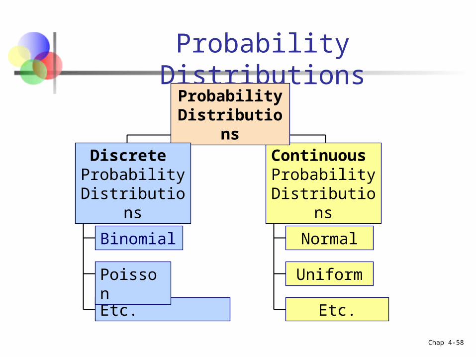
Probability Distributions
Continuous Probability
Distributions
Binomial
Etc.
Poisson
Probability Distributions
Discrete Probability
Distributions
Normal
Uniform
Etc.
Chap 4-59
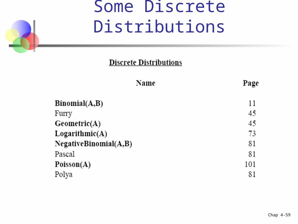
Some Discrete Distributions
Chap 4-60
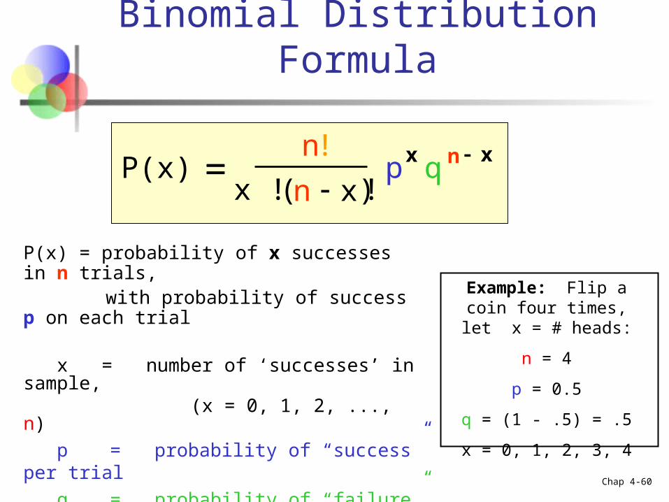
P(x) = probability of x successes in n trials, with probability of success p on each trial
x = number of ‘successes’ in sample, (x = 0, 1, 2, ..., n)
p = probability of “success” per trial
q = probability of “failure” = (1 – p)
n = number of trials (sample size)
P(x)n
x ! n xp qx n x!
( )!
Example: Flip a coin four times, let x = # heads:
n = 4
p = 0.5
q = (1 - .5) = .5
x = 0, 1, 2, 3, 4
Binomial Distribution Formula
Chap 4-61
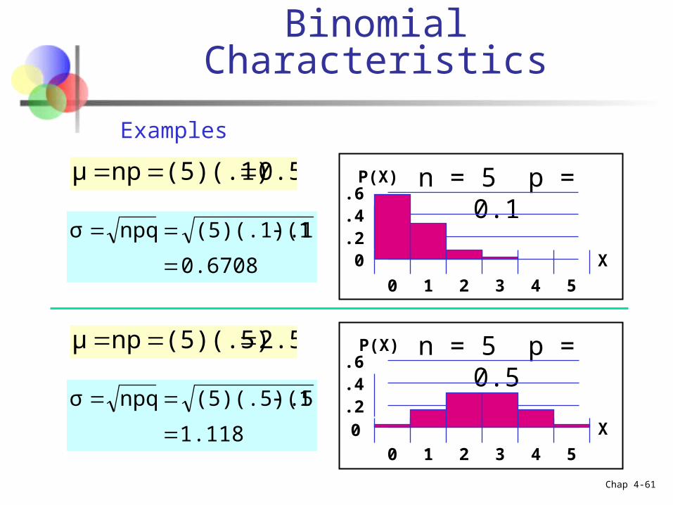
n = 5 p = 0.1
n = 5 p = 0.5
Mean
0.2.4.6
0 1 2 3 4 5
X
P(X)
.2
.4
.6
0 1 2 3 4 5
X
P(X)
0
0.5(5)(.1)npμ
0.6708
.1)(5)(.1)(1npqσ
2.5(5)(.5)npμ
1.118
.5)(5)(.5)(1npqσ
Binomial Characteristics
Examples
Chap 4-62
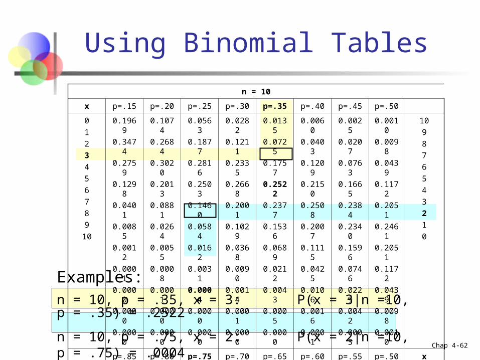
Using Binomial Tables
n = 10
x p=.15 p=.20 p=.25 p=.30 p=.35 p=.40 p=.45 p=.50
0
1
2
3
4
5
6
7
8
9
10
0.1969
0.3474
0.2759
0.1298
0.0401
0.0085
0.0012
0.0001
0.0000
0.0000
0.0000
0.1074
0.2684
0.3020
0.2013
0.0881
0.0264
0.0055
0.0008
0.0001
0.0000
0.0000
0.0563
0.1877
0.2816
0.2503
0.1460
0.0584
0.0162
0.0031
0.0004
0.0000
0.0000
0.0282
0.1211
0.2335
0.2668
0.2001
0.1029
0.0368
0.0090
0.0014
0.0001
0.0000
0.0135
0.0725
0.1757
0.2522
0.2377
0.1536
0.0689
0.0212
0.0043
0.0005
0.0000
0.0060
0.0403
0.1209
0.2150
0.2508
0.2007
0.1115
0.0425
0.0106
0.0016
0.0001
0.0025
0.0207
0.0763
0.1665
0.2384
0.2340
0.1596
0.0746
0.0229
0.0042
0.0003
0.0010
0.0098
0.0439
0.1172
0.2051
0.2461
0.2051
0.1172
0.0439
0.0098
0.0010
10
9
8
7
6
5
4
3
2
1
0
p=.85 p=.80 p=.75 p=.70 p=.65 p=.60 p=.55 p=.50 x
Examples: n = 10, p = .35, x = 3: P(x = 3|n =10, p = .35) = .2522
n = 10, p = .75, x = 2: P(x = 2|n =10, p = .75) = .0004
Chap 4-63
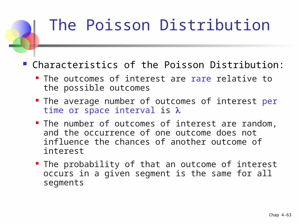
The Poisson Distribution
Characteristics of the Poisson Distribution: The outcomes of interest are rare relative to the
possible outcomes The average number of outcomes of interest per time
or space interval is The number of outcomes of interest are random, and
the occurrence of one outcome does not influence the chances of another outcome of interest
The probability of that an outcome of interest occurs in a given segment is the same for all segments
Chap 4-64
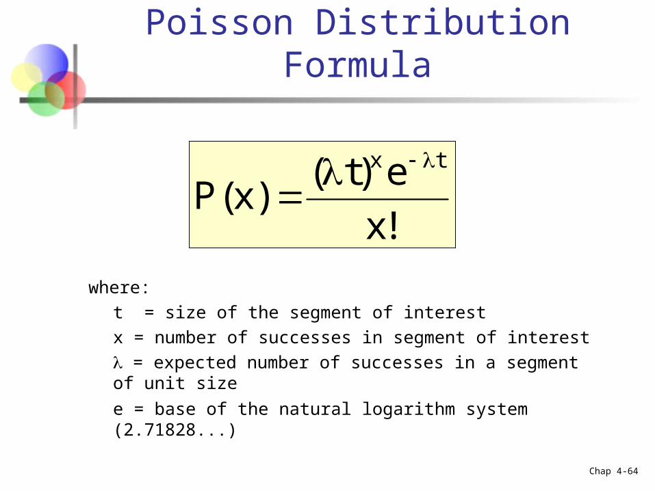
Poisson Distribution Formula
where:
t = size of the segment of interest
x = number of successes in segment of interest
= expected number of successes in a segment of unit size
e = base of the natural logarithm system (2.71828...)
!x
e)t()x(P
tx
Chap 4-65
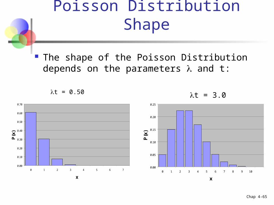
Poisson Distribution Shape
The shape of the Poisson Distribution depends on the parameters and t:
0.00
0.05
0.10
0.15
0.20
0.25
0 1 2 3 4 5 6 7 8 9 10
x
P(x
)
0.00
0.10
0.20
0.30
0.40
0.50
0.60
0.70
0 1 2 3 4 5 6 7
x
P(x
)
t = 0.50 t = 3.0
Chap 4-66
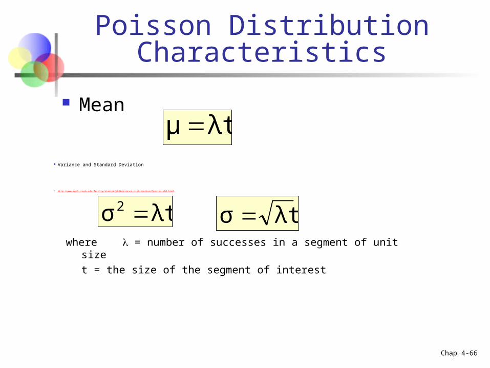
Poisson Distribution Characteristics
Mean
Variance and Standard Deviation
http://www.math.csusb.edu/faculty/stanton/m262/poisson_distribution/Poisson_old.html
λtμ
λtσ2 λtσ where = number of successes in a segment of unit size
t = the size of the segment of interest
Chap 4-67
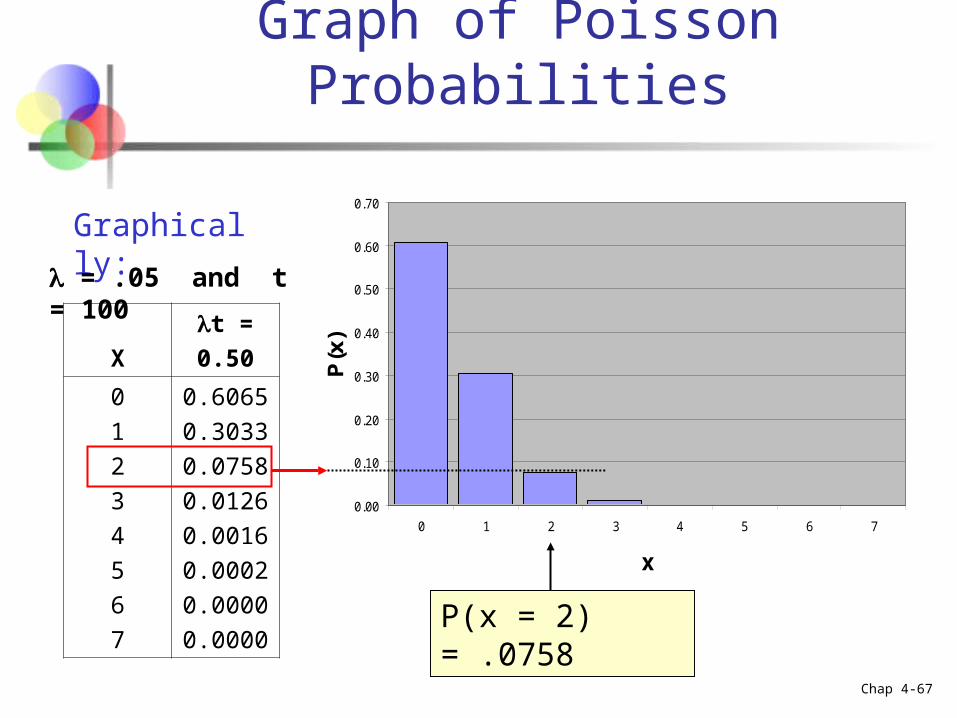
Graph of Poisson Probabilities
0.00
0.10
0.20
0.30
0.40
0.50
0.60
0.70
0 1 2 3 4 5 6 7
x
P(x
)X
t =
0.50
0
1
2
3
4
5
6
7
0.6065
0.3033
0.0758
0.0126
0.0016
0.0002
0.0000
0.0000P(x = 2) = .0758
Graphically:
= .05 and t = 100
Chap 4-68
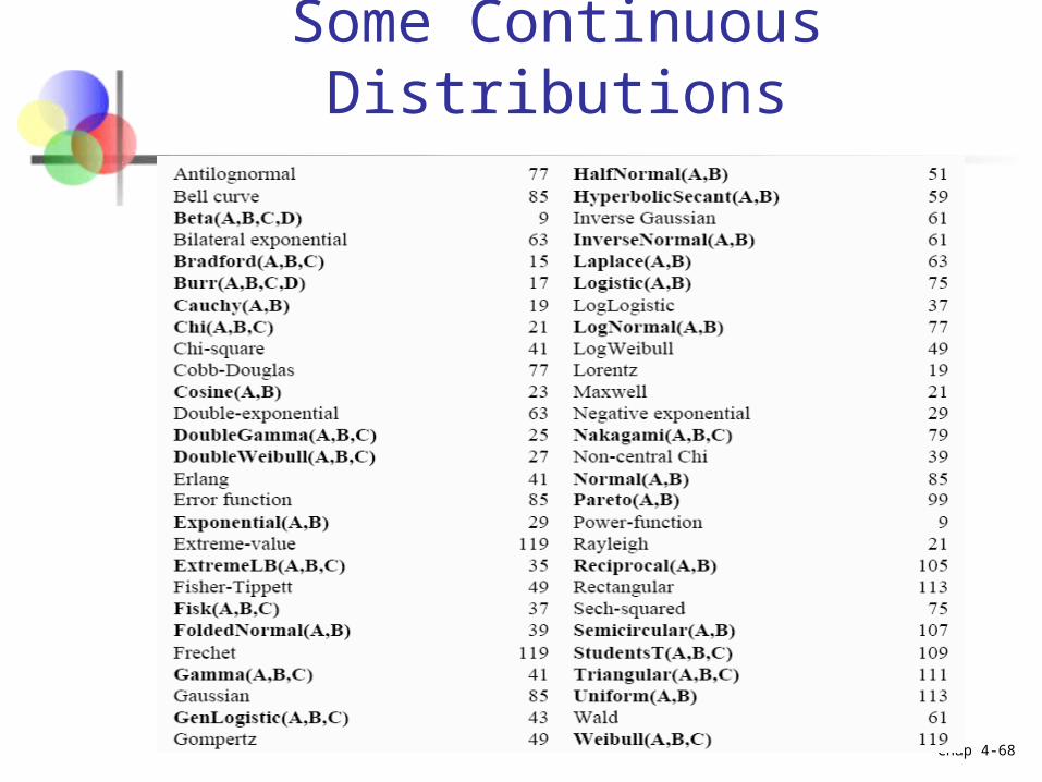
Some Continuous Distributions
Chap 4-69
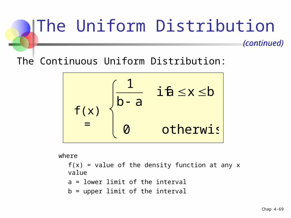
The Continuous Uniform Distribution:
otherwise 0
bxaifab
1
where
f(x) = value of the density function at any x value
a = lower limit of the interval
b = upper limit of the interval
The Uniform Distribution(continued)
f(x) =
Chap 4-70
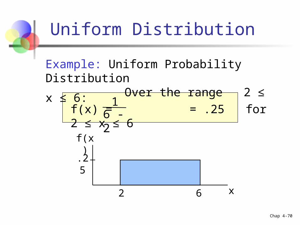
Uniform Distribution
Example: Uniform Probability Distribution Over the range 2 ≤ x ≤ 6:
2 6
.25
f(x) = = .25 for 2 ≤ x ≤ 66 - 21
x
f(x)
Chap 4-71
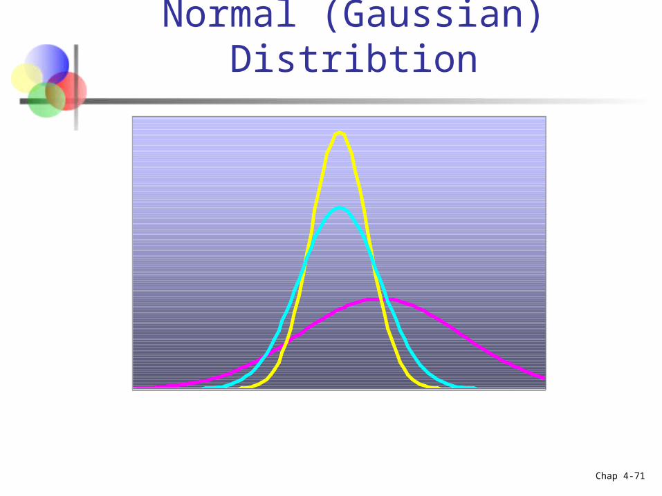
Normal (Gaussian) Distribtion
Chap 4-72
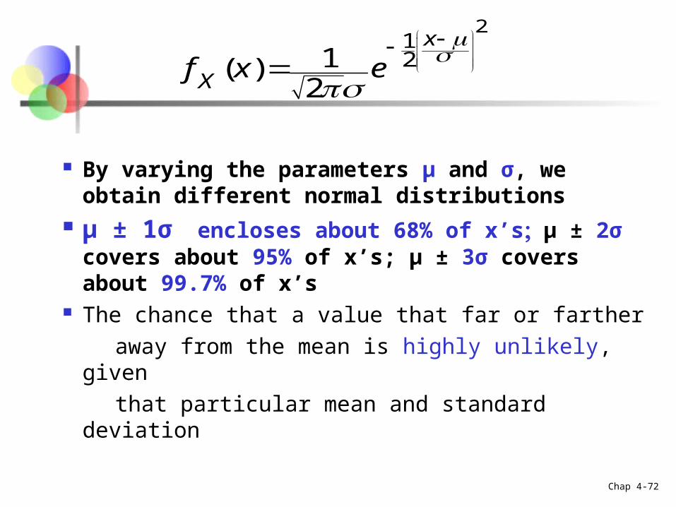
2121( )
2
x
Xf x e
By varying the parameters μ and σ, we obtain different normal distributions
μ ± 1σencloses about 68% of x’sμ ± 2σ covers about 95% of x’s; μ ± 3σ covers about 99.7% of x’s
The chance that a value that far or farther
away from the mean is highly unlikely, given
that particular mean and standard deviation
Chap 4-73
f(x)
xμ
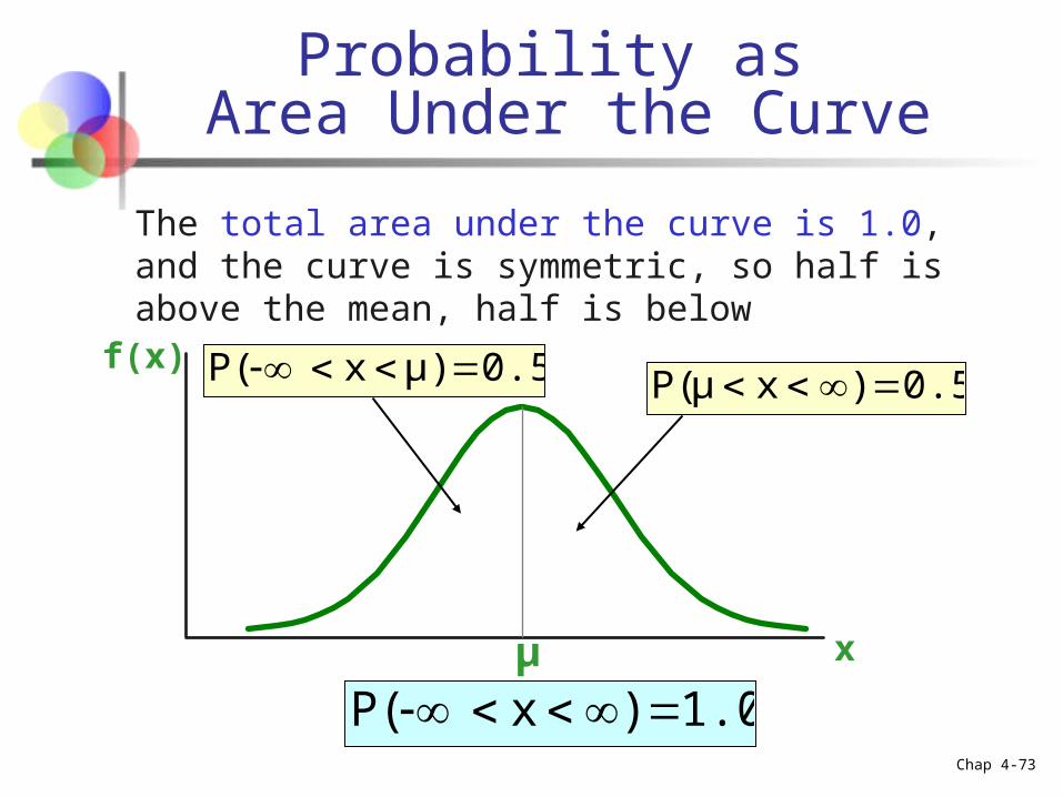
Probability as Area Under the Curve
0.50.5
The total area under the curve is 1.0, and the curve is symmetric, so half is above the mean, half is below
1.0)xP(
0.5)xP(μ 0.5μ)xP(
Chap 4-74
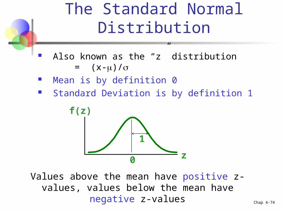
The Standard Normal Distribution
Also known as the “z” distribution = (x-)/
Mean is by definition 0 Standard Deviation is by definition 1
z
f(z)
0
1
Values above the mean have positive z-values, values below the mean have negative z-values
Chap 4-75
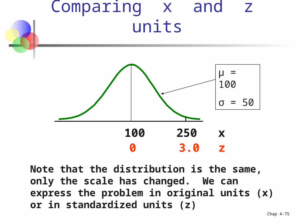
Comparing x and z units
z100
3.00250 x
Note that the distribution is the same, only the scale has changed. We can express the problem in original units (x) or in standardized units (z)
μ = 100
σ = 50
Chap 4-76
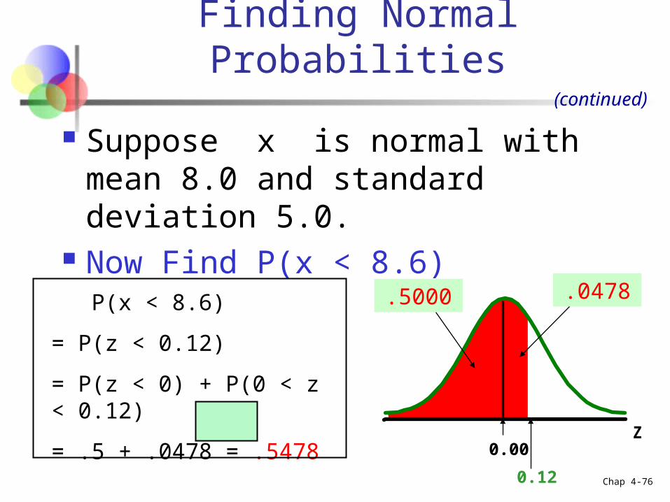
Finding Normal Probabilities
Suppose x is normal with mean 8.0 and standard deviation 5.0.
Now Find P(x < 8.6)
(continued)
Z
0.12
.0478
0.00
.5000 P(x < 8.6)
= P(z < 0.12)
= P(z < 0) + P(0 < z < 0.12)
= .5 + .0478 = .5478
Chap 4-77
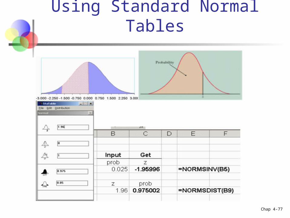
Using Standard Normal Tables
Chap 4-78
Section Summary
Reviewed discrete distributions binomial, poisson, etc.
Reviewed some continuous distributions normal, uniform, exponential
Found probabilities using formulas and tables
Recognized when to apply different distributions
Applied distributions to decision problems


![2. REVIEW of PROBABILITY AND STATISTICS (CHAP 2 - 3) [1] …miniahn/ecn425/cn2.pdf · 2007. 8. 22. · Review-1 2. REVIEW of PROBABILITY AND STATISTICS (CHAP 2 - 3) [1] Important](https://img.pdfslide.us/doc/110x75/5fcc9612f2d24e2eec5300ea/2-review-of-probability-and-statistics-chap-2-3-1-miniahnecn425cn2pdf.jpg)