Embed Size (px)
Citation preview

A GEOLOGICAL AND SEDIMETOLOGICAL APPROACK TO INFER PALEOCLIMATE FROM BURIED SOILS PROFILES WITHIN PLAYA FILLS,
SOUTHERN HIGH PLAINS, TEXAS.
by
Gabrielle Dunne BSc
A Thesis
In
Arid Land Studies
Submitted to the Graduate Faculty of Texas Tech University in
Partial Fulfillment of the Requirements for
the Degree of
Master of Science
Approved
Dr Dustin Sweet Chair of Committee
Dr Gad Perry
Dr Anthony Parsons
Dominick Casadonte Interim Dean of the Graduate School
May, 2013

Copyright 2013, Gabrielle Dunne

Texas Tech University, Gabrielle Dunne, May 2013
ii
Acknowledgments
I am very grateful to Dr. Dustin Sweet, my thesis advisor, for his advice and
guidance throughout this program. I would like to express my gratitude to Dr.
Melanie Barnes for her help and instruction in the geochemistry lab. I would
like to give my deepest appreciation to Dr. Wayne Hudnall, who gave up his
precious time to assist me in the field and allowing me to use his coring
equipment. I would also like to thank Andrew Whitesides and Juske Horita for
their assistance in the field. I acknowledge Dr. Gad Perry and Dr. Anthony
Parsons for their input while serving in the graduate committee and finally I
thank Hollee Baird for her assistance in the preparation of samples.

Texas Tech University, Gabrielle Dunne, May 2013
iii
Table of Contents
Acknowledgements ii
List of Tables ix
List of Figures xi
Abstract xiv
1. Introduction to the Southern High Plains 1
1.1 Physical Properties of the Southern High Plains 4
1.1.1 Geological Setting and Stratigraphy 4
1.1.2 The Ogallala formation 7
1.1.3 The Blackwater Draw Formation, Tahoka Formation and the Randall Clay
7
1.2. Playa Wetlands 8
1.2.1 Playas 8
1.2.2 Playa Morphology 9
1.2.3 Playa Hydrology 10
1.2.4 Playa Formation 13
1.2.5 Playas as Climate Proxies 15
1.3 Climate of the Southern High Plains 15
1.3.1 The Southern High Plains in Modern times 15
1.3.2 The Southern High Plains in Pleistocene-Holocene times 19

Texas Tech University, Gabrielle Dunne, May 2013
iv
1.4 Soils 1.4.1 Modern Soil 25
1.4.2 Soil Horizons 26
1.4.3 Soil Structure 26
1.4.4 Soil and climate 31
2. Materials, Methods and Sampling
2.1 Materials and Methods 34
2.1.1 Core Samples 34
2.1.2 Site Description 34
2.1.3 Coring 41
2.2 Physical Sampling
2.2.1 Sample preparation 42
2.2.2 Grain Size 42
2.2.3 Thin Section 43
2.3. Geochemical Sampling
2.3.1 Sample Preparation 48
2.3.2 Loss on Ignition (LOI) 48
2.3.3 Fusions 49
2.3.4 ICP/ICP-MS 47
3. Results 51
3.1. Key physical properties used in assigning soil horizonation 51
3.1.1 Bailey Playa -1 57

Texas Tech University, Gabrielle Dunne, May 2013
v
3.1.2 Bailey Playa -2 60
3.1.3 Floyd Playa -1 65
3.1.4 Floyd Playa -2 69
3.2 Geochemistry 73
3.3 Major Oxides 74
3.3.1 Bailey Playa -1 74
3.3.2 Bailey Playa -2 74
3.3.3 Floyd Playa-1 83
3.3.4 Floyd Playa-2 83
3.4 Minor Elements 89
3.4.1 Bailey Playa -1 93
3.4.2 Bailey Playa -2 93
3.4.3 Floyd Playa-1 98
3.4.4 Floyd Playa-2 98
4. Weathering Profiles 103
4.1 Weathering Ratios 105
4.1.1 Barium/Strontium Ratio 105
4.1.2 Titanium / Zirconium Ratio 105
4.1.3 Aluminum/Silica Ratio 106
4.1.4 Alkalines / Titanium Ratio 107
4.1.5 Potassium + Sodium / Aluminum Ratio 107

Texas Tech University, Gabrielle Dunne, May 2013
vi
4.1.6 Summation of Bases/Aluminum Ratio 107
4.1.7 Titanium/Aluminum Ratio 108
4.1.8 Carbonates 111
4.1.9 Iron-Manganese Nodules 113
4.2 Weathering Profiles of Playa Sediments in Bailey County
and Floyd County 113
4.2.1 Bailey Playa-1 113
4.2.2 Bailey Playa -2 120
4.2.3 Floyd Playa-1 126
4.2.4 Floyd Playa-2 126
4.2.5 Other Elemental Weathering Trends
136
4.2.6 Soil Characteristics
136
4.3 Correlation and Soil Types 139
4.3.1 Bailey Playa 139
4.3.2 Floyd Playa 143
4.3.3 Playa formation considerations
147
4.4 Temporal Constraints 148
5. Climate Proxies 158
5.1 Climo-functions 158
5.1.1 Method (1) 158

Texas Tech University, Gabrielle Dunne, May 2013
vii
5.1.2 Method (2) 159
5.1.3 Method (3) 161
5.1.4 Method (4) 161
5.2 A Summary of Climate 163
6. Summary and Conclusions 168
References 170
Appendix 181

Texas Tech University, Gabrielle Dunne, May 2013
viii
List of Tables
1.1 Proposed Processes for Playa Initiation and development 13
1.2 Major Soil Horizons 27
1.3 Soil Sub Horizons 28
1.4 Ped Structures 29
1.5 Soil Orders 32
3.1 Soil Core Nomenclature 52
3.2 Major Oxides, BP-1 75
3.3 Major Oxides, BP-2 76
3.4 Major Oxides, FP-1 77
3.5 Major Oxides, FP-2 78
3.6 Minor Elements, BP-1 89
3.7 Minor Elements, BP-2 90
3.8 Minor Elements, FP-1 91
3.9 Minor Elements, FP-2 92
4.1 Molecular Weathering and Pedogenesis Ratios 104
4.2 Stages of Carbonate accumulation in soils 112
4.3 Surface Horizons 137
4.4 Subsurface Horizons 138
5.1 Quantification of Climo-functions 158
5.2 Summary of paleotemperature 160
5.3 Summary of paleoprecipitation 162

Texas Tech University, Gabrielle Dunne, May 2013
ix
5.4 Paleoprecipitation calculated using depth to Bk 163

Texas Tech University, Gabrielle Dunne, May 2013
x
List of Figures
1.1 Study Location 6
1.2 Playa Morphology 12
1.3 Precipitation Variability 18
1.4 18O curve 20
1.5 Climate summary of the last 10 ky 23
2.1 Aerial view of Bailey Playa 36
2.2 Aerial view of Floyd Playa 36
2.3 Bailey Playa Drainage Network 38
2.4 Bailey Playa 3D model 38
2.5 Floyd Playa Drainage Network 40
2.6 Floyd Playa 3D model 40
2.7 Coring 41
2.8 Thin Sections 46
2.9 Billets 47
3.1 Stratigraphic logs 54
3.2 Grain Size BP-1 56
Texas Tech University, Gabrielle Dunne, May 2013
xi
3.3 Grain Size BP-2 64
3.4 Grain Size FP-1 68
3.5 Grain Size FP-2 71
3.6 Major Oxides BP-1 80
3.7 Major Oxides BP-2 82
3.8 Major Oxides FP-1 86
3.9 Major Oxides FP-2 88
3.10 Minor Elements BP-1 95
3.11 Minor Elements BP-2 97
3.12 Minor Elements FP-1 100
3.13 Minor Elements FP-2 102
4.1 Ti/Al parent material 110
4.2 BP-1 Weathering Ratios - I 115
4.3 BP-1 Weathering Ratios - ii 119
4.4 BP-2 Weathering Ratios - I 122
4.5 BP-2 Weathering Ratios - ii 124
4.6 FP-1 Weathering Ratios - I 128

Texas Tech University, Gabrielle Dunne, May 2013
xii
4.7 FP-1 Weathering Ratios - ii 130
4.8 FP-2 Weathering Ratios - I 132
4.9 FP-2 Weathering Ratios - ii 134
4.10 Bailey Playa Correlation 142
4.11 Floyd Playa Correlation 146
4.12 Grain Size Map 151
4.13 S-N transect 153
4.14 SW-NE transect 155
5.1 Summary of climate trends 167

Texas Tech University, Gabrielle Dunne, May 2013
xiii
Abstract
The Southern High Plains (SHP) is a large plateau with ubiquitous
playas accumulating sediment with little to no erosion for the past 1.6 Ma. The
small size and ephemeral nature of playas make them sensitive to climatic
fluctuations and often record high resolution archives. To date, climatic
studies on the SHP largely pursued pedogenic, sedimentologic and/or isotopic
data sets. Here we present whole-rock geochemical climatic signatures as a
new paleoclimate proxy for future playa studies on the SHP. Many whole-rock
geochemical ratios within soil horizons are largely driven by pedogenic
processes. Moreover, whole-rock geochemical signatures are
interchangeable between many modern soils and paleosols. Four cores (up to 4.5 m deep) were recovered from two playas on the
eastern half of the SHP (Bailey County Playa) and the western margin of the
SHP (Floyd County Playa). 2-3 buried paleosols (~1-1.5 m thick) were
recognized within each core by traditional observational techniques. Each
core shows an upward progression of buried soil type from aridisol (30-40
kyBP), to inceptisol (~21 kyBP), to mollisol (~11 kyBP) representing a
decrease in aridity. Whole-rock geochemical proxies largely follow this
progression and indicate much higher CaO and salinized zones in the lower
paleosols and an increase in leached or illuviated zones in higher paleosols.

Texas Tech University, Gabrielle Dunne, May 2013
xiv
Thus, pedogenic processes observed through traditional observation methods
and geochemical data sets agree.
Using empirically derived equations that utilize whole-rock geochemical
data, precipitation and mean annual temperature increased upward in
paleosols from ~275 mm/yr to 440 mm/yr (SE ± 147 mm/yr) and from ~ 12 to
16°C (SE ±0.6°C). Modern precipitation levels range from 330-450 mm/yr and
mean annual temperature is 18.6°C. Thus, from the oldest paleosol to the
present, these data sets indicate that precipitation increased by 50-175 mm/yr
while mean annual temperature increased by ~6°C. Our age model utilizes
previous published radiocarbon dates from nearby playas and suggests
temperature has steadily increased during soil forming events for the past ~30
ky, whereas precipitation largely increased between 21ky and 11ky soil
forming episodes. These results are similar to coeval temperature and
precipitation changes estimated elsewhere on the Great Plains.

Texas Tech University, Gabrielle Dunne, May 2013
1
Chapter 1 Introduction to the Southern High Plains
Paleoclimate can be used as a frame work for predicting variability and
thresholds of future climate change. The small size and ephemeral nature of
inundation make playa wetlands highly sensitive to climatic fluctuations and
consequently playas may be able to provide a high resolution terrestrial
archive of paleoclimate (Bowen and Johnson, 2012). Holliday et al., (1996)
study playa wetlands on the Southern High Plains which are
contemporaneous with the Blackwater Draw Formation. The multiple buried
soil profiles observed in these playas may extend back 1.6 million years,
giving them the potential to be utilized as quaternary climate proxies.
Previous studies that use playa lake sediments as a paleoclimate proxy
(Bowen and Johnson, 2012, Holliday et al., 2008, Holliday et al., 1996) focus
on carbon dating, stratigraphy and analysis of soil profiles.
Paleosols preserved in continental settings may be able to provide a
long term, continuous climatic record, equal in resolution to marine isotope
records (Retallack, 2007), especially under aggradational conditions.
Paleosols form at the Earth’s surface in direct contact with the atmosphere,
giving them potential as one of the most powerful tools in paleoclimate
interpretation (Sheldon and Tabor, 2009). Sheldon and Tabor (2009)
summarize whole-rock geochemistry methods to study paleosols in a range of
depositional setting. Geochemical ratios and trends observed within major
oxides and selected trace elements indicate pedogenic processes in
paleosols such as, weathering, leaching and illuviation that are largely
climatically driven (Sheldon & Tabor, 2009). Whole-rock geochemistry is

Texas Tech University, Gabrielle Dunne, May 2013
2
interchangeable between paleosols and modern soils allowing comparative
studies and inferences to be made regarding the conditions under which
paleosols formed (Dreise et al., 2005).
The aim of this study is to determine whether the well-established
geochemical methods of paleosol analysis as described by Sheldon and
Tabor (2009) can be successfully applied to the buried soil profiles of playa
wetlands, an area where this type of study has not been previously explored.
The objective is to apply these methods to data collected from playa wetlands
on the Southern High Plains to;
• Assess the degree of weathering within the buried soil profiles.
• Assess the grain size distribution within the soil profile.
• Assess the variability in buried soil profiles between the playa floor and
playa edge.
• Asses the variability in buried soil profiles between the eastern and
western margins of the Southern High Plains.
Comparisons between our finding and the findings of others working in the
same area which date their sediments e.g. Bowen and Johnson (2012,
Holliday et al., (2008) and Holliday et al., (1996) can be used to determine if
the whole-rock geochemistry of playa sediment can be used as a viable proxy
for interpreting quaternary climate on the Southern High Plains. Absolute
age control of the cores was not assessed; however, we utilize grain size
distribution data in comparison with the well-established northerly fining trend

Texas Tech University, Gabrielle Dunne, May 2013
3
observed in the Blackwater Draw Formation to assess reworking and thus, a
relatively younger age. Results indicate that buried soils grain size
distributions are inconsistent with the range expected within the Blackwater
Draw Formation, thus we infer that these paleosols were developed on
reworked Blackwater Draw Formation sediments, and thus younger than ~
40,000 years. Furthermore, C14 dates from nearby playas are used to bolster
the grain size comparison trends and suggest that the buried soils analyzed
range from ~11-20 ky.
The cores were obtained from the center and edge of two playas in
Texas, one located in Floyd County, which is on the edge of the eastern
escarpment and the other from Bailey County, which is further to the west (Fig
1.0). The cores crossed between two and three buried soil profiles. Samples
were obtained from each core at 100 mm intervals for analysis. For each
sample data on grain size, major elements (Wt %) and minor elements (PPM)
was collected. This data was plotted against depth and trends were analyzed
to infer the boundaries of the buried surfaces and different horizons within the
buried soil profiles. To determine the degree of weathering within each profile
ratios of mobile versus immobile elements were plotted against depth. The
pedogenic processes that we attribute as the cause, of the physical and
geochemical properties within our core, can be compared with modern
pedogenic processes resulting in similar characteristics to infer climatic
conditions at the time of their formation.

Texas Tech University, Gabrielle Dunne, May 2013
4
1.1 Physical Properties of the Southern High Plains 1.1.1 Geological Setting and Stratigraphy
The Southern High Plains also known as the Llano Estacado, is an
extensive semi-arid plateau spanning northwest Texas and eastern New
Mexico, covering an area of approximately 80,000 km2 (Holliday et al., 2008).
It lies south of the Canadian River and east of the Pecos River (Fig 1.1). The
Southern High Plains are approximately 400 km long (N-S) and 200 km wide
(E-W) and have an elevation ranging between 750 m – 1500 m (Lotspeich &
Everhart, 1962).
The development of the Pecos and Canadian river valleys are
attributed to the dissolution of salts and underlying Paleozoic evaporates by
groundwater, which led to subsidence and in turn controlled the position of the
river valleys (Gustavson, 1988). Moreover, uplift associated with the
formation of the Rocky Mountains created the hydraulic head which initiated
groundwater dissolution of the evaporites (Wood, 2002). This fluvial incision
has since isolated the Southern High Plains such that no hyrdrological
recharge outside of the Southern High Plains is currently underway. Thus,
the Southern High Plains can be thought of as an isolated plateau with no
fluvial source exterior to the region since isolation at around 1.6 Ma (Holliday,
1989).
The topography of the plateau is very flat and is interrupted only by
several dune fields and many small playa wetlands and their associated
Texas Tech University, Gabrielle Dunne, May 2013
5
lunettes (Holliday, 1989). The basal bedrock unit of the playa-lunette systems
is formed from sand and gravel eroded from the Rocky Mountains, this is
known as the Ogallala Formation (Bowen and Johnson, 2012). The Ogallala
Formation forms the largest aquifer in the U.S.A. and provides the primary
water supply for the semi-arid regions of Texas and New Mexico (Fryar et al.,
2001). A thick carbonate-rich zone forms a cap rock above the Ogallala
formation (Bowen and Johnson, 2012) this is overlain by the aeolian derived
sands and silts of the Blackwater Draw Formation (Holliday, 1989). Holliday
et al., (2008) observe playa fill on the Southern High Plains to be composed of
a pale olive green to gray clay which maybe calcareous, this it termed the
Tahoka Formation (Reeves, 1990). Above this lies the Randall Clay which is
a dark black/ gray mud (Holliday et al., 2008).

Texas Tech University, Gabrielle Dunne, May 2013
6
Figure 1.1: Location of the two study sites; Bailey Playa and Floyd Playa on the Southern High Plains (modified from Holliday, 1989).

Texas Tech University, Gabrielle Dunne, May 2013
7
1.1.2 The Ogallala Formation
The Ogallala Formation (Darton, 1905), averages 100m thick (Wood,
2002) and is Miocene-Pliocene age (Holliday et al., 1996). It forms a massive
piedmont alluvial plain on the eastern side of the southern Rocky Mountains
and forms the bedrock of the High Plains, from South Dakota to south–
eastern New Mexico (Reeves, 1972). The Ogallala Formation lies
unconformably above Permian, Triassic, Jurassic and Cretaceous strata and
is capped by a pedogenic calcrete which defines the three sides of the
Southern High Plains (Sabin and Holliday, 1995). The formation consists of a
series of alluvial deposits which filled incised bedrock valleys with clay, sand
and gravels derived from the Rocky Mountains (Hawley et al., 1976).
1.1.3 The Blackwater Draw Formation, Tahoka Formation and Randall Clay
The Blackwater Draw Formation termed by Reeves (1976) is formed
from Pleistocene cover sand, which directly overlay The Ogallala Formation.
The Blackwater Draw Formation forms a 25-30m thick sequence which is the
principal surficial deposit across much of the Southern High Plains (Hawley,
1976). The Blackwater Draw is characterized as an eolian deposit consisting
of fine sand, silt, and clay, which fine from south-west to north-east, a
relationship that suggests sediments were derived from the Pecos River
Valley (Holliday, 1989). The formation includes up to six well developed
buried soil horizons which indicate periods of episodic sedimentation

Texas Tech University, Gabrielle Dunne, May 2013
8
separated by times of landscape stability. The eolian deposition is inferred to
have occurred during times of prolonged aridity and the stability and
pedogenesis most probably occurred in periods of sub-humid to semi -arid
conditions (Holliday, 1989).
Two formations comprise the basin fill of playa wetlands on the
Southern High Plains. The Tahoka formation which is Wisconsin in age,
using pollen and vertebrate fossil analysis Reeve’s (1976) date the formation
between 20-14 ky BP. The Tahoka is comprised of two fill facies; sand –
gravel found at the basin margin, this is interpreted to be fluvial/deltaic
sediment (Evans & Meade, 1945). The other facies is found in the center of
the playa floor and is composed of a clay dominated lacustrine mud (Evans &
Meade, 1945). Above the Tahoka formation lays a surficial deposit - The
Randall Clays, a dark black smectite mud composed of silts and clays
(Holliday et al., 2008) these are thought to form under ponded conditions or
heavily vegetated sub-aerial conditions (Holliday et al., 2008).
1.2 Playa Wetlands
1.2.1 Playas
Playas are small, internally drained, ephemerally inundated wetlands
that are common throughout many arid and semi-arid regions across the
world (Bowen and Johnson, 2012). Playa wetlands are a prominent feature of
the Southern High Plains of Texas and New Mexico, it is estimated that there

Texas Tech University, Gabrielle Dunne, May 2013
9
are approximately 25,000 - 30,000 of these ephemeral lakes, which occur
above the present zone of saturation (Osterkamp and Wood, 1987a; Holliday
et al., 1996). The playas of the Southern High Plains lie on top of the
widespread Blackwater Draw Formation and lie locally above the Ogallala
Formation (Holliday et al., 1996). Small, isolated, eolian dunes called lunettes
often form downwind of playa basins (Holliday, 1997; Bowen and Johnson,
2012). Lunettes, first named by Hills (1940) are relatively low dune ridges
(<10m), and usually have a crescentic form. On the Southern High Plains the
material forming the lunettes is generally material derived from the deflation of
both the Blackwater Draw Formation and sediments from the associated
playa basin floor (Sabin and Holliday, 1995; Holliday, 1997). Playa-lunette
systems provide an array of vital roles such as groundwater recharge (Wood,
2002), surface water storage and nutrient cycling (Bowen and Johnson,
2012). A thick unsaturated zone which underlies much of the Southern High
Plains is a result of increased groundwater movement to the southeast as
seeps and springs from the escarpment edge (Wood & Osterkamp, 1987a).
Playa wetlands in this area do not occur beyond the escarpment edge of the
Southern High Plains (Wood 1987a).
1.2.2 Playa Morphology
Playa-Lunette systems tend to be characterized by several distinct
zones; (Figure 1.2). The playa floor, this area is intermittently inundated with

Texas Tech University, Gabrielle Dunne, May 2013
10
water and is underlain by hydric soil that is locally able to support aquatic
vegetation (Smith, 2003). The annulus is the sloping region between the rim
of the depression and the playa floor. Between the depression rim and the
lunette, there is a generally flat grass bench area. The lunette is a stratified
dune that forms downwind of the playa and is derived largely from calcareous
playa fill (Sabin and Holliday, 1995). The inter-playa is an upland, typically flat
region which is often mantled by loess and covers an expansive area (Bowen
and Johnson, 2012).
1.2.3 Playa Hydrology
Playas significantly influence the surface and groundwater hydrology of
the Southern High Plains by providing surface water drainage and major
zones of recharge to the Ogallala aquifer (Stone, 1990). Precipitation and
runoff are the primary surface processes acting on playa basins influencing
the shape of playa basins through the interplay between centripetal flow and
erosion by sheet wash, rill wash, and small streams that transport sediments
to the playa (Reeves, 1990).
Playas significantly influence the surface and groundwater hydrology of the
Great Plains by providing surface water drainage and major zones of
recharge to the Ogallala aquifer (Stone, 1990). Precipitation and runoff are the
primary surface processes acting on playa basins influencing the shape of
playa basins through the interplay between centripetal flow and erosion by

Texas Tech University, Gabrielle Dunne, May 2013
11
sheet wash, rill wash, and small streams that transport sediments to the playa
(Reeves, 1990).

Texas Tech University, Gabrielle Dunne, May 2013
12
Figu
re 1
.2: a
dapt
ed fr
om B
owen
and
John
son
(201
2) sh
ows t
he k
ey m
orph
olog
ical
feat
ures
of a
pla
ya w
etla
nd.

Texas Tech University, Gabrielle Dunne, May 2013
13
1.2.4 Playa Formation
Playa wetlands occur where water can periodically collect in
depressions of the lands surface. There is some degree of debate
surrounding the processes by which playa wetlands form; proposed
processes include, differential compaction (Johnson, 1901), wind deflation
(Reeves, 1966), piping (Reeves, 1966), animal activity (Reeves, 1966), and
collapse through dissolution (Gustavson and Finley, 1981). See Table 1.1,
adapted from Holiday et al., (1996).
Osterkamp and Wood (1987b) propose a mass transport model for
playa development and expansion where an initial depression, most likely
formed by removal of material by eolian processes, is inundated with surface
Table 1.1 Proposed Processes for Playa Initiation and development
Process References
Deflation Evans and Meade (1945), Reeves (1966), and Reeves and Parry (1969), Kaczrowski (1977)
Dissolution of underlying evaporites
Johnson (1901), Baker (1915), Patton (1935), Price (1944), Reeves (1971), Gustavson et al. (1980), Reeves and Temple (1986),Paine (1994)
Animal activity , (see Gilbert, 1895), Gould (1907), Baker (1915), Reeves (1966) Leaching of calcic soils and calcretes and deflation Judson (1950, 1953) Piping of fines, eluviation, and calcrete dissolution Wood and Osterkamp (1984), Osterkamp and Wood (1987) Differential compaction Johnson (1901)

Texas Tech University, Gabrielle Dunne, May 2013
14
run off from precipitation. Downward transport of fine grained clastic and
organic material occurs, oxidation of the organic material at depths which
forms carbonic acid when combined with groundwater, allows for rapid
dissolution of carbonates in the unsaturated zone; ultimately leading to more
subsidence.
Playas expand from the center outwards (Wood & Osterkamp, 1987a)
fine grained deposits on the playa floor lead to low permeability. Thus, the
annulus is the main zone of groundwater recharge (Wood & Osterkamp,
1987a). During periods of ponding piping of water and fine clastic material
into the unsaturated zone along with the eluviations of silts and clays by
ground water leads to further expansion of the playa (Wood & Osterkamp,
1987b). The size of a playa is a function of its catchment area, once the
supply of runoff is insufficient for further illuviation and dissolution, expansion
will cease (Wood & Osterkamp, 1987a).
Holliday et al., (1996) examined the lacustrine, eolian and alluvial fill of
multiple playas on the Southern High Plains, and proposed fluvial erosion and
deflation as the primary playa formation mechanism. Holliday et al., (1996)
observe that variations in the texture and grain size of the Blackwater Draw
Formation are a controlling factor in the size and distribution of Playas.
Coarse sandy areas form the most erodible substrates, followed by finer
clayey areas, where the clays form sand sized aggregates (Chepil & Woodruf,

Texas Tech University, Gabrielle Dunne, May 2013
15
1963). This supports the hypothesis for playa formation and maintenance by
deflation and erosion rather than dissolution and subsidence as proposed by
Wood and Osterkamp (1989a). Holliday et al., (1996) also suggest that the
dissolution of carbonate occurs as a result of the playa basin rather than
being the cause of the playa basin.
1.2.5 Playas as Climate Proxies
The small size and ephemeral nature of inundation make playas highly
sensitive to climatic fluctuations and consequently they may be able to
provide a high resolution terrestrial archive of palaeoclimate on the high plains
(Bowen and Johnson, 2012). It is possible that playa wetlands contain
sediment reaching as far back as 1.6 Ma, this period covers Marine Isotope
Stage (MIS) 3 and possibly reaches as far back as MIS 5 (Bowen and
Johnson, 2012). Playas on the Great Plains contain terminal Pleistocene and
Holocene fills. Thus they have the potential for providing clues to regional
landscape evolution and environmental changes (Holliday et al., 2008).
1.3 Climate of the Southern High Plains 1.3.1 The Southern High Plains in Modern Times
Russell (1945) describes the Great Plains as climate type BScDw, this
is characterized as dry, steppe, mesothermal (average temperature of coldest
month 0 - 18°C) climate, with occasional microthermal years (average

Texas Tech University, Gabrielle Dunne, May 2013
16
temperature of coldest month below 0°C) (Lotspeich & Everhart, 1962). The
continental setting of the Southern High Plains reduces the climate
modulating effects of the oceans resulting in greater seasonal variations. The
Southern High Plains experiences an average annual temperature range
between -9°C and 34°C, with a mean annual temperature (MAT) of 18.6°C
(High Plains Regional Climate Centre, 2009).
Temperatures on the Southern High Plains are generally high with 70 -
100 days per year experiencing conditions greater than 32°C (USGCRP,
2009). The average July temperature in Floyd County (Fig 1.1) is 26.5°C
(SRCC) average December temperature for Floyd County is 3°C (SRCC)
however temperatures do frequently drop below freezing.
Precipitation on the Southern High Plains is variable, it is lower during
the winter months, and higher during the summer. The average annual rainfall
of Lubbock is 473 mm; with 540 mm falling in May, 760 mm in June, 600 mm
in August and 650 mm in September (NOAA). The mean annual precipitation
(MAP) on the Southern High Plains ranges from 450 mm/year in the north
east to 330 mm/year in the south west (Bolen et al., 1989). 80% of total
precipitation falls between the months of May to October; during the winter
cold air masses from Polar Regions move south, blocking moister air masses
from the Gulf of Mexico (Llano Estacado Regional Water Plan, 2010).
Precipitation is highest during spring due to the frontal lifting of warm air

Texas Tech University, Gabrielle Dunne, May 2013
17
masses (Johnson, 2007a). During the summer months droughts often occur
as subsiding air leads to high pressure over the region, summer precipitation
tends to occur during intense convectional storms (Johnson, 2007a). Figure
1.3 shows the inter-annual variability of rainfall on the Great Plains.

Texas Tech University, Gabrielle Dunne, May 2013
18
Figu
re 1
.3: a
dapt
ed fr
om W
este
r (20
07) u
ses N
OA
A d
ata
colle
cted
from
Lub
bock
, Tex
as to
dem
onst
rate
the
inte
r-an
nual
var
iabi
lity
in ra
infa
ll on
the
Hig
h Pl
ains

Texas Tech University, Gabrielle Dunne, May 2013
19
Winds blow almost continuously across the Great Plains with gust
commonly exceeding 95 km/h (Lotspeich & Everhart, 1962). Winds speeds
tend to be greater in the early spring and autumn, with average wind velocities
in March being 50% greater than those in August (Lotspeich & Everhart,
1962). These increased wind velocities in spring and autumn often generate
localized dust storms (LERWP, 2012).
Modern Vegetation on the Great Plains is short grass prairie,
dominated by Blue Grama (Bouteloua gracilis), Buffalo Grass (Buchlöe
dactyloides) and Honey Mesquite (Prosopis glandulosa) (Johnson, 2007a).
Sand Sagebrush and Yucca are also common, while more aquatic species
such as Curltop Smartweed are able to colonies playas which are frequently
inundated after rainfall (LERWP, 2010).
1.3.2 The Southern High Plains in Pleistocene – Holocene times
During Marine Isotope Stage (MIS) 2-4 (Fig 1.4) The Laurentide ice
sheet extended across much of North America, this was known as the
Wisconsin Glaciation. At 18 ky, during MIS 2, conditions reached the Last
Glacial Maximum (LGM). During this time tundra and boreal forest extended
hundreds of miles south of the ice sheet and temperate forest retreated as far
south as Texas (Wilkins, 1991). MIS 1, 11ky ago, saw the end of the Younger

Texas Tech University, Gabrielle Dunne, May 2013
20
Figure 1.4: adapted from Porter (1989) shows the shifts in 18O
isotopes from benthic foraminifera. The peak in oxygen isotopes at
MIS2 (18,000 years ago) corresponds with the LGM. MIS stages 2-
4 correspond with the Wisconsin Glaciation.

Texas Tech University, Gabrielle Dunne, May 2013
21
Dryas and transition from the Pleistocene to the Holocene, this was
accompanied by increasing temperatures (Fritz, 2001).
Fritz (2001) examined lake records from several locations across North
America, including the Southern High Plains, Northern Great Basin and
Arizona. The records demonstrate that the whole of North America
experienced millennial scale fluctuations in climate linked with insolation and
shrinkage of the Laurentian ice sheet during MIS1. During the early
Holocene, 10 ky ago, lowered lake levels observed in the Pacific Northwest
and Northern Great Basin indicate increase aridity, this is linked with the
increased summer insolation leading to the intensification of the Pacific sub-
tropical high, preventing inflow of moist air from the west (Barnosky, 1987).
Van Devender et al., (1987) propose precipitation levels greater than today
but lower than the Pleistocene maximum around 9ky ago. This is likely due to
the southerly displacement of the jet stream. After 9ky, northward migration
of the jet stream led to a decrease in winter precipitation and drying of climate
(Fritz, 2001). At 5 Ky ago, a reduction in insolation lead to an increase in
moisture across North America, greater fluctuations in winter precipitation
were a result of shifting westerly storm tracks, high pressure cells and a shift
in the position of the winter jet (Stine, 1994).

Texas Tech University, Gabrielle Dunne, May 2013
22
Bowen and Johnson, 2012, Holliday et al., 2008, Holliday et al., 1996
have carried out stratigraphic analysis of soil profiles from playa basins
spanning MIS 5-1. Bowen and Johnson (2012) find that playa wetland
sediments suggest that during MIS 3 climate was similar to today, with warm
temperatures and low effective moisture. Sediments which correspond to the
extended inundation of the playa floor indicate a relatively cool climate and
are found in the stratigraphic record at depth corresponding to MIS 2 (Bowen
& Johnson (2012). Towards the end of MIS 2 (11-13 ky), Holliday et al.,
(2008) observe eolian sands at the base of several playa sequences on the
Southern High Plains, interpreted to be indicative of regional aridity.
MIS 1, 11 ky ago, saw the end of the Younger Dryas and the transition
from the Pleistocene to Holocene. At the Pleistocene-Holocene transition a
soil, dated between 11.8 and 9.4 ky is thought to coincide with a warming of
climate which continued through the Holocene (Bowen and Johnson. 2012).
Holliday (1989) observes lacustrine deposits followed by desiccation, dated
between 8.5 and 5.5 ky ago and infer peak aridity during this time. Between ~
9 to ~4 ky ago, Holliday (2008) observes a slowing in mud deposition which is
also linked to the warming of climate, this continued throughout the Holocene
period. Figure 1.5 adapted from Fritz (2001) provides a summary of climate
on the Southern High Plains over the last 10 ky.

Texas Tech University, Gabrielle Dunne, May 2013
23
Figure 1.5: adapted from Fritz (2001) is a summary of climate on
the Southern High Plains over the last 10ky based on
stratigraphic and sedimentological observations of Holliday
(1989).

Texas Tech University, Gabrielle Dunne, May 2013
24
It has been said that recent drought on the Southern High Plains such
as the 1930s “Dustbowl” (Worster, 1979) pale in insignificance when
compared to the “mega-droughts” experienced during the Holocene
(Woodhouse and Overpeck, 1998). One such drought occurred during the
Medieval Period ~AD 900-1300, when the Northern Hemisphere experienced
much higher temperatures than all but the most recent decades (Woodhouse
et al., 2010). This period of severe and persistent drought has been linked
with a peak in solar irradiance (MacDonald et al., 2008). Laird (2003)
suggests that atmospheric circulation was also different during this period,
with a change in shape and location of the jet stream causing a change in
associated storm tracks, shifting the moisture regime from wet to dry.
Graham et al. (2007) attributed medieval drought to sea surface temperature
(SST) anomalies i.e. strong cooling in the Pacific Ocean related to La Nina-
like conditions. Further research using the Community Atmospheric Model
(CAM) suggests that warm conditions in the North Atlantic may also be an
important factor influencing drought, particularly its aerial extent. It is thought
that a combination of both Pacific and Atlantic SST anomalies controlled the
longevity and severity of drought in the medieval period (Feng et al., 2008).
Regardless of the control, the concept of punctuated shifts in climate regime
for the Southern High Plains is important to keep in mind when evaluating
potential climate proxies in the stratigraphic record.

Texas Tech University, Gabrielle Dunne, May 2013
25
Grasslands have dominated the Southern High Plains since Miocene-
Pliocene times (Fox & Koch, 2003). Studies based on pollen analysis have
shown this to fluctuate between parkland and savannah and interspersed
short periods of deciduous woodland (Johnson, 2007a). Johnson (2007a)
uses pollen records associated with playa wetlands on the Southern High
Plains to reconstruct vegetation since the LGM. During the LGM, the region
was dominated by sagebrush grassland indicating a cool dry climate, this
transgresses into tall grass prairie towards the end Pleistocene typical of a
cooler humid environment (Johnson, 2007a). At the onset of the Holocene,
the grasslands were mixed prairie to Savannah this coincides with climatic
warming and increased aridity. Short grass ecosystems dominate from the
mid Holocene onwards (Johnson, 2007a).
1.4 Soils 1.4.1 Modern Soil
Climate is one of the most important factors influencing the formation of
soil, different soil types are restricted to different climate zones, each soil has
a specific climatic range, and features of such soils can be used to infer
paleoclimate (Retallack, 1990). Paleosols can be used in order to provide a
relatively detailed reconstruction of MAT, MAP, provenance and weathering
intensity (e.g. Sheldon & Tabor, 2009). Paleosols are also able to provide
information about atmospheric and soil gas composition including CO2 and O2
(Cerling, 1984). Soils record nutrient flux in and out of the soil, and may

Texas Tech University, Gabrielle Dunne, May 2013
26
reveal clues about moisture balance during pedogenesis, vegetation cover
and paleo-altitude (Sheldon and Tabor, 2009).
1.4.2 Soil Horizons
Paleosols profiles are divided into horizons according to color,
structure, root trace concentration, and translocation of authogenic minerals
(Tabor et al., 2008). The presence of a horizon indicates that soil forming
processes operated on a relatively stable substrate for a period of time
sufficient to allow for the reorganization of parent materials into zones of
accumulation and removal (Retallack, 1990). Table 1.2 adapted from Brady &
Nyle, (1984) summarizes the major horizons.
The master horizons are often divided into subcategories; a designated
lower case letter follows the horizon e.g. Bk or Bt, the sub horizons observed
in this study are summarized in Table 1.3 adapted from Brady & Nyle, (1984.)
1.4.2 Soil Structure
The structure of a soil is determined by the arrangement of soil
particles, and binding together into larger clusters called peds. Peds are
aggregates of soil which occur between roots cracks and burrows (Retallack,
1990). Peds can be classified into several different types, these are
summarized in Table 1.4 (adapted from Brady & Nyle (2008).

Texas Tech University, Gabrielle Dunne, May 2013
27
Table 1.2- Major Soil Horizons
Horizon Properties
O The O horizon is an organic layer made of wholly or partially decayed plant and animal debris. The O horizon generally occurs in undisturbed soil, since plowing mixes the organic material into the soil. In a forest, fallen leaves, branches, and other debris make up the O horizon.
A The A horizon, called topsoil by most growers, is the surface mineral layer where organic matter accumulates. Over time, this layer loses clay, iron, and other materials to leaching. This loss is called eluviation. Materials resistant to weathering, such as sand, tend to remain in the A horizon as other materials leach out. The A horizon provides the best environment for the growth of plant roots, microorganisms, and other life.
E The E horizon, the zone of greatest eluviation, is very leached of clay, chemicals, and organic matter. Because the chemicals that color soil have been leached out, the E layer is very light in color. It usually occurs in sandy forest soils in high rainfall areas.
B The B horizon, or subsoil, is often called the "zone of accumulation" where chemicals leached out of the A and E horizon accumulate. The word for this accumulation is illuviation. The B horizon has a lower organic matter content than the topsoil and often has more clay. The A, E, and B horizons together are known as the solum. This part of the profile is where most plant roots grow.
C The C horizon lacks the properties of the A and B horizons. It is the soil layer less touched by soil-forming processes and is usually the parent material of the soil.
R The R horizon is the underlying bedrock, such as limestone, sandstone, or granite.

Texas Tech University, Gabrielle Dunne, May 2013
28
Table 1.3 - Soil Sub Horizons
Suffix Properties
b Buried horizon. Such a soil layer is an old horizon buried by sedimentation or other processes.
c Concretions or hard nodules. a nodule is a hard "pocket" of a substance like gypsum in the soil.
g Strong gleying. Such a horizon is gray and mottled, the color of reduced (nonoxidized) iron, resulting from saturated conditions
h
Illuvial accumulation of organic matter. The symbol is used with the B horizon to show that complexes of humus and sesquioxides have washed into the hoizon. Includes only small quantities of sesquioxides. May show dark staining.
k Accumulation of carbonates. Indicates accumulation of calcium carbonate (lime) or other carbonates.
m
Cementation. The symbol indicates a soil horizon that has been cemented hard by carbonates, gypsum, or other material. A second suffix indicates the cementing agent, such as "k" for carbonates. This is a hardpan horizon; roots penetrate only through cracks
t Accumulation of silicate clays. Clay may have formed in horizon or moved into it by illuviation.
w Development of color or structure. The symbol indicates that a horizon has developed enough to show some color or structure but not enough to show illuvial accumulation of material.

Texas Tech University, Gabrielle Dunne, May 2013
29
Table 1.4 - Ped Structures
Spheroidal Plate-like Block-like Prism-like
Granular Crumb Angular sub-
angular Columnar Prismatic
Characteristic of subsurface A horizon, usually porous. Subject to wide and rapid changes.
Common in E horizons, but may occur in any part of the profile. Often inherited from the parent material, or caused by compaction.
Common in B horizons, particularly in humid regions, may occur in A horizon. Promote drainage, aeration and root penetration.
Usually found in B horizons. Common in arid and semi-arid regions.

Texas Tech University, Gabrielle Dunne, May 2013
30
The aggregation of soil particles allows for openings and hollows within
the soil. This is important for movement of air and water, these openings may
form interconnect networks called packing voids, a vuggy structure occurs
when air spaces are irregular, near spherical air spaces produce a vesicular
structure ( Retallack, 1990).
Loosely packed spherical peds cemented by organic matter produce a
granular structure, this is common in the A horizon. Large peds, with platy,
prismatic or blocky types dominate the B horizon. Platy structure results from
disruption of original bedding and addition of cement (Retallack, 1990).
Prismatic and blocky structures are often the result of continual wetting and
drying which causes swelling and shrinking of the peds, these peds are held
together by clays, carbonates, iron oxides and organic matter (Gardiner &
Miller, 2004).
Cutans are the modified surfaces of peds and come in various forms;
clay coatings (Argillans), Iron stained surfaces (ferrans), Iron/Aluminum oxide
coatings (sesquan) and calcite coatings (calcans) (Retallack, 1990). Cutans
may also form during digenesis, these tend to be much thicker than the thin
irregular cutans of the original soil (Retallack, 1990).
Isolated glaebules are another common feature of soil structure, they
possess a wide range of shapes and form from a similar variety of materials to
cutans, one example are the calcareous nodules commonly found in desert

Texas Tech University, Gabrielle Dunne, May 2013
31
soils (Retallack, 1990). Fe-Mg concretions may also form glaebules these are
generally associated with finer grained, clayey sediments with restricted
permeability and drainage (Stiles et al., 2001).
1.4.3 Soil and Climate
Paleosols can provide a direct means of reconstructing past climate,
soils form at the Earth's surface in direct contact with the atmospheric and
climatic conditions during the time of their formation thus they are in
equilibrium (Sheldon and Tabor, 2009). Paleosols contain many diagnostic
indicators of environment; different soil orders are formed under different
climatic regimes, and physical properties these are summarized in Table 1.5
(adapted from Brady & Nyle (2008).
Color can indicate the soil moisture regime in modern soils, gley colors,
(typically blue, green and-grey) and/or mottling indicates reduced conditions
typical of saturation 25-50% of the year. Gleyed soils form in restricted
horizons within the soil profile or where iron pans low down in the soil profile
and prevent run off. (Daniels et al., 1971). Thus, it can be inferred that
paleosols demonstrating similar features formed under conditions analogous
to those forming modern soils (Tabor et al., 2008).
Another indicator of climate is the calcium carbonate content of paleosols, the
presence of calcium carbonates in the Bk horizon is observed in sub-humid to
semi – arid environments (Tabor et al., 2008). In humid climates, calcium-

Texas Tech University, Gabrielle Dunne, May 2013
32
Table 1.5 - Soil Orders
Name Major characteristics
Alfisol Argillic, nitric or kandic horizons; high to medium base saturation.
Andisol From volcanic ejecta, dominated by allophone or Al-humic horizons
Aridisol Dry soil, ochric epipedon, sometimes argillic or nitric horizon
Entisol Little profile development, ochric epipedon common.
Gelisol Permafrost, often with cryoturbation Histosol Peat or bog; > 20% organic matter.
Inceptisol Embtyonic soils with few diagnostic features, Ochric or umbric epipedon, cambric horizon
Mollisol Mollic epipedon, high base saturation, dark soils, some with argillic or nitric horizons
Oxisol Oxic horizon, no argillic horizon, highly weathered.
Spodosol Spodic horizon commonly with Fe, Al oxides and humus accumulation.
Ultisol Argillic or kandic horizons, low base saturation
Vertisol High in swelling clays, deep cracks when soil is dry.

Texas Tech University, Gabrielle Dunne, May 2013
33
bearing minerals, which are easily weathered, are hydrolyzed and disappear
as calcium cations in the groundwater (Retallack, 1990). In semi-arid
environments, moisture is insufficient to remove calcium cations, evaporation
of soil-water at the wetting front can result in the precipitation of a low-
magnesium calcite in the subsurface (Bk) horizon i.e. calcic horizon (Brady &
Weil, 2008). Pedogenic calcrete precipitation is rarely observed in regions
which receive precipitation exceeding 70 mm per year (Royer, 1999),
therefore it can be interpreted that the presence of pedogenic calcrete
indicates a climate with low effective moisture.
In regions which experience seasonal rainfall, argillic and vertic (high
clay content) horizons are often observed within the calcisol (Tabor et al.,
2008). Argillic horizons are recognized by subsurface accumulations of illuvial
lattice layered clays, which appear as a waxy coating on ped surfaces (Mack
et al., 2003). In modern environments, argillic horizons develop under
conditions with free drainage and moderate seasonality (Tabor et al, 2008).

Texas Tech University, Gabrielle Dunne, May 2013
34
Chapter 2
Materials, Methods and Sampling
2.1 Materials and Methods 2.1.1 Core samples
Two cores were obtained from each playa, one from the center of the playa
floor and one from the edge of the playa floor so that any variation in
sediments between the playa center and playa edge may be sampled i.e.
sediments may be more clayey in the centre relative to the edge (Wood &
Osterkamp, 1987a).
2.1.2 Site description
The cores were taken from two playa wetlands; one in Floyd County on the
eastern margin of the Southern High Plains and one in Bailey County on the
western border of the State of Texas (Figure 1.1). A satellite image of Bailey
Playa denotes the locations of cores BP-1 and BP-2 (Fig 2.1). A satellite
image of Floyd Playa denotes the locations of cores FP-1 and FP-2 (Fig 2.2).
Figure 2.3 and 2.4, adapted from Netthisinghe (2008), display the watershed
and drainage network of Bailey Playa and a 3D view of Bailey Playa,
respectively. Figure 2.5 and Figure 2.6, adapted from Netthisinghe (2008),
display the watershed and drainage network of Floyd Playa and a 3D view of
Floyd Playa, respectively.

Texas Tech University, Gabrielle Dunne, May 2013
35
Figure 2.1: (top) Aerial photograph (from Google Earth) of the Bailey
County Playa. The two yellow pins show the location of core 1, near
the center and core, 2 at the playa edge.
Figure 2.2: (bottom) Aerial photograph (from Google Earth) showing
the location of the cores taken from Floyd County Playa. The yellow
pins show the location of core 1, towards the center of the playa and
core 2 on the eastern edge of the playa floor.

Texas Tech University, Gabrielle Dunne, May 2013
36
400 m
BP-1: 34° 1’ 14.80” N, 103° 1’ 4.02” W
BP-2: 34° 1’ 19.14” N, 103° 1’ 10.06” W
250 m
FP-1: 34° 5’ 43.60” N, 101° 7’ 0.60” W
FP-2: 34° 5’ 42.52” N, 101° 6’ 52.96” W

Texas Tech University, Gabrielle Dunne, May 2013
37
Figure 2.3: (top) adapted from Netthisinghe (2008), Digital Elevation
model of the Bailey Playa drainage network.
Figure 2.4: (bottom) adapted from Netthisinghe (2008) is a 3D model
of Bailey Playa.

Texas Tech University, Gabrielle Dunne, May 2013
38

Texas Tech University, Gabrielle Dunne, May 2013
39
Figure 2.5: (top) adapted from Netthisinghe (2008), Digital Elevation
model of Floyd Playa drainage network.
Figure 2.6: (bottom) adapted from Netthisinghe (2008) is a 3D model
of Floyd Playa.

Texas Tech University, Gabrielle Dunne, May 2013
40
• FP-1 • FP-2

Texas Tech University, Gabrielle Dunne, May 2013
41
2.1.3 Coring
A trailer mounted, concord hydraulic corer was used to obtain the four
cores (Fig 2.7). The depth of sampling ranged between 3 and 4.8 m, passing
through multiple buried soil horizons. The soil cores were encased in plastic
tubing, capped, labeled, marked with the way up and stored for lab analysis.
Figure 2.7 Field photograph of coring in Bailey Playa

Texas Tech University, Gabrielle Dunne, May 2013
42
2.2. Physical Sampling 2.2.1 Sample Preparation
The plastic tubing was split and the cores were laid out on the table for
analysis, important morphological features such as color, according to the
Munsel® Color Chart, changes in grain size, roots and nodules were recorded
on stratigraphic columns, each core was also photographed.
Samples of the core were taken every 100 mm, starting from the
bottom of the core working up to the top (i.e. modern surface). Two samples
were taken from each interval one for grain size analysis and one for
geochemical analysis. The grain size used approximately 1 g of material
which was stored in a glass vial and filled with Calgon® which acts as a
deflocculating agent.
The samples for geochemical analysis were weighed, oven dried at
50°C for 24 hours in order to remove pore water, and weighed again so loss of
water mass could be calculated. The samples were then ground to a fine
powder using a mortar and pestle and stored in glass vials for later
geochemical analysis.
2.2.2 Grain size
Samples were sonicated for a minimum of 20 minutes in order to
disaggregate clay flocculation, in some cases further dilution with Calgon®

Texas Tech University, Gabrielle Dunne, May 2013
43
solution was necessary. Once disaggregated, grain size distributions were
measured using a Beckmann-Coulter LS13320 laser particle analyzer. Grain
size variations throughout the cored soil profiles were analyzed. The D50
fraction, i.e. 50% of material is coarser and 50% finer than that grain diameter,
was measured this represents the mean. The D75 fraction i.e. the coarsest
75th percentile and D25 i.e. finest 25% of grains were also measured.
The D50 and D75 were plotted to gauge the variability in the coarse
fraction, useful for denoting deltaic sands. The symmetrical D25 fraction was
not shown because the variation from paleosol to paleosol was minimal.
Grain size distributions were plotted against depth to determine changes
between horizons and various sand fraction measurements were used to
analysis reworking of the Blackwater Draw Formation.
2.2.3 Thin sections and Billets
Several samples from the cores were made into thin sections and
examined under a microscope. These were used to identify Fe-Mn nodules,
carbonate nodules, grain coatings and illuviation (Fig 2.8). Billets were also
used to identify similar features (Fig 2.9). Nodules are 3D bodies which occur
in the ground mass, in the playa cores these are formed by calcite or Fe-Mn.
Calcite nodules are generally indicative of arid soils (Barchhardt &
Lienkaemper, 1999) while Fe-Mn nodules tend to form in soils subject to
intense seasonal change (Stiles, 2001). Illuviation is the re-deposition of

Texas Tech University, Gabrielle Dunne, May 2013
44
clays, organic matter and other material, mobilized by water from
precipitation, from one horizon into another which is generally lower in the soil
profile (Brady & Nyle, 2008). Clay coatings or cutans (Retallack, 1990) form
as a result of illuviation, when drier, deeper horizons are reached water is
suctioned into microvoids resulting in the deposition of clays which form a thin
coating on peds.

Texas Tech University, Gabrielle Dunne, May 2013
45
Figure 2.8: Photomicrographs showing key physical soil features in
each core. A) Taken from BP-1-125 and shown in plane light, vertical
section cutting through several carbonate nodules, some of which
display clay coatings. B) Horizontal section taken from BP2-270 in
cross polar light displays a Fe-Mn nodule with a clay coating. C)
Taken from BP-1-215 and shown in plane light, horizontal view
displaying Fe-Mn staining of the matrix. D) Viewed in plane light is a
horizontal section taken from FP-2-395 cm, photomicrograph displays
accumulations of Fe with diffused boundaries surrounding the grains.
E) Taken from BP-1-320 is a horizontal view in cross polar light, the
lighter colored area demonstrates clay illuviation with Fe-Mn staining
of the clay portion. F) Taken from FP-2-285 under plane light, vertical
view of an illuviation pipe. G) Taken from BP2-150 shows a vertical,
plane light view of clay illuviation. H) Taken from BP-1-335 cm
under cross polar light displaying cutans surrounding the grains.

Texas Tech University, Gabrielle Dunne, May 2013
46

Texas Tech University, Gabrielle Dunne, May 2013
47
Figure 2.9: Photographs of billets taken from BP-2, A) shows a
horizontal view through a calcium carbonate nodule with a diffused
margin; B) shows evidence of illuviation and clay-filled paleo-root
traces; C) is a vertical view of root traces; D) is a horizontal view
across a an illuviation pipe.

Texas Tech University, Gabrielle Dunne, May 2013
48
2.3. Geochemical Sampling 2.3.1 Sample Preparation
The samples for geochemical analysis were weighed, oven dried at
50°C for 24 hours in order to remove pore water, and weighed again so loss of
water mass could be calculated. The samples were then ground to a fine
powder using a mortar and pestle and stored in glass vials for later
geochemical analysis.
2.3.2. Loss on Ignition (LOI)
Porcelain crucibles are heated in a muffle furnace at 1000°C for 20
minutes, and left to cool in a desiccator for 15 minutes before they are
weighed and the mass is recorded. ~2 g of sample is added and the crucible
is weighed again. The sample is then heated in the muffle furnace at 1000°C
for 30 minutes, and allowed to cool in the desiccator for a further 15 minutes
before being weighed again. The LOI is the calculated using the following
equation (Eqn 1). This data can be found in Appendices 1. LOI data is used
when calculating the totals for each sample, the sum of the Wt% of each
element and the LOI should equal 100.
LOI = [(crucible + wet sample)-(crucible + dry sample)/ (1)
(crucible + wet sample) - crucible] x 100

Texas Tech University, Gabrielle Dunne, May 2013
49
2.3.3 Fusions
For each sample, 0.6000 +/- 0.0006 g of Lithium metaborate flux is
measured out in a porcelain crucible and poured into a platinum crucible.
0.2000 +/- 0.0002g of sample is then weighed in the porcelain crucible and a
further 0.6000 +/- 0.0006 g of Lithium metaborate flux is added. This is
thoroughly mixed and added to the platinum crucible. The M4 Claisse Fluxer
is then set up to run, 3 samples can be run at a time. Using a repipeter,
Teflon beakers are filled with 80 ml of 5%HNO3 and 1%HCl V/V acid. 20 µl of
Lithium Iodide are then dropped into the centre of the sample in the platinum
crucible. Each crucible containing sample is then clipped into the M4 Fluxer
and the Teflon beakers of acid are place in the tray below. Fluxer program P6
is selected and the samples are run, the samples are heated until molten and
then poured into the acid and stirred using magnets. Once the program is
finished, samples are transferred into 125 ml wide mouthed bottles and
labeled for trace element analysis. Samples for major element analysis are
diluted; 20 ml of sample are pipetted into a 125 ml wide mouth bottle
containing 40 ml of 5%HNO3 and 1%HCl V/V acid.
2.3.4 ICP/ ICP-MS
Using a Teledynen Leeman Labs Prodigy ICP (inductively coupled
plasma) the samples were analyzed for Si, Ti, Al, Mn, Mg, Fe, Ca, Na, K, P,
Sr, Ba, Zr and Y. A calibration for major elements was set up using the

Texas Tech University, Gabrielle Dunne, May 2013
50
following in house rock standards; BLANK, BHVO, BCM, MHA, RGMT and
1.5 BCM these standards have been analyzed using USGS rock standards at
five different labs using two techniques (XRF and ICP). The instrument was
recalibrated using these standards, which were run as samples, when data
drifted outside of 5% of this range. All samples fell within 5% of the highest
value for that element.
For the Minor elements, the following in house standards were used;
BLANK, BHVO, BCM, MHA, RGMT, STM, SCo and GSP. The instrument was
recalibrated when elements drifted outside of 10% of the calibration range.
We found recalibration was more efficient than drift calculations; therefore the
resulting data set is within 5% of the actual value for major elements and 10%
for minor elements, realistically most samples are within 3% for major
elements. The detection limit for this instrument is 4 ppm, elements which are
below this may fall below the lower limit of quantification, all of my values fall
above this limit.

Texas Tech University, Gabrielle Dunne, May 2013
51
Chapter 3 Results
The physical and geochemical properties of the playa cores are
presented in this section. Physical properties such as color, structures,
nodules and root traces are presented as graphic and photographic logs.
Grain size data is plotted against depth and is spatially matched with the
graphic log. The various wt% and ratios of major and minor elements within
the core are also plotted against depth and matched spatially with the graphic
logs. Thus, it is possible to infer the various soil horizons.
Figure 3.1 shows graphic and photographic logs from the four cores,
BP-1, BP-2, FP-1 and FP-2. Each core was analyzed for the presence of
buried soils using standard pedological practices, two to three distinct
intervals with different pedological characteristics were found. Table 3.1
provides a summary of the nomenclature used.
3.1 Key physical properties used in assigningsoil horizonation

Texas Tech University, Gabrielle Dunne, May 2013
52
Table 3.1 - Soil Core Nomenclature Symbol Description
Modern soil
b Buried soil * S Buried soil surface**
A A Horizon B B Horizon
C C Horizon
Lowercase suffix indicate sub-horizon***
* followed by number, beginning at 1 with the first buried horizon ** followed by number, beginning at 1 with the first buried surface *** See table 1.4

Texas Tech University, Gabrielle Dunne, May 2013
53
Figure 3.1: Photographic and stratigraphic logs for the four cores,
depth in cm is marked down the side. Colors are assigned according to
the Munssel® color chart and other key physical properties are
depicted. Buried soil surfaces are denoted S and buried soils are
denoted b.

Texas Tech University, Gabrielle Dunne, May 2013
54

Texas Tech University, Gabrielle Dunne, May 2013
55
Figure 3.2: Grain size in µm is plotted against depth in cm and matched with
the stratigraphic log. An increase in grain size corresponds with S3 and
remains increased through b2 until the Btkb2 horizon. Above S2 grain size
becomes much finer. Refer to Figure 3.1 for a key to symbols on the
stratigraphic log.

Texas Tech University, Gabrielle Dunne, May 2013
56

Texas Tech University, Gabrielle Dunne, May 2013
57
3.1.1 Bailey Playa-1
BP-1 (Fig 3.1) has three buried surfaces, S1, S2 and S3. S1 occurs at
a depth of 120 cm, S2 at 215 cm and S3 at 320cm. This section contains four
distinct intervals based on varying pedogenic characteristics. Each interval is
separately described and interpreted below. This core was found to; the
modern soils and three buried soils, b1, b2 and b3.
Modern Soil
The first horizon is dark in color, N3, due to its increased organic
content and also contains many organic woody roots. The lower horizon (20-
120 cm) contains vertically oriented pipes of finer grained material and
organics.
This horizon is interpreted to be the modern soil, the upper horizon
forms the A horizon (top soil) (Table 1.2) as indicated by abundance of
organic woody roots. The lower horizon also contains organic roots, but to a
lesser degree, and the vertical pipes of fines are indications of illuviation.
Thus, the interval is best inferred as a Bht horizon (Table 1.3).
Buried Soil 1
Interval b1 (Fig 3.1) is color 10YR4/2, at the top (120-140 cm) there is
a sub horizon containing carbonate nodules (Fig 2.9: A) this horizon

Texas Tech University, Gabrielle Dunne, May 2013
58
demonstrates vertical piping of fine grained material. Below this (150-175 cm)
is a sub horizon which is characterized by further vertical piping of fine
grained material, this horizon also contains some organic root traces. In the
deepest horizon of b1 (175-215 cm), small black concretions and organic root
traces are observed along with some vertical pipes which display a difference
in color from the surrounding material. Grain size remains relatively low
throughout b1 (Fig 3.2).
The horizonation observed throughout b1 leads to the inference of a B
horizon (Table 1.2). The piping of fines observed in the upper sub horizon is
interpreted as the illuviation of clays. The presence of clay illuviation and
carbonate nodules in this horizon are interpreted as a Btk horizon (Table 1.3).
The piping of fines in the middle horizon is again interpreted as illuviation of
clays, thus a Bt horizon is inferred (Table 1.3). The dark concretions
observed in the deepest horizon are inferred as Fe-Mn nodules. The color
variation is interpreted as development of color structure these characteristic
are best described by a Bwc horizon (Table 1.3).
Buried Soil 2
Interval b2 (Fig 3.1) is color 10YR4/2, and contains 3 sub-horizons.
The upper horizon (215-250 cm) contains black nodules and some vertical
piping of fines. In this unit a small peak is observed in the D75 portion of the
grain size (Fig 3.2). Below this (250-260 cm) a thin sub horizon occurs which

Texas Tech University, Gabrielle Dunne, May 2013
59
contains calcite nodules and further piping of fines. D75 and D50 portions of the
grain size increase in this unit (Fig 3.2). The lower unit (260-320 cm) contains
black nodules towards the top of the unit (Fig 2.8: C) and some cementation
of the grains. D75 and D50 portions of the grain size remain high at the top of
this sub horizon but decrease toward the bottom (Fig 3.2).
Horizonation within this soil leads to its interpretation as a B horizon
(Table 1.2). In the upper horizon the dark concretions are interpreted as Fe-
Mn nodules, the piping of fines is interpreted as clay illuviation, thus a Btc
horizon best fits this soil (Table 1.3). In the middle horizon the piping of fines
is interpreted as the illuviation of clays. The presence of clay illuviation and
carbonate nodules in this horizon are interpreted as a Btk horizon (Table 1.3).
In the deepest horizon the dark concretions are interpreted as Fe-Mn nodules,
the presence of concretions and cementation leads to the inference of a Bmc
horizon (Table 1.3).
Buried Soil 3
Interval b3 (Fig 3.1) is color 10YR5/4, only the top portion of this unit
was retrieved in the core. This horizon demonstrates vertical piping of fines,
with black staining (Fig 2.8 E), thin coatings are also observed surrounding
the grains (Fig 2.8: H). The area of finer grained dark material is interpreted
as a clay illuviation pipe, stained by Fe-Mn, the coatings on the grains are

Texas Tech University, Gabrielle Dunne, May 2013
60
interpreted as cutans (Retallack, 1990) both of these features are indicative of
clay illuviation thus a Bt horizon is inferred (Table 1.3).
3.1.2 Bailey Playa -2
In BP-2, (Fig 3.1) three surfaces are identified; surfaces are inferred at
depths of 145 cm (S1), 215 cm (S2) and 315 cm (S3). This section contains
four distinct intervals based on varying pedogenic characteristics interpreted
to be; the modern soils and three buried soils, b1, b2 and b3.
The modern soil
The first interval contains 3 sub-horizons, it is dark in color, N3 at the top,
toward the bottom of this soil a color change to 5YR6/1 is observed. The
upper horizon of this section (0 -20 cm) contains organic root fragments. The
middle horizon (20-60 cm) displays some vertical piping of fine grained and
organic material and contains organic root fragments. In the deepest unit (60-
145 cm) root fragments display orange coatings, some areas of sediment
display blue/grey to green/grey discoloration, vertical piping of fines are also
noted.
This soil is interpreted to be the modern soil, the upper horizon forms
the A horizon (top soil) (Table 1.2) as indicated by abundance of organic
woody roots. The middle horizon also contains organic roots, but to a lesser
degree, and the vertical pipes of fines and organics are indications of

Texas Tech University, Gabrielle Dunne, May 2013
61
illuviation. Thus, the interval is best inferred as a Bht horizon (Table 1.3). In
the deepest horizon the orange discoloration of roots is interpreted as a result
of oxidation, the blue/grey to green/grey discoloration is likely the effect of
gleying and the piping of fines indicate illuviation, thus a Btg horizon is
inferred (Table 1.3).
Buried Soil 1
Interval b1 (Fig 3.1), has a color 5YR6/1 and contains two sub-
horizons. The upper sub-horizon (145-200 cm) contains dark concretions and
prominent piping of lighter colored fines (Fig 2.8: G). In the horizon below
(200-215 cm) carbonate nodules become prominent and an abrupt peak in
D75 and D50 portions of the grain size is observed (Fig 3.3).
In the upper unit, the dark nodules are identified as Fe-Mn nodules,
piping of fines is interpreted as illuviation, thus a Btc horizon is inferred (Table
1.3). The dominance of carbonates in the lower unit is interpreted as a Bk
horizon (Table 1.3).
Buried Soil 2
Interval b2 (Fig 3.1), has a color 5YR6/1 and contains two sub-horizons. The
upper unit (215-230 cm) is thin and demonstrates vertical piping of fines. The
lower unit (230-310 cm) contains black concretions (Fig 2.8: B) and carbonate

Texas Tech University, Gabrielle Dunne, May 2013
62
nodules. Grain size then increases and fluctuates between 50 µm and 100
µm throughout b2 (Fig 3.3).
In the upper unit, piping of fines is interpreted as illuviation, thus a Bt
horizon is inferred (Table 1.3). The black concretions in the lower horizon are
interpreted as Fe-Mn nodules, the presence of nodules and carbonate leads
to its classification as a Bck horizon (Table 1.3).
Buried Soil 3
Interval b3 (Fig 3.1) has a color 10YR5/4, and contains two sub-
horizons. Only the top part of this unit was retrieved in this core. The upper
unit (310-335 cm) contains black concretions and spots of orange
discoloration. The lower unit 335 cm – end of core) is dominated by calcite
nodules. At S3, an abrupt decreases in the D50 and D75 fractions is observed,
grain size remains relatively low through b3 (Fig 3.3).
In the upper unit, the black concretions are interpreted as Fe-Mn
nodules, the orange discoloration is likely due to oxidation, thus a Bc horizon
is inferred (Table 1.3) The dominance of calcite nodules in the lower horizon
leads to the inference of a Bk horizon (Table 1.3).

Texas Tech University, Gabrielle Dunne, May 2013
63
Figure 3.3: Grain size in µm is plotted against depth in cm and
matched with the stratigraphic log. A small increase in the D75 portion
corresponds with S1. A larger increase in grain size corresponds with
S2, below S3 a reduction in grain size occurs. The D75 portion
fluctuates through b1 and b2. Refer to Figure 3.1 for a key to symbols
on the stratigraphic log.

Texas Tech University, Gabrielle Dunne, May 2013
64
Texas Tech University, Gabrielle Dunne, May 2013
65
3.1.3 Floyd Playa-1
FP-1 (Fig 3.1) is largely homogenous in appearance and contains
missing data between 255 cm and 215 cm where the core was unrecovered.
There are two inferred buried surfaces one at a depth of 200 cm (S1), and
one at 310 cm (S2). There are three distinct intervals based on varying
pedogenic characteristics observed within this core, these are interpreted as;
the modern soil and two buried soils, b1 and b2. Figure 3.4 shows the grain
size data for core FP-1, the fluctuations of grain size within this core are very
small when compared with the other three cores.
The modern soil
The upper interval contains 3 sub-horizons. The upper unit (0-45 cm)
has a color 5YR2/2, and contains woody organic root structures. The horizon
below (45-165 cm) is 10YR2/2 color and demonstrates vertical piping of fines
and organic matter, woody roots are observed. The lower unit (165-200 cm)
is 5YR6/1 color and also contains woody root material and demonstrates
piping of fines. A small peak in grain size occurs just above within the modern
soil just above S1 (Fig 3.4).
This soil is interpreted to be the modern soil, the upper horizon forms
the A horizon (top soil) (Table 1.2) as indicated by abundance of organic
woody roots. The middle horizon also contains organic roots, but to a lesser
degree, and the vertical pipes of fines and organics are indications of

Texas Tech University, Gabrielle Dunne, May 2013
66
illuviation. Thus, the interval is best inferred as a Bht horizon (Table 1.3). In
the lower unit piping of fines is interpreted as illuviation of clays, thus a Bt
Horizon is inferred (Table 1.3).
Buried Soil 1
Interval b1 (200-305 cm) (Fig 3.1) is 10YR4/2 color, no sub-horizons
were observed and a section of this horizon could not be retrieved. This unit
contains black nodules towards the bottom, piping of fines is also observed.
The concretions are interpreted as Fe-Mn nodules and piping of fines
indicates illuviation, thus a Btc horizon is inferred (Table 1.3).
Buried Soil 2
Only the top of b2 (Fig 3.1) was retrieved, this unit is 10YR4/2 color, it
is dominated by carbonate nodules and contains weakly developed pipes
which display small variations in color and grain size. These variation
structures are not developed well enough to be interpreted as illuviation, thus
it is interpreted as a Bwk horizon (Table 1.3).
Texas Tech University, Gabrielle Dunne, May 2013
67
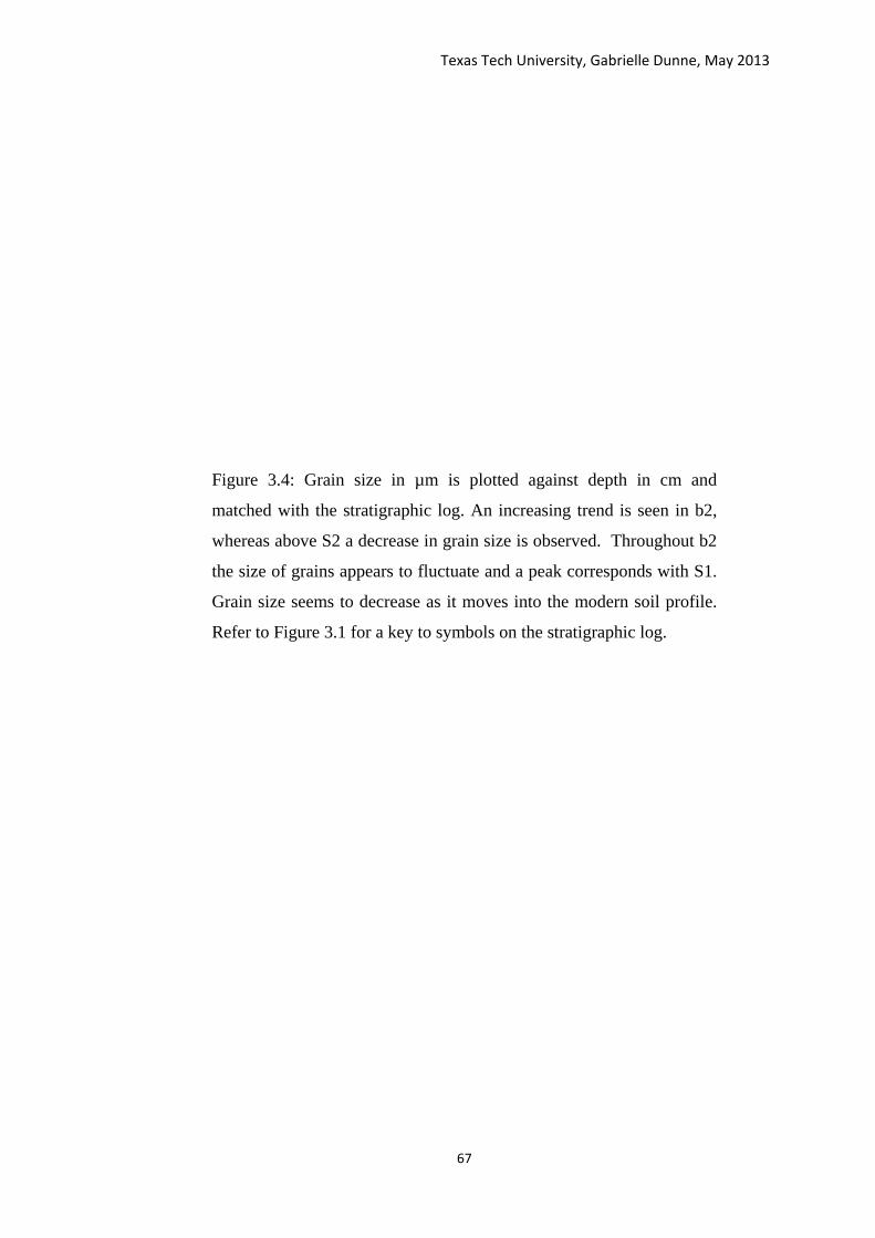
Figure 3.4: Grain size in µm is plotted against depth in cm and
matched with the stratigraphic log. An increasing trend is seen in b2,
whereas above S2 a decrease in grain size is observed. Throughout b2
the size of grains appears to fluctuate and a peak corresponds with S1.
Grain size seems to decrease as it moves into the modern soil profile.
Refer to Figure 3.1 for a key to symbols on the stratigraphic log.

Texas Tech University, Gabrielle Dunne, May 2013
68

Texas Tech University, Gabrielle Dunne, May 2013
69
3.1.4 Floyd Playa -2
FP-2 (Fig 3.1) is the deepest core reaching a depth of 485 cm and
contains two buried surfaces at depths of 230 cm (S1) and 385 cm (S2). This
core contains three distinct intervals based on varying pedogenic
characteristics, interpreted to be; the modern soil and two buried soils, b1 and
b2.
The modern soil
The upper interval contains three sub-horizons. The upper unit (0-
30cm) has a color 5YR2/2, and contains woody organic root structures. The
horizon below (30-185 cm) is 10YR2/2 color and demonstrates vertical piping
of fines and organic matter and contains woody root traces. The lower unit
(185-230 cm) is 5YR6/1 color and demonstrates piping of fines. At around
205 cm, the interval exhibits a moderate decrease in grain size (Fig 3.5).
This interval is interpreted to be the modern soil, the upper horizon
forms the A horizon (top soil) (Table 1.2) as indicated by an abundance of
organic woody roots. The middle horizon also contains organic roots, but to a
lesser degree, and the vertical pipes of fines and organics are indications of
illuviation. Thus, the unit is best inferred as a Bht horizon (Table 1.3). In the
lower unit, piping of fines is interpreted as illuviation of clays, thus a Bt
Horizon is inferred (Table 1.3).

Texas Tech University, Gabrielle Dunne, May 2013
70
Figure 3.5: Grain size in µm is plotted against depth in cm and
matched with the stratigraphic log. A large increase in grain size is
seen above S2, which corresponds with the C horizon. Another
increase is observed around S1. Refer to Figure 3.1 for a key to
symbols on the stratigraphic log.

Texas Tech University, Gabrielle Dunne, May 2013
71

Texas Tech University, Gabrielle Dunne, May 2013
72
Buried Soil 1
Interval b1 (Fig 3.1) contains three sub-horizons; the upper unit (230-
270 cm) is 10YR4/2 in color and demonstrates piping of fines. The middle unit
(270- 310 cm) is also 10YR4/2 in color and vertical piping of fines, which are
much darker in color than the surrounding material, are observed (Fig 2.9: F).
Downward tapering structures with calcite coatings are present in this unit.
The lower unit (310-385 cm) is a very pale, 5Y8/1, sandy unit which contains
relatively unweathered material this unit corresponds with an increase in grain
size (Fig 3.5).
In the upper horizon, piping of fines is interpreted as clay illuviation,
thus a Bt horizon is inferred (Table 1.3). In the middle horizon, pipes of fine
grained, darker material are interpreted as clay illuviation with Fe-Mn staining.
The downward tapering structures are interpreted as calcified root traces.
This unit is inferred as a Btk horizon (Table 1.3). The lower horizon appears
to be relatively unweathered sand, thus it is interpreted as a C horizon (Table
1.2).
Buried Soil 2
Interval b2 (Fig 3.1) contains three sub-horizons, the upper horizon
(385-405 cm) has a very orange color, 5YR4/4, (Fig 2.8: D) with a more sandy
than clayey texture, and contains black concretions. The horizon below (405-
440 cm) is 10YR5/4 in color and dominated by calcite nodules, towards the

Texas Tech University, Gabrielle Dunne, May 2013
73
bottom of the unit a few black concretions are observed. The lower unit (440
cm – end of core) is also 10YR5/4 in color and is dominated by black
concretions, weakly developed pipes of smaller grains which are lighter in
color are observed.
In the upper unit, the orange discoloration is attributed to staining by
oxidized iron, the black concretions are interpreted as Fe-Mn nodules thus a
Bc horizon is inferred (Table 1.3). Black concretions in the middle unit are
also interpreted as Fe-Mn nodules. This unit is inferred as a Bck horizon
(Table 1.3). Fe-Mn nodules are also present in the deepest unit, the
development of pipes is considered too weak to be illuviation, thus a Bwc
horizon is inferred (Table 1.3).
3.2 Geochemistry
The following section describes the geochemical trends and ratios
observed in the ICP data. These are plotted as a Wt% of the oxide against
depth for all of the major oxide elements. The major oxides are SiO2, Al2O3,
Fe2O3, TiO2, MnO, MgO, CaO, Na2O, K2O and P2O. Other major elements
are Sr, Ba, Zr and Y these are plotted in Parts Per Million (PPM). The Minor
elements are; Zr, Zn, V, Cr, Ni, Co, Cu and Sc are plotted in (PPM) against
depth.

Texas Tech University, Gabrielle Dunne, May 2013
74
Tables 3.2 through to 3.5 contain the major oxide data for all four cores.
3.3.1 Bailey Playa -1
Figure 3.6 shows each of the major oxides plotted against depth in
core BP-1. Within the modern soils SiO2 fluctuates around 60%, abundance
of Al2O3, Fe2O3, in K2O, MgO and CaO increase towards the surface. Small
peaks in MgO and CaO occur at S1. Throughout b1, Al2O3 and Fe2O3 show
an increasing upward trend, contrasted by a decreasing upward trend in SiO2.
After S2, the decreasing trend in SiO2 and increasing trend in Al2O3 and
Fe2O3 becomes less pronounced. In b2, SiO2 begins to decrease while Al2O3
and Fe2O3 both increase and form an almost identical trend line. Small
increase in K2O, MgO and CaO also occur. Within b3, SiO2 shows a small
increase until S3. This is mirrored by small decreases in Al2O3 and Fe2O3
until S3. K2O and MgO also show similar decreasing trends through b3.
3.3.2 Bailey Playa-2
Figure 3.7 is the major oxides plot for core BP-2. All of the major elements
show little fluctuation within the modern soil. Below S1 a slight increasing
trend in SiO2, with a corresponding decreasing trend in Al2O3 is observed
through b1. A large spike in CaO is also observed towards the bottom of b1,
with a small corresponding spike in K2O. Throughout b2, SiO2 increase
steadily while Al2O3 and Fe2O3 remain relatively unchanged, CaO fluctuates
3.3 Major Oxides

Texas Tech University, Gabrielle Dunne, May 2013
75
Table 3.2 -Major Oxides, BP-1
Depth (cm) Element
SiO2 TiO2 Al2O3 MnO MgO Fe2O3 CaO Na2O K2O P2O5 Sr Ba Zr Y
0
58.91 0.73 16.39 0.08 1.54 5.49 1.09 0.50 2.87 0.22 99 582 198 35
10
66.93 0.67 13.99 0.20 1.26 4.76 0.98 0.58 2.76 0.18 96 657 261 32
20
67.03 0.67 13.67 0.10 1.23 4.58 0.96 0.58 2.71 0.15 94 567 250 31
30
69.42 0.64 12.89 0.09 1.16 4.28 0.93 0.57 2.59 0.15 93 546 256 31
40
65.47 0.66 13.32 0.12 1.20 4.44 0.95 0.59 2.65 0.15 96 594 259 31
50
66.12 0.67 13.47 0.10 1.21 4.49 0.97 0.59 2.71 0.17 97 580 266 32
60
66.63 0.66 13.23 0.06 1.17 4.33 0.94 0.60 2.67 0.15 95 512 257 30
70
66.63 0.66 13.42 0.09 1.19 4.40 0.95 0.61 2.70 0.15 97 560 258 31
80
66.32 0.65 13.19 0.08 1.17 4.36 0.93 0.59 2.66 0.15 96 533 255 30
90
67.14 0.65 13.10 0.06 1.16 4.27 0.92 0.59 2.65 0.15 95 520 263 30
100
67.22 0.64 12.95 0.05 1.14 4.16 0.90 0.58 2.61 0.15 95 518 251 30
110
67.19 0.64 12.86 0.05 1.13 4.15 0.89 0.58 2.61 0.14 95 517 269 29
120
66.73 0.63 12.85 0.08 1.13 4.20 0.90 0.57 2.61 0.15 95 548 249 29
130
67.50 0.65 12.98 0.14 1.26 4.48 0.97 0.59 2.63 0.18 96 619 256 30
140
67.41 0.61 12.17 0.05 1.18 4.14 0.92 0.58 2.53 0.16 92 489 256 29
150
68.45 0.63 12.72 0.05 1.23 4.31 0.94 0.60 2.64 0.16 94 482 244 29
160
70.13 0.61 12.21 0.04 1.18 4.14 0.90 0.58 2.54 0.16 91 466 254 27
170
69.63 0.62 12.45 0.06 1.22 4.22 0.92 0.59 2.58 0.16 94 495 253 28
180
67.41 0.63 12.53 0.06 1.21 4.23 0.91 0.60 2.60 0.15 94 489 255 28
190
68.60 0.61 12.14 0.05 1.18 4.08 0.93 0.59 2.55 0.18 93 472 248 27
200
66.56 0.61 12.35 0.05 1.19 4.12 0.89 0.61 2.57 0.14 94 479 269 27
210
67.95 0.59 11.89 0.06 1.15 3.97 0.86 0.59 2.50 0.14 92 530 270 26
220
68.60 0.56 11.05 0.04 1.07 3.67 0.87 0.56 2.35 0.19 88 498 270 25
230
73.29 0.56 11.05 0.05 1.04 3.66 0.78 0.57 2.44 0.14 88 515 286 25
240
73.72 0.56 10.97 0.05 1.05 3.65 0.90 0.54 2.41 0.21 96 1162 290 25
250
74.59 0.55 10.68 0.06 1.02 3.56 0.99 0.54 2.37 0.29 100 1664 276 24
260
78.35 0.49 9.41 0.03 0.96 3.30 0.77 0.47 2.08 0.18 79 717 285 23
270
78.95 0.47 8.77 0.03 0.90 3.09 0.78 0.44 2.01 0.21 72 365 326 24
280
79.67 0.44 8.03 0.02 0.80 2.77 0.60 0.44 1.87 0.11 67 337 315 21
290
78.56 0.46 8.73 0.02 0.89 3.01 0.70 0.45 2.02 0.15 71 354 285 22
300
79.10 0.42 7.45 0.05 0.79 2.57 0.76 0.45 1.83 0.23 67 358 316 19
310
78.58 0.42 7.16 0.05 0.76 2.41 0.71 0.46 1.78 0.21 67 354 335 20
320
81.67 0.39 6.64 0.03 0.66 2.07 0.61 0.50 1.78 0.17 72 688 344 18
330
77.06 0.51 9.24 0.03 0.93 2.90 0.63 0.60 2.16 0.07 80 393 312 22
340 77.74 0.51 9.04 0.04 1.00 3.16 0.68 0.63 2.16 0.10 84 602 337 23

Texas Tech University, Gabrielle Dunne, May 2013
76
Table 3.3 -Major Oxides, BP-2
Depth (cm)
Element
SiO2 TiO2 Al2O3 MnO MgO Fe2O3 CaO Na2O K2O P2O5 Sr Ba Zr Y
90
69.86 0.62 12.13 0.07 1.17 4.21 0.94 0.57 2.50 0.16 115 436 267 26
100
71.52 0.62 12.15 0.18 1.17 4.22 0.95 0.56 2.49 0.17 113 439 279 27
110
71.50 0.63 12.33 0.06 1.19 4.21 0.95 0.58 2.56 0.15 103 430 287 26
120
71.08 0.61 11.92 0.07 1.16 4.06 0.92 0.59 2.50 0.16 102 438 285 26
130
70.99 0.62 12.21 0.06 1.20 4.15 0.95 0.60 2.55 0.16 106 450 277 27
140
72.93 0.63 12.29 0.04 1.21 4.13 0.99 0.62 2.61 0.18 102 420 256 26
150
71.80 0.62 12.20 0.05 1.18 4.06 0.93 0.61 2.58 0.14 108 683 282 27
160
72.50 0.62 12.17 0.06 1.19 4.06 0.95 0.62 2.57 0.16 106 920 278 28
170
72.33 0.63 11.96 0.06 1.18 4.00 0.94 0.62 2.55 0.16 103 460 289 27
180
73.09 0.63 12.29 0.05 1.22 4.07 0.97 0.65 2.65 0.17 100 460 289 26
190
73.72 0.61 11.73 0.07 1.17 3.88 0.93 0.62 2.54 0.16 96 440 323 27
200
71.44 0.59 11.26 0.05 1.35 3.95 2.40 0.64 2.46 0.18 97 471 307 26
210
77.05 0.62 11.77 0.04 1.30 4.06 0.99 0.66 2.57 0.19 99 591 288 27
220
75.39 0.60 11.37 0.06 1.26 3.93 0.96 0.64 2.50 0.18 98 465 275 27
230
75.30 0.59 11.14 0.06 1.26 3.85 1.50 0.64 2.46 0.17 104 442 273 27
240
74.92 0.59 10.98 0.04 1.23 3.78 1.36 0.64 2.42 0.16 97 567 274 28
250
70.96 0.58 10.96 0.05 1.25 3.78 1.84 0.64 2.41 0.17 99 518 301 28
260
71.92 0.60 11.19 0.05 1.31 3.86 2.36 0.64 2.48 0.18 96 523 281 29
270
71.34 0.60 11.27 0.25 1.27 3.95 1.80 0.64 2.47 0.18 96 515 301 28
280
69.52 0.59 11.17 0.11 1.31 3.84 2.74 0.63 2.44 0.19 95 493 268 28
290
65.77 0.57 10.75 0.04 1.28 3.69 2.74 0.60 2.30 0.16 96 503 298 29
300
70.11 0.60 11.33 0.04 1.28 3.84 2.35 0.64 2.47 0.17 94 494 283 29
310
71.06 0.59 10.85 0.05 1.22 3.66 2.11 0.62 2.40 0.15 91 509 262 27
320
70.71 0.58 10.73 0.05 1.22 3.62 2.47 0.61 2.39 0.15 93 501 275 28
330
67.46 0.59 11.28 0.04 1.34 3.79 3.77 0.65 2.46 0.16 92 669 253 29
340
66.50 0.58 11.09 0.05 1.36 3.75 4.30 0.62 2.41 0.16 91 507 273 28

Texas Tech University, Gabrielle Dunne, May 2013
77
Table 3.4 -Major Oxides, FP-1
Depth (cm) Element
SiO2 TiO2 Al2O3 MnO MgO Fe2O3 CaO Na2O K2O P2O5 Sr Ba Zr Y
90
64.48 0.71 13.68 0.08 1.25 4.67 1.02 0.56 2.66 0.18 87 527 271 32
100
63.91 0.71 13.49 0.03 1.23 4.58 1.01 0.55 2.62 0.18 86 474 276 31
110
64.43 0.71 13.56 0.08 1.25 4.59 1.03 0.56 2.63 0.18 87 524 271 31
120
65.03 0.72 13.65 0.07 1.23 4.57 1.02 0.56 2.68 0.18 88 525 274 31
130
64.83 0.71 13.63 0.11 1.24 4.57 1.05 0.57 2.67 0.19 90 589 278 32
140
64.28 0.72 13.69 0.05 1.26 4.59 1.04 0.56 2.65 0.18 89 492 274 31
150
64.57 0.71 13.67 0.06 1.25 4.61 1.04 0.56 2.67 0.19 89 519 274 32
160
64.39 0.72 13.75 0.07 1.27 4.59 1.07 0.57 2.68 0.20 90 525 279 32
170
62.87 0.70 13.49 0.05 1.25 4.49 1.03 0.56 2.63 0.18 89 495 264 31
180
64.37 0.72 13.80 0.06 1.29 4.56 1.06 0.58 2.73 0.19 91 527 272 32
190
63.72 0.71 13.77 0.05 1.29 4.56 1.05 0.58 2.69 0.18 91 523 276 31
200
64.86 0.73 14.19 0.07 1.36 4.76 1.10 0.60 2.80 0.20 94 572 270 32
210
64.79 0.73 14.01 0.06 1.32 4.68 1.07 0.59 2.75 0.19 93 525 268 32
220
65.04 0.73 14.12 0.07 1.33 4.70 1.09 0.59 2.76 0.19 94 535 271 32
230
- - - - - - - - - - - - - -
240
- - - - - - - - - - - - - -
250
- - - - - - - - - - - - - -
260
63.95 0.72 13.84 0.05 1.31 4.58 1.05 0.60 2.73 0.18 93 513 277 31
270
64.93 0.72 13.96 0.05 1.33 4.64 1.06 0.60 2.77 0.18 94 524 269 31
280
62.79 0.72 14.06 0.06 1.36 4.70 1.10 0.58 2.75 0.19 95 513 259 32
290
63.30 0.72 14.03 0.08 1.35 4.67 1.11 0.59 2.76 0.19 95 553 267 32
300
63.12 0.72 14.17 0.04 1.36 4.67 1.62 0.59 2.78 0.21 97 494 261 32
310
64.10 0.73 14.22 0.04 1.36 4.69 1.23 0.60 2.79 0.19 97 495 272 32
320
65.35 0.75 14.63 0.05 1.40 4.83 1.20 0.63 2.90 0.20 100 517 277 33
330
64.50 0.74 14.48 0.04 1.36 4.75 1.18 0.62 2.87 0.19 100 523 269 33
340 63.95 0.74 14.45 0.07 1.37 4.76 1.27 0.61 2.85 0.18 100 519 265 32

Texas Tech University, Gabrielle Dunne, May 2013
78
Table 3.5 -Major Oxides, FP-2
Depth (cm) Element
SiO2 TiO2 Al2O3 MnO MgO Fe2O3 CaO Na2O K2O P2O5 Sr Ba Zr Y
130
75.89 0.50 9.62 0.04 0.89 3.20 0.66 0.64 1.92 0.10 59 359 336 23
140
76.93 0.50 9.70 0.04 0.88 3.22 0.65 0.64 1.96 0.09 60 367 334 24
150
76.71 0.53 10.11 0.03 0.93 3.33 0.68 0.66 2.03 0.09 62 364 340 24
160
76.64 0.53 10.22 0.04 0.94 3.38 0.69 0.67 2.06 0.09 63 383 350 24
170
79.40 0.51 9.51 0.03 0.89 3.10 0.64 0.62 1.91 0.08 60 361 332 23
180
80.13 0.50 9.19 0.08 0.88 3.10 0.63 0.61 1.91 0.07 60 393 344 23
190
80.83 0.50 9.11 0.15 0.86 3.06 0.63 0.62 1.92 0.08 61 509 343 24
200
79.85 0.53 9.56 0.06 0.92 3.12 0.69 0.67 1.96 0.07 66 400 366 24
210
79.00 0.50 9.21 0.04 0.88 3.04 0.66 0.64 1.87 0.07 62 367 362 23
220
79.41 0.53 9.53 0.04 0.93 3.10 0.71 0.69 1.93 0.08 68 381 360 26
230
77.45 0.52 9.52 0.04 0.92 3.13 0.79 0.77 1.91 0.09 68 384 363 25
240
79.98 0.54 9.54 0.06 0.93 3.12 0.69 0.67 1.97 0.07 69 399 337 23
250
80.74 0.50 8.59 0.04 0.83 2.78 0.62 0.60 1.81 0.07 63 370 376 23
260
79.87 0.53 9.23 0.05 0.89 2.95 0.93 0.90 1.93 0.08 70 388 347 23
270
80.00 0.50 8.44 0.03 0.80 2.65 0.91 0.89 1.79 0.11 67 361 361 24
280
84.80 0.46 7.56 0.03 0.70 2.35 0.63 0.62 1.66 0.08 59 335 411 22
290
79.89 0.50 9.43 0.02 0.94 3.06 1.20 1.17 1.83 0.09 66 341 367 23
300
78.58 0.51 9.68 0.02 0.97 3.19 1.21 1.17 1.87 0.08 66 347 367 23
310
76.00 0.52 10.36 0.04 1.05 3.60 1.52 0.35 1.94 0.08 67 361 349 24
320
91.76 0.30 4.81 0.01 0.45 1.42 0.43 0.17 1.06 0.03 35 216 427 16
330
92.34 0.27 4.44 0.02 0.41 1.30 0.31 0.17 1.01 0.03 35 212 436 17
340
87.09 0.36 6.40 0.03 0.61 2.08 0.55 0.25 1.38 0.05 47 275 404 20
350
88.38 0.35 5.80 0.01 0.49 1.65 0.44 0.27 1.35 0.05 46 283 374 17
360
90.12 0.31 5.24 0.01 0.44 1.33 0.44 0.26 1.27 0.04 44 264 356 17
370
88.21 0.34 5.48 0.01 1.04 1.46 1.03 0.27 1.35 0.07 47 269 410 19
380
72.70 0.55 10.88 0.05 1.02 4.54 0.73 0.40 2.21 0.10 69 361 303 23
390
70.89 0.53 10.65 0.06 1.15 5.47 0.72 0.39 2.16 0.16 68 363 311 21
400
68.67 0.59 11.87 0.09 1.12 4.19 1.83 0.44 2.40 0.15 77 409 311 28
410
62.54 0.57 11.51 0.18 1.24 3.91 6.38 0.43 2.30 0.18 80 448 277 27
420
67.12 0.62 12.84 0.10 1.28 4.46 1.18 0.47 2.55 0.11 81 423 296 28
430
67.31 0.66 13.42 0.19 1.33 4.66 0.88 0.51 2.72 0.09 85 488 298 29
440
66.13 0.66 13.79 0.17 1.38 4.87 0.94 0.52 2.76 0.12 87 482 294 31
450
67.81 0.63 12.81 0.13 1.26 4.45 0.80 0.47 2.55 0.07 80 451 280 27
460
67.41 0.66 13.53 0.07 1.33 4.33 0.86 0.52 2.70 0.09 85 421 316 28
470 66.66 0.66 13.61 0.05 1.34 4.49 0.95 0.52 2.69 0.14 86 412 299 32

Texas Tech University, Gabrielle Dunne, May 2013
79
Figure 3.6: Major oxides elements are plotted in Wt% against depth in
cm in core BP-1. The stratigraphic log and inferred surfaces highlight
the key trends in each buried soil. A key for the symbols shown in the
stratigraphic log can be found on Figure 3.1. Soil b2 demonstrates
increasing aluminum oxide and iron oxide, while silica oxide is
decreasing. A small peak in CaO also occurs in b2.

Texas Tech University, Gabrielle Dunne, May 2013
80
Depth (cm)

Texas Tech University, Gabrielle Dunne, May 2013
81
Figure 3.7: Major oxides elements are plotted in Wt% against depth in
cm for core BP-2. The stratigraphic log and inferred surfaces highlight
the key trends in each buried soil. A key for the symbols shown in the
stratigraphic log can be found on Figure 3.1. CaO show major
fluctuations throughout the core, with a large decrease in b2 and a Bk
horizon towards the bottom of b1.

Texas Tech University, Gabrielle Dunne, May 2013
82
Depth (cm)

Texas Tech University, Gabrielle Dunne, May 2013
83
heavily, but shows an overall decreasing trend. A small spike in MnO is
observed at 270 cm. S3 is marked by a small drop in MgO and the change in
CaO trend from rapidly decreasing to increasing. Through b3, CaO
decreases heavily. SiO2 shows a small increase until S3. This is mirrored by
very small decreases in Al2O3 and Fe2O3 until S3.
3.3.3 Floyd Playa-1
Major oxides data for core FP-1 is shown in Figure 3.8, this core is
fairly homogeneous and contains two buried surfaces; S1 at a depth of 200
cm and S2 at 310 cm. The modern soil shows very little geochemical
fluctuation. Very small peaks in SiO2, Al2O3, Fe2O3 and K2O occur at S1.
Below this, b1 shows no major geochemical trends only a small spike in CaO
at 300 cm. S2 is linked with a change to a very slight increasing trend in SiO2
and decreasing trend in Al2O3 and Fe2O3.
3.3.4 Floyd Playa-2
FP-2 (Figure 3.9) contains the most variability of all the cores and two
buried surfaces; S1 at 270 cm and S2 at 385 cm. CaO, Na2O and K2O
fluctuate heavily throughout the bottom part of the modern soil, whereas the
Wt% of all other elements remains fairly constant with little fluctuation
throughout the upper part of the unit. In the lower part of b1, an abrupt
increase in SiO2 content is observed this is mirrored by a negative jump in
Al2O3 and Fe2O3. A negative double peaked perturbation is also exhibited in

Texas Tech University, Gabrielle Dunne, May 2013
84
the abundances of unit K2O, MgO TiO2, MnO and Na2O; this unit is inferred
as C horizon. Above the C horizon, all elements show values similar to those
observed in b2. A small increasing trend in SiO2 content, which is mirrored
by decreasing trends in Al2O3 and Fe2O3, is observed in b2. Throughout this
unit, K2O, MgO TiO2, MgO and Na2O also show a decreasing trend. At 410
cm, there is a large spike in CaO which reaches 6.1 Wt% this coinciding and
confirming a Bk horizon interpretation.

Texas Tech University, Gabrielle Dunne, May 2013
85
Figure 3.8: Major oxides elements recorded in FP-1 are plotted in
Wt% against depth in cm. The stratigraphic log and inferred surfaces
highlight the key trends in each buried soil. A key for the symbols
shown in the stratigraphic log can be found on Figure 3.1. This core is
fairly homogenous but demonstrates a Bk horizon towards the bottom
of b1.

Texas Tech University, Gabrielle Dunne, May 2013
86
Depth (cm)

Texas Tech University, Gabrielle Dunne, May 2013
87
Figure 3.9: Major oxides elements recorded in FP-2 are plotted in Wt%
against depth in cm. The stratigraphic log and inferred surfaces
highlight the key trends in each buried soil. A key for the symbols
shown in the stratigraphic log can be found on Figure 3.1. Major
geochemical changes occur through this core, most notably those
associated with the C horizon in b1. There is also a significant CaO
spike associated with a Bk horizon in b2.

Texas Tech University, Gabrielle Dunne, May 2013
88
Depth (cm)

Texas Tech University, Gabrielle Dunne, May 2013
89
Tables 3.6 through to 3.9 show for the minor element abundances in ppm.
Table 3.6 - Minor Elements, BP-1 Depth (cm)
Sc V
Cr Ni
Cu Zn Zr
Co
0
6 46 39 16 18 45 349 11
10
6 48 37 13 17 52 323 10
20
4 33 26 10 14 38 358 8
30
5 38 28 16 16 43 354 10 40
5 40 31 18 14 46 332 11
50
6 42 36 13 21 55 282 9
60
6 38 30 12 16 51 316 8
70
6 44 39 14 16 61 330 10
80
7 47 35 20 18 65 286 11
90
8 53 42 24 18 74 279 14
100
8 54 46 28 18 76 296 15
110
8 51 43 22 10 77 285 15
120
8 51 44 20 13 79 270 14
130
9 54 42 20 19 79 283 14
140
9 55 45 21 24 82 281 14
150
9 54 45 24 18 79 252 13
160
10 57 45 23 19 84 264 15
170
10 57 44 21 19 84 261 15
180
9 55 45 22 15 84 263 14
190
10 57 47 22 16 89 252 15
200
9 55 43 22 14 86 261 15
210
10 61 45 25 20 92 259 20
220
10 59 46 23 21 93 247 19
230
10 58 46 21 16 90 270 15
240
10 58 45 22 12 88 247 16
250
10 59 46 23 13 93 264 18
260
10 60 49 24 17 95 253 19
270
9 60 48 27 11 100 242 19
280
8 51 45 25 11 76 276 14
290
9 58 48 25 11 97 244 18
300
9 60 49 27 14 100 247 20
310
9 61 48 27 10 100 246 22
320
6 39 34 12 8 55 279 9
330
10 62 48 26 10 101 261 20
340
10 65 51 28 13 106 250 22
350
10 68 51 32 14 111 251 28
360 12 83 59 37 13 124 189 23
3.4 Minor Elements

Texas Tech University, Gabrielle Dunne, May 2013
90
Table 3.7 - Minor Elements, BP-2 Depth (cm)
Sc V
Cr
Ni
Cu Zn Zr
Co
90
8 54 49 25 17 93 261 17
100
8 56 46 21 16 90 237 22
110
8 52 45 17 13 87 258 13
120
8 52 51 26 18 86 249 16
130
8 52 46 17 14 86 273 14
140
8 51 44 15 13 85 286 12
150
8 52 45 16 15 86 253 13
160
8 52 43 17 17 85 290 13
170
8 52 44 16 16 81 268 14
180
8 53 48 20 16 83 291 13
190
8 50 40 15 16 76 256 14
200
9 54 45 14 18 80 293 12
210
8 53 40 14 18 77 284 12
220
8 52 39 17 19 116 303 13
230
8 52 39 14 20 73 328 12
240
8 51 43 14 16 71 354 10
250
8 53 38 13 16 71 308 12
260
8 53 40 15 23 73 301 11
270
8 61 41 24 20 75 282 22
280
8 57 40 18 20 73 296 16
290
8 54 42 14 20 73 279 11
300
8 54 38 14 19 71 288 11
310
8 53 38 13 21 69 302 11
320
8 52 41 12 20 67 305 11
330
9 55 39 13 24 70 296 11
340
8 55 36 14 22 66 280 11

Texas Tech University, Gabrielle Dunne, May 2013
91
Table 3.8 - Minor Elements, FP-1 Depth (cm)
Sc V
Cr
Ni
Cu Zn Zr Co
90
10 53 33 12 15 76 244 13
100
11 57 36 10 16 78 276 9
110
10 60 38 14 15 78 264 14
120
11 65 42 14 21 80 279 14
130
11 68 43 16 18 79 278 16
140
12 70 45 15 24 88 281 12
150
10 64 36 11 19 80 275 15
160
11 68 42 14 21 83 282 15
170
12 70 42 34 22 86 272 15
180
12 65 44 17 24 89 314 16
190
12 65 44 18 20 87 331 15
200
- - - - - - - -
210
- - - - - - - -
220
- - - - - - - -
230
11 66 46 19 191 106 302 17
240
11 67 45 17 27 91 312 17
250
11 67 45 18 23 89 309 18
260
11 66 44 16 24 89 312 15
270
11 67 44 16 32 91 288 17
280
11 69 45 16 24 85 276 16
290
11 72 46 18 23 92 277 18
300
11 70 45 15 19 89 260 15
310
11 72 45 14 23 86 273 15
320
11 73 45 19 24 88 281 15
330
11 75 48 17 29 91 277 15
340 11 75 47 19 39 92 273 16

Texas Tech University, Gabrielle Dunne, May 2013
92
Table 3.9 - Minor Elements, FP-2
Depth (cm) Sc V Cr Ni Cu Zn Zr Co 140 7.9 57 39 12 17 65 366 9 150 8.2 56 40 11 17 65 367 9 160 8.8 57 39 12 21 68 392 9 170 8.5 62 39 13 20 72 387 11 180 7.3 54 40 12 23 57 331 9 190 7.4 55 41 15 18 55 357 12 200 7.6 56 36 15 18 54 368 15 210 8.6 61 40 13 18 56 421 11 220 7.9 57 38 13 21 56 399 9 230 7.9 60 50 16 18 55 382 9 240 8.5 62 41 12 54 61 438 8 250 8.1 61 39 15 21 54 388 11 260 7.8 57 35 19 18 51 448 10 270 7.4 65 37 13 21 60 362 9 280 6.7 61 33 10 16 50 374 7 290 6.0 55 30 8 16 42 416 6 300 7.4 73 37 10 15 57 373 7 310 7.8 81 40 12 18 63 370 9 320 8.0 81 39 18 18 60 342 9 330 3.8 35 20 5 7 25 417 3 340 3.7 32 20 5 12 23 436 3 350 6.4 46 31 7 18 38 465 5 360 5.4 34 25 7 30 34 434 4 370 4.8 30 20 5 11 27 403 3 380 5.1 29 23 7 15 29 460 4 390 8.7 61 35 16 27 68 318 13 400 8.3 90 50 17 23 67 319 19 410 10.0 68 49 22 28 77 330 22 420 9.3 64 41 21 24 72 296 18 430 11.3 56 40 24 23 83 287 15 440 10.4 59 40 19 25 81 281 15 450 10.6 68 42 18 31 83 298 14 460 9.5 75 48 15 27 79 264 17 470 10.9 73 46 14 22 81 325 13 480 11.1 73 47 14 22 84 314 13

Texas Tech University, Gabrielle Dunne, May 2013
93
3.4.1 Bailey Playa-1
Figure 3.10 shows the minor element abundances for core BP-1.
Within the modern soil, Zn, V and Cr show a decreasing trend while Zr shows
an increasing trend. At S1, negative peaks in Cu and Zr occur. In b1, Zn, V
and Cr all show a decreasing trend while Zr shows a heavily fluctuating
increasing trend. Throughout b2, Zn, V, Cr, Ni, Co, Cu fluctuates and display
small peaks at a depth of 270 cm. Zr also fluctuates with a positive peak at
270 cm. Zn, V, Cr, Ni, Co, Cu all demonstrate a strong negative peak at S3,
Zr mirrors this, with a strong positive peak at S3. Zn, V, Cr, Ni, Co, Cu all
decrease in abundance throughout b3, Zr mirrors this and in increases
abundance throughout b3.
3.4.2 Bailey Playa-2
Figure 3.11 shows the minor element abundances for core BP-2, the
modern soil displays peaks in Cr and Ni at a depth of 120 cm, Zn shows an
increasing trend while Zr shows a decreasing trend. S1 is marked by a
negative peak in Zr. In b1, Zn and Cr show an increasing trend while Zr
shows a decreasing trend. S2 is marked by a large positive spike in Zn. In b2
Co, Ni and V all show a small increase at a depth of 260cm. Zr shows an
overall increase throughout this unit, but demonstrates a decrease in
abundance around 260 cm and a large increase at 240 cm. Cu, V and K all

Texas Tech University, Gabrielle Dunne, May 2013
94
Figures 3.10: Minor elements for BP-1 are plotted in PPM against
depth in cm. The stratigraphic log and inferred surfaces highlight the
key trends in each buried soil. A key for the symbols shown in the
stratigraphic log can be found on Figure 3.1. This data shows an
overall decreasing trend upward through the core and an increasing
trend in Zr.

Texas Tech University, Gabrielle Dunne, May 2013
95

Texas Tech University, Gabrielle Dunne, May 2013
96
Figure 3.11: Minor elements for BP-2 are plotted in PPM against
depth in cm. The stratigraphic log and inferred surfaces highlight the
key trends in each buried soil. A key for the symbols shown in the in
the stratigraphic log can be found on Figure 3.1.

Texas Tech University, Gabrielle Dunne, May 2013
97

Texas Tech University, Gabrielle Dunne, May 2013
98
show small decreases at S3, Zr shows an increasing trend through b3 which
peaks at S3.
3.4.3 Floyd Playa-1
FP-1 (Figure 3.12) is perhaps the most variable of the minor element
data. The modern soil shows an overall decreasing trend in Zr, Zn shows a
small peak at 140 cm and V, Cr and Ni show decreases at 150 cm. Zr shows
another positive spike at 190 cm. S1 is marked by a very large spike in Cu
with a corresponding smaller spike in Zn and a small negative shift in Zr. It is
difficult to interpret trend in b1 due to the missing data, however it appears
that Zr showed an overall increase. Fluctuations occurred in Zn and V, Cu
demonstrates an increasing trend between S2 and 330 cm. An increasing
trend in Zr is observed in b2, while decreasing trends are apparent in Cu, Zn
and V.
3.4.4 Floyd Playa-2
Figure 3.13 shows the minor element abundances for core FP-2. The
modern soil shows few variations other than a spike in copper at 240cm, this
is likely related to human activity such as pipes. Zr fluctuates throughout this
unit. Soil b1 shows a large decrease in Zn and V associated with the
presence of the C horizon, at this horizon Zr increases. Few trends are
observed in b2, other than a decrease in V associated with the Bk horizon.

Texas Tech University, Gabrielle Dunne, May 2013
99
Figure 3.12: Minor elements for FP-1 are plotted in PPM against
depth in cm. The stratigraphic log and inferred surfaces highlight the
key trends in each buried soil. A key for the symbols shown in the
stratigraphic log can be found on Figure 3.1. A large spike in Cu and a
smaller spike in Zr correspond with S1.

Texas Tech University, Gabrielle Dunne, May 2013
100
Depth (cm)

Texas Tech University, Gabrielle Dunne, May 2013
101
Figure 3.13: Minor elements for FP-2 are plotted in PPM against
depth in cm. The stratigraphic log and inferred surfaces highlight the
key trends in each buried soil. A key for the symbols shown in the
stratigraphic log can be found on Figure 3.1.

Texas Tech University, Gabrielle Dunne, May 2013
102

Texas Tech University, Gabrielle Dunne, May 2013
103
Chapter 4
Weathering Profiles
If one element is considered to be immobile relative to another
element, geochemical ratios can be used to assess the relative gains and
losses of materials in paleosols during weathering and pedogenesis
(Chadwick et al., 1990). The degree of weathering is increased with
increasing precipitation and temperature (Sheldon et al., 2002). A summary
of commonly applied major element ratios used to determine pedogenic
processes is given in Table 4.1 (adapted from Sheldon and Tabor, 2009).
Although paleosols are unable to preserve the base saturation and
cation exchange due to post burial alteration, the bulk geochemical
composition remains unaltered by diagenesis (Retallack,1991) making these
ratios viable climo-functions. However the precision of these as absolute
values for temperature or precipitation may be slightly lacking, thus emphasis
is placed on observing the climatic trends i.e. warming and wetting rather than
the absolute values (Retallack, 2000).
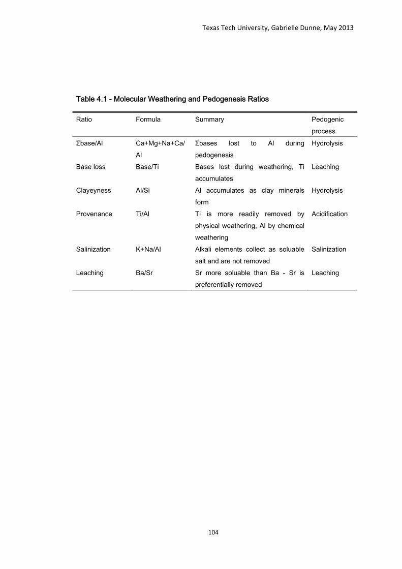
Texas Tech University, Gabrielle Dunne, May 2013
104
Table 4.1 - Molecular Weathering and Pedogenesis Ratios
Ratio Formula Summary Pedogenic process
Ʃbase/Al Ca+Mg+Na+Ca/Al
Ʃbases lost to Al during pedogenesis
Hydrolysis
Base loss Base/Ti Bases lost during weathering, Ti accumulates
Leaching
Clayeyness Al/Si Al accumulates as clay minerals form
Hydrolysis
Provenance Ti/Al Ti is more readily removed by physical weathering, Al by chemical weathering
Acidification
Salinization K+Na/Al Alkali elements collect as soluable salt and are not removed
Salinization
Leaching Ba/Sr Sr more soluable than Ba - Sr is preferentially removed
Leaching

Texas Tech University, Gabrielle Dunne, May 2013
105
Ratios between different elements can be used to evaluate pedogenic and
weathering processes in paleosols (Sheldon & Tabor, 2009). The following
paragraphs provide a summary of these relationships.
4.1.1 Barium/Strontium Ratio
Ba/Sr ratios can be used to estimate the intensity of leaching (Sheldon,
2006) and also the intensity of weathering (Kahmann et al., 2008). Higher
values of Ba/Sr indicate more leaching is taking place. Sr is significantly more
soluble than Ba and is therefore more readily leached (Sheldon and Tabor,
2009). Heavily leached paleosols are commonly characterized by a low Ba/Sr
ratio at the top of the horizon and a high Ba/Sr ratio at the bottom of the
horizon (Sheldon and Tabor, 2009). The ratio of Ba/Sr increases with the
duration of weathering and the degree of drainage, this ratio can range from
2; common in most rocks, up to 10; which is indicative of strongly leached
soils (Retallack, 1997).
4.1.2 Titanium/Zirconium
Ti and Zr are both relatively immobile elements (Sheldon and Tabor,
2009). This is due to the insoluble nature of the minerals in which they are
hosted i.e. Zr in Zircon (ZrSiO4) and Ti in rutile (TiO2) (Stiles, 2003). Zr is
more abundant in coarser fractions of sediment such as sands, while Ti is
more common in finer, clayey sediments; thus there exists a grain size factor
4.1 Weathering Ratios

Texas Tech University, Gabrielle Dunne, May 2013
106
on the ratio. Lower values of Zr are therefore indicative of removal through
physical weathering and the preferential removal of larger grains (Stiles,
2003). Zr is chemically immobile and only able to be redistributed and
accumulate through physical weathering processes, i.e. small additions of Zr
to the upper portion of soil are commonly the result of introduction of detrital
zircon by eolian processes (Stiles, 2003). Conversely, Ti elevated ratios are
indicative of illuviation of fine grained material downward through a soil profile
(Stiles, 2003). Ti/Zr ratios are also able to provide information on provenance,
a scatter plot of Zr against Ti which displays a linear trend would be indicative
of a homogeneous source (Kahmann et al., 2008). However, scatter plots of
data collected from our cores showed no significant correlations due to the
overprinting of grain size effects.
4.1.3 Aluminum/Silica
The Al/Si ratio indicates the degree of clay production by feldspar
weathering and clay translocation i.e. illuviation (Kahmann et al., 2008).
These values tend to range between 0.1 and 0.3, they may be very close to 0
in very sandy soils and above 0.3 in very clayey soils (Retallack, 1997);
largely due to the increased abundance of Al in clay minerals relative to a
silicate parent mineral (Sheldon and Tabor, 2009). Syn-formational addition
of Si may be attributed to the addition of eolian sediment (Sheldon and Tabor,
2009). These can be distinguished by other commonly observed trend in

Texas Tech University, Gabrielle Dunne, May 2013
107
eolian sediment i.e. increased Zr and by comparison to the element suite
observed in the Blackwater Draw Formation.
4.1.4 Alkaline/titanium ratios
These ratios indicate leaching, during weathering Na, K and Ca are leached
while the chemically immobile Ti remains (Sheldon and Tabor, 2009). In arid
setting, leaching is limited due to lack of moisture, in humid settings the
leaching of bases will be enhanced (Retallack, 1997) thus more leached soils
indicate humid conditions while less leached soils indicate arid conditions.
4.1.5 Potassium + Sodium/Aluminum
This ratio is used as an indicator of salinization, a subsurface enrichment of K
+ Na relative to Al is commonly found in paleosols which form in arid to desert
regions (Retallack, 1997). This indicator of aridity is often accompanied by
other aridity indicators such as the presence of carbonate nodules or other
evaporite minerals (Sheldon and Tabor, 2009).
4.1.6 Summation of Bases/Aluminum Ratio
This ratio uses ∑bases (i.e. Ca + Mg + Na + K), which are the primary
cations lost during weathering, plotted against Al. This indicates weathering
of paleosols through hydrolysis (Sheldon and Tabor, 2009). As climate
becomes warmer and wetter alkali earth elements become depleted at the
expense of refectory elements such as Al (Tabor et al., 2002).

Texas Tech University, Gabrielle Dunne, May 2013
108
4.1.7 Titanium/Aluminum
This ratio is most commonly used to determine provenance of the
parent material, but has also been linked to climatic variations (Boyle, 1983).
The Ti content varies significantly between different rock types while the
concentration of Al remains relatively stable (Sheldon and Tabor, 2009).
Mafic rocks generally display a high Ti/Al ratio while sandstones and
mudstones have a low Ti/Al value (Fig 4.1) adapted from Sheldon and Tabor,
(2009). Ti is often lost towards the top of soil profiles as a result of physical
weathering through processes similar to those discussed under the Ti/Zr ratio
(Sheldon and Tabor, 2009). In the marine realm, higher Ti/Al values have
been linked with oxygen isotopic excursions and have been found to correlate
to cold climates (Boyle, 1983). This largely reflects the addition of coarser,
wind-blown silt material during glacial periods.

Texas Tech University, Gabrielle Dunne, May 2013
109
Figure 4.1: Average Ti/Al ratios for paleosols with sandstones parent (Diamond), mudstone parent (triangles) and basalt parent (square). The highlighted section covers the range in which our results fall, adapted from Sheldon and Tabor (2009).

Texas Tech University, Gabrielle Dunne, May 2013
110

Texas Tech University, Gabrielle Dunne, May 2013
111
4.1.8 Carbonates
The presence of CaCO3 indicates aridity, CaCO3 is highly soluble thus
it is readily mobilized in ground water and soil solution, therefore it is removed
from the soil profile under humid conditions (Sheldon and Tabor, 2009). Table
4.2 adapted from Gile et al., (1966) demonstrates the various stages of
development of carbonates within arid and semi-arid soils. Using this
classification, soils with carbonate horizons in the playa cores studied are best
characterized as type II carbonate accumulations.
Nodular concretions of calcium carbonate form when Ca2+ ions from
precipitation of minerals in the soil combine with CO32- from precipitation, soil
minerals or root respiration (Barchardt and Lienkaemper, 1999). This process
is enhanced in arid and semi-arid climates; short periods of precipitation
encourage the dissolving stage these are followed by prolonged periods of
evapotranspiration which concentrate the nodules (Barchardt and
Lienkaemper, 1999). An abundance of carbonate in a horizon is termed a Bk
Horizon (Brady and Nyle, 2008).

Texas Tech University, Gabrielle Dunne, May 2013
112
Table 4.2 - Stages of Carbonate accumulation in soils
Stage Properties
I Didpersed powdery and filamentous carbonate.
II Few to common carbonate nodules and veinlets, with powdery and filamentous carbonate in places between nodules.
III Carbonate forming a continuous layer formed by coalescing nodules; isolated nodules and powdery carbonate outside the main horizon.
IV Upper part of the solid carbonate layer with a weakly developed platy or lamellar structure capping less pervasivley calcareous parts of the profile.
V Platy of lamellar cap to the carbonate layer strongly expressed; in places brecciated with pisolites of carbonate
VI Brecciation and recementation, as well as pisoliths, common in association with the lamellar upper layer.
adapted from Gile et al. (1966)

Texas Tech University, Gabrielle Dunne, May 2013
113
4.1.9 Iron-Manganese Nodules
Visible nodules of ferromanganese precipitated from extant pools of Fe
and Mn in the soil occur most commonly in finer grained, clayey sediments
with restricted permeability and drainage, in temperatures ranging from
continental warm to subtropical (Stiles et al., 2001). The formation of nodules
is controlled by seasonal wetting and drying in the vadose zone, Fe-Mn
nodules initially form as hydrous-phase assemblages in micropores and
accrete outwards (Stiles, 2001). The nodules form through dissolution and
precipitation along a redox gradient, MnO is first precipitated subsequent
oxidation of Fe2+ by the MnO results in the accretion of Fe3+ (Golden et al.,
1988).
The following section applies the theory described in the above section
to the results observed in these samples.
4.2.1 Bailey Playa-1
Figure 4.2 represents core BP-1, the Ba/Sr ratio remains fairly constant
throughout the modern soil and b1. Ba/Sr peaks in b2 in the Btcb2 horizon
above a Bk horizon, it is likely that re-deposition occurred on the surface of
4.2 Weatehring Profiles of Playa Sediments in BaileyCounty and Floyd County

Texas Tech University, Gabrielle Dunne, May 2013
114
Figure 4.2: Weathering ratios in BP-1 plotted against depth in cm, a
key for the symbols used in the stratigraphic log can be found in Figure
3.1. This core is fairly homogenous but shows leaching in the Ba/Sr
profile. The absence of leaching in the K, Na and Ca/Ti profiles is
indicative of arid conditions.

Texas Tech University, Gabrielle Dunne, May 2013
115

Texas Tech University, Gabrielle Dunne, May 2013
116
the Bk. The Ba/Sr ratio is lower at the top (~5) of Btcb2 and higher (>10) at
the bottom of Btcb2, this is indicative of a heavily leached soil (Sheldon and
Tabor, 2009). Another smaller peak is observed at S3 indicating that the soil
Bmcb2 may also be leached. The values in this core are moderately high >5
this indicates that leaching is likely taking place throughout the soil profiles.
Ti/Zr shows fluctuation throughout the modern soil, moving up through
b2 and b1 Ti increases in abundance relative to Zr indicating physical
weathering processes. Zr is contained in larger sandy grains thus, it may be
inferred that preferential removal of these sandy grains by eolian processes
account for the depletion in Zr. Soil b3 shows a large influx of Zr at the
surface, this may be due to an increase in illuviation of Ti bearing fines at this
time. Alternatively, and more likely, this increase in Zr may be due to an influx
of eolian material containing detrital zircon (Stiles, 2003). Ti /Zr can also be
used as an indicator of provenance however much of the literature (e.g.
Holliday, 1989) report that the Blackwater Draw Formation is the primary
sediment source in this area. Differences observed in the Ti/Zr ratios of each
horizon may be an artifact of changes in grain size i.e. larger grains higher Zr
concentration, smaller grains higher Ti concentration. The increase in grain
size observed through soil b2 is tracked by enrichment in Zr.
Al/Si demonstrates enrichment of Al relative to Si in b3, towards the top
of Btb3 the Al/Si value is <0.1, this is considered to be very sandy (Retallack,

Texas Tech University, Gabrielle Dunne, May 2013
117
1997). Above S3, a prolonged positive trend of Al enrichment relative to Si is
observed which continues across S1 and S2 all the way up to the upper 15cm
(modern soil) where the positive trend steepens indicating an increase in clay
content of the soils above S3.
Na, K and Ca all become enriched relative to Ti at S3 indicating a small
degree of leaching took place at this time. Leaching of these bases requires
moisture (Retallack, 2001b), however minimal moisture is likely in this interval
due to the low degree of leaching. Throughout the rest of the core no
leaching profiles are observed this may indicate that moisture levels are
insufficient for the leaching of these soluble bases.
Figure 4.3 shows the K+Na/Al, Ʃbases/Al andTi/Al ratios. The increase
in K + Na relative to Al observed at S3 indicates that salinization may have
occurred through b2 and the K and Na accumulated on S3.
Ʃbases/Al show an increase in abundance of Ʃbases relative to Al
above S3 indicating hydrolysis occurred through the formation of b2. Thus,
moisture must have been sufficient to dissolve Mg, Ca, Na and K ions from
the parent silicate mineral. Above S2, no trends are seen indicating little to no
hydrolysis was taking place, thus arid conditions may have been likely.
The presences of Bk horizons indicate arid to semi-arid conditions as CaCO3
is too soluble to remain in humid conditions (Sheldon and Tabor, 2009).

Texas Tech University, Gabrielle Dunne, May 2013
118
Figure 4.3: Weathering ratios in BP-1 plotted against depth in cm, a
key for the symbols used in the stratigraphic log can be found in Figure
3.1. These again show few major trends. Salinization may be
observed at S3.

Texas Tech University, Gabrielle Dunne, May 2013
119

Texas Tech University, Gabrielle Dunne, May 2013
120
The presence of ferromanganese nodules between 280 cm and 190 cm is
troubling as they are largely reported under wetter climate regimes (Stiles et
al., 2001) and reasons for the seemingly inconsistent carbonate and Fe-Mn
intercalated nodule bearing horizons is unclear. Soil horizons such as this
which contain both carbonate and Fe-Mg nodules have been observed to infer
seasonality in monsoonal climates, where carbonate nodules form during the
dry season and Fe-Mn nodules for during the wet season (Sehgal and
Stoopes, 1972).
4.2.2 Bailey Playa -2
Figures 4.4 and 4.5 represent the weathering profiles of core BP-2. The
Ba/Sr ratio demonstrates leaching in Bcb3 and Bkb1 i.e. higher ratios at the
bottom of the horizon relative to the top. The Btcb1 horizon demonstrates a
large peak at the top of this horizon; this accumulation may be the result of
illuviation.
Ti/Zr fluctuates throughout the core and is likely a function of grain size;
observed increases in grain sizes can be correlated with an increase in the
abundance of Zr relative to Ti. Al/Si remains relatively constant throughout
the whole core. The Al/Si value is around 0.2 indicating that the sediment is a
mixture of sand and clay (Reatallack, 1997) consistent with the grain size
distributions presented earlier.
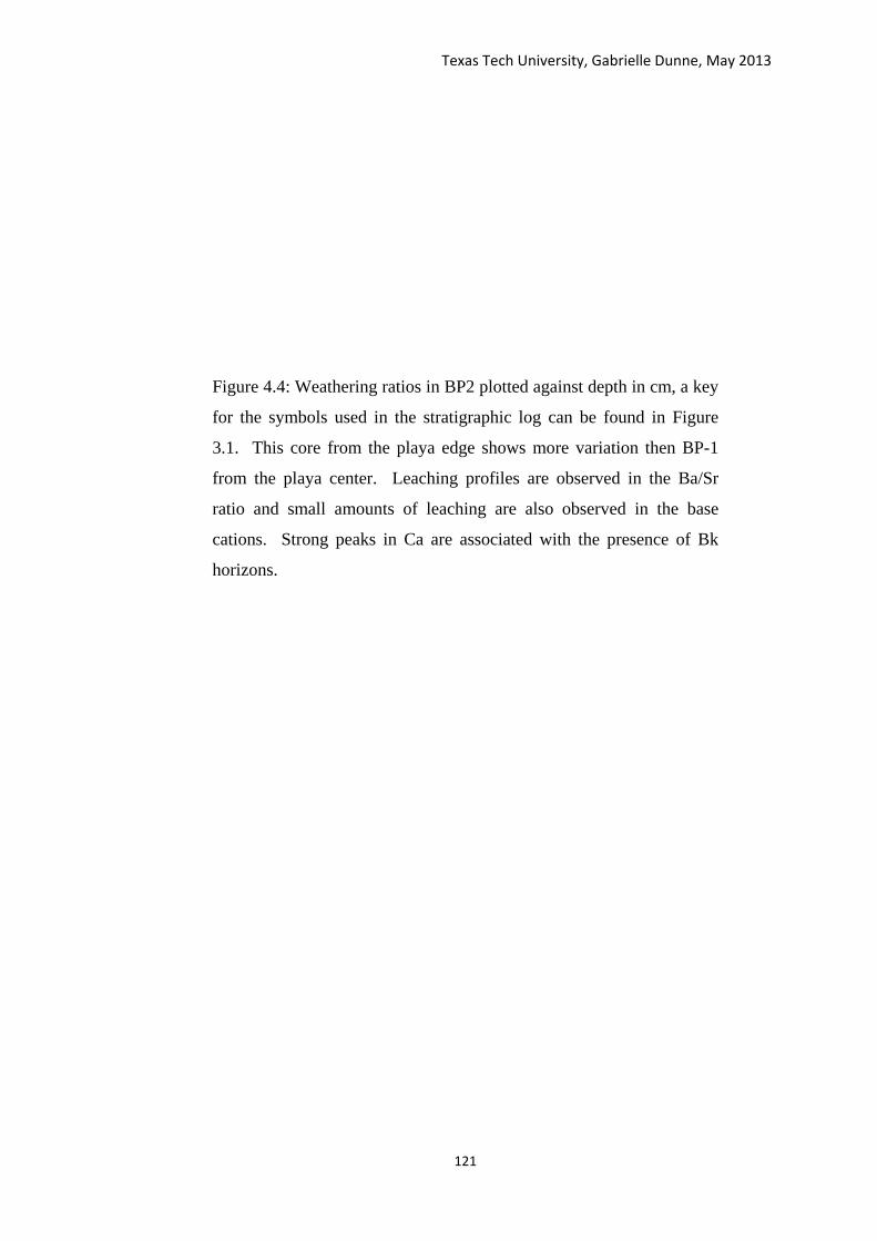
Texas Tech University, Gabrielle Dunne, May 2013
121
Figure 4.4: Weathering ratios in BP2 plotted against depth in cm, a key
for the symbols used in the stratigraphic log can be found in Figure
3.1. This core from the playa edge shows more variation then BP-1
from the playa center. Leaching profiles are observed in the Ba/Sr
ratio and small amounts of leaching are also observed in the base
cations. Strong peaks in Ca are associated with the presence of Bk
horizons.

Texas Tech University, Gabrielle Dunne, May 2013
122

Texas Tech University, Gabrielle Dunne, May 2013
123
Figure 4.5: Weathering ratios in BP2 plotted against depth in cm, a key
for the symbols used in the stratigraphic log can be found in Figure
3.1. An overall depletion of the ∑bases relative to Al is observed
indicating conditions were too moist for salinization to occur.

Texas Tech University, Gabrielle Dunne, May 2013
124

Texas Tech University, Gabrielle Dunne, May 2013
125
The Na/Ti, K/Ti and Ca/Ti are fairly constant indicating that little
leaching has taken place. Thus, it can be inferred that moisture was
insufficient for the removal of these bases i.e. conditions were arid.
Accumulations of Ca are associated with the presence of Bk horizons, again
indicate climatic aridity (Sheldon and Tabor, 2009).
Salinization trends are observed through b2, b1 and the modern soil
i.e. K + Na is enriched relative to Al towards the bottom of each profile. Thus
arid desert like conditions with a low Mean Annual Temperature may be
inferred (Sheldon and Tabor, 2009).
Fluctuations observed in Ʃbases/Al are most likely an artifact of the
fluctuations in Ca related to the presence of Bk horizons. The overall trend in
the core is a depletion in bases relative to Al upward through b2 and b3
indicating a warming and wetting of climate (Sheldon et al., 2002). Ti/Al is
used to determine provenance, Ti/Al values are low, <0.1 this is indicate that
the likely source is a sandstone or mudstone (Fig 4.1).
Carbonate nodules are present in three of the horizons; Bkb3, Bckb2
and Bkb1 indicating some degree of aridity. Ferromanganese nodules are
present in Bcb3, BcKb2 and Btcb1 indication poorly developed drainage
(Stiles 2001.) Soil horizons such as Bckb2 which contain both carbonate and
Fe-Mg nodules formed by intermittent intergrowth have been observed to infer
seasonality in monsoonal climates, where carbonate nodules form during the

Texas Tech University, Gabrielle Dunne, May 2013
126
dry season and Fe-Mg nodules for during the wet season (Sehgal and
Stoopes, 1972).
4.2.3 Floyd Playa-1
Figure 4.6 and 4.7 show the weathering profiles for core FP-1 which is
from the center of the playa floor in Floyd County. This core is very
homogenous and exhibits little signs of weathering. The Ba/Sr profile shows
some leaching occurred through the Btcb1 and Bt Horizons. Ti/Zr shows
small fluctuations, these are likely an artifact of changes in grain size. K/Ti,
Na/Ti and Ca/ Ti remain constant, other than enrichment in Ca associated
with the Bk horizon. This indicates insufficient moisture for leaching of these
cations (Retallack, 1997). Al/Si gives a consistently low value indicative of a
sandstone or mudstone source (Sheldon and Tabor, 2009).
4.2.4 Floyd Playa-2
Figures 4.8 and 4.9 demonstrate the weathering profiles for the core
FP-2. The Ba/Sr ratios are indicative of leaching, particularly in the Bht
horizon of the modern soil. Strongly leached horizons tend to exhibit
accumulations of Ba/Sr relative to Sr towards the bottom of a horizon
(Sheldon and tabor, 2009) consistent with the large spike observed at 190 cm.
The Ti/Zr ratio exhibits enrichment in Zr associated with the C horizon this is
an artifact of grain size as horizon C contains predominantly sand material

Texas Tech University, Gabrielle Dunne, May 2013
127
Figure 4.6: Weathering ratios in FP-1 plotted against depth in cm, a
key for the symbols used in the stratigraphic log can be found in Figure
3.1. This core from the playa center is very homogenous. Leaching is
present in the Ba/Sr profile.

Texas Tech University, Gabrielle Dunne, May 2013
128

Texas Tech University, Gabrielle Dunne, May 2013
129
Figure 4.7: Weathering ratios in FP-1 plotted against depth in cm, a
key for the symbols used in the stratigraphic log can be found in Figure
3.1. Due to the cores homogeneity no significant trends are observed.

Texas Tech University, Gabrielle Dunne, May 2013
130

Texas Tech University, Gabrielle Dunne, May 2013
131
Figure 4.8: Weathering ratios in FP-2 plotted against depth in cm, a
key for the symbols used in the stratigraphic log can be found in Figure
3.1. Significant changes in the weathering profile are observed in the
C horizon as this is largely unweathered material. Above the C
horizon, a large accumulation of Na is observed with a smaller
accumulation of Ca. This may be the result of arid conditions,
insufficient moisture allowed these soluble cations to accumulate.

Texas Tech University, Gabrielle Dunne, May 2013
132
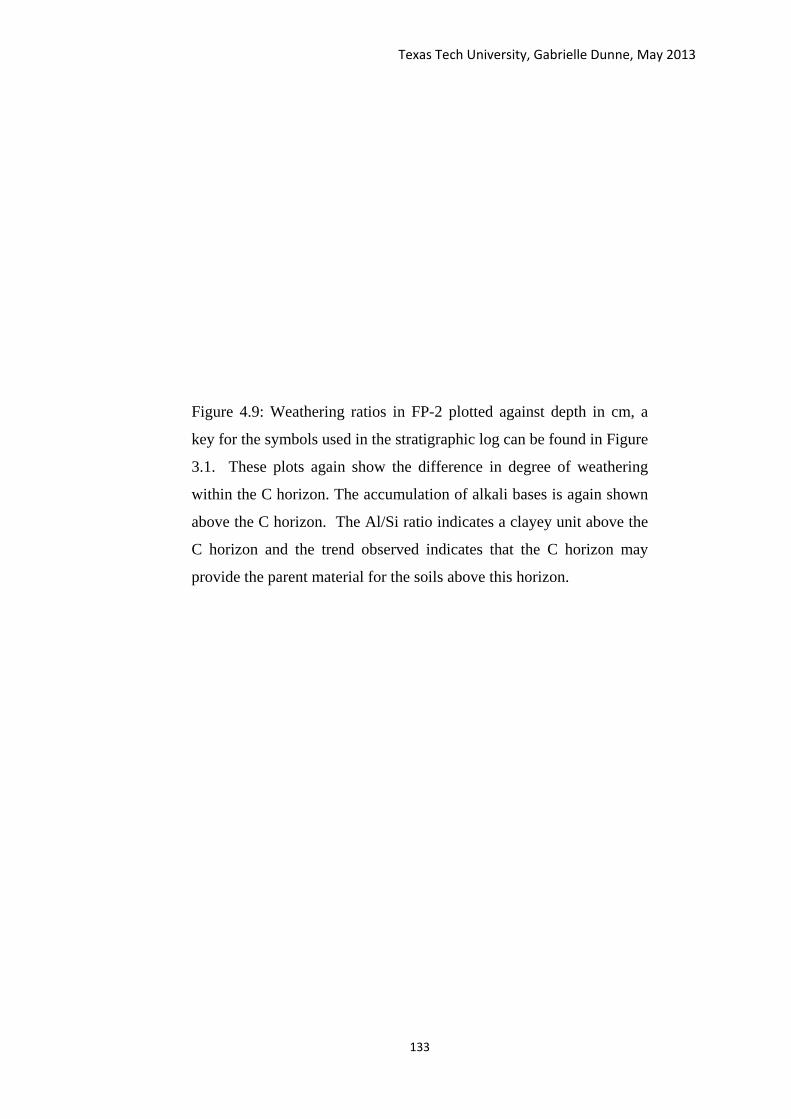
Texas Tech University, Gabrielle Dunne, May 2013
133
Figure 4.9: Weathering ratios in FP-2 plotted against depth in cm, a
key for the symbols used in the stratigraphic log can be found in Figure
3.1. These plots again show the difference in degree of weathering
within the C horizon. The accumulation of alkali bases is again shown
above the C horizon. The Al/Si ratio indicates a clayey unit above the
C horizon and the trend observed indicates that the C horizon may
provide the parent material for the soils above this horizon.

Texas Tech University, Gabrielle Dunne, May 2013
134

Texas Tech University, Gabrielle Dunne, May 2013
135
The Al/Si also shows an increase at the C horizon that can be attributed to a
higher proportion of silicate sand material.
Above the C horizon, the Na/Ti shows an accumulation of Na at the
bottom of the Btkb1, Btb1 and Bt horizons. This is likely due to leaching of
soluble salts such as Na from horizons above and their accumulation at intra-
soil horizon boundaries. K/Ti and Ca/Ti show similar yet less pronounced
trends. A strong peak in Ca/Ti is associated with Bkb2, the presence of this
Bk horizon indicates aridity.
Increases in the concentrations of Na+K/Al at the base of the Btkb1
horizon are likely the result of hydrolysis indicating climate was warm and
moisture was sufficient to dissolve the soluble K+ and Na+ cations and
redeposit them above the C horizon.
The Ʃbases/Al show that weathering through hydrolysis occurred in horizons
Btkb1 and Btb1 the Ʃbases become depleted with respect to Al up the profile
suggesting a warming and wetting of climate. The spike in the Bkb2 horizon
is related to the abundance of carbonate nodules which form the Bk horizon.
The Ti/Al ratio through the b1 soil shows a general decrease upward in Ti.
The highly elevated Al values just atop the C horizon are likely the result of
accumulation of illuviated clay minerals. However, if those values are
disregarded due to the illuviation mechanism rather than weathering, then the
Ti/Al trend forms a fairly consistent linear decrease upward; an expected trend

Texas Tech University, Gabrielle Dunne, May 2013
136
from parent material to daughter soil (Fig. 4.1, Sheldon and Tabor, 2009).
Thus, the b1 soil in FP-2 is the only soil horizon recovered, from any core, that
appears to show the relatively unweathered parent material and overlying soil.
4.2.5 Other Elemental Weathering Trends
BP-1 (Fig 3.10) displays an overall decrease in Zn, V and Cr towards
the surface. Zn and Cr are commonly associated with organic matter, along
with smaller quantities of V and may provide a proxy for former organic matter
in the paleosol profile (Retallack, 1990). Thus, this trend may be interpreted
as a decrease in organic matter moving up the profile. FP-1 (Fig 3.12) shows
a major spike in Cu and a smaller associate spike in Zn at S1, this spike in Cu
seems un-naturally large and is confined to a very small zone in the soil. It is
reasonable to assume this is a result of human activity i.e. copper pipes rather
than a pedogenic process.
4.2.6 Soil Characteristics
The horizons observed may also be classified as diagnostic horizons,
also known as epipedons which include both the darker, organic upper part of
the soil and the upper eluvial horizon (Brady & Weil, 2008). These are
summarized in table 4.3 and table 4.4, adapted from Brady & Weil (2008).

Texas Tech University, Gabrielle Dunne, May 2013
137
Table 4.3 - Surface Horizons
Diagnostic Horizon
Major features
Anthropic (A)
Human modified, mollic-like horizon, high in available P.
Folistic (O) Organic horizon saturated for <30 days/ normal year.
Histic (O) Very high in organic content, wet during some parts of the year.
Melanic (A) Thick, black, high in organic content (>6% organic C) common in volcanic ash soil.
Mollic (A) Thick, dark-colored, high base saturation, strong structure.
Orchic (A) Too light-colored or too low in organic content to be Mollic, may be hard and massive when dry.
Plaggen (A)
Human made soda-like horizon created by years of manuring.
Umbric (A) Same as Mollic except low base saturation.

Texas Tech University, Gabrielle Dunne, May 2013
138
Table 4.4 - Subsurface Horizon
Diagnostic Horizon
Major features
Argic (A or B) Organic and clay accumulation just below plow layer resulting from cultivation.
Albic (E) Light-colored, clay and Fe and Al oxides mostly removed. Argillic (Bt) Silicate clay accumulation. Calcic (Bk) Accumulation of CaCO3 or CaCO3.MgCO3 Cambic (Bw, Bg)
Change or altered by physical movement or chemical reactions, generally non-illuvial.
Duripan (Bqm)
Hard pan, strongly cemented silica.
Fragipan (Bx) Brittle pan, usually loamy textured, dense, coarse prisms. Glossic (E) Whiteish eluvial horizon that tongues into Bt Gypsic (By) Accumulation of gypsum. Kandic (Bt) Accumulation of low-activity clays. Natric (Btn) Argillic, high sodium, columnar or prismatic structure.
Oxic (Bo) Highly weathered, primarily mixture of Fe, Al oxides and nonsticky-type silicate clays.
Petrocalcic (Ckm)
Cemented calcic horizon
Petrogypsic (Cym)
Cemented gypsic horizon.
Placic (Csm) Thin pan cemented with Fe alone, or with Mn .or organic matter Salic (Bz) Accumulation of salts. Sombric (Bh) Organic matter accumulation. Spodic (Bh, Bs)
Organic matter, Fe, Al oxide accumulation
Sulfuric (C) Highly acidic with Jarosite mottles.

Texas Tech University, Gabrielle Dunne, May 2013
139
4.3.1 Bailey Playa
The modern soil and b1 soil in the Bailey Playa are primarily Bt or Bk
with some modifications such as nodules (c), color structure (w) or illuvial
accumulations (h) and (t). These are interpreted as Mollisols. Molisols
generally form on flat low lying land, with sub-humid to semi-arid climates and
support grassland vegetation (Retallack, 1990). Leaching near the
subsurface and illuviation leading to clay enrichment in the Bt horizon, along
with the removal of Ca+, Na+, K+ and Mg+ by hydrolysis indicate that a
Lessivage soil forming regime may be present (Retallack, 1990). Additionally,
the b1 soil contains calcic sub horizons suggesting that the climate during that
interval was slightly more arid than the modern climate. The characteristics of
the soils observed within the modern profile are very similar to those observed
by Holliday et al., (2008) in the Randall Clay, present in nearby playas. Thus
we infer the modern profile is part of this formation. The characteristics of the
soil in b1 is similar to those observed by Holliday et al., (2008) in the Tahoka
Formation of playa located close by, thus it can be inferred b1 is part of the
Tahoka Formation.
Soil b2 observed in the Bailey Playa cores is less well developed and
contains some degree of subsurface clay accumulation, but overall poor
horizonation. Thus, these soils are best characterized as Inceptisols.
4.3 Correlation and Soil Types

Texas Tech University, Gabrielle Dunne, May 2013
140
Inceptisols are able to form in a range of climates and vegetation, but
commonly form in open grasslands (Retallack, 1990). Moreover, both the BP-
1 and BP-2 cores contain fairly well developed Bk and less developed Bt
horizons indicating more aridity than the overlying soils. The characteristics of
this soil are again similar to the Tahoka Formation described by Holliday et
al., (2008) thus we b2 is inferred to form part of the Tahoka Formation.
Soil b3 in the Bailey Playa is largely characterized as a well-developed
Bk horizon in the BP-2 core and a Bt horizon in the centrally located BP-1
core. The entire soil profile was not penetrated during coring, but based on
the well-developed Bk horizon in the BP-2 core, an aridisol soil series is
inferred for the interval. This soil is likely derived from the Blackwater Draw
Formation as Holliday et al., (2008) observe the Tahoka Formation lies atop
Blackwater Draw sediments.
In summary, the Bailey Playa soils observed in core change from
Aridisol to Inceptisol to Mollisol upwards (Fig 4.10). This trend in soil series
types can generally be related to an increase upward in precipitation and
possibly temperature.

Texas Tech University, Gabrielle Dunne, May 2013
141
Figure 4.10: Correlation between sediments from the center of the
playa floor and sediment from the playa margin for the Bailey County
Playa. A key to the symbols used in the stratigraphic log can be found
in Fig 3.1.

Texas Tech University, Gabrielle Dunne, May 2013
142
Texas Tech University, Gabrielle Dunne, May 2013
143
4.3.2 Floyd Playa
The modern soil in the Floyd Playa are primarily Bt or Bht, these are
interpreted as Mollisols thus flat low lying land, with sub-humid to semi-arid
climates and grassland vegetation may be inferred (Retallack, 1990).
Leaching near the subsurface and illuviation leading to clay enrichment in the
Bt horizon along with the removal of Ca+, Na+, K+ and Mg+ by hydrolysis
indicate that a lessivage soil forming regime may be present (Retallack,
1990).
The characteristics of the soils observed within the modern profile are
very similar to those observed by Holliday et al., (2008) in the Randall Clay,
present in nearby playas. Thus we infer the modern profile is part of this
formation.
Soil b1 observed in the Floyd county playa exhibits clay accumulation,
the development of horizonation decreases with depth through b1. These
soils are characterized as Mollisols at the top, thus climates which support
grassland may be inferred (Retallack, 1990). However, the S2 surface likely
indicates a second soil forming episode with poor horizonation and is inferred
as an Inceptisol. The sandy unit observed in FP-2 is interpreted as an influx
of fluvial deltaic sediment, similar to the gravel/sand member of the Tahoka
Formation observed by Hall (2001). The clay portion of this unit displays
characteristics very similar to those observed by Holliday et al., (2008) in the

Texas Tech University, Gabrielle Dunne, May 2013
144
Tahoka Formation of playa located close by, thus it can be inferred b1 is part
of the Tahoka Formation.
Soil b2 in the Floyd contains well-developed Bk horizon, Fe-Mn concretions
are also present. The entire soil profile was not penetrated during coring,
but based on the well-developed Bk horizon, an aridisol soil is inferred for this
interval. This soil is likely derived from the Blackwater Draw Formation as
Holliday et al., (2008) observe the Tahoka Formation atop Blackwater Draw
sediments.
Floyd Playa soils also exhibit a change from Aridisol to Inceptisol to
Mollisol upwards (Fig 4.11). This trend in soil series types can generally be
related to an increase upward in precipitation and possibly temperature as
well.

Texas Tech University, Gabrielle Dunne, May 2013
145
Figure 4.11: Correlation between sediments from the center of the
playa floor and sediment from the playa margin for the Floyd County
Playa. A key to the symbols used in the stratigraphic log can be found
in Fig 3.1.

Texas Tech University, Gabrielle Dunne, May 2013
146

Texas Tech University, Gabrielle Dunne, May 2013
147
4.3.3 Playa formation considerations
Figure 4.10 demonstrates the correlation between the facies observed
at the playa center and playa edge for the Bailey Playa. The Randall Clay
appears to be thicker at the playa edge (BP-2) than in the playa center (BP-1).
This may be the result of increased accommodation space at the playa edge
relative to the playa center, this is concurrent with Wood and Osterkamp’s
(1987a) model of playa enlargement through dissolution, whereby playas
enlarge from the center outwards, thus the annular becomes the main zone of
recharge (Wood & Osterkamp 1987a). Randall Clays are known to form
under ponded conditions or heavily vegetated sub-aerial conditions (Holliday
et al., 2008).
The Tahoka Formation which forms soils b1 and b2 is thicker at the
center of the playa indicating greatest subsidence here this may be a result of
dissolution of carbonate below by precipitation and ground water runoff which
may have accumulated in the initial depression (Wood & Osterkamp 1987a).
The Pale olive gray clays observed in this section of the Tahoka Formation
are lacustrine muds which may have formed during periods of playa
inundation (Holliday et al. 2008). Below this both cores reach the Blackwater
Draw Formations uppermost Aridisol.

Texas Tech University, Gabrielle Dunne, May 2013
148
Figure 4.11 demonstrates the correlation between the facies observed
at the playa center and playa edge for the Floyd County Playa. The Randall
Clay appears to be thicker at the playa edge (FP-2) than in the playa center
(FP-1). This may be the result of increased accommodation space at the
playa edge relative to the playa center, and is again concurrent with Wood
and Osterkamp’s (1987a) model of playa enlargement through dissolution at
the annulus. Both facies of the Tahoka Formation are present in b1, FP-1 is
composed only of the lacustrine muds, FP-2 however exhibits an influx of
sand and gravel known to occur in the playa margin this is interpreted as a
fluvial-deltaic sediment (Evans & Meade, 1945). Below the Tahoka formation,
FP-2 extends in to the Blackwater Draw Formations uppermost Aridisol.
The Blackwater Draw Formation exhibits a well-established northerly
fining trend (Fig 4.12) adapted from Holliday, (1989). Various grain size
relationships show remarkable correlation (often R2 = .88 to .94) with distance
from the Pecos River located to the south of the Southern High Plains (Fig.
4.13 & 4.14; Holliday, 1989). Deviations from this trend would indicate either a
different source than the Blackwater Draw Formation or hydrological
reworking of the Blackwater Draw Formation after deposition. However,
within the study areas the Blackwater Draw Formation is the only viable
source as it represents the surface that the playas formed on and exterior
4.4 Temporal Constraints

Texas Tech University, Gabrielle Dunne, May 2013
149
sediment sources to the Southern High Plains have not existed since the
Pecos River down-cut to the west and isolated the region around 1.6 Ma
(Holliday, 1989). Therefore, grain size parameters that are significantly
deviated from the well-established trends shown in the Blackwater Draw
Formation would indicate reworking of the Blackwater draw Formation and
thus, a relatively younger age.
In the Bailey Playa cores, grain size data was taken from 40-100 cm
below the S2 surface and results indicate that the BP-1 core is significantly
elevated (i.e. close to or more than 1 σ) in sand percentage and mean sand
size (Fig. 4.13). Moreover, the BP-2 data shows a standard deviation less
very fine sand to silt ratio. In the Floyd Playa cores, grain size data was taken
from 70-130 cm below the S1 surface and results here indicate that both
cores show significant departure from the observed trend in the Blackwater
Draw Formation (Fig. 4.14).

Texas Tech University, Gabrielle Dunne, May 2013
150
Figure 4.12 adapted from Holliday, 1989 demonstrates the northerly
fining of grains size with distance from the Pecos River.

Texas Tech University, Gabrielle Dunne, May 2013
151

Texas Tech University, Gabrielle Dunne, May 2013
152
Figure 4.13: S-N transect of a) % sand (R2 = 0.88), b) mean sand (mm;
R2 = 0.93) and c) very fine sand versus coarse silt (vfs/silt; R2 = 0.31)
against distance (km) from the Pecos River. BP-1 (green square) and
BP-2 (orange square) are plotted along with margins of ±1σ (dashed
lines).

Texas Tech University, Gabrielle Dunne, May 2013
153

Texas Tech University, Gabrielle Dunne, May 2013
154
Figure 4.14: SW-NE transect of a) % sand (R2 = 0.94), b) mean sand
(mm; R2 = 0.94) and c) very fine sand versus coarse silt (vfs/silt; R2 =
0.58) against distance (km) from the Pecos River. FP-1 (green square)
and FP-2 (orange square) are plotted along with margins of ±1σ
(dashed lines)

Texas Tech University, Gabrielle Dunne, May 2013
155

Texas Tech University, Gabrielle Dunne, May 2013
156
Results relatively consistent with the trends are not meaningful to
interpret as either original Blackwater Draw Formation or reworked Blackwater
Draw Formation because both scenarios could produce results on that trend.
However, results outside of the ±1σ are significant and hard to reconcile as
original Blackwater Draw Formation. Thus, the most likely scenario is the b2
soil in the Bailey Playa is post-youngest age for the Blackwater Draw
Formation. Thermoluminescence and radiocarbon dating typically bracket a
minimum age for the Blackwater Draw Formation between 40 and 30 ky
(Holliday, 1989; Holliday et al., 1996; Holliday et al., 2008) .Thus, the
paleosols studied here are younger than ~ 40ky.
A more refined temporal constraint can be derived from the
comparison of our soils with similar soils of other studies. Holliday et al.,
(2008) carried out a sedimentological study of 30 different playa fills on the
Southern High Plains. Two of the playas which they sampled were very
close in location to our sample locations; Colston Playa (11) is ~18 km
north of Floyd Playa and Radcliffe Playa (19) is ~18 km southwest of
Bailey Playa. Both of the Bailey and Floyd Playas contain horizons
sedimentologically similar to the Tahoka Formation observed in the
Colston and Radcliffe Playas. Holliday et al., (2008) use 14C dating to
provide an estimate for the age of the Tahoka Formation. The Tahoka
Formation clays in Colston Playa were dated at 11,570 14C yrs BP in the
Texas Tech University, Gabrielle Dunne, May 2013
157
upper part of the section, thus is may be possible that uppermost Tahoka
Formation in the Floyd and Bailey Playas are of a similar age. In the
Radcliffe Playa, the lowermost part of the Tahoka Formation were dated at
21,360 14C yrs BP, thus it may be possible that the lower section of the
Tahoka Formation in Bailey and Floyd Playas are of a similar age.
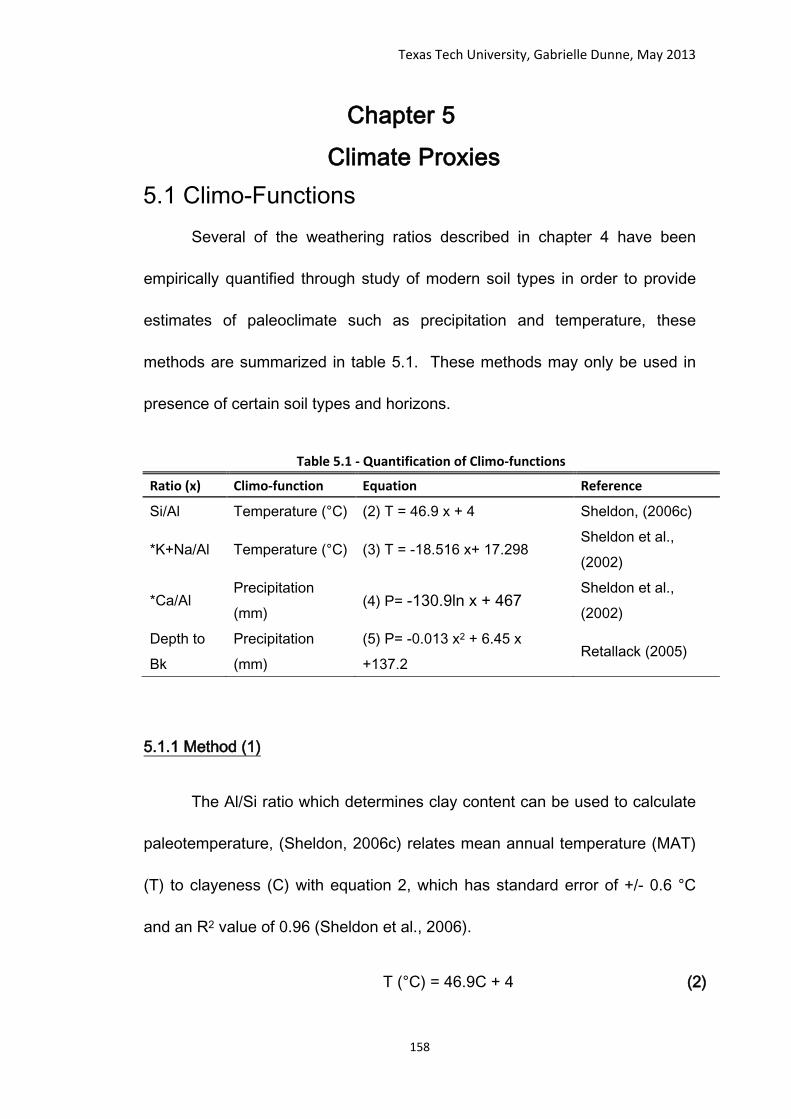
Texas Tech University, Gabrielle Dunne, May 2013
158
Chapter 5Climate Proxies
Several of the weathering ratios described in chapter 4 have been
empirically quantified through study of modern soil types in order to provide
estimates of paleoclimate such as precipitation and temperature, these
methods are summarized in table 5.1. These methods may only be used in
presence of certain soil types and horizons.
Table 5.1 - Quantification of Climo-functions
Ratio (x) Climo-function Equation Reference
Si/Al Temperature (°C) (2) T = 46.9 x + 4 Sheldon, (2006c)
*K+Na/Al Temperature (°C) (3) T = -18.516 x+ 17.298 Sheldon et al., (2002)
*Ca/Al Precipitation (mm)
(4) P= -130.9ln x + 467 Sheldon et al., (2002)
Depth to Bk
Precipitation (mm)
(5) P= -0.013 x2 + 6.45 x +137.2
Retallack (2005)
5.1.1 Method (1)
The Al/Si ratio which determines clay content can be used to calculate
paleotemperature, (Sheldon, 2006c) relates mean annual temperature (MAT)
(T) to clayeness (C) with equation 2, which has standard error of +/- 0.6 °C
and an R2 value of 0.96 (Sheldon et al., 2006).
T (°C) = 46.9C + 4 (2)
5.1 Climo-Functions

Texas Tech University, Gabrielle Dunne, May 2013
159
This method is applicable only to the Bt and Bw horizons of inceptisols
(Sheldon, 2006c). Thus, the method can be applied to the Bt and Bw
horizons of buried soil 2 in cores BP-1 and BP-2 and buried soil 2 in FP-1
(Table 5.2).
5.1.2 Method (2)
Sheldon et al., (2002) relate salinization trends to MAT °C (T) using the
molecular ratios of Na2O +K2O/Al2O3 (S) (equation 3). Na and K tend to
accumulate in desert environments thus a low MAT would be expected for
horizons which demonstrate salinization (Sheldon & Tabor, 2009). This
method has a standard error of +/- 4.4 °C, an R2 value of 0.37 and is
significant to the 99.9% level (Sheldon et al., 2002).
T (°C) = -18.516(S) + 17.298 (3)
This method is only applicable to lowland soils formed within the last
100 ky under climates that have a MAT range of 2-20°C (Sheldon et al., 2002)
thus it will be applicable to this study. The equation may only be applied to Bt
and Bw horizons that exhibit significant salinization trends i.e. a subsurface
enrichment of Na + K relative to Al, and yields best results when applied to
Inceptisols (Sheldon et al., 2002). The only horizon suitable for this analysis
is Btcb2 in core BP-1 (Table 5.2).

Texas Tech University, Gabrielle Dunne, May 2013
160
Table 5.2 - Summary of paleotemperature
Method: (1) Al/Si T (°C) = 46.9C + 4
Core Horizon Depth (cm) Temperature (°C) BP-1 Btcb2 220 14.2
230 14.2
240 13.6
Average 14
Btkb2 250 13.9
260 13.2
Average 13.6 BP-2 Btb2 220 12.0
230 11.9
Average 11.95 FP-1 Bwkb2 310 15.8
320 15.9
330 15.9
340 16.0
Average 15.9 Method: (2) Salinization T (°C) = -18.516(S) +
17.298
Core Horizon Depth (cm) Temperature (°C) BP-1 Btcb2 230 13.5
240 13.5
Average 13.5 FP-2 Btb1 230 12.9
240 12.9 250 12.9 260 12.6 270 12.4 Btkb1 280 12.6 290 12.5 300 12.6 310 12.5 Average 12.6

Texas Tech University, Gabrielle Dunne, May 2013
161
5.1.3 Method (3)
Sheldon et al., (2002) propose a proxy for MAP which utilizes the molar
ratio of Ca/Al (C) (Equation 4). This method has a standard error of +/- 156
mm and an R2 =0.59. This relationship is applicable only to Mollisols in the B
horizon where significant variation from the weathering ratio of the parent
material is observed (Sheldon et al., 2002). Following these limitations this
method may be applied the horizons Btb1 and Btkb1 in core FP-2 (Table 5.3).
P (mm/yr) = -130.9ln (C) + 467 (4)
These relationships are applied on to Bt and Bw horizons as they form
over longer time periods and are in equilibrium with the climate (Sheldon &
Tabor, 2009). The longer period of formation also ensures that short time
climate trends such as those associated with El Nino events do not impose on
the long-term trends (Sheldon &Tabor, 2009).
5.1.4 Method (4)
The depth of the Bk horizon (D) is also correlated with the MAP this
relationship is quantified by equation 5 adapted from Retallack, (2005). This
relationship was determined using data collected by Jenny and Leonard
(1935) from 807 globally distributed soils. This method has a standard error
of ±147 mm yr−1, and R2=0.52 (Retallack, 2005).
P (mm/yr) = -0.013D2 + 6.45D +137.2 (5)

Texas Tech University, Gabrielle Dunne, May 2013
162
In sub-humid regions the Bk horizon is generally deep but in arid
regions Bk horizons are much shallower (Retallack, 2005). In warm and wet
climates, bases such as Calcium are readily removed, in more arid regions
moisture is insufficient to remove Calcium cations, thus they accumulate at
the upper surface of Bk horizons (Sheldon et al., 2002).
This method has been applied to soils ranging in age from the Paleozoic to
the Quaternary (Retallack, 2001b). When applying this relationship pre-burial
erosion, post-burial compaction and atmospheric CO2 levels must be
considered, however these are generally not an issue when dealing with post-
Cretaceous soils (Berner and Kothavala, 2001). This relationship may only be
applied to moderately developed soils which contain calcite nodules in
Table 5.3 - Summary of paleoprecipitation
Method (4) P = -130.9ln (Ca/Al) + 467
Core Horizon Depth (cm)
Precipitation (mm/yr)
FP-2 btb1 230 181
240 163
250 162
260 206
Average 178
Btkb1 270 215
280 182
290 237
300 234
310 255
Average 225

Texas Tech University, Gabrielle Dunne, May 2013
163
lowland setting with limited human disturbance (Sheldon &Tabor, 2009), thus
this method will be applicable to all the cores which contain Bk horizons
(Table 5.4).
The modern MAT on the Southern High Plains is 18.6°C (High Plains
Regional Climate Centre, 2009). Using Method 1 to calculate temperature
results in a temperature range between ~12-16°C, these are cooler than
modern temperatures (Fig. 5.1). Method 2 gives results which are very
consistent with those observed at the same depth in BP-1, the average
temperature for soil b1 is 13.5°C this is ~ 5°C cooler than present. The
convergence of the two methods around a similar temperature strengthens
the argument that the numbers are valid. The sediments from which these
values were calculated form part of the Tahoka formation, dated around
Table 5.4 - paleoprecipitation calculated using depth to Bk Method (4): P (mm/yr) = 0.013D2 + 6.45 D+137.2
Core Horizon Depth (cm) Depth to Bk(cm) Precipitation (mm/yr)
BP-2 Bkb1 200-215 53 443
Bckb2 230-310 15 231
Bkb3 335-345 23 279
FP-2 Bkb2 400-440 22 273
5.2. A Summary of Climate

Texas Tech University, Gabrielle Dunne, May 2013
164
21,360 14C yrs BP to 11,570 14C yrs BP in playas located close to Bailey
and Floyd Playas (Fig. 4.15 and 4.16) (Holliday et al., 2008). This is
contemporaneous with the LGM which occurred around 18-21 ky ago until its
demise at ~10 ky (Bowen & Johnson, 2012). If this age model is correct, our
BP-1 soil b1 ( ~ 21,360 ky) results are comparable with those of Johnson et
al., (2007b) who also report temperatures 5°C cooler than present, based on
δ13 C analysis, of the Upper Gilman Formation, Central High Plains which is
dated ~25,580 ky. Although this location is at higher latitude, these locations
are still reasonably comparable. The values calculated for Floyd Playa are
higher than those calculated for the possibly older b2 soil in Bailey Playa.
Thus, a warming trend towards the present day climate might exist (Fig 5.1).
However, the magnitude of the warming shown by these calculations ranges
broadly from ~12-16°C indicating that over the last ~ 11 ky there has been a
minimum of ~2.5°C. Nordt et al., (2007) carry out δ13 C analysis of 61
different buried soils across the High Plains, they estimate that early Holocene
temperatures (10-7.5 ky) were 1-2 °C cooler than present, this is fairly
consistent with our results.
The modern MAP on the Southern High Plains ranges between 330-
450mm/year (Bolen et al., 1989). Method 3 which is applied only in FP-2
gives an average precipitation value of 203 mm/year. The b1 soil occurs
within the upper Tahoka Formation. If the correlation with nearby playas is
correct, then this horizon is dated ~11, 547 ky BP (Fig. 4.15 and 4.16).

Texas Tech University, Gabrielle Dunne, May 2013
165
Method 4 gives a range in precipitation between 231-443 mm/yr for
various soil horizons in the BP-2 and FP-2 cores (Table 5.4; Fig. 5.1).
However, the b2 and b3 soils in these cores range from 231-279 mm/yr
whereas the b1 soil is estimated at 443 mm/yr and approaches modern
conditions. The b2 and b3 values correlate best to the lower Tahoka
Formation and Blackwater Draw Formation, respectively, whereas the b1 soil
is more likely upper Tahoka Formation. Therefore, using the age model
developed on (Fig. 4.15 and 4.16), the climate appears to have become more
humid sometime between ~21 and ~11 ky, possibly by up to ~200 mm/yr (Fig.
5.1). Between 15 - 9 ky Bowen and Johnson (2012) observe an increase in
sediments associated with more humid climate, an increased effective
moisture, which stabilized the landscape would fit well with transition from
Inceptisol (poorly developed) up into a Mollisol within the Tahoka Formation
(Fig 4.15 and 4.16). Although this example is further removed, Barchardt and
Lienkaemper calculate precipitation using depth to Bk, in Union City
California, these horizons are then dated using 14C of associated charcoals.
They report rainfall in early Holocene times, between 10 and 7 ka was
probably had half the present (~470mm), this is in keeping with our result in
which double from 11Ky to present, thus indicating that the magnitude of
change we observe may be of a reasonable value.

Texas Tech University, Gabrielle Dunne, May 2013
166
Figure 5.1 provides a summary of climate progression using methods (1) to (4) based on the age model derived from Holliday et al., (2008)
dates for the Tahoka Formation.
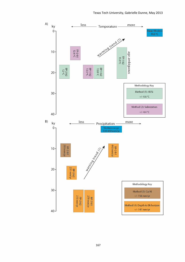
Texas Tech University, Gabrielle Dunne, May 2013
167

Texas Tech University, Gabrielle Dunne, May 2013
168
Chapter 6Summary and Conclusions
This study applies well-established methods in geochemistry to assess
the applicability on the Southern High Plains in order to produce an estimate
of climate over the last 40,000 years.
Four cores were taken from two playa basins on the Southern High
Plains, Texas. Within each core three to four soil profiles were observed.
Geochemical analysis and analysis of the physical properties of the soils
correlate well and revealed that significant weathering of the buried soil
profiles has occurred in a climate that was more arid than present. Equations
were applied to assess past MAP and MAT. Climo-functions suggest;
Temperature has increased by 5°C from bottom of the core to top.
Precipitation increased by approximately 100-150 mm/yr from bottom of the
core to top.
Analysis of the grain size distribution within the soil profile allowed for
the development of an age model based on the well known northerly fining
trend of the Blackwater Draw formation. The observed deviation from this
trend suggests that sediments have been reworked, thus an age younger than
the Blackwater Draw (~40 Ky) is inferred. A comparative age control was also
carried out using 14C dates from playas studied by Holliday et al. (2008), these
yielded dates of 21,360 14C yrs BP for soil b2 in Bailey Playa and 11,547
21,360 14C yrs BP for soil b1 in Floyd Playa.

Texas Tech University, Gabrielle Dunne, May 2013
169
The MAT and MAP were combined with the age model to suggest that
climate became warmer and wetter towards present. Thus, this study
suggests that temperature and precipitation both increased during soil forming
events by 5°C and 100-150 mm/yr, respectively, over the last 30-40 ky. This
trend is concurrent with several other studies. It can therefore be assumed
that this method of paleoclimate analysis can successfully be applied to playa
wetlands in order to produce a relatively high resolution climatic record.
Texas Tech University, Gabrielle Dunne, May 2013
170
References
Baker, C. L., 1915, Geology and underground waters of the northern Llano Estacado: Austin, University of Texas Bulletin 57, 225
Barchardt G., and Lienkaemper, J. J.,1999, Pedogenic calcite as evidence for an early Holocene dry period in the San Francisco Bay area, California. GSA Bulletin, 111, 906-918;
Barnosky, C. W., P. M. Anderson, and P. J. Bartlein, 1987, The northwestern U.S. during deglaciation: Vegetational history and paleoclimatic implications. In Wright, H. E., and W. Ruddiman (eds.), North America and Adjacent Oceans During the Last Deglaciation, The Geology of North America, Geological Society of America, 3, 289-321.
Berner, R.A., Kothavala, X., 2001. GEOCARBIII: a revised model of atmospheric CO2 over Phanerozoic time. American Journal of Science 301, 182–204
Bowen, M. W., Johnson, W. C., 2012, Late Quaternary environmental reconstructions of playa-lunette system evolution on the central High Plains of Kansas, United States, Geological Society of America Bulletin, 124, 146-161.
Bolen, E. G., L. M. Smith, and H. L. Schramm, Jr. 1989. Playalakes: prairie wetlands of the Southern High Plains, BioScience, 39, 615-623.
G.Boyle, E.A., 1983, Chemical accumulation variations under the Peru current during the past 130,000 years: Journal of Geophysical Research, 88, 7667-7680.
Brady N., and Weil R.,, 2008, The Nature and Properties of Soils, 14th Edition, Prentice Hall, Upper Saddle River, New Jersey.
Brady N., and Weil R., 2002 , The Nature and Properties of Soils, 13th Edition, Prentice Hall, Upper Saddle River, New Jersey, p/ 960.

Texas Tech University, Gabrielle Dunne, May 2013
171
Brady, Nyle. The Nature & Properties of Soils. MacMillian Publishing Company, New York: 1984
Cerling, T.E., 1984. The stable isotopic composition of modern soil carbonate and its
relationship to climate. Earth and Planetary Science Letters 71, 229–240
Chadwick, O.A., Brimhall, G.H., Hendricks, D.M., 1990. From a black to a gray box — a mass balance interpretation of pedogenesis. Geomorphology 3, 369–390.
Chepil,W. S., and Woodruff, N. P., 1963, The physics of wind erosion and its control, Advances in Agronomy, 15, 211–302.
Daniels, R.B., Gable, E.E. and Cady, I.G., 1971. The relation between geomorphology and soil morphology and genesis. Adv. Agron., 23: 51-88
Darton, N. H., 1905, Preliminary report on the geology and underground water resources of the central Great Plains: U.S. Geol. Survey Prof. 32, 433
Driese, S. G., Nordt, L. C., Warren, L. C., Stiles, C. A., Mora, C. I. and Wilding L. P., 2005, Distinguishing climate in the soil record using chemical trends in Vertisol climosequence from the Texas coast prairie and application to interesting Paleozoic paleosols in the Appalachian Basin U.S.A., Journal of sedimentary Research, 75, 339-349.
Evans, G. L., and Meade, G. E., 1945, Quaternary of the Texas High Plains, Austin, University of Texas Publication, 4401, 485–507
Feng S., Oglesby R., Rowe C. M., Loope D. B., Hu Q., 2008. Atlantic and Pacific SST influences on medieval drought in North America simulated by the Community Atmospheric Model. Journal of Geophysical research 113: 1-14.
Fox, D. L. and Koch, P. L., 2003, Tertiary history of C4 biomass in the Great Plains, USA Geology, 31, 809-812.

Texas Tech University, Gabrielle Dunne, May 2013
172
Fritz, S. C., Metcalfe, S. E., and Fritz W. D., 2001, In: Markgraf V., Iinterhemispheric Climate Linkages, Academic press, San Diego, p 241-248
Fryar, A. E., Mullican , W. and Macko, S. A., 2001,Groundwater recharge and chemical evolution in the southern High Plains of Texas, USA, Hydrogeology Journal, 9, 522–542
Gardiner D. T. and Miller R. W., 2004 Soils in our environment, 10th edition, Pearson Education, Inc, Upper Saddle River, New Jersey, p/ 641
Gilbert, G. K., 1895, Lake basins created by wind erosion, Journal of Geology, 3, 47–49
Gile, L.H., Peterson, F.F., Grossman, R.B., 1966. Morphological and genetic sequences of carbonate accumulation in desert soils. Soil Science 101, 347–360.
Golden, D.C., Chen, C.C., Dixon, J.B., and Tokashiki, Y., 1988, Pseudomorphic replacement of manganese oxides by iron oxide minerals: Geoderma, 42, 199–211
Gould, C. N., 1907, The geology and water resources of the western portion of the Panhandle of Texas: U.S. Geological Survey Water-Supply Paper 191, 70.
Graham, N. E., et al. (2007), Tropical Pacific—Mid-latitude teleconnections in medieval times, Climate Change, 83, 241 – 285,
Gustavson, T.C., and D.A. Winkler. 1988. Depositional facies of the Miocene‐Pliocene Ogallala formation, northwestern Texas and eastern New Mexico; Geology. 16: 203‐206
Gustavson, T. C., and Finley, R. C., 1985, Late Cenozoic geomorphic evolution of the Texas Panhandle and northeastern New Mexico: Austin, University of Texas Bureau of Economic Geology Report of Investigations 148, 42

Texas Tech University, Gabrielle Dunne, May 2013
173
Gustavson, T. C., Finley, R. J., and McGillis, K. A., 1980, Regional distribution of Permian salt in the Anadarko, Dalhart, and Palo Duro basins of the Texas Panhandle: Austin, University of Texas Bureau of Economic Geology Report of Investigations,106, 40.
Hall S. A., 2001, Geochronology and paleoenvironments of the glacial-age Tahoka Formation, Texas and New Mexico High Plains, New Mexico Geology, 71-77.
Hawley, J. W., Bachman, G. O., and Manley, K., 1976, Quaternary stratigraphy in the basin and range and great Basin provinces, New Mexico and western Texas. In Quaternary Stratigraphy of North America, ed. Mahaney, W. C., 235-247, Stroudburg, Pensylvania: Dowden, Hutchinson and Ross Inc.
Hills, E. S., 1940, The lunette, a new land form of aeolian origin. Australian
Geography, 3, 15–21.
Holliday, V.T., Mayer, J.H., and Fredlund, G.G., 2008, Late Quaternary sedimentology and geochronology of small playas on the southern High Plains, Texas and New Mexico, U.S.A.: Quaternary Research, 70, 11–25
Holliday, V.T., 1997, Origin and evolution of lunettes on the High Plains of Texas and New Mexico. Quaternary Research, 47, 54–69.
Holliday, V.T., Hovorka, S.D., and Gustavson, T.C., 1996, Lithostratigraphy and geochronology of fills in small playa basins on the southern High Plains, United States: Geological Society of America Bulletin, 108,953–965
Holliday, V. T. (1990). Soils and landscape evolution of eolian plains: The Southern High Plains of Texas and New Mexico. In ‘‘Soils and Landscape Evolution’’ (P. L. K. Knuepfer and L. D. McFadden, Eds.), Geomorphology, 3, 489–515.

Texas Tech University, Gabrielle Dunne, May 2013
174
Holliday, V.T., 1989, The Blackwater Draw Formation (Quaternary)—A 1.4-plus m.y. record of eolian sedimentation and soil formation on the southern High Plains: Geological Society of America Bulletin, 101, 1598–1607
Jenny, H.J., Leonard, C.D., 193, Functional relationships between soil properties and rainfall. Soil Science, 38, 363–381.
Johnson, W.C., Willey, K.L., Mason, J.A., and May, D.W., 2007, Stratigraphy and environmental reconstruction at the Middle Wisconsinan Gilman Canyon Formation type locality, Buzzard’s Roost, southwestern Nebraska USA: Quaternary Research, 67, 474–486,
Johnson E., 2007, Grassland Ecosystems of the Llano Estacado In: Sosebee, R.E.; Wester, D.B.; Britton, C.M.; McArthur, E.D.; Kitchen, S.G., comp. 2007. Proceedings: Shrubland dynamics—fire and water; 2004 August 10-12; Lubbock, TX. Proceedings RMRS-P-47. Fort Collins, CO: U.S. Department of Agriculture, Forest Service,Rocky Mountain Research Station. 173.
Johnson,W. D., 1901, The High Plains and their utilization: U.S. Geological Survey 21st Annual Report for 1899–1900, pt. IV, 601–741.
Judson, S., 1950, Depressions of the northern portion of the Southern High Plains of eastern New Mexico, Geological Society of America Bulletin, 61, 253–274.
Judson, S., 1953, Geology of the San Jon site, eastern New Mexico: Smithsonian Miscellaneous Collections, 121, 70.
Kaczorowski, R. T., 1977, The Carolina Bays: A comparison with modern oriented lakes: Columbia, University of South Carolina Department of Geology, Coastal Research Division Technical Report no. 13-CRD, 124 p.
Kahmann, J. A., & Driese, S. G. 2008. Paleopedology and geochemistry of Late Mississippian (Chesterian) Pennington Formation paleosols at Pound Gap, Kentucky, USA: Implications for high-frequency climate variations. Palaeogeography, Palaeoclimatology, Palaeoecology, 259, 357-381.

Texas Tech University, Gabrielle Dunne, May 2013
175
Laird, K. R., Cumming, B. F., Wunsam, S., Rusak, J., Oglesby, R. J., Fritz, S. C. Leavitt, P. R. 2003. Lake sediments record large-scale shifts in moisture regimes across the northern prairies of North America during the past two millennia. Proc. Natl. Acad. Sci. 100, 2483–2488
Lang, W. B., 1938, Geology of the Pecos River between Laguna Grande de la Sal and Pierce Canyon: New Mexico State Engineer 12th and 13th Bien. Repts., p. 80-86
Lotspeich, F. B.,& Everhart, M. E., 1962,Climate and Vegetation as Soil Forming Factors on the Llano Estacado, Journal of Range Management, 15, 134-141.
MacDonald, G.M., Kremenetski, K.V. Hidalgo, H. 2008. Southern California and the Perfect Drought: simultaneous prolonged drought in Southern California and the Sacramento and Colorado River systems. Quaternary International 188, 11-23.
Mack, G. H., 2003, Lower Permian terrestrial paleoclimate indicators in New mexico and their comparison to paleoclimate models. New Mexico Geological Society Guidebook, 54, 231-240
Netthisinghe, A.., 2008, surface and subsurface flow relationships to Ogalalla Aquifer recharge on the Southern High Plains of Texas, Texas Tech University. Thesis.
Nordt, L., Von Fischer, J, and Tieszen, L., 2007 Late Quaternary temperature record from buried soils of the North American Great Plains, Geology, 35, 159–162
Osterkamp W.R. and Wood W.W, 1987a, Playa-lake basins on the Southern High Plains of Texas and New Mexico: Part I Hydrologic, geomorphic, and geologic evidence for their development, Geol. Soc. Am. Bull., 99 215–223

Texas Tech University, Gabrielle Dunne, May 2013
176
Osterkamp W.R. and Wood W.W, 1987b, Playa-lake basins on the Southern High Plains of Texas and New Mexico: Part II. A hydrologic model and mass-balance arguments for their development, Geol. Soc. Am. Bull., 99, 224-230.
Paine, J. G., 1994, Subsidence beneath a playa basin on the Southern High Plains U.S.A.: Evidence from shallow seismic data: Geological Society of America Bulletin, 106, 233–242.
Patton, L. T., 1935, Some observations on the so-called “lakes” of the Llano Estacado of Texas, Geological Society of America Proceedings, p. 451.
Porter S., 1989, Some Geological Implications of Average Quaternary Glacial Conditions, Quaternary Research, 32, 245-261
Price, W. A., 1944, Greater American deserts: Texas Academy of Sciences,
Proceedings and Transactions, 27, 163–170.
Reeves, C. C., Jr., 1990, A proposed sequential development of lake basins, Southern High Plains, Texas and New Mexico, in Gustavson, T. C., ed., Geologic framework and regional hydrology: Upper Cenozoic Blackwater Draw and Ogallala Formations, Great Plains: Austin, University of Texas Bureau of Economic Geology, p. 209–232.
Reeves, C. C., Jr., and Temple, J. M., 1986, Permian salt dissolution, alkaline lake basins, and nuclear waste storage, Southern High Plains, Texas and New Mexico: Geology, 14, 939–942
.Reeves, C.C., Jr., 1976, Tertiary-Quaternary stratigraphy and geomorphology of west Texas and south-eastern New Mexico, in Kelley, V., and Trauger, F.D., eds., Guidebook for east-central New Mexico: New Mexico Geological Society Guidebook 24, 108–117
Reeves, C. C., Jr., 1972, Tertiary–Quaternary stratigraphy and geomorphology of west Texas and southeastern New Mexico, in Kelly, V. C., and Trauger, F. D., eds., Guidebook to east-central New Mexico: Socorro, New Mexico Geological Society, p. 108–117.
Texas Tech University, Gabrielle Dunne, May 2013
177
Reeves, C. C., Jr., 1971, Relations of caliche to small natural depressions, Southern High Plains, Texas and New Mexico: Geological Society of America Bulletin, 82, 1983–1988.
Reeves, C. C., Jr., 1966, Pluvial lake basins of West Texas: Journal of Geology, 74, 269–291
Retallack, G.J., 2007, Cenozoic Paleoclimate on Land in North America The Journal of Geology, 2007, 115, 271–294]
Retallack, G.J., 2005, Pedogenic carbonate proxies for amount and seasonality of precipitation in paleosols: Geology, 33, 333–336.
Retallack, G.J., 2001. Soils of the past. Blackwell, Oxford.
Retallack, G.J., 2000. Depth to pedogenic carbonate horizon as a paleoprecipitation indicator? comment and reply. Geology 28, 572–573.
Retallack, G. J., 1997, A Colour Guide to Paleosols, John Wiley & Sons Ltd, Chichester, England.
Retallack, G.J., 1991. Untangling the effects of burial alteration and ancient soil formation. Annual Review of Earth Planetary Sciences 19, 183–206.
Retallack , G. J, 1990, Soils of the Past: An Introduction to Paleopedology, Unwin Hyman , inc. Mass.
Royer, D.L.,1999, Depth to pedogenic carbonate horizon as a paleoprecipitation indicator. Geology, 27, 1123-1126.
Russell, R. J. 1945. Climates of Texas. Ann. Assoc. Amer. Geographers, 35, 37-52.
Sabin, T.J., and Holliday, V.T., 1995, Playas and lunettes on the southern High Plains: Morphometric and spatial relationships: Annals of the Association of American Geographers, 85, 286–305

Texas Tech University, Gabrielle Dunne, May 2013
178
Sehgal, J.L., and Stoops, G., 1972, Pedogenic calcite accumulation in arid and semi-arid regions of the Indo-Gangetic alluvial plain of erstwhile Punjab (India)—Their morphologyand origin: Geoderma, 8, 59–72.
Sheldon, N. D. and Tabor, N. J., 2009, Quantitative paleoenvironmental and paleoclimatic reconstruction using paleosols, Earth-Science Reviews , 95,1–52
Sheldon N. D., Retallack, G. J., Tanaka, S.,, 2002, Geochemical climofunctions from North American Soils and Applications to paleosols across the Eocene-Oligocene boundary in Oregon, Geology, 110, 687-696
Sheldon, N.D., 2006a. Abrupt chemical weathering increase across the Permian–Triassic boundary. Palaeogeography, Palaeoclimatology, Palaeoecology 231, 315–321
Sheldon, N.D., 2006b. Quaternary glacial–interglacial climate cycles in Hawaii. Journal of Geology, 114, 367–376.
Smith, L. M., 2003, Playas of The Great Plains; Austin, Texas, University of Texas Press, p. 257.
Stiles C. A., Mora, C. L. and Driese S. G., 2003, pedogenic processes and domain boundaries in a Vertisol climosequence: evidence from titanium and zirconium distribution and morphology Geoderma 116, 279–299.
Stiles C. A., Mora, C. L. and Driese S. G., 2001 Pedogenic iron-manganese nodules in Vertisols: A new proxy for paleoprecipitation? Geology, 29, 943–946
Stine, S., 1994: Extreme and persistent drought in California and Patagonia during medieval time. Nature, 369: 546-549.
Stone, W. J., 1990. Natural recharge of the Ogallala aquifer through playas and other non-stream-channel settings, eastern New Mexico. In: Gustavson, T.C., eds., Geologic framework and regional hydrology: upper Cenozoic
Texas Tech University, Gabrielle Dunne, May 2013
179
Blackwater Draw and Ogallala Formations, Great Plains. Univ. Texas Austin, Bur. Econ. Geol., pp. 180-192
Tabor N. J., Montanez, I. P., Scotese, C. R., Poulsen, C. J. Mack, G. H., 2008, Palesol archives of environmental and climatic history in paleotroical western Pangea during the latest Pennsylvanian through early Permian, The Geological society of America Special Paper, 441, 291-303.
Tabor N. J., and Montanez, I. P, 2004, Permo-Pennsylvanian alluvial paleosols (north-central Texas): High resolution proxy records of the evolution of the early Pangean Palaeoclimate: Sedimentology, 51, 851-884.
Tabor, N.J., Montañez, I.P., 2002. Shifts in late Paleozoic atmospheric circulation over western equatorial Pangea: insights from pedogenic mineral δ18O compositions. Geology, 30, 1127–1130.
Van Devender, T. R., R. S. Thompson, and J. L. Betancourt, 1987: Vegetation history of the deserts of southwestern North America: The nature and timing of the Late Wisconsin-Holocene transition. In Ruddiman, W., and H. E. Wright (eds.), North America and Adjacent Oceans During the Last Deglaciation. Boulder, Geological Society of America, 323-352..
Wilkins, G. R., P. A. Delcourt, H. R. Delcourt, F. W. Harrison, and M. R. Turner, 1991, Paleoecology of central Kentucky since the Last Glacial Maximum. Quaternary Research, 36, 224-239.
Wood W. W., 2002 Role of Groundwater in Geomorphology, Geology and Paleoclimate of the Southern Great Plains, Groundwater, 40, 438-447.
Wood, W. W., and Osterkamp, W. R., 1984, Playa lake basins on the Southern High Plains of Texas, U.S.A.: A hypothesis for their development: Lubbock, Texas Tech University Water Resources Center, Ogallala Aquifer Symposium II Proceedings, p. 304–311

Texas Tech University, Gabrielle Dunne, May 2013
180
.Woodhouse, C.A., and Overpeck, J.T., 1998, 2000 years of drought variability in the central United States: Bulletin of the American Meteorological Society, 79, 2693–2714.
Woodhouse CA, Meko DM, MacDonald GM, Stahle DW, Cook ER , 2010, A 1,200-year perspective of 21st century drought in southwestern North America. Proc Natl Acad Sci USA 107:21283–21288.
Worster, D., 1979, Dust Bowl: The Southern Plains in the 1930s: New York, Oxford University Press, 277.

Texas Tech University, Gabrielle Dunne, May 2013
181
Appendix
Loss On Ignition Data BP-1
Sample # Crucible Number
Crucible Weight (g)
Cruc.+ Wet Wt.
(g)
Cruc. + Fused Wt. (g)
LOI
BP1 - 0 1.00 8.84 10.84 10.71 6.46
BP1- 10 2.00 7.84 9.79 9.66 6.28
BP1 - 20 3.00 7.81 9.84 9.74 4.49
BP1- 30 4.00 8.08 10.18 10.08 4.97
BP1- 40 5.00 8.25 10.26 10.15 5.18
BP1 - 50 6.00 7.76 9.74 9.63 5.76
BP1-60 1.00 9.69 11.62 11.50 5.86
BP1-70 2.00 8.93 10.90 10.77 6.77
BP1-80 3.00 8.41 10.41 10.27 6.90
BP1-90 4.00 9.28 11.21 11.05 7.84
BP1-100 5.00 8.12 10.18 10.01 8.30
BP1-110 6.00 8.66 10.68 10.51 8.20
BP1-120 1.00 9.69 11.63 11.46 8.65
BP1-130 2.00 8.93 10.95 10.76 9.34
BP1-140 3.00 9.28 11.26 11.07 9.57
BP1-150 4.00 8.41 10.41 10.22 9.39
BP1-160 5.00 8.12 10.16 9.96 9.84
BP1-170 6.00 8.66 10.66 10.47 9.39
BP1-180 1.00 8.84 10.69 10.52 9.29
BP1-190 2.00 7.84 9.75 9.56 9.80
BP1-200 3.00 7.80 9.83 9.63 9.67
BP1-210 4.00 8.08 10.10 9.89 10.16
BP1-220 5.00 8.25 10.20 10.00 10.62
BP1-230 6.00 7.76 9.77 9.57 10.19
BP1-240 1.00 7.84 9.77 9.57 10.22
BP1-250 2.00 7.76 9.79 9.58 10.20
BP-260 1.00 9.69 11.42 11.24 10.32
BP-270 2.00 8.93 10.59 10.42 10.35
BP1-280 3.00 9.28 11.27 11.07 10.30
BP1-290 4.00 8.66 10.63 10.42 10.72
BP1-300 5.00 8.41 10.42 10.21 10.57
BP1-310 6.00 8.12 10.16 10.00 7.95
BP1-320 1.00 8.66 10.66 10.47 9.56
BP1-330 2.00 8.41 10.45 10.26 9.39
BP1-340 3.00 9.28 11.18 10.91 14.02
BP1-0 R 3.00 7.80 9.92 9.78 6.59

Texas Tech University, Gabrielle Dunne, May 2013
182
BP1-80 R 4.00 8.25 10.39 10.24 6.89
BP1-110 R 5.00 8.08 10.15 9.98 8.28
BP1-180 R 6.00 8.84 10.67 10.50 9.37
BP1-310 R 4.00 8.12 10.28 10.10 8.04
BP1-80 R 5.00 9.69 11.41 11.29 6.96
BP1-110 R 6.00 8.93 10.76 10.61 8.12
BP1-280 R 5.00 7.81 9.94 9.71 10.49
R - Repeat

Texas Tech University, Gabrielle Dunne, May 2013
183
Loss On Ignition Data BP-2
Sample # Crucible Number
Crucible Weight (g)
Cruc.+ Wet Wt.
(g)
Cruc. + Fused Wt.
(g)
LOI
BP2-0 1.00 7.80 9.86 9.61 11.98
BP2 - 10 2.00 7.84 9.79 9.56 11.97
BP2 - 20 3.00 8.25 10.12 9.91 11.27
BP2 - 30 4.00 8.84 10.81 10.61 10.11
BP2 - 40 5.00 7.76 9.73 9.51 10.86
BP2 - 50 6.00 8.08 10.06 9.84 11.35
BP2 - 60 1.00 8.41 10.34 10.12 11.42
BP2 - 70 2.00 8.93 10.84 10.64 10.50
BP2 - 80 3.00 8.12 10.10 9.90 10.52
BP2 - 90 4.00 8.66 10.43 10.25 10.24
BP2 - 100 5.00 9.28 11.04 10.91 7.05
BP2 - 110 6.00 9.69 11.62 11.49 6.89
BP2 - 120 1.00 8.12 10.13 10.00 6.51
BP2 - 130 2.00 8.93 10.90 10.77 6.31
BP2 - 140 3.00 8.66 10.56 10.42 7.42
BP2 - 150 4.00 9.69 11.52 11.37 7.95
BP2 - 160 5.00 8.41 10.45 10.30 7.57
BP2 - 170 6.00 9.29 11.47 11.30 7.77
BP2 - 180 1.00 7.76 9.85 9.69 7.70
BP2 - 190 2.00 7.80 9.91 9.72 8.96
BP2 - 200 3.00 7.84 9.72 9.57 7.82
BP2 - 210 4.00 8.08 9.82 9.68 8.28
BP2 - 220 5.00 8.84 10.44 10.30 8.89
BP2 - 230 6.00 8.25 10.30 10.09 10.45
BP2 - 240 1.00 9.29 11.09 10.90 10.49
BP2 - 250 2.00 8.41 10.20 10.02 10.40
BP2 - 260 3.00 8.93 11.03 10.87 7.56
BP2 - 270 4.00 8.66 10.62 10.46 8.01
BP2 - 280 5.00 9.69 11.52 11.37 8.07
BP2 - 290 6.00 8.12 10.25 10.07 8.19
BP2 - 300 1.00 7.84 9.80 9.63 8.49
BP2 - 310 2.00 8.25 10.16 9.99 8.78
BP2 - 320 3.00 8.08 10.01 9.85 8.67
BP2 - 330 4.00 7.77 9.83 9.63 9.39
BP2-0 R 1.00 9.28 11.18 10.95 12.07
BP2-110 R 6.00 8.84 10.87 10.73 6.89
BP2-130 R 2.00 8.41 10.32 10.20 6.33
BP - 300 R 3.00 8.93 10.98 10.81 8.54
BP2-200 R 4.00 8.66 10.55 10.40 7.68
BP2-130 R 5.00 9.69 11.44 11.33 6.36
BP2-300 R 6.00 8.12 9.99 9.83 8.56

Texas Tech University, Gabrielle Dunne, May 2013
184
Loss On Ignition Data FP-1
Sample # Crucible Number
Crucible Weight (g)
Cruc.+ Wet Wt. (g)
Cruc. + Fused Wt.
(g)
LOI
FP1 - 0 1.00 9.29 11.22 11.00 11.44
FP1- 10 2.00 8.66 10.75 10.52 11.32
FP1 - 20 3.00 8.41 10.48 10.25 11.45
FP1 - 30 4.00 8.93 10.95 10.72 11.53
FP1- 40 5.00 8.12 10.14 9.91 11.79
FP1 - 50 6.00 9.69 11.72 11.49 11.45
FP1 - 60 1.00 7.80 9.86 9.62 11.72
FP1- 70 2.00 7.84 9.88 9.65 11.41
FP1 - 80 3.00 8.25 10.61 10.33 12.02
FP1 - 120 4.00 8.84 10.98 10.67 11.47
FP1- 130 5.00 8.08 10.17 9.93 11.29
FP1 - 140 6.00 7.76 9.95 9.70 11.45
FP1 - 150 1.00 8.93 10.94 10.71 11.42
FP1- 160 2.00 9.69 11.60 11.38 11.55
FP1 - 170 3.00 8.12 10.14 9.90 11.66
FP1 - 180 4.00 8.66 10.61 10.38 11.61
FP1- 190 5.00 8.41 10.47 10.19 11. 71
FP1 - 200 6.00 9.28 11.46 11.21 11.78
FP1 - 210 1.00 7.84 9.89 9.64 11.83
FP1- 220 2.00 7.80 9.91 9.65 12.56
FP1 - 230 3.00 8.84 10.83 10.59 12.31
FP1 - 240 4.00 7.76 9.71 9.47 12.29
FP1 - 250 5.00 8.25 10.25 10.00 12.65
FP1- 260 6.00 8.08 10.01 9.78 12.14
FP1 - 270 1.00 7.84 9.81 9.55 13.40
FP1 - 280 2.00 7.76 9.75 9.49 13.26
FP1 - 290 3.00 8.08 10.20 9.91 13.25
FP1 - 300 4.00 7.80 9.83 9.57 13.12
FP1 - 310 5.00 8.84 10.92 10.64 13.19
FP1 - 320 6.00 8.26 10.48 10.19 12.75

Texas Tech University, Gabrielle Dunne, May 2013
185
Loss On Ignition Data FP-2
Sample # Crucible Number
Crucible Weight (g)
Cruc.+ Wet Wt. (g)
Cruc. + Fused Wt. (g)
LOI
FP2 - 0 1.00 7.77 9.71 9.51 10.23
FP2 - 10 2.00 8.08 10.02 9.82 9.98
FP2 - 20 3.00 7.80 9.77 9.58 9.64
FP2 - 30 4.00 7.85 9.85 9.65 10.22
FP2 - 40 5.00 8.25 10.31 10.10 10.19
FP2 - 50 6.00 8.84 10.86 10.66 10.03
FP2 - 60 1.00 9.70 11.62 11.36 13.49
FP2 - 70 2.00 9.28 11.31 11.12 9.74
FP2 - 80 3.00 8.41 10.44 10.27 8.78
FP2 - 90 4.00 8.93 10.94 10.77 8.57
FP2 - 100 5.00 8.12 10.17 10.09 4.00
FP2 - 110 6.00 8.66 10.64 10.57 3.44
FP2 - 120 1.00 8.83 10.93 10.83 4.62
FP2 - 130 2.00 8.25 10.32 10.22 4.68
FP2 - 140 3.00 7.84 9.83 9.78 2.52
FP2 - 150 4.00 7.80 9.93 9.87 2.80
FP2 - 160 5.00 8.08 10.06 9.93 6.72
FP2 - 170 6.00 7.76 9.98 9.72 12.11
FP2 - 180 1.00 9.69 11.64 11.53 5.72
FP2 - 190 2.00 8.41 10.71 10.60 4.55
FP2 - 200 3.00 8.93 10.96 10.86 5.04
FP2 - 210 4.00 9.28 11.28 11.16 5.58
FP2 - 220 5.00 8.66 10.63 10.52 5.33
FP2 - 230 6.00 8.12 10.42 10.29 5.53
FP2 - 240 1.00 8.83 10.79 10.68 5.87
FP2 - 250 2.00 8.25 10.35 10.22 6.33
FP2 - 260 3.00 7.76 9.94 9.79 6.61
FP2 - 270 4.00 7.80 9.93 9.79 6.57
FP2 - 280 5.00 7.84 9.81 9.67 6.92
FP2 - 290 6.00 8.08 10.02 9.89 6.42
FP2 - 300 1.00 8.12 10.16 10.02 6.58
FP2 - 310 2.00 8.93 10.72 10.59 7.42
FP2 - 320 3.00 8.66 10.59 10.45 6.92
FP2 - 330 4.00 9.28 11.22 11.07 7.63
FP2 - 340 5.00 9.69 11.64 11.48 8.38