Embed Size (px)
Citation preview

Copyright 2006 McGraw-Hill Australia Pty Ltd PPTs t/a Macroeconomics 2e by Dornbusch, Bodman, Crosby, Fischer, StartzSlides prepared by Dr Monica Keneley.
12-1
Chapter 12Consumption and Saving
Copyright 2006 McGraw-Hill Australia Pty Ltd PPTs t/a Macroeconomics 2e by Dornbusch, Bodman, Crosby, Fischer, StartzSlides prepared by Dr Monica Keneley.
12-2
Objectives
• Evaluate modern theories of consumption which link lifetime consumption to lifetime income
• Consider consumption under uncertainty
• Investigate further aspects of consumption behaviour
• Explain the Barro-Ricardo problem
Copyright 2006 McGraw-Hill Australia Pty Ltd PPTs t/a Macroeconomics 2e by Dornbusch, Bodman, Crosby, Fischer, StartzSlides prepared by Dr Monica Keneley.
12-3
Chapter Organisation
12.1 The Life-Cycle–Permanent-Income Theory of Consumption and Saving
12.2 Consumption under Uncertainty: the Modern Approach
12.3 Further Aspects of Consumption Behaviour

Copyright 2006 McGraw-Hill Australia Pty Ltd PPTs t/a Macroeconomics 2e by Dornbusch, Bodman, Crosby, Fischer, StartzSlides prepared by Dr Monica Keneley.
12-4
12.1 Consumption and Saving
• Consumption accounts for more than 61% of aggregate demand.
• A simple model of consumption was outlined in Chapter 7.
• It assumed that consumption was determined by disposable income in a simple linear relation.
(12.1)
Copyright 2006 McGraw-Hill Australia Pty Ltd PPTs t/a Macroeconomics 2e by Dornbusch, Bodman, Crosby, Fischer, StartzSlides prepared by Dr Monica Keneley.
12-5
12.1 The Life-Cycle Theory
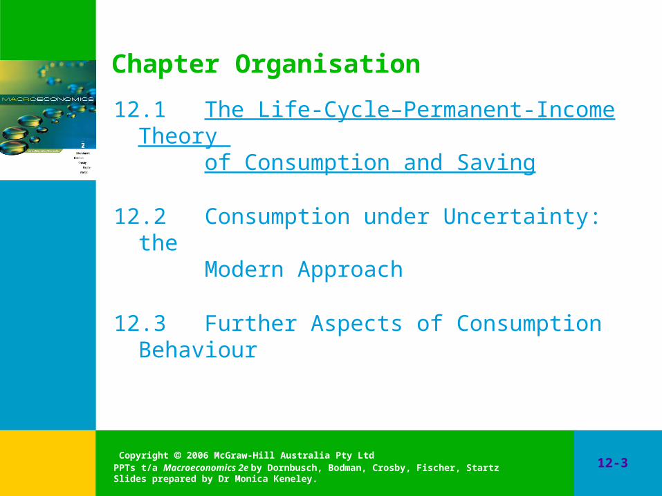
• Life-cycle (LC) hypothesis– Individuals plan their consumption and savings
behaviour over long periods with the intention of allocating consumption over their entire lifetime.
• A key assumption is individuals choose to consume at about the same level every period.
• This implies that the MPC will vary over the life-cycle of the individual.
Copyright 2006 McGraw-Hill Australia Pty Ltd PPTs t/a Macroeconomics 2e by Dornbusch, Bodman, Crosby, Fischer, StartzSlides prepared by Dr Monica Keneley.
12-6
The Life-Cycle Theory
• Modern consumption theories consider the way in which individuals plan and make choices over an extended period of time.
• Two theories explain consumption patterns:– The life-cycle hypothesis– The permanent income theory.
• These two models focus on different aspects of consumption planning.
• Today, these two theories have largely merged.

Copyright 2006 McGraw-Hill Australia Pty Ltd PPTs t/a Macroeconomics 2e by Dornbusch, Bodman, Crosby, Fischer, StartzSlides prepared by Dr Monica Keneley.
12-7
The Life-Cycle Theory
• Example– Assume a person starts work at 20, plans to work
until they are 65, expects to die at 80, and earns – $30 000 a year (YL).– The person’s lifetime resources would be YL times
working life (WL) or $30 000 (65 – 20) = $1.35m.– Spreading the lifetime resources over the lifespan (NL)
gives an annual C of $22 500.– C = (WL/NL) YL = $1.35m/(80 – 20) = $22 500

Copyright 2006 McGraw-Hill Australia Pty Ltd PPTs t/a Macroeconomics 2e by Dornbusch, Bodman, Crosby, Fischer, StartzSlides prepared by Dr Monica Keneley.
12-8
The Life-Cycle Theory
• Example– C = (WL/NL) YL– So the MPC is WL/NL = (65 – 20)/(80 – 20) = 0.75
• Consider now a permanent increase in Y of $3000:– The extra Y times 45 working years spread over 60 years
of life would increase annual consumption by +$3000 (45/60) = +$2250
– The MPC out of permanent Y would still be: WL/NL = 45/60 = 0.75
Copyright 2006 McGraw-Hill Australia Pty Ltd PPTs t/a Macroeconomics 2e by Dornbusch, Bodman, Crosby, Fischer, StartzSlides prepared by Dr Monica Keneley.
12-9
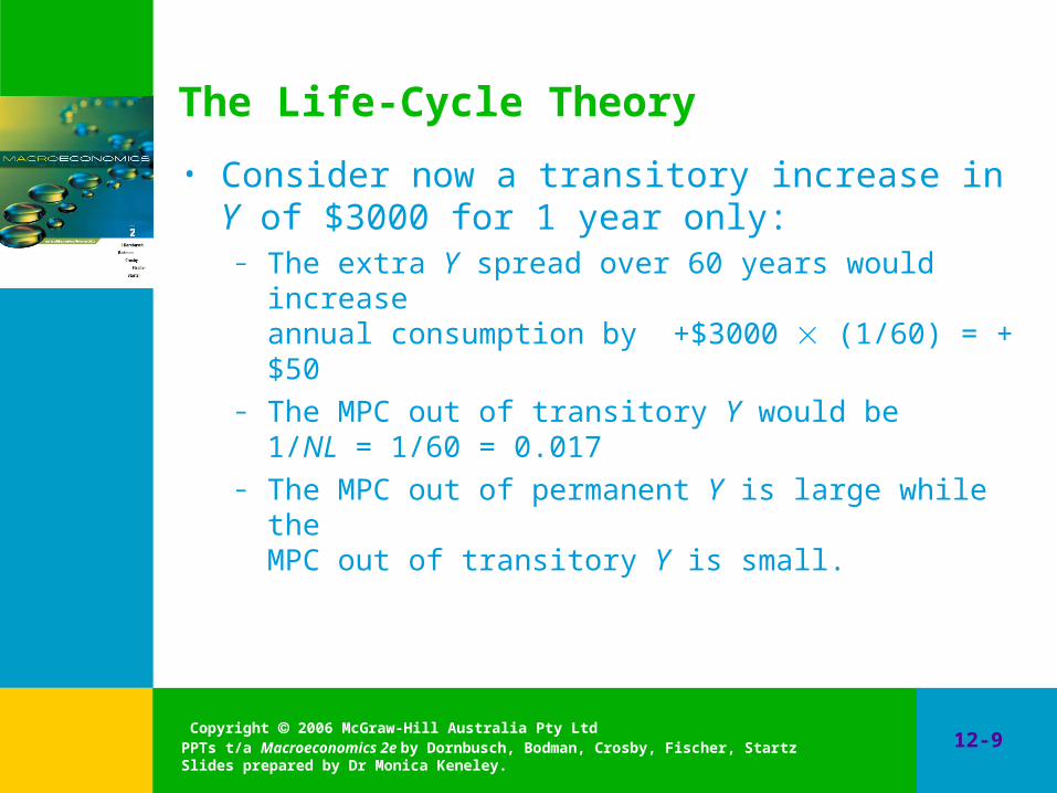
The Life-Cycle Theory
• Consider now a transitory increase in Y of $3000 for 1 year only:
– The extra Y spread over 60 years would increase annual consumption by +$3000 (1/60) = +$50
– The MPC out of transitory Y would be 1/NL = 1/60 = 0.017
– The MPC out of permanent Y is large while the MPC out of transitory Y is small.
Copyright 2006 McGraw-Hill Australia Pty Ltd PPTs t/a Macroeconomics 2e by Dornbusch, Bodman, Crosby, Fischer, StartzSlides prepared by Dr Monica Keneley.
12-10
Permanent-Income Theory
• The Permanent-Income hypothesis (PIH) claims C is not related to current Y but rather longer-term estimates of Y.
• Permanent-Income is:– The steady rate of C a person could maintain for the
rest of his or her life– Given the present level of wealth and the Y earned
now and in the future.
Copyright 2006 McGraw-Hill Australia Pty Ltd PPTs t/a Macroeconomics 2e by Dornbusch, Bodman, Crosby, Fischer, StartzSlides prepared by Dr Monica Keneley.
12-11
Permanent-Income Theory
• This implies that consumption is proportional to permanent Y.
• C = cYP (12.2)
• Where YP is permanent (disposable) Y.
• Transitory Y is assumed not to have any substantial affects on consumption.
Copyright 2006 McGraw-Hill Australia Pty Ltd PPTs t/a Macroeconomics 2e by Dornbusch, Bodman, Crosby, Fischer, StartzSlides prepared by Dr Monica Keneley.
12-12
Chapter Organisation
12.1 The Life-Cycle–Permanent-Income Theory of Consumption and Saving
12.2 Consumption under Uncertainty: the Modern Approach
12.3 Further Aspects of Consumption Behaviour
Copyright 2006 McGraw-Hill Australia Pty Ltd PPTs t/a Macroeconomics 2e by Dornbusch, Bodman, Crosby, Fischer, StartzSlides prepared by Dr Monica Keneley.
12-13
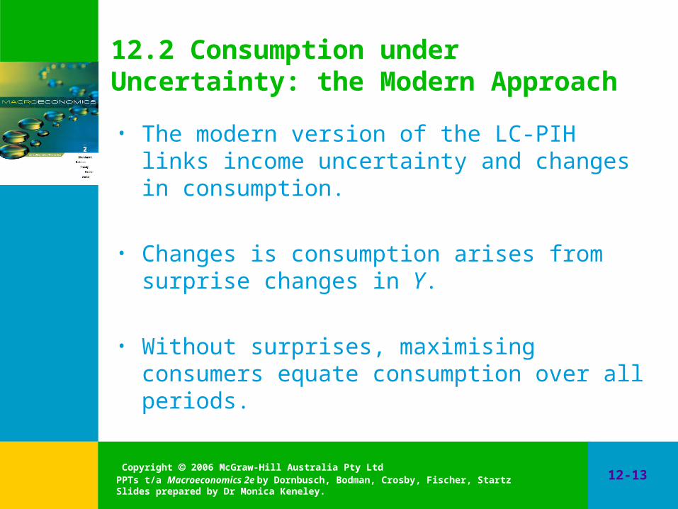
12.2 Consumption under Uncertainty: the Modern Approach
• The modern version of the LC-PIH links income uncertainty and changes in consumption.
• Changes is consumption arises from surprise changes in Y.
• Without surprises, maximising consumers equate consumption over all periods.
Copyright 2006 McGraw-Hill Australia Pty Ltd PPTs t/a Macroeconomics 2e by Dornbusch, Bodman, Crosby, Fischer, StartzSlides prepared by Dr Monica Keneley.
12-14
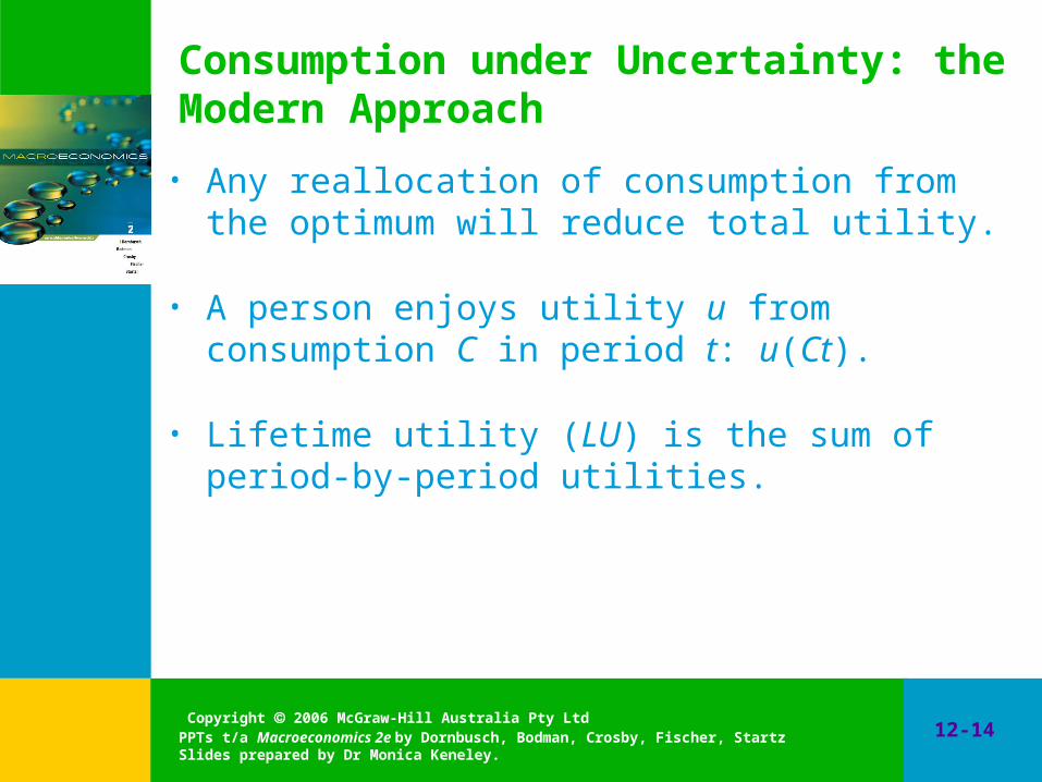
Consumption under Uncertainty: the Modern Approach
• Any reallocation of consumption from the optimum will reduce total utility.
• A person enjoys utility u from consumption C in period t: u(Ct).
• Lifetime utility (LU) is the sum of period-by-period utilities.
Copyright 2006 McGraw-Hill Australia Pty Ltd PPTs t/a Macroeconomics 2e by Dornbusch, Bodman, Crosby, Fischer, StartzSlides prepared by Dr Monica Keneley.
12-15
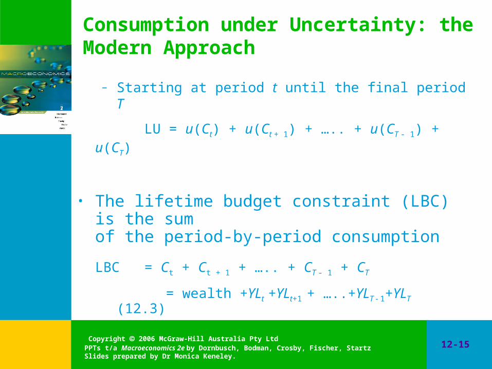
Consumption under Uncertainty: the Modern Approach
– Starting at period t until the final period T
LU = u(Ct) + u(Ct + 1) + ….. + u(CT - 1) + u(CT)
• The lifetime budget constraint (LBC) is the sum of the period-by-period consumption
LBC = Ct + Ct + 1 + ….. + CT - 1 + CT
= wealth +YLt +YLt+1 + …..+YLT - 1+YLT (12.3)

Copyright 2006 McGraw-Hill Australia Pty Ltd PPTs t/a Macroeconomics 2e by Dornbusch, Bodman, Crosby, Fischer, StartzSlides prepared by Dr Monica Keneley.
12-16
Consumption under Uncertainty: the Modern Approach
• Equation 12.3 states that consumers choose consumption each period:
– To maximise lifetime utility
– Subject to total lifetime resources.
• The optimal choice is the C path that equates the marginal utility of C across periods:
– MU(Ct + 1) = MU(Ct)
– No reallocation over time can increase total utility.
Copyright 2006 McGraw-Hill Australia Pty Ltd PPTs t/a Macroeconomics 2e by Dornbusch, Bodman, Crosby, Fischer, StartzSlides prepared by Dr Monica Keneley.
12-17
Consumption under Uncertainty: the Modern Approach
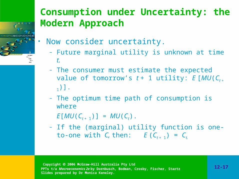
• Now consider uncertainty.– Future marginal utility is unknown at time t.– The consumer must estimate the expected value of
tomorrow’s t + 1 utility: E [MU(Ct + 1)].
– The optimum time path of consumption is where
E[MU(Ct + 1)] = MU(Ct).
– If the (marginal) utility function is one-to-one with C, then: E (Ct + 1) = Ct.

Copyright 2006 McGraw-Hill Australia Pty Ltd PPTs t/a Macroeconomics 2e by Dornbusch, Bodman, Crosby, Fischer, StartzSlides prepared by Dr Monica Keneley.
12-18
Consumption under Uncertainty: the Modern Approach
• Now consider uncertainty.– E (Ct + 1) = Ct
– If observed C is expected C with a random surprise Ct + 1 = E (Ct + 1) +
– Then substituting for the expected value derives a simple random-walk model of consumption
Ct + 1 = E (Ct + 1) +
= Ct +
Copyright 2006 McGraw-Hill Australia Pty Ltd PPTs t/a Macroeconomics 2e by Dornbusch, Bodman, Crosby, Fischer, StartzSlides prepared by Dr Monica Keneley.
12-19
Consumption under Uncertainty: the Modern Approach
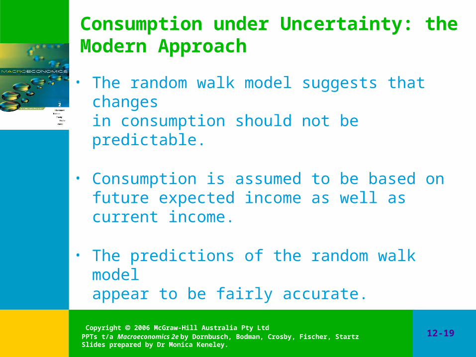
• The random walk model suggests that changes in consumption should not be predictable.
• Consumption is assumed to be based on future expected income as well as current income.
• The predictions of the random walk model appear to be fairly accurate.
Copyright 2006 McGraw-Hill Australia Pty Ltd PPTs t/a Macroeconomics 2e by Dornbusch, Bodman, Crosby, Fischer, StartzSlides prepared by Dr Monica Keneley.
12-20
LC–PIH: The Traditional Model Strikes Back
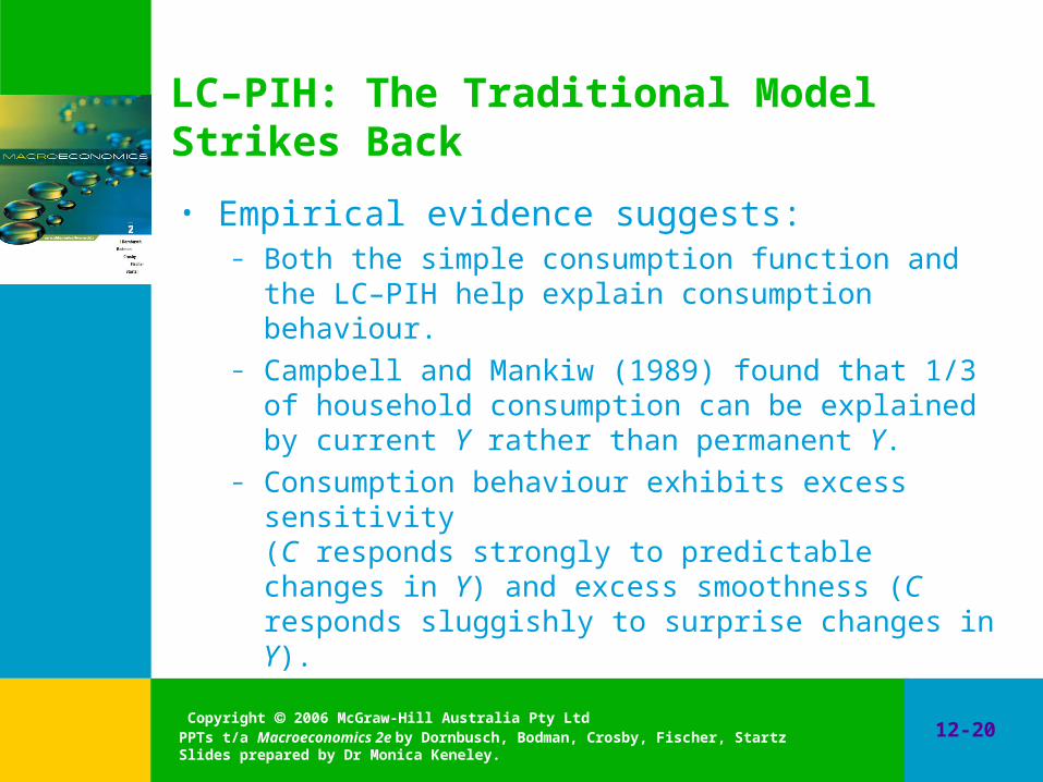
• Empirical evidence suggests:– Both the simple consumption function and the LC–PIH
help explain consumption behaviour.– Campbell and Mankiw (1989) found that 1/3 of household
consumption can be explained by current Y rather than permanent Y.
– Consumption behaviour exhibits excess sensitivity (C responds strongly to predictable changes in Y) and excess smoothness (C responds sluggishly to surprise changes in Y).
Copyright 2006 McGraw-Hill Australia Pty Ltd PPTs t/a Macroeconomics 2e by Dornbusch, Bodman, Crosby, Fischer, StartzSlides prepared by Dr Monica Keneley.
12-21
Liquidity Constraints and Myopia
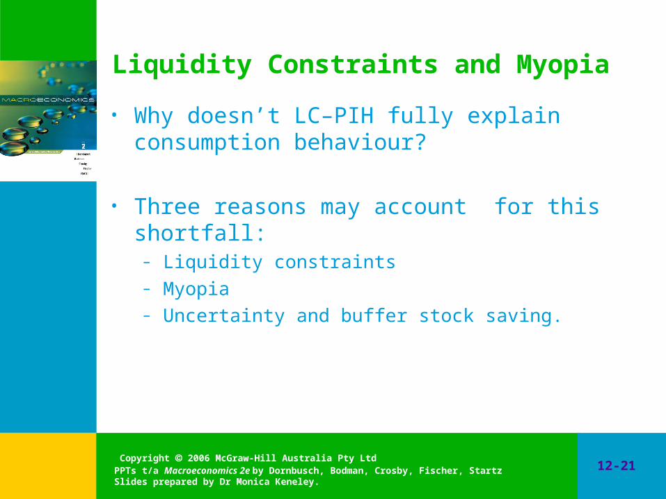
• Why doesn’t LC–PIH fully explain consumption behaviour?
• Three reasons may account for this shortfall:– Liquidity constraints– Myopia– Uncertainty and buffer stock saving.
Copyright 2006 McGraw-Hill Australia Pty Ltd PPTs t/a Macroeconomics 2e by Dornbusch, Bodman, Crosby, Fischer, StartzSlides prepared by Dr Monica Keneley.
12-22
Liquidity Constraints and Myopia
• Liquidity constraints– Represent constraints on borrowing– A consumer may not be able to borrow to sustain current
consumption in the expectation of higher future Y– Example: Students cannot obtain a large loan now
merely on the basis of expected higher future Y.
Copyright 2006 McGraw-Hill Australia Pty Ltd PPTs t/a Macroeconomics 2e by Dornbusch, Bodman, Crosby, Fischer, StartzSlides prepared by Dr Monica Keneley.
12-23
Liquidity Constraints and Myopia
• Myopia– Consumers may not be as forward looking as
suggested by the LC–PIH – They take a short-sighted approach– Example: An announcement that social security
benefits will be increased in 6 weeks' time– Doesn’t increase consumption (until benefits are
paid) because the recipients do not have the available assets to increase consumption (liquidity constraint), or
– They do not pay attention to the announcement (myopia), or they don’t believe it.
Copyright 2006 McGraw-Hill Australia Pty Ltd PPTs t/a Macroeconomics 2e by Dornbusch, Bodman, Crosby, Fischer, StartzSlides prepared by Dr Monica Keneley.
12-24
Uncertainty and Buffer-Stock Saving
• Some saving is precautionary (buffer-stocks) to guard against times when income is low.
– Y fluctuations create considerable risk for the consumer.– The pain caused by a large drop in spending is greater
than the pleasure caused by an equal-size increase in spending.
– Consumers may avoid having to cut C sharply in bad times if they have a buffer-stock.

Copyright 2006 McGraw-Hill Australia Pty Ltd PPTs t/a Macroeconomics 2e by Dornbusch, Bodman, Crosby, Fischer, StartzSlides prepared by Dr Monica Keneley.
12-25
Chapter Organisation
12.1 The Life-Cycle-Permanent-Income Theory of Consumption and Saving
12.2 Consumption under Uncertainty: the Modern Approach
12.3 Further Aspects of Consumption Behaviour
Copyright 2006 McGraw-Hill Australia Pty Ltd PPTs t/a Macroeconomics 2e by Dornbusch, Bodman, Crosby, Fischer, StartzSlides prepared by Dr Monica Keneley.
12-26
12.3 Further Aspects of Consumption Behaviour
• The Barro-Ricardo Problem (Ricardian equivalence)
– Claims that a reduction in taxes does not increase consumption.
– Households save the additional disposable income, with unchanged consumption spending.
– Debt financing of the budget deficit by bond issue will require future increases in taxes.
– So households increase their savings now to pay for the future tax increase.
Copyright 2006 McGraw-Hill Australia Pty Ltd PPTs t/a Macroeconomics 2e by Dornbusch, Bodman, Crosby, Fischer, StartzSlides prepared by Dr Monica Keneley.
12-27
Further Aspects of Consumption Behaviour
• Objections to the Ricardian equivalence– People have finite lives, so later generations pay for the
debt that the present generation enjoys.– For a given tax cut now, people increase their
consumption now, as the tax cut eases their liquidity constraints.
– They do not save now for the future increase in taxes as their liquidity constraints imply they are consuming less now then their optimal consumption level.
Copyright 2006 McGraw-Hill Australia Pty Ltd PPTs t/a Macroeconomics 2e by Dornbusch, Bodman, Crosby, Fischer, StartzSlides prepared by Dr Monica Keneley.
12-28
International Differences in Savings Rates
• Gross national savings – The sum of private sector and public sector savings.
• Public sector savings– Includes total government saving and savings of public
sector enterprises and financial institutions.
• Private sector savings– Includes personal (household) and business savings.
Copyright 2006 McGraw-Hill Australia Pty Ltd PPTs t/a Macroeconomics 2e by Dornbusch, Bodman, Crosby, Fischer, StartzSlides prepared by Dr Monica Keneley.
12-29
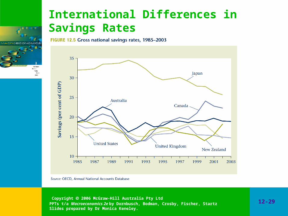
International Differences in Savings Rates
Copyright 2006 McGraw-Hill Australia Pty Ltd PPTs t/a Macroeconomics 2e by Dornbusch, Bodman, Crosby, Fischer, StartzSlides prepared by Dr Monica Keneley.
12-30
International Differences in Savings Rates
• From Figure 12.5:– Significant declines in both private and public sector
savings in the early 1990s contributed to national savings reaching a post-war low of around 15.5% of GDP in late 1992.
– Since then, national savings has increased to 18.9% of GDP.
– This has been entirely due to increased public savings.– Private savings have continued to decline.
Copyright 2006 McGraw-Hill Australia Pty Ltd PPTs t/a Macroeconomics 2e by Dornbusch, Bodman, Crosby, Fischer, StartzSlides prepared by Dr Monica Keneley.
12-31
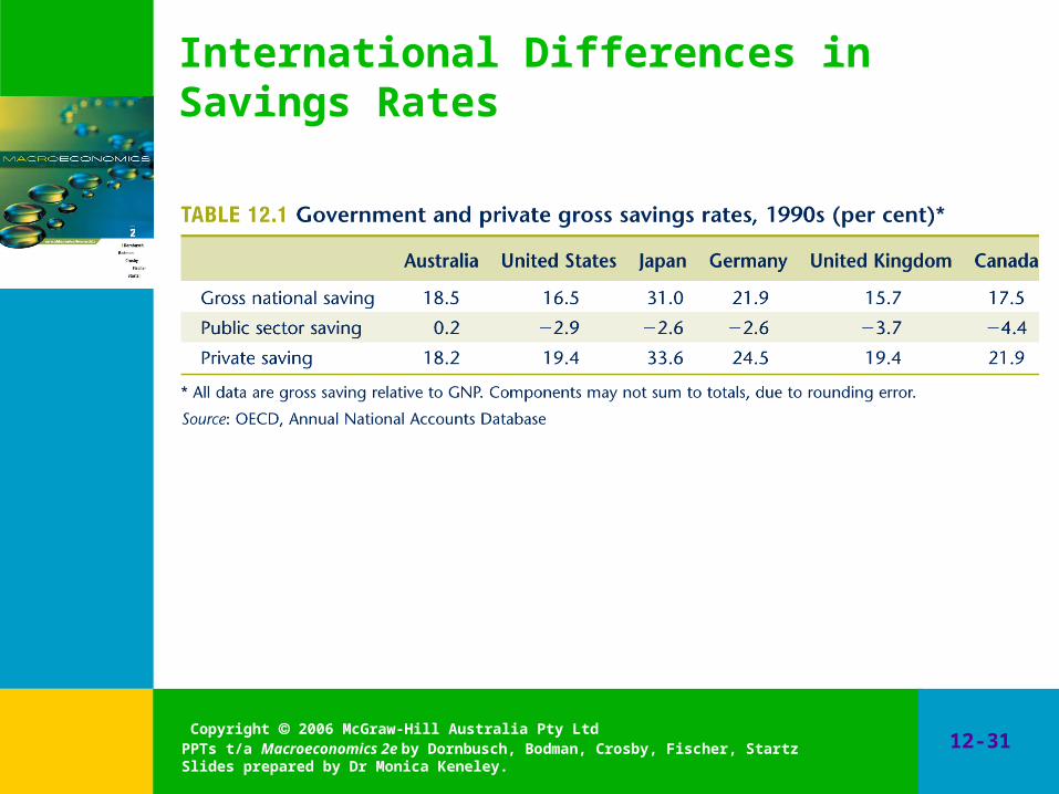
International Differences in Savings Rates

Copyright 2006 McGraw-Hill Australia Pty Ltd PPTs t/a Macroeconomics 2e by Dornbusch, Bodman, Crosby, Fischer, StartzSlides prepared by Dr Monica Keneley.
12-32
International Differences in Savings Rates
• Table 12.1 shows that Australia had an average gross national savings rate in the 1990s of 18.5%.
• This rate is similar to Canada’s (17.5%).
• This rate is higher than the rates for the US (16.5%) and the UK (15.7%).
• However, national saving is considerably lower than Japan’s (31%).

Copyright 2006 McGraw-Hill Australia Pty Ltd PPTs t/a Macroeconomics 2e by Dornbusch, Bodman, Crosby, Fischer, StartzSlides prepared by Dr Monica Keneley.
12-33
International Differences in Savings Rates
• What underlies the trend of savings in Australia and internationally?
– Large budget deficits imply reduced saving in the public sector.
– Changing demographics (such as a larger senior citizen population) account for some of the changes in saving rates over time.
– Australia and other OECD economies find it easier to borrow than most other nations.