Copyright © 2006 Casa Software Ltd. … transmission function is calculated using spectral background informatioin, such that the intensity calibrated spectra can be quantified using

Copyright © 2006 Casa Software Ltd. www.casaxps.com

1. Transmission Correction

Instrumental Considerations and the need for Transmission Correction

Figure 1.1: Logical arrangement of the transfer lens system (electron optics), the hemispherical

analyser (HAS) and the detector system for an XPS instrument.

X-rays illuminate an area of a sample causing electrons to be ejected with a range of energies and directions. The electron optics (conceptually illustrated in Figure 1.1 while a reality is presented in Figure 1.2), which may be a set of electrostatic and/or magnetic lens units, collect a proportion of these emitted electrons defined by those rays that can be transferred through the apertures and focused onto the analyser entrance slit. Electrostatic fields within the hemispherical analyser (HSA) are established to only allow electrons of a given energy (the so called Pass Energy PE) to arrive at the detector slits and onto the detectors themselves. A hemispherical analyser and transfer lenses are typically operated in the two most common modes, namely, Fixed Analyser Transmission (FAT), also known as Constant Analyser Energy (CAE), or Fix Retard Ratio (FRR) also known as Constant Retard Ratio (CRR). In FAT mode, the pass energy of the analyser is held at a constant value and it is entirely the job of the transfer lens system to retard the given kinetic energy channel to the range accepted by the analyser. Most XPS spectra are acquired using FAT. The alternative mode, FRR, scans the lens system but also adjusts the analyser pass energy to

1

Copyright © 2006 Casa Software Ltd. www.casaxps.com maintain a constant value for the quantity “initial electron energy” / “analyser PE”. This mode is typically used for Auger spectra since the energy interval accepted by the detection system (i.e. resolution) increases with kinetic energy and recovers weak peaks at high kinetic energies while restricting the intense low energy background that could do damage to the detection system.

Figure 1.2: A typical research XPS instrument where the hemispherical analyser is clearly visible at

the top of the picture and is connected to the sample chamber by the lens column.

Electrons of a specific initial kinetic energy are measured by setting voltages for the lens system that both focus onto the entrance slit the electrons of the required initial energy and retards their velocity so that their kinetic energy after passing through the transfer lenses matches the pass energy of the hemispherical analyser. To record a spectrum over

2

Copyright © 2006 Casa Software Ltd. www.casaxps.com a range of initial excitation energies it is necessary to scan the voltages applied to these transfer lenses and the prescription for these lens voltages is known as the set of lens functions. These lens functions are typically stored in some configuration file used by the acquisition system. The efficiency with which electrons are sampled by a spectrometer is very dependent on these lens functions and without properly tuned lens functions the performance of an instrument can be severely impaired. Even with a well-tuned system the collection efficiency varies across the many operating modes and it is necessary to characterize an instrument using a corresponding transmission function for each of the lens modes, energy resolutions, aperture settings and spot-sizes of the x-ray source. Transmission correction is central to quantitative XPS. Without proper transmission correction, a comparison of results measured from the same sample using different operating modes for an instrument would show significant variations in atomic concentrations. Thus, following any changes to the lens functions, aperture positions and even changes due to detector aging require the calibration of the intensity scale, which involves computing the transmission functions for any operating mode used in practice.

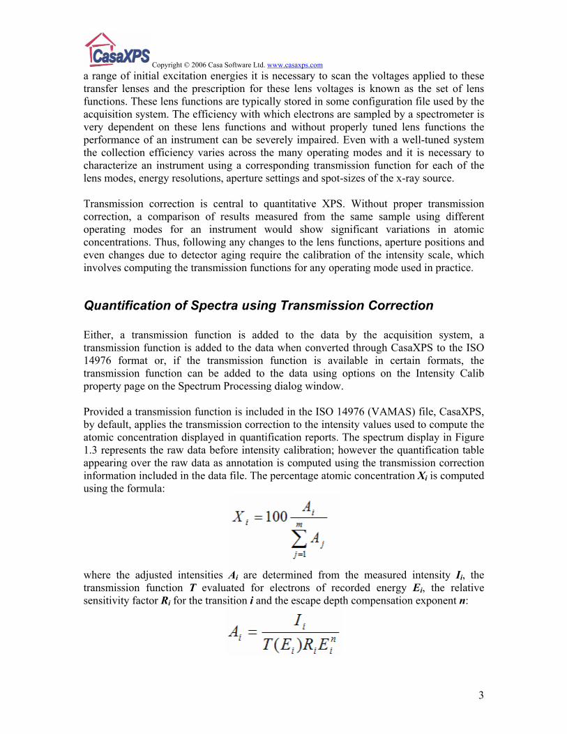
Quantification of Spectra using Transmission Correction Either, a transmission function is added to the data by the acquisition system, a transmission function is added to the data when converted through CasaXPS to the ISO 14976 format or, if the transmission function is available in certain formats, the transmission function can be added to the data using options on the Intensity Calib property page on the Spectrum Processing dialog window. Provided a transmission function is included in the ISO 14976 (VAMAS) file, CasaXPS, by default, applies the transmission correction to the intensity values used to compute the atomic concentration displayed in quantification reports. The spectrum display in Figure 1.3 represents the raw data before intensity calibration; however the quantification table appearing over the raw data as annotation is computed using the transmission correction information included in the data file. The percentage atomic concentration Xi is computed using the formula:

where the adjusted intensities Ai are determined from the measured intensity Ii, the transmission function T evaluated for electrons of recorded energy Ei, the relative sensitivity factor Ri for the transition i and the escape depth compensation exponent n:

3

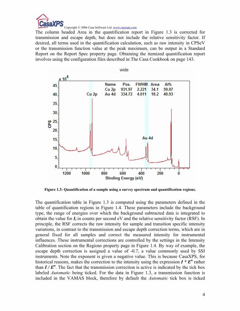
Copyright © 2006 Casa Software Ltd. www.casaxps.com The column headed Area in the quantification report in Figure 1.3 is corrected for transmission and escape depth, but does not include the relative sensitivity factor. If desired, all terms used in the quantification calculation, such as raw intensity in CPSeV or the transmission function value at the peak maximum, can be output in a Standard Report on the Report Spec property page. Obtaining the itemized quantification report involves using the configuration files described in The Casa Cookbook on page 143.

Figure 1.3: Quantification of a sample using a survey spectrum and quantification regions.

The quantification table in Figure 1.3 is computed using the parameters defined in the table of quantification regions in Figure 1.4. These parameters include the background type, the range of energies over which the background subtracted data is integrated to obtain the value for Ii in counts per second eV and the relative sensitivity factor (RSF). In principle, the RSF corrects the raw intensity for sample and transition specific intensity variations, in contrast to the transmission and escape depth correction terms, which are in general fixed for all samples and correct the measured intensity for instrumental influences. These instrumental corrections are controlled by the settings in the Intensity Calibration section on the Regions property page in Figure 1.4. By way of example, the escape depth correction is assigned a value of -0.7, a value commonly used by SSI instruments. Note the exponent is given a negative value. This is because CasaXPS, for historical reasons, makes the correction to the intensity using the expression I * En rather than I / En. The fact that the transmission correction is active is indicated by the tick box labeled Automatic being ticked. For the data in Figure 1.3, a transmission function is included in the VAMAS block, therefore by default the Automatic tick box is ticked

4

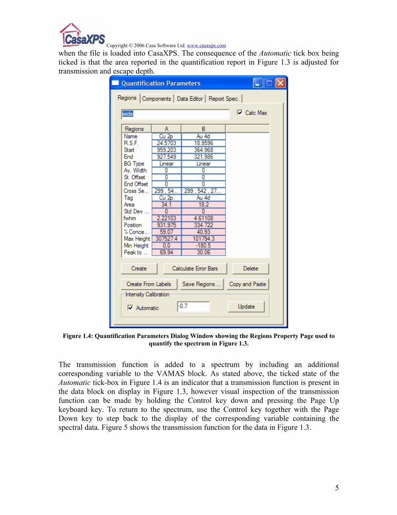
Copyright © 2006 Casa Software Ltd. www.casaxps.com when the file is loaded into CasaXPS. The consequence of the Automatic tick box being ticked is that the area reported in the quantification report in Figure 1.3 is adjusted for transmission and escape depth.

Figure 1.4: Quantification Parameters Dialog Window showing the Regions Property Page used to

quantify the spectrum in Figure 1.3.

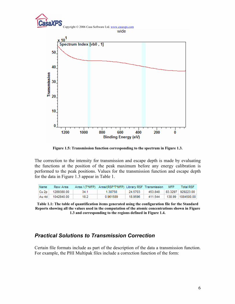
The transmission function is added to a spectrum by including an additional corresponding variable to the VAMAS block. As stated above, the ticked state of the Automatic tick-box in Figure 1.4 is an indicator that a transmission function is present in the data block on display in Figure 1.3, however visual inspection of the transmission function can be made by holding the Control key down and pressing the Page Up keyboard key. To return to the spectrum, use the Control key together with the Page Down key to step back to the display of the corresponding variable containing the spectral data. Figure 5 shows the transmission function for the data in Figure 1.3.

5


6

Figure 1.5: Transmission function corresponding to the spectrum in Figure 1.3.

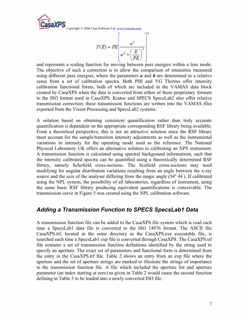
The correction to the intensity for transmission and escape depth is made by evaluating the functions at the position of the peak maximum before any energy calibration is performed to the peak positions. Values for the transmission function and escape depth for the data in Figure 1.3 appear in Table 1.

Table 1.1: The table of quantification items generated using the configuration file for the Standard

Reports showing all the values used in the computation of the atomic concentrations shown in Figure 1.3 and corresponding to the regions defined in Figure 1.4.

Practical Solutions to Transmission Correction Certain file formats include as part of the description of the data a transmission function. For example, the PHI Multipak files include a correction function of the form:


7

and represents a scaling function for moving between pass energies within a lens mode. The objective of such a correction is to allow the comparison of intensities measured using different pass energies, where the parameters a and b are determined in a relative sense from a set of calibration spectra. Both PHI and VG Thermo offer intensity calibration functional forms, both of which are included in the VAMAS data block created by CasaXPS when the data is converted from either of these proprietary formats to the ISO format used in CasaXPS. Kratos and SPECS SpecsLab2 also offer relative transmission correction; these transmission functions are written into the VAMAS files exported from the Vision Processing and SpecsLab2 systems. A solution based on obtaining consistent quantification rather than truly accurate quantification is dependent on the appropriate corresponding RSF library being available. From a theoretical perspective, this is not an attractive solution since the RSF library must account for the sample/transition intensity adjustments as well as the instrumental variations in intensity for the operating mode used as the reference. The National Physical Laboratory UK offers an alternative solution to calibrating an XPS instrument. A transmission function is calculated using spectral background informatioin, such that the intensity calibrated spectra can be quantified using a theoretically determined RSF library, namely Schofield cross-sections. The Scofield cross-sections may need modifying for angular distribution variations resulting from an angle between the x-ray source and the axis of the analyser differing from the magic angle (54o 44’). If calibrated using the NPL system, the possibility of all laboratories, regardless of instrument, using the same basic RSF library producing equivalent quantifications is conceivable. The transmission curve in Figure 5 was created using the NPL calibration software.

Adding a Transmission Function to SPECS SpecsLab1 Data A transmission function file can be added to the CasaXPS file system which is read each time a SpecsLab1 data file is converted to the ISO 14976 format. The ASCII file CasaXPS.trf, located in the same directory as the CasaXPS.exe executable file, is searched each time a SpecsLab1 exp file is converted through CasaXPS. The CasaXPS.trf file contains a set of transmission function definitions identified by the string used to specify an aperture. The exact set of parameters and functional form is determined from the entry in the CasaXPS.trf file. Table 2 shows an entry from an exp file where the aperture and the set of aperture strings are marked to illustrate the strings of importance to the transmission function file. A file which included the aperture list and aperture parameter (an index starting at zero) as given in Table 2 would cause the second function defining in Table 3 to be loaded into a newly converted ISO file.

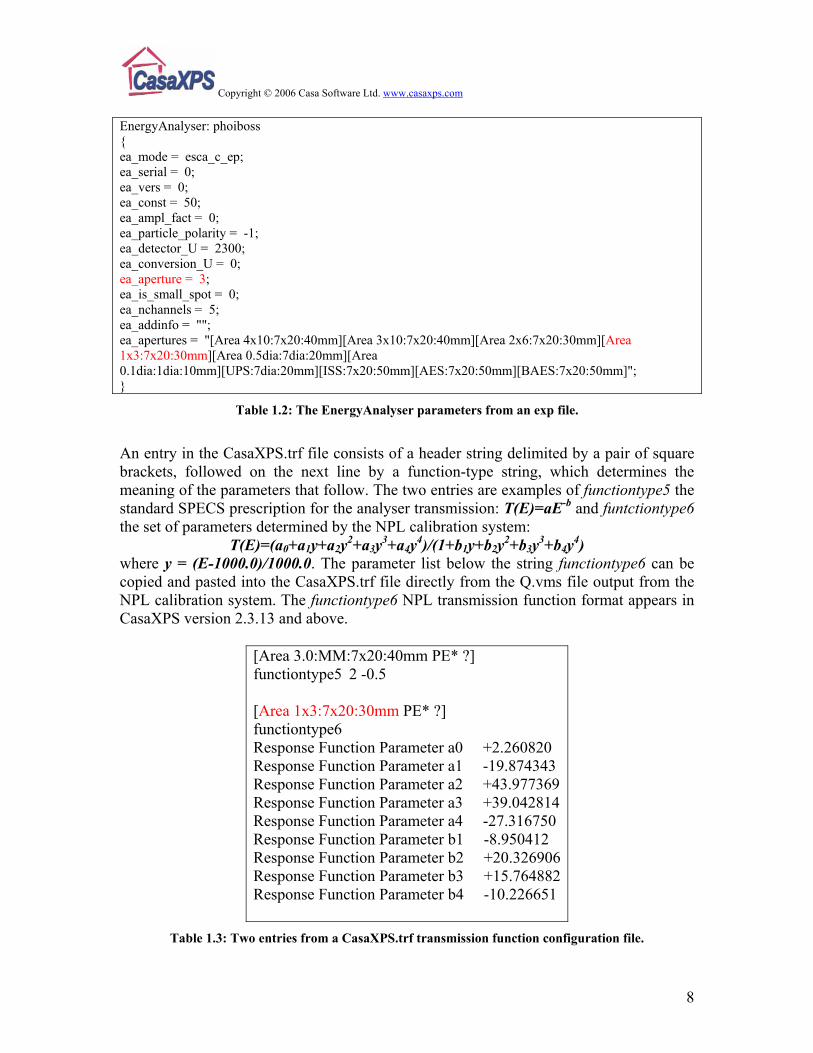
Copyright © 2006 Casa Software Ltd. www.casaxps.com EnergyAnalyser: phoiboss { ea_mode = esca_c_ep; ea_serial = 0; ea_vers = 0; ea_const = 50; ea_ampl_fact = 0; ea_particle_polarity = -1; ea_detector_U = 2300; ea_conversion_U = 0; ea_aperture = 3; ea_is_small_spot = 0; ea_nchannels = 5; ea_addinfo = ""; ea_apertures = "[Area 4x10:7x20:40mm][Area 3x10:7x20:40mm][Area 2x6:7x20:30mm][Area 1x3:7x20:30mm][Area 0.5dia:7dia:20mm][Area 0.1dia:1dia:10mm][UPS:7dia:20mm][ISS:7x20:50mm][AES:7x20:50mm][BAES:7x20:50mm]"; }

Table 1.2: The EnergyAnalyser parameters from an exp file.

An entry in the CasaXPS.trf file consists of a header string delimited by a pair of square brackets, followed on the next line by a function-type string, which determines the meaning of the parameters that follow. The two entries are examples of functiontype5 the standard SPECS prescription for the analyser transmission: T(E)=aE-b and funtctiontype6 the set of parameters determined by the NPL calibration system:

T(E)=(a0+a1y+a2y2+a3y3+a4y4)/(1+b1y+b2y2+b3y3+b4y4) where y = (E-1000.0)/1000.0. The parameter list below the string functiontype6 can be copied and pasted into the CasaXPS.trf file directly from the Q.vms file output from the NPL calibration system. The functiontype6 NPL transmission function format appears in CasaXPS version 2.3.13 and above.

[Area 3.0:MM:7x20:40mm PE* ?] functiontype5 2 -0.5 [Area 1x3:7x20:30mm PE* ?] functiontype6 Response Function Parameter a0 +2.260820 Response Function Parameter a1 -19.874343 Response Function Parameter a2 +43.977369 Response Function Parameter a3 +39.042814 Response Function Parameter a4 -27.316750 Response Function Parameter b1 -8.950412 Response Function Parameter b2 +20.326906 Response Function Parameter b3 +15.764882 Response Function Parameter b4 -10.226651

Table 1.3: Two entries from a CasaXPS.trf transmission function configuration file.

8


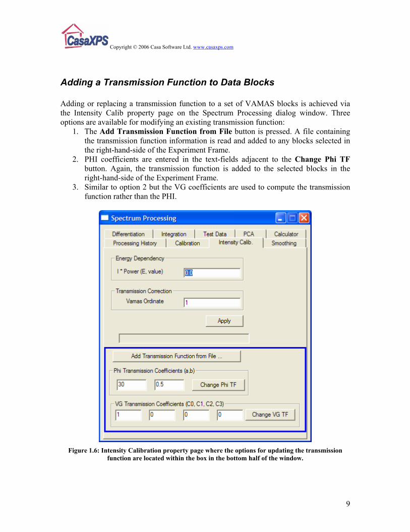
Adding a Transmission Function to Data Blocks Adding or replacing a transmission function to a set of VAMAS blocks is achieved via the Intensity Calib property page on the Spectrum Processing dialog window. Three options are available for modifying an existing transmission function:

1. The Add Transmission Function from File button is pressed. A file containing the transmission function information is read and added to any blocks selected in the right-hand-side of the Experiment Frame.

2. PHI coefficients are entered in the text-fields adjacent to the Change Phi TF button. Again, the transmission function is added to the selected blocks in the right-hand-side of the Experiment Frame.

3. Similar to option 2 but the VG coefficients are used to compute the transmission function rather than the PHI.

Figure 1.6: Intensity Calibration property page where the options for updating the transmission

function are located within the box in the bottom half of the window.

9

Copyright © 2006 Casa Software Ltd. www.casaxps.com Add Transmission Function from File There are three file formats accepted by the Add Transmission Function from File button:

1. A simple ASCII format where the first line is an integer format number, which must be 1. The next line is a positive integer specifying the number of energy, transmission function pairs which follow, one pair per line. The values for the energy and transmission function values must be separated by a space or a TAB.

2. A Q.vms file generated by the NPL Calibration system. The Q.vms file provides a VAMAS description of the transmission function, followed by the parameters and the results of the calibration process. When the Q.vms file is read into CasaXPS, it is the parameter set which is used to compute the transmission function, the VAMAS fields are ignored.

3. A CasaXPS.trf formatted file. When a SpecsLab1 exp is converted, two strings are added to the VAMAS block comment tagged with the prefix “TRF STRING1:” and “TRF STRING2:”. These strings are taken from the aperture list in the exp file and are used to extract a transmission function, on a block by block basis, from the CasaXPS.trf formatted file.

Transmission functions read from file are added to all data blocks selected in the right-hand-side prior to selecting the button.

10


2. Relative Sensitivity Factors and Instrument Geometry In an ideal world, if a sample were analysed using a range of different instruments, the results presented as atomic concentrations would be entirely consistent regardless of type of XPS instrument used to make the measurements. The consistency of these measurements represents the precision with which these measurements can be made by the instrumentation in use. The accuracy obtained for the atomic concentrations is determined by the relative sensitivity factors (RSFs) used to scale the measured intensities for the different elements. Again, in an ideal world, a single set of RSFs offering the relative intensity of photoelectric lines for each nl-electron observed for a given x-ray anode would exist and could be applied to all samples. The goal of absolute accuracy based on a single set of RSFs for all samples is unattainable for many reasons; however the concept of relative accuracy is the accepted goal for many analysts using XPS. That is, assuming all instruments were calibrated for intensity variations due to transmission, then one would like to use a common RSF library to ensure the same quantification is reported irrespective of which instrument made the analysis. Scofield (J. Electron Spectrosc. Relat. Phenom. 8, 129 (1976)) compiled a set of photo-ionisation cross-sections for aluminium and magnesium x-ray sources. In principle these describe the relative intensities for the various photoelectric lines observed in the energy spectra. In practice, the principle of this statement is only true provided the x-ray source and energy analyser are at the, so called, magic angle of 54o 44’. For all other angles between these two mechanical components the relative sensitivity for the different transitions changes due to the angular distribution of photoelectrons ionized by un-polarized light impinging on an nl-shell electron. The equation describing the angular distribution is given by (Reilman et al, J. Electron Spectrosc. Relat. Phenom. 8, 389 (1976)):

. Where ε is the photoelectron energy, σnl(ε) is the cross-section for photo-ionizing an nl electron (Scofield), θ is the angle between the photon and the photoelectron direction (Figure 2.1) and

. βnl(ε), the asymmetry parameter, like σnl(ε) also depends on the wave function. The complexity of the intensity variation with transition is removed for instruments such that P2(cos θ)=0 or θ = 54o 44’, for which the term involving βnl(ε) drops out of the equation above. For instruments where the angle θ differs from the magic angle, the Scofield cross-sections must be corrected to account for the non-zero term involving βnl(ε). Sadly, most instruments to date do not use the magic angle between the analyser and x-ray source and therefore tables of asymmetry parameters are required to modify the RSF tables containing values appropriate for the magic angle configuration.

11


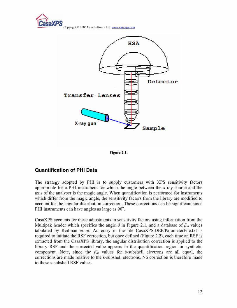
Figure 2.1:

Quantification of PHI Data The strategy adopted by PHI is to supply customers with XPS sensitivity factors appropriate for a PHI instrument for which the angle between the x-ray source and the axis of the analyser is the magic angle. When quantification is performed for instruments which differ from the magic angle, the sensitivity factors from the library are modified to account for the angular distribution correction. These corrections can be significant since PHI instruments can have angles as large as 90o. CasaXPS accounts for these adjustments to sensitivity factors using information from the Multipak header which specifies the angle θ in Figure 2.1, and a database of βnl values tabulated by Reilman et al. An entry in the file CasaXPS.DEF/ParameterFile.txt is required to initiate the RSF correction, but once defined (Figure 2.2), each time an RSF is extracted from the CasaXPS library, the angular distribution correction is applied to the library RSF and the corrected value appears in the quantification region or synthetic component. Note, since the βnl values for s-subshell electrons are all equal, the corrections are made relative to the s-subshell electrons. No correction is therefore made to these s-subshell RSF values.

12


13

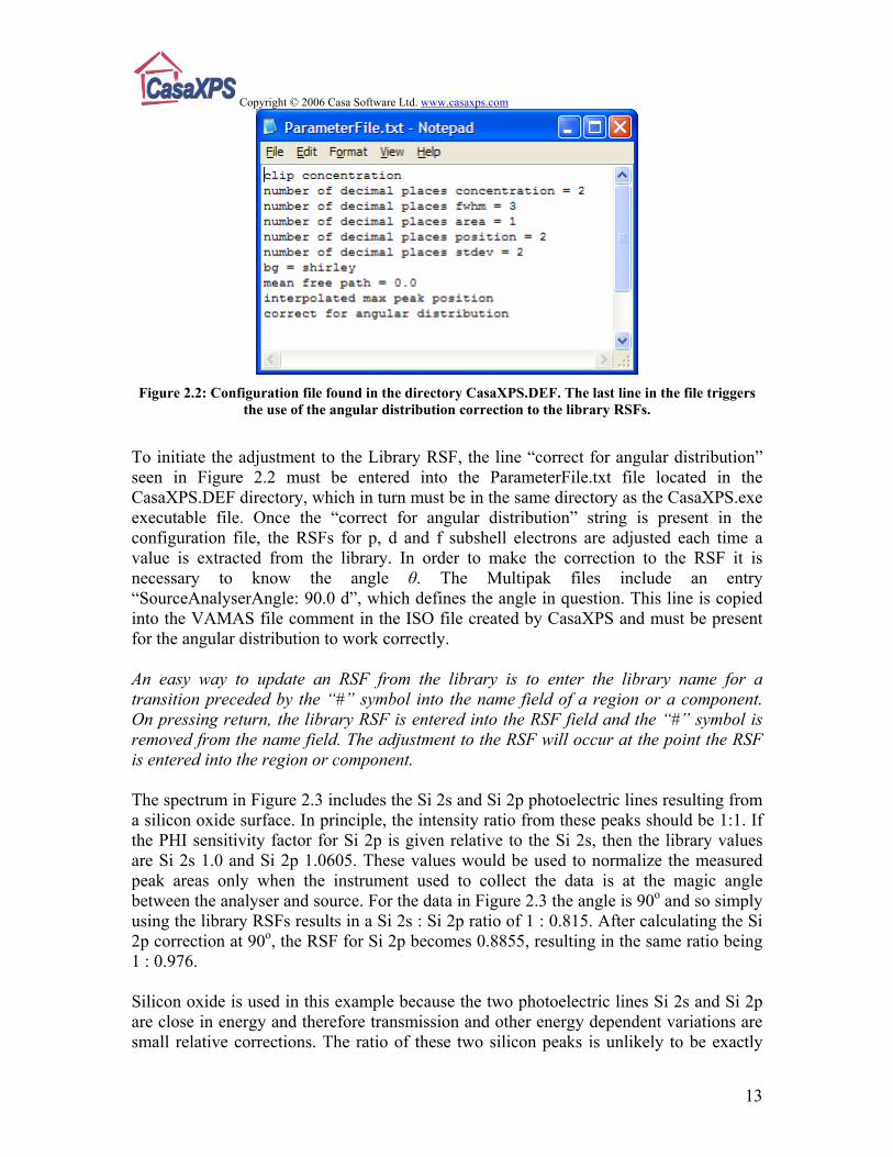
Figure 2.2: Configuration file found in the directory CasaXPS.DEF. The last line in the file triggers

the use of the angular distribution correction to the library RSFs.

To initiate the adjustment to the Library RSF, the line “correct for angular distribution” seen in Figure 2.2 must be entered into the ParameterFile.txt file located in the CasaXPS.DEF directory, which in turn must be in the same directory as the CasaXPS.exe executable file. Once the “correct for angular distribution” string is present in the configuration file, the RSFs for p, d and f subshell electrons are adjusted each time a value is extracted from the library. In order to make the correction to the RSF it is necessary to know the angle θ. The Multipak files include an entry “SourceAnalyserAngle: 90.0 d”, which defines the angle in question. This line is copied into the VAMAS file comment in the ISO file created by CasaXPS and must be present for the angular distribution to work correctly. An easy way to update an RSF from the library is to enter the library name for a transition preceded by the “#” symbol into the name field of a region or a component. On pressing return, the library RSF is entered into the RSF field and the “#” symbol is removed from the name field. The adjustment to the RSF will occur at the point the RSF is entered into the region or component. The spectrum in Figure 2.3 includes the Si 2s and Si 2p photoelectric lines resulting from a silicon oxide surface. In principle, the intensity ratio from these peaks should be 1:1. If the PHI sensitivity factor for Si 2p is given relative to the Si 2s, then the library values are Si 2s 1.0 and Si 2p 1.0605. These values would be used to normalize the measured peak areas only when the instrument used to collect the data is at the magic angle between the analyser and source. For the data in Figure 2.3 the angle is 90o and so simply using the library RSFs results in a Si 2s : Si 2p ratio of 1 : 0.815. After calculating the Si 2p correction at 90o, the RSF for Si 2p becomes 0.8855, resulting in the same ratio being 1 : 0.976. Silicon oxide is used in this example because the two photoelectric lines Si 2s and Si 2p are close in energy and therefore transmission and other energy dependent variations are small relative corrections. The ratio of these two silicon peaks is unlikely to be exactly

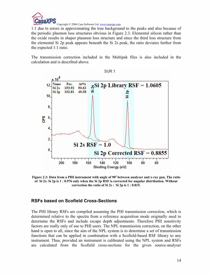
Copyright © 2006 Casa Software Ltd. www.casaxps.com 1:1 due to errors in approximating the true background to the peaks and also because of the periodic plasmon loss structures obvious in Figure 2.3. Elemental silicon rather than the oxide results in shaper plasmon loss structure and since the third loss structure from the elemental Si 2p peak appears beneath the Si 2s peak, the ratio deviates further from the expected 1:1 ratio. The transmission correction included in the Multipak files is also included in the calculation and is described above.

Figure 2.3: Data from a PHI instrument with angle of 90o between analyser and x-ray gun. The ratio

of Si 2s: Si 2p is 1 : 0.976 only when the Si 2p RSF is corrected for angular distribution. Without correction the ratio of Si 2s : Si 2p is 1 : 0.815.

RSFs based on Scofield Cross-Sections The PHI library RSFs are compiled assuming the PHI transmission correction, which is determined relative to the spectra from a reference acquisition mode originally used to determine the RSFs and include escape depth adjustments. Therefore PHI sensitivity factors are really only of use to PHI users. The NPL transmission correction, on the other hand is open to all, since the aim of the NPL system is to determine a set of transmission functions that can be applied in combination with a Scofield-based RSF library to any instrument. Thus, provided an instrument is calibrated using the NPL system and RSFs are calculated from the Scofield cross-sections for the given source-analyser

14

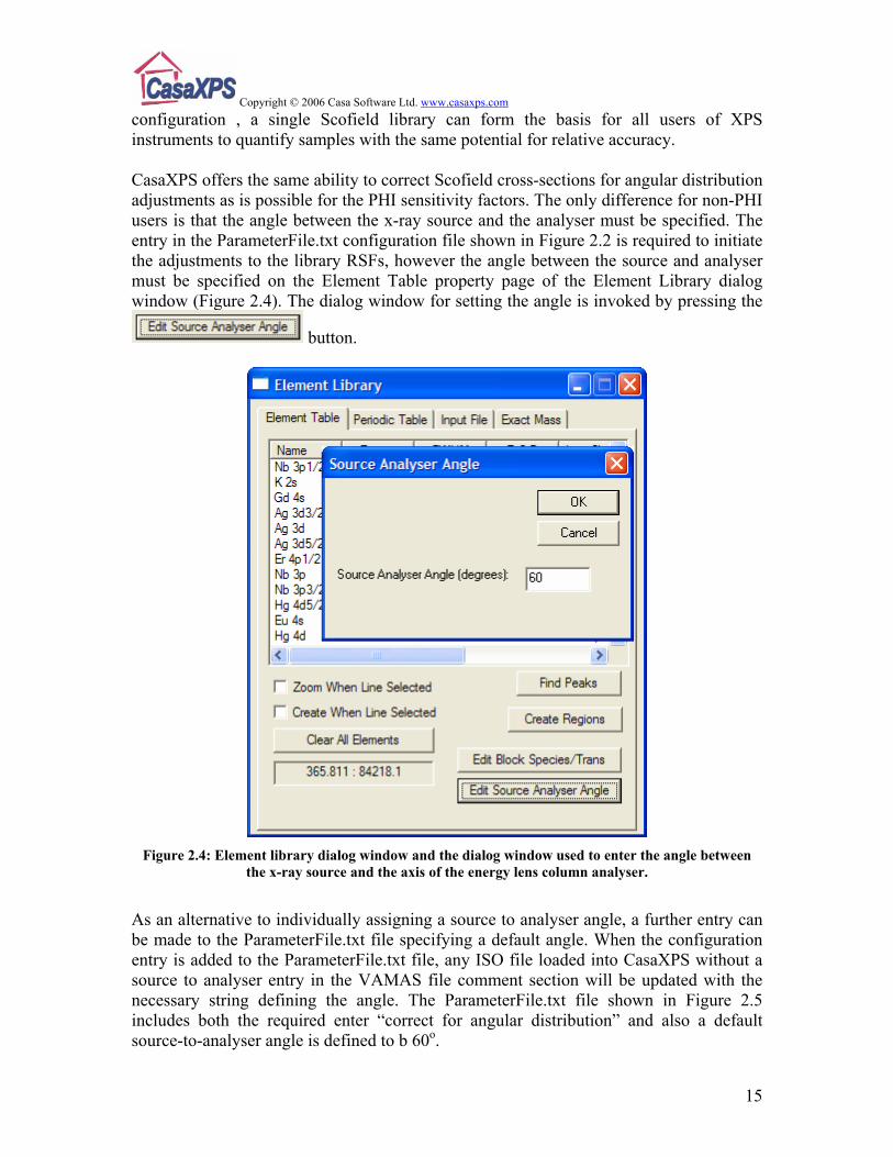
Copyright © 2006 Casa Software Ltd. www.casaxps.com configuration , a single Scofield library can form the basis for all users of XPS instruments to quantify samples with the same potential for relative accuracy. CasaXPS offers the same ability to correct Scofield cross-sections for angular distribution adjustments as is possible for the PHI sensitivity factors. The only difference for non-PHI users is that the angle between the x-ray source and the analyser must be specified. The entry in the ParameterFile.txt configuration file shown in Figure 2.2 is required to initiate the adjustments to the library RSFs, however the angle between the source and analyser must be specified on the Element Table property page of the Element Library dialog window (Figure 2.4). The dialog window for setting the angle is invoked by pressing the

button.

Figure 2.4: Element library dialog window and the dialog window used to enter the angle between

the x-ray source and the axis of the energy lens column analyser.

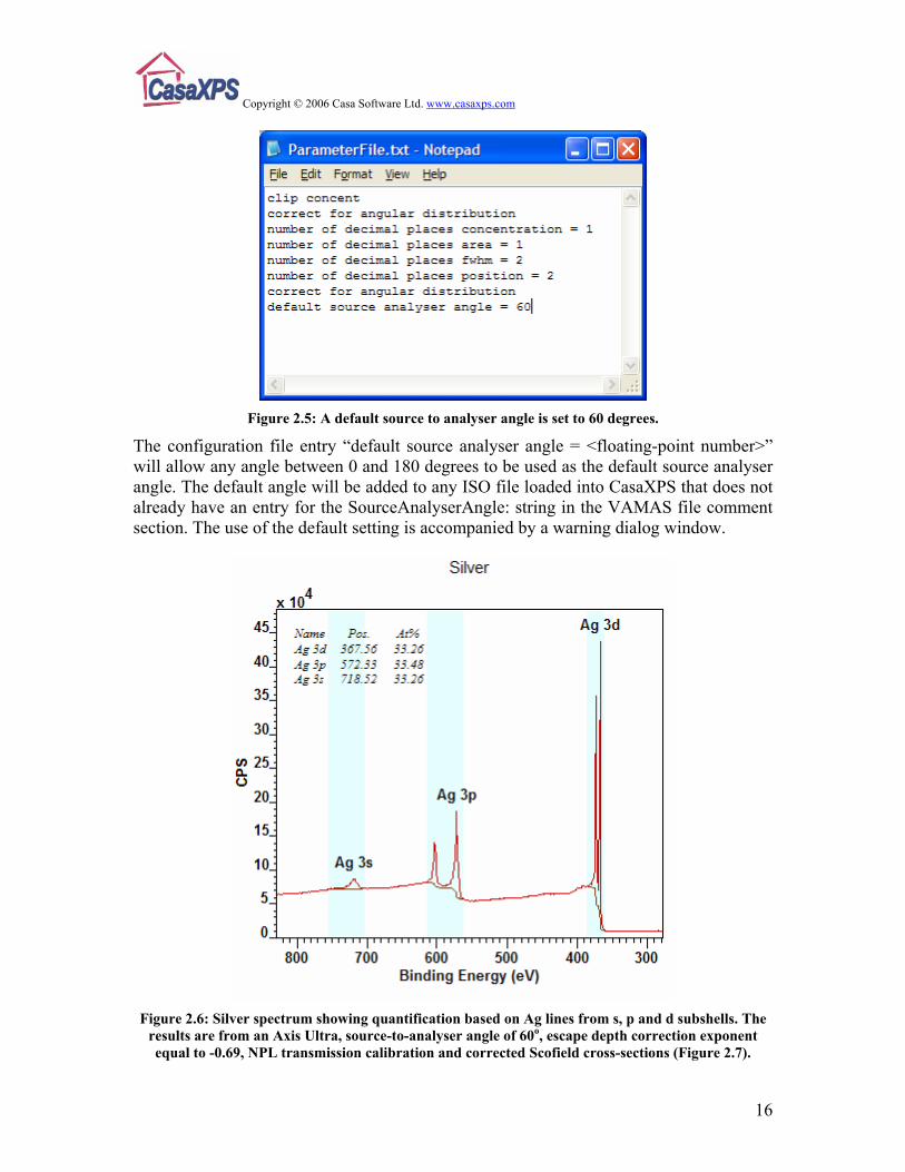
As an alternative to individually assigning a source to analyser angle, a further entry can be made to the ParameterFile.txt file specifying a default angle. When the configuration entry is added to the ParameterFile.txt file, any ISO file loaded into CasaXPS without a source to analyser entry in the VAMAS file comment section will be updated with the necessary string defining the angle. The ParameterFile.txt file shown in Figure 2.5 includes both the required enter “correct for angular distribution” and also a default source-to-analyser angle is defined to b 60o.

15


Figure 2.5: A default source to analyser angle is set to 60 degrees.

The configuration file entry “default source analyser angle = <floating-point number>” will allow any angle between 0 and 180 degrees to be used as the default source analyser angle. The default angle will be added to any ISO file loaded into CasaXPS that does not already have an entry for the SourceAnalyserAngle: string in the VAMAS file comment section. The use of the default setting is accompanied by a warning dialog window.

Figure 2.6: Silver spectrum showing quantification based on Ag lines from s, p and d subshells. The

results are from an Axis Ultra, source-to-analyser angle of 60o, escape depth correction exponent equal to -0.69, NPL transmission calibration and corrected Scofield cross-sections (Figure 2.7).

16


17

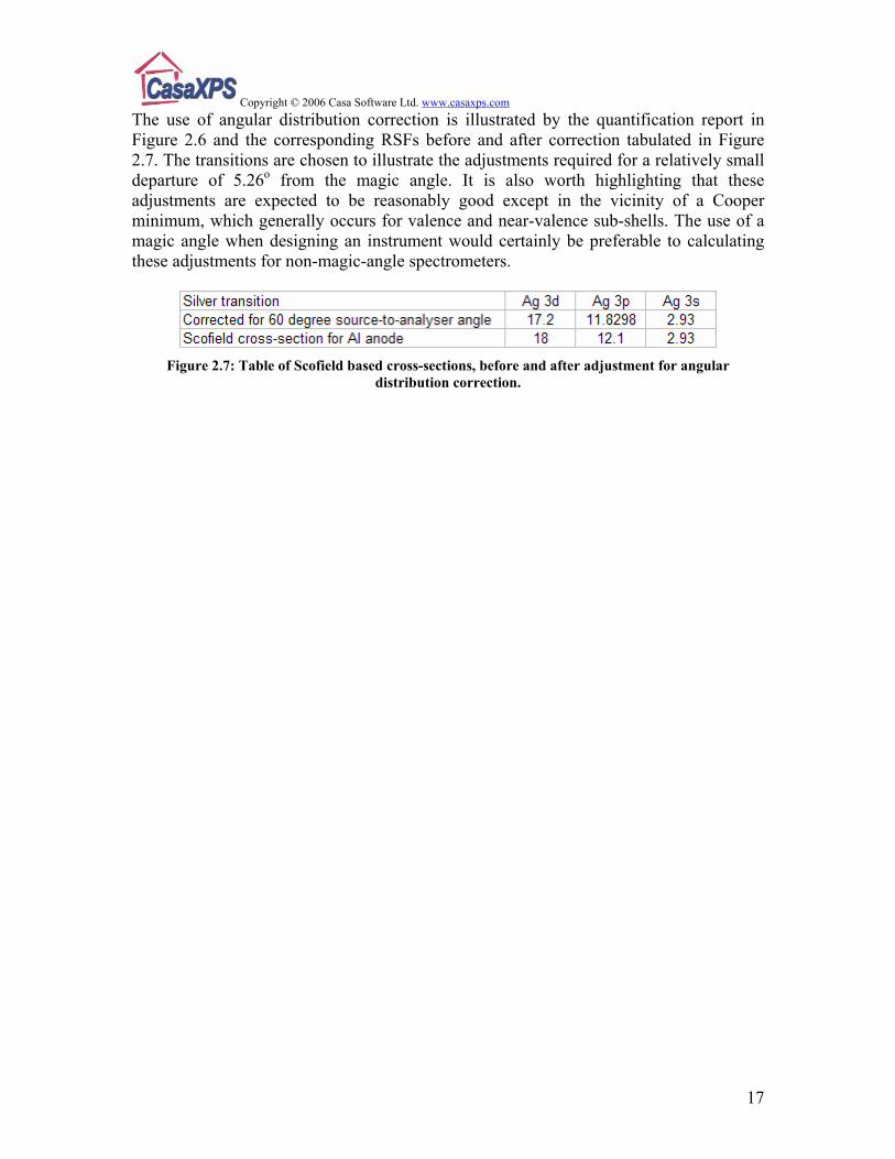
The use of angular distribution correction is illustrated by the quantification report in Figure 2.6 and the corresponding RSFs before and after correction tabulated in Figure 2.7. The transitions are chosen to illustrate the adjustments required for a relatively small departure of 5.26o from the magic angle. It is also worth highlighting that these adjustments are expected to be reasonably good except in the vicinity of a Cooper minimum, which generally occurs for valence and near-valence sub-shells. The use of a magic angle when designing an instrument would certainly be preferable to calculating these adjustments for non-magic-angle spectrometers.

Figure 2.7: Table of Scofield based cross-sections, before and after adjustment for angular

distribution correction.

Documents

Copyright © 2006 Casa Software Ltd. … transmission function is calculated using spectral background informatioin, such that the intensity calibrated spectra can be quantified using