Embed Size (px)
Citation preview

Copyright 2004
Ahmadreza Hedayat
All Rights Reserved

To My Parents
ANALYSIS OF SOURCE-CHANNEL CODING AND EQUALIZATION FOR
WIRELESS COMMUNICATIONS
by
AHMADREZA HEDAYAT, B.S.E.E., M.S.E.E.
DISSERTATION
Presented to the Faculty of
The University of Texas at Dallas
in Partial Fulfillment
of the Requirements
for the Degree of
DOCTOR OF PHILOSOPHY IN ELECTRICAL ENGINEERING
THE UNIVERSITY OF TEXAS AT DALLAS
December 2004

UMI Number: 3151744
31517442005
UMI MicroformCopyright
All rights reserved. This microform edition is protected against unauthorized copying under Title 17, United States Code.
ProQuest Information and Learning Company 300 North Zeeb Road
P.O. Box 1346 Ann Arbor, MI 48106-1346
by ProQuest Information and Learning Company.

ACKNOWLEDGEMENTS
My gratitude and respect first go to my advisor Professor Aria Nosratinia. Aria
supported me technically and financially during my Ph.D. studies. His constant input
has gone towards improving my technical writing style. He has helped his students
in many ways and provided them a friendly environment to carry out research and
collaborate. I would also like to thank Professor Naofal Al-Dhahir, Professor John
Fonseka, and Professor Mohammed Saquib for serving in my supervisory committee
and for their feedback on my dissertation.
During my studies in Dallas I enjoyed friendship and collaboration of many
incredible individuals. I would like to thank them all for the enjoyable and memo-
rable moments we shared. Particularly, I am very grateful to my current and former
colleagues Harsh, Hong Bo, Mohammad, Name, Nikhil, Ramakrishna, Shahab, Todd,
Vijay, and Vimal as well as to wonderful friends Afsaneh, Amir, Dorita, Ehsan, Is-
abella, Mahmoud, Mahnaz, Maryam, Nikki, Rahim, Shahram, and Shayan.
Last, but far from least, my heartfelt thanks go to my family for their support,
encouragement, and care. Most importantly, I would like to thank my parents, to
whom this dissertation is dedicated, for their never-ending love and affection, for the
unconditional support they have given me throughout my life, and for the constant
encouragement during my studies.
v
ANALYSIS OF SOURCE-CHANNEL CODING AND EQUALIZATION FOR
WIRELESS COMMUNICATIONS
Ahmadreza Hedayat, Ph.D.
The University of Texas at Dallas, 2004
Supervisor: Dr. Aria Nosratinia
Future communication applications will include image and video transmission in ad-
dition to mostly-voice services of today. The high rate of these applications, their high
quality of service, and combating the hostile wireless channel require advanced algo-
rithms and techniques in various layers and blocks of the system. This dissertation
looks at the problem of digital data transmission from two perspectives.
In the first part of the dissertation we investigate is the interaction between channel
coding in physical layer and source coding in higher layers. Efficient compression
of finite-alphabet sources requires variable-length codes, however, in the presence of
noisy channels, error propagation in the decoding of these codes severely degrades
performance. To address this problem, we consider redundant entropy codes and
iterative source channel decoding and obtain performance bounds and design crite-
ria for the composite system. We also improve upon the performance of residual
redundancy source channel decoding via an iterative list decoder.
In the second part of the dissertation, we investigate the performance of channel
equalizers in wireless fading channels. Due to the existence of temporal and spatial
interference in wireless channels equalizers must be employed. We analyze various
equalizers in single- and multi-antenna frequency-selective channels.
vi
TABLE OF CONTENTS
Acknowledgements v
Abstract vi
List of Figures x
List of Tables xiii
Chapter 1. Introduction 1
1.1 Outline of the Dissertation . . . . . . . . . . . . . . . . . . . . . . . . 2
Chapter 2. Concatenated Error-correcting Entropy Codes and Channels Codes 4
2.1 Introduction . . . . . . . . . . . . . . . . . . . . . . . . . . . . . . . . 5
2.2 Variable-length Codes with Error-Correcting Capability . . . . . . . . 8
2.3 Trellis Representation of Variable Length Codes . . . . . . . . . . . . 10
2.4 Serial Concatenation of VLC and Channel Codes . . . . . . . . . . . . 11
2.5 Iterative VLC and Channel Decoding . . . . . . . . . . . . . . . . . . 17
2.5.1 SISO Channel Decoder . . . . . . . . . . . . . . . . . . . . . . 17
2.5.2 Bit-Level SISO VLC Decoder . . . . . . . . . . . . . . . . . . . 18
2.5.3 Iterative Decoding and Density Evolution . . . . . . . . . . . . 20
2.6 List-Decoding Serially Concatenated VLC and Channel Codes . . . . 22
2.6.1 List-Decoding of Variable-Length Codes . . . . . . . . . . . . . 23
2.6.2 Proposed Iterative List-Decoder . . . . . . . . . . . . . . . . . 24
2.6.3 Non-Binary CRC . . . . . . . . . . . . . . . . . . . . . . . . . . 25
2.7 Experimental Results . . . . . . . . . . . . . . . . . . . . . . . . . . . 26
2.7.1 Iterative List Decoding . . . . . . . . . . . . . . . . . . . . . . 34
2.8 Chapter Summary . . . . . . . . . . . . . . . . . . . . . . . . . . . . . 35
vii
Chapter 3. Performance of Equalizers in Frequency-Selective Single-AntennaFading Channels 38
3.1 Introduction . . . . . . . . . . . . . . . . . . . . . . . . . . . . . . . . 38
3.2 MLSE Equalizer . . . . . . . . . . . . . . . . . . . . . . . . . . . . . . 39
3.3 Linear Equalizers . . . . . . . . . . . . . . . . . . . . . . . . . . . . . 43
3.3.1 Outage Probability of Linear Equalizers . . . . . . . . . . . . . 49
3.3.2 Simulation Results . . . . . . . . . . . . . . . . . . . . . . . . . 59
3.4 Decision-Feedback Equalizers . . . . . . . . . . . . . . . . . . . . . . . 60
3.5 Chapter Summary . . . . . . . . . . . . . . . . . . . . . . . . . . . . . 61
Chapter 4. Performance of Equalizers in Flat Fading Multiple-Antenna Channels 62
4.1 Introduction . . . . . . . . . . . . . . . . . . . . . . . . . . . . . . . . 62
4.2 Maximum Likelihood Equalizer . . . . . . . . . . . . . . . . . . . . . 64
4.3 Linear Equalizers . . . . . . . . . . . . . . . . . . . . . . . . . . . . . 66
4.3.1 Outage Probability in Separate Spatial Encoding . . . . . . . . 69
4.3.2 Outage Probability in Joint Spatial Encoding . . . . . . . . . . 72
4.3.3 Simulation Results . . . . . . . . . . . . . . . . . . . . . . . . . 78
4.4 Decision-Feedback Equalizers . . . . . . . . . . . . . . . . . . . . . . . 82
4.4.1 Outage Probability in Separate Spatial Encoding . . . . . . . . 83
4.4.2 Outage Probability in Joint Spatial Encoding . . . . . . . . . . 85
4.5 Simulation Results . . . . . . . . . . . . . . . . . . . . . . . . . . . . 85
4.6 Chapter Summary . . . . . . . . . . . . . . . . . . . . . . . . . . . . . 86
Chapter 5. Performance of Equalizers in Frequency-Selective Multiple-AntennaFading Channels 88
5.1 Introduction . . . . . . . . . . . . . . . . . . . . . . . . . . . . . . . . 88
5.2 Maximum Likelihood Equalizer . . . . . . . . . . . . . . . . . . . . . 89
5.3 Linear Equalizers . . . . . . . . . . . . . . . . . . . . . . . . . . . . . 91
5.3.1 ZF-LE . . . . . . . . . . . . . . . . . . . . . . . . . . . . . . . . 92
5.3.2 MMSE-LE . . . . . . . . . . . . . . . . . . . . . . . . . . . . . 95
5.3.3 Simulation Results . . . . . . . . . . . . . . . . . . . . . . . . . 97
5.4 Chapter Summary . . . . . . . . . . . . . . . . . . . . . . . . . . . . . 99
viii
Chapter 6. Conclusions and future work 100
6.1 Contributions . . . . . . . . . . . . . . . . . . . . . . . . . . . . . . . 100
6.2 Future Work . . . . . . . . . . . . . . . . . . . . . . . . . . . . . . . . 102
Bibliography 105
VITA
ix
LIST OF FIGURES
2.1 System block diagram . . . . . . . . . . . . . . . . . . . . . . . . . . 6
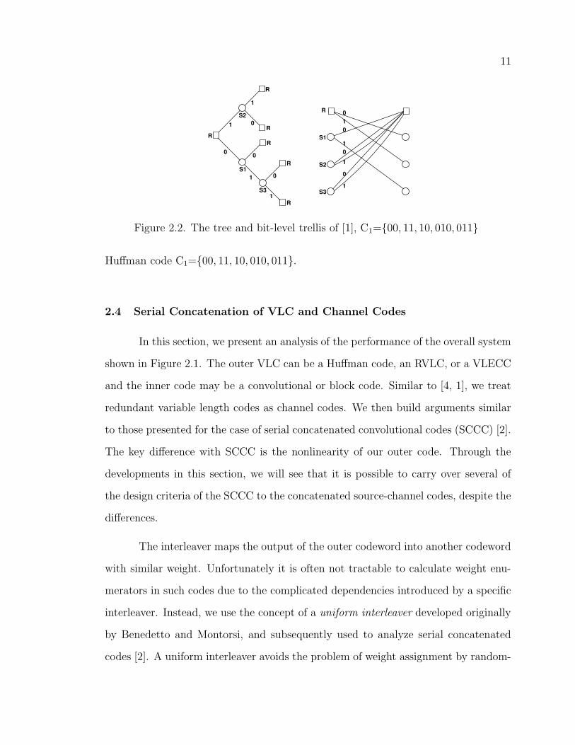
2.2 The tree and bit-level trellis of [1], C1=00, 11, 10, 010, 011 . . . . . 11
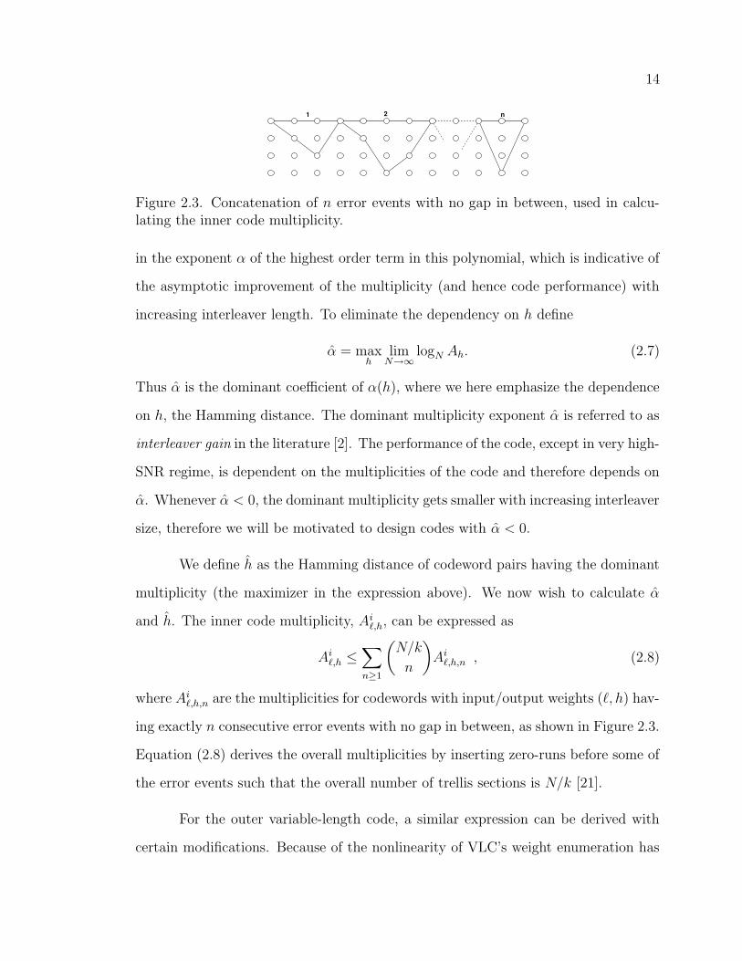
2.3 Concatenation of n error events with no gap in between, used in cal-culating the inner code multiplicity. . . . . . . . . . . . . . . . . . . . 14
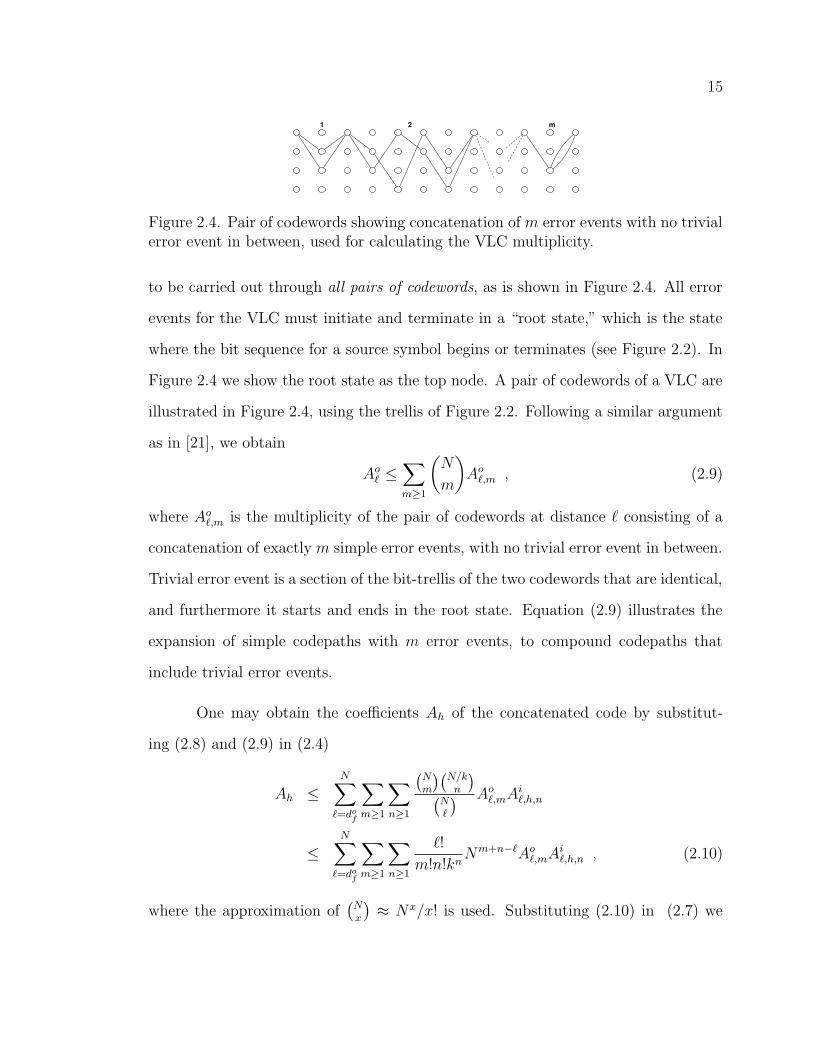
2.4 Pair of codewords showing concatenation of m error events with notrivial error event in between, used for calculating the VLC multiplicity. 15
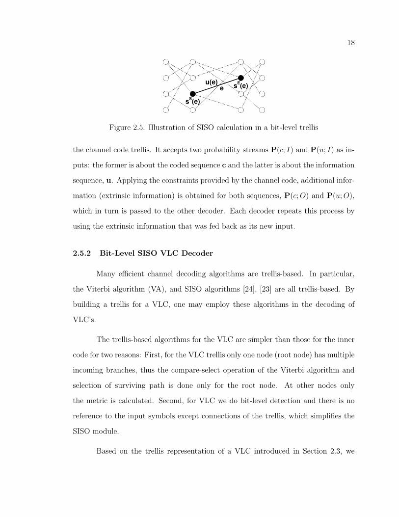
2.5 Illustration of SISO calculation in a bit-level trellis . . . . . . . . . . 18
2.6 Iterative VLC and convolutional decoding . . . . . . . . . . . . . . . 20
2.7 Empirically measured histograms of the output of a channel code andan RVLC SISO modules. From left to right 1,5,10,20 iterations. Eb/N0 =1.5dB . . . . . . . . . . . . . . . . . . . . . . . . . . . . . . . . . . . 21
2.8 Asymptotic analysis of list Viterbi algorithm. . . . . . . . . . . . . . 24
2.9 Iterative- and list-decoding of VLC and channel code . . . . . . . . . 25
2.10 Symbol error rate of C2+CC1, K = 20 and 200 symbols. . . . . . . . 28
2.11 Performance of C2+CC1, C4+CC1(punctured to rate 8/9), and C3+CC3.K = 2000 symbols. . . . . . . . . . . . . . . . . . . . . . . . . . . . . 29
2.12 Approximate Gaussian density evolution of C2+CC1 and C4+CC1(puncturedto rate 8/9), K = 2000 symbols. An instance of the convergence of thedecoders at Eb/N0 = 1.5dB (dashed line staircase) is shown. . . . . . 30
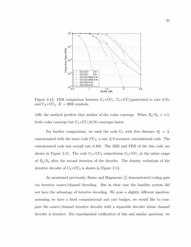
2.13 FER comparison between C2+CC1, C4+CC1(punctured to rate 8/9),and C3+CC3. K = 2000 symbols. . . . . . . . . . . . . . . . . . . . . 31
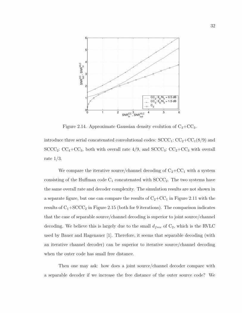
2.14 Approximate Gaussian density evolution of C3+CC3. . . . . . . . . . 32
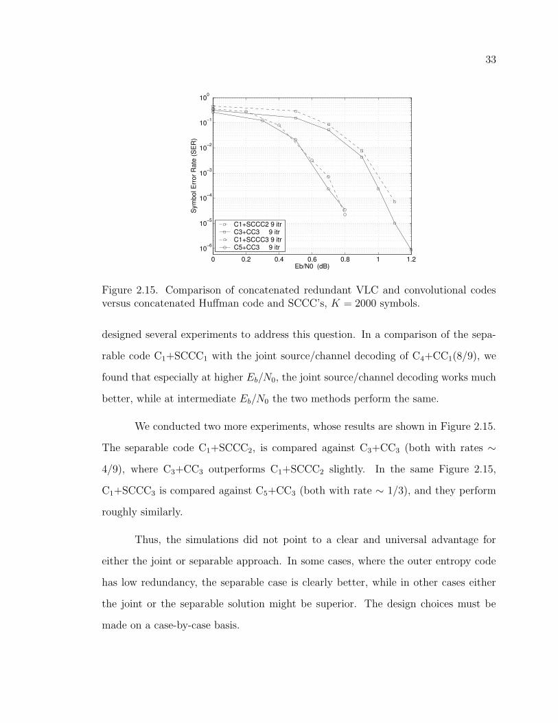
2.15 Comparison of concatenated redundant VLC and convolutional codesversus concatenated Huffman code and SCCC’s, K = 2000 symbols. . 33
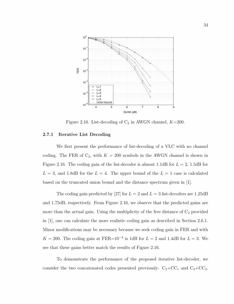
2.16 List-decoding of C2 in AWGN channel, K=200. . . . . . . . . . . . . 34
2.17 Iterative list-decoding of C2+CC1 (dashed) and C3+CC3 (solid line)in AWGN channel, K=500. . . . . . . . . . . . . . . . . . . . . . . . 36
2.18 Iterative list-decoding of C2+CC1 (dashed) and C3+CC3 (solid line)in fully-interleaved Rayleigh channel, K=200. . . . . . . . . . . . . . 36
3.1 Single-carrier frequency-domain equalizer . . . . . . . . . . . . . . . . 44
3.2 Moment generating function of Γ (a) L = ν + 1 = 2, 4, 8 (b) ν = 1 andL = 2, 10, 20, 40. . . . . . . . . . . . . . . . . . . . . . . . . . . . . . . 48
x
3.3 Outage regions of linear equalizers in a two-tap channel, ρ = 10 dB . 52
3.4 Outage probability of ML and linear equalizers, ν = 1, L = 10. ML(solid line), MMSE-LE (solid line marked with ) and ZF-LE (dashedline). The curves correspond, from top left clockwise, to rates R=1,2,4,3bits. . . . . . . . . . . . . . . . . . . . . . . . . . . . . . . . . . . . . 54
3.5 CDF of capacity of the frequency-selective channel (solid line), MMSE-LE (dashed line), and ZF-LE (dashed-dot line) in a two-tap channel,ν = 1, and L = 8. In each plot, the SNR for the left set of curves is 13dB, and 23 dB for the other set. . . . . . . . . . . . . . . . . . . . . . 54
3.6 Outage probability of ML and linear equalizers in a two-tap channelwith 0.5 correlation between the fading coefficients, ν = 1, L = 10.ML (solid line), MMSE-LE (solid line marked with ) and ZF-LE(dashed line). The curves correspond, from top left clockwise, to ratesR=1,2,4,3 bits. . . . . . . . . . . . . . . . . . . . . . . . . . . . . . . 55
3.7 Outage probability of ML and linear equalizers, ν = 2, L = 10. ML(solid line), MMSE-LE (solid line with ) and ZF-LE (dashed line).The curves correspond, from top left clockwise, to rates R=1,2,5,3bits/sec/Hz. . . . . . . . . . . . . . . . . . . . . . . . . . . . . . . . . 58
3.8 Numerical evaluation of CDF of Γ in (3.29) . . . . . . . . . . . . . . . 59
3.9 Symbol error rate of BPSK signaling and linear equalizers (left) ZF-LEν = 1, and L = 4, 10, 20, and (right) ZF-LE versus MMSE-LE ν = 1,and L = 10. . . . . . . . . . . . . . . . . . . . . . . . . . . . . . . . . 60
4.1 Outage probability of linear equalizers. Left: M = N = 2, the pairssolid and dashed lines, from left, correspond to MMSE-LE and ZF-LEfor rates R=1,2,4,10 bits/sec/Hz. Right: M = N = 4, R=4,8,12,16bits/sec/Hz. . . . . . . . . . . . . . . . . . . . . . . . . . . . . . . . . 78
4.2 Outage probability of unconstrained receiver and linear equalizers,Left: M = N = 2, unconstrained receiver (solid line), MMSE-LE(solid line with ) and ZF-LE (dashed line), R=1,2,4,10 bits/sec/Hz.Right: M = N = 4, R=4,8,12,16 bits/sec/Hz. . . . . . . . . . . . . . 79
4.3 Outage probability of MMSE-LE and the upper bound (4.39). M =N = 2, the curves correspond, from left to right, to rates R=1,2,4,10bits/sec/Hz. . . . . . . . . . . . . . . . . . . . . . . . . . . . . . . . . 80
4.4 Outage probability of unconstrained receiver and linear equalizers,M = N = 2 and correlated transmit antennas, ρt = 0.5. Left: uncon-strained receiver (solid line), MMSE-LE (solid line with ) and ZF-LE(dashed line). Right: MMSE outage probability and the upper bound.R=1,2,4,10 bits/sec/Hz. . . . . . . . . . . . . . . . . . . . . . . . . . 81
4.5 CDF of capacity of the unconstrained receiver (solid line), MMSE-LE(dashed line), and ZF-LE (dashed-dot line) in a MIMO channel withM = N = 2. The SNR is, from left to right, 5,10,15,20,25 dB. . . . . 81
4.6 CDF of capacity of the unconstrained receiver (solid line), MMSE-LE(dashed line), and ZF-LE (dashed-dot line) in a MIMO channel with(left) M = 2, N = 4, and (right) M = N = 4. The SNR is, from leftto right, 5,10,15,20,25 dB. . . . . . . . . . . . . . . . . . . . . . . . . 82
xi
4.7 Outage probability of DFE equalizers in separate spatial encoding,M = N = 2. The pairs of solid and dashed lines, from left, correspondto MMSE-DFE and ZF-DFE for rates R = 1, 2, 4, 10 bits/sec/Hz. . . 86
4.8 Outage probability of DFE equalizers in joint spatial encoding, M =N = 2. The pairs of solid and dashed lines, from left, correspond toMMSE-DFE and ZF-DFE for rates R = 1, 2, 4, 10 bits/sec/Hz. Un-constrained equalizer has the same outage probability as MMSE-DFE. 87
5.1 Outage probability of unconstrained and linear equalizers, M = N =2, ν = 1, L = 10. Unconstrained (solid line), MMSE-LE (solid linewith ) and ZF-LE (dashed line). The curves correspond, from topleft clockwise, to rates R=2,4,8,6 bits/sec/Hz. . . . . . . . . . . . . . 98
5.2 Outage probability of MMSE-LE and the upper bound (5.23). M =N = 2, ν = 1, L = 10, the curves correspond, from left to right, torates R=2,4,6,8 bits/sec/Hz. . . . . . . . . . . . . . . . . . . . . . . 99
xii
LIST OF TABLES
2.1 Family variable-length codes used in Section 2.7 . . . . . . . . . . . . 27
2.2 Generator polynomials of convolutional codes used in Section 2.7 (from [2]) 27
xiii
CHAPTER 1
INTRODUCTION
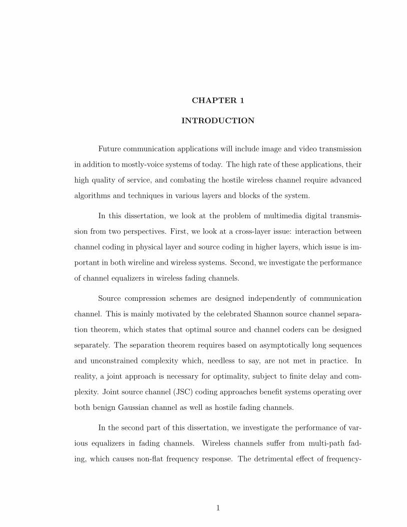
Future communication applications will include image and video transmission
in addition to mostly-voice systems of today. The high rate of these applications, their
high quality of service, and combating the hostile wireless channel require advanced
algorithms and techniques in various layers and blocks of the system.
In this dissertation, we look at the problem of multimedia digital transmis-
sion from two perspectives. First, we look at a cross-layer issue: interaction between
channel coding in physical layer and source coding in higher layers, which issue is im-
portant in both wireline and wireless systems. Second, we investigate the performance
of channel equalizers in wireless fading channels.
Source compression schemes are designed independently of communication
channel. This is mainly motivated by the celebrated Shannon source channel separa-
tion theorem, which states that optimal source and channel coders can be designed
separately. The separation theorem requires based on asymptotically long sequences
and unconstrained complexity which, needless to say, are not met in practice. In
reality, a joint approach is necessary for optimality, subject to finite delay and com-
plexity. Joint source channel (JSC) coding approaches benefit systems operating over
both benign Gaussian channel as well as hostile fading channels.
In the second part of this dissertation, we investigate the performance of var-
ious equalizers in fading channels. Wireless channels suffer from multi-path fad-
ing, which causes non-flat frequency response. The detrimental effect of frequency-
1
2
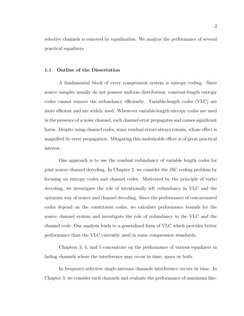
selective channels is removed by equalization. We analyze the performance of several
practical equalizers.
1.1 Outline of the Dissertation
A fundamental block of every compression system is entropy coding. Since
source samples usually do not possess uniform distribution, constant-length entropy
codes cannot remove the redundancy efficiently. Variable-length codes (VLC) are
more efficient and are widely used. Whenever variable-length entropy codes are used
in the presence of a noisy channel, each channel error propagates and causes significant
harm. Despite using channel codes, some residual errors always remain, whose effect is
magnified by error propagation. Mitigating this undesirable effect is of great practical
interest.
One approach is to use the residual redundancy of variable length codes for
joint source channel decoding. In Chapter 2, we consider the JSC coding problem by
focusing on entropy codes and channel codes. Motivated by the principle of turbo
decoding, we investigate the role of intentionally left redundancy in VLC and the
optimum way of source and channel decoding. Since the performance of concatenated
codes depend on the constituent codes, we calculate performance bounds for the
source channel system and investigate the role of redundancy in the VLC and the
channel code. Our analysis leads to a generalized form of VLC which provides better
performance than the VLC currently used in some compression standards.
Chapters 3, 4, and 5 concentrate on the performance of various equalizers in
fading channels where the interference may occur in time, space or both.
In frequency-selective single-antenna channels interference occurs in time. In
Chapter 3, we consider such channels and evaluate the performance of maximum like-
3
lihood, linear, and decision-feedback equalizers and determine their diversity order.
Chapter 4 considers frequency-nonselective multiple-antenna channels where
spatial interference exists. We evaluate the performance of linear and decision-
feedback equalizers for two spatial encoding architectures.
In Chapter 5, we bring the two previous chapters together and consider multiple-
antenna frequency-selective channels where the interference occurs in time and space.
We evaluate the performance of maximum likelihood and linear equalizers and deter-
mine their diversity order.
Finally, Chapter 6 reviews the contribution of the dissertation and discusses
future work.
CHAPTER 2
CONCATENATED ERROR-CORRECTING ENTROPY CODES AND
CHANNELS CODES
Efficient compression of finite-alphabet sources requires variable-length codes
(VLC). However, in the presence of noisy channels, error propagation in the decoding
of VLC severely degrades performance. To address this problem, redundant entropy
codes and iterative source/channel decoding have been suggested, but to date neither
performance bounds nor design criteria for the composite system have been available.
We calculate performance bounds for the source/channel system by generalizing tech-
niques originally developed for serial concatenated convolutional codes (SCCC). Using
this analysis we demonstrate the role of a recursive structure for the inner code and
the distance properties of the outer code. We use density evolution to study the
convergence of our decoders. Finally, we pose the question: under a fixed rate and
complexity constraint, when should we use source-channel decoding (as opposed to
separable decoding). We offer answers in several specific cases.
We also improve the performance of residual redundancy source/channel de-
coding via an iterative list decoder made possible by a non-binary outer CRC code.
We show that the list decoding of VLC’s is beneficial for the redundant codes used in
state-of-art video coding standards. The proposed list-decoder improves the overall
performance significantly in AWGN and fully-interleaved Rayleigh fading channels
even with a short list.
4
5
2.1 Introduction
In this chapter we consider the problem of the transmission of discrete, finite-
alphabet sources over a noisy channel. Since efficient entropy codes are often variable
length codes (VLC), a conventional channel decoding followed by a typical symbol-by-
symbol entropy decoding will result in error propagation, thus a single uncorrected
channel error may result in a long sequence of data errors. This difficulty has led
to a search for error resilient entropy codes. A prominent example is the reversible
variable length code (RVLC) [3] utilized in the video coding standard H.263+ and its
descendants. RVLC consist of a class of codes that have not only a prefix property,
but also a suffix property, thus they can be decoded from both directions.
A more comprehensive attempt at introducing error resilience into variable-
length entropy codes was made by Buttigieg [4, 5], who studied the general class of
entropy codes with error-correction ability, and introduced various sequence decoding
algorithms. Subbalakshmi and Vaisey also provided a trellis for describing VLC’s and
introduced an optimal maximum a posteriori probability decoder for variable-length
encoded sources over a binary-symmetric channel [6, 7].
Error resilient codes mentioned above are not strong enough to handle the er-
ror rates generated by most communication channels, thus a separate layer of channel
coding is usually necessary (see Figure 2.1). In such a concatenated system, itera-
tive decoding methods, originally introduced for channel codes [8, 2], provide another
opportunity for improved source/channel coding. To the best of our knowledge, the
first attempt at iterative decoding of source and channel codes is due to Bauer and
Hagenauer [1, 9], who proposed an iterative (turbo) decoding scheme between a chan-
nel code and the residual redundancy of a reversible variable-length code (RVLC).1
1For an example of iterative source-channel decoding of fixed-length codes see [10].
6
Variable-length code
( size q )
Channel code
u cs
q-ary binary
Non-binary Source
(alphabet size q )Interleaver
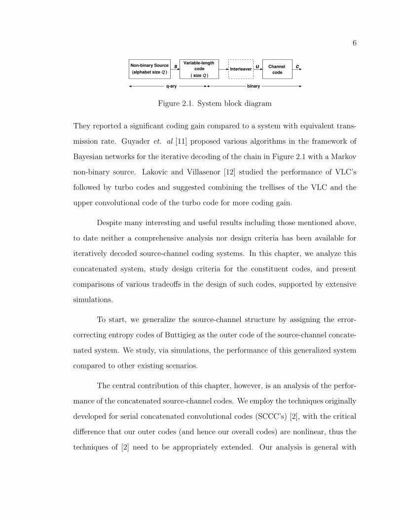
Figure 2.1. System block diagram
They reported a significant coding gain compared to a system with equivalent trans-
mission rate. Guyader et. al [11] proposed various algorithms in the framework of
Bayesian networks for the iterative decoding of the chain in Figure 2.1 with a Markov
non-binary source. Lakovic and Villasenor [12] studied the performance of VLC’s
followed by turbo codes and suggested combining the trellises of the VLC and the
upper convolutional code of the turbo code for more coding gain.
Despite many interesting and useful results including those mentioned above,
to date neither a comprehensive analysis nor design criteria has been available for
iteratively decoded source-channel coding systems. In this chapter, we analyze this
concatenated system, study design criteria for the constituent codes, and present
comparisons of various tradeoffs in the design of such codes, supported by extensive
simulations.
To start, we generalize the source-channel structure by assigning the error-
correcting entropy codes of Buttigieg as the outer code of the source-channel concate-
nated system. We study, via simulations, the performance of this generalized system
compared to other existing scenarios.
The central contribution of this chapter, however, is an analysis of the perfor-
mance of the concatenated source-channel codes. We employ the techniques originally
developed for serial concatenated convolutional codes (SCCC’s) [2], with the critical
difference that our outer codes (and hence our overall codes) are nonlinear, thus the
techniques of [2] need to be appropriately extended. Our analysis is general with
7
respect to the choice of outer VLC’s and inner channel codes: the outer code can be
an RVLC similar to [1, 9, 12] , it can be a VLC with higher redundancy, similar to
the codes introduced in [4], or a VLC with minimum redundancy such as Huffman
codes. The analysis clarifies the roles of the inner and outer codes in the overall per-
formance, allowing us to make statements about the free distance of the outer code
and the desirability of a recursive structure for the inner code. To the best of our
knowledge, these or similar results have not been previously reported in the literature
on source-channel coding.
The analysis and simulations presented in this chapter enable us to make
several observations with practical implications. For example, the method of Bauer
and Hagenauer [9] achieved significant gain compared to systems with similar rate. We
found, however, that it is possible to improve on the scheme of [9], while maintaining
the same overall rate and complexity, by using separable source decoding and an
iteratively decoded SCCC. Thus in this case, investing computational resources into
the channel decoder alone gives better returns in terms of system performance. This
suggests that whenever the entropy code has small free distance (such as the RVLC
used in [9]) one may be better off spending the computational budget mostly on the
inner code and not on iterative decoding between source and channel codes. We also
found that in several cases, even with outer codes having larger free distance, iterative
source channel decoding may yield only a slight advantage compared with a separable
baseline system of equivalent rate and complexity. These findings are expressed in
more detail in the sequel2.
2The contribution of this chapter has been published in [13, 14, 15] and will appear in [16, 17].
8
2.2 Variable-length Codes with Error-Correcting Capability
Buttigieg [4] introduced a class of entropy codes with error-correction ability
under the name of variable-length error-correcting codes (VLECC’s). These codes
have entropy coding property, in the sense that low probability symbols have longer
codewords compared to high-probability symbols. On the other hand, these codes
also have error correction capability, arising from a careful assignment of codewords to
symbols such that a minimum Hamming distance is maintained between all codeword
pairs. Obviously, maintaining a minimum distance introduces redundancy into the
code, such that its average length will be bounded away from the entropy of the
source.
Consider a q-ary source with elements denoted by u, and a variable length
code whose codewords are denoted by b(u). The minimum and maximum length of
b(ui)’s are denoted by `min and `max respectively, and the average length by `ave.
To perform maximum likelihood decoding, we need to consider a sequence of K
codewords. We now define such composite codewords. Assume the source sequence
u = (ui : i = 1, · · · , K) is entropy-encoded to the bit sequence
c = (b(u1), b(u2), · · · , b(uK)) = (c1, c2, · · · , cN) .
Because the codewords b(u) are variable length, the length of the output sequence c,
denoted by N , is variable. This leads to difficulty in analysis, therefore we partition
the overall code C into subcodes Ci such that each partition consists only of codewords
of length i. The free distance of C, denoted df , is defined as the minimum value of
the minimum Hamming distances of the individual binary codes Ci. Note that Ci are
in general nonlinear codes.
Buttigieg [4] calculates the upper bounds for the error event probability of a
VLC in the same manner as convolutional codes, by introducing the average number
9
of converging paths on an appropriate trellis at a given Hamming distance. Unfortu-
nately, this approach is not appropriate for our purposes since, unlike Buttigieg, we
intend to use the variable length codes in concatenation with another code. Instead,
we use the codeword enumeration technique [2]. Considering that N , the length of the
bit-sequence c, is a random variable that takes value in [Nmin, Nmax] = [`minK, `maxK],
the upper bounds for the codeword error probability (frame error rate), PE, and sym-
bol error probability, PS are :
PE ≤Nmax∑
N=Nmin
Pr(N)∑
h≥df
Ah(N)Ph
=∑
h≥df
(
Nmax∑
N=Nmin
Pr(N)Ah(N)
)
Ph (2.1)
PS ≤ 1
K
Nmax∑
N=Nmin
Pr(N)∑
h≥df
Bh(N)Ph
=1
K
∑
h≥df
(
Nmax∑
N=Nmin
Pr(N)Bh(N)
)
Ph , (2.2)
where Ph is the pairwise error probability, which has value Ph = 0.5 erfc(√
hEs/N0)
in AWGN channel, and Ah(N), Bh(N) are multiplicities. Specifically, Ah(N) is the
number of codeword pairs in CN with Hamming distance h. Eventually, we are inter-
ested in the distance between symbol strings corresponding to codeword pairs with
Hamming distance h. The average contribution of two codewords of Hamming dis-
tance h to the Levenshtein distance is denoted Bh(N). Note that Ah(N) and Bh(N)
are normalized by the size of the respective codebooks CN . The exchange of summa-
tions in Equations (2.1) and (2.2) allow us to think of the terms inside parentheses
as equivalent Ah and Bh for the entire code, without the need to consider individual
code partitions separately. It is in fact more convenient to calculate Ah, Bh instead
of Ah(N), Bh(N); see for example [4, 1].
10
Computation of Bh is based on the Levenshtein distance between the two
symbol sequences; dL(ui,uj). The Levenshtein distance is defined as the minimum
number of insertions, deletions or substitutions to transform one symbol sequence
into another [18, 4]. The Levenshtein distance is widely used as an error measure for
VLC’s, justified partly in light of the self-synchronization property of VLC’s [4], and
partly because of the lack of other more meaningful and useful distance measures for
VLC’s.
2.3 Trellis Representation of Variable Length Codes
Various trellis representation for VLC’s have been proposed [6, 9, 1]. Subbalak-
shmi and Vaisey [6] proposed a trellis based on the notion of complete and incomplete
states. The decoder is in a complete state if the most recently received bit completes
a codeword, otherwise it is in an incomplete state. The number of states sums up to
S + `max − 1, where S is the number of codewords. Bauer and Hagenauer proposed a
novel two-dimensional trellis which provides bit-level and symbol-level trellises in its
axis [9]. The maximum number of states depends on the length of the sequence in
bits and symbols and is N − `minK + 1.
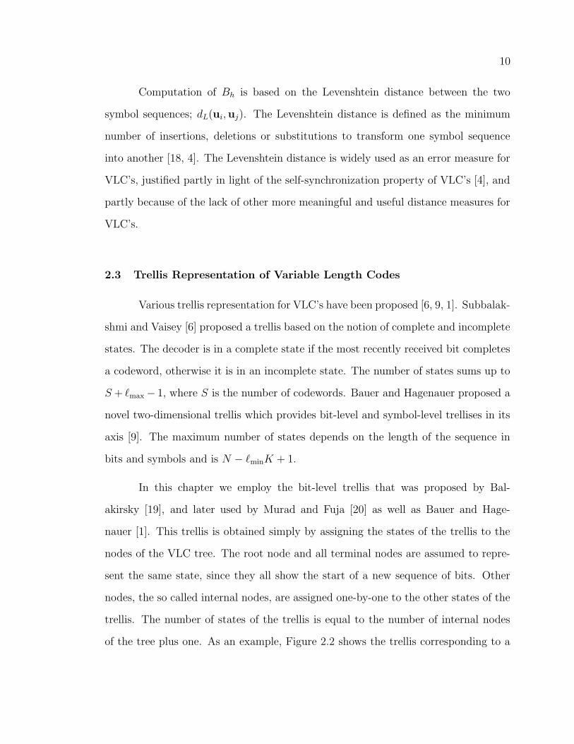
In this chapter we employ the bit-level trellis that was proposed by Bal-
akirsky [19], and later used by Murad and Fuja [20] as well as Bauer and Hage-
nauer [1]. This trellis is obtained simply by assigning the states of the trellis to the
nodes of the VLC tree. The root node and all terminal nodes are assumed to repre-
sent the same state, since they all show the start of a new sequence of bits. Other
nodes, the so called internal nodes, are assigned one-by-one to the other states of the
trellis. The number of states of the trellis is equal to the number of internal nodes
of the tree plus one. As an example, Figure 2.2 shows the trellis corresponding to a
11
0 0
0
01
1
1
1
R
R
R
R
R
R
S1
S2
S3
R
S1
S2
S3
0
0
0
0
1
1
1
1
Figure 2.2. The tree and bit-level trellis of [1], C1=00, 11, 10, 010, 011
Huffman code C1=00, 11, 10, 010, 011.
2.4 Serial Concatenation of VLC and Channel Codes
In this section, we present an analysis of the performance of the overall system
shown in Figure 2.1. The outer VLC can be a Huffman code, an RVLC, or a VLECC
and the inner code may be a convolutional or block code. Similar to [4, 1], we treat
redundant variable length codes as channel codes. We then build arguments similar
to those presented for the case of serial concatenated convolutional codes (SCCC) [2].
The key difference with SCCC is the nonlinearity of our outer code. Through the
developments in this section, we will see that it is possible to carry over several of
the design criteria of the SCCC to the concatenated source-channel codes, despite the
differences.
The interleaver maps the output of the outer codeword into another codeword
with similar weight. Unfortunately it is often not tractable to calculate weight enu-
merators in such codes due to the complicated dependencies introduced by a specific
interleaver. Instead, we use the concept of a uniform interleaver developed originally
by Benedetto and Montorsi, and subsequently used to analyze serial concatenated
codes [2]. A uniform interleaver avoids the problem of weight assignment by random-
12
izing over the space of all possible interleavers: it maps a codeword of weight ` into
all distinct(
N`
)
permutations with equal probability 1/(
N`
)
.
In the following, functions and variables related to the inner code will be
distinguished by the superscript i, and those related to the outer code with superscript
o. Assume the inner code, C i, is a convolutional code with rate Ri = kn. The input-
output weight enumerating function (IOWEF) of the equivalent block code of the
inner convolutional code, with the input length N , is [2]:
Ai(L,H) =N∑
`=0
N/Ri∑
h=dif
Ai`,h(N) L` Hh (2.3)
where Ai`,h(N) represents the number of codewords with weight h generated by infor-
mation words of weight `, and L and H are dummy variables.
We use a uniform interleaver, which maps a codeword of weight ` into all
distinct(
N`
)
permutations with equal probability. The outer VLC has free distance
dof , therefore:
Ah(N) =N∑
`=dof
Ao`(N)Ai
`,h(N)(
N`
) ,
Bh(N) =N∑
`=dof
Bo` (N)Ai
`,h(N)(
N`
) , (2.4)
where Ao`(N) and Bo
` (N) are the associated multiplicities for CN , the length-N sub-
code of the outer code, Ai`,h(N) are the multiplicities of the inner code. Summing
the contributions over all the possible `’s gives the associated coefficients Ah(N) and
Bh(N).
This derivation was facilitated by two facts. First, for two codewords a and
b we have dH(a,b) = dH(π(a), π(b)), where π is the interleaving function. Second,
since the inner code is a linear code, we may speak equivalently of codeword weights
13
or codeword pair distances. In particular, for the inner code, two sequences with
distance ` = dH(π(a), π(b)), will result in two codewords with coded distance h. It
is due to this “invariance” of the interleaver and the linearity of the inner code that
our analysis remains tractable.
We can now calculate the frame error rate, PE, and symbol error rate, PS, of
the concatenated scheme:
PE ≤Nmax∑
N=Nmin
Pr(N)
N/Ri∑
h=df
Ah(N)Ph
=1
2
Nmax∑
N=Nmin
N/Ri∑
h=df
∑
`≥dof
Pr(N)Ao
`(N)Ai`,h(N)
(
N`
) erfc(
√
hEs/N0
)
, (2.5)
PS ≤ 1
K
Nmax∑
N=Nmin
Pr(N)
N/Ri∑
h=df
Bh(N)Ph
=1
2K
Nmax∑
N=Nmin
N/Ri∑
h=df
∑
l≥dof
Pr(N)Bo
l (N)Ail,h(N)
(
N`
) erfc(
√
hEs/N0
)
, (2.6)
where df is the free distance of the concatenated code. Similar to (2.1) and (2.2), the
above results may be presented in terms of equivalent A` and B`. This alternative
form is omitted here for sake of brevity. One may also obtain bounds similar to (2.5)
and (2.6) for the average interleaver size Nave. We note that the above union bounds
can be used with different choices of inner code, for example a convolutional code as
in [1], or a turbo code as in [12].
The asymptotic performance of the bounds above can be studied by looking
at the behavior of coefficients Ah and Bh. We mainly present the analysis for Ah;
similar developments are possible for Bh.
Following [21], the multiplicities Ah can be modeled as a polynomial function
of interleaver size, i.e., Ah ≈ β0Nα + β1N
(α−1) + . . .. We are in particular interested
14
1 2 n
Figure 2.3. Concatenation of n error events with no gap in between, used in calcu-lating the inner code multiplicity.
in the exponent α of the highest order term in this polynomial, which is indicative of
the asymptotic improvement of the multiplicity (and hence code performance) with
increasing interleaver length. To eliminate the dependency on h define
α = maxh
limN→∞
logN Ah. (2.7)
Thus α is the dominant coefficient of α(h), where we here emphasize the dependence
on h, the Hamming distance. The dominant multiplicity exponent α is referred to as
interleaver gain in the literature [2]. The performance of the code, except in very high-
SNR regime, is dependent on the multiplicities of the code and therefore depends on
α. Whenever α < 0, the dominant multiplicity gets smaller with increasing interleaver
size, therefore we will be motivated to design codes with α < 0.
We define h as the Hamming distance of codeword pairs having the dominant
multiplicity (the maximizer in the expression above). We now wish to calculate α
and h. The inner code multiplicity, Ai`,h, can be expressed as
Ai`,h ≤
∑
n≥1
(
N/k
n
)
Ai`,h,n , (2.8)
where Ai`,h,n are the multiplicities for codewords with input/output weights (`, h) hav-
ing exactly n consecutive error events with no gap in between, as shown in Figure 2.3.
Equation (2.8) derives the overall multiplicities by inserting zero-runs before some of
the error events such that the overall number of trellis sections is N/k [21].
For the outer variable-length code, a similar expression can be derived with
certain modifications. Because of the nonlinearity of VLC’s weight enumeration has
15
1 2 m
Figure 2.4. Pair of codewords showing concatenation of m error events with no trivialerror event in between, used for calculating the VLC multiplicity.
to be carried out through all pairs of codewords, as is shown in Figure 2.4. All error
events for the VLC must initiate and terminate in a “root state,” which is the state
where the bit sequence for a source symbol begins or terminates (see Figure 2.2). In
Figure 2.4 we show the root state as the top node. A pair of codewords of a VLC are
illustrated in Figure 2.4, using the trellis of Figure 2.2. Following a similar argument
as in [21], we obtain
Ao` ≤
∑
m≥1
(
N
m
)
Ao`,m , (2.9)
where Ao`,m is the multiplicity of the pair of codewords at distance ` consisting of a
concatenation of exactly m simple error events, with no trivial error event in between.
Trivial error event is a section of the bit-trellis of the two codewords that are identical,
and furthermore it starts and ends in the root state. Equation (2.9) illustrates the
expansion of simple codepaths with m error events, to compound codepaths that
include trivial error events.
One may obtain the coefficients Ah of the concatenated code by substitut-
ing (2.8) and (2.9) in (2.4)
Ah ≤N∑
`=dof
∑
m≥1
∑
n≥1
(
Nm
)(
N/kn
)
(
N`
) Ao`,mAi
`,h,n
≤N∑
`=dof
∑
m≥1
∑
n≥1
`!
m!n!knNm+n−`Ao
`,mAi`,h,n , (2.10)
where the approximation of(
Nx
)
≈ Nx/x! is used. Substituting (2.10) in (2.7) we
16
obtain
α = maxh
(m + n) − ` ≤ b `
dof
c + b `
wmin
c − `, (2.11)
where the bound for the outer code, b `do
fc, reflects the possibility of the concatenation
of error events all with minimum distance dof , while the bound for the inner code,
b `wmin
c, shows the maximum number of concatenated error events with minimum
uncoded weight wmin. For block codes and non-recursive convolutional codes wmin = 1
which results in a positive value for α, thus the concatenated code will not have any
interleaving gain. For recursive convolutional codes wmin = 2 since no finite error
event with w = 1 exists.3 Evaluating the maximum of the right hand side of (2.11)
for the recursive convolutional code results in
α ≤ −bdo
f + 1
2c + 1 (2.12)
offering interleaving gain for frame error rate PE whenever dof is greater than two.4
Depending on whether dof is odd or even h is calculated differently. The design of
recursive convolutional codes is [2, 21].
To summarize, there are two important factors in the performance of source-
channel concatenated codes: the free distance of the outer code and the recursive
structure for the inner code. This was demonstrated by an extension of the techniques
of [2] in order to accommodate the nonlinear codes of interest in source-channel
coding. The design issues of the inner code are similar to the case of ordinary SCCC’s,
which have been well developed in the literature [2, 21].
Our analysis is based on the concept of union bound, which diverges at low
Eb/N0 values (in particular at SNR values below those corresponding to the channel
3In other words, in block codes and non-recursive convolutional codes, a single “1” leads to afinite error event, while in recursive convolutional codes at least two “1”s are needed in the datasequence for a finite error event.
4Similarly, calculations for Bh indicate that the interleaving gain for symbol error rate PS isαB = α − 1.
17
cutoff rate [2]). There is no solid theoretical ground for using union bound analysis
below cutoff rate. However, as has been noted in the literature [2], design criteria
based on these bounds perform surprisingly well even at SNR values where the bounds
do not converge. Our simulations also support that conclusion.
2.5 Iterative VLC and Channel Decoding
Iterative detection (decoding) is possible when a sequence has two or more sets
of concurrent likelihood expressions for a data sequence. These sets of expressions
represent different constraints over the sequence. Obviously, all constraints have to
be satisfied for the detection process. Iterative decoding suggests satisfying each
constraint separately and repeating the process.
In iterative decoding, each decoder in turn processes the available information
about the desired signal, typically log likelihood ratios, thus modifying and hopefully
improving in each iteration the pool of available information on the received signal.
The additional information is called extrinsic information [8, 22]. Extrinsic informa-
tion represents the new information obtained in each half-iteration by applying the
constraint of a constituent decoder. An efficient way to calculate extrinsic information
is via the soft-input soft-output (SISO) algorithm [23]. In the following we discuss
the structure of the SISO module for a channel code as well as a VLC.
2.5.1 SISO Channel Decoder
A soft-output algorithm for channel decoding was introduced in [24]. A
slightly different version of this algorithm, called the SISO module, was introduced
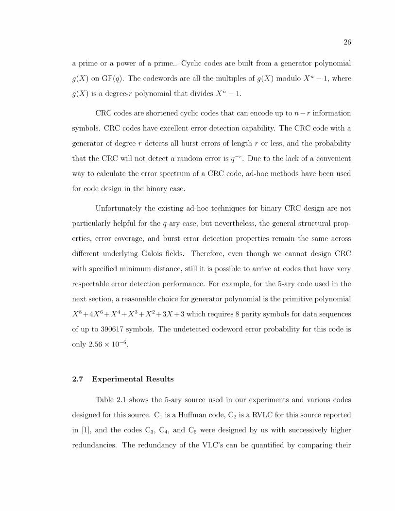
in [23]. We give a system-level description of this block below.
The SISO module for the convolutional code, shown in Figure 2.6, works on
18
sS(e)
sE(e)eu(e)
Figure 2.5. Illustration of SISO calculation in a bit-level trellis
the channel code trellis. It accepts two probability streams P(c; I) and P(u; I) as in-
puts: the former is about the coded sequence c and the latter is about the information
sequence, u. Applying the constraints provided by the channel code, additional infor-
mation (extrinsic information) is obtained for both sequences, P(c; O) and P(u; O),
which in turn is passed to the other decoder. Each decoder repeats this process by
using the extrinsic information that was fed back as its new input.
2.5.2 Bit-Level SISO VLC Decoder
Many efficient channel decoding algorithms are trellis-based. In particular,
the Viterbi algorithm (VA), and SISO algorithms [24], [23] are all trellis-based. By
building a trellis for a VLC, one may employ these algorithms in the decoding of
VLC’s.
The trellis-based algorithms for the VLC are simpler than those for the inner
code for two reasons: First, for the VLC trellis only one node (root node) has multiple
incoming branches, thus the compare-select operation of the Viterbi algorithm and
selection of surviving path is done only for the root node. At other nodes only
the metric is calculated. Second, for VLC we do bit-level detection and there is no
reference to the input symbols except connections of the trellis, which simplifies the
SISO module.
Based on the trellis representation of a VLC introduced in Section 2.3, we
19
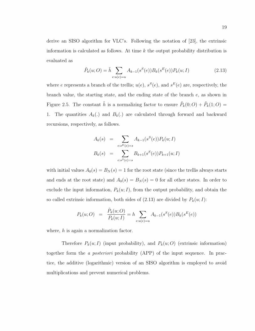
derive an SISO algorithm for VLC’s. Following the notation of [23], the extrinsic
information is calculated as follows. At time k the output probability distribution is
evaluated as
Pk(u; O) = h∑
e:u(e)=u
Ak−1(sS(e))Bk(s
E(e))Pk(u; I) (2.13)
where e represents a branch of the trellis; u(e), sS(e), and sE(e) are, respectively, the
branch value, the starting state, and the ending state of the branch e, as shown in
Figure 2.5. The constant h is a normalizing factor to ensure Pk(0; O) + Pk(1; O) =
1. The quantities Ak(.) and Bk(.) are calculated through forward and backward
recursions, respectively, as follows.
Ak(s) =∑
e:sE(e)=s
Ak−1(sS(e))Pk(u; I)
Bk(s) =∑
e:sS(e)=s
Bk+1(sS(e))Pk+1(u; I)
with initial values A0(s) = BN(s) = 1 for the root state (since the trellis always starts
and ends at the root state) and A0(s) = BN(s) = 0 for all other states. In order to
exclude the input information, Pk(u; I), from the output probability, and obtain the
so called extrinsic information, both sides of (2.13) are divided by Pk(u; I):
Pk(u; O) =Pk(u; O)
Pk(u; I)= h
∑
e:u(e)=u
Ak−1(sS(e))Bk(s
E(e))
where, h is again a normalization factor.
Therefore Pk(u; I) (input probability), and Pk(u; O) (extrinsic information)
together form the a posteriori probability (APP) of the input sequence. In prac-
tice, the additive (logarithmic) version of an SISO algorithm is employed to avoid
multiplications and prevent numerical problems.
20
2.5.3 Iterative Decoding and Density Evolution
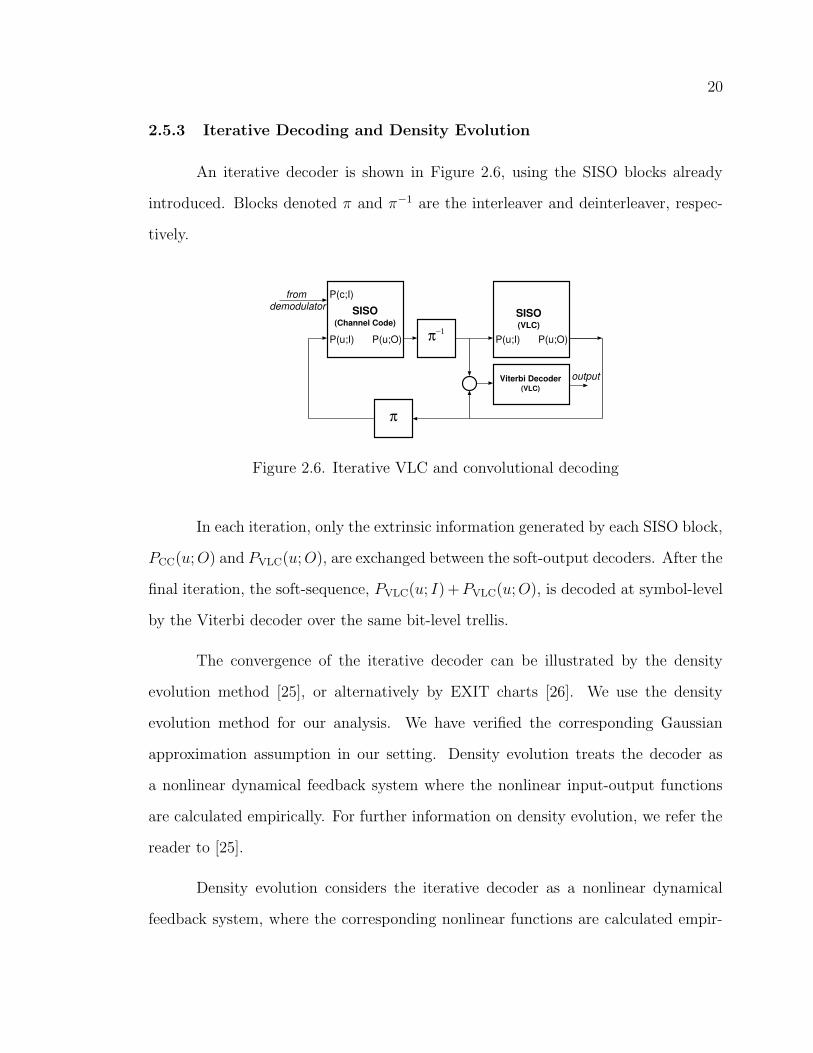
An iterative decoder is shown in Figure 2.6, using the SISO blocks already
introduced. Blocks denoted π and π−1 are the interleaver and deinterleaver, respec-
tively.
SISO(Channel Code)
SISO(VLC)
Viterbi Decoder(VLC)
from demodulator
output
P(u;I) P(u;O)
P(c;I)
P(u;I) P(u;O)
π
π−1
Figure 2.6. Iterative VLC and convolutional decoding
In each iteration, only the extrinsic information generated by each SISO block,
PCC(u; O) and PVLC(u; O), are exchanged between the soft-output decoders. After the
final iteration, the soft-sequence, PVLC(u; I) + PVLC(u; O), is decoded at symbol-level
by the Viterbi decoder over the same bit-level trellis.
The convergence of the iterative decoder can be illustrated by the density
evolution method [25], or alternatively by EXIT charts [26]. We use the density
evolution method for our analysis. We have verified the corresponding Gaussian
approximation assumption in our setting. Density evolution treats the decoder as
a nonlinear dynamical feedback system where the nonlinear input-output functions
are calculated empirically. For further information on density evolution, we refer the
reader to [25].
Density evolution considers the iterative decoder as a nonlinear dynamical
feedback system, where the corresponding nonlinear functions are calculated empir-
21
−10 0 10 20 30 40 50 60 70 800
0.02
0.04
0.06
0.08
0.1
0.12
ΓCC
: Channel code LLR
PD
F(Γ C
C)
PDF of LLRGaussian PDF
−10 0 10 20 30 40 50 60 700
0.05
0.1
0.15
0.2
0.25
0.3
0.35
ΓVLC
: variable−length code LLR
PD
F(Γ V
LC)
PDF of LLRGaussian PDF
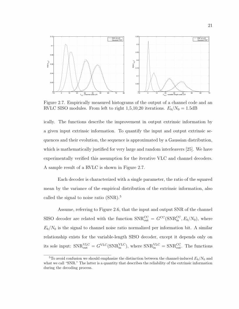
Figure 2.7. Empirically measured histograms of the output of a channel code and anRVLC SISO modules. From left to right 1,5,10,20 iterations. Eb/N0 = 1.5dB
ically. The functions describe the improvement in output extrinsic information by
a given input extrinsic information. To quantify the input and output extrinsic se-
quences and their evolution, the sequence is approximated by a Gaussian distribution,
which is mathematically justified for very large and random interleavers [25]. We have
experimentally verified this assumption for the iterative VLC and channel decoders.
A sample result of a RVLC is shown in Figure 2.7.
Each decoder is characterized with a single parameter, the ratio of the squared
mean by the variance of the empirical distribution of the extrinsic information, also
called the signal to noise ratio (SNR).5
Assume, referring to Figure 2.6, that the input and output SNR of the channel
SISO decoder are related with the function SNRCCout = GCC(SNRCC
in , Eb/N0), where
Eb/N0 is the signal to channel noise ratio normalized per information bit. A similar
relationship exists for the variable-length SISO decoder, except it depends only on
its sole input: SNRVLCout = GVLC(SNRVLC
in ), where SNRVLCin = SNRCC
out. The functions
5To avoid confusion we should emphasize the distinction between the channel-induced Eb/N0 andwhat we call “SNR.” The latter is a quantity that describes the reliability of the extrinsic informationduring the decoding process.
22
GCC and GVLC are evaluated empirically by simulation [25]. One may inspect the
convergence of the iterative decoder by the evolution of the extrinsic information from
one half-iteration to another. This is simply done by plotting SNRCCout versus SNRCC
in ,
GCC curve, and in the same plot, SNRVLCin versus SNRVLC
out , the curve associated with
the inverse of GVLC. When the curves are far apart the decoder converges rapidly. The
convergence may take many iterations if the curves are close, or may not converge
if they intersect. We verify the convergence behavior of some the schemes in the
following section.
2.6 List-Decoding Serially Concatenated VLC and Channel Codes
A list-decoder provides an ordered list of the L most probable sequences in
maximum likelihood sense. Then, an outer error detecting code, usually a cyclic
redundancy check (CRC) code, verifies the validity of the candidates and selects
the error-free sequence, if exists, among the candidates. Two variations of the list
Viterbi-algorithm (LVA) are reported in [27].
The advantage of the list decoder can be explained as follows. In a regular ML
decoder, for an error to occur, the closest codeword to the received sequence must be
an erroneous one. For the list-decoder to make an error, the correct sequence must
lie outside of the L nearest neighbors of the received sequence. This error is less
probable than the corresponding error in the ML decoder.
In a list-decoder, the distance between the received sequence and all the can-
didates determines the performance. Therefore, determining the exact performance
is mathematically intractable. But it is possible to calculate the asymptotic coding
gain, e.g. see [27]. In the case of AWGN channel, a geometrical argument reveals that
the asymptotic coding gain is G = 10 log( 2LL+1
) dB for a list of length L. However,
23
the actual gain is often less due to the multiplicity of the set of L nearest neighbors,
which is neglected in the analysis [27].
2.6.1 List-Decoding of Variable-Length Codes
List-decoders can also be applied for variable-length encoded sequences, given
an appropriate trellis (e.g. the bit-level trellises mentioned earlier). Our list decoding
is constructed with the help of a non-binary CRC code, which verifies the validity of
the L most probable paths in the VLC trellis. The alphabet set of the CRC code
must cover all codewords of the VLC (size q). If q is a power of a prime, it is possible
to construct a q-ary CRC code, otherwise the size of VLC should be extended to the
nearest power of a prime. One can use the a-priori knowledge that these additional
symbols are never present in the data sequence, but only (possibly) present in the
parity sequence.
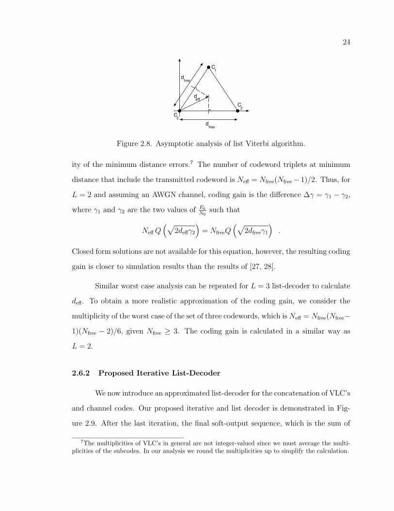
The asymptotic error rate for a list of size L = 2 is based on a simple geometric
construction due to Seshadri and Sundberg [27] (see Figure 2.8). When the three
codewords are pairwise equi-distant, it produces a worst-case error probability. In
this case, the minimum-magnitude noise resulting in an error is shown by the vector
terminating at the center of the triangle. This is an effective minimum distance,
denoted deff, which is larger than dfree/2, explaining the list decoding gain, which is
equal to 10 log( 2LL+1
) dB, as calculated in [27].
This value of asymptotic gain, however, ignores the multiplicities of the mini-
mum distance, and in our case minimum distance error event has high multiplicities6.
Therefore, we augment the asymptotic analysis of [27, 28] for L = 2, 3 list-decoder of
VLC’s so that multiplicities are taken into account. We denote by Nfree the multiplic-
6More information on the distance spectrum of VLC’s is available in [4], and two examples aregiven in [1].
24
dfree
dfree
C0
C1
C2
deff
Figure 2.8. Asymptotic analysis of list Viterbi algorithm.
ity of the minimum distance errors.7 The number of codeword triplets at minimum
distance that include the transmitted codeword is Neff = Nfree(Nfree − 1)/2. Thus, for
L = 2 and assuming an AWGN channel, coding gain is the difference ∆γ = γ1 − γ2,
where γ1 and γ2 are the two values of Eb
N0such that
Neff Q(
√
2deffγ2
)
= NfreeQ(
√
2dfreeγ1
)
.
Closed form solutions are not available for this equation, however, the resulting coding
gain is closer to simulation results than the results of [27, 28].
Similar worst case analysis can be repeated for L = 3 list-decoder to calculate
deff. To obtain a more realistic approximation of the coding gain, we consider the
multiplicity of the worst case of the set of three codewords, which is Neff = Nfree(Nfree−
1)(Nfree − 2)/6, given Nfree ≥ 3. The coding gain is calculated in a similar way as
L = 2.
2.6.2 Proposed Iterative List-Decoder
We now introduce an approximated list-decoder for the concatenation of VLC’s
and channel codes. Our proposed iterative and list decoder is demonstrated in Fig-
ure 2.9. After the last iteration, the final soft-output sequence, which is the sum of
7The multiplicities of VLC’s in general are not integer-valued since we must average the multi-plicities of the subcodes. In our analysis we round the multiplicities up to simplify the calculation.
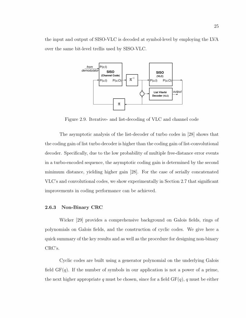
25
the input and output of SISO-VLC is decoded at symbol-level by employing the LVA
over the same bit-level trellis used by SISO-VLC.
SISO(Channel Code)
SISO(VLC)
List Viterbi Decoder (VLC)
from demodulator
output
P(u;I) P(u;O)
P(c;I)
P(u;I) P(u;O)
π
π−1
Figure 2.9. Iterative- and list-decoding of VLC and channel code
The asymptotic analysis of the list-decoder of turbo codes in [28] shows that
the coding gain of list turbo decoder is higher than the coding gain of list-convolutional
decoder. Specifically, due to the low probability of multiple free-distance error events
in a turbo-encoded sequence, the asymptotic coding gain is determined by the second
minimum distance, yielding higher gain [28]. For the case of serially concatenated
VLC’s and convolutional codes, we show experimentally in Section 2.7 that significant
improvements in coding performance can be achieved.
2.6.3 Non-Binary CRC
Wicker [29] provides a comprehensive background on Galois fields, rings of
polynomials on Galois fields, and the construction of cyclic codes. We give here a
quick summary of the key results and as well as the procedure for designing non-binary
CRC’s.
Cyclic codes are built using a generator polynomial on the underlying Galois
field GF(q). If the number of symbols in our application is not a power of a prime,
the next higher appropriate q must be chosen, since for a field GF(q), q must be either
26
a prime or a power of a prime.. Cyclic codes are built from a generator polynomial
g(X) on GF(q). The codewords are all the multiples of g(X) modulo Xn − 1, where
g(X) is a degree-r polynomial that divides Xn − 1.
CRC codes are shortened cyclic codes that can encode up to n−r information
symbols. CRC codes have excellent error detection capability. The CRC code with a
generator of degree r detects all burst errors of length r or less, and the probability
that the CRC will not detect a random error is q−r. Due to the lack of a convenient
way to calculate the error spectrum of a CRC code, ad-hoc methods have been used
for code design in the binary case.
Unfortunately the existing ad-hoc techniques for binary CRC design are not
particularly helpful for the q-ary case, but nevertheless, the general structural prop-
erties, error coverage, and burst error detection properties remain the same across
different underlying Galois fields. Therefore, even though we cannot design CRC
with specified minimum distance, still it is possible to arrive at codes that have very
respectable error detection performance. For example, for the 5-ary code used in the
next section, a reasonable choice for generator polynomial is the primitive polynomial
X8 +4X6 +X4 +X3 +X2+3X +3 which requires 8 parity symbols for data sequences
of up to 390617 symbols. The undetected codeword error probability for this code is
only 2.56 × 10⁻⁶.
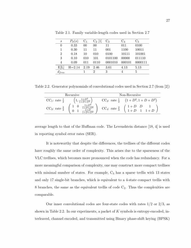
2.7 Experimental Results
Table 2.1 shows the 5-ary source used in our experiments and various codes
designed for this source. C1 is a Huffman code, C2 is a RVLC for this source reported
in [1], and the codes C3, C4, and C5 were designed by us with successively higher
redundancies. The redundancy of the VLC’s can be quantified by comparing their
27
Table 2.1. Family variable-length codes used in Section 2.7
s PS(s) C1 C2 [1] C3 C4 C5
0 0.33 00 00 11 011 01001 0.30 11 11 001 1100 100112 0.18 10 010 0100 10111 1010013 0.10 010 101 0101100 00000 0111104 0.09 011 0110 0001010 000101 0000111
E[L] H=2.14 2.19 2.46 3.61 4.13 5.13
dfree 1 2 3 4 5
Table 2.2. Generator polynomials of convolutional codes used in Section 2.7 (from [2])
Recursive Non-Recursive
CC1: rate 12
(
1, 1+D2
1+D+D2
)
CC2: rate 12
(
1 + D2, 1 + D + D2)
CC3: rate 23
(
1 0 1+D2
1+D+D2
0 1 1+D1+D+D2
)
CC4: rate 23
(
1 + D D 11 + D 1 1 + D
)
average length to that of the Huffman code. The Levenshtein distance [18, 4] is used
in reporting symbol error rates (SER).
It is noteworthy that despite the differences, the trellises of the different codes
have roughly the same order of complexity. This arises due to the sparseness of the
VLC trellises, which becomes more pronounced when the code has redundancy. For a
more meaningful comparison of complexity, one may construct more compact trellises
with minimal number of states. For example, C3 has a sparse trellis with 13 states
and only 17 single-bit branches, which is equivalent to a 4-state compact trellis with
8 branches, the same as the equivalent trellis of code C2. Thus the complexities are
comparable.
Our inner convolutional codes are four-state codes with rates 1/2 or 2/3, as
shown in Table 2.2. In our experiments, a packet of K symbols is entropy-encoded, in-
terleaved, channel encoded, and transmitted using Binary phase-shift keying (BPSK)
28
0 1 2 3 4 5 6 7 8 910−10
10−8
10−6
10−4
10−2
100
Eb/N0 (dB)
Sym
bol E
rror
Rat
e (S
ER
)
Simulation, K = 20Simulation, K = 200Bound, K = 20Bound, K = 200
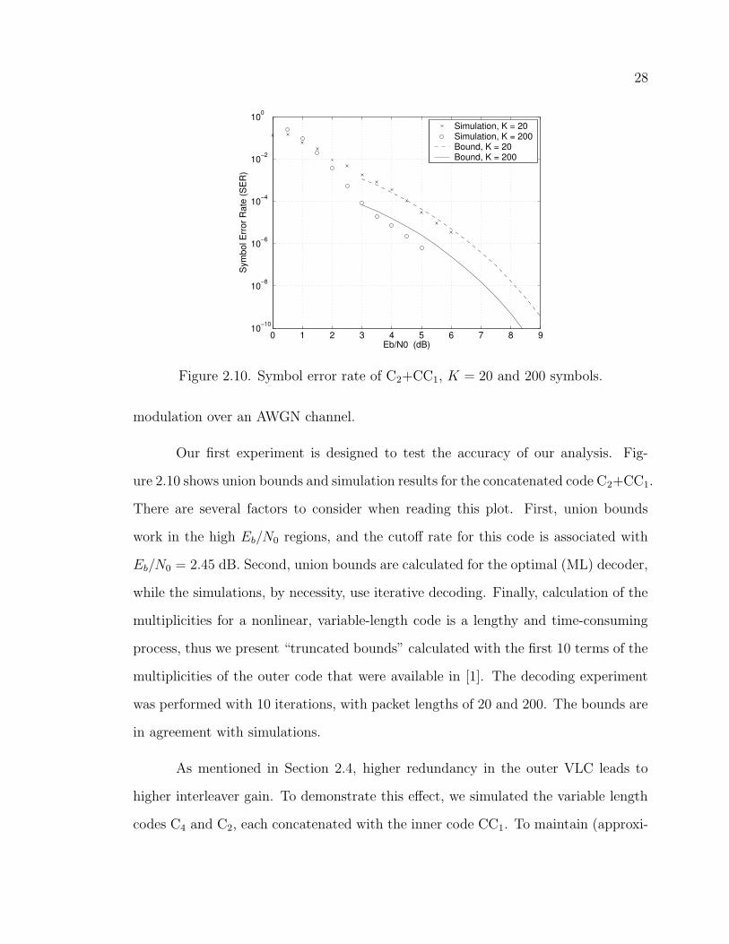
Figure 2.10. Symbol error rate of C2+CC1, K = 20 and 200 symbols.
modulation over an AWGN channel.
Our first experiment is designed to test the accuracy of our analysis. Fig-
ure 2.10 shows union bounds and simulation results for the concatenated code C2+CC1.
There are several factors to consider when reading this plot. First, union bounds
work in the high Eb/N0 regions, and the cutoff rate for this code is associated with
Eb/N0 = 2.45 dB. Second, union bounds are calculated for the optimal (ML) decoder,
while the simulations, by necessity, use iterative decoding. Finally, calculation of the
multiplicities for a nonlinear, variable-length code is a lengthy and time-consuming
process, thus we present “truncated bounds” calculated with the first 10 terms of the
multiplicities of the outer code that were available in [1]. The decoding experiment
was performed with 10 iterations, with packet lengths of 20 and 200. The bounds are
in agreement with simulations.
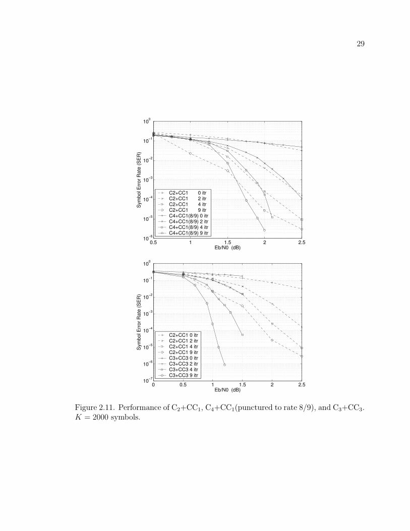
As mentioned in Section 2.4, higher redundancy in the outer VLC leads to
higher interleaver gain. To demonstrate this effect, we simulated the variable length
codes C4 and C2, each concatenated with the inner code CC1. To maintain (approxi-
29
0.5 1 1.5 2 2.510−6
10−5
10−4
10−3
10−2
10−1
100
Eb/N0 (dB)
Sym
bol E
rror
Rat
e (S
ER
)
C2+CC1 0 itrC2+CC1 2 itrC2+CC1 4 itrC2+CC1 9 itrC4+CC1(8/9) 0 itrC4+CC1(8/9) 2 itrC4+CC1(8/9) 4 itrC4+CC1(8/9) 9 itr
0 0.5 1 1.5 2 2.510−7
10−6
10−5
10−4
10−3
10−2
10−1
100
Eb/N0 (dB)
Sym
bol E
rror
Rat
e (S
ER
)
C2+CC1 0 itrC2+CC1 2 itrC2+CC1 4 itrC2+CC1 9 itrC3+CC3 0 itrC3+CC3 2 itrC3+CC3 4 itrC3+CC3 9 itr
Figure 2.11. Performance of C2+CC1, C4+CC1(punctured to rate 8/9), and C3+CC3.K = 2000 symbols.
30
0 2 4 60
1
2
3
4
5
6
7
8
9
10
SNRCCin
, SNRVLCout
SN
RC
Cou
t , S
NR
VLC
in
0 2 4 60
0.5
1
1.5
2
2.5
3
3.5
4
4.5
5
SNRCCin
, SNRVLCout
SN
RC
Cou
t , S
NR
VLC
in
CC1,Eb/N
0 = 1.05 dB
CC1,Eb/N
0 = 1.5 dB
C2
CC1(8/9),Eb/N
0 = 1.13 dB
CC1(8/9),Eb/N
0 = 1.5 dB
C4
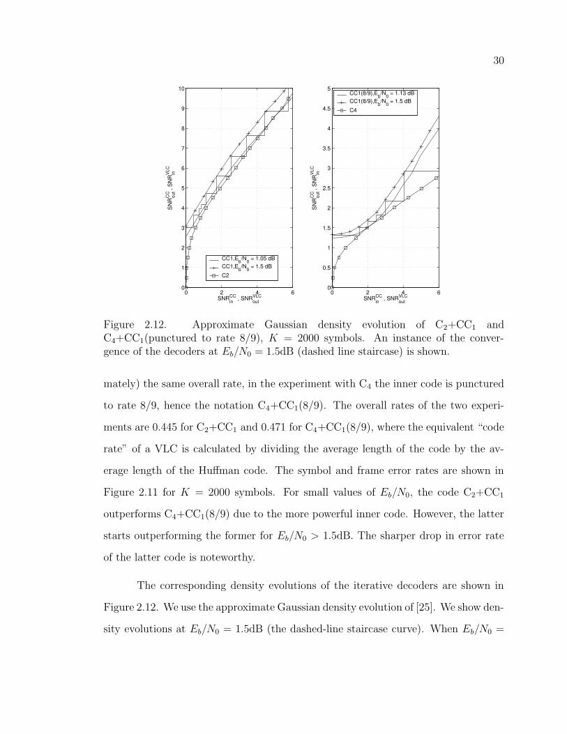
Figure 2.12. Approximate Gaussian density evolution of C2+CC1 andC4+CC1(punctured to rate 8/9), K = 2000 symbols. An instance of the conver-gence of the decoders at Eb/N0 = 1.5dB (dashed line staircase) is shown.
mately) the same overall rate, in the experiment with C4 the inner code is punctured
to rate 8/9, hence the notation C4+CC1(8/9). The overall rates of the two experi-
ments are 0.445 for C2+CC1 and 0.471 for C4+CC1(8/9), where the equivalent “code
rate” of a VLC is calculated by dividing the average length of the code by the av-
erage length of the Huffman code. The symbol and frame error rates are shown in
Figure 2.11 for K = 2000 symbols. For small values of Eb/N0, the code C2+CC1
outperforms C4+CC1(8/9) due to the more powerful inner code. However, the latter
starts outperforming the former for Eb/N0 > 1.5dB. The sharper drop in error rate
of the latter code is noteworthy.
The corresponding density evolutions of the iterative decoders are shown in
Figure 2.12. We use the approximate Gaussian density evolution of [25]. We show den-
sity evolutions at Eb/N0 = 1.5dB (the dashed-line staircase curve). When Eb/N0 =
31
0.5 1 1.5 2 2.510−4
10−3
10−2
10−1
100
Eb/N0 (dB)
Fram
e E
rror
Rat
e (F
ER
)
C2+CC1 4 itrC2+CC1 9 itrC4+CC1(8/9) 4 itrC4+CC1(8/9) 9 itrC3+CC3 4 itrC3+CC3 9 itr
Figure 2.13. FER comparison between C2+CC1, C4+CC1(punctured to rate 8/9),and C3+CC3. K = 2000 symbols.
1dB, the method predicts that neither of the codes converge. When Eb/N0 = 1.5,
both codes converge but C4+CC1(8/9) converges faster.
For further comparisons, we used the code C3 with free distance dof = 3,
concatenated with the inner code CC3, a rate 2/3 recursive convolutional code. The
concatenated code has overall rate 0.404. The SER and FER of the this code are
shown in Figure 2.11. The code C3+CC3 outperforms C2+CC1 in the entire range
of Eb/N0 after the second iteration of the decoder. The density evolutions of the
iterative decoder of C3+CC3 is shown in Figure 2.14.
As mentioned previously, Bauer and Hagenauer [1] demonstrated coding gain
via iterative source/channel decoding. But in their case the baseline system did
not have the advantage of iterative decoding. We pose a slightly different question:
assuming we have a fixed computational and rate budget, we would like to com-
pare the source/channel iterative decoder with a separable decoder whose channel
decoder is iterative. For experimental verification of this and similar questions, we
32
0 1 2 3 4 5 60
1
2
3
4
5
6
SNRCCin
, SNRVLCout
SN
RC
Cou
t , S
NR
VLC
in
CC3: E
b/N
0 = 0.5 dB
CC3: E
b/N
0 = 1.5 dB
C3
Figure 2.14. Approximate Gaussian density evolution of C3+CC3.
introduce three serial concatenated convolutional codes: SCCC1: CC2+CC1(8/9) and
SCCC2: CC4+CC3, both with overall rate 4/9, and SCCC3: CC2+CC3 with overall
rate 1/3.
We compare the iterative source/channel decoding of C2+CC1 with a system
consisting of the Huffman code C1 concatenated with SCCC2. The two systems have
the same overall rate and decoder complexity. The simulation results are not shown in
a separate figure, but one can compare the results of C2+CC1 in Figure 2.11 with the
results of C1+SCCC2 in Figure 2.15 (both for 9 iterations). The comparison indicates
that the case of separable source/channel decoding is superior to joint source/channel
decoding. We believe this is largely due to the small dfree of C2, which is the RVLC
used by Bauer and Hagenauer [1]. Therefore, it seems that separable decoding (with
an iterative channel decoder) can be superior to iterative source/channel decoding
when the outer code has small free distance.
Then one may ask: how does a joint source/channel decoder compare with
a separable decoder if we increase the free distance of the outer source code? We
33
0 0.2 0.4 0.6 0.8 1 1.2
10−6
10−5
10−4
10−3
10−2
10−1
100
Eb/N0 (dB)
Sym
bol E
rror
Rat
e (S
ER
)
C1+SCCC2 9 itrC3+CC3 9 itrC1+SCCC3 9 itrC5+CC3 9 itr
Figure 2.15. Comparison of concatenated redundant VLC and convolutional codesversus concatenated Huffman code and SCCC’s, K = 2000 symbols.
designed several experiments to address this question. In a comparison of the sepa-
rable code C1+SCCC1 with the joint source/channel decoding of C4+CC1(8/9), we
found that especially at higher Eb/N0, the joint source/channel decoding works much
better, while at intermediate Eb/N0 the two methods perform the same.
We conducted two more experiments, whose results are shown in Figure 2.15.
The separable code C1+SCCC2, is compared against C3+CC3 (both with rates ∼
4/9), where C3+CC3 outperforms C1+SCCC2 slightly. In the same Figure 2.15,
C1+SCCC3 is compared against C5+CC3 (both with rate ∼ 1/3), and they perform
roughly similarly.
Thus, the simulations did not point to a clear and universal advantage for
either the joint or separable approach. In some cases, where the outer entropy code
has low redundancy, the separable case is clearly better, while in other cases either
the joint or the separable solution might be superior. The design choices must be
made on a case-by-case basis.
34
4 5 6 7 8 910
−6
10−5
10−4
10−3
10−2
10−1
100
Eb/N0 (dB)
FER
L=1L=2L=3L=4L=5Union bound
Figure 2.16. List-decoding of C2 in AWGN channel, K=200.
2.7.1 Iterative List Decoding
We first present the performance of list-decoding of a VLC with no channel
coding. The FER of C2, with K = 200 symbols in the AWGN channel is shown in
Figure 2.16. The coding gain of the list-decoder is almost 1.1dB for L = 2, 1.5dB for
L = 3, and 1.8dB for the L = 4. The upper bound of the L = 1 case is calculated
based on the truncated union bound and the distance spectrum given in [1].
The coding gain predicted by [27] for L = 2 and L = 3 list-decoders are 1.25dB
and 1.75dB, respectively. From Figure 2.16, we observe that the predicted gains are
more than the actual gain. Using the multiplicity of the free distance of C2 provided
in [1], one can calculate the more realistic coding gain as described in Section 2.6.1.
Minor modifications may be necessary because we seek coding gain in FER and with
K = 200. The coding gain at FER=10−4 is 1dB for L = 2 and 1.4dB for L = 3. We
see that these gains better match the results of Figure 2.16.
To demonstrate the performance of the proposed iterative list-decoder, we
consider the two concatenated codes presented previously: C2+CC1 and C3+CC3.
35
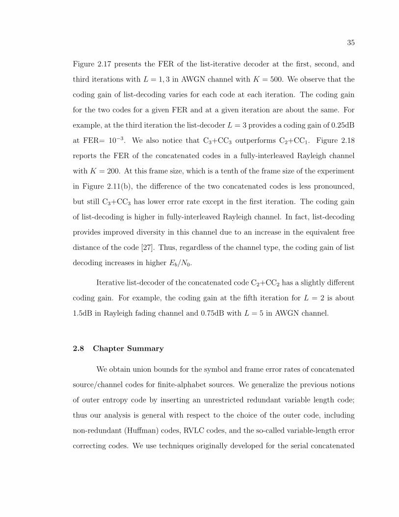
Figure 2.17 presents the FER of the list-iterative decoder at the first, second, and
third iterations with L = 1, 3 in AWGN channel with K = 500. We observe that the
coding gain of list-decoding varies for each code at each iteration. The coding gain
for the two codes for a given FER and at a given iteration are about the same. For
example, at the third iteration the list-decoder L = 3 provides a coding gain of 0.25dB
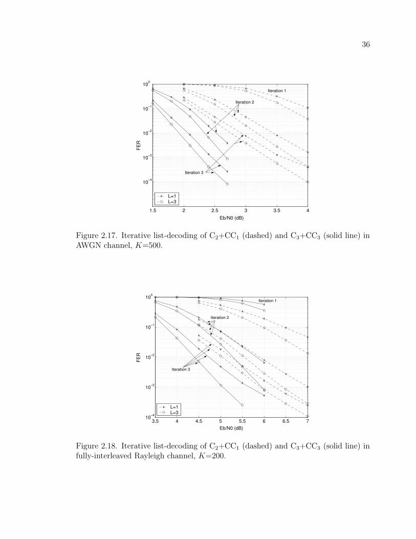
at FER= 10−3. We also notice that C3+CC3 outperforms C2+CC1. Figure 2.18
reports the FER of the concatenated codes in a fully-interleaved Rayleigh channel
with K = 200. At this frame size, which is a tenth of the frame size of the experiment
in Figure 2.11(b), the difference of the two concatenated codes is less pronounced,
but still C3+CC3 has lower error rate except in the first iteration. The coding gain
of list-decoding is higher in fully-interleaved Rayleigh channel. In fact, list-decoding
provides improved diversity in this channel due to an increase in the equivalent free
distance of the code [27]. Thus, regardless of the channel type, the coding gain of list
decoding increases in higher Eb/N0.
Iterative list-decoder of the concatenated code C2+CC2 has a slightly different
coding gain. For example, the coding gain at the fifth iteration for L = 2 is about
1.5dB in Rayleigh fading channel and 0.75dB with L = 5 in AWGN channel.
2.8 Chapter Summary
We obtain union bounds for the symbol and frame error rates of concatenated
source/channel codes for finite-alphabet sources. We generalize the previous notions
of outer entropy code by inserting an unrestricted redundant variable length code;
thus our analysis is general with respect to the choice of the outer code, including
non-redundant (Huffman) codes, RVLC codes, and the so-called variable-length error
correcting codes. We use techniques originally developed for the serial concatenated
36
1.5 2 2.5 3 3.5 4
10−4
10−3
10−2
10−1
100
Eb/N0 (dB)
FER
L=1L=3
Iteration 1
Iteration 3
Iteration 2
Figure 2.17. Iterative list-decoding of C2+CC1 (dashed) and C3+CC3 (solid line) inAWGN channel, K=500.
3.5 4 4.5 5 5.5 6 6.5 710
−4
10−3
10−2
10−1
100
Eb/N0 (dB)
FER
L=1L=3
Iteration 1
Iteration 2
Iteration 3
Figure 2.18. Iterative list-decoding of C2+CC1 (dashed) and C3+CC3 (solid line) infully-interleaved Rayleigh channel, K=200.
37
convolutional codes and adapt them so that they can be used with the nonlinear outer
codes that are of interest in source/channel coding. By evaluating the union bounds
of the concatenated scheme, we further studied the role of the constituent codes, and
illustrated through simulations the relevance of the suggested design rules.
We also propose an iterative list-decoder for VLC-based source-channel codes.
The list decoder is made possible by a non-binary CRC code which also provides
a stopping criterion for the iterative decoder. At a given iteration of the iterative
decoder, the proposed list decoder improves the overall performance of the system.
Extensive experimental results are provided in AWGN and fully-interleaved Rayleigh
channels.
CHAPTER 3
PERFORMANCE OF EQUALIZERS IN FREQUENCY-SELECTIVE
SINGLE-ANTENNA FADING CHANNELS
The performance of equalizers in fading channels is mainly characterized by di-
versity. First, we evaluate the performance and diversity order of maximum-likelihood
equalizers, and extend the results to cases with and without correlation between the
channel taps. Next, we derive the performance linear equalizers. We focus on outage
probability as a theoretical lower bound on the performance. We consider decision-
feedback equalizers as well and evaluate their performance.
3.1 Introduction
In frequency-selective fading channels, each symbol is affected by multiple
fading coefficients, providing a natural diversity to encounter the unreliable channel.
However, the inter-symbol interference makes it difficult for the receiver to exploit
this diversity.
It is known that the maximum likelihood sequence estimator (MLSE) equalizer
is able to extract the full diversity. Through pair-wise error probability and moment
generating function (MGF), we show in Section 3.2 that the maximum likelihood
(ML) detector does not prevent the receiver from achieving full diversity. We extend
the results to the case where the channel taps are correlated.
Maximum-likelihood equalizers are complex and have limited application in
practice. Linear equalizers, zero-forcing (ZF) and minimum mean square error (MMSE)
38
39
equalizers, are attractive because of their low-complexity. However, compared to ML
equalizers, linear equalizers have inferior performance and lower diversity. In Sec-
tion 3.3, we show analytically and experimentally that zero-forcing linear equalizers
are unable to harvest the available diversity in the frequency-selective channel. In
high spectral efficiency, minimum mean square linear equalizers behave the same,
however, in low spectral efficiency they are capable of achieving some of the available
diversity1.
3.2 MLSE Equalizer
In the following, we derive the error rate of MLSE equalizers in frequency-
selective SISO channels. Assume the frequency-selective channel h(D) whose taps
are symmetric complex Gaussian random variables :
h(D) = h0 + h1D + h2D2 · · · + hνD
ν
where ν represents the memory of the channel. Assuming additive white Gaussian
noise (AWGN), the transmission of L symbols over such channel results in the fol-
lowing matrix system model:
r = Hc + n
rL
rL−1...r1
=
h0 h1 · · · hν 0 · · · 00 h0 h1 · · · hν · · · 0...
. . . . . . . . . . . . . . ....
0 · · · 0 h0 h1 · · · hν
cL
cL−1...c1
+
nL
nL−1...
n1
. (3.1)
Assuming perfect knowledge about the channel taps hi’s at the receiver, the
maximum likelihood (ML) metric is given by :
m(r, c) = ||r − Hc||2 .
1The contribution of this chapter appears in part in [30].
40
An error occurs when the MLSE equalizer decides in favor of the sequence c
when the sequence c is actually transmitted. The pairwise error probability of c and
c:
Pr(c, c|H) = Q
(√
γ
2||H∆||2
)
, (3.2)
where ∆ = c − c. The unconditional pairwise error probability is
Pr(c, c) =
H (Pr(c, c, |H)) ,
and the overall error probability is the average of Pr(c, c) over all possible pairs of c
and c. Using the alternative definition of Q-function by a finite integral [31]
Q(x) =
∫ π/2
0
exp
(
− x2
2 sin2 θ
)
dθ , (3.3)
and by integrating over all channel realizations we obtain the unconditional PEP as
follows:
P (c, c) =
H (Pr(c, c, |H)) =
∫ π/2
0
ΦΓ
(
− ρ
4 sin2 θ
)
dθ (3.4)
where ΦΓ(.) is the MGF of the random variable Γ4= ||H∆||2, and ρ = Ex
N0is the
SNR. For later reference we define s4= − ρ
4 sin2 θ. We notice that the PEP is fully
expressed by the MGF of Γ. We seek this MGF for performance evaluation. Also,
the asymptotic behavior of P (c, c) is the same as asymptotic behavior of ΦΓ(.), which
determines the MLSE diversity.
The ML metric Γ = ||H∆||2 for the system model in (3.1) can be derived as
||H∆||2 = tr(H∆∆HHH) = tr(∆HHHH∆) = ∆HHHH∆ . (3.5)
Note that because of the structure of the matrix channel H in (3.1), H∆ can be
written as follows
H∆ =
h0 h1 · · · hν 0 · · · 00 h0 h1 · · · hν · · · 0...
. . . . . . . . . . . . . . ....
0 · · · 0 h0 h1 · · · hν
δL
δL−1...δ1
=
h∆L−ν
h∆L−ν+1...
h∆L
, (3.6)
41
where h = (h0, h1, · · · , hν), and ∆i4= (δi+ν , · · · , δi), a sub-vector of ∆ with length
ν + 1. Therefore, the ML metric (3.5) can be written as:
||H∆||2 =L−ν∑
i=0
∆Hi hHh∆i (3.7)
=L−ν∑
i=0
h∆i∆Hi hH = hΩhH , (3.8)
where
Ω4=
L−ν∑
i=0
∆i∆Hi (3.9)
is a square matrix with size ν + 1. The random variable Γ = hΩhH is quadratic
in the Gaussian random vector h. The following Lemma gives us the MGF of such
quadratic forms.
Lemma [32]: Let A be a Hermitian matrix and u a circularly symmetric complex
Gaussian vector with mean u and covariance matrix Ru. The MGF of the quadratic
form y = uAuH is given as
Φy(s) =
∫ ∞
0
esypY (y)dy =exp
(
−uA (I − sRuA)−1 uH)
det (I − sRuA), (3.10)
where I is the identity matrix with appropriate size.
Using above Lemma, we can obtain the MGF of Γ = hΩhH . First consider
the case where h has independent components, which leads to
ΦΓ(s) =1
det (I − sΩ)=
ν∏
i=0
(1 − sλi(Ω))−1 , (3.11)
where λi(Ω) is an eigenvalue of matrix Ω. In high SNR, ΦΓ(s) behaves as
ΦΓ(−s)·=
∏
λi(Ω)6=0
(sλi(Ω))−1 =s−(ν+1)
det(Ω), (3.12)
42
where·= expresses the asymptotic equivalence2, and for the second equality all the
eigenvalues λi(Ω) are assumed nonzero. Equation (3.12) shows that if Ω is full-rank,
the MGF, and subsequently the PEP, decays as ρ−(ν+1). Hence, the diversity order is
ν + 1.
One might ask if the maximum diversity ν + 1 is obtainable without coding.
If the vector c does not have any redundancy then c and c are different in at most
one position, hence ∆ has only one nonzero element. Let’s assume that the position
of the nonzero element of ∆ is somewhere that makes exactly ν + 1 of ∆i vectors
nonzero. Equation (3.9) shows that Ω becomes a multiple of the identity matrix,
hence has rank ν + 1. Therefore, to obtain the full frequency diversity the data need
not be redundant.
Now consider the case where h is a Gaussian vector with covariance R. One
can write h based on the white Gaussian vector h as : h = hR1
2 . Hence, the ML
metric is Γ = hR1
2ΩRH2 hH ; still a quadratic form but with a different kernel than
the previous case. The MGF is
ΦΓ(s) =1
det(
I − sR1
2ΩRH2
) =1
det (I − sRΩ)=
ν∏
i=0
(1 − sλi(RΩ))−1 . (3.13)
We notice that in this case, the matrix RΩ has the same role as Ω had in (3.11).
Therefore, as long as the covariance matrix R is full-rank, full diversity order can be
obtained. However, the correlated vector h indeed causes performance loss, but no
diversity loss. The incurred loss in performance is det(R). This can be observed in
the asymptotic behavior of ΦΓ(−s) :
ΦΓ(−s)·= det(R) det(Ω)s−(ν+1) . (3.14)
2a·= b is equivalent to a = O(b).
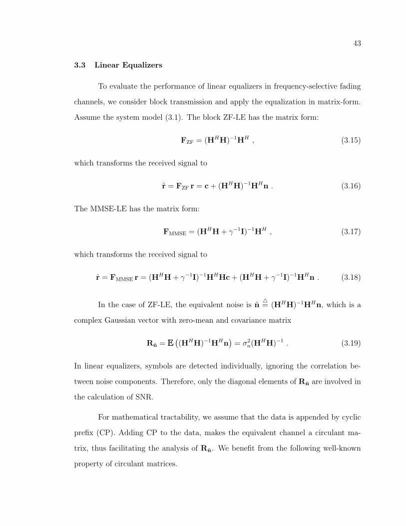
43
3.3 Linear Equalizers
To evaluate the performance of linear equalizers in frequency-selective fading
channels, we consider block transmission and apply the equalization in matrix-form.
Assume the system model (3.1). The block ZF-LE has the matrix form:
FZF = (HHH)−1HH , (3.15)
which transforms the received signal to
r = FZF r = c + (HHH)−1HHn . (3.16)
The MMSE-LE has the matrix form:
FMMSE = (HHH + γ−1I)−1HH , (3.17)
which transforms the received signal to
r = FMMSE r = (HHH + γ−1I)−1HHHc + (HHH + γ−1I)−1HHn . (3.18)
In the case of ZF-LE, the equivalent noise is n4= (HHH)−1HHn, which is a
complex Gaussian vector with zero-mean and covariance matrix
Rn = (
(HHH)−1HHn)
= σ2n(HHH)−1 . (3.19)
In linear equalizers, symbols are detected individually, ignoring the correlation be-
tween noise components. Therefore, only the diagonal elements of Rn are involved in
the calculation of SNR.
For mathematical tractability, we assume that the data is appended by cyclic
prefix (CP). Adding CP to the data, makes the equivalent channel a circulant ma-
trix, thus facilitating the analysis of Rn. We benefit from the following well-known
property of circulant matrices.
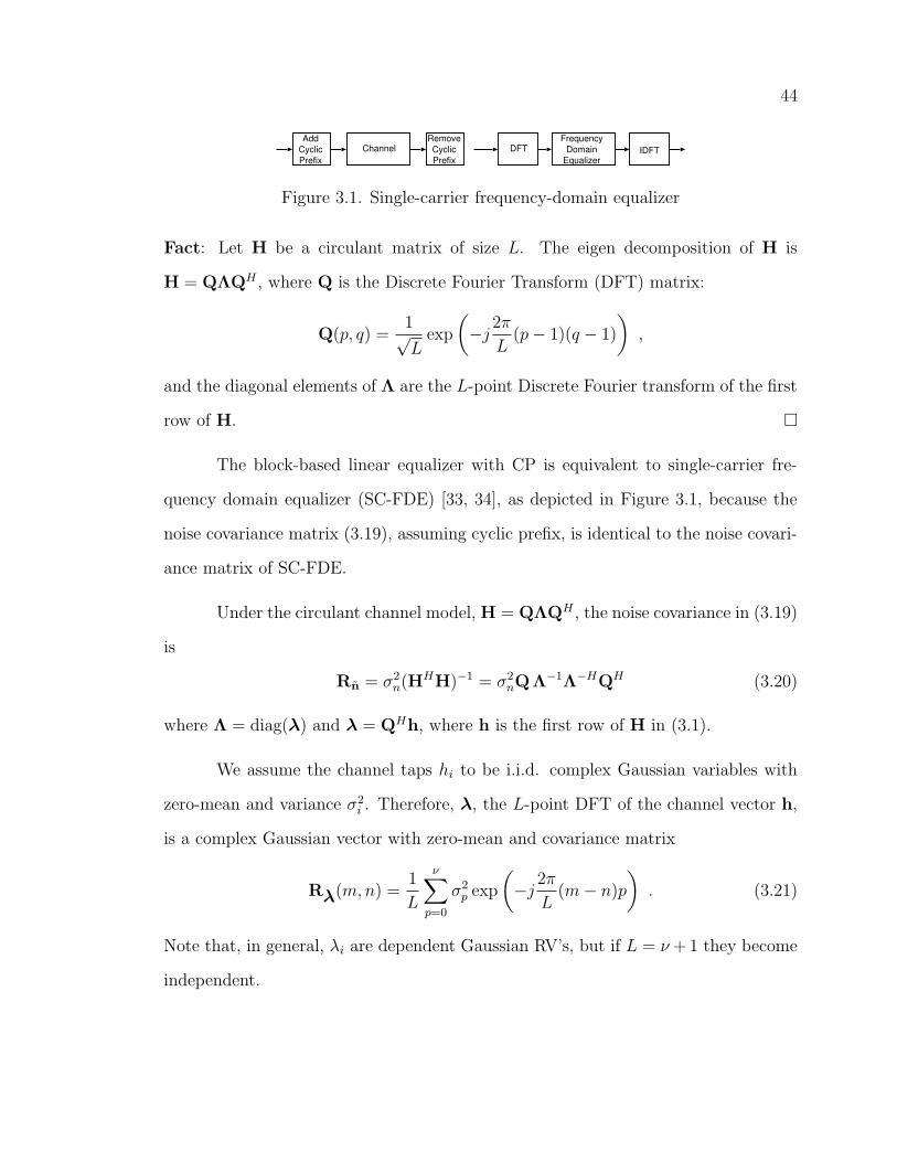
44
AddCyclicPrefix
Channel DFTFrequency
DomainEqualizer
IDFTRemoveCyclicPrefix
Figure 3.1. Single-carrier frequency-domain equalizer
Fact: Let H be a circulant matrix of size L. The eigen decomposition of H is
H = QΛQH , where Q is the Discrete Fourier Transform (DFT) matrix:
Q(p, q) =1√L
exp
(
−j2π
L(p − 1)(q − 1)
)
,
and the diagonal elements of Λ are the L-point Discrete Fourier transform of the first
row of H.
The block-based linear equalizer with CP is equivalent to single-carrier fre-
quency domain equalizer (SC-FDE) [33, 34], as depicted in Figure 3.1, because the
noise covariance matrix (3.19), assuming cyclic prefix, is identical to the noise covari-
ance matrix of SC-FDE.
Under the circulant channel model, H = QΛQH , the noise covariance in (3.19)
is
Rn = σ2n(HHH)−1 = σ2
nQΛ−1Λ−HQH (3.20)
where Λ = diag(λ) and λ = QHh, where h is the first row of H in (3.1).
We assume the channel taps hi to be i.i.d. complex Gaussian variables with
zero-mean and variance σ2i . Therefore, λ, the L-point DFT of the channel vector h,
is a complex Gaussian vector with zero-mean and covariance matrix
Rλ(m,n) =1
L
ν∑
p=0
σ2p exp
(
−j2π
L(m − n)p
)
. (3.21)
Note that, in general, λi are dependent Gaussian RV’s, but if L = ν + 1 they become
independent.
45
Evaluation of statistical expressions involving components of λ is difficult.
Multivariate Rayleigh and exponential do not in general possess a closed-form prob-
ability density function (PDF) or moment generating function (MGF) [35]. Even for
the multivariate exponential λ which is based upon a circularly symmetric Gaussian
vector, the joint PDF involves multiple integrations. In the following, to simplify
the problem, we sometimes assume that the random vector λ is an i.i.d. vector. If
ν + 1 = L the noise covariance (3.21) is indeed diagonal, therefore λ is i.i.d. If ν is
large enough, the off-diagonal elements are negligible.
Our objective is to calculate the asymptotic behavior and diversity order of
the linear equalizers. The system model (3.1) shows that the diversity order is the
same for ν + 1 = L and ν + 1 6= L. This observation comes from the fact that for
both cases each symbol is affected by exactly ν + 1 fading coefficients. Therefore, for
analytical studies, we assume ν +1 = L where λ has independent components. Later
we present experimental results that indicate our analytical findings are also valid for
ν + 1 6= L.
As a result of the independence assumption, the multivariate exponential ran-
dom vector X, defined as Xi4= |λi|2, has PDF:
f(X1, · · · , XL) =exp
(
−∑L
k=1Xk
2σ2k
)
∏Lk=1 2σ2
k
. (3.22)
In the following we provide the statistics of the decision-point signal-to-interference-
and-noise ratio (SINR) of ZF-LE and MMSE-LE.
SINR of ZF-LE
As seen in (3.16), ZF-LE cancels the interference fully. Hence, the SINR is
equal to SNR.
46
The equivalent noise of ZF-LE output is correlated. Applying the symbol-by-
symbol detection, the correlation between noise components is ignored, and only the
diagonal elements of Rn are involved in SNR calculation. Substituting Q in (3.20),
we have
Rn(i, i) =σ2
n
L
L∑
k=1
|Λ(k, k)|−2 =σ2
n
L
L∑
k=1
|λk|−2 , (3.23)
where σ2n is the AWGN variance. Since the diagonal elements of Rn are equal, the
decision-point SNR’s of all symbols are also equal and determined by the random
variable
γ =ρ
1L
L∑
k=1
|λk|−2
, (3.24)
where ρ = Ex
σ2n
is the signal to noise ratio. The decision-point SNR in (3.24) is the
harmonic average of |λk|2, k = 1, · · · , L. We evaluate the statistics of γ as follows.
Let X be an exponential random variable with variance 2σ2, and PDF fX(x) =
12σ2 exp
(
− x2σ2
)
. The MGF of Y = X−1 is
ΦY (−s) =
∫ ∞
0
esyfY (y) =
∫ ∞
0
esx fX(x)
=
√
2s
σ2K1
(
√
2s
σ2
)
, (3.25)
where Km(·) is the m-th order modified Bessel function of the second kind [36, 37].
In evaluating (3.25), we have used Equation (3.471.9) in [37] which is reported here
for convenience:
∫ ∞
0
xm−1 exp
(
− b
x− cx
)
dx = 2
(
b
c
)m/2
Km
(
2√
bc)
. (3.26)
Using (3.25), the MGF of Z = 1L
∑Li=1 X−1
i (arithmetic mean of inverse of L
independent exponential random variables) is
ΦZ(−s) =
(
2s
Lσ2
)L2
KL1
(
√
2s
Lσ2
)
. (3.27)
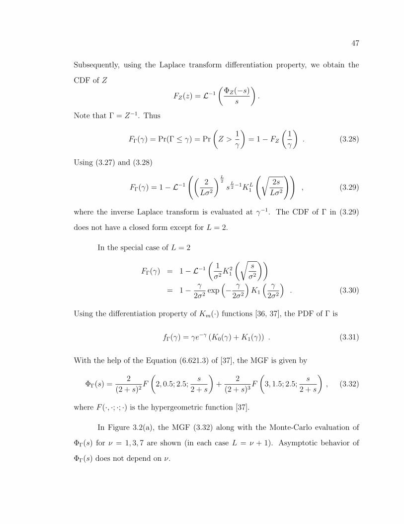
47
Subsequently, using the Laplace transform differentiation property, we obtain the
CDF of Z
FZ(z) = L−1
(
ΦZ(−s)
s
)
.
Note that Γ = Z−1. Thus
FΓ(γ) = Pr(Γ ≤ γ) = Pr
(
Z >1
γ
)
= 1 − FZ
(
1
γ
)
. (3.28)
Using (3.27) and (3.28)
FΓ(γ) = 1 − L−1
(
(
2
Lσ2
)L2
sL2−1KL
1
(
√
2s
Lσ2
))
, (3.29)
where the inverse Laplace transform is evaluated at γ−1. The CDF of Γ in (3.29)
does not have a closed form except for L = 2.
In the special case of L = 2
FΓ(γ) = 1 − L−1
(
1
σ2K2
1
(√
s
σ2
))
= 1 − γ
2σ2exp
(
− γ
2σ2
)
K1
( γ
2σ2
)
. (3.30)
Using the differentiation property of Km(·) functions [36, 37], the PDF of Γ is
fΓ(γ) = γe−γ (K0(γ) + K1(γ)) . (3.31)
With the help of the Equation (6.621.3) of [37], the MGF is given by
ΦΓ(s) =2
(2 + s)2F
(
2, 0.5; 2.5;s
2 + s
)
+2
(2 + s)3F
(
3, 1.5; 2.5;s
2 + s
)
, (3.32)
where F (·, ·; ·; ·) is the hypergeometric function [37].
In Figure 3.2(a), the MGF (3.32) along with the Monte-Carlo evaluation of
ΦΓ(s) for ν = 1, 3, 7 are shown (in each case L = ν + 1). Asymptotic behavior of
ΦΓ(s) does not depend on ν.
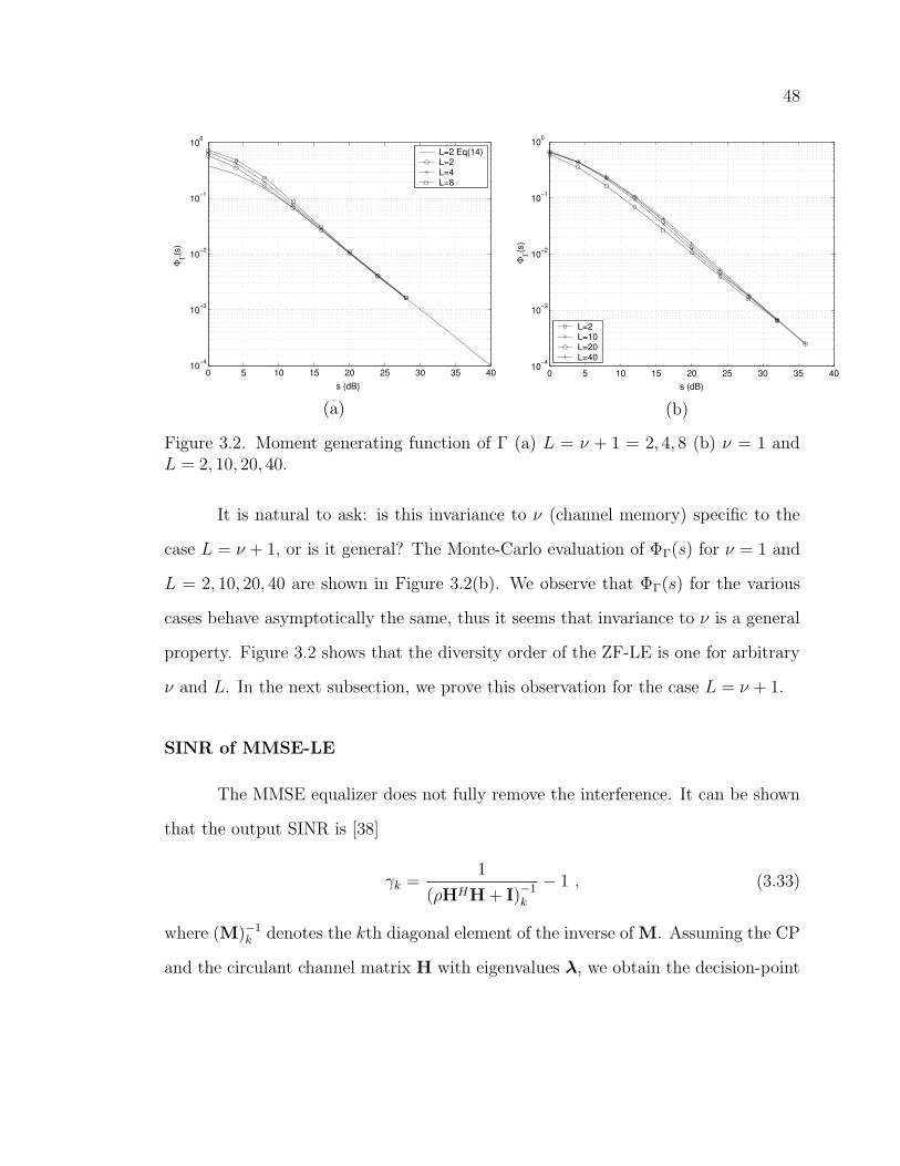
48
0 5 10 15 20 25 30 35 4010
−4
10−3
10−2
10−1
100
s (dB)
ΦΓ(s
)
L=2 Eq(14)L=2L=4L=8
(a)
0 5 10 15 20 25 30 35 4010
−4
10−3
10−2
10−1
100
L=2L=10L=20L=40
s (dB)
ΦΓ(s
)
(b)
Figure 3.2. Moment generating function of Γ (a) L = ν + 1 = 2, 4, 8 (b) ν = 1 andL = 2, 10, 20, 40.
It is natural to ask: is this invariance to ν (channel memory) specific to the
case L = ν + 1, or is it general? The Monte-Carlo evaluation of ΦΓ(s) for ν = 1 and
L = 2, 10, 20, 40 are shown in Figure 3.2(b). We observe that ΦΓ(s) for the various
cases behave asymptotically the same, thus it seems that invariance to ν is a general
property. Figure 3.2 shows that the diversity order of the ZF-LE is one for arbitrary
ν and L. In the next subsection, we prove this observation for the case L = ν + 1.
SINR of MMSE-LE
The MMSE equalizer does not fully remove the interference. It can be shown
that the output SINR is [38]
γk =1
(ρHHH + I)−1k
− 1 , (3.33)
where (M)−1k denotes the kth diagonal element of the inverse of M. Assuming the CP
and the circulant channel matrix H with eigenvalues λ, we obtain the decision-point
49
SINR as
γ =L
L∑
k=1
11+ρ|λk|2
− 1 , (3.34)
which is the same for all k’s. The harmonic average of the random variables 1+ρ|λk|2
is seen in (3.34).
Even the limited development that is provided for the statistics of the SINR
in the case of ZF-LE is not possible for MMSE-LE, because the additive term in 1 +
ρ|λk|2 makes the respective integrals intractable. Thus we resort to outage probability
analysis to show the performance of MMSE-LE.
3.3.1 Outage Probability of Linear Equalizers
The mutual information between the transmitted vector c and the linearly
processed received vector r in (3.16) and (3.18) is equal to the weighted sum of the
mutual information of their components
I(c; r) =1
L
L∑
k=1
I(ck; rk) =1
L
L∑
k=1
log(1 + γk) . (3.35)
In a circulant channel matrix H, the SINR of all symbols are the same and we have
I(c; r) = log(1 + γ). The outage occurs when the mutual information falls below a
target rate R:
Pr(O) = Pr (I(c; r) < R) = Pr (log(1 + γ) < R) . (3.36)
For ZF-LE, the SINR of each symbol is given by (3.24) which leads to
Pr(O) = Pr
(
L∑
k=1
1
ραk
>L
2R − 1
)
, (3.37)
where αk = |λk|2, and R is in bits. For MMSE-LE, the SINR is given by (3.34) which
gives
Pr(O) = Pr
(
L∑
k=1
1
1 + ραk
> L2−R
)
. (3.38)
50
We notice the apparent similarity between the outage region of ZF-LE and MMSE-LE
in the multidimensional space of the eigenvalues λ, however, the subtle difference in
the expression of the above regions gives surprisingly different outage probability.
We consider the simple case of ν = 1, i.e. a channel with two taps.
Two-tap channel (ν = 1)
With the simplifying assumption of independent λ, the outage probability of
ZF-LE, in a two-tap channel, is equal to
Pr(O) = Pr
(
1
ρα1
+1
ρα2
>2
2R − 1
)
(3.39)
=
∫ ∞
0
e−α1
∫r α1
α1ρ−r
0
e−α2dα2 dα1 (3.40)
where r = 2R−12
. Notice that the outage region in this case is unbounded. For
example, if the channel is singular, e.g. the eigenvalue α1 = 0, regardless of the value
of α2 the ZF-LE is in outage. To continue from (3.40):
Pr(O) = 1 −∫ ∞
0
exp
(
− ρα2
ρα − r
)
dα (3.41)
= 1 − e−2rρ
ρ
∫ ∞
−r
exp
(
−z
ρ− r2
zρ
)
dz , (3.42)
which is not tractable, however, we can write
Pr(O) = 1 − e−2rρ
ρ
(∫ 0
−r
exp
(
−z
ρ− r2
zρ
)
dz + 2rK1
(
2r
ρ
))
(3.43)
where (3.26) is used in the evaluation. The integral in (3.43) can be upper and lower
bounded as follows
0 ≤∫ 0
−r
exp
(
−z
ρ− r2
zρ
)
dz ≤ r exp
(
r
ρ
)
.
The first order approximation yields 2rρ
< Pr(O) < 3rρ, indicating that the diversity
order is one.
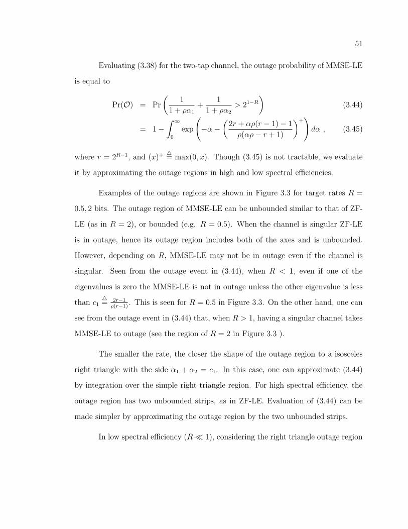
51
Evaluating (3.38) for the two-tap channel, the outage probability of MMSE-LE
is equal to
Pr(O) = Pr
(
1
1 + ρα1
+1
1 + ρα2
> 21−R
)
(3.44)
= 1 −∫ ∞
0
exp
(
−α −(
2r + αρ(r − 1) − 1
ρ(αρ − r + 1)
)+)
dα , (3.45)
where r = 2R−1, and (x)+ 4= max(0, x). Though (3.45) is not tractable, we evaluate
it by approximating the outage regions in high and low spectral efficiencies.
Examples of the outage regions are shown in Figure 3.3 for target rates R =
0.5, 2 bits. The outage region of MMSE-LE can be unbounded similar to that of ZF-
LE (as in R = 2), or bounded (e.g. R = 0.5). When the channel is singular ZF-LE
is in outage, hence its outage region includes both of the axes and is unbounded.
However, depending on R, MMSE-LE may not be in outage even if the channel is
singular. Seen from the outage event in (3.44), when R < 1, even if one of the
eigenvalues is zero the MMSE-LE is not in outage unless the other eigenvalue is less
than c14= 2r−1
ρ(r−1). This is seen for R = 0.5 in Figure 3.3. On the other hand, one can
see from the outage event in (3.44) that, when R > 1, having a singular channel takes
MMSE-LE to outage (see the region of R = 2 in Figure 3.3 ).
The smaller the rate, the closer the shape of the outage region to a isosceles
right triangle with the side α1 + α2 = c1. In this case, one can approximate (3.44)
by integration over the simple right triangle region. For high spectral efficiency, the
outage region has two unbounded strips, as in ZF-LE. Evaluation of (3.44) can be
made simpler by approximating the outage region by the two unbounded strips.
In low spectral efficiency (R 1), considering the right triangle outage region
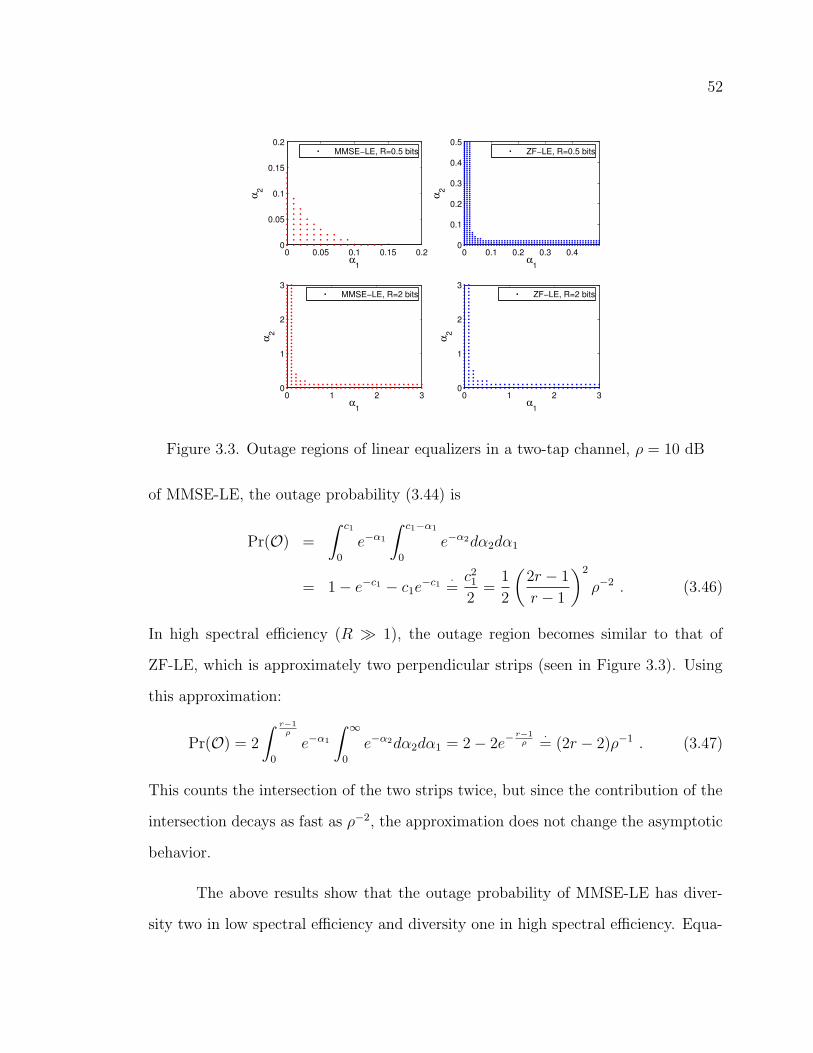
52
0 0.05 0.1 0.15 0.20
0.05
0.1
0.15
0.2
α1
α 20 0.1 0.2 0.3 0.4
0
0.1
0.2
0.3
0.4
0.5
α1
α 2
0 1 2 30
1
2
3
α1
α 2
0 1 2 30
1
2
3
α1
α 2
ZF−LE, R=0.5 bitsMMSE−LE, R=0.5 bits
ZF−LE, R=2 bitsMMSE−LE, R=2 bits
Figure 3.3. Outage regions of linear equalizers in a two-tap channel, ρ = 10 dB
of MMSE-LE, the outage probability (3.44) is
Pr(O) =
∫ c1
0
e−α1
∫ c1−α1
0
e−α2dα2dα1
= 1 − e−c1 − c1e−c1 ·
=c21
2=
1
2
(
2r − 1
r − 1
)2
ρ−2 . (3.46)
In high spectral efficiency (R 1), the outage region becomes similar to that of
ZF-LE, which is approximately two perpendicular strips (seen in Figure 3.3). Using
this approximation:
Pr(O) = 2
∫ r−1
ρ
0
e−α1
∫ ∞
0
e−α2dα2dα1 = 2 − 2e−r−1
ρ·= (2r − 2)ρ−1 . (3.47)
This counts the intersection of the two strips twice, but since the contribution of the
intersection decays as fast as ρ−2, the approximation does not change the asymptotic
behavior.
The above results show that the outage probability of MMSE-LE has diver-
sity two in low spectral efficiency and diversity one in high spectral efficiency. Equa-
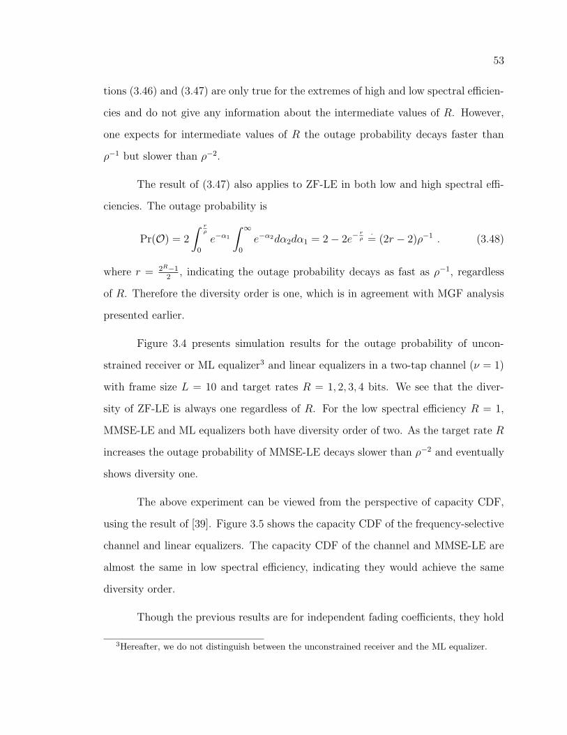
53
tions (3.46) and (3.47) are only true for the extremes of high and low spectral efficien-
cies and do not give any information about the intermediate values of R. However,
one expects for intermediate values of R the outage probability decays faster than
ρ−1 but slower than ρ−2.
The result of (3.47) also applies to ZF-LE in both low and high spectral effi-
ciencies. The outage probability is
Pr(O) = 2
∫ rρ
0
e−α1
∫ ∞
0
e−α2dα2dα1 = 2 − 2e−rρ
·= (2r − 2)ρ−1 . (3.48)
where r = 2R−12
, indicating the outage probability decays as fast as ρ−1, regardless
of R. Therefore the diversity order is one, which is in agreement with MGF analysis
presented earlier.
Figure 3.4 presents simulation results for the outage probability of uncon-
strained receiver or ML equalizer3 and linear equalizers in a two-tap channel (ν = 1)
with frame size L = 10 and target rates R = 1, 2, 3, 4 bits. We see that the diver-
sity of ZF-LE is always one regardless of R. For the low spectral efficiency R = 1,
MMSE-LE and ML equalizers both have diversity order of two. As the target rate R
increases the outage probability of MMSE-LE decays slower than ρ−2 and eventually
shows diversity one.
The above experiment can be viewed from the perspective of capacity CDF,
using the result of [39]. Figure 3.5 shows the capacity CDF of the frequency-selective
channel and linear equalizers. The capacity CDF of the channel and MMSE-LE are
almost the same in low spectral efficiency, indicating they would achieve the same
diversity order.
Though the previous results are for independent fading coefficients, they hold
3Hereafter, we do not distinguish between the unconstrained receiver and the ML equalizer.
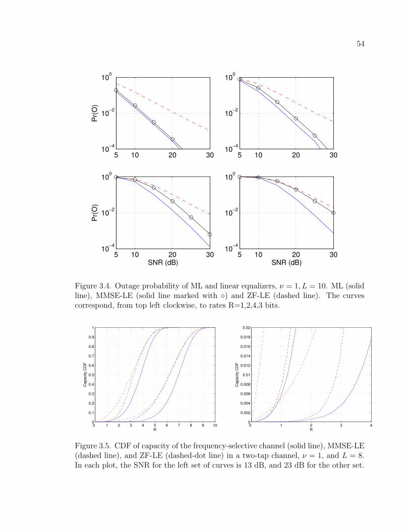
54
5 10 20 3010−4
10−2
100
Pr(
O)
5 10 20 3010−4
10−2
100
5 10 20 3010−4
10−2
100
SNR (dB)
Pr(
O)
5 10 20 3010−4
10−2
100
SNR (dB)
Figure 3.4. Outage probability of ML and linear equalizers, ν = 1, L = 10. ML (solidline), MMSE-LE (solid line marked with ) and ZF-LE (dashed line). The curvescorrespond, from top left clockwise, to rates R=1,2,4,3 bits.
0 1 2 3 4 5 6 7 8 9 100
0.1
0.2
0.3
0.4
0.5
0.6
0.7
0.8
0.9
1
R
Cap
acity
CD
F
0 1 2 3 40
0.002
0.004
0.006
0.008
0.01
0.012
0.014
0.016
0.018
0.02
R
Cap
acity
CD
F
Figure 3.5. CDF of capacity of the frequency-selective channel (solid line), MMSE-LE(dashed line), and ZF-LE (dashed-dot line) in a two-tap channel, ν = 1, and L = 8.In each plot, the SNR for the left set of curves is 13 dB, and 23 dB for the other set.
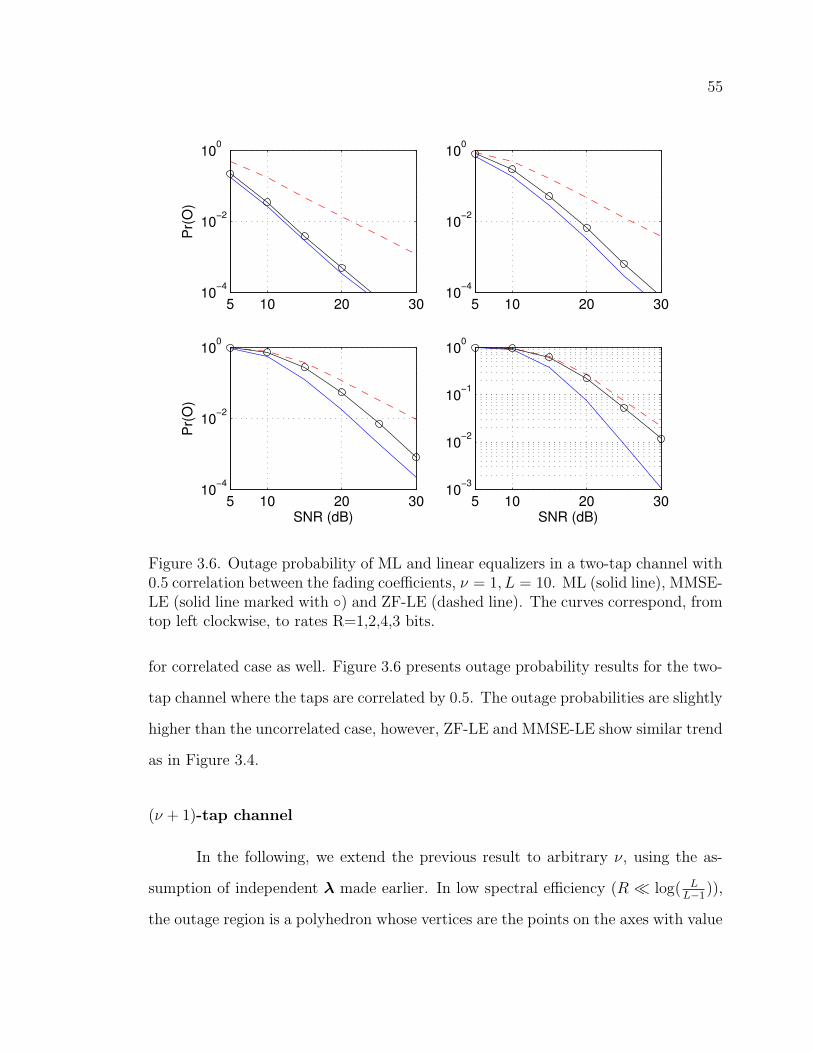
55
5 10 20 3010−4
10−2
100
Pr(
O)
5 10 20 3010−4
10−2
100
5 10 20 3010−4
10−2
100
SNR (dB)
Pr(
O)
5 10 20 3010−3
10−2
10−1
100
SNR (dB)
Figure 3.6. Outage probability of ML and linear equalizers in a two-tap channel with0.5 correlation between the fading coefficients, ν = 1, L = 10. ML (solid line), MMSE-LE (solid line marked with ) and ZF-LE (dashed line). The curves correspond, fromtop left clockwise, to rates R=1,2,4,3 bits.
for correlated case as well. Figure 3.6 presents outage probability results for the two-
tap channel where the taps are correlated by 0.5. The outage probabilities are slightly
higher than the uncorrelated case, however, ZF-LE and MMSE-LE show similar trend
as in Figure 3.4.
(ν + 1)-tap channel
In the following, we extend the previous result to arbitrary ν, using the as-
sumption of independent λ made earlier. In low spectral efficiency (R log( LL−1
)),
the outage region is a polyhedron whose vertices are the points on the axes with value
56
cν , i.e. the bounded region in the positive cone separated by the plane∑ν+1
k=1 αk = cν
where
cν4=
r(ν + 1) − 1
ρ(1 − rν),
and r4= 2R/L. The outage probability (3.38) is therefore
Pr(O) =
∫ cν−d1
0
e−α1
∫ cν−d2
0
e−α2 · · · e−αν
∫ cν−dν+1
0
e−αν+1 dαν+1 · · · dα2 dα1 , (3.49)
where di =∑i−1
j=1 αj and d1 = 0.
Pr(O) = 1 − e−cν
ν∑
k=0
ckν
k!
= 1 − e−cν
(
ecν −∞∑
k=ν+1
ckν
k!
)
·=
cν+1ν
(ν + 1)!
=
(
r(ν + 1) − 1
1 − rν
)ν+1
· ρ−(ν+1)
(ν + 1)!, (3.50)
which shows that in low spectral efficiency, the diversity order is ν + 1, the same as
that of the ML equalizer.
In high spectral efficiency (R log( LL−1
)), where the outage region of MMSE-
LE and ZF-LE become similar, we approximate the outage region as follows. The
outage event consists of ν +1 regions where the ith region, i = 1, · · · , ν +1, is defined
as 0 ≤ αi ≤ r−1ρ
, and for k 6= i, 0 ≤ αk. Extending the result of the two-tap channel,
the outage probability (3.38) is equal to
Pr(O) = (ν + 1)
∫ r−1
ρ
0
e−α1dα1
ν+1∏
i=2
∫ ∞
0
e−αidαi
= (ν + 1)(
1 − e−r−1
ρ
)
·= (ν + 1)(r − 1)ρ−1 , (3.51)
57
where, again, the intersection of the above mentioned regions is counted ν + 1 times
but this does not change the asymptotic behavior of the linearly-decaying outage
probability.
The same approximation of the outage region of MMSE-LE, in high spectral
efficiency, is applicable for ZF-LE for all values of R. With appropriate changes
in (3.51) one can conclude that the outage probability of ZF-LE decays as fast as ρ−1
regardless of R.
Figure 3.7 shows the outage probability of the ML and linear receivers for a
channel with three taps, ν = 2, frame size L = 10, and outage rates R = 1, 2, 3, 5 bits.
Similar to the results of the two-tap channel in Figure 3.4, the outage probability of
MMSE-LE has variable diversity order depending on R. In low spectral efficiency,
R = 1 in Figure 3.7, MMSE-LE has diversity order three, the same as that of ML
receiver. In high spectral efficiency, e.g. R = 5, MMSE-LE and ZF-LE show the
same diversity order one. In intermediate spectral efficiencies, the diversity order of
MMSE-LE is less than three but larger than one.
CDF of SINR
In addition to ΦΓ(s), the behavior of the CDF of Γ around zero predicts the
diversity order. The finding of [39] states if FΓ(γ) = cγd + o(γd) as γ → 0+, then at
high SNR the average error rate decays as fast as γ−d.
The CDF of γ of ZF-LE, given by in (3.24), is calculated as follows:
FΓ(γ) = Pr (Γ ≤ γ) = Pr
(
L∑
k=1
1
αk
≥ ρL
γ
)
,
which is calculated in the same way as outage probability in (3.37). Similarly, for
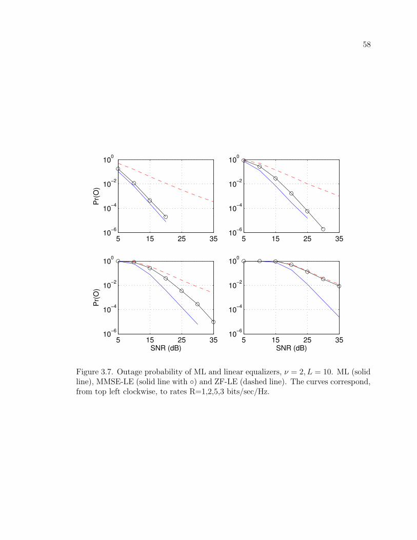
58
5 15 25 3510−6
10−4
10−2
100
Pr(
O)
5 15 25 3510−6
10−4
10−2
100
5 15 25 3510−6
10−4
10−2
100
SNR (dB)
Pr(
O)
5 15 25 3510−6
10−4
10−2
100
SNR (dB)
Figure 3.7. Outage probability of ML and linear equalizers, ν = 2, L = 10. ML (solidline), MMSE-LE (solid line with ) and ZF-LE (dashed line). The curves correspond,from top left clockwise, to rates R=1,2,5,3 bits/sec/Hz.
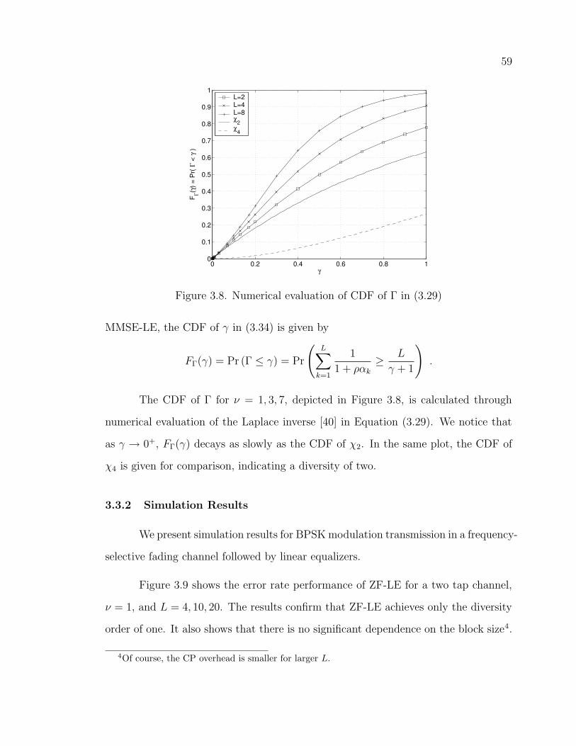
59
0 0.2 0.4 0.6 0.8 10
0.1
0.2
0.3
0.4
0.5
0.6
0.7
0.8
0.9
1
γ
F Γ(γ) =
Pr(
Γ <
γ )
L=2L=4L=8χ
2χ
4
Figure 3.8. Numerical evaluation of CDF of Γ in (3.29)
MMSE-LE, the CDF of γ in (3.34) is given by
FΓ(γ) = Pr (Γ ≤ γ) = Pr
(
L∑
k=1
1
1 + ραk
≥ L
γ + 1
)
.
The CDF of Γ for ν = 1, 3, 7, depicted in Figure 3.8, is calculated through
numerical evaluation of the Laplace inverse [40] in Equation (3.29). We notice that
as γ → 0+, FΓ(γ) decays as slowly as the CDF of χ2. In the same plot, the CDF of
χ4 is given for comparison, indicating a diversity of two.
3.3.2 Simulation Results
We present simulation results for BPSK modulation transmission in a frequency-
selective fading channel followed by linear equalizers.
Figure 3.9 shows the error rate performance of ZF-LE for a two tap channel,
ν = 1, and L = 4, 10, 20. The results confirm that ZF-LE achieves only the diversity
order of one. It also shows that there is no significant dependence on the block size4.
4Of course, the CP overhead is smaller for larger L.
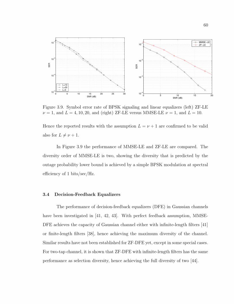
60
0 5 10 15 20 25 3010
−4
10−3
10−2
10−1
SNR (dB)
SE
R
L=10L=20L=4
0 5 10 15 2010−4
10−3
10−2
10−1
SNR (dB)
SE
R
MMSE−LEZF−LE
Figure 3.9. Symbol error rate of BPSK signaling and linear equalizers (left) ZF-LEν = 1, and L = 4, 10, 20, and (right) ZF-LE versus MMSE-LE ν = 1, and L = 10.
Hence the reported results with the assumption L = ν + 1 are confirmed to be valid
also for L 6= ν + 1.
In Figure 3.9 the performance of MMSE-LE and ZF-LE are compared. The
diversity order of MMSE-LE is two, showing the diversity that is predicted by the
outage probability lower bound is achieved by a simple BPSK modulation at spectral
efficiency of 1 bits/sec/Hz.
3.4 Decision-Feedback Equalizers
The performance of decision-feedback equalizers (DFE) in Gaussian channels
have been investigated in [41, 42, 43]. With perfect feedback assumption, MMSE-
DFE achieves the capacity of Gaussian channel either with infinite-length filters [41]
or finite-length filters [38], hence achieving the maximum diversity of the channel.
Similar results have not been established for ZF-DFE yet, except in some special cases.
For two-tap channel, it is shown that ZF-DFE with infinite-length filters has the same
performance as selection diversity, hence achieving the full diversity of two [44].
61
3.5 Chapter Summary
In this chapter, we analyze the performance of equalizers in frequency-selective
single-antenna fading channels. We present new results on the performance of linear
equalizers, and calculate their diversity order. We show that ZF-LE cannot achieve
the frequency diversity of the channel. Our analytical and experimental results show
that MMSE linear equalizers, depending on spectral efficiency, have outage probability
that decays as fast as the outage probability of unconstrained receiver, and as slowly
as that of ZF linear equalizers.
CHAPTER 4
PERFORMANCE OF EQUALIZERS IN FLAT FADING
MULTIPLE-ANTENNA CHANNELS
Multiple-input multiple output (MIMO) systems experience interference be-
tween signals transmitted simultaneously from transmit antennas. Various detection
methods can be used to retain the transmitted data. In this chapter, we consider
the performance of detection methods, also called equalizers, in flat fading MIMO
channels.
We first review the performance of ML receiver in MIMO channel and de-
velop performance bounds under spatially correlated fading. We then consider linear
receivers and calculate their outage probability. We also present results for decision-
feedback equalizers. In our derivation we consider two class of spatial encoders:
separate and joint transmit-antenna encoding.
4.1 Introduction
Consider a multiple-antenna wireless system with M transmit antennas and
N receive antennas, expressed by an N × M random matrix Ht whose elements are
i.i.d. complex Gaussian random variables. The input-output system model for flat
fading MIMO channel is
rt = Htct + nt , (4.1)
where ct is the M × 1 transmitted vector, nt ∈ CN×1 is the noise vector, and rt is
the N × 1 received vector at time instant t. In the following, the time index t is
62
63
sometimes suppressed for convenience. Equation (4.1) can be expanded to:
r1
r2...
rN
=
h1,1 h1,2 · · · h1,M
h2,1 h2,2 · · · h2,M...
.... . .
...hN,1 hN,2 · · · hN,M
c1
c2...
cM
+
n1
n2...
nN
. (4.2)
The vectors ct can be the output of two class of spatial encoders: separate and
joint spatial encoder.
Separate spatial encoding The data sequence is first demultiplexed into M sepa-
rate sub-streams. Each stream is independently channel encoded and mapped
into an appropriate signal constellation, and then transmitted from the cor-
responding antenna. Since each data symbol is sent from only one transmit
antenna, the diversity order of this scheme is at most N , the number of receive
antennas. However, this architecture provides a simple receiver. An example of
separate encoder is V-BLAST [45].
Joint spatial encoding The data stream goes under channel encoding and symbol
mapping. The stream of coded symbols is then multiplexed into M sub-streams
and each stream is transmitted from one antenna. Appropriate designs could
give the maximum diversity order of MN , but it also has a complex receiver.
Examples of joint encoding are D-BLAST [46] and space-time codes [47].
For both of the above encoding schemes, the receiver consists of an interference
cancellation module followed by an appropriate decoder. In this section, the inter-
ference cancellation module is referred to as equalizer. The equalizer performs either
linear or a non-linear process on the N received symbols. The results, M complex
variables, are the estimates of the original M transmitted symbols.
64
In this chapter, we evaluate the performance of various equalizers in flat fading
MIMO channels for both of the spatial encoders. Our evaluation excludes the channel
coding, but it can be embedded into the analysis of channel codes of choice. Moreover,
when the performance evaluation is in the form of outage probability, it gives a lower
bound on the error rate of the corresponding equalizer, presenting the error rate of
the best choice of channel codes.
4.2 Maximum Likelihood Equalizer
Consider the system model (4.1) and a block of L data vectors ct, t = 1, · · · , L
transmitted over the MIMO channel. Assuming that the receiver has perfect knowl-
edge of the channel matrix and performs coherent detection, the maximum likelihood
(ML) metric is given by m(r, c) =∑L
t=1 ||rt − Htct||2 , where r is the received signal
in the period of length L, and c is the transmitted signal in the same period.
The probability that the decoder mistakenly detects a given transmitted vector
c as c, is given by:
Pr(c, c|H) = Q
√
√
√
√
ρ
2
L∑
t=1
||Htet||2
, (4.3)
where et is the difference, at time instance t, between the transmitted vector ct and
the mistakenly detected vector ct. Using a similar procedure as in Section 3.2, we
average over H and obtain
Pr(c, c) =1
π
∫ π2
0
ΦΓ
(
− ρ
2 sin2 θ
)
dθ , (4.4)
where Γ =∑L
t=1 ||Htet||2, and ΦΓ(·) is the MGF of Γ. In a quasi-static channel,
65
where the channel Ht remains fixed over the time span of the frame, we have
Pr(c, c) =1
π
∫ π2
0
det−N(
IM − s∆∆H)
dθ
=1
π
∫ π2
0
M∏
i=1
(
1 +ρ
2 sin2 θµi
)−N
dθ (4.5)
≤M∏
i=1
(
1 +ρ
2µi
)−N
, (4.6)
where µi are the eigenvalues of ∆∆H , ∆ = [e1, . . . , eL], and s = − ρ4 sin2 θ
. Equa-
tion (4.6) is the Chernoff bound for Pr(c, c), a result which was derived differently
in [47].
In high SNR, Equation (4.6) decays like ρ−rN , where r = rank(∆∆H). There-
fore, if ∆∆H is full rank1 the ML detector achieves the diversity order of MN . To
obtain full diversity with the ML detector, ∆∆H must be full rank for all possible
pairs of transmit vectors. This is the so-called rank criterion derived in [47].
The performance of ML equalizers in a spatially correlated flat fading channel
has also been studied. A well-accepted model is to separate transmit- and receive-side
correlation [48]:
H = R1
2
TxHRH2
Rx (4.7)
where RTx is the correlation between the transmit antennas, and RRx is the correla-
tion between the receive antennas. A similar procedure as in the uncorrelated case
results in [49]:
Pr(c, c) =1
π
∫ π2
0
det−1(
IMN − s(IN ⊗ ∆∆H)(RRx ⊗ RTx))
dθ
=1
π
∫ π2
0
M∏
i=1
N∏
j=1
(
1 +ρλjµi
2 sin2 θ
)−N
dθ ≤M∏
i=1
N∏
j=1
(
1 +1
2ρλjµi
)−1
,(4.8)
1Note that if L < M then ∆∆H cannot be full rank.
66
where λj are the eigenvalues of RRx and µi are the eigenvalues of ∆∆HRTx.
High SNR approximation of (4.8) shows that the diversity order is not dimin-
ished as long as RRx and RTx are full rank.
4.3 Linear Equalizers
We consider linear equalizers and evaluate the outage probability of a flat
fading MIMO channel, with N ≥ M , followed by a ZF linear equalizer (ZF-LE) or
MMSE linear equalizer (MMSE-LE). In our treatment, we consider both separate and
joint spatial encoders.
Assume the system model (4.1): r = Hc + n. The ZF equalizer is
FZF = (HHH)−1HH (4.9)
which transforms the received signal to
r = FZF r = c + (HHH)−1HHn . (4.10)
The MMSE equalizer is
FMMSE = (HHH + ρ−1I)−1HH (4.11)
which transforms the received signal to
r = FMMSE r = (HHH + ρ−1I)−1HHHc + (HHH + ρ−1I)−1HHn . (4.12)
Since the symbols are detected individually, the SINR of the individual symbols de-
termine the performance.
67
SINR of ZF-LE
The detection noise in (4.10), n4= (HHH)−1HHn, is a complex Gaussian
vector with zero-mean and covariance matrix
Rn = (
(HHH)−1HHn)
= σ2n(HHH)−1 . (4.13)
Since the interference from other transmit antennas is completely removed by zero-
forcing, noise remains, which is characterized by the diagonal elements of Rn, given
by:
Rn(k, k) = σ2n(HHH)−1
k = σ2n
det(
HHH)
det (HHH), (4.14)
where (M)−1k represents the kth diagonal element of the inverse of M, and H is
obtained by removing the kth row of H. In the following, without loss of generality,
we assume k = 1, thus H = [h; H], the following result is applicable when k 6= 1. A
simple matrix algebra gives the following relation between the determinants involved
in (4.14):
det(
HHH)
= det(
HHH)
det(
hHh − hHPh)
,
where P4= H
(
HHH)−1
HH is an N × N matrix. Note that det(
hHh − hHPh)
=
hH(I − P)h. Substituting in (4.14) we obtain:
Rn(1, 1) =σ2
n
hH(I − P)h. (4.15)
Considering the above noise variance and the eigen decomposition I − P = QHΛQ,
we get the associated SNR
γ1 = ρhH(I − P)h = ρhHQHΛQh . (4.16)
Since h ∈ CN×1 is an i.i.d. vector, its distribution is invariant under a unitary
transformation. Therefore, h4= Qh has the same distribution as h, which results in
68
general non-central chi-square distribution for γ1 = ρhHΛh. However, considering
that P and I − P are projection matrices2, we can provide the statistics of γ1 more
specifically.
Since P is a projection matrix rank(P) = tr(P) [50], and we have
rank(P) = tr
(
H(
HHH)−1
HH
)
= M − 1 ,
which gives rank(I − P) = N − M + 1. Also, the eigenvalues of a projection matrix
are either one or zero [50]. Hence, Λ, the diagonal eigenvalue matrix of P, has only
N − M + 1 non-zero diagonal elements which are all one. This results in central
chi-square distribution with 2(N − M + 1) degrees of freedom for γ1 in (4.16).
Above procedure can be applied to obtain the same result for the SNR of other
symbols. Being the column of an i.i.d. channel matrix H, hk’s are independent which
results in the independence of γk. Therefore, the independent γk’s are chi-square
random variables with degrees 2(N − M + 1). The CDF of Y ∼ χ2(N−M+1), with
variance 0.5 for the participating Gaussian random variables, is:
FY (y) = 1 − e−y
N−M+1∑
i=1
yi−1
(i − 1)!. (4.17)
Above result has appeared in literature previously. Perhaps, the first time it
appeared in [51] in the context of multiple access interference, and recently in [52].
SINR of MMSE-LE
In MMSE detection, unlike ZF detection, the channel is not fully inverted
and there is residual interference left after linear processing. Hence, both noise and
interference determine the performance. It has been shown [38] that the SINR of the
2P is a projection matrix if P
m = P for all positive integers m.
69
kth symbol of MMSE detector is
γk = hHk
(
HkHHk + ρ−1I
)−1
hk (4.18)
=1
(I + ρHHH)−1k
− 1 , (4.19)
where hk is the kth column of the channel matrix H and removing this column from
H gives Hk ∈ CN×(M−1).
The statistics of γk in (4.18), although more complicated than the ZF case,
has been investigated in the context of additive interference channels. Reference [53]
is entirely devoted to the derivation of the CDF of the output SINR of an MMSE
detector. Consider (4.18) and remove the subscript k for simplicity. The quadratic
form Y = hHR−1h, whose kernel depends on the random matrix R4= HHH + ρ−1I
and H ∈ CN×(M−1), has the CDF
FY (y) = 1 − exp
(
−y
ρ
) N∑
n=1
An(y)
(n − 1)!
(
y
ρ
)n−1
(4.20)
where the auxiliary functions An(y) are given by
An(y) =
1 N ≥ M + n − 11+∑N−n
i=1Ciy
i
(1+y)M−1 N < M + n − 1 ., (4.21)
and Ci is the coefficient of yi in (1 + y)M−1 [53].
Note that the SINR of the various symbols, γ1, · · · , γM , are generally corre-
lated, unlike the ZF-LE case. In fact, they are negatively correlated which leads to
surprisingly different performance than ZF-LE in some rate regions.
4.3.1 Outage Probability in Separate Spatial Encoding
In separate spatial encoding, the data stream is demultiplexed to several sub-
streams, each for one transmit antenna. A simple observation in the evaluation of the
outage probability is that if any of the equivalent parallel channels is in outage, the
70
system is in outage. Hence, the outage event, O, is the event when any of the sub-
channels cannot support the rate that is assigned to it. In our analysis, we consider
equal rate for the sub-channels, however, it is also possible to have a non-uniform
rate assignment.
After linear transformation, the mutual information between the elements of
r, in (4.10) and (4.12), and the transmitted data vector c is :
I(ck; rk) = log(1 + γk) . (4.22)
Assume the target rate is R, and let L4= N − M . The outage probability Pr(O) is :
Pr(O) = 1 − Pr(Oc)
= 1 − Pr
(
I(c1; r1) ≥R
M, · · · , I(cM ; rM) ≥ R
M
)
= 1 −(
Pr
(
I(ck; rk) ≥R
M
))M
≈ M Pr
(
I(ck; rk) <R
M
)
. (4.23)
Notice that in the above derivation, we have used that fact that sub-channels outage
events are independent. This is based on the independence between the SINR of
various symbols. As we notice previously, this is a valid assumption for ZF-LE. While
this assumption does not hold for MMSE-LE, it does give a useful approximation,
providing the diversity order.
Substituting (4.17) and (4.22) in (4.23) gives the outage probability for ZF-LE
which is
Pr(O) ≈ MFY
(
2R/M − 1
ρ
)
(4.24)
= M − Me−y
(
ey −∞∑
i=L
yi−1
(i − 1)!
)∣
∣
∣
∣
∣
y= 2R/M−1
ρ
·=
M(2R/M − 1)L+1
(L + 1)!ρ−(L+1) , (4.25)
71
which shows the diversity order L + 1 for the ZF-LE.
Substituting (4.20) and (4.22) in (4.23) results in the outage probability of
MMSE-LE
Pr(O) ≈ MFY
(
2RM − 1
)
= M − Me−yρ
(
eyρ −
∞∑
i=L+1
1
k!
(
y
ρ
)i
+N∑
i=L+2
Ai(y)
(i − 1)!
(
y
ρ
)i−1)∣
∣
∣
∣
∣
y=2RM −1
(4.26)
·=
yL+1
(L + 1)!· yM−1
(1 + y)M−1ρ−(L+1)
∣
∣
∣
∣
y=2RM −1
, (4.27)
which also shows the diversity order L + 1 for the MMSE-LE, the same as that of
ZF-LE. However, the two outage probabilities are not exactly the same. The ratio of
the outage probability of (4.25) to (4.27) is the inverse of the middle term in (4.27):
Pr(O)ZF
Pr(O)MMSE
=(1 + y)M−1
yM−1
∣
∣
∣
∣
y=2RM −1
=
(
2RM
2RM − 1
)M−1
. (4.28)
Note that the ratio of outage probabilities in (4.28) remains fixed throughout
the range of SNR and it only depends on the relative target rate, RM
. When the
relative target rate is small, the outage probability of ZF-LE becomes larger than
that of MMSE-LE. When the target rate is large this difference between the outage
probabilities becomes negligible. We demonstrate this fact in the experimental results
in Section 4.3.3.
Generalization of the above results to non-uniform rate assignment is straight-
forward. Uniform and non-uniform rate assignment have the same diversity, though
they have different performance.
It is also possible to obtain the diversity-multiplexing tradeoff, introduced
in [54], for ZF-LE and MMSE-LE. In the framework of [54], the target rate is defined
for a family of codes, whose members are designed to be employed each in a given
72
SNR. A family of codes achieves the spatial multiplexing gain of r if it supports the
target rate R = r log ρ.
For ZF-LE, a similar derivation as in (4.25) leads to
Pr(O) ≈ MFY
(
ρrM − 1
ρ
)
= M − Me−y
(
ey −∞∑
i=L
yi−1
(i − 1)!
)∣
∣
∣
∣
∣
y= ρrM −1
ρ
·=
M
(L + 1)!ρ−(L+1)(1− r
M)+ , (4.29)
where (x)+ = max(0, x). The above result indicates that ZF-LE achieves the diversity
gain of d(r) = (L + 1)(1 − rM
). We notice that for a multiplexing gain of r = 0, i.e.
fixed target rate throughout the SNR region, the diversity is the same as what (4.25)
indicates. However, when the multiplexing gain increases, the diversity gain decreases
and in the limit of r = M , the maximum multiplexing gain, the diversity gain is zero.
Similarly for MMSE-LE, the derivation which led to (4.27) gives us:
Pr(O) ≈ MFY
(
ρrM − 1
)
·=
yL+1
(L + 1)!· yM−1
(1 + y)M−1ρ−(L+1)
∣
∣
∣
∣
y=ρrM −1
·=
M
(L + 1)!ρ−(L+1)(1− r
M)+ , (4.30)
which is the same diversity gain as that of ZF-LE.
4.3.2 Outage Probability in Joint Spatial Encoding
In joint spatial encoding, the data stream is encoded and then demultiplexed
into sub-streams to be sent from the antennas. Effectively, each data symbol con-
tribute to signals of all the transmit antennas. Considering the act of linear equalizers,
outage occurs when the aggregate mutual information of all the sub-channels fails to
support the target rate [38].
73
The mutual information between the elements of the linearly transformed re-
ceive signal, r in (4.10) and (4.12), and the transmitted data vector c is I(ck; rk) =
log(1 + γk). Assuming the target rate is R, the probability of the outage event O is
Pr(O) = Pr
(
M∑
k=1
I(ck; rk) < R
)
= Pr
(
M∑
k=1
log(1 + γk) < R
)
(4.31)
= Pr
(
M∏
k=1
(1 + γk) < 2R
)
. (4.32)
The SINR of the sub-channels of ZF-LE are independent chi-square random
variables with degrees 2(N−M +1). Let Yk ∼ χ2(N−M+1), k = 1, · · · ,M . The outage
probability of ZF-LE is given by the CDF of the random variable
M∏
k=1
(1 + Yk) = 1 +M∑
k=1
Yk + · · · +M∏
k=1
Yk . (4.33)
Among the components of the above random variable, the last term, which is the
product of Yk’s, determines the diversity order. In the following, through recursion,
we show that Y1 · Y2 · · ·YM has diversity order L. Let us start by Z4= Y1 · Y2. The
PDF of Z is given by
fZ(z) =2
((L − 1)!)2zLK0
(
2√
z)
, (4.34)
where K0(·) is the zeroth order modified Bessel function of the second kind [36], which
for small values of z is a constant3. Therefore, for small values of z the first order
approximation of fZ(z) is zL. This shows that the CDF of Z, FZ(z), has first order
approximation equal to zL+1, which indicates diversity order of L + 1. Now consider
3For small values of x: Km(x) ∼ Γ(m)2 (2/x)m [37].
74
the CDF of W4= Y1 · Y2 · Y3 = Z · Y , where Y ∼ χ2(N−M+1):
FW (w) = Pr(W ≤ w) = Pr(Z · Y ≤ w) =
∫ ∞
0
fZ(z)FY (w
z)dz
=
∫ ∞
0
αzLK0
(
2√
z)
(
1 − e−wz
L+1∑
k=1
wk−1
zk−1(k − 1)!
)
dz
= α
∫ ∞
0
zLK0
(
2√
z)
e−wz
∞∑
k=L+2
wk−1
zk−1(k − 1)!dz , (4.35)
where α is the constant term in (4.34). The first order approximation of (4.35) around
zero is
wL+1
∫ ∞
0
α
z(L + 1)!K0
(
2√
z)
dz .
Thus FW (w) behaves like the L+1th power of w, indicating the diversity order L+1.
This procedure can be applied recursively to find that the first order approximation
of the CDF of Y1 · Y2 · · ·YM behaves like wL+1. As mentioned, the product term,
among the ones in (4.33), dominates the diversity. We just showed that the product
term Y1 · Y2 · · ·YM has the diversity order L + 1. Therefore, the diversity order of
ZF-LE is L + 1.
Recalling the results from Section 4.3.1, ZF-LE has the same diversity in joint
and separate spatial encoding architecture.
To obtain the outage probability of MMSE-LE, we substitute the SINR of
MMSE-LE from (4.19) in (4.32) which gives:
Pr(O) = Pr
(
M∏
k=1
(
I + ρHHH)−1
k> 2−R
)
. (4.36)
The involvement of the diagonal elements of the random matrix(
I + ρHHH)−1
makes
further analysis intractable. We proceed to provide an upper bound to this probabil-
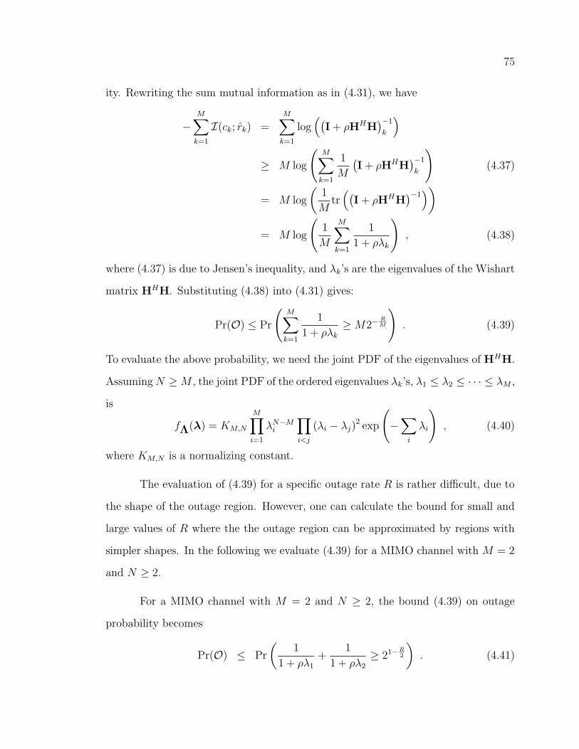
75
ity. Rewriting the sum mutual information as in (4.31), we have
−M∑
k=1
I(ck; rk) =M∑
k=1
log(
(
I + ρHHH)−1
k
)
≥ M log
(
M∑
k=1
1
M
(
I + ρHHH)−1
k
)
(4.37)
= M log
(
1
Mtr(
(
I + ρHHH)−1)
)
= M log
(
1
M
M∑
k=1
1
1 + ρλk
)
, (4.38)
where (4.37) is due to Jensen’s inequality, and λk’s are the eigenvalues of the Wishart
matrix HHH. Substituting (4.38) into (4.31) gives:
Pr(O) ≤ Pr
(
M∑
k=1
1
1 + ρλk
≥ M2−RM
)
. (4.39)
To evaluate the above probability, we need the joint PDF of the eigenvalues of HHH.
Assuming N ≥ M , the joint PDF of the ordered eigenvalues λk’s, λ1 ≤ λ2 ≤ · · · ≤ λM ,
is
fΛ(λ) = KM,N
M∏
i=1
λN−Mi
∏
i<j
(λi − λj)2 exp
(
−∑
i
λi
)
, (4.40)
where KM,N is a normalizing constant.
The evaluation of (4.39) for a specific outage rate R is rather difficult, due to
the shape of the outage region. However, one can calculate the bound for small and
large values of R where the the outage region can be approximated by regions with
simpler shapes. In the following we evaluate (4.39) for a MIMO channel with M = 2
and N ≥ 2.
For a MIMO channel with M = 2 and N ≥ 2, the bound (4.39) on outage
probability becomes
Pr(O) ≤ Pr
(
1
1 + ρλ1
+1
1 + ρλ2
≥ 21−R2
)
. (4.41)
76
For small values of R, the outage region is a isosceles right triangle with the side
λ1 + λ2 = c2, where c24= 2−b
ρ(b−1)and b
4= 21−R
2 . When M = N = 2, above outage
probability bound, up to the scaling factor K2,2, is
Pr(O) ≤∫ c2
0
e−λ1
∫ c2−λ1
0
(λ1 − λ2)2e−λ2dλ2 dλ1
= 2
(
1 − e−c2
(
1 + c2 +c22
2+
c32
6
))
= 2e−c2
∞∑
k=4
ck2
k!
·=
1
12c42 =
1
12
(
2 − b
b − 1
)4
ρ−4 , (4.42)
which indicates diversity four. When N ≥ 2 the outage probability bound (4.39), up
to the scaling factor K2,N , is
Pr(O) ≤∫ c2
0
e−λ1λN−21
∫ c2−λ1
0
λN−22 (λ1 − λ2)
2e−λ2dλ2 dλ1
= 2(N − 1)!(N − 2)!
(
1 − e−c2
2N−1∑
k=1
ck2
k!
)
·=
2(N − 1)!(N − 2)!
(2N)!
(
2 − b
b − 1
)2N
ρ−2N , (4.43)
where the achieved diversity is 2N . In obtaining (4.42) and (4.43), the following
identities are helpful:
∫ u
0
xne−xdx = n! − e−u
n∑
k=0
n!
(n − k)!un−k ,
∫ u
0
xn(u − x)mdx = um+n+1B(m + 1, n + 1) ,
where m and n are integers and B(·, ·) is the Beta function which is B(b, c) =
Γ(b)Γ(c)Γ(b+c)
[37], and Γ(·) denotes the Gamma function.
For large values of R, the outage region is approximated by two orthogonal
strips. The strips are defined as 0 ≤ λ2, 0 ≤ λ1 ≤ c2 and 0 ≤ λ1, 0 ≤ λ2 ≤ c2, where
77
c24= 1−b
bρ. The outage probability bound, up to the scaling factor K2,N , is
Pr(O) ≤ 2
∫ c2
0
e−λ1λN−21
∫ ∞
0
λN−22 (λ1 − λ2)
2e−λ2dλ2 dλ1
= 4(N − 1)! (N − 2)! e−c2
∞∑
k=N−1
xk
k!
+2(N − 2)! e−c2(
(N − 2)cN−12 − cN
2
)
·= 2N(N − 2)! cN−1
2
= 2N(N − 2)!
(
1 − b
b
)N−1
ρ−(N−1) , (4.44)
which indicates that the upper bound4 has the diversity N − 1 = L + 1, where
L = N − M as introduced previously. In the calculation of (4.44), the intersection
of the two strips is calculated twice. This portion of integral, which decays as fast as
ρ−2(N−1), does not affect the asymptotic behavior of (4.44).
The upper bounds in (4.42) and (4.43) show the surprising fact that MMSE-
LE can achieve the same diversity as the ML receiver for small values of R in joint
spatial encoding. However, for large values of R the performance of MMSE-LE and
ZF-LE are the same. Hence, the diversity of MMSE-LE varies from the full diversity
of an unconstrained detector to that of ZF-LE, depending of the target rate R.
Comparing to the results from Section 4.3.1 for separate spatial encoders,
MMSE-LE has different diversity in joint spatial encoding architecture, except for
large outage rate R.
The previous results of the case M = 2, N ≥ 2 can be generalized to arbitrary
values of M and N ≥ M .
4In Section 4.3.3 is shown that the upper bound is tight in high spectral efficiency region.
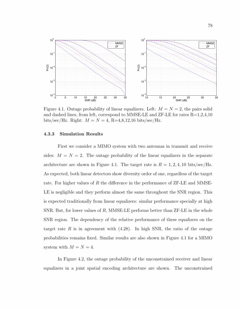
78
0 5 10 15 20 25 30 3510
−4
10−3
10−2
10−1
100
SNR (dB)
Pr(
O)
MMSEZF
10 15 20 25 30 3510
−4
10−3
10−2
10−1
100
SNR (dB)
Pr(
O)
MMSEZF
Figure 4.1. Outage probability of linear equalizers. Left: M = N = 2, the pairs solidand dashed lines, from left, correspond to MMSE-LE and ZF-LE for rates R=1,2,4,10bits/sec/Hz. Right: M = N = 4, R=4,8,12,16 bits/sec/Hz.
4.3.3 Simulation Results
First we consider a MIMO system with two antennas in transmit and receive
sides: M = N = 2. The outage probability of the linear equalizers in the separate
architecture are shown in Figure 4.1. The target rate is R = 1, 2, 4, 10 bits/sec/Hz.
As expected, both linear detectors show diversity order of one, regardless of the target
rate. For higher values of R the difference in the performance of ZF-LE and MMSE-
LE is negligible and they perform almost the same throughout the SNR region. This
is expected traditionally from linear equalizers: similar performance specially at high
SNR. But, for lower values of R, MMSE-LE performs better than ZF-LE in the whole
SNR region. The dependency of the relative performance of these equalizers on the
target rate R is in agreement with (4.28). In high SNR, the ratio of the outage
probabilities remains fixed. Similar results are also shown in Figure 4.1 for a MIMO
system with M = N = 4.
In Figure 4.2, the outage probability of the unconstrained receiver and linear
equalizers in a joint spatial encoding architecture are shown. The unconstrained
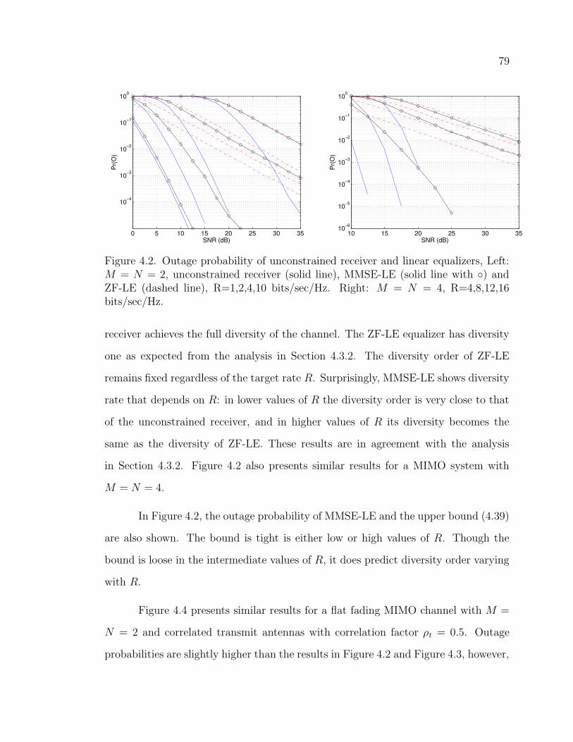
79
0 5 10 15 20 25 30 35
10−4
10−3
10−2
10−1
100
SNR (dB)
Pr(
O)
10 15 20 25 30 3510
−6
10−5
10−4
10−3
10−2
10−1
100
SNR (dB)
Pr(
O)
Figure 4.2. Outage probability of unconstrained receiver and linear equalizers, Left:M = N = 2, unconstrained receiver (solid line), MMSE-LE (solid line with ) andZF-LE (dashed line), R=1,2,4,10 bits/sec/Hz. Right: M = N = 4, R=4,8,12,16bits/sec/Hz.
receiver achieves the full diversity of the channel. The ZF-LE equalizer has diversity
one as expected from the analysis in Section 4.3.2. The diversity order of ZF-LE
remains fixed regardless of the target rate R. Surprisingly, MMSE-LE shows diversity
rate that depends on R: in lower values of R the diversity order is very close to that
of the unconstrained receiver, and in higher values of R its diversity becomes the
same as the diversity of ZF-LE. These results are in agreement with the analysis
in Section 4.3.2. Figure 4.2 also presents similar results for a MIMO system with
M = N = 4.
In Figure 4.2, the outage probability of MMSE-LE and the upper bound (4.39)
are also shown. The bound is tight is either low or high values of R. Though the
bound is loose in the intermediate values of R, it does predict diversity order varying
with R.
Figure 4.4 presents similar results for a flat fading MIMO channel with M =
N = 2 and correlated transmit antennas with correlation factor ρt = 0.5. Outage
probabilities are slightly higher than the results in Figure 4.2 and Figure 4.3, however,
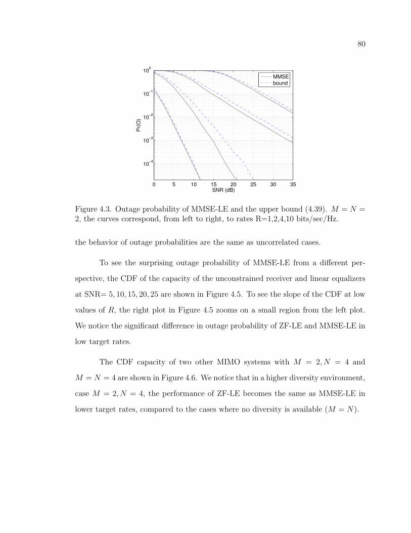
80
0 5 10 15 20 25 30 35
10−4
10−3
10−2
10−1
100
SNR (dB)
Pr(
O)
MMSEbound
Figure 4.3. Outage probability of MMSE-LE and the upper bound (4.39). M = N =2, the curves correspond, from left to right, to rates R=1,2,4,10 bits/sec/Hz.
the behavior of outage probabilities are the same as uncorrelated cases.
To see the surprising outage probability of MMSE-LE from a different per-
spective, the CDF of the capacity of the unconstrained receiver and linear equalizers
at SNR= 5, 10, 15, 20, 25 are shown in Figure 4.5. To see the slope of the CDF at low
values of R, the right plot in Figure 4.5 zooms on a small region from the left plot.
We notice the significant difference in outage probability of ZF-LE and MMSE-LE in
low target rates.
The CDF capacity of two other MIMO systems with M = 2, N = 4 and
M = N = 4 are shown in Figure 4.6. We notice that in a higher diversity environment,
case M = 2, N = 4, the performance of ZF-LE becomes the same as MMSE-LE in
lower target rates, compared to the cases where no diversity is available (M = N).
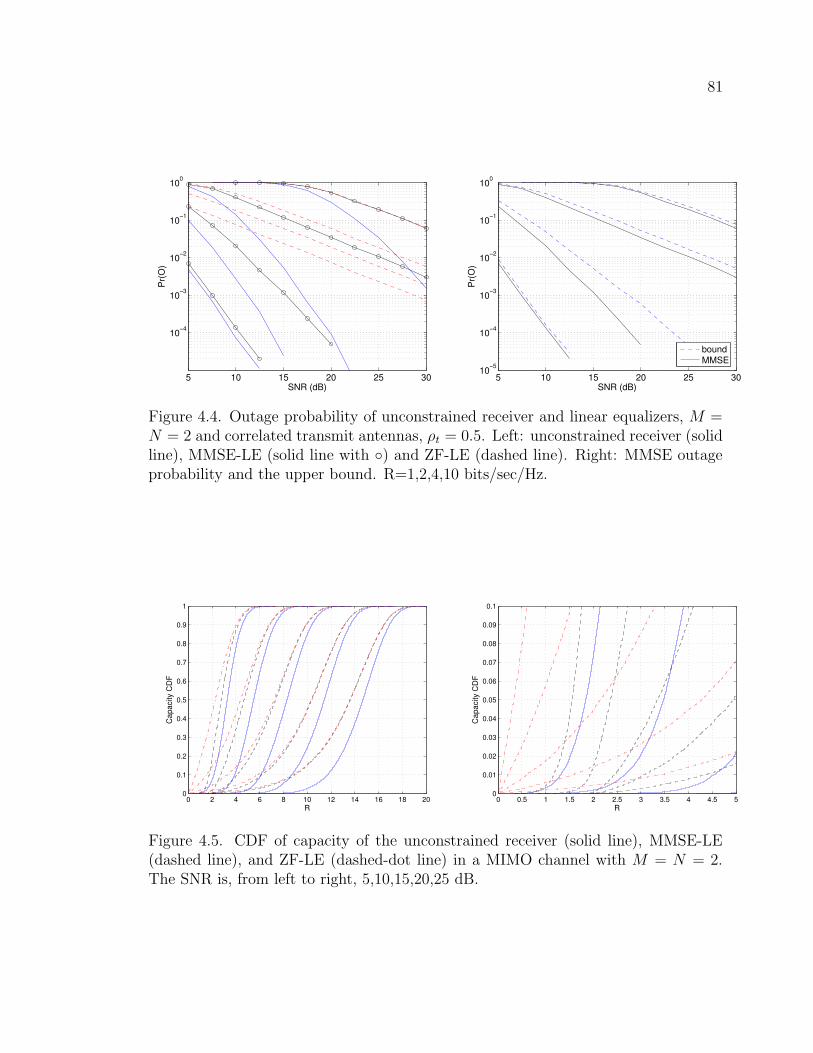
81
5 10 15 20 25 30
10−4
10−3
10−2
10−1
100
SNR (dB)
Pr(
O)
5 10 15 20 25 3010
−5
10−4
10−3
10−2
10−1
100
SNR (dB)
Pr(
O)
boundMMSE
Figure 4.4. Outage probability of unconstrained receiver and linear equalizers, M =N = 2 and correlated transmit antennas, ρt = 0.5. Left: unconstrained receiver (solidline), MMSE-LE (solid line with ) and ZF-LE (dashed line). Right: MMSE outageprobability and the upper bound. R=1,2,4,10 bits/sec/Hz.
0 2 4 6 8 10 12 14 16 18 200
0.1
0.2
0.3
0.4
0.5
0.6
0.7
0.8
0.9
1
R
Cap
acity
CD
F
0 0.5 1 1.5 2 2.5 3 3.5 4 4.5 50
0.01
0.02
0.03
0.04
0.05
0.06
0.07
0.08
0.09
0.1
R
Cap
acity
CD
F
Figure 4.5. CDF of capacity of the unconstrained receiver (solid line), MMSE-LE(dashed line), and ZF-LE (dashed-dot line) in a MIMO channel with M = N = 2.The SNR is, from left to right, 5,10,15,20,25 dB.
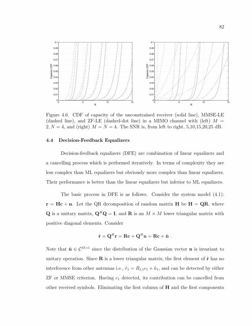
82
0 5 10 150
0.01
0.02
0.03
0.04
0.05
0.06
0.07
0.08
0.09
0.1
R
Cap
acity
CD
F
0 5 10 150
0.01
0.02
0.03
0.04
0.05
0.06
0.07
0.08
0.09
0.1
R
Cap
acity
CD
F
Figure 4.6. CDF of capacity of the unconstrained receiver (solid line), MMSE-LE(dashed line), and ZF-LE (dashed-dot line) in a MIMO channel with (left) M =2, N = 4, and (right) M = N = 4. The SNR is, from left to right, 5,10,15,20,25 dB.
4.4 Decision-Feedback Equalizers
Decision-feedback equalizers (DFE) are combination of linear equalizers and
a cancelling process which is performed iteratively. In terms of complexity they are
less complex than ML equalizers but obviously more complex than linear equalizers.
Their performance is better than the linear equalizers but inferior to ML equalizers.
The basic process in DFE is as follows. Consider the system model (4.1):
r = Hc + n. Let the QR decomposition of random matrix H be H = QR, where
Q is a unitary matrix, QHQ = I, and R is an M × M lower triangular matrix with
positive diagonal elements. Consider
r = QHr = Rc + QHn = Rc + n .
Note that n ∈ CM×1 since the distribution of the Gaussian vector n is invariant to
unitary operation. Since R is a lower triangular matrix, the first element of r has no
interference from other antennas i.e., r1 = R1,1c1 + n1, and can be detected by either
ZF or MMSE criterion. Having c1 detected, its contribution can be cancelled from
other received symbols. Eliminating the first column of H and the first components
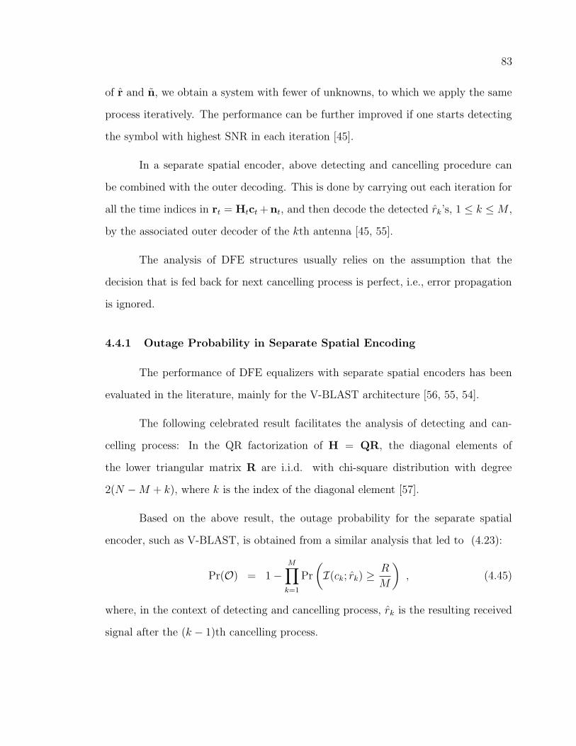
83
of r and n, we obtain a system with fewer of unknowns, to which we apply the same
process iteratively. The performance can be further improved if one starts detecting
the symbol with highest SNR in each iteration [45].
In a separate spatial encoder, above detecting and cancelling procedure can
be combined with the outer decoding. This is done by carrying out each iteration for
all the time indices in rt = Htct +nt, and then decode the detected rk’s, 1 ≤ k ≤ M ,
by the associated outer decoder of the kth antenna [45, 55].
The analysis of DFE structures usually relies on the assumption that the
decision that is fed back for next cancelling process is perfect, i.e., error propagation
is ignored.
4.4.1 Outage Probability in Separate Spatial Encoding
The performance of DFE equalizers with separate spatial encoders has been
evaluated in the literature, mainly for the V-BLAST architecture [56, 55, 54].
The following celebrated result facilitates the analysis of detecting and can-
celling process: In the QR factorization of H = QR, the diagonal elements of
the lower triangular matrix R are i.i.d. with chi-square distribution with degree
2(N − M + k), where k is the index of the diagonal element [57].
Based on the above result, the outage probability for the separate spatial
encoder, such as V-BLAST, is obtained from a similar analysis that led to (4.23):
Pr(O) = 1 −M∏
k=1
Pr
(
I(ck; rk) ≥R
M
)
, (4.45)
where, in the context of detecting and cancelling process, rk is the resulting received
signal after the (k − 1)th cancelling process.
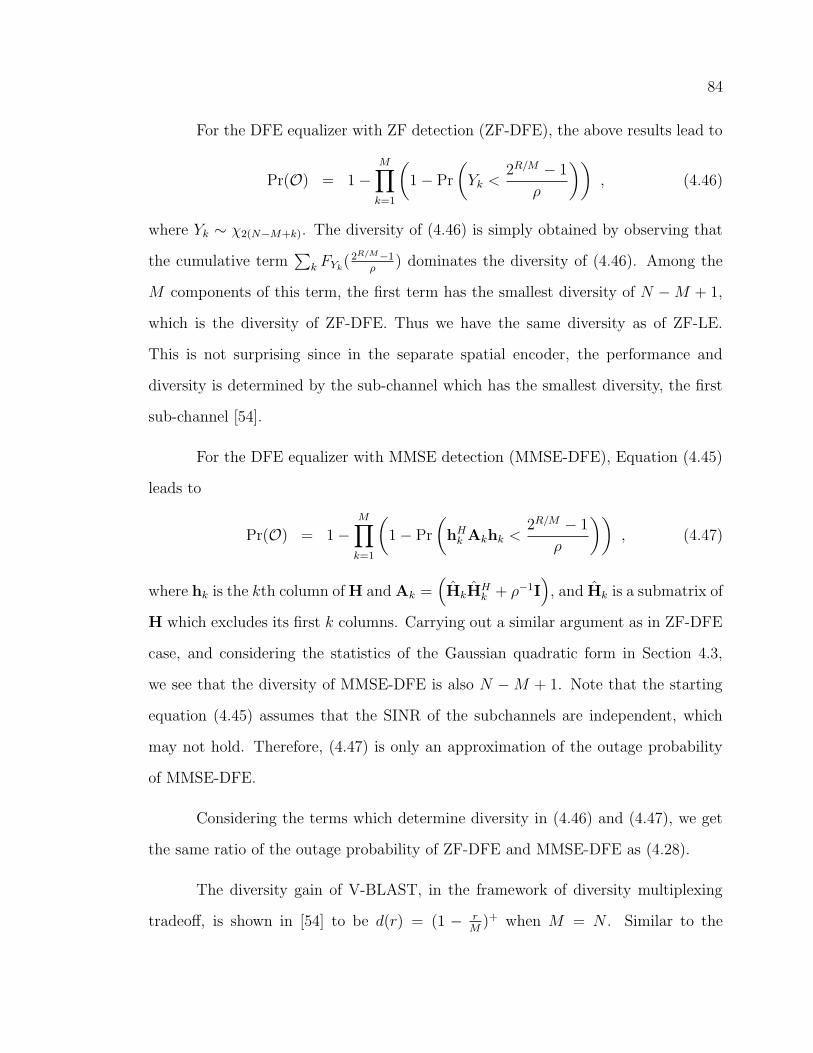
84
For the DFE equalizer with ZF detection (ZF-DFE), the above results lead to
Pr(O) = 1 −M∏
k=1
(
1 − Pr
(
Yk <2R/M − 1
ρ
))
, (4.46)
where Yk ∼ χ2(N−M+k). The diversity of (4.46) is simply obtained by observing that
the cumulative term∑
k FYk(2R/M−1
ρ) dominates the diversity of (4.46). Among the
M components of this term, the first term has the smallest diversity of N − M + 1,
which is the diversity of ZF-DFE. Thus we have the same diversity as of ZF-LE.
This is not surprising since in the separate spatial encoder, the performance and
diversity is determined by the sub-channel which has the smallest diversity, the first
sub-channel [54].
For the DFE equalizer with MMSE detection (MMSE-DFE), Equation (4.45)
leads to
Pr(O) = 1 −M∏
k=1
(
1 − Pr
(
hHk Akhk <
2R/M − 1
ρ
))
, (4.47)
where hk is the kth column of H and Ak =(
HkHHk + ρ−1I
)
, and Hk is a submatrix of
H which excludes its first k columns. Carrying out a similar argument as in ZF-DFE
case, and considering the statistics of the Gaussian quadratic form in Section 4.3,
we see that the diversity of MMSE-DFE is also N − M + 1. Note that the starting
equation (4.45) assumes that the SINR of the subchannels are independent, which
may not hold. Therefore, (4.47) is only an approximation of the outage probability
of MMSE-DFE.
Considering the terms which determine diversity in (4.46) and (4.47), we get
the same ratio of the outage probability of ZF-DFE and MMSE-DFE as (4.28).
The diversity gain of V-BLAST, in the framework of diversity multiplexing
tradeoff, is shown in [54] to be d(r) = (1 − rM
)+ when M = N . Similar to the
85
procedure in Section 4.3.1, above result can be extended to the case where N ≥ M
which gives d(r) = (L + 1)(1 − rM
)+.
4.4.2 Outage Probability in Joint Spatial Encoding
The outage probability for the joint encoding structure has been investigated
in the literature. Particularly, the D-BLAST architecture has been analyzed in the
early work of [46] and recently in [54].
In the joint spatial encoding architecture, outage occurs when the sum of
mutual information of the sub-channels is less than the target rate. The sum mutual
information is given by (4.31), except that rk is the result of the (k − 1)th cancelling
process.
When the ZF-DFE equalizer is applied to D-BLAST, [54] has shown that the
diversity is N(N + 1)/2, assuming M = N .
With perfect decision-feedback, the MMSE-DFE equalizer is actually capacity-
achieving (see e.g. [38]), hence it achieves the full diversity of the unconstrained
decoder. In the general context of joint spatial encoding, [38] shows that the sum
mutual information in (4.31) is the capacity of the MIMO system. In the context of
diversity multiplexing tradeoff, [54] shows that MMSE-DFE receiver for D-BLAST
structure achieves the tradeoff of the underlying MIMO channel.
4.5 Simulation Results
We consider a MIMO system with M = N = 2. The outage probability of
DFE equalizers in separate spatial encoding is shown in Figure 4.7. Both ZF-DFE
and MMSE-DFE equalizers show the diversity M−N +1 = 1, the same as their linear
counterparts, but they have better performance compared to linear equalizers. We
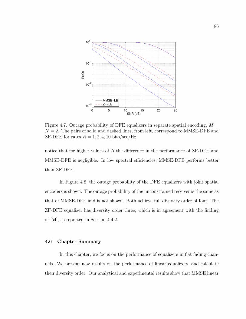
86
0 5 10 15 20 2510
−3
10−2
10−1
100
SNR (dB)
Pr(
O)
MMSE−LEZF−LE
Figure 4.7. Outage probability of DFE equalizers in separate spatial encoding, M =N = 2. The pairs of solid and dashed lines, from left, correspond to MMSE-DFE andZF-DFE for rates R = 1, 2, 4, 10 bits/sec/Hz.
notice that for higher values of R the difference in the performance of ZF-DFE and
MMSE-DFE is negligible. In low spectral efficiencies, MMSE-DFE performs better
than ZF-DFE.
In Figure 4.8, the outage probability of the DFE equalizers with joint spatial
encoders is shown. The outage probability of the unconstrained receiver is the same as
that of MMSE-DFE and is not shown. Both achieve full diversity order of four. The
ZF-DFE equalizer has diversity order three, which is in agreement with the finding
of [54], as reported in Section 4.4.2.
4.6 Chapter Summary
In this chapter, we focus on the performance of equalizers in flat fading chan-
nels. We present new results on the performance of linear equalizers, and calculate
their diversity order. Our analytical and experimental results show that MMSE linear
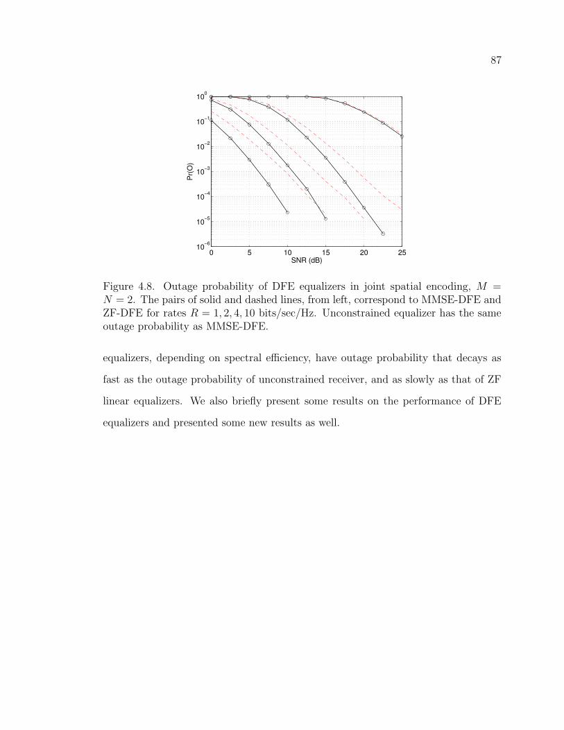
87
0 5 10 15 20 2510
−6
10−5
10−4
10−3
10−2
10−1
100
SNR (dB)
Pr(
O)
Figure 4.8. Outage probability of DFE equalizers in joint spatial encoding, M =N = 2. The pairs of solid and dashed lines, from left, correspond to MMSE-DFE andZF-DFE for rates R = 1, 2, 4, 10 bits/sec/Hz. Unconstrained equalizer has the sameoutage probability as MMSE-DFE.
equalizers, depending on spectral efficiency, have outage probability that decays as
fast as the outage probability of unconstrained receiver, and as slowly as that of ZF
linear equalizers. We also briefly present some results on the performance of DFE
equalizers and presented some new results as well.
CHAPTER 5
PERFORMANCE OF EQUALIZERS IN FREQUENCY-SELECTIVE
MULTIPLE-ANTENNA FADING CHANNELS
In frequency-selective MIMO channels interference occurs across both time and
space. In this section, we analyze the performance of various equalizers in frequency-
selective MIMO channels. Prior work in this area were focused mainly on diversity
combining [44, 58, 59]. The performance of ML receiver is evaluated first in spatially
uncorrelated and correlated channels. We also provide results for channels whose
multipath fading components are correlated. Next, we analyze the performance of
linear equalizers and calculate their achievable diversity order.
5.1 Introduction
Assume a MIMO channel with M transmit antennas, N receive antennas,
and memory ν. Such a channel is represented by matrix channels H0,H1, · · · ,Hν ∈
CN×M , with the system model r = Hc + n, i.e.
rL
rL−1...r1
=
H0 H1 · · · Hν 0 · · · 00 H0 H1 · · · Hν · · · 0...
. . . . . . . . . . . . . . ....
0 · · · 0 H0 H1 · · · Hν
cL
cL−1...c1
+
nL
nL−1...n1
, (5.1)
where L is the block length, ct is the M × 1 transmit vector at time index t, rt is the
N×1 received vector at the same time index, nt ∈ CN×1 is AWGN, and H ∈ CLN×LM
is the equivalent channel.
88
89
5.2 Maximum Likelihood Equalizer
In this section, we use methodology and notation similar to Section 3.2. Let
H = (Hν ,Hν−1, · · · ,H0), where H ∈ CN×(ν+1)M , and denote the jth row of H with
hj. The ML metric in this case is
||H∆||2 = ∆HH
HH∆
where ∆ =(
∆H1 ,∆H
2 , · · · ,∆HL
)H, and ∆t = ct − ct, where ct and ct are the tth
subvector of the codewords c and c. The structure of the matrix H simplifies the ML
metric to
||H∆||2 =L−ν∑
i=0
AHi HHHAi (5.2)
=L−ν∑
i=0
N∑
j=1
AHi hH
j hjAi =N∑
j=1
hjΩhHj , (5.3)
where Ai4=(
∆Hi , · · · ,∆H
ν+i
)Hand Ω =
∑L−νi=0 AiA
Hi . The ML metric is a sum of
quadratic forms. Using the result of [32], appeared as a Lemma in Section 3.2, we
obtain the following MGF for Γ = ||H∆||2, assuming the channel components Hi are
independent:
ΦΓ(s) =νM∏
i=0
(1 − sλi)−N , (5.4)
where s4= − ρ
4 sin2 θ, ρ = Ex
N0, and λi is an eigenvalue of Ω. Asymptotically, ΦΓ(s)
behaves like
ΦΓ(−s)·=∏
λi 6=0
(sλi)−N =
s−NM(ν+1)
det(Ω)N,
where for the second equality it is assumed that all the eigenvalues λi are nonzero.
If Ω is full rank, ΦΓ(s) decays with the (ν + 1)MN power of SNR, indicating the
maximum obtainable diversity. However, to achieve this diversity, coding is necessary,
as demonstrated below.
90
If the vector c does not have any redundancy, then c and c are different in at
most one position, hence only one ∆t is non-zero. Assume that the position of the
nonzero ∆t is far enough from the edges of ∆ such that exactly ν+1 of Ai vectors are
nonzero. Therefore, Ω = I⊗D, where D is an M ×M matrix which has exactly one
nonzero diagonal element. Hence Ω has rank ν + 1, i.e., diversity order (ν + 1)N . It
follows that frequency and receive diversity are possible without coding, but transmit
diversity requires coding, or otherwise a carefully designed signaling that guarantees
a full rank Ω.
We now calculate the MGF of Γ when the channel matrices Hi are not in-
dependent. Assume Hν(i, j), · · · ,H0(i, j) are correlated with correlation matrix Rt,
which is fixed for all pairs of i and j. This model assumes that all antenna pairs
in the MIMO system have the same temporal dynamics. The covariance of hj,the
jth row of H, is Rt ⊗ IM . The vector hj can be decorrelated by the transform
hj = hj (Rt ⊗ IM)1
2 where hj is a white vector. Hence
||H∆||2 =N∑
j=1
hj (Rt ⊗ IM)1
2 Ω (Rt ⊗ IM)H2 hH
j ,
which results in the following MGF
ΦΓ(s) =νM∏
i=0
(I − sµi)−N , (5.5)
where µi are eigenvalues of (Rt ⊗ IM)Ω. We notice that as long as the covariance
matrix Rt is full-rank, the diversity obtained by ML equalizer is not affected by
channel correlation, but it incurs performance loss characterized by (det(Rt))M .
We now consider the spatial correlation between the elements of Hi. We again
use the channel model (4.7). In case of transmit-side correlation only (RRx = IN and
RRx 6= IM), we obtain the following MGF:
ΦΓ(s) =νM∏
i=0
(I − sµi)−N ,
91
where µi are eigenvalues of (Rt ⊗RRx)Ω. If RRx 6= IN and RRx 6= IM , the procedure
we have the following expression for MGF:
ΦΓ(s) = det (I − s(Rt ⊗ RRx)(RRx ⊗ Ω))−1 .
We notice that in the correlated channel cases, asymptotic behavior of MGF is inde-
pendent of correlation as long as the correlation matrices are full-rank, and the loss
in performance is quantified with the determinant of the correlation matrices, similar
to (3.14).
5.3 Linear Equalizers
We consider block transmission and apply linear equalization in matrix-form.
A linear transformation is applied to the received signal in a single step to remove
both temporal and spatial interference (see [38], among others).
Assume the system model (5.1). The block ZF-LE has the matrix form:
FZF = (HHH)−1
HH , (5.6)
which transforms the received signal to
r = FZF r = c + (HHH)−1
HHn . (5.7)
The MMSE-LE is
FMMSE = (HHH + ρ−1I)−1
HH , (5.8)
which transforms the received signal to
r = FMMSE r = (HHH + ρ−1I)−1
HH
Hc + (HHH + ρ−1I)−1
HHn . (5.9)
For mathematical tractability, we assume that the data sent from each transmit
antenna is appended by a cyclic prefix (CP). The CP converts the channel matrix
92
H to a block circulant matrix. A block circulant matrix with size LN × LM is a
matrix whose sub-matrices, each with size N × M , appear in a circulant fashion.
Block diagonalization of block circulant matrices is possible using the following fact.
Fact: Let H be a block circulant matrix of size LN × LM . Then H = (Q ⊗
IN)Λ(QH ⊗ IM), where Q is the Discrete Fourier Transform (DFT) matrix as defined
in Section 3.3, and Λ is a block diagonal matrix whose diagonal matrices are
Λ` =1√L
ν+1∑
k=1
Hk e−(k−1)(`−1)/L ,
for ` = 1, · · · , L, and ν + 1 ≤ L.
Assuming Hi ∈ CN×M , i = 1, · · · , ν + 1 are independent, then Λ` ∈ CN×M
for ` = 1, · · · , L, since Λ`(i, j) is a weighted sum of Hk(i, j). However, Λ`’s are not
necessarily independent. If L = ν +1, which the circulant channel matrix H becomes
fully populated, Λ`’s are independent. Our analysis is limited to this case, but our
experimental results confirm that the findings of the uncorrelated case is also valid
for L 6= ν + 1.
5.3.1 ZF-LE
In the case of ZF-LE, the equivalent noise is n4= (HH
H)−1HHn, with covari-
ance matrix Rn = σ2n(HH
H)−1. Using the block circulant channel model, the noise
covariance is
Rn = σ2n(Q ⊗ IM)
(
ΛHΛ)−1
(QH ⊗ IM) . (5.10)
The properties of the orthogonal matrix Q result in a block diagonal structure for
Rn whose blocks, denoted by B, are all the same
B =1
L
L∑
`=1
(
ΛH` Λ`
)−1. (5.11)
93
Each ΛH` Λ` is a Wishart matrix, hence B is a sum of independent inverse Wishart
matrices whose diagonal elements determine the decision-point SINR. In Section 4.3,
we show that the diagonal elements of an inverse Wishart matrix are independent.
The decision-point SINR of each symbol, denoted by γi for i = 1, · · · ,M , is
γi =ρ
1L
L∑
`=1
Y`,i
, (5.12)
where Y`,i, ` = 1, · · · , L, is the ith diagonal elements of(
ΛH` Λ`
)−1and X`,i
4= 1
Y`,i∼
χ2(N−M+1). Since the diagonal blocks of Rn are equal, we have γ(jM+i) = γi for
j = 0, · · · , L − 1. Equation (5.12) is a generalization of the decision-point SINR in
frequency-selective SISO channel given by (3.24). Since the CDF of γi’s are the same,
the subscript i is dropped in the following unless needed for clarity.
FΓ(γ) = Pr(Γ < γ)
= Pr
(
L∑
`=1
1
X`
>ρL
γ
)
. (5.13)
We evaluate (5.13) for γ → 0+ based on the similarity between the integration region
of (5.13) and what we carry out in Section 3.3.
When γ → 0+ the integration region of (5.13) is approximated by L regions
where the `th region is defined as 0 ≤ X` ≤ γρL
, and for k 6= `, 0 ≤ Xk. Recalling
that X` ∼ χ2(N−M+1), and denoting α4= γ
ρL, (5.13) gives
FΓ(γ) = L
∫ α
0
fX1(x1)dX1
L∏
`=2
∫ ∞
0
fX`(x`)dX`
= LFX1(α) = L
(
1 − e−α
N−M+1∑
i=1
αi−1
(i − 1)!
)
·=
1
(N − M + 1)!LN−M
(
γ
ρ
)N−M+1
, (5.14)
where the multiple count of the intersection of the regions is ignored because it de-
creases as fast as γL(N−M+1) when γ → 0+, hence does not change the result of (5.14).
94
The achievable diversity is N −M +1, which is the same diversity order as what ZF-
LE achieves in flat fading channel (see Section 4.3). Therefore, ZF-LE is incapable of
achieving the frequency diversity.
Outage Probability
We analyze the outage probability of ZF-LE in frequency-selective channel
for separate and joint spatial encoders. In separate spatial coding, the CDF of the
SNR of the individual symbols determine the outage probability, seen from (4.23)
and (4.24). From (5.14), we conclude that the outage probability of ZF-LE decreases
as ρ−(N−M+1).
In the joint spatial encoding architecture, Equation (4.31) can be rewritten as
follows
Pr(O) = Pr
(
1
L
LM∑
k=1
log(1 + γk) < R
)
= Pr
(
M∑
k=1
log(1 + γk) < R
)
(5.15)
≈ Pr
(
M∑
k=1
log(γk) < R
)
(5.16)
where γk is given by (5.12), Equation (5.15) is due to γ(jM+i) = γi, j = 0, · · · , L − 1,
and the approximation in (5.16) is made for tractability. Applying Jensen’s inequality,
and substituting (5.12) in, we obtain the following upper bound
Pr(O) ≤ Pr
(
M∑
k=1
L∑
`=1
1
X`,k
> ρL2−R
)
. (5.17)
The earlier result of independence of XjM , · · · , XjM+i, for a given j where j =
0, · · · , L − 1, and the assumption of L = ν + 1 make all Xk’s independent with
chi-square distribution with 2(N − M + 1) degrees of freedom. Calculated in the
95
same manner as (5.13), in high-SNR region (5.17) is
Pr(O) ≤ M2R(N−M+1)
(N − M + 1)!LN−Mρ−(N−M+1) . (5.18)
5.3.2 MMSE-LE
The decision-point SINR of the received symbols after MMSE linear equaliza-
tion are equal to [38]
γi =1
(
ρHH
H + I)−1
i
− 1 , (5.19)
for i = 1, · · · , LM , where M−1i is the ith diagonal element of the inverse of the matrix
M. Using ILM = (Q ⊗ IM)(QH ⊗ IM) and
ρHH
H + ILM = (Q ⊗ IM)(
ρΛHΛ + ILM
)
(QH ⊗ IM) ,
the SINR in (5.19), for i = 1, · · · ,M , can be simplified to
γi =1
1L
L∑
`=1
(IM + ρΛH` Λ`)
−1
i
− 1 . (5.20)
Statistical evaluation of (5.20) appears to be difficult. To obtain the performance and
diversity order of MMSE-LE, we resort to outage analysis.
Outage Probability
In joint spatial encoding architecture, starting from (5.15), the outage proba-
bility is:
Pr(O) = Pr
(
M∑
k=1
log(1 + γk) < R
)
= Pr
(
M∑
k=1
log
(
1
L
L∑
`=1
(
IM + ρΛH` Λ`
)−1
k
)
> −R
)
, (5.21)
96
where the involvement of the diagonal elements makes the evaluation of the outage
probability intractable. However, an upper bound to above outage probability can be
calculated as follows. Denote A`4= 1
L(IM + ρΛH
` Λ`)−1. Applying Jensen’s inequality
to the argument of (5.21) gives
M∑
k=1
log
(
L∑
`=1
(A`)k
)
≤ M log
(
1
M
L∑
`=1
tr (A`)
)
= M log
(
1
LM
L∑
`=1
M∑
k=1
1
1 + ρλ`,k
)
, (5.22)
where λ`,i are eigenvalues of ΛH` Λ`. Application of (5.22) in (5.21) gives the following
upper bound :
Pr(O) ≤ Pr
(
L∑
`=1
M∑
k=1
1
1 + ρλ`,k
≥ LM2−R
LM
)
. (5.23)
For SISO channel, above bound becomes exact and the same as (3.38). In flat fading
channel (L = 1), the above upper bound becomes the same (4.39). We evaluate (5.23)
for high and low spectral efficiencies.
For small values of R, the outage region of (5.23) is a polyhedron in the space
of eigenvalues λ`,k whose vertices are the points on the axes with value
cν,M4=
1 + M − Lb
ρM(Lb − 1)
where b = 2−RM . This region is the bounded region in the positive cone separated by
the planeL∑
`=1
M∑
k=1
λ`,k = cν,M . The upper bound (5.23) can be evaluated by plugging
in the distribution of the eigenvalues λ`,k and integrating over the polyhedron outage
region. For M = N = 2 and a two-tap channel, the upper bound for small values of
97
R is
Pr(O) ≤ Pr
(
1
1 + ρλ1,1
+1
1 + ρλ1,2
+1
1 + ρλ2,1
+1
1 + ρλ2,2
≥ 22−R2
)
=
∫ ∫
A1
(λ1,1 − λ1,2)2 e−λ1,1−λ1,2
×∫ ∫
A2
(λ2,1 − λ2,2)2 e−λ2,1−λ2,2dλ1,1dλ1,2dλ2,1dλ2,2
·=
4
45c81,2 =
4c81,2
45ρ−8 , (5.24)
where A1 ≡ λ1,1 + λ1,2 ≤ c1,2 and A2 ≡ λ2,1 + λ2,2 ≤ c1,2 − λ1,1 − λ1,2, and
c1,2 = 3−21−R/2
21−R/2−1. The above upper bound decays as fast as ρ−8, indicating the diversity
order of eight. For other values of M , N , and ν, the upper bound (5.23) can be
calculated to obtain the diversity order of MN(ν + 1) in low spectral efficiency.
For large values of R, the outage region of (5.23) is approximated by LM
regions. The (`, k)th region, ` = 1, · · · , L and k = 1, · · · ,M , is defined as 0 ≤ λ`,k ≤
bν,M , and for (ˆ, k) 6= (`, k), λ ˆ,k ≥ 0, where bν,M = 1ρ
(
2RM
LM− 1
)
. The evaluation
of (5.23) is similar to (4.44) and results in an expression which decays as fast as
ρN−M+1. Therefore, the diversity order in high spectral efficiencies is N − M + 1.
5.3.3 Simulation Results
Consider a MIMO system with two antennas in the transmit and receive sides
(M = N = 2) in a two-tap Rayleigh frequency-selective channel (ν = 1) and block
length L = 10. The outage probability of the linear equalizers in joint spatial ar-
chitecture are shown in Figure 5.1. The target rate is R = 2, 4, 6, 8 bits/sec/Hz. As
expected, ZF-LE shows diversity order of N−M +1 = 1, regardless of the target rate.
This confirms that ZF-LE cannot harvest the frequency diversity of the channel.
However, MMSE-LE behaves differently in various spectral efficiencies. For
small values of R, the diversity order is very close to that of the unconstrained receiver.
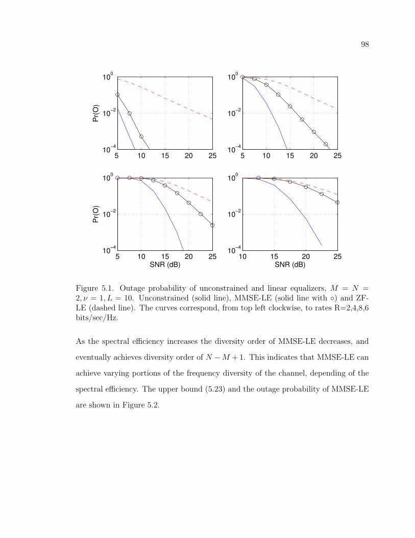
98
5 10 15 20 2510−4
10−2
100
Pr(
O)
5 10 15 20 2510−4
10−2
100
5 10 15 20 2510−4
10−2
100
Pr(
O)
SNR (dB)10 15 20 25
10−4
10−2
100
SNR (dB)
Figure 5.1. Outage probability of unconstrained and linear equalizers, M = N =2, ν = 1, L = 10. Unconstrained (solid line), MMSE-LE (solid line with ) and ZF-LE (dashed line). The curves correspond, from top left clockwise, to rates R=2,4,8,6bits/sec/Hz.
As the spectral efficiency increases the diversity order of MMSE-LE decreases, and
eventually achieves diversity order of N −M + 1. This indicates that MMSE-LE can
achieve varying portions of the frequency diversity of the channel, depending of the
spectral efficiency. The upper bound (5.23) and the outage probability of MMSE-LE
are shown in Figure 5.2.
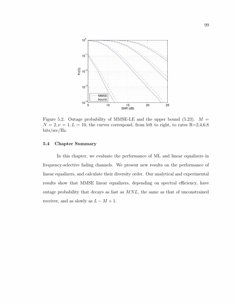
99
5 10 15 20 2510
−4
10−3
10−2
10−1
100
Pr(
O)
SNR (dB)
MMSEbound
Figure 5.2. Outage probability of MMSE-LE and the upper bound (5.23). M =N = 2, ν = 1, L = 10, the curves correspond, from left to right, to rates R=2,4,6,8bits/sec/Hz.
5.4 Chapter Summary
In this chapter, we evaluate the performance of ML and linear equalizers in
frequency-selective fading channels. We present new results on the performance of
linear equalizers, and calculate their diversity order. Our analytical and experimental
results show that MMSE linear equalizers, depending on spectral efficiency, have
outage probability that decays as fast as MNL, the same as that of unconstrained
receiver, and as slowly as L − M + 1.
CHAPTER 6
CONCLUSIONS AND FUTURE WORK
6.1 Contributions
In Chapter 2, we analyze the role of redundancy in a concatenated entropy
and channel code. The significance of such concatenated codes is indisputable because
entropy coding is part of any compression system, and channel codes are always used
for reliable transmission.
Previous work in the area of joint entropy and channel coding were limited in
either decoding or the amount of redundancy in the entropy code. In some of the
early works, the redundancy of the entropy codes was exploited by simple but sub-
optimal decoding, such as bi-directional decoding in RVLC, which has the limitation
of separate source channel decoding. In some recent works [1, 9], joint source channel
decoding was used via iterative decoding methods. However, no attention was given
to the amount of redundancy in entropy codes.
We extend the prior work in joint entropy and channel coding as follows. We
generalize the role of entropy codes by using variable-length error correcting codes
of [4, 5]. Subject to a total rate, we allow the outer entropy code and inner channel
code freely share the available rate. We analyze the error rate of the concatenated code
to obtain design rules for the constituent codes. We consider iterative decoding and
improve upon it by using list iterative decoding. Our results indicate that allowing
more redundancy in entropy codes improves the overall code significantly compared
to the concatenated RVLC and channel code.
100
101
We also compare the proposed concatenated code with a code that consists
of Huffman entropy code and a serial concatenated channel code. We conclude that
there is no clear and universal advantage of any of the two codes.
In Chapters 3, 4, and 5 we analyze the performance of equalizers in fading
channels which experience interference in time or space or both. Our analysis relies
on either the statistical evaluation of the decision-point SNR, or outage probability.
In Chapter 3, we consider a frequency selective single-antenna fading channel
and analyze the performance of various linear and decision-feedback equalizers. We
determine the diversity order of linear equalizers and show that ZF-LE does not
achieve any of the available frequency diversity. However, MMSE-LE may achieve
the full diversity if the spectral efficiency is low, or none if the spectral efficiency is
high. In intermediate spectral efficiencies, MMSE-LE achieves some diversity which
is less than the full diversity order.
We consider a flat fading multiple-antenna in Chapter 4, and analyze the
performance of various equalizers for two spatial encoding architectures. The diversity
order of ZF-LE has been shown by [51] to be N −M +1. Traditionally, it is expected
that MMSE-LE performs the same as ZF-LE in high SNR regime. However, our
findings show that it can perform quite differently than ZF-LE. In separate spatial
encoding, both linear equalizers have the diversity order N−M +1, however, MMSE-
LE performs better in low spectral efficiencies regardless on SNR. In joint spectral
efficiency, ZF-LE achieves the same diversity order N − M + 1. In low spectral
efficiency, MMSE-LE achieves the full spatial diversity of the system. As the spectral
efficiency grows, the diversity order of MMSE-LE decreases and eventually becomes
the same as ZF-LE. In Chapter 4, we also present some new results on the performance
of decision-feedback equalizers. In separate spatial encoding, ZF-DFE and MMSE-
102
DFE do not achieve any higher diversity order than the linear equalizers, although
they have better performance.
In Chapter 5, frequency-selective multiple-antenna fading channels are consid-
ered where the interference occurs in both space and time. We analyze the perfor-
mance of ML equalizers in uncorrelated and correlated channels. Though the perfor-
mance of ML equalizers degrade in correlated channels, the diversity order remains
unchanged. We also analyzed the performance of linear equalizers. Our findings show
that ZF-LE achieve the diversity order of N − M + 1 which is the same as what it
achieves in flat fading channel. Therefore, similar to the results of Chapter 3, ZF-
LE is incapable of harvesting the available frequency diversity. However, MMSE-LE
achieves the full spatial and frequency diversity of MN(ν + 1) if it operates in low
spectral efficiency. As the spectral efficiency grows, the diversity order of MMSE-LE
decreases and finally becomes the same as that of ZF-LE.
6.2 Future Work
Related to the material in Chapter 2, the issue of rate allocation in concate-
nated codes is an open problem. Given a fixed total rate, there is a tradeoff in what
share of the rate the outer and inner codes of a serially concatenated code should
have. The higher amount of redundancy given to the outer code, the larger interleav-
ing gain. However, less amount of redundancy becomes available to the inner code
and the overall performance may not be optimum especially in low to moderate SNR.
The issue of rate allocation to constituent codes of a concatenated code is of
value in many scenarios. In the framework of Chapter 2, it is of interest to know how
much the outer VLC code should be redundant to have the best performance. For
example, in Section 2.7, we notice that the concatenated code with higher dof does
103
not perform better than a code with a more balanced rate allocation. Similarly, se-
rially concatenated convolutional codes that allocate the overall rate efficiently have
better performance. The optimal rate allocation is of importance in other concate-
nated codes [60], such as hybrid concatenated codes and double serially concatenated
codes [61].
In Chapters 3, 4, and 5, we evaluate the performance of various equalizers in
a single-user environment where the interference occurs between the components of
each user’s signal in time or space or both. In multiuser environments, the interference
may also occur between the users’ signals if they do not communicate in orthogonal
channels. While the performance of equalizers has been investigated in multiuser
environments [51, 62, 63], a comprehensive analysis of linear and decision-feedback
equalizers has not been presented yet. The performance of ZF-LE in a multiple-
access flat fading channel with receive diversity is investigated in [51]. In [62], it is
shown that MMSE-DFE achieves the capacity of a multiple-access Gaussian channel.
The focus of [51, 62] is limited to frequency-nonselective channels. Tse, Viswanath
and Zheng [63] presented the most comprehensive analysis recently by considering a
multiple-access channel where the users and the receiver have multiple antennas.
However, there are many open problems when the channel is frequency-selective.
The performance of equalizers in a frequency-selective multi-user environment has not
been yet investigated analytically. In such a scenario, when the receiver has multiple
antennas, multiuser interference can be removed more easily. When users are also
equipped with multiple antennas, although the available diversity of the channel in-
creases, the spatial interference of each user’s data must be dealt with along with
temporal and multiuser interference.
Performance of frequency-selective channels can also be investigated in the
framework of diversity-multiplexing tradeoff [54, 63]. Recently, the diversity-multiplexing
104
tradeoff of frequency-selective channels in a single-antenna single-user environment
has been investigated [64]. The optimal tradeoff of frequency-selective multiple-access
channels has not been reported yet and is considered an open problem. It is also of
interest to see how linear and decision-feedback equalizers perform, compared to the
optimal tradeoff of the channel, and what portion of the maximum diversity they can
achieve.
BIBLIOGRAPHY
[1] R. Bauer and J. Hagenauer, “On variable length codes for iterative source/channel
decoding,” in Proc. Data Compression Conference, April 2001, pp. 273–282.
[2] S. Benedetto, D. Divsalar, G. Montorsi, and F. Pollara, “Serial concatenation of
interleaved codes: performance analysis, design, and iterative decoding,” IEEE
Transactions on Information Theory, vol. 44, no. 3, pp. 909 –926, May 1998.
[3] Y. Takishima, M. Wada, and H. Murakami, “Reversible variable length codes,”
IEEE Transactions on Communications, vol. 43, pp. 158–162, February/March/April
1995.
[4] V. Buttigieg, “Variable-Length Error-Correcting Codes,” Ph.D. Thesis, Depart-
ment of Electrical Engineering, University of Manchester, 1995.
[5] V. Buttigieg and P. G. Farrell, “Variable-length error-correcting codes,” IEE
Proceedings-Communications, vol. 147, no. 4, pp. 211–215, August 2000.
[6] K. P. Subbalakshmi and J. Vaisey, “On the joint source-channel decoding of
variable-length encoded sources: The BSC case,” IEEE Transactions on Com-
munications, vol. 49, pp. 2052–2055, December 2001.
[7] K. P. Subbalakshmi and J. Vaisey, “Joint source-channel decoding of entropy
coded markov sources over binary symmetric channels,” in Proc. IEEE ICC,
1999, pp. 446–450.
105
106
[8] C. Berrou and A. Glavieux, “Near optimum error correcting coding and decod-
ing: Turbo codes,” IEEE Transactions on Communications, vol. 44, pp. 1261
–1271, October 1996.
[9] R. Bauer and J. Hagenauer, “Iterative source/channel decoding using reversible
variable-length codes,” in Proc. Data Compression Conference, April 2000, pp.
93–102.
[10] N. Goertz, “On the iterative approximation of optmal joint source-channel de-
coding,” Journal on Selected Areas in Communications, September 2001.
[11] A. Guyader, E. Fabre, C. Guillemot, and M. Robert, “Joint source-channel turbo
decoding of entropy-coded sources,” Journal on Selected Areas in Communica-
tions, vol. 9, pp. 1680–1696, September 2001.
[12] K. Lakovic and J. Villasenor, “Combining variable-length codes and turbo
codes,” in Proc. IEEE Vehicular Technology Conference, Spring 2002, pp. 1719
–1723.
[13] A. Hedayat and A. Nosratinia, “List-decoding of variable-length codes with
application in joint source-channel coding,” in Proc. Asilomar Conference on
Signals, Systems and Computers, 2002.
[14] A. Hedayat and A. Nosratinia, “On joint iterative decoding of variable-length
source codes and channel codes,” in Proc. of 40th Annual Allerton Conference
on Communication, Control, and Computing, 2002.
[15] A. Hedayat and A. Nosratinia, “Concatenated error-correcting entropy codes
and channel codes,” in Proc. IEEE ICC, May 2003, vol. 5, pp. 3090–3094.
107
[16] A. Hedayat and A. Nosratinia, “Performance analysis and design criteria for
finite-alphabet source/channel codes,” IEEE Transaction on Communications,
to appear, November 2004.
[17] A. Hedayat and A. Nosratinia, “Iterative and list decoding of concatenated
source/channel codes,” Eurasip Journal of Applied Signal Processing, Special
issue on Turbo Processing, to appear, November 2004.
[18] T. Okuda, E. Tanaka, and T. Kasai, “A method for correction of grabled words
based on the Levenshtein metric,” IEEE Transactions on Computers, vol. C-25,
pp. 172–176, February 1976.
[19] V. B. Balakirsky, “Joint source-channel coding with variable length codes,” in
Proc. IEEE ISIT, June 1997, p. 419.
[20] A. Murad and T. Fuja, “Robust transmission of variable-length encoded sources,”
in Proc. IEEE Wireless Communications and Networking Conference, Septem-
ber 1999.
[21] D. Divsalar and R. J. McEliece, “On the design of generalized coding systems
with interleavers,” JPL Progress Report, August 1998.
[22] J. Hagenauer, E. Offer, and L. Papke, “Iterative decoding of binary block and
convolutional codes,” IEEE Transactions on Information Theory, vol. 42, pp.
429–445, March 1996.
[23] S. Benedetto, D. Divsalar, G. Montorsi, and F. Pollara, “A soft-input soft-output
APP module for iterative decoding of concatenated codes,” IEEE Communica-
tions Letters, vol. 1, no. 1, pp. 22–24, January 1997.
108
[24] L. R. Bahl, J. Cocke, F. Jelinek, and J. Raviv, “Optimal decoding of linear codes
for minimizing symbol error rate,” IEEE Transactions on Information Theory,
vol. 20, pp. 284–287, March 1974.
[25] D. Divsalar, S. Dolinar, and F. Pollara, “Iterative turbo decoder analysis based
on density evolution,” Journal on Selected Areas in Communications, vol. 19,
pp. 891–907, May 2001.
[26] S. ten Brink, “Convergence behavior of iteratively decoded parallel concate-
nated codes,” IEEE Transactions on Communications, vol. 49, pp. 1727–1737,
October 2001.
[27] N. Seshadri and C.-E. W. Sundberg, “List Viterbi decdoing algorithms with
applications,” IEEE Transactions on Communications, vol. 43, pp. 313–323,
February/March/April 1994.
[28] K. R. Narayanan and G. L. Stuber, “List decoding of turbo codes,” IEEE
Transactions on Communications, vol. 46, pp. 754–762, June 1998.
[29] S. B. Wicker, Error Control Systems for Digital Communcation and Storage,
Englewood Cliffs, NJ: Prentice Hall, 1995.
[30] A. Hedayat, A. Nosratinia, and N. Al-Dhahir, “On the diversity order of linear
equalizers in fading channels,” in Proc. Asilomar Conference on Signals, Systems
and Computers, 2004.
[31] M. K. Simon and M.-S. Alouini, Digital Communication over Fading Channels:
A Unified Approach to Performance Analysis, John Wiley and Sons, New York,
2000.
109
[32] G. L. Turin, “The characteristic function of Hermetian quadratic forms in com-
plex normal random variables,” Biometrika, pp. 199–201, June 1960.
[33] H. Sari, G. Karam, and I. Jeanclaude, “Frequency-domain equalization of mobile
radio and terrestrial broadcast channels,” in Proc. IEEE GLOBECOM, 1994,
pp. 1–5.
[34] D. Falconer, S. L. Ariyavisitakul, A. Benyamin-Seeyar, and B. Eidson, “Fre-
quency domain equalization for single-carrier broadband wireless systems,” IEEE
Communications Magazine, vol. 40, no. 4, pp. 58–66, April 2002.
[35] R. K. Mallik, “On multivariate rayleigh and exponential distributions,” vol. 49,
no. 6, pp. 1499–1515, June 2003.
[36] M. Abramowitz and I. A. Stegun, Handbook of Mathematical Functions with
Formulas, Graphs, and Mathematical Tables, New York, NY: Dover, 9th edition,
1970.
[37] I. S. Gradshteyn and I. M. Ryzhik, Table of Integrals, Series, and Products, San
Diego, CA: Academic Press, 5th edition, 1994.
[38] E. K. Onggosanusi, A. G. Dabak, T. Schmidl, and T. Muharemovic, “Capacity
analysis of frequency-selective MIMO channels with sub-optimal detectors,” in
Proc. IEEE ICASSP, 2002, pp. 2369–2372.
[39] Z. Wang and G. B. Giannakis, “A simple and general parameterization quanti-
fying performance in fading channels,” IEEE Transactions on Communications,
vol. 51, pp. 1389–1398, August 2003.
[40] P. P. Valko and J. Abate, “Comparison of sequence accelerators for the gaver
method of numerical laplace transform inversion,” To appear in Computers and
Mathematics with Application, 2004.
110
[41] J. M. Cioffi, G. P. Dudevoir, M. V. Eyuboglu, and Jr. G. D. Forney, “MMSE
decision-feedback equalizers and coding I: Equalization results,” IEEE Transac-
tions on Communications, vol. 44, pp. 2582 – 2594, October 1995.
[42] J. M. Cioffi, G. P. Dudevoir, M. V. Eyuboglu, and Jr. G. D. Forney, “MMSE
decision-feedback equalizers and coding II: Coding results,” IEEE Transactions
on Communications, vol. 44, pp. 2595–2604, October 1995.
[43] N. Al-Dhahir and J. M. Cioffi, “MMSE decision-feedback equalizers: Finite-
length results,” IEEE Transactions on Information Theory, vol. 41, no. 4, pp.
961–975, July 1995.
[44] K. E. Baddour and P. J. McLane, “Analysis of optimum diversity combining
and decision feedback in dispersive Rayleigh fading,” in Proc. IEEE ICC, 1999,
pp. 21–26.
[45] G. Foschini, G. Golden, R. Valenzuela, and P. Wolniansky, “Simplified process-
ing for high spectral efficiency wireless communication employing multi-element
arrays,” Journal on Selected Areas in Communications, vol. 17, pp. 1841–1852,
Nov. 1999.
[46] G. J. Foschini, “Layered space-time architecture for wireless communication in
a fading environment when using multi-element antennas,” Bell Labs Technical
Journal, vol. 1, no. 2, pp. 41–59, 1996.
[47] V. Tarokh, N. Seshardi, and A.R. Calderbank, “Space-time codes for high
data rate wireless communication: Performance criteria and code construction,”
IEEE Transactions on Information Theory, vol. 44, no. 2, pp. 744–765, March
1998.
111
[48] C. Chuah, D.Tse, J. Kahn, and R. Valenzuela, “Capacity scaling in MIMO
wireless systems under correlated fading,” IEEE Transactions on Information
Theory, vol. 48, no. 3, pp. 637–650, March 2002.
[49] A. Hedayat, H. Shah, and A. Nosratinia, “Analysis of space-time coding in
correlated fading channels,” IEEE Transactions on Wireless Communications,
accepted, Oct. 2004.
[50] R. Horn and C. R. Johnson, Matrix Analysis, Cambridge University Press, 1st
edition, 1985.
[51] J. H. Winters, J. Salz, and R. D. Gitlin, “The impact of antenna diversity
on the capacity of wireless communication systems,” IEEE Transactions on
Communications, vol. 43, pp. 1740–1750, February/March/April 1994.
[52] M. Rupp, C. Mecklenbrauker, and G. Gritsch, “High diversity with simple space
time block-codes and linear receivers,” in Proc. IEEE GLOBECOM, San Fran-
cisco, CA, November 2003, pp. 302–306.
[53] H. Gao, P. J. Smith, and M. V. Clark, “Theoretical reliability of MMSE linear
diversity combining in Rayleigh-fading additive interference channels,” IEEE
Transactions on Communications, vol. 46, pp. 666–672, May 1998.
[54] L. Zheng and D. Tse, “Diversity and multiplexing: A fundamental tradeoff in
multiple-antenna channels,” IEEE Transactions on Information Theory, vol. 49,
no. 5, pp. 1073–1096, May 2003.
[55] N. Prasad and M. K. Varanasi, “Outage analysis and optimization for multiac-
cess and V-BLAST architecture over MIMO Rayleigh fading channels,” in Proc.
of 41th Annual Allerton Conference on Communication, Control, and Comput-
ing, 2003.
112
[56] T. Guess, H. Zhang, and T. V. Kotchiev, “The outage capacity of BLAST for
MIMO channels,” in Proc. IEEE ICC, May 2003, pp. 2628–2632.
[57] R. J. Muirhead, Aspects of Multivariate Statistical Theory, John Wiley & Sons,
1982.
[58] P. Balaban and J. Salz, “Optimum diversity combining and equalization in
digital data transmission with applications to cellular mobile radio–Part I: The-
oretical considerations,” IEEE Transactions on Communications, vol. 40, no.
5, pp. 885–894, May 1992.
[59] P. Balaban and J. Salz, “Optimum diversity combining and equalization in
digital data transmission with applications to cellular mobile radio–Part II: Nu-
merical results,” IEEE Transactions on Communications, vol. 40, no. 5, pp.
895–907, May 1992.
[60] D. Divsalar and F. Pollara, “Hybrid concatenated codes and iterative decoding,”
in Proc. IEEE ISIT, July 1997, p. 10.
[61] S. Benedetto, D. Divsalar, G. Montorsi, and F. Pollara, “Analysis, design, and
iterative decoding of double serially concatenated codes with interleavers,” Jour-
nal on Selected Areas in Communications, vol. 2, pp. 231–244, Feburary 1998.
[62] M. V. Varanasi and T. Guess, “Optimum decision feedback multiuser equaliza-
tion with successive decoding achieves the total capacity of the gaussian multiple-
access channel,” in Proc. Asilomar Conference on Signals, Systems and Com-
puters, November 1997, pp. 1405 – 1409.
[63] D. Tse, P. Viswanath, and L. Zheng, “Diversity-multiplexing tradeoff in multiple-
access channels,” IEEE Transactions on Information Theory, vol. 50, no. 9, pp.
1859–1874, September 2004.
113
[64] L. Grokop and D. Tse, “Diversity multiplexing tradeoff in ISI channels,” in
Proc. IEEE ISIT, June-July 2004.
VITA
Ahmadreza Hedayat was born in Behbahan, Khozestan, Iran, in 1972, the son
of Morteza Hedayat and Kheyri Ebrahimian. He received the degree of Bachelor of
Science in Electrical Engineering from The University of Tehran, Tehran, Iran, in 1994
and the degree of Master of Science in Electrical Engineering from The University
of Tehran in 1997. In January 2000 he began working toward the Ph.D. degree in
Electrical Engineering in The University of Texas at Dallas.
Permanent address: No 3, Omid Alley, Edalat Ave.,Postal code 63617, Behbahan, Khozestan, Iran
This dissertation was typeset with LATEX‡ by the author.
‡LATEX is a document preparation system developed by Leslie Lamport as a special version ofDonald Knuth’s TEX Program.