Copyright © 2002-2004, Software Engineering Research. All rights reserved.

Creating Responsive ScalableSoftware Systems

Dr. Lloyd G. WilliamsSoftware Engineering Research

264 Ridgeview LaneBoulder, CO 80302

(303) 938-9847boulderlgw@aol.com

Federal Software Spending

47%

29%

19%

3% 2%

46%

29%

20%

3% 2%

0%

10%

20%

30%

40%

50%

Delivered ButNever

SuccessfullyUsed

Paid for ButNever Delivered

Used ButExtensively

Reworked orAbandoned

Used AfterChanges

Used AsDelivered

1979 GAO Study($6.8 million)

1995 DoD Study($35.7 billion)

Objectives

To provide an overview of modeling concurrent and distributed systems

To illustrate SPE models and solutions (exercise)

To discuss performance-oriented design

PrinciplesPatternsAntipatterns

Software Performance Engineering

SPE

Software performance engineering (SPE) is a systematic, quantitative approach to constructing software systems that meet performance objectives.

SPE prescribesprinciples for creating responsive softwarethe data required for evaluationprocedures for obtaining performance

specificationsguidelines for conducting performance

evaluation at each development stage

Performance Balance

Quantitative Assessment Begins early, frequency matches system criticality Often find architecture & design alternatives with

lower resource requirements Select cost-effective performance solutions early

ResourceRequirements

Capacity

Acm eSoftware

Acm eSoftware

A cm eSoftware

SPE Model-based Approach

Conventional Models

Software Prediction Models

PerformanceMetrics

SystemExecution

Model

ExistingWork

ExistingWork

SoftwareExecution

Model

PerformanceMetrics

SystemExecution

Model

ExistingWork

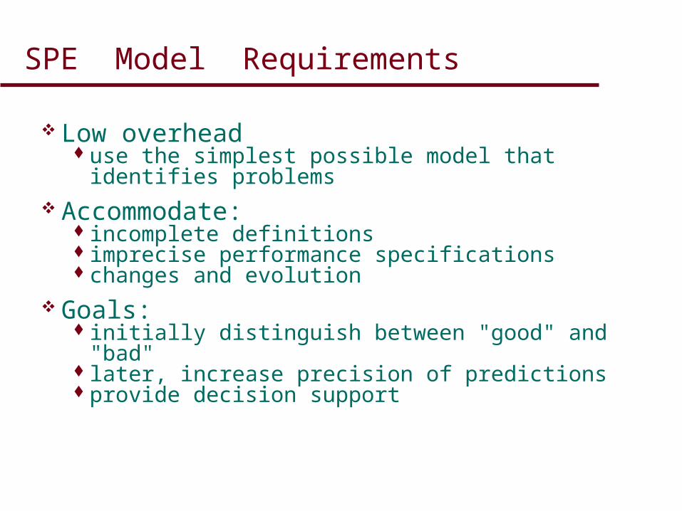
SPE Model Requirements

Low overheaduse the simplest possible model that identifies

problems Accommodate:

incomplete definitionsimprecise performance specificationschanges and evolution

Goals:initially distinguish between "good" and "bad"later, increase precision of predictions provide decision support

SPE Modeling Strategies

Simple-Model Strategystart with the simplest possible model that

identifies problems with the system architecture, design or implementation plans.

Best- and Worst-Case Strategyuse best- and worst-case estimates of resource

requirements to establish bounds on expected performance and manage uncertainty in estimates

Adapt-to-Precision Strategymatch the details represented in the models to

your knowledge of the software processing details

SPE Process Steps

1. Assess performance risk

2. Identify critical use cases

3. Select key performance scenarios

4. Establish performance objectives

5. Construct performance models

6. Determine software resource requirements

7. Add computer resource requirements

8. Evaluate the models

9. Verify and validate the models

What Do You Need To Know To Do SPE (And How Do You Get It)?

What Do You Need to Know

PerformanceObjectives

Workload Software/Database

ExecutionEnvironment

ResourceUsage

Estimates

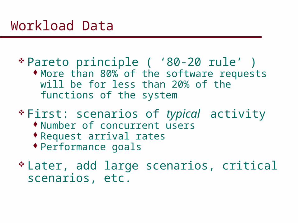
Workload Data

Pareto principle ( ‘80-20 rule’ )More than 80% of the software requests will be

for less than 20% of the functions of the system

First: scenarios of typical activityNumber of concurrent usersRequest arrival ratesPerformance goals

Later, add large scenarios, critical scenarios, etc.

Example: ATM System

System Functions:

Scenario?Scenario?

Get balance

CheckingSavings

Withdrawal

CheckingSavingsCredit card

Make payment

From checkingFrom savingsIn envelope

Deposit

SavingsChecking

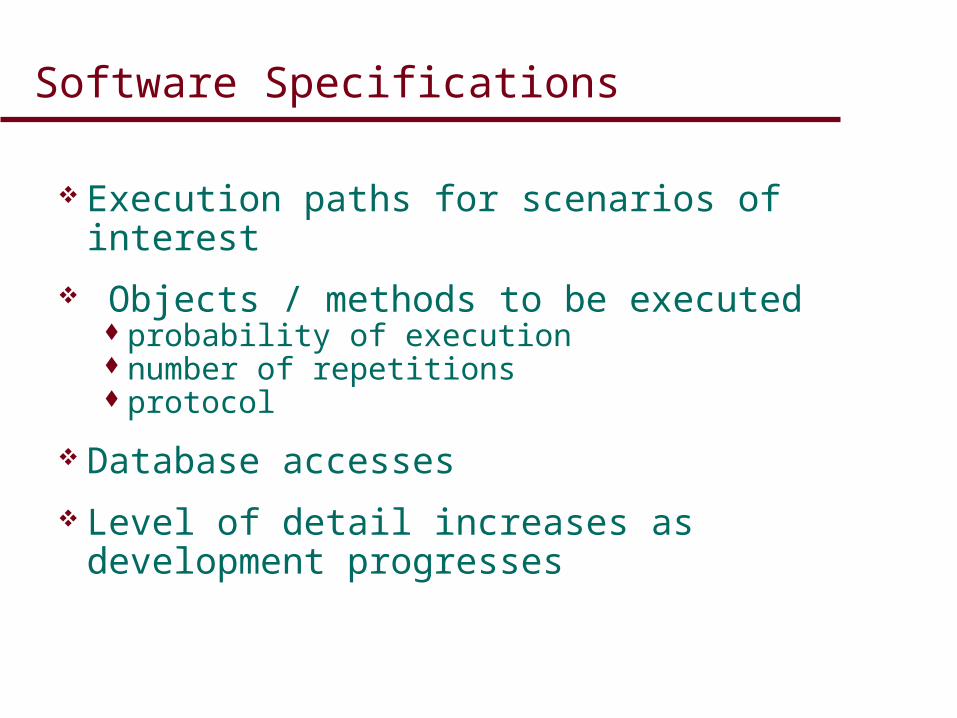
Software Specifications

Execution paths for scenarios of interest

Objects / methods to be executedprobability of executionnumber of repetitionsprotocol

Database accesses

Level of detail increases as development progresses

ATM Sequence Diagram

: User : ATM : HostBank

cardInserted

requestPIN

requestTransaction

requestAccount

requestAmount

transactionRequest

... ... ...

aPIN

response

account

amount

transactionAuthorization

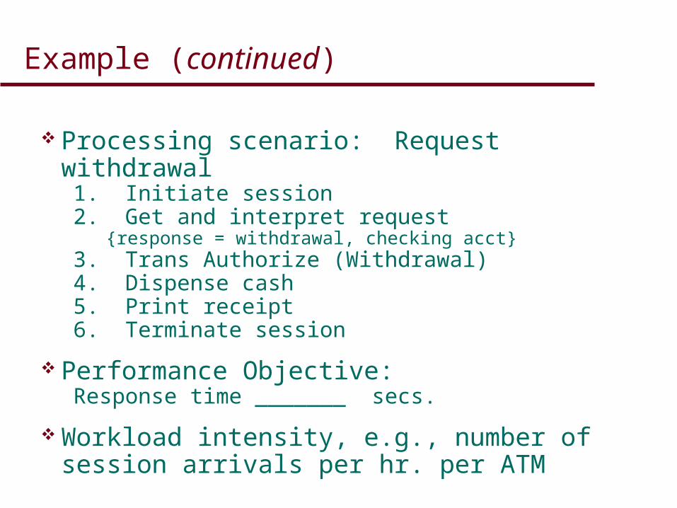
Example (continued)

Processing scenario: Request withdrawal1. Initiate session2. Get and interpret request

{response = withdrawal, checking acct}3. Trans Authorize (Withdrawal)4. Dispense cash5. Print receipt6. Terminate session

Performance Objective: Response time _______ secs.

Workload intensity, e.g., number of session arrivals per hr. per ATM

Environment

Platform and network characteristics:configurationdevice service rates

Software overhead, e.g., database path lengths, communication overhead, etc.

External factors, e.g., peak hours, bulk arrivals, batch windows, scheduling policies

Case study Environment Specifications:time for ATM communicationCPU speedsystem configuration (devices, service times,

etc.)

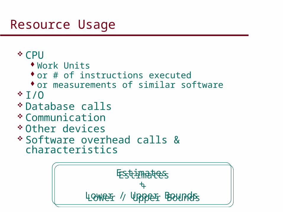
Resource Usage

CPU Work Unitsor # of instructions executedor measurements of similar software

I/O Database calls Communication Other devices Software overhead calls & characteristics

Estimates+

Lower / Upper Bounds

Estimates+

Lower / Upper Bounds

Example Specifications

initiate session

Component K Instr ATM Screens

get & interpret request

withdrawal

print balance

terminate session

200

150

250

400

100

1

0

1

0

2

2

0

1

1

dispense cash 350 1

Disk I/O’s

1

0

Sequence Diagram

: User : ATM : HostBank

cardInserted

requestPIN

aPIN

loop [until done]

requestTransaction

response

alt [type]

ref processWithdrawal

ref processDeposit

ref processBalanceInquiry

ref terminateSession

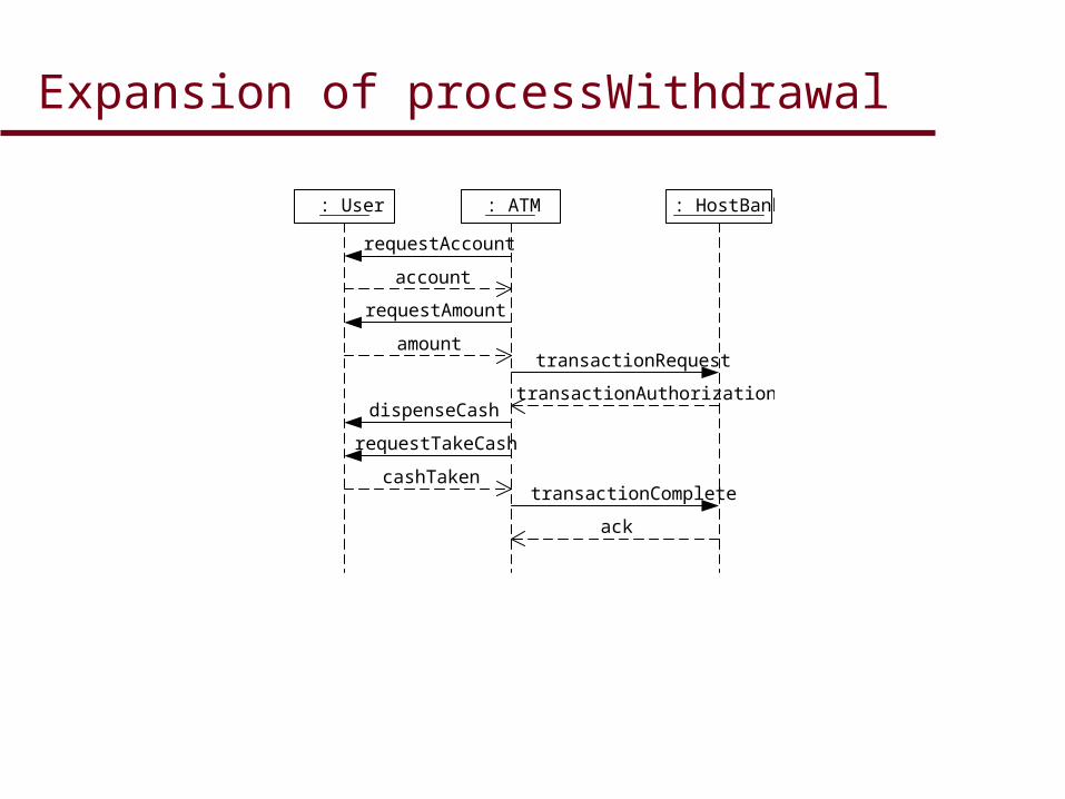
Expansion of processWithdrawal

: User : ATM : HostBank

requestAccount

requestAmount

transactionRequest

dispenseCash

requestTakeCash

transactionComplete

account

amount

transactionAuthorization

cashTaken

ack

Software Execution Model

getCardInfo

getPIN

processTransaction

terminateSession

n

getTransaction

processWithdrawal

processDeposit

processBalanceInquiry

Software Resource Requirements

getAccount

getAmount

requestAuthorization

dispenseCash

waitForCustomer

confirmTransaction

Screen 1Host 0Log 1Delay 5

Screen 0Host 0Log 0Delay 10

Screen 0Host 1Log 1Delay 0

Screen 0Host 1Log 1Delay 0

Screen 1Host 0Log 0Delay 0

Screen 1Host 0Log 0Delay 0

Computer Resource Requirements

Devices

Devices

Service Units

Screen

Host

Log

Delay

Service Time

CPU Disk Display Delay Net

1 1 1 1 1

Sec. Phys. I/O Screens Units Msgs.

0.001 1

0.005 3 2

0.001 1

1

1 0.02 1 1 0.05

Software Model Solutions

Types of solutions: Best case - shortest path in graph Worst case - longest path in graph Average Variance

Approach Repeat reduction rules on typical

structures until graph contains one node with the computed solution

Apply reductions to each resource specification (t), then combine the results

t 1

tt 2

t n

...

...

Simple Reduction Rules:Average Analysis

t1

t2

tn

t = t1 + t2 + …+ tn

n

t1

t = nt1

t0

p1

p2

t1

t2

t = t0 + p1t1 + p2t2

Lock Replace Delete Print

< 0.250

< 0.500

< 0.750

< 1.000

1.000

Resource utilization:

Model totals

0.15 CPU

0.88 ATM

1.00 DEV1

ATM example

Get cust ID from card

Get PIN from

customer

Each transaction

Get type and

process

Terminate session

Terminate session

CPU 0.00

ATM 0.03

DEV1 0.00

CPU 0.00

ATM 0.03

DEV1 0.00

CPU 0.15

ATM 0.48

DEV1 1.60

CPU 0.00

ATM 0.35

DEV1 0.00 0.00

SPE•EDTM

Display: Specify:

©1993 Performance EngineeringServices

Solve OK

Software mod Names

Results Values

Overhead Overhead

System model Service level

SPE database Sysmod globals

Save Scenario Open scenario

Solution: View:No contention Residence time

Contention Rsrc demand

System model Utilization

Adv sys model SWmod specs

Simulation data Pie chart

Results screen

Results

System Execution Model

Characterizes performance in the presence of factors that could cause contention for resources

Multiple workloads Multiple users

Provides additional information Metrics that account for resource contention Sensitivity of performance metrics to variations in

workload composition Scalability of the hardware and software The effect of new software on service level objectives of

other systems that execute on the same facility Identification of bottleneck resources Comparative data on options for improving performance

via: workload changes, software changes, hardware upgrades, and various combinations of each

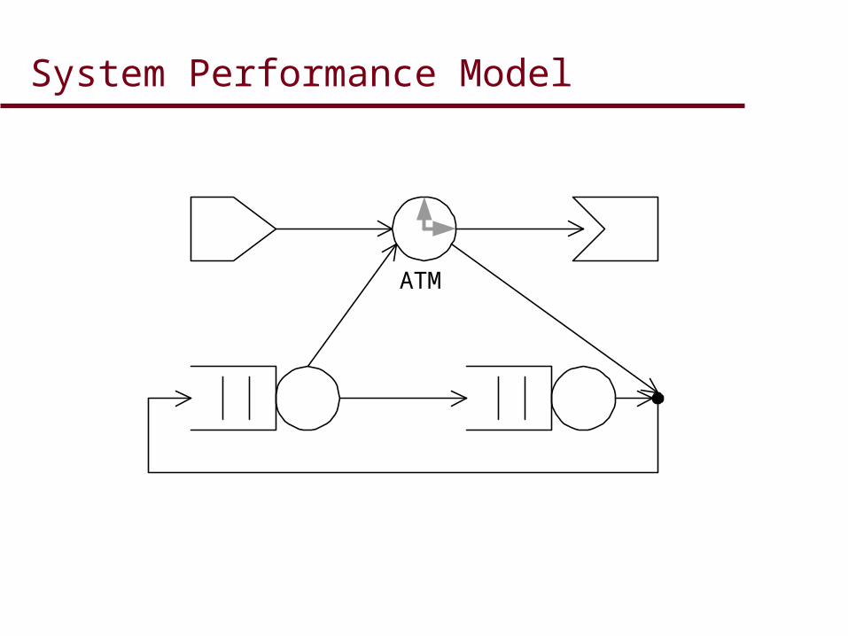
System Performance Model

ATM

System Performance Model

Lock Replace Delete PrintLock Replace Delete Print

OOD Example

< 0.250< 0.500

< 0.750

< 1.000

1.000

Utilization:

Utilization:

ATM example

0.122

0.754

0.431

0.000

Host Bank

0.12

0.430.43

Lock Replace Delete Print

< 1.250

< 2.500

< 3.750

< 5.000 5.000

Resource Usage

0.0198 CPU

21.3131 ATM

0.2060 DEV1

Residence Time: 21.5388

0.6046

0.6107

11.8527

8.4708

ATM example

Get

cust ID

Get PIN

from

Each

Get type

Termina

te

Termina

te

Lock Replace Delete Print

< 0.250

< 0.500

< 0.750

< 1.000 1.000

Resource utilization:

Model totals

0.12 CPU

0.75 ATM

0.43 DEV1

ATM example

Get

cust ID

Get PIN

from

Each

Get type

Termina

te

Termina

te

CP 0.00AT 0.02DE 0.00

CP 0.00AT 0.02DE 0.00

CP 0.12AT 0.41DE 0.43

CP 0.00AT 0.30DE 0.00 0.00

Distributed Applications

Modeling Strategy

Follow Simple-Model strategy—start with software execution model

Focus on one scenario/processor at a time

Approximate delays for communication/ synchronization with other scenarios

If the software execution model shows no problems, proceed to

System execution modelAdvanced system execution model

Partitioning the Model

Estimate theDelay for SystemInteractions

Client CPU Client Disk

N

Server CPU Server Disk

LAN

MainframeCPU

MainframeDisk(s)

n

INet

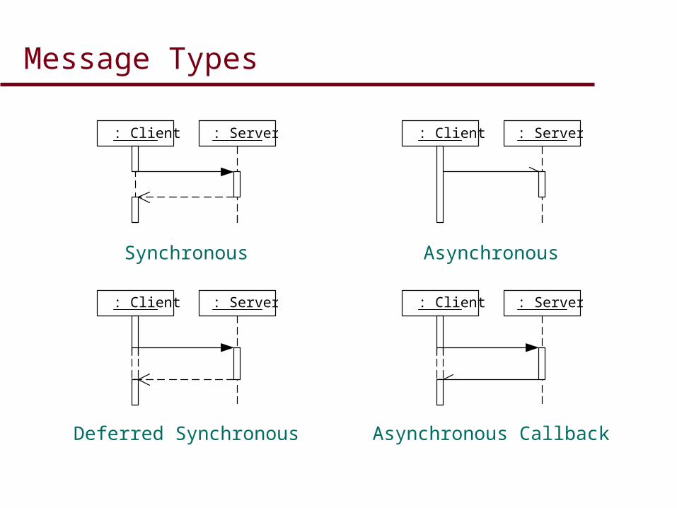
Message Types

: Client : Server : Client : Server

: Client : Server : Client : Server

Synchronous Asynchronous

Deferred Synchronous Asynchronous Callback

EG Synchronization Nodes

Reply

No reply

Synchronous call; thecaller waits for a reply

Asynchronous call;no reply

NameDeferred synchronouscall; processing occurs,wait for reply

Calling Process: Called Process:

Name

Summary

Early modeling is important for distributed systems

Use Simple-Model strategy

SPE models are straightforward to construct and solve

Performance principles, patterns and antipatterns can guide performance-oriented design