Embed Size (px)
Citation preview

1
Copepod life strategy and population viabilityin response to prey timing and temperature:Testing a new model across latitude, time,and the size spectrumNeil S. Banas 1,∗, Eva Friis Møller 2, Torkel Gissel Nielsen 3, and Lisa B.Eisner4
1Department of Mathematics and Statistics, University of Strathclyde, Glasgow, UK2Department of Bioscience, Aarhus University, Roskilde, Denmark3National Institute of Aquatic Resources, Section for Ocean Ecology and Climate,Technical University of Denmark, Charlottenlund, Denmark4NOAA Fisheries, Alaska Marine Science Center, Seattle, Washington, USACorrespondence*:Neil S. BanasDept. of Mathematics and Statistics, Univ. of Strathclyde, 26 Richmond St., GlasgowG1 1XQ, UK, [email protected]
ABSTRACT2
A new model (”Coltrane”: Copepod Life-history Traits and Adaptation to Novel Environments)3describes environmental controls on copepod populations via 1) phenology and life history and42) temperature and energy budgets in a unified framework. A set of complementary model5experiments are used to determine what patterns in copepod community composition and6productivity can be predicted from only a few key constraints on the individual energy budget: the7total energy available in a given environment per year; the energy and time required to build an8adult body; the metabolic and predation penalties for taking too long to reproduce; and the size9and temperature dependence of the vital rates involved. In an idealized global-scale testbed, the10model correctly predicts life strategies in large Calanus spp. ranging from multiple generations11per year to multiple years per generation. In a Bering Sea testbed, the model replicates the12dramatic variability in the abundance of C. glacialis/marshallae observed between warm and13cold years of the 2000s, and indicates that prey phenology linked to sea ice is a more important14driver than temperature per se. In a Disko Bay, West Greenland testbed, the model predicts the15viability of a spectrum of large-copepod strategies from income breeders with a adult size ∼ 10016µgC reproducing once per year through capital breeders with an adult size > 1000 µgC with17a multiple-year life cycle. This spectrum corresponds closely to the observed life histories and18physiology of local populations of C. finmarchicus, C. glacialis, and C. hyperboreus.19
Keywords: Zooplankton, copepod, life history, annual routine, diversity, biogeography, modelling, community ecology, Arctic20
1

Banas et al. Copepod life strategy modelling
1 INTRODUCTION
Calanoid copepods occupy a crucial position in marine food chains, the dominant mesozooplankton in21many temperate and polar systems, important to packaging of microbial production in a form accessible22to higher predators. They also represent the point at which biogeochemical processes, and numerical23approaches like NPZ (nutrient–phytoplankton–zooplankton) models, start to be significantly modulated by24life-history and behavioural constraints. The population- and community-level response of copepods to25environmental change (temperature, prey availability, seasonality) thus forms a crucial filter lying between26the biogeochemical impacts of climate change on primary production patterns and the food-web impacts27that follow.28
Across many scales in many systems, the response of fish, seabirds, and marine mammals to climate29change has been observed, or hypothesized, to follow copepod community composition more closely than30it follows total copepod or total zooplankton production. Examples include interannual variation in pollock31recruitment in the Eastern Bering Sea (Coyle et al., 2011; Eisner et al., 2014), interdecadal fluctuations in32salmon marine survival across the Northeast Pacific (Mantua et al., 1997; Hooff and Peterson, 2006; Burke33et al., 2013), and long-term trends in forage fish and seabird abundance in the North Sea (Beaugrand and34Kirby, 2010; MacDonald et al., 2015). These cases can be all be schematized as following the “junk food”35hypothesis (Osterblom et al., 2008) in which the crucial axis of variation is not between high and low total36prey productivity, but rather between high and low relative abundance of large, lipid-rich prey taxa.37
Calanoid copepods range in adult body size by more than two orders of magnitude, from<10 to>1000 µg38C. Lipid storage is likewise quite variable among species, and linked to both overwintering and reproductive39strategy (Kattner and Hagen, 2009; Falk-Petersen et al., 2009). Many but not all species enter a seasonal40period of diapause in deep water, in which they do not feed and basal metabolism is reduced to ∼1/4 of41what it is during active periods (Maps et al., 2014). Reproductive strategies include both income breeding42(egg production fueled by ingestion of fresh prey during phytoplankton blooms) and capital breeding (egg43production fueled by stored lipids in winter), as well as hybrids between the two strategies (Hirche and44Kattner, 1993; Daase et al., 2013). Generation lengths vary from several weeks to several years.45
This paper describes a numerical approach, appropriate for both regional and global scales, that predicts46many of these traits—adult size, average lipid/energy content, life cycle, and seasonal timing—from first47principles based on interactions among growth, development, reproduction, and survivorship. Our approach48draws on two currents in recent modelling work. First, it builds on the optimal annual routine approach49(McNamara and Houston, 2008) previously applied to copepods by Varpe et al. (2007, 2009) and others.50We borrow from this tradition the hypothesis, or instinct, that timing is everything in seasonal environments,51as well as the technical strategy of separately tracking structural and reserve energy stores, with the latter52variable forming a link between copepod survival strategy and the value of the copepods as prey. Second,53we embed this optimal-annual-routine logic in a trait-based metacommunity (Follows et al., 2007; Record54et al., 2013), in which a small number of traits is used to parsimoniously represent the possibility space of55“all ways there are to be a copepod.”56
The model experiments below pose the question: How many of the high-level associations among copepod57body size, body composition, generation length, reproductive strategy, and annual routine, at global or58regional scales, can be explained by a small handful of traits and tradeoffs that regulate how individual59animals best allocate energy over time? We will show that the scheme introduced here reproduces patterns60in space (large-scale trait biogeography), time (variability of one Calanus sp. in the Bering Sea), and along61
This is a provisional file, not the final typeset article 2

Banas et al. Copepod life strategy modelling
the size spectrum (differences among three coexisting Calanus spp. in Disko Bay, West Greenland), in62response to annual cycles of temperature and prey availability.63
2 MODEL DESCRIPTION
2.1 General approach64
The model introduced here is “Coltrane” (Copepod Life-history Traits and Adaptation to New65Environments) version 1.0. Like many individual-based models Fiksen and Carlotti (1998), Coltrane66represents the time-evolution of one cohort of a clonal population, all bearing the same traits and spawned67on the same date t0, with a set of ODEs. The state variables describing a cohort are relative developmental68stage D, where D = 0 represents a newly spawned egg and D = 1 an adult; survivorship N , the fraction69of initially spawned individuals that remain after some amount of cumulative predation mortality; activity70level a, 1 for normal activity and 0 for diapause; structural biomass per individual S, and “potential”71or “free scope” ϕ, which represents all net energy gain not committed to structure, i.e. a combination72of internal energy reserves and eggs already produced. Combining reserves and eggs into one pool in73this way lets us cleanly separate results that depend only on the fundamental energy budget (gain from74ingestion, loss to metabolism, and energy required to build somatic structure) from results that depend on75particular assumptions about egg production (costs, cues, and strategies). An alternate form of the model76explicitly divides ϕ into internal reserves R and income and capital egg production rates Einc and Ecap:77the simpler model without this distinction will be called the “potential” or ϕ model and the fuller version78the “egg/reserve” or ER model.79
Because our goal is to describe a broad landscape of potentially coexisting strategies rather than a single,80optimal strategy, the model is written as a family of parallel, forward-in-time integrations with traits varying81among cases, rather than using the backwards-in-time solving method of the classic optimal annual routine82approach (Houston et al., 1993; Varpe et al., 2007). The model uses a family of cases varying spawning83date t0 over the year to produce population-level results, and families of cases varying one or more traits to84produce community-level results.85
In contrast to Record et al. (2013), we do not include interactions between competing species or explicitly86resolve coexistence and its limits, keeping our representation of predation mortality simple and linear to87make this possible. The purpose of this simplification (beyond a huge increase in computational efficiency)88is to separate bottom-up from top-down mechanisms as fully as possible, for the sake of interpretability.89Record et al. (2013) show that the choice of mortality closure has a huge effect on predictions of community90structure and diversity, and this dependence can easily obscure one’s understanding of how temperature91and prey cycles affect community characteristics by themselves.92
Because we are willfully ignoring competition and coupling through predation, we will evaluate model93results in terms of the landscape of viable strategies in a given environment, rather than treating the results94as detailed predictions of relative abundance. A particular environment is defined by annual cycles of three95variables, total concentration of phytoplankton/microzooplankton prey P , surface temperature T0, and deep96temperature Td. At present, these annual cycles are assumed to be perfectly repeatable, so that a “viable”97strategy can be defined as a set of traits that lead to annual egg production above the replacement rate,98given P , T0, and Td as functions of yearday t. The effect of interannual variability on strategy is left for99future work.100
Frontiers 3
Banas et al. Copepod life strategy modelling
2.2 Time evolution of one cohort101
2.2.1 Ontogenetic development102
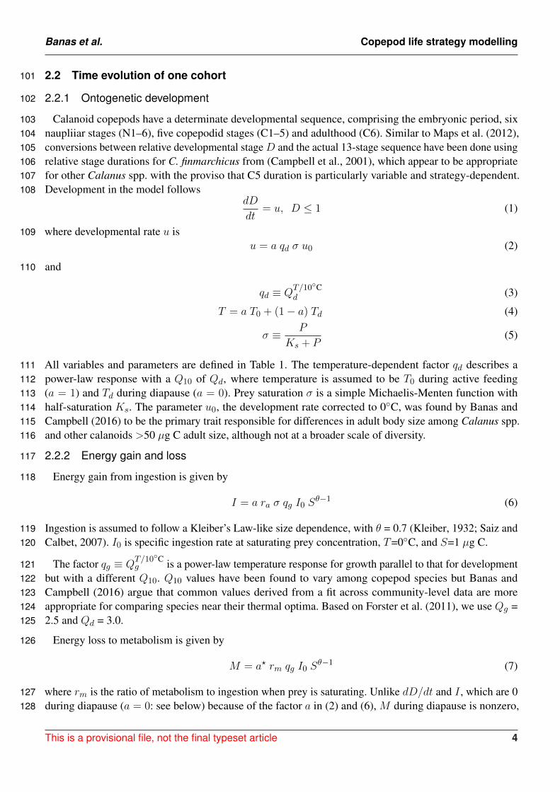
Calanoid copepods have a determinate developmental sequence, comprising the embryonic period, six103naupliiar stages (N1–6), five copepodid stages (C1–5) and adulthood (C6). Similar to Maps et al. (2012),104conversions between relative developmental stageD and the actual 13-stage sequence have been done using105relative stage durations for C. finmarchicus from (Campbell et al., 2001), which appear to be appropriate106for other Calanus spp. with the proviso that C5 duration is particularly variable and strategy-dependent.107Development in the model follows108
dD
dt= u, D ≤ 1 (1)
where developmental rate u is109u = a qd σ u0 (2)
and110
qd ≡ QT/10◦Cd (3)
T = a T0 + (1− a) Td (4)
σ ≡ P
Ks + P(5)
All variables and parameters are defined in Table 1. The temperature-dependent factor qd describes a111power-law response with a Q10 of Qd, where temperature is assumed to be T0 during active feeding112(a = 1) and Td during diapause (a = 0). Prey saturation σ is a simple Michaelis-Menten function with113half-saturation Ks. The parameter u0, the development rate corrected to 0◦C, was found by Banas and114Campbell (2016) to be the primary trait responsible for differences in adult body size among Calanus spp.115and other calanoids >50 µg C adult size, although not at a broader scale of diversity.116
2.2.2 Energy gain and loss117
Energy gain from ingestion is given by118
I = a ra σ qg I0 Sθ−1 (6)
Ingestion is assumed to follow a Kleiber’s Law-like size dependence, with θ = 0.7 (Kleiber, 1932; Saiz and119Calbet, 2007). I0 is specific ingestion rate at saturating prey concentration, T=0◦C, and S=1 µg C.120
The factor qg ≡ QT/10◦Cg is a power-law temperature response for growth parallel to that for development121
but with a different Q10. Q10 values have been found to vary among copepod species but Banas and122Campbell (2016) argue that common values derived from a fit across community-level data are more123appropriate for comparing species near their thermal optima. Based on Forster et al. (2011), we use Qg =1242.5 and Qd = 3.0.125
Energy loss to metabolism is given by126
M = a? rm qg I0 Sθ−1 (7)
where rm is the ratio of metabolism to ingestion when prey is saturating. Unlike dD/dt and I , which are 0127during diapause (a = 0: see below) because of the factor a in (2) and (6), M during diapause is nonzero,128
This is a provisional file, not the final typeset article 4

Banas et al. Copepod life strategy modelling
although reduced by a factor rb:129a? = rb + (1− rb)a (8)
In this formalism, gross growth efficiency ε can be written130
ε =I −Mr−1a I
= σra − rm (9)
We have set rm = 0.14 such that ε ≈ 0.3 when P ≈ 2Ks and ε = 0 when P = 1/4 Ks.131
2.2.3 Allocation of net gain132
Net mass-specific energy gain G is simply I −M . The two energy stores S and ϕ follow133
dS
dt= fsGS (10)
134dϕ
dt= (1− fs)GS (11)
in the case where G ≥ 0 and development is past the first feeding stage, D ≥ Df . For D < Df , we assume135G = 0 for simplicity. Positive gain is allocated between structure and potential according to the factor fs,136which commits net gain entirely to structure before a developmental point Ds, entirely to potential during137adulthood, and to a combination of them in between:138
fs =
1, D < Ds1−D1−Ds , Ds ≤ D ≤ 1
0, D = 1
(12)
When G ≤ 0, the deficit is taken entirely from reserves (eq. (11) with fs=0).139
Potential ϕ is allowed to run modestly negative, to represent consumption of body structure during140starvation conditions. A cohort is terminated by starvation if141
ϕ < −rstarvS (13)
where in this study rstarv = 0.1. A convenient numerical implementation of this scheme is to integrate S142implicitly so that it is guaranteed > 0, and to integrate ϕ explicitly so that it is allowed to change sign, with143no change of dynamics at ϕ = 0.144
2.2.4 Reserves vs. potential reserves145
If the ϕ model just described is elaborated with an explicit scheme for calculating total egg production146over time E(t), then it is possible to define R(t), individual storage/reserve biomass, and interpret R as a147state variable and ϕ as a derived quantity. The relationship between the two is148
dR
dt= (1− fs)GS − E (14)
ϕ(t) = R(t) +
∫ t
t0
E(t′) dt′ (15)
Frontiers 5

Banas et al. Copepod life strategy modelling
Thus ϕ tracks the reserves that an animal would have remaining if it had not previously started egg149production. This is a useful metric for optimising reproductive timing, as we will show (Section 2.3).150
2.2.5 Predation mortality151
Predation mortality is assumed to have the same dependence on temperature and body size as ingestion,152metabolism, and net gain (Hirst and Kiørboe, 2002). Survivorship N is set to 1 initially and decreases153according to154
d(lnN)
dt= −m (16)
where155m = a qg S
θ−1 m0 (17)
so that predation pressure relative to energy gain is encapsulated in a single parameter m0. In practice m0156is a tuning parameter but we can solve for the value that would lead to an approximate equilibrium between157growth and mortality. Solving for158
1
NS
d(NS)
dt= 0 (18)
after some algebra yields m = fsG, and with a = 1 this becomes159
m0
I0= εfs (19)
Averaging fs over the maturation period 0 ≤ D ≤ 1 with Ds = 0.35 and assuming ε ≈ 0.3 gives160m0/I0 = 0.2. This is the default level of predation in the model except where otherwise specified.161
2.2.6 Activity level and diapause162
Modulation of activity level a has been treated as simply as possible, using a “myopic” criterion that163considers only the instantaneous energy budget, rather than an optimisation over the annual routine164or lifetime (Sainmont et al., 2015). Furthermore, we treat a as a binary switch—diapause or full165foraging activity—although intermediate overwintering states have been sometimes observed, e.g., C.166glacialis/marshallae on the Eastern Bering Sea shelf in November (R. G. Campbell, pers. comm.), and167a continuously varying a could be used to represent modulations in diel vertical migration or foraging168strategy more generally. In the present model, we set a = 0 if D > Ddia (the stage at which diapause first169becomes possible) and prey saturation σ is below a threshhold σcrit, and set a = 1 otherwise. The prey170saturation threshhold is determined by maximising the rate of total population energy gain as a function of171a. When d/da of this quantity is positive, active foraging a = 1 is the optimal instantaneous strategy and172when it is negative, a = 0 is optimal. I.e., the threshhold173
d
da
d
dt(ϕ+ S)N = 0 (20)
can be rearranged to give174
σcrit =rm(1− rb)
ra+Cdiara
m0
I0(21)
where Cdia = 1+ϕ/S. The first term in (21) can be derived more simply by setting dG/da = 0, a criterion175based on ingestion and metabolism alone. The second term adjusts this criterion by discouraging foraging176at marginal prey concentrations when predation is high. This second term, however, tends to produce177
This is a provisional file, not the final typeset article 6

Banas et al. Copepod life strategy modelling
unrealistic, rapid oscillations in which the copepods briefly “top up” on prey and then hide in a brief178“diapause” to burn them: this is the limitation of a myopic criterion in which diapause is not explicitly179required to be seasonal, and of combining actual lipid reserves and potential egg production into a single180state variable. Pragmatically, the issue can be eliminated by replacing Cdia with 1 + R/S; or, to preserve181the self-sufficiency of the ϕ model, by approximating Cdia as182
Cdia = max[0, 1 + min
(rmaxϕ ,
ϕ
S
)](22)
where rmaxϕ = 1.5.183
2.3 Population-level response184
The viability of a trait combination in a given environment can be expressed in terms of the egg fitness F ,185future egg production per egg (Varpe et al., 2007). F depends on spawning timing t0, which we assume186a copepod population is completely free to optimise: we do not impose any constraints representing187environmental cues or additional physiological requirements. The approach to optimising t0 and solving188for F differs between the ϕ and ER versions of the model, which we will discuss separately. However, both189methods require an estimate of individual egg biomass We in order to convert ϕ(t) or E(t) from carbon190units into a number of eggs, and so a digression on the determination of We is required.191
2.3.1 Egg and adult size192
The problem of estimating We can be replaced by the problem of estimating adult size Wa using the193empirical relationship for broadcast spawners determined by Kiørboe and Sabatini (1995):194
lnWe ≈ ln rea + θea lnWa (23)
where rea = 0.013, θea = 0.62. (In the ER model, Wa ≡ S + R at D = 1, but in the ϕ model we195approximate it as S alone for simplicity.) Adult size itself is an important trait for the model to predict, but196the controls on it are rather buried in the model formulation above. Banas and Campbell (2016) describe a197theory relating body size to the ratio of development rate to growth rate based on a review of laboratory198data for copepods with adult body sizes 0.3–2000 µgC. In our notation, their model can be derived as199follows: if we approximate (10), (11) in terms of a single biomass variable as200
dW
dt= ε′ qg I0 W
θ, D ≥ Df (24)
then integrating from spawning to maturation gives201
1
1− θW 1−θ
∣∣∣∣D=1
D=0
= (1−Df ) ε′ qg I01
u(25)
since u is the reciprocal of the total development time. Growth rate has been written in terms of I0 and an202effective growth efficiency over the development period ε′. If we assume that egg biomass We = W |D=0 is203much smaller than Wa = W |D=1, then combining (25) with (2) gives204
Wa ≈
[(1− θ) (1−Df ) ε′
(QgQd
)T/10◦CI0u0
] 11−θ
(26)
Frontiers 7
Banas et al. Copepod life strategy modelling
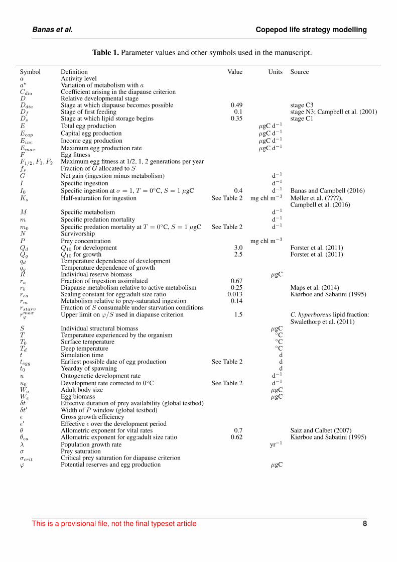
Table 1. Parameter values and other symbols used in the manuscript.
Symbol Definition Value Units Sourcea Activity levela? Variation of metabolism with aCdia Coefficient arising in the diapause criterionD Relative developmental stageDdia Stage at which diapause becomes possible 0.49 stage C3Df Stage of first feeding 0.1 stage N3; Campbell et al. (2001)Ds Stage at which lipid storage begins 0.35 stage C1E Total egg production µgC d−1Ecap Capital egg production µgC d−1Einc Income egg production µgC d−1Emax Maximum egg production rate µgC d−1F Egg fitnessF1/2, F1, F2 Maximum egg fitness at 1/2, 1, 2 generations per yearfs Fraction of G allocated to SG Net gain (ingestion minus metabolism) d−1I Specific ingestion d−1I0 Specific ingestion at σ = 1, T = 0◦C, S = 1 µgC 0.4 d−1 Banas and Campbell (2016)Ks Half-saturation for ingestion See Table 2 mg chl m−3 Møller et al. (????),
Campbell et al. (2016)M Specific metabolism d−1m Specific predation mortality d−1m0 Specific predation mortality at T = 0◦C, S = 1 µgC See Table 2 d−1N SurvivorshipP Prey concentration mg chl m−3Qd Q10 for development 3.0 Forster et al. (2011)Qg Q10 for growth 2.5 Forster et al. (2011)qd Temperature dependence of developmentqg Temperature dependence of growthR Individual reserve biomass µgCra Fraction of ingestion assimilated 0.67rb Diapause metabolism relative to active metabolism 0.25 Maps et al. (2014)rea Scaling constant for egg:adult size ratio 0.013 Kiørboe and Sabatini (1995)rm Metabolism relative to prey-saturated ingestion 0.14rstarv Fraction of S consumable under starvation conditionsrmaxϕ Upper limit on ϕ/S used in diapause criterion 1.5 C. hyperboreus lipid fraction:
Swalethorp et al. (2011)S Individual structural biomass µgCT Temperature experienced by the organism ◦CT0 Surface temperature ◦CTd Deep temperature ◦Ct Simulation time dtegg Earliest possible date of egg production See Table 2 dt0 Yearday of spawning du Ontogenetic development rate d−1u0 Development rate corrected to 0◦C See Table 2 d−1Wa Adult body size µgCWe Egg biomass µgCδt Effective duration of prey availability (global testbed)δt′ Width of P window (global testbed)ε Gross growth efficiencyε′ Effective ε over the development periodθ Allometric exponent for vital rates 0.7 Saiz and Calbet (2007)θea Allometric exponent for egg:adult size ratio 0.62 Kiørboe and Sabatini (1995)λ Population growth rate yr−1σ Prey saturationσcrit Critical prey saturation for diapause criterionϕ Potential reserves and egg production µgC
This is a provisional file, not the final typeset article 8

Banas et al. Copepod life strategy modelling
Properly speaking, both ε′ and T in (26) are functions of t0 since they depend on the alignment of the205development period with the annual cycle. Since we are trying to use (23) and (26) to optimise t0, we206have a circular problem. Record et al. (2013) derive an expression similar to (26) and apply it iteratively207because of this circularity. Some applications of Coltrane might require the same level of accuracy, but in208the present study we take the expedient approach of simply assuming that T is the annual mean of T0 and209that ε′ ≈ 1/3: i.e., that after t0 is optimised, some diapause/spawning strategy will emerge that aligns the210maturation period moderately well with a period of high prey availability. This assumption eliminates the211need to run the model before estimating We via (23) and (26).212
2.3.2 Optimal timing in the ϕ model213
With a method for approximating We in hand, we can define egg fitness F as a function of ϕ. If a cohort214spawned on t0 were to convert all of its accumulated free scope ϕ—all net energy gain beyond that required215to build an adult body structure—into eggs on a single day t1, the eggs produced per starting egg would be216
F (t0 → t1) =ϕ(t1)
WeN(t1) (27)
This expression condenses one copepod generation into a mapping F similar to the “circle map” of Gurney217et al. (1992). Once the ODE model has been run for a family of t0 cases, this mapping can be used to218quickly identify optimal life cycles of any length. The optimal one-generation-per-year strategy is the t0219that maximizes F1 = F (t0 → t0 + 365). The optimal one-generation-per-two-years strategy has t0 that220maximizes F1/2 = F (t0 → t0 + 2 · 365). The optimal two-generation-per-year strategy has spawning dates221t0, t1 that maximize the product F2 = F (t0 → t1) · F (t1 → t0 + 365); and so on. A viable strategy is a222combination of spawning dates and model parameters that give F ≥ 1.223
2.3.3 Optimal timing in the ER model224
In reality, of course, copepods are not free to physically store indefinite amounts of reserves within225their bodies and then instantaneously convert them into eggs when the timing is optimal. If a scheme for226calculating egg production over time E(t) is added to the model (and note that this scheme has not yet227been specified in our discussion), then the per-generation mapping represented by F takes a different form.228First, we use the assumption that the environmental annual cycle repeats indefinitely to convert the time229series of EN—egg production discounted by survivorship—from a function of days since spawning to a230function of yearday. By combining time series of EN/We from a family of cases varying t0, we construct231a transition matrix V that gives eggs spawned on each yearday in generation k + 1, given eggs per yearday232in generation k:233
nk+1 = V · nk (28)
where n is a discrete time series spanning one year (in practice we discretize the year into 5 d segments234rather than yeardays per se). The first eigenvector of V then gives a seasonal pattern of egg production235that is stable in shape, with the corresponding eigenvalue λ giving one plus the population growth rate per236generation: nk+1(t) = V · nk(t) = λ · nk(t). A strict criterion for strategy viability would then be λ ≥ 1,237although this criterion is unhelpfully sensitive to predation mortality. A more robust criterion (which we238use in Section 3.4 below) is to consider a strategy viable if it yields lifetime egg production above the239replacement rate: if E(t0; t) and N(t0; t) are the time series of egg production and survivorship for a cohort240
Frontiers 9

Banas et al. Copepod life strategy modelling
spawned on t0, and n(t0) is a normalized annual cycle of egg production,241 ∫ 365
0
∫ ∞0
n(t0)E(t0; t)N(t0; t)
Wedt dt0 ≥ 1 (29)
Thus in the ER version of the model, as in the ϕ version, we have an efficient method that describes the242long-term viability of a trait combination under a stable annual cycle, along with the optimal spawning243timing associated with those traits in that environment; and these methods only require us to explicitly244simulate one generation.245
2.4 Assembling communities246
Community-level predictions in Coltrane take the form of bounds on combinations of traits that lead to247viable populations in a given environment. There are many copepod traits represented in the model that one248might consider to be axes of diversity or degrees of freedom in life strategy: u0, I0, θ, Ds, Ks, We/Wa,249and even m0 to the extent that predation pressure is a function of behaviour (Visser et al., 2008). Record250et al. (2013) allowed five traits to vary among competitors in their copepod community model. We have251taken a minimalist approach, where in the ϕ model we allow only one degree of freedom: variation in u0252from 0.005–0.01 d−1. Banas and Campbell (2016) showed from a review of lab studies that u0 variations253appear to be the primary mode of variation in adult size among large calanoids (Wa > 50 µgC) including254Calanus and Neocalanus spp., with slower development leading to larger adult sizes. That study also255suggests that variation in I0 is responsible for copepod size diversity on a broader size or taxonomic scale256(e.g. between Calanus and small cyclopoids like Oithona). However, variation in I0 (energy gain from257foraging) probably only makes sense as part of a tradeoff with predation risk or egg survivorship (Kiørboe258and Sabatini, 1995) and we have left the formulation of that tradeoff for future work. We therefore expect259Coltrane 1.0 to generate analogs for large and small Calanus spp. (∼100–1000 µgC adult size) but not260analogs for Oithona spp. or even small calanoids like Pseudocalanus or Acartia.261
Choices regarding reproductive strategy require another degree of freedom. In the ϕ model, this does262not require additional parameters, because the difference between, e.g., capital spawning in winter and263income spawning in spring is simply a matter of the time t at which F is evaluated in postprocessing: each264model run effectively includes all timing possibilities (eq. (27)). In the ER model, however, diversity in265reproductive timing must be made explicit. In the one experiment below that uses the ER model (Section2663.4), we use the following scheme for egg production. E(t) is the sum of income egg production Einc267and capital egg production Ecap, which are 0 until maturity is reached (D = 1) and an additional timing268threshhold has been passed (t > tegg). Past those threshholds, they are calculated as Einc = G if G > 0269and Ecap = Emax − Einc if R > 0, where Emax is a maximum egg production rate which we assume270to be equal to the food-saturated ingestion rate ra qg I0 Sθ. Thus the trait tegg determines whether egg271production begins immediately upon maturation or after some additional delay. Instead of tegg, expressed272in terms of calendar day, one could introduce the same timing freedom through a trait linked to light, an273ontogenetic clock that continues past D = 1, or a more subtle physiological scheme. However, since we274run a complete spectrum of trait values in each environmental case, it is not important to the results how the275delay is formulated, provided we only compare model output, rather than actual trait values, across cases.276
2.5 Model experiments277
This study comprises three complementary experiments (Table 2). The first of these is an idealized278global testbed which addresses broad biogeographic patterns. The second is a testbed representing the279
This is a provisional file, not the final typeset article 10

Banas et al. Copepod life strategy modelling
Table 2. Setup of model experiments. All other parameters are as in Table 1.
Experiment Environmental forcing Variable traits Ks m0 Model
Global Surface, deep temperatures u0 = 0.005 – 0.01 d−1 1 mg chl m−3 0.08 d−1 ϕconstant; Gaussian windowof prey availability
Bering Family of seasonal cycles u0 = 0.007 d−1 3 0.08 ϕon the middle shelf:see Appendix
Disko One seasonal cycle (1996–97): u0 = 0.005 – 0.01 d−1, 1 0.06 ERsee Appendix tegg = 0 – 1095
Eastern Bering Sea shelf, which addresses time-variability in one population in one environment. The last280is a testbed representing Disko Bay, West Greenland, which addresses trait relationships along the size281spectrum in detail. The first two are evaluated entirely in terms of the ϕ model, while in the Disko Bay282case we use the ER model to allow more specific comparisons with observations.283
The global testbed consists of a family of idealized environments in which surface temperature T0 is held284constant, and prey availability is a Gaussian window of width δt′ centered on yearday 365/2:285
P (t) = (10 mg chl m−3) exp
− (t− 3652
δt′
)2 (30)
We assume that deep, overwintering temperature Td = 0.4 T0. The ratio 0.4 matches results of a regression286between mean temperature at 0 and 1000 m in the Atlantic between 20–90◦N, or 0 and 500 m in the Pacific287over the same latitudes (World Ocean Atlas 2013: http://www.nodc.noaa.gov/OC5/woa13/). We compare288environmental cases in terms of T0 and an effective season length δt =
∫σ dt, which rescales the δt′ cases289
in terms of the equivalent number of days of saturating prey per year.290
The Bering Sea testbed considers interannual variation in temperature, ice cover, and the effect of ice291cover on in-ice and pelagic phytoplankton production (Stabeno et al., 2012b; Sigler et al., 2014; Banas292et al., 2016). Variation between warm, low-ice years and cold, high-ice years has previously been linked to293the relative abundance of large zooplankton including Calanus glacialis/marshallae (Eisner et al., 2014),294and we test Coltrane predictions against 8 years of C. glacialis/marshallae observations from the BASIS295program. Seasonal cycles of T0, Td, and P are parameterized using empirical relationships between ice296and phytoplankton from Sigler et al. (2014) and a 42-year physical hindcast using BESTMAS (Bering297Ecosystem Study Ice-ocean Modeling and Assimilation System: Zhang et al. (2010); Banas et al. (2016)).298Details are given in the Appendix.299
The Disko Bay testbed represents one seasonal cycle of temperature and phytoplankton and300microzooplankton prey, based on the 1996–97 time series described by Madsen et al. (2001). We use301this particular dataset not primarily as a guide to the current or future state of Disko Bay but rather as a302specific circumstance in which the life-history patterns of three coexisting Calanus spp. (C. finmarchicus,303C. glacialis, C. hyperboreus) were documented (Madsen et al., 2001). Details are given in Section 3.4 and304the Appendix.305
Frontiers 11

Banas et al. Copepod life strategy modelling
3 RESULTS
3.1 An example population306
One case from the global experiment with u0 = 0.007 d−1, T0 = 1◦C, and δt = 135 is shown in detail in307Fig. 2 to illustrate the analysis method described in Section 2.3.2. In this case, out of cohorts spawned over308the full first year, only those spawned in spring reached adulthood without starving (Fig. 2b, blue–green309lines; non-viable cohorts not shown). The fitness function F (eq. 27) declines during winter diapause and310rises during the following summer when prey are available. There is no equivalent peak during the third311summer, indicating that by this time cumulative predation mortality is so high that there is no net advantage312to continuing to forage before spawning.313
The maximum value of F for most cohorts (?, Fig 2c) comes at ∼1.5 yr into the simulation, at the peak314in prey availability following maturation. This point in the annual cycle, however, does not fall within the315window of spawning dates at which maturation is possible (compare year 2 in Fig. 2c with year 1 in Fig.3162b), and thus is an example of “internal life history mismatch” (Varpe et al., 2007), the common situation317in which the spawning timing that maximizes egg production by the parent is not optimal for the offspring.318The long-term egg fitness corresponding to stable 1-year and 2-year cycles is marked for each cohort (Fig.3192c, red, orange circles). Some but not all of the cohorts that reach maturity are able to achieve F > 1,320egg production above the replacement rate, in these cyclical solutions (solid circles). The best one-year321and two-year strategies achieve similar maximum fitness values (red vs. orange solid dots), although they322require slightly different seasonal timing.323
3.2 Global behaviour324
In the global experiment, populations like that shown in Fig. 2 were run for a spectrum of u0 values,325across combinations of T0 and δt from -2–16◦C and 0–310 d (the latter corresponding to δt′ from 0–150326d). Across these cases, at a given u0, the model predicts a log-linear relationship between adult size and327temperature, which is not much perturbed by variation in prey availability (Fig. 3). The slope of this328relationship is equivalent to a Q10 of 1.8–2.0, significantly steeper than the size dependence explicitly329imposed by the growth/development parameterization (Qd/Qg = 1.2; eq. 26). This suggests that not only330physiological mechanisms (Forster and Hirst, 2012) but additional, emergent, ecological mechanisms are331contributing. Provocatively, a similar contrast exists between laboratory measurements of temperature332dependence in C. finmarchicus (Qd/Qg = 1.3, Campbell et al. (2001)) and field observations of size in333relation to temperature in C. finmarchicus and C. helgolandicus across the North Atlantic (Q10 = 1.65,334Wilson et al. (2015), with prosome length converted to carbon weight based on Runge et al. (2006)).335
The intercept of the size-temperature relationship depends on u0 (Fig. 3), with u0 = 0.005–0.01 d−1336corresponding to the range of adult size from C. finmarchicus to C. hyperboreus at the cold end of the337temperature spectrum (Disko Bay, ∼ 0◦C: Swalethorp et al. (2011)). It is not always fair, however, to338associate a particular u0 value with a particular species over the full range of temperatures included. As339Banas and Campbell (2016) discuss further, the temperature response of an individual species is often340dome-shaped, a window of habitat tolerance (Møller et al., 2012; Alcaraz et al., 2014), whereas Coltrane3411.0 uses the monotonic, power-law response observable at the community level (Forster et al., 2011)). C.342finmarchicus, for example, is fit well by u0 = 0.007 d−1 at higher temperatures (4–12◦C), whereas near3430◦C in Disko Bay, it has been observed to be considerably smaller than extrapolation along the u0 = 0.007344d−1 power law would predict. Past studies have also found C. finmarchicus growth and ingestion to be345
This is a provisional file, not the final typeset article 12

Banas et al. Copepod life strategy modelling
suppressed at low temperatures, i.e., to show a very high Q10 compared with the community-level value346(Campbell et al., 2001; Møller et al., 2012).347
With this caveat on the interpretation of u0, we can observe a sensible gradation in life strategy along the348u0 axis (Fig. 4). From u0 = 0.01 d−1 (C. finmarchicus-like at 0◦C) to u0 = 0.005 d−1 (C. hyperboreus-like),349the environmental window in which multi-year life cycles are viable (F1/2 ≥ 1) expands dramatically.350This window overlaps significantly with the window of viability for one-year life cycles (F1 ≥ 1; Fig. 4,351black vs. gray contours). In all u0 cases, there is a non-monotonic pattern in maximum fitness as a function352of either temperature or prey (Fig. 4, color contours), as environments align and misalign with integer353numbers of generations per year or years per generation.354
The number of generations per year in the timing strategy that optimizes F for each (T0, δt) habitat355combination is shown in Fig. 5 for u0 = 0.007 d−1. This u0 value corresponds in adult size to Arctic C.356glacialis and temperate C. marshallae populations in the Pacific (Fig. 3), species which coexist and are357nearly indistinguishable in the Bering Sea. In the lowest-prey conditions, no timing strategy is found to358be viable. As prey and temperature increase, the model predicts bands proceeding monotonically from359multiple years per generation to multiple generations per year. Validating these model predictions requires360parameterizing places (in terms of T0 and δt) in addition to parameterizing their inhabitants, and thus the361meaning of either success of failure is ambiguous. Still, we can observe the following. Ice Station Sheba in362the high Pacific Arctic (Fig. 1) falls in the non-viable regime (Fig. 5), consistent with the conclusion of363Ashjian et al. (2003) that Calanus spp. are unable to complete their life cycle there. Disko Bay falls on364the boundary of one- and two-year generation lengths, consistent with observations of C. glacialis there365(Madsen et al., 2001). At Newport, Oregon, near the southern end of the range of C. marshallae, the model366predicts multiple generations per year, consistent with observations by Peterson (1979).367
3.3 A high-latitude habitat limit in detail: The Eastern Bering Sea368
These idealized experiments (Figs. 4,5) suggest that very short productive seasons place a hard limit369on the viability of Calanus spp., regardless of size, temperature, generation length, or match/mismatch370considerations (although these factors affect where exactly the limit falls). A decade of observations in the371Eastern Bering Sea provide a unique opportunity to resolve this viability limit with greater precision. This372analysis takes advantage of the natural variability on the Southeastern Bering Sea shelf described by the373“oscillating control hypothesis” of Hunt et al. (2002, 2011): in warm, low-ice years, the spring bloom in374this region is late (∼ yearday 150: Sigler et al. (2014)) and the abundance of large crustacean zooplankton375including C. glacialis/marshallae is very low, while in colder years with greater ice cover, the pelagic376spring bloom is earlier, ice algae are present in late winter, and large crustacean zooplankton are much377more abundant. The task of replicating these observations serves to test the Coltrane parameterization, and378situating them within a complete spectrum of temperature/ice cover cases also allows the model to provide379some insight into mechanisms.380
Mean surface temperature T0 was used to index annual cycles of surface and bottom temperature on the381Eastern Bering Sea middle shelf (Appendix; insets in Fig. 6). Date of ice retreat tice was likewise used382to index phytoplankton availability over each calendar year (Appendix; insets in Fig. 6). Coltrane was383run for each (T0, tice) combination with u0 = 0.007 d−1, thus consistent with Fig. 5 except for the more384refined treatment of environmental forcing, and an adjustment to Ks to match results of Bering Sea feeding385experiments (Campbell et al., 2016)). The maximum egg fitness F for a one-generation-per-year strategy is386shown as a function of T0 and tice in the main panel of Fig. 6. Coltrane predicts that one generation per387year is the optimal life cycle length everywhere in this parameter space except for the cold/ice-free and388
Frontiers 13

Banas et al. Copepod life strategy modelling
warm/high-ice-cover extremes (white contours), combinations which do not occur anywhere in a hindcast389of middle-shelf conditions back to 1971 (Fig. 6, red and blue dots).390
Late summer measurements of C. glacialis/marshallae abundance (individuals m−2), averaged over the391middle/outer shelf south of 60◦N, are shown in Fig. 6 for 2003–2010 (n=364 over the 8 years; Eisner392et al. (2014)). Both these observations and the predicted maximum F from Coltrane show a dramatic393contrast between the warm years of 2003–05 (tice = 0) and the cold years of 2007–10 (tice=100–130),394with the transitional year 2006 harder to interpret. Eisner et al. (2014) found that there was less contrast395between cold year/warm year abundance patterns on the northern middle/outer shelf, consistent with the396model prediction that all hindcast years on the northern shelf fall within the “viable” habitat range for C.397glacialis/marshallae (Fig. 6, blue dots).398
The viability threshhold that the Southeastern Bering Sea appears to straddle is qualitatively similar399to that in the more idealized global experiment (Figs. 5,4), primarily aligned with the phenological400index (horizontal axis) rather than the temperature index (vertical axis). The threshhold in the Bering401Sea experiment falls somewhat beyond the dividing line imposed in the experiment setup between early,402ice-retreat-associated blooms and late, open-water blooms (tice = 75: see Appendix, Sigler et al. (2014)).403This gap (whose width depends on the mortality level m0: not shown) indicates that some period of ice404algae availability is required by C. glacialis/mashallae in this system, in addition to a favorable pelagic405bloom timing.406
3.4 Coexisting life strategies in detail: Disko Bay407
The experiments above test the ability of Coltrane 1.0 to reproduce first-order patterns in latitude and time408but do not provide sensitive tests of the model biology. A model case study in Disko Bay, where populations409of three Calanus spp. coexist and have been described in detail (Madsen et al., 2001; Swalethorp et al.,4102011), allows a closer examination of the relationships among traits within the family of viable life411strategies predicted by Coltrane.412
The model forcing (Fig. 7 describes a single annual cycle, starting with the 1996 spring bloom. This413represents a cold, high-ice state of the system, compared with more recent years in which the spring bloom414is earlier (e.g. 2008, Fig. 7, Swalethorp et al. (2011)) and the deep layer is warmed by Atlantic water415intrusions (Hansen et al., 2012). This particular year was chosen because measurements of prey availability416and Calanus response by Madsen et al. (2001) were particularly complete and coordinated. A simple417attempt to correct the prey field for quality and Calanus preference was made by keeping only the >11 µm418size fraction of phytoplankton and adding total microzooplankton, in µg C. The measured phytoplankton419C:chl ratio was used to convert the sum to an equivalent chlorophyll concentration, and this time series was420then slightly idealized for clarity (Fig. 7, Appendix).421
Sensible results were only possible after tuning the predation mortality scale coefficient m0. It is likely422that our simple mortality scheme introduces some form of bias, compared with the reality in this system of423predation by successive waves of visual and non-visual predators, which will be considered in a separate424study. Still, a sensitivity experiment using the ϕ model shows that varying m0 has, as intended, a simple,425uniform effect on fitness/population growth (Fig. 8) that leaves other trait relationships along the size426spectrum unaffected. The ϕ model predicts that copepods similar to C. finmarchicus in size have much427greater fitness at a generation length of one year than at two years or more; that C. hyperboreus would be428unable to complete its life cycle in one year, but is well-suited to a two-year cycle; and that C. glacialis429falls in the size range where one- and two-year life cycles have comparable fitness value. These results are430
This is a provisional file, not the final typeset article 14

Banas et al. Copepod life strategy modelling
consistent with observations (Madsen et al., 2001) and more general surveys of life strategies in the three431species (Falk-Petersen et al., 2009; Daase et al., 2013).432
For greater specificity, we switched from the ϕ to the ER model version, running a spectrum of tegg cases433(see section 2.4) along with a spectrum of u0 cases. The ER model imposes additional constraints on the434model organisms—e.g., they are no longer allowed an infinite egg production rate—and to compensate we435reduced m0 from 0.08 d−1 to 0.06 d−1. The relationship between generation length and adult size across all436(u0, tegg) combinations is shown in Fig. 9. Results are consistent with the ϕ model (Fig. 8): only a one-year437life cycle is viable for C. finmarchicus in this environment, only a two-year or longer cycle is viable for C.438hyperboreus, and C. glacialis again lies near the boundary where the two strategies are comparable.439
The ER model predicts a time series of egg production associated with each trait combination, not just440an optimal date (Section 2.3.3), and compositing these over all viable cases within 30% of the average441measured adult size for each species allows us to compare modelled egg production patterns directly with442observations. The model predicts that C. finmarchicus analogs spawn in close association with the spring443bloom, that C. hyperboreus spawns well before the spring bloom, and that C. glacialis is intermediate444(Fig. 10, Fig. 11a). These patterns are all in accordance with Disko Bay observations (Madsen et al., 2001;445Swalethorp et al., 2011), although the absolute range is muted: Madsen et al. (2001) report C. hyperboreus446spawning as early as February. As one would expect from these timing patterns, the model predicts a447significant trend between size and the capital fraction of total egg production Ecap/(Einc+Ecap) (Fig. 11c).448Again, the pattern is qualitatively correct but muted: Coltrane predicts 80% income breeding at the size of449C. finmarchicus (a pure income breeder in reality) and 80% capital breeding at the size of C. hyperboreus (a450pure capital breeder in reality). More notable than the error is how much of the income/capital spectrum can451apparently be reproduced as a consequence of optimal timing alone, without imposing the physiological452difference between the two strategies as an independent trait (Ejsmond et al., 2015).453
The model predicts (Fig. 11b) that the largest model organisms, with the longest generation lengths, enter454their first diapause near the boundary between copepodite stages C4 and C5 (D ≈ 0.75), whereas smaller455organisms enter first diapause well into stage C5. Madsen et al. (2001) found that both C. glacialis and456C. hyperboreus diapause as C4, C5, and adults in Disko Bay, suggesting that the model is biased toward457fast maturation. The discrepancy could also be related to intraspecific variation in the real populations458or non-equiproportional development in the late stages, i.e., a variable conversion scale between actual459developmental stage and D.460
Finally, the ER version of Coltrane allows an estimate of the fraction of individual carbon in the form of461storage lipids R/(R+ S) (Fig. 11d). Averaging each model population from D = Ddia through adulthood,462weighted by survivorship N , yields an overall range that compares well with the species-mean wax ester463fractions measured by Swalethorp et al. (2011): ∼30% for C. finmarchicus to ∼60% for C. hyperboreus.464In the middle of the size spectrum, reserve fraction is highly variable across viable two-year strategies, a465warning that the success of this final model prediction may be partly fortuitous. Still, taken as a whole,466this experiment has yielded a striking result: that a small set of energetic and timing contraints is able to467correctly predict, a priori, that Disko Bay should be able to support a spectrum of calanoid copepods from468income breeders with an adult size ∼100 µg C, a one-year life cycle, and a wax ester fraction ∼30% to469capital breeders with an adult size ∼1000 µg C, a two-or-more-year life cycle, and a wax ester fraction470∼60%.471
Frontiers 15

Banas et al. Copepod life strategy modelling
4 DISCUSSION
4.1 Uncertainties472
The biology in Coltrane could be refined in many ways, but two issues stand out as being both473mechanistically uncertain and sensitive controls on model behaviour. These correspond to the two474parameters that it was necessary to tune among model experiments (Table 2): the obstacles to formulation475of a single, fully portable scheme.476
The first of these is the perennial problem of the mortality closure. We modelled predation mortality as477size-dependent according to the same power law used for ingestion and metabolism, a choice which is478mathematically convenient and makes the effect of top-down controls, if not minor, then at least simple479and easy to detect (Fig. 8). This size scaling is consistent with the review by Hirst and Kiørboe (2002) but480that study also shows that the variation in copepod mortality not explained by allometry spans orders of481magnitude (cf. Ohman et al. (2004)). Indeed, in some cases one might posit exactly the opposite pattern, in482which mortality due to visual predators like larval fish increases with prey body size (Fiksen et al., 1998;483Varpe et al., 2015). This latter pattern is one hypothesis for why in reality C. hyperboreus is confined to484high latitudes, whereas the model predicts no southern (warm, high-prey) habitat limit to C. hyperboreus485analogs based on bottom-up considerations (Fig. 4). Merging Coltrane 1.0 with a light- and size-based486predation scheme similar to Varpe et al. (2015) or Ohman and Romagnan (2015) would allow one to better487test the balance of bottom-up and top-down controls on calanoid biogeography.488
Second, our experience constructing the Bering Sea and Disko Bay cases suggests that the greatest489uncertainty in the model bioenergetics is actually not the physiology itself—empirical reviews like Saiz490and Calbet (2007), Maps et al. (2014), Kiørboe and Hirst (2014), and Banas and Campbell (2016) have491constrained the key rates moderately well—but rather the problem of translating a prey field into a rate492of ingestion. Within each of our model testbeds, the prey time series P remains subject to uncertainty in493relative grazing rates on ice algae, large and small pelagic phytoplankton, and microzooplankton, despite a494wealth of local observations and a history of work on this problem in Calanus specifically (Olson et al.,4952006; Campbell et al., 2016). The precision of each testbed, and even moreso the ambition of generalizing496across them, is also limited by uncertainty in the half-saturation coefficient, which does not appear to be497consistent across site-specific studies (Campbell et al., 2016; Møller et al., ????) or well-constrained by498general reviews (Hansen et al., 1997), and more generally by uncertainty in the functional form (Gentleman499et al., 2003). This ambiguity is perhaps not surprising when one considers that ingestion as a function of500chlorophyll or prey carbon is not a simple biomechanical property, but in fact a plastic behavioural choice.501Accordingly, it might well be responsive not only to mean or maximum prey concentration but also to502the prey distribution over the water column, the tradeoff between energy gain and predation risk (Visser503and Fiksen, 2013), prey composition and nutritional value, and the context of the annual routine. These504issues are fundamental to concretely modelling the effect of microplankton dynamics on mesozooplankton505grazers. Addressing them systematically in models will require novel integration between what could be506called oceanographic and marine-biological perspectives on large zooplankton.507
4.2 Temperature and timing508
Despite these uncertainties, one pattern in the copepod response to environment appears to hold in509Coltrane whether prey availability is treated simply (Fig. 5,4) or with site-specific detail (Fig. 6). Namely,510the viability of the calanoid community, at least near its high-latitude limit, is more sensitive to prey511abundance and phenology than to temperature. Alcaraz et al. (2014) suggested based on lab experiments512
This is a provisional file, not the final typeset article 16
Banas et al. Copepod life strategy modelling
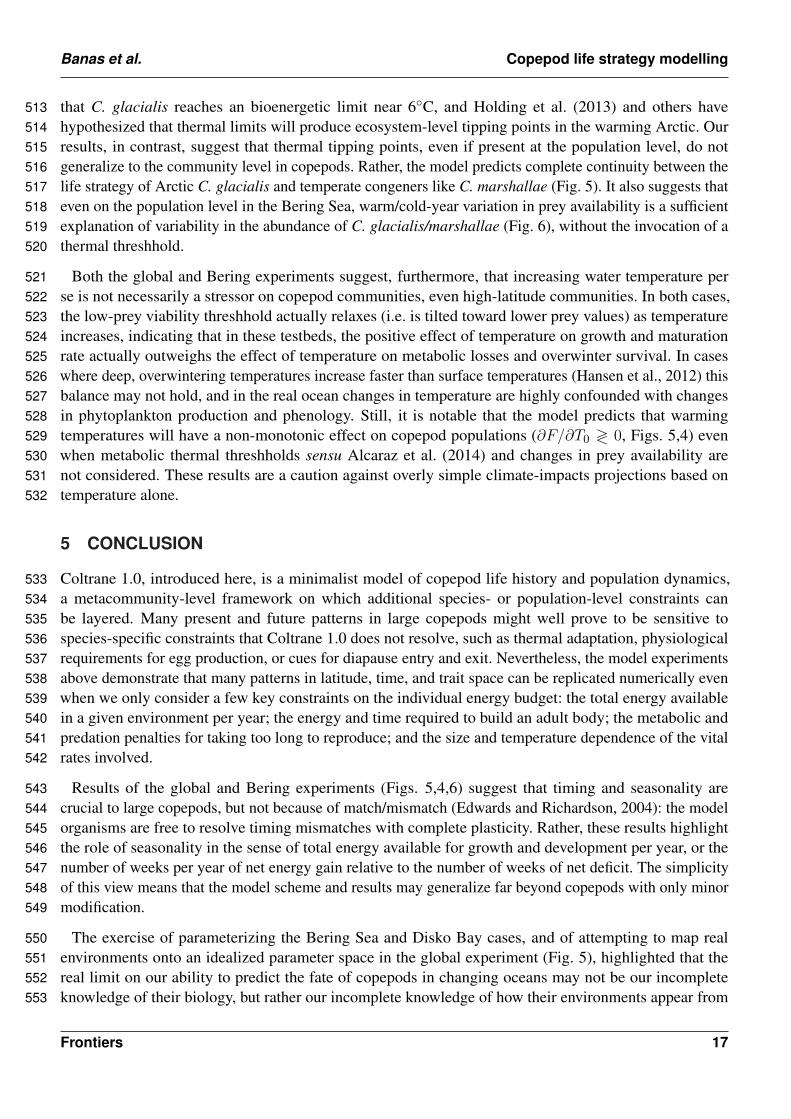
that C. glacialis reaches an bioenergetic limit near 6◦C, and Holding et al. (2013) and others have513hypothesized that thermal limits will produce ecosystem-level tipping points in the warming Arctic. Our514results, in contrast, suggest that thermal tipping points, even if present at the population level, do not515generalize to the community level in copepods. Rather, the model predicts complete continuity between the516life strategy of Arctic C. glacialis and temperate congeners like C. marshallae (Fig. 5). It also suggests that517even on the population level in the Bering Sea, warm/cold-year variation in prey availability is a sufficient518explanation of variability in the abundance of C. glacialis/marshallae (Fig. 6), without the invocation of a519thermal threshhold.520
Both the global and Bering experiments suggest, furthermore, that increasing water temperature per521se is not necessarily a stressor on copepod communities, even high-latitude communities. In both cases,522the low-prey viability threshhold actually relaxes (i.e. is tilted toward lower prey values) as temperature523increases, indicating that in these testbeds, the positive effect of temperature on growth and maturation524rate actually outweighs the effect of temperature on metabolic losses and overwinter survival. In cases525where deep, overwintering temperatures increase faster than surface temperatures (Hansen et al., 2012) this526balance may not hold, and in the real ocean changes in temperature are highly confounded with changes527in phytoplankton production and phenology. Still, it is notable that the model predicts that warming528temperatures will have a non-monotonic effect on copepod populations (∂F/∂T0 ≷ 0, Figs. 5,4) even529when metabolic thermal threshholds sensu Alcaraz et al. (2014) and changes in prey availability are530not considered. These results are a caution against overly simple climate-impacts projections based on531temperature alone.532
5 CONCLUSION
Coltrane 1.0, introduced here, is a minimalist model of copepod life history and population dynamics,533a metacommunity-level framework on which additional species- or population-level constraints can534be layered. Many present and future patterns in large copepods might well prove to be sensitive to535species-specific constraints that Coltrane 1.0 does not resolve, such as thermal adaptation, physiological536requirements for egg production, or cues for diapause entry and exit. Nevertheless, the model experiments537above demonstrate that many patterns in latitude, time, and trait space can be replicated numerically even538when we only consider a few key constraints on the individual energy budget: the total energy available539in a given environment per year; the energy and time required to build an adult body; the metabolic and540predation penalties for taking too long to reproduce; and the size and temperature dependence of the vital541rates involved.542
Results of the global and Bering experiments (Figs. 5,4,6) suggest that timing and seasonality are543crucial to large copepods, but not because of match/mismatch (Edwards and Richardson, 2004): the model544organisms are free to resolve timing mismatches with complete plasticity. Rather, these results highlight545the role of seasonality in the sense of total energy available for growth and development per year, or the546number of weeks per year of net energy gain relative to the number of weeks of net deficit. The simplicity547of this view means that the model scheme and results may generalize far beyond copepods with only minor548modification.549
The exercise of parameterizing the Bering Sea and Disko Bay cases, and of attempting to map real550environments onto an idealized parameter space in the global experiment (Fig. 5), highlighted that the551real limit on our ability to predict the fate of copepods in changing oceans may not be our incomplete552knowledge of their biology, but rather our incomplete knowledge of how their environments appear from553
Frontiers 17
Banas et al. Copepod life strategy modelling
their point of view. How do standard oceanographic measures of chlorophyll and particulate chemistry554relate to prey quality, and how much risk a copepod should take on in order to forage in the euphotic zone?555How do bathymetry, the light field, and other metrics relate to the predator regime? Further experiments556in a simple, fast, mechanistically transparent model like Coltrane may suggest new priorities for field557observations, in addition to new approaches to regional and global modelling.558
APPENDIX: REGIONAL TESTBED FORMULATIONS
Eastern Bering Sea559
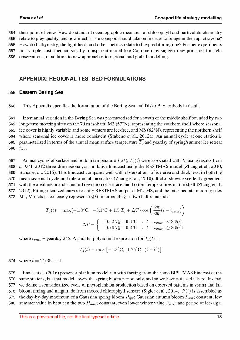
This Appendix specifies the formulation of the Bering Sea and Disko Bay testbeds in detail.560
Interannual variation in the Bering Sea was parameterized for a swath of the middle shelf bounded by two561long-term mooring sites on the 70 m isobath: M2 (57◦N), representing the southern shelf where seasonal562ice cover is highly variable and some winters are ice-free, and M8 (62◦N), representing the northern shelf563where seasonal ice cover is more consistent (Stabeno et al., 2012a). An annual cycle at one station is564parameterized in terms of the annual mean surface temperature T0 and yearday of spring/summer ice retreat565tice.566
Annual cycles of surface and bottom temperature T0(t), Td(t) were associated with T0 using results from567a 1971–2012 three-dimensional, assimilative hindcast using the BESTMAS model (Zhang et al., 2010;568Banas et al., 2016). This hindcast compares well with observations of ice area and thickness, in both the569mean seasonal cycle and interannual anomalies (Zhang et al., 2010). It also shows excellent agreement570with the areal mean and standard deviation of surface and bottom temperatures on the shelf (Zhang et al.,5712012). Fitting idealized curves to daily BESTMAS output at M2, M8, and the intermediate mooring sites572M4, M5 lets us concisely represent T0(t) in terms of T0 as two half-sinusoids:573
T0(t) = max(−1.8◦C, −3.1◦C + 1.5 T0 + ∆T · cos
(2π
365(t− tmax)
)∆T =
{−0.62 T0 + 9.6◦C , |t− tmax| < 365/4
0.76 T0 + 0.2◦C , |t− tmax| ≥ 365/4
where tmax = yearday 245. A parallel polynomial expression for Td(t) is
Td(t) = max[−1.8◦C, 1.75◦C · (t− t5)
]where t = 2t/365− 1.574
Banas et al. (2016) present a plankton model run with forcing from the same BESTMAS hindcast at the575same stations, but that model covers the spring bloom period only, and so we have not used it here. Instead,576we define a semi-idealized cycle of phytoplankton production based on observed patterns in spring and fall577bloom timing and magnitude from moored chlorophyll sensors (Sigler et al., 2014). P (t) is assembled as578the day-by-day maximum of a Gaussian spring bloom Pspr; Gaussian autumn bloom Paut; constant, low579summer value in between the two Psum; constant, even lower winter value Pwin; and period of ice-algal580
This is a provisional file, not the final typeset article 18

Banas et al. Copepod life strategy modelling
availability in late winter/early spring PIA. These are given by581
Pwin = 0.1, taut < t < tspr
PIA = PIA, t ≥ 45 and t < tice + 10
Pspr = Pspr exp(− [(t− tspr)/15]2
)Psum = 1
10 Pspr, tspr < t < taut
Paut =(12 Pspr
)exp
(− [(t− taut)/15]2
)Pspr = 16 mg chl m−3 (Sigler et al., 2014). Prey saturation during the ice algal production period (mid582February until ice retreat: R. Gradinger, pers. comm.) has been assumed to be very high, comparable to583the peak of the spring bloom: PIA = Pspr. This is a gloss over a number of competing considerations. In584reality, in the Eastern Bering Sea, ice algae comprise a much smaller integrated standing stock than the585pelagic bloom (Cooper et al., 2013) and they are likely available to Calanus only intermittently in time.586However, they are extraordinarily concentrated when they are present; they dominate the gut contents of587Calanus during late winter (Durbin and Casas, 2014); and feeding experiments (Campbell et al., 2016)588show that Calanus ingest them at a rate that far exceeds the functional response to pelagic phytoplankton589we have otherwise assumed.590
The date of the autumn bloom maximum taut, which Sigler et al. (2014) show to be relatively invariant,is 265. The date of the spring bloom maximum tspr has the nonlinear relationship with ice-retreat date ticedescribed by the “oscillating control hypothesis” (Hunt et al., 2002):
tspr =
{150 , tice < 75
tice + 10 , tice ≥ 75
Ice-free years are represented by tice = 0.591
Disko Bay592
The Disko Bay testbed was constructed using observations of temperature, phytoplankton, and593microzooplankton from 1996–97 as shown in Fig. 7 (Madsen et al., 2001). For ease of interpretation, we594slightly idealized the forcing time series (instead of interpolating between raw observations) as follows.595
Surface temperature is a piecewise linear function between −0.7◦C on yearday 1, a late-winter minimum596of −1.8◦C on yearday 105, and a summer maximum of 3.7◦C on yearday 250. Deep temperature is set to5971◦C year-round, which matches 1996 observations but omits the arrival of warmer Atlantic deep water in598spring 1997 (Hansen et al., 2012).599
Prey P is assumed to consist of large phytoplankton and microzooplankton. These were summed in600carbon units and then converted to an equivalent chlorophyll concentration using the observed mean601phytoplankton C:chl ratio. Similar to the Bering Sea testbed, it is assembled from the day-by-day maximum602
Frontiers 19

Banas et al. Copepod life strategy modelling
of a Gaussian spring bloom, Gaussian autumn bloom, and constant summer and winter minima:603
Pwin = 0.1, taut < t < tspr
Pspr = Pspr exp(− [(t− tspr)/15]2
)Psum = 1
20 Pspr, tspr < t < taut
Paut =(12 Pspr
)exp
(− [(t− taut)/30]2
)Pspr = 13 mg chl m−3, Pspr = 5 mg chl m−3, tspr = yearday 150, and taut = yearday 225. These timing604parameters are not appropriate for more recent years with less ice cover (e.g., 2008, Fig. 7) but evaluating605the effect of interannual variation on model copepods in Disko Bay, parallel to the Bering Sea experiment606above, is left for future work.607
DISCLOSURE/CONFLICT-OF-INTEREST STATEMENT
The authors declare that the research was conducted in the absence of any commercial or financial608relationships that could be construed as a potential conflict of interest.609
AUTHOR CONTRIBUTIONS
NSB designed the model, performed the analysis, and led the writing of the manuscript. EFM and TGN610helped formulate and interpret the Disko Bay case study, and LBE the Bering Sea case study. All authors611contributed to revision of the manuscript.612
ACKNOWLEDGMENTS
Many thanks to Bob Campbell, Thomas Kiørboe, Øystein Varpe, and Dougie Speirs for discussions that613helped shape both the model and the questions we asked of it.614
Funding: This work was supported by grants PLR-1417365 and PLR-1417224 from the National Science615Foundation.616
REFERENCES
Alcaraz, M., Felipe, J., Grote, U., Arashkevich, E., and Nikishina, A. (2014). Life in a warming ocean:617thermal thresholds and metabolic balance of arctic zooplankton. Journal of Plankton Research 36, 3–10618
Ashjian, C. J., Campbell, R. G., Welch, H. E., Butler, M., and Van Keuren, D. (2003). Annual cycle in619abundance, distribution, and size in relation to hydrography of important copepod species in the western620Arctic Ocean. Deep Sea Research Part I: Oceanographic Research Papers 50, 1235–1261621
Banas, N. S. and Campbell, R. G. (2016). Traits controlling body size in copepods: Separating general622constraints from species-specific strategies. Marine Ecology Progress Series , subm623
Banas, N. S., Zhang, J., Campbell, R. G., Sambrotto, R. N., Lomas, M. W., Sherr, E., et al. (2016).624Spring plankton dynamics in the Eastern Bering Sea, 1971-2050: Mechanisms of interannual variability625diagnosed with a numerical model. Journal of Geophysical Research: Oceans 121, 1476–1501626
Beaugrand, G. and Kirby, R. R. (2010). Climate, plankton and cod. Global Change Biology 16, 1268–1280627
This is a provisional file, not the final typeset article 20

Banas et al. Copepod life strategy modelling
Burke, B. J., Peterson, W., Beckman, B. R., Morgan, C., Daly, E. A., and Litz, M. (2013). Multivariate628Models of Adult Pacific Salmon Returns. PloS one 8, e54134629
Campbell, R. G., Ashjian, C. J., Sherr, E. B., Sherr, B. F., Lomas, M. W., Ross, C., et al. (2016).630Mesozooplankton grazing during spring sea-ice conditions in the eastern Bering Sea. Deep Sea Research631Part II in press632
Campbell, R. G., Wagner, M. M., Teegarden, G. J., Boudreau, C. A., and Durbin, E. G. (2001). Growth633and development rates of the copepod Calanus finmarchicus reared in the laboratory. Marine Ecology634Progress Series 221, 161–183635
Cooper, L. W., Sexson, M. G., Grebmeier, J. M., Gradinger, R., Mordy, C. W., and Lovvorn, J. R. (2013).636Linkages between sea-ice coverage, pelagic-benthic coupling, and the distribution of spectacled eiders:637Observations in March 2008, 2009 and 2010, northern Bering Sea. Deep Sea Research 94, 31–43638
Coyle, K. O., Eisner, L. B., Mueter, F. J., Pinchuk, A. I., Janout, M. A., Cieciel, K. D., et al. (2011). Climate639change in the southeastern Bering Sea: impacts on pollock stocks and implications for the oscillating640control hypothesis. Fisheries Oceanography 20, 139–156641
Daase, M., Falk-Petersen, S., Varpe, Ø., Darnis, G., Søreide, J. E., Wold, A., et al. (2013). Timing of642reproductive events in the marine copepod Calanus glacialis: a pan-Arctic perspective. Canadian Journal643of Fisheries and Aquatic Sciences 70, 871–884644
Durbin, E. G. and Casas, M. C. (2014). Early reproduction by Calanus glacialis in the Northern Bering645Sea: the role of ice algae as revealed by molecular analysis. Journal of Plankton Research 36, 523–541646
Edwards, M. and Richardson, A. J. (2004). Impact of climate change on marine pelagic phenology and647trophic mismatch. Nature 430, 881–884648
Eisner, L. B., Napp, J. M., Mier, K. L., Pinchuk, A. I., and Andrews, A. G. (2014). Climate-mediated649changes in zooplankton community structure for the eastern Bering Sea. Deep Sea Research Part II 109,650157–171651
Ejsmond, M. J., Varpe, Ø., Czarnoleski, M., and Kozłowski, J. (2015). Seasonality in Offspring Value and652Trade-Offs with Growth Explain Capital Breeding. American naturalist 186, E111–E125653
Falk-Petersen, S., Mayzaud, P., Kattner, G., and Sargent, J. R. (2009). Lipids and life strategy of Arctic654Calanus. Marine Biology Research 5, 18–39655
Fiksen, Ø. and Carlotti, F. (1998). A model of optimal life history and diel vertical migration in Calanus656finmarchicus. Sarsia 83, 129–147657
Fiksen, Ø., Utne, A. C. W., Aksnes, D. L., Eiane, K., Helvik, J. V., and Sundby, S. (1998). Modelling658the influence of light, turbulence and ontogeny on ingestion rates in larval cod and herring. Fisheries659Oceanography 7, 355–363660
Follows, M. J., Dutkiewicz, S., Grant, S., and Chisholm, S. W. (2007). Emergent biogeography of microbial661communities in a model ocean. Science 315, 1843–1846662
Forster, J. and Hirst, A. G. (2012). The temperature-size rule emerges from ontogenetic differences between663growth and development rates. Functional Ecology 26, 483–492664
Forster, J., Hirst, A. G., and Woodward, G. (2011). Growth and development rates have different thermal665responses. The American Naturalist 178, 668–678666
Gentleman, W., Leising, A. W., Frost, B. W., Strom, S. L., and Murray, J. (2003). Functional responses for667zooplankton feeding on multiple resources: a review of assumptions and biological dynamics. Deep Sea668Research Part II 50, 2847–2875669
Gurney, W. S. C., Crowley, P. H., and Nisbet, R. M. (1992). Locking life-cycles onto seasons: Circle-map670models of population dynamics and local adaptation. Journal of Mathematical Biology 30, 251–279671
Frontiers 21

Banas et al. Copepod life strategy modelling
Hansen, J., Bjornsen, P. K., and Hansen, B. W. (1997). Zooplankton grazing and growth: Scaling within672the 2-2,000 µm body size range. Limnol Oceanogr 42, 687–704673
Hansen, M. O., Nielsen, T. G., Stedmon, C. A., and Munk, P. (2012). Oceanographic regime shift during6741997 in Disko Bay, Western Greenland. Limnology and Oceanography 57, 634–644675
Hirche, H.-J. and Kattner, G. (1993). Egg production and lipid content of Calanus glacialis in spring:676indication of a food-dependent and food-independent reproductive mode. Marine Biology 117, 615–622677
Hirst, A. G. and Kiørboe, T. (2002). Mortality of marine planktonic copepods: global rates and patterns.678Marine Ecology Progress Series 230, 195–209679
Holding, J. M., Duarte, C. M., and Arrieta, J. M. (2013). Experimentally determined temperature thresholds680for Arctic plankton community metabolism. Biogeosciences 10, 357–370681
Hooff, R. C. and Peterson, W. (2006). Copepod biodiversity as an indicator of changes in ocean and climate682conditions of the northern California current ecosystem. Limnology and Oceanography 51, 2607–2620683
Houston, A. I., McNamara, J. M., and Hutchinson, J. M. C. (1993). General Results concerning the684Trade-Off between Gaining Energy and Avoiding Predation. Philosophical Transactions of the Royal685Society of London. Series B: Biological Sciences 341, 375–397686
Hunt, G. L., Coyle, K. O., Eisner, L. B., Farley, E. V., Heintz, R. A., Mueter, F. J., et al. (2011). Climate687impacts on eastern Bering Sea foodwebs: a synthesis of new data and an assessment of the Oscillating688Control Hypothesis. ICES Journal of Marine Science 68, 1230–1243689
Hunt, G. L., Stabeno, P. J., Walters, G., Sinclair, E., Brodeur, R. D., Napp, J. M., et al. (2002). Climate690change and control of the southeastern Bering Sea pelagic ecosystem. Deep Sea Research 49, 5821–5853691
Kattner, G. and Hagen, W. (2009). Lipids in marine copepods: latitudinal characteristics and perspective to692global warming. In Lipids in Aquatic Ecosystems, ed. M. T. Arts (New York, NY: Springer New York).693257–280694
Kiørboe, T. and Hirst, A. G. (2014). Shifts in Mass Scaling of Respiration, Feeding, and Growth Rates695across Life-Form Transitions in Marine Pelagic Organisms. The American Naturalist 183, E118–E130696
Kiørboe, T. and Sabatini, M. (1995). Scaling of fecundity, growth and development in marine planktonic697copepods. Marine Ecology Progress Series 120, 285–298698
Kleiber, M. (1932). Body size and metabolism. Hilgardia 6, 315–353699
MacDonald, A., Heath, M., Edwards, M., Furness, R., Pinnegar, J., Wanless, S., et al. (2015). Climate--700Driven Trophic Cascades Affecting Seabirds around the British Isles. In Oceanography and Marine701Biology (CRC Press). 55–80702
Madsen, S. D., Hansen, B. W., and Nielsen, T. G. (2001). Annual population development and production703by Calanus finmarchicus, C. glacialis and C. hyperboreus in Disko Bay, western Greenland. Marine704Biology 139, 75–83705
Mantua, N. J., Hare, S. R., Zhang, Y., Wallace, J. M., and Francis, R. C. (1997). A Pacific interdecadal706climate oscillation with impacts on salmon production. Bulletin of the American Meteorological Society70778, 1069–1079708
Maps, F., Pershing, A. J., and Record, N. R. (2012). A generalized approach for simulating growth and709development in diverse marine copepod species. ICES Journal of Marine Science 69, 370–379710
Maps, F., Record, N. R., and Pershing, A. J. (2014). A metabolic approach to dormancy in pelagic711copepods helps explaining inter- and intra-specific variability in life-history strategies. Journal of712Plankton Research 36, 18–30713
McNamara, J. M. and Houston, A. I. (2008). Optimal annual routines: behaviour in the context of714physiology and ecology. Philosophical Transactions of the Royal Society of London. Series B: Biological715Sciences 363, 301–319716
This is a provisional file, not the final typeset article 22

Banas et al. Copepod life strategy modelling
Møller, E. F., Bohr, M., Kjellerup, S., Maar, M., Mohl, M., Swalethorp, R., et al. (????). Calanus717finmarchicus egg production at its northern border . Journal of Plankton Research718
Møller, E. F., Maar, M., Jonasdottir, S. H., Gissel Nielsen, T., and Tonnesson, K. (2012). The effect of719changes in temperature and food on the development of Calanus finmarchicus and Calanus helgolandicus720populations. Limnology and Oceanography 57, 211–220721
Ohman, M. D., Eiane, K., Durbin, E., Runge, J., and Hirche, H.-J. (2004). A comparative study of Calanus722finmarchicus mortality patterns at five localities in the North Atlantic. ICES Journal of Marine Science72361, 687–697724
Ohman, M. D. and Romagnan, J.-B. (2015). Nonlinear effects of body size and optical attenuation on Diel725Vertical Migration by zooplankton. Limnology and Oceanography 61, 765–770726
Olson, M. B., Lessard, E. J., and Wong, C. (2006). Copepod feeding selectivity on microplankton, including727the toxigenic diatoms Pseudo-nitzschia spp., in the coastal Pacific Northwest. Marine Ecology Progress728Series 326, 207–220729
Osterblom, H., Olsson, O., Blenckner, T., and Furness, R. W. (2008). Junk-food in marine ecosystems.730Oikos 117, 967–977731
Peterson, W. T. (1979). Life History and Ecology of Calanus marshallae Frost in the Oregon upwelling732zone. Ph.D. thesis, Oregon State University733
Record, N. R., Pershing, A. J., and Maps, F. (2013). Emergent copepod communities in an adaptive734trait-structured model. Ecological Modelling 260, 11–24735
Runge, J. A., Plourde, S., Joly, P., Niehoff, B., and Durbin, E. (2006). Characteristics of egg production of736the planktonic copepod, Calanus finmarchicus, on Georges Bank: 1994–1999. Deep Sea Research Part737II 53, 2618–2631738
Sainmont, J., Andersen, K. H., Thygesen, U. H., Fiksen, Ø., and Visser, A. W. (2015). An effective739algorithm for approximating adaptive behavior in seasonal environments. Ecological Modelling 311,74020–30741
Saiz, E. and Calbet, A. (2007). Scaling of feeding in marine calanoid copepods. Limnology and742Oceanography 52, 668–675743
Sigler, M. F., Stabeno, P. J., Eisner, L. B., Napp, J. M., and Mueter, F. J. (2014). Spring and fall744phytoplankton blooms in a productive subarctic ecosystem, the eastern Bering Sea, during 1995–2011.745Deep Sea Research Part II 109, 71–83746
Stabeno, P. J., Farley Jr, E. V., Kachel, N. B., Moore, S., Mordy, C. W., Napp, J. M., et al. (2012a). A747comparison of the physics of the northern and southern shelves of the eastern Bering Sea and some748implications for the ecosystem. Deep Sea Research Part II 65-70, 14–30749
Stabeno, P. J., Kachel, N. B., Moore, S., Napp, J. M., Sigler, M. F., Yamaguchi, A., et al. (2012b).750Comparison of warm and cold years on the southeastern Bering Sea shelf and some implications for the751ecosystem. Deep Sea Research Part II 65-70, 31–45752
Swalethorp, R., Kjellerup, S., Dunweber, M., Nielsen, T. G., Møller, E. F., Rysgaard, S., et al. (2011).753Grazing, egg production, and biochemical evidence of differences in the life strategies of Calanus754finmarchicus, C. glacialis and C. hyperboreus in Disko Bay, western Greenland. Marine Ecology755Progress Series 429, 125–144756
Varpe, Ø., Daase, M., and Kristiansen, T. (2015). A fish-eye view on the new Arctic lightscape. ICES757Journal of Marine Science 72, 2532–2538758
Varpe, Ø., Jørgensen, C., Tarling, G. A., and Fiksen, Ø. (2007). Early is better: seasonal egg fitness and759timing of reproduction in a zooplankton life-history model. Oikos 116, 1331–1342760
Frontiers 23

Banas et al. Copepod life strategy modelling
Varpe, Ø., Jørgensen, C., Tarling, G. A., and Fiksen, Ø. (2009). The adaptive value of energy storage and761capital breeding in seasonal environments. Oikos 118, 363–370762
Visser, A. W. and Fiksen, Ø. (2013). Optimal foraging in marine ecosystem models: selectivity, profitability763and switching. Marine Ecology Progress Series 473, 91–101764
Visser, A. W., Mariani, P., and Pigolotti, S. (2008). Swimming in turbulence: zooplankton fitness in terms765of foraging efficiency and predation risk. Journal of Plankton Research 31, 121–133766
Wilson, R. J., Speirs, D. C., and Heath, M. R. (2015). On the surprising lack of differences between767two congeneric calanoid copepod species, Calanus finmarchicus and C. helgolandicus. Progress in768Oceanography 134, 413–431769
Zhang, J., Woodgate, R., and Mangiameli, S. (2012). Towards seasonal prediction of the distribution and770extent of cold bottom waters on the Bering Sea shelf. Deep Sea Research Part II 65-70, 58–71771
Zhang, J., Woodgate, R., and Moritz, R. (2010). Sea Ice Response to Atmospheric and Oceanic Forcing in772the Bering Sea. Journal of Physical Oceanography 40, 1729–1747773
FIGURES
DiskoBay
M2
Newport
ShebaM8
E Be
ring S
ea
45°
60°
75°
180°
Figure 1. Locations of model testbeds. The “global” model experiment spans a gradient fromapproximately Ice Station Sheba to Newport, Oregon and beyond.
This is a provisional file, not the final typeset article 24

Banas et al. Copepod life strategy modelling
0 1 2 3
Fitn
ess
F
0
1
2
3
4
Dev
elop
men
t D
0
0.5
All spawning datesDevelopment completedSustainable pop. growth rate
2 yr cycle
Prey
P
*
1st diapause 2nd diapause1st summer 2nd summer1
Time (yrs)
(a)
(b)
(c)
1 yr cycle
Figure 2. Results of an example model case with u0 = 0.007 d−1, T0 = 1◦C, and δt = 135.
Frontiers 25

Banas et al. Copepod life strategy modelling
Mean surface temperature T0
-2 0 2 4 6 8 10 12 14 16
Adul
t siz
e (µ
g C
)
100
200
1000
20
50
2000
500
model field/lab
structural total
C. glacialis/marshallae
C. finmarchicus/helgolandicus
C. hyperboreus
lab (C. finmarchicus)
lab (C. helgolandicus)
N AtlanticNewport
Bering
Disko Bay
u0 = 0.01 d–1
u0 = 0.007 d–1
u0 = 0.005 d–1
Figure 3. Relationship between adult size Wa and mean temperature T0 in the “global” model experiment,for three values of u0, in comparison with observations and laboratory results. Model results (gray dots)represent structural biomass S, as do observations marked with a ?; observations marked with a ◦ representtotal biomass R + S.
This is a provisional file, not the final typeset article 26

Banas et al. Copepod life strategy modelling
0 100 200 300
0
5
10
15
0 100 200 300
0
5
10
15
0 100 200 300
0
5
10
15
Duration of prey availability ∂t
Annu
al m
ean
surf
ace
tem
pera
ture
(°C
)
(a) (b) (c)
0 1 2 3 4
Maximum egg fitness FRange of viability
2 yr life cycle
1 yr life cycle
u0 = 0.01 d–1 u0 = 0.007 d–1 u0 = 0.005 d–1
Figure 4. Maximum egg fitness (eggs per starting egg per generation) across all combinations oftemperature and duration of prey availability in the “global” experiment. Unfilled contour lines givethe environmental range over which one-year (gray, dotted) and two-year (black, solid) life cycles areviable. The white regions at low prey availability indicate environments in which no timing strategy existsthat allows successful maturation.
0 100 200 300
0
5
10
15
Disko Bay
Newport
Sheba
4+ gen/yr3210.5
Duration of prey availability ∂t
Annu
al m
ean
surf
ace
tem
pera
ture
(°C
)
Figure 5. Generations per year of the optimal strategy in each environmental combination for u0 = 0.007d−1. Ice Station Sheba, Disko Bay, and Newport (Fig. 1) have been placed approximately for comparison.
Frontiers 27

Banas et al. Copepod life strategy modelling
0 20 40 60 80 100 120 140 160 1800
1
2
3
4
5
6
7
8
Prey
sat
urat
ion
0
0.4
0.8
0
0.4
0.8
0
0.4
0.8
Jan 1 Dec 31
Tem
pera
ture
(°C
)
0
5
10
Jan 1 Dec 31
Tem
pera
ture
(°C
)
0
5
10 Surface
Bottom
Annu
al m
ean
surf
ace
tem
pera
ture
(°C
)
Jan 1 Dec 31 Jan 1 Dec 31Jan 1 Dec 31 Jan 1 Dec 31
0
0.5
1
1.5
2
2.5
3
Bloom follows ice retreat
Increasing ice algae
Bloom delayed by winter mixing
Egg
fitne
ss F
Date of ice retreat (yearday)
73234
210 1100
5700 2600
1600
Southeast Bering Sea (M2),1971–2012
Northeast Bering Sea (M8),1971–2012
C. glacialis/marshallae abundance(log mean, ind m–2)
Figure 6. Results of the “Bering” experiment. Color contours give the predicted egg fitness of aC. glacialis/marshallae analog under combinations of ice retreat timing (assumed to control springbloom timing: Appendix) and temperature. Examples of the annual cycles of prey availability P andsurface and bottom temperature T0, Td are given at left and bottom. Dots locate years 1971–2012 in thistiming/temperature parameter space, for the northern (blue) and southern (red) middle shelf. Numbers givethe measured abundance of C. glacialis/marshallae in summer.
This is a provisional file, not the final typeset article 28

Banas et al. Copepod life strategy modelling
Mar Apr May Jun Jul Aug Sep Oct Nov0
5
10
15
20
25
Estim
ated
phy
topl
ankt
on /
ava
ilabl
e pr
ey(m
g ch
l m–3
)
19961997
2008 Total chlChl > 11µmChl > 11µm + microzooplanktonModel
Tem
pera
ture
(°C
)
–2
0
2
4
Mar May Jul Sep NovJan Jan
1996
1997
SurfaceDeep
Figure 7. Observations of temperature and prey in Disko Bay 1996–97 from Madsen et al. (2001) (blueand purple thin lines) used to construct semi-idealized forcing time series for the model (thick grey lines).Three estimates of the prey field are shown, in each case averaged between the surface and subsurfacefluorescence maximum: total chlorophyll (solid), chlorophyll in the >11 µm size fraction (dashed), and>11 µm chlorophyll plus a correction for microzooplankton (dotted). A 2008 phytoplankton time series isshown for comparison (orange), based on integrated phytoplankton carbon scaled to matched the springmaximum in chlorophyll units. Temperature in the upper 50 m (“surface”) and water-column minimumtemperature (“deep”) are also shown.
Frontiers 29

Banas et al. Copepod life strategy modelling
Structural biomass (µg C)
100 1000
Max
imum
fitn
ess
F
0.1
1
10m0 = 0.06
0.07
0.08
0.09
0.06
0.07
0.08
0.09
2 yr life cycle
1 yr life cycle
20050 500
C. finmarchicus C. glacialis C. hyperboreus
Figure 8. Results of the ϕ model for a range of u0 values in the Disko Bay testbed (Fig. 7). Maximum eggfitness F is plotted for one-year and two-year strategies, for each of four values of the mortality scalingparameter m0 (0.06–0.09 d−1), as a function of adult size S. The mean structural weights of the threeCalanus spp. that coexist in Disko Bay are also shown (white triangles, top). Curves of F are shown overranges where survival to adulthood without starvation is possible.
This is a provisional file, not the final typeset article 30
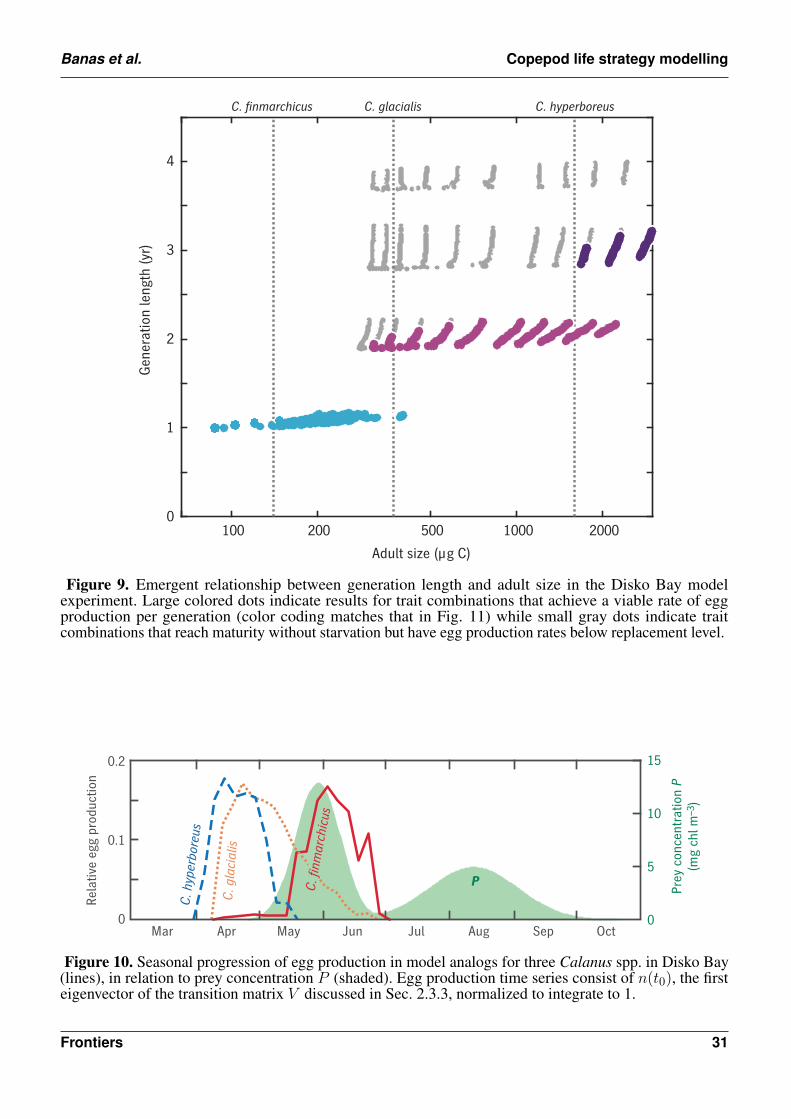
Banas et al. Copepod life strategy modelling
Adult size (µg C)
100 200 500 1000 2000
Gen
erat
ion
leng
th (y
r)
0
1
2
3
4
C. finmarchicus C. glacialis C. hyperboreus
Figure 9. Emergent relationship between generation length and adult size in the Disko Bay modelexperiment. Large colored dots indicate results for trait combinations that achieve a viable rate of eggproduction per generation (color coding matches that in Fig. 11) while small gray dots indicate traitcombinations that reach maturity without starvation but have egg production rates below replacement level.
Prey
con
cent
ratio
n P
(mg
chl m
–3)
Mar Apr May Jun Jul Aug Sep Oct
Rela
tive
egg
prod
uctio
n
C. g
laci
alis
C. h
yper
bore
us
C. fi
nmar
chic
us
0
0.2
0.1
10
5
15
0
P
Figure 10. Seasonal progression of egg production in model analogs for three Calanus spp. in Disko Bay(lines), in relation to prey concentration P (shaded). Egg production time series consist of n(t0), the firsteigenvector of the transition matrix V discussed in Sec. 2.3.3, normalized to integrate to 1.
Frontiers 31

Banas et al. Copepod life strategy modelling
Adult size (µg C) Adult size (µg C)
Adult size (µg C) Adult size (µg C)
50 100 200 500 1000 2000
Med
ian
spaw
ning
dat
e (y
eard
ay)
80
100
120
140
160
180
50 100 200 500 1000 2000
D a
t firs
t dia
paus
e
0.7
0.8
0.9
1
50 100 200 500 1000 2000
Cap
ital f
ract
ion
of e
gg p
rodu
ctio
n
0
0.2
0.4
0.6
0.8
1
50 100 200 500 1000 2000
Mea
n re
serv
e fr
actio
n
0
0.2
0.4
0.6
C4C5
(a) (b)
(c) (d)
Figure 11. Relationships between a number of emergent traits with adult body size in the Disko Bayexperiment. Color coding matches Fig. 9, distinguishing one-year (blue), two-year (light purple) andthree-year (dark purple) life cycles. (a) Median spawning date: compare peaks of egg production curves inFig. 10. (b) Earliest developmental stage D at which diapause (a = 0) occurs: values have been jitteredslightly in the vertical for clarity. (c) Capital fraction of egg production Ecap/(Einc + Ecap). (d) Meanreserve fraction of individual biomass R/(R + S), compared with wax esters as a fration of total bodycarbon for three Calanus spp. from Swalethorp et al. (2011) (open circles).
This is a provisional file, not the final typeset article 32