Embed Size (px)
Citation preview
Author’s Name Name of the Paper Session
DYNAMIC POSITIONING CONFERENCE October 15-16, 2013
RISK SESSION
Cooperative Control Applied to Multi-Vessel DP Operations - Numerical and Experimental Analysis
By Asdrubal N. Queiroz Filho and Eduardo A. Tannuri
University of São Paulo, Numerical Offshore Tank, TPN-USP

Queiroz Filho, A N.; Tannuri, E. A. Risk Session Cooperative Control Applied to Multi-Vessel...
MTS DP Conference - Houston October 15-16, 2013 Page 1
Abstract
Offshore operations involving several floating units are becoming more frequent nowadays. Such
operations are used for sub-sea equipment installation for example. This kind of operations requires a
high level of coordination between the vessels, which today is made without the ship's information
exchange, being each ship individually commanded. Therefore, in those cases, a cooperative control
could be applied, ensuring that the relative distance between the ships are maintained in a limited range,
controlling operational parameters such as the lifting line traction. The benefits of this control are shown
when compared to the non cooperative control by means of an experimental set-up with two DP vessels
and numerical simulations.
Introduction
Nowadays with the increasing of ultra-deep water oil & gas exploration a new concept of "platform" is
rising, where all extracting equipment is placed at the sea's bottom. This new concept is already used in
some fields around the world as in Ormen Lange in Norway (Fig. 1) and has proved to be economically
viable.
Fig. 1. Gas explorations field in Ormen Lange Norway.
Since they are normally large and requires a precise positioning in the sea floor, the installation requires
multi-vessels operations. Those operations require a high level of planning and coordination. An example
that involves the operation of two ships was studied by Fujarra et al. (2008). Multi-vessels operations are
cases where cooperative control could be applied.
Considering the oil & gas industry, there are many other cases where cooperative control could be
applied. In Queiroz et. al. (2012) an oil transfer operation was studied. Two shuttle tankers had to
maintain their relative position while oil was transferred between them, in order to avoid the necessity of
shore terminals. A fully numerical time domain simulation was carried on and the results showed the
benefits of the cooperative control, when compared to the non-cooperative one. In that paper, the
cooperative controller was designed using LQG-LTR control theory applied to the multivariable system
model involving the states of both vessels.
Back to sub-sea equipment installation, it is important to coordinate the relative movement between the
ships in order to properly place the equipment or structure at the sea bottom. This case will be evaluated
in the present paper considering a conceptual experiment.
Queiroz Filho, A N.; Tannuri, E. A. Risk Session Cooperative Control Applied to Multi-Vessel...
MTS DP Conference - Houston October 15-16, 2013 Page 2
The cooperative DP controller will be deeper investigated with the analysis of the coupled dynamics of
the vessels. The influence of the cooperative control gains will be discussed, using the frequency response
and the pole-placement analysis. The consensus control concepts are applied, following Ren et al. (2007).
The advantage of the cooperative control is demonstrated, with the reduction of the relative positioning
error during station keeping or transient manoeuvres.
Fully nonlinear time-domain simulations and a small-scale experiment will be used to demonstrate the
advantages of the cooperative control. All tests are carried out using the TPN's numerical simulator (as
described in Nishimoto et al. 2003) and TPN's physical tank. Two small-scale offshore tugboats models
are used for the scale experiment. Both of them are equipped with two main thrusters at the ship's stern,
two tunnel thrusters, one in the bow and one in the stern.
Mathematical Modeling
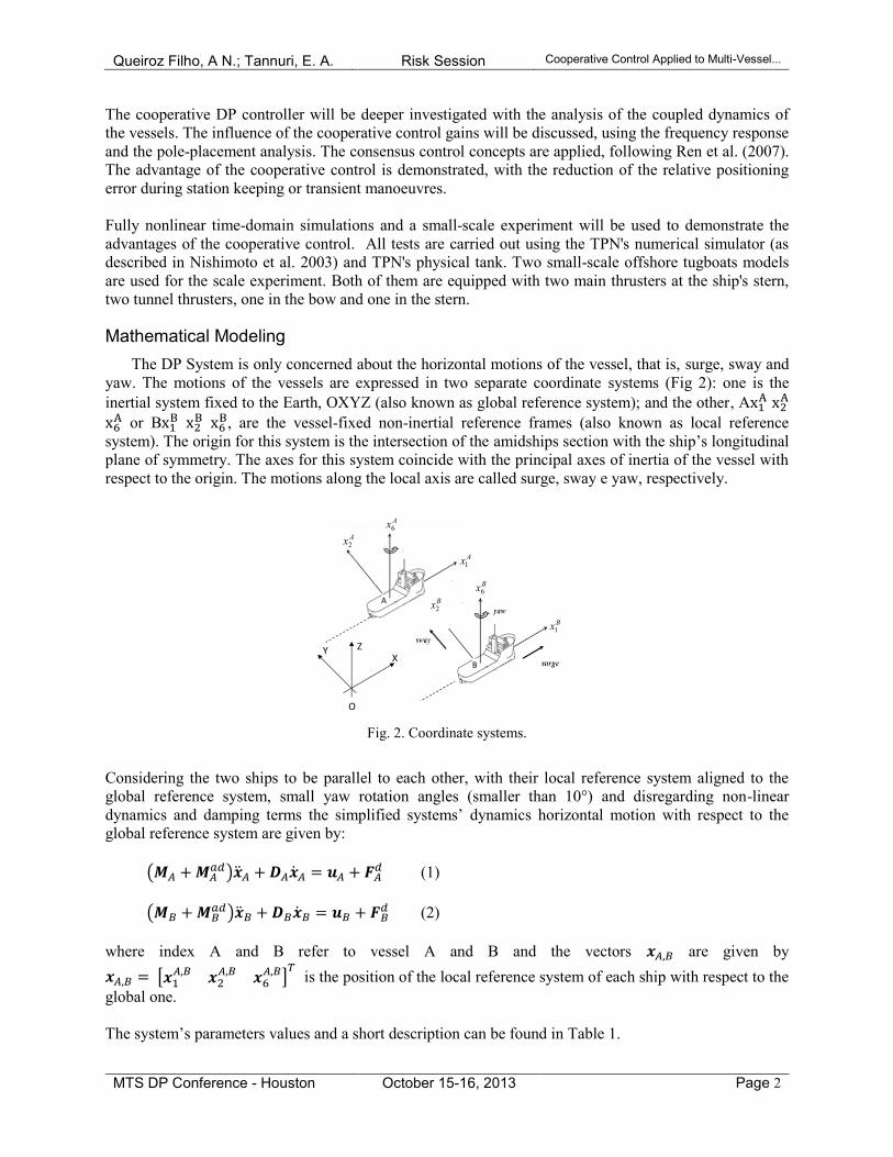
The DP System is only concerned about the horizontal motions of the vessel, that is, surge, sway and
yaw. The motions of the vessels are expressed in two separate coordinate systems (Fig 2): one is the
inertial system fixed to the Earth, OXYZ (also known as global reference system); and the other, A
or B
, are the vessel-fixed non-inertial reference frames (also known as local reference
system). The origin for this system is the intersection of the amidships section with the ship’s longitudinal
plane of symmetry. The axes for this system coincide with the principal axes of inertia of the vessel with
respect to the origin. The motions along the local axis are called surge, sway e yaw, respectively.
Fig. 2. Coordinate systems.
Considering the two ships to be parallel to each other, with their local reference system aligned to the
global reference system, small yaw rotation angles (smaller than 10°) and disregarding non-linear
dynamics and damping terms the simplified systems’ dynamics horizontal motion with respect to the
global reference system are given by:
(1)
(2)
where index A and B refer to vessel A and B and the vectors are given by
is the position of the local reference system of each ship with respect to the
global one.
The system’s parameters values and a short description can be found in Table 1.
Bx1
Ax1
Bx6
Bx2
Ax2
Ax6
B
A
XY Z
O

Queiroz Filho, A N.; Tannuri, E. A. Risk Session Cooperative Control Applied to Multi-Vessel...
MTS DP Conference - Houston October 15-16, 2013 Page 3
Table 1. System’s parameters description.
Parameter Description
Vessel's horizontal displacement matrix
Vessel's added mass matrix
Vessel's linear damping matrix
Vessel's horizontal DP force vector
Vessel's horizontal disturbance force caused by environmental agents
The dynamics of the relative motion can be obtained by eqs. (1) - (2):
(3)
Defining the relative position as and
as the difference of disturbance
forces action on the vessels, the dynamics of the relative motion can be obtained as follows:
(4)
If the two ships are considered to have the same parameters (
, eq. (4) can be simplified as:
(5)
The non cooperative control model
The non cooperative control model is given by 3-uncoupled PID controllers for each vessel. Fig. 3 shows
the control layout.
Fig. 3. Non cooperative control system.
Considering that the two vessels are similar, the same control gains are used. The control law are
then given by:
(6)
Vessel AHorizontal PositionHeading
DP AThrusts
MeasuringSystems +
Filter
Vessel ASet-Point
Calculation
Error+
-
Vessel BHorizontal PositionHeading
DP BThrusts
MeasuringSystems +
Filter
Vessel B Set-Point
Calculation
Error+
-
Desired relativeposition
between the
vessels

Queiroz Filho, A N.; Tannuri, E. A. Risk Session Cooperative Control Applied to Multi-Vessel...
MTS DP Conference - Houston October 15-16, 2013 Page 4
where refers to the position error signal (error in Fig. 3). The , and refers to the PID's
proportional, derivative and integrative diagonal gains matrixes respectively. Replacing eq. (6) in eq. (5)
the non cooperative closed-loop system stays as:
(7)
where is the desired relative position between the vessels (relative position set-point).
The cooperative control model
The cooperative control model combines the existent DP system of each vessel with the consensus
concepts, presented by Ren et al. (2007). In this paper, only a "proportional" consensus gain will be
adopted. Fig. 4 shows the controller layout.
Again the same control law u will be applied to each vessel. For the cooperative control the u control law
is given by:
(8)
where Kc stands for the cooperative "proportional" control gain and
.
Fig. 4. Cooperative control system.
By replacing eq. (8) in eq. (5) the cooperative closed-loop system stays as:
(9)
Vessel AHorizontal PositionHeading
DP AThrusts
MeasuringSystems +
Filter
Vessel ASet-Point
Calculation
Error+-
Vessel BHorizontal PositionHeading
DP BThrusts
MeasuringSystems +
Filter
Vessel B Set-Point
Calculation
Error+
-
Desired relativeposition and
heading
Calculation ofrelative position
and headingerror
++
Kc
-
+
Queiroz Filho, A N.; Tannuri, E. A. Risk Session Cooperative Control Applied to Multi-Vessel...
MTS DP Conference - Houston October 15-16, 2013 Page 5
Numerical Simulations
All experiments were conducted at the TPN's numerical simulator (more about the TPN's numerical
simulator can be found at Nishimoto et al. 2003). The tests were chosen to validate the controller under
two different situations: one is to verify the performance of the controller under tracking (set-point step
change) and another one was chosen to verify the disturbance rejection of the controller (station keeping).
The experiments used two typical offshore tugboats. Theirs properties are indicated at
Table 2.
Table 2. System’s parameters description.
Parameter Value
Length overall LOA 80.0 m
Length between perp. LPP 69.3 m
Beam 18.00 m
Maximum Draft 6.50 m
Minimum (Lightship) Draft 4.60 m
Maximum Displacement 7,881 ton
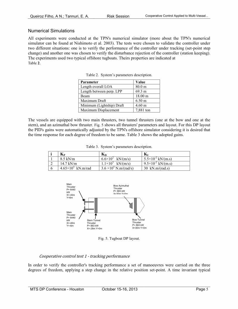
The vessels are equipped with two main thrusters, two tunnel thrusters (one at the bow and one at the
stern), and an azimuthal bow thruster. Fig. 5 shows all thrusters' parameters and layout. For this DP layout
the PID's gains were automatically adjusted by the TPN's offshore simulator considering it is desired that
the time response for each degree of freedom to be same. Table 3 shows the adopted gains.
Table 3. System’s parameters description.
i KP KD KI 1 8.5 kN/m 6.6×10
2 kN/(m/s) 5.5×10
-2 kN/(m.s)
2 14.7 kN/m 1.1×10³ kN/(m/s) 9.5×10
-2 kN/(m.s)
6 4.65×10³ kN.m/rad 3.6 ×10
5 N.m/(rad/s) 30 kN.m/(rad.s)
Fig. 5. Tugboat DP layout.
Cooperative control test 1 - tracking performance
In order to verify the controller's tracking performance a set of manoeuvres were carried on the three
degrees of freedom, applying a step change in the relative position set-point. A time invariant typical
Main Thruster P= 6440 kW X=-40m Y=6m
Main Thruster P= 6440 kW X=-40m Y=-6m
Stern Tunnel Thruster P= 883 kW
X=-28m Y=0m
Bow Tunnel Thruster P= 883 kW
X=30m Y=0m
Bow Azimuthal Thruster P= 883 kW X=30m Y=0m

Queiroz Filho, A N.; Tannuri, E. A. Risk Session Cooperative Control Applied to Multi-Vessel...
MTS DP Conference - Houston October 15-16, 2013 Page 6
Campos Basin environmental condition will be considered during the simulation. Fig 6 shows the
experiment's adopted layout.
Fig. 6. Maneuvers and incoming environmental conditions (Tracking performance evaluation).
Cooperative control test 2 - Disturbance rejection
In order to verify the controller's ability to reject the disturbances, a set of different environmental
conditions will be applied at the system considering a fixed relative distance set-point. At these
simulations, the relative distance set-point will be kept unchanged (30o relative heading angle). At this
experiment the two tugboats were not positioned parallel to each other. In this case, the magnitude of the
disturbances action on the vessels will be significantly different, resulting a large value for the vector .
The wind and wave direction were changed in intervals of 15° around the two vessels, while the current
direction was kept constant. Fig. 7 indicates the experiment layout.
Fig. 7. Incoming environmental conditions (Disturbance rejection evaluation).
Experimental Set-up Description
The experiments were conducted at the Numerical Offshore Tank (USP) (more about the laboratory
facilities for DP experiments can be found at Tannuri et. al 2006 and Morishita et. al. 2009). The tests
were conducted to validate the controller under various environmental conditions. The experiments used
two 1:42 reduced scale model of a typical offshore tugboat, with the full scale properties indicated at
Table 4.
Table 4. Model and Full scale tug boat properties
Property Model
Length overall LOA 1.90 m
Length between perp. LPP 1.65 m
Beam 0.43 m
Maximum Draft 0.154 m
Minimum (Lightship) Draft 0.12m
Maximum Displacement 74 kg
Lightship Displacement 50 kg
X Y
A
B
0.5 m/s Current
4.0m 12s
JONSWAP
Wave
8 m/s wind
50m 30°
15°

Queiroz Filho, A N.; Tannuri, E. A. Risk Session Cooperative Control Applied to Multi-Vessel...
MTS DP Conference - Houston October 15-16, 2013 Page 7
The lightship condition was used in the tests. The two vessels are equipped with two main thrusters, two
tunnel thrusters one in the bow and one in the stern, and an azimuthal thruster which is not going to be
considered in this experiment (Fig. 8).
Fig. 8. Model (upside down) and thrusters information.
The tank has a set of fans and a wave generator that produces wind and waves parallel to the tank (Fig. 9).
A Qualisys measuring system is used for obtaining the horizontal position of both vessels, and the control
loop is performed at the scan rate of 100ms.
Fig. 9. Models under environmental loadings due to fans aligned with the tank length.
For the experimental tests, all PID gains were empirically adjusted, and the Table 5 shows the obtained
values. Both vessel controllers are adjusted with the same gains.
Table 5. KP, KD and KI control gains.
i KP KD KI
1 1.10 N/m 7.57 N.s/m 3.33x10⁻³
N/m.s
2 8.58 N/m 2.08x101 N.s/m 2.00x10
-2 N/m.s
6 1.24x101 Nm/rad 1.52x10
1 N.m.s/rad 1.00x10
-4 Nm/rad.s
X
Y
Z
wind
waves
Main
Thrusters
Tunnel Thrusters
Azimutal
Thruster
(not used)
Queiroz Filho, A N.; Tannuri, E. A. Risk Session Cooperative Control Applied to Multi-Vessel...
MTS DP Conference - Houston October 15-16, 2013 Page 8
Frequency Domain Analysis
Previously to the tests, a frequency domain analysis was performed for both cases: tracking performance
and disturbance rejection.
Tracking performance
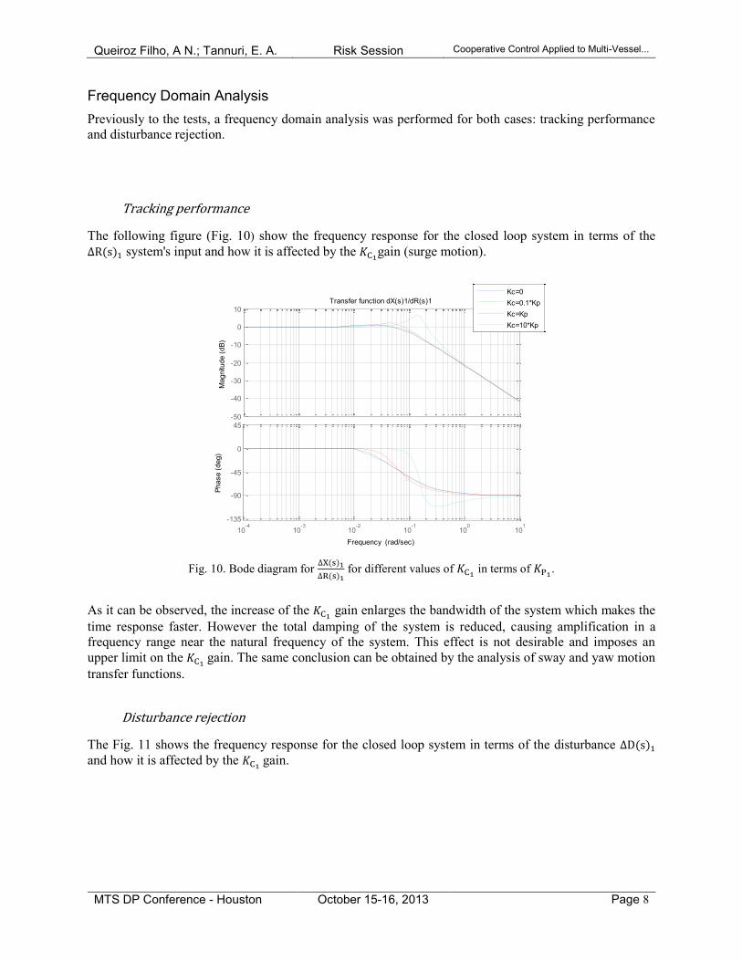
The following figure (Fig. 10) show the frequency response for the closed loop system in terms of the
system's input and how it is affected by the gain (surge motion).
Fig. 10. Bode diagram for
for different values of
in terms of .
As it can be observed, the increase of the gain enlarges the bandwidth of the system which makes the
time response faster. However the total damping of the system is reduced, causing amplification in a
frequency range near the natural frequency of the system. This effect is not desirable and imposes an
upper limit on the gain. The same conclusion can be obtained by the analysis of sway and yaw motion
transfer functions.
Disturbance rejection
The Fig. 11 shows the frequency response for the closed loop system in terms of the disturbance
and how it is affected by the gain.
-50
-40
-30
-20
-10
0
10
Magnitu
de (
dB
)
10-4
10-3
10-2
10-1
100
101
-135
-90
-45
0
45
Phase (
deg)
Transfer function dX(s)1/dR(s)1
Frequency (rad/sec)
Kc=0
Kc=0.1*Kp
Kc=Kp
Kc=10*Kp
Queiroz Filho, A N.; Tannuri, E. A. Risk Session Cooperative Control Applied to Multi-Vessel...
MTS DP Conference - Houston October 15-16, 2013 Page 9
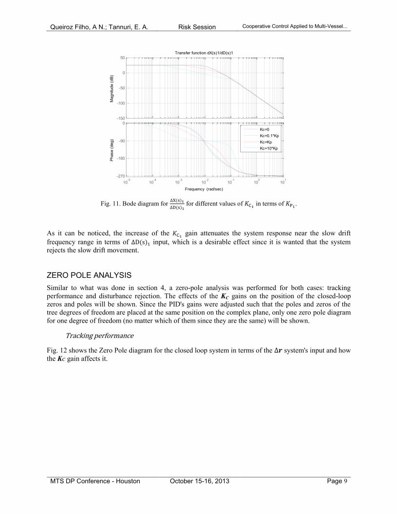
Fig. 11. Bode diagram for
for different values of
in terms of .
As it can be noticed, the increase of the gain attenuates the system response near the slow drift
frequency range in terms of input, which is a desirable effect since it is wanted that the system
rejects the slow drift movement.
ZERO POLE ANALYSIS
Similar to what was done in section 4, a zero-pole analysis was performed for both cases: tracking
performance and disturbance rejection. The effects of the KC gains on the position of the closed-loop
zeros and poles will be shown. Since the PID's gains were adjusted such that the poles and zeros of the
tree degrees of freedom are placed at the same position on the complex plane, only one zero pole diagram
for one degree of freedom (no matter which of them since they are the same) will be shown.
Tracking performance
Fig. 12 shows the Zero Pole diagram for the closed loop system in terms of the system's input and how
the Kc gain affects it.
-150
-100
-50
0
50
Magnitu
de (
dB
)
10-5
10-4
10-3
10-2
10-1
100
101
-270
-180
-90
0
Phase (
deg)
Transfer function dX(s)1/dD(s)1
Frequency (rad/sec)
Kc=0
Kc=0.1*Kp
Kc=Kp
Kc=10*Kp

Queiroz Filho, A N.; Tannuri, E. A. Risk Session Cooperative Control Applied to Multi-Vessel...
MTS DP Conference - Houston October 15-16, 2013 Page 10
(a)
(b)
Fig. 12. Zero pole diagram for
; (a)
; (b)
The increase of the KC gain brings a zero and a first order pole together near the complex axis cancelling
the effect of this pole. The other pair of complex pole, that becomes the dominant one, is removed from
its original position into a farthest position which leaves the system's time response faster. The upper limit
for the KC gain is defined by the damping parameter that defines the overshoot and settling time
parameters.
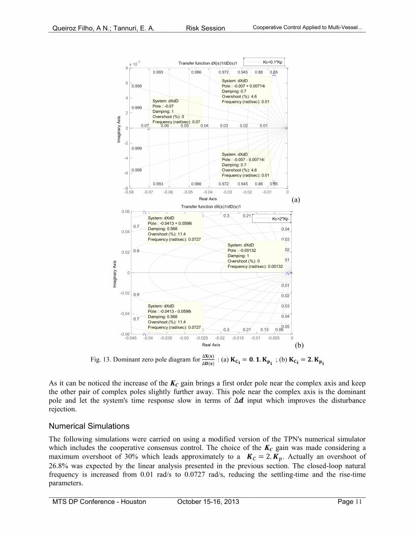
Disturbance rejection
Fig. 13 shows the Zero Pole diagram for the closed loop system in terms of the system's input and how
it is affected by the KC gain.
Transfer function dX(s)1/dR(s)1
Real Axis
Imagin
ary
Axis
-0.04 -0.03 -0.02 -0.01 0 0.01 0.02 0.03
-6
-4
-2
0
2
4
6
8x 10
-3
0.9450.9720.986
0.993
0.998
0.999
0.650.880.9450.9720.986
0.993
0.998
0.999
0.010.020.030.04
System: dXdR
Pole : -0.007 - 0.00714i
Damping: 0.7
Overshoot (%): 4.6
Frequency (rad/sec): 0.01
System: dXdR
Pole : -0.007 + 0.00714i
Damping: 0.7
Overshoot (%): 4.6
Frequency (rad/sec): 0.01
System: dXdR
Zero : -0.00643 + 0.00648i
Damping: 0.704
Overshoot (%): 4.43
Frequency (rad/sec): 0.00913
0.650.88
System: dXdR
Zero : -0.00643 - 0.00648i
Damping: 0.704
Overshoot (%): 4.43
Frequency (rad/sec): 0.00913
Kc=0.1*Kp
Transfer function dX(s)1/dR(s)1
Real Axis
Imagin
ary
Axis
-0.07 -0.06 -0.05 -0.04 -0.03 -0.02 -0.01 0-0.06
-0.04
-0.02
0
0.02
0.04
0.06
System: dXdR
Pole : -0.0413 + 0.0598i
Damping: 0.568
Overshoot (%): 11.4
Frequency (rad/sec): 0.0727
System: dXdR
Pole : -0.0413 - 0.0598i
Damping: 0.568
Overshoot (%): 11.4
Frequency (rad/sec): 0.0727
System: dXdR
Zero : -0.00132
Damping: 1
Overshoot (%): 0
Frequency (rad/sec): 0.00132
System: dXdR
Pole : -0.00132
Damping: 1
Overshoot (%): 0
Frequency (rad/sec): 0.00132
0.10.20.320.440.560.7
0.84
0.95
0.10.20.320.440.560.7
0.84
0.95
0.010.020.030.040.050.060.07
Kc=2*Kp
Queiroz Filho, A N.; Tannuri, E. A. Risk Session Cooperative Control Applied to Multi-Vessel...
MTS DP Conference - Houston October 15-16, 2013 Page 11
(a)
(b)
Fig. 13. Dominant zero pole diagram for
: (a)
; (b)
As it can be noticed the increase of the KC gain brings a first order pole near the complex axis and keep
the other pair of complex poles slightly further away. This pole near the complex axis is the dominant
pole and let the system's time response slow in terms of input which improves the disturbance
rejection.
Numerical Simulations
The following simulations were carried on using a modified version of the TPN's numerical simulator
which includes the cooperative consensus control. The choice of the KC gain was made considering a
maximum overshoot of 30% which leads approximately to a . Actually an overshoot of
26.8% was expected by the linear analysis presented in the previous section. The closed-loop natural
frequency is increased from 0.01 rad/s to 0.0727 rad/s, reducing the settling-time and the rise-time
parameters.
-0.08 -0.07 -0.06 -0.05 -0.04 -0.03 -0.02 -0.01 0-8
-6
-4
-2
0
2
4
6
8x 10
-3
System: dXdD
Pole : -0.07
Damping: 1
Overshoot (%): 0
Frequency (rad/sec): 0.07
System: dXdD
Pole : -0.007 - 0.00714i
Damping: 0.7
Overshoot (%): 4.6
Frequency (rad/sec): 0.01
0.650.880.9450.9720.9860.993
0.998
0.999
0.650.880.9450.9720.9860.993
0.998
0.999
0.010.020.030.040.050.060.070.08
System: dXdD
Pole : -0.007 + 0.00714i
Damping: 0.7
Overshoot (%): 4.6
Frequency (rad/sec): 0.01
Transfer function dX(s)1/dD(s)1
Real Axis
Imagin
ary
Axis
Kc=0.1*Kp
-0.045 -0.04 -0.035 -0.03 -0.025 -0.02 -0.015 -0.01 -0.005 0-0.06
-0.04
-0.02
0
0.02
0.04
0.060.060.130.210.30.40.54
0.7
0.9
0.060.130.210.30.40.54
0.7
0.9
0.01
0.02
0.03
0.04
0.05
0.06
0.01
0.02
0.03
0.04
0.05
0.06
System: dXdD
Pole : -0.0413 + 0.0598i
Damping: 0.568
Overshoot (%): 11.4
Frequency (rad/sec): 0.0727
System: dXdD
Pole : -0.0413 - 0.0598i
Damping: 0.568
Overshoot (%): 11.4
Frequency (rad/sec): 0.0727
System: dXdD
Pole : -0.00132
Damping: 1
Overshoot (%): 0
Frequency (rad/sec): 0.00132
Transfer function dX(s)1/dD(s)1
Real Axis
Imagin
ary
Axis
Kc=2*Kp
Queiroz Filho, A N.; Tannuri, E. A. Risk Session Cooperative Control Applied to Multi-Vessel...
MTS DP Conference - Houston October 15-16, 2013 Page 12
Tracking performance
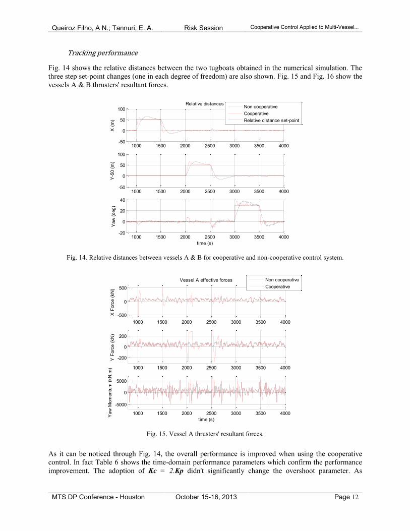
Fig. 14 shows the relative distances between the two tugboats obtained in the numerical simulation. The
three step set-point changes (one in each degree of freedom) are also shown. Fig. 15 and Fig. 16 show the
vessels A & B thrusters' resultant forces.
Fig. 14. Relative distances between vessels A & B for cooperative and non-cooperative control system.
Fig. 15. Vessel A thrusters' resultant forces.
As it can be noticed through Fig. 14, the overall performance is improved when using the cooperative
control. In fact Table 6 shows the time-domain performance parameters which confirm the performance
improvement. The adoption of Kc = 2.Kp didn't significantly change the overshoot parameter. As
1000 1500 2000 2500 3000 3500 4000-50
0
50
100Relative distances
X (
m)
1000 1500 2000 2500 3000 3500 4000-50
0
50
100
Y-5
0 (
m)
1000 1500 2000 2500 3000 3500 4000-20
0
20
40
Yaw
(deg)
time (s)
Non cooperative
Cooperative
Relative distance set-point
1000 1500 2000 2500 3000 3500 4000
-500
0
500
Vessel A effective forces
X F
orc
e (
kN
)
1000 1500 2000 2500 3000 3500 4000
-200
0
200
Y F
orc
e (
kN
)
1000 1500 2000 2500 3000 3500 4000
-5000
0
5000
Yaw
Mom
entu
m (
kN
.m)
time (s)
Non cooperative
Cooperative

Queiroz Filho, A N.; Tannuri, E. A. Risk Session Cooperative Control Applied to Multi-Vessel...
MTS DP Conference - Houston October 15-16, 2013 Page 13
previously stated an overshoot of 26.8% was expected for the cooperative control. Differences in this
parameter for surge and sway can be explained through the disturbance incidence (especially for surge
where the current incidence is aligned to) and thrusters' saturation during the sway manoeuvre (Fig. 15
and Fig. 16). The rise-time and 5% settling-time are significantly improved when comparing to the
standard PID control, showing the benefits of the cooperative control.
Fig. 16. Vessel B thrusters' resultant forces.
Table 6. Cooperative and non-cooperative overshoot comparison.
i Non-cooperative Cooperative
Overshoot
1 27.2% 20.0%
2 28.0% 32.0%
6 27.0% 26.7%
Rise-time
1 67.1s 24.5s
2 70.3s 41.9s
6 55.8s 18.6s
5% settling time
1 440.0s 85.5s
2 450.0s 126.5s
6 435.0s 230.0s
Disturbance rejection
Fig. 17 show the absolute mean relative distance error for each incidence direction considering a 4.0m
significant height and 12s peak period JONSWAP wave, 8m/s wind and 0.5 m/s current.
1000 1500 2000 2500 3000 3500 4000
-500
0
500
Vessel B effective forces
X F
orc
e (
kN
)
1000 1500 2000 2500 3000 3500 4000-400
-200
0
200
400
Y F
orc
e (
kN
)
1000 1500 2000 2500 3000 3500 4000
-5000
0
5000
Yaw
Mom
entu
m (
kN
.m)
time (s)
Non cooperative
Cooperative

Queiroz Filho, A N.; Tannuri, E. A. Risk Session Cooperative Control Applied to Multi-Vessel...
MTS DP Conference - Houston October 15-16, 2013 Page 14
Fig. 17. Absolute mean relative distances for 4.0m significant height and 12s peak period wave, 8 m/s wind and 0.5
m/s current.
As it can be noticed, the overall disturbance rejection is improved when using the cooperative control. In
fact the frequency domain analysis showed a gain reduction near the slow drift frequency range (Fig. 11)
what is also observed in the numerical tests.
Experimental Results
Non-cooperative control
The first experiment was carried out with non-cooperative control. It aims to show that the PID control
gains are well tuned and the performance of the DP positioned vessels is satisfactory for the three degrees
of freedom. No environmental action is considered in this test. Negative and positive steps of 0.2m were
imposed to surge and sway set-points (Fig. 18). The same kind of manoeuvres was imposed to the yaw
angle (10° and 30° step changes).
Fig. 18. Vessel A & B Positions (no environmental action).
0.2
0.4
0.6
0.8
30
210
60
240
90
270
120
300
150
330
180 0
X mean distance error
Non cooperative
Cooperative
0.5
1
1.5
30
210
60
240
90
270
120
300
150
330
180 0
Y mean distance error
Non cooperative
Cooperative
0.5
1
1.5
2
2.5
30
210
60
240
90
270
120
300
150
330
180 0
Yaw mean distance error
Non cooperative
Cooperative
0.2m
10o and30o
X
YB
A
0.2m
Queiroz Filho, A N.; Tannuri, E. A. Risk Session Cooperative Control Applied to Multi-Vessel...
MTS DP Conference - Houston October 15-16, 2013 Page 15
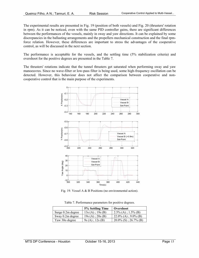
The experimental results are presented in Fig. 19 (position of both vessels) and Fig. 20 (thrusters' rotation
in rpm). As it can be noticed, even with the same PID controller gains, there are significant differences
between the performances of the vessels, mainly in sway and yaw directions. It can be explained by some
discrepancies in the ballasting arrangements and the propellers mechanical construction and the final rpm-
force relation. However, these differences are important to stress the advantages of the cooperative
control, as will be discussed in the next section.
The performance is acceptable for the vessels, and the settling time (5% stabilization criteria) and
overshoot for the positive degrees are presented in the Table 7.
The thrusters' rotations indicate that the tunnel thrusters get saturated when performing sway and yaw
manoeuvres. Since no wave-filter or low-pass filter is being used, some high-frequency oscillation can be
detected. However, this behaviour does not affect the comparison between cooperative and non-
cooperative control that is the main purpose of the experiments.
Fig. 19. Vessel A & B Positions (no environmental action).
Table 7. Performance parameters for positive degrees.
5% Settling Time Overshoot
Surge 0.2m degree 13s (A) ; 19s (B) 2.5% (A) ; 1.5% (B)
Sway 0.2m degree 19s (A) ; 20s (B) 22.0% (A) ; 9.0% (B)
Yaw 30o degree 9s (A) ; 12s (B) 20.0% (S) ; 26.7% (B)
140 160 180 200 220 240 260 280 300-0.4
-0.3
-0.2
-0.1
0
X P
ositio
n(m
)
Vessel A
Vessel B
Set-Point
200 220 240 260 280 300 320-0.9
-0.8
-0.7
-0.6
-0.5
Y P
ositio
n(m
)
Vessel A
Vessel B (+0.9m)
Set-Point
300 320 340 360 380 400 420 440-10
0
10
20
30
40
Time(s)
Yaw
Angle
(deg)
Vessel A
Vessel B
Set-Point

Queiroz Filho, A N.; Tannuri, E. A. Risk Session Cooperative Control Applied to Multi-Vessel...
MTS DP Conference - Houston October 15-16, 2013 Page 16
Fig. 20. Main, Bow and Stern thruster's rotation.
Cooperative control - Test 1 - Yaw manoeuvre, no environmental action
The first set of experiments of the cooperative control consists of 4 maneuvers of 30° step set-point
change in yaw. Fig. 21 illustrates the experiment. No environmental condition is applied in this test, and
the cooperative control gain is varied, in order to illustrate its effects in the overall performance of
the vessels. The cooperative control gains and
are set to zero in this test.
Fig. 21. Maneuvers in yaw.
150 200 250 300 350 400-1000
-500
0
500
1000
Main
Pro
p.
Rota
tion (
rpm
)
Vessel A
Vessel B
150 200 250 300 350 400-4000
-2000
0
2000
4000
Bow
Thru
ste
r R
ota
tion (
rpm
)
Vessel A
Vessel B
150 200 250 300 350 400-4000
-2000
0
2000
4000
Time(s)
Ste
rn T
hru
ste
r R
ota
tion (
rpm
)
Vessel A
Vessel B
X
Y
0.9m 30º
Vessel A
Vessel B

Queiroz Filho, A N.; Tannuri, E. A. Risk Session Cooperative Control Applied to Multi-Vessel...
MTS DP Conference - Houston October 15-16, 2013 Page 17
Fig. 22. Vessel A & B Yaw angle for different cooperative control gain values (no environmental action).
As it can be noticed through Fig. 22 the higher is the gain the closer are the two curves during the
yaw maneuver. It is an indication of the cooperative control working principle. The Fig. 23 presents the
average performance parameters (considering the positive and negative manoeuvres) for the four different
gains. It can be verified that the parameters are getting closer when this gain is 8 or 12.
Fig. 23. Performance parameters.
Another important variable of a multiple vessel operation is the distance between them, considering a
bow, amidships and stern point of the vessels (Fig. 24). In that figure, a dashed line indicates a rough
estimate of the maximum distance variation around the mean value (0.9m). It can be verified the
advantage of the cooperative control, that reduces the distance variation from 0.47m to 0.31m (for
). The cooperative control of the sway motion will reduce this distance variation even more, as
will be shown in the next tests.
40 60 80 100 120 140 160 180 200 220-10
0
10
20
30
40
Yaw
Angle
(deg)
Vessel A
Vessel B
Set-Point
Time (s)
56CxK 8
6CxK0
6CxK 12
6CxK
0%
5%
10%
15%
20%
25%
30%
0 2 4 6 8 10 12
Ove
rsh
oo
t (%
)
Kcx6
0
2
4
6
8
10
12
14
16
0 2 4 6 8 10 12
5%
Se
ttlin
g Ti
me
(s)
Kcx6
Vessel B
Vessel A

Queiroz Filho, A N.; Tannuri, E. A. Risk Session Cooperative Control Applied to Multi-Vessel...
MTS DP Conference - Houston October 15-16, 2013 Page 18
Fig. 24. Distance between different points of the vessels.
The previous results indicated that there was still room to increase the parameter with some
improvement in the performance, without loss of stability. So, after some tests, the Fig. 25 shows the final
comparison for the 30° yaw manoeuvre, with no cooperative control ( ) and with the final value
adopted for yaw cooperative control ( ). Again, the advantages of the cooperative control gets
clear, since the yaw motions of the vessels become quite similar.
Fig. 25. Vessel A & B Yaw angle for two different cooperative control gain values (no environmental action).
Cooperative control - Test 2 - Sway and Yaw manoeuvres, no environmental action
This set of experiments consists of one manoeuvre of 0.2m step set-point change in sway (Fig. 26) with
cooperative control both in yaw and sway axes ( = 12
= 15). Another 5 maneuvers of 30 degrees
step set-point change in yaw were done varying in order to verify the influence of that parameter in
the performance of the controller.
As it can be noticed through Fig. 27 as the gain gets higher the more the both Y position curves get
closer. Fig. 28 shows the absolute relative distance error for the amidships point for the whole test. Fig.
29 shows the relative distance mean error for the same point for every pair of value of (
.
It is evident the benefits of the cooperative control for the sway motion also.
40 60 80 100 120 140 160 180 200 220
0.7
0.8
0.9
1
1.1
Time(s)
Rela
tive D
ista
nce (
m)
Midship
Bow
Stern
Time (s)
06CxK 5
6CxK 8
6CxK 12
6CxK
30 40 50 60 70 80 90 100 110 120-10
0
10
20
30
40
Yaw
Angle
(deg)
Vessel A
Vessel B
Set-Point
06CxK 15
6CxK
Time (s)

Queiroz Filho, A N.; Tannuri, E. A. Risk Session Cooperative Control Applied to Multi-Vessel...
MTS DP Conference - Houston October 15-16, 2013 Page 19
Fig. 26. Maneuvers in sway and yaw.
Fig. 27. Vessel A & B sway position and yaw angle for different cooperative control gain values (no environmental
action).
Fig. 28. Absolute relative distance error for different values of the cooperative control gain (no environmental
action).
50 100 150 200 250 300 350-1
-0.9
-0.8
-0.7
-0.6
Time (s)
Y p
ositio
n (
m)
Vessel A
Vessel B
Set-Point
50 100 150 200 250 300 350
0
20
40
Time (s)
Yaw
Angle
(deg)
50 100 150 200 250 300 3500
0.02
0.04
0.06
0.08
0.1
0.12
0.14
Absolu
te r
ela
tive d
ista
nce e
rror
(m)
Time (s)
X
Y
0.9m
30o
Vessel A
Vessel B
0.2m
Queiroz Filho, A N.; Tannuri, E. A. Risk Session Cooperative Control Applied to Multi-Vessel...
MTS DP Conference - Houston October 15-16, 2013 Page 20
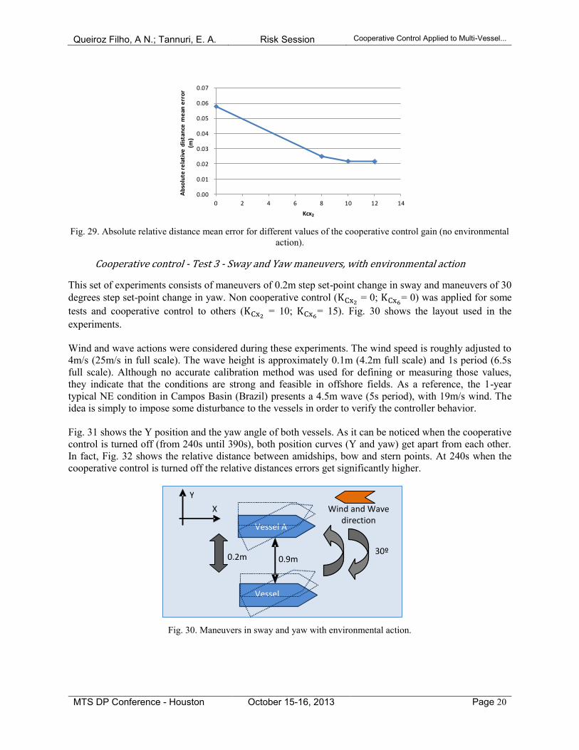
Fig. 29. Absolute relative distance mean error for different values of the cooperative control gain (no environmental
action).
Cooperative control - Test 3 - Sway and Yaw maneuvers, with environmental action
This set of experiments consists of maneuvers of 0.2m step set-point change in sway and maneuvers of 30
degrees step set-point change in yaw. Non cooperative control ( = 0;
= 0) was applied for some
tests and cooperative control to others ( = 10;
= 15). Fig. 30 shows the layout used in the
experiments.
Wind and wave actions were considered during these experiments. The wind speed is roughly adjusted to
4m/s (25m/s in full scale). The wave height is approximately 0.1m (4.2m full scale) and 1s period (6.5s
full scale). Although no accurate calibration method was used for defining or measuring those values,
they indicate that the conditions are strong and feasible in offshore fields. As a reference, the 1-year
typical NE condition in Campos Basin (Brazil) presents a 4.5m wave (5s period), with 19m/s wind. The
idea is simply to impose some disturbance to the vessels in order to verify the controller behavior.
Fig. 31 shows the Y position and the yaw angle of both vessels. As it can be noticed when the cooperative
control is turned off (from 240s until 390s), both position curves (Y and yaw) get apart from each other.
In fact, Fig. 32 shows the relative distance between amidships, bow and stern points. At 240s when the
cooperative control is turned off the relative distances errors get significantly higher.
Fig. 30. Maneuvers in sway and yaw with environmental action.
0.00
0.01
0.02
0.03
0.04
0.05
0.06
0.07
0 2 4 6 8 10 12 14
Ab
solu
te r
ela
tive
dis
tan
ce m
ean
err
or
(m)
Kcx2
X
Y
0.9m
30º
Vessel A
Vessel B
0.2m
Wind and Wave direction

Queiroz Filho, A N.; Tannuri, E. A. Risk Session Cooperative Control Applied to Multi-Vessel...
MTS DP Conference - Houston October 15-16, 2013 Page 21
Fig. 31. Vessel A & B Sway position and Yaw angle with environmental action.
Fig. 32. Relative distance from Keel amidships, bow and stern between the vessels for cooperative and non-
cooperative control.
The amidships relative distance mean error calculated for the cooperative and the non-cooperative control
are respectively 2.41×10⁻²
m and 7.17×10⁻²
m. An improvement of approximately 3 times is verified using
the cooperative control.
Conclusion
This paper presented the application of a cooperative control based on the consensus concept applied
to coordinated manoeuvres. The concept of cooperation control applied to DP operations is innovative
and can be extended to different types of operations that require multiple vessels, such as ship to ship oil
or fuel transfer.
Numerical tests showed that the tracking performance and disturbance rejection of the relative distance
were improved when compared to the standard DP control. The time-domain performance parameters of
150 200 250 300 350 400 450 500 550-1
-0.8
-0.6
-0.4
-0.2
Time (s)
Y p
ositio
n (
m)
Vessel A
Vessel B
Set-Point
150 200 250 300 350 400 450 500 550
0
20
40
Time (s)
Yaw
Angle
(deg)
Cooperative Non-cooperative Cooperative
150 200 250 300 3500.6
0.7
0.8
0.9
1
1.1
Time (s)
Rela
tive d
ista
nce (
m)
Midship
Bow
Stern
Cooperative Non-cooperative

Queiroz Filho, A N.; Tannuri, E. A. Risk Session Cooperative Control Applied to Multi-Vessel...
MTS DP Conference - Houston October 15-16, 2013 Page 22
the system such as the rise-time and settle-time were reduced without significantly changes on the
overshoot parameter. Also the relative distance between the ships varied less when using the cooperative
control. Two tugboats were used in the experiments. Small scale tests also obtained the same results when
using the cooperative control. Two scale model tugboats were used in the experiments.
For a matter of comparison Fig. 33 shows the yaw position for vessels A & B during a 30° yaw step step-
point change for the standard DP control (left) and for the cooperative control (right), for the small scale
experiment. It is observable that the cooperative control approximates both curves.
Fig. 33. Vessels A & B yaw position for non-cooperative control (left) and for the cooperative control (right) during
the small scale experiment.
The same manoeuvre was performed numerically, using the modified TPN simulator and the used
tugboats' models in the tests. Fig. 34 shows the result.
Fig. 34. Vessels' A & B yaw position for non-cooperative control (left) and for the cooperative control (right) during
numerical experiment.
The same behavior is observed on the numerical experiment reinforcing the advantages of the cooperative
control, since the yaw motions of the vessels become quite similar when using the cooperative control. In
other words this is the reduction of the relative distance error provided by the cooperative control.
Acknowledgements
The authors would like to thank the National Council for Scientific and Technological Development
CNPq (process 302544/2010-0), CAPES for the research grant, Brazilian Innovation Agency FINEP
(01.10.0748.00) and São Paulo Research Foundation - FAPESP (2010/15348-4) for sponsoring this
research. The authors also thank Petrobras for the constant support for DP research projects and for the
initial motivation of this work.
30 40 50 60 70 80 90 100 110 120-10
0
10
20
30
40
Yaw
Angle
(deg)
Vessel A
Vessel B
Set-Point
06CxK 15
6CxK
Time (s)
3000 3200 3400 3600 3800 4000-50
0
50Non cooperative control
Yaw
(deg)
time (s)
Vessel A
Vessel B
2800 3000 3200 3400 3600 3800 4000-50
0
50Cooperative control
Yaw
(deg)
time (s)
Vessel A
Vessel B
Queiroz Filho, A N.; Tannuri, E. A. Risk Session Cooperative Control Applied to Multi-Vessel...
MTS DP Conference - Houston October 15-16, 2013 Page 23
References
Fujarra, A. L. C., Tannuri, E. A., Masetti, I. Q., Igreja, H. Experimental and Numerical Evaluation of
the Installation of Sub-Sea Equipments for Risers Support. In: 27th International Conference on
Offshore Mechanics and Arctic Engineering (OMAE2008), Estoril, Portugal, 2008.
Morishita, H.M. ; Tannuri, E. A. ; Saad, A. C. ; Sphaier, S. H. ; Lago, G.A. ; Moratelli JR., L.
Laboratory Facilities for Dynamic Positioning System. In: 8th Conference on Maneuvering and
Control of Marine Craft, MCMC 2009, Guarujá, Brazil, 2009.
Nishimoto, K. et al. (2003). Numerical Offshore Tank: Development of Numerical Offshore Tank for
Ultra Deep Water Oil Production Systems. In: 22nd International Conference on Offshore Mechanics
& Arctic Engineering (OMAE 2003), June, Cancun Mexico 2003.
Queiroz Filho, A. N. ; Tannuri, E. A. ; Da Cruz, J. J., A Shuttle Tanker Position Cooperative Control
Applied to Oil Transfer Operations Based on the LQG/LTR Method. In: 9th Conference on
Maneuvering and Control of Marine Craft. MCMC 2012, Arenzano, Italy, 2012.
Ren, W.; Beard, R.W.; Atkins, E.M., Information Consensus in Multivehicle Cooperative Control,
IEEE Control Systems Magazine, April, 2007.
Tannuri, E.A.; Morishita, H.M. Experimental and Numerical Evaluation of a Typical Dynamic
Positioning System. Applied Ocean Research, v. 28, p. 133-146, 2006.