Cooling of Photovoltaic Cells

Bryce Cruey

Jordan King

Bob Tingleff

December 7, 2006

Contents

List of Figures ii

List of Tables ii

1 Introduction 2

2 Objectives and Constraints 2

3 Literature Review 4

3.1 Concentrated illumination . . . . . . . . . . . . . . . . . . . . . . . . . . . . 4

3.2 Electrical efficiency . . . . . . . . . . . . . . . . . . . . . . . . . . . . . . . . 5

3.3 Hybrid PV/Thermal (PV/T) systems . . . . . . . . . . . . . . . . . . . . . . 6

3.3.1 Duct cooling . . . . . . . . . . . . . . . . . . . . . . . . . . . . . . . . 7

3.3.2 Cooling by the Addition of Fins . . . . . . . . . . . . . . . . . . . . . 9

4 Problem Development 10

5 Model Development 14

5.1 Energy Balance . . . . . . . . . . . . . . . . . . . . . . . . . . . . . . . . . . 14

5.2 Radiation Transmission . . . . . . . . . . . . . . . . . . . . . . . . . . . . . . 15

5.3 Thermal Heat Transfer Coefficient-Natural Convection . . . . . . . . . . . . 16

5.4 Thermal Heat Transfer Coefficient-Forced Convection . . . . . . . . . . . . . 17

5.5 One Dimensional Heat Transfer in a Fin . . . . . . . . . . . . . . . . . . . . 18

i

5.6 Galerkin Finite Element Solution . . . . . . . . . . . . . . . . . . . . . . . . 22

6 Computer Algorithm 26

7 Results and Discussion 27

8 Conclusions 32

Appendix 1 33

A.1.1Analytical Solution Derivation . . . . . . . . . . . . . . . . . . . . . . . . . . 33

ii

List of Tables

1 Table of Nomenclature . . . . . . . . . . . . . . . . . . . . . . . . . . . . . . 1

4.1 model parameters . . . . . . . . . . . . . . . . . . . . . . . . . . . . . . . . . 11

5.1 Finite element basis function descriptions. . . . . . . . . . . . . . . . . . . . 24

List of Figures

2.1 PV panel with fins and duct . . . . . . . . . . . . . . . . . . . . . . . . . . . 3

4.1 PV panel with fins and duct . . . . . . . . . . . . . . . . . . . . . . . . . . . 10

(a) Panel with fins and duct assembly. . . . . . . . . . . . . . . . . . . . . 10

(b) Layers and fin assembly. . . . . . . . . . . . . . . . . . . . . . . . . . . 10

4.2 Equivalent thermal circuit to the system described in Figure 4.1. . . . . . . . 12

5.1 Nodal breakdown of the fin shown in Figure 4.1. Elements in the region are

described by e1 · · · en and nodal points are described by n1 · · ·nn . . . . . . . 24

6.2 Computer flow diagram detailing the progression of events for the solution to

the heat transfer in the PV system. . . . . . . . . . . . . . . . . . . . . . . . 26

7.1 Effect of Single Parameter Change on Panel Efficiency and Cell Temperature 28

(a) Cooling Fluid Velocity . . . . . . . . . . . . . . . . . . . . . . . . . . . 28

(b) Fin Thickness . . . . . . . . . . . . . . . . . . . . . . . . . . . . . . . 28

(c) Fin Spacing . . . . . . . . . . . . . . . . . . . . . . . . . . . . . . . . 28

(d) Fin Length . . . . . . . . . . . . . . . . . . . . . . . . . . . . . . . . . 28

7.2 Effect of Single Parameter Change on Panel Power and q Duct . . . . . . . . 30

iii

(a) Cooling Fluid Velocity . . . . . . . . . . . . . . . . . . . . . . . . . . . 30

(b) Fin Thickness . . . . . . . . . . . . . . . . . . . . . . . . . . . . . . . 30

(c) Fin Spacing . . . . . . . . . . . . . . . . . . . . . . . . . . . . . . . . 30

(d) Fin Length . . . . . . . . . . . . . . . . . . . . . . . . . . . . . . . . . 30

7.3 Effect of Solar Concentration on Panel Operation . . . . . . . . . . . . . . . 31

(a) Panel Efficiency and Cell Temperature . . . . . . . . . . . . . . . . . . 31

(b) Panel Power and q Duct . . . . . . . . . . . . . . . . . . . . . . . . . . 31

7.4 Effect of Fin Material Conductivity on Panel Operation . . . . . . . . . . . . 32

iv

Abstract

The cooling of a photovoltaic panel via fins and a duct attached to the rear surface of the

panel is investigated. Forced convection through the duct is assumed. A model is developed

which allows study of the effects of varying fin parameters on panel electrical output and

potential useful heat output. Electrical output is found to vary weakly with fin material and

thickness, and strongly with fin length and air velocity in the duct. The model suggests a

maximum value of solar concentration for a given air velocity in the duct.

Nomenclature

Table 1: Table of Nomenclature

Symbol Description Unitsqconvf convective heat flux through front of panel (W/m2)qradf radiative heat flux through front of panel (W/m2)qcg heat flux through glass and front half of PV cell (W/m2)qcs heat flux through back half of PV cell to rear surface of panel (W/m2)qfin heat flux through fin (W/m2)qradb radiative heat flux through rear surface of panel (W/m2)qconvb convective heat flux through rear surface of panel (W/m2)h̄ average convective heat transfer coefficient (W/m2 · K)Tg glass surface temperature (K)Tc PV cell temperature (K)Ts panel rear surface temperature (K)Tef front environment temperature (K)Teb back environment temperature (K)Tr surface opposite to rear panel surface temperature (K)σ Stefan-Boltzman constant (5.67 × 10−8W/m2K−4)vw wind velocity (m/s)k thermal conductivity (W/m2K)Rgc thermal resistance from glass through top half of cell (m2K/W )Rcs thermal resistance from midpoint of cell through substrate (m2K/W )ε surface emissivity unitlessLfin fin height (m)tfin fin thickness (m)wfin fin length (m)∆Sf fin spacing (m)A area of panel (m2)I, I2 solar irradiance (W/m2)Pe electrical power (W/m2)Nu Nusselt Number NonePr Prandtl Number NoneRa Rayleigh Number NoneGr Grashof Number Noneβ 1/T K−1

ν Kinematic Viscosity m2/sα Adsorptivity of the surface material NoneRe Reynolds Number None

1

1 Introduction

The cooling of photovoltaic (PV) cells is a problem of great practical significance. The usable

energy produced from solar energy displaces energy produced from fossil fuels, and thereby

contributes to reducing global warming. However, the high cost of solar cells is an obstacle

to expansion of their use.

PV cooling has the potential to reduce the cost of solar energy in three ways. First, the

electrical efficency of PV cells decreases with temperature increase. Cooling can improve the

electrical production of standard flat panel PV modules. Second, cooling makes possible the

use of concentrating PV systems. Cooling keeps the PV cells from reaching temperatures at

which irreversible damage occurs, even under the irradiance of multiple suns. This makes

it possible to replace PV cells with potentially less expensive concentrators. Finally, the

heat removed by the PV cooling system can be used for building heating or cooling, or in

industrial applications.

2 Objectives and Constraints

The objective here is to investigate a technologically straightforward means of cooling a

standard PV panel. The constraints specified at the outset were that the technology be

relatively inexpensive, that it would involve modifications to a standard PV panel, that

useful heat could be recovered, and that it would allow for low level concentration factors

(less than 5X). The goal is to develop a model that allows a sensitivity analysis of basic

parameters. A specific design is not derived, as cost parameters were not investigated.

The method of cooling investigated is fins attached to the rear face of the panel. The rear

surface of the panel is a substrate such as aluminum or copper. The fins are modeled as

being an extension of this substrate. The substrate material is soldered or attached with

adhesive to the rear surface of the cells. Values for thermal conductivity are taken from the

2

literature. In addition, a rectangular duct is attached to the rear surface of the panel, as

shown in Figure 2.1. The duct allows air to be blown across the rear surface of the panel

and potentially captured and used.

Lp

Duct

} wp

Lf

tf tf

wf

tg ta tc tso ts

g a c so s

Fig. 2.1: PV panel with fins and duct

Parameters of the system that are varied are fin thickness, fin height, fin material, air velocity,

and solar concentration. Outputs of the model are cell temperature, cell efficiency, electrical

output, and energy leaving the system through the duct. Constants of the system are panel

element thicknesses and conductivities, and the ambient temperature.

3

3 Literature Review

3.1 Concentrated illumination

Royne et al. (2005), in a review of PV cooling methodologies, for use under concentrated

illumination, provide a set of requirements for cooling techniques. The cooling method needs

to ensure that the operating temperature does not exceed the point at which irreversible

degradation occurs in the cell. In addition, it is desirable for the temperature to be uniform

across the cells, for the technology to be reliable and simple, for the thermal energy produced

to be useable, for the pumping power to be minimal, and for the cooling technology to be

efficient in the use of materials. The authors note that there is an inherent conflict in

the desire to keep the temperature low to enhance electrical efficiency, and to have a high

temperature, thereby increasing the usefulness of the thermal energy.

These authors define three basic geometries of concentrated PV systems: 1. Single-cell point

focus; 2. A linear row of cells; 3. Densely packed cells. Royne et al. (2005) found that for

a single cell geometry, passive cooling with natural convection could theoretically be used

at concentrations up to 1000×, with a cell diameter around 5mm. In a linear arrangement,

passive cooling could be used for concentrations of 10 or 20 suns. Heat pipes can also be used

in this configuration. At higher concentrations forced convection with air or water is required,

with air circulation becoming too costly at higher concentrations, and water preferred. In

densely packed configurations, active cooling is required. Micro-channels etched in the silicon

for water transport can reportedly maintain a temperature of 40◦C under an irradiance of

500 kW/m2. Other techniques include impinging jets, submerging the cells in liquid, boiling

the coolant, and coolant channels in thermal contact with the cells.

Depending on the application, the average heat transfer coefficient can be used (the ratio of

the rate of heat removal to average temperature difference), or it may be necessary to use

local heat transfer coefficients (Royne et al., 2005). An average coefficient can be taken from

the literature, or it may be necessary to model its variation with temperature.

4

In their review, Royne et al. (2005) found that it was common to model heat transfer through

the panel as a series of thermal resistances, with separate resistance values for cover glass,

adhesive, PV cell, solder, and substrate. A linearized version of the heat transfer due to

radiation is used, in which the flux varies with the fourth power of the ambient temperature,

and the first power of the surface temperature.

Sala (1989) presents a theoretical overview of cooling PV cells under concentration in con-

ditions of still air at 25◦C. He finds that, without concentration, if a cell can radiate from

both faces, radiation alone is sufficient to cool the cell. He also finds that natural convection

alone would lead to a temperature increase of 72.5◦C with no concentration, and an increase

of 974◦C with 10× concentration. Forced convection with air as the coolant could limit the

theoretical temperature increase to 282◦C at 10× concentration. If water cooling is used,

temperature increases of 18◦C at 100×, and 189◦C at 1000×, are possible with the flow fully

turbulent. Sala further finds that, considering either radiation or convection alone, if the

radiation (or dissipating) surface area is twice the size of the cell area times the effective

concentration, concentrations of 200× are possible while maintaining temperatures within

the range in which the electrical efficiency is equal to or better than the reference efficiency.

When radiation and convection are combined, Sala finds that with stagnant air, and ignor-

ing albedo radation, radiative losses account for up to 60% of the heat removal. With wind

speed of 2m/s the losses from radation can be 30% of the total.

3.2 Electrical efficiency

A typical value for PV efficiency loss with temperature is 0.5%/◦C (SEI, 2004), though this

varies with the type of cell. Sala (1989) notes that the rate of reduction with temperature

decreases with concentration. Tripanagnostopoulos et al. (2001) argue that, in a standard

PV module, the improvements in electrical efficiency alone cannot justify the costs of the

cooling system, and that cooling is only cost effective if concentration is used, or if the energy

recovered through cooling is put to use.

5

Krauter (2004) investigated a method of reducing reflection which also provided cooling -

replacing the front glass surface with a thin (1mm) film of water running over the face of the

panel. He notes that the refractive index (1.3) of water is superior to that of glass. Reflective

losses in glass can lead to losses in yield of 8-15%. The water decreased cell temperatures

up to 22◦C. The improved optics and cell temperatures increased electrical yield 10.3% over

the day (8-9% after accounting for pumping energy). He also noted an unexpected aesthetic

benefit.

Meneses-Rodriguez et al. (2005) considered a novel technique to improve the electrical ef-

ficiency with cooling. The authors explored the benefits of running PV cells at near their

maximum theoretical temperatures (100-170◦C). Theoretically, the electrical efficiency can

be in the range 10-16%. The cooling fluid would be used to run a Stirling engine. With

a sink temperature of 30◦C, the authors estimate a theoretical total efficiency greater than

30%.

3.3 Hybrid PV/Thermal (PV/T) systems

Vokas et al. (2005) investigated PV/T systems. They studied the thermal energy benefits

of a thermal collector with a PV laminate attached to the front. They found the theoretical

efficiency of the system was 9% lower than that of conventional thermal collectors. They

estimate that a 30m2 collector of this type would provide 54% of the heating and 32% of the

cooling of a typical house in Athens.

Tripanagnostopoulos et al. (2001) also investigated hybrid PV/Thermal (PV/T) systems. In

a PV/T system, the thermal energy is put to use – typically for space heating, water pre-

heating, ventilation, or for industrial applications such as food drying. They experimented

with water cooling, with channels attached to the rear surface of the PV module, with an air

cooling duct, and with additional glazing on the front surface of the PV module to increase

heat retention. They note that the contact between the copper sheet and pipes is a crucial

aspect of the design. Thermal efficiency is calculated as the ratio of the heat carried away

by the convecting fluid to the input insolation. In addition, flat, diffuse reflectors were

6

used to concentrate additional illumination onto the panel, yielding a concentration factor

of up to 1.5. They found that while the glazing increased the thermal efficiency up to 30%,

there were 16% losses in electrical efficiency due to optical effects. The reflectors, at 1.3×,

increased electrical output by 16%. The water was more effective at removing heat than the

air, achieving thermal efficiencies of 71%, compared with 59% for the air coolant. They note

that the enhanced electrical efficiency (up to 3.2%) is not cost-effective unless the thermal

energy is also used.

The thermal efficiency equations of Duffie and Beckman (1991) for solar collectors can be

used to evaluate the thermal performance of a PV panel. These authors derive the useful

energy gain of a collector as a linear relationship of the temperature difference between inlet

fluid temperature and ambient temperature, and a collector heat removal factor.

Another well-known technique for thermal analysis of flat plate solar collectors is the Hottel-

Whillier (HW) method. Duffie and Beckman (1991) set forth the general assumptions of

the model and describe its usefulness in terms of relevant energy coefficients calculated from

simplified mathematics. The model depicts convection, conduction, and radiation as resis-

tive elements combined in series and parallel to form the overall heat loss coefficients for

a solar collector. The pertinent equations are based on the temperature gradient between

parallel plates, thermal conductivities, emissivities, and collector plate dimensions. The use

of the Hottel-Whillier model is substantiated for conventional collector design by de Winter

(1990). The model is extended by Florschuetz (1976)to the analysis of a combined photo-

voltaic/thermal collector system. This extension preserves the general form of the HW model

by modifying existing model parameters to incorporate electrical output. The modifications

of the original equations are based on the assumption that cell efficiency decreases linearly

with increasing local temperature.

3.3.1 Duct cooling

In addition to the study cited above, a number of other authors investigated cooling of a

flat panel PV module with a duct thermally attached to the rear face of the module. Forced

7

or natural convection can be used. Fins and other additional elements can be used within

the duct. This method can be incorporated into building-integrated PV, with an air space

behind the PV module, and the heat captured and put to use within the building (Figure

2.1).

Brinkworth and Sandberg (2006) analyzed cooling of a PV module via a duct attached to its

rear face. Natural convection through the duct removed heat from both the back face of the

PV panel, and the opposite face, which warms through radiation from the back face. They

found that, with an irradiance of 200W/m2, the duct reduced the temperature rise in the

module by 11◦C in still air, and 14◦C in air moving at 2 m/s. The authors combined Newton’s

law of cooling, the experimentally determined proportion of 60% of the heat removed at the

top of the duct by convection (40% by radiation), reported values for the Nusselt number,

and an energy balance at the top opening of the duct. For Reynolds numbers from 7000

to 20,000, they found that the optimum length to hydraulic depth ratio should range from

22 to 17. In another study (Brinkworth, 2006), the authors both experimentally and with

computer modelling of the heat transfer and fluid mechanics found the optimum length to

hydraulic depth ratio for the duct was around 20. They also found that netting across the

ends, and the presence of structural members inside the ducts, had a net positive effect by

increasing the turbulence, even at the expense of reduced air speed.

Tonui and Tripanagnostopoulos (2006) also investigated the use of an air duct attached to

the rear face of a panel. They analyzed two possible improvements to the basic duct: the

addition of a thin metal sheet parallel to the surface of the PV panel in the middle of the

duct, and the addition of fins along the rear surface of the duct. Experimental results showed

thermal efficiencies of 30% with fins, 28% with the thin metal sheet, and 25% with the basic

duct. In the enhanced ducts, the increased convection losses from the additional surfaces

lower the temperatures of those surfaces, thereby increasing radiation losses from the PV

back face. The thin metal sheet has the additional benefit of reducing the temperature of the

back wall of the duct (which is presumably in contact with a building surface). They note

8

that the pumping power to force air through the duct may be achieved with the improved

electrical efficiency provided by the cooling.

3.3.2 Cooling by the Addition of Fins

Effective heat transfer through fins has been well documented (White (1984), Segerland

(1984), Chapman (1984)). The basic theory is to include a fin attachment at the base of

a structure in order to increase its surface area and thereby increase the heat flux (White,

1984). The equation are those that account for both conductive and convective heat transfer

and can be modeled by the convection dispersion equation in space and time (Segerland,

1984). However in an ideal solution as shown by White (1984) and many others, heat

transfer through a fin can be simplified to one dimension and steady state. In this ideal

case where the temperature varies in one direction, the base temperature of the fin is the

temperature at the attachment or junction with what it is that is being cooled (White, 1984).

This generalized approach is a good first approximation of the temperature gradient in the

fin.

The convection-dispersion equation has been well studied and has been solved analytically

in one dimension for a variety of different conditions (W.J. and van Genuchten, 1982). The

convection-dispersion has also been solved numerically using a variety of different methods

including finite elements, finite difference, quasilinearization, and probabalistic/statistical

methods (Willis and Yeh (1987), Segerland (1984)).

Fins are constructed with high thermal-conductivity metals (copper, aluminum, etc.). They

should be designed so that they are more than 60% efficient (White, 1984). Sizing the fins

can be done optimally in cases when the total volume of the fin is held constant and only

one of the physical dimensions are varied. This optimal sizing is based on maximizing the

total heat transfer through the fin while holding the volume constant and changing one of

the physical dimensions of the fin (Began Adrian, 1996). With that in mind cooling PV

panels using fins may be an economical choice.

9

4 Problem Development

The method of PV module cooling investigated here is direct attachment of fins to the rear

surface of the panel. The physical system is described by the layers making up the PV array

and the attached fin on the back as seen in Figure 1(b). A duct is added for which the heat

transfer parameters are based on the assumption of forced convection (1(a)). It is important

to clearly define boundary conditions before this analysis can be executed. The input to

the system is the solar irradiance (I in Figure 1(a)). The boundary conditions are the heat

losses due to radiation and convection on the front and back (qradn , qconvn), as well as the

electrical power output (Pe in Figure 1(b)).

Average heat transfer coefficients for the front and rear surfaces are calculated based on

standard equations. Various values of concentration are modeled, in order to predict the

extent of cooling required under multiple suns.

∆Sf

Lp

Duct

} wp

I

(a) Panel with fins and duct assembly.

Lf

tf tf

wf

tg ta tc tso ts

Tg Tc Ts

Tf

g a c so s

qradf

qconvf

qradb

qconvb

qfin

(b) Layers and fin assembly.

Fig. 4.1: PV panel with fins and duct

10

The model used here extends the approach of Royne et al. (2005). The PV panel is conceived

as consisting of the layers shown in Figure 4.1. The layers in Figure 4.1 are described as

follows:

g = Cover glass layer with thickness tg

a = Adhesive layer with thickness ta

c = Cell layer with thickness tc

c = Solder layer with thickness tso

s = Substrate layer with thickness ts

The fins are an extension of the substrate layer that is attached to the rear surface of the

panel.

The PVCOOL model was developed to model the physical situation. The physical schematic

described in Figure 4.1 (a), and (b) as it applies to our problem uses default parameters in the

PVCOOL model. The thermodynamic properties of the panel, thermodynamic properties of

the fin , and physical dimensions of the panel layers were held constant during throughout

the experiment unless otherwise specified by the user. Default parameter values were taken

from Royne et al. (2005) and are listed in Table 4.1.

Table 4.1: model parametersParameter Value Units Parameter Value UnitsTef

298 K Lfin 0.2 m

kg 1.4 W/m·K tf 0.02 mkc 145 W/m·K ts 1 × 10−4 mks 50 W/m·K tg 3 × 10−3 mkfin 120 W/m·K tc 12×10−5 mka 145 W/m·K ta 1×10−4 mεf 0.855 tsub 2×1−3 mεb 0.8 I 1113 W/m2

Lp 1 m ρ 0.05wf 1 m U∞ 2 m/swp 1 m θ 46.336∆Sf 0.2 m

11

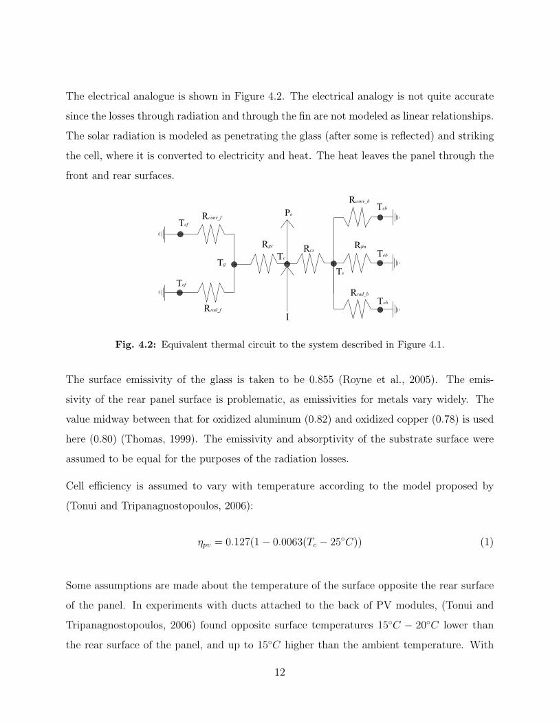
The electrical analogue is shown in Figure 4.2. The electrical analogy is not quite accurate

since the losses through radiation and through the fin are not modeled as linear relationships.

The solar radiation is modeled as penetrating the glass (after some is reflected) and striking

the cell, where it is converted to electricity and heat. The heat leaves the panel through the

front and rear surfaces.

Fig. 4.2: Equivalent thermal circuit to the system described in Figure 4.1.

The surface emissivity of the glass is taken to be 0.855 (Royne et al., 2005). The emis-

sivity of the rear panel surface is problematic, as emissivities for metals vary widely. The

value midway between that for oxidized aluminum (0.82) and oxidized copper (0.78) is used

here (0.80) (Thomas, 1999). The emissivity and absorptivity of the substrate surface were

assumed to be equal for the purposes of the radiation losses.

Cell efficiency is assumed to vary with temperature according to the model proposed by

(Tonui and Tripanagnostopoulos, 2006):

ηpv = 0.127(1 − 0.0063(Tc − 25◦C)) (1)

Some assumptions are made about the temperature of the surface opposite the rear surface

of the panel. In experiments with ducts attached to the back of PV modules, (Tonui and

Tripanagnostopoulos, 2006) found opposite surface temperatures 15◦C − 20◦C lower than

the rear surface of the panel, and up to 15◦C higher than the ambient temperature. With

12

an ambient temperature of 25◦C, the peak opposite surface temperature was around 12◦C

higher than ambient, which is the assumption used here.

The air flowing across the back surface of the panel heats up as it passes over the panel. Based

on the duct experiments mentioned above, an average air temperature on the back side is

taken to be halfway between the ambient temperature and the opposite surface temperature.

(Royne et al., 2005) assumes no radiation losses from the rear surface of the panel; the

assumptions here follow the experimental results of Tonui and Tripanagnostopoulos (2006)

and Brinkworth and Sandberg (2006).

13

5 Model Development

The model used in this study (PVCOOL) utilizes numerical techniques to solve the heat

transfer problem described in the previous section. A finite element approximation is used

to approximate the partial differential equation for heat transfer in a fin (Equation 31).

Finite element approximations for the convection dispersion equation are commonly used

and the method is directly applied in Segerland (1984).

The solution is based on an energy balance as shown in Equation 2 through Equation 14.

Inputs to the model are physical parameters of the system such as the panel dimensions, fin

dimensions, emissivities, thermal conductivities of the layers, Stefan-Boltzman’s constant,

and two initial guesses of what the temperature of the substrate layer is. Two initial guesses

of the temperature are necessary for the secant method, which was chosen as the solution

technique for this problem.

5.1 Energy Balance

The energy balance for the system at steady state is:

I = Pe + qradf + qconvf + qfin + qconvb + qradb (2)

Additional equations are as follows. Simplifying assumptions are used to derive the temper-

ature of the roof, or rear surface of the duct, and the air temperature in the duct. The other

equations describe energy leaving the system through radiation or convection (with a term

for convection from the fin), and the conduction equations through the panel. The key to

solving the system of equations is that the energy leaving the system from the top of the

panel is equal to the energy conducted through the top of the panel, and similarly for the

14

bottom of the panel. Additional energy leaves the system in the form of electricity.

Tr = Tef + 12◦C (3)

Teb = (Tr + Tef )/2 (4)

qradf = εσ(T 4g − T 4

ef ) (5)

qconvf =Tg − Tef

Rconv

(6)

ηpv = 0.127(1 − 0.0063(Tc − 25◦C)) (7)

Pe = ηpvI (8)

qconvb =Ts − Teb

Rconv

(9)

qradb = εσ(T 4s − T 4

eb) (10)

qgc = qradf + qconvf (11)

qgc =Tc − Tg

Rgc

(12)

qcs = qradb + qconvb + qfin (13)

qcs =Tc − Ts

Rcs

(14)

5.2 Radiation Transmission

Radiation from the sun reaches the solar collector and can either be absorbed, reflected, or

transmitted through the contact surface. A relation for the ratio of light reflected (Ir) to

the incoming total radiation (I0) when passing from a medium with refractive index n1 to a

medium with refractive index n2 can be written (?)

Ir

I0

= ρ =1

2

[sin2(θ2 − θ1)

sin2(θ2 + θ1)+

tan2(θ2 − θ1)

tan2(θ2 + θ1)

](15)

15

where θ1 and θ2 are the angles of incidence and refraction, respectively. These angles are

related to the refractive indices by Snell’s law

n1

n2

=sin θ2

sin θ1

(16)

Assuming that the angle of incidence is normal to the panel surface in order to maximize

the solar energy available, Equation 15 becomes

ρ =Ir

I0

=

[(n1 − n2)

(n1 + n2)

]2

(17)

For the purposes of this study, it is assumed that no radiation is absorbed at the front plate

surface. Therefore, all incoming radiation that is not reflected is transmitted to the silicon

cell where it is absorbed.

5.3 Thermal Heat Transfer Coefficient-Natural Convection

The equation used for calculating the thermal heat transfer coefficient (hL) on an inclined

flat plane is (William (2000)):

NuL =hLL

kf

= 0.68 +0.670Ra

1/4L[

1 +(

0.492Pr

)9/16]4/9

(18)

where NuL is the Nusselt Number, kf is the thermal conductivity of the fluid, and L is

the length of the side of the plane in the direction of fluid flow. The parameter RaL is the

Rayleigh Number averaged over the length of the surface, and is the product of the Grashof

(GrL)and Prandtl (PrL) dimensionless numbers. The Grashof Number is the ratio between

buoyancy forces and viscous forces.

GrL =g · (cos θ)β · (Ts − T∞) · L3

ν2(19)

16

In this equation, g is the gravitational constant, β is the volumetric expansion coefficient

and for an ideal gas is equal to 1/T∞, L is the characteristic length, θ is the angle between

the zenith and the plate surface, and ν is the kinematic viscosity of the fluid. The Prandtl

Number is simply:

PrL =ν

α(20)

where α is the thermal diffusivity and ν is the same as above.

This equation can be used for values of θ between 0 and 60, and laminar flow conditions.

The critical Rayleigh number is:

Racrit = 3 · 105 exp[0.136 cos(90 − θ)]

For turbulent flow (RaL > Racrit)the transfer coefficient equation is

NuL =hLL

kf

=

0.825 +0.387Ra

1/6L[

1 +(

0.492Pr

)9/16]8/27

2

(21)

5.4 Thermal Heat Transfer Coefficient-Forced Convection

The thermal heat transfer coefficient for forced convection on the back of the panel can be

calculated by rearranging the equation (Transport Handout):

NuL =hLL

kf

= 0.664 · Re1/2L · Pr1/3 (22)

where ReL is the Reynolds Number.

ReL =U∞ · L

ν(23)

17

where U∞ is the velocity of the fluid (m/s). This equation is for laminar flow (ReL < 5 ·105).

For transitional flow with 5 ·105 < ReL < 107 the following equation can be used (Transport

Handout)

NuL = Pr1/3(0.037Re0.8L − 850) (24)

5.5 One Dimensional Heat Transfer in a Fin

The general derivation of one-dimensional heat transport through an extended surface is

outlined by William (2000). Assuming steady state conditions, the first law of thermody-

namics can be applied to a control volume, where qx is the rate at which heat is conducted

into the control volume, qx+∆x is the rate of heat conduction out of the control volume, and

dqc is the heat lost from the surface area due to convection.

Rate of energy

conducted into

control volume

=

Rate of energy

conducted out of

control volume

+

Rate of energy

convected away

from control volume

in equation form:

qx = qx+∆x + dqc (25)

or

qx = (qx +dqx

dxdx) + dqc (26)

simplifying yields

−dqx

dxdx = dqc (27)

18

the conduction term in this equation (left hand side) can be replaced by Fourier’s law

qx = −kAdT

dx(28)

where k is the thermal conductivity and A is the cross-sectional area of the fin. Differentiating

with respect to x gives;

dqx

dx= −k

d

dx

(A

dT

dx

)(29)

The convective term in equation 27 can be replaced with Newton’s law of cooling.

dqc = hcdAs(T − T∞) (30)

where As is the surface area of the fin and T∞ is the temperature of the ambient air. substi-

tuting equations 29 and 30 into equation 3 gives

kd

dx

(A

dT

dx

)dx = hcdAs(T − T∞) (31)

dividing out k and differentiating the left hand side gives

dA

dx

dT

dx+ A

d2T

dx2=

hc

k

dAs

dx(T − T∞) (32)

rearranging

d2T

dx2+

1

A

dA

dx

dT

dx− hc

k

1

A

dAs

dx(T − T∞) = 0 (33)

19

letting θ = T − T∞

dT

dx=

dθ

dx

and

d2T

dx2=

d2θ

dx2

substituting

d2θ

dx2+

1

A

dA

dx

dθ

dx− hc

k

1

A

dAs

dxθ = 0 (34)

assuming a constant cross-sectional area

dA

dx= 0

The surface area for the element can be written in terms of the fin perimeter

Pdx = dAs

or

P =dAs

dx

substituting the above relations into equation 34 and letting n =√

hcP/kA

d2θ

dx2− n2θ = 0 (35)

20

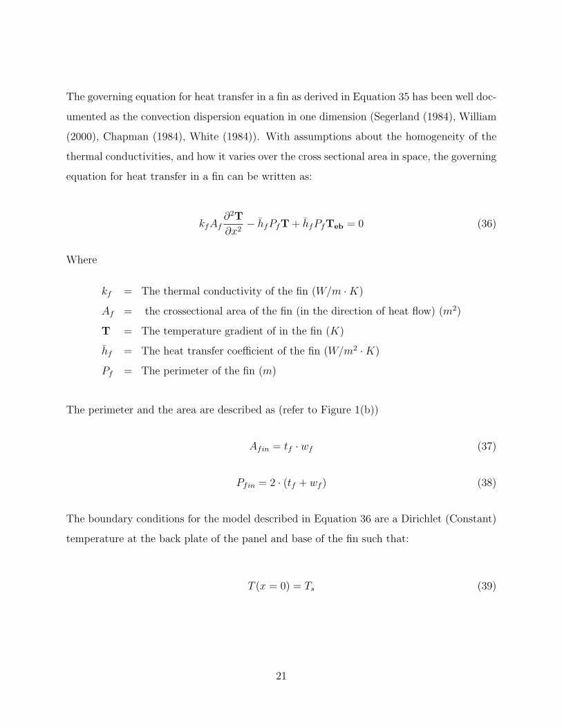
The governing equation for heat transfer in a fin as derived in Equation 35 has been well doc-

umented as the convection dispersion equation in one dimension (Segerland (1984), William

(2000), Chapman (1984), White (1984)). With assumptions about the homogeneity of the

thermal conductivities, and how it varies over the cross sectional area in space, the governing

equation for heat transfer in a fin can be written as:

kfAf∂2T

∂x2− h̄fPfT + h̄fPfTeb = 0 (36)

Where

kf = The thermal conductivity of the fin (W/m · K)

Af = the crossectional area of the fin (in the direction of heat flow) (m2)

T = The temperature gradient of in the fin (K)

h̄f = The heat transfer coefficient of the fin (W/m2 · K)

Pf = The perimeter of the fin (m)

The perimeter and the area are described as (refer to Figure 1(b))

Afin = tf · wf (37)

Pfin = 2 · (tf + wf ) (38)

The boundary conditions for the model described in Equation 36 are a Dirichlet (Constant)

temperature at the back plate of the panel and base of the fin such that:

T (x = 0) = Ts (39)

21

There is a Nuemann flux boundary condition at the end of the fin that describes the heat

loss due to convection by Newton’s Law of cooling such that:

−kAdT

dx= hA(Tb − Tf ) (40)

Where Tb is the Temperature at the end of the fin.

The analytical solution to Equation 36 has been shown by many and is derived in detail in

Appendix 1 using the derivation from William (2000). It is left to the reader to show that

the analytical solution to Equation 36 is as follows:

qfin = kAf (Ts − Teb)

√hfPf/kfAf tanh(L

√hfPf/kfAf ) (41)

5.6 Galerkin Finite Element Solution

Galerkin Finite element scheme is a method of solving PDEs by turning them into a system

of linear equations. As in other types of methods used to do the same thing such as finite

difference and linearization techniques the system is defined as an array of nodal points.

However, the method of finite elements differs from a finite difference scheme, which assumes

that the temperature gradient in between nodes is the arithmetic average of the two nodes

surrounding it. The finite element methodology incorporates weighting or basis functions and

integrates between nodes. The Galerkin Finite element technique uses the basis functions as

the weighting function Table 5.1. This methodology can be applied to solving Equation 36

by piecewise defining the integrals over the entire region Equation 42.

I =

∫ L

0

Ni(x)£(T )dx = 0 (42)

22

where Ni is the weighted shape function or basis function. The integral in Equation 42 is

piecewise defined over the entire domain of the field such that

Ie =∑

`

∫ Le

0

Ni£(T )dx (43)

Where Ie is the integral of the function shown in Equation 42 for a single element. Equation

36 can be rearranged for a finite element solution in the form

£(T) = kfAf∂2T

∂x2− hPfT + hfPfTeb = 0 (44)

With the assumption that T is a function of the basis functions (Equation 45) the integrations

can be evaluated.

T = T̂ = NT̃ (45)

The N vector contains the basis functions for the discritized region. The basis functions used

in this model are cubic, quadratic linear (chapeau) weighting functions (Table 5.1). The basis

functions are written such that there is a transformation from the global coordinate system in

X and transformed to a local natural coordinate system in ξ. For the mathematics behind

this transformation refer to Segerland (1984). For the remainder of this paper the basis

functions will be referenced in ξ.

23

Table 5.1: Finite element basis function descriptions.

Type of element Physical Model Basis function

Linear simplexbi

ξ

bj Ni = 1

2(1 − ξ)

Nj = 12(1 + ξ)

Ni = −12ξ(1 − ξ)

Quadratic simplexbi

ξ

bj

bk Nj = 1 − ξ2

Nk = 12ξ(1 + ξ)

Ni = − 116

(1 + 3ξ)(1 − 3ξ)(1 − ξ)

Cubic elementbi

ξ

bj

bk

bl Nj = 9

16(1 + ξ)(1 − 3ξ)(1 − ξ)

Nk = 916

(1 + ξ)(1 + 3ξ)(1 − ξ)

N` = − 116

(1 + ξ)(1 + 3ξ)(1 − 3ξ)

The region of the fin is discritized into a series nodal points Figure 5.1. The elements are

the spaces between the nodes to which the basis functions are applied.

Fig. 5.1: Nodal breakdown of the fin shown in Figure 4.1. Elements in theregion are described by e1 · · · en and nodal points are described by n1 · · ·nn

.

24

The elemental matrix formulation utilizes Gauss Lagrange Quadrature integration to perform

the integrations. The global matrix equations are formulated following the order presented

in Equation 46 (For the derivation of the matrix equations, and a more in-depth description

of Gauss Lagrange Quadrature refer to Segerland (1984)). It is left to the reader to refer

to Segerland (1984), or Willis and Yeh (1987) for further description of the finite element

solution technique and its application.

A, B =

I I 0 0

I I + II II 0

0 II II + III III

0 0 III III

(46)

25

6 Computer Algorithm

The system of equations 3 – 15, plus the heat transfer in the fins, is solved using an iterative

procedure. Two initial guesses of the temperature of the substrate (Ts) as T1 and T2 are

inserted into the model to get the secant method started. The secant subroutine commu-

nicates with the the energy balance function that systematically solves Equation 2 through

Equation 14. The function needs information about the heat loss in the fin from the finite

element solution as well as information from the interpolation scheme described for the heat

transfer coefficients for the front plate, back plate and the fin. The value of the function is

checked against divergence, slow progress, and a maximum iterations criteria in secant. This

process is repeated until the solution is found or the model produces unrealistic results and

stops. Figure 6.2 shows the computer algorithm in detail.

Program BlockInputs: T1 and T2Outputs: T1 and T2

Secant MethodInputs: T1 and T2Outputs: T1' and T2'

Fin Finite ElementInputs: T1' and T2'Outputs: qf1' and qf2'

Global Module

Variable Storage

Output Files

Outputs: qs, Ts, Tc, Pe

Energy BalanceInputs: T1' and T2'Outputs: qs, Ts, Tc, Pe

Linear InterpolationInputs: T1' and T2'Outputs: hx1' and hx2'

Do For

Fig. 6.2: Computer flow diagram detailing the progression of events for the solutionto the heat transfer in the PV system.

.

26

7 Results and Discussion

The results of this investigation show how changes in the decision variables effect the state

variables of interest. To examine the effects of changing parameters that had to do with the

physical system, the fluid velocity in the duct, fin thickness, fin spacing, fin material, and

fin length were varied over a range of values (Figure 7.1).

It is observed in Figure 7.1 (a) that the cell temperature (Tc) decreases as the cooling air

velocity increases. This causes the panel efficiency (ηpv) to increase. At approximately 8 m/s

the flow becomes turbulent. This causes an even greater change in ηpv and Tc than observed

in the laminar flow region. However, the high velocity that causes transition to turbulence

cannot be reached in practice due to the greater load of the pump associated with such high

speeds. The parasitic load of the cooling duct pump was not considered in this investigation.

If turbulent flow conditions were able to be induced by some other means, there would be a

gain in ηpv. The addition of netting over the ends of the duct, as suggested by Brinkworth

(2006), has the effect of inducing turbulence and preventing birds from entering the duct.

Varying the fin thickness over a range of 0-0.5m indicated that this is a parameter that

has little effect on the performance of the panel (Figure 7.1 (b)). Panel efficiency only had

a change over this range of 9.6 to just about 10%. This result has design application by

allowing the designer to minimize materials needed for the fins.

27

Effect of Coolant Velocity on Panel Operation

9

9.5

10

10.5

11

11.5

0 1 2 3 4 5 6 7 8 9

Fluid Velocity (m/s)

Pane

l Eff

icie

ncy

(%)

35

40

45

50

55

60

65

70

75

Cel

l Tem

pera

ture

s (C

)

Panel Efficiency (%) Cell Temperature (C)

(a) Cooling Fluid Velocity

Effect of Fin Thickness on Panel Operation

9

9.5

10

10.5

11

11.5

0 0.01 0.02 0.03 0.04 0.05 0.06

Fin Thickness (m)

Pane

l Eff

icie

ncy

(%)

35

40

45

50

55

60

65

70

75

Cel

l Tem

pera

ture

(C)

Panel Efficiency (%) Cell Temperature (C)

(b) Fin Thickness

Effect of Fin Spacing on Panel Operation

9

9.5

10

10.5

11

11.5

0 0.05 0.1 0.15 0.2 0.25 0.3

Fin Spacing (m)

Pane

l Eff

icie

ncy

(%)

35

40

45

50

55

60

65

70

75

Cel

l Tem

pera

ture

(C)

Panel Efficiency (%) Cell Temperature (C)

(c) Fin Spacing

Chart_fl

Page 1

Effect of Fin Length on Panel Operation

9

9.5

10

10.5

11

11.5

0 0.05 0.1 0.15 0.2 0.25 0.3 0.35 0.4 0.45 0.5

Fin Length (m)

Pane

l Eff

icie

ncy

(%)

35

40

45

50

55

60

65

70

75

Cel

l Tem

pera

ture

(C)

Panel Efficiency (%) Cell Temperature (C)

(d) Fin Length

Fig. 7.1: Effect of Single Parameter Change on Panel Efficiency and Cell Temperature

28

Fin spacing (Figure 1(c)) appears to have the greatest effect on ηpv and Tc. However, these

results overestimate the benefits as the fin spacing decreases. This is because the 1-d model

was unable to account for overlapping thermal boundary layers that would appear between

fins.

As the fin length (Figure 1(d)) increases, ηpv increases and Tc decreases. In order to use this

correlation for design purposes, a maximum fin length should be set. This maximum will

change depending on the system, such as applications that have a finite length on the back

of the panel that the fins can occupy.

Figure 7.2 gives the change in panel power (Pe) and heat flux into the cooling duct (qduct)

as the decision variables are perturbed.

The greater the velocity of the coolant the higher Pe and qduct. These results are inversely

related to cell temperature. This makes sense because the heat lost from the cell layer

is removed to the duct. The transition from laminar to turbulent flow conditions is also

observed at 8 m/s. This supports the idea that an induced turbulent flow in the cooling duct

has the potential to increase the overall power produced by the system. The fin thickness has

little effect on Pe and qduct. Fins that are more closely separated give the best Pe. However,

the same issue appears at small spacings as was observed for ηpv and Tc. Again, the model

assumptions overestimate the ability of the fins to remove heat from the panel. There is a

positive correlation between fin length, Pe,and qduct. Again, this means that the fin length

should be maximized to the boundary of its feasible length for the given application in order

to maximize panel power.

29

Effect of Coolant Velocity on Panel Operation

90

95

100

105

110

115

120

125

0 1 2 3 4 5 6 7 8 9

Fluid Velocity (m/s)

Pane

l Pow

er (W

)

200

300

400

500

600

700

800

q D

uct (

W)

Panel Power (W) q Duct (W)

(a) Cooling Fluid Velocity

Effect of Fin Thickness on Panel Operation

90

95

100

105

110

115

120

125

0 0.01 0.02 0.03 0.04 0.05 0.06

Fin Thickness (m)

Pane

l Pow

er (W

)

200

300

400

500

600

700

800

q D

uct (

W)

Panel Power (W) q Duct (W)

(b) Fin Thickness

Effect of Fin Spacing on Panel Operation

90

95

100

105

110

115

120

125

0 0.05 0.1 0.15 0.2 0.25 0.3

Fin Spacing (m)

Pane

l Pow

er (W

)

200

300

400

500

600

700

800

q D

uct (

W)

Panel Power (W) q Duct (W)

(c) Fin Spacing

Effect of Fin Length on Panel Operation

90

95

100

105

110

115

120

125

0 0.05 0.1 0.15 0.2 0.25 0.3 0.35 0.4 0.45 0.5

Fin Length (m)

Pane

l Pow

er (W

)

200

300

400

500

600

700

800

q D

uct (

W)

Panel Power (W) q Duct (W)

(d) Fin Length

Fig. 7.2: Effect of Single Parameter Change on Panel Power and q Duct

30

The change in the state variables observed by increasing the magnitude of incoming radiant

energy with a concentrator over a range of magnitudes is given in Figure 7.3. Figure 3(a)

gives the apparent relation between panel efficiency and cell temperature, which is the result

of the linear equation that uses Tc to calculate ηpv (Equation 7).

In Figure 3(b) there is observed to be an optimal concentration at about 3 suns that maxi-

mizes Pe. However, this maximum falls outside of the typical operating temperature of solar

panels and may cause degradation of the cell over time.

An optimization of the system could be performed given realistic limits on the decision

variables. For fin thickness and length, the optimal value lies at this upper limit. The tradeoff

between increased velocities of the cooling air and parasitic pump load would need to be

investigated. The optimal fin width could then be set based on the other fixed parameters.

Then, the optimal concentration magnitude could be determined that satisfies an upper

bound on the temperature at which the cell begins to degrade.Effect of Concentration on Panel Operation

33.5

44.5

55.5

66.5

77.5

88.5

99.510

10.511

11.512

0 0.5 1 1.5 2 2.5 3 3.5 4

Concentration

Pane

l Eff

icie

ncy

(%)

20

40

60

80

100

120

140

Cel

l Tem

pera

ture

(C)

Panel Efficiency (%) Cell Temperature (C)

(a) Panel Efficiency and Cell Temperature

Effect of Concentration on Panel Operation

0

20

40

60

80

100

120

140

160

180

200

0 0.5 1 1.5 2 2.5 3 3.5 4

Concentration

Pane

l Pow

er (W

)

0

200

400

600

800

1000

1200

1400

1600

1800

2000

q D

uct (

W)

Panel Power (W) q Duct (W)

(b) Panel Power and q Duct

Fig. 7.3: Effect of Solar Concentration on Panel Operation

The effect of changing the fin material can be seen in Figure 7.4. The default assumption

is a fin made of aluminum nitride, with a thermal conductivity of 120 W/mK. Increasing

31

the conductivity above this value increases the power output of the panel less than one-half

percent. Decreasing the conductivity to the range of a poor metal conductor decreases panel

output one or two percent.

Fig. 7.4: Effect of Fin Material Conductivity on Panel Operation

8 Conclusions

· Induced turbulent flow in the cooling duct causes greater heat transfer from the panel,

which increases the panel’s electrical output and efficiency.

· Increasing the fin thickness over 1 cm has a negligible effect on panel power and efficiency.

· An optimal concentrator magnitude exists for a system with limits on the decision variables

and cell operating temperature.

· Changing the fin conductivity has little impact on panel output.

32

Appendix 1

A.1.1 Analytical Solution Derivation

d2θ

dx2− n2θ = 0 (47)

has the general solution

θ = C1 cosh(nx) + C2 sinh(nx) (48)

Boundary conditions are T = Tw at x = 0 and dTdx

= 0 at x = L (no heat transferred across

the tip). In terms of θ, the boundary conditions are θw = Tw − T∞ at x = 0 and dθdx

= 0 at

x = L. Applying the first boundary condition gives

θ = C1 cosh(nx) + C2 sinh(nx) (49)

θw = C1(1) + C2(0)

C1 = θw

differentiating θ with respect to x

dθ

dx= θwn sinh(nx) + C2n cosh(nx) (50)

applying the second boundary condition

0 = θwn sinh(nL) + C2n cosh(nL)

33

and

C2 = −θw sinh(nL)

cosh(nL)

the solution becomes

θ

θw

=cosh(nL) cosh(nx) − sinh(nL) sinh(nx)

cosh(nL)(51)

Using Fourier’s law

qx = −kAdθ

dx|x=0 (52)

Equation 51 differentiated and substituted into equation 52 gives

qx = − kAθw

cosh(nL)∗ [n cosh(nL) sinh(nx) − n sinh(nL) cosh(nx)]|x=0 (53)

= − kAθw

cosh(nL)[n(0) − n sinh(nL)]

simplifying

qx = kAnθw tanh(nL) (54)

and in terms of the original parameters

qx = kA(Tw − T∞)

√hcP/kA tanh(L

√hcP/kA) (55)

34

References

Began Adrian, Michael Moran, G. T. (1996). Thermal Design and Optimization. John Wiley

and Sons, Inc.

Brinkworth, B. (2006). “Optimum depth for PV cooling ducts.” Solar Energy, 80, 1131–1134.

Brinkworth, B. and Sandberg, M. (2006). “Design procedure for cooling ducts to minimise

efficiency loss due to temperature rise in PV arrays.” Solar Energy, 80, 89–103.

Chapman, A. J. (1984). Heat Transfer. Macmillan Publishing Company, New York.

F. deWinter, ed. (1990). Solar Collectors, Energy Storage, and Materials. The MIT Press.

Duffie, J. A. and Beckman, W. A. (1991). Solar Engineering of Thermal Processes. John

Wiley and Sons, Inc.

Florschuetz, L. W. (1976). “Extension of the Hottel-Whillier-Bliss model to the analysis of

combined photovoltaic/thermal flat plate collectors.” Photovoltaics and Materials.

Krauter, S. (2004). “Increased electrical yield via water flow over the front of photovoltaic

panels.” Solar Energy Materials & Solar Cells, 82, 131–137.

Meneses-Rodriguez, D., Horley, P. P., Gonzalez-Hernandez, J., Vorobiev, Y. V., and Gor-

ley, P. N. (2005). “Photovoltaic solar cells performance at elevated temperatures.” Solar

Energy, 78, 243–250.

Royne, A., Dey, C. J., and Mills, D. R. (2005). “Cooling of photovoltaic cells under concen-

trated illumination: a critical review.” Solar Energy Material & Solar Cells, 86, 451–483.

Sala, G. (1989). Solar Cells and Optics for Photovoltaic Concentration, 239–267. Adam

Hilger, Bristol and Philadelphia.

Segerland, L. J. (1984). Applie Finite Element Analysis. John Wiley and Sons, Inc., second

edition.

35

SEI, S. E. I. (2004). Photovoltaics Design and Installation Manual. New Society Publishers.

Thomas, L. C. (1999). Heat Transfer - Professional Version. Capstone Publishing Corpora-

tion.

Tonui, J. and Tripanagnostopoulos, Y. (2006). “Improved PV/T solar collectors with heat

extraction by forced or natural air circulation.” Renewable Energy.

Tripanagnostopoulos, Y., Nousia, T., Souliotis, M., and Yianoulis, P. (2001). “Hybrid pho-

tovoltaic/thermal solar systems, Process heating tip sheet 3.” Pergamon.

Vokas, G., Christandonis, N., and Skittides, F. (2005). “Hybrid photovoltaic-thermal systems

for domestic heating and cooling -A theoretical approach.” Solar Energy, 80, 607–615.

White, F. M. (1984). Heat Transfer. Addison Weslley Publishing Company, Inc.

William, J. S. (2000). Engineering Heat Transfer Second Edition. CRC Press LLC.

Willis, R. and Yeh, W. (1987). Groundwater Systems. Pearson Education Inc.

W.J., A. and van Genuchten, M. T. (1982). Analytical Solutions of the One-Dimensinoal

Convective-Dispersive Solute Transport Equation. Department of Agriculture.

36