493

Convex hulls, occluding contours, aspectgraphs and the Hough transform1

M. Wright A. Fitzgibbon R. B. FisherDepartment of Artificial Intelligence

University of EdinburghEdinburgh, Scotland EH1 2QL

markwr, andrewfg or rbf@aifh.ed.ac.uk

Abstract

The Hough transform is a standard technique for finding features suchas lines in images. Typically edgels or other features are mapped intoa partitioned parameter or Hough space as individual votes. The tar-get image features are detected as peaks in the Hough space. In thispaper we consider not just the peaks but the mapping of the entireshape boundary from image space to the Hough parameter space. Weanalyse this mapping and illustrate correspondences between featuresin Hough space and image space. Using this knowledge we presentan algorithm to construct convex hulls of arbitrary 2D shapes withsmooth and polygonal boundaries as well as isolated point sets. Wealso demonstrate its extension to the 3D case. We then show how thismapping changes as we move the origin in image space. The origincan be considered as a vantage point from which to view the objectand the occluding contour can be extracted easily from Hough space asthose points where R = 0. We demonstrate the potential for trackingof transitions in the mapping to be used to construct an aspect graphof arbitrary 2D and 3D shapes.

1 Introduction

The Hough transform [2] is a standard technique in computer vision having manyapplications for finding lines, circles and other features in images [3]. Typicallyedgels or other features are mapped into a partitioned parameter or Hough spaceas individual votes. The target image features are detected as peaks in the Houghspace.

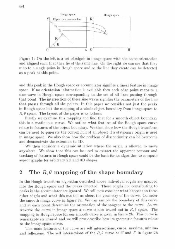
One particular variant of the Hough transform for line detection is shown infigure 1. This uses the R6 parameterization and makes use of edgel orientation toreduce computation [4]. For each edgel a perpendicular is dropped from the originin image space to a line passing through the edgel and with the same orientation.This is then mapped to a space with two parameters R and 9 where R is thelength of perpendicular and 6 is the angle it makes with the araxis. As orientationinformation is avialable then each edgel maps to a single point in Hough space. Ifthe edgels he on a line then all will map to a common point in the Hough space

lThis work was funded by EPSRC grant number GR/J44018

BMVC 1995 doi:10.5244/C.9.49

494

Image space Hough spaceEdgels on a common line R

0 x 0 eFigure 1: On the left is a set of edgels in image space with the same orientationand aligned such that they lie of the same line. On the right we can see that theymap to a single point in Hough space and so the line they create can be detectedas a peak at this point.

and this peak in the Hough space or accumulator signifies a linear feature in imagespace. If no orientation information is available then each edge point maps to asine wave in Hough space corresponding to the set of all lines passing throughthat point. The intersection of these sine waves signifies the parameters of the linethat passes through all the points. In this paper we consider not just the peaksin Hough space but the mapping of a whole object boundary from image space toR, 9 space. The layout of the paper is as follows:

Firstly we examine this mapping and find that for a smooth object boundarythis is a continuous curve. We outline what features of the Hough space curverelate to features of the object boundary. We then show how the Hough transformcan be used to generate the convex hull of an object if a stationary origin is usedin image space. We also show how the problem of discontinuity can be overcomeand demonstrate the extension to 3D.

We then consider a dynamic situation where the origin is allowed to moveanywhere. We show that this can be used to extract the apparent contour andtracking of features in Hough space could be the basis for an algorithm to computeaspect graphs for arbitrary 2D and 3D shapes.

2 The i?, 0 mapping of the shape boundary

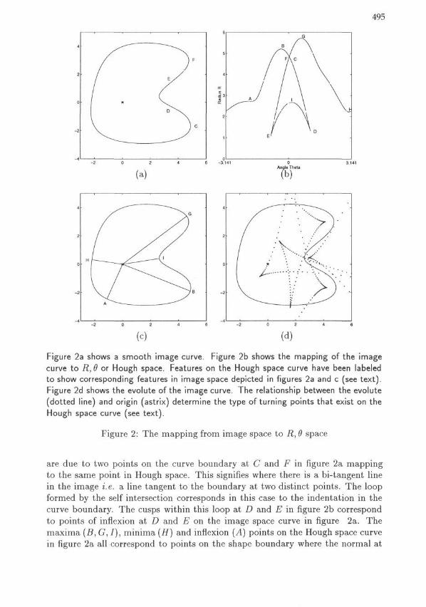
In the Hough transform algorithm described above individual edgels are mappedinto the Hough space and the peaks detected. Those edgels not contributing topeaks in the accumulator are ignored. We will now consider what happens to theseother edgels and what this can tell us about the geometry of the curve. Considerthe smooth image curve in figure 2a. We can sample the boundary of this curveand at each point determine the orientation of the tangent to the curve. As wetraverse the curve in image space a curve is also traced out in R, 6 space. Themapping to Hough space for our smooth curve is given in figure 2b. This curve isremarkably structured and we will now describe how its geometric features relateto the image space curve.

The main features of the curve are self intersections, cusps, maxima, minimaand inflexions. The self intersections of the R, 6 curve at C and F in figure 2b

495

(c (d)

Figure 2a shows a smooth image curve. Figure 2b shows the mapping of the imagecurve to R, 6 or Hough space. Features on the Hough space curve have been labeledto show corresponding features in image space depicted in figures 2a and c (see text).Figure 2d shows the evolute of the image curve. The relationship between the evolute(dotted line) and origin (astrix) determine the type of turning points that exist on theHough space curve (see text).

Figure 2: The mapping from image space to R, 9 space

are due to two points on the curve boundary at C and F in figure 2a mappingto the same point in Hough space. This signifies where there is a bi-tangent linein the image i.e. a line tangent to the boundary at two distinct points. The loopformed by the self intersection corresponds in this case to the indentation in thecurve boundary. The cusps within this loop at D and E in figure 2b correspondto points of inflexion at D and E on the image space curve in figure 2a. Themaxima (B, G, I), minima (H) and inflexion (̂ 4) points on the Hough space curvein figure 2a all correspond to points on the shape boundary where the normal at

496

that point passes through the origin as shown in figure 2c. It is a minima if thedistance along the the normal measured from the shape boundary to the originis less than the radius of curvature of the curve at that point. It is a maxima ifthe normal length is greater than the radius of curvature and it is an inflexion ifthey are equal. The locus of centres of curvature defines a cusped curve called theevolute which is depicted over the shape boundary as a dotted line in figure 2d.So the minima correspond to an origin within the evolute, maxima have an originbeyond the evolute and inflexions occur when the origin is on the evolute.

3 The R, 0 mapping and convex hullThe relationship between the R, 9 mapping and the convex hull is as follows. If wetake for every value of 9 that portion of the Hough space curve that has maximumR i.e. the upper envelope of the R, 9 space graph. Then the corresponding pointsin image space are those points on the convex hull.

3.1 Dealing with discontinuity

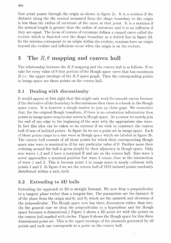
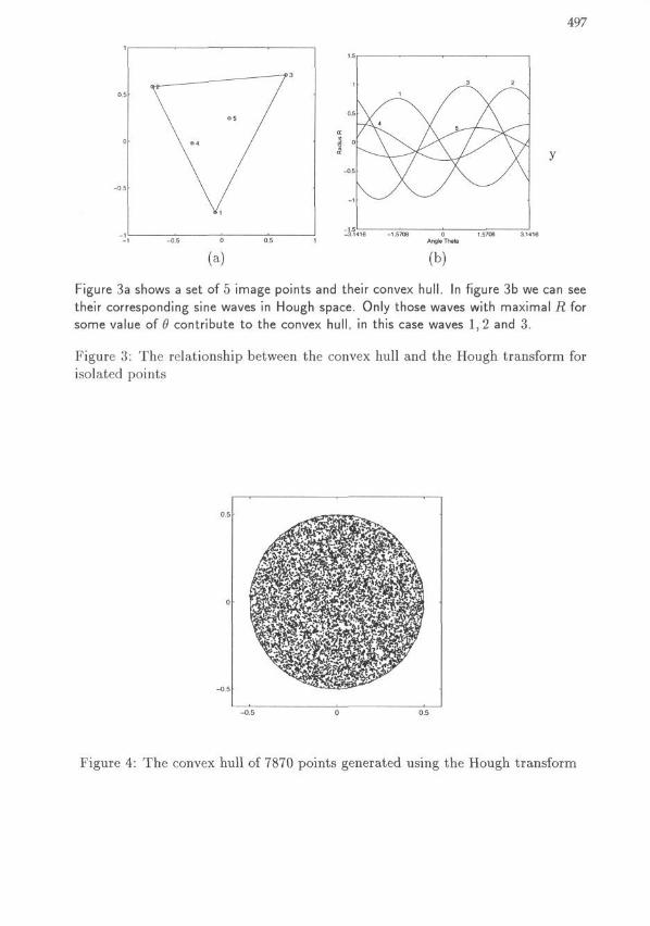
It would appear at first sight that this might only work for smooth curves becauseif the derivative of the boundary is discontinuous then there is a break in the Houghspace curve. It is however a simple matter to join up these gaps. We rememberthat, for the original Hough transform, if there is no orientation information thenpoints in image space map to sine waves in Hough space. At a corner we merely jointhe end of one edge to the beginning of the next with the appropriate sine wave.In fact this idea can be taken to its extreme if we wish to construct the convexhull of sets of isolated points. In figure 3a we see a point set in image space. Eachof these points maps to a sine wave in Hough space which are labeled in figure 3b.The convex hull consists of all those points for which their corresponding Houghspace sine wave is maximal in R for any particular value of 9. Further more theirordering around the hull is given simply by their adjacency in Hough space. Onlysine waves 1, 2 and 3 have a maximal R and are on the convex hull. Sine wave 5never approaches a maximal position but wave 4 comes close at the intersectionof wave 1 and 2. This is because point 4 in image space is nearly collinear withpoints 1 and 2. In figure 4 we see the convex hull of 7870 isolated points randomlydistributed within a unit circle.

3.2 Extending to 3D hulls

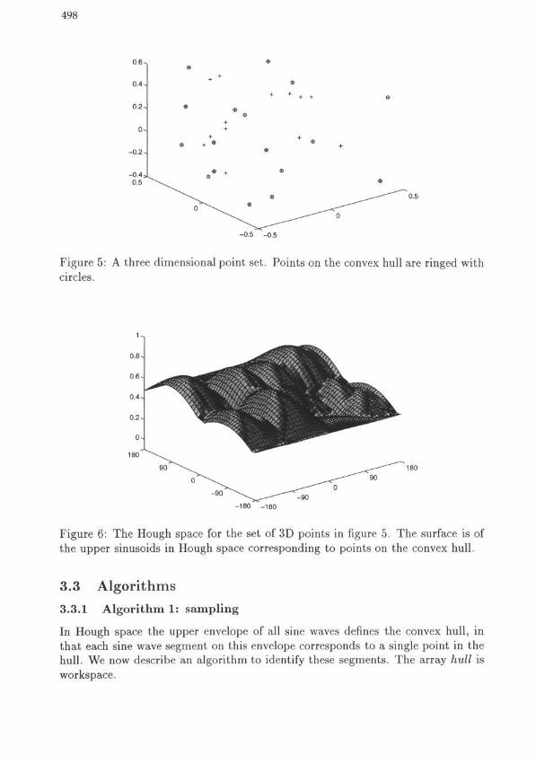
Extending the approach to 3D is straight forward. We now drop a perpendicularto a tangent plane rather than a tangent line. The parameters are the distance Rof the plane from the origin and 6\ and #2 which are the azimuth and elevation ofthe perpendicular. The Hough space now has three dimensions rather than two.(In the general case we drop the perpendicular to a hyperplane and the Houghspace becomes n-dimensional.) Figure 5 shows a 3D point set with the points onthe convex hull marked with circles. Figure 6 shows the Hough space for this threedimensional point set. This is the upper envelope of the sinusoids generated by allpoints and each one corresponds to a point on the convex hull.

497

Figure 3a shows a set of 5 image points and their convex hull. In figure 3b we can seetheir corresponding sine waves in Hough space. Only those waves with maximal R forsome value of 6 contribute to the convex hull, in this case waves 1,2 and 3.

Figure 3: The relationship between the convex hull and the Hough transform forisolated points

0.5

0

-0.5

In$ggj

Figure 4: The convex hull of 7870 points generated using the Hough transform

498

0.6 v

0.4-

0.2^

e+ +

-0.2 ~

-0.5 -0.5

Figure 5: A three dimensional point set. Points on the convex hull are ringed withcircles.

90

-180 -180

Figure 6: The Hough space for the set of 3D points in figure 5. The surface is ofthe upper sinusoids in Hough space corresponding to points on the convex hull.

3.3 Algorithms

3.3.1 Algorithm 1: sampling

In Hough space the upper envelope of all sine waves defines the convex hull, inthat each sine wave segment on this envelope corresponds to a single point in thehull. We now describe an algorithm to identify these segments. The array hull isworkspace.

499

Step 1 Let pi(O),... ,pn(9) be the sine waves in Hough space corresponding tothe n points in the image space.

Step 2 Set index k to 1; for 9 = 0 to 2n in steps of A$ (see discussion below) fillan array hull[k] with indicies as follows:

Step 2a Find the greatest sine at this 9: Set hull[k] := i where pt(0) > Pj(9)for all 1 < j < n.

Step 2b Increment index k by 1.

Step 3 The distinct indicies in hull are those points in the image plane in theconvex hull.

(Termination is trivial since A# > 0.)An important issue is the granularity of the Hough space from the viewpoint

of the complexity of computing the convex hull by this algorithm. Consider threecollinear points a, b and c, with a and b in the convex hull, and c lying betweenthem. Without loss of generality we assume that c lies at the origin of the imageplane and a and b on either side of it along the z-axis, at — xa and x^. We willconsider the behaviour in Hough space as c is perturbed along the j/-axis by 8c,and derive from this the required sampling interval of the Hough space so as todetect that c is now part of the hull.

Perturbing c in this way contributes 8 c. sin 9 to Hough space, and we see thatthe interval A# must be such that

As < ta,n~1(8c/xa) + ta.n~1(8c/xb)

for c to be seen to be in the hull. This gives an approximate complexity O( t an-"(i/p))where p measures the greatest distance between any two points a and 6. Choosingp a priori to be the image diagonal renders it independant from (a bounded) n,and overall complexity is O(n); however, constants are much greater than in theGraham's scan algorithm [1] [6].

For example, for a 512 x 512 image we have 512.47rn for n points with a twice-over sampling interval.

3.3.2 Algorithm 2: non-sampling

We can make a significant (see below) average-case improvement in speed of thealgorithm, with the following approach, which has complexity O(n2). (We adoptthe same notation as above.)

Step 1 Determine i such that p,-(0) > Pj{0) for all 1 < j < n. We use this hullpoint to start.

Step 2 Record that the point i is on the hull. If i = 2TT then we have completedthe hull, so stop.

Step 3 Compute the next point i' known to be on the hull as follows. Determinethe smallest Of such that £>*(#;<) = Pi'{9v) subject to 0,-/ > 9{. i' is the'nearest' sine wave which intersects with since wave i.

Set i to 'i and go to Step 2.

500

(We omit proofs of termination.)This algorithm has quadratic complexity since there are n computations in

Step 3 (finding the next interection point), and we do this for each point in thehull, which is O(n) (think of all n points arranged as as circle). Hence O(n2).

However, we anticipate much better that this worst-case performace in practice,since typically considerably fewer points are in the hull in comparision with n.

4 The i?, 9 mapping and aspect graphIn the last section we computed the convex hull of 2D and 3D objects by usingthe R, 9 mapping of object boundaries with a stationary origin in image space. Inthis section we consider what happens to the same mapping as we move the originin image space.

If the origin is outside the shape then we can consider it as a vantage point fromwhich we look at the object. Using this perspective the first striking observation isthat the occluding contour of the object, i.e. those point where the local tangentline or plane lies along the line of sight, is simply those points where R — 0.Further more those points with R > 0 have normals pointing toward the origin orvantage point and those with R < 0 have normals points away. We suggest thatthese observations can form the basis of an algorithm to build aspect graphs [5]of arbitrary 2D and 3D shapes. We can move the origin about the viewing sphereand keep track of the self intersections and cusps of the Hough space curve. Asthese features cross the 9 axis i.e. R = 0 these constitute event boundaries inthe aspect graph. To illustrate this principle we have devised a graphics programwhich animates in real time the mapping from image space to Hough space as theorigin is moved or the shape boundary is deformed. Figure 7 shows a few differentframes of the animation. As the vantage point (cross) is moved so the concavitycomes into view the self intersection and cusps of the curve in Hough space movebelow the 9 axis. We suggest that tracking of these events could be used to triggerthe building of new branches and nodes in the aspect graph.

5 DiscussionThe convex hull algorithms presented above has similarities to Graham's algo-rithm where points are sorted according to angle. The complexity of Graham'salgorithm is 0(n\n(n)). However our Hough based approach (algorithm 1) has ahigh constant term due to the sampling of Hough space. Algorithm 2 has muchpoorer worse case complexity but in the average case we anticipate better perfor-mance than algorithm 1. Neither algorithm can compete with Graham's algorithmin performance as a practical convex hull algorithm. However, our goal was notto produce an efficient new algorithm but to investigate the relationship betweenthe convex hull and the Hough transform.

We believe that sampling may also be the basis for producing approximateconvex hulls (and aspect graphs) in a principled way which has been identified asan important problem. Unlike Graham's algorithm there is a global representationof the hull. We could in principle use this to assess the effect of leaving out a

501

Figures 7a,c and e show a kidney bean shape in image space where different viewpoints are marked with a cross. In figure 7a no part of the concavity can be seen andthe loop in Hough space in figure 7b is above the x axis. In figure 7c the viewpoint isprecisely along the bi-tangent line, this is signified by the self intersection in figure 7dcrossing the x axis. In figure 7e the concavity is in plain view and the loop in figure 7fis below the x axis.

Figure 7: The transitions in Hough space relating to changing view point.

502

particular point. This could be on the principle of the area of the sine wave forwhich it is maximal in R.

The Hough approach to building the aspect graph has the problem that al-though we can tell if a face points towards the viewer we cannot tell if it is occludedby another part of the object. It is as if we are considering the singularities of atransparent object. We could solve this by filtering the Hough space output withsome kind of visibility check. One such check would be to compute a differenttransform, say d, a where d is the length of a line from the boundary point to theorigin and a is the angle this line makes with the x axis. The points in d, a spacewith minimal d for a particular a are those points which are unoccluded.

6 Conclusions

We have considered the mapping of object boundaries using the Hough transformsR, 9 parameterization. We have shown the correspondence of features in Houghspace to image space. This information has been used to construct an algorithmto compute 2D and 3D convex hulls. We considered the effect of moving theorigin and demonstrated the potential of the approach to compute aspect graphsof arbitrary shapes. We hope that we have challenged the traditional role of theHough transform an purely a feature detector. Clearly the local structure anddynamics of this mapping can tell us alot about the geometry of shapes aroundus.

References

[1] R. L. Graham. An efficient algorithm for determining the convex hull of a finiteplanar set. Information processing letters, 1:132-133, 1972.

[2] P. V. C. Hough. Method and means for recognising complex patterns. USPatent 3069654, 1962.

[3] J. Illingworth and J. Kittler. A survey of the Hough transform. CVGIP,44:87-116, 1988.

[4] C. Kimme, D. Ballard, and J. Sklansky. Finding circles by an array of acculu-lators. Comm ACM, 18:120-122, 1975.

[5] J. J. Koenderink and A. J. van Doom. The internal representions of solidshape with respect to vision. Biological Cybernetics, 32:211-216, 1979.

[6] J. O'Rourke. Computational geometry in C. Cambridge University press, 1992.