Embed Size (px)
Citation preview

Neil Marks; DLS/CCLRC CAS, Baden bei Wien, September 2004
Conventional Magnets for Accelerators
Neil Marks,DLS/CCLRC,
Daresbury Laboratory,Warrington WA4 4AD,
U.K.Tel: (44) (0)1925 603191Fax: (44) (0)1925 603192

Neil Marks; DLS/CCLRC CAS, Baden bei Wien, September 2004
ContentsThe presentation deals with d.c. magnets only.i) No current or steel:• Laplace's equation with scalar potential;• Cylindrical harmonic solutions in two dimensions;
ii) Introduce steel yoke:• Ideal pole shapes for dipole, quad and sextupole;• Field harmonics-symmetry restraints and significance;
iii) Introduce current:• Ampere-turns in dipole, quad and sextupole;

Neil Marks; DLS/CCLRC CAS, Baden bei Wien, September 2004
Contents (cont.)iv) Magnet geometry:• Backleg and coil geometry- 'C', 'H' and 'window frame'
designs;• Coil economic optimisation-capital/running costs;
v) Field computation and pole optimisation:• Field computation software-OPERA, TOSCA;• Design of pole geometry for dipole, quad and sextupole;• Magnet ends-computation and design;

Neil Marks; DLS/CCLRC CAS, Baden bei Wien, September 2004
Magnets we know about:Dipoles to bend the beam:
Quadrupoles to focus it:
Sextupoles to correct chromaticity:
We need to establish a formal approach to describing these magnets.

Neil Marks; DLS/CCLRC CAS, Baden bei Wien, September 2004
But first – nomenclature!Magnetic Field: (the magneto-motive force produced by electric currents)
symbol is H (as a vector);units are Amps/metre in S.I units (Oersteds in cgs);
Magnetic Induction or Flux Density: (the density of magnetic flux driven through a medium by the magnetic field)
symbol is B (as a vector);units are Tesla (Webers/m2 in mks, Gauss in cgs);
Note: induction is frequently referred to as "Magnetic Field".
Permeability of free space:symbol is µ0 ;units are Henries/metre;
Permeability (abbreviation of relative permeability):symbol is µ;the quantity is dimensionless;

Neil Marks; DLS/CCLRC CAS, Baden bei Wien, September 2004
i) No Currents - Maxwell’s equations:∇.B = 0 ;∇ H = j ;
In the absence of currents: j = 0.
Then we can put: B = - ∇φ
So that: ∇2φ = 0 (Laplace's equation).
Taking the two dimensional case (ie constant in the z direction) and solving for cylindrical coordinates (r,θ):
φ = (E+F θ)(G+H ln r) + Σn=1∞ (Jn r n cos nθ +Kn r n sin nθ
+Ln r -n cos n θ + Mn r -n sin n θ )

Neil Marks; DLS/CCLRC CAS, Baden bei Wien, September 2004
In practical situations:The scalar potential simplifies to:
φ = Σn (Jn r n cos nθ +Kn r n sin nθ),
with n integral and Jn,Kn a function of geometry.
Giving components of flux density:
Br = - Σn (n Jn r n-1 cos nθ +nKn r n-1 sin nθ)Bθ = - Σn (-n Jn r n-1 sin nθ +nKn r n-1 cos nθ)

Neil Marks; DLS/CCLRC CAS, Baden bei Wien, September 2004
SignificanceThis is an infinite series of cylindrical harmonics; they define the allowed distributions of B in 2 dimensions in the absence of currents within the domain of (r,θ).
Distributions not given by above are not physically realisable.
Coefficients Jn, Kn are determined by geometry (iron boundaries or remote current sources).

Neil Marks; DLS/CCLRC CAS, Baden bei Wien, September 2004
Cartesian CoordinatesIn Cartesian coordinates, the components are given by:
rθ
0
BrΒθ
x
y
Bx = Br cos θ - Bθ sin θ,
By = Br sin θ + Bθ cos θ,

Neil Marks; DLS/CCLRC CAS, Baden bei Wien, September 2004
Dipole field: n = 1Cylindrical: Cartesian:Br = J1 cos θ + K1 sin θ; Bx = J1
Bθ = -J1 sin θ + K1 cos θ; By = K1
φ =J1 r cos θ +K1 r sin θ. φ =J1 x +K1 y
So, J1 = 0 gives vertical dipole field:
K1 =0 gives horizontal dipole field.
Bφ = const.

Neil Marks; DLS/CCLRC CAS, Baden bei Wien, September 2004
Quadrupole field: n = 2Cylindrical: Cartesian:Br = 2 J2 r cos 2θ +2K2 r sin 2θ; Bx = 2 (J2 x +K2 y)Bθ = -2J2 r sin 2θ +2K2 r cos 2θ; By = 2 (-J2 y +K2 x)φ = J2 r 2 cos 2θ +K2 r 2 sin 2θ; φ = J2 (x2 - y2)+2K2 xy
J2 = 0 gives 'normal' or ‘right’ quadrupole field.
K2 = 0 gives 'skew' quad fields (above rotated by π/4).
Lines of flux density
Line of constant
scalar potential

Neil Marks; DLS/CCLRC CAS, Baden bei Wien, September 2004
Sextupole field: n = 3Cylindrical; Cartesian:Br = 3 J3r2 cos 3θ +3K3r2 sin 3θ; Bx = 3{J3 (x2-y2)+2K3yx}Bθ= -3J3 r2 sin 3θ+3K3 r2 cos 3θ; By = 3{-2 J3 xy + K3(x2-y2)}φ = J3 r3 cos 3θ +K3 r3 sin 3θ; φ = J3 (x3-3y2x)+K3(3yx2-y3)
Line of constant scalar potential
Lines of flux density
+C
-C
+C
-C
+C
-C J3 = 0 giving 'normal' or ‘right’ sextupole field.+C
-C
+C
-C
+C
-C
Neil Marks; DLS/CCLRC CAS, Baden bei Wien, September 2004
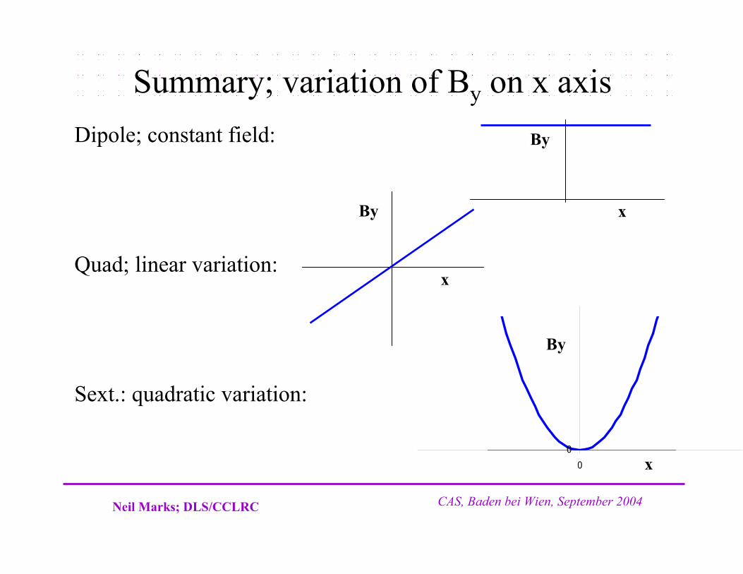
Summary; variation of By on x axisDipole; constant field:
Quad; linear variation:
Sext.: quadratic variation:
x
By
00
By
x
x
By

Neil Marks; DLS/CCLRC CAS, Baden bei Wien, September 2004
Alternative notification (USA)
B (x) = B ρ
k n xn
n!n =0
∞∑
magnet strengths are specified by the value of kn; (normalised to the beam rigidity);
order n of k is different to the 'standard' notation:
dipole is n = 0;quad is n = 1; etc.
k has units:k0 (dipole) m-1;k1 (quadrupole) m-2; etc.

Neil Marks; DLS/CCLRC CAS, Baden bei Wien, September 2004
ii) Introducing Iron YokesWhat is the ideal pole shape?•Flux is normal to a ferromagnetic surface with infinite µ:
•Flux is normal to lines of scalar potential, (B = - ∇φ);•So the lines of scalar potential are the ideal pole shapes!
(but these are infinitely long!)
curl H = 0
therefore ∫ H.ds = 0;
in steel H = 0;
therefore parallel H air = 0
therefore B is normal to surface.
µ = ∞
µ = 0

Neil Marks; DLS/CCLRC CAS, Baden bei Wien, September 2004
Equations for the ideal poleEquations for Ideal (infinite) poles;(Jn = 0) for normal (ie not skew) fields:Dipole:
y= ± g/2;(g is interpole gap).Quadrupole:
xy=±R2/2;Sextupole:
3x2y - y3 = ±R3;
R

Neil Marks; DLS/CCLRC CAS, Baden bei Wien, September 2004
Combined function magnets'Combined Function Magnets' - usually dipole and quadrupole field combined:
A quadrupole magnet withphysical centre shifted frommagnetic centre.
Characterised by 'field index' n,+ve or -ve dependingon direction of gradient;do not confuse with harmonic n!
B
n = - ρΒ 0
∂B∂x
,
ρ is radius of curvature of the beam;
Bo is central dipole field

Neil Marks; DLS/CCLRC CAS, Baden bei Wien, September 2004
Pole equations for c.f. magnetIf physical and magnetic centres are separated by X0
Then B0 = ∂B∂x
X0;
therefore X0 = − ρ / n;
in a quadrupole x' y = ±R2 / 2where x' is measured from the true quad centre;
Put x' = x + X0
So pole equation is y = ± R2
2nρ
1 − nxρ
- 1
or y = ±g 1− nxρ
- 1
where g is the half gap at the physical centre of the magnet

Neil Marks; DLS/CCLRC CAS, Baden bei Wien, September 2004
The practical PolePractically, poles are finite, introducing errors; these appear as higher harmonics which degrade the field distribution.However, the iron geometries have certain symmetries that restrict the nature of these errors.
Dipole: Quadrupole:

Neil Marks; DLS/CCLRC CAS, Baden bei Wien, September 2004
Possible symmetries:Lines of symmetry:
Dipole: QuadPole orientation y = 0; x = 0; y = 0determines whether poleis normal or skew.
Additional symmetry x = 0; y = ± ximposed by pole edges.
The additional constraints imposed by the symmetrical pole edges limits the values of n that have non zero coefficients

Neil Marks; DLS/CCLRC CAS, Baden bei Wien, September 2004
Dipole symmetries
+φ
-φ
Type Symmetry Constraint
Pole orientation φ(θ) = -φ(-θ) all Jn = 0;
Pole edges φ(θ) = φ(π -θ) Kn non-zero only for:n = 1, 3, 5, etc;
So, for a fully symmetric dipole, only 6, 10, 14 etc pole errorscan be present.
+φ +φ

Neil Marks; DLS/CCLRC CAS, Baden bei Wien, September 2004
Quadrupole symmetries
Type Symmetry Constraint
Pole orientation φ(θ) = -φ( -θ) All Jn = 0;
φ(π) = -φ(π -θ) Kn = 0 all odd n;
Pole edges φ(θ) = φ(π/2 -θ) Kn non-zero only for:n = 2, 6, 10, etc;
So, a fully symmetric quadrupole, only 12, 20, 28 etc pole errors can be present.

Neil Marks; DLS/CCLRC CAS, Baden bei Wien, September 2004
Sextupole symmetries
Type Symmetry Constraint
Pole orientation φ(θ) = -φ( -θ) All Jn = 0;φ(θ) = -φ(2π/3 - θ) Kn = 0 for all n φ(θ) = -φ(4π/3 - θ) not multiples of 3;
Pole edges φ(θ) = φ(π/3 - θ) Kn non-zero only for: n = 3, 9, 15, etc.
So, a fully symmetric sextupole, only 18, 30, 42 etc pole errorscan be present.

Neil Marks; DLS/CCLRC CAS, Baden bei Wien, September 2004
iii) Introduction of currentsNow for j ≠ 0 ∇ H = j ;
To expand, use Stoke’s Theorum:for any vector V and a closed curve s :
∫V.ds =∫∫ curl V.dS
Apply this to: curl H = j ;
dS
dsV
then in a magnetic circuit:
∫ H.ds = N I;
N I (Ampere-turns) is total current cutting S

Neil Marks; DLS/CCLRC CAS, Baden bei Wien, September 2004
Excitation current in a dipole
µ >>
g
λ
1
NI/2
NI/2
B is approx constant round the loop made up of λ and g, (but see below);
But in iron, µ>>1,and Hiron = Hair /µ ;
SoBair = µ0 NI / (g + λ/µ);
g, and λ/µ are the 'reluctance' of the gap and iron.
Approximation ignoring iron reluctance (λ/µ << g ):
NI = B g /µ0

Neil Marks; DLS/CCLRC CAS, Baden bei Wien, September 2004
Relative permeability of low silicon steel
10
100
1000
10000
0.0 0.5 1.0 1.5 2.0 2.5
B (T)
µ
Parallel to rolling direction Normal to rolling direction.

Neil Marks; DLS/CCLRC CAS, Baden bei Wien, September 2004
Excitation current in quad & sextupoleFor quadrupoles and sextupoles, the required excitation can be calculated by considering fields and gap at large x. For example: Quadrupole:
y
x B
Pole equation: xy = R2 /2On x axes BY = gx;where g is gradient (T/m).
At large x (to give vertical lines of B):
N I = (gx) ( R2 /2x)/µ0ie
N I = g R2 /2 µ0 (per pole).
The same method for a Sextupole,
( coefficient gS,), gives:
N I = gS R3/3 µ0 (per pole)

Neil Marks; DLS/CCLRC CAS, Baden bei Wien, September 2004
General solution for magnets order nIn air (remote currents! ), B = µ0 H
B = - ∇φIntegrating over a limited path(not circular) in air: N I = (φ1 – φ2)/µoφ1, φ2 are the scalar potentials at two points in air.Define φ = 0 at magnet centre;then potential at the pole is:
µo NI
Apply the general equations for magneticfield harmonic order n for non-skewmagnets (all Jn = 0) giving:
N I = (1/n) (1/µ0) {Br/R (n-1)} R nWhere:
NI is excitation per pole;R is the inscribed radius (or half gap in a dipole);term in brackets {} is magnet strength in T/m (n-1).
y
φ = 0
φ = µ0 NI
Neil Marks; DLS/CCLRC CAS, Baden bei Wien, September 2004
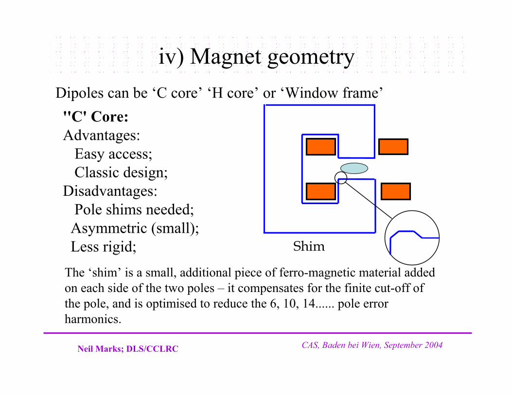
iv) Magnet geometryDipoles can be ‘C core’ ‘H core’ or ‘Window frame’''C' Core:Advantages:
Easy access;Classic design;
Disadvantages:Pole shims needed;Asymmetric (small);Less rigid; Shim
The ‘shim’ is a small, additional piece of ferro-magnetic material added on each side of the two poles – it compensates for the finite cut-off of the pole, and is optimised to reduce the 6, 10, 14...... pole error harmonics.

Neil Marks; DLS/CCLRC CAS, Baden bei Wien, September 2004
A typical ‘C’ cored Dipole
Cross section of the Diamond storage ring dipole.

Neil Marks; DLS/CCLRC CAS, Baden bei Wien, September 2004
H core and window-frame magnets
‘H core’:Advantages:
Symmetric;More rigid;
Disadvantages:Still needs shims;Access problems.
''Window Frame'Advantages:
High quality field;No pole shim;Symmetric & rigid;
Disadvantages:Major access problems;Insulation thickness
Neil Marks; DLS/CCLRC CAS, Baden bei Wien, September 2004
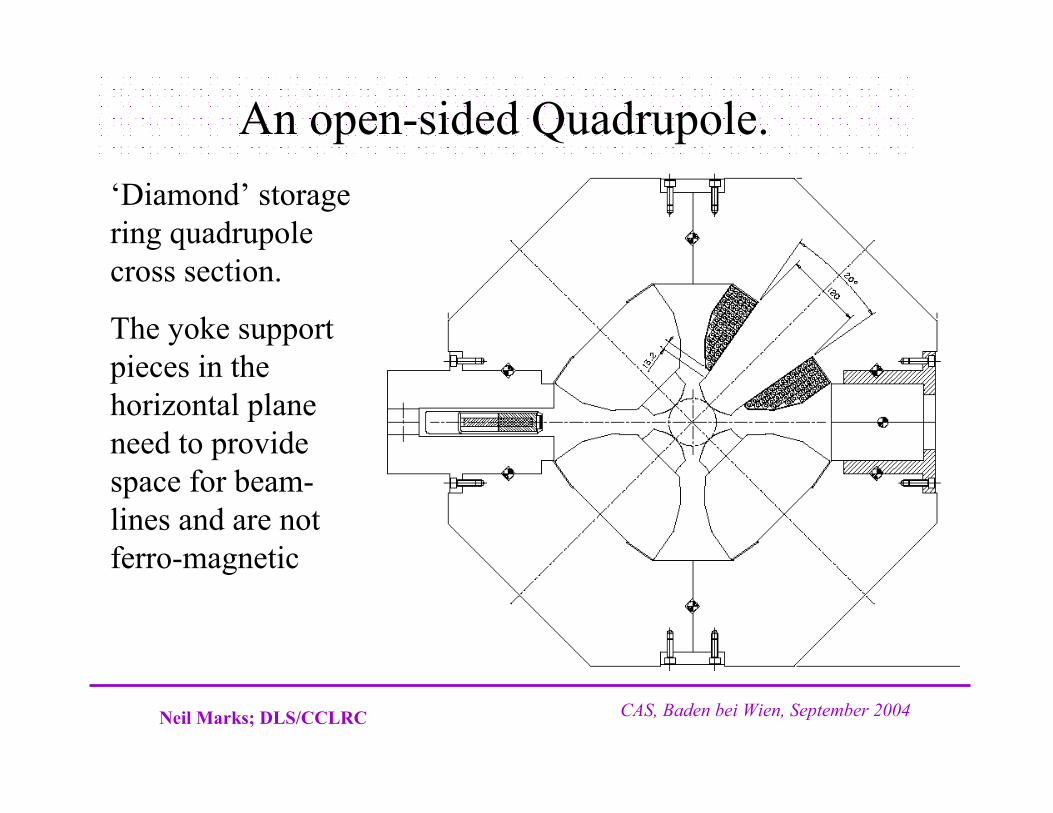
‘Diamond’ storage ring quadrupole cross section.
The yoke support pieces in the horizontal plane need to provide space for beam-lines and are not ferro-magnetic
An open-sided Quadrupole.

Neil Marks; DLS/CCLRC CAS, Baden bei Wien, September 2004
Coil geometry
Standard design is rectangular copper (or aluminium) conductor, with cooling water tube. Insulation is glass cloth and epoxy resin.
Amp-turns (NI) are determined, but total copper area (Acopper) and number of turns (N) are two degrees of freedom and need to be decided.
Current density:j = NI/AcopperOptimum j determined from economic criteria.

Neil Marks; DLS/CCLRC CAS, Baden bei Wien, September 2004
Current density - optimisationAdvantages of low j:• lower power loss – power bill is decreased;• lower power loss – power converter size is decreased;• less heat dissipated into magnet tunnel.
Advantages of high j:• smaller coils;• lower capital cost;• smaller magnets.
Chosen value of j is anoptimisation of magnet capital against power costs.
0.0
0.0 1.0 2.0 3.0 4.0 5.0 6.0
Current density j
Life
time
cost
running
capital
total

Neil Marks; DLS/CCLRC CAS, Baden bei Wien, September 2004
Number of turns, NThe value of number of turns (N) is chosen to match power supply and interconnection impedances.
Factors determining choice of N:Large N (low current) Small N (high current) Small, neat terminals. Large, bulky terminals
Thin interconnections-hence low Thick, expensive connections.cost and flexible.
More insulation layers in coil, High percentage of copper inhence larger coil volume and coil volume. More efficient useincreased assembly costs. of space available
High voltage power supply High current power supply.-safety problems. -greater losses.

Neil Marks; DLS/CCLRC CAS, Baden bei Wien, September 2004
Examples of typical turns/currentFrom the Diamond 3 GeV synchrotron source:Dipole:
N (per magnet): 40;I max 1500 A;Volts (circuit): 500 V.
Quadrupole:N (per pole) 54;I max 200 A;Volts (per magnet): 25 V.
Sextupole:N (per pole) 48;I max 100 A;Volts (per magnet) 25 V.

Neil Marks; DLS/CCLRC CAS, Baden bei Wien, September 2004
v) Pole designTo compensate for the non-infinite pole, shims are added at the pole edges. The area and shape of the shims determine the amplitude of error harmonics which will be present.
A
A
Dipole: Quadrupole:
The designer optimises the pole by ‘predicting’ the field resulting from a given pole geometry and then adjusting it to give the required quality.
When high fields are present,chamfer angles must be small, and tapering of poles may be necessary

Neil Marks; DLS/CCLRC CAS, Baden bei Wien, September 2004
Diamond s.r dipolePole profile, showing shim and Rogowski roll-off for Diamond 1.4 T dipole.:

Neil Marks; DLS/CCLRC CAS, Baden bei Wien, September 2004
Computing magnetic fieldsAdvanced 2 D and 3 D ‘finite element’ codes predicting field distributions between poles and at the magnet ends give accurate predictions of the strength of the magnet:
∫ B. dl for dipole;∫ g. dl for quadrupole.
For a dipole, very small variations must be examined;For a quadrupole or sextupole the field variation is an inadequate criterion; the differentials must be examined.
Judgement of field quality, plot:
Dipole: (By (x) - By (0))/BY (0)Quad: dBy (x)/dx (first differences);Sextupoles: d2By(x)/dx2 (second differences)

Neil Marks; DLS/CCLRC CAS, Baden bei Wien, September 2004
Computational methodsPre computers, numerical methods and other maths methods were used to predict field distributions.Still used - ‘conformal transformations’; mapping between complex planes representing the magnet geometry and a configuration that is analytic. The study of this is beyond the scope of the present course.
Computer codes are now used; eg the Vector Fields codes -‘OPERA 2D’ and ‘TOSCA’ (3D) – as presented.These have:•finite elements with variable triangular mesh;•multiple iterations to simulate steel non-linearity;•extensive pre and post processors;•compatibility with many platforms and P.C. o.s.

Neil Marks; DLS/CCLRC CAS, Baden bei Wien, September 2004
2 D Dipole field homogeneity on x axis
Diamond s.r. dipole: ∆B/B = {By(x)- B(0,0)}/B(0,0); typically ± 1:104 within the ‘good field region’ of -12mm ≤ x ≤ +12 mm..

Neil Marks; DLS/CCLRC CAS, Baden bei Wien, September 2004
2 D Flux density distribution in a dipole.

Neil Marks; DLS/CCLRC CAS, Baden bei Wien, September 2004
2 D Dipole field homogeneity in gapTransverse (x,y) plane in Diamond s.r. dipole;
contours are ±0.01%
required good field region:

Neil Marks; DLS/CCLRC CAS, Baden bei Wien, September 2004
3D model of Diamond dipole.

Neil Marks; DLS/CCLRC CAS, Baden bei Wien, September 2004
‘Soleil’ dipole end.

Neil Marks; DLS/CCLRC CAS, Baden bei Wien, September 2004
2 D Assessment of quadrupole gradient quality
-0.1
-0.05
0
0.05
0.1
0 4 8 12 16 20 24 28 32 36
x (mm)
∆ d
Hy/
dx (%
)
y = 0 y = 4 mm y = 8 mm y = 12 mm y = 16 mm
Diamond WM quadrupole:
graph is percentagevariation in dBy/dx vs x at different values of y.
Gradient quality is to be ± 0.1 % or better to x = 36 mm.
Neil Marks; DLS/CCLRC CAS, Baden bei Wien, September 2004
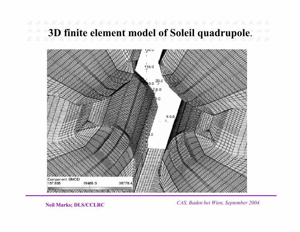
3D finite element model of Soleil quadrupole.

Neil Marks; DLS/CCLRC CAS, Baden bei Wien, September 2004
Magnet EndsIt is necessary to terminate the magnet in a controlled way:•to define the length (strength);•to prevent saturation in a sharp corner (see diagram);•to maintain length constant with x, y;•to prevent flux entering normal
to lamination (ac).
The end of the magnet is therefore'chamfered' to give increasing gap(or inscribed radius) and lower fields as the end is approached

Neil Marks; DLS/CCLRC CAS, Baden bei Wien, September 2004
Classical end solutionThe 'Rogowski' roll-off:Equation:
y = g/2 +(g/π) exp ((πx/g)-1);g/2 is dipole half gap;y = 0 is centre line of gap.
10-1-20
1
2
This profile provides the maximum rate of increase in gap with a monotonic decrease in flux density at the surface ie no saturation

Neil Marks; DLS/CCLRC CAS, Baden bei Wien, September 2004
Calculation of end field distributionCalculation of end effects in longitudinal plane using 2D codes,with correct end geometry (including coil), but 'idealised' return yoke:
+
-
This provides a reasonable estimate of the distribution in the third plane using a 2D code. BUT it is not as accurate as using a full 3D code.