Embed Size (px)
Citation preview

Controlling illumination to increaseinformation in a collection of images
Asla Medeiros e Sa

ii

Abstract
The solution of several problems inComputer Visionbenefits from analyzing col-lections of images, instead of a single image, of a scene that has variant and in-variant elements that give important additional clues to interpret scene structure.If the acquisition is done specially for some vision task, then acquisition parame-ters can be set up so as to simplify the interpretation task. In particular, changesin scene illumination can significantly increase information about scene structurein a collection of images.
In this work, the concept ofactive illumination, that is, controlled illuminationthat interferes on the scene at acquisition time, is explored to solve some Com-puter Vision tasks. For instance, a minimal structured light pattern is proposed tosolve stereo correspondence problem, while intensity modulation is used to help inforeground/background segmentation task as well as in image tone enhancement.
iii

iv ABSTRACT
Resumo
A solucao de varios problemas deVisao Computacionalpode se beneficiar daanalise de uma colecao de imagens, ao inves de utilizar umaunica imagem, deuma cena que possui elementos variaveis e invariantes capazes de fornecer dicasadicionais importantes para interpretar a estrutura de uma cena. Se a aquisicao dasimagens for feita especialmente para uma determinada tarefa, entao os parametrosde aquisicao podem ser escolhidos de forma a facilitar a interpretacao dos da-dos para a dada tarefa. Em particular, variacoes nas condicoes de iluminacao deuma cena podem aumentar significativamente a quantidade de informacao de umacolecao de imagens sobre a estrutura da cena.
Neste trabalho, o conceito deiluminacao ativa, isto e, iluminacao controladaque interfere na cena em tempo de aquisicao, e explorado para resolver algu-mas tarefas de Visao Computacional. Por exemplo, um padrao minimal de luzestruturadae proposto para a solucao do problema de correspondencia estereo;enquanto que a modulacao da intensidade da luze usada para auxiliar a tarefade segmentacao figura/fundo, bem como para melhorar a representacao tonal daimagem.
v

vi RESUMO
Acknowledgements
First of all I would like to thank Paulo Cezar Carvalho for the patience and con-stant participation in my academic career. Thanks to Luiz Velho for the enthusias-tic discussions. Thanks toMax-Planck Institut fur Informatikfor the opportunityto visit their Computer Graphics research group, and special thanks to MichaelGoesele for his visit toIMPA and the valuable comments and suggestions on mywork. Special thanks also to Marcelo Gattass and the support given byTecgraf.
Special thanks to Marcelo Bernardes who implemented the video (V4D) basedon the structured light coding scheme proposed in this thesis as well as the real-time active tone-enhancement video. Marcelo is also a co-author of the graph-cut segmentation application presented in Chapter 5. Thanks to Anselmo Mon-tenegro who actively participated in discussions and implementation of Chapter5. Thanks to Michele, the girl on the test images that patiently participated onour experiments. To myVisgraf colleagues, specially Victor Bogado, Robertode Beauclair, Adelailson Peixoto, Esdras Soares, Moacyr Alvim Horta, ViniciusMello and Serginho Krako. Special thanks also to Google.
Thanks to Patricia Gouvea and Simone Rodrigues for the opportunity to be atAtelie da Imagemlearning photography. Still concerning photography I also owemany thanks to Cesar Barreto, Frank Scanner and Otavio Schipper.
I would also like to thank my dear friends: Aubin, Re, Ronaldo, Lola, Aline,Paulo e Paula... and Candi. My Yoga instructors Marcio Oliveira, HorivaldoGomes, Tat Pinheiro, Mercedes Chavarria and to my Yoga colleagues. Rol, Jerome,Li, Marcio, Vitor e pai. E sobretudo ao Raina, nossa Clarice e nossa family.
vii

viii ACKNOWLEDGEMENTS
Contents
Abstract iii
Resumo v
Acknowledgements vii
1 Introduction 11.1 Problem Statement . . . . . . . . . . . . . . . . . . . . . . . . . 31.2 Chapters Overview . . . . . . . . . . . . . . . . . . . . . . . . . 41.3 Main Contributions . . . . . . . . . . . . . . . . . . . . . . . . . 6
2 Imaging Devices 72.1 Digital Image . . . . . . . . . . . . . . . . . . . . . . . . . . . . 7
2.1.1 Modeling Light and Color . . . . . . . . . . . . . . . . . 82.1.2 Measuring Light . . . . . . . . . . . . . . . . . . . . . . 9
2.2 Image Emitting Devices . . . . . . . . . . . . . . . . . . . . . . . 102.2.1 Light Sources . . . . . . . . . . . . . . . . . . . . . . . . 112.2.2 Digital Image Projectors . . . . . . . . . . . . . . . . . . 11
2.3 Scene Reflective Properties . . . . . . . . . . . . . . . . . . . . . 132.4 Imaging Capture Devices . . . . . . . . . . . . . . . . . . . . . . 14
2.4.1 Tonal Range and Tonal Resolution . . . . . . . . . . . . . 172.4.2 Color Reproduction . . . . . . . . . . . . . . . . . . . . . 202.4.3 Spatial resolution . . . . . . . . . . . . . . . . . . . . . . 212.4.4 Noise, Aberrations and Artifacts . . . . . . . . . . . . . . 22
3 Active Setup 253.1 Camera Calibration . . . . . . . . . . . . . . . . . . . . . . . . . 26
3.1.1 Intensity Response Function . . . . . . . . . . . . . . . . 27
ix
x CONTENTS
3.1.2 Spectral Calibration . . . . . . . . . . . . . . . . . . . . 323.2 Projector Calibration . . . . . . . . . . . . . . . . . . . . . . . . 33
3.2.1 Intensity Emitting Function . . . . . . . . . . . . . . . . 343.3 Calibration in Practice . . . . . . . . . . . . . . . . . . . . . . . 36
3.3.1 Camera Calibration . . . . . . . . . . . . . . . . . . . . . 363.3.2 Projector Calibration . . . . . . . . . . . . . . . . . . . . 39
4 Stereo Correspondence 434.1 Active Stereo . . . . . . . . . . . . . . . . . . . . . . . . . . . . 45
4.1.1 Coding Principles . . . . . . . . . . . . . . . . . . . . . . 474.1.2 Taxonomy . . . . . . . . . . . . . . . . . . . . . . . . . 50
4.2 Minimal Code Design . . . . . . . . . . . . . . . . . . . . . . . . 534.2.1 Minimal Robust Alphabet . . . . . . . . . . . . . . . . . 534.2.2 Codeword design - (6,2)-BCSL . . . . . . . . . . . . . . 55
4.3 Receiving and Cleaning the Transmitted Code . . . . . . . . . . . 584.3.1 Boundary Detection . . . . . . . . . . . . . . . . . . . . 584.3.2 Colors and Texture Recovery . . . . . . . . . . . . . . . . 60
4.4 Video Implementation . . . . . . . . . . . . . . . . . . . . . . . 62
5 Image Segmentation 655.1 Foreground - Background Segmentation . . . . . . . . . . . . . . 665.2 Active Segmentation . . . . . . . . . . . . . . . . . . . . . . . . 67
5.2.1 Active illumination with Graph-Cut Optimization . . . . . 685.3 The objective function . . . . . . . . . . . . . . . . . . . . . . . 69
5.3.1 Composing the cost functions . . . . . . . . . . . . . . . 705.4 Method and Results . . . . . . . . . . . . . . . . . . . . . . . . . 73
6 Tonal Range and Tonal Resolution 776.1 HDRI reconstruction: absolute tones . . . . . . . . . . . . . . . . 77
6.1.1 HDRI Acquisition . . . . . . . . . . . . . . . . . . . . . 786.1.2 HDRI Visualization . . . . . . . . . . . . . . . . . . . . . 796.1.3 HDRI Encoding . . . . . . . . . . . . . . . . . . . . . . 81
6.2 Partial reconstruction: relative tones . . . . . . . . . . . . . . . . 826.2.1 Active range-enhancement . . . . . . . . . . . . . . . . . 84
6.3 Real-time Tone-Enhanced Video . . . . . . . . . . . . . . . . . . 85
7 Conclusion 877.1 Future Work . . . . . . . . . . . . . . . . . . . . . . . . . . . . . 89
Chapter 1
Introduction
Computer Graphics(CG) studies methods for creating and structuring graphicsdata as well as methods for turning these data into images.Computer Vision(CV)studies the inverse problem: given an input image or a collection of input images,obtain information about the world and turn it into graphics data. CG problems areusually stated as direct problems while in CV they are naturally stated as inverseproblems. There are several ways to control input data acquisition acquisition inorder to ease CV tasks. The knowledge and control on how images are acquiredin many cases determines the approaches to be used to solve the CV problem athand.
A single image of a scene can suffer from lack of information to infer worldstructure. Many CV systems benefit from analyzing a collection of images to in-crease information about the world and obtain important clues about scene struc-ture, such as object movement, changes in camera view point, changes in shading,etc. Also CG image processing can benefit from collection of images to synthe-size new images, as was widely explored in [ADA∗04]. By using collections ofimages it is possible to identify invariant elements in the set of images; the detec-tion of varying elements together with the knowledge of what caused the variation(camera movement, object movement, changes in lighting, changes in focus, etc.)is helpful to analyze data.
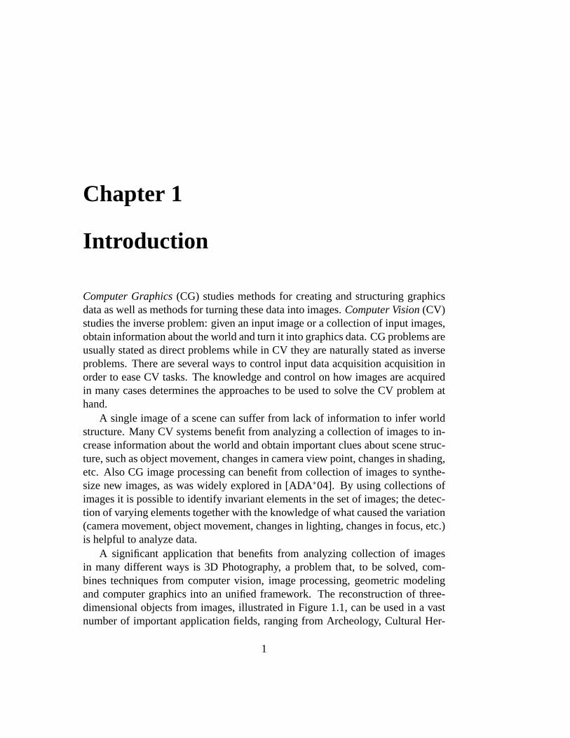
A significant application that benefits from analyzing collection of imagesin many different ways is 3D Photography, a problem that, to be solved, com-bines techniques from computer vision, image processing, geometric modelingand computer graphics into an unified framework. The reconstruction of three-dimensional objects from images, illustrated in Figure 1.1, can be used in a vastnumber of important application fields, ranging from Archeology, Cultural Her-
1
2 CHAPTER 1. INTRODUCTION
itage, Art and Education, to Electronic Commerce and Industrial Design.
The development of commodity hardware and consumer electronics makesit possible to build low-cost acquisition systems that are increasingly effective.Some applications demand precision in the acquisition of a scene’s radiance prop-erties that up-to-date off-the-shelf sensors can’t provide. For instance, to visualizean object with illumination conditions different from the illumination of the ambi-ent where the object was captured, the object capture has to satisfy some requisitesthat are beyond most sensors capabilities [Len03, Goe04].
In particular,active illuminationis a powerful tool to increase image infor-mation at acquisition time. By active illumination we mean a controllable lightsource that can be modulated or moved in order to augment scene structure in-formation in a sequence of images, either by controlling shading or by directlyprojecting information onto the scene. Examples of active illumination in actionare shown in Figures 1.1, 1.2 and 1.3.
(a) (b) (c)
Figure 1.1: Images (a) and (b) are images acquired by a photographic digitalcamera that observes the scene illuminated by projected coded patterns. Stripeboundaries (c) and depth at boundary points can be recovered using structuredlight principles.
This thesis focuses on controlling illumination to increase image informationat acquisition time, that is, to acquire additional information not present in a singleshot, by changing scene illumination. By exploring the illumination control wego through different areas of recent research inComputer Vision, like shape ac-quisition from structured light, active image segmentation and tone enhancement.
1.1. PROBLEM STATEMENT 3
1.1 Problem Statement
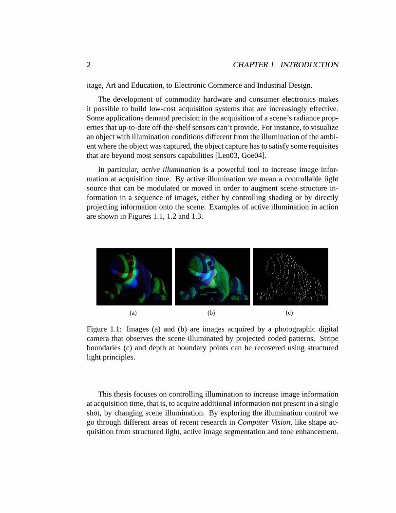
Digital photographic images are projections of a real scene through a lens sys-tem onto a photosensitive sensor. At acquisition time, image information can beincreased by marking the scene with controlled illumination, this is the principleof active illumination. The standard active illumination setup uses a pair cam-era/projector where the camera produces images of a scene illuminated by theprojector in a desired fashion.
(a) (b) (c)
Figure 1.2: Images (a) and (b) have been differently illuminated by varying thecamera flash intensity between shots, (c) is the difference thresholded image thatcan be used to segment objects from non-illuminated backgrounds.
We are particularly interested in exploring the potential of camera/projectorpairs. A digital camera can be seen as a non-linear photosensitive black box thatacquires digital images, while a projector is another non-linear black box thatemits digital images. Their non-linear behavior is a consequence of several tech-nical issues ranging from techniques limitations to market demands to producebeautiful images.
In order for these black boxes to become measurement tools it is mandatoryto characterize their non-linear behavior, that is, to perform a calibration step. Insome cases, absolute color calibration relating devices to global world referencesis needed. However, in our case, we will be concerned with the relative cali-bration of a camera/projector pair, since we only want to guarantee a consistentcommunication between them.
We explore scene illumination to extract more information of a given scene.The digital projector is our standard active light source. It can project struc-tured light onto the scene in order to recover geometric information (Figure 1.1),and modulate light intensity to help solving background/foreground segmentation(Figure 1.2), or improve tonal information (Figure 1.3).
4 CHAPTER 1. INTRODUCTION
(a) (b) (c)
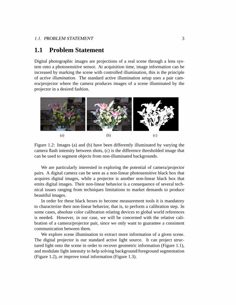
Figure 1.3: Images (a) and (b) are two subsequent video input fields. In thisexperiment a video camera synchronized with a digital projector acquire imageswith modulated projected light intensity. In (c) it is shown the tonal-enhancedforeground produced from processing together both (a) and (b) frames.
1.2 Chapters Overview
The main reasoning that guides this work is active illumination. Active illumi-nation will be used in different applications with different setups ranging fromfine tunned setups of lab environments to cheap home-made setups. Traditionallyactive illumination is used in 3D photography for depth acquisition. In this workactive illumination is used also to solve other problems in Computer Vision. Themain overall concepts found in literature that will be useful to the entire work areintroduced in Chapter 2.
Photometric calibration enhance the setup performance, and it is mandatoryif the setup is to be used as a measurement tool. Calibration will be discussed inChapter 3, where a basic setup is calibrated. The difference between projected andobserved colors is clearly observed in calibration results as well as the non-linearprojector intensity behavior. After setup description and calibration we turn intoapplications.
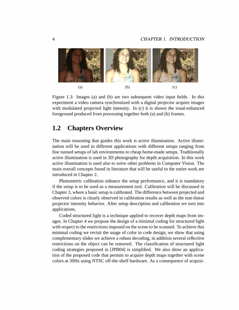
Coded structured light is a technique applied to recover depth maps from im-ages. In Chapter 4 we propose the design of a minimal coding for structured lightwith respect to the restrictions imposed on the scene to be scanned. To achieve thisminimal coding we revisit the usage of color in code design, we show that usingcomplementary slides we achieve a robust decoding, in addition several reflectiverestrictions on the object can be removed. The classification of structured lightcoding strategies proposed in [JPB04] is simplified. We also show an applica-tion of the proposed code that permits to acquire depth maps together with scenecolors at 30Hz using NTSC off-the-shelf hardware. As a consequence of acquisi-
1.2. CHAPTERS OVERVIEW 5
tion of geometry and texture from the same data the texture-geometry registrationproblem is avoided.
In Chapter 5 the problem of foreground segmentation using active illuminationand graph-cut optimization is discussed. The key idea is that light source position-ing and intensity modulation can be designed to affect objects that are closer to thecamera and let the background unchanged. Following this reasoning, a scene is litwith two different intensities of a controllable light source that we call segmen-tation light source. By capturing a pair of images with such illumination, we areable to produce a mask that distinguishes between foreground objects and scenebackground. The initial segmentation is optimized by graph-cut optimization.
The quality of the masks produced by the method is, in general, quite good.Some difficult cases may arise when the objects are highly specular, translucent orhave very low reflectance. Because of its characteristics, the camera parameterssettings chosen according to the situation in hand can strongly influence on thequality of the output mask.
In Chapter 6 the concept of relative tone values will be introduced. The factthat relative tones can be recovered, by varying illumination intensity, withoutknowledge about the camera response function is presented. In our approach, weilluminate the scene with an uncalibrated projector and capture two images of thescene under different illumination conditions. The output of our system is a seg-mentation mask, together with an image with enhanced tonal information for theforeground pixels. The segmentation and the visualization algorithms are imple-mented in real-time, and can be used to produce range-enhanced video sequences.
The system is implemented using two different setups. The first uses the sameacquisition device built for the stereo correspondence application and is composedof a NTSC camera synchronized with a DLP projector. The second is a homemade cheap version of the system that uses a web cam synchronized with a CRTmonitor playing the role of the light source.
Although our implementation has been done in real time for video, the sameidea could be used in digital cameras by programming flashes. There are manyrecent works [PAH∗04, ED04] that explore the use of programmable flash to en-hance image quality, but they do not introduce tone-enhancement concepts.
Conclusions and future work will be discussed in Chapter 7.

6 CHAPTER 1. INTRODUCTION
1.3 Main Contributions
We list below the main original contribution of this thesis, some of which havealready been published:
• Relative photometric calibration of an active pair camera-projector.
• Proposal of (b,s)-BCSL (Figure 1.1), a minimal structured light coding foractive stereo correspondence [SCV02, VSVC05].
• Light intensity modulation for active segmentation using graph-cuts (Figure1.2).
• The concept of relative tones as a tool to tone enhance LDR images withoutHDR recovery (Figure 1.3) [SVCV05].
Chapter 2
Imaging Devices
Image capture devices measure the flux of photons that were emitted from a lightsource and interacted with the observed scene. Tasks in Computer Vision areheavily dependent on such devices. For that reason, we are interested in how lightsources and the scene behave with respect to visible energy flux that reaches theimaging device. In this chapter we review the most relevant characteristics oflight sources, imaging emitters, scene reflectivity properties and imaging capturedevices.
2.1 Digital Image
The basic elements of a digital image are the pixel coordinates and the color in-formation at each pixel. Pixel coordinates are related to image spatial resolutionwhile color resolution is determined by how color information is captured andstored. If the instrument used to capture the image is a camera, we obtain a pho-tographic image, that is, a projection of a real scene that passed through a lenssystem to reach a photosensitive sensor. A photographic image can be modeledas a functionf : U ⊆ R2 → C representing light intensity information at eachmeasurement pointp ∈ U . The measured intensity values depend upon physicalproperties of the scene being viewed and on the light sources distribution as wellas on photosensitive sensor characteristics.
In order to digitize the image signal that reaches the sensor asamplingopera-tion is carried on.Samplingis the task of converting the continuous incoming lightinto a discrete representation. The scene is sampled at a finite number of points,where the intensity functionf takes on values in a discrete subset of the color
7
8 CHAPTER 2. IMAGING DEVICES
spaceC. Color space discretization is also calledquantization. Thecolor resolu-tion of an image is usually expressed by the number of bits used to store the colorinformation. Image sensors are physical implementations of signal discretizationoperators [GV97].
To visualize the image, areconstructionoperation recovers the original signalfrom samples. Ideally, the reconstruction operation should recover the originalsignal from the discretized information; however, the result of reconstruction fre-quently is only an approximation of the original signal. Imaging devices, suchas digital projectors, monitors and printers, reconstruct the discrete image to beviewed by the observer. It should be noted that the observer’s visual system alsoplays a role in the reconstruction process.
2.1.1 Modeling Light and Color
The physics of light is usually described by two different models,Quantum Opticsdescribes photons behavior, andWave Optics, models light as an eletromagnecticwave [Goe04]. The most relevant light characteristics that will be useful to us arewell described by the eletromagnectic model;Geometric Opticsis an approxima-tion of wave optics. We will adopt the eletromagnectic approach and geometricoptics when it is convenient.
Light sources radiate photons within a range of wavelengths. The energy ofeach photon is related to its wave frequency by thePlanck’sconstanth, that is,E = hf . Once the frequency is determined, the associated wavelengthλ is alsoknown through the relationc = λf . The emitted light can be characterized byits spectral distributionthat associates to each wavelength a measurement of theassociated radiant energy, as illustred in Figure 2.1(a). A source of radiation thatemits photons all with the same wavelength is calledmonochromatic[GV97].
A photosensitive sensor is characterized by itsspectral response functions(λ).If a sensor is exposed to light with spectral distributionC(λ), the resulting men-surable value is given by
w =∫
λC(λ)s(λ)dλ
The human eye has three types of photosensors with specific spectral responsecurves. Light sensors and emitters try to mimic the original signal with respect tohuman perception. The standard solution adopted by industry is to use red, greenand blue filters asprimary colors to sample and reconstruct the emitted light,illustred in Figure 2.1(b). The interval of wavelengths perceived by the humaneye is between the range of 380 nm to 780 nm, known as thevisible spectrum.
2.1. DIGITAL IMAGE 9
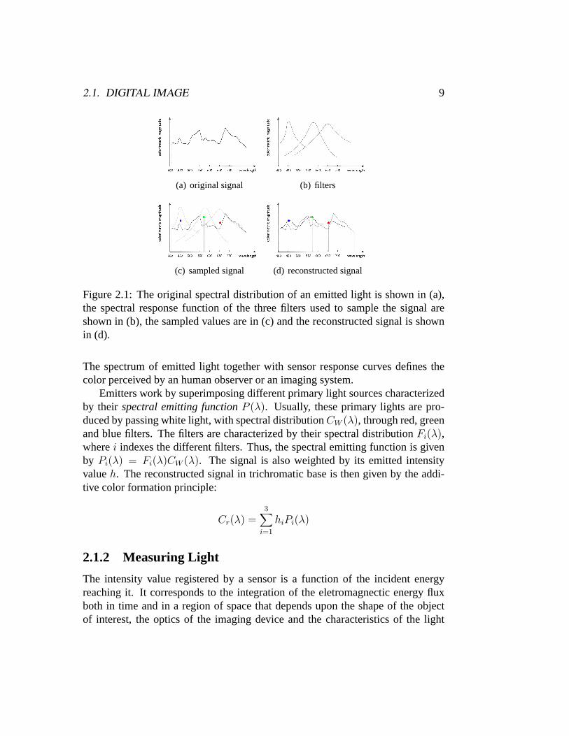
(a) original signal (b) filters
(c) sampled signal (d) reconstructed signal
Figure 2.1: The original spectral distribution of an emitted light is shown in (a),the spectral response function of the three filters used to sample the signal areshown in (b), the sampled values are in (c) and the reconstructed signal is shownin (d).
The spectrum of emitted light together with sensor response curves defines thecolor perceived by an human observer or an imaging system.
Emitters work by superimposing different primary light sources characterizedby their spectral emitting functionP (λ). Usually, these primary lights are pro-duced by passing white light, with spectral distributionCW (λ), through red, greenand blue filters. The filters are characterized by their spectral distributionFi(λ),wherei indexes the different filters. Thus, the spectral emitting function is givenby Pi(λ) = Fi(λ)CW (λ). The signal is also weighted by its emitted intensityvalueh. The reconstructed signal in trichromatic base is then given by the addi-tive color formation principle:
Cr(λ) =3∑
i=1
hiPi(λ)
2.1.2 Measuring Light
The intensity value registered by a sensor is a function of the incident energyreaching it. It corresponds to the integration of the eletromagnectic energy fluxboth in time and in a region of space that depends upon the shape of the objectof interest, the optics of the imaging device and the characteristics of the light
10 CHAPTER 2. IMAGING DEVICES
sources.Radiometryis the field that study electromagnetic energy flux measurements.
The human visual system is only responsive to energy in a certain range of theelectromagnetic spectrum, that is thevisible spectrum. If the wavelength is inthe visible spectrum, the radiometric quantities are also described inphotometricterms. Photometric terms are simply radiometric terms weighted by the humanvisual system spectral response function [Gla94].
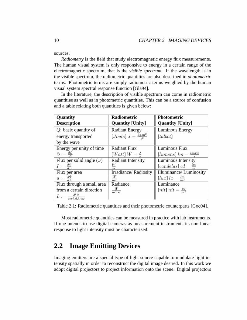
In the literature, the description of visible spectrum can come in radiometricquantities as well as in photometric quantities. This can be a source of confusionand a table relating both quantities is given below:
Quantity Radiometric PhotometricDescription Quantity [Unity] Quantity [Unity]Q: basic quantity of Radiant Energy Luminous Energyenergy transported [Joule] J = kg.m2
s2 [talbot]by the waveEnergy per unity of time Radiant Flux Luminous FluxΦ := dQ
dt[Watt] W = J
s[lumens] lm = talbot
s
Flux per solid angle (ω) Radiant Intensity Luminous IntensityI := dΦ
dωWsr
[candelas] cd = lmsr
Flux per area Irradiance/ Radiosity Illuminance/ Luminosityu := dΦ
dAWm2 [lux] lx = lm
m2
Flux through a small area Radiance Luminancefrom a certain direction W
m2.sr[nit] nit = cd
m2
L := d2Φcosθ.dA.dω
Table 2.1: Radiometric quantities and their photometric counterparts [Goe04].
Most radiometric quantities can be measured in practice with lab instruments.If one intends to use digital cameras as measurement instruments its non-linearresponse to light intensity must be characterized.
2.2 Image Emitting Devices
Imaging emitters are a special type of light source capable to modulate light in-tensity spatially in order to reconstruct the digital image desired. In this work weadopt digital projectors to project information onto the scene. Digital projectors
2.2. IMAGE EMITTING DEVICES 11
will be modeled with the intention to understand its behavior and their technologicpeculiarities will be observed.
2.2.1 Light Sources
Usual light sources contain various elements that shape its radiation pattern; dif-fusors, mirrors and lenses can be used to characterize, change direction and focusthe emitted light. According to their emission, light sources can be classified intopoint and area light sources.
A point light sourceis characterized by the fact that all light is emitted froma single point in space. For anuniform point light sourcelight is emitted equallyin all directions. Aspot lightis a uniform point light source that emits light onlywithin a cone of directions. Fortextured point light sourcesthe intensity can varyfreely with the emission direction. This model is useful in rendering but rare inreal world. Finally, anarea light sourcein contrast to point light source emit lightfrom a region in space and is responsible for the presence ofsoft shadowsin thescene consisting ofumbraandpenumbraregions [Goe04].
2.2.2 Digital Image Projectors
In the rendering context image projectors can be conveniently modeled as a tex-tured spot light source. This model does not take into account the effects resultantof the presence of projector lenses. In this work, images of a real scene withprojected patterns will be observed by the camera, so we need a more completemodel, capable of a better description of real digital projectors behavior.
Real digital projectors usually are composed of a single lamp whose rays passthrough an array of light intensity modulators in order to form an image. Afterthat, light passes through a lens system to be focused at some plane of focus. If weconsider that, after being modulated, each point in space is an independent spotlight source, then a reasonable model of a general digital projector is to consideran array of spot light sources that passes through a single lens system. Each spotlight source from the projector array will be referred as aprojector pixel. With thismodel it is possible to simulate the plane of focus and the out-of-focus regions, aswell as neighborhood spot light interaction.
The projector lamp is described by its spectral distributionCl(λ). For eachprojector pixel, a given digital intensity valueρ is to be projected. The actualemitted intensity value is given by the projectorcharacteristic emitting functionh(ρ), dependent on the projector technology and other factors. To produce colored
12 CHAPTER 2. IMAGING DEVICES
images, color filters with spectral distributionFi(λ) are used, wherei indexescolor channels. The resultantspectral emitting functionper channel isPi(λ) =Fi(λ)Cl(λ). The actual emitted signal at each channel of a projector pixel is then:
Ci(λ, ρ) = h(ρ)Pi(λ)
Below, the two most common digital projectors technologies are described inmore detail.
LCD vs. DLP technology
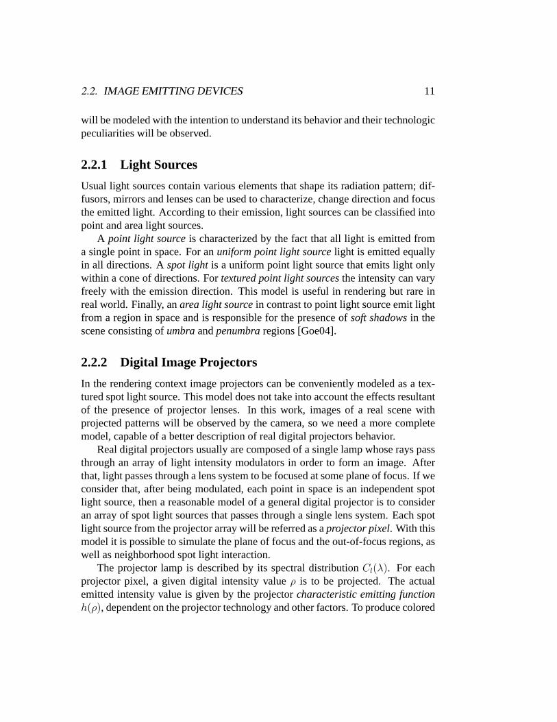
LCD (Liquid Crystal Display) projectors, illustrated in Figure 2.2 (a), usuallycontain three separate LCD glass panels, one each for red, green, and blue com-ponents of the image signal. As light passes through the LCD panels, individualpixels can be opened to allow light to pass or closed to block the light. This ac-tivity modulates the light and produces the image that is projected onto the screen[Powa].
(a) (b)
Figure 2.2: A LCD projector technology (a) compared to a DLP technology (b).
The DLP (Digital Light Processing) chip, Figure 2.2 (b), is a reflective surfacemade up of one tiny mirror for each pixel. Light from the projector’s lamp isdirected onto the surface of the DLP chip. The mirrors wobble back and forth,directing light either into the lens path to turn the pixel on, or away from the lenspath to turn it off.
In DLP projectors, usually there is only one DLP chip (some have three chips,one per channel); in order to define color, there is a color wheel that filters incom-ing light. This wheel spins between the lamp and the DLP chip and alternates the
2.3. SCENE REFLECTIVE PROPERTIES 13
color of the light hitting the chip from red to green to blue. The mirrors tilt awayfrom or into the lens path based upon how much of each color is required for eachpixel. This activity modulates the light and produces the image that is projectedonto the screen [Powa].
The use of a spinning color wheel to modulate the image has the potential toproduce a unique visible artifact on the screen referred as the ”rainbow effect”,which is simply colors separating out in distinct red, green, and blue. Basically, atany given instant in time, the image on the screen is either red, or green, or blue.The technology relies upon human eyes not being able to detect the rapid colorchanges, what is not always true, especially with respect to frame rate variations.
Consumers can decide on the preferred technology by analyzing its effects inpractice. LCD usually delivers a somewhat sharper image than DLP at any givenresolution. LCD projectors produce a visible pixelation, clearly reduced on DLPs.DLP technology can produce higher contrast video with deeper black levels thanwhat is usually obtained with an LCD projector. Leading-edge LCD projectorsare rated at 1000:1 contrast. Meanwhile, the latest DLP products are rated as highas 3000:1 [Powa].
There are also other technologies used in digital projectors, but DLP and LCDare the most commonly available and cheaper. We will restrict our discussion tothem.
2.3 Scene Reflective Properties
The interaction of light and matter is a complex physical process. For graphicspurposes, materials can be characterized by their reflective properties. When lightreaches an object surface it is partially reflected back to the ambient. The surfacereflectanceis the fraction of the incident flux that is reflected, and it is a functionof wavelength, position, time, incident and exitant directions and polarization. Inalmost all physical materials, surface scattering is linear, that is, energy arrivingfrom each direction contributes independently to the reflection.
By assuming that some materials won’t be present in the scene of interest someuseful simplifications can be made to characterize the reflective function. Polar-ization can be reasonably ignored. Different wavelengths can be assumed to bedecoupled, that is, the energy at wavelengthλ1 is independent of the energy atλ2.This excludesfluorescent materials, where energy is absorbed at one wavelengthand reradiated at another. It can also be assumed that there is no time-dependentbehavior, what excludesphosphorescent materials. Complex phenomena such as
14 CHAPTER 2. IMAGING DEVICES
subsurface scattering, where light is reflected also inside the surface generatingmultiple scattering events per incident ray, will be also ignored. Considering theabove simplifications, the reflectance becomes, to each wavelength, a function ofposition and incident and exitant directions.
Without subsurface light transport, all light arriving at an object’s surface iseither reflected or absorbed at the incidence point. This behavior is usually de-scribed by thebidirectional reflectance distribution function(BRDF) that incor-porates the simplifications above. The BRDF functionfλ(p, ωi, ωo) is the ratio ofthe reflected radiance leaving the surface at a pointp in directionωo to the irradi-ance arriving at the same pointp from a directionωi. Other models incorporatethe behaviors not described by BRDFs [Gla94, Goe04].
Further simplifications are much more restrictive in terms of real objects. Forinstance, reflectance ofhomogeneous materialsis independent of position; forisotropic materialsincoming and outgoing directions can be rotated around thesurface normal without change, and fordiffuse materialsreflectance is indepen-dent of direction. Perfectly homogeneous materials as well as perfectly diffusematerials rarely occurs in real world.
If one have in hand the BRDF of the desired material, the rendering of a vir-tual object with such aspect is a direct problem treated in Computer Graphics. Theacquisition of BRDFs of given real materials is measured in practice with lab in-struments. Recently, digital cameras have been used as such instruments [Len03],and the problem is stated as a typical inverse problem heavily dependent on thequality of data acquisition.
Note that if scene, camera and light source are static, then for each camerapixel the surface position and incoming and outgoing directions are well defined.In this case additive behavior of light is preserved by surface reflectance; thisproperty will be useful in Chapter 4.
2.4 Imaging Capture Devices
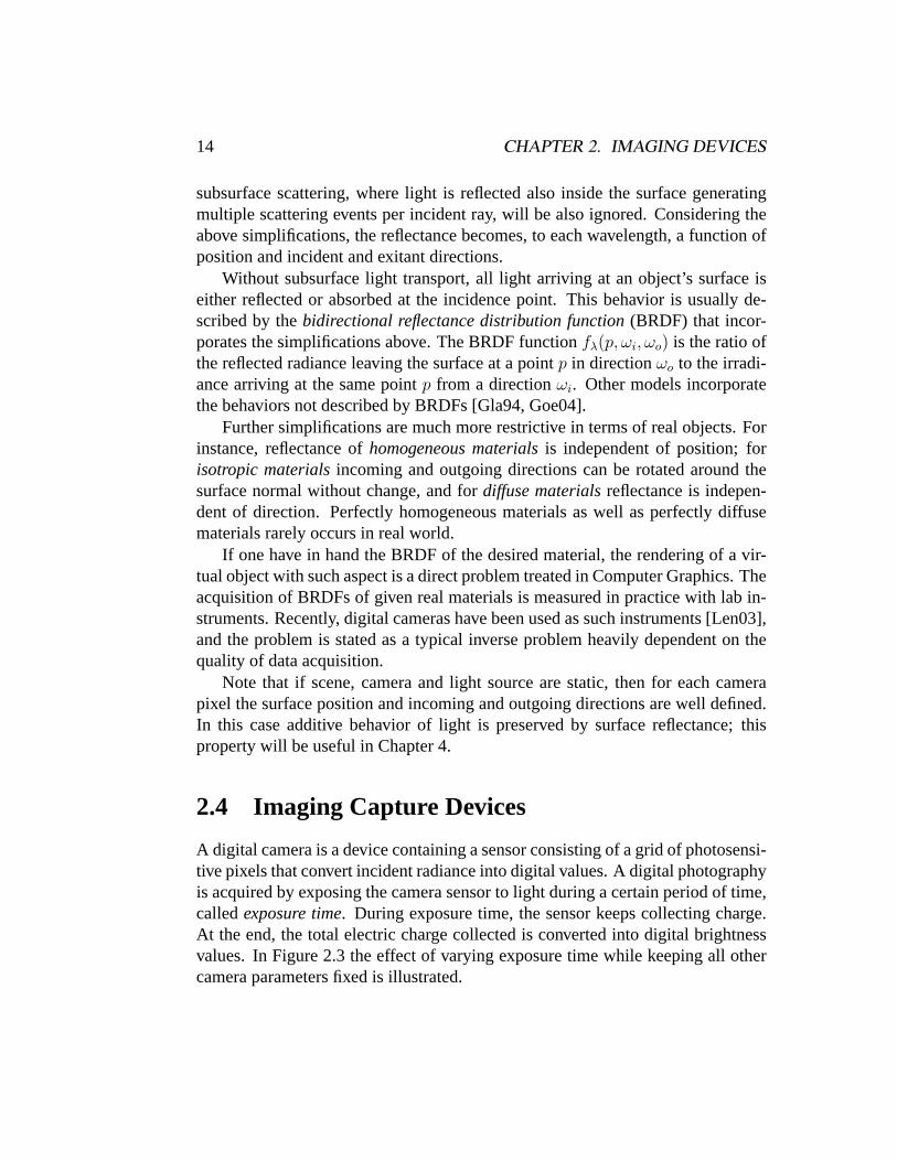
A digital camera is a device containing a sensor consisting of a grid of photosensi-tive pixels that convert incident radiance into digital values. A digital photographyis acquired by exposing the camera sensor to light during a certain period of time,calledexposure time. During exposure time, the sensor keeps collecting charge.At the end, the total electric charge collected is converted into digital brightnessvalues. In Figure 2.3 the effect of varying exposure time while keeping all othercamera parameters fixed is illustrated.
2.4. IMAGING CAPTURE DEVICES 15
(a) overexposed sky (b) underexposed hill
Figure 2.3: This images illustrate the resultant acquired images when exposuretime is changed. In (a) the sensor has been exposed longer than in (b).
The fundamental information stored in a digital image is the pixelexposure,that is, the integral of the incident radiance on the exposure time. A reasonableassumption is that incident radiance is constant during exposure time, speciallywhen small exposure times are used. Thus exposure is given by the product ofincident radiance by total exposure time. The incident radiance valuewij is afunction of the scene’s radiance, optical parameters of the system and the anglebetween the light ray and system’s optical axis. The most obvious way to controlexposure is by varying exposure time, that is, by varying the total time that the sen-sor keeps collecting photons; but other camera parameters can also be controlledto alter exposure in different ways:
• controlling lens aperture;
• changing film/sensor sensitivity (ISO);
• using neutral density filters;
• modulating intensity of light source;
To vary time (as illustred in Figure 2.3) and lens aperture is easy and all pro-fessional and semi-professional cameras have these facilities. The disadvantagesare related to limitations in applications since long exposures can produce mo-tion blur while lens aperture affects the depth of focus, which can be a problem ifthe scene has many planes of interest. Film and sensor sensitivity can be alteredbut the level of noise and graininess are also affected. Density filters are commonphotographic accessories but its usage depends on an implementation in hardware,
16 CHAPTER 2. IMAGING DEVICES
or to be manually changed, which may not be practical. The use of controllablelight source is tricky since intensity change depends on the distance of objects tothe light source, that is, fails to change constantly on the scene and, in addition,produces shadows.
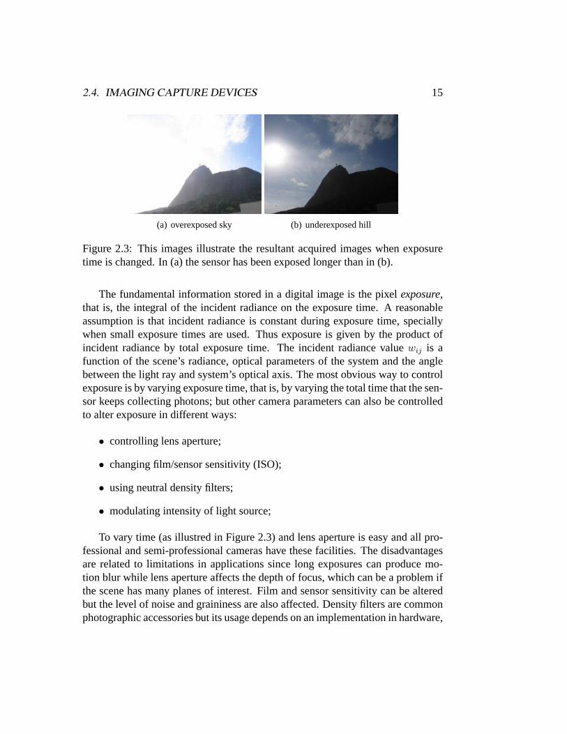
The photographic industry has been studying acquisition, storage and visu-alization of images for chemical emulsions since the beginning of the history ofphotography. Many concepts concerning image quality and accuracy were estab-lished since then [Ada80, Ada81, Ada83]. Technical information about photo-graphic material is available for reference in data sheets provided by manufactur-ers. The standard information provided is storage, processing and reproductioninformation, as well as its technical curves, shown in Figure 2.4.
Figure 2.4: FujiChrome Provia 400F Professional [RHP III] data sheet, from Fu-jiFilm.
2.4. IMAGING CAPTURE DEVICES 17
Film technical curves guide the characterization of emulsions and are the tech-nical base to chose an emulsion adequate for each scene and illumination situa-tion. To characterize emulsion light intensity response, the useful curve is thecharacteristic response curve. Spectral response curvesconsiders problems di-rectly related to color reproduction. TheMTF curvedescribe the spatial frequencyresolution power of the sensible area.
The classical characterization of emulsions can also guide the study of digi-tal sensors, although this information is usually not provided by digital sensorsmanufacturers. We turn now to the understanding of their role in digital imageformation.
2.4.1 Tonal Range and Tonal Resolution
Considering light intensity, the behavior of an imaging sensor is described by itscharacteristic response functionf . The distinct values registered by the sensor arethe imagetones.
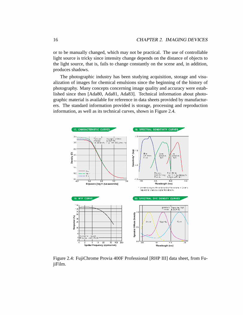
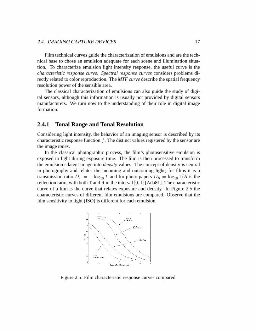
In the classical photographic process, the film’s photosensitive emulsion isexposed to light during exposure time. The film is then processed to transformthe emulsion’s latent image intodensityvalues. The concept of density is centralin photography and relates the incoming and outcoming light; for films it is atransmission ratioDT = − log10 T and for photo papersDR = log10 1/R is thereflection ratio, with both T and R in the interval[0, 1] [Ada81]. The characteristiccurve of a film is the curve that relates exposure and density. In Figure 2.5 thecharacteristic curves of different film emulsions are compared. Observe that thefilm sensitivity to light (ISO) is different for each emulsion.
Figure 2.5: Film characteristic response curves compared.
18 CHAPTER 2. IMAGING DEVICES
In digital photography, the film emulsions are replaced by photosensitive sen-sors. The sensor behavior depends on its technology. Usually the stored electricalcharge is highly linearly proportional to radiance values. In this case, if the sensoris capable to store a total number ofd electrons, then the maximum number ofdistinct digital brightness values, that is, itstonal resolution, will potentially beequal tod. In practice, the digitization process influences on final image tonalresolution. Another important concept is that oftonal range, that is the differencebetween the maximum and the minimum exposure values registered by the sensor.
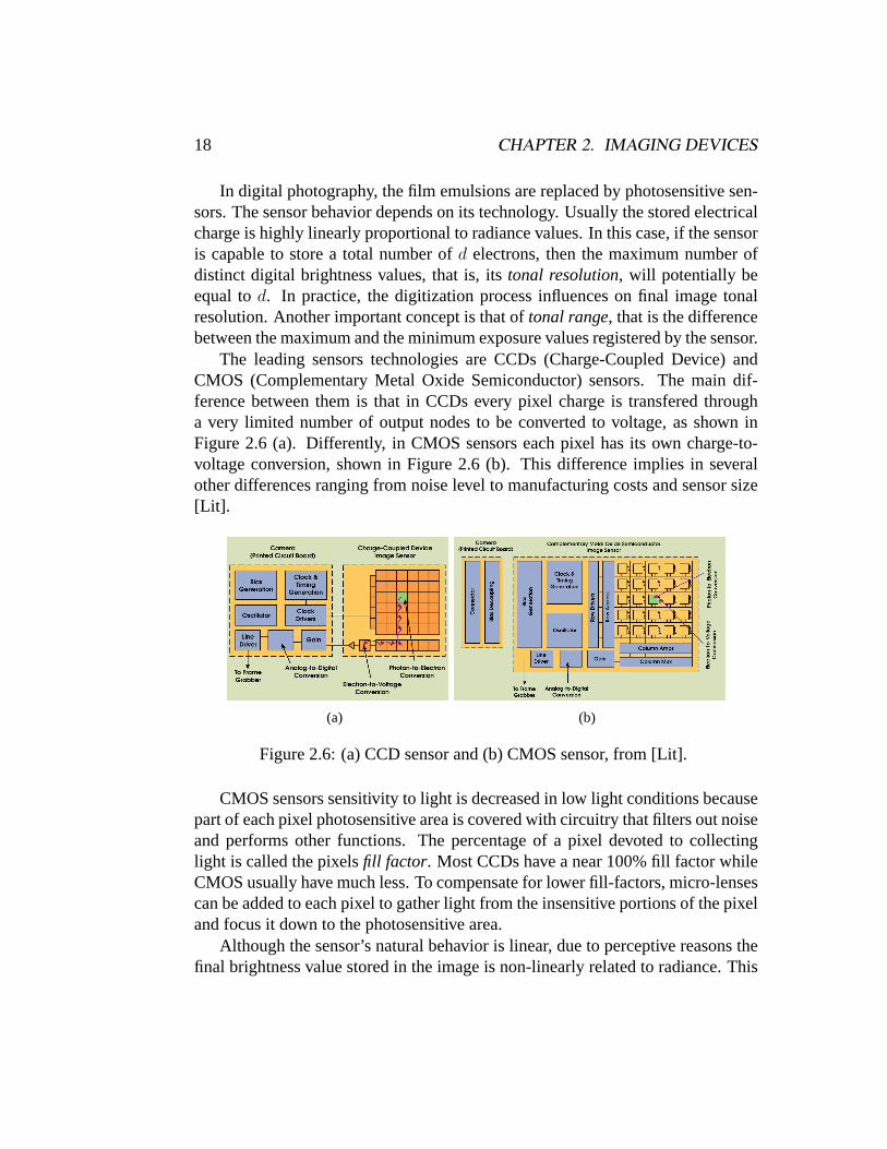
The leading sensors technologies are CCDs (Charge-Coupled Device) andCMOS (Complementary Metal Oxide Semiconductor) sensors. The main dif-ference between them is that in CCDs every pixel charge is transfered througha very limited number of output nodes to be converted to voltage, as shown inFigure 2.6 (a). Differently, in CMOS sensors each pixel has its own charge-to-voltage conversion, shown in Figure 2.6 (b). This difference implies in severalother differences ranging from noise level to manufacturing costs and sensor size[Lit].
(a) (b)
Figure 2.6: (a) CCD sensor and (b) CMOS sensor, from [Lit].
CMOS sensors sensitivity to light is decreased in low light conditions becausepart of each pixel photosensitive area is covered with circuitry that filters out noiseand performs other functions. The percentage of a pixel devoted to collectinglight is called the pixelsfill factor. Most CCDs have a near 100% fill factor whileCMOS usually have much less. To compensate for lower fill-factors, micro-lensescan be added to each pixel to gather light from the insensitive portions of the pixeland focus it down to the photosensitive area.
Although the sensor’s natural behavior is linear, due to perceptive reasons thefinal brightness value stored in the image is non-linearly related to radiance. This
2.4. IMAGING CAPTURE DEVICES 19
non-linear behavior is characterized by the camera response curve. Only somescientific cameras keep the sensor natural linear behavior to produce the final im-age.
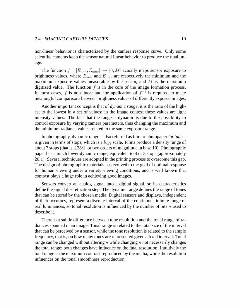
The functionf : [Emin, Emax] → [0, M ] actually maps sensor exposure tobrightness values, whereEmin andEmax are respectively the minimum and themaximum exposure values measurable by the sensor, andM is the maximumdigitized value. The functionf is in the core of the image formation process.In most cases,f is non-linear and the application off−1 is required to makemeaningful comparisons between brightness values of differently exposed images.
Another important concept is that ofdynamic range, it is the ratio of the high-est to the lowest in a set of values; in the image context these values are lightintensity values. The fact that the range is dynamic is due to the possibility tocontrol exposure by varying camera parameters, thus changing the maximum andthe minimum radiance values related to the same exposure range.
In photography, dynamic range – also referred as film or photopaperlatitude–is given in terms of stops, which is alog2 scale. Films produce a density range ofabout 7 stops (that is, 128:1, or two orders of magnitude in base 10). Photographicpaper has a much lower dynamic range, equivalent to 4 or 5 stops (approximately20:1). Several techniques are adopted in the printing process to overcome this gap.The design of photographic materials has evolved to the goal of optimal responsefor human viewing under a variety viewing conditions, and is well known thatcontrast plays a huge role in achieving good images.
Sensors convert an analog signal into a digital signal, so its characteristicsdefine the signal discretization step. The dynamic range defines the range of tonesthat can be stored by the chosen media. Digital sensors and displays, independentof their accuracy, represent a discrete interval of the continuous infinite range ofreal luminances, so tonal resolution is influenced by the number of bitsn used todescribe it.
There is a subtle difference between tone resolution and the tonal range of ra-diances spanned in an image. Tonal range is related to the total size of the intervalthat can be perceived by a sensor, while the tone resolution is related to the samplefrequency, that is, on how many tones are represented given a fixed interval. Tonalrange can be changed without alteringn while changingn not necessarily changesthe total range; both changes have influence on the final resolution. Intuitively thetotal range is the maximum contrast reproduced by the media, while the resolutioninfluences on the tonal smoothness reproduction.
20 CHAPTER 2. IMAGING DEVICES
2.4.2 Color Reproduction
As mentioned before, light sensors and emitters try to mimic the scene’s lightsignal concerning human perception; it is the human perception that is importantconcerning colors reproduction. Inspired on the trichromatic base of the humaneye, the standard solution adopted by industry is to use red, green and blue filters,referred as RGB base, to sample the input light signal and also to reproduce thesignal using light based image emitters. Printers work on a different principle, adiscussion about them is out of the scope of this work.
Photographic color films usually have three layers of emulsion, each with adifferent spectral curve, sensitive to red, green and blue light respectively. TheRGB spectral response of the film is characterized by spectral sensitivity and spec-tral dye density curves (see Figure 2.4).
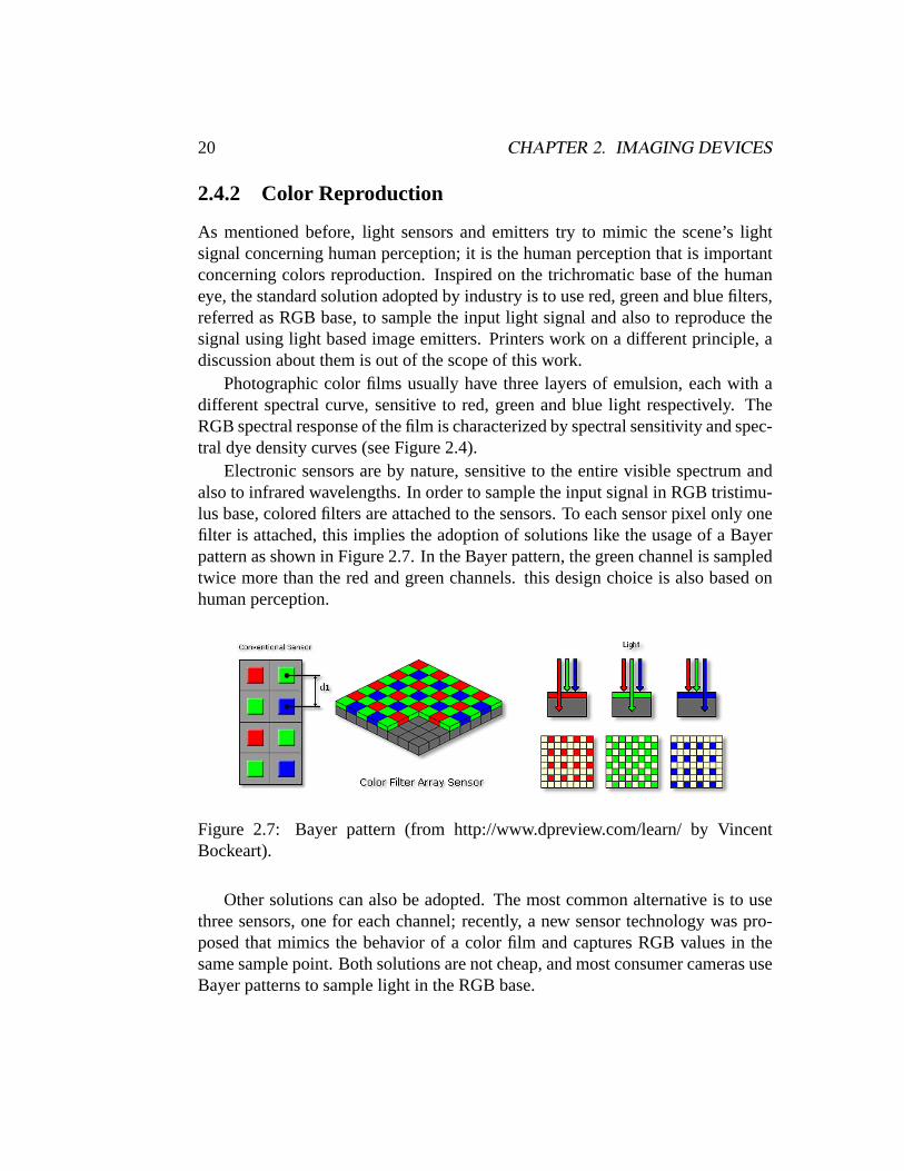
Electronic sensors are by nature, sensitive to the entire visible spectrum andalso to infrared wavelengths. In order to sample the input signal in RGB tristimu-lus base, colored filters are attached to the sensors. To each sensor pixel only onefilter is attached, this implies the adoption of solutions like the usage of a Bayerpattern as shown in Figure 2.7. In the Bayer pattern, the green channel is sampledtwice more than the red and green channels. this design choice is also based onhuman perception.
Figure 2.7: Bayer pattern (from http://www.dpreview.com/learn/ by VincentBockeart).
Other solutions can also be adopted. The most common alternative is to usethree sensors, one for each channel; recently, a new sensor technology was pro-posed that mimics the behavior of a color film and captures RGB values in thesame sample point. Both solutions are not cheap, and most consumer cameras useBayer patterns to sample light in the RGB base.
2.4. IMAGING CAPTURE DEVICES 21
2.4.3 Spatial resolution
The total size of the sensor, the size of an individual pixel and their spatial dis-tribution determine the image spatial resolution and the resolution power of thesensor. The spatial resolution power is related to the image sampling process. Atool of fundamental importance in the study of spatial resolution and accuracyissues is the sampling theorem [GV97]:
Theorem 1 (The Shannon-Whittaker sampling theorem)Letg be a band-limitedsignal andΩ the smallest frequency such thatsup g ⊂ [−Ω, Ω], whereg is theFourier transform ofg. Theng can be exactly recovered from the uniform samplesequenceg(m∆t) : m ∈ Z if ∆t < 1/(2Ω).
In other words, if the signal is bandlimited to a frequency band going from 0to ω cycles per second, it is completely determined by samples taken at uniformintervals at most1/(2Ω) seconds apart. Thus we must sample the signal at leasttwo times every full cycle [GV97]. The sampling rate1/(2Ω) is known as theNyquist limit. Any component of a sampled signal with a frequency above thislimit is subject toaliasing, that is, a high frequency that will be sampled as a lowfrequency.
The number of sensor’s pixels defines the image grid, that is, its spatial res-olution in classical terms; but their physical size and spatial distribution also in-fluences on the resolution power of the imaging device. Since the pixel spacingδis uniform, the sensor Nyquist frequency is given by1/(2δ). Note that the adop-tion of Bayer pattern alters thisδ value altering sensor Nyquist frequency for eachcolor channel.
Modulation Transfer Function
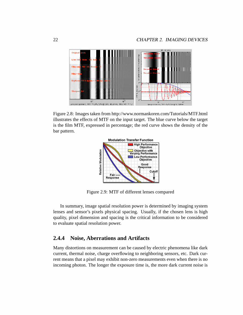
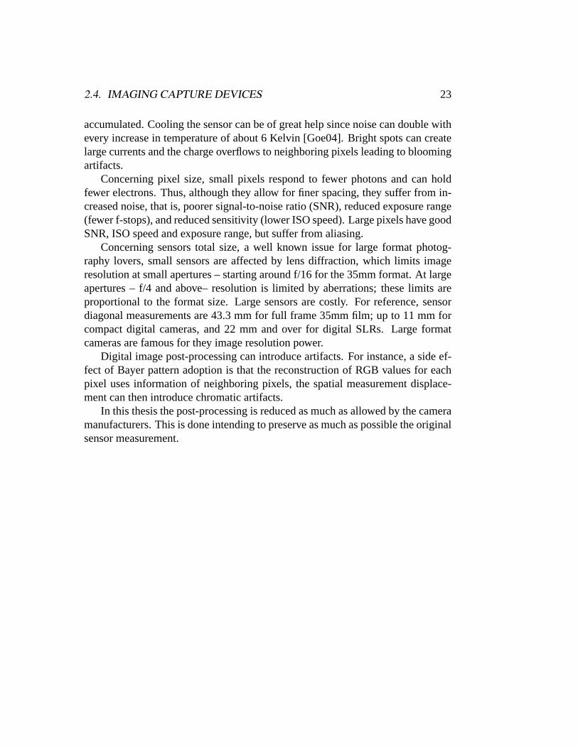
Between light and sensor there is the camera lens system, which has its own reso-lution that influences on the final camera resolution. Lenses, including eye, are notperfect optical systems. As a result when light passes through it undergo a certaindegree of degradation. The Modulation Transfer Function (MTF) (see Figures 2.8and 2.4) shows how well a spatial frequency information is transfered from ob-ject to image. It is the Fourier transform of the point spread function (PSF) thatgives the scattering response to an infinitesimal line of light and is instrumental indetermining the resolution power of a film emulsion or a lens system.
Lens and film manufacturers provide the MTF curves of their lenses and filmemulsions. It is useful for a photographer to interpret these curves, see Figure 2.9,in order to chose which is better for his requirements.
22 CHAPTER 2. IMAGING DEVICES
Figure 2.8: Images taken from http://www.normankoren.com/Tutorials/MTF.htmlillustrates the effects of MTF on the input target. The blue curve below the targetis the film MTF, expressed in percentage; the red curve shows the density of thebar pattern.
Figure 2.9: MTF of different lenses compared
In summary, image spatial resolution power is determined by imaging systemlenses and sensor’s pixels physical spacing. Usually, if the chosen lens is highquality, pixel dimension and spacing is the critical information to be consideredto evaluate spatial resolution power.
2.4.4 Noise, Aberrations and Artifacts
Many distortions on measurement can be caused by electric phenomena like darkcurrent, thermal noise, charge overflowing to neighboring sensors, etc. Dark cur-rent means that a pixel may exhibit non-zero measurements even when there is noincoming photon. The longer the exposure time is, the more dark current noise is
2.4. IMAGING CAPTURE DEVICES 23
accumulated. Cooling the sensor can be of great help since noise can double withevery increase in temperature of about 6 Kelvin [Goe04]. Bright spots can createlarge currents and the charge overflows to neighboring pixels leading to bloomingartifacts.
Concerning pixel size, small pixels respond to fewer photons and can holdfewer electrons. Thus, although they allow for finer spacing, they suffer from in-creased noise, that is, poorer signal-to-noise ratio (SNR), reduced exposure range(fewer f-stops), and reduced sensitivity (lower ISO speed). Large pixels have goodSNR, ISO speed and exposure range, but suffer from aliasing.
Concerning sensors total size, a well known issue for large format photog-raphy lovers, small sensors are affected by lens diffraction, which limits imageresolution at small apertures – starting around f/16 for the 35mm format. At largeapertures – f/4 and above– resolution is limited by aberrations; these limits areproportional to the format size. Large sensors are costly. For reference, sensordiagonal measurements are 43.3 mm for full frame 35mm film; up to 11 mm forcompact digital cameras, and 22 mm and over for digital SLRs. Large formatcameras are famous for they image resolution power.
Digital image post-processing can introduce artifacts. For instance, a side ef-fect of Bayer pattern adoption is that the reconstruction of RGB values for eachpixel uses information of neighboring pixels, the spatial measurement displace-ment can then introduce chromatic artifacts.
In this thesis the post-processing is reduced as much as allowed by the cameramanufacturers. This is done intending to preserve as much as possible the originalsensor measurement.

24 CHAPTER 2. IMAGING DEVICES
Chapter 3
Active Setup
An active setup is composed by a controllable light source that influences on sceneillumination and a camera device. The most commonly used active setup is a paircamera/projector. Technical properties of devices are chosen according to therequirements of the scene of interest. In this work the focus is on objects withdimensions comparable with a vase or a person. In most cases the acquisition isdone in a controlled ambient, which means that background and ambient light canbe controlled.
Digital cameras and projectors devices act like non-linear black-boxes thatconvert light signal into digital images and vice-versa. For these devices to be-come measurement instruments their non-linear behavior must be characterized.
The characterization of device behavior is a calibration process. To calibrate adevice is basically to compare its behavior to some global reference values. In thecase of geometric calibration, for example, the calibration is performed to find thedevice spatial coordinates relatively to a world coordinate system. Analogously,color calibration is usually performed using test targets as global reference values,the task is to classify the device behavior according to these global references.
In some cases global references are more than what is needed, and it is enoughto situate the device behavior relatively to some other device. This is the case ofprojector geometric calibration for active stereo applications: what matters is theprojector position relatively to the camera position; its world coordinates are lessimportant.
In this chapter the devices calibration process and the obtained results of cali-bration of an specific setup is discussed.
25
26 CHAPTER 3. ACTIVE SETUP
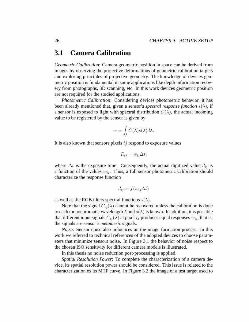
3.1 Camera Calibration
Geometric Calibration: Camera geometric position in space can be derived fromimages by observing the projective deformations of geometric calibration targetsand exploring principles of projective geometry. The knowledge of devices geo-metric position is fundamental in some applications like depth information recov-ery from photographs, 3D scanning, etc. In this work devices geometric positionare not required for the studied applications.
Photometric Calibration: Considering devices photometric behavior, it hasbeen already mentioned that, given a sensor’sspectral response functions(λ), ifa sensor is exposed to light with spectral distributionC(λ), the actual incomingvalue to be registered by the sensor is given by
w =∫
λC(λ)s(λ)dλ.
It is also known that sensors pixelsij respond to exposure values
Eij = wij∆t,
where∆t is the exposure time. Consequently, the actual digitized valuedij isa function of the valueswij. Thus, a full sensor photometric calibration shouldcharacterize the response function
dij = f(wij∆t)
as well as the RGB filters spectral functionss(λ).Note that the signalCij(λ) cannot be recovered unless the calibration is done
to each monochromatic wavelengthλ ands(λ) is known. In addition, it is possiblethat different input signalsCij(λ) at pixelij produces equal responseswij, that is,the signals are sensor’smetamericsignals.
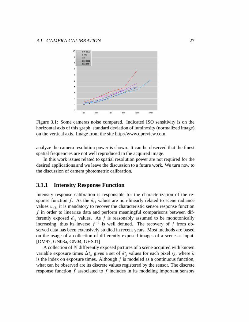
Noise: Sensor noise also influences on the image formation process. In thiswork we referred to technical references of the adopted devices to choose param-eters that minimize sensors noise. In Figure 3.1 the behavior of noise respect tothe chosen ISO sensitivity for different camera models is illustrated.
In this thesis no noise reduction post-processing is applied.Spatial Resolution Power: To complete the characterization of a camera de-
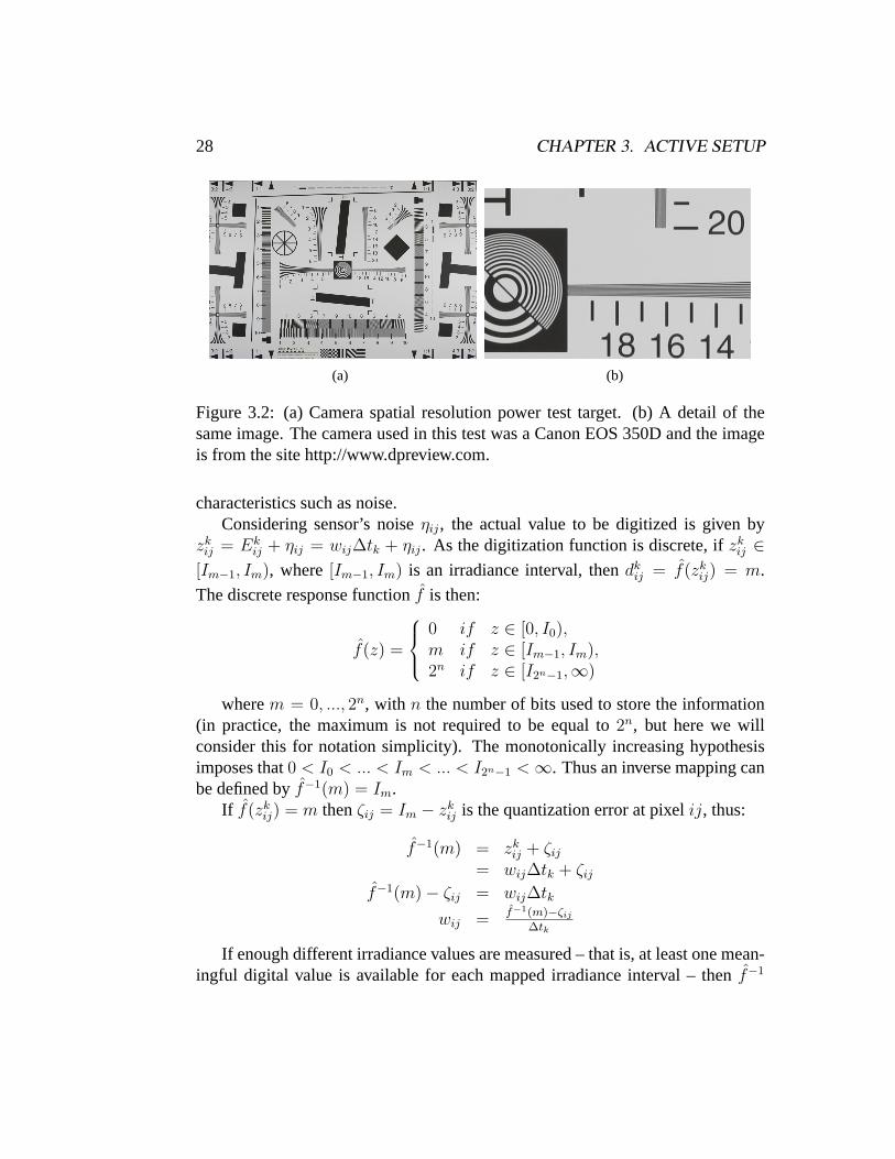
vice, its spatial resolution power should be considered. This issue is related to thecharacterization os its MTF curve. In Figure 3.2 the image of a test target used to
3.1. CAMERA CALIBRATION 27
Figure 3.1: Some cameras noise compared. Indicated ISO sensitivity is on thehorizontal axis of this graph, standard deviation of luminosity (normalized image)on the vertical axis. Image from the site http://www.dpreview.com.
analyze the camera resolution power is shown. It can be observed that the finestspatial frequencies are not well reproduced in the acquired image.
In this work issues related to spatial resolution power are not required for thedesired applications and we leave the discussion to a future work. We turn now tothe discussion of camera photometric calibration.
3.1.1 Intensity Response Function
Intensity response calibration is responsible for the characterization of the re-sponse functionf . As thedij values are non-linearly related to scene radiancevalueswij, it is mandatory to recover the characteristic sensor response functionf in order to linearize data and perform meaningful comparisons between dif-ferently exposeddij values. Asf is reasonably assumed to be monotonicallyincreasing, thus its inversef−1 is well defined. The recovery off from ob-served data has been extensively studied in recent years. Most methods are basedon the usage of a collection of differently exposed images of a scene as input.[DM97, GN03a, GN04, GHS01]
A collection ofN differently exposed pictures of a scene acquired with knownvariable exposure times∆tk gives a set ofdk
ij values for each pixelij, wherekis the index on exposure times. Althoughf is modeled as a continuous function,what can be observed are its discrete values registered by the sensor. The discreteresponse functionf associated tof includes in its modeling important sensors
28 CHAPTER 3. ACTIVE SETUP
(a) (b)
Figure 3.2: (a) Camera spatial resolution power test target. (b) A detail of thesame image. The camera used in this test was a Canon EOS 350D and the imageis from the site http://www.dpreview.com.
characteristics such as noise.Considering sensor’s noiseηij, the actual value to be digitized is given by
zkij = Ek
ij + ηij = wij∆tk + ηij. As the digitization function is discrete, ifzkij ∈
[Im−1, Im), where[Im−1, Im) is an irradiance interval, thendkij = f(zk
ij) = m.
The discrete response functionf is then:
f(z) =
0 if z ∈ [0, I0),m if z ∈ [Im−1, Im),2n if z ∈ [I2n−1,∞)
wherem = 0, ..., 2n, with n the number of bits used to store the information(in practice, the maximum is not required to be equal to2n, but here we willconsider this for notation simplicity). The monotonically increasing hypothesisimposes that0 < I0 < ... < Im < ... < I2n−1 < ∞. Thus an inverse mapping canbe defined byf−1(m) = Im.
If f(zkij) = m thenζij = Im − zk
ij is the quantization error at pixelij, thus:
f−1(m) = zkij + ζij
= wij∆tk + ζij
f−1(m)− ζij = wij∆tk
wij = f−1(m)−ζij
∆tk
If enough different irradiance values are measured – that is, at least one mean-ingful digital value is available for each mapped irradiance interval – thenf−1
3.1. CAMERA CALIBRATION 29
mapping can be recovered for the discretem values. To obtainf in all its continu-ous domain some assumptions must be imposed on the function such as continuityor smoothness restrictions. In some cases parameterized models are used but it canbe too restrictive and some real-world curves may not match the model.
At this point, a question can be posed:What is the essential information nec-essary and sufficient to obtain cameras characteristic response functions fromimages?
In [GN03a] the authors define the intensity mapping functionτ : [0, 1] →[0, 1] as the function that correlates the measured brightness values of two differ-ently exposed images. This function is defined at several discrete points by theaccumulated histogramsH of the images, given byτ(d) = H−1
2 (H1(d)) 1, andexpresses the concept that them brighter pixels in the first image will be thembrighter pixels in the second image for allm 2. Then the following theorem isderived:
Theorem 2 (Intensity Mapping [GN03a]) The histogramh1 of one image, thehistogramh2 of a second image (of the same scene) is necessary and sufficient todetermine the intensity mapping functionτ .
The referred functionτ is given by the relation between two correspondingtones in a pair of images:
Letd1
ij = f(wij∆t1)d2
ij = f(wij∆t2)(3.1)
thend1
ij = f(
f−1(d2ij)
∆t2∆t1
)= f(γf−1(d2
ij))(3.2)
whereγ = ∆t1∆t2
that isd1
ij = f(γf−1(d2ij))
= τ(d2ij)
(3.3)
The answer to the posed question is thatτ , together with the exposure timesratio are necessary and sufficient to recoverf . Here the conclusions were derived
1Supposing that all possible tones are represented in the input image, the respective accumu-lated histogramH is monotonically increasing, thus theH−1 inverse mapping is well defined.
2H and τ are considered as continuous functions although in practice they are observed atdiscrete points and their extension to continuous functions deserves some discussion.
30 CHAPTER 3. ACTIVE SETUP
from an ideal camera sensor without noise. But note thatτ is obtained observ-ing the accumulated histograms, that are less sensitive to noise than the nominalvalues.
Response curvef from observed data
Different approaches can be used to recover thef function from observed data.In what follows some methods will be described. Each of these methods has itsadvantages and drawbacks.
In [DM97], the continuousf is recovered direct from the observed data byfinding a smoothg(dk
ij) = lnf−1(dkij) = lnwij + ln∆tk using an optimization
process. Only a subset of correspondent image pixels from a set of differently ex-posed images are used. The selection of a subset of pixels is needed otherwise theformulated optimization problem would be too large with a lot of redundant in-formation. Then,f−1 is applied to recover the actual scene irradiance by applying
wij =f−1(dk
ij)
∆tk.
In [GN03a], the images accumulated histograms are used to obtain the inten-sity mapping functionτ . Then, a continuousf−1 is obtained assuming that it isa sixth order polynomial, and solving the system given by equationf−1(τ(d)) =γf−1(d) on the coefficients of the polynomial. Two additional restrictions areimposed: that no response is observed if there is no light, that is,f−1(0) = 0,assuming also thatf : [0, 1] → [0, 1], f−1(1) = 1 is fixed, which means that themaximum light intensity leads to the maximum response. Note that there is noguarantee that the obtainedf is monotonically increasing.
The usage of accumulated histograms has some advantages: all the informa-tion present in the image is used instead of a subset of pixels, the images need notto be perfectly registered since spatial information is not present on histograms,and they are less sentive to noise. Note that, if an histogram approach is used,the spatial registration between image pixels is not necessary to findf , but pixelcorrespondences cannot be neglected when reconstructing the Radiance Map.
The same authors, in [GN04], study the space of camera response curves. It isobserved that, although the spaceWRF := f |f(0) = 0, f(1) = 1 andf is mono-tonically increasing of normalized response functions is of infinite-dimension,only a reduced subset of them arise in practice. Based on this observation it iscreated a low-parameter empirical model to the curves, derived from a databaseof real-world camera and film response curves.
In [RBS99] the discrete version of the problem is solved by an iterative op-timization process, an advantage is thatf do not need to be assumed to have a
3.1. CAMERA CALIBRATION 31
shape described by some previously defined class of continuous functions. Theirradiance valueswij and the functionf are optimized at alternated iterations. Asa first step, the quantization errorζk
ij = Im − zkij = Im − wij∆tk is minimized
with respect to the unknownw using
O(I, w) =∑
(i,j),k
σ(m)(Im − wij∆tk)2 (3.4)
The functionσ(m) is a weighting function chosen based on the confidence onthe observed data. In the original paperσ(m) = exp (−4 (m−2n−1)2
(2n−1)2).
By setting the gradient∇O(w) to zero, the optimumw∗ij at pixelij is given by
w∗ij =
∑k σ(m)∆tkIm∑
k σ(m)∆t2k(3.5)
In the initial stepf is supposed to be linear, and theIm values are calculatedusingf . The second step iteratef given thewij. Again the objective function 3.4is minimized, now with respect to the unknownI. The solution is given by:
I∗m =
∑((i,j),k)∈Ωm
wij∆tk
#(Ωm)(3.6)
whereΩm = ((i, j), k) : dkij = m is the index set and#(Ωm) is its cardinal-
ity. A complete iteration of the method is given by calculating 3.5 and 3.6, thenscaling of the result. The process is repeated until some convergence criterion isreached.
We observe that, as originally formulated, there is no guarantee that the valuesIm obtained in 3.6 are monotonically increasing. Especially in the presence ofnoise this assumption can be violated. IfI∗m are not increasing, then the neww∗
ij
can be corrupted, and the method does not converge to the desired radiance map.The correct formulation of the objective function should include the increasingrestrictions:
O(I, w) =∑
(i,j),kσ(m)(Im − wij∆tk)
2
s.a 0 < I0 < · · · < Im < · · · < I2n−1 < ∞(3.7)
This new objective function is not easily solved to the unknownI as the origi-nal one. In the next section the iterative optimization method is applied to recoverthe f response function of the cameras used in the proposed experiments. Theapproaches used to deal with the increasing restrictions will then be discussed.
32 CHAPTER 3. ACTIVE SETUP
Another observation is that although theIm values were modeled as the ex-treme of radiance intervals, the calculatedI∗m are an average of their correspondentradiance values.
3.1.2 Spectral Calibration
The RGB values recorded for a color patch depends not only on light source spec-tral distribution and scenes reflective properties but also on spectral response ofthe filters attached to camera sensors. To interpret meaningfully the RGB valueseach spectral distribution should be characterized separately.
An absolute spectral response calibration is the complete characterization ofRGB filters spectral behavior, that is, to recovers(λ). It would be possible to char-acterizes(λ) if measurements at each monochromatic wavelengthλ were doneseparately, but that is not possible with commonly available light sources.
To the graphical arts and printing industry, color values have to be comparablein order to achieve consistent colors throughout the processing flow. What is donein practice is to adopt a color management systems (CMS) to ensure that colorsremain the same regardless of the device or medium used. The role of a CMS is toprovide a profile for the specific device of interest that allows to convert betweenits color space and standard color spaces. Usually standard color charts are usedto characterize the device color space, in this case, a photograph of the givenchart is taken and based on the registered RGB values the device color space isinferred. The core information of a device profile is in most cases a large lookuptable which allows to encode a wide range of transformations, usually non-linear,between different color spaces [Goe04].
Another issue related to color calibration is the compensation of light sourcespectral distribution. If scene illumination is different from white, what occurswith the most common illuminants like incandescent and fluorescent lighting, thenthe measured values will be biased by the illuminant spectral distribution.
The human eye has a chromatic adaptation mechanism that preserves approx-imately the colors of the scene despite the differences caused by illuminants. Dig-ital imaging systems can not account for these shifts in color balance, and themeasured values should be transformed to compensate for illuminant chromaticdistortions.
Many different algorithms can perform color balancing. A common approachusually referred aswhite balanceis a normalize-to-white approach. There are sev-eral versions of white balance algorithm, but the basic concept is to set at white(WR, WG, WB) a point or a region that should be white in the real scene. One ver-
3.2. PROJECTOR CALIBRATION 33
sion of the white balance algorithm sets values(max(R), max(G), max(B)), themaximum values of the chosen white region, at a reference white(WR, WG, WB).The colors in the image are then transformed using:
(R′, G′, B′) = (WR
max(R)R,
WG
max(G)G,
WB
max(B)B)
In the case of this thesis, the interest is on a relative correlation between aprojector color space and a camera color space, thus no color charts are used.The calibration is done based on projected color information. Regarding whitebalance, we chose to minimize the post-processing of acquired data, thus whitebalancing is not performed. We also assume that in calibration phase, ambientlight is not present. In the case of applications where this assumption is not valid,the adoption of white balance may be reconsidered.
3.2 Projector Calibration
All measurements of projected colors are to be done through the camera. Thusprojector calibration becomes an indirect problem dependent on camera calibra-tion. The camera calibration errors are then propagated to projector calibration.
Geometric Calibration: Light source geometric position can be recovered rel-ative to camera position. If the light source is not included in the camera scenecomposition, the use of mirrors or reflective spheres to localize its position in theambient is useful [Len03]. Projector geometric calibration can benefit from pro-jective principles. A calibration pattern can be projected allowing the recovery ofprojector position by observing projective deformations on the pattern []. In thiswork we are not concerned with geometric calibration.
Photometric Calibration: The actual value emitted by the light source relativeto the projected nominal valueρ is given by its characteristic emitting functionh(ρ), that is reasonably assumed to be monotonically increasing. It is also knownthat to project light in RGB basis, the projector has color filters with characteris-tic spectral emitting functionP (λ). Thus, a full projector photometric calibrationshould characterize the emitting functionh(ρ) as well as the RGB filters spec-tral emitting functionP (λ). The characterization ofP (λ) for each wavelengthrequires specific measurement instruments and cannot be done by using commonphotographic cameras.
Spatial Resolution Power and Noise: To complete the projector behavior char-acterization, issues related to spatial resolution power and noise should also be
34 CHAPTER 3. ACTIVE SETUP
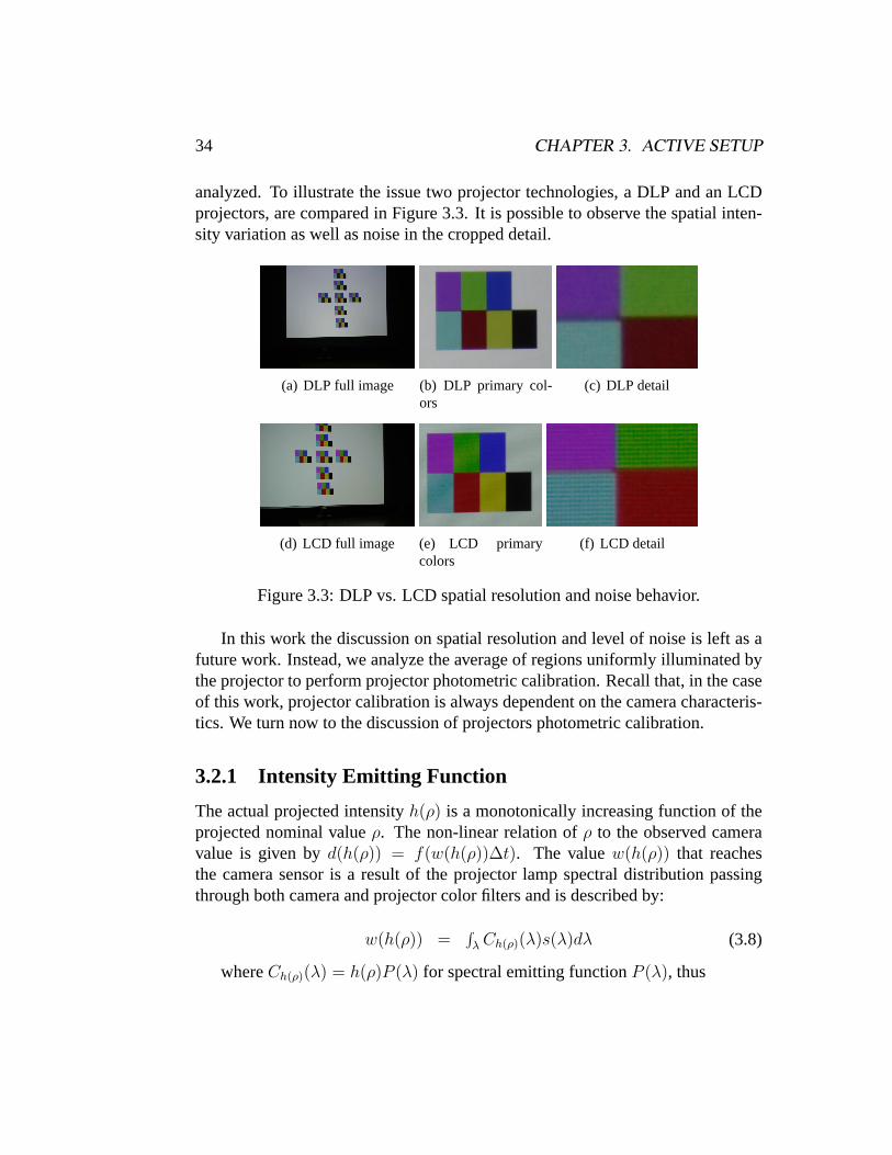
analyzed. To illustrate the issue two projector technologies, a DLP and an LCDprojectors, are compared in Figure 3.3. It is possible to observe the spatial inten-sity variation as well as noise in the cropped detail.
(a) DLP full image (b) DLP primary col-ors
(c) DLP detail
(d) LCD full image (e) LCD primarycolors
(f) LCD detail
Figure 3.3: DLP vs. LCD spatial resolution and noise behavior.
In this work the discussion on spatial resolution and level of noise is left as afuture work. Instead, we analyze the average of regions uniformly illuminated bythe projector to perform projector photometric calibration. Recall that, in the caseof this work, projector calibration is always dependent on the camera characteris-tics. We turn now to the discussion of projectors photometric calibration.
3.2.1 Intensity Emitting Function
The actual projected intensityh(ρ) is a monotonically increasing function of theprojected nominal valueρ. The non-linear relation ofρ to the observed cameravalue is given byd(h(ρ)) = f(w(h(ρ))∆t). The valuew(h(ρ)) that reachesthe camera sensor is a result of the projector lamp spectral distribution passingthrough both camera and projector color filters and is described by:
w(h(ρ)) =∫λ Ch(ρ)(λ)s(λ)dλ (3.8)
whereCh(ρ)(λ) = h(ρ)P (λ) for spectral emitting functionP (λ), thus
3.2. PROJECTOR CALIBRATION 35
w(h(ρ)) =∫λ h(ρ)P (λ)s(λ)dλ (3.9)
It is reasonable to assume thath(ρ) is not dependent onλ. By observingthe projectors technologies we know that a single light source with fixed spectraldistribution passes through RGB pre-defined color filters, this implies that theintensity modulation proportioned byρ should act like a neutral density filter andalters the whole signal in the same way, consequently:
w(h(ρ)) = h(ρ)∫λ P (λ)s(λ)dλ (3.10)
For an RGB based system the camera has three spectral response curvessq(λ),whereq = R,G orB, as well as projector has three spectral emitting curvesPr(λ)wherer = R,G or B. This gives rise to nineSq
r (λ) combined spectral curves thatcharacterize the pair camera/projector, in addition, as the spectral functions arefixed, nine constant factors arise:
κqr =
∫λPq(λ)sr(λ)dλ =
∫λSq
r (λ)dλ
For an ideal camera/projector pairκqr = 0 if q 6= r. Assuming that ambient
light is set to zero, the projector become the only scene illuminant. It is reasonableto assume thath is the same for all the three channels by observing the projectorstechnologies described in previous Chapter. For each emitted intensityh(ρ), thereis a correspondentw(h(ρ)) value, both have three channels of information, thatis, the system that relates the actual projected intensity to the intensity values thatreaches the sensor is linear and given by: wR
wG
wB
︸ ︷︷ ︸
w
=
κRR κR
G κRB
κGR κG
G κGB
κBR κB
G κBB
︸ ︷︷ ︸
K
h(ρR)h(ρG)h(ρB)
︸ ︷︷ ︸
h(ρ)
The matrixK characterizes the spectral behavior of the pair camera/projector,and it will be referred as thespectral characteristic matrix. It is expected thatK is near diagonal, that is,κq
r ≈ 0 if q 6= r, and all its entries are nonnega-tive, in addition, its diagonal entries should be strictly positive. For ideal pairscamera/projectorK is the identity.
Ambient light can be added to the model by summing up its contribution:
w = Kh(ρ) + c (3.11)

36 CHAPTER 3. ACTIVE SETUP
Emitting curve f from observed data
It is easy to see that ifK is known, then thecharacteristic emitting functionh(ρ)is recovered from observations by solving the systemw(h(ρ)) = Kh(ρ). Theproblem is thatK is also unknown, and the complete calibration process shouldrecover the emitting functionh(ρ) as well as the spectral characteristic matrixK.In addition,h is not necessarily linear, thus the problem on the unknownsK andh is non-linear.
The solution can be iteratively approximated by minimizing error solving anon-linear least squares problems given byerr = Kh(ρ)−w. An initial solutionto the problem can be produced solving its linear version, that is,w = Kρ.
3.3 Calibration in Practice
The calibration of an active setup involve the camera calibration and the lightsource calibration, in our case, a projector. In applications different set-ups wereused, in what follows our photographic setup will be described and calibrated.This set-up uses a photographic camera and two types of digital projectors.Setupa: Camera plus LCD projector (illustred in Figure 3.4).Setup b: Camera plusDLP projector.
Figure 3.4: Our photographic setup.
A diffuse white screen was used to project images during the calibration pro-cess.
3.3.1 Camera Calibration
The digital camera used in our calibration tests is a Canon EOS D350. In theexperiments we vary image exposure by controlling acquisition time or by con-
3.3. CALIBRATION IN PRACTICE 37
trolling illumination, while all other parameters were kept fixed. The camera pa-rameters were set to:
• lens aperture = 22F,
• ISO speed = 200,
• focal distance = 41 mm,
• image size =3456× 2304 pixels - RAW.
All other parameters were turned off to minimize image processing.Images were captured in RAW 12 bits proprietary camera format and con-
verted to TIF 16 bits image by theDigital Photo Professional 1.6software at-tempting to turn off all unnecessary additional processing.
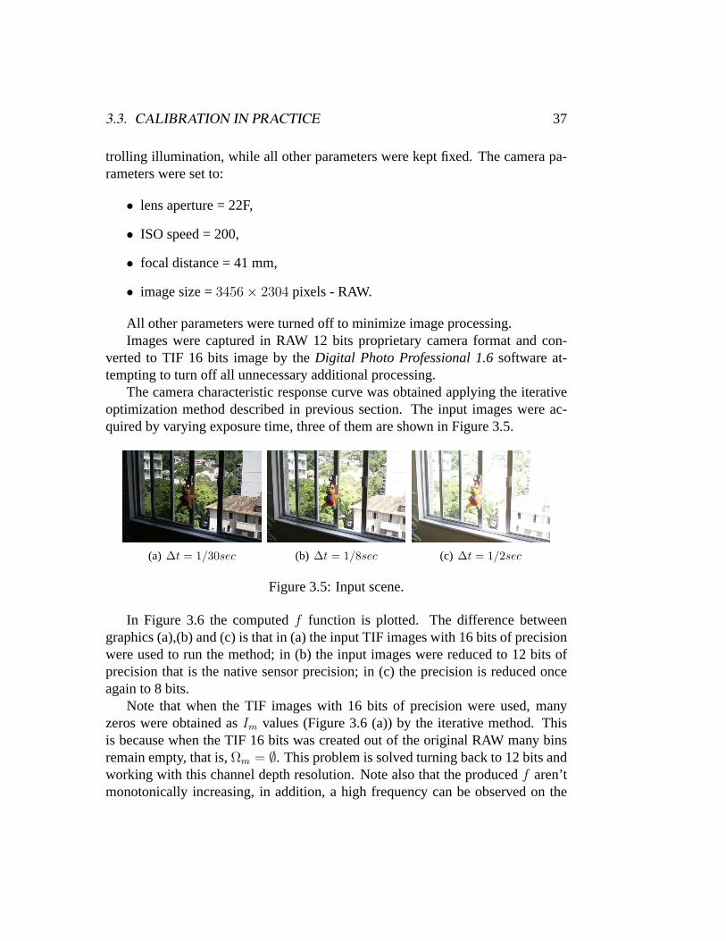
The camera characteristic response curve was obtained applying the iterativeoptimization method described in previous section. The input images were ac-quired by varying exposure time, three of them are shown in Figure 3.5.
(a) ∆t = 1/30sec (b) ∆t = 1/8sec (c) ∆t = 1/2sec
Figure 3.5: Input scene.
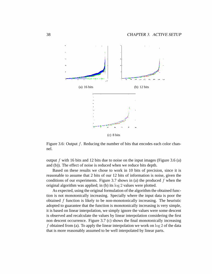
In Figure 3.6 the computedf function is plotted. The difference betweengraphics (a),(b) and (c) is that in (a) the input TIF images with 16 bits of precisionwere used to run the method; in (b) the input images were reduced to 12 bits ofprecision that is the native sensor precision; in (c) the precision is reduced onceagain to 8 bits.
Note that when the TIF images with 16 bits of precision were used, manyzeros were obtained asIm values (Figure 3.6 (a)) by the iterative method. Thisis because when the TIF 16 bits was created out of the original RAW many binsremain empty, that is,Ωm = ∅. This problem is solved turning back to 12 bits andworking with this channel depth resolution. Note also that the producedf aren’tmonotonically increasing, in addition, a high frequency can be observed on the
38 CHAPTER 3. ACTIVE SETUP
(a) 16 bits (b) 12 bits
(c) 8 bits
Figure 3.6: Outputf . Reducing the number of bits that encodes each color chan-nel.
outputf with 16 bits and 12 bits due to noise on the input images (Figure 3.6 (a)and (b)). The effect of noise is reduced when we reduce bits depth.
Based on these results we chose to work in 10 bits of precision, since it isreasonable to assume that 2 bits of our 12 bits of information is noise, given theconditions of our experiments. Figure 3.7 shows in (a) the producedf when theoriginal algorithm was applied; in (b) itslog 2 values were plotted.
As expected, using the original formulation of the algorithm the obtained func-tion is not monotonically increasing. Specially where the input data is poor theobtainedf function is likely to be non-monotonically increasing. The heuristicadopted to guarantee that the function is monotonically increasing is very simple,it is based on linear interpolation, we simply ignore the values were some descentis observed and recalculate the values by linear interpolation considering the firstnon descent occurrence. Figure 3.7 (c) shows the final monotonically increasingf obtained from (a). To apply the linear interpolation we work onlog 2 of the datathat is more reasonably assumed to be well interpolated by linear parts.

3.3. CALIBRATION IN PRACTICE 39
(a) 10 bits (b) 10 bits - log2
(c) monotonically increasingf
Figure 3.7: Outputf 10 bits of pixel depth.
3.3.2 Projector Calibration
Not only different cameras register different brightness values for the same inputexposure, projectors emission characteristics also depends on projector technol-ogy, model and time of use. The projectors used in our experiments were a LCDMitsubishi SL4SU and a DLP InFocus LP70. We now analyze our projectors bycalibrating them respect to the previously calibrated camera.
The camera parameters were fixed after photometering the white screen witha constant gray pattern being projected. The screen plane was initially focusedusing the camera auto-focus facility and then the auto-focus was turned off andkept fixed during the experiment. The camera characteristic functionf−1 wasapplied to the nominal camera values to obtain the linearizedw values.
To recover the characteristic emitting functionh(ρ) at some specific valuesρ,and the spectral characteristic matrixK, Projected intensity was modulated forthe primary colors and the values registered by the camera observed. In Figure3.8 the projected green values for the DLP projector are shown.
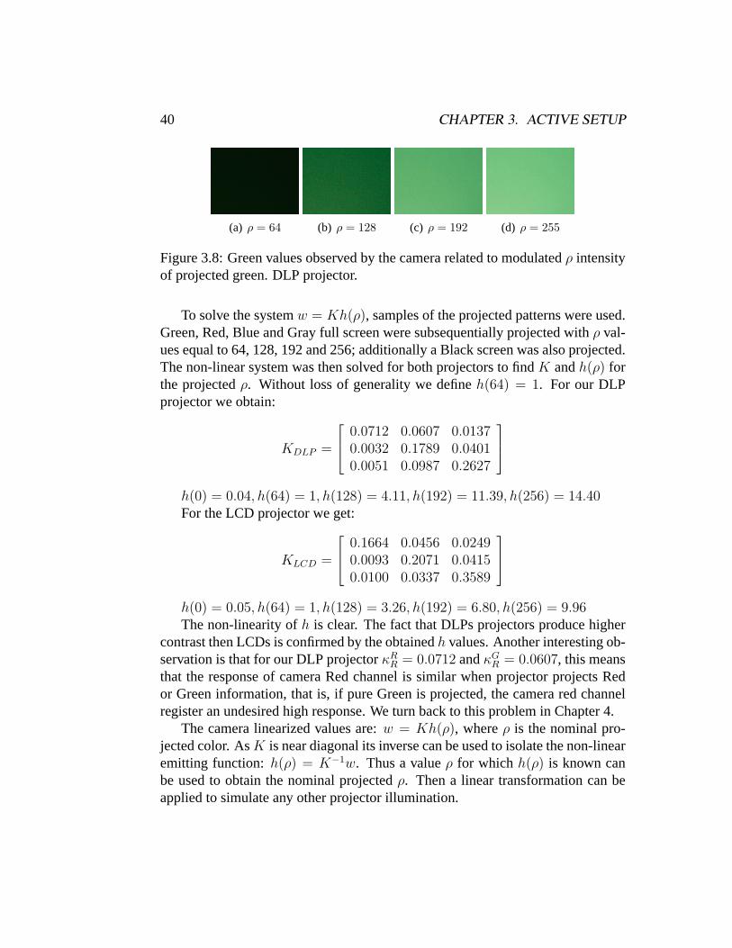
40 CHAPTER 3. ACTIVE SETUP
(a) ρ = 64 (b) ρ = 128 (c) ρ = 192 (d) ρ = 255
Figure 3.8: Green values observed by the camera related to modulatedρ intensityof projected green. DLP projector.
To solve the systemw = Kh(ρ), samples of the projected patterns were used.Green, Red, Blue and Gray full screen were subsequentially projected withρ val-ues equal to 64, 128, 192 and 256; additionally a Black screen was also projected.The non-linear system was then solved for both projectors to findK andh(ρ) forthe projectedρ. Without loss of generality we defineh(64) = 1. For our DLPprojector we obtain:
KDLP =
0.0712 0.0607 0.01370.0032 0.1789 0.04010.0051 0.0987 0.2627
h(0) = 0.04, h(64) = 1, h(128) = 4.11, h(192) = 11.39, h(256) = 14.40For the LCD projector we get:
KLCD =
0.1664 0.0456 0.02490.0093 0.2071 0.04150.0100 0.0337 0.3589
h(0) = 0.05, h(64) = 1, h(128) = 3.26, h(192) = 6.80, h(256) = 9.96The non-linearity ofh is clear. The fact that DLPs projectors produce higher
contrast then LCDs is confirmed by the obtainedh values. Another interesting ob-servation is that for our DLP projectorκR
R = 0.0712 andκGR = 0.0607, this means
that the response of camera Red channel is similar when projector projects Redor Green information, that is, if pure Green is projected, the camera red channelregister an undesired high response. We turn back to this problem in Chapter 4.
The camera linearized values are:w = Kh(ρ), whereρ is the nominal pro-jected color. AsK is near diagonal its inverse can be used to isolate the non-linearemitting function:h(ρ) = K−1w. Thus a valueρ for which h(ρ) is known canbe used to obtain the nominal projectedρ. Then a linear transformation can beapplied to simulate any other projector illumination.
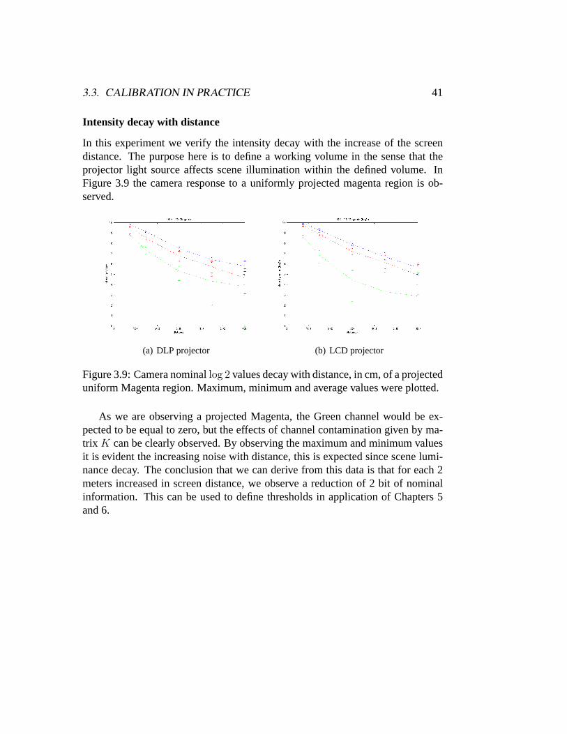
3.3. CALIBRATION IN PRACTICE 41
Intensity decay with distance
In this experiment we verify the intensity decay with the increase of the screendistance. The purpose here is to define a working volume in the sense that theprojector light source affects scene illumination within the defined volume. InFigure 3.9 the camera response to a uniformly projected magenta region is ob-served.
(a) DLP projector (b) LCD projector
Figure 3.9: Camera nominallog 2 values decay with distance, in cm, of a projecteduniform Magenta region. Maximum, minimum and average values were plotted.
As we are observing a projected Magenta, the Green channel would be ex-pected to be equal to zero, but the effects of channel contamination given by ma-trix K can be clearly observed. By observing the maximum and minimum valuesit is evident the increasing noise with distance, this is expected since scene lumi-nance decay. The conclusion that we can derive from this data is that for each 2meters increased in screen distance, we observe a reduction of 2 bit of nominalinformation. This can be used to define thresholds in application of Chapters 5and 6.

42 CHAPTER 3. ACTIVE SETUP
Chapter 4
Stereo Correspondence
Shape acquisition is one of the fundamental tasks in 3D photography. An objectcan be thought of as made up of a collection of surfaces which in turn have geo-metric properties such as curvature and features as well as photometric propertiessuch as color, texture and material reflectance. In the last two decades the prob-lem of accurately capturing an object’s geometry was extensively studied, whilethe acquisition of high-quality textures, an equally important problem, only inrecent years has become subject of research.
The recovery of an object’s 3D shape is an inverse problem usually subdividedin several subproblems:depth acquisition, alignment of views, mesh reconstruc-tion, etc.
The depth acquisitionis the recovery of a depth map given an image or aset of images of a scene; it is heavily dependent on the hardware set-up chosento acquire the images. Thealignment of viewsis the problem of given a set ofdepth maps acquired from distinct points of view, construct a cloud of points thatconsistently represents the object; it is dependent on the knowledge of camerapositions and on initial solutions. Texture information can help in this step. Themesh reconstructionis responsible for given a cloud of points construct a meshthat describes the object. This step can be substituted by the direct visualizationof a cloud of points.
This chapter focus ondepth acquisitiontechniques. The reasoning that al-low depth recovery is based on the observation of how depth influences on theimage formation. Observing how a controlled light source produces shadows weget shape from shading algorithms, observing the behavior of image focus we getdepth from focus, observing images from different points of view we get stereotechniques. A classification of shape acquisition methods is given in Figure 4.1.
43
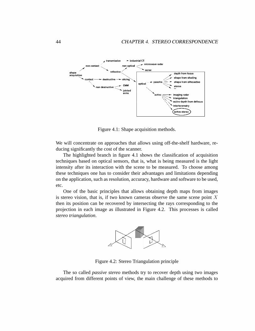
44 CHAPTER 4. STEREO CORRESPONDENCE
Figure 4.1: Shape acquisition methods.
We will concentrate on approaches that allows using off-the-shelf hardware, re-ducing significantly the cost of the scanner.
The highlighted branch in figure 4.1 shows the classification of acquisitiontechniques based on optical sensors, that is, what is being measured is the lightintensity after its interaction with the scene to be measured. To choose amongthese techniques one has to consider their advantages and limitations dependingon the application, such as resolution, accuracy, hardware and software to be used,etc.
One of the basic principles that allows obtaining depth maps from imagesis stereo vision, that is, if two known cameras observe the same scene pointXthen its position can be recovered by intersecting the rays corresponding to theprojection in each image as illustrated in Figure 4.2. This processes is calledstereo triangulation.
Figure 4.2: Stereo Triangulation principle
The so calledpassive stereomethods try to recover depth using two imagesacquired from different points of view, the main challenge of these methods to
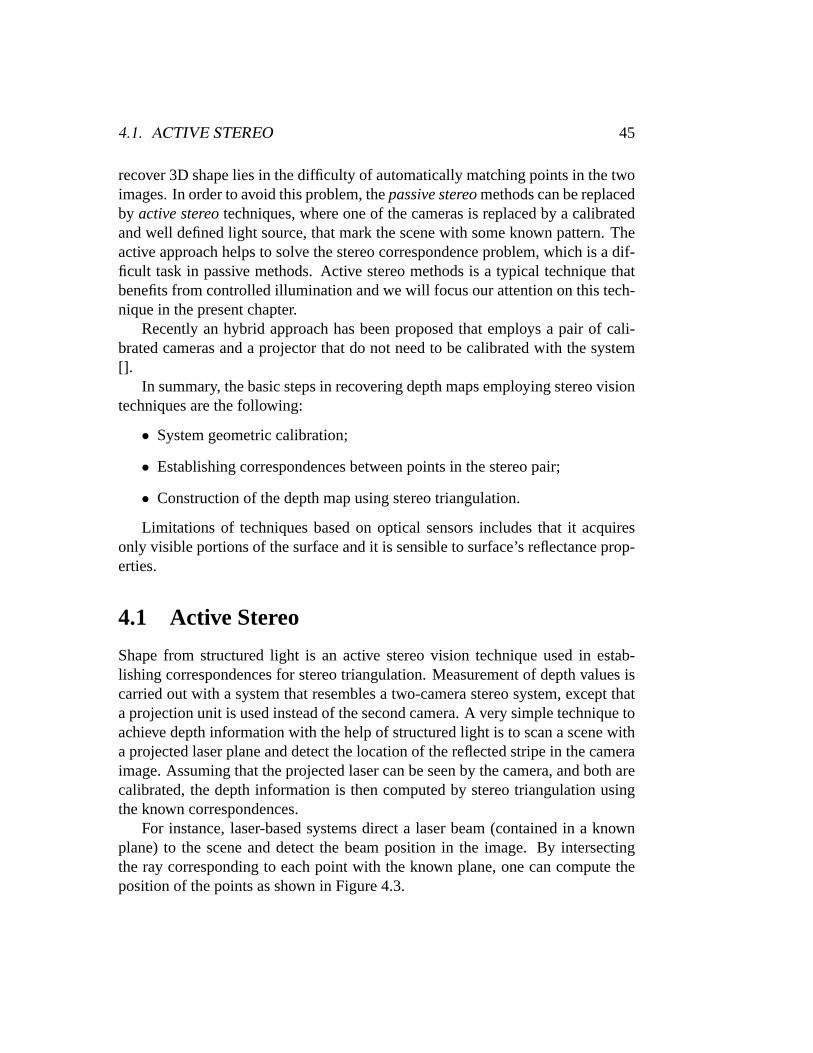
4.1. ACTIVE STEREO 45
recover 3D shape lies in the difficulty of automatically matching points in the twoimages. In order to avoid this problem, thepassive stereomethods can be replacedby active stereotechniques, where one of the cameras is replaced by a calibratedand well defined light source, that mark the scene with some known pattern. Theactive approach helps to solve the stereo correspondence problem, which is a dif-ficult task in passive methods. Active stereo methods is a typical technique thatbenefits from controlled illumination and we will focus our attention on this tech-nique in the present chapter.
Recently an hybrid approach has been proposed that employs a pair of cali-brated cameras and a projector that do not need to be calibrated with the system[].
In summary, the basic steps in recovering depth maps employing stereo visiontechniques are the following:
• System geometric calibration;
• Establishing correspondences between points in the stereo pair;
• Construction of the depth map using stereo triangulation.
Limitations of techniques based on optical sensors includes that it acquiresonly visible portions of the surface and it is sensible to surface’s reflectance prop-erties.
4.1 Active Stereo
Shape from structured light is an active stereo vision technique used in estab-lishing correspondences for stereo triangulation. Measurement of depth values iscarried out with a system that resembles a two-camera stereo system, except thata projection unit is used instead of the second camera. A very simple technique toachieve depth information with the help of structured light is to scan a scene witha projected laser plane and detect the location of the reflected stripe in the cameraimage. Assuming that the projected laser can be seen by the camera, and both arecalibrated, the depth information is then computed by stereo triangulation usingthe known correspondences.
For instance, laser-based systems direct a laser beam (contained in a knownplane) to the scene and detect the beam position in the image. By intersectingthe ray corresponding to each point with the known plane, one can compute theposition of the points as shown in Figure 4.3.
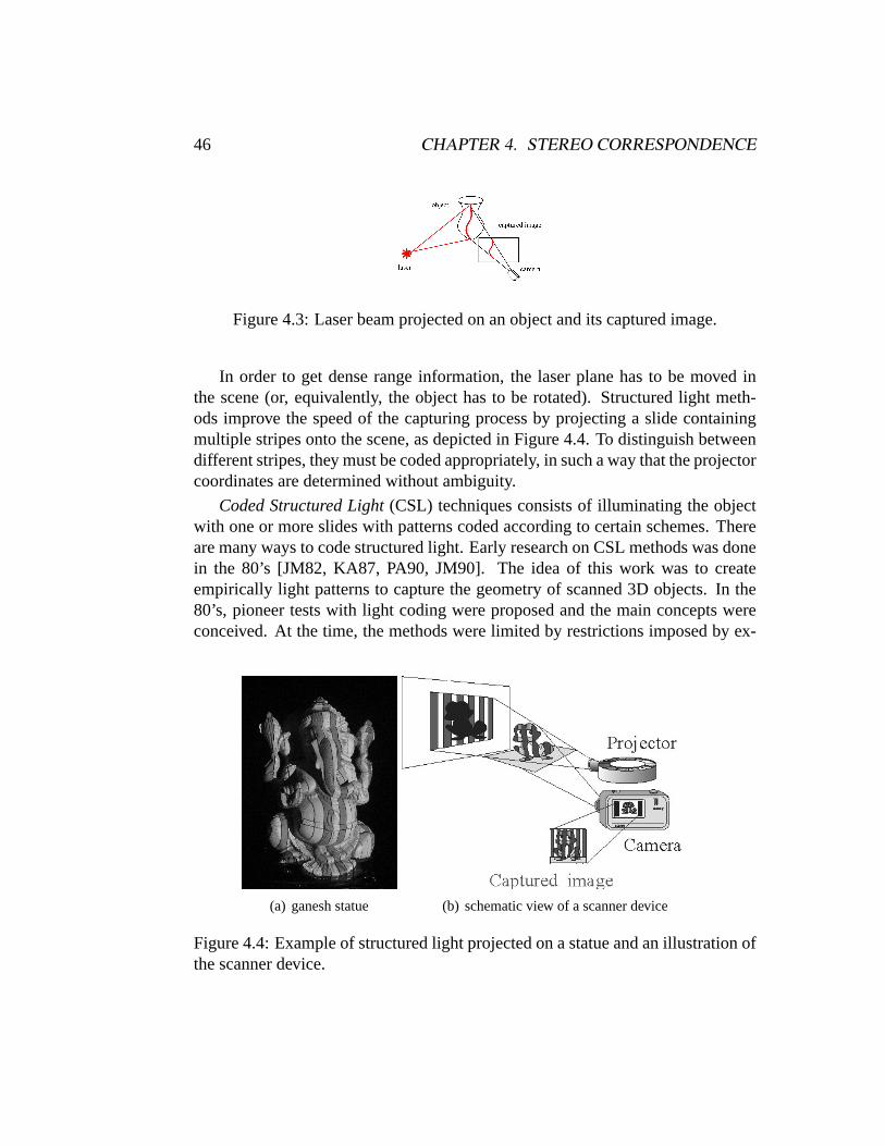
46 CHAPTER 4. STEREO CORRESPONDENCE
Figure 4.3: Laser beam projected on an object and its captured image.
In order to get dense range information, the laser plane has to be moved inthe scene (or, equivalently, the object has to be rotated). Structured light meth-ods improve the speed of the capturing process by projecting a slide containingmultiple stripes onto the scene, as depicted in Figure 4.4. To distinguish betweendifferent stripes, they must be coded appropriately, in such a way that the projectorcoordinates are determined without ambiguity.
Coded Structured Light(CSL) techniques consists of illuminating the objectwith one or more slides with patterns coded according to certain schemes. Thereare many ways to code structured light. Early research on CSL methods was donein the 80’s [JM82, KA87, PA90, JM90]. The idea of this work was to createempirically light patterns to capture the geometry of scanned 3D objects. In the80’s, pioneer tests with light coding were proposed and the main concepts wereconceived. At the time, the methods were limited by restrictions imposed by ex-
(a) ganesh statue (b) schematic view of a scanner device
Figure 4.4: Example of structured light projected on a statue and an illustration ofthe scanner device.
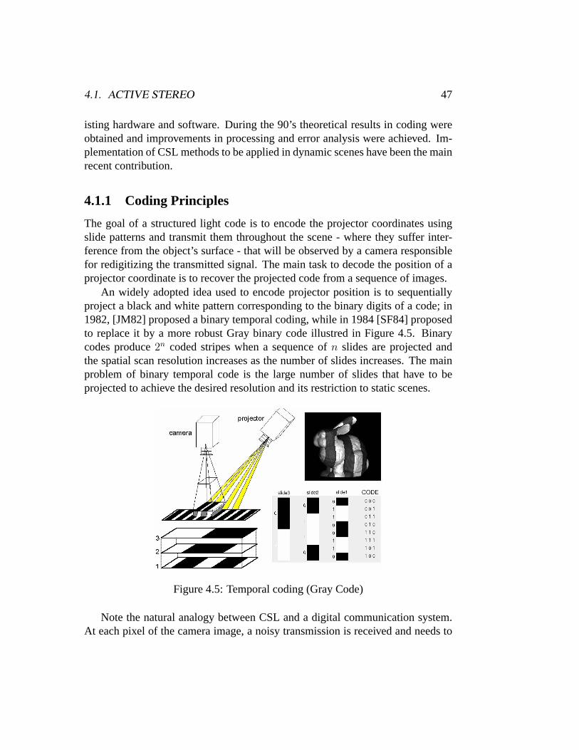
4.1. ACTIVE STEREO 47
isting hardware and software. During the 90’s theoretical results in coding wereobtained and improvements in processing and error analysis were achieved. Im-plementation of CSL methods to be applied in dynamic scenes have been the mainrecent contribution.
4.1.1 Coding Principles
The goal of a structured light code is to encode the projector coordinates usingslide patterns and transmit them throughout the scene - where they suffer inter-ference from the object’s surface - that will be observed by a camera responsiblefor redigitizing the transmitted signal. The main task to decode the position of aprojector coordinate is to recover the projected code from a sequence of images.
An widely adopted idea used to encode projector position is to sequentiallyproject a black and white pattern corresponding to the binary digits of a code; in1982, [JM82] proposed a binary temporal coding, while in 1984 [SF84] proposedto replace it by a more robust Gray binary code illustred in Figure 4.5. Binarycodes produce2n coded stripes when a sequence ofn slides are projected andthe spatial scan resolution increases as the number of slides increases. The mainproblem of binary temporal code is the large number of slides that have to beprojected to achieve the desired resolution and its restriction to static scenes.
Figure 4.5: Temporal coding (Gray Code)
Note the natural analogy between CSL and a digital communication system.At each pixel of the camera image, a noisy transmission is received and needs to
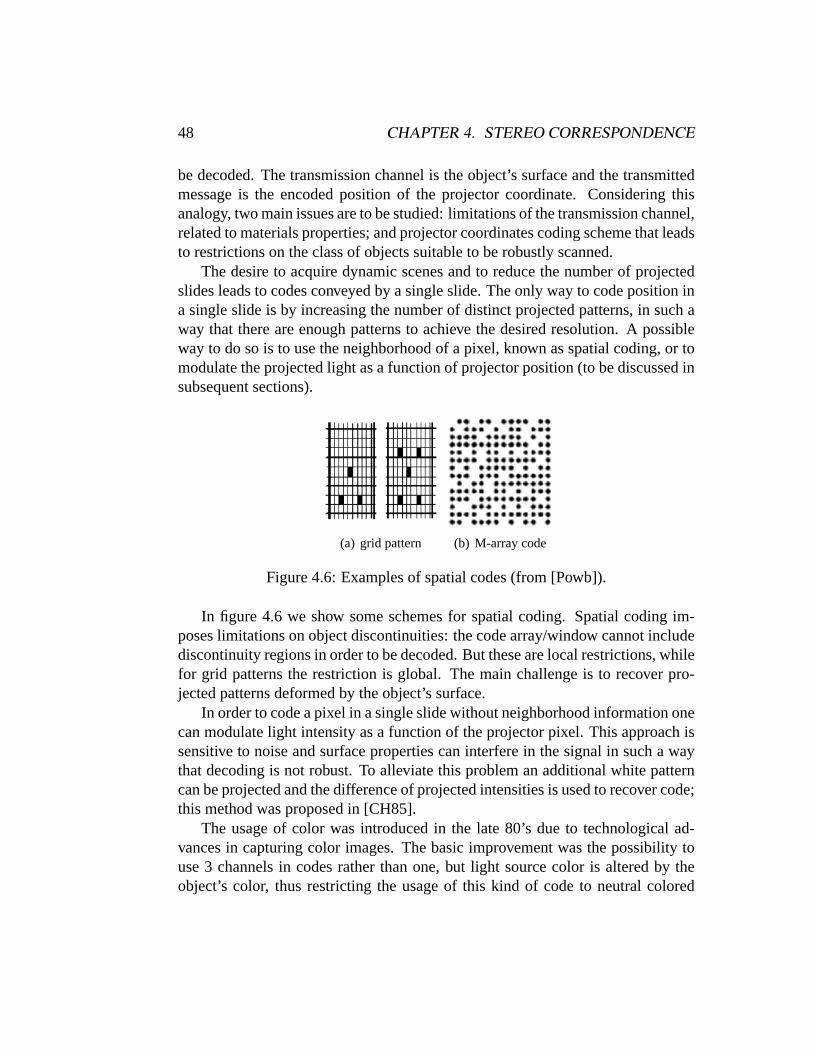
48 CHAPTER 4. STEREO CORRESPONDENCE
be decoded. The transmission channel is the object’s surface and the transmittedmessage is the encoded position of the projector coordinate. Considering thisanalogy, two main issues are to be studied: limitations of the transmission channel,related to materials properties; and projector coordinates coding scheme that leadsto restrictions on the class of objects suitable to be robustly scanned.
The desire to acquire dynamic scenes and to reduce the number of projectedslides leads to codes conveyed by a single slide. The only way to code position ina single slide is by increasing the number of distinct projected patterns, in such away that there are enough patterns to achieve the desired resolution. A possibleway to do so is to use the neighborhood of a pixel, known as spatial coding, or tomodulate the projected light as a function of projector position (to be discussed insubsequent sections).
(a) grid pattern (b) M-array code
Figure 4.6: Examples of spatial codes (from [Powb]).
In figure 4.6 we show some schemes for spatial coding. Spatial coding im-poses limitations on object discontinuities: the code array/window cannot includediscontinuity regions in order to be decoded. But these are local restrictions, whilefor grid patterns the restriction is global. The main challenge is to recover pro-jected patterns deformed by the object’s surface.
In order to code a pixel in a single slide without neighborhood information onecan modulate light intensity as a function of the projector pixel. This approach issensitive to noise and surface properties can interfere in the signal in such a waythat decoding is not robust. To alleviate this problem an additional white patterncan be projected and the difference of projected intensities is used to recover code;this method was proposed in [CH85].
The usage of color was introduced in the late 80’s due to technological ad-vances in capturing color images. The basic improvement was the possibility touse 3 channels in codes rather than one, but light source color is altered by theobject’s color, thus restricting the usage of this kind of code to neutral colored
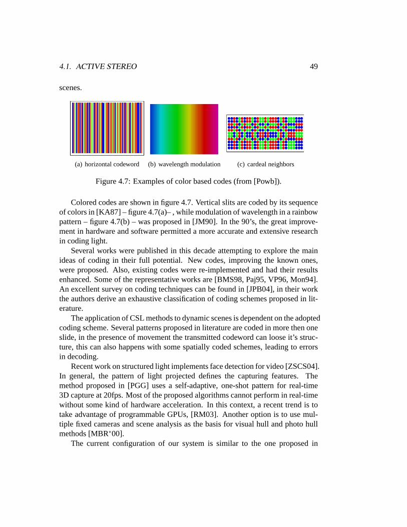
4.1. ACTIVE STEREO 49
scenes.
(a) horizontal codeword (b) wavelength modulation (c) cardeal neighbors
Figure 4.7: Examples of color based codes (from [Powb]).
Colored codes are shown in figure 4.7. Vertical slits are coded by its sequenceof colors in [KA87] – figure 4.7(a)– , while modulation of wavelength in a rainbowpattern – figure 4.7(b) – was proposed in [JM90]. In the 90’s, the great improve-ment in hardware and software permitted a more accurate and extensive researchin coding light.
Several works were published in this decade attempting to explore the mainideas of coding in their full potential. New codes, improving the known ones,were proposed. Also, existing codes were re-implemented and had their resultsenhanced. Some of the representative works are [BMS98, Paj95, VP96, Mon94].An excellent survey on coding techniques can be found in [JPB04], in their workthe authors derive an exhaustive classification of coding schemes proposed in lit-erature.
The application of CSL methods to dynamic scenes is dependent on the adoptedcoding scheme. Several patterns proposed in literature are coded in more then oneslide, in the presence of movement the transmitted codeword can loose it’s struc-ture, this can also happens with some spatially coded schemes, leading to errorsin decoding.
Recent work on structured light implements face detection for video [ZSCS04].In general, the pattern of light projected defines the capturing features. Themethod proposed in [PGG] uses a self-adaptive, one-shot pattern for real-time3D capture at 20fps. Most of the proposed algorithms cannot perform in real-timewithout some kind of hardware acceleration. In this context, a recent trend is totake advantage of programmable GPUs, [RM03]. Another option is to use mul-tiple fixed cameras and scene analysis as the basis for visual hull and photo hullmethods [MBR∗00].
The current configuration of our system is similar to the one proposed in
50 CHAPTER 4. STEREO CORRESPONDENCE
[OHS01], [SM02], however, our implementation for video is more efficient dueto the (6,2(2))-BCSL color code, that allows to robustly obtain a 3D video streamwith texture and depth information at 30fps [VSVC05]. The data processing mod-ule extracts depth information from structured light code. The visualization mod-ule renders 3D video using the geometry induced by the color code used.
Texture recovery is usually done as a separate acquisition step, after acquisi-tion the geometry and texture needs to be registered to each other. Acquiring bothat the same time the registration problem is avoided.
4.1.2 Taxonomy
As we saw in previous sections, the three ways to code projected light are the useof chromatic, spatial or temporal modulation in the illumination intensity pattern.A taxonomy of CSL proposed in [OHS01] considering differences between pat-terns and the restrictions that they impose on the scene to be scanned. Chromaticmodulation imposes restrictions on the allowable colors in the scene. When spa-tial coding is used, local continuity of the scene is necessary for recovering thetransmitted code. Conversely, temporal coding restricts motion of the scene.
To encode information we have to decide how to describe the information interms of the signal to be transmitted. The nature of the signal will define possibleletters of an alphabetwhile the rule for concatenating letters definescodewords.The main tools to design the code are the number of distinct symbols (basic sig-nals) available, the size of the codeword made by these symbols and, in the caseof spatial coding, the structure of the neighborhood used to define a codeword.
In light coding the levels of intensity modulation and the number of channelsconsidered (usually 1 or 3 channels) forms the alphabet letters, while codewordscan be formed by temporal or spatial concatenation of letters. Accurate trans-mission of this alphabet requires that the material properties of objects present onthe scene do not distort intensities or chroma too much, while the correct trans-mission of the codeword structure depends on scene’s properties, that is, spatialconcatenation of codewords can be lost if discontinuities are present on surface onwhich one is projecting the code, while robust decoding of temporal concatenationrestricts scene’s movement.
This reasoning leads to a simplea priori classification of codes, that is, basedon decision made in designing the code since it imposes restrictions on the sceneto be scanned, in contrast to the usuala posterioriclassification of coding, likethe complete classification proposed in [JPB04]. Our classification is based onthe following observations of the proposed code design:

4.1. ACTIVE STEREO 51
• available alphabet symbols→ restricts scene’s reflectivity
– levels of light intensity modulation
– number of channels used
• rules for letters concatenation: codeword structure
– temporal→ restricts scene’s changes in time
– spatial→ restricts scene’s depth discontinuities
Comparing our classification to the one given in [JPB04], we associate theirscene applicabilityas a consequence of the usage of temporal coding, theirpixeldepthis related to the choice of the alphabet for coding (number of channels usedand levels of intensity modulation), and finally thecoding strategyis a conse-quence of the numbers of codeword generated by the codeword schema. Strictlytemporal coding (as Gray code) is then applicable on static scenes but imposes nospatial nor reflectance restrictions on scanned objects; the codeword produced isbinary and produces2s words wheres is the number of projected slides. Spatio-temporal coding, as proposed in [OHS01], attempt to reduce the number of pro-jected slides using weak spatial restrictions.
We classify CSL methods by observing the code design since it is the code de-sign that imposes restrictions on the scene (or transmission channel) to be scanned.That is, if we use spatial coding, the scene has to preserve the spatial structure;otherwise, there will be loss of information. In the scene this can be translatedas local continuity. The main characteristics of code design are the number ofdistinct symbols (basic signals), the size of the word made by symbols and, inthe case of spatial coding, the geometry used. The following table classifies somecodes proposed in literature.
We observe that code spatial structure of coding will be lost if discontinuitiesare present on projected surface area. Also, it is necessary to recover accuratelyintensity modulations, which requires that the surface does not distort intensitiesor chroma too much. Finally, the size of the codeword imposes that movement isnot allowed while the codeword is not completed.
An improvement in spatial coding is proposed in [OHS01], where a CSLscheme is based on stripe boundaries. The codes are associated with pairs ofstripes, instead of with the stripes themselves as in traditional methods. Boundary
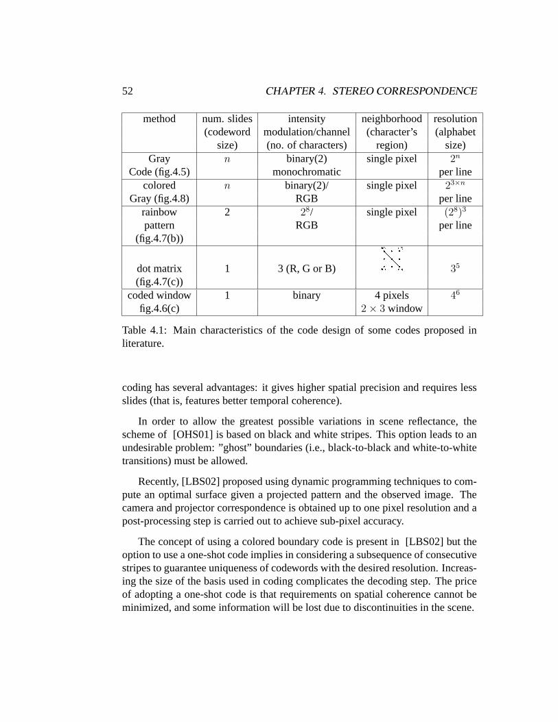
52 CHAPTER 4. STEREO CORRESPONDENCE
method num. slides intensity neighborhood resolution(codeword modulation/channel (character’s (alphabet
size) (no. of characters) region) size)Gray n binary(2) single pixel 2n
Code (fig.4.5) monochromatic per linecolored n binary(2)/ single pixel 23×n
Gray (fig.4.8) RGB per linerainbow 2 28/ single pixel (28)3
pattern RGB per line(fig.4.7(b))
dot matrix 1 3 (R, G or B) 35
(fig.4.7(c))coded window 1 binary 4 pixels 46
fig.4.6(c) 2× 3 window
Table 4.1: Main characteristics of the code design of some codes proposed inliterature.
coding has several advantages: it gives higher spatial precision and requires lessslides (that is, features better temporal coherence).
In order to allow the greatest possible variations in scene reflectance, thescheme of [OHS01] is based on black and white stripes. This option leads to anundesirable problem: ”ghost” boundaries (i.e., black-to-black and white-to-whitetransitions) must be allowed.
Recently, [LBS02] proposed using dynamic programming techniques to com-pute an optimal surface given a projected pattern and the observed image. Thecamera and projector correspondence is obtained up to one pixel resolution and apost-processing step is carried out to achieve sub-pixel accuracy.
The concept of using a colored boundary code is present in [LBS02] but theoption to use a one-shot code implies in considering a subsequence of consecutivestripes to guarantee uniqueness of codewords with the desired resolution. Increas-ing the size of the basis used in coding complicates the decoding step. The priceof adopting a one-shot code is that requirements on spatial coherence cannot beminimized, and some information will be lost due to discontinuities in the scene.
4.2. MINIMAL CODE DESIGN 53
4.2 Minimal Code Design
When designing a CSL we have two conflicting objectives: one is to generateenough distinct codewords to encode projector coordinates without ambiguity,what is achieved augmenting spatial and temporal neighborhood or increasing thenumber of alphabet symbols; the other is to reduce the restrictions imposed onthe scene to be scanned. We are then challenged to find a minimal code in termsof restrictions while getting a maximal possible number of distinct codewords.What is minimal in this sense? The answer is: a temporal neighborhoods = 2,a spatial neighborhood that considers only one neighbor, that is achieved codingboundaries, and finally using a binary light intensity modulation that guarantees arobust recovery of the transmitted information. The coding proposed in [OHS01]is one step in this direction except for the fact that their temporal neighborhoodis s = 4. Our proposal, to be described in the following sections, is the usage ofthe 3 color channels in coding then reducing tos = 2 and achieving a minimalconfiguration.
4.2.1 Minimal Robust Alphabet
In this section we discuss the definition of a minimal robust alphabet for light cod-ing. Our proposal is to use binary intensity exploring all the three color channels.In the following discussion we assume to have an ideal pair camera/projector, thatis, the spectral characteristic matrixK is the identity. The generalization to realactive pairs is postponed to the following section.
Binary Intensity Modulation
We will firstly consider a monochromatic image. The emitted intensityρ of aprojector light beam is scattered from the object surface and read by the camerasensor. AsK is the identity,w = u + rh(ρ). The digitized intensity is thengiven bydij = f−1(uij + rijh(ρ)ij) whereu is the ambient light contributionandr is the local intensity reflectance factor, mainly determined by local surfaceproperties [Mal84]. In the following we assume that pixels are not under noroverexposed.
Parametersu andr can be robustly estimated if we fix projector, sensor andobject in relative positions, and produce sequential projected patterns varyingρ.The usage of binary levels for theρ values has many advantages on the signal
54 CHAPTER 4. STEREO CORRESPONDENCE
recovery phase, in practice this is achieved projecting complementary slides, thatis, if ρij = 0 on first slide thenρij = 1 on second:
Iij =
uij whenρij = 0uij + rij whenρij = 1
The non zero valueh(0) can be incorporated to the ambient light compo-nent. The maximum value at pixel(i, j) comparing the values of complemen-tary slides, given bymax(Iij, I
′ij), is equivalent to the maximum intensity coming
from the projector, that is,ρ = 1; while the minimum value per pixel, given bymax(Iij, I
′ij), is related to the ambient light contribution, that is,ρ = 0.
From the signal transmission point of view the usage of complementary slidesintroduces redundancy on the transmitted message that is replicated in both slides.This is a good procedure since it reduces the probability of errors on the receivedmessage.
Using Three Channels for Coding
Instead of think in colors as traditionally, we will consider that a color is the vi-sual result of three monochromatic signals projected together as separated wave-lengths. As we prefer to work only with binary levels for each channel, we arerestricted to project the primary colors R, G and B, their corresponding comple-mentary colors C, M and Y, as well as black (K) and white (W). By processingeach channel separately and extending the concept of complementary slides toeach channel, we are able to recover the color of the projected light as well asambient contribution and objects colors.
The set of basic signals (R,G,B,W,C,M,Y,K) is minimal and robust for decod-ing. We avoid projecting black (0 in all channels) since it may be confused withshadowed areas; for symmetry reasons, we do not use white, either. Thus, thenumber of different colors adopted as an alphabet isb = 6, if black and white areused for coding, thenb = 8, whereb is the base length of the code.
The traditional use of color in coding restricts the object surface reflectivity,because projected color is changed by the color of objects surface in an unknownway. By projecting complementary slides, however, the reflectivity restrictionsare eliminated [SCV02].
To give an example of this reasoning we show the usage of a colored Graycode, where each channel of a colored slide corresponds to one slide of the blackand white Gray pattern. This approach divides by three the number of slides
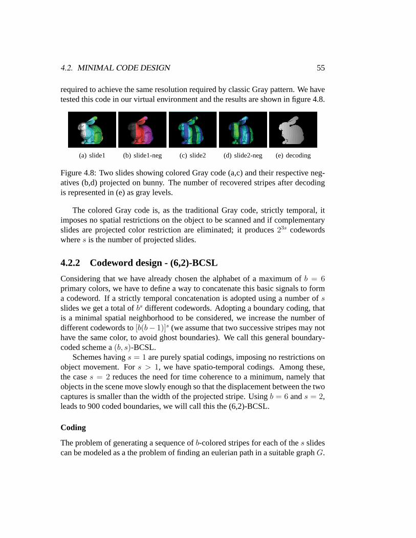
4.2. MINIMAL CODE DESIGN 55
required to achieve the same resolution required by classic Gray pattern. We havetested this code in our virtual environment and the results are shown in figure 4.8.
(a) slide1 (b) slide1-neg (c) slide2 (d) slide2-neg (e) decoding
Figure 4.8: Two slides showing colored Gray code (a,c) and their respective neg-atives (b,d) projected on bunny. The number of recovered stripes after decodingis represented in (e) as gray levels.
The colored Gray code is, as the traditional Gray code, strictly temporal, itimposes no spatial restrictions on the object to be scanned and if complementaryslides are projected color restriction are eliminated; it produces23s codewordswheres is the number of projected slides.
4.2.2 Codeword design - (6,2)-BCSL
Considering that we have already chosen the alphabet of a maximum ofb = 6primary colors, we have to define a way to concatenate this basic signals to forma codeword. If a strictly temporal concatenation is adopted using a number ofsslides we get a total ofbs different codewords. Adopting a boundary coding, thatis a minimal spatial neighborhood to be considered, we increase the number ofdifferent codewords to[b(b− 1)]s (we assume that two successive stripes may nothave the same color, to avoid ghost boundaries). We call this general boundary-coded scheme a(b, s)-BCSL.
Schemes havings = 1 are purely spatial codings, imposing no restrictions onobject movement. Fors > 1, we have spatio-temporal codings. Among these,the cases = 2 reduces the need for time coherence to a minimum, namely thatobjects in the scene move slowly enough so that the displacement between the twocaptures is smaller than the width of the projected stripe. Usingb = 6 ands = 2,leads to 900 coded boundaries, we will call this the (6,2)-BCSL.
Coding
The problem of generating a sequence ofb-colored stripes for each of thes slidescan be modeled as a the problem of finding an eulerian path in a suitable graphG.
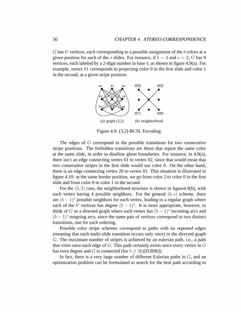
56 CHAPTER 4. STEREO CORRESPONDENCE
G hasbs vertices, each corresponding to a possible assignment of theb colors at agiven position for each of thes slides. For instance, ifb = 3 ands = 2, G has 9vertices, each labeled by a 2-digit number in baseb, as shown in figure 4.9(a). Forexample, vertex01 corresponds to projecting color 0 in the first slide and color 1in the second, at a given stripe position.
(a) graph (3,2) (b) neighborhood
Figure 4.9: (3,2)-BCSL Encoding.
The edges ofG correspond to the possible transitions for two consecutivestripe positions. The forbidden transitions are those that repeat the same colorat the same slide, in order to disallow ghost boundaries. For instance, in 4.9(a),there isn’t an edge connecting vertex 01 to vertex 02, since that would mean thattwo consecutive stripes in the first slide would use color 0. On the other hand,there is an edge connecting vertex 20 to vertex 01. This situation is illustrated infigure 4.10: at the same border position, we go from color 2 to color 0 in the firstslide and from color 0 to color 1 in the second.
For the(3, 2) case, the neighborhood structure is shown in figure4.9(b), witheach vertex having 4 possible neighbors. For the general(b, s) scheme, thereare(b − 1)s possible neighbors for each vertex, leading to a regular graph whereeach of thebs vertices has degree(b − 1)s. It is more appropriate, however, tothink of G as a directed graph where each vertex has(b − 1)s incoming arcs and(b − 1)s outgoing arcs, since the same pair of vertices correspond to two distincttransitions, one for each ordering.
Possible color stripe schemes correspond to paths with no repeated edges(meaning that each multi-slide transition occurs only once) in the directed graphG. The maximum number of stripes is achieved by an eulerian path, i.e., a paththat visits once each edge ofG. This path certainly exists since every vertex inGhas even degree andG is connected (forb ≥ 3) ([D.B96]).
In fact, there is a very large number of different Eulerian paths inG, and anoptimization problem can be formulated to search for the best path according to
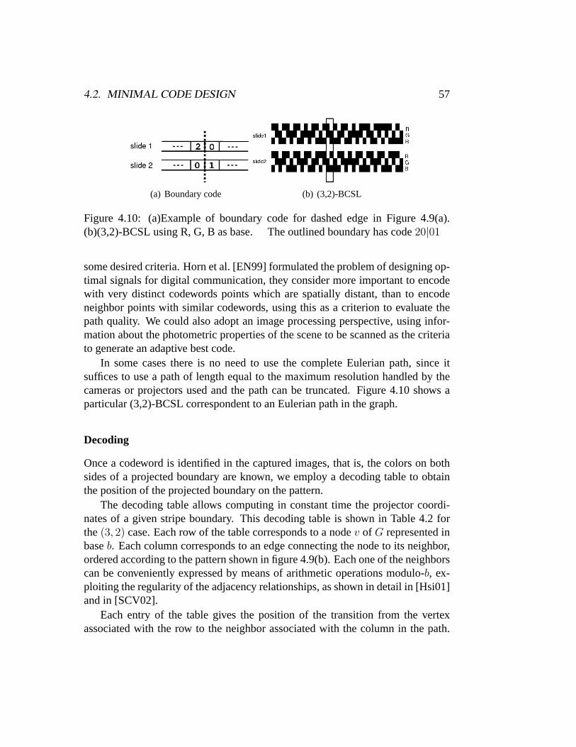
4.2. MINIMAL CODE DESIGN 57
(a) Boundary code (b) (3,2)-BCSL
Figure 4.10: (a)Example of boundary code for dashed edge in Figure 4.9(a).(b)(3,2)-BCSL using R, G, B as base. The outlined boundary has code20|01
some desired criteria. Horn et al. [EN99] formulated the problem of designing op-timal signals for digital communication, they consider more important to encodewith very distinct codewords points which are spatially distant, than to encodeneighbor points with similar codewords, using this as a criterion to evaluate thepath quality. We could also adopt an image processing perspective, using infor-mation about the photometric properties of the scene to be scanned as the criteriato generate an adaptive best code.
In some cases there is no need to use the complete Eulerian path, since itsuffices to use a path of length equal to the maximum resolution handled by thecameras or projectors used and the path can be truncated. Figure 4.10 shows aparticular (3,2)-BCSL correspondent to an Eulerian path in the graph.
Decoding
Once a codeword is identified in the captured images, that is, the colors on bothsides of a projected boundary are known, we employ a decoding table to obtainthe position of the projected boundary on the pattern.
The decoding table allows computing in constant time the projector coordi-nates of a given stripe boundary. This decoding table is shown in Table 4.2 forthe(3, 2) case. Each row of the table corresponds to a nodev of G represented inbaseb. Each column corresponds to an edge connecting the node to its neighbor,ordered according to the pattern shown in figure 4.9(b). Each one of the neighborscan be conveniently expressed by means of arithmetic operations modulo-b, ex-ploiting the regularity of the adjacency relationships, as shown in detail in [Hsi01]and in [SCV02].
Each entry of the table gives the position of the transition from the vertexassociated with the row to the neighbor associated with the column in the path.
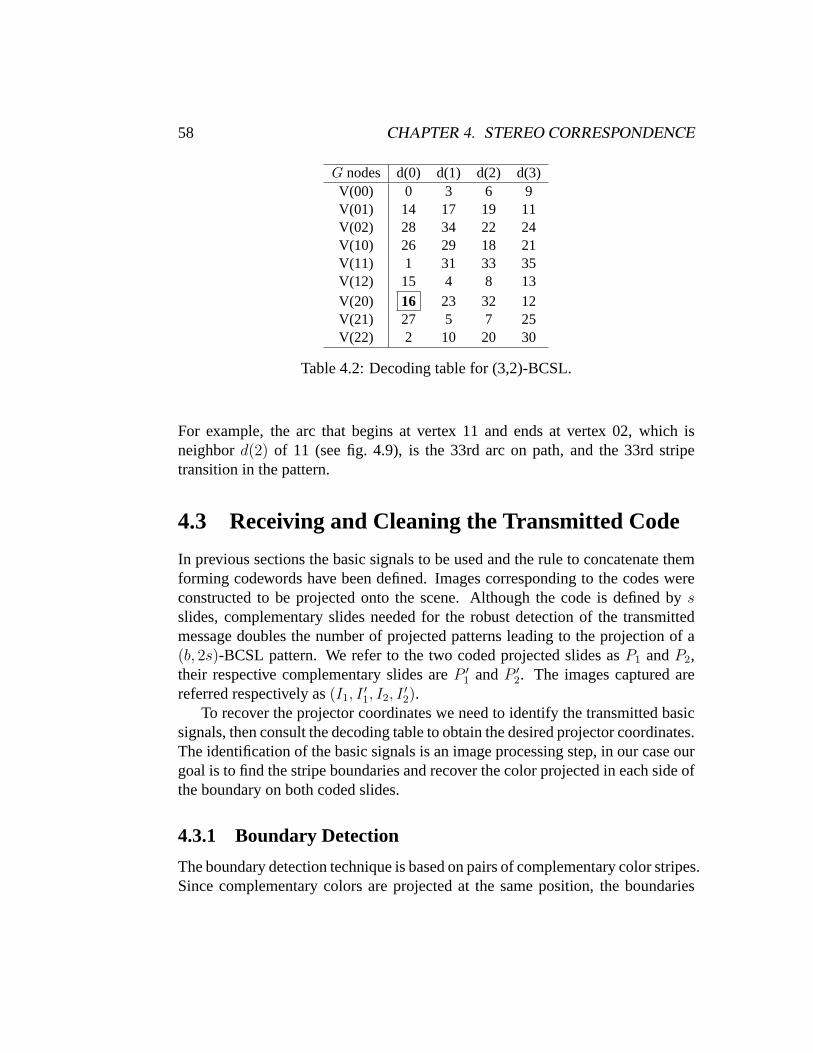
58 CHAPTER 4. STEREO CORRESPONDENCE
G nodes d(0) d(1) d(2) d(3)V(00) 0 3 6 9V(01) 14 17 19 11V(02) 28 34 22 24V(10) 26 29 18 21V(11) 1 31 33 35V(12) 15 4 8 13V(20) 16 23 32 12V(21) 27 5 7 25V(22) 2 10 20 30
Table 4.2: Decoding table for (3,2)-BCSL.
For example, the arc that begins at vertex 11 and ends at vertex 02, which isneighbord(2) of 11 (see fig. 4.9), is the 33rd arc on path, and the 33rd stripetransition in the pattern.
4.3 Receiving and Cleaning the Transmitted Code
In previous sections the basic signals to be used and the rule to concatenate themforming codewords have been defined. Images corresponding to the codes wereconstructed to be projected onto the scene. Although the code is defined bysslides, complementary slides needed for the robust detection of the transmittedmessage doubles the number of projected patterns leading to the projection of a(b, 2s)-BCSL pattern. We refer to the two coded projected slides asP1 andP2,their respective complementary slides areP ′
1 andP ′2. The images captured are
referred respectively as(I1, I′1, I2, I
′2).
To recover the projector coordinates we need to identify the transmitted basicsignals, then consult the decoding table to obtain the desired projector coordinates.The identification of the basic signals is an image processing step, in our case ourgoal is to find the stripe boundaries and recover the color projected in each side ofthe boundary on both coded slides.
4.3.1 Boundary Detection
The boundary detection technique is based on pairs of complementary color stripes.Since complementary colors are projected at the same position, the boundaries
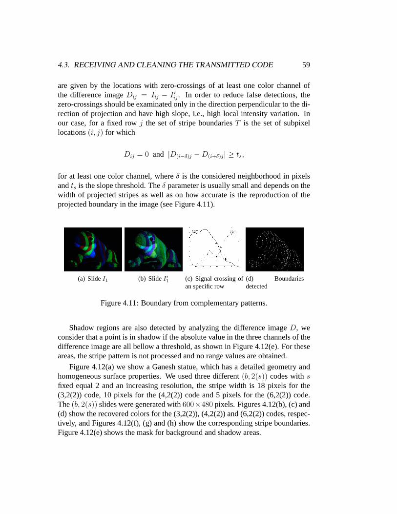
4.3. RECEIVING AND CLEANING THE TRANSMITTED CODE 59
are given by the locations with zero-crossings of at least one color channel ofthe difference imageDij = Iij − I ′ij. In order to reduce false detections, thezero-crossings should be examinated only in the direction perpendicular to the di-rection of projection and have high slope, i.e., high local intensity variation. Inour case, for a fixed rowj the set of stripe boundariesT is the set of subpixellocations(i, j) for which
Dij = 0 and |D(i−δ)j −D(i+δ)j| ≥ ts,
for at least one color channel, whereδ is the considered neighborhood in pixelsandts is the slope threshold. Theδ parameter is usually small and depends on thewidth of projected stripes as well as on how accurate is the reproduction of theprojected boundary in the image (see Figure 4.11).
(a) SlideI1 (b) SlideI ′1 (c) Signal crossing ofan specific row
(d) Boundariesdetected
Figure 4.11: Boundary from complementary patterns.
Shadow regions are also detected by analyzing the difference imageD, weconsider that a point is in shadow if the absolute value in the three channels of thedifference image are all bellow a threshold, as shown in Figure 4.12(e). For theseareas, the stripe pattern is not processed and no range values are obtained.
Figure 4.12(a) we show a Ganesh statue, which has a detailed geometry andhomogeneous surface properties. We used three different(b, 2(s)) codes withsfixed equal 2 and an increasing resolution, the stripe width is 18 pixels for the(3,2(2)) code, 10 pixels for the (4,2(2)) code and 5 pixels for the (6,2(2)) code.The(b, 2(s)) slides were generated with600×480 pixels. Figures 4.12(b), (c) and(d) show the recovered colors for the (3,2(2)), (4,2(2)) and (6,2(2)) codes, respec-tively, and Figures 4.12(f), (g) and (h) show the corresponding stripe boundaries.Figure 4.12(e) shows the mask for background and shadow areas.
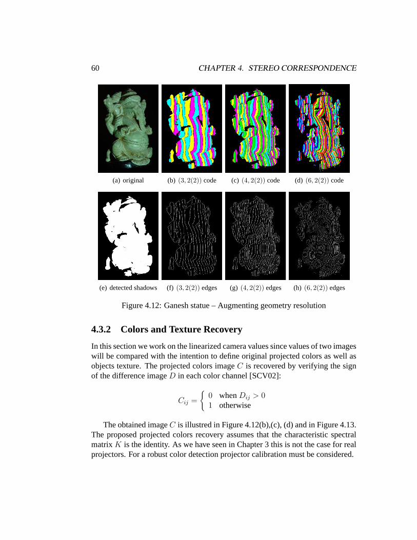
60 CHAPTER 4. STEREO CORRESPONDENCE
(a) original (b) (3, 2(2)) code (c) (4, 2(2)) code (d) (6, 2(2)) code
(e) detected shadows (f) (3, 2(2)) edges (g) (4, 2(2)) edges (h) (6, 2(2)) edges
Figure 4.12: Ganesh statue – Augmenting geometry resolution
4.3.2 Colors and Texture Recovery
In this section we work on the linearized camera values since values of two imageswill be compared with the intention to define original projected colors as well asobjects texture. The projected colors imageC is recovered by verifying the signof the difference imageD in each color channel [SCV02]:
Cij =
0 whenDij > 01 otherwise
The obtained imageC is illustred in Figure 4.12(b),(c), (d) and in Figure 4.13.The proposed projected colors recovery assumes that the characteristic spectralmatrixK is the identity. As we have seen in Chapter 3 this is not the case for realprojectors. For a robust color detection projector calibration must be considered.
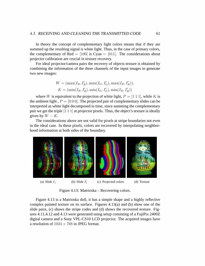
4.3. RECEIVING AND CLEANING THE TRANSMITTED CODE 61
In theory the concept of complementary light colors means that if they aresummed up the resulting signal is white light. Thus, in the case of primary colors,the complementary of Red= [100] is Cyan= [011]. The considerations aboutprojector calibration are crucial in texture recovery.
For ideal projector/camera pairs the recovery of objects texture is obtained bycombining the information of the three channels of the input images to generatetwo new images:
W = (max(IR, I ′R), max(IG, I ′G), max(IB, I ′B)),
K = (min(IR, I ′R), min(IG, I ′G), min(IB, I ′B))
whereW is equivalent to the projection of white light,P = [1 1 1], whileK isthe ambient light ,P = [0 0 0]. The projected pair of complementary slides can beinterpreted as white light decomposed in time, since summing the complementarypair we get the triple[1 1 1] at projector pixels. Thus, the object’s texture is ideallygiven byW −K.
The considerations above are not valid for pixels at stripe boundaries not evenin the ideal case. In these pixels, colors are recovered by interpolating neighbor-hood information at both sides of the boundary.
(a) SlideI1 (b) SlideI ′1 (c) Projected colors (d) Texture
Figure 4.13: Matrioska – Recovering colors.
Figure 4.13 is a Matrioska doll, it has a simple shape and a highly reflectivecomplex painted texture on its surface. Figures 4.13(a) and (b) show one of theslide pairs, (c) shows the stripe codes and (d) shows the recovered texture. Fig-ures 4.11,4.12 and 4.13 were generated using setup consisting of a FujiPix 2400Zdigital camera and a Sony VPL-CS10 LCD projector. The acquired images havea resolution of1024× 768 in JPEG format.
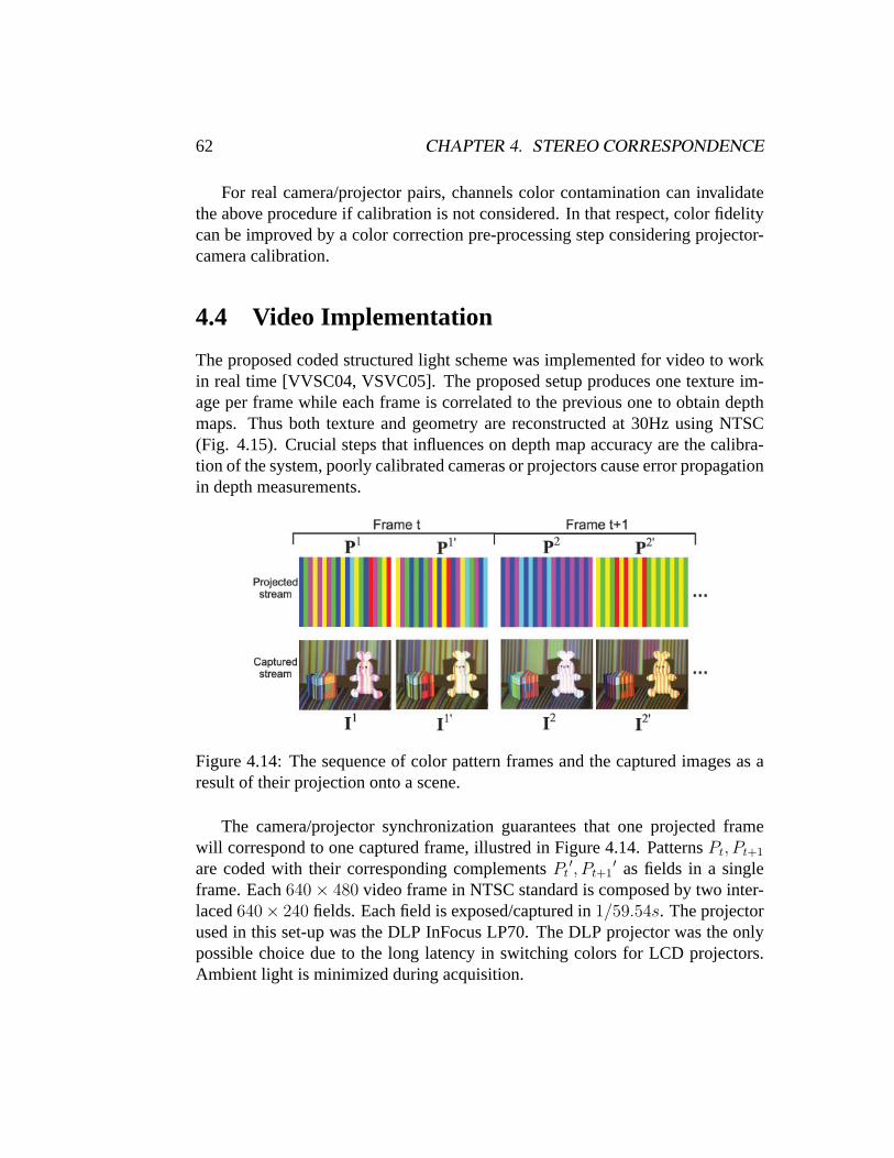
62 CHAPTER 4. STEREO CORRESPONDENCE
For real camera/projector pairs, channels color contamination can invalidatethe above procedure if calibration is not considered. In that respect, color fidelitycan be improved by a color correction pre-processing step considering projector-camera calibration.
4.4 Video Implementation
The proposed coded structured light scheme was implemented for video to workin real time [VVSC04, VSVC05]. The proposed setup produces one texture im-age per frame while each frame is correlated to the previous one to obtain depthmaps. Thus both texture and geometry are reconstructed at 30Hz using NTSC(Fig. 4.15). Crucial steps that influences on depth map accuracy are the calibra-tion of the system, poorly calibrated cameras or projectors cause error propagationin depth measurements.
Figure 4.14: The sequence of color pattern frames and the captured images as aresult of their projection onto a scene.
The camera/projector synchronization guarantees that one projected framewill correspond to one captured frame, illustred in Figure 4.14. PatternsPt, Pt+1
are coded with their corresponding complementsPt′, Pt+1
′ as fields in a singleframe. Each640× 480 video frame in NTSC standard is composed by two inter-laced640× 240 fields. Each field is exposed/captured in1/59.54s. The projectorused in this set-up was the DLP InFocus LP70. The DLP projector was the onlypossible choice due to the long latency in switching colors for LCD projectors.Ambient light is minimized during acquisition.
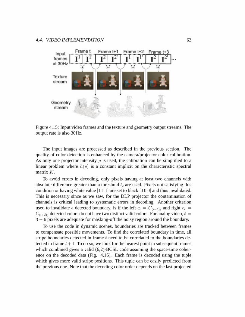
4.4. VIDEO IMPLEMENTATION 63
Figure 4.15: Input video frames and the texture and geometry output streams. Theoutput rate is also 30Hz.
The input images are processed as described in the previous section. Thequality of color detection is enhanced by the camera/projector color calibration.As only one projector intensityρ is used, the calibration can be simplified to alinear problem whereh(ρ) is a constant implicit on the characteristic spectralmatrixK.
To avoid errors in decoding, only pixels having at least two channels withabsolute difference greater than a thresholdtc are used. Pixels not satisfying thiscondition or having white value[1 1 1] are set to black[0 0 0] and thus invalidated.This is necessary since as we saw, for the DLP projector the contamination ofchannels is critical leading to systematic errors in decoding. Another criterionused to invalidate a detected boundary, is if the leftcl = C(i−δ)j and rightcr =C(i+δ)j detected colors do not have two distinct valid colors. For analog video,δ =3− 6 pixels are adequate for masking-off the noisy region around the boundary.
To use the code in dynamic scenes, boundaries are tracked between framesto compensate possible movements. To find the correlated boundary in time, allstripe boundaries detected in framet need to be correlated to the boundaries de-tected in framet+1. To do so, we look for the nearest point in subsequent frameswhich combined gives a valid (6,2)-BCSL code assuming the space-time coher-ence on the decoded data (Fig. 4.16). Each frame is decoded using the tuplewhich gives more valid stripe positions. This tuple can be easily predicted fromthe previous one. Note that the decoding color order depends on the last projected
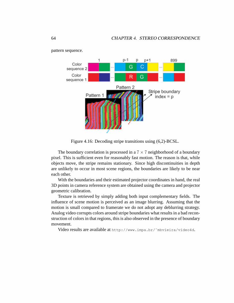
64 CHAPTER 4. STEREO CORRESPONDENCE
pattern sequence.
Figure 4.16: Decoding stripe transitions using (6,2)-BCSL.
The boundary correlation is processed in a7× 7 neighborhood of a boundarypixel. This is sufficient even for reasonably fast motion. The reason is that, whileobjects move, the stripe remains stationary. Since high discontinuities in depthare unlikely to occur in most scene regions, the boundaries are likely to be neareach other.
With the boundaries and their estimated projector coordinates in hand, the real3D points in camera reference system are obtained using the camera and projectorgeometric calibration.
Texture is retrieved by simply adding both input complementary fields. Theinfluence of scene motion is perceived as an image blurring. Assuming that themotion is small compared to framerate we do not adopt any deblurring strategy.Analog video corrupts colors around stripe boundaries what results in a bad recon-struction of colors in that regions, this is also observed in the presence of boundarymovement.
Video results are available athttp://www.impa.br/˜mbvieira/video4d .
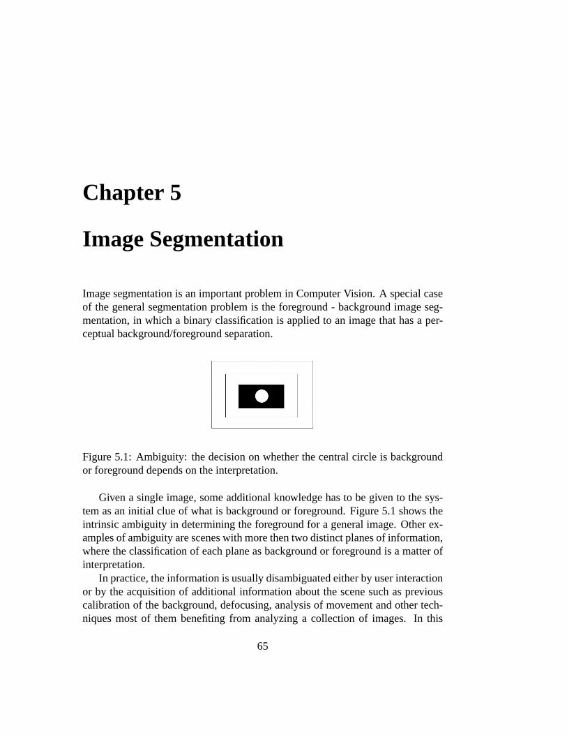
Chapter 5
Image Segmentation
Image segmentation is an important problem in Computer Vision. A special caseof the general segmentation problem is the foreground - background image seg-mentation, in which a binary classification is applied to an image that has a per-ceptual background/foreground separation.
Figure 5.1: Ambiguity: the decision on whether the central circle is backgroundor foreground depends on the interpretation.
Given a single image, some additional knowledge has to be given to the sys-tem as an initial clue of what is background or foreground. Figure 5.1 shows theintrinsic ambiguity in determining the foreground for a general image. Other ex-amples of ambiguity are scenes with more then two distinct planes of information,where the classification of each plane as background or foreground is a matter ofinterpretation.
In practice, the information is usually disambiguated either by user interactionor by the acquisition of additional information about the scene such as previouscalibration of the background, defocusing, analysis of movement and other tech-niques most of them benefiting from analyzing a collection of images. In this
65
66 CHAPTER 5. IMAGE SEGMENTATION
Chapter the active illumination approach is applied to help in the solution of theforeground - background segmentation problem.
5.1 Foreground - Background Segmentation
There are two main branches of research in foreground - background segmenta-tion: one assumes that image acquisition can be controlled to produce images thatare automatically segmented, while the other analyzes a given image without anyassumption about image formation. In the first approach the clues to be analyzedare decided a priori and determine acquisition prerequisites; the segmentation isthen automatic. In the latter the initial clues for solving the problem are insertedby the user a posteriori and no knowledge on acquisition conditions is assumed.One example of a priori information used for foreground segmentation widelyused in practice is chroma key [SB96].
Recently much work has been done in proposing segmentation methods whereclues are inserted a posteriori intending to minimize user intervention. In mostcases the user has to indicate coarsely the foreground and the background pixels[RKB04, WBC∗05] as initial restrictions for a minimization process.
Image Segmentation via graph cut minimization
The image segmentation problem is a special case of a pixel labeling problem. Itcan be modeled as an optimization problem, which consists of computing the bestimage segmentation among all possible image segmentations satisfying a set ofpredefined restrictions.
In pixel labeling problems the goal is to find a labelingf : P 7→ L, mappinga set of pixelsP to a set of labelsL, that minimizes some energy function. Thisenergy function typically has the form
E(f) =∑p∈P
Dp(fp) +∑
p,q∈NVp,q(fp, fq),
whereN ∈ P × P is a neighborhood system onP. Dp(fp) is a functionbased on the observed data that measures the cost of assigning lablefp to p andVp,q(fp, fq) is an spatial smoothness term that measures the cost of assigning labelsfp andfq to adjacent pixelsp andq.
Energy functions likeE are, in general, very difficult to minimize, as they arenon convex functions in large dimensional spaces. When these energy functions

5.2. ACTIVE SEGMENTATION 67
have special characteristics, it is possible to find their exact minimum using dy-namic programming. Nevertheless, in the general case, it is usually necessary torely on general minimization techniques.
Many approaches found in the literature model the problem of image segmen-tation as an energy minimization problem. Recently, Graph-Cut Minimizationbecame widely used in image segmentation [ADA∗04, RKB04, BVZ01].
An interesting property of a graph cutC is that it can be related to a labelingf , mapping the set of verticesV − s, t of a graphG to the set0, 1, wheref(v) = 0, if v ∈ S, andf(v) = 1, if v ∈ T . This labeling defines abinarypartitioningof the vertices of the graph.
The optimality of graph cut minimization methods, considering labeling prob-lems, depends on the number of labels and the exact form of the smoothness termV . In [GPS89]is proved that the method yields global minimum solutions forbinary labeling problem. In [IG98] it is proved that, for labeling problems witharbitrary number of labels, if the smoothness term is restricted to a convex func-tion, it is possible to compute global minima.
In most image segmentation applications, it is desirable to preserve boundarydiscontinuities. This is not possible by using a convex function as the smooth-ness penalty term in the energy function. In general, the minimization for energyfunctions that preserve discontinuities by graph cut minimization can only pro-duce approximate solutions. In [BVZ01] a graph cut based algorithm is proposedthat is able to compute a local minimum for discontinuity preserving energy func-tions. The authors also proved that the obtained local minimum lies within a smallmultiplicative factor(equal to 2) of the global minimum.
The early proposals that used graph cut optimization as a method for energyminimization required the construction of a specific graph for each particularproblem. In [KZ04] is introduced a general scheme for graph cut minimization ofenergy functions that belong to the class of regular functions.
5.2 Active Segmentation
Active illumination can be combined with graph-cut optimization to perform thesegmentation of foreground regions. We call thisactive segmentation, meaningthe use of a light sources to illuminate only the objects to be segmented leavingthe background essentially unchanged. Thus, the light source works as a sub-stitute to the user, acting on the scene to indicate object and background seedelements automatically. This pre-segmentation provides the color distribution of

68 CHAPTER 5. IMAGE SEGMENTATION
each region, that can be used in a graph-cut optimization step to obtain the finalsegmentation.
In recent works, camera flash was explored to enhance image quality. [ED04],[PAH∗04] have proposed the use of bilateral filter to decompose a flash/non-flashpair of images and then recombine them appropriately; both authors have to dealwith shadows produced by the flash. Multiple images with flash positioned indifferent locations among them is used to extract object borders in [RTF∗04] anda non-photorealistic rendering is then applied to the images. Our work differsfrom these previous works since it explores a light source, specially positioned toilluminate only the objects to be segmented, that stays in a fixed position betweenshots.
5.2.1 Active illumination with Graph-Cut Optimization
By modulating segmentation light intensity in subsequent images (by projectingintensityρi) we getIρi
(illustrated in Figure 5.2). We assume that the ambient lightdoes not change between two shots and that all camera parameters are fixed. Sincewe are not actively illuminating the background pixelsp with the segmentationlight source, we haveIλ2(p) ≈ Iλ1(p).
Figure 5.2: (left) and (center) are the input images differently illuminated by vary-ing the camera flash intensity between shots, (right) is the difference thresholdedimage.
The luminance difference is used to build a likelihood function for backgroundmembership. The higher the difference, the lower the likelihood that the pixelbelongs to the background. Thus, pixels for which the luminance difference isgreater than a given threshold are likely to belong to the object and are used todefine the initial seed to the optimization method.
The initial seed gives important clues about the regions that are likely to belongto the background and foreground regions. Based on these clues, it is possible to
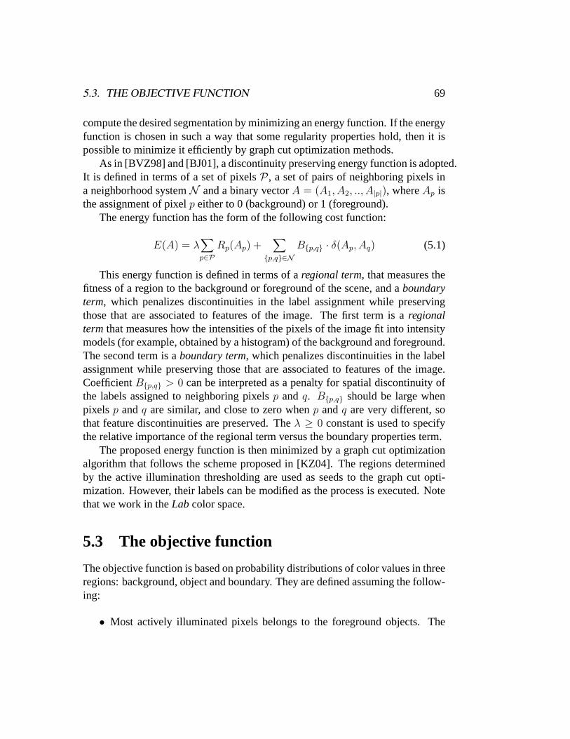
5.3. THE OBJECTIVE FUNCTION 69
compute the desired segmentation by minimizing an energy function. If the energyfunction is chosen in such a way that some regularity properties hold, then it ispossible to minimize it efficiently by graph cut optimization methods.
As in [BVZ98] and [BJ01], a discontinuity preserving energy function is adopted.It is defined in terms of a set of pixelsP, a set of pairs of neighboring pixels ina neighborhood systemN and a binary vectorA = (A1, A2, .., A|p|), whereAp isthe assignment of pixelp either to 0 (background) or 1 (foreground).
The energy function has the form of the following cost function:
E(A) = λ∑p∈P
Rp(Ap) +∑
p,q∈NBp,q · δ(Ap, Aq) (5.1)
This energy function is defined in terms of aregional term, that measures thefitness of a region to the background or foreground of the scene, and aboundaryterm, which penalizes discontinuities in the label assignment while preservingthose that are associated to features of the image. The first term is aregionalterm that measures how the intensities of the pixels of the image fit into intensitymodels (for example, obtained by a histogram) of the background and foreground.The second term is aboundary term, which penalizes discontinuities in the labelassignment while preserving those that are associated to features of the image.CoefficientBp,q > 0 can be interpreted as a penalty for spatial discontinuity ofthe labels assigned to neighboring pixelsp andq. Bp,q should be large whenpixels p andq are similar, and close to zero whenp andq are very different, sothat feature discontinuities are preserved. Theλ ≥ 0 constant is used to specifythe relative importance of the regional term versus the boundary properties term.
The proposed energy function is then minimized by a graph cut optimizationalgorithm that follows the scheme proposed in [KZ04]. The regions determinedby the active illumination thresholding are used as seeds to the graph cut opti-mization. However, their labels can be modified as the process is executed. Notethat we work in theLabcolor space.
5.3 The objective function
The objective function is based on probability distributions of color values in threeregions: background, object and boundary. They are defined assuming the follow-ing:
• Most actively illuminated pixels belongs to the foreground objects. The

70 CHAPTER 5. IMAGE SEGMENTATION
influence of active illumination on the background can lead to wrong overallsegmentation;
• The actively illuminated regions capture the object features, that is, theycontain all color information necessary to distinguish foreground objectsfrom the background;
• Regions corresponding to moving objects in the scene represent a smallfraction of the scene;
• Color differences in Lab space are sufficient to define relevant object - back-ground boundaries.
Figure 5.3: Input images differently illuminated.
The challenge is to define probability distributions that approximate the realdistribution of the expected segmentation regions. For the background region,we employa priori distributions of the luminance differenceLI2 − LI1 . Colorhistograms from the seed regions are used to build a color distribution functionfor the foreground region.
These distributions, together with a boundary likelihood function based ondistances in Lab space, are the basis of the cost function to be proposed.
5.3.1 Composing the cost functions
The goal is to find the labelsX = xp, p ∈ I1, wherexp is 0 if p is backgroundor 1 if p is foreground, that minimize an objective functionE(X). Inspired inInformation Theory, the regional term of the energy function is defined as:
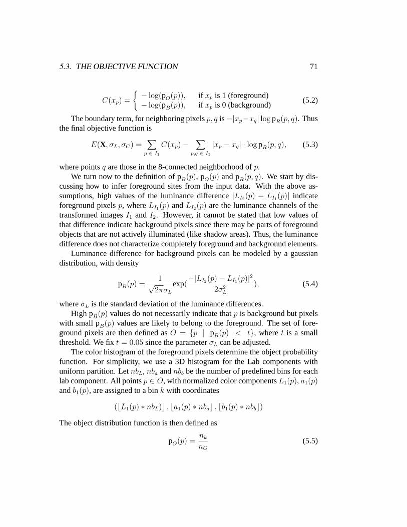
5.3. THE OBJECTIVE FUNCTION 71
C(xp) =
− log(pO(p)), if xp is 1 (foreground)− log(pB(p)), if xp is 0 (background)
(5.2)
The boundary term, for neighboring pixelsp, q is−|xp−xq| log pR(p, q). Thusthe final objective function is
E(X, σL, σC) =∑
p ∈ I1
C(xp)−∑
p,q ∈ I1
|xp − xq| · log pR(p, q), (5.3)
where pointsq are those in the 8-connected neighborhood ofp.We turn now to the definition of pB(p), pO(p) and pR(p, q). We start by dis-
cussing how to infer foreground sites from the input data. With the above as-sumptions, high values of the luminance difference|LI2(p) − LI1(p)| indicateforeground pixelsp, whereLI1(p) andLI2(p) are the luminance channels of thetransformed imagesI1 andI2. However, it cannot be stated that low values ofthat difference indicate background pixels since there may be parts of foregroundobjects that are not actively illuminated (like shadow areas). Thus, the luminancedifference does not characterize completely foreground and background elements.
Luminance difference for background pixels can be modeled by a gaussiandistribution, with density
pB(p) =1√
2πσL
exp(−|LI2(p)− LI1(p)|2
2σ2L
), (5.4)
whereσL is the standard deviation of the luminance differences.High pB(p) values do not necessarily indicate thatp is background but pixels
with small pB(p) values are likely to belong to the foreground. The set of fore-ground pixels are then defined asO = p | pB(p) < t, wheret is a smallthreshold. We fixt = 0.05 since the parameterσL can be adjusted.
The color histogram of the foreground pixels determine the object probabilityfunction. For simplicity, we use a 3D histogram for the Lab components withuniform partition. LetnbL, nba andnbb be the number of predefined bins for eachlab component. All pointsp ∈ O, with normalized color componentsL1(p), a1(p)andb1(p), are assigned to a bink with coordinates
(bL1(p) ∗ nbL)c , ba1(p) ∗ nbac , bb1(p) ∗ nbbc)
The object distribution function is then defined as
pO(p) =nk
nO
(5.5)
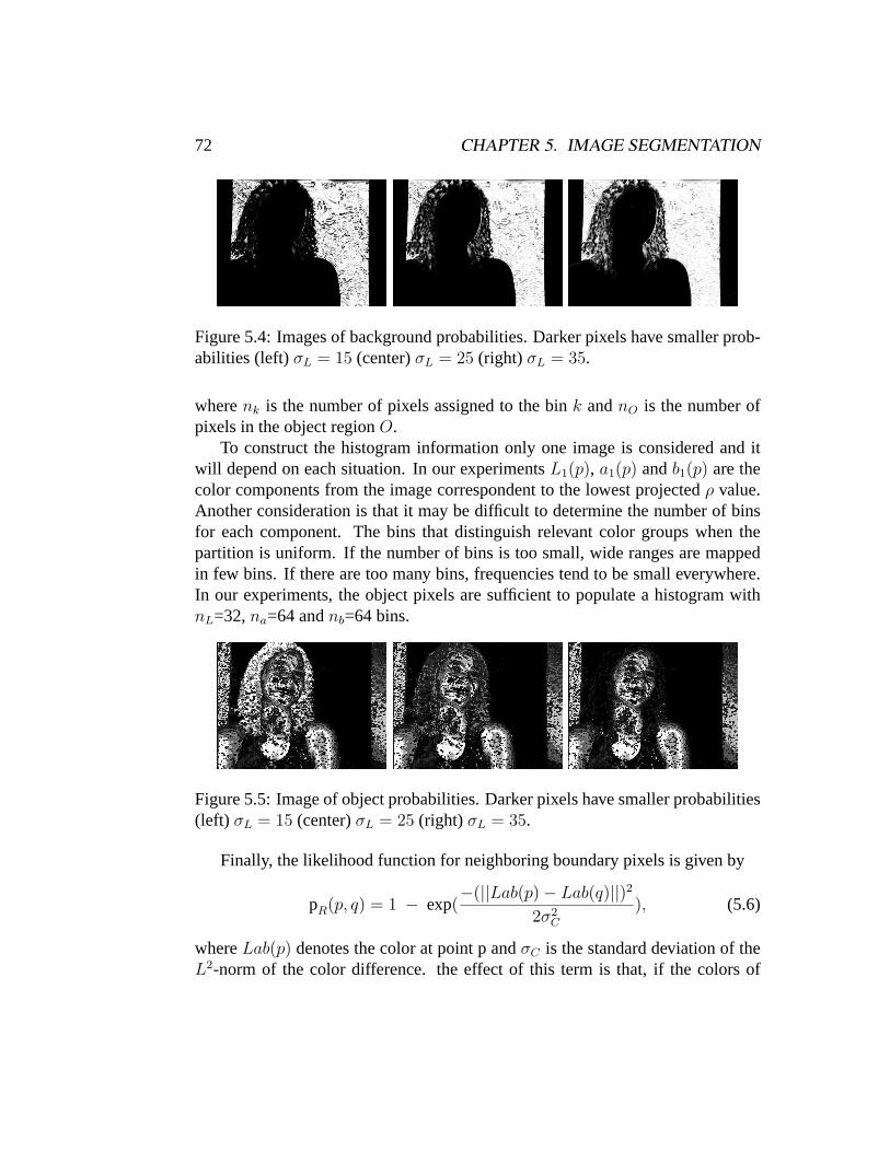
72 CHAPTER 5. IMAGE SEGMENTATION
Figure 5.4: Images of background probabilities. Darker pixels have smaller prob-abilities (left)σL = 15 (center)σL = 25 (right) σL = 35.
wherenk is the number of pixels assigned to the bink andnO is the number ofpixels in the object regionO.
To construct the histogram information only one image is considered and itwill depend on each situation. In our experimentsL1(p), a1(p) andb1(p) are thecolor components from the image correspondent to the lowest projectedρ value.Another consideration is that it may be difficult to determine the number of binsfor each component. The bins that distinguish relevant color groups when thepartition is uniform. If the number of bins is too small, wide ranges are mappedin few bins. If there are too many bins, frequencies tend to be small everywhere.In our experiments, the object pixels are sufficient to populate a histogram withnL=32,na=64 andnb=64 bins.
Figure 5.5: Image of object probabilities. Darker pixels have smaller probabilities(left) σL = 15 (center)σL = 25 (right) σL = 35.
Finally, the likelihood function for neighboring boundary pixels is given by
pR(p, q) = 1 − exp(−(||Lab(p)− Lab(q)||)2
2σ2C
), (5.6)
whereLab(p) denotes the color at point p andσC is the standard deviation of theL2-norm of the color difference. the effect of this term is that, if the colors of
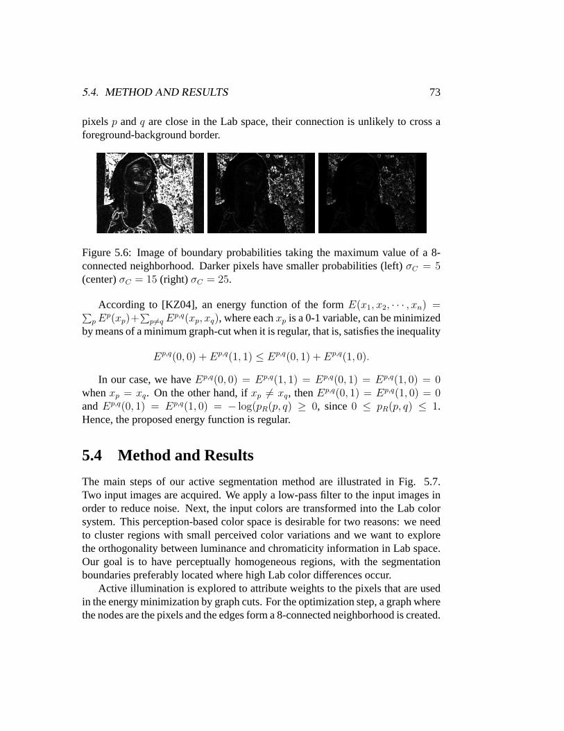
5.4. METHOD AND RESULTS 73
pixelsp andq are close in the Lab space, their connection is unlikely to cross aforeground-background border.
Figure 5.6: Image of boundary probabilities taking the maximum value of a 8-connected neighborhood. Darker pixels have smaller probabilities (left)σC = 5(center)σC = 15 (right) σC = 25.
According to [KZ04], an energy function of the formE(x1, x2, · · · , xn) =∑p Ep(xp)+
∑p6=q Ep,q(xp, xq), where eachxp is a 0-1 variable, can be minimized
by means of a minimum graph-cut when it is regular, that is, satisfies the inequality
Ep,q(0, 0) + Ep,q(1, 1) ≤ Ep,q(0, 1) + Ep,q(1, 0).
In our case, we haveEp,q(0, 0) = Ep,q(1, 1) = Ep,q(0, 1) = Ep,q(1, 0) = 0whenxp = xq. On the other hand, ifxp 6= xq, thenEp,q(0, 1) = Ep,q(1, 0) = 0and Ep,q(0, 1) = Ep,q(1, 0) = − log(pR(p, q) ≥ 0, since0 ≤ pR(p, q) ≤ 1.Hence, the proposed energy function is regular.
5.4 Method and Results
The main steps of our active segmentation method are illustrated in Fig. 5.7.Two input images are acquired. We apply a low-pass filter to the input images inorder to reduce noise. Next, the input colors are transformed into the Lab colorsystem. This perception-based color space is desirable for two reasons: we needto cluster regions with small perceived color variations and we want to explorethe orthogonality between luminance and chromaticity information in Lab space.Our goal is to have perceptually homogeneous regions, with the segmentationboundaries preferably located where high Lab color differences occur.
Active illumination is explored to attribute weights to the pixels that are usedin the energy minimization by graph cuts. For the optimization step, a graph wherethe nodes are the pixels and the edges form a 8-connected neighborhood is created.
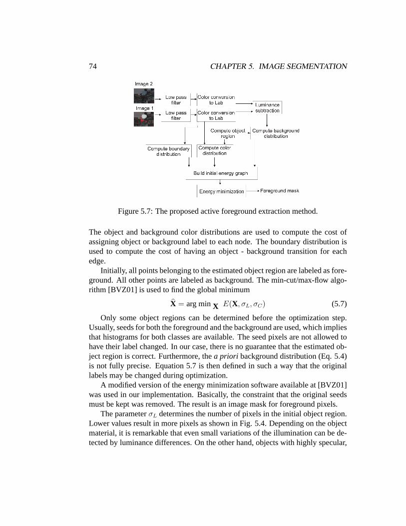
74 CHAPTER 5. IMAGE SEGMENTATION
Figure 5.7: The proposed active foreground extraction method.
The object and background color distributions are used to compute the cost ofassigning object or background label to each node. The boundary distribution isused to compute the cost of having an object - background transition for eachedge.
Initially, all points belonging to the estimated object region are labeled as fore-ground. All other points are labeled as background. The min-cut/max-flow algo-rithm [BVZ01] is used to find the global minimum
X = arg minX E(X, σL, σC) (5.7)
Only some object regions can be determined before the optimization step.Usually, seeds for both the foreground and the background are used, which impliesthat histograms for both classes are available. The seed pixels are not allowed tohave their label changed. In our case, there is no guarantee that the estimated ob-ject region is correct. Furthermore, thea priori background distribution (Eq. 5.4)is not fully precise. Equation 5.7 is then defined in such a way that the originallabels may be changed during optimization.
A modified version of the energy minimization software available at [BVZ01]was used in our implementation. Basically, the constraint that the original seedsmust be kept was removed. The result is an image mask for foreground pixels.
The parameterσL determines the number of pixels in the initial object region.Lower values result in more pixels as shown in Fig. 5.4. Depending on the objectmaterial, it is remarkable that even small variations of the illumination can be de-tected by luminance differences. On the other hand, objects with highly specular,
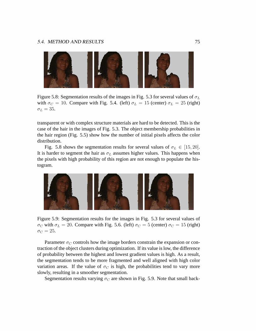
5.4. METHOD AND RESULTS 75
Figure 5.8: Segmentation results of the images in Fig. 5.3 for several values ofσL
with σC = 10. Compare with Fig. 5.4. (left)σL = 15 (center)σL = 25 (right)σL = 35.
transparent or with complex structure materials are hard to be detected. This is thecase of the hair in the images of Fig. 5.3. The object membership probabilities inthe hair region (Fig. 5.5) show how the number of initial pixels affects the colordistribution.
Fig. 5.8 shows the segmentation results for several values ofσL ∈ [15, 20].It is harder to segment the hair asσL assumes higher values. This happens whenthe pixels with high probability of this region are not enough to populate the his-togram.
Figure 5.9: Segmentation results for the images in Fig. 5.3 for several values ofσC with σL = 20. Compare with Fig. 5.6. (left)σC = 5 (center)σC = 15 (right)σC = 25.
ParameterσC controls how the image borders constrain the expansion or con-traction of the object clusters during optimization. If its value is low, the differenceof probability between the highest and lowest gradient values is high. As a result,the segmentation tends to be more fragmented and well aligned with high colorvariation areas. If the value ofσC is high, the probabilities tend to vary moreslowly, resulting in a smoother segmentation.
Segmentation results varyingσC are shown in Fig. 5.9. Note that small back-
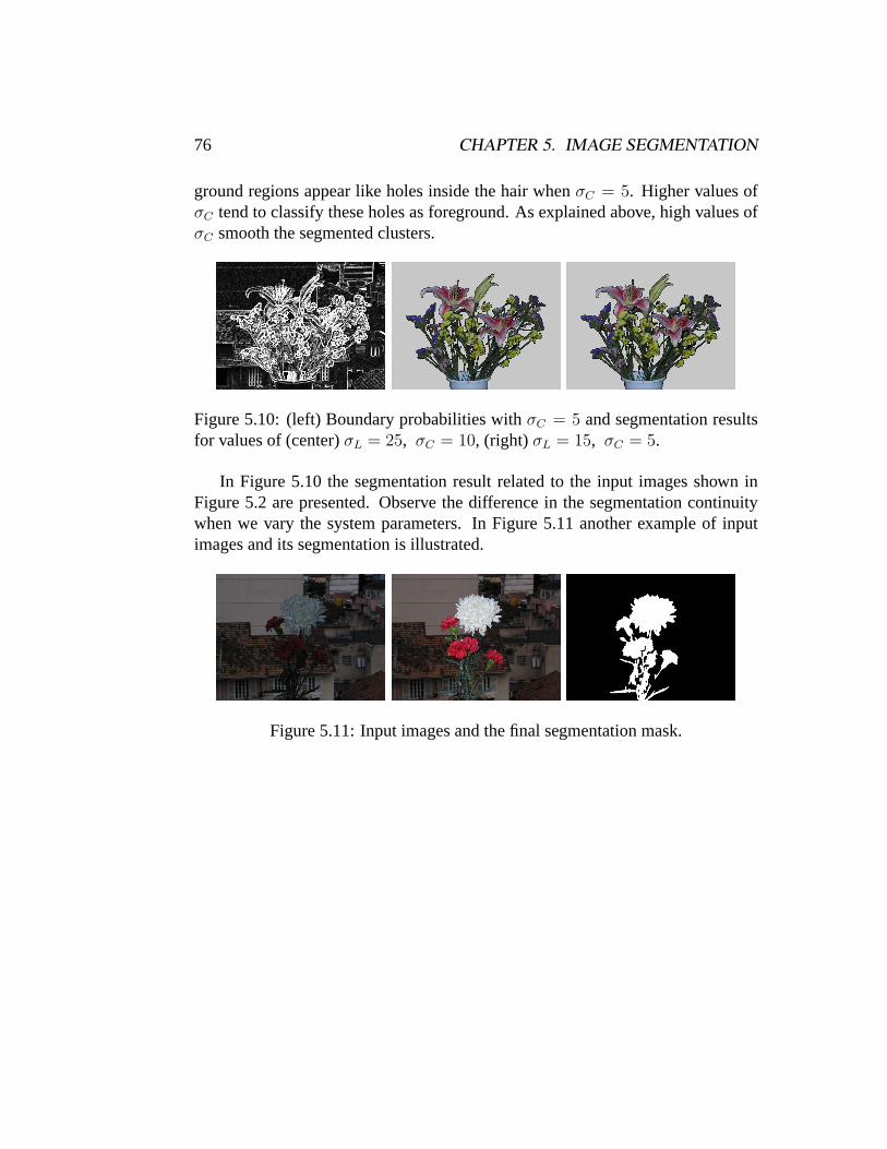
76 CHAPTER 5. IMAGE SEGMENTATION
ground regions appear like holes inside the hair whenσC = 5. Higher values ofσC tend to classify these holes as foreground. As explained above, high values ofσC smooth the segmented clusters.
Figure 5.10: (left) Boundary probabilities withσC = 5 and segmentation resultsfor values of (center)σL = 25, σC = 10, (right) σL = 15, σC = 5.
In Figure 5.10 the segmentation result related to the input images shown inFigure 5.2 are presented. Observe the difference in the segmentation continuitywhen we vary the system parameters. In Figure 5.11 another example of inputimages and its segmentation is illustrated.
Figure 5.11: Input images and the final segmentation mask.
Chapter 6
Tonal Range and Tonal Resolution
In Chapter 2 the camera characteristic response functionf , that characterizes sen-sors behavior respect to pixel exposure values was presented. In Chapter 3,f wasrecovered from a collection of differently exposed images. Thenf−1 was used tolinearize data captured by the camera, as well as to recover real scenes radiancevalues.
In this Chapter, image tonal range and resolution is discussed. The distinctionbetween tonal range and tonal resolution is subtle and it is important to the un-derstanding of some simple operations that can be done to enhance images tonalquality without using the powerful tools of HDR concept. The main question an-swered in this chapter is:What can be done in terms of tonal enhancement of animage without knowledge about the camera characteristicf function and imageradiance values?
We start with a brief review on the recent HDR images research. Then the con-cept of relative tones is introduced and applied to obtain real-time tone enhancedvideo sequences.
6.1 HDRI reconstruction: absolute tones
The research onHigh Dynamic Range Images(HDRI) is looking forward to over-come sensors tonal range limitations. The goal is to achieve better representationand visualization of images, as well as to recover the scenes actual radiance val-ues. We will refer to the scenes radiance values asabsolute tones, since they arerelated to a physical real quantity. The usual images acquired by cameras withlimited dynamic range are theLow Dynamic Range Images(LDRI).
77
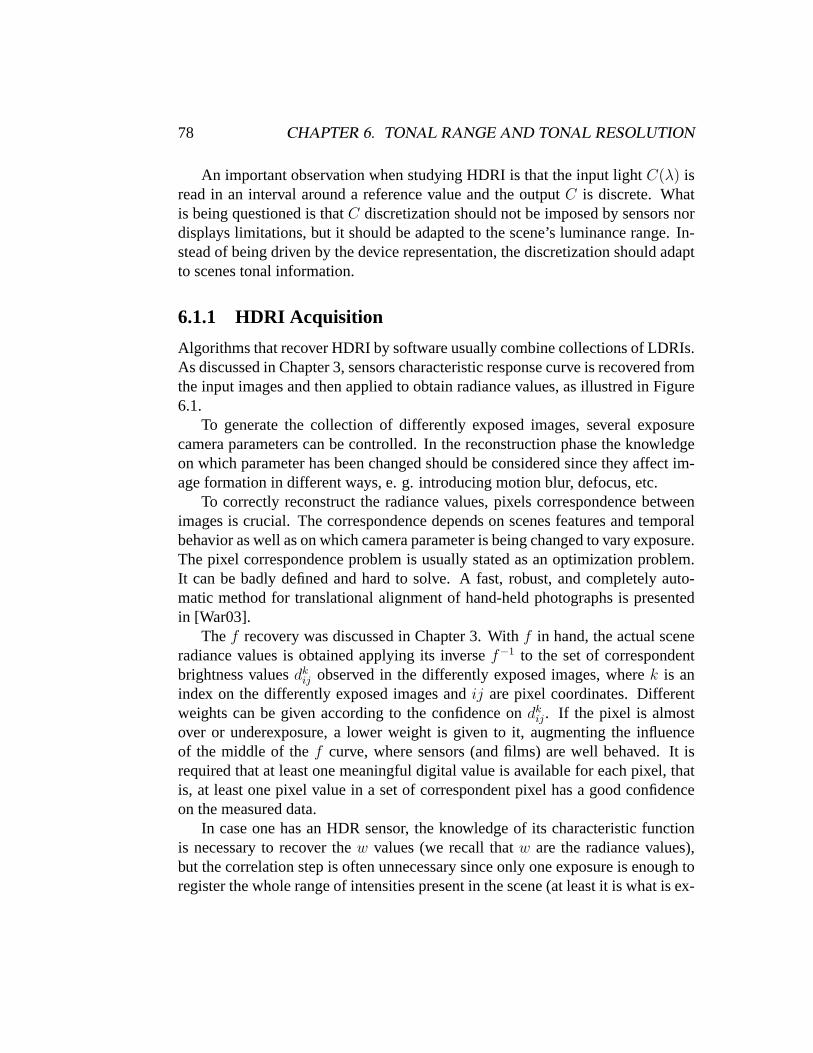
78 CHAPTER 6. TONAL RANGE AND TONAL RESOLUTION
An important observation when studying HDRI is that the input lightC(λ) isread in an interval around a reference value and the outputC is discrete. Whatis being questioned is thatC discretization should not be imposed by sensors nordisplays limitations, but it should be adapted to the scene’s luminance range. In-stead of being driven by the device representation, the discretization should adaptto scenes tonal information.
6.1.1 HDRI Acquisition
Algorithms that recover HDRI by software usually combine collections of LDRIs.As discussed in Chapter 3, sensors characteristic response curve is recovered fromthe input images and then applied to obtain radiance values, as illustred in Figure6.1.
To generate the collection of differently exposed images, several exposurecamera parameters can be controlled. In the reconstruction phase the knowledgeon which parameter has been changed should be considered since they affect im-age formation in different ways, e. g. introducing motion blur, defocus, etc.
To correctly reconstruct the radiance values, pixels correspondence betweenimages is crucial. The correspondence depends on scenes features and temporalbehavior as well as on which camera parameter is being changed to vary exposure.The pixel correspondence problem is usually stated as an optimization problem.It can be badly defined and hard to solve. A fast, robust, and completely auto-matic method for translational alignment of hand-held photographs is presentedin [War03].
Thef recovery was discussed in Chapter 3. Withf in hand, the actual sceneradiance values is obtained applying its inversef−1 to the set of correspondentbrightness valuesdk
ij observed in the differently exposed images, wherek is anindex on the differently exposed images andij are pixel coordinates. Differentweights can be given according to the confidence ondk
ij. If the pixel is almostover or underexposure, a lower weight is given to it, augmenting the influenceof the middle of thef curve, where sensors (and films) are well behaved. It isrequired that at least one meaningful digital value is available for each pixel, thatis, at least one pixel value in a set of correspondent pixel has a good confidenceon the measured data.
In case one has an HDR sensor, the knowledge of its characteristic functionis necessary to recover thew values (we recall thatw are the radiance values),but the correlation step is often unnecessary since only one exposure is enough toregister the whole range of intensities present in the scene (at least it is what is ex-
6.1. HDRI RECONSTRUCTION: ABSOLUTE TONES 79
(a) HDRI recovery (b) Linear TMO (c) Histogram TMO
Figure 6.1: In (a) differently exposed LDR pictures from the same scene are pro-cessed to compose a HDR Radiance Map of the input images. A TMO is thenapplied to visualize the HDR image; figure (b) is visualized using linear TMOand figure (c) using histogram adjustment TMO.
pected from such devices). Scenes of high latitude range can be also syntheticallygenerated by physically-based renderers like RADIANCE [War94].
6.1.2 HDRI Visualization
Usually HDR data is to be visualized on low dynamic range displays. The reduc-tion of the range of image radiances to display brightness in a visual meaningfulway is known as the tone mapping problem. Tone Mapping Operators (TMO)have been firstly proposed to solve the problem of visualization of synthetic im-ages generated by physically based renderers before HDR from photographs be-came popular [LRP97].
In [DCWP02] the tone mapping research is reviewed and TMOs are classifiedin three main classes:spatially uniform time independent, spatially uniform timedependentandspatially varying time independentoperators. Another survey inTMO research is [MNP97]. Recently, specific TMOs for HDR video visualizationhas been proposed. Below, some simple TMOs are described as well as the mainreasoning that guides their intuition.
• Linear Mapping: the simplest way to reduce the range of an HDRI is by
80 CHAPTER 6. TONAL RANGE AND TONAL RESOLUTION
using linear tone mapping, obtained as follows:
d = (w−wmin)Rw
Rd + dmin (6.1)
whereRw = (wmax − wmin)andRd = (dmax − dmin).
• Histogram Adjustment: in [LRP97] is proposed the histogram adjustmentheuristic, it is inspired on the fact that in typical scenes luminance levelsoccur in clusters rather than being uniformly distributed throughout the dy-namic range. The algorithm proposed is:
d = P (w)Rd + dmin (6.2)
where
P (Bw) =[∑
bi<wh(bi)]
[∑
bi<wmaxh(bi)]
= H(w)H(wmax)
(6.3)
• Imaging system simulation: techniques adopted in photographic printingprocess are a source of inspiration to create TMOs. A possible approachis the application of an specific film characteristic curve intending to sim-ulate its look. More complex systems can also be simulated consideringfilm development and enlargement techniques used in photographic labora-tory and they are a source of inspiration to create TMOs, for instance, see[RSSF02, GM03, TR93].
• Human eye simulation: the behavior of human vision is not the same forall illumination conditions, specially in very dim scenes or when there areabrupt illumination changes in time varying scenes. The reality of visu-alized images is achieved only if human vision behavior is modeled. In[LRP97] the histogram adjustment algorithm is extended in many ways tomodel human vision. Also in [THG99] this approach is explored.
In Figure 6.1 the difference of image visualisation depending on the chosenTMO is illustred; after reconstruct the church HDR image, linear TMO was ap-plied to visualize (b) and histogram adjustment was used to visualize (c). Compar-ison between TMOs is mainly perceptual, see [DMMS02]. In [Mac01] perceptionbased image quality metrics are presented.
6.1. HDRI RECONSTRUCTION: ABSOLUTE TONES 81
The Tone Mapping problem can be thought in image color domain as the prob-lem of adjusting the range of image luminances to display luminances maintain-ing color chrominances. Thus it is a quantization problem in radiance domain andTMOs available in literature can be interpreted from this point of view. The uni-form quantization algorithm is comparable to linear TMO, the populosity quan-tization is similar to histogram adjustment. Reasoning like that, a family of newTMOs derived from quantization algorithms can be proposed. The main differ-ence between color quantization and tone mapping is that human eye is moresensitive to spatial changes in luminances than in color. This explains the focus ofseveral TMOs in working on spatial domain, like in human eye perception simu-lation and in dodging-and-burning [RSSF02].
Another branch of research in HDRI visualisation is on HDR displays that areable to represent all tones encoded in an HDR file format [SHS∗04].
6.1.3 HDRI Encoding
HDR data requires accurate tonal representation. Since the digital format can onlyencode discrete quantities, quantization is inevitable, the key point is to control theerror of a high range of values. By simply using more bits to encode pixel valuesthe number of possibly represented tones augment, however, such option can behighly inefficient.
The two approaches used to efficiently represent radiance data are floatingpoint encoding and Log encoding. In floating point encoding a valuev is repre-sented using exponential notation asx · 2y, with x being the mantissa andy theexponent. In Log encoding a valuev is represented asa · ( b
a)v, with a andb being
the minimum and maximum values of the output range. The Log encoding repre-sentation is naturally correlated to the notation of stops and density values widelyused in photography.
The error introduced by encoding in the two cases is different. It is easy to seethat adjacent values in the Log encoding differ by( b
a)N , whereN is the number
of quantization steps of the discretization. Therefore, the quantization error isconstant throughout the whole range. This is in contrast with the floating pointencoding, which does not have equal step sizes.
A very comprehensive analysis of image encodings for HDR Images is avail-able athttp://www.anyhere.com/gward/hdrenc/hdr_encodings.html . Themain HDRI available formats are: the Radiance RGBE, SGI LogLuv, ILM’sOpenEXR and the scRGB encoding.
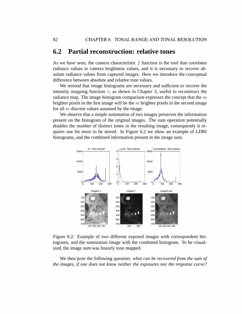
82 CHAPTER 6. TONAL RANGE AND TONAL RESOLUTION
6.2 Partial reconstruction: relative tones
As we have seen, the camera characteristicf function is the tool that correlatesradiance values to camera brightness values, and it is necessary to recover ab-solute radiance values from captured images. Here we introduce the conceptualdifference between absolute and relative tone values.
We remind that image histograms are necessary and sufficient to recover theintensity mapping functionτ , as shown in Chapter 3, useful to reconstruct theradiance map. The image histogram comparison expresses the concept that thembrighter pixels in the first image will be them brighter pixels in the second imagefor all m discrete values assumed by the image.
We observe that a simple summation of two images preserves the informationpresent on the histogram of the original images. The sum operation potentiallydoubles the number of distinct tones in the resulting image, consequently it re-quires one bit more to be stored. In Figure 6.2 we show an example of LDRIhistograms, and the combined information present in the image sum.
Figure 6.2: Example of two different exposed images with correspondent his-tograms, and the summation image with the combined histogram. To be visual-ized, the image sum was linearly tone mapped.
We then pose the following question:what can be recovered from the sum ofthe images, if one does not know neither the exposures nor the response curve?
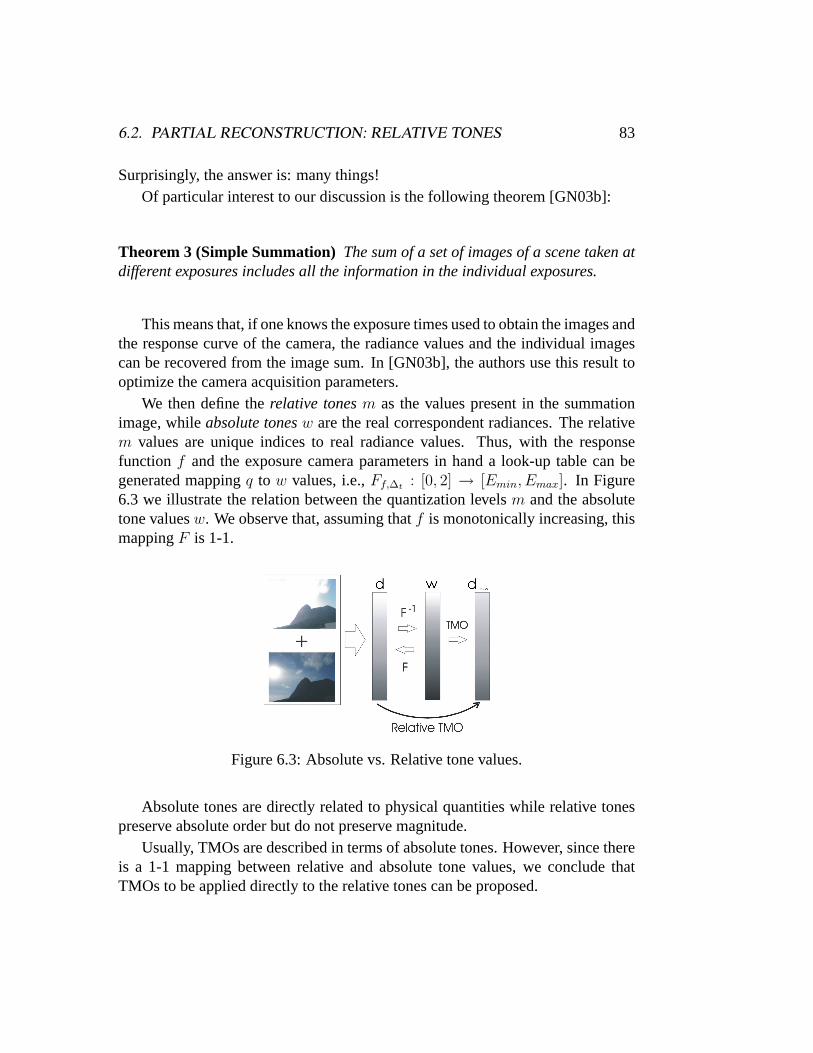
6.2. PARTIAL RECONSTRUCTION: RELATIVE TONES 83
Surprisingly, the answer is: many things!Of particular interest to our discussion is the following theorem [GN03b]:
Theorem 3 (Simple Summation)The sum of a set of images of a scene taken atdifferent exposures includes all the information in the individual exposures.
This means that, if one knows the exposure times used to obtain the images andthe response curve of the camera, the radiance values and the individual imagescan be recovered from the image sum. In [GN03b], the authors use this result tooptimize the camera acquisition parameters.
We then define therelative tonesm as the values present in the summationimage, whileabsolute tonesw are the real correspondent radiances. The relativem values are unique indices to real radiance values. Thus, with the responsefunction f and the exposure camera parameters in hand a look-up table can begenerated mappingq to w values, i.e.,Ff,∆t : [0, 2] → [Emin, Emax]. In Figure6.3 we illustrate the relation between the quantization levelsm and the absolutetone valuesw. We observe that, assuming thatf is monotonically increasing, thismappingF is 1-1.
Figure 6.3: Absolute vs. Relative tone values.
Absolute tones are directly related to physical quantities while relative tonespreserve absolute order but do not preserve magnitude.
Usually, TMOs are described in terms of absolute tones. However, since thereis a 1-1 mapping between relative and absolute tone values, we conclude thatTMOs to be applied directly to the relative tones can be proposed.
84 CHAPTER 6. TONAL RANGE AND TONAL RESOLUTION
6.2.1 Active range-enhancement
When generating differently exposed images, instead of varying the exposuretime, alternative ways to vary pixel exposure can be explored. By controlling lightintensity, while keeping all other camera parameters fixed, the pixel irradiancewij
is altered and hence its correspondent exposure value. This is not usually done,once the illumination intensity varies irregularly throughout the scene. However,the concept of relative tone values introduced here makes possible the use of ac-tive illumination in recovering relative tones to enhance tonal resolution on theactively illuminated area.
Changing light intensity the tonal partial ordering on actively illuminated areasis preserved once reflectance is proportional to incident radiance. Thus, relativetones are naturally recovered by simple summation in those regions.
The fact that illumination mostly affects the foreground pixels can be ex-plored to perform foreground-background segmentation. The algorithm discussedin Chapter 5 can be used to produce a segmentation maskM , where 1 is assignedto the foreground pixels and 0 to the background, defining the actively illuminatedregions.
Using active illumination, the foreground objects not only can be extracted butalso can be tone-enhanced using relative tones concept. Note that the backgroundcannot be tone-enhanced since there is no exposure variation in these regions.The summation image is given byS(dij) = L(dij) + L(dij), with S(dij) ∈ [0, 2].As exposure values are different in two subsequent images tonal resolution is en-hanced by simple summation.
To visualize the foreground tones Larson’s histogram adjustment is applied,TMOsv : [0, 2] → [0, 1], to the actively illuminated region. Chromaticities ofboth images are linearly combined to attenuate problems in over or under-exposedpixels.
The final image is obtained by a simple image composition:
Cij = MijFij + (1−Mij)Bij
WhereFij are the tone-enhanced foreground pixels andBij the background pixelsthat remain unchanged. A low-pass filter is applied to imageM to avoid theperception of discontinuities in transition of segmented regions.
All discussion above assumes that one knows the pixel correspondence in dif-ferently exposed images. This is trivial for static scenes captured by camerasmounted on a tripod. For moving scenes, pixel correspondence has to be solvedbefore applying the method outlined above.

6.3. REAL-TIME TONE-ENHANCED VIDEO 85
6.3 Real-time Tone-Enhanced Video
For video implementation, a set-up composed by a video camera synchronizedwith a projector is used. A video signal, where each field has constant gray colorvaluesρ1 andρ2 with ρ1 6= ρ2 is projected onto the scene. This signal is connectedto the cameragen-lock pin, which guarantees projection/capture synchronization.Each light exposure lasts for1/59.54s using the NTSC standard. The fieldsI1
andI2 of each captured frame represent the same object illuminated differently.This is sufficient for actively segment and tone-enhance the image pair.
Figure 6.4: Two consecutive input fields result in one frame.
Input video images are in the Yuv color space. Thus, the processing is per-formed using the luminance defined asL(pij) = Y (dij), where Y is the videoluminance channel. In this scheme, the tone-enhancement can be applied to anytwo consecutive fields. This produces an output video stream with the same inputframerate, as shown in Fig. 6.4.
We assume that the framerate is high compared to the object’s movement, thus,the effects of moving objects are small between a pair of fields. In the segmenta-tion step, graph-cuts optimization is not applied, only the initial seed is used. Tominimize undesirable effects of shadow regions, the projector is positioned veryclose to the camera. This implies that background should be far enough to notbe affected by active illumination. The working volume can be determined byanalyzing the projector intensity decay with distance (see Chapter 3).
Figures 6.5, 6.6 and 6.7 shows two consecutive video fields with different il-lumination, and their respective resulting tone enhancemed foreground. The pro-jected gray values used wereρ1 = 0.35 andρ2 = 1. The luminance thresholdLmin used is 0.08. One can notice that our method has some trouble segment-ing low-reflectance objects, such as hair. However, the resulting tone-enhancedimages are still quite satisfactory.
A home made cheap version of the system was also implemented, it is com-posed by a web-cam synchronized with a CRT monitor playing the role of activeilluminant. Some results are available athttp://www.impa.br/˜asla/ahdr .

86 CHAPTER 6. TONAL RANGE AND TONAL RESOLUTION
(a) (b) (c)
Figure 6.5: Images (a) and (b) are the video input fields, while in (c) it is shownthe tonal-enhanced foreground.
(a) (b) (c)
Figure 6.6: Images (a) and (b) are the video input fields, while in (c) it is shownthe tonal-enhanced foreground.
(a) (b) (c)
Figure 6.7: Images (a) and (b) are the video input fields, while in (c) it is shownthe tonal-enhanced foreground.
Chapter 7
Conclusion
This work was guided by the concept of active illumination, that was applied inseveral different contexts. The first problem that we have tackled was coded struc-tured light methods for 3D photography purposes. We revisited the usage of colorin code design and proposed a new minimal coding scheme. We also simplifiedthe classification of structured light coding strategies proposed in [JPB04].
In this context, spatial variation of projected light is required, and hence, digi-tal projectors are conveniently adopted as the active light source. The basic setupfor structured light is a camera synchronized with a digital projector.
The proposed coding scheme was implemented for video and it is capableof acquiring depth maps together with scene colors at 30Hz using NTSC-basedhardware. As a consequence of acquisition of both geometry and texture from thesame data, the texture-geometry registration problem is avoided.
During the implementation of the video setup we observed that the hardwareused to project slides and capture images has a direct influence on measurementaccuracy. In a more subtle way, scene illumination conditions and the object’ssurface features also play an important role.
A crucial step that influences on depth map accuracy is the calibration ofthe system: poorly calibrated cameras or projectors cause error propagation indepth measurements. Unappropriate camera models (for instance, using a pin-hole model when lens distortion is relevant) can also generate systematic errors.
We also concluded that the camera/projector photometric calibration is ofgreat importance and that, if not applied, it may lead to decoding failures. Wethen studied more deeply the photometric calibration problem and proposed aprocedure to calibrate the projector relatively to the camera used in the setup.There is still a lot to learn about projectors’ photometric calibration, but we were
87
88 CHAPTER 7. CONCLUSION
able to formalize the problem, proposing a non-linear model to determine both theprojectorspectral characteristic matrixand itscharacteristic emitting function.
Once the active setup was disponible and working for the depth recovery ap-plication, we started to explore other applications of the same setup. In partic-ular, we propose to use active intensity variation for two different applications:background/foreground segmentation and, using the introduced concept of rela-tive tones, image tone-enhancement.
The segmentation method is based on active illumination and employs graph-cut optimization to enhance the inition foreground mask obtained exploring theactive illumination.
The key idea exploited in our method is that light variations can be designedto affect objects that are closer to the camera. In this way, a scene is lit withtwo different intensities of an additional light source that we callsegmentationlight source. By capturing a pair of images with such illumination, we are able todistinguish between objects in the foreground and the scene background.
Several light sources and different illumination schemes can be used to markthe foreground. The proposed method is fully automatic and does not require userintervention to label the image. Moreover, the energy function has only two pa-rameters that must be specified: the standard-deviations of the normal backgroundand boundary distributions. These parameters can be tuned only once for a widevariety of images with similar light setup.
The main technical contributions of this work are the concept of foreground/ background segmentation by active lighting and the design of a suitable energyfunction to be used in the graph-cut minimization.
The quality of the masks produced by our method is, in general, quite good.Some difficult cases may arise when the objects are highly specular, translucentor have very low reflectance. Because of its characteristics, this method is wellsuited for applications in which the user can control the scene illumination; forexample, in studio situations and/or using a flash/no-flash setup.
This method can be naturally extended to active segmentation of video se-quences. All that it is required for this purpose is a synchronized camera/projectorsystem.
Joining HDR images concepts with active light intensity variation we got aouthird application: the image tone-enhancement. The additional information result-ing from capturing two images of the same scene was used to extend the dynamicrange and the tonal resolution of the final image. This technique is made possibleby the concept of relative tone values introduced in this work. We remark thatrelative tones is a key concept in HDR theory and has many other applications,
7.1. FUTURE WORK 89
which we intend to exploit in future work.The synchronized camera and projector setup already implemented was then
adopted to produce tonal-enhanced video. This system has many advantages,such as good cost performance, compatibility and various options of distributionchannels. The data processing of our system can be easily incorporated into thepipeline of a video production environment.
Although our implementation has been done in real time for video, the sameidea could be used in digital cameras, by exploiting flash - no flash photogra-phy. There are many recent works [PAH∗04, ED04] that explore the use of pro-grammable flash to enhance image quality, but they do not use HDR concepts.Our work gives a contribution to this new area of computational photography.
For both applications, segmentation and tone-enhancement, spatial variationof the active light source was not assumed. Therefore, although a digital projec-tor can be used, much simpler controlled light sources can replace the projectorin the implementation of the proposed methods. We have implemented the pro-posed segmentation using intensity variable flashes and a home made setup usinga monitor as light source for tone enhancement.
The main limitation of using active light in different contexts is that the activelight should be the main light source present in the scene or, at least, strong enoughto be distinguished from other light sources. This is a very important considerationwhen planning scene illumination as well as the active light positioning.
7.1 Future Work
As future work we point ou some natural extensions to the proposed applicationsas well as deeper exploitation of projector calibration potentials:
• Model and calibration of radial decay of projector intensity.
• Better decoding and texture recovery by exploring projector calibration toenhance the coded structured-light results.
• Graph-cut segmentation for video, benefiting from temporal coherence ofsubsequent frames; better if working in real time.
• Tone-enhanced matting; better if working in real time.

90 CHAPTER 7. CONCLUSION
Bibliography
[Ada80] ADAMS A.: The Camera, The Ansel Adams Photography series.Little, Brown and Company, 1980.
[Ada81] ADAMS A.: The Negative, The Ansel Adams Photography series.Little, Brown and Company, 1981.
[Ada83] ADAMS A.: The Print, The Ansel Adams Photography series. Little,Brown and Company, 1983.
[ADA ∗04] AGRAWALA A., DONCHEVA M., AGRAWALA M., DRUCKER S.,COLBURN A., CURLESS B., SALESIN D., COHEN M.: Interac-tive digital photomontage. InComputer Graphics Proceedings ACMSIGGRAPH(2004), pp. 294–302.
[BJ01] BOYKOV Y., JOLLY M.: Interactive graph cuts for optimal boundaryand region segmentation of objects in n-d images. InProceedings ofICCV (2001).
[BMS98] BATLLE J., MOUADDIB E., SALVI J.: Recent progress in codedstructured light as a technique to solve the correspondence problem:A survey.Pattern Recognition 31, 7 (1998), 963–982.
[BVZ98] BOYKOV Y., VEKSLER O., ZABIH R.: Markov random fields withefficient approximation. InIEEE Conference on Computer Visionand Pattern Recognition(1998), pp. 648–655.
[BVZ01] BOYKOV Y., VEKSLER O., ZABIH R.: Fast approximate energyminimization via graph cuts.IEEE Transactions on PAMI 23(2001),1222–1239.
91
92 BIBLIOGRAPHY
[CH85] CARRIHILL B., HUMMEL R.: Experiments with the intensity ratiodepth sensor.Comput. Vision Graphics Image Process 32(1985),337–358.
[D.B96] D.B.WEST: Introduction to graph theory. Prentice Hall, 1996.
[DCWP02] DEVLIN K., CHALMERS A., WILKIE A., PURGATHOFERW.: Star:Tone reproduction and physically based spectral rendering. InStateof the Art Reports, Eurographics 2002(September 2002), pp. 101–123.
[DM97] DEBEVEC P., MALIK J.: Recovering high dynamic range radi-ance maps from photographs. InProc. ACM SIGGRAPH ’97(1997),pp. 369–378.
[DMMS02] DRAGO F., MARTENS W., MYSZKOWSKI K., SEIDEL H.: Percep-tual evaluation of tone mapping operators with regard to similarityand preference. InTech. Repport MPI-I-2202-4-002(2002), p. ?
[ED04] EISEMANN E., DURAND F.: Flash photography enhancement via in-trinsic relighting.Computer Graphics Proceedings ACM SIGGRAPH(2004), ?
[EN99] E.HORN, N.KIRYATI : Toward optimal structured light patterns.Im-age and Vision Computing 17, 2 (1999), 87–97.
[GHS01] GOESELE M., HEIDRICH W., SEIDEL H.: Color calibrated highdynamic range imaging with ICC profiles. InProc. of the 9th ColorImaging Conference Color Science and Engineering: Systems, Tech-nologies, Applications, Scottsdale(November 2001), pp. 286–290.
[Gla94] GLASSNERA.: Principles of Digital Image Synthesis. Morgan Kauf-mann Publishers Inc., 1994.
[GM03] GEIGEL J., MUSGRAVE F.: A model for simulating the photo-graphic development process on digital images. InComp. Graph.Proc. (2003), pp. 135–142.
[GN03a] GROSSBERGM., NAYAR S.: Determining the camera response fromimages: What is knowable?IEEE Trans.PAMI 25, 11 (Nov. 2003),1455–1467.
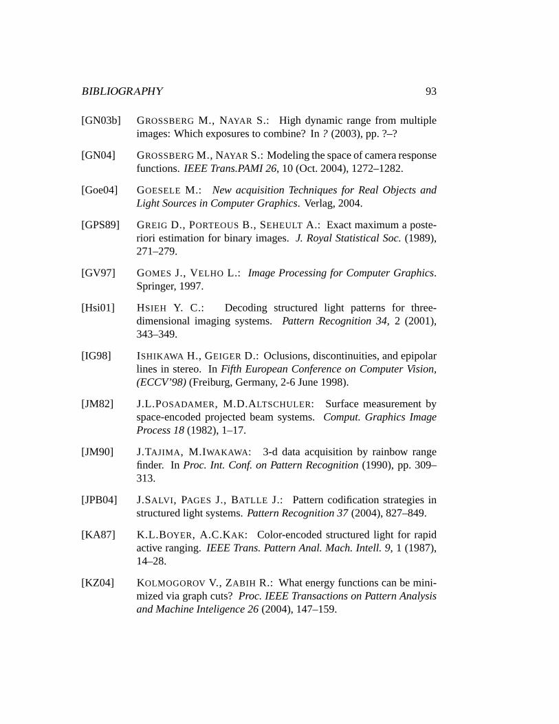
BIBLIOGRAPHY 93
[GN03b] GROSSBERGM., NAYAR S.: High dynamic range from multipleimages: Which exposures to combine? In? (2003), pp. ?–?
[GN04] GROSSBERGM., NAYAR S.: Modeling the space of camera responsefunctions.IEEE Trans.PAMI 26, 10 (Oct. 2004), 1272–1282.
[Goe04] GOESELE M.: New acquisition Techniques for Real Objects andLight Sources in Computer Graphics. Verlag, 2004.
[GPS89] GREIG D., PORTEOUSB., SEHEULT A.: Exact maximum a poste-riori estimation for binary images.J. Royal Statistical Soc.(1989),271–279.
[GV97] GOMES J., VELHO L.: Image Processing for Computer Graphics.Springer, 1997.
[Hsi01] HSIEH Y. C.: Decoding structured light patterns for three-dimensional imaging systems.Pattern Recognition 34, 2 (2001),343–349.
[IG98] ISHIKAWA H., GEIGER D.: Oclusions, discontinuities, and epipolarlines in stereo. InFifth European Conference on Computer Vision,(ECCV’98)(Freiburg, Germany, 2-6 June 1998).
[JM82] J.L.POSADAMER, M.D.ALTSCHULER: Surface measurement byspace-encoded projected beam systems.Comput. Graphics ImageProcess 18(1982), 1–17.
[JM90] J.TAJIMA , M.IWAKAWA : 3-d data acquisition by rainbow rangefinder. InProc. Int. Conf. on Pattern Recognition(1990), pp. 309–313.
[JPB04] J.SALVI , PAGES J., BATLLE J.: Pattern codification strategies instructured light systems.Pattern Recognition 37(2004), 827–849.
[KA87] K.L.B OYER, A.C.KAK : Color-encoded structured light for rapidactive ranging.IEEE Trans. Pattern Anal. Mach. Intell. 9, 1 (1987),14–28.
[KZ04] K OLMOGOROV V., ZABIH R.: What energy functions can be mini-mized via graph cuts?Proc. IEEE Transactions on Pattern Analysisand Machine Inteligence 26(2004), 147–159.
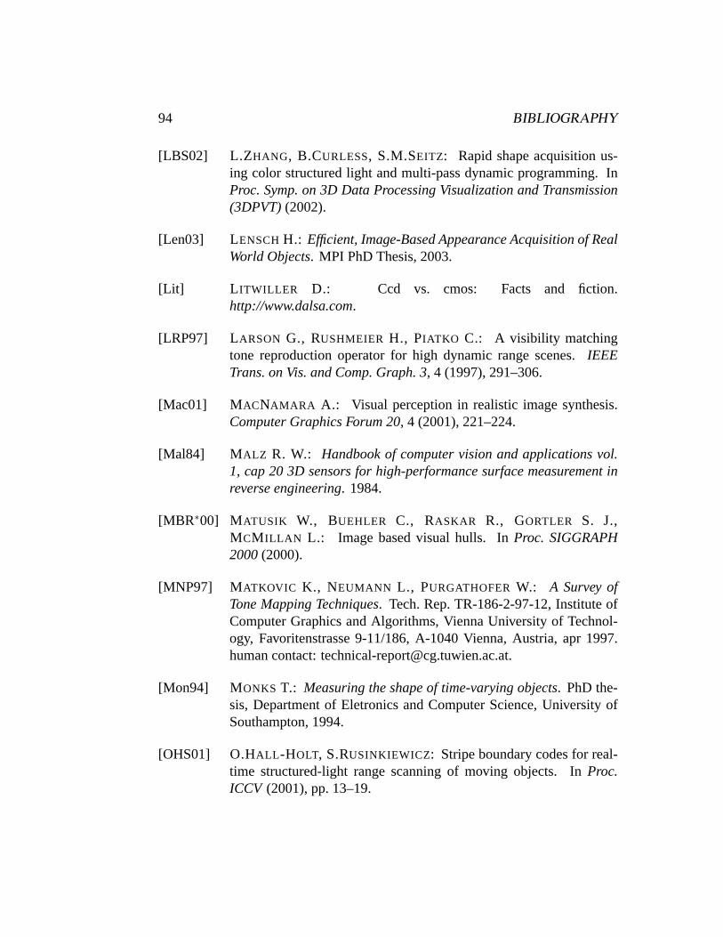
94 BIBLIOGRAPHY
[LBS02] L.ZHANG, B.CURLESS, S.M.SEITZ: Rapid shape acquisition us-ing color structured light and multi-pass dynamic programming. InProc. Symp. on 3D Data Processing Visualization and Transmission(3DPVT)(2002).
[Len03] LENSCHH.: Efficient, Image-Based Appearance Acquisition of RealWorld Objects. MPI PhD Thesis, 2003.
[Lit] L ITWILLER D.: Ccd vs. cmos: Facts and fiction.http://www.dalsa.com.
[LRP97] LARSON G., RUSHMEIER H., PIATKO C.: A visibility matchingtone reproduction operator for high dynamic range scenes.IEEETrans. on Vis. and Comp. Graph. 3, 4 (1997), 291–306.
[Mac01] MACNAMARA A.: Visual perception in realistic image synthesis.Computer Graphics Forum 20, 4 (2001), 221–224.
[Mal84] MALZ R. W.: Handbook of computer vision and applications vol.1, cap 20 3D sensors for high-performance surface measurement inreverse engineering. 1984.
[MBR∗00] MATUSIK W., BUEHLER C., RASKAR R., GORTLER S. J.,MCM ILLAN L.: Image based visual hulls. InProc. SIGGRAPH2000(2000).
[MNP97] MATKOVIC K., NEUMANN L., PURGATHOFER W.: A Survey ofTone Mapping Techniques. Tech. Rep. TR-186-2-97-12, Institute ofComputer Graphics and Algorithms, Vienna University of Technol-ogy, Favoritenstrasse 9-11/186, A-1040 Vienna, Austria, apr 1997.human contact: [email protected].
[Mon94] MONKS T.: Measuring the shape of time-varying objects. PhD the-sis, Department of Eletronics and Computer Science, University ofSouthampton, 1994.
[OHS01] O.HALL -HOLT, S.RUSINKIEWICZ: Stripe boundary codes for real-time structured-light range scanning of moving objects. InProc.ICCV (2001), pp. 13–19.
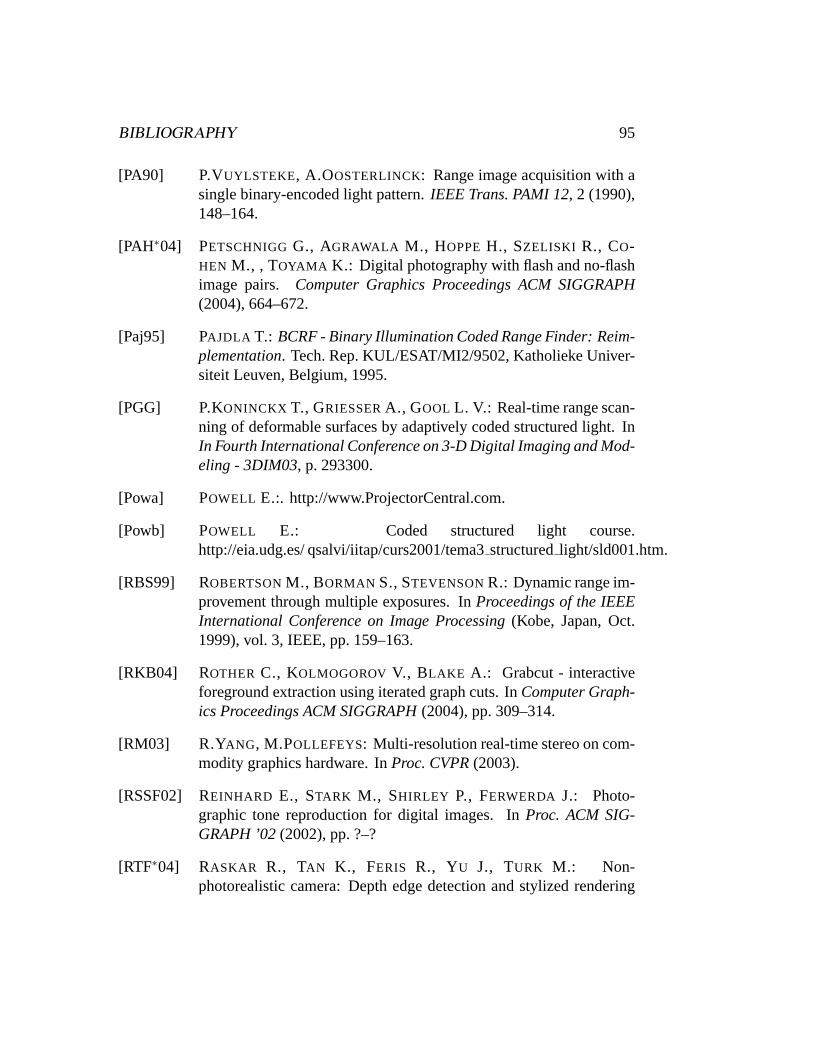
BIBLIOGRAPHY 95
[PA90] P.VUYLSTEKE, A.OOSTERLINCK: Range image acquisition with asingle binary-encoded light pattern.IEEE Trans. PAMI 12, 2 (1990),148–164.
[PAH∗04] PETSCHNIGG G., AGRAWALA M., HOPPEH., SZELISKI R., CO-HEN M., , TOYAMA K.: Digital photography with flash and no-flashimage pairs. Computer Graphics Proceedings ACM SIGGRAPH(2004), 664–672.
[Paj95] PAJDLA T.: BCRF - Binary Illumination Coded Range Finder: Reim-plementation. Tech. Rep. KUL/ESAT/MI2/9502, Katholieke Univer-siteit Leuven, Belgium, 1995.
[PGG] P.KONINCKX T., GRIESSERA., GOOL L. V.: Real-time range scan-ning of deformable surfaces by adaptively coded structured light. InIn Fourth International Conference on 3-D Digital Imaging and Mod-eling - 3DIM03, p. 293300.
[Powa] POWELL E.:. http://www.ProjectorCentral.com.
[Powb] POWELL E.: Coded structured light course.http://eia.udg.es/ qsalvi/iitap/curs2001/tema3structuredlight/sld001.htm.
[RBS99] ROBERTSONM., BORMAN S., STEVENSONR.: Dynamic range im-provement through multiple exposures. InProceedings of the IEEEInternational Conference on Image Processing(Kobe, Japan, Oct.1999), vol. 3, IEEE, pp. 159–163.
[RKB04] ROTHER C., KOLMOGOROV V., BLAKE A.: Grabcut - interactiveforeground extraction using iterated graph cuts. InComputer Graph-ics Proceedings ACM SIGGRAPH(2004), pp. 309–314.
[RM03] R.YANG, M.POLLEFEYS: Multi-resolution real-time stereo on com-modity graphics hardware. InProc. CVPR(2003).
[RSSF02] REINHARD E., STARK M., SHIRLEY P., FERWERDA J.: Photo-graphic tone reproduction for digital images. InProc. ACM SIG-GRAPH ’02(2002), pp. ?–?
[RTF∗04] RASKAR R., TAN K., FERIS R., YU J., TURK M.: Non-photorealistic camera: Depth edge detection and stylized rendering
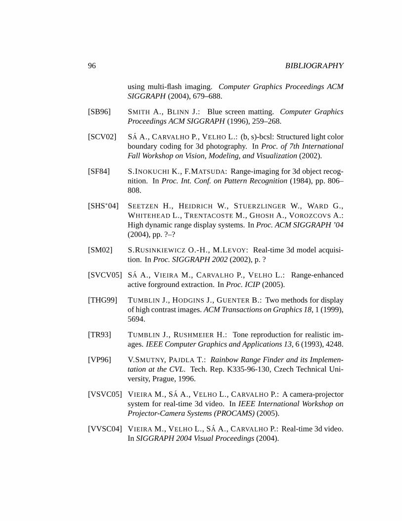
96 BIBLIOGRAPHY
using multi-flash imaging.Computer Graphics Proceedings ACMSIGGRAPH(2004), 679–688.
[SB96] SMITH A., BLINN J.: Blue screen matting.Computer GraphicsProceedings ACM SIGGRAPH(1996), 259–268.
[SCV02] SA A., CARVALHO P., VELHO L.: (b, s)-bcsl: Structured light colorboundary coding for 3d photography. InProc. of 7th InternationalFall Workshop on Vision, Modeling, and Visualization(2002).
[SF84] S.INOKUCHI K., F.MATSUDA: Range-imaging for 3d object recog-nition. In Proc. Int. Conf. on Pattern Recognition(1984), pp. 806–808.
[SHS∗04] SEETZEN H., HEIDRICH W., STUERZLINGER W., WARD G.,WHITEHEAD L., TRENTACOSTEM., GHOSH A., VOROZCOVSA.:High dynamic range display systems. InProc. ACM SIGGRAPH ’04(2004), pp. ?–?
[SM02] S.RUSINKIEWICZ O.-H., M.LEVOY: Real-time 3d model acquisi-tion. In Proc. SIGGRAPH 2002(2002), p. ?
[SVCV05] SA A., V IEIRA M., CARVALHO P., VELHO L.: Range-enhancedactive forground extraction. InProc. ICIP (2005).
[THG99] TUMBLIN J., HODGINS J., GUENTER B.: Two methods for displayof high contrast images.ACM Transactions on Graphics 18, 1 (1999),5694.
[TR93] TUMBLIN J., RUSHMEIER H.: Tone reproduction for realistic im-ages.IEEE Computer Graphics and Applications 13, 6 (1993), 4248.
[VP96] V.SMUTNY, PAJDLA T.: Rainbow Range Finder and its Implemen-tation at the CVL. Tech. Rep. K335-96-130, Czech Technical Uni-versity, Prague, 1996.
[VSVC05] VIEIRA M., SA A., VELHO L., CARVALHO P.: A camera-projectorsystem for real-time 3d video. InIEEE International Workshop onProjector-Camera Systems (PROCAMS)(2005).
[VVSC04] VIEIRA M., VELHO L., SA A., CARVALHO P.: Real-time 3d video.In SIGGRAPH 2004 Visual Proceedings(2004).
BIBLIOGRAPHY 97
[War94] WARD G.: The radiance lighting simulation and rendering system.In Proc. ACM SIGGRAPH ’04(1994), pp. 459–472.
[War03] WARD G.: Fast, robust image registration for compositing high dy-namic range photographcs from hand-held exposures.Journal ofGraphics Tools 8, 2 (2003), 17–30.
[WBC∗05] WANG J., BHAT P., COLBURN R., AGRAWALA M., , COHEN M.:Interactive video cutout.Computer Graphics Proceedings ACM SIG-GRAPH(2005), ?
[ZSCS04] ZHANG L., SNAVELY N., CURLESS B., SEITZ S. M.: Spacetimefaces: high resolution capture for modeling and animation. vol. 23,p. 548558.