Embed Size (px)
Citation preview

University of South FloridaScholar Commons
Graduate Theses and Dissertations Graduate School
4-4-2017
Controlling and Monitoring Voice Quality inInternet CommunicationAn Thanh LeUniversity of South Florida, [email protected]
Follow this and additional works at: http://scholarcommons.usf.edu/etd
Part of the Electrical and Computer Engineering Commons
This Dissertation is brought to you for free and open access by the Graduate School at Scholar Commons. It has been accepted for inclusion inGraduate Theses and Dissertations by an authorized administrator of Scholar Commons. For more information, please [email protected].
Scholar Commons CitationLe, An Thanh, "Controlling and Monitoring Voice Quality in Internet Communication" (2017). Graduate Theses and Dissertations.http://scholarcommons.usf.edu/etd/6659
Controlling and Monitoring Voice Quality in Internet Communication
by
An T. Le
A dissertation submitted in partial fulfillment of the requirements for the degree of
Doctor of Philosophy Department of Electrical Engineering
College of Engineering University of South Florida
Major Professor: Ravi Sankar, Ph.D. Paris Wiley, Ph.D.
Wilfrido A. Moreno, Ph.D. Tapas K. Das, Ph.D.
Richard A. Thompson, Ph.D.
Date of Approval: March 21, 2017
Keywords: Codec, Jitter, Markov, VoIP, Adaptive
Copyright © 2017, An T. Le

DEDICATION
To my teachers, parents, wife, and children
ACKNOWLEDGMENTS
I am truly indebted to my Major Professor, Dr. Ravi Sankar, for his teaching, impeccable
guidance, ceaseless patience, and continued encouragement in last seventeen years and more. I am
deeply grateful to Dr. Richard Thompson, Dr. Paris Wiley, Dr. Wilfrido A. Moreno, and Dr. Tapas
K. Das, for all their technical advice and for serving on my committee.
I would like to sincerely acknowledge the support provided in part by the Florida High
Tech Corridor, Planet Reach, Inc, and voicelabs.org which was instrumental in accomplishing this
dissertation research. Further, I would like to acknowledge the encouragement and help provided
by the iCONS research group members and the Electrical Engineering Department staff in the
College of Engineering, University of South Florida. Finally, without the support of my family,
my wife and children, this dream of pursuing and completing my doctoral degree would not be
possible and even unthinkable.

i
TABLE OF CONTENTS
LIST OF TABLES iv
LIST OF FIGURES v
ABSTRACT vii
CHAPTER 1: INTRODUCTION 1
1.1 Background 1
1.2 Motivation 2
1.3 Research Contributions 3
1.4 Dissertation Structure 3
CHAPTER 2: VOICE OVER INTERNET PROTOCOL 5
2.1 Overview 5
2.2 VoIP Network 6
2.2.1 Review of the Layered Structure of TCP/IP Family 6
2.2.2 Review of the Layered IP Stack 7
2.2.3 VoIP Payload 9
2.2.4 Header Compression 9
2.2.5 VoIP Architecture 9
2.2.6 Soft-switch; Signaling and Payload Transport 10
2.2.7 VoIP in 4G/5G and LTE Communication 11
2.2.8 VoIP with IPv6 11
2.2.9 Summary 11
CHAPTER 3: SPEECH CODEC AND EVALUATION AND SELECTION OF SPEECH CODEC FOR VOIP APPLICATION 13
3.1 Overview 13
3.2 Codec 13
3.2.1 Classification of Speech Codecs 13
3.2.2 Analog – Digital Conversion 14
3.2.3 Waveform CODEC 15
3.2.4 Voice Codec or Vocoder 17
3.2.5 Hybrid Codec 18
3.2.5.1 Regular Pulse Exited Coding 18
3.2.5.2 Multi Pulse Excited Coding 19
3.2.5.3 Code Excited Linear Predictor (CELP) Coders 20
3.2.6 Other Vocoders 22
3.2.6.1 Internet Low Bit-rate Codec (iLBC) 22

ii
3.2.6.2 GIPS 22
3.2.6.3 Speex 23
3.2.6.4 LPC-10 23
3.2.7 Media Format Codecs 24
3.2.8 Codec Loss Concealment Algorithm 24
3.3 Evaluation of Speech Codecs 25
3.3.1 Subjective Measures 25
3.3.2 Objective Measures 26
3.3.2.1 Time-Domain Measures 27
3.3.2.2 Frequency-Domain Measures 28
3.3.2.3 Perceptual Measures 31
3.4 Objective Quality Measures Evaluation 35
3.5 Selection of Speech Codecs 36
3.5.1 Codec Impairment 37
3.5.2 Codec vs. Bandwidth 37
3.5.3 Codec vs. Complexity 39
3.5.4 Codec Selection Based on Implementation Cost 39
3.6 Speech Codec Summary and Future Challenges 39
CHAPTER 4: QUALITY CONTROL AND IMPROVEMENT 41
4.1 Overview 41
4.2 Subjective Measurement 42
4.3 Objective Measurement 42
4.4 Latency, Delay Jitter, and Packet Loss 45
4.4.1 Latency 45
4.4.2 Switching and Queuing 48
4.4.2.1 Packet Switch with Queuing 48
4.4.2.2 Input Queuing and Traffic-handling Capability of an Input-Queued Packet Switch 49
4.4.2.3 Output Queuing 50
4.4.3 Packet Loss 51
4.5 Delay Jitter Measurement 51
4.5.1 Overview 51
4.5.2 Delay Jitter in Packetized Communication 51
4.5.3 Delay Jitter Measurement for Packet without Timestamp 52
4.6 Playout Delay and Markov Model 54
4.6.1 Delay Jitter in VoIP 54
4.6.2 Basics of Fixed and Adaptive Jitter Buffer Models 55
4.7 Fixed Jitter Buffer Application 57
4.8 Self-learning, Adaptive Markov Model Application 57
4.9 Experimental Result for a Simple Playout Delay Scheme 58
4.10 Playout Delay Decision and Analysis Based on Markov Model 61
4.11 Playout Delay Based on Markov Model Experiments 62
4.12 Kalman Filter and Jitter Prediction Improvement 65
CHAPTER 5: SUMMARY AND SUGGESTION FOR FUTURE RESEARCH 66
5.1 Summary 66

iii
5.2 A Maxell Model for Packet Loss Caused by Jitter 67
5.3 VoIP and Social Network 67
5.4 Complex Network and VoIP 67
5.5 Voice in Smart Grid 68
REFERENCES 69
iv
LIST OF TABLES
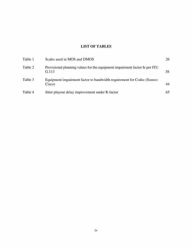
Table 1 Scales used in MOS and DMOS 26
Table 2 Provisional planning values for the equipment impairment factor Ie per ITU G.113 38
Table 3 Equipment impairment factor to bandwidth requirement for Codec (Source: Cisco) 44
Table 4 Jitter playout delay improvement under R-factor 65

v
LIST OF FIGURES
Figure 1 The seven layers of OSI model is stacked into four layers of TCP/IP 6
Figure 2 VoIP protocol stack 7
Figure 3 VoIP header 7
Figure 4 IP header (version 4) 7
Figure 5 IP header (version 6) 8
Figure 6 UDP header (version 4) 8
Figure 7 RTP header (version 4) 8
Figure 8 Overview of VoIP network 10
Figure 9 A simplest waveform-coding scheme 16
Figure 10 PCM coding and PCM word 17
Figure 11 Vocoder block diagram 18
Figure 12 LPC speech synthesizer with multi pulse excitation 20
Figure 13 Analysis-by-synthesis procedure for the multi-pulse excitation 20
Figure 14 CELP encoder 21
Figure 15 CELP decoder 21
Figure 16 Perceptual Audio Quality Measure (PAQM) 34
Figure 17 PSQM calculation procedure 35
Figure 18 Perceived QoS zone 41
Figure 19 An E-model calculation tool 46
Figure 20 Total “mouth to ear” delay in VoIP 47

vi
Figure 21 Perceived voice quality based on network and application performance and channel noise 47
Figure 22 NxN time-slot switch 48
Figure 23 Input queueing switch 49
Figure 24 Input smoothing queued switch 50
Figure 25 Packet voice arriving time 53
Figure 26 Packet loss when no delay plays-out or jitter buffer 55
Figure 27 Play out with a delay or jitter buffer greater than maximum delay jitter 55
Figure 28 Markov model with N states and 3 steps, the probability of transition from state i to state j 58
Figure 29 A simple playout delay scheme using Markov model 59
Figure 30 Delay of a voice channel from Tampa to Los Angeles 59
Figure 31 Quantized delay of a voice channel from Tampa to Los Angeles 60
Figure 32 Transition matrix using two steps Markov model 60
Figure 33 Jitter prediction using Markov model, first step 62
Figure 34 Jitter prediction using Markov model, second step 63
Figure 35 Jitter prediction using Markov model, first step with gain=2 64

vii
ABSTRACT
The Voice over Internet Protocol (VoIP) is on its way to surpassing toll quality. Although
VoIP shares its transmission channel with other communication traffic, today internet has a wider
bandwidth than the legacy Digital Loop Carrier and voice could be digitized higher than traditional
8 kbps, to say 16 kbps. Thus, VoIP should not be limited by the toll quality. However, VoIP
quality could go down, as a result of unpredictable traffic congestion and network imperfections.
These two situations cause delay jitter and packet loss of VoIP. To overcome these challenges,
there are ongoing works for service providers including but not limited to optimizing routing and
adding more bandwidth. There are also works by developers at the user’s end, which includes
compressing voice packet size and processing playout delay adapted to the network condition.
While VoIP planning or off-line quality monitoring and control use overall quality
measurements such as mean opinion score (MOS) or R-factor, the real-time quality supervision
typically uses the network condition factors only. The control mechanism that is based on network
quality could adjust the channel parameter by changing Codec and its parameters, and changing
playout delay, etc. to minimize the loss of voice quality.
As bandwidth plays a prominent role in IP traffic congestion, compressing the packet
header is a possible solution to minimize congestion. Replacing a completed packet header with a
smaller header will significantly reduce the packet header size. For instance, with a context, a
compressed header will not consist of RTP header and, thus, could reduce 16 bytes from each
packet. However, the primary question is how to deal with delay jitter calculation without time

viii
stamping. In this research, a delay jitter calculation for VoIP packet without timestamp has been
provided.
Compressing payload or using high compressing Codecs, is another major solution for
preventing quality downgrade with limited bandwidth. The challenge with many Codec and the
tradeoff between Codec quality and packet loss due to limited bandwidth has been addressed in
this research with a summary of Codec quality evaluation and a bandwidth planning calculation.
Although the E-model and its R-factor has been proposed by the International
Telecommunication Union (ITU) for VoIP quality measurement, with many network and Codec
parameters, it could only be used for offline quality control. Since accessing a live traffic for
monitoring live quality is somewhat impossible, at the client side, only packet loss and delay jitter
matters. In this research, more in-depth investigation of adaptive playout delay based on jitter
prediction has been carried out and recommended as the end user solution for quality improvement.
An adaptive playout delay based on Markov model also has been developed in detail and tested
with real VoIP network. This development has closed the gap between research and engineering.
Therefore, the Markov model could be evaluated and implemented.

1
CHAPTER 1: INTRODUCTION
1.1 Background
Today the advent of network convergence has made it possible for the telephone, data and
video services to be carried over in one network, the internet. The VoIP is on its way to replace
the legacy telephony system [1-4]. Although VoIP has a positive potential to surpassing toll
quality, it is always a concern for any service provider as well as the client application developer.
Compressing packet size and optimizing playout delay are among the efforts to improve the voice
quality. However, compressing packet by using higher compressing Codec could degrade the voice
quality. Therefore, testing Codecs quality over VoIP [5,6] has been done widely. Compressing
packet header [7] has also gone through extensive academic research.
Planning communication bandwidth and optimizing packet size to mitigate the impact of
packet loss has become ubiquitous [7]. During these works, some quality evaluation methods have
been developed. The quality measurements include both objective and subjective. While the
subjective measure is only used for quality evaluation, the objective measurement such as delay
jitter and packet loss ratio could be employed for quality control.
In the situation outside of what has been planned, such as impaired wireless communication
or network roaming, where no dedicated channel or bandwidth could be assigned to VoIP channel,
the only chance to limit the quality degradation is having a good packet loss conceal and adaptive
jitter playout delay mechanism at the end-user side. Many studies had been carried out to improve

2
this opportunity [8,9]. Therefore, among state of the art studies, delay jitter prediction and playout
delay have been addressed [10].
1.2 Motivation
The network planning is the first step of VoIP quality assurance and calculating the
required bandwidth is the first task for VoIP planning. The research objective is to make it
straightforward and familiar, from some previous proposals and suggestions [1,7].
Using Codec is the only method for reducing payload. However, using Codec will also
reduce voice quality. How to evaluate a speech Codec and which Codec could be used for VoIP is
the question for any VoIP research.
On the other hand, reducing the Internet packet header size is one possible solution to
minimizing bandwidth [7]. For instance, removing UTP/RTP header could cut 20 bytes from each
packet [8,9]. However, one primary question is how to deal with delay jitter calculation without
time stamping.
Playout delay is the only one solution for the end-user for reducing packet loss caused by
delay jitter. Having an extended playout delay could minimize the packet loss ratio. However, this
will degrade the voice quality. Optimized or adaptive playout delay should be an important feature
for VoIP usage. The state of the art jitter prediction based on Markov model [11-12] has been
studied by others for adaptive playout delay control application. However, many questions such
as whether Markov model is a practical method, how to implement it and what is the quality have
still not been answered yet. Therefore, more studies need to be carried out in order to respond to
these questions.
Due to all these reasons, our research consists of the following four tasks:
• Task #1: Planning a minimum bandwidth for a VoIP channel.

3
• Task #2: Evaluation of Speech Codecs.
• Task #3: Calculation of delay jitter without timestamp.
• Task #4: Continue pending research work on Markov model for delay jitter
prediction.
1.3 Research Contributions
From the requirements for quality assessment of VoIP, our research provides a summary
of Codec quality assessment and how to calculate the bandwidth planning for a VoIP channel, for
a variable Codec frame length and variable bit rate that others have not mentioned before.
The research has proposed a calculation method for jitter delay without timestamp. This
work eliminates the doubt that jitter cannot be found without timestamps and it allows the
developer to implement header compression while still being able to measure the delay jitter.
We have built a mathematical model based on Markov's theory and other works by others.
The model uses quantized jitter as model states. We found that the Markov model will have
problems if a jitter state is not present in the model. This may be the reason why the Model has not
been further developed. We have provided a solution to overcome the infinite calculations of the
Model that lack a jitter state. Then we continued our research by testing the feasibility and
precision of the playout delay method based on the Markov model with an actual network, and
with different model steps. We have concluded that this approach is useful, and how to use it in
the best possible way. We also compared the Markov method with other methods to confirm the
accuracy and simplicity of our approach.
1.4 Dissertation Structure
Chapter 1 provides a general introduction to VoIP, motivations, and the contributions of
this dissertation. Chapter 2 introduces the fundamentals of VoIP, including voice process, IP stack,
4
switching strategy and voice coding. It also describes the analysis on header compression and
provides a brief review of the VoIP architecture and protocol.
Chapter 3 describes speech Codec for VoIP application as well as Codecs quality
evaluation methods. Chapter 3 also discusses how to improve VoIP quality during the planning
stage and the trade-off between Codec and bandwidth.
Chapter 4 provides a review of VoIP quality measurement and how to reduce the impact
of the network impairment, mainly focusing on delay jitter issues. Chapter 4 also presents a
summary of research on jitter measurement without packet timestamps and an adaptive playout
delay based on Markov chain model with quantized delay jitter. Some tests have been introduced
and experimental results are presented in this chapter. A brief discussion on Kalman filter [13-14]
and Maxwell model for packet loss is provided.
Chapter 5 provides a summary and suggestions for future research work.

5
CHAPTER 2: VOICE OVER INTERNET PROTOCOL
2.1 Overview
Voice-over-Internet-Protocol (VoIP) [1] is the technique used to carry voice signal over an
IP network. In VoIP, the voice signal is segmented into frames and stored in voice packets. The
voice packet is transmitted using IP in compliance with one of transmitting multimedia format
(voice, video, fax, and data) across a network protocol, i. e., H.323 (ITU), MGCP (level 3,
Bellcore, Cisco, Nortel), SIP (IETF), IAX2 (Digium), MEGACO/H.GCP (IETF), T.38 (ITU),
SIGTRAN (IETF), Skinny (Cisco), etc. As a typical communication network, VoIP is composed
of three basic parts: switching, terminal, and transmission systems. However, the VoIP
transmission system is borrowed from another communication network: The Internet. VoIP is a
staking-up protocol from Internet Protocol. Typical Internet applications use TCP/IP, in addition,
VoIP uses RTP/UDP/IP. Although IP is a connectionless effort network communication protocol,
TCP is a reliable transport protocol that uses acknowledgment and retransmission to ensure packet
receipt. Used together, TCP/IP is a reliable connection-oriented network protocol suite. VoIP term
is also known as IP telephony. VoIP is used as a substitution of legacy telephony.
A large number of factors impact VoIP quality. However, network impairment is the most
dominant factor that could cause the loss, delay and delay jitter of packets, which in the end will
reduce the VoIP quality. In this chapter, we will summarize current academic research on VoIP
technique and analyze the factors that influence VoIP quality.

6
2.2 VoIP Network
2.2.1 Review of the Layered Structure of TCP/IP Family
While the Internet protocol (IP) deals only with packets, Transmission Control Protocol
(TCP) will allow two hosts to establish a connection and send and receive streams of data. TCP
guarantees delivery of data and also guarantees that packets will be delivered in the same order in
which they were sent.
IP represents one component of the TCP/IP (Transmission Control Protocol/ Internet
Protocol) family [15,16]. It is difficult to discuss IP as a separate entity unto itself. The TCP is a
session layer protocol. The TCP coordinates the transmission, reception, and retransmission of
packets in a data network to ensure reliable communication. The TCP protocol also coordinates
the division of data information into packets. The TCP will add sequence and flow control
information to the packets, confirm packets that are lost during a communication session. TCP
utilizes IP as the network layer protocol.
Application
Presentation
Session
Transport
Network
Data link
Physical
Application
Transport
Internet
Host - to - Network
OSI Internet Suite
OSI vs Internet
Figure 1 The seven layers of OSI model is stacked into four layers of TCP/IP
The Open Systems Interconnection (OSI) model has been used widely by networks as a
reference. The OSI reference model was developed as a mechanism to subdivide networking
function into logical groups of related activities referred to as layers. Due to the complexity of the

7
seven layers model, other simpler model such as the Internet is used. Figure 1 illustrates how to
stack the seven layers of OSI model into four layers of TCP/IP.
A simple VoIP protocol architecture is illustrated in Figure 2. The stack provides Real-
time Transport Protocol (RTP), User Datagram Protocol (UDP), call-setup signaling (i.e., H.323,
SIP) and QoS feedback RTP Control Protocol (RTCP) [17].
Figure 2 VoIP Protocol stack
2.2.2 Review of the Layered IP Stack
A basic Voice over IP packet contains a header and a payload as shown in Figure 3. The
header will be constructed as follows:
MAC header IP header UDP header RTP message
Figure 3 VoIP header
Whereas the IP header is 20 bytes for IP version 4 (Figure 4) or 40 bytes for version 6, UPD
header is 8 bytes, and RTP is 12 bytes long. The total is 40 bytes. Each part of VoIP packet is
described as follows:
00 01 02 03 04 05 06 07 08 09 10 11 12 13 14 15 16 17 18 19 20 21 22 23 24 25 26 27 28 29 30 31
Version IHL TOS Total length
Identification Flags Fragment offset
TTL Protocol Header checksum
Source IP address
Destination IP address
Options and padding :::
Figure 4 IP header (version 4)

8
Figure 5 IP header (version 6)
Figures 4 and 5 illustrate IP headers byte chart. First 20 bytes are mandatory. Figure 6 is
optional UPD header, and Figure 7 is the RTP header.
00 01 02 03 04 05 06 07 08 09 10 11 12 13 14 15 16 17 18 19 20 21 22 23 24 25 26 27 28 29 30 31
Source Port Destination Port
Length Checksum
Data :::
Figure 6 UDP header (version 4)
00 01 02 03 04 05 06 07 08 09 10 11 12 13 14 15 16 17 18 19 20 21 22 23 24 25 26 27 28 29 30 31
Ver P X CC M PT Sequence Number
Timestamp
SSRC
CSRC [0..15] :::
Figure 7 RTP header (version 4)
The VoIP header length takes up VoIP traffic significantly. For an instant, if each packet
contains 10 ms voice segment (100 packets/sec), there are 100 headers per second, a minimum 32
kbps of bandwidth will be required for just headers transmission [18].

9
2.2.3 VoIP Payload
VoIP packet consists of a header as described above and a payload. Payload carries voice
information (in-band) or signal (out-band). If it is voice, it will be a Codec segment. The purpose
of the Codec is to reduce the payload, thus reducing the transmission bandwidth. Using Codecs is
one of the reasons for degrading voice quality. More about Codec and Codec evaluation will be
discussed in Chapter 3.
2.2.4 Header Compression
Header compression [19] has been used to reduce transmission bandwidth by reducing
packet size. The header compression works on a context by creating a context identifier (CID) at
the beginning of each flow. The header will be compressed by the compressor after the context is
established on both sides, and appends the CID at the transmittal end. The decompressor
decompresses all the header by using the CID to refer to the context at the receiver end.
In the case of header information remaining the same for difference packets, the header
compression seems very helpful in reducing bandwidth [7,19]. The measurement of delay jitter
on a packet that has UDP/RTP header removed was done and is described in Chapter 4.
2.2.5 VoIP Architecture
Figure 8 illustrates a “hybrid” VoIP network, in which the VoIP is not staying isolated.
VoIP is still able to reach out to a legacy voice client, i.e., analog telephones and facsimiles, vice
versa. A gateway is an interfacing device between a non-IP and an IP client. A network address
translator will be used for a voice channel that passes through different IP networks (i.e., LAN-
WAN). An in-band or out-band signaling payload will control the interface between non-IP and
IP client.

10
A cellular phone will be served by the nearest cellular station, which today is a part of IP
network. On the other side, most PBX also has IP trunk along with legacy analog/TDM trunks. An
application could turn any “smart” device that has built-in microphone and speakerphone into a
voice client.
2.2.6 Soft-switch; Signaling and Payload Transport
Today all network switches are soft switches. Switching a voice packet would be the same
as switching any other IP packet. The control and synchronize signaling of a voice call, i.e., ring,
transfer, could be sent as a special payload and will be generated and detected by context that is
defined by the application. The conventional payload will carry the voice.
IP (WAN)
1 2 3
4 5 6
7 8 9
* 8 #
Fax
IP Phone
Analog Phone
PSTN
PBX
Fax
Analog Phone
Gateway
NAT
IAD
AnalogFax/Phone
IP
PBX
IP Network
IP Phone
1
2
3
T
T
Gateway
NAT
IP
(LAN)
IP Phone
1
2
3
Gateway
PSTN/IP
Gateway
IP/AnalogAnalogFax/Phone
PBX
T
1 2 3
T
IP switching devices work at layer 1, 2,3
Time-slot switch
Network Address TranslationNAT
IP
(LAN)
OVERVIEW OF VOICE OVER IP NETWORK
BACKBONES
NETWORK
Integrated Access DeviceIAD
4G/5G/LTE
3G
Computer Computer
3G
4G/5G/LTE
1 2 3
4 5 6
7 8 9
* 8 #
1 2 3
4 5 6
7 8 9
* 8 #
Figure 8 Overview of VoIP network

11
2.2.7 VoIP in 4G/5G and LTE Communication
The cellular network has become a part of IP network. Each client (cell phone) is an
integrated smart device. It can work at any communication layer. Application (app) could make a
mobile device work for multi-subscribers. Nonetheless, the legacy phone conversation is just one
of the device application. The signaling protocol could be different with each subscriber. However,
the voice packetizing method remains the same via a data network. Along with legacy phone call,
we can make a voice call by using many types of internet messaging systems [20-22], i.e., Skype,
Viber, WhatsApp, etc.
2.2.8 VoIP with IPv6
Internet Protocol version 6 (IPv6) has addressed the issue of IP address in IPv4. IPv6 also
consist of eight bits traffic class in IP header. The traffic class could be used to identify the class
of service, a solution for QoS control if another packet should have a lower class of service. In
IPv4 the class of service will be identified by the priority of traffic port in UDP header. IPv6 also
has 20 “label flow” bytes which have not been standardized for use yet. Since VoIP header for
IPv6 is 80 bytes, double of IPv4, and no quality improvement has been proven yet, today VoIP
over IPv6 is still limited in small deployment or for evaluation purpose only [23-25].
2.2.9 Summary
VoIP consist of an extended header and a payload. VoIP packet should be compressed to
reduce the bandwidth. There are two possible processes which could result in reducing bandwidth,
compressing the header and/or payload. Compressing the header could cause losing some real time
information. Compressing the payload could reduce voice quality. There are challenges of
recovering the effects of real-time data loss and minimizing voice quality degradation.

12
VoIP with IPv6 is still under development and evaluation because IPv6 standard has not
been finalized yet. One of the issues with IPv6 on VoIP is its header consists of 80 bytes. That
takes up more bandwidth than IPv4.

13
CHAPTER 3: SPEECH CODEC AND EVALUATION AND SELECTION OF SPEECH
CODEC FOR VOIP APPLICATION
3.1 Overview
This chapter describes speech Codec for VoIP application as well as Codecs quality
evaluation methods. A discussion on how to improve VoIP quality during the planning stage and
the trade-off between Codec and bandwidth also are provided.
3.2 Codec
A speech Codec is a hardware device or software program that is capable of converting an
analog voice into digital data stream and back. Also, some speech Codecs use compression
techniques that remove redundant information, by replacing a long real bit stream with a small
coded stream. The purpose of compression is to reduce the size of bit stream needed to encode the
information, thereby, reducing the amount of time or bandwidth required for transmission.
3.2.1 Classification of Speech Codecs
Speech coding [5,6,26] schemes are primarily classified as waveform coding and
parametric coding or vocoding. A derivative of the above coding classes is hybrid coding which
combines waveform and parametric coding techniques. Waveform speech coders encode an
original speech waveform in the time domain or frequency domain at a given bit-rate. The
recovered audio signal on the decoder side is an approximate replica of the original sound. In
waveform coding, the original sound characteristics are present at the output of the coder and, as
such, the process is termed as a non-perceptual process. In contrast to waveform coder, vocoder
encodes voice based on parameters that characterize individual sound segments. Typically, the

14
decoder reconstructs a new and often different waveform that will have a similar sound. This
difference is the reason why vocoders are also known as parametric coders. In vocoding, the
original sound represented by the extracted parameters at the output of the coder is termed as a
perceptual process. Despite needing longer segments, vocoders operate at lower bit rates than
waveform coders, but the reproduced speech quality usually suffers from a loss of naturalness and
the characteristics of an individual speaker. Such distortions caused by the modeling inaccuracy
are often very difficult to remove. Finally, hybrid speech coder is one that borrows some features
from vocoders, even though it belongs to the family of waveform coders.
3.2.2 Analog – Digital Conversion
The traditional A/D conversion allows an analog signal to be transported via the digital
channel. Coding is a process in which an analog signal (voice or speech) is transformed into a
digital signal. Decoding is a process in which the digital signal is converted back to an analog
signal. Two critical parameters of an A/D conversion are the sampling frequency or the sampling
rate (samples/second) and the quantization resolution or word length (bits/sample). The bit rate is
the product of these two values. Lower bit rate results in higher compression. Higher compression
is achieved by reducing the sampling rate and/or the word length. Lowering the sampling rate
means reducing the time resolution, however, the lowest sampling frequency is limited by the
Nyquist theorem [27]. On the other hand, reducing the word length lowers the amplitude resolution
or increases the quantization error. Typical A/D conversion allows setting the quality to be nearly
perfect, i.e., very high bit-rate. Depending on the class of service, a sub-coding process could be
used to re-sample digital speech to a smaller bit-rate. The A/D conversion is a process at both ends
of “mouth to ear” path, where the analog signals are converted to digital and reconverted back to
analog by a Digital to Analog (D/A) conversion.

15
3.2.3 Waveform CODEC
In waveform coding, an analog signal is digitized without requiring any knowledge of how
the signal was produced. A waveform coder attempts to mimic the waveform as closely as possible
by transmitting the actual time or frequency domain magnitudes.
Among waveform coders are Pulse Code Modulation (PCM), Differential PCM (DPCM),
adaptive DPCM (ADPCM) [28], Adaptive Predictive Coding (APC) [29], Delta Modulation (DM)
[30], Subband Coding (SBC) [31], and Adaptive Transform Coding (ATC) [32]. The PCM is a
most commonly used waveform coding technique, which is based on a three-step process:
Sampling, Quantization, and Encoding.
• Sampling: Typically, the analog speech signal is sampled at 8000 samples/sec.
• Quantization: In quantization process, the sampled signal amplitudes are assigned
values from a pre-defined set of quantized amplitudes. The difference between the
adjacent quantized values represents the step size (granularity) of the quantizer.
Most of the speech quantizers use 8-bit binary code to represent a sample. However,
the step size used for encoding signals may not be uniform. Non-uniform
quantization is used because there is a higher probability of occurrence of lower
peak-to-peak signals than higher peak-to-peak signals. Most of the PCM systems
today use companding process, followed by uniform quantization to reduce the
numbers of bits necessary to encode each PCM sample to 8 bits.
Figure 9 illustrates a simplest waveform-coding scheme. An analog signal sample is taken
at every cycle of sampling impulse by the sampler. The quantizer compares samples with a pre-
defined scale and gives an output with a number of the bit as the desired word length. The coder

16
then sends out the impulse as bit by bit from quantizer output. The coding clock frequency is equal
to the word length times sampling frequency.
Figure 9 A simplest waveform-coding scheme
The A-law companding (used in Europe) and µ-law companding (used in North America)
are two ways to compress and decompress PCM voice data [33]. The behavior of A-law
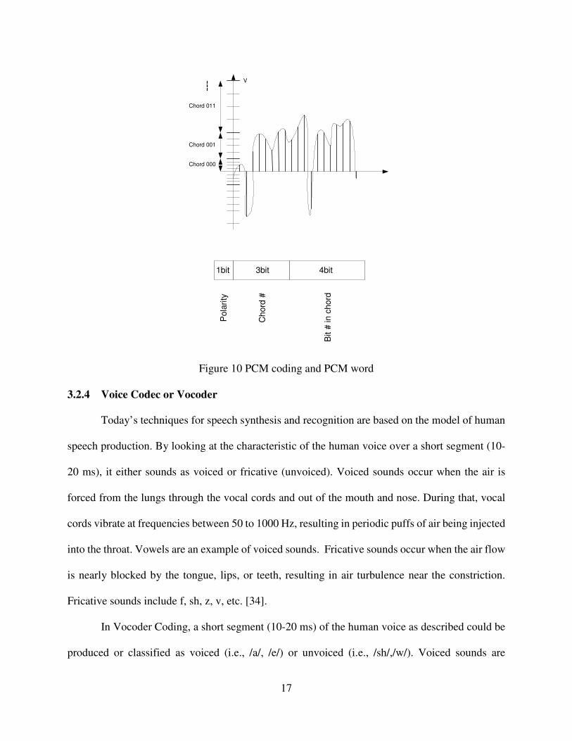
companding is depicted by equation (1). Per ITU G.711, each PCM word consists of three parts as
shown in Figure 10. The first bit is the polarity bit, the next three bits represent chord number, and
the remaining four bits represent one of 16 possible steps within a chord. Chords are spaced
logarithmically, whereas steps within the chord are linearly spaced.
� = � ��(����) ; 0 ≤ ������� (��)(���� ; �� ≤ � ≤ � (1)
where v represents the instantaneous input amplitude, A is a constant set to 87.56, and V represents
the maximum input amplitude.
The behavior of µ-law companding is represented by equation (2):
� = ��� (����)��� (���) (2)
where µ has a constant value of 255 and x has value of v/V and varies between -1 and 1.
Usually the A/D IC (Integrated Circuit) consists of a built-in PCM hardcode with A-law
and µ-law selection [34]. In practice, these three processing steps (sampling, quantization and
encoding) could take place simultaneously.
17
Chord 011
Chord 001
Chord 000
V
Pola
rity
Ch
ord
#
Bit #
in c
hord
1bit 3bit 4bit
Figure 10 PCM coding and PCM word
3.2.4 Voice Codec or Vocoder
Today’s techniques for speech synthesis and recognition are based on the model of human
speech production. By looking at the characteristic of the human voice over a short segment (10-
20 ms), it either sounds as voiced or fricative (unvoiced). Voiced sounds occur when the air is
forced from the lungs through the vocal cords and out of the mouth and nose. During that, vocal
cords vibrate at frequencies between 50 to 1000 Hz, resulting in periodic puffs of air being injected
into the throat. Vowels are an example of voiced sounds. Fricative sounds occur when the air flow
is nearly blocked by the tongue, lips, or teeth, resulting in air turbulence near the constriction.
Fricative sounds include f, sh, z, v, etc. [34].
In Vocoder Coding, a short segment (10-20 ms) of the human voice as described could be
produced or classified as voiced (i.e., /a/, /e/) or unvoiced (i.e., /sh/,/w/). Voiced sounds are
18
represented by the periodic excitation with the pitch (i.e., fundamental frequencies) being an
adjustable parameter. On the other hand, an unvoiced sound is more like a random noise generator.
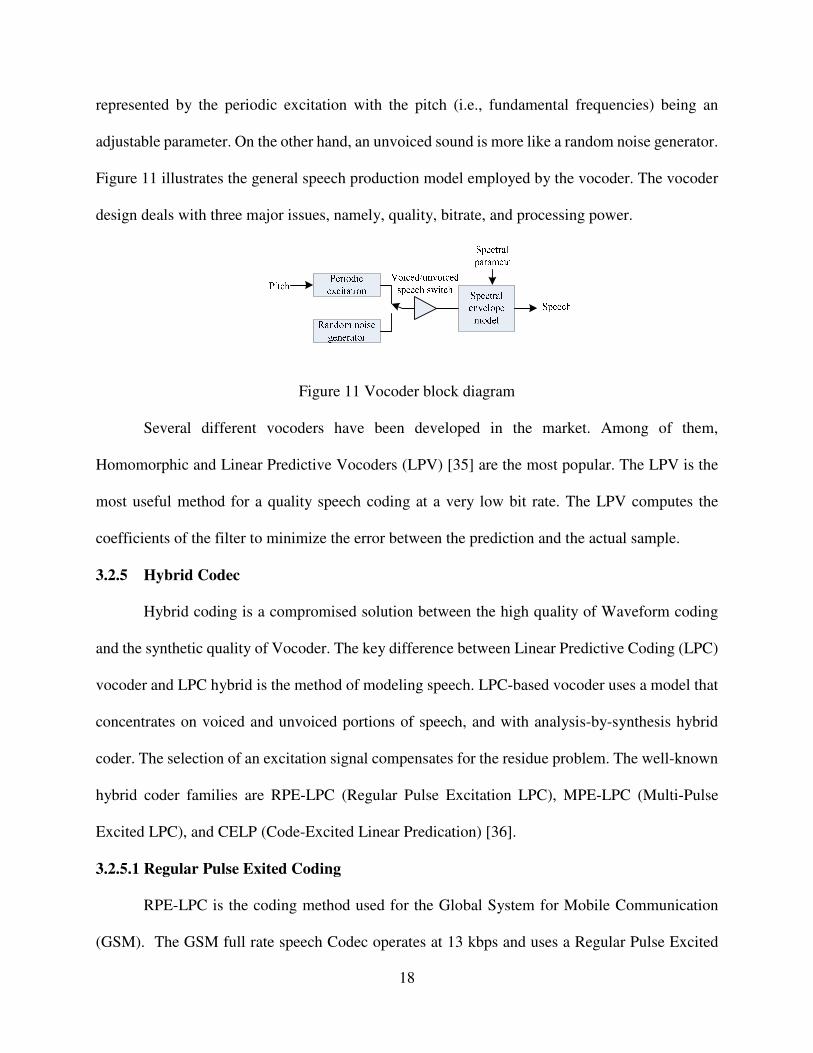
Figure 11 illustrates the general speech production model employed by the vocoder. The vocoder
design deals with three major issues, namely, quality, bitrate, and processing power.
Figure 11 Vocoder block diagram
Several different vocoders have been developed in the market. Among of them,
Homomorphic and Linear Predictive Vocoders (LPV) [35] are the most popular. The LPV is the
most useful method for a quality speech coding at a very low bit rate. The LPV computes the
coefficients of the filter to minimize the error between the prediction and the actual sample.
3.2.5 Hybrid Codec
Hybrid coding is a compromised solution between the high quality of Waveform coding
and the synthetic quality of Vocoder. The key difference between Linear Predictive Coding (LPC)
vocoder and LPC hybrid is the method of modeling speech. LPC-based vocoder uses a model that
concentrates on voiced and unvoiced portions of speech, and with analysis-by-synthesis hybrid
coder. The selection of an excitation signal compensates for the residue problem. The well-known
hybrid coder families are RPE-LPC (Regular Pulse Excitation LPC), MPE-LPC (Multi-Pulse
Excited LPC), and CELP (Code-Excited Linear Predication) [36].
3.2.5.1 Regular Pulse Exited Coding
RPE-LPC is the coding method used for the Global System for Mobile Communication
(GSM). The GSM full rate speech Codec operates at 13 kbps and uses a Regular Pulse Excited

19
(RPE) Codec [35]. In the RPE, the length of speech frame segment is 20 ms long, and each frame
contains a set of eight short-term predictor coefficients. Each frame is then further split into four
5 ms sub-frames, and for each sub-frame, a delay and gain for the Codec's long-term predictor will
be decided by the encoder. The residual signal after both short and long term filtering is quantized
for each sub-frame [37]. The residual signal of forty samples is decimated into three possible
excitation sequences, each consisting of 13 samples. The best representation of the excitation
sequence and each pulse in the sequence has its amplitude quantized with three bits which will be
chosen by the sequence with the highest energy.
At the decoder, the reconstructed excitation signal is fed through the long-term and the
short-term synthesis filters to give the reconstructed speech. A post filter is used to improve the
perceptual quality of this reconstructed speech. The GSM Codec provides good quality speech,
although not as good as slightly higher rate G728 Codec. However, the main advantage of GSM
Codec over other low rate Codecs is its relative simplicity.
The RPE-LPC GSM representative is GSM 06.10.
3.2.5.2 Multi Pulse Excited Coding
Figure 12 shows the block diagram of an LPC speech synthesizer with multi-pulse
excitation (MPE-LPC). Compared with the traditional LPC synthesizer, MPE-LPC doesn’t have
the pulse and white noise generators and the voiced-unvoiced switch. The excitation for the all-
pole filter is generated by an excitation generator that produces a sequence of pulses located at
times t1, t2 ,… tn… with amplitudes a1, a1, … an…, respectively. If desired, a pole-zero filter could
replace the all-pole filter. The sampled output of the all-pole filter is passed through a low-pass
filter to produce a continuous speech waveform ��.

20
In MPE-LPC, pulse position is found by an exhaustive search based on minimized mean
squared error as shown in Figure 13 [38].
tS
nS
Figure 12 LPC speech synthesizer with multi pulse excitation
netS
Figure 13 Analysis-by-synthesis procedure for the multi-pulse excitation
Due to its synthetic quality, MPE-LPC is no longer very popular.
3.2.5.3 Code Excited Linear Predictor (CELP) Coders
CELP [39] employs both waveform and vocoding techniques. In CELP, speech is passed
through a vocal tract and pitch predictor, an index from codebook will be used in place of an actual
quantization of the excitation signal (see Figures 14 and 15). The data rate of CELP is between 4.8
and 16 kbps. Some versions of CELP are listed below:
• FS 1016: Data rate is 4.8 kbps. It is the U.S Department of Defense standard.
• The G.728 Recommendation: An ITU standard, operates at 16 kbps, and provides
toll-quality speech comparable to the 32 kbps ADPCM.
• The G.729 Recommendation: An ITU standard, operates at 8 kbps. Due to the
complexity of G.729, several annexes are written for G.729.

21
)(kx)
)(ku
)(1
1
zP− )(1
1
zA− )/(1
)(1
yzA
zA
−
−
)(ke
)(kx
Figure 14 CELP encoder
Figure 15 CELP decoder
• The G.723.1 Recommendation: An ITU standard coder, operates at 5.3 and 6.3
kbps.
• Vector sum excited linear prediction (VSELP), a speech coding method used in
several cellular standards, including IS-54 and IS-136 (2G mobile phone system).
The VSELP algorithm is known as an analysis-by-synthesis coding technique. It
belongs to the class of CELP.
• Algebraic Code Excited Linear Prediction (ACELP) is patented by VoiceAge
Corporation. It has a limited set of pulses which is distributed as excitation to linear
prediction filter. The representatives of ACELP are GSM 06.20 Half-Rate (HR)
and GSM 06.60 Enhanced Full Rate (EFR).

22
3.2.6 Other Vocoders
Since different Codecs could be implemented on the same hardware platform; there are
several other free-of-charge Codecs which have been developed by the open source community as
the alternative for licensed Codecs, utilizing the power of the open source community.
3.2.6.1 Internet Low Bit-rate Codec (iLBC)
The iLBC is a VoIP Codec created by Global IP Sound. iLBC (internet Low Bit-rate
Codec) is a free speech Codec suitable for robust voice communication over IP [26]. iLBC is
designed for narrow band speech. It has a payload bit rate of 13.33 kbps with an encoding frame
length of 30 ms. It also has a bit rate of 15.20 kbps with an encoding length of 20 ms. This Codec
is equipped with graceful speech quality degradation in the case of lost frames, which occur in
connection with lost or delayed IP packets [39]. Global IP sound’s aim is for iLBC to have a basic
quality and robustness to packet loss higher than G.729A, and the computational complexity
similar to G.729A.
3.2.6.2 GIPS
Originally, GIPS [40] was also created by Global IP Sound. The owner claims to be able
to maintain voice quality even with 30% packet loss. GIPS is the technology licensed for use by
Skype. It is being made an IETF standard. GIPS operate at bit rates of 13.3 kbps and up. GIPS
wideband Codecs (16 kHz sample rate) include:
• iSAC: Internet Speech Audio Codec is a high-efficiency variable bit rate Codec.
iSAC is targeted for low data rate connections including dialup. It most closely
matches the one described as being used by the Skype client.
• iPCM-wb: Internet Pulse Code Modulation wide-band for higher rate connections.
23
3.2.6.3 Speex
Speex [26,40] is an Open Source/Free Software patent-free designed for speech. Per Speex
Project team, it is free of charge to lower the barrier of entry for voice applications. Speex is well-
adapted to Internet applications. It also provides useful features that are not present in most of the
other Codecs. Today, Speex is part of the GNU Project and is available under the Xiph.org variant
of the BSD license. Speex is a great Codec due to its flexibility. However, it is also an expensive
Codec since it consumes more CPU power than the G729, G726 or GSM Codecs, and just about
the same as iLBC.
3.2.6.4 LPC-10
The LPC-10 Codec derives its name because it uses 10 LP coefficients. The LPC-10
operates at a bit rate of 2.4 kbps and with a total of 54 bits per frame. LPC-10 is used for narrow
bandwidth connections. The disadvantages of using LPC-10 are [41] listed below:
• Decoded voice can sound very “buzzy” which is caused by parameter updates.
• Poor LP modeling results in wide bandwidths and rapid decay of the pulse
excitation.
• Regularly voiced excitation is unnatural - normally some jitter.
• Voicing errors produce significant distortions.
• Binary voicing decision is sometimes poor.
• Not suited to model nasals - although okay in practice.
• Only models speech – does not work if background noise exists (i.e., not suited to
mobile phone applications without further work).

24
3.2.7 Media Format Codecs
Media format high-quality Codecs, such as MP3 (MPEG audio layer III), AAC (Advanced
Audio Codec), WMA (Windows Media Audio), Ogg Vorbis, etc… are used in Audio storage, i.e.,
CD, Television, DVD, Blue-ray, camcorder, etc… Due to one or more of the following reasons
such as high complexity, high bit rate, and long delay, media format Codecs have not been used
for real-time VoIP conversation. However, they could be used for music on hold or recorded
announcements playback. Vorbis Codec is a free and open source Codec. Its quality is comparable
with other commercial Codecs (MP3, WMA, AAC…). Typical of media format Codec for music
Vorbis Codec have a bit rate of 128 kbps. Encoding and decoding delay times are not revealed, in
fact from seconds to minutes. Even if media Codecs are used for music on hold application, the
playback bit rate will be very low. We shall, therefore, concentrate on the Speech Codec, and will
not have further discussion on media format Codecs.
3.2.8 Codec Loss Concealment Algorithm
In order to reduce the impact of frame loss [42], some Codecs such as G.729, G.723.1,
AMR and the iLBC have a built-in loss concealment algorithm. The loss concealment algorithm
can interpolate the parameters for the loss frames from the parameters of previous frames. For
example, in the G.729 Codec, the loss concealment algorithm repeats the line spectral pair
coefficients of the last good frame. The adaptive and fixed codebook gain will be taken from the
previous frames. However, they are damped to reduce their impact gradually. The fixed codebook
contribution will be set to zero if the last reconstructed frame was classified as voiced, The pitch
delay is taken from the previous frame and is repeated for each of the following frames. The
adaptive codebook contribution will be set to zero, and the fixed codebook vector will be randomly
chosen if the last reconstructed frame was classified as unvoiced. In other words, if a frame is not

25
losing all parameters, it will be re-constructed based on received and previous parameters instead
of replacing the whole frame with interleaving frame, which is the previous reconstructed frame.
3.3 Evaluation of Speech Codecs
In general, the performance of speech and audio Codecs is evaluated using six attributes:
bit rate, speech quality, signal delay, complexity, robustness to acoustic noise, and robustness to
channel errors. The desired Codec must have low bit rate, low delay, less complexity, but high
speech quality. Speech quality can be determined both subjectively and objectively.
3.3.1 Subjective Measures
Subjective measurements are obtained from the listening tests, whereas objective
measurements are computed directly from the coded speech parameters. Some common subjective
measures are listed below:
• Diagnostic Rhyme Test (DRT): It uses a set of isolated words to test for consonant
intelligibility in initial position. The DRT is one of the ANSI S3.2-2009 standards
for measuring the intelligibility of speech over communication systems.
• Paired Comparison Test (PCT): Pair comparison method is usually used to test the
overall system acceptance. It is based on a speech synthesizer listener which will
listen to artificial speech for hours per day [43-44]. Stimuli from each synthesizer
will be compared in pairs with all n(n-1)/2 combinations. If there are more than one
test sentence (m), each version of a sentence will be compared to all the other
version. Thus there will be a total number of n(n-1)m/2 comparison pairs.
• Mean Opinion Score (MOS): The listener's task is simply to evaluate the tested
speech with scale described in Table 1. In Unified Communication (UC), there are
two classes of MOS, listening quality (MOS-LQ) and conversional quality (MOS-

26
CQ). Another MOS scale, is known as the DMOS (Degradation MOS) or the DCR
(Degradation Category Rating) and it is an impairment grading scale to measure
how the different disturbances in speech signal are perceived (Absolute Category
Rating).
Table 1 Scales used in MOS and DMOS
RATING MOS (ACR) DMOS (DCR)
5 Excellent Inaudible
4 Good Audible but not annoying
3 Fair Slightly annoying
2 Poor Annoying
1 Bad Very annoying
Calls made over the PSTN have a MOS score of around 4.3, while the vocoders used in
wireless telephone system, i.e., GSM (Global System for Mobile Communication), CDMA (Code
Division Multiple Access) and TDMS (Time-Division Multiplexing System) have MOS score
ranging from 3.4 to 3.9. The subjective measures give a wide variation among listener scores since
the scales used by the listeners are not calibrated and do not provide an absolute measure. In VoIP
application, subjective measures do not indicate specific network impairment, which is important
for VoIP quality control. The objective measures indicate multiple factors, including network
impairment status, and therefore has been widely used in VoIP control and monitoring.
3.3.2 Objective Measures
H. Özer et al. [5] categorize the objective measures into perceptual and non-perceptual
groups. The non-perceptual group is further divided into time-domain and frequency-domain
measures. The metrics used in time domain measure of speech quality includes Segmental Signal-
to-Noise Ratio (SNRseg), Signal-to-Noise Ratio (a special case of SNRseg), Czenakowski
Distance (CZD). The metrics used in frequency domain measure of speech quality includes Log-
Likelihood Ratio (LLR), Log Area Ratio (LAR), Itakura-Satio Distance measure (IS or ISD),

27
COSH Distance measure (COSH), Cepstral Distance Measure (CDM), Spectral Phase (SP),
Spectral Phase-Magnitude distortion (SPM), and Short Time Fourier-Radon Transform measure
(STFRT). The perceptual group of speech quality measure includes Barker Spectral Distortion
(BSD), Modified Barker Spectral Distortion (MBSD), Enhanced Modified Barker Spectral
Distortion (EMBSD), Perceptual Audio Quality Measure (PAQM), Perceptual Speech Quality
Measure (PSQM), Weighted Slope Spectral Distance Measure (WSSD), and Measuring
Normalizing Blocks (MNB). A select set of above-mentioned measures calculate distortion from
the overall data, namely, SNR, CZD, SP and SPM. On the other hand, the distortion is calculated
for small segments and then the average is taken over all the segments to obtain the overall speech
quality measure. The measures using the averaging include SNRseg, BSD, MBSD, EBSD, PAQM,
PSQM, LLR, LAR, ISD, COSH, CDM, and WSSD. The segment length is 20 ms (320 samples
for 16 kHz signal), which is used as window size for the techniques MNBs and STFRT.
Another way to classify objective measure is intrusive or non-intrusive. Intrusive or non-
intrusive measures relate to voice quality measurement over the network. Intrusive methods are
more accurate but are usually unsuitable for monitoring live traffic because of the need for
reference data and access to the network. Current non-intrusive methods rely on subjective tests to
derive model parameters. Therefore these methods are limited and do not meet new and emerging
applications.
3.3.2.1 Time-Domain Measures
Time-domain measures compare the two waveforms – the original audio signal, x(i) and
the recovered audio signal, y(i) in the time domain. Some popular time-domain measures are:
Segmental Signal-to-Noise Ratio (SNRseg) is defined in equation (3) as the average of the
SNR values over small segments:

28
����� = �!" ∑ log"'�()! (∑ ( �*(�)(�(�)'+(�))*,(�-'��),( ) (3)
The length of the segment is typically 15 to 20 ms for speech. The SNRseg is applied to
frames with energy above a specified threshold in order to avoid silence regions.
Signal-to-Noise Ratio (SNR) in equation (4) is a special case of SNRseg, when M=1 and
one segment encompasses the whole record. The SNR is very sensitive to the time alignment of
the original and the distorted audio signal. The SNR is measured as:
��� = 10 log ( ∑ �*(�)/012∑ (�(�)'+(�))*/012 ) (4)
This measure has been criticized for being a poor estimator of subjective audio quality.
Czenakowski Distance (CZD) is a correlation-based metric, which directly compares the
time-domain sample vectors as shown by equation (5):
3 = �, ∑ (1 − 5∗789 (�(�),+(�))�(�)�+(�) ),�'� (5)
3.3.2.2 Frequency-Domain Measures
Frequency-domain measures (e.g. LLR, LAR, ISD, COSH, CDM, WSSD, SPD, SPMD,
STFRT) [5] compare the original and recovered signals on the basis of their spectra or in terms of
a linear model based on second order statistics [45].
Log-Likelihood Ratio (LLR), also known as Itakura distance, considers an all-pole linear
predictive coding (LPC) model of the speech segment, ;(<) = ∑ =(>);(< − >) + @A()� B(<)
where, a(m) are the prediction coefficients, p is the filter order, and u(n) is an appropriate
excitation source. The LLR measure is then defined by equation (6):
CC� = log DE�FGHE�EHFGHEHI (6)
where =� is the LPC coefficient vector for the original signal x(n), =+ is the corresponding vector
for the recovered signal y(n), with respective covariance matrix �+.

29
Log Area Ratio (LAR) is another LPC-based technique, which uses partial correlation
(parcor) coefficients. The parcor coefficients form a parameter set derived from the short-time
LPC representation of the speech signal under test. The LAR will be delivered from area ratio
functions of these coefficients as equation (7):
CJ�� = log K ��0L2M = log K��N2�'N2M, JA�� = 1 (7)
where iα is the ith parcor coefficient, which can be found by using equation (8):
O = O�(�) , 1 ≤ P ≤ Q (8)
where O�(�) is the ith LPC calculated by using the ith order LPC model.
Itakura-Saito Distance Measure (ISD) is the discrepancy between the power spectrum of
the recovered signal Y(w) and that of the original audio signal X(w):
R� = �5S T KU(V)W(V) − log U(V)W(V) − 1M XYS'S (9)
COSH Distance Measure is the symmetric version of the ISD. Here the overall measure is
calculated by averaging the COSH values over the small segments:
3Z�[ = �5S T \�5 ]KU(V)W(V) + W(V)U(V)M − log KU(V)W(V) + W(V)U(V)M − 2_` XYS'S (10)
Cepstral Distance Measure (CDM) is a distance, defined between the cepstral coefficients
of the original and recovered signals. The cepstral coefficients can also be computed by using LPC
parameters. An audio quality measure for the mth frame based on the L cepstral coefficients, cx(k)
and cy(k), of the original and recovered signals respectively, is given by equation (11a):
Xab�, b+ , >c = Kdb� − b+(0)e5 + 2 ∑ db�(f) − b+(f)e5gh)� M�/5 (11a)

30
The overall distortion is calculated over all frames using equation (11b).
3j = ∑ V(()k(l�,lH,()mn12∑ V(()mn12 (11b)
where M is the total number of frames, and w(m) is a weight associated with the mth frame.
For example, the weighting could be the energy in the reference frame. It is typical to use
a 20 ms frame length and the energy of the frame as weights.
In Spectral Phase and Spectral Phase-Magnitude Distortions, the phase and/or magnitude
spectrum differences have been observed to be sensitive to image and data hiding artifacts. They
are defined by equations (12) and (13).
�o = �, K∑ pq�(Y) − q+(Y)p5,V)� M (12)
�or = �, Kλ ∑ pq�(Y) − q+(Y)p5 + (1 − t) ∑ ||v(Y) − |�(Y)||5,V)�,V)� M (13)
where SP is the spectral phase distortion, SPM is the spectral phase-magnitude distortion, q�(Y) is
the phase spectrum of the original signal, and q+(Y) is the phase spectrum of the distorted signal,
X(w) is the magnitude spectrum of the original signal, Y(w) is magnitude spectrum of the distorted
signal, and λ is chosen to attach commensurate weights to the phase and magnitude terms.
Short-Time Fourier-Radon Transform Measure (STFRT) is a multi-dimensional measure,
based on Short-Time Fourier Transform (STFT). Given a Short-Time Fourier transform (STFT)
of a signal, its time projection provides the magnitude spectrum while its frequency projection
yields the magnitude of the signal itself. By considering all the other dimensions rather than taking
only the vertical and horizontal projections, the Radon transform of the STFT measure could be
obtained. STFRT is the objective audio quality measure based on the mean-square distance of
Radon transforms of the STFT of two signals.
31
3.3.2.3 Perceptual Measures
Perceptual measures, such as WSSD, BSD, MBSD, EMBSD, PAQM, PSQM, and MNB,
take explicitly into account the properties of the human auditory system [5].
Bark Spectral Distortion (BSD) is assuming that speech quality is directly related to speech
loudness. The BSD estimates the overall distortion based on the average Euclidian distance
between loudness vectors of the original and the distorted audio. The Bark spectral distortion in
[45] is calculated using equation (14) as shown below:
w�j = ∑ d��(P) − �+(P)e5x�)� (14)
where K is the number of critical bands, ��(P) is the Bark spectra of the ith critical band
corresponding to the original, and �+(P) is the coded speech.
For speech, 18 critical bands (which is up to 3.7 kHz) are used. The overall distortion will
be calculated based on averaging the BSD values.
Modified Bark Spectral Distortion (MBSD) is a modification of the BSD. MBSD
incorporates noise-masking threshold to differentiate between audible and inaudible distortions.
The inaudible loudness difference, which is proportional to ��(P) − �+(P) and below the noise-
masking threshold will be excluded in the calculation of the perceptual distortion. The perceptual
distortion of the nth frame is the sum of the loudness difference which is greater than the noise
masking threshold as shown on following equation (15) as:
r�wj = ∑ r(P)j�+(P)x�)� (15)
where M(i) denote the indicator of perceptible distortion and j�+(P) is the loudness difference in
the ith critical band, and K is the number of critical bands.
The global MBSD value will be calculated by averaging the MBSD scores over non-silence
frames [5].

32
Enhanced Modified Bark Spectral Distortion (EMBSD) is a variation of MBSD. In
EMBSD, only the first 15 loudness components (instead of the 24-Bark bands) will be used to
calculate loudness differences. Loudness vector is normalized, and a new cognition model will be
assumed based on post-masking effects as well as temporal masking.
In Perceptual Audio Quality Measure (PAQM), a model for emulating the human auditory
system will be used. The transformation from the physical to the psychophysical domain is
performed by time-frequency spreading and level compression, for example masking behavior of
the human auditory system is taken into account. In the beginning, the reference and coded signals
are transformed into short-time Fourier domain (Figure 16), then the frequency scale will be
converted into pitch scale (in bark) and the signal will be filtered to transfer from outer ear to inner
ear. These results will be in the power-time-pitch representation. Therefore, the resulting signals
will have frequency domain smearing and time domain smearing. Per Thilo Thield and Ersnt Kabot
of Technical University of Berlin and others, the measure of the quality of an audio system is an
average of comparison.
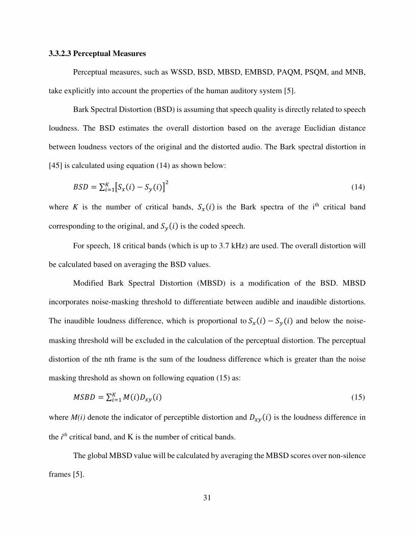
Perceptual Speech Quality Measure (PSQM) was devised by Beerends in 1993. This
development represents an adapted version of the more general perceptual audio quality measure
(PAQM), which is optimized for telephony speech signals. PSQM is a modified version of the
PAQM [45], in fact, the optimized version for speech. PSQM does not include temporal or spectral
masking for loudness computation. PSQM applies a nonlinear scaling factor to the loudness vector
of distorted speech. PSQM has been adopted as the ITU-T Recommendation P.861, its detailed
block diagram shown in Figure 17 which illustrates how to calculate PSQM. The P.861is end-of-
life, its successor, is P.682 – Perceptual Evaluation of Speech Quality (PESQ). Our research has
no intention to develop any test using PSQM.

33
The Perceptual Evaluation of Speech Quality (PESQ) model begins by a standard listening
level aligning both signals, then modeling a standard handset by filtering (using an FFT) with an
input filter. The signals are then processed through an auditory transform which is similar to that
of PSQM. At this process, there is also an equalizing for linear filtering and for gain variation.
Two distortion parameters will be extracted from the disturbance, and will be aggregated into
frequency and time, and will be mapped to a prediction of subjective MOS.
The PESQ aims to have more suitability with the nowadays network, especially VoIP, in
comparison with previous models, i.e., PSQM, BSD, etc., PESQ has better performance to deal
with prediction accuracy, taking proper account of noise or packet loss, delay jitter, etc.
Weighted Slope Spectral Distance Measure (WSSD) uses a filter bank [46], consisting of
thirty-six overlapping filters of progressively larger bandwidth which can make short-time audio
spectrum smoother. The filter bandwidths approximate critical bands in order to give equal
perceptual weight to each band. Klatt [47-48] uses weighted differences between the spectral
slopes in each band because the spectral variation could play a major role in human perception of
audio quality. The spectral slope is computed in each critical band as:
��(f) = v(f + 1) − v(f) (16a)
�+(f) = �(f + 1) − �(f) (16b)
where k is the critical band index, X(k) and Y(k) are the spectra in decibels, and )}(),({ kVkV yx are
the first order slopes of these spectra.
Next, a weight for each band is calculated based on the magnitude of the spectrum in that
band as shown in equation (17).
y��j = ∑ Y(f)[��(f) − �+(f)]5|}h)� (17)
where, the weight w(m) is chosen according to a spectral maximum.

34
WSSD is computed separately for each 12 ms audio segment and then by averaging the
overall distance.
Measuring Normalizing Blocks (MNB) is an objective speech measure that provides an
algorithmic estimate for rating human subjects that will give coded or degraded speech [49]. It is
based on a model of human auditory perception and has been optimized against a large number of
human-rated speech passages. In MNB the important role of the cognition module for estimating
speech quality has been emphasized. MNB is sensitive to the relative delay between the reference
and the test signals. The human listeners’ sensitivity to the distribution of distortion is considered
in MNB, so MNB uses hierarchical structures that have a time and frequency scales from larger to
smaller. MNB integrates over frequency scales. It measures differences over time intervals. It also
integrates over time intervals, and it measures differences over frequency scales. These MNBs is
then linearly combined to estimate overall speech distortion.
Figure 16 Perceptual Audio Quality Measure (PAQM)
35
Figure 17 PSQM calculation procedure
3.4 Objective Quality Measures Evaluation
In this research, we have performed all of the tests for the object quality measures
mentioned in section 3.3.2 and compared with the listening evaluation. We found that all objective
measures performances are not linear with MOS. Each objective measure result depends on the
language and background noise. All measures were performed with off-line samples with no
network impact. The final voice quality of a VoIP channel, in fact, depends on many other factors,

36
included but not limited to network quality. The voice quality of a VoIP channel will be discussed
in following sections. In conclusion, PESQ is selected as the preferred method for speech Codec
evaluation, due to its accuracy and its simplicity.
3.5 Selection of Speech Codecs
While legacy public switched telephone network (PSTN) has a dedicated medium for voice
transmission, VoIP uses Internet service medium for transmission. In addition, VoIP stream is
always carried out using packetized form (packet voice) which has an IP header. As a result, VoIP
has a higher delay and higher packet loss probability. The selection of Codec for VoIP depends on
the network quality and Codec specification. The lower bit-rate Codec is preferred for low
bandwidth service; the small packet is preferred for long delay network. Selecting a Codec is also
based on Processor power versus Codec complexity.
Variable Bit Rate (VBR) Codec has been developed, however, the bit rate change was
based on the speech property itself. The Codec selection or bit rate could be changed based on
network condition or by class of service that is paid by the client. Emmanuel Antwi-Boasiako et
al. [26] has performed a test on two popular Codecs, G.711 and Speex with objective Perceptual
Evaluation of Speech Quality (PESQ) and subjective Mean Opinion Score (MOS). The report did
not mention whether a narrow band or wide band Speex has been used for testing. There is other
research on voice quality and bandwidth tradeoff and voice Codec for a specific language.
Among the number of Codecs for VoIP, the following are our rating for the Codecs from
the highest to the lowest:
• Speex for its flexibility, quality and low implementation cost, no license fee.
Especially with 16 kbps Speex quality is better than G.711’s.
• G.729 for its low bandwidth and good quality.

37
• G.711, Annex 1, higher bandwidth, good quality and good packet loss recovery, no
license fee.
• G.723 for the lowest bandwidth.
• iLBC, for open source VoIP application.
3.5.1 Codec Impairment
In ITU G.107 recommendation for VoIP transmission planning, E-model is used to
calculate the transmission rating factor R.
E-model is looking at both IP and non-IP factors which impact on VoIP QoS. Codec
impairment is represented as Ie-eff in the E-Model, which is described in ITU G.113 (Table I.1/ITU
G.113). More details of E-model by ITU and also mentioned by E. Myakotnykh [50] in his
dissertation will be presented in Chapter 4.
3.5.2 Codec vs. Bandwidth
Using Codec with low Ie-eff [51] is desirable. However, the Codec may not be selected
based on provisioning Ie-eff value only. Low compression and long interval Codec can cause higher
bandwidth, more delay, congestion, or packet loss. Codec selection is based on available
bandwidth. Using a Variable Bit Rate (VBR) Codec could improve the quality, however for
bandwidth planning a fixed bit rate will be used for calculation.
Most of the service providers will assist their customer based on bandwidth requirements.
From an academic standpoint, a simple calculation of the required bandwidth for a VoIP channel
has been proposed.
Assuming that minimum bandwidth B is requested to assure that there is no packet loss
caused by queuing delay, R is maximum Codec rate (bps), n is the number of packets per second
n= 1/Ts, where Ts is minimum Codec frame length.

38
Assuming that H is the header size (usually 40 bytes = 320 bits), Then minimum bandwidth
for VoIP is:
B = nH+R = R+H/Ts (18)
Below are two examples for G.729A and G.711:
(a) With G.729A, R=8 kbps, Ts=0.02 s, B = 8000+320/0.01 = 24 kbps.
(b) With G.711, R=64 kbps, Ts=0.02 s, B = 76 kbps.
Note that since the Variable Bit Rate (VBR) could be used, we use maximum Codec bit
rate and minimum frame length which haven't been mention by B. Goode [1] or B.
Ngamwongwattana [7] or others before. The frame length Ts typical is 20 ms and always less than
preferred maximum delay of 400 ms. Additional bandwidth may be required for signaling (out-
band signal). For reference, Table 2 provides the bandwidth requirement by Cisco [52].
Table 2 Provisional planning values for the equipment impairment factor Ie per ITU G.113
Codec Information Bandwidth Calculations
Codec & Bit Rate (Kbps)
Codec Sample
Size (Bytes)
Codec Sample Interval
(ms)
MOS
Voice Payload
Size (Bytes)
Voice Payload
Size (ms)
Packets Per
Second (PPS)
Bandwidth MP or
FRF.12 (Kbps)
Bandwidth w/cRTP MP or
FRF.12 (Kbps)
Bandwidth Ethernet (Kbps)
G.711 80 10 4.1 160 20 50 82.8 Kbps 67.6 Kbps 87.2 Kbps
(64 Kbps)
G.729 10 10 3.92 20 20 50 26.8 Kbps 11.6 Kbps 31.2 Kbps
(8 Kbps)
G.723.1 (6.3 Kbps)
24 30 3.9 24 30 34 18.9 Kbps 8.8 Kbps 21.9 Kbps
G.723.1 (5.3 Kbps)
20 30 3.8 20 30 34 17.9 Kbps 7.7 Kbps 20.8 Kbps
G.726 20 5 3.85 80 20 50 50.8 Kbps 35.6 Kbps 55.2 Kbps
(32 Kbps)
G.726 15 5 - 60 20 50 42.8 Kbps 27.6 Kbps 47.2 Kbps
(24 Kbps)
G.728 (16 Kbps)
10 5 3.61 60 30 34 28.5 Kbps 18.4 Kbps 31.5 Kbps

39
3.5.3 Codec vs. Complexity
Even though Codec processor power (Million instructions per second - MIPS) is not a
concern for engineers nowadays, typical encoding and decoding will be carried out by terminal
devices (phone) without any problem (DSP is capable of hundreds of MIPS). However, in channel
encoding and decoding, wherever traffic load is high, the cost for high MIPS implementation is an
issue. Variable Bit Rate (VBR) is desired to improve VoIP QoS, VBR Codec is more complicated
than CBR (Constant Bit Rate) Codec. However, nowadays the cost of very powerful DSP is
negligible, and therefore the complexity is no longer an issue.
3.5.4 Codec Selection Based on Implementation Cost
Choosing a Codec sometimes depends on the license fee. Most of VoIP servers using open
source are also using open source or license free Codecs such as G.711, GSM or Speex.
3.6 Speech Codec Summary and Future Challenges
VoIP is a real-time packet communication. Packet loss and delay jitter are two major
concerns when selecting a Codec. Language oriented Codec could be an approach for VoIP
Codecs. Applying noise and echo cancellation before compressing the speech is always
recommended [53]. In addition, a Codec with other features, such as accent, language recognition,
could reduce the bit rate without reducing quality.
Speech Codec is used for packetizing in VoIP. Codec could use different compressing
techniques to reduce the bandwidth. Speech Codecs are specified as Waveform Codec, Vocoders,
and Hybrid coders. Codec quality evaluation could be objective or subjective. With the subjective
method, it could be intrusive or non-intrusive models. Codec has a dominant impact on the VoIP
quality. Selecting a Codec for VoIP is based on planning, including the provision of Codec
impairment, allocating bandwidth and service class. Using more complex Codecs or a Codec

40
translator can generate a significant delay. Future challenges of speech Codec work include
achieving lower bit-rate but higher quality, improvement in loss concealment and reduced
complexity.
41
CHAPTER 4: QUALITY CONTROL AND IMPROVEMENT
4.1 Overview
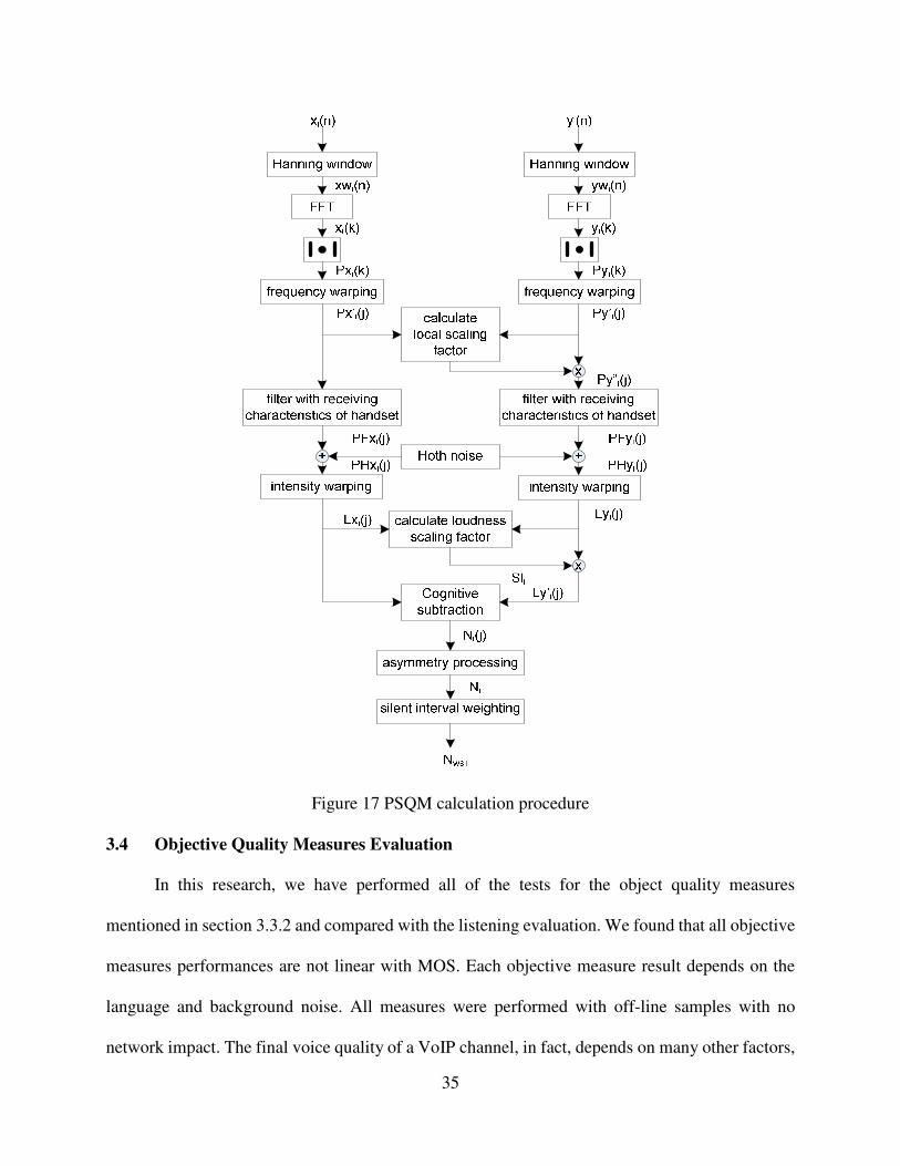
The VoIP perceived Quality of Service (QoS) is dependent on equipment impairment and
network quality as described in Figure 18. All Codec measures described in previous chapters are
used to measure the quality of speech Codec, which indicates the Codec impairment level only.
Voice over network quality depends on many factors including Codec quality and network quality.
It is necessary to have an objective measurement or prediction model, which includes all factors
that influence voice over network quality [54].
Figure 18 Perceived QoS zone
VoIP quality measurement includes subjective and objective methods. MOS is the well-
known subjective method while E-model is the most popular objective method.
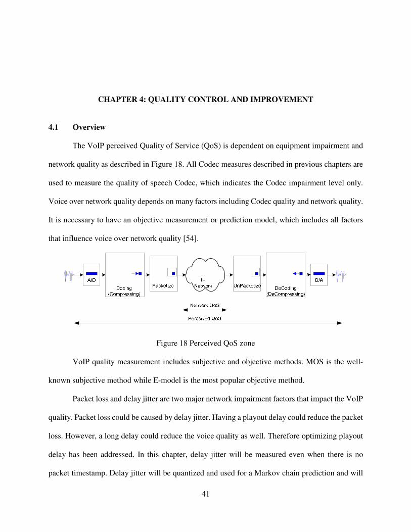
Packet loss and delay jitter are two major network impairment factors that impact the VoIP
quality. Packet loss could be caused by delay jitter. Having a playout delay could reduce the packet
loss. However, a long delay could reduce the voice quality as well. Therefore optimizing playout
delay has been addressed. In this chapter, delay jitter will be measured even when there is no
packet timestamp. Delay jitter will be quantized and used for a Markov chain prediction and will

42
be used to control playout delay time. Some of the experiment results will be provided to validate
this model. Other possible filters for jitter prediction such as Kalman filter [14] and packet loss
modeling that have been recently addressed will also be discussed.
4.2 Subjective Measurement
As mentioned in the previous chapter, Mean Opinion of Score (MOS), the subjective
measure used in voice communication is the most widely used and simplest method to evaluate
speech quality in general. The subjective measures give a wide variation among listener scores
since the scales used by the listeners are not calibrated and do not provide an absolute measure
[55]. In VoIP application [7], subjective measures do not indicate specific network impairment,
which is necessary for VoIP quality control. The objective measures indicate multiple factors [56],
including network impairment status, and this is the reason why it is widely used in VoIP control
and monitoring.
4.3 Objective Measurement
VoIP quality is dependent on the IP network and the end-point process quality. However,
subjective measures do not indicate specific network impairment, which is important for VoIP
quality control. Our goal is to provide a VoIP QoS strategy that allows monitoring and planning
the QoS through the network from end to end, which includes:
• QoS of voice stream through the gateway.
• QoS of voice stream over local area network (LAN).
• QoS of voice stream over wide area network (WAN).
The strategy is to use objective measures that indicate multiple factors, including network
impairment status, which has been used widely in VoIP control and monitoring. The weight of
each impairment factors will reflect on the quality factor R of E-Model that will be discussed

43
below. R-factor will not only help the VoIP provider make the best trade-off decision between
latency (delay), jitter, echo, network congestion, packet loss, and arrival of packets in out-of-
sequence but also will be able to advice the VoIP users as to what they should do to control and
monitor the VoIP QoS at their end.
The R-factor was described in the ITU-T G.107 recommendation in the second half of
2004. It defines a computing model known as an E-model [50,57-58]. The R-factor is a well-tried
tool for transmission planning and for determining the combined impact of various transmission
parameters that influence the call quality. As shown in equation (19), all appropriate transmission
parameters are put together to calculate the R-factor as follows:
R = RO - IS - ID - IE-EFF + A (19)
where, RO is the basic signal-to-noise ratio, IS is impairment that occur simultaneously with speech
(e.g. quantization noise, received speech and sidetone levels), ID is impairment that is delayed with
respect to speech (e.g. talker/listener echo and absolute delay).
IE-EFF captures effects of special equipment or equipment impairment (e.g. Codecs, packet
loss and jitter), and A is an advantage factor (permitted range is from 0 to 20; 0 for wired line and
10 for GSM). A short form of (19) is:
R = R0’ - ID - IE-EFF (20)
where R0’ is representing non-network impairment factors, which usually comes as a default value.
It is well known that the R depends on loss and delay jitter; these impairments will be
represented by ID and IE-EFF.
The E-model is a non-intrusive voice quality prediction, however, it has a number of
limitations. For example, it is based on a complex set of fixed, empirical formulas and is limited
by the number of Codecs and network conditions (because subjective tests are required to derive

44
model parameters), which hinders its use in new and emerging applications. It is a static model
which cannot adapt to the dynamic environment of IP networks [59] and based on the assumption
that the individual impairment factors defined on the transmission rating scale are independent of
each other, which may not be true. R model, however, is useful for estimating the QoS of a VoIP
channel given static information, or a good measure for VoIP planning.
Table 3 Equipment impairment factor to bandwidth requirement for Codec (Source: Cisco)
Codec type Reference Operating rate kbit/s Ie-value
PCM (see Note) G.711 64 0 ADPCM G.726, G.727 40 2
G.721(1988), G.726, G.727 32 7
G.726, G.727 24 25 G.726, G.727 16 50 LD-CELP G.728 16 7 12.8 20 CS-ACELP G.729 8 10 G.729-A + VAD 8 11 VSELP IS-54 8 20 ACELP IS-641 7.4 10 QCELP IS-96a 8 21 RCELP IS-127 8 6
VSELP Japanese PDC 6.7 24
RPE-LTP GSM 06.10, Full-rate 13 20
VSELP GSM 06.20, Half-rate 5.6 23 ACELP GSM 06.60,Enhanced Full Rate 12.2 5 ACELP G.723.1 5.3 19
ITU has made an online tool available for E-model computing at: http://www.itu.int/ITU-
T/studygroups/com12/emodelv1/calcul.php (Figure 19) [60]. More information regarding to the
E-Model can be found at ITU website http://www.itu.int.
For MOS friendly user, equation (21) could be used to convert R-factor to MOS [29,50]:
rZ� = � 1 � < 0610*7*)100)(60(035.01 −
−−++ RRRR 0 < � < 1004.5 � > 0 (21)

45
4.4 Latency, Delay Jitter, and Packet Loss
On the network side, the VoIP quality is dependent on these major factors: Latency, delay
jitter and packet loss.
4.4.1 Latency
The delay time from “mouth to ear” of a VoIP channel include the following items:
• Transmission Delay: This delay depends on the speed or the data rate of the
communication link and the packet length. It is the amount of time required to
transmit all the packet's bits from the first bit to the last bit into the communication
link, and this delay is proportional to the packet length.
• Propagation Delay: This delay depends on the physical characteristics of the
communication link. Propagation delay is the time to transmit one bit over a link
(i.e., the delay between the transmissions of the packet last bit from the source to
the reception of last bit of the packet at the destination).
• Switching Delay: This is the time required to shift data packets through the various
network hardware components such as hubs, routers. This delay is a reflection of
the speed of the switching device, like transmission delay in a packet switch.
• Queuing Delay: This delay depends on the traffic on the communication link and
capacity of switching device. Queuing delay is the delay between the entry point of
a packet in the transmit queue to the actual transmission point of the message.
• Processing Delay: This delay depends on the speed of processor(s), load and type
of processing scheme. This is the delay to process, compress and de-compress
(Codec) data, and also other process such as echo cancellation.

46
Figure 19 An E-model calculation tool
Figure 20 illustrates total “mouth to ear” delay of a VoIP channel. The network delay is
not a constant for each packet as the queuing times are not the same. Delay and loss are two major
quality factors of a VoIP channel. Figure 21 illustrates the perceived voice quality based on
network and application performances and channel noise, whereas each factor could result in both
network and application performances.
• Network Performance:
o Switching delay: Queuing and switching delay.
o Propagation delay: The physical delay caused by physical propagation.
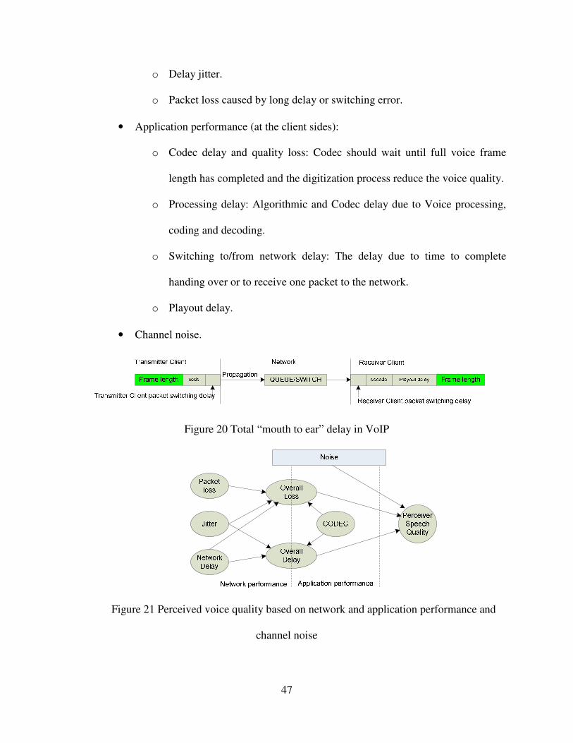
47
o Delay jitter.
o Packet loss caused by long delay or switching error.
• Application performance (at the client sides):
o Codec delay and quality loss: Codec should wait until full voice frame
length has completed and the digitization process reduce the voice quality.
o Processing delay: Algorithmic and Codec delay due to Voice processing,
coding and decoding.
o Switching to/from network delay: The delay due to time to complete
handing over or to receive one packet to the network.
o Playout delay.
• Channel noise.
Figure 20 Total “mouth to ear” delay in VoIP
Figure 21 Perceived voice quality based on network and application performance and
channel noise
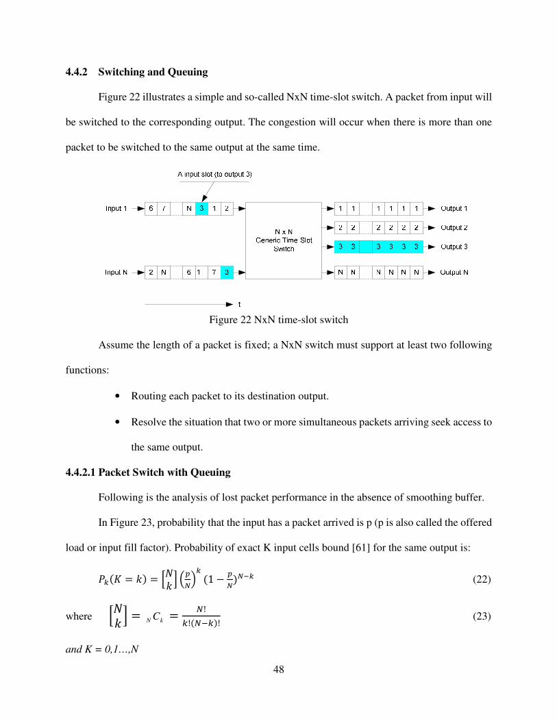
48
4.4.2 Switching and Queuing
Figure 22 illustrates a simple and so-called NxN time-slot switch. A packet from input will
be switched to the corresponding output. The congestion will occur when there is more than one
packet to be switched to the same output at the same time.
Figure 22 NxN time-slot switch
Assume the length of a packet is fixed; a NxN switch must support at least two following
functions:
• Routing each packet to its destination output.
• Resolve the situation that two or more simultaneous packets arriving seek access to
the same output.
4.4.2.1 Packet Switch with Queuing
Following is the analysis of lost packet performance in the absence of smoothing buffer.
In Figure 23, probability that the input has a packet arrived is p (p is also called the offered
load or input fill factor). Probability of exact K input cells bound [61] for the same output is:
oh(� = f) = \�f ` KA,Mh (1 − A,),'h (22)
where \�f ` = kN C = ,!h!(,'h)! (23)
and K = 0,1…,N

49
Average number of loss packet L for a given output per a time slot is
C = Q + K1 − A,M, − 1 and we obtain:
lim,→� C = Q − 1 + �'A
Thus, output fill factor F could be found as:
C = Q − C = 1 − K1 − A,M, and we obtain:
lim,→� � = Q − �'A (24)
The fraction of incoming cells that is lost by the switch FL is
�g = gA = 1 − �A + �A (1 − A,), (25)
With larger switch, the loss is more significant.
4.4.2.2 Input Queuing and Traffic-handling Capability of an Input-Queued Packet Switch
Figure 23 is an input queuing switch block diagram. Input FIFO (First In- First Out) buffer
is used to reduce the packet loss. The delay could be held up to (N)xT where T is the time slot
length. To reduce the delay time caused by waiting for “up-front” cell (so-called blocking), a
queued smoothing switch is utilized as shown in Figure 24. Each input has m buffers. Therefore
the time slot switch now is not NxN but NmxNm
Figure 23 Input queueing switch

50
Figure 24 Input smoothing queued switch
The probability of a output to be filled PF is:
o� = ∑ \�f ` K�,Mh,h'� K1 − �,M,'h = 1 − K1 − �,M, (26)
lim,→� o� = 1 − 1� = 63%
For large N, only about 63% of the output time slots are filled. That is the maximum load
for a packet switch [62].
4.4.2.3 Output Queuing
At the other end of the switch, the output could be in saturation, whereby the output would
have to wait until the link is available. Unlike input queuing which only need N queues, an output
queuing needs N2 queues.
Mean Delay for a Packet Switch with Output Queuing is described as following:
j = � �1 + A(�' 2/)5(�'A)� (27)
where T is time slot length.
When N = 1 the delay time is equal to a time slot length.

51
4.4.3 Packet Loss
For whatever reason, if voice frame is not ready to play after playout delay time is ended,
the packet that carries this frame is considered as lost. Packet latency exceeding the maximum
delay threshold or packet that has been routed to the wrong destination are the most common
packet loss situations.
4.5 Delay Jitter Measurement
4.5.1 Overview
Transmission delay jitter is the variance of transmitter delay [63]. Delay jitter causes the
packets not to arrive after the same durations as they were sent. Packet delay and delay jitter at the
receiver end (far-end) is used for quality monitoring and improvement. A practical method that
allows measuring of the approximately delay jitter from far-end of a streaming packetized
communication channel without packet timestamp has been introduced.
4.5.2 Delay Jitter in Packetized Communication
Assuming a streaming packetized communication channel, from packet start at the
transmitter side to packet arrival at the receiver side and ready to playout, has a total transmission
delay which could be simply expressed as:
D= Dconst + l + Dvar (28)
where
• Dconst is a minimum delay caused by any of sampling, coding, packetizing, queuing,
propagation, and not subject to change from one packet to another [34].
• l is the packet interval (frame length).

52
• Dvar is delay variance or Delay Jitter or Excess Delay or Jitter that could be different
for each packet, depending on traffic congestion, switching route, etc. and subject
to change from one packet to another.
Playout delay had been used to reduce the impact of jitter. Delay jitter is the base of playout
delay buffer.
4.5.3 Delay Jitter Measurement for Packet without Timestamp
There will be no issues with finding transmission delay if every packet has a timestamp at
both transmitter and receiver sides. However, this is not practical for packetized voice. Although
an IP transmission delay could be estimated with a synchronized packet which has timestamp
[7,8,64-65], voice packet may not have a timestamp on it. We have tried to assess the jitter without
knowing what time packet was sent and with or without synchronizing packet timestamp. Other
information we need is the packet number and frame length of each packet which is typically
included in the voice packet.
Let us assume a set of n+1 voice packets has arrived. This set gives us a set t consisting of
each packet arriving times and a set L consisting of each packet frame lengths:
t= {ti } , i = 1,..,n+1
L= {li} , i = 1,..,n+1
Ideally, packet number i will arrive after a duration of li-1.
From (28) we have the first packet arriving time is:
t1=t0 +Dconst + l1+J1
where t0 is the time first voice packet start and J1 is packet 1 delay jitter.

53
Packet 2 arriving time is:
t2 = t0 +Dconst +l1+ l2+J2
where t0 is the time first voice packet start and J2 is packet 2 delay jitter.
In general, we have:
�� = �! + jl-�� + ∑ �h �h)� + �� (29)
110 JDlt const +++
iconst
i
kk JDlt +++ ∑
=10
Figure 25 Packet voice arriving time
Removing frame lengths offset we obtain a substitute arrival time t’:
�′� = �� − ∑ �h �h)� = �! + jl-�� + �� (30)
Without loss of generality, we assume the minimum jitter is zero, or smallest value of t’
will be as follow:
Minimum (ti’) = m= t0 +Dconst+0
Thus we find the jitter set J by removing the offset m from (30).
�� = �′� − > (31)
Following are some special situations that could happen and the solution for each situation.
The loss of packet could lead to missing of one of the frame length value delays, and
equations (29), (30) and (31) will not have a solution. Since jitter J is not a negative value, we
suggest using minimum frame length for the lost packets.

54
In many applications, the Codec uses a preset constant frame length. Total frame lengths
offset in equations (29) and (20) could be written as:
∑ �h �h)� = P . � (32)
where l is the Codec frame length.
Most common application of using Jitter value is to decide the length of playout buffer.
Depending on the application scheme, the Jitter could be quantized to reduce the computation
complexity. In VoIP application, the quantized interval could be a minimum frame length.
We have used this method for a VoIP client application. The quantized jitter was used in
a Markov model for playout delay buffer sizing.
4.6 Playout Delay and Markov Model
In the packet voice application, playout delay (POD) is used to reduce the number of
packets loss caused by delay jitter. Longer POD will reduce the delay jitter loss; however, it will
also degrade the quality [7, 66]. Thus, an adaptive delay model is used to optimize the playout
delay. A practical adaptive POD based on Markov model has been introduced.
4.6.1 Delay Jitter in VoIP
In VoIP, if the frame length l is a constant, the total end to end delay (28) can be simply
expressed as:
D= Dconst +Dvar (33)
where Dconst is a minimum delay caused by sampling interval (frame length), coding, packetizing,
queuing, propagation, un-packetizing, decoding, assuming this will be the same for all packets.
Dvar is delay variable or Delay Jitter or Excess Delay or Jitter that could be difference for
each packet, depend on traffic congestion, switching route, etc.

55
The change of Dvar could cause the packets not to arrive in the same arrangement as when
they were sent out.
An example of no playout delay is shown in Figure 26, where the playout rule is simple as
first in – first out (FIFO) and no delay. Assume that the frame length is T, any received packet will
be played out immediately and the buffer size is infinity. The third packet and the fifth had some
delay jitters which cause an extra delay of arrival. Although the third packet jitter is smaller than
T, a part of the third packet could not be played without a gap between the second and the third
packet and an overlap at the beginning of the fourth packet. If the fifth packet jitter is greater than
a frame length T, it will not be played out and will be considered as a loss.
Figure 26 Packet loss when no delay plays-out or jitter buffer
Figure 27 illustrates how all packets will play out as they were sent for this example of
packet arrival and with the play out delay greater than the maximum Dvar.
In order for all arriving packets to play out in the right order, the delay should be greater
than the maximum Dvar. However, a longer delay will reduce the voice quality. An adaptive jitter
buffer will optimize the delay, thus, optimizing the QoS. The jitter buffer size is adjusted during
non-talk spurt periods.
Figure 27 Play out with a delay or jitter buffer greater than maximum delay jitter
4.6.2 Basics of Fixed and Adaptive Jitter Buffer Models
The common schemes of playout delay in VoIP are to set up a jitter buffer length based on
packet delay history. Typical fixed jitter buffer technique uses a statistical model, and adaptive

56
jitter buffer technique uses self-learning model. A fixed jitter buffer could use an average delay
jitter or a delay that is set by a packet loss threshold.
The adaptive model use the jitter history (statically) to predict upcoming jitter and adjust
buffer size accordingly. Markov [67-68] model for jitter prediction has been proposed. However,
the jitter will need to be rounded up to an integer number in order to be used as the Markov’s
states. In addition, jitter will be quantized to simplify the computation of Markov model [4].
From the results of our test, the smallest voice frame length T is recommended as the
quantized interval for Markov model, since delaying one voice frame could not impact too much
on the voice quality. The typical delay buffer dealing with the large jitter range could be over 200
ms. For example, for a voice packet length of 20 ms and maximum jitter of less than 400 ms will
have N = 20 states, or the transition matrix would be 20x20 only. If we use traditional jitter
measurement with 1 ms quantization, then the number of states would be 400, and the transition
matrix would be 400x400 instead.
A jitter delay tn will be quantized with interval T equal smallest Codec frame length and
its state i is:
P = R��(����� ) (34)
where function INT is identified as following:
P − 1 ≤ ����� < P , P = �1,2, … , <� (35)
where � is minimum of Codec frame length.
We can now obtain a set of states (sample space), S = {1,2,3…n).
Let us call:
N = max (Jk), k = 1,2,..,n. (36)
The Jk set will be used in the rest of the calculation.

57
4.7 Fixed Jitter Buffer Application
The packet which has jitter greater than playout delay will be considered as a lost packet.
If the playout delay is set as N, there will be no packet loss by jitter. However, the maximum delay
jitter could be very large. The voice quality will not be degraded significantly because of just one
or two packet loss. If the threshold for packet loss is identified as m (%) then we could find the
jitter buffer length L that satisfies that total percentage of delay jitter that greater than L is lesser
than m:
∑ ∑ Q�h,�)� ≤ >,h)g (37)
or
-�( ¡¢ £ ��E�¡� �¢E�¡¢ �¤E- g- ≤ > (38)
Eventually 1 < L ≤ N
The playout delay buffer therefore will be L instead of N.
Typically, we choose m = 1%.
4.8 Self-learning, Adaptive Markov Model Application
The Markov model has been studied recently [10, 69, 70]. However, no report has been
made on whether it has been tested or not. The research task is to investigate whether the method
is realistic and how good it is. The research task is also to find its practical application.
We can establish a transition probability matrix, which shows the likelihood of the move
from one state to another in the next step based on Markov. Figure 28 illustrates the probability of
transition from state i to state j up to three steps.
o = 1⋮�
1 … �¦Q�� Q�.. Q�,Q..� ⋱ Q..,Q,� Q,.. Q,,¨ (39)
where
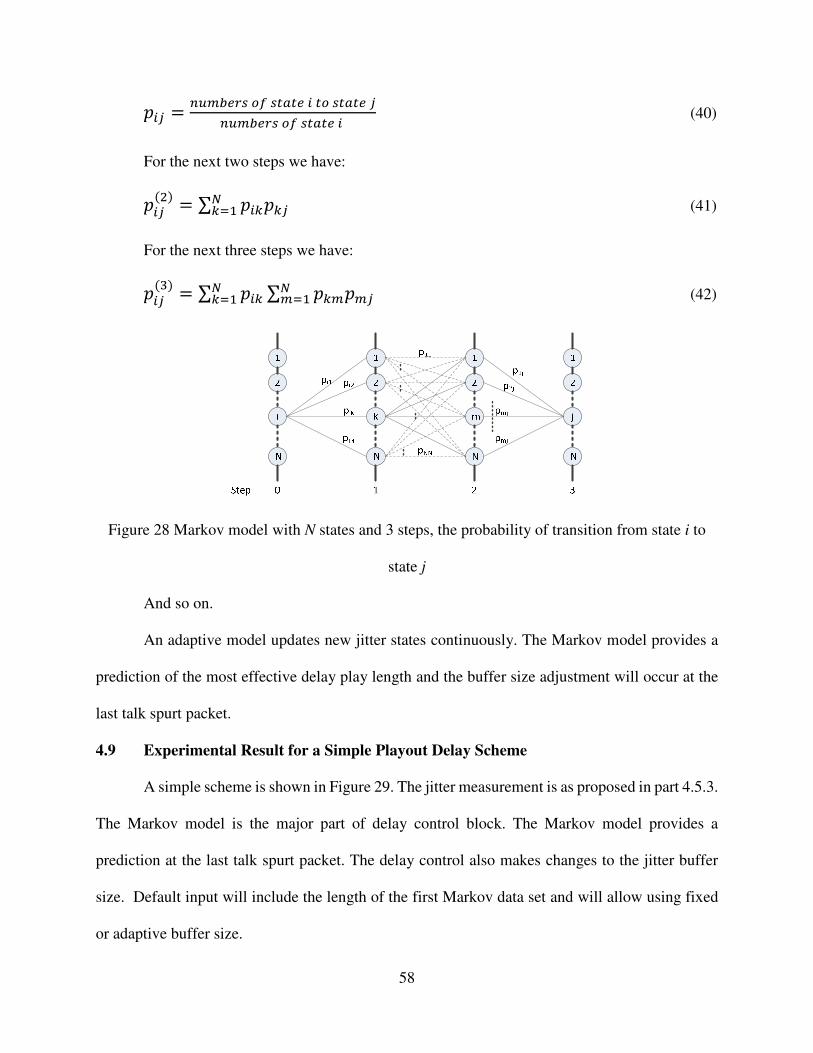
58
Q�© = -�( ¡¢� £ ��E�¡ � � ��E�¡ ©-�( ¡¢� £ ��E�¡ � (40)
For the next two steps we have:
Q�©(5) = ∑ Q�hQh©,h)� (41)
For the next three steps we have:
Q�©(|) = ∑ Q�h,h)� ∑ Qh(Q(©,()� (42)
Figure 28 Markov model with N states and 3 steps, the probability of transition from state i to
state j
And so on.
An adaptive model updates new jitter states continuously. The Markov model provides a
prediction of the most effective delay play length and the buffer size adjustment will occur at the
last talk spurt packet.
4.9 Experimental Result for a Simple Playout Delay Scheme
A simple scheme is shown in Figure 29. The jitter measurement is as proposed in part 4.5.3.
The Markov model is the major part of delay control block. The Markov model provides a
prediction at the last talk spurt packet. The delay control also makes changes to the jitter buffer
size. Default input will include the length of the first Markov data set and will allow using fixed
or adaptive buffer size.
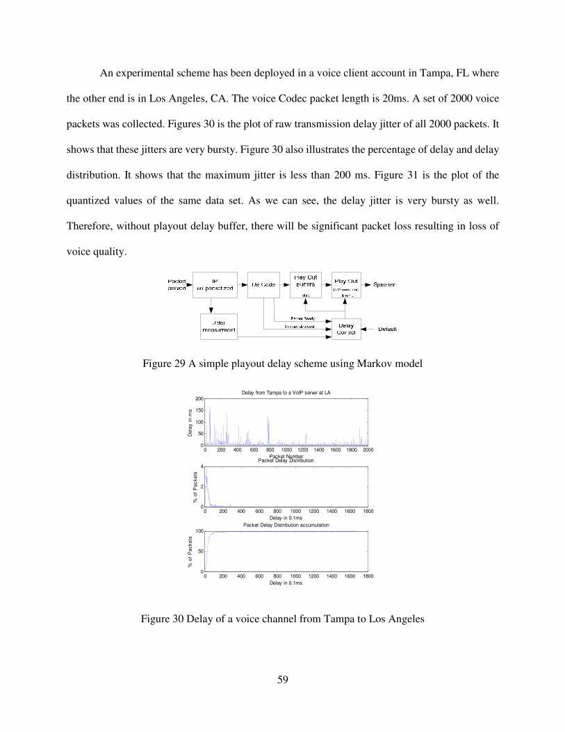
59
An experimental scheme has been deployed in a voice client account in Tampa, FL where
the other end is in Los Angeles, CA. The voice Codec packet length is 20ms. A set of 2000 voice
packets was collected. Figures 30 is the plot of raw transmission delay jitter of all 2000 packets. It
shows that these jitters are very bursty. Figure 30 also illustrates the percentage of delay and delay
distribution. It shows that the maximum jitter is less than 200 ms. Figure 31 is the plot of the
quantized values of the same data set. As we can see, the delay jitter is very bursty as well.
Therefore, without playout delay buffer, there will be significant packet loss resulting in loss of
voice quality.
Figure 29 A simple playout delay scheme using Markov model
Figure 30 Delay of a voice channel from Tampa to Los Angeles
0 200 400 600 800 1000 1200 1400 1600 1800 20000
50
100
150
200Delay from Tampa to a VoIP server at LA
Packet Number
De
lay
in
ms
0 200 400 600 800 1000 1200 1400 1600 18000
2
4Packet Delay Distribution
Delay in 0.1ms
% o
f P
ac
ke
ts
0 200 400 600 800 1000 1200 1400 1600 18000
50
100Packet Delay Distribution accumulation
Delay in 0.1ms
% o
f P
ac
ke
ts

60
Figure 32 is the transition matrix (after digitized) with two steps. Since the maximum jitter
is 10T, the Markov matrix is limited to 10th order. The pij is showing the probability of the jitter
length will be j.T (second) after 3.T (second) if current jitter is i.T (second). Visually we can see a
2T buffer size will be adequate.
Figure 31 Quantized delay of a voice channel from Tampa to Los Angeles
Figure 32 Transition matrix using two steps Markov model
0 200 400 600 800 1000 1200 1400 1600 1800 20000
5
10Delay Jitter from Tampa to a VoIP server at LA
Packet Number
Jitte
r x T
1 2 3 4 5 6 7 8 90
50
100Packet Delay Jitter Distribution
Jitter in numbers of frame legnth T
% o
f P
ackets
1 2 3 4 5 6 7 8 9 1097
98
99
100Packet Delay Jitter Distribution accumulation
Jitter in numbers of frame legnth T
% o
f P
ackets
0.98
0.90
0.83
0.80
0.83
1.00
1.00
0.00
1.00
0.01
0.05
0.00
0.00
0.00
0.00
0.00
1.00
0.00
0.00
0.00
0.00
0.00
0.00
0.00
0.00
0.00
0.00
0.00
0.05
0.00
0.00
0.00
0.00
0.00
0.00
0.00
0.00
0.00
0.00
0.00
0.17
0.00
0.00
0.00
0.00
0.00
0.00
0.00
0.00
0.00
0.00
0.00
0.00
0.00
0.00
0.00
0.17
0.00
0.00
0.00
0.00
0.00
0.00
0.00
0.00
0.00
0.00
0.00
0.00
0.00
0.00
0.00
0.00
0.00
0.00
0.20
0.00
0.00
0.00
0.00
0.00
j
i
1 2 3 4 5 6 7 8 9
1
2
3
4
5
6
7
8
9

61
There are few proposed playout delay buffer calculations [7],[8],[9], [10] which have been
applied from theory to practice. Typically, the Markov model will be applied to the client side,
which could be a small add-in application (app).
Applying two steps Markov model with limited states (ten), the computation complexity
has been reduced significantly (at least 90%). The playout delay is reduced by 40% compared to
fixed delay play out at the same packet loss rate, and the packet loss rate is reduced by 20% at the
same average fixed playout delay.
4.10 Playout Delay Decision and Analysis Based on Markov Model
The Markov model uses the past data for future prediction. Using a large data set could
lead to inaccurate prediction because the only up to date data could be used for the prediction due
to the random change of network condition. On the other hand, using small data set will reduce
the accuracy as well. Our experiment shows two seconds is sufficient. Expired data could become
noise and should be removed.
Per Markov, the expected next jitter state J based on current jitter state i will be as follows:
� = ∑ ªQ�©,©)� (43)
There were few issues with using the Markov model. The first problem is if pij= 0. That is
the state in which i only occurred once at the end. In that case, there will be no solution for the
next predicted jitter. However, in the playout delay control, there will be a solution. One of these
solutions is to keep the latest playout delay.
The second issue of using Markov model is similar to the first one. When there is no state
i in Markov model, the equation (40) will become infinity. In this case, the pij will be assigned to
zero.
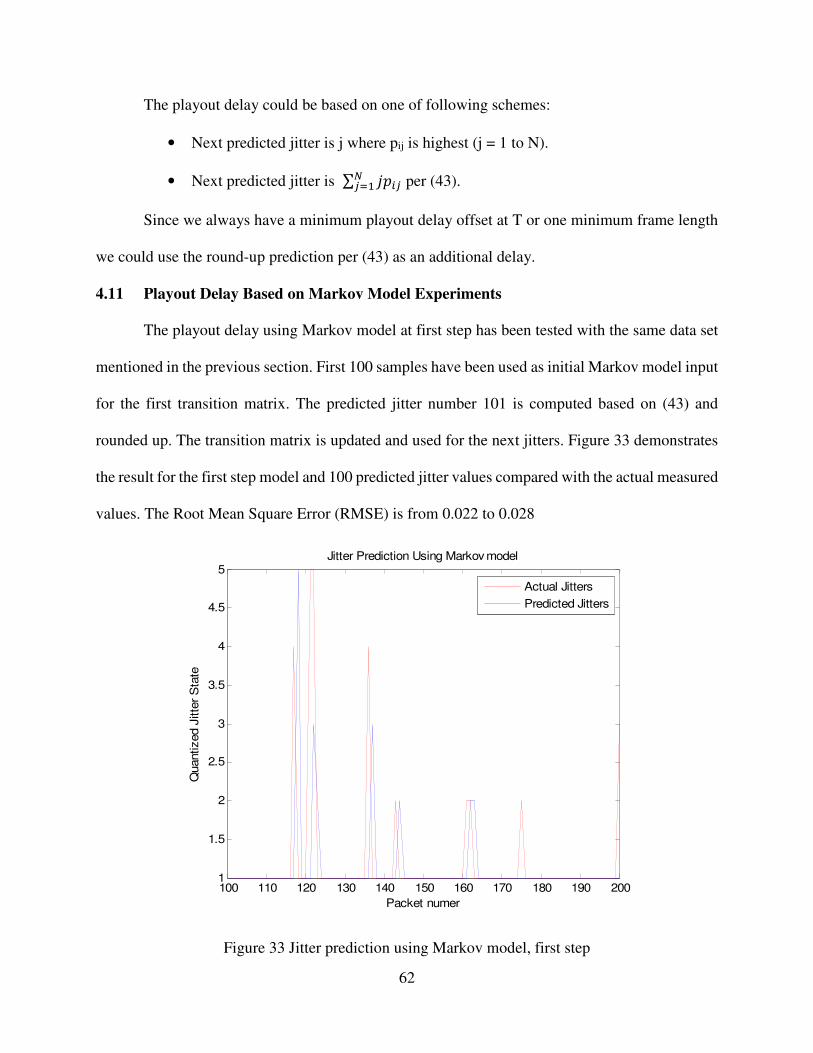
62
The playout delay could be based on one of following schemes:
• Next predicted jitter is j where pij is highest (j = 1 to N).
• Next predicted jitter is ∑ ªQ�©,©)� per (43).
Since we always have a minimum playout delay offset at T or one minimum frame length
we could use the round-up prediction per (43) as an additional delay.
4.11 Playout Delay Based on Markov Model Experiments
The playout delay using Markov model at first step has been tested with the same data set
mentioned in the previous section. First 100 samples have been used as initial Markov model input
for the first transition matrix. The predicted jitter number 101 is computed based on (43) and
rounded up. The transition matrix is updated and used for the next jitters. Figure 33 demonstrates
the result for the first step model and 100 predicted jitter values compared with the actual measured
values. The Root Mean Square Error (RMSE) is from 0.022 to 0.028
Figure 33 Jitter prediction using Markov model, first step
100 110 120 130 140 150 160 170 180 190 2001
1.5
2
2.5
3
3.5
4
4.5
5Jitter Prediction Using Markov model
Packet numer
Quantized J
itte
r S
tate
Actual Jitters
Predicted Jitters
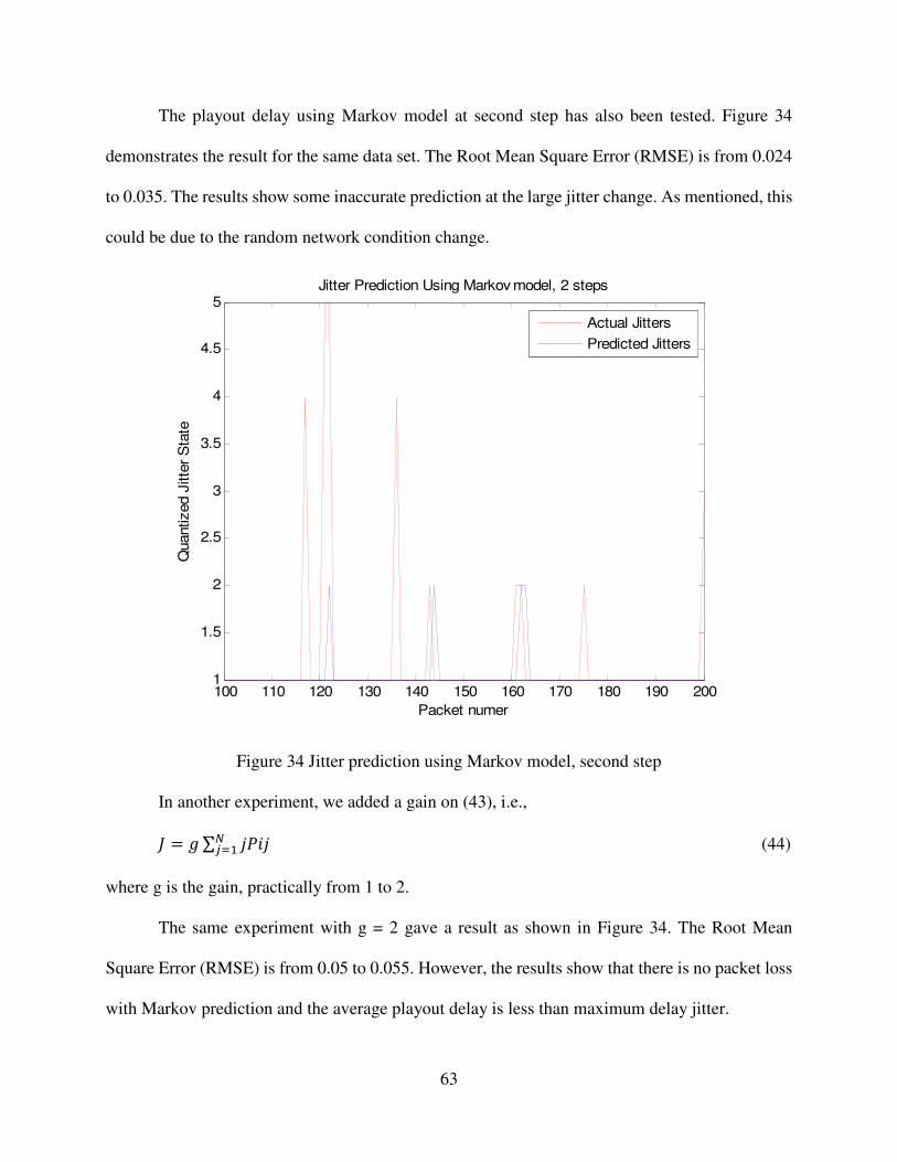
63
The playout delay using Markov model at second step has also been tested. Figure 34
demonstrates the result for the same data set. The Root Mean Square Error (RMSE) is from 0.024
to 0.035. The results show some inaccurate prediction at the large jitter change. As mentioned, this
could be due to the random network condition change.
Figure 34 Jitter prediction using Markov model, second step
In another experiment, we added a gain on (43), i.e.,
� = ∑ ªoPª,©)� (44)
where g is the gain, practically from 1 to 2.
The same experiment with g = 2 gave a result as shown in Figure 34. The Root Mean
Square Error (RMSE) is from 0.05 to 0.055. However, the results show that there is no packet loss
with Markov prediction and the average playout delay is less than maximum delay jitter.
100 110 120 130 140 150 160 170 180 190 2001
1.5
2
2.5
3
3.5
4
4.5
5Jitter Prediction Using Markov model, 2 steps
Packet numer
Quantized J
itte
r S
tate
Actual Jitters
Predicted Jitters
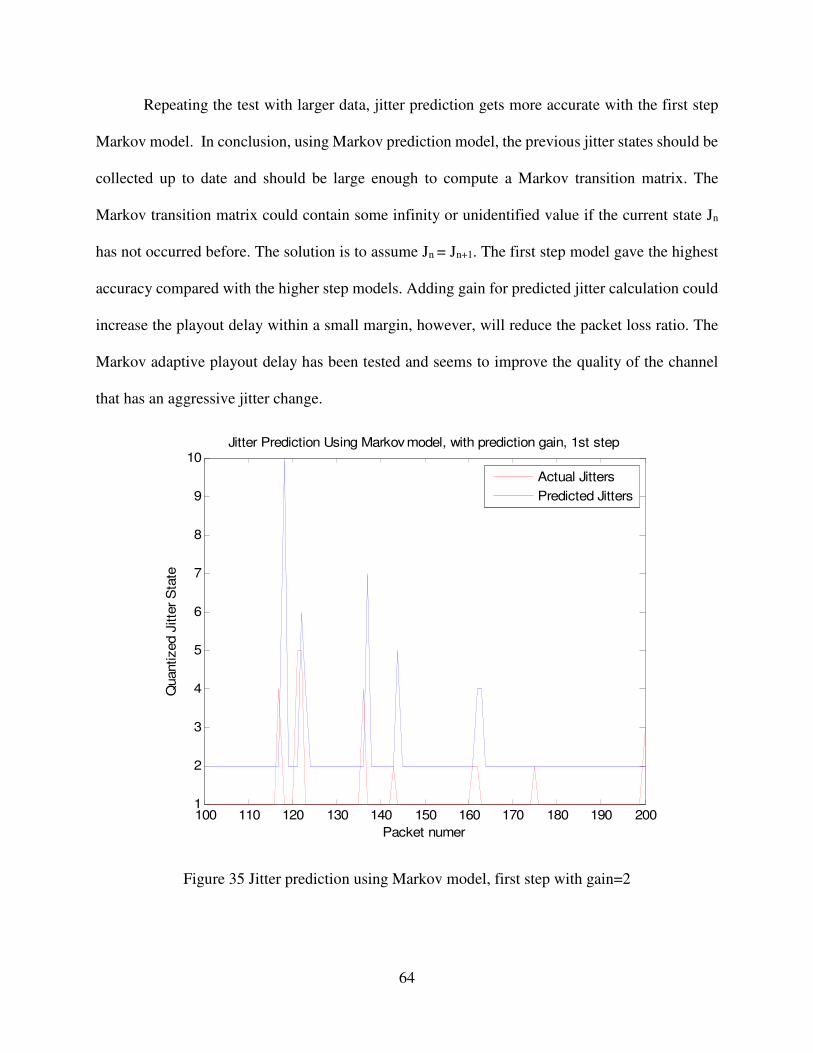
64
Repeating the test with larger data, jitter prediction gets more accurate with the first step
Markov model. In conclusion, using Markov prediction model, the previous jitter states should be
collected up to date and should be large enough to compute a Markov transition matrix. The
Markov transition matrix could contain some infinity or unidentified value if the current state Jn
has not occurred before. The solution is to assume Jn = Jn+1. The first step model gave the highest
accuracy compared with the higher step models. Adding gain for predicted jitter calculation could
increase the playout delay within a small margin, however, will reduce the packet loss ratio. The
Markov adaptive playout delay has been tested and seems to improve the quality of the channel
that has an aggressive jitter change.
Figure 35 Jitter prediction using Markov model, first step with gain=2
100 110 120 130 140 150 160 170 180 190 2001
2
3
4
5
6
7
8
9
10Jitter Prediction Using Markov model, with prediction gain, 1st step
Packet numer
Quantized J
itte
r S
tate
Actual Jitters
Predicted Jitters

65
4.12 Kalman Filter and Jitter Prediction Improvement
Recently, there have been a number of studies done on using Kalman filter for packet loss
improvement [11, 12,69-71]. The Kalman filter works as a tracking mechanism, improving the
next prediction based on previous prediction and measurement. The Kalman filter is used to reduce
the impact of noise on the input. The Kalman filtering is also used for delay compensation (playout
delay). Sirirat et al. [13] have proposed a Kalman filtering estimation. The linear dynamic process
is represented by a jitter model assuming a Gauss-Markov process autocorrelation. Comparing the
results of H. Bi et al. [71] with our results for the Markov model, it seems to be the same with Root
Mean Square Error (RMSE) from 0.022 to 0.035.
Kalman filter could be used with Markov prediction, where the Markov model will provide
the first prediction and the Kalman filter will provide updated prediction after receiving new
measurement. For future work, the study with the assumption that jitter is a Gaussian distribution
should be carried out as well.
Table 4 is a comparison of the improvement of R factor based on the same jitter data set
(2000 samples), between playout delay using adaptive Markov models, packet loss threshold and
fixed average jitter. The adaptive model gives the same packet loss ratio with packet loss threshold
model. However, average playout delay reduced significantly while the average jitter model has
more packet loss.
Table 4 Jitter playout delay improvement under R-factor
Adaptive Markov model
Packet loss threshold model
Average jitter model (Benchmark)
Theoretically performance N/A N/A N/A Empirical performance 88 80 65

66
CHAPTER 5: SUMMARY AND SUGGESTION FOR FUTURE RESEARCH
5.1 Summary
The VoIP quality is dependent on the network condition. Planning with a minimum
bandwidth is the first step of quality control. This involves changing the Codec, compressing or
simplifying IP header to reduce bandwidth in order to prevent traffic congestion and reduce the
impacts of packet loss. This research has analyzed the VoIP planning based on E-model and its
factors and has provided a simplified calculation for VoIP bandwidth.
A Method for calculating a limited duration (or a section) delay jitter without timestamp of
each packet and with variable Codec frame lengths has been proposed in this research. This will
be very useful in case the RTP header is being removed, which could close the gap in the
engineering solution for jitter delay prediction based on Markov model.
In order to deal with jitter as the major impact on network impairment, playout delay has
been used widely. The research has focused on optimized playout delay to improve the VoIP
quality. An approach using Markov prediction and quantized jitter has been proposed and tested.
The research has pointed out an important infinity loop in Markov model that has not been
addressed before. The research also included extensive tests and has confirmed that Markov has
8% improvement more than fixed threshold method and 28% more than average jitter method.
The Markov model seems to work better at the first step and could be more efficient if a prediction
gain is applied.

67
Future research could focus on Kalman filter and Markov autocorrelation models. Due to
the growth of the social network and smart grid, a social network study on the probability of a
voice call on the social network and the role of voice communication in smart grid also need further
study. Applying complex network on VoIP could be an interesting research area too.
5.2 A Maxell Model for Packet Loss Caused by Jitter
A packet loss is considered as a blocked packet during transportation. Dr. Thompson in his
book [72] stated that in Maxell model, a flux F at receiver sphere at Δt is zero for a blocked stream.
By increasing Δt F is greater than zero.
� = ∮ �X���∆�� (45)
where F is total packet received and K is receiver throughput.
In the future, research on all factors that relate to the flux could be an interesting road map.
Since not all factors are independent, i.e., Codec and jitter in combination could gain more effort
to block the packet.
5.3 VoIP and Social Network
The possibility of allowing a voice call from and to a social network is still under
investigation. The regulator and engineers should work closer to prepare a standard not just for the
voice quality but also for security. Today a telephone number could be an identity number while a
social network account is not. As soon as a social network account becomes an identity number,
telephony could be extended to the social network, and the regulation and standard will be changed
at that time to ensure improved quality.
5.4 Complex Network and VoIP
Recently, the development of Complex Network gives us another approach for VoIP study.
In the VoIP Complex Network, each node could be a hop and connection could be a link. Using

68
the node and its link as a property set, we could use a graph to simulate the VoIP behaviors and
estimate the quality of a call between two nodes [73].
5.5 Voice in Smart Grid
If voice becomes an add-in feature of a communication network, then there is a high
potential that VoIP will be embedded in the Smart Grid communication. Recently there are few
papers addressing this issue. Along with smart control and monitoring, smart voice communication
is also mentioned. The voice in Smart Grid deals with higher priority data communication to keep
its quality.

69
REFERENCES
[1] B. Goode, “Voice over Internet protocol (VoIP)”, Proceedings of the IEEE, vol. 90, pp.1495 – 1517, Sep. 2002.
[2] T. Daengsi and P. Wuttidittachotti, “VoIP quality measurement: Enhanced E-model using bias factor”, in Proc. IEEE Global Communications Conference (GLOBECOM), pp. 1329-1334, 2013.
[3] M. Soloducha, A. Raake, F. Kettler, N. Rohrer, E. Parotat, M. Waeltermann, S. Trevisany, and P. Voigt, “Towards VoIP quality testing with real-life devices and degradations “, in Proc. IEEE Speech Communication, pp. 1-5, 2016.
[4] M. Behdadfar, E. Faghihi, and M. E. Sadeghi, “QoS parameters analysis in VoIP network using adaptive quality improvement”, in Proc. IEEE Signal Processing and Intelligent Systems Conference (SPIS), pp. 73-77, Dec. 2015.
[5] H. Özer, İ. Avcıbaş, B. Sankur, and N. Memon, “Steganalysis of audio based on audio quality metrics,” TÜBİTAK Project 102E018, and Boğaziçi Research Fund project 01A20, http://www.busim.ee.boun.edu.tr/~sankur/SankurFolder/Audio_Steganalysis_16.doc.
[6] A. S. Spanias, “Speech coding: A tutorial review,” Proceedings of the IEEE, vol. 82, pp. 1541-1582, Oct 1994.
[7] B. Ngamwongwattana, “Sync & Sense Enable Adaptive Packetization VoIP”, Ph.D. Dissertation, University of Pittsburgh, 2007.
[8] S. Paulsen, T. Uhl, and K. Nowicki, “Influence of the jitter buffer on the quality of service VoIP”, in Proc. IEEE 3rd International Congress on Ultra Modern Telecommunications and Control Systems and Workshops (ICUMT), pp. 1-5, 2011.
[9] C. D. Nocito and M. S. Scordilis, “Monitoring jitter and packet loss in VoIP networks using speech quality features”, in Proc. IEEE Consumer Communications and Networking Conference (CCNC), pp. 685-686, 2011.
[10] B. H. Kim, H. Kim, J. Jeong, and J. Y. Kim, “VoIP receiver-based adaptive playout scheduling and packet loss concealment technique”, IEEE Transactions on Consumer Electronics, vol. 59, pp. 250-258, 2013.

70
[11] B. Oklander and M. Sidi, “Jitter buffer analysis”, in Proc. IEEE 17th International Conference on Computer Communications and Networks (ICCCN), pp. 1-6, 2008.
[12] P. K. Jawahar, D. EgfinNirmala, and V. Vaidehi, “Qos enhancement in wireless VoIP networks using interactive multiple model based Kalman filter”, in Proc. IEEE 2nd International Conference on Advanced Computing (ICoAC), pp. 19-25, 2010.
[13] S. R. Miralavi, S. Ghorshi, and A. Tahaei, “Kalman filter based packet loss replacement in presence of additive noise”, in Proc. 25th IEEE Canadian Conference on Electrical and Computer Engineering (CCECE), pp. 1-4, 2012.
[14] M. Pohjola and H. Koivo, "Measurement delay estimation for Kalman filter in network control system", in Proc. 17th International Federation of Automatic Control (IFAC) World Congress, pp. 4192-4197, 2008.
[15] IETF Internet Protocol website https://tools.ietf.org/html/rfc1180
[16] Internet Protocol Specification, “http://www.rfc-editor.org/ien/ien41.pdf”
[17] V. N. G. J. Soares, P. A. C. S. Neves, and J. J. P. C. Rodrigues, “Past, present and future of IP telephony”, in Proc. IEEE International Conference on Communication Theory, Reliability, and Quality of Service, pp. 19-24, 2008.
[18] A. G. Nascimento, E. Mota, S. Queiroz, L. Galvao, and E. Nascimento, “Towards an efficient header compression scheme to improve VoIP over wireless mesh networks”, in Proc. IEEE Symposium on Computers and Communications (ISCC), pp. 170-175, 2009.
[19] B. Hung, D. Defrancesco, B. Cheng, and P. Sukumar, “An evaluation of IP header compression on the GIG joint IP modem system”, in Proc. IEEE Military Communications Conference (MILCOM), pp. 1484-1490, 2014.
[20] H. Zhang, M. Boutabia, H. Nguyen, and L. Xia, “Field performance evaluation of VoIP in 4G trials”, in Proc. IEEE International Conference on Multimedia and Expo (ICME), pp. 1-4, 2011.
[21] S. Alfredsson, A. Brunstrom, and M. Sternad, “Impact of 4G wireless link configurations on VoIP network performance”, in Proc. IEEE International Symposium on Wireless Communication Systems (ISWCS), pp. 708-712, 2008.
[22] M. S. Mushtaq, S. Fowler, B. Augustin, and A. Mellouk, “QoE in 5G cloud networks using multimedia services”, in Proc. IEEE Wireless Communications and Networking Conference (WCNC), pp. 1-6, 2016.

71
[23] S. Kharche and A. Mahajan, “IPv4 and IPv6 performance comparison for simulated DNS and VoIP traffic in Windows 2007 and Windows 2008 client server environment”, in Proc. IEEE World Congress on Information and Communication Technologies, pp. 408-412, 2012.
[24] O. J. S. Parra, A. P. Rios, and G. L. Rubio, “Quality of service over IPV6 and IPV4”, in Proc. IEEE 7th International Conference on Wireless Communications, Networking and Mobile Computing (WiCOM), pp. 1-4, 2011.
[25] D. A. Melnikov, Y. N. Lavrukhin, A. P. Durakovsky, V. S. Gorbatov, and V. R. Petrov, “Access control mechanism based on entity authentication with IPv6 header "flow label" field”, in Proc. IEEE 3rd International Conference on Future Internet of Things and Cloud (FiCloud), pp. 158-164, 2015.
[26] E. Antwi-Boasiako, E. Kuada, and K. Boakye-Boateng, “Role of Codec selection on the performance of IPsec secured VoIP”, in Proc. International Conference on Advances in Computing, Communications and Informatics (ICACCI), pp. 2508-2514, 2016.
[27] P. P. Vaidyanathan, “Generalizations of the sampling theorem: Seven decades after Nyquist”, IEEE Transactions on Circuits and Systems I: Fundamental Theory and Applications, vol. 48, no. 9, pp. 1094-1109, Sep. 2001.
[28] Q. Wang and S. Chen, “A low power prediction SAR ADC integrated with DPCM data compression feature for WCE application”, in Proc. IEEE Biomedical Circuits and Systems Conference (BioCAS), pp. 107-110, 2016.
[29] Y. Yatsuzuka, S. Iizuka, and T. Yamazaki, “A variable rate coding by APC with maximum likelihood quantization from 4.8 kbits/s to 16 kbits/s”, in Proc. IEEE International Conference on Acoustics, Speech, and Signal Processing (ICASSP), pp. 3071-3074, 1986.
[30] G. A. Haidar; R. Achkar, and H. Dourgham, “A comparative simulation study of the real effect of PCM, DM and DPCM systems on audio and image modulation”, in Proc. IEEE International Multidisciplinary Conference on Engineering Technology (IMCET), pp. 144-149, 2016.
[31] Z. H. Perić, M, Tančić, S. S. Tomić, and D. G. Ćirić, “Subband coding of audio signal with logarithmic companders”, in Proc. IEEE 12th International Conference on Telecommunication in Modern Satellite, Cable and Broadcasting Services (TELSIKS), pp. 19-22, 2015.
[32] K. H. Chou and C. P. Chung, “Predictive mode selection of adaptive transform coding with rate-distortion optimization for MPEG-4 part-10 AVC/H.264”, in Proc. IEEE 6th International Conference on Information Communication and Management (ICICM), pp. 233-238, 2016.

72
[33] H. Kaneko and T. Sekimoto, “Logarithmic PCM encoding without diode compander”, IEEE Transactions on Communications Systems, vol. 11, no. 3, pp. 296-307, Sep. 1963.
[34] S. Moller and J. Berger, “Describing telephone speech codec quality degradations by means of impairment factors,” J. Audio Eng. Soc., vol. 50, pp. 667-680, Sep. 2002.
[35] L. Hanzo, C. Somerville, and J. Woodard, “Linear predictive vocoder”, in Proc. IEEE Voice and Audio Compression for Wireless Communications, pp. 565-579, 2007.
[36] R. Jage and S, Upadhya, “CELP and MELP speech coding techniques”, in Proc. IEEE International Conference on Wireless Communications, Signal Processing and Networking (WiSPNET), pp. 1398-1402, 2016.
[37] S. M. El Noubi, M. El-Said Nasr, and E. S. Gemeay, “Performance of analysis-by-synthesis low-bit rate speech coders in mobile radio channel”, in Proc. IEEE 19th National Radio Science Conference, pp. 363-371, 2002.
[38] R. Salami, L. Hanzo, R. Steele, K. Wong, and I. Wassell, “Speech Coding”, in Mobile Radio Communications, R. Steele and L. Hanzo, Eds., Piscataway, NJ; IEEE Press, pp. 186-346, 1999.
[39] K. Seto and T. Ogunfunmi, “Scalable multi-rate iLBC”, in Proc. IEEE International Symposium on Circuits and Systems (ISCAS), pp. 1034-1037, 2012.
[40] P. Srivastava, K. Babu, and T. Osv, “Performance evaluation of Speex audio Codec for wireless communication networks”, in Proc. IEEE Eighth International Conference on Wireless and Optical Communications Networks (WOCN), pp. 1-5, 2011.
[41] J. Srinonchat, “New technique to reduce bit rate of LPC-10 speech coder”, in Proc. IEEE Region 10 Conference (TENCON), pp. 1-4, 2006.
[42] S. K. Pedram, S. Vaseghi, B. Langari, “Audio packet loss concealment using spectral motion”, in Proc. IEEE International Conference on Acoustics, Speech and Signal Processing (ICASSP), pp. 6707-6710, 2014.
[43] L. F. Gallardo, “A paired-comparison listening test for collecting voice likability scores”, in Proc. Speech Communication, ITG Symposium, pp. 1-5, 2016.
[44] L. Angrisani, D. Capriglione, L. Ferrigno, and G. Miele, “Measurement of the IP packet delay variation for a reliable estimation of the mean opinion score in VoIP services”, in Proc. IEEE International Instrumentation and Measurement Technology Conference (I2MTC), pp. 1-6. 2016.
73
[45] O. Jukić and I. HeĐi, “PSQM - Platform for service quality management”, in Proc. IEEE 36th International Convention on Information and Communication Technology, Electronics and Microelectronics (MIPRO), pp. 371-375, 2013
[46] E. Akdemir, “Spectral distance measures for matching consecutive speech segments”, in Proc. IEEE 21st Signal Processing and Communications Applications Conference (SIU), pp. 1-4, 2013.
[47] J. C. Rutledge, K. E. Cummings, D. A. Lambert, and M. A. Clements, “Synthesizing styled speech using the Klatt synthesizer”, in Proc. IEEE International Conference on Acoustics, Speech, and Signal Processing (ICASSP), pp. 648-651, 1995.
[48] D.H. Klatt, “A digital filter bank for spectral matching,” in Proc. IEEE International Conference on Acoustics, Speech, and Signal Processing (ICASSP), pp. 573-576, Apr. 1976.
[49] S. Voran, “Objective estimation of perceived speech quality .II. Evaluation of the measuring normalizing block technique”, IEEE Transactions on Speech and Audio Processing, vol. 7, no. 4, pp. 383-390, Jul. 1999.
[50] E. Myakotnykh, “Adaptive speech quality in Voice-over-IP communication” Ph.D.
Dissertation, University of Pittsburgh, 2008.
[51] T. Daengsi, and P. Wuttidittachotti, “QoE modeling: A simplified e-model enhancement using subjective MOS estimation model”, in Proc. IEEE Seventh International Conference on Ubiquitous and Future Networks, pp. 386-390, 2015.
[52] Cisco, “IP telephony/Voice over IP”, http://www.cisco.com/en/US/tech/tk652/tk701/tsd_technology_support_protocol_home.html
[53] P. P. Kadam, Z. Saquib, and A. Lahane, “Adaptive echo cancellation in VoIP network”, in Proc. IEEE International Conference on Engineering and Technology (ICETECH), pp. 295-299, 2016.
[54] R. Sankar and A. T. Le, “Voice over IP (VoIP) Quality of Service (QoS) Monitoring”, Technical Report, Florida High Tech Corridor, 2011.
[55] D. Arifianto and T. R. Sulistomo, “Subjective evaluation of voice quality over GSM network for quality of experience (QoE) measurement”, in Proc. IEEE International Symposium on Intelligent Signal Processing and Communication Systems (ISPACS), pp. 148-152, 2015.

74
[56] F. Jalalinajafabadi, C. Gadepalli, M. Ghasempour, M. Luján, B. Cheetham, and J. Homer, “Computerised objective measurement of strain in voiced speech”, in Proc. IEEE 37th Annual International Conference of the IEEE Engineering in Medicine and Biology Society (EMBC), pp. 5589-5592, 2015.
[57] ITU-T G.107: The E-model: a computational model for use in transmission planning https://www.itu.int/rec/T-REC-G.107
[58] P. Galiotos, T. Dagiuklas, and D. Arkadianos, “QoS management for an enhanced VoIP platform using R-factor and network load estimation functionality”, in Proc. 5th IEEE International Conference on High Speed Networks and Multimedia Communication (Cat. No.02EX612), pp. 305-314, 2002.
[59] Cisco, VoIP call admission control, http://www.cisco.com/c/en/us/td/docs/ios/solutions_docs/voip_solutions/CAC.html
[60] ITU E-Model tool, http://www.itu.int/ITU-T/studygroups/com12/emodelv1/calcul.php
[61] M. G. Hluchyj and M. J. Karol, “Queueing in high-performance packet switching”, IEEE
Journal on Selected Areas in Communications, vol. 6, no.9, pp. 1587-1596, Dec. 1988.
[62] F. Huebner, D. Liu, and J. M. Fernandez, “Queueing performance comparison of traffic models for Internet traffic”, in Proc. IEEE Global Telecommunications Conference (GLOBECOM), pp. 471 – 476, 1998.
[63] Q. Gong and P. Kabal, “A new optimum jitter protection for conversational VoIP”, in Proc. IEEE International Conference on Wireless Communications and Signal Processing (WCSP), pp. 1-5, 2009.
[64] M. Baratvand, M. Tabandeh, A. Behboodi, and A. F. Ahmadi, “Jitter-buffer management for VoIP over wireless LAN in a limited resource device”, in Proc. IEEE 4th International Conference on Networking and Services (ICNS), pp. 90-95, 2008.
[65] K. M. McNeill, M. Liu, and J. J. Rodriguez, “An adaptive jitter buffer play-out scheme to improve VoIP quality in wireless networks", in Proc. IEEE Military Communications Conference (MILCOM), pp. 1-5, 2006.
[66] C. Soria-López and R. V. M. Ramos, “Applying traditional VoIP playout delay control algorithms to MANETs”, in Proc. IEEE 8th International Caribbean Conference on Devices, Circuits, and Systems (ICCDCS), pp. 1-4, 2012.
[67] M. K. Ishak, G. Herrmann, and M. Pearson, “Performance evaluation using Markov model for a novel approach in Ethernet based embedded networked control communication”, in Proc. IEEE Systems Conference (SysCon), pp. 1-7, 2016.

75
[68] X. Zhang and K.G. Shin, “Markov-chain modeling for multicast signaling delay analysis”, IEEE/ACM Transactions on Networking, vol. 12, no. 4, pp. 667 – 680, Aug. 2004.
[69] V. Tzvetkov, “SIP registration optimization in mobile environments using extended Kalman filter”, in Proc. IEEE 3rd International Conference on Communications and Networking in China (ChinaCom), pp. 106-111, 2008.
[70] E. F. Costa and B. de Saporta, “Precomputable Kalman-based filter for Markov jump linear systems”, in Proc. IEEE 3rd Conference on Control and Fault-Tolerant Systems (SysTol), pp. 393-398, 2016.
[71] H. Bi, J. Ma, and F. Wang, “An improved particle filter algorithm based on ensemble Kalman filter and Markov chain Monte Carlo method”, IEEE Journal of Selected Topics in Applied Earth Observations and Remote Sensing, vol. 8, no. 2, pp. 447-458, Feb. 2015.
[72] R. A. Thompson, “A Fifth Generation of Global Ubiquitous Networks”, Chapter 4, Springer, 2017.
[73] A. T. Le and R. Sankar, “Complex Network Approach for Power Grids Vulnerability and Large Area Blackout”, in Proc. 5th International Conference on Computational Social Networks, pp. 206-213, Aug 2016.
[74] C. D. Nocito and M. S. Scordilis, “Monitoring jitter and packet loss in VoIP networks using speech quality features”, in Proc. IEEE Consumer Communications and Networking Conference (CCNC), pp. 685 – 686, 2011.
[75] Y. Han, D. Magoni, P. McDonagh, and L. Murphy, “Determination of bit-rate adaptation
thresholds for the Opus Codec for VoIP services”, in Proc. IEEE Symposium on Computers and Communications (ISCC), pp. 1-7, Jun. 2014.
[76] K. Tseng, Y. Lai, and Y. Lin, ‘Perceptual codec and interaction aware playout algorithms and quality measurements for VoIP systems”, IEEE Transactions on Consumer Electronics, vol. 50, no. 1, pp. 297–305, Jan. 2004.
[77] T. Daengsi, K. Yochanang, and P. Wuttidittachotti, “A study of perceptual VoIP quality evaluation with Thai users and Codec selection using voice quality - Bandwidth tradeoff analysis”, in Proc. International Conference on ICT Convergence (ICTC), pp. 691-696, 2013.
[78] D. Luksa, S. Fajt, and M. Krhen, “Sound quality assessment in VOIP environment’, in Proc. 37th International Convention on Information and Communication Technology, Electronics and Microelectronics (MIPRO), pp. 1066-1070, 2014.
[79] E. Faghihi, M. Behdadfar, and M. E. Sadeghi, “Sender based adaptive VoIP quality improvement using constructive feedback”, in Proc. 7th Conference on Information and Knowledge Technology (IKT), pp. 1-6, 2015.
76
[80] N. S. Jayant, “Digital coding of speech waveforms: PCM, DPCM, and DM quantizers,” Proceedings of the IEEE, vol. 62, no. 5, pp. 611-632, May 1974.
[81] J. Kang, Y. Kang, I. Na, Y. Choi, and J. Kim; “A study of subjective speech quality measurement over VoIP network”, in Proc. IEEE International Conferences on Info-Tech and Info-Net, vol. 5, pp. 311-316, 2001.
[82] DYNASTAT, “Summary of Speech Intelligibility Testing Methods,” http://www.dynastat.com/SpeechIntelligibility.htm
[83] Online resource: Speech Quality and Evaluation http://www.acoustics.hut.fi/publications/files/theses/lemmetty_mst/chap10.html
[84] O. Hersent, J-P. Petit, and D. Gurle, Beyond VoIP protocols: Understanding voice technology and networking techniques for IP telephony, Willey, pp. 79-81, 2015
[85] R. E. Crochiere, J. M. Tribolet, and L. R. Rabiner, “An interpretation of the log likelihood ratio as a measure of waveform coder performance,” IEEE Transactions on Acoustics, Speech, and Signal Processing, vol. ASSP-28, no.3, pp. 318-323, June 1980.
[86] D. Chow and W. H. Abdulla, “Speaker Identification Based on Log Area Ratio and Gaussian Mixture Models in Narrow-Band Speech,” http://www.ece.auckland.ac.nz/~wabd002/pricai.pdf.
[87] P. Chu and D. Messerschmitt, “Frequency weighted linear prediction”, in Proc. IEEE International Conference on Acoustics, Speech, and Signal Processing (ICASSP), vol. 7, pp. 1318-1321, 1982.
[88] A. H. Gray, Jr. and J. D. Markel “Distance measures for speech processing,” IEEE Transactions on Acoustics, Speech, and Signal Processing, vol. ASSP-28, no. 4, pp. 380-391, Oct. 1976.
[89] Y. Tohkura, “A weighted cepstral distance measure for speech recognition,” IEEE Transasctions on Signal Processing, vol. 35, no. 10, pp. 1414 – 1422, Oct. 1987.
[90] S. Wang, A. Sekey, and A. Gersho, “An objective measure for predicting subjective quality of speech coders,” IEEE Journal on Selected Areas in Communications, vol. 10, no. 5, pp. 819-829, Jun. 1992.
[91] W. Yang, M. Benbouchta, and R. Yantomo, “Performance of the modified Bark spectral distortion as an objective speech quality measure,” in Proc. IEEE International Conference on Acoustics, Speech, and Signal Processing (ICASSP), vol. 1, pp. 541-544, May 1998.
[92] W. Yang, M. Dixon, and R. Yantorno, “A modified bark spectral distortion measure which uses noise masking threshold,” IEEE Speech Coding Workshop, pp. 55-56, Sep 1997.

77
[93] W. Yang, “Enhanced modified bark spectral distortion (EMBSD): an objective speech quality measure based on audible distortion and cognition model”, Doctorate Thesis, Temple University, PA, 1999.
[94] T. Thiede and E. Kabot, “A new perceptual quality measure for bit rate reduced audio,” http://www.mp3-tech.org/programmer/docs/AES1996Copenhagen.pdf
[95] T. Painter and A. Spanias, “Perceptual coding of digital audio”, Proceedings of the IEEE, vol. 88, no. 4, pp. 451 – 515, Apr. 2000.
[96] End-to-end speech quality assessment of networks using PESQ (P.862) http://www.itu.int/itudoc/itu-t/workshop/qos/pesq/s6p2b.pdf
[97] A. W. Rix , J. G. Beerends, M. P. Hollier, and A.P. Hekstra, “Perceptual evaluation of speech quality (PESQ)-a new method for speech quality assessment of telephone networks and Codecs”, in Proc. IEEE International Conference on Acoustics, Speech, and Signal Processing (ICASSP), vol. 2, pp. 749-752, 2001.
[98] D. H. Klatt, “Prediction of perceived phonetic distance from critical-band spectra: A first step”, in Proc. IEEE International Conference on Acoustics, Speech, and Signal Processing (ICASSP), pp.1278 – 1281, 1982.
[99] L. Ding and R. A. Goubran, “Speech quality prediction in VoIP using the extended E-model", in Proc. IEEE Global Telecommunications Conference (GLOBECOM), pp. 3974-3978, 2003.
[100] A. S. Acampora, An Introduction to Broadband Networks, NY: Plenum Press, 1994.
[101] P. G. Harrison and Y. Zhang, “Delay analysis of priority queues with modulated traffic”, in Proc. 13th IEEE International Symposium on Modeling, Analysis, and Simulation of Computer and Telecommunication Systems, pp. 280-287, 2005.
[102] L. Zheng and L. Zhang, “Modeling and performance analysis for IP traffic with multi-class QoS in VPN”, in Proc. IEEE 21st Century Military Communications Conference Proceedings (MILCOM), vol. 1, pp. 330-334, 2000.
[103] B. Klepec and A. Kos, “Performance of VoIP applications in a simple differentiated services network architecture”, in Proc. International Conference on Trends in Communications (EUROCON), vol. 1, pp. 214-217, 2001.
[104] L. Xin, W. Ke, and D. Huijing, “Wavelet multifractal modeling for network traffic and queuing analysis”, in Proc. International Conference on Computer Networks and Mobile Computing, pp. 260-265, 2001.
78
[105] F. Gotoh and S. Uno, “User modeling and uplink scheduling in IP-based ITS network”, Proc. IEEE 53rd Vehicular Technology Conference (VTC), vol. 4, pp. 3027-3031, Spring 2001.
[106] C. Hu, X. Chen, W. Li, and B. Liu, “Fixed-Length Switching vs. Variable-length Switching in Input-Queued IP Switches”, in Proc. IEEE Workshop on IP Operations and Management, pp. 117-122, 2004.
[107] S. -Q. Li and J. Mark, “Performance of Voice/Data Integration on a TDM System”, IEEE Transactions on Communications, vol. 33, no. 12, pp. 1265-1273, Dec. 1985.
[108] J. E. Flood, Telecommunications Switching, Traffic and Networks, Chapter 4: Telecommunications Traffic, NY: Prentice-Hall, 1998.
[109] Richard Parkinson, “Traffic Engineering Techniques in Telecommunications”, http://www.tarrani.net
[110] M. J. Neely and E. Modiano, “Logarithmic delay for N × N packet switches”, in Proc. IEEE Workshop on High Performance Switching and Routing, pp. 1-7, Apr. 2004.
[111] W. Wang, S. C. Liew, Q. Pang, and V. O. K. Li, “A multiplex-multicast scheme that improves system capacity of voice-over-IP on wireless LAN”, in Proc. 9th International Symposium on Computers and Communications (ISCC), pp. 472-477 vol. 1, 2004.
[112] A. Hussian, K. Sobraby, and M. A. Ali, “A novel two-queue model for ATM networks”, in Proc. IEEE Global Telecommunications Conference (GLOBECOM), vol. 2, pp. 758-765, 1997.
[113] S. Shankar, J. del Prado Pavon, and P. Wienert, “Optimal packing of VoIP calls in an IEEE 802.11 a/e WLAN in the presence of QoS constraints and channel errors”, Proc. IEEE Global Telecommunications Conference (GLOBECOM), vol. 5, pp. 2974-2980, 2004.
[114] K. Lan and T. Wu, "Evaluating the perceived quality of infrastructure-less VoIP", in Proc. IEEE International Conference on Multimedia and Expo (ICME), pp. 1-6, 2011.