www.SandV.com6 SOUND & VIBRATION/OCTOBER 2013

Many different multi-exciter configurations have been created to produce motion in six degrees-of-freedom (6-DOF) simultane-ously. This article examines some of these configurations and gives examples of controlling one popular setup, using advanced MIMO (multiple-input and multiple-output) control. Several types of problems were encountered with each configuration, and pos-sible causes and suggested remedies are presented.

For many years, aerospace companies, government organiza-tions, universities, testing houses and test engineers have conceived various ways to configure multiple exciters to create simultaneous multi-degree-of-freedom (MDOF) motion. One of the earliest 3-DOF arrangements, which is shown in Figure 1, was conceived in 1958.

The goal was to create true vector motion to simulate missile flight environments on control electronics modules. Al Crobaugh and Fred Sheets, at the White Sands Proving Ground in New Mexico, developed the arrangement shown in Figure 1 in 1958. An aluminum block was supported on a (horizontal) oil film, on top of a vertical shaker. Horizontal and lateral shakers were “at-tached” to the block through vertical plates that had a thin oil film supplied via gravity to a groove cut into each plate about an inch from the plate edges.

At low frequencies and low displacements, the system worked remarkably well. However, if the motion exceeded 1 g, or the test article created a moment about one of the axes, the plates would separate from the block. So the system proved to be impractical, but it certainly sparked a lot of interest in MDOF testing more than 50 years ago. Since then, the more ambitious goal of true MDOF testing has involved creating and controlling 6-DOF motion using a variety of test configurations.

This article covers several examples of popular actuation systems that use various configurations to excite test articles in six DOF and also their respective performance characteristics. Each of the discussed configurations is named in what follows according to the number of actuators in each translational DOF: X, Y and Z.

One of these will be examined in detail, which is called the 2-2-4 configuration. We discuss test data that shows its performance characteristics, types of problems that are encountered with its use, how these test results can serve as a guide to identify possible causes, and how these results can be used to determine remedies.

We will be using the term over-actuated to discuss those 6-DOF configurations where more actuators than desired rigid body DOFs are employed. When 6-DOF test systems are over-actuated, then bending of the test platform can occur if the configuration’s actua-tors are driven independently. So to avoid bending, the drives need to be linearly dependent. This dependency needs to be enforced by a controller through an output transformation.1,2

A simple example of an over-actuated configuration is a beam supported by three actuators that are attached to the beam at each end, with the third actuator attached at its mid-point (Figure 2). This system can create motion in two rigid-body DOFs: pure Z and rotation (about Y) centered at the (hinged) attachment of the center actuator. Driving the center actuator independently of the two end actuators results in bending the beam, which is the flexible-body DOF. The three actuator drives need to be linearly dependent during a vibration test to avoid bending the beam; e.g., all three drives the same for pure Z and the end two actuators driven out of phase for rotation about Y, while the center actuator is driven with zero drive. A properly chosen output transformation can be defined that can enforce this interdependence between drives and avoid bending the beam.1,2

As we add more actuators, the degree of over-actuation increases.

This increases the complexity of the possible flexible-body DOFs and its associated output transformation.1,2 Over-actuation is similar to the concept of statically determinate and statically in-determinate that we find in structural mechanics.

6-DOF Excitation SystemsA. 4-4-4 configuration shown in Figure 3 has four actuators point-

ing in each direction, X, Y and Z. It is over-actuated, with six rigid-body and six flexible-body DOFs possible.

B. 1-2-3 configuration shown in Figure 4 has one actuator along X, 2 along Y and 3 along Z. This scheme is in heavy use due to its simplicity. It is not over-actuated, so there are no flexible-body DOFs that can be actuated to cause bending.

C. 2-2-2 configuration shown in Figure 5 has two actuators point-ing in each direction, X, Y and Z. Each pair of actuators can also actuate moments along RX, RY, and RZ. This configuration is also not over-actuated.

Note that each of the previous configurations has a different set of trade-offs. To simplify the following discussion, we will focus our discussion on the following 2-2-4 configuration, since this arrangement of actuators is popular and is currently used in many MDOF designs. As a result, 2-2-4 will be discussed in more detail to show examples of what these trade-offs might be in typical applications.

D. 2-2-4 configuration shown in Figure 6 has two actuators pointing in each of X and Y, and four pointing in Z. This configuration is over-actuated horizontally and vertically and can create six

Controlling 6-DOF Systems with Multiple ExcitersRussell Ayres, Marcos A. Underwood, and Tony Keller, Spectral Dynamics, Inc., San Jose, California

Figure 1. XYZ shaker arrangement, circa 1958.

Figure 2. Three-shaker over-actuated system with two rigid-body and one flexible-body DOFs.

Z Y

X

www.SandV.com DYNAMIC TESTING REFERENCE ISSUE 7

rigid-body and two flexible-body DOFs. The rigid-body DOFs are vertical (Z), horizontal (X), and lateral (Y) translation: roll (Rx), pitch (Ry) and yaw (Rz) rotation. The flexible DOFs are vertical and horizontal torsion. For example, if the four vertical shakers are driven out of phase with respect to each other, as we successively go counter-clockwise from Z1 to Z4, we will be applying a torsion load to the table. If the four horizontal shakers are also so driven out of phase with respect to each other, then we will be applying a shear load to the table, i.e., horizontal torsion.

Multiple-Exciter Control SystemsAs multiple degree-of-freedom shaker arrangements have

evolved, so too have multiple-exciter control systems. The state-ment “Multi-exciter testing is not for the faint of heart” has proven

to be quite true. At the same time, the continuing development of multi-shaker control technology, as documented in the references shown at the end of this article, have permitted ever more accurate and successful results as test requirements evolve.

Initially, multi-shaker control algorithms were based on square control, where the number of control transducers is equal to the number of exciters.3,4 As test concepts evolved, it became obvious that conditions existed where more control points than exciters may improve our control accuracy, so rectangular control was developed.5 If it is desired to control 6 degrees-of-freedom with eight exciters, a “transformation” to and from the number of excit-ers and control transducers to the six DOFs is required. Today this is accomplished with software coordinate transformations.1,2 An input transformation is then used to map the response at the control transducers to its 6-DOF representation, and an output transforma-tion is used to map the 6-DOF drives to the actual actuator drives.

When using the 2-2-4 configurations, several rules of thumb have

Figure 3. Six-DOF testing with 12 exciters – four vertical, four horizontal and four lateral.

Y1 X1

Z1Y2

X2

Z2

X3 Y3

Z3

X4

Y4

Z4

4-4-4

Figure 4. Six-DOF testing with six exciters – three vertical, two horizontal and one lateral.

X1

Z1Y2

Z2

Z3

Y1

1-2-3

Figure 5. Six-DOF testing with six exciters – two vertical, two horizontal and two lateral.

Y1

X1

Z1X2

Z2

Y2

2-2-2

Figure 7. Customer-assembled six-DOF system using 2-2-4 configuration.

Figure 8. Table bottom view showing stinger attachments.

Figure 6. Multiple-DOF testing with eight exciters – four vertical, two hori-zontal and two lateral.

X1

Z1Y2

Z2

X2

Z3

Y1

Z4

2-2-4

www.SandV.com8 SOUND & VIBRATION/OCTOBER 2013

evolved. If the table in this configuration is rigid, you will need to invoke input/output transformations to achieve proper control. If the table is flexible, you can probably control the flexible body DOFs using square, rectangular, or I/O transforms. However, the flexible-body response of the table may invalidate the assumptions used to create the I/O transforms.

A customer-assembled scale model of a 2-2-4 configuration is seen in Figure 7. The dimensions of this aluminum table are 0.5 m ¥ 0.5 m ¥ 6 cm. As shown in Figure 8, the attachment from each of the eight shakers to the plate is by threaded stingers. Even with the table support, the stingers may be too thin to transmit the required forces without buckling. In the experiments discussed here, this was a potential problem that had to be dealt with.

A series of nine tests using different control strategies was con-ducted. In the interest of brevity and focus, only six of these tests will be covered here. Different frequency ranges are shown for many of the tests as various problems were investigated. However, testing was conducted to 2000 Hz but limited to 40 Hz minimum frequency to accommodate the restricted shaker stroke.

The tests were designed to create eight drives for the exciters and to control the three translation and three rotational vectors describ-ing the motion of the test plate. In many tests performed around the world to create and control six DOFs, one of the major goals has typically been to optimize the translational motion and reduce the rotational components as much as possible. The tests conducted here are unique in this respect. In these tests, the philosophy has been to use all six degrees of freedom to simultaneously excite the test article in as realistic as possible a simulation to real, measured motion (see Table 1). So for the tests described here the reference grms levels for the MIMO random tests performed from 40 to 2,000 Hz are shown in Table 1. Combining the equations from table one into one vector/matrix equation yields:

The matrix shown in Eq. 1 is the input transformation matrix

and will be called [INPUT] later. Note that [INPUT] is slightly different from what is discussed in Ref. 4, because the two Y-axis accelerometers here are oriented in the negative Y direction.

Overall Test DefinitionsA. Baseline Test – 8 ¥ 8 square control; 100 Hz to 2,000 Hz; 400

control lines; vertical translation = 1 grms; horizontal translation = 0.6 grms; PSD control only, which is sometimes called diagonal control, with no phase or coherence specified.

B. 8 ¥ 8 Square Control; 100 Hz to 2,000 Hz; 400 control lines; no rotation; in-axis phase = 0 and coherence = 0.97; cross axis coherence = 0; full MIMO control (same test as A but with full MIMO control).

D. 6 ¥ 8 I/O transforms; 50 Hz to 200 Hz; 100 control lines; 0.5 g horizontal, 1.0 g vertical, 0.1 g rotations.

F. Same as D but with new yaw definition, correct Y sign change and yaw set to 0.1 grms.

G. Same as F, but 50 Hz to 500 Hz and tapers for H, V and rota-tions to show the dynamic and control behavior as we increase the control bandwidth.

H. 8 x 8 square control with no transformations. 100 Hz to 2,000 Hz; special matrix multiplications used; 400 control lines; X, Y and Z translations 0.5 grms; rotations set for 0.1 grms; some phases set for 180˚. Very successful test.

Test A. 8 Control accelerometers, eight drives, standard square control, but with no phase or coherence compensation.

Note: For the square control cases, all eight control accelerom-eter PSDs are shown. When the indices are the same, they refer to PSDs, while when the indices are different, they are between control channels and represent relative phase and coherence.6 For the cases of I/O transformation control, PSDs are displayed for the “control vectors,” X, Y, Z, R, P, W, where the indices refer to their order as transformed control channels.2

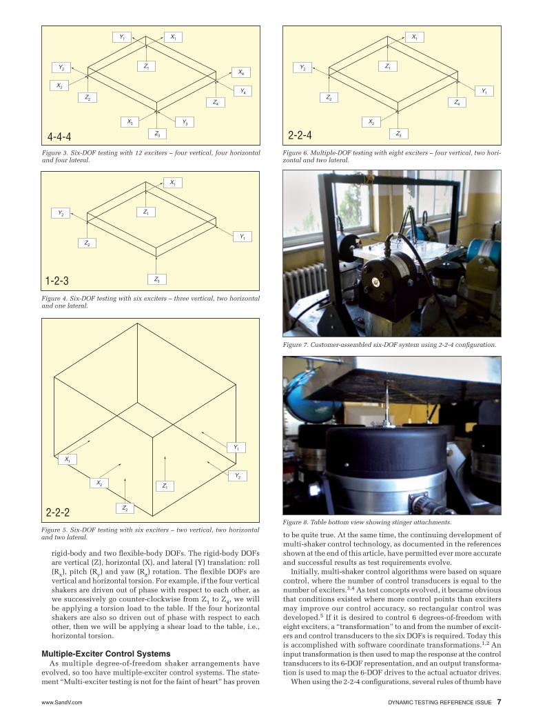
For Test A (Figure 9), no attempt was made to control phase or coherence between control locations for the off-diagonal terms of the spectral density matrix. Each of the eight exciters was driven with incoherent random signals and flat test profiles described from 100 Hz to 2,000 Hz.

With no attempt at phase correction, the test plate was free to respond in its own way. Figure 10 shows the resulting phase dif-ferences in the three principle axes. Note that the previous plots show the relative phase between control channels 1 to 8.5 In the interest of simplifying cable runs, the following controller channel assignments were made:

Figure 10a shows the relative phase for the Z controls, and Figure 10c shows the relative phase between the X and Y controls.

For Test B, the same 8 ¥ 8 square control arrangement was then used with full MIMO control of phase, magnitude and coherence. Phase was specified as zero and coherence as 0.97. The use of full MIMO control improved both the magnitude and phase parameters significantly, as seen in Figures 11 and 12.

From Figures 11 and 12, it is apparent that there are problems that are not being taken into account in addition to the inher-ent plate flexibility. One of these problems turned out to be the customer’s incorrect Y-axis directional definitions. The stingers also limited the levels that could be attained as a function of fre-quency. Note that in Figure 12, the adjacent corners are seen to be out of phase. But this is very likely influenced by the directional definitions.

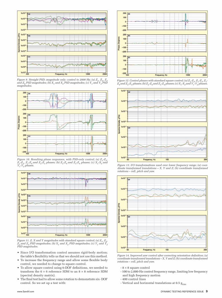
The next test, shown as D, is defined to use I/O transformations. Since the use of these transformations assumes rigid-plate response, the test was limited to 200 Hz, 100 control lines and 20% rotations. Figure 13b shows that roll and pitch were much better behaved than yaw. This turned out to be due to a bad definition of the Y-axis accelerometer mounting directions. When these orientation definitions were corrected, much improved yaw control was the result and is shown in Figure 14, test F.

At this point, we decided to increase the test level but also to introduce some tapering in the control spectrum shapes to limit the levels in the higher frequencies. The results are shown in Fig-ure 15, test G. They show better control uniformity and a higher upper frequency for control. The test results also confirm that the flexibility of the table is limiting the applicability of I/O transform control, since the table does not satisfy the needed rigid-body response assumption. So to progress, the control paradigm had to be changed. At this point, we felt that we knew enough about the structural and transducer setup to define a “final” control strategy. Also, it wouldn’t hurt to introduce a little “magic.”

So the following thought processes took place:• The customer wanted to test up to 2000 Hz. But so far, Tests A

and B were the only tests to 2000 Hz and they were relatively unsuccessful. A lot of this was attributed to the test levels, ref-erence PSD demands at the higher levels, and table flexibility.

• Table flexibility is the major culprit for this limitation, with limited force and small stinger connections also contributing. So this knowledge should be useable to increase the frequency range, which so far had been limited to about 500 Hz

• The customer also wanted to include significant rotational mo-tion in the final test.

Table 1. Reference grms level for MIMO random test from 40-2000 Hz.

Axis Acceleration, grms Equation X-Axis 0.5 X = (X1 + X2) / 2 Y-Axis 0.5 Y = (–Y1 – Y2) / 2 Z-Axis 3.0 Z = (Z1 + Z2 + Z3 + Z4) / 4 Roll 1.5 RX = (–Z1 – Z2 + Z3 + Z4) Pitch 1.5 RY = ( Z1 – Z2 – Z3 + Z4) Yaw 1.5 RZ = (X1 – Y1 – X2 + Y2)

(1)

X

Y

Z

R

R

R

x

y

z

Ï

Ì

ÔÔÔÔ

Ó

ÔÔÔÔ

¸

˝

ÔÔÔÔ

˛

ÔÔÔÔ

=

- -0 0 0 0 0 5 0 0 5 0

0 0 0 0 0 0 5 0 0 5

. .

. .

00 25 0 25 0 25 0 25 0 0 0 0

0 25 0 25 0 25 0 25 0 0 0 0

0 25 0 25 0 25 0

. . . .

. . . .

. . .

- -- - ..

. . . .

25 0 0 0 0

0 0 0 0 0 25 0 25 0 25 0 25

1

2

3

4

-

È

Î

ÍÍÍÍÍÍÍÍ

˘

˚

˙˙˙˙˙˙˙˙

Z

Z

Z

Z

X11

1

2

2

Y

X

Y

Ï

Ì

ÔÔÔÔÔ

Ó

ÔÔÔÔÔ

¸

˝

ÔÔÔÔÔ

˛

ÔÔÔÔÔ

Input Channel Number: 1 2 3 4 5 6 7 8Control Location: Z1 Z2 Z3 Z4 X1 Y1 X2 Y2

www.SandV.com DYNAMIC TESTING REFERENCE ISSUE 9

Figure 9. Straight PSD; magnitude only; control to 2000 Hz; (a) Z1, Z2, Z3 and Z4 PSD magnitudes; (b) X1 and X2 PSD magnitudes; (c) Y1 and Y2 PSD magnitudes.

Figure 10. Resulting phase responses, with PSD-only control; (a) Z1-Z2, Z1-Z3, Z1-Z4 and Z2-Z3 phases; (b) Z2-Z4 and Z3-Z4 phases; (c) X1-X2 and Y1-Y2 phases.

Figure 11. Z, X and Y magnitudes with standard square control; (a) Z1, Z2, Z3 and Z4 PSD magnitudes; (b) X1 and X2 PSD magnitudes; (c) Y1 and Y2 PSD magnitudes.

Figure 12. Control phases with standard square control; (a) Z1-Z2, Z1-Z3, Z1-Z4 and Z2-Z3 phases; (b) Z2-Z4 and Z3-Z4 phases; (c) X1-X2 and Y1-Y2 phases.

Figure 13. I/O transformations used over lower frequency range; (a) coor-dinate transformed translations – X, Y and Z; (b) coordinate transformed rotations – roll, pitch and yaw.

Figure 14. Improved yaw control after correcting orientation definition; (a) coordinate transformed translations – X, Y and Z; (b) coordinate transformed rotations – roll, pitch and yaw.

• Since I/O transformation control assumes rigid-body motion; the table’s flexibility tells us that we should not use this method.

• To increase the frequency range and allow some flexible body control, we needed to change to square control.

• To allow square control using 6-DOF definitions, we needed to transform the 6 ¥ 6 reference SDM to an 8 ¥ 8 reference SDM (spectral density matrix).

• The final test had to allow some rotation to demonstrate six- DOF control. So we set up a test with:

- 8 ¥ 8 square control- 100 to 2,000-Hz control frequency range, limiting low frequency and high frequency motion- 400 control lines- Vertical and horizontal translations at 0.5 grms

www.SandV.com10 SOUND & VIBRATION/OCTOBER 2013

Figure 15. Test G, 6 ¥ 8 I/O transforms with tapers on all control profiles; (a) coordinate transformed translations – X, Y and Z; (b) coordinate transformed rotations – roll, pitch and yaw.

Figure 16. Step 1 in calculating final square control matrix.

Figure 17. Step 2 in calculating final square control matrix.

Figure 18. Step 3 in calculating final square control matrix.

Figure 19. Test H, with Z, X and Y controls shown; (a) Z1, Z2, Z3 and Z4 PSD magnitudes; (b) X1 and X2 PSD magnitudes; (c) Y1 and Y2 PSD magnitudes.

- Roll, pitch and yaw rotations at 0.1 grmsSo for Test H, we needed to calculate the 8 ¥ 8 square SDM

control matrix from the 6-DOF reference matrix and the input transformation matrix. Figures 16 through 18 show the calculations performed to determine the needed SDM.6

Note that [INPUT] is the input transformation matrix defined in Eq. 1. The + superscript in Figure 18 denotes the pseudo inversion operation and not ordinary matrix inversion,7 while its T super-script denotes ordinary matrix transposition of [INPUT], which is a real rectangular matrix. The subscript terms, like 6 ¥ 8, denote the rank of the particular matrices following the respective operations of pseudo-inversion or matrix transposition. The final square SDM control matrix will therefore be of rank 8 ¥ 8.

Test H, as shown in Figure 19, has created a square control strat-egy to virtually eliminate the resulting plate resonances that were shown so prominently in Figure 11. At the same time, rotational motion was permitted to exist at relatively high levels. Test H was considered very successful by the customer and permitted the next step, using larger shakers, to move forward.

Conclusions• The use of I/O transformation control can lead to control prob-

lems at the frequencies that correspond to the (loaded) plate’s modal frequencies, since near those frequencies the plate does not move as a rigid body.

• Use the right-hand rule to determine the correct orientation of exciters and accelerometers to achieve good control with input/output transformations.

• Excellent control can be achieved using I/O transformations if it is limited to frequencies below which significant flexible-body motion begins to occur.

• Square control does not assume rigid-body motion and can be capable of controlling the plate’s motion much more effectively. However, care needs to be taken when the actuator configuration is over-actuated and the 6-DOF system’s platform is very stiff within the frequency range of interest.

• Square control is only appropriate if the plate and/or the actua-tor’s attachment to the plate is flexible. Alternatively, square or I/O transformation control can be used if there are enough actuators available with appropriate placement to counteract the plate’s modal reactions; i.e., its flexible body responses, which can effectively “unbend” the plate, if done properly.4

• Square control can achieve good control to 2 kHz in the flexible-body range. But square control needs strong, flexible attachments as the test levels increase.

• Rotational acceleration can be measured by taking the differences of accelerations, which are also divided by their moment arm, to obtain rotational motion in terms of radians/sec2 while using I/O transformations.

• Because of this, rotational acceleration may have a higher noise floor than linear acceleration measurements, which can make control more difficult. Higher sensitivity transducers can help mitigate this, or else the rotational levels to be controlled must be defined above the instrumentation’s noise floor.

• Sometimes, for structural reasons, it is better to allow for some

www.SandV.com DYNAMIC TESTING REFERENCE ISSUE 11

rotation so that actuators/fixtures/plate are not resisting rotation at the expense of controllability.

References1. Underwood, Marcos A., and Keller, Tony, “Applying Coordinate Trans-

formations to Multi-Degree-of-Freedom Shaker Control,” Proceedings of the 74th Shock & Vibration Symposium, San Diego, CA, October 2003.

2. Underwood, Marcos A., “Digital Control Systems for Vibration Testing Machines,” Shock and Vibration Handbook, 6th ed., Chapter 26, Edited by Piersol, A. G., and Paez, T. L., McGraw-Hill, New York, 2009.

3. Keller, Tony, and Underwood, Marcos A., “An Application of MIMO Techniques to Satellite Testing,” Presented at ESTECH 2000, Newport, RI, May 3, 2000.

4. Underwood, Marcos A., and Keller, Tony, “Recent System Developments for Multi-Actuator Vibration Control,” Sound & Vibration, October 2001.

5. Underwood, Marcos A., and Keller, Tony, “Rectangular Control of Multi-Shaker Systems; Theory and Some Practical Results,” Proceedings of the Institute of Environmental Sciences and Technology, ESTECH 2003, Phoenix, AZ, May 19, 2003.

6. Underwood, Marcos A., and Keller, Tony, “Understanding and Using the Spectral Density Matrix,” Proceedings of the 76th Shock & Vibration Symposium; Phoenix, AZ, October 2005. The author may be reached at: kellert@sd-star.com.

7. Underwood, Marcos A., “Applications of Computers to Shock and Vi-bration,” Shock and Vibration Handbook, 5th Ed., Chapter 27, Edited by Harris, C. M., and Piersol, A. G., McGraw-Hill, New York, 2001.

8. Hale, Michael, and Underwood, Marcos A., “MIMO Testing Methodolo-gies,” Proceedings of the 79th Shock & Vibration Symposium, Orlando, FL, October 26-30, 2008.

9. Ayres, Russell, Underwood, Marcos A., and Keller, Tony, “On Control-ling 6-DOF Electro-Dynamic Tables,” Presented at the 83rd Shock & Vibration Symposium, New Orleans, LA, November 4 -8, 2012.

10. Underwood, Marcos A., “A new Approach to System Identification, Using a Digitally Swept Multi-Exciter Sine Control System,” Acoustical Society of America 1989 Proceedings, Syracuse, NY.

11. Underwood, Marcos A., “The Adaptive Control of Multi-Exciters Using a Frequency-Domain Approach,” Ph.D. Dissertation, U.C.L.A. School of Engineering and Applied Sciences, 1993.

12. Underwood, Marcos A., “Adaptive Control Method for Multi-Exciter Sine Tests,” United States Patent, No. 5,299,459, April 1994.

13. Underwood, Marcos A., “Apparatus and Method for Adaptive Closed-Loop Control of Shock Testing System,” United States Patent, No. 5,517,426, May 1996.