Embed Size (px)
DESCRIPTION
Controller design by R.L. Typical setup:. C(s). G(s). Controller Design Goal: Select poles and zero of C(s) so that R.L. pass through desired region Select K corresponding to a good choice of dominant pole pair. Types of classical controllers. Proportional control - PowerPoint PPT Presentation
Citation preview
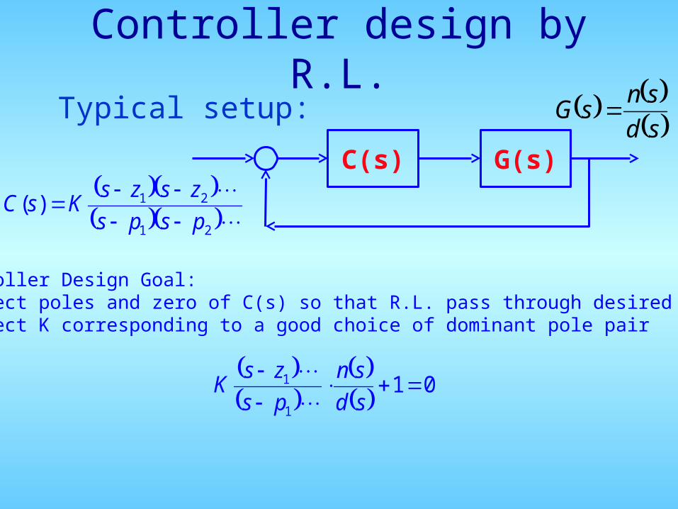
Controller design by R.L.Typical setup:
C(s) G(s)
01
1
1
sd
sn
ps
zsK
sdsn
sG
21
21)(psps
zszsKsC
Controller Design Goal: 1.Select poles and zero of C(s) so that R.L. pass through desired region2.Select K corresponding to a good choice of dominant pole pair
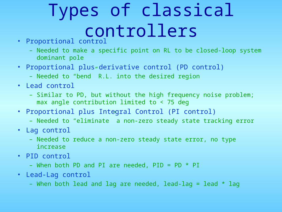
Types of classical controllers• Proportional control
– Needed to make a specific point on RL to be closed-loop system dominant pole
• Proportional plus derivative control (PD control)– Needed to “bend” R.L. into the desired region
• Lead control– Similar to PD, but without the high frequency noise problem; max angle
contribution limited to < 75 deg
• Proportional plus Integral Control (PI control)– Needed to “eliminate” a non-zero steady state tracking error
• Lag control– Needed to reduce a non-zero steady state error, no type increase
• PID control– When both PD and PI are needed, PID = PD * PI
• Lead-Lag control– When both lead and lag are needed, lead-lag = lead * lag
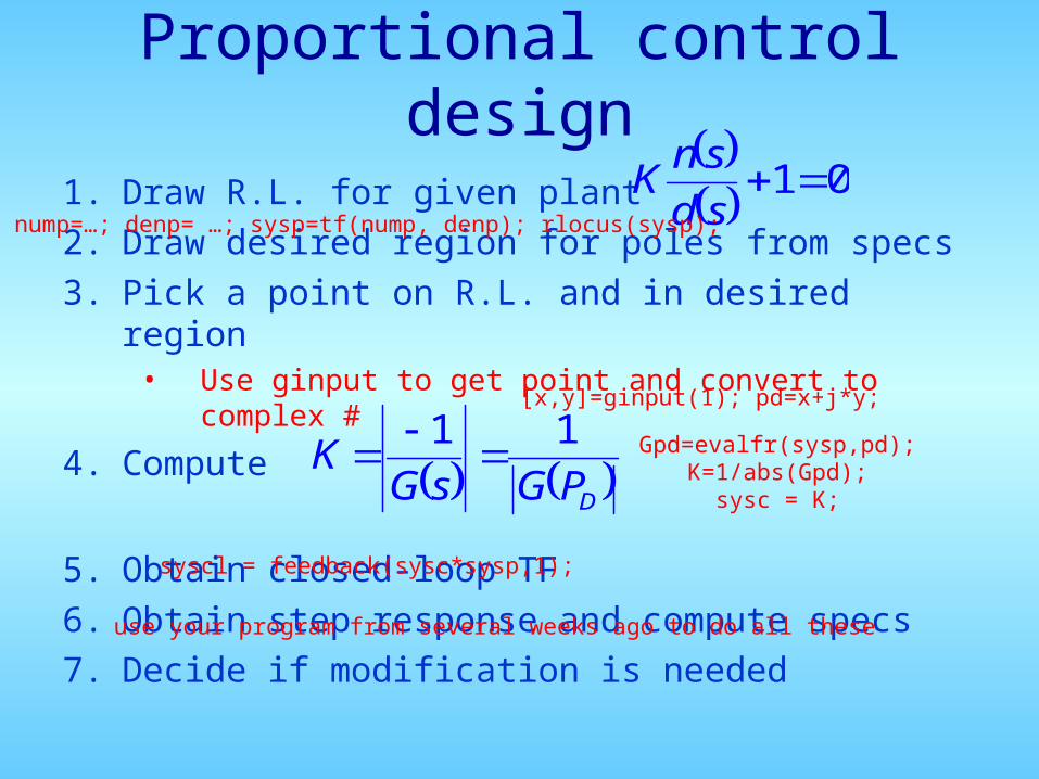
Proportional control design
1. Draw R.L. for given plant
2. Draw desired region for poles from specs
3. Pick a point on R.L. and in desired region• Use ginput to get point and convert to complex #
4. Compute
5. Obtain closed-loop TF
6. Obtain step response and compute specs
7. Decide if modification is needed
01sd
snK
DPGsGK
11
nump=…; denp= …; sysp=tf(nump, denp); rlocus(sysp);
use your program from several weeks ago to do all these
syscl = feedback(sysc*sysp,1);
Gpd=evalfr(sysp,pd);K=1/abs(Gpd);
sysc = K;
[x,y]=ginput(1); pd=x+j*y;
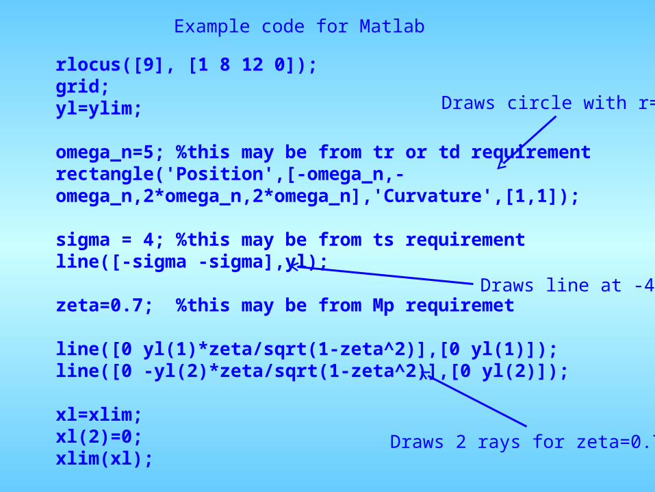
rlocus([9], [1 8 12 0]);grid;yl=ylim;
omega_n=5; %this may be from tr or td requirementrectangle('Position',[-omega_n,-omega_n,2*omega_n,2*omega_n],'Curvature',[1,1]);
sigma = 4; %this may be from ts requirementline([-sigma -sigma],yl);
zeta=0.7; %this may be from Mp requiremet
line([0 yl(1)*zeta/sqrt(1-zeta^2)],[0 yl(1)]);line([0 -yl(2)*zeta/sqrt(1-zeta^2)],[0 yl(2)]);
xl=xlim;xl(2)=0;xlim(xl);
Example code for Matlab
Draws circle with r=5
Draws line at -4
Draws 2 rays for zeta=0.7
-25 -20 -15 -10 -5 0 5 10-20
-15
-10
-5
0
5
10
15
20
0.98
0.140.30.440.580.72
0.84
0.92
0.98
510152025
0.140.30.440.580.72
0.84
0.92
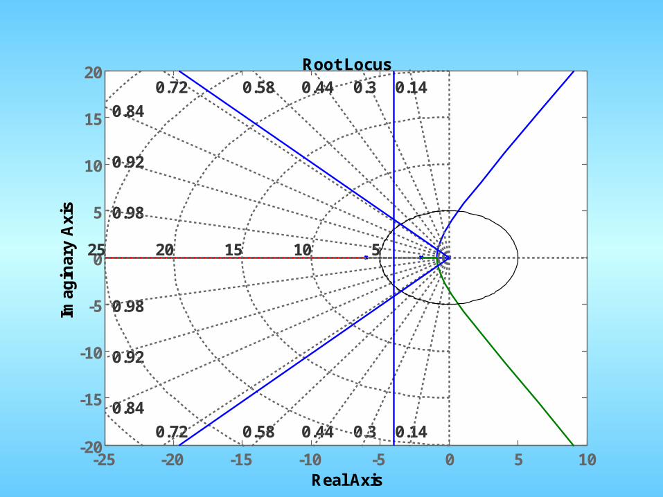
Root Locus
Real Axis
Imag
inar
y A
xis
-10 -8 -6 -4 -2 0
-4
-3
-2
-1
0
1
2
3
4
50.70.820.9
0.955
0.988
0.20.40.560.70.820.9
0.955
0.988
246810
0.20.40.56
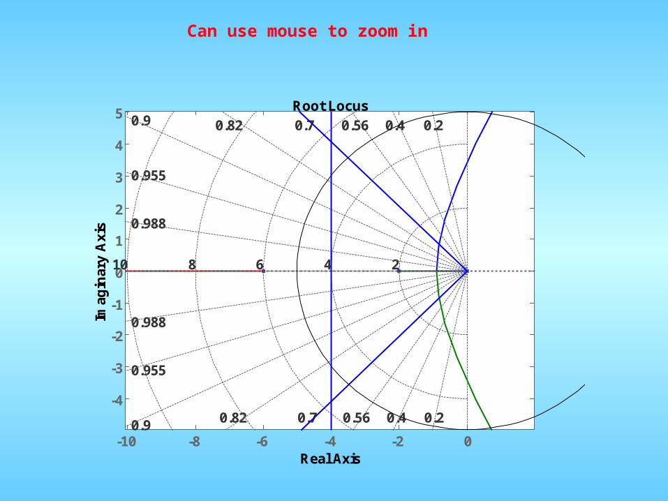
Root Locus
Real Axis
Imag
inar
y A
xis
Can use mouse to zoom in
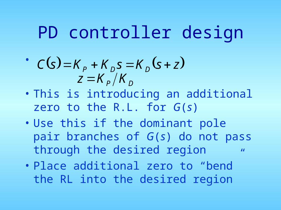
PD controller design
•
• This is introducing an additional zero to the R.L. for G(s)
• Use this if the dominant pole pair branches of G(s) do not pass through the desired region
• Place additional zero to “bend” the RL into the desired region
zsKsKKsC DDP DP KKz
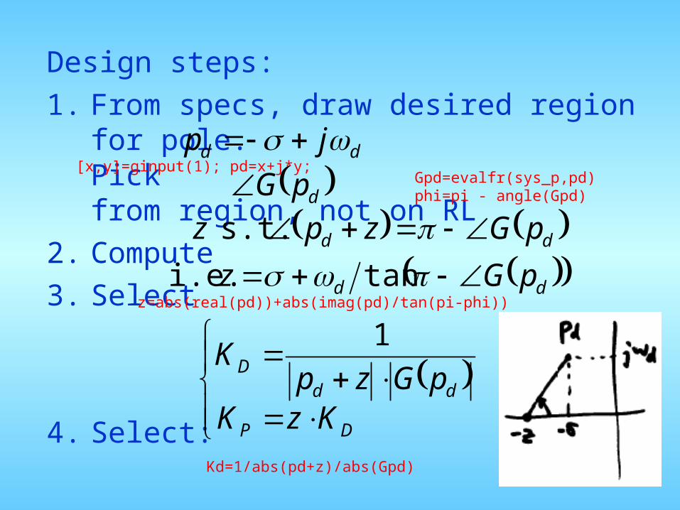
Design steps:
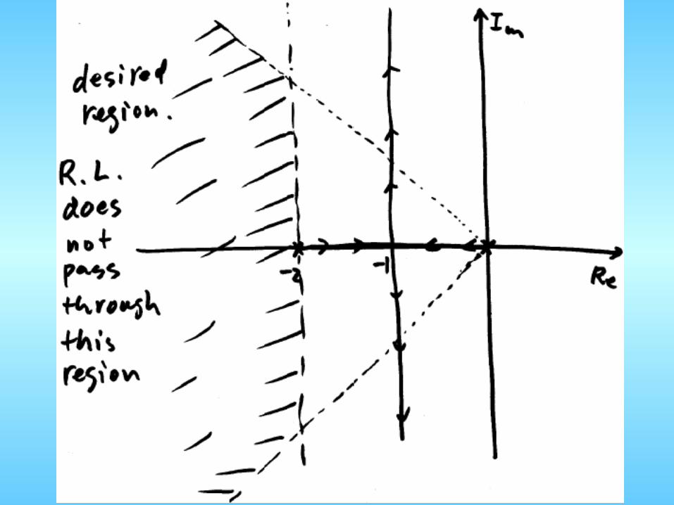
1. From specs, draw desired region for pole.Pick from region, not on RL
2. Compute
3. Select
4. Select:
dd jp dpG dd pGzpz s.t.
dd pGz tan i.e.
DP
ddD
KzKpGzp
K1
Gpd=evalfr(sys_p,pd)phi=pi - angle(Gpd)
z=abs(real(pd))+abs(imag(pd)/tan(pi-phi))
Kd=1/abs(pd+z)/abs(Gpd)
[x,y]=ginput(1); pd=x+j*y;
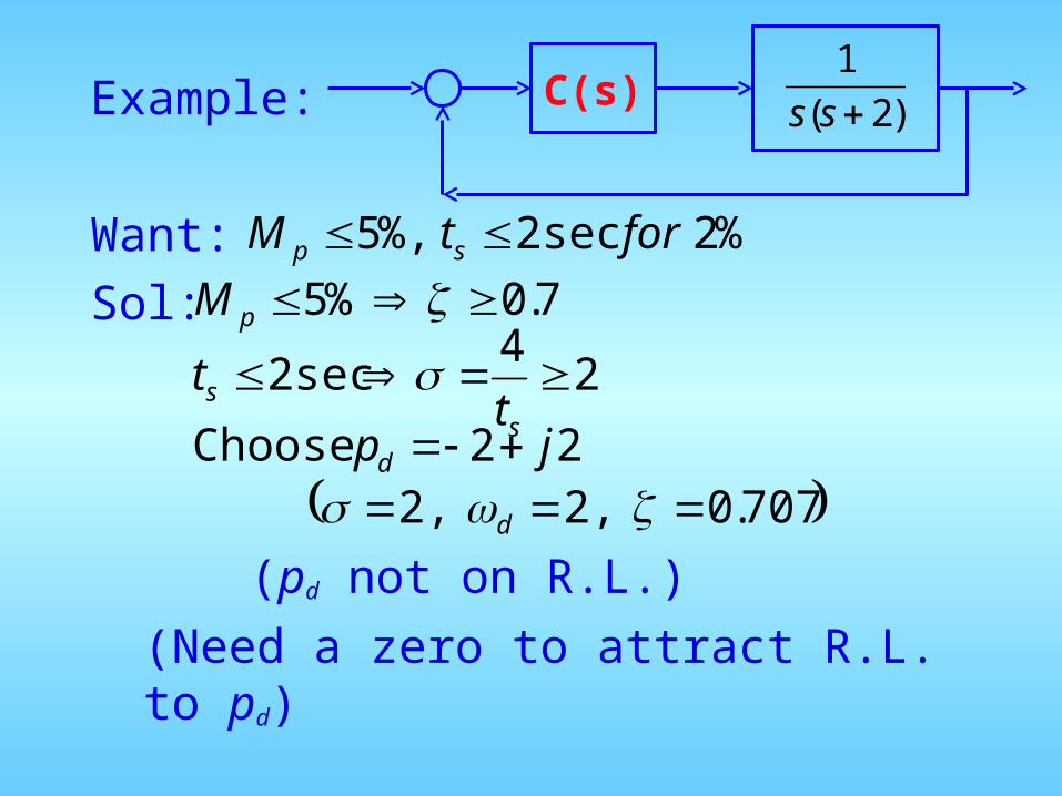
Example:
Want:Sol:
(pd not on R.L.)
(Need a zero to attract R.L. to pd)
%2sec2%,5 fortM sp 7.0%5 pM
24
sec2 s
s tt
22 Choose jpd 707.0,2,2 d
)2(
1
ssC(s)
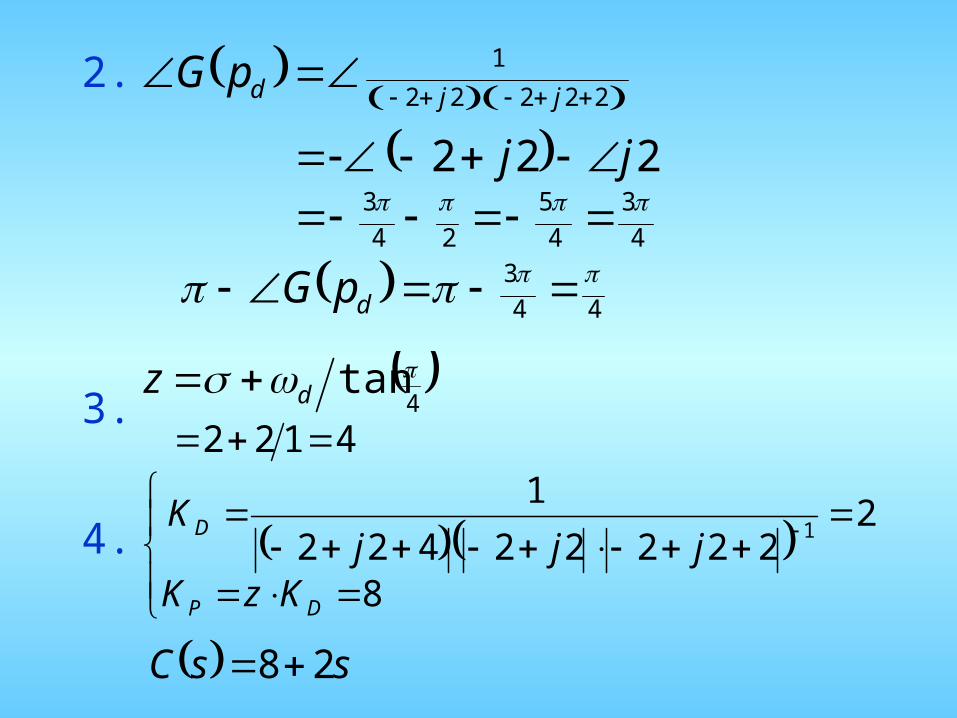
2.
3.
4.
4
tan dz
22222
1
jjdpG
222 jj
4
3
4
5
24
3
4122
8
222222422
11
DP
D
KzKjjj
K
ssC 28
44
3 dpG
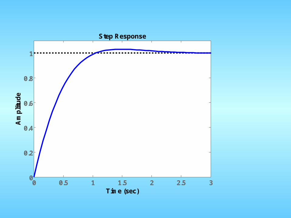
0 0.5 1 1.5 2 2.5 30
0.2
0.4
0.6
0.8
1
Step Response
Time (sec)
Am
plit
ud
e
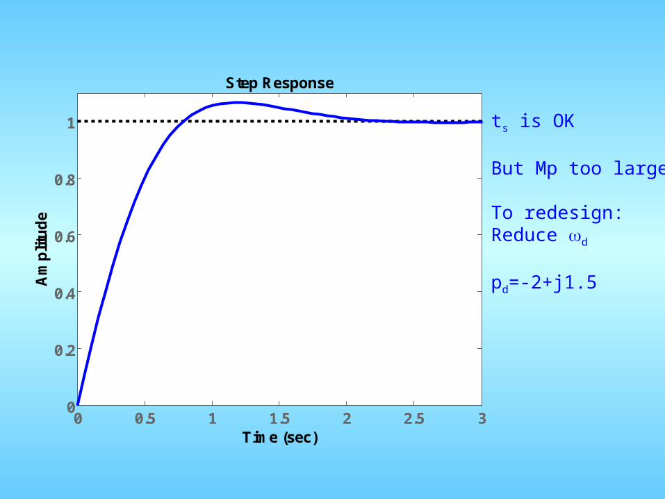
ts is OK
But Mp too large
To redesign:Reduce d
pd=-2+j1.5
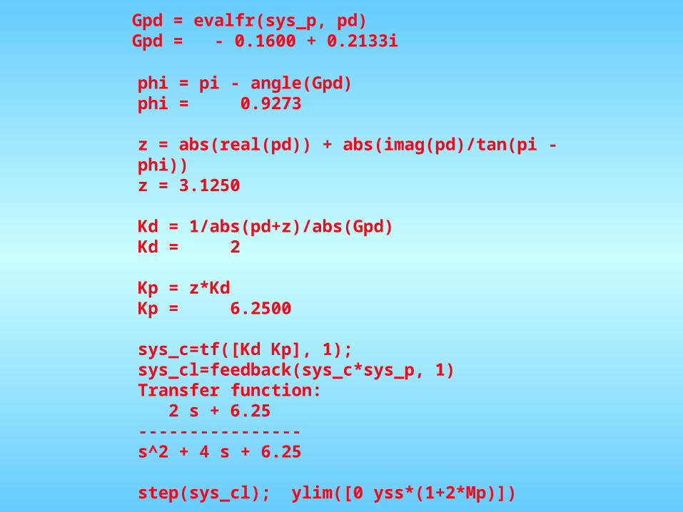
Gpd = evalfr(sys_p, pd)Gpd = - 0.1600 + 0.2133i
phi = pi - angle(Gpd)phi = 0.9273
z = abs(real(pd)) + abs(imag(pd)/tan(pi - phi))z = 3.1250
Kd = 1/abs(pd+z)/abs(Gpd)Kd = 2
Kp = z*KdKp = 6.2500
sys_c=tf([Kd Kp], 1);sys_cl=feedback(sys_c*sys_p, 1)Transfer function: 2 s + 6.25----------------s^2 + 4 s + 6.25
step(sys_cl); ylim([0 yss*(1+2*Mp)])
0 0.5 1 1.5 2 2.5 30
0.2
0.4
0.6
0.8
1
Step Response
Time (sec)
Am
plit
ud
e
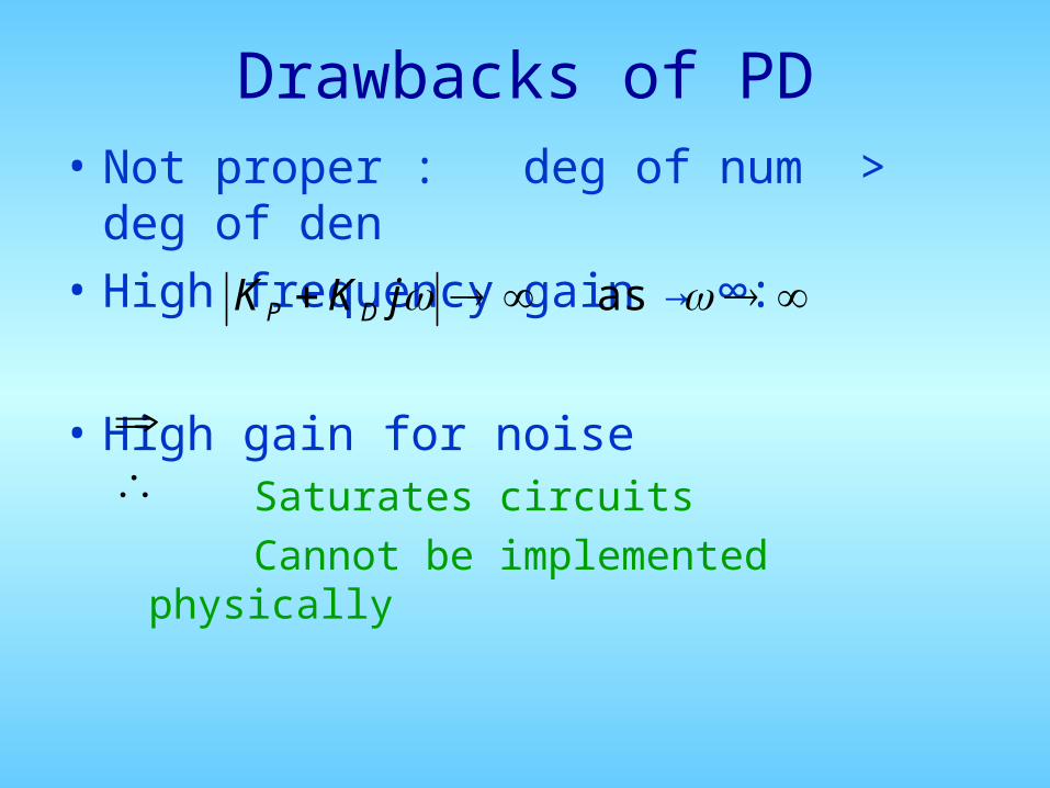
Drawbacks of PD• Not proper : deg of num > deg of den
• High frequency gain → ∞:
• High gain for noiseSaturates circuits
Cannot be implemented physically
as jKK DP
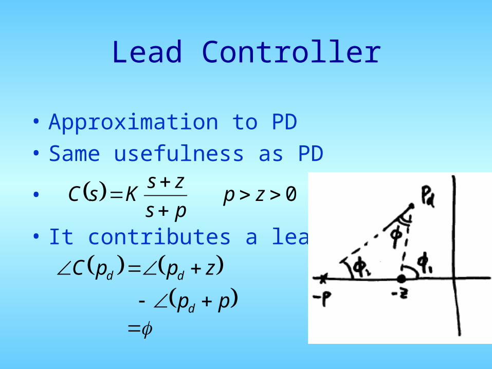
Lead Controller
• Approximation to PD
• Same usefulness as PD
•
• It contributes a lead angle:
0
zpps
zsKsC
zppC dd
ppd
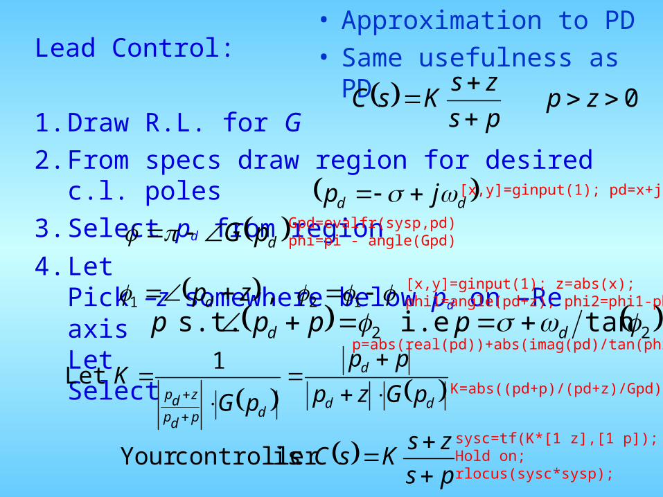
Lead Control:
1. Draw R.L. for G2. From specs draw region for desired c.l.
poles3. Select pd from region
4. LetPick –z somewhere below pd on –Re axisLetSelect
dd jp
dpG
121 ,zpd 2 s.t. ppp d 2tan i.e. dp
• Approximation to PD• Same usefulness as PD
0
zpps
zsKsC
dd
d
dpdp
zdp pGzp
pp
pGK
1Let
ps
zsKsC
:is controllerYour
[x,y]=ginput(1); z=abs(x);phi1=angle(pd+z); phi2=phi1-phi;
[x,y]=ginput(1); pd=x+j*y;
Gpd=evalfr(sysp,pd)phi=pi - angle(Gpd)
p=abs(real(pd))+abs(imag(pd)/tan(phi2));
K=abs((pd+p)/(pd+z)/Gpd);
sysc=tf(K*[1 z],[1 p]);Hold on;rlocus(sysc*sysp);
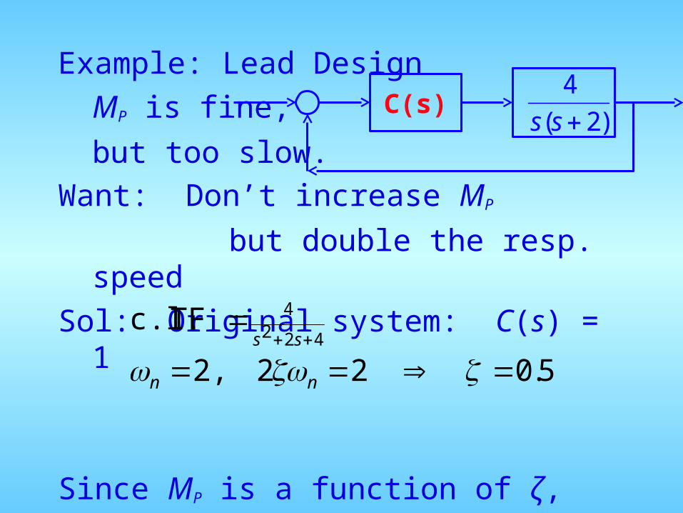
Example: Lead DesignMP is fine,
but too slow.Want: Don’t increase MP
but double the resp. speed
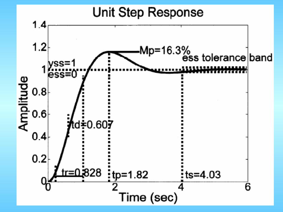
Sol: Original system: C(s) = 1
Since MP is a function of ζ, speed is proportional to ωn
5.022,2 nn
4224 TF c.l.
ss
C(s))2(
4
ss
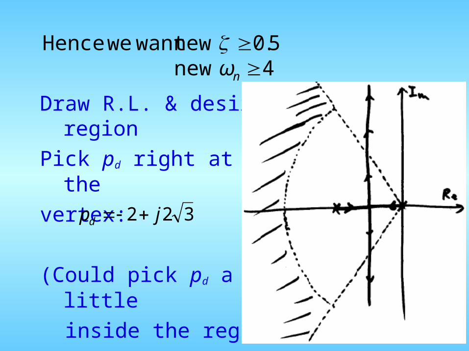
Draw R.L. & desiredregion
Pick pd right at the
vertex:
(Could pick pd a little
inside the region to allow “flex”)
5.0 new want weHence 4 new nω
322 jpd
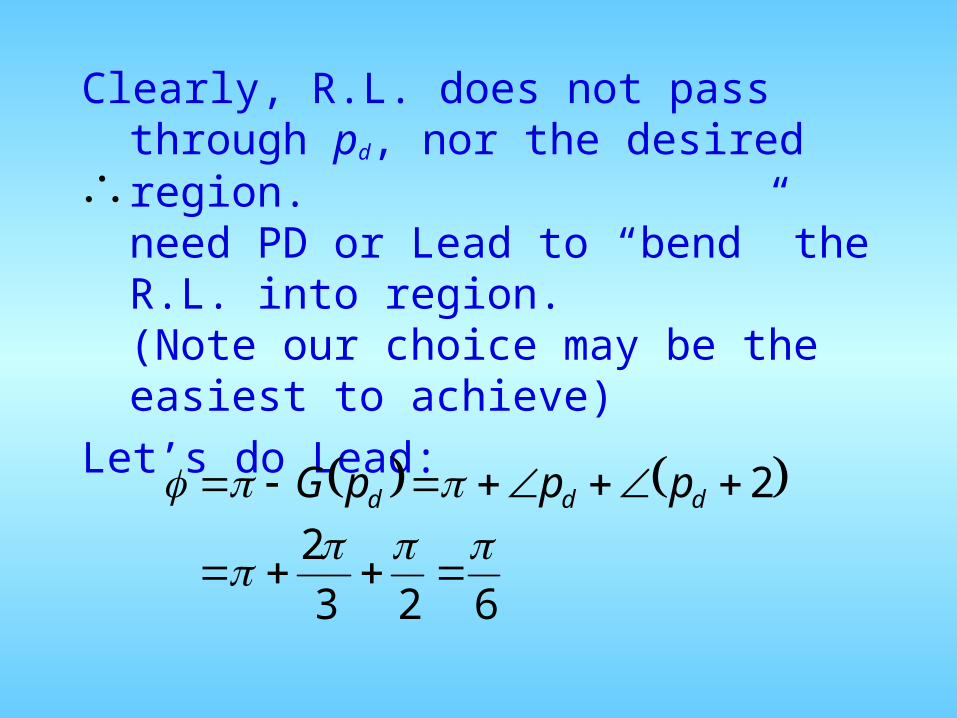
Clearly, R.L. does not pass through pd, nor the desired region.need PD or Lead to “bend” the R.L. into region.(Note our choice may be the easiest to achieve)
Let’s do Lead:
2 ddd pppG
623
2
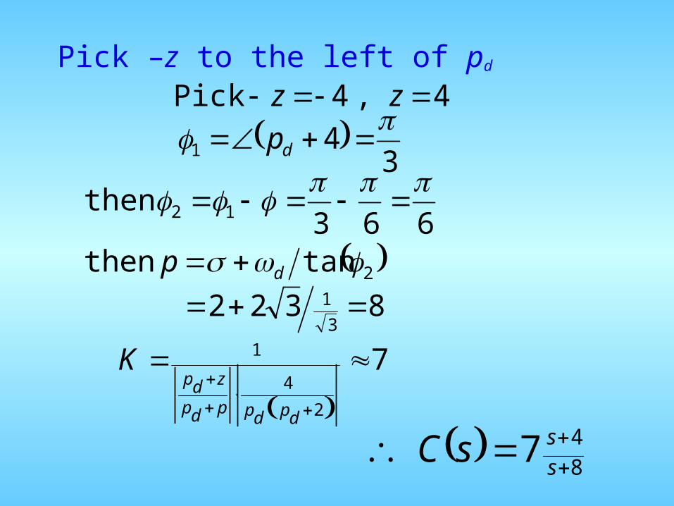
Pick –z to the left of pd
4,4Pick zz
3
41
dp
663then 12
2tanthen dp 8322
3
1
7
2
4
1
dpdppdp
zdpK
8
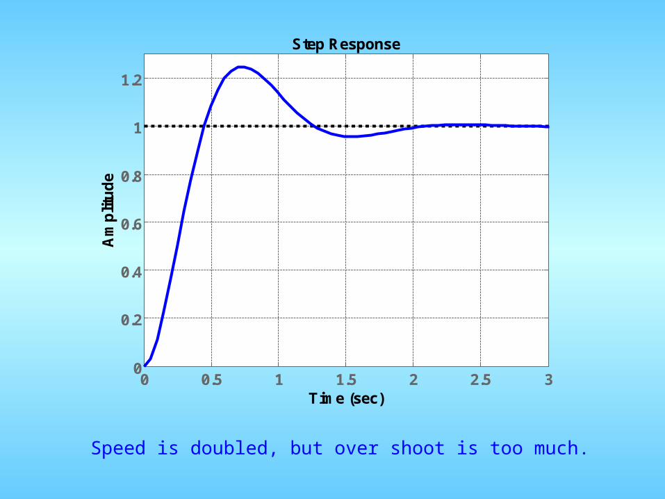
47 s
ssC
0 0.5 1 1.5 2 2.5 30
0.2
0.4
0.6
0.8
1
1.2
Step Response
Time (sec)
Am
plit
ud
e
Speed is doubled, but over shoot is too much.
0 0.5 1 1.5 2 2.5 30
0.2
0.4
0.6
0.8
1
1.2Step Response
Time (sec)
Am
plit
ud
e
8
47
s
ssC
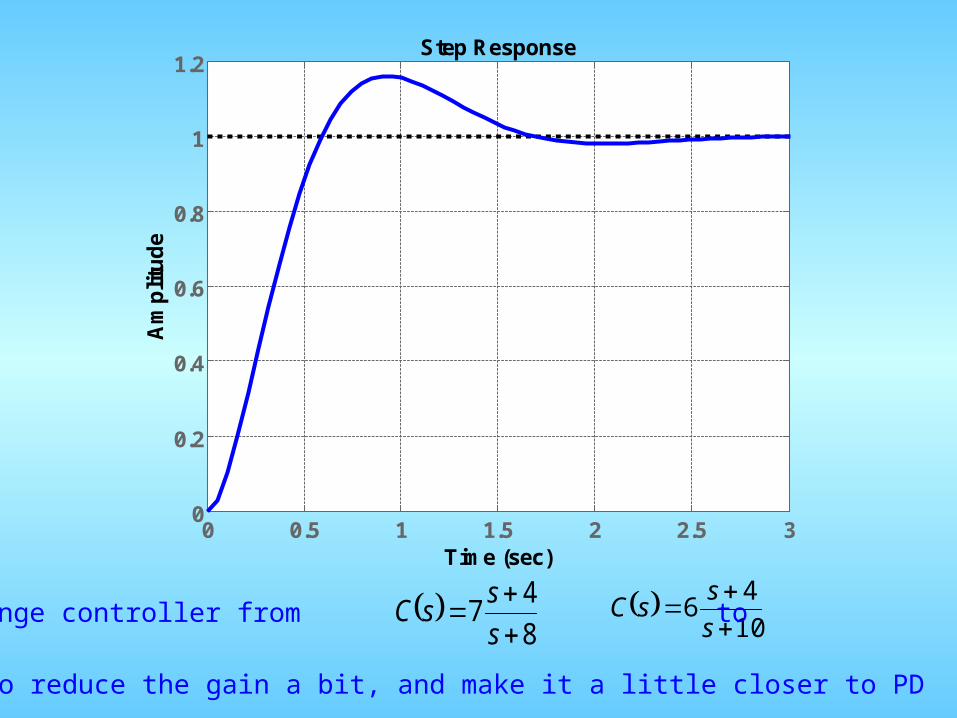
10
46
s
ssCChange controller from to
To reduce the gain a bit, and make it a little closer to PD
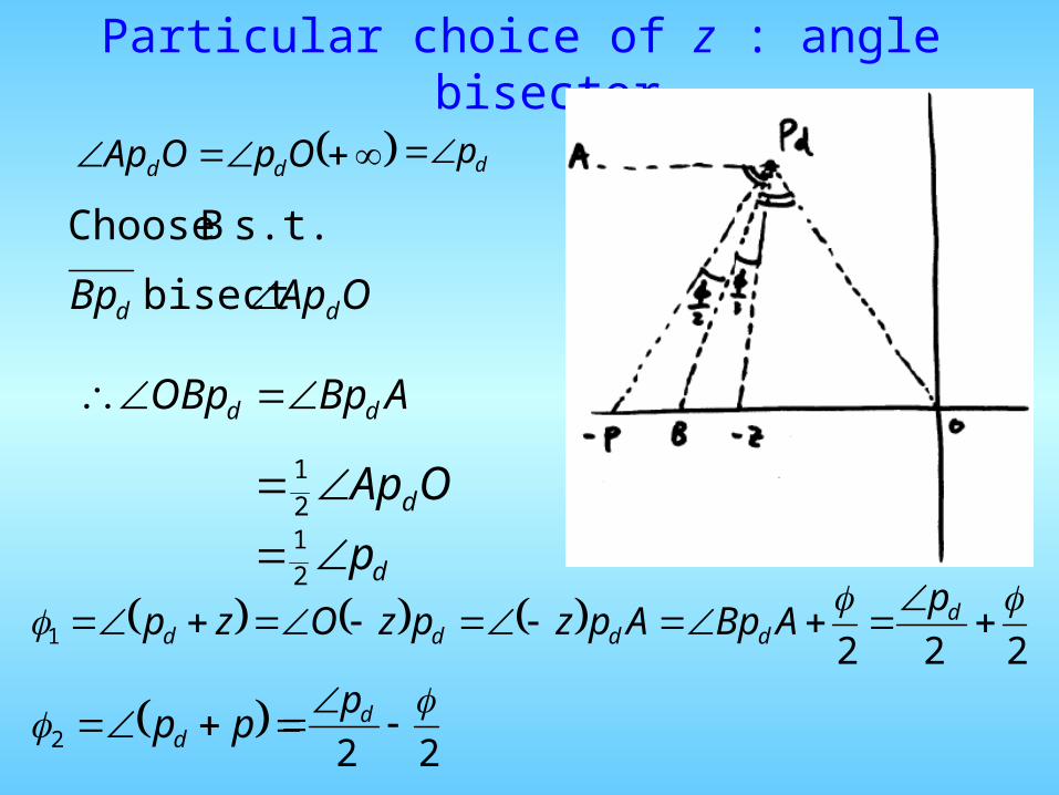
Particular choice of z : angle bisector
2221
ddddd
pABpApzpzOzp
ppd2
OpOAp dd dp
OApBp dd bisect
s.t. B Choose
ABpOBp dd
OApd2
1
dp2
1
22
dp
1tan dz 2tan dp
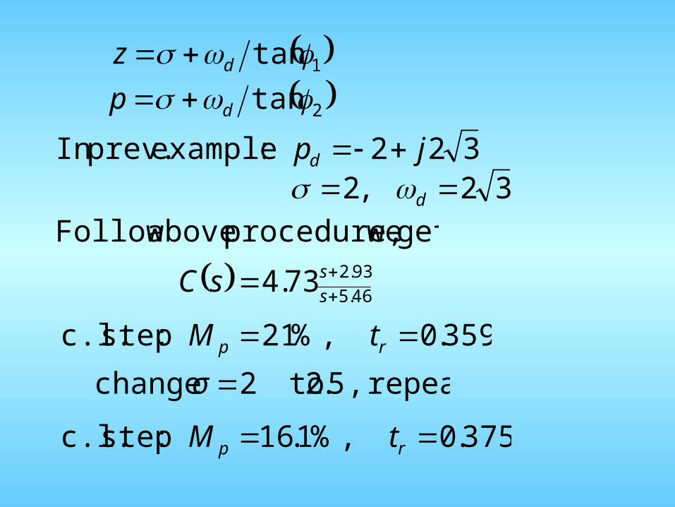
322 :example prev.In jpd 32,2 d
get weprocedure, above Follow
46.5
93.273.4 s
ssC
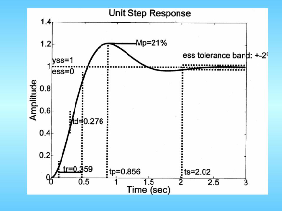
359.0,%21 :step c.l. rp tM
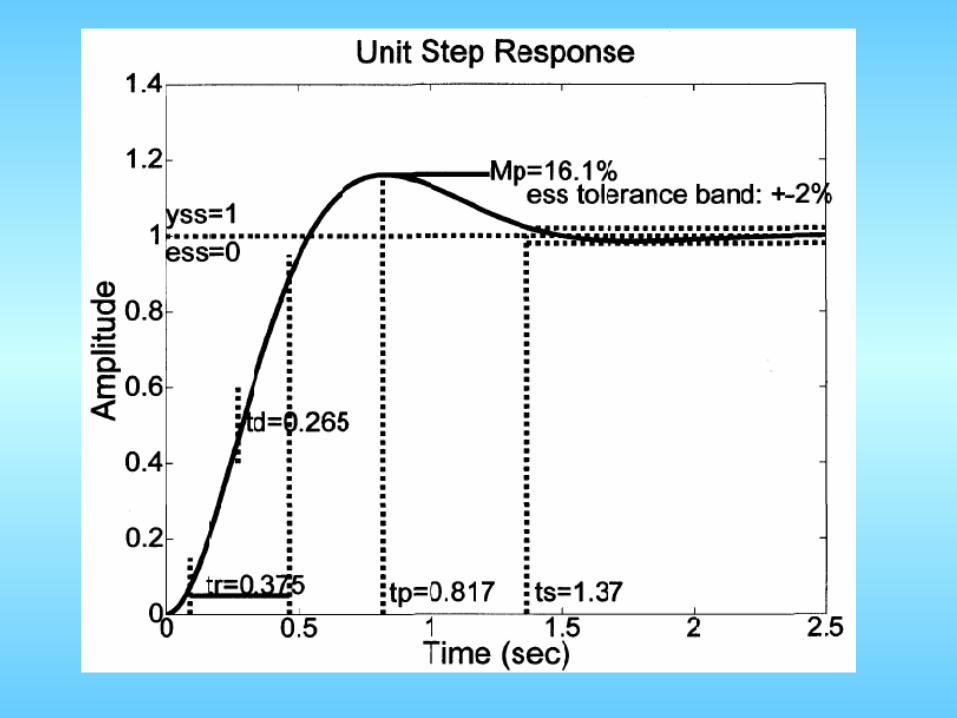
repeat. , 5.2 to2 change σ
375.0,%1.16 :step c.l. rp tM
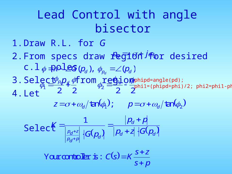
Lead Control with angle bisector1. Draw R.L. for G2. From specs draw region for desired c.l.
poles3. Select pd from region
4. Let
Select
dd jp
)(),( dpd ppGd
2222 21
dd pp
21 tan;tan dd pz
dd
d
dpdp
zdp pGzp
pp
pGK
1
ps
zsKsC
:is controllerYour
phipd=angle(pd);phi1=(phipd+phi)/2; phi2=phi1-phi;