Embed Size (px)
Citation preview

1 2 3 4 5 6 7 8 9 10 11 12 13 14 15 16 17 18 19 20 21 22 23 24 25 26 27 28 29 30 31 32 33 34 35 36 37 38 39 40 41 42 43 44 45 46 47 48 49 50 51 52 53 54 55 56 57 58 59 60 61 62 63 64 65
Control of ground-borne underground railway-inducedvibration from double-deck tunnel infrastructures by
means of dynamic vibration absorbers
Behshad Nooria,∗, Robert Arcosa,c, Arnau Clotb, Jordi Romeua
aAcoustical and Mechanical Engineering Laboratory (LEAM), Universitat Politecnica deCatalunya (UPC), Spain
bDepartment of Engineering, Cambridge University, United KingdomcSerra Hunter Fellow, Universitat Politecnica de Catalunya (UPC), Spain
Abstract
The aim of this study is to investigate the efficiency of Dynamic Vibration
Absorbers (DVAs) as a vibration abatement solution for railway-induced vibra-
tions in the framework of a double-deck circular railway tunnel infrastructure.
A previously developed semi-analytical model of the track-tunnel-ground sys-
tem is employed to calculate the energy flow resulting from a train pass-by.
A methodology for the coupling of a set of longitudinal distributions of DVAs
over a railway system is presented as a general approach, as well as its specific
application for the case of the double-deck tunnel model. In the basis of this
model, a Genetic Algorithm (GA) is used to obtain the optimal parameters of
the DVAs to minimize the vibration energy flow radiated upwards by the tunnel.
The parameters of the DVAs set to be optimized are the natural frequency, the
viscous damping and their positions. The results show that the DVAs would be
an effective countermeasure to address railway induced ground-borne vibration
as the total energy flow radiated upwards from the tunnel can be reduced by
an amount between 5.3 dB and 6.6 dB with optimized DVAs depending on the
type of the soil and the train speed.
Keywords: Railway-induced vibration, Dynamic vibration absorber,
∗Corresponding authorEmail address: [email protected] (Behshad Noori)

1 2 3 4 5 6 7 8 9 10 11 12 13 14 15 16 17 18 19 20 21 22 23 24 25 26 27 28 29 30 31 32 33 34 35 36 37 38 39 40 41 42 43 44 45 46 47 48 49 50 51 52 53 54 55 56 57 58 59 60 61 62 63 64 65
Double-deck tunnel, Vibration energy flow
1. Introduction
The passage of trains in underground tunnels is one of the major sources
of ground-borne vibrations. These vibrations propagate through the soil and
structures of nearby buildings, resulting in undesired vibration and re-radiated
noise inside the buildings. They may cause discomfort to the building residents,
affect the operation of sensitive equipment and damage historical edifices with
structural weakness. In recent years, innovative tunnel structure designs, like
double-deck tunnels, have been constructed in several cities worldwide while few
studies have been reported on appropriate measures to mitigate ground-borne
vibration for these new designs.
Several countermeasures have been proposed to address the problem of
ground-borne vibration induced by railways. These solutions can be categorized
according to the location where they are applied: i) the source [1, 2]; ii) the re-
ceiver [3, 4] and iii) the propagation path [5, 6]. Accurate prediction models
should be used to assess the efficiency of these mitigation measures. Numerical,
hybrid models and semi-analytical models can provide the desired level of accu-
racy. In the framework of numerical models, two-and-a-half-dimensional (2.5D)
approaches based on Finite Element-Boundary Element Methods (FEM-BEM)
[7–9], and the Method of Fundamental Solutions (MFS) coupled with FEM
[10] are the common approaches. For specific sites, hybrid models [11, 12] can
provide an increment on the accuracy with respect to conventional numerical ap-
proaches. Regarding semi-analytical models, probably the most well-established
models for underground railway traffic is the Pipe-in-Pipe (PiP) model [13, 14].
An extension of the PiP model was also presented by Hussein et al. [15] to
calculate the vibrations from a tunnel embedded in a layered half-space, in
which 2.5D Green’s functions of a half-space can be evaluated using 3D stiffness
matrices cast in cylindrical coordinates [16] or Cartesian coordinates [17].
A well-established system that has been widely used to control the vibration
2

1 2 3 4 5 6 7 8 9 10 11 12 13 14 15 16 17 18 19 20 21 22 23 24 25 26 27 28 29 30 31 32 33 34 35 36 37 38 39 40 41 42 43 44 45 46 47 48 49 50 51 52 53 54 55 56 57 58 59 60 61 62 63 64 65
of mechanical, civil and aerospace structures is the Dynamic Vibration Ab-
sorber (DVA), also known as Tuned Mass Damper (TMD). In the last century,
the application of DVAs as passive, active and semi-active countermeasures to
attenuate undesirable vibration has been studied extensively [18, 19]. Some of
the prominent applications of DVAs around the globe are the ones in Taipei
World Financial Center (also known as Taipei 101) [20], Millennium Bridge [21]
and Doha Sport City Tower [22]. DVA is usually modeled as a single-degree-
of-freedom (SDOF) and it works as a secondary oscillatory system applied on
a primary system where the vibration needs to be controlled. The concept of
a DVA was outlined by Watts in 1883 [23]. However, the practical design of
a DVA, as a spring-supported mass, was proposed by Frahm in 1911 [24]. A
damping element was later introduced to DVAs to widen the controlled fre-
quency range [25]. DVAs can be used to attenuate the vibration at a specific
frequency or over a particular range of frequencies. In the former case, the
natural frequency of the DVA should be tuned to the specific frequency, and
the damping should be chosen as low as possible [26]. In the latter case, an
optimization criterion is required as the effectiveness of a DVA depends on its
parameters.
Several types of optimization procedures with analytical or numerical ap-
proaches can be considered to determine the optimal value of DVA parameters
[18, 27–29]. In most of the analytical optimization procedures that are em-
ployed to find the optimal value of DVA parameters, the structure on which
the DVAs are applied (the host structure) is modeled as a SDOF system [28].
In these methodologies, the parameters of this SDOF model are obtained from
the dominant mode of the host structure response. However, there are other
optimization procedures that dont require a prior determination of which mode
must be controlled. Among those, Genetic Algorithms (GAs) have been widely
used for tuning DVA parameters in order to optimally reduce the vibration in
specific locations of the system or in a global point of view. Some of the studies
that apply GA for this purpose are [28, 30–33].
Recently, DVAs have been used to address some issues in the railway-induced
3

1 2 3 4 5 6 7 8 9 10 11 12 13 14 15 16 17 18 19 20 21 22 23 24 25 26 27 28 29 30 31 32 33 34 35 36 37 38 39 40 41 42 43 44 45 46 47 48 49 50 51 52 53 54 55 56 57 58 59 60 61 62 63 64 65
vibration field. A study on the effectiveness of DVAs in suppressing the low-
frequency vibrations of floating slab track with discontinuous slabs was con-
ducted by Zhu et al. [34] using a FEM model. They used two DVAs to mini-
mize first- and second-mode vibrations of a slab which was treated as a SDOF
system with the parameters of the selected mode, and the optimal parameters
of DVAs were found using fixed-point theory [35]. Reducing the vibration of
car-bodies of a low-floor train at a certain frequency by means of a DVA was
investigated by Wang et al. [36], in which the DVA was found to be an effective
countermeasure for excessive vertical vibration of car-bodies. DVAs have been
also found to be effective in reducing the noise radiated by a rail. Thompson
et al. [37] designed DVAs of steel masses and elastomeric material with a high
damping loss factor, placed at both sides of the rail. The system of absorbers
results in a reduction of radiated noise by about 5–6 dB. These DVAs were re-
ported to be effective in slowing the growth of rail corrugation if they can fully
suppress the pinnedpinned resonance [38]. Ho et al. developed multiple DVAs
each consisting of a mass sandwiched between resilient materials [39]. This mul-
tiple mass–spring system has been put into practice and the system is found to
be effective not only in attenuating rail vibration and the tunnel noise level [39]
but also in slowing the growth of rail corrugation [40].
Double-deck circular tunnels are an innovative design underground transport
infrastructures in which the tunnel is divided into two sections by an interior
floor. The definition and design methodology of specific mitigation measures
for ground-borne vibrations have not been studied adequately yet for this type
of tunnel. The modification of the stiffness/damping values of the rail pads [41]
and implementation of an elastomeric mat between the interior floor and the
tunnel structure [41, 42] are two mitigation measures studied by Clot et al.,
using a 2.5D semi-analytical model of a double-deck tunnel [43]. It was found
that implementing a soft elastomeric mat reduces the soil vibration considerably.
The potential of DVA as a vibration countermeasure for underground railway-
induced ground-borne vibration problems can be investigated for the full- and
half-space cases as a model of the soil. The full-space model is used to generally
4

1 2 3 4 5 6 7 8 9 10 11 12 13 14 15 16 17 18 19 20 21 22 23 24 25 26 27 28 29 30 31 32 33 34 35 36 37 38 39 40 41 42 43 44 45 46 47 48 49 50 51 52 53 54 55 56 57 58 59 60 61 62 63 64 65
evaluate the effect of DVAs by controlling the vibration energy radiated up-
wards by the tunnel structure. This model would be useful to address vibration
problems of long railway sections, where different buildings and tunnel depths
are involved, without of requiring a complicated model in which the particular
foundation/geometry of nearby buildings need to be taken into account. On the
other hand, the half-space model would be more convenient to study the vibra-
tion mitigation for specific buildings using a model in which the soil-building
interaction is also considered.
In this paper, the application of DVAs on the upper section of a double-deck
tunnel to minimize the energy flow radiated upwards resulting from the train
pass-by over this section is studied through the full-space approach. The vehicle-
track-tunnel-soil model is employed, in which the track-tunnel-soil model is the
one developed by Clot et al. [43] and the train-track model is an extension
of the model presented in [44] by considering two 2D vehicle models over the
two rails. The rest of the paper is organized as follows: In Section 2, the
vehicle-track-tunnel-soil model is described; Section 3 is dedicated to details
regarding the coupling of DVAs to an underground railway infrastructure model.
The optimization method to determine the optimal parameters of the DVAs to
minimize energy flow radiated upwards for the case of an underground double-
deck tunnel railway infrastructure is presented in Section 4. The efficiency of a
set of DVAs as a vibration countermeasure applied to the specific case studies
to minimize the radiated energy flow is discussed in Section 5. Finally, results
obtained from this study are summed up in Section 6.
2. Modeling of the vehicle-track-tunnel-soil system
This section starts by recapitulating the considered 2.5D semi-analytical
model of a double-deck tunnel embedded in a full-space [43]. This model pro-
vides the 2.5D Green’s functions of the system due to loads applied on the rails
and on the interior floor, which are required to couple the train and the DVAs
to the system and to compute the train pass-by response. Then, the considered
5

1 2 3 4 5 6 7 8 9 10 11 12 13 14 15 16 17 18 19 20 21 22 23 24 25 26 27 28 29 30 31 32 33 34 35 36 37 38 39 40 41 42 43 44 45 46 47 48 49 50 51 52 53 54 55 56 57 58 59 60 61 62 63 64 65
train-track interaction model is described, followed by an explanation of how
this model is employed to determine the response of the system due to a train
pass-by.
2.1. Track-tunnel-soil model
A scheme of the model considered for the track-tunnel-soil system is shown
in Fig. 1. The track consists of two rails connected to the interior floor of
the double-deck tunnel structure by means of direct fixation fasteners, and the
tunnel is assumed to be embedded in a homogeneous full-space. The system
is considered to be invariant in the longitudinal direction, i.e., the direction in
which the train circulates.
Rails
Interior Floor
Tunnel
Tunnel
kf ,cf f ,cf
Interior Floor
rt
k
Soil
kf ,cf
Fig. 1: A scheme of a double-deck tunnel and its subsystems embedded in a full-space.
The rails are modeled as Euler-Bernoulli beams of infinite length separated
by a specific distance. The direct fixation fastener is represented by a contin-
uous mass-less distribution of springs, with a stiffness per unit length kf , and
dashpots, with a viscous damping per meter cf . The interior floor is modeled
as a homogeneous isotropic thin strip plate with a rectangular cross-section.
The tunnel and soil subsystems are described using the PiP model, developed
by Forrest and Hunt [13], which assumes that they can be represented as an
infinite thin cylindrical shell and as an infinite homogeneous elastic medium,
6

1 2 3 4 5 6 7 8 9 10 11 12 13 14 15 16 17 18 19 20 21 22 23 24 25 26 27 28 29 30 31 32 33 34 35 36 37 38 39 40 41 42 43 44 45 46 47 48 49 50 51 52 53 54 55 56 57 58 59 60 61 62 63 64 65
respectively.
2.2. Vehicle-track coupling
There are two excitation mechanisms that mostly contribute to the vibra-
tion induced by railway traffic: i) the quasi-static excitation ii) the dynamic
excitation. The former is induced by the static component of the moving loads
applied by the train to the track and is of great importance for high-speed trains.
The latter can be attributed to various mechanisms [45], mainly the wheel/rail
unevenness and the longitudinal variability of the track’s mechanical parame-
ters. Since the present investigation is done in the context of urban railway
infrastructure, the vertical dynamic excitation caused by the rail unevenness is
considered as the only excitation source. It is assumed that the unevenness of
the rails is uncorrelated between them [46].
Consider a moving frame of reference associated to a train motion. Due to
the Doppler effect, the frequency components of the time signals seen from the
perspective of this moving frame of reference (ω) are different from the ones
related to a fixed frame of reference (ω) [44]. All the derivation presented in
this section is based on the moving coordinate system, thus, all the variables
represented in the frequency domain are associated to the frequency ω, except
when it is specifically mentioned otherwise. Capital letters notation is used to
denote variable in the frequency domain.
The vertical displacements of the two rails in the frequency domain due to
the wheel/rail contact forces can be represented byZw/rr1
Zw/rr2
=
Hw/rr1r1 H
w/rr1r2
Hw/rr2r1 H
w/rr2r2
F
w/rr1
Fw/rr2
, (1)
where Zw/rr1 and Z
w/rr2 are the vertical displacements of the left and right rails,
respectively, at all the vehicle axle positions, Hw/rr1r1 and H
w/rr2r2 are the direct
receptance matrices of the left and right rails, respectively, at all the axles
positions, Hw/rr2r1 = H
w/rr1r2 is the cross receptance matrix between the left and
7

1 2 3 4 5 6 7 8 9 10 11 12 13 14 15 16 17 18 19 20 21 22 23 24 25 26 27 28 29 30 31 32 33 34 35 36 37 38 39 40 41 42 43 44 45 46 47 48 49 50 51 52 53 54 55 56 57 58 59 60 61 62 63 64 65
right rails at all axle positions, Fw/rr1 and F
w/rr2 are the vectors of wheel/rail
interaction forces associated to the left and right rails, respectively; and the
response of the two half vehicles can be written byZw/rv1
Zw/rv2
= −
Hw/rv1 0
0 Hw/rv2
F
w/rr1
Fw/rr2
, (2)
where Zw/rv1 and Z
w/rv2 are the vertical displacements of vehicle wheels in contact
with the left and right rails, respectively, and Hw/rv1 and H
w/rv2 are the receptances
of each half vehicle at all the vehicle axle positions. Eqs. (1) and (2) can easily
be compacted to
Zw/rr = Hw/rr Fw/r, Zw/rv = −Hw/r
v Fw/r. (3)
Consider now that the 2.5D Green’s functions associated to the studied
railway infrastructure system are obtained on the basis of a double Fourier
transform (FT) defined by
G(kx, ω) =
∫ +∞
−∞
∫ +∞
−∞g(x, t)ei(kxx−ωt)dxdt. (4)
where x, t, kx and ω represent the longitudinal coordinate, the time, the
wavenumber associated to the longitudinal coordinate and the frequency seen
from a fixed frame of reference, respectively. Combined bar and capital letters
notation is used to denote variables in the wavenumber-frequency domain on a
fixed frame of reference. Taking this into account, the elements of the receptance
matrices required to construct Hw/rr can be computed by
Hw/rrirj ,nm =
1
2π
∫ +∞
−∞Hrirje−ikx(xn−xm)dkx, (5)
where Hw/rrirj ,nm is the (n,m) element of the matrix H
w/rrirj , xn and xm are the
longitudinal coordinates of the n-th and m-th axles, respectively, seen from the
point of view of the moving frame of reference, and Hrirj is the 2.5D Green’s
8

1 2 3 4 5 6 7 8 9 10 11 12 13 14 15 16 17 18 19 20 21 22 23 24 25 26 27 28 29 30 31 32 33 34 35 36 37 38 39 40 41 42 43 44 45 46 47 48 49 50 51 52 53 54 55 56 57 58 59 60 61 62 63 64 65
function of the system defined in the (kx, ω) domain that relates the verti-
cal motions of the rails ri and rj . A 2.5D Green’s function defined in the
(kx, ω) domain can be obtained from the one defined in the (kx, ω) domain by
H(kx, ω) = H(kx, ω+kxvt), being vt the speed of the train. Note that combined
∼ and capital letters notation is used to denote variables in the wavenumber-
frequency domain on a moving frame of reference. The vehicle receptance matrix
is obtained by means of the dynamic model of the vehicle, which in this inves-
tigation is considered to be the two-dimensional (2D) multi-degree-of-freedom
rigid body model presented by Lei and Noda [47]. A 3D model of each car
consists of two uncoupled 2D models separately applied on each rail. A global
train is modeled as a set of Nc identical cars.
Assuming a linearized Hertz contact, the wheel/rail interaction forces can
be obtained in the frequency domain by using
Fw/r = kH
(Zw/rv − Zw/rr + Er
), (6)
where kH is the stiffness of the linearized Hertzian spring, considered to be the
same in all the wheel/rail contacts, and Er is the vector of complex amplitudes
of rails unevenness at all the wheel/rail contacts. Combining Eq. (6) with Eq.
(3) one can obtain a transfer function in the frequency domain between the
unevenness of the rails and the dynamic wheel/rail interaction forces, which
may be written as
Fw/r =(Hw/rv + Hw/r
r + k−1H I)−1
Er, (7)
where I is the identity matrix.
Once the wheel/rail interaction forces are computed, the response at an
arbitrary position l of the railway infrastructure system due to the passage of
the train can be found using the expression
ul(x, t) =
2∑i=1
1
2π
∫ +∞
−∞
Na∑n=1
[1
2π
∫ +∞
−∞HlriF
w/rri,n e−ikx(x−xn)dkx
]eiωtdω, (8)
9

1 2 3 4 5 6 7 8 9 10 11 12 13 14 15 16 17 18 19 20 21 22 23 24 25 26 27 28 29 30 31 32 33 34 35 36 37 38 39 40 41 42 43 44 45 46 47 48 49 50 51 52 53 54 55 56 57 58 59 60 61 62 63 64 65
where ul(x, t) is the displacement response at l position of the railway infras-
tructure system, Hlri is the 2.5D Green’s function in the wavenumber-frequency
domain that relates the displacement response at that arbitrary position l with
a force applied in the i-th rail, x is the longitudinal coordinate associated to the
moving frame of reference, Na is the number of axles of the train and Fw/rri,n is
the wheel/rail interaction force associated to the i-th rail and the n-th axle. An
equivalent expression for the soil tractions can be obtained by simply replacing
the displacement Green’s functions with those for the tractions in Eq. (8). The
expression of the soil vibration velocity can be written similarly to Eq. (8) as
vl(x, t) =
2∑i=1
1
2π
∫ +∞
−∞
Na∑n=1
[1
2π
∫ +∞
−∞i(ω + kxvt)HlriF
w/rri,n e−ikx(x−xn)dkx
]eiωtdω,
(9)
3. Application of DVAs on an underground railway system
This section starts with the explanation of a methodology which can be used
to couple a set of DVAs to any subsystem of a railway infrastructure. Then,
the application of this methodology for the case of the double-deck tunnel is
explained.
DVAs can be applied on different subsystems of a railway infrastructure, such
as the tunnel or the track. For example, Fig. 2 shows a cross-section of a track
with one longitudinal distribution of DVAs. Consider M longitudinal distribu-
tions of DVAs, where each distribution has Nm DVAs, being m = 1, 2, . . . ,M .
The total amount of DVAs, then, is∑Mm=1Nm. In the following the n-th DVA
of the m-th distribution is represented by dmn.
DVADVA
kf ,cf kf ,cf
m
k
dm
dm dmc kf ,cf
DVA DVA DVA DVA
Fig. 2: A track system with one longitudinal distribution of DVAs.
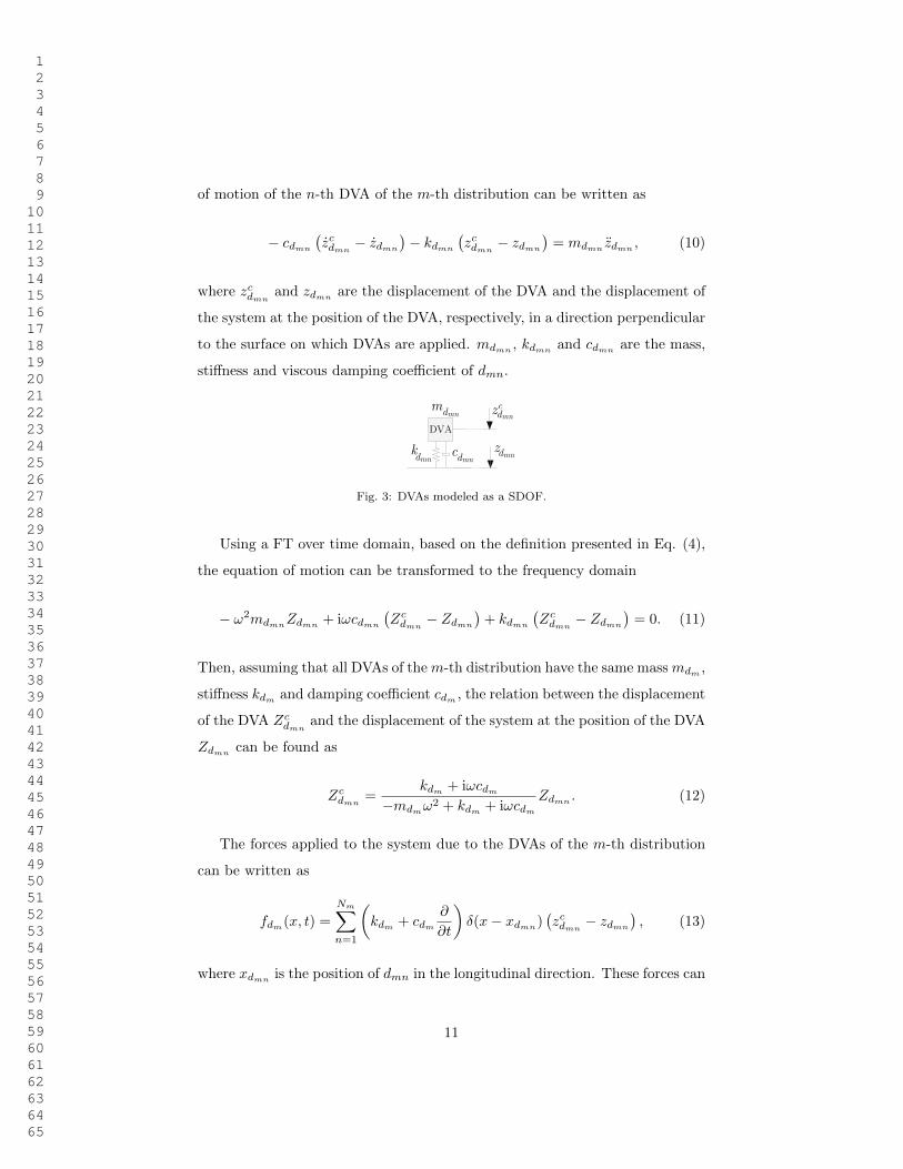
Considering each DVA as a SDOF system, as shown in Fig. 3, the equation
10
1 2 3 4 5 6 7 8 9 10 11 12 13 14 15 16 17 18 19 20 21 22 23 24 25 26 27 28 29 30 31 32 33 34 35 36 37 38 39 40 41 42 43 44 45 46 47 48 49 50 51 52 53 54 55 56 57 58 59 60 61 62 63 64 65
of motion of the n-th DVA of the m-th distribution can be written as
− cdmn
(zcdmn
− zdmn
)− kdmn
(zcdmn
− zdmn
)= mdmn
zdmn, (10)
where zcdmnand zdmn
are the displacement of the DVA and the displacement of
the system at the position of the DVA, respectively, in a direction perpendicular
to the surface on which DVAs are applied. mdmn , kdmn and cdmn are the mass,
stiffness and viscous damping coefficient of dmn.
dmn
c
dmn dmn
dmn
dmn
Fig. 3: DVAs modeled as a SDOF.
Using a FT over time domain, based on the definition presented in Eq. (4),
the equation of motion can be transformed to the frequency domain
− ω2mdmnZdmn
+ iωcdmn
(Zcdmn
− Zdmn
)+ kdmn
(Zcdmn
− Zdmn
)= 0. (11)
Then, assuming that all DVAs of the m-th distribution have the same mass mdm ,
stiffness kdm and damping coefficient cdm , the relation between the displacement
of the DVA Zcdmnand the displacement of the system at the position of the DVA
Zdmncan be found as
Zcdmn=
kdm + iωcdm−mdmω
2 + kdm + iωcdmZdmn . (12)
The forces applied to the system due to the DVAs of the m-th distribution
can be written as
fdm(x, t) =
Nm∑n=1
(kdm + cdm
∂
∂t
)δ(x− xdmn
)(zcdmn
− zdmn
), (13)
where xdmnis the position of dmn in the longitudinal direction. These forces can
11

1 2 3 4 5 6 7 8 9 10 11 12 13 14 15 16 17 18 19 20 21 22 23 24 25 26 27 28 29 30 31 32 33 34 35 36 37 38 39 40 41 42 43 44 45 46 47 48 49 50 51 52 53 54 55 56 57 58 59 60 61 62 63 64 65
be transformed to the wavenumber-frequency domain using Eq. (4), resulting
in
Fdm(kx, ω) =
Nm∑n=1
(kdm + iωcdm) eikxxdmn(Zcdmn
− Zdmn
). (14)
Finally, by introducing Eq. (12) into Eq. (14), the forces applied to the interior
floor by the DVAs can be rewritten as
Fdm(kx, ω) =
Nm∑n=1
k∗dmeikxxdmnZdmn, (15)
where
k∗dm =ω2mdm(kdm + iωcdm)
−ω2mdm + iωcdm + kdm. (16)
Therefore, the forces applied to the system by all M distributions of DVAs
can be written in matrix form as
Fd = ΓdK∗dZd, (17)
where
Fd =
Fd1
Fd2...
Fdm...
FdM
, Zd =
Zd1
Zd2...
Zdm...
ZdM
, (18)
where Zdm is a vector which contains the displacements of the system at the
positions of all the DVAs of the m-th distribution. The other matrices are
12

1 2 3 4 5 6 7 8 9 10 11 12 13 14 15 16 17 18 19 20 21 22 23 24 25 26 27 28 29 30 31 32 33 34 35 36 37 38 39 40 41 42 43 44 45 46 47 48 49 50 51 52 53 54 55 56 57 58 59 60 61 62 63 64 65
defined as
K∗d =
K∗d1
K∗d2. . .
K∗dm. . .
K∗dM
, (19)
where K∗dm is a Nm ×Nm matrix defined by k∗dmI; and
Γd =
Γd1
Γd2. . .
Γdm. . .
ΓdM
, (20)
where
Γdm ={
eikxxdm1 eikxxdm2 · · · eikxxdmNm
}. (21)
In the following, it is assumed that the force is applied only on one of the
rails. For the case of the two forces applied on the two rails, linear superposition
can be held. Moreover, the following derivation is based on the moving frame
of reference, as explained in Section 2. All the variables represented in the
frequency domain in this section are thus associated to the frequency ω. The
system’s response at the position of the DVAs can be obtained from
Zd = HdrFr + HddFd, (22)
where Hdr refers to the 2.5D Green’s function for the displacement of the system
at the DVAs positions due to a force on the rail seen in the moving frame of
reference in the absence of the DVAs; Fr is a force applied on the rails in the
13

1 2 3 4 5 6 7 8 9 10 11 12 13 14 15 16 17 18 19 20 21 22 23 24 25 26 27 28 29 30 31 32 33 34 35 36 37 38 39 40 41 42 43 44 45 46 47 48 49 50 51 52 53 54 55 56 57 58 59 60 61 62 63 64 65
moving frame of reference; and Hdd refers to the 2.5D Green’s function for
displacements of the system at the DVAs positions due to a force applied on the
DVAs positions. Replacing Fd with its equivalent from Eq. (17), Eq. (22) can
be rewritten in the form of 2.5D Green’s functions as
Hddr = Hdr + HddΓdK
∗dH
ddr, (23)
where Hddr is the 2.5D Green’s function that relates the displacement in the
DVAs positions with a force in the rails seen in the moving frame of reference in
the presence of the DVAs and Hddr is its inverse FT over the defined wavenumber
by using the same structure as Zd in Eq. (18). Transforming Eq. (23) to the
space-frequency domain by applying an inverse FT over the wavenumber and
evaluating the transformed equation at the positions of the DVAs one can obtain
the expression
Hddr = Hdr + HddK
∗dH
ddr, (24)
where
Hdr =
Hd1r
Hd2r
...
Hdmr
...
HdMr
, (25)
being Hdmr the receptances of the system at the DVAs positions of m-th dis-
tribution due to the force applied on one of the rails, defined as
Hdmr =1
vtHdmrΓ
Tdm , (26)
14

1 2 3 4 5 6 7 8 9 10 11 12 13 14 15 16 17 18 19 20 21 22 23 24 25 26 27 28 29 30 31 32 33 34 35 36 37 38 39 40 41 42 43 44 45 46 47 48 49 50 51 52 53 54 55 56 57 58 59 60 61 62 63 64 65
and where
Hdd =
Hd1d1 Hd1d2 · · · Hd1dp · · · Hd1dM
Hd2d1 Hd2d2 · · · Hd2dp · · · Hd2dM
......
. . ....
. . ....
Hdmd1 Hdmd2 · · · Hdmdp · · · HdmdM
......
. . ....
. . ....
HdMd1 HdMd2 · · · HdMdp · · · HdMdM
, (27)
being Hdmdp a Nm×Np matrix which contains receptance matrices of the system
at the DVAs positions of the m-th distribution due to the forces applied on the
system at the DVAs positions of the p-th distribution. Each element of these
matrices can be determined by
Hdmdp,jq =1
2π
∫ +∞
−∞Hdmdp,jqe
ikx(xjdm−xq
dp)dkx, (28)
j = 1, 2, . . . , Nm, q = 1, 2, . . . , Np, kxκx
where xjdm is the position of j-th DVA in the m-th distribution in the longitu-
dinal direction, and xqdp is the position of q-th DVA in the p-th distribution in
the longitudinal direction.
Finally, operating Eq. (24), the receptance of the system at the DVAs posi-
tions in the presence of the DVAs can be obtained as
Hddr = (I − HddKd)
−1Hdr. (29)
Having these receptances, one can obtain the 2.5D Green’s functions of the
system at any arbitrary position l due to the force applied at the rail in the
presence of the DVAs as
Hdlr = Hlr + HldΓdK
∗dH
ddr. (30)
where the Hlr refers to the 2.5D Green’s function of the system in the absence
15
1 2 3 4 5 6 7 8 9 10 11 12 13 14 15 16 17 18 19 20 21 22 23 24 25 26 27 28 29 30 31 32 33 34 35 36 37 38 39 40 41 42 43 44 45 46 47 48 49 50 51 52 53 54 55 56 57 58 59 60 61 62 63 64 65
of the DVAs. It is noteworthy that this methodology considers a strong coupling
approach, in which the DVAs affect the response of the rails.
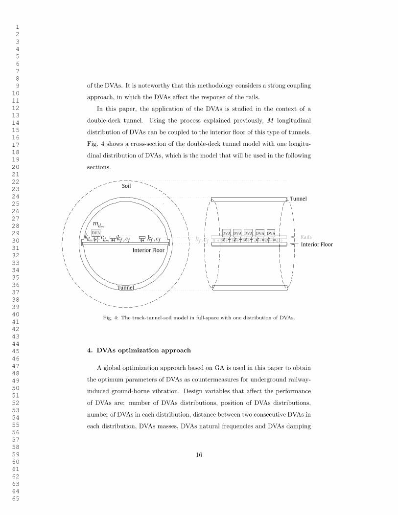
In this paper, the application of the DVAs is studied in the context of a
double-deck tunnel. Using the process explained previously, M longitudinal
distribution of DVAs can be coupled to the interior floor of this type of tunnels.
Fig. 4 shows a cross-section of the double-deck tunnel model with one longitu-
dinal distribution of DVAs, which is the model that will be used in the following
sections.
DVADVA
kf ,cf kf ,cf
m
k
dm
dm dmc kf ,cf
DVA DVA DVA DVA
Fig. 4: The track-tunnel-soil model in full-space with one distribution of DVAs.
4. DVAs optimization approach
A global optimization approach based on GA is used in this paper to obtain
the optimum parameters of DVAs as countermeasures for underground railway-
induced ground-borne vibration. Design variables that affect the performance
of DVAs are: number of DVAs distributions, position of DVAs distributions,
number of DVAs in each distribution, distance between two consecutive DVAs in
each distribution, DVAs masses, DVAs natural frequencies and DVAs damping
16
1 2 3 4 5 6 7 8 9 10 11 12 13 14 15 16 17 18 19 20 21 22 23 24 25 26 27 28 29 30 31 32 33 34 35 36 37 38 39 40 41 42 43 44 45 46 47 48 49 50 51 52 53 54 55 56 57 58 59 60 61 62 63 64 65
coefficients. In the optimization process, the effectiveness of DVAs is assessed
by their performance in minimizing energy flow radiated upwards.
The mean power flow radiated upwards from a tunnel towards nearby build-
ings was proposed by Hussein and Hunt [48] as a criterion to evaluate the per-
formance of vibration countermeasures. Studies of power flow and energy flow
that radiate upwards from a double-deck tunnel are presented by Clot et al. [49]
and [50], respectively. The radiated energy flow is the one used in this study
to assess the efficiency of DVAs and, in the following, it is explained how to
compute it.
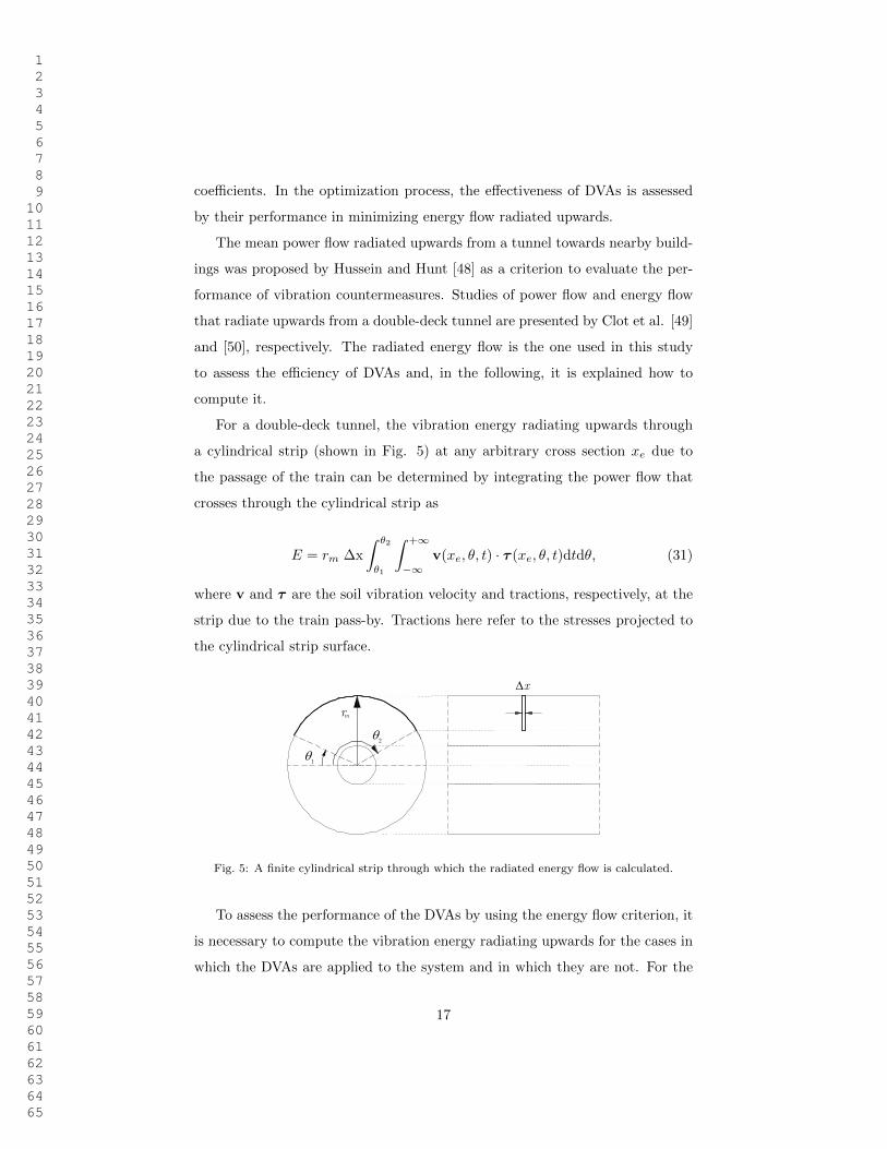
For a double-deck tunnel, the vibration energy radiating upwards through
a cylindrical strip (shown in Fig. 5) at any arbitrary cross section xe due to
the passage of the train can be determined by integrating the power flow that
crosses through the cylindrical strip as
E = rm ∆x
∫ θ2
θ1
∫ +∞
−∞v(xe, θ, t) · τ (xe, θ, t)dtdθ, (31)
where v and τ are the soil vibration velocity and tractions, respectively, at the
strip due to the train pass-by. Tractions here refer to the stresses projected to
the cylindrical strip surface.
xD
q1
q2
rm
Fig. 5: A finite cylindrical strip through which the radiated energy flow is calculated.
To assess the performance of the DVAs by using the energy flow criterion, it
is necessary to compute the vibration energy radiating upwards for the cases in
which the DVAs are applied to the system and in which they are not. For the
17

1 2 3 4 5 6 7 8 9 10 11 12 13 14 15 16 17 18 19 20 21 22 23 24 25 26 27 28 29 30 31 32 33 34 35 36 37 38 39 40 41 42 43 44 45 46 47 48 49 50 51 52 53 54 55 56 57 58 59 60 61 62 63 64 65
case without DVAs, the displacement and traction Green’s functions that relates
the response on the soil at the cylindrical strip due to a force applied on the i-th
rail can be obtained using the model explained in Subsection 2.1. These Green’s
functions can be used to obtain the response on the soil at the cylindrical strip
due a train pass-by by applying the formulation presented in Subsection 2.2
and, finally, to obtain the energy flow radiated upwards by the tunnel using Eq.
(31). For the case in which the DVAs are coupled to the tunnel’s interior floor,
the same procedure can be followed using the Green’s functions that accounts
for the DVAs application, which can be found by following Section 3.
5. Application and results
In this section, the efficiency of the application of the optimized DVAs on the
interior floor of the double-deck tunnel in minimizing the energy flow radiated
upwards by the tunnel is investigated. The considered mechanical properties
for the different subsystems are described first in Subsection 5.1. Then, in
Subsection 5.2, it is explained how the required Green’s function have been
computed, concerning the position of the receivers, possible position of DVAs
and the wavenumber-frequency sampling. The train pass-by response is com-
puted in Subsection 5.3. In Subsection 5.4, optimized parameters of DVAs to
minimize energy flow radiated upwards are computed by using the previously
explained optimization procedure, and the effects of the optimized DVAs are
discussed.
5.1. Parameters used to model subsystems
Two types of soil are considered, soft soil and hard soil. Their mechanical
parameters are summarized in Table 1. The purpose of using a low Youngs
modulus for the soft soil case is to assess the performance of the DVAs in an
extreme scenario. The mechanical and geometric parameters of the tunnel and
the interior floor can be found in Tables 2 and 3, respectively. Typical values of
reinforced concrete are used to model the tunnel and the interior floor.
18

1 2 3 4 5 6 7 8 9 10 11 12 13 14 15 16 17 18 19 20 21 22 23 24 25 26 27 28 29 30 31 32 33 34 35 36 37 38 39 40 41 42 43 44 45 46 47 48 49 50 51 52 53 54 55 56 57 58 59 60 61 62 63 64 65
Table 1: Mechanical parameters used to model the soil.
Soil parameters Values for soft soil Values for hard soil
Young modulus (MPa) 15 550
Density (kg m-3) 1600 2000
Poisson ratio (-) 0.49 0.3
P-wave damping ratio (-) 0.05 0.03
S-wave damping ratio (-) 0.05 0.03
Table 2: Mechanical parameters used to model the tunnel.
Tunnel parameters Values
Young modulus (GPa) 50
Density (kg m-3) 3000
Poisson ratio (-) 0.175
Thickness (m) 0.4
Interior radius (m) 5.65
Table 3: Mechanical parameters used to model the interior floor.
Interior floor parameters Values
Young modulus (GPa) 30
Density (kg m-3) 3000
Poisson ratio (-) 0.175
Thickness (m) 0.5
Width (m) 10.9
The track consists of two identical rails separated at a constant distance of
1.5 m and a continuous mass-less distribution of springs-dashpots as a model of
the fasteners. Their parameters are given in Tables 4 and 5.
19

1 2 3 4 5 6 7 8 9 10 11 12 13 14 15 16 17 18 19 20 21 22 23 24 25 26 27 28 29 30 31 32 33 34 35 36 37 38 39 40 41 42 43 44 45 46 47 48 49 50 51 52 53 54 55 56 57 58 59 60 61 62 63 64 65
Table 4: Mechanical parameters used to model the rail.
Rail parameters Values
Young modulus (GPa) 207
Density (kg m-3) 7850
Cross-section area (m2) 6.93·10-3
Second moment of area (m4) 23.5·10-6
Table 5: Mechanical parameters used to model the fastener.
Fasteners parameters Values
Uniformly distributed stiffness (N m-2) 20·106
Uniformly distributed viscous damping (N s m-2) 10·103
The considered train consists of two identical 3D models of the vehicle,
shown in Fig. 6. The distance between the wheels of a bogie, bogies of a same
car and bogies of two consecutive cars are 2.2 m, 15 m and 7 m, respectively.
The parameters of the 2D vehicle models referred to in Subsection 2.2 are: mw
represents the mass of the combined wheel and 1/2-axle system; mbog and Jbog
represent the mass and mass of inertia of a 1/2-bogie, respectively; kps and cps
represent the stiffness and viscous damping, respectively, of the primary vehicle
suspension system; mc and Jc represent the mass and mass of inertia of a 1/2-car
body; and kss and css represent the stiffness and viscous damping, respectively,
of the secondary vehicle suspension system. The values for these parameters
can be found in Table 6.
Fig. 6: Train configuration.
20

1 2 3 4 5 6 7 8 9 10 11 12 13 14 15 16 17 18 19 20 21 22 23 24 25 26 27 28 29 30 31 32 33 34 35 36 37 38 39 40 41 42 43 44 45 46 47 48 49 50 51 52 53 54 55 56 57 58 59 60 61 62 63 64 65
Table 6: Mechanical parameters used to model the train.
Vehicle parameters Values Vehicle parameters Values
mw (kg) 950 kH (N m-1) 109
mbog (kg) 4700 kps (N m-1) 14·105
Jbog (kg m2) 1300 cps (N s m-1) 9·103
mc (kg) 22500 kss (N m-1) 6·105
Jc (kg m2) 55·104 css (N s m-1) 21·103
5.2. Computation of the Green’s functions
The track-tunnel-soil model presented in Subsection 2.1, along with the pa-
rameters of the subsystems given in the previous section, is used to compute
the Green’s functions required for coupling the vehicle and DVAs to the track
and the interior floor, respectively, and for computing the energy flow radiated
upwards due to the passage of the train. The computation of the energy flow
radiated upwards takes into account a set of receivers on the soil at a semicircle
concentric with the tunnel and with the radius rs = 12 m. A total amount
of 21 receivers with an angular resolution of 9π/20 rad are spread out across
the semicircle. For the coupling between the DVAs and the interior floor, 20
receivers along the y coordinate over the interior floor are considered. They are
the possible DVAs positions that are considered in the optimization process.
These receivers are equidistantly spread out across the interior floor considering
a space resolution of 0.5 m, and a distance of 0.5 m from each edge of the in-
terior floor. The receivers in the soil and the interior floor, denoted by dm and
sl, respectively, are shown in Fig. 7.
21

1 2 3 4 5 6 7 8 9 10 11 12 13 14 15 16 17 18 19 20 21 22 23 24 25 26 27 28 29 30 31 32 33 34 35 36 37 38 39 40 41 42 43 44 45 46 47 48 49 50 51 52 53 54 55 56 57 58 59 60 61 62 63 64 65
d1 d2 d20s
21
sl
s20
s1
s2
r2r1
dmy
z
x
rs
Fig. 7: Geometrical scheme of the receivers located at the soil and at the interior floor.
The Green’s functions have been computed for the moving loads with the
speeds of vt = 20 and 25 m s−1, which represent typical and maximum train
speeds for underground urban railways, respectively. The wavenumber-frequency
sampling is developed assuming a maximum frequency of interest, seen from a
fixed frame of reference, of ωmax = 2π80 rad/s. To compute the corresponding
maximum frequency of interest seen from the perspective of the moving frame
of reference ωmax, the expression
ωmax = ωmax
(1 +
vtβ
), (32)
from [44] is used here, where β is the speed of S-waves in the soil.
It is proposed to computationally solve Eqs. (8) or (9) by using an inverse
fast Fourier Transform (ifft) routine. Consider that the train response is
computed at x = 0. Taking into account that the moving frame of reference is
defined as x = x − vtt, one can define the sampling vectors for x and t in the
basis of the fft as
xn = −∆x[−N/2 . . . n− 1 −N/2 . . . N/2 − 1
](33)
22

1 2 3 4 5 6 7 8 9 10 11 12 13 14 15 16 17 18 19 20 21 22 23 24 25 26 27 28 29 30 31 32 33 34 35 36 37 38 39 40 41 42 43 44 45 46 47 48 49 50 51 52 53 54 55 56 57 58 59 60 61 62 63 64 65
and
tn = ∆t[−N/2 . . . n− 1 −N/2 . . . N/2 − 1
], (34)
respectively, where ∆x = vt∆t. Thus, the corresponding sampling for kx
and ω should be
kxn = −∆kx
[−N/2 . . . n− 1 −N/2 . . . N/2 − 1
], (35)
and
ωn = ∆ω[−N/2 . . . n− 1 −N/2 . . . N/2 − 1
], (36)
respectively, where ∆ω = vt∆kx. Applying a 2D ifft over this sampling strat-
egy, the diagonal of the resulting 2D matrix for the specific receiver contains
the time response at x = 0.
The assumption for which the train response is computed at x = 0 comes
from the fact that, in pure 2.5D models, the time response at any arbitrary x is
always the same as the one computed at x = 0 but delayed in time. However,
when the DVAs are coupled to the system, the resulting model is no longer
longitudinally invariant since it includes a periodical system, which induces a
periodical behavior on the time response. Therefore, x = 0 represents only
one of the possible time responses existing within a periodicity. However, the
soil response is not significantly affected by this periodical behaviour due to the
distance between the track and the receivers in comparison with the longitudinal
distance between DVAs. Thus, x = 0 is taken as the representative time signal
for the train response.
5.3. Train pass-by response
In this study, the unevenness profiles of the two rails are held to be uncor-
related. As shown by Ntotsios et al. [46], unevenness spectral content of wave-
lengths shorter than 3 m should be considered uncorrelated. The train speeds
studied in this paper imply that for frequencies larger than ≈ 8 Hz (most of
the frequency range of interest for railway-induced vibrations), the unevenness
23

1 2 3 4 5 6 7 8 9 10 11 12 13 14 15 16 17 18 19 20 21 22 23 24 25 26 27 28 29 30 31 32 33 34 35 36 37 38 39 40 41 42 43 44 45 46 47 48 49 50 51 52 53 54 55 56 57 58 59 60 61 62 63 64 65
profiles of the two rails are deemed to be uncorrelated. They are modeled using
a stochastic random process that is characterized by its power spectral density
(PSD) [51] which depends on the rail quality. According to the Federal Rail-
road Administration (FRA), the unevenness of the rails can be grouped into six
classes depending on the rail quality. Class 3 track is used in here.
Fig. 8 shows the time histories of the vertical rail velocity at x = 0 of the
left rail, in the absence of DVAs, due to the train passage at speeds of 20 and
25 m s−1. The passage of the train, which has a total of eight axles, can be
seen through the eight peaks appearing in the figure. It is apparent that the
vertical rail velocity of the rail grows by increasing the train speed. Furthermore,
considering the velocity and the length of the train, the time it takes for the
train to pass corresponds to the distance between the peaks in time.
-4 -2 0 2 4
Time [s]
-0.15
-0.1
-0.05
0
0.05
0.1
0.15
Ve
locity [
m/s
]
(a)
-4 -2 0 2 4
Time [s]
-0.15
-0.1
-0.05
0
0.05
0.1
0.15
Ve
locity [
m/s
]
(b)
Fig. 8: Time history of the vertical velocity of the left rail due to the train passing at speedsof (a) vt = 20 m s−1 and (b) vt = 25 m s−1.
Fig. 9 shows the time history of the radial velocity of the hard soil at the
receiver s10, i.e. located at θ = π/2 and rs = 12 m, due to train passing
at speeds of 20 and 25 m s−1. In this case, due to the distance between the
receiver and the track, the passage of the train axles cannot be clearly identified
as compared with the rail response.
24

1 2 3 4 5 6 7 8 9 10 11 12 13 14 15 16 17 18 19 20 21 22 23 24 25 26 27 28 29 30 31 32 33 34 35 36 37 38 39 40 41 42 43 44 45 46 47 48 49 50 51 52 53 54 55 56 57 58 59 60 61 62 63 64 65
-4 -2 0 2 4
Time [s]
-3
-2
-1
0
1
2
3
Ve
locity [
m/s
]
×10-4 (a)
-4 -2 0 2 4
Time [s]
-3
-2
-1
0
1
2
3
Ve
locity [
m/s
]
×10-4 (b)
Fig. 9: Time history of the radial velocity of the soil at θ = π/2 and rs = 12 m due to thetrain passing at speeds of (a) vt = 20 m s−1 and (b) vt = 25 m s−1.
Fig. 10 shows the frequency spectrum of the radial velocity for the hard and
soft soil at the receiver s10, located at θ = π/2 rad and rs = 12 m, due to the
passage of the train at the speeds of 20 and 25 m s−1. It can be observed that
the dominant spectral content is in a narrow frequency band for the four cases.
Observing the same behavior at the other receivers implies that DVAs would be
suitable vibration isolation measures. However, they would be less efficient for
the soft soil cases as the dominant frequency band is wider.
5.4. Optimum parameters of DVAs
Only one distribution of DVAs is considered in this study. Moreover, the
distance between any two consecutive DVAs in a distribution is assumed to be
the same. The DVAs in a distribution are considered to have the same mass. Its
value, together with the minimum distance between the DVAs and the number
of them, are defined in the pre-design stage (common practice in designing DVAs
[52]) by ensuring that the static tensions to which the interior floor is subjected
would stay approximately unchanged after adding DVAs. This bound is applied
in order to avoid structural integrity problems. Thus, the transverse position
of DVAs distribution at the interior floor, the distance between two consecutive
25

1 2 3 4 5 6 7 8 9 10 11 12 13 14 15 16 17 18 19 20 21 22 23 24 25 26 27 28 29 30 31 32 33 34 35 36 37 38 39 40 41 42 43 44 45 46 47 48 49 50 51 52 53 54 55 56 57 58 59 60 61 62 63 64 65
20 40 60 80 100
Frequency [Hz]
0
0.5
1
1.5V
elo
city [m
/s/H
z]
×10-4 (a)
20 40 60 80 100
Frequency [Hz]
0
0.5
1
1.5
Velo
city [m
/s/H
z]
×10-4 (b)
20 40 60 80 100
Frequency [Hz]
0
0.5
1
1.5
Velo
city [m
/s/H
z]
×10-4 (c)
20 40 60 80 100
Frequency [Hz]
0
0.5
1
1.5
Velo
city [m
/s/H
z]
×10-4 (d)
Fig. 10: Frequency spectrum of the radial velocity for the hard soil (top) and soft soil (bottom)at θ = π/2 rad and rs = 12 m due to the train passing at speeds of (a,c) vt = 20 m s−1 and(b,d) vt = 25 m s−1.
DVAs, the natural frequency of the DVAs and viscous damping of the DVAs are
defined as design variables in the optimization process.
In this study, the Matlab Global Optimization Toolbox [53] is employed.
This toolbox provides functions for finding parameters which minimize an ob-
jective while satisfying a set of constraints. The optimization problem set up in-
cludes choosing a solver, defining the objective functions and constraints, defin-
26

1 2 3 4 5 6 7 8 9 10 11 12 13 14 15 16 17 18 19 20 21 22 23 24 25 26 27 28 29 30 31 32 33 34 35 36 37 38 39 40 41 42 43 44 45 46 47 48 49 50 51 52 53 54 55 56 57 58 59 60 61 62 63 64 65
ing optimization options and including parallel processing. In this study, ga
(genetic algorithm of MATLAB) has been used as the solver, and the energy
flow radiated upwards in the presence of the DVAs has been defined as the ob-
jective function. Among bound constraints and linear/non-linear constraints,
only the former has been considered. These constraints limit the range from
which the design variables can be chosen in the optimization problem. In the
ga solver, a set of options can be specified to obtain data from the algorithm
while it is running, to drive a random selection of the possible candidates for
the solution and to define conditions to terminate the optimization process. In
this study, the approach which makes the selection of the candidates being more
random than driven has been employed. The maximum number of iterations for
the algorithm to perform is used as a condition to terminate the optimization
process and it has been defined as triple that of the default value proposed by
the algorithm, which is 50. In short, as a general work flow of this algorithm,
ga searches for the optimal values of DVAs parameters that can minimize the
energy flow radiated upwards from the cylindrical strip due to the passage of
the train by considering the bounds constraints. The upper and lower bounds
of the design variables and the value of the parameters defined in the pre-design
stage are given in the following:
1. Number of DVAs distributions M : Only one longitudinal distribution of
DVAs is considered.
2. Transverse position of DVAs distribution yd. It can be chosen from 20
possible positions defined previously in Subsection 5.2.
3. Distance between two consecutive DVAs ld: It is defined as a discrete
variable, which can be chosen from 1 m to 8 m as the lower and upper
bounds of this design variable, respectively, with a space step of 0.5 m.
The space step has been restricted to 0.5 m because of the size of the
DVAs to be used.
4. The mass of the DVAs md: It is defined in the pre-design stage. All DVAs
27
1 2 3 4 5 6 7 8 9 10 11 12 13 14 15 16 17 18 19 20 21 22 23 24 25 26 27 28 29 30 31 32 33 34 35 36 37 38 39 40 41 42 43 44 45 46 47 48 49 50 51 52 53 54 55 56 57 58 59 60 61 62 63 64 65
in a distribution are assumed to have the same mass of 800 kg.
5. Number of DVAs in a distribution N : It is also defined in the pre-design
stage, taking a value of 15 DVAs.
6. The natural frequency of the DVAs fd: It is defined as a discrete variable
that can be chosen from the values of the fixed frame frequency (i.e. seen
from the fixed frame of reference) given by the wavenumber-frequency
sampling defined in Subsection 5.2.
7. The viscous damping of the DVAs cd: It is defined as a discrete variable
with lower and upper bounds of 5 kN s m−1 and 500 kN s m−1, respec-
tively. It is considered to be a total amount of 316 possible values linearly
distributed between the defined bounds.
An optimization process based on GA has been carried out to minimize the
energy flow radiated upwards due to the application of a distribution of DVAs.
The following four cases have been studied: Case H25: hard soil and train speed
of vt = 25 m s−1; Case H20: hard soil and train speed of vt = 20 m s−1; Case
S20: soft soil and train speed of vt = 20 m s−1 and Case S25: soft soil and train
speed of vt = 25 m s−1. The resulting optimum values of the DVAs parameters
and the associated insertion loss (IL) on the radiated energy flow are presented
in Table 7. The IL was computed as
IL = 10 log10
(E
E′
), (37)
where E and E′ represent the radiated energy without and with the application
of the DVAs.
28

1 2 3 4 5 6 7 8 9 10 11 12 13 14 15 16 17 18 19 20 21 22 23 24 25 26 27 28 29 30 31 32 33 34 35 36 37 38 39 40 41 42 43 44 45 46 47 48 49 50 51 52 53 54 55 56 57 58 59 60 61 62 63 64 65
Table 7: The optimum values of DVAs parameters and resulting IL.
Case yd (m) ld (m) fd (Hz) cd (kN s m−1) IL (dB)
H20 3.55 7.5 31.52 14.09 6.2
H25 -2.45 4.5 28.83 27.07 6.6
S20 1.05 7 31.17 20.65 5.3
S25 -3.45 6 31.6 27.76 5.8
Fig. 11 shows the mean power flow radiated upwards from the cylindrical
strip with and without DVAs in the time domain for the four studied cases. The
total radiated energy with and without DVAs is also given for each case. This
mean power flow has been computed using the velocities and tractions over the
cylindrical strip at xe = 0, which is defined in accordance with the space-time
sampling previously defined in Subsection 5.2. The expression to compute the
mean power flow can be derived from Eq. (31) and it is
P (t) = rm ∆x
∫ θ2
θ1
v(xe, θ, t) · τ (xe, θ, t)dθ. (38)
As generally expected, the radiated energy increases for both soft and hard
soil when the speed of the train increases. The comparison of the radiated
power flow or the total radiated energy with and without the application of
DVAs indicates that using DVAs results in a notable decrease in radiated power
flow or total radiated energy for all studied cases. For all the studied cases,
Fig. 11 shows that the mean power flow becomes negative-valued at specific
instants of time. This behavior of the mean power flow radiated upwards by
a double-deck tunnel was previously observed by Clot [54] for the case of a
quasi-static point load. A meaningful explanation of this phenomenon is that
the elastic surface waves that travel along the tunnel cavity exhibit a particle
motion very similar to the one presented by Rayleigh surface waves [55]. This
close resemblance indicates the existence of elliptical particle motion of the soil
close to the tunnel structure. This means that at some time intervals there are
particle motions of the soil toward the tunnel rather than away from it. This
29

1 2 3 4 5 6 7 8 9 10 11 12 13 14 15 16 17 18 19 20 21 22 23 24 25 26 27 28 29 30 31 32 33 34 35 36 37 38 39 40 41 42 43 44 45 46 47 48 49 50 51 52 53 54 55 56 57 58 59 60 61 62 63 64 65
-4 -2 0 2 4
Time [s]
-3
-2
-1
0
1
2
3
4
5
6P
ow
er
[W]
×10-2 (a)
E = 0.0209 J
E′= 0.0050 J
-4 -2 0 2 4
Time [s]
-3
-2
-1
0
1
2
3
4
5
6
Pow
er
[W]
×10-2 (b)
E = 0.0344 J
E′= 0.0075 J
-4 -2 0 2 4
Time [s]
-3
-2
-1
0
1
2
3
4
5
6
Pow
er
[W]
×10-2 (c)
E = 0.0196 J
E′= 0.0058 J
-4 -2 0 2 4
Time [s]
-3
-2
-1
0
1
2
3
4
5
6
Pow
er
[W]
×10-2 (d)
E = 0.0368 J
E′= 0.0097 J
Fig. 11: Mean power flow radiated upwards over the cylindrical strip in the time domain forthe cases (a) H20, (b) H25, (c) S20 and (d) S25. The grey and black lines represent the resultswith and without DVAs, respectively. The total radiated energy is presented for each case.
results in negative radiated vibration power flow if the positive power flow is
defined as the power radiated away from the tunnel.
Fig. 12 shows the energy spectral density (ESD) of the previously computed
mean power flow, with and without DVAs, for the four studied cases. As ex-
pected, the results of computing the total radiated energy using ESD is the
same value previously achieved from the mean power flow in the time domain.
30

1 2 3 4 5 6 7 8 9 10 11 12 13 14 15 16 17 18 19 20 21 22 23 24 25 26 27 28 29 30 31 32 33 34 35 36 37 38 39 40 41 42 43 44 45 46 47 48 49 50 51 52 53 54 55 56 57 58 59 60 61 62 63 64 65
10 20 30 40 50 60 70 80
Frequency [Hz]
0
0.5
1
1.5
2
2.5
3
3.5E
SD
[J/H
z]
×10-2 (a)
E = 0.0209 J
E′= 0.0050 J
10 20 30 40 50 60 70 80
Frequency [Hz]
0
0.5
1
1.5
2
2.5
3
3.5
ES
D [J/H
z]
×10-2 (b)
E = 0.0344 J
E′= 0.0075 J
10 20 30 40 50 60 70 80
Frequency [Hz]
0
0.5
1
1.5
2
2.5
3
3.5
ES
D [J/H
z]
×10-2 (c)
E = 0.0196 J
E′= 0.0058 J
10 20 30 40 50 60 70 80
Frequency [Hz]
0
0.5
1
1.5
2
2.5
3
3.5
ES
D [J/H
z]
×10-2 (d)
E = 0.0368 J
E′= 0.0097 J
Fig. 12: ESD for cases (a) H20, (b) H25, (c) S20 and (d) S25. The grey and black linesrepresent the results with and without DVAs, respectively. The total radiated energy is alsopresented for each case.
It can be observed in Fig. 12 that the most significant energy content is
concentrated in a frequency range between 25 to 35 Hz. It is noteworthy that
the optimized natural frequencies of DVAs have been obtained in this range of
frequency, which makes them effective in minimizing the radiated energy. The
range of frequency in which most of the energy content is found and at which
the DVAs are effective can be seen more clearly in Fig. 13, which represents
31
1 2 3 4 5 6 7 8 9 10 11 12 13 14 15 16 17 18 19 20 21 22 23 24 25 26 27 28 29 30 31 32 33 34 35 36 37 38 39 40 41 42 43 44 45 46 47 48 49 50 51 52 53 54 55 56 57 58 59 60 61 62 63 64 65
energy spectrum in one-third octave band for the considered cases with and
without application of DVAs. The presented octave bands are normalized with
the length of the time signal, which is 8.54 seconds.
1 2 4 8 16 31.5 63
Frequency [Hz]
-35
-30
-25
-20
-15
-10
-5
Energ
y s
pectr
um
[dB
]
(a)
1 2 4 8 16 31.5 63
Frequency [Hz]
-35
-30
-25
-20
-15
-10
-5
Energ
y s
pectr
um
[dB
]
(b)
1 2 4 8 16 31.5 63
Frequency [Hz]
-35
-30
-25
-20
-15
-10
-5
Energ
y s
pectr
um
[d
B]
(c)
1 2 4 8 16 31.5 63
Frequency [Hz]
-35
-30
-25
-20
-15
-10
-5
Energ
y s
pectr
um
[d
B]
(d)
Fig. 13: One-third octave bands spectrum of energy in dB (dB reference 1 J) for cases (a)H20, (b) H25, (c) S20 and (d) S25. The grey and black lines represent the results with andwithout DVAs, respectively.
In order to study the radiation pattern of the energy flow, the energy radiated
through the cylindrical strip has been computed as a function of θ, for all studied
32

1 2 3 4 5 6 7 8 9 10 11 12 13 14 15 16 17 18 19 20 21 22 23 24 25 26 27 28 29 30 31 32 33 34 35 36 37 38 39 40 41 42 43 44 45 46 47 48 49 50 51 52 53 54 55 56 57 58 59 60 61 62 63 64 65
cases and with and without the application of DVAs, using
E(θ) = rm ∆x
∫ +∞
−∞v(0, θ, t) · τ (0, θ, t)dt. (39)
The results are shown in Fig. 14. One thing to note is that depending on
the type of the soil, the energy flow radiation pattern would differ. For hard
soil cases, the energy mostly radiates over the center of the strip, however,
for the soft soil cases, it radiates mostly over the sides of the strip. For both
cases, DVAs are significantly affecting the θ distribution of the radiation pattern.
This is because the mode shapes of the interior floor, which are modified by
the application of the DVAs, are strongly related with the radiation pattern
distribution, as discussed previously by Clot et al. [49] in a 2D power flow
analysis of the double-deck tunnel subjected to a harmonic line load.
0
/6
/3
/2
2 /3
5 /6
0
0.005
0.009
0.013
(a)
0
/6
/3
/2
2 /3
5 /6
0
0.005
0.009
0.013
(b)
0
/6
/3
/2
2 /3
5 /6
0
0.005
0.009
0.013
(c)
0
/6
/3
/2
2 /3
5 /6
0
0.005
0.009
0.013
(d)
Fig. 14: Energy radiated over cylindrical strip in J as a function of θ for cases (a) H20, (b)H25, (c) S20 and (d) S25. The grey and black lines represent the results with and withoutDVAs, respectively.
In order to investigate the relation between the natural frequency of the
optimal DVAs and the dynamical behavior of the original system, two figures
33

1 2 3 4 5 6 7 8 9 10 11 12 13 14 15 16 17 18 19 20 21 22 23 24 25 26 27 28 29 30 31 32 33 34 35 36 37 38 39 40 41 42 43 44 45 46 47 48 49 50 51 52 53 54 55 56 57 58 59 60 61 62 63 64 65
are presented. On the one hand, Fig. 15 shows the radial velocity Green’s
functions of the hard soil case at three receivers located at θ = 0, θ = π/2
and θ = π rad, and at a radius of 12 m due to the force applied on the right
rail. The red areas show local maximums of the velocity Green’s functions
and they represent an approximation to the dispersion curves of the system.
From this approximation, three propagation modes of the interior floor coupled
to the tunnel-soil system can be observed: the first and the third are anti-
symmetric (not observed at θ = π/2) and the second is symmetric (the only
one appearing at θ = π/2). The inclined dashed black lines plotted in Fig.
15 represent combinations of kx and ω of constant ω for the specific speed of
25 m s−1. On the other hand, Fig. 16 shows dynamic wheel-rail interaction
forces for the same case study but considering 20 m s−1 and 25 m s−1. For
both figures, the computations have been done without considering coupled
DVAs. Comparing these two figures with the results shown in Table 7, where
the natural frequency of the optimal DVAs for the hard soil case is 31.52 Hz for
vt = 20 m s−1 and 28.83 Hz for vt = 25 m s−1, one can observe that the DVAs
are targeting the second propagation mode of the track-interior floor-tunnel-soil
system. This can be deduced because of two reasons: firstly, the inclined black
lines of constant ω have a slope far from the tangents to the dispersion curves
except for wavenumbers close to zero, resulting in that the frequency associated
to these propagation modes is mostly the one of the 2D problem; secondly, the
contact forces have a significant amount of spectral energy close to the resonance
frequency associated to the second propagation mode for the 2D case.
34

1 2 3 4 5 6 7 8 9 10 11 12 13 14 15 16 17 18 19 20 21 22 23 24 25 26 27 28 29 30 31 32 33 34 35 36 37 38 39 40 41 42 43 44 45 46 47 48 49 50 51 52 53 54 55 56 57 58 59 60 61 62 63 64 65
(a)
-1 0 1
Wavenumber [rad/m]
10
20
30
40
50
60
70
80
90F
req
ue
ncy [
Hz]
-400
-325
-250
-175
-100(b)
-1 0 1
Wavenumber [rad/m]
10
20
30
40
50
60
70
80
90
Fre
qu
en
cy [
Hz]
(c)
-1 0 1
Wavenumber [rad/m]
10
20
30
40
50
60
70
80
90
Fre
qu
en
cy [
Hz]
Fig. 15: The radial velocity Green’s functions of the hard soil in dB (dB reference 1 m N−1s−1)at the receivers located at rs = 12 m and (a) θ = 0, (b) θ = π/2 rad and (c) θ = π rad forvt = 25 m s−1. Inclined dashed black lines denote points of constant ω for the specific speedof 25 m s−1.
0 10 20 30 40 50 60 70 80 90
Frequency [Hz]
0
0.5
1
1.5
2
Co
nta
ct
forc
e [
N/H
z]
×104
Fig. 16: Contact forces caused by wheel-rail interaction associated to vt = 20 m s−1 (grey)and vt = 25 m s−1 (black).
The effect of the DVAs on the dynamic response of the rails is also studied.
Fig. 17 shows the one-third octave band spectrum of the vertical velocity of
35

1 2 3 4 5 6 7 8 9 10 11 12 13 14 15 16 17 18 19 20 21 22 23 24 25 26 27 28 29 30 31 32 33 34 35 36 37 38 39 40 41 42 43 44 45 46 47 48 49 50 51 52 53 54 55 56 57 58 59 60 61 62 63 64 65
the left rail with and without DVAs, for two different train speeds. It can
be seen from the figures that the application of DVAs on the interior floor of
the tunnel has little effect on the dynamic response of the track. Because of
that, the train-track dynamic forces can be computed before the optimization
process, only once. If the track is already constructed, these forces can be
obtained using a hybrid approach [12] that enhance the accuracy of the DVAs
efficiency prediction. However, it is important to highlight that this result is only
associated to the present problem parameters. In cases where the DVAs natural
frequency is similar to the rail/fasteners natural frequency, this conclusion is no
longer valid.
1 2 4 8 16 31.5 63 125
Frequency [Hz]
50
60
70
80
90
100
110
Ve
locity [
dB
]
(a)
1 2 4 8 16 31.5 63 125
Frequency [Hz]
50
60
70
80
90
100
110V
elo
city [
dB
](b)
Fig. 17: One-third octave band spectrum of the vertical velocity of the left rail in dB (dBreference 10−8 m s−1) for the train speeds of (a) vt = 20 m s−1 and (b) vt = 25 m s−1. Thegrey and black lines represent the results with and without DVAs, respectively.
6. Conclusions
The main objective of this paper is to evaluate the efficiency of the appli-
cation of DVAs in a double-deck tunnel to mitigate the underground railway-
induced ground-borne vibration. The total energy flow radiated upwards by a
double-deck tunnel due to train pass-by has been considered to be the criterion
36

1 2 3 4 5 6 7 8 9 10 11 12 13 14 15 16 17 18 19 20 21 22 23 24 25 26 27 28 29 30 31 32 33 34 35 36 37 38 39 40 41 42 43 44 45 46 47 48 49 50 51 52 53 54 55 56 57 58 59 60 61 62 63 64 65
to assess the performance of DVAs. A semi-analytical model of a double-deck
tunnel embedded in a full-space has been used to compute the energy flow ra-
diated upwards by the double-deck tunnel due to the train pass-by over a track
system located at its interior floor. A methodology to couple DVAs to any sub-
system of a railway infrastructure has been explained and was then employed to
couple DVAs to the interior floor of a double-deck tunnel. Taking into account
the crucial role of the DVAs parameter in their performance, a global optimiza-
tion approach based on GA has been used to obtain the optimal parameters of
DVAs to minimize the total radiated energy.
The performance of one longitudinal distribution of DVAs has been evalu-
ated for two different types of soil and two different train speeds. In all of the
four cases, they have been found to be efficient in reducing the total radiated
energy flow by the tunnel. The obtained insertion loss of the total radiated
energy flow due to the application of DVAs for the four cases shows that the
harder the soil is and the faster the train, the more effective are the optimized
DVAs. In the case of the hard soil and the train speed of 25 m/s, a reduction
of 6.6 dB in the total radiated energy flow has been achieved. The results show
that DVAs provide significant vibration attenuation benefits by tuning their
optimum natural frequencies to be set down in the range of frequency where
most of the energy spectral content is concentrated. Another finding is that
the energy flow radiation pattern from the tunnel is strongly modified after
the application of the DVAs, as they modify the mode shapes of the interior
floor. However, the application of DVAs does not considerably affect the dy-
namic response of the rails. It is expected that using more than one longitudinal
distribution of DVAs would result in a greater reduction in the total radiated
energy flow. It can be noted that DVAs would be a more cost-effective solution
for existing underground railway networks than, for example, vibration isola-
tion screens or building base isolation, as their implementation would be cheaper
than other vibration countermeasures. Noteworthy, it is expected that DVAs
as countermeasures for railway-induced ground-borne vibrations would be gen-
erally more effective for the cases with a sharper vibration frequency spectra of
37
1 2 3 4 5 6 7 8 9 10 11 12 13 14 15 16 17 18 19 20 21 22 23 24 25 26 27 28 29 30 31 32 33 34 35 36 37 38 39 40 41 42 43 44 45 46 47 48 49 50 51 52 53 54 55 56 57 58 59 60 61 62 63 64 65
the tunnel response (like the ones in double-deck tunnels) rather than the ones
with smooth vibration frequency spectra (like the ones in conventional tunnels).
Nevertheless, their effectiveness for conventional tunnels and at-grade railway
infrastructures is not studied in detail yet.
Acknowledgments
This work has been carried out in the context of the Industrial Doctorates
Plan, with the financial support of Agencia de Gestio d’Ajuts Universitaris i
de Recerca (AGAUR) from Generalitat de Catalunya and the company AV In-
genieros. It was developed in a partnership with Universitat Politecnica de
Catalunya (UPC). The authors would like to extend their gratitude to the ISI-
BUR project, Innovative Solutions for the Isolation of Buildings from Under-
ground Railway-induced Vibrations, funded by Ministerio de Economıa y Com-
petitivad de Espana (TRA2014 52718-R). The second author also wants to ac-
knowledge the funds provided by the NVTRail project, Noise and Vibrations in-
duced by railway traffic in tunnels: an integrated approach, with grant reference
POCI-01-0145-FEDER-029577, funded by FEDER through COMPETE2020
(Programa Operacional Competitividade e Internacionalizacao (POCI)) and by
national funds (PIDDAC) through FCT/MCTES.
References
[1] G. Lombaert, G. Degrande, B. Vanhauwere, B. Vandeborght, S. Francois,
The control of ground-borne vibrations from railway traffic by means of
continuous floating slabs, Journal of Sound and Vibration 297 (2006) 946–
961.
[2] P. Alves Costa, R. Calcada, A. Silva Cardoso, Ballast mats for the re-
duction of railway traffic vibrations. Numerical study, Soil Dynamics and
Earthquake Engineering 42 (2012) 137–150.
38

1 2 3 4 5 6 7 8 9 10 11 12 13 14 15 16 17 18 19 20 21 22 23 24 25 26 27 28 29 30 31 32 33 34 35 36 37 38 39 40 41 42 43 44 45 46 47 48 49 50 51 52 53 54 55 56 57 58 59 60 61 62 63 64 65
[3] J. Talbot, W. Hamad, H. Hunt, Base-isolated buildings and the added-
mass effect, in: Proceedings of ISMA 2014-International Conference on
Noise and Vibration Engineering and USD 2014-International Conference
on Uncertainty in Structural Dynamics, 2014, pp. 943–954.
[4] J. Talbot, H. Hunt, On the performance of base-isolated buildings, Building
Acoustics 7 (2000) 163–178.
[5] L. Andersen, S. R. Nielsen, Reduction of ground vibration by means of
barriers or soil improvement along a railway track, Soil Dynamics and
Earthquake Engineering 25 (2005) 701–716.
[6] P. Coulier, S. Francois, G. Degrande, G. Lombaert, Subgrade stiffening next
to the track as a wave impeding barrier for railway induced vibrations, Soil
Dynamics and Earthquake Engineering 48 (2013) 119–131.
[7] X. Sheng, C. J. C. Jones, D. J. Thompson, Prediction of ground vibration
from trains using the wavenumber finite and boundary element methods,
Journal of Sound and Vibration 293 (2006) 575–586.
[8] S. Francois, M. Schevenels, P. Galvın, G. Lombaert, G. Degrande, A 2.5D
coupled FE-BE methodology for the dynamic interaction between longitu-
dinally invariant structures and a layered halfspace, Computer Methods in
Applied Mechanics and Engineering 199 (2010) 1536–1548.
[9] P. Alves Costa, R. Calcada, A. Silva Cardoso, Track-ground vibrations
induced by railway traffic: In-situ measurements and validation of a 2.5D
FEM-BEM model, Soil Dynamics and Earthquake Engineering 32 (2012)
111–128.
[10] P. Amado-Mendes, P. Alves Costa, L. M. C. Godinho, P. Lopes, 2.5D MFS-
FEM model for the prediction of vibrations due to underground railway
traffic, Engineering Structures 104 (2015) 141–154.
39

1 2 3 4 5 6 7 8 9 10 11 12 13 14 15 16 17 18 19 20 21 22 23 24 25 26 27 28 29 30 31 32 33 34 35 36 37 38 39 40 41 42 43 44 45 46 47 48 49 50 51 52 53 54 55 56 57 58 59 60 61 62 63 64 65
[11] J. C. O. Nielsen, G. Lombaert, S. Francois, A hybrid model for prediction
of ground-borne vibration due to discrete wheel/rail irregularities, Journal
of Sound and Vibration 345 (2015) 103–120.
[12] K. A. Kuo, H. Verbraken, G. Degrande, G. Lombaert, Hybrid predictions
of railway induced ground vibration using a combination of experimental
measurements and numerical modelling, Journal of Sound and Vibration
373 (2016) 263–284.
[13] J. A. Forrest, H. E. M. Hunt, A three-dimensional tunnel model for calcu-
lation of train-induced ground vibration, Journal of Sound and Vibration
294 (2006) 678–705.
[14] J. A. Forrest, H. E. M. Hunt, Ground vibration generated by trains in
underground tunnels, Journal of Sound and Vibration 294 (2006) 706–736.
[15] M. Hussein, S. Francois, M. Schevenels, H. Hunt, J. Talbot, G. Degrande,
The fictitious force method for efficient calculation of vibration from a tun-
nel embedded in a multi-layered half-space, Journal of Sound and Vibration
333 (2014) 6996–7018.
[16] A. Tadeu, E. Kausel, Green’s functions for two-and-a-half-dimensional
elastodynamic problems, Journal of Engineering Mechanics - ASCE 126
(2000) 1093–1097.
[17] B. Noori, R. Arcos, J. Romeu, A. Clot, A new method based on 3D stiffness
matrices in Cartesian coordinates for computation of 2.5D elastodynamic
Green’s functions of layered half-spaces, Soil Dynamics and Earthquake
Engineering 89 (2018) 154–158.
[18] J. Q. Sun, M. R. Jolly, M. A. Norris, Passive, Adaptive and Active Tuned
Vibration Absorbers–A Survey, Journal of Mechanical Design 117 (1995)
234–242.
[19] L. Kela, P. Vahaoja, Recent studies of adaptive tuned vibration ab-
sorbers/neutralizers, Applied Mechanics Reviews 62 (2009) 1–9.
40

1 2 3 4 5 6 7 8 9 10 11 12 13 14 15 16 17 18 19 20 21 22 23 24 25 26 27 28 29 30 31 32 33 34 35 36 37 38 39 40 41 42 43 44 45 46 47 48 49 50 51 52 53 54 55 56 57 58 59 60 61 62 63 64 65
[20] I. Kourakis, Structural systems and tuned mass dampers of super-tall build-
ings : case study of Taipei 101, Ph.D. thesis, Massachusetts Institute of
Technology, 2007.
[21] D. E. Newland, Vibration of the London Millennium Bridge: cause and
cure, International Journal of Acoustics and Vibration 8 (2003) 9–14.
[22] P. Nawrotzki, Tuned-mass systems for the dynamic upgrade of buildings
and other structures, in: Eleventh East Asia-Pacific Conference on Struc-
tural Engineering & Construction (EASEC-11) Building a Sustainable En-
vironment, Taipei Taiwan, Citeseer, 2008.
[23] P. Watts, On a method of reducing the rolling of ships at sea, Transactions
of the Institution of Naval Architects 24 (1883) 165–190.
[24] H. Frahm, Device for damping vibration of bodies, U.S. Patent No. 989958
(1911).
[25] J. Ormondroyd, The theory of the dynamic vibration absorber, trans. asme,
Transactions of the American Society of Mechanical Engineers, Applied
Mechanics Division 50 (1928).
[26] M. Zilletti, S. J. Elliott, E. Rustighi, Optimisation of dynamic vibration
absorbers to minimise kinetic energy and maximise internal power dissipa-
tion, Journal of sound and vibration 331 (2012) 4093–4100.
[27] T. Asami, O. Nishihara, A. M. Baz, Analytical solutions to H∞ and H2
optimization of dynamic vibration absorbers attached to damped linear
systems, Journal of vibration and acoustics 124 (2002) 284–295.
[28] M. N. Hadi, Y. Arfiadi, Optimum design of absorber for MDOF structures,
Journal of Structural Engineering 124 (1998) 1272–1280.
[29] B. Noori, A. Farshidianfar, Optimum design of dynamic vibration ab-
sorbers for a beam, based on H∞ and H2 optimization, Archive of Applied
Mechanics 83 (2013) 1773–1787.
41

1 2 3 4 5 6 7 8 9 10 11 12 13 14 15 16 17 18 19 20 21 22 23 24 25 26 27 28 29 30 31 32 33 34 35 36 37 38 39 40 41 42 43 44 45 46 47 48 49 50 51 52 53 54 55 56 57 58 59 60 61 62 63 64 65
[30] M. P. Singh, S. Singh, L. M. Moreschi, Tuned mass dampers for response
control of torsional buildings, Earthquake Engineering & Structural Dy-
namics 31 (2002) 749–769.
[31] N. B. Desu, S. Deb, A. Dutta, Coupled tuned mass dampers for control of
coupled vibrations in asymmetric buildings, Structural Control and Health
Monitoring 13 (2006) 897–916.
[32] Y. Arfiadi, M. Hadi, Optimum placement and properties of tuned mass
dampers using hybrid genetic algorithms, International Journal of Opti-
mization in Civil Engineering 1 (2011) 167–187.
[33] M. Mohebbi, K. Shakeri, Y. Ghanbarpour, H. Majzoub, Designing optimal
multiple tuned mass dampers using genetic algorithms (GAs) for mitigating
the seismic response of structures, Journal of Vibration and Control 19
(2013) 605–625.
[34] S. Zhu, J. Yang, H. Yan, L. Zhang, C. Cai, Low-frequency vibration control
of floating slab tracks using dynamic vibration absorbers, Vehicle System
Dynamics 53 (2015) 1296–1314.
[35] J. P. Den Hartog, Mechanical vibrations, Courier Corporation, 1985.
[36] Q. Wang, J. Zeng, L. Wei, C. Zhou, B. Zhu, Reduction of vertical abnor-
mal vibration in carbodies of low-floor railway trains by using a dynamic
vibration absorber, Proceedings of the Institution of Mechanical Engineers,
Part F: Journal of Rail and Rapid Transit 232 (2018) 1437–1447.
[37] D. Thompson, C. Jones, T. Waters, D. Farrington, A tuned damping device
for reducing noise from railway track, Applied Acoustics 68 (2007) 43–57.
[38] T. Wu, Effects on short pitch rail corrugation growth of a rail vibration
absorber/damper, Wear 271 (2011) 339–348.
[39] W. Ho, B. Wong, D. England, Tuned mass damper for rail noise control, in:
Noise and Vibration Mitigation for Rail Transportation Systems, Springer,
2012, pp. 89–96.
42
1 2 3 4 5 6 7 8 9 10 11 12 13 14 15 16 17 18 19 20 21 22 23 24 25 26 27 28 29 30 31 32 33 34 35 36 37 38 39 40 41 42 43 44 45 46 47 48 49 50 51 52 53 54 55 56 57 58 59 60 61 62 63 64 65
[40] W. Ho, B. Wong, D. Tsui, C. Kong, Reducing rail corrugation growth by
tuned mass damper, in: Proceedings of the 11th International Workshop
of Railway Noise, 2013.
[41] A. Clot, R. Arcos, J. Romeu, B. Noori, Prediction of the isolation efficiency
of vibration countermeasures for a double-deck tunnel, in: Proceedings of
EuroRegio 2016, 2016.
[42] A. Clot, R. Arcos, B. Noori, J. Romeu, Isolation of vibrations induced
by railway traffic in double-deck tunnels using elastomeric mats, in: 24th
International Congress on Sound and Vibration, ICSV 2017, 2017.
[43] A. Clot, R. Arcos, J. Romeu, T. Pamies, Dynamic response of a double-
deck circular tunnel embedded in a full-space, Tunnelling and Underground
Space Technology 59 (2016) 146–156.
[44] G. Lombaert, G. Degrande, Ground-borne vibration due to static and
dynamic axle loads of InterCity and high-speed trains, Journal of Sound
and Vibration 319 (2009) 1036–1066.
[45] M. Heckl, G. Hauck, R. Wettschureck, Structure-borne sound and vibration
from rail traffic, Journal of Sound and Vibration 193 (1996) 175–184.
[46] E. Ntotsios, D. Thompson, M. Hussein, The effect of track load correlation
on ground-borne vibration from railways, Journal of Sound and Vibration
402 (2017) 142–163.
[47] X. Lei, N. A. Noda, Analyses of dynamic response of vehicle and track
coupling system with random irregularity of track vertical profile, Journal
of Sound and Vibration 258 (2002) 147–165.
[48] M. F. M. Hussein, H. E. M. Hunt, A power flow method for evaluating
vibration from underground railways, Journal of Sound and Vibration 293
(2006) 667–679.
43

1 2 3 4 5 6 7 8 9 10 11 12 13 14 15 16 17 18 19 20 21 22 23 24 25 26 27 28 29 30 31 32 33 34 35 36 37 38 39 40 41 42 43 44 45 46 47 48 49 50 51 52 53 54 55 56 57 58 59 60 61 62 63 64 65
[49] A. Clot, J. Romeu, R. Arcos, S. R. Martın, A power flow analysis of a
double-deck circular tunnel embedded in a full-space, Soil Dynamics and
Earthquake Engineering 57 (2014) 1–9.
[50] A. Clot, J. Romeu, R. Arcos, An energy flow study of a double-deck
tunnel under quasi-static and harmonic excitations, Soil Dynamics and
Earthquake Engineering 89 (2016) 1–4.
[51] S. Gupta, W. F. Liu, G. Degrande, G. Lombaert, W. N. Liu, Prediction
of vibrations induced by underground railway traffic in Beijing, Journal of
Sound and Vibration 310 (2008) 608–630.
[52] G. C. Marano, R. Greco, B. Chiaia, A comparison between different op-
timization criteria for tuned mass dampers design, Journal of Sound and
Vibration 329 (2010) 4880–4890.
[53] MATLAB, version 9.2.0 (R2017a), The MathWorks Inc., Natick, Mas-
sachusetts, 2017.
[54] A. Clot, A dynamical model of a double-deck circular tunnel embedded in
a full-space, Ph.D. thesis, Universitat Politecnica de Catalunya, 2014.
[55] A. Bostrom, A. D. Burden, Propagation of elastic surface waves along
a cylindrical cavity and their excitation by a point force, Journal of the
Acoustical Society of America 72 (1982) 998–1004.
44